Analysis of the Full Ewing EWS/FLI Screen Ken Ross 10/22/10 The Broad Institute of MIT and Harvard

Analysis of the Full Ewing EWS/FLI Screen

Ken Ross

10/22/10

The Broad Institute of MIT and Harvard

Outline• Review of analysis pipeline• Analysis of Ewing EWS/FLI screen

– Screen overview

– June 2010 screen issues and bad plates• Bad plates selected to be repeated

– Plates with known technical problems

– Plates with low fraction of genes changing in correct direction

– Plates with poor summed score and weighted summed score z-factors

– Plates with high hit rates

– Combined screen• Good plates from June 2010 screen• Plates repeated from June screen• Pilot screen data

– Viability prediction

– Hits

• Summary and conclusions

Screen Analysis Methodology• Data processing includes:

– Filtering– Well scaling by forming ratio to reference genes– Scaling and normalization– Compounds scored based upon a combination of methods:

• Summed score• Weighted summed score• Naïve Bayes• KNN classifier• SVM classifier

• Trading-off options for analysis parameters was partially based upon maximizing the Z-factor

' 1 3| |

pos neg

pos neg

Z

Z-Factor: Zhang et al. 1999

– Z-factor=1 would be ideal– Z-factor > 0 are good – more than 3 standard deviations separates control means– Typically we see z-factor > 0.5 for EWS/FLI plates

Naïve Bayes Classifier

• Probabilities for continuous variables (like gene expression ratios) are modeled as independent Gaussian or kernel distributions

• Naïve Bayes works even when the independence assumption does not hold

• Based upon the Bayes rule and “naively” assumes feature independence Pr[h|E] = (Pr[E1|h] x Pr[E2|h] x … x Pr[EN|h] x Pr[h])/Pr[E]

– where Ei is the evidence for the hypothesis (in this case, gene ratios as evidence for the cells transforming)

K-nn classifier K-nn classifier example: K=5, 2 genes, 2 classesexample: K=5, 2 genes, 2 classes

project samples in gene space

gene 1gene 1

gene

2ge

ne 2

class orange

class black

gene 1gene 1

gene

2ge

ne 2

class orange

class black

project unknown sample

?


gene 1gene 1

gene 2

gene 2

class orange

class black

"consult" 5 closest neighbors:- 3 black- 2 orange

Distance measures:• Euclidean distance• 1-Pearson correlation• KL divergence• …

?


gene 1gene 1

gene 2

gene 2

class orange

class black

"consult" 5 closest neighbors:- 3 black- 2 orange

Distance measures:• Euclidean distance• 1-Pearson correlation• KL divergence• …

i

inewCi

inew

newnew

newnew

d

d

CP

CP

i

all

1)()(

1

black:

)()(

)(

)(

),(

),(

)|black(

5

3

neighbors all#

neighborsblack #)|black(

)(

GG

GG

G

G


Support Vector Machine (SVM) Prediction

• A SVM maps input vectors to a higher dimensional space where a maximal separating hyperplane is constructed

• Parallel hyperplanes are constructed on each side of the hyperplane that separates the data

• The separating hyperplane is the hyperplane that maximizes the distance between the parallel hyperplanes

• Assumes that a larger margin or distance between the parallel hyperplanes results in a classifier with a better generalization error

Ewing EWS/FLI Screen Overview• 36 chemical library plates (31 in June 2010 screen and 5 in pilot screen)

– Screened in duplicate

– DOS libraries (25 plates – 8000 compounds)

– Natural products (4 plates – 1280 compounds)

– Commercial compounds (2 plates – 640 compounds)

– Bioactive compounds (6 plates – 1920 compounds)

• Positive Control: EWS/FLI knockdown (32 per plate)• Negative Control: DMSO (32 per plate)• LMA plates generated and detected by the GAP• 138 gene signature for readout (134 pilot)

– 6 reference genes

– 89 genes up-regulated by EWS/FLI knockdown

– 49 genes down-regulated by EWS/FLI knockdown (45 pilot)

June 2010 Screen Quality Overview• 8 plates were obviously bad and needed to be redone

– 6 had bad PCR– 1 flipped plate (poor performance when un-flipped, possibly flipped back

and forth during wash)– 1 plate with incorrect detector program

• Remaining plates were processed in many batches with obvious batch effects

• Problems were evident in some plates with:– Low fraction of genes changing in expected direction

• Plates with fraction of good genes changing in the expected direction < 0.7 were considered bad – 6 plates

– Poor z-factors for summed score• Summed score z-factors < -0.5 were considered bad (good genes) – 5 plates

– Poor z-factors for weighted summed score• Weighted summed score z-factors < 0.2 were considered bad – 6 plates• Calculated platewise weights with good genes because of plate-to-plate

variation– Large group of wells without beads / overall low bead count– Excessive number of hits

• Plate considered to have high number of hits if SS hits > 50, WSS hits > 50, Naïve Bayes hits > 60, or KNN hits >10

Summary of Problematic Plates from June 2010

• 24 plates total– 2 high hit count plates are replicates of same chemical plate – might be real– 2 other chemical plates have problems with both replicates

• 20 repeated in September 2010– One low bead count plate (BR00022351) was ok after redetection– One with marginal WSS z-factor (0.1) and marginally low bead counts kept (BR00021940)– Two with moderately high hits rates in only SS and Naïve Bayes in both replicates kept

(BR00021953 and BR00022368)

EWS/FLI Screen Analysis Approach• Screen consists of 42 plates from June 2010, 20 plates repeated in

September 2010, and 10 plates from pilot screen• Each plate analyzed separately

– Positive Control: EWS/FLI knockdown (32 per plate except pilot has 16)– Negative Control: DMSO (32 per plate except pilot has 16)

• Filtering:– Reference gene: GAPDH median EF3-2 minus 4 median absolute deviations (with

a minimum level of 6000)– Bead count: more than 10 probes with 6 or fewer beads

• Well normalization– Marker genes ratioed to mean of 3 reference genes (ACTB, HINT1, and TUBB)

• Each plate analyzed twice:– All genes– Good Genes – Genes are considered ‘good’ if they change in the expected

direction and have z-factors > -30• Five methods are used to evaluate hits on each plate and then hit lists are

combined together– Summed Score– Weighted Summed Score– Naïve Bayes– KNN– SVM

Summed Scores (All Genes)

DMSO EF3-2 Knockdown Compounds Luciferase

• Batch effects are obvious here

• Recent batch looks much better

June 2010 Plates

Sept. 2010 Plates

Pilot Plates

Summed Scores (Good Genes)


• Batch effects are obvious here

• Different good genes on each plate exaggerates plate-to-plate differences

June 2010 Plates

Sept. 2010 Plates

Pilot Plates

Z-Score of Summed Scores (All Genes)


June 2010 Plates

Sept. 2010 Plates

Pilot Plates

• Z-score helps make score comparable among plates

• Recent batch still looks better

Z-Score of Summed Scores (Good Genes)


June 2010 Plates

Sept. 2010 Plates

Pilot Plates

• Z-score helps make score comparable among plates

• Even with the different size signatures scores seem comparable

Heatmap for EWS/FLI Screen Plate Means


Down Genes

Up Genes

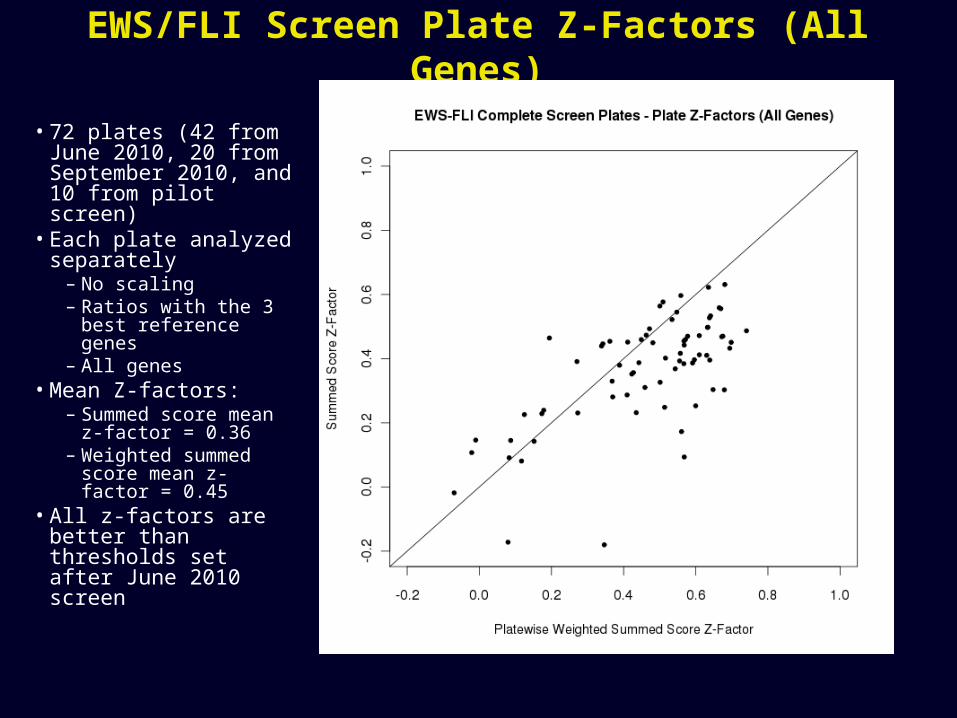
EWS/FLI Screen Plate Z-Factors (All Genes)

• 72 plates (42 from June 2010, 20 from September 2010, and 10 from pilot screen)

• Each plate analyzed separately

– No scaling– Ratios with the 3 best

reference genes– All genes

• Mean Z-factors:– Summed score mean

z-factor = 0.36– Weighted summed

score mean z-factor = 0.45

• All z-factors are better than thresholds set after June 2010 screen

EWS/FLI Screen Plate Z-Factors (Good Genes)




reference genes– Good genes

• Mean Z-factors:– Summed score mean

z-factor = 0.35– Weighted summed

score mean z-factor = 0.51

• All z-factors are better than thresholds set after June 2010 screen

Fraction of Genes Changing in Expected Direction





• Mean fraction of genes changing in expected direction = 0.74

• All plates have 65% or more of all genes changing in expected direction


0

2

4

6

8

10

12

14

16

18

20

0.5

0.54

0.58

0.62

0.66 0.7

0.74

0.78

0.82

0.86 0.9

0.94

0.98

Fraction of Genes

Nu

mb

er o

f P

late

s






• Mean fraction of genes changing in expected direction:

– Up genes = 0.84– Down genes = 0.56– All genes = 0.74

• The balance of up and down genes changing varies considerably

Histogram of Z-Score of Summed Scores (Good Genes)



– No scaling– Ratios with the 3

best reference genes

– Good genes

• Summed score z-score normalized after calculation so plate data can be compared

Histogram of Z-Score of Weighted Summed Scores (Good Genes)





– Good genes– Plate specific

weights• Weighted summed

score z-score normalized after calculation so plate data can be compared

Hit Distribution (Good Genes)



– Ratios with the 3 best reference genes

– Good genes– Plate specific weights

• 5 methods for calling hits

– Summed score probability > 0.5

– Weighted summed score probability > 0.5

– Naïve Bayes > 0.5– KNN– SVM

EWS/FLI Screen Hit Distribution

1

10

100

1000

10000

100000

Number of Methods Calling a Compound a Hit

Nu

mb

er

of

Co

mp

ou

nd

s

Compounds 40 35 39 39 94 11273

5 4 3 2 1 0

Summed Scores Hit Distribution (Good Genes)





– Good genes• Not a linear

relationship between score and probability but the best probabilities have the highest scores

Weighted Summed Scores Hit Distribution (Good Genes)




reference genes– Good genes– Plate specific weights

• Not a linear relationship between score and probability but the best probabilities have the highest scores

Hit Distribution with Scores (Good Genes)





• 5 methods for calling hits– Summed score

probability > 0.5– Summed score z-score

> 3– Weighted summed

score probability > 0.5– Weighted summed

score z-score > 3– Naïve Bayes > 0.5– KNN– SVM


1

10

100

1000

10000

100000


Nu

mb

er

of

Co

mp

ou

nd

s

Compounds 40 31 36 24 39 52 83 11215

7 6 5 4 3 2 1 0

Hit Distribution Versus Plate (Good Genes)







– Summed score z-score > 3


– Weighted summed score z-score > 3


Hit Distribution Versus Plate Pairs (Good Genes)







– Summed score z-score > 3


– Weighted summed score z-score > 3


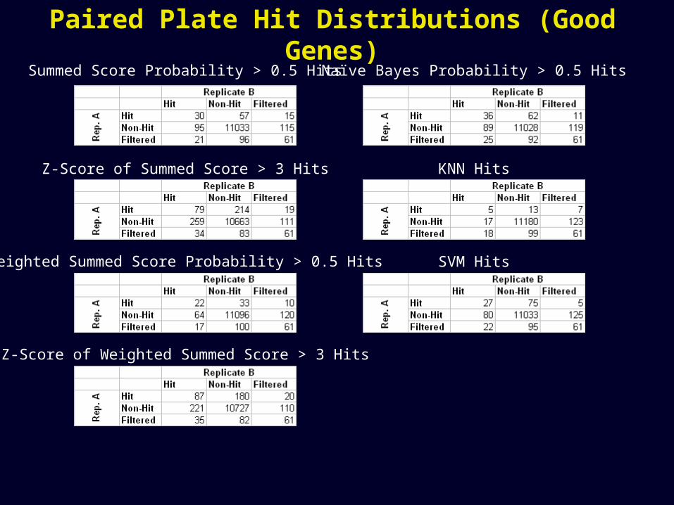
Paired Plate Hit Distributions (Good Genes)Summed Score Probability > 0.5 Hits

Z-Score of Summed Score > 3 Hits

Weighted Summed Score Probability > 0.5 Hits

Z-Score of Weighted Summed Score > 3 Hits

Naïve Bayes Probability > 0.5 Hits

KNN Hits

SVM Hits

Viability Prediction in Ewing Data• Viability prediction model developed with data from 3

development plates and pilot screen:– Cytotoxic compound plate– Compound plate from Kung lab with compounds predicted active in

Ewing sarcoma– Phenothiazine compound plate– EWS/FLI pilot screen data (5 chemical plates in duplicate from

ChemBiology)

• Viability prediction with KNN– Sample relative viability defines cells in well as either alive (>=0.2) or

dead (<0.2)– Development data split into train and test with 25% of combined data

from 3 development plates and pilot screen for training and remaining for testing

– Data Median Range Scaled together and each sample normalized (subtract median and divide by median absolute deviation)

Classifiers for Viability Prediction25% of all Data for Training – KNN – Normalized

• Ewing development plate with 25% of data from 3 development plates and pilot screen used to train a viability model

– Used day 2 viability relative to DMSO mean of day 2 viability relative to day 0 ratio

– Sample relative viability defines cells in well as either alive (>=0.2) or dead (<0.2)

– Median range scaled data– Samples normalized by

subtracting median and dividing by median absolute deviation

– KNN classifier• K=3• Cosine distance• Distance weighting• 10 features selected by signal-to-

noise

• Performance with normalization slightly better

25% Combined Training – LOOCV Results

Held-Out 75% Combined Testing

Applying Viability Prediction to EWS/FLI Screen• Ewing development plate with 25% of

data from 3 development plates and pilot screen used to train a viability model

– Used day 2 viability relative to DMSO mean of day 2 viability relative to day 0 ratio

– Sample relative viability defines cells in well as either alive (>=0.2) or dead (<0.2)

– Median range scaled data– Samples normalized by subtracting median

and dividing by median absolute deviation– KNN classifier

• K=3• Cosine distance• Distance weighting• 10 features selected by signal-to-noise

• Seems to have some success – Some known toxic compounds are

predicted dead– Probably many of the 389 of 23040

compound wells filtered would also be predicted dead

Hit Distribution with Viability (Good Genes)




– Good genes• KNN model used to

predict viability– Trained on pilot screen

and development plates


– Summed Score Probability

– Weighted Summed Score Probability

– Naïve Bayes– KNN– SVM


1

10

100

1000

10000

100000


Nu

mb

er

of

Co

mp

ou

nd

s

Pred. Alive 3 11 17 24 71 11379

Pred. Dead 37 24 22 15 23 178

5 4 3 2 1 0

Viability and Subsignature PredictionConclusions / Future Work

• Viability prediction seems to be working reasonably well– A reasonable number of wells that made it through reference gene

filtering are being classified as “dead”– Many of the hits appear to be in “dead” wells– Evaluate with secondary screen where there will be viability

measurements• More work with viability prediction

– Need to further explore methods for working across different batches of data

– How much training data is needed? Would more training data improve the models?

– What kind of training samples are needed? Can we use several standard test plates?

– Further evaluation of data scaling, use of log expression ratio, and other model types

– Try other types of classifiers, e.g., SVM and Naïve Bayes• Other work with subsignatures in GE-HTS data

Conclusions / Future Work• Quality of screen data is not ideal but workable

– Repeat plates and pilot screen plates have best quality

– Key to salvaging poor data is ability to follow-up a sufficiently large number of hits

• Analysis methods needed to accommodate data obtained from many batches and to be robust to batch variations– Analyzed plates separately and then collapsed results

• Used plate specific models for hit selection• Each plate used its own set of ‘good’ genes (plate dependant)• Fortunately 32 positive and 32 negative controls on each plate

– SVM seems to suffer the most with plate-by-plate analysis because wide separation between controls allows divergent models

– Overlap of hits between replicates suggests that the batch effect problems have been at least partially dealt with

– Can the predicted viability be used to avoid ‘hits’ that just kill the cells?

Documents

Analysis of the Full Ewing EWS/FLI Screen Ken Ross 10/22/10 The Broad Institute of MIT and Harvard