Analysis of the Circulation on the East-Chinese Shelf

and the adjacent Pacific Ocean

Dissertation

zur Erlangung des Doktorgrades

der Naturwissenschaften im Fachbereich

Geowissenschaften

der Universität Hamburg

vorgelegt von

Xueen Chen

aus Qingdao, China

Hamburg

2004

Als Dissertation angenommen vom Fachbereich Geowissenschaften der Universität Hamburg auf Grund der Gutachten von Prof. Dr. J. Sündermann und Dr. T. Pohlmann Hamburg, den 14.12.2004 Prof. Dr. H. Schleicher Dekan des Fachbereichs Geowissenschaften

2

Abstract The East-Chinese Shelf (or North East Asian Regional seas – NEAR-seas) has the broadest

shelf waters and the most complicated topography in the world. With the through-flow of one of the two largest western boundary currents – the Kuroshio - it provides an ideal case to investigate the water exchange mechanisms between shelf waters and oceanic waters, the variability of channel transports and the Joint Effect of Baroclinicity and Relief (JEBAR).

In this work, a regional numerical model has been established and a 44-year hindcast study is

accomplished with the surface flux dataset derived from ERA40 reanalysis in the NEAR-seas from 1958 to 2001. The numerical model is based on the parallelised HAMburg Shelf Ocean Model (P-HAMSOM) and features a high resolution both vertically and horizontally. The systematic verification of the regional model proves that its performance is successful, the validation data used spans from historical data of ship cruises to remote sensing data of satellite. It is expected that a nested strategy to provide more realistic inflow boundaries and an embedded ice model dealing with the ice process in northern Japan Sea will surely improve the hindcast.

The Kuroshio and its branch currents system of the NEAR-seas is investigated by means of

three approaches. An extensive analysis of the WOCE/SVP KRIG data from 1989 to 1999 reveals the surface current pattern in the NEAR-seas. A tracer model is designed to simulate the trajectories derived from the satellite tracked Lagrangian drifters. The tracer model successfully reproduces these drifter trajectories. This is a validation of the hindcast model from a different point of view by means of totally independent data. For the first time, the existence of a large eddy east of the Ryukyu archipelago is demonstrated.

The second approach is the analysis of the ocean temperature, salinity and currents based on

the model generated variable fields in the NEAR- seas. The characteristics of the climatological SST and SSS distribution are summarized. The existence of the HBCW (Huanghai Bottom Cold Water) is demonstrated and its structure in summertime is described.

The vorticity balance in the NEAR-seas is examined and the JEBAR and its role on the

East-Chinese Shelf is analyzed extensively. According to this study, JEBAR is formulated as an arithmetically generated term in the final vorticity equation. It can be a correction term to the vorticity balance only when the velocity field is in a quasi-stationary state. Many earlier works take the JEBAR for mechanism to force the currents in the real ocean. This is, however, an incorrect application of the JEBAR term. The JEBAR can only be used as a forcing term when the currents are examined in a pure diagnostic way, but even in this case it is not really forcing mechanism. The maximum and minimum of the JEBAR distribution on the East-Chinese Shelf correlates well with the shelf breaks or straits where strong currents exist. The JEBAR plays an important role in the depth-averaged vorticity balance along shelf breaks and straits where the JEBAR is two orders of magnitude larger than other vorticity terms, while it plays a minor role in shallow shelf waters.

3

4

Abstract 3

Contents 5

Preface 7 Chapter 1 Introduction 9 1.1 Morphology 9 1.2 Hydrodynamics conditions 11

1.2.1 The Kuroshio 11

1.2.2 Huanghai 11 1.2.3 The East China Sea 12 1.2.4 Taiwan Strait 14 1.2.5 The PN-line, the TK-line and the Kuroshio transport 14 1.2.6 The meander of the Kuroshio front 16 1.2.7 The Korea Strait and Japan Sea 16 1.2.8 The Kuroshio south of Japan 18 1.2.9 The Eddy field east of the Taiwan Island 20

1.3 Atmosphere conditions 20 1.4 Recent modelling work on the NEAR-Waters: A simple review 21 Chapter 2 The Model 23 2.1 A brief introduction of the model 23 2.2 Model configurations 24

2.2.1 Boundary conditions 25 Hydrographical conditions Hydrology conditions Meteorological conditions

2.2.2 Model initialization and modelling strategy 27 Chapter 3 Model validation 29 3.1 Historic observations of the NEAR-seas 29

3.1.1 Model validation using hourly sea level data 29 3.1.2 Model validation using the temperature station data 34 3.1.3 Model validation using oceanographic observations 37

3.2 Satellite remote sensing observations of the NEAR-seas 43 3.2.1 Model validation using the AVHRR Oceans Pathfinder SST 43 3.2.2 Model validation using the AVISO absolute dynamic topography 47

3.3 Summary 50 Chapter 4 The Drifter field 51 4.1 The WOCE SVP program 51 4.2 Buoys released in North East Asian Regional seas 52 4.3 Surface current features revealed by buoys 53

4.3.1 The zonal eddy zone along the southern boundary 53 4.3.2 The current pattern northeast of Taiwan Island 54 4.3.3 The frontal eddies accompanying the Kuroshio in the East China Sea 55

5

4.3.4 Anticyclonic motions southwest of Kyushu and Kuroshio branching 55 4.3.5 The water exchange across Ryukyu archipelago 65 4.3.6 Eddy field east of Ryukyu archipelago and southeast of Japan 65

4.4 The tracer model and the numerically produced tracer field 67 4.4.1 Simulation of buoys released near the eastern Taiwan Island coast 69 4.4.2 Simulation of buoys released over the East China Shelf 75 4.4.3 Simulation of buoys released in Korea Strait 78

4.5 Summary 79 Chapter 5 Discussion of the Kuroshio system in the East China Sea 83 5.1 Model generated climatology of the stream function 84

5.1.1 General pattern of the stream function field 84 5.1.2 EOF analysis of the monthly mean streamfunction 88

5.2 Simulated transport across channels in the NEAR-seas 90 5.2.1 The climatological channel transports 90 5.2.2 The monthly transport across selected channels and their variations 93

5.3 Analysis of the velocity fields in the East China Shelf 97 5.3.1 Sections across channels 102 5.3.2 Sections wrapping the East China Shelf

102 5.3.3 Sections near northeastern coast of the Taiwan Island 105 5.3.4 PN-section and sections of origination of the Tsushima Current 112

5.4 Summary 112 Chapter 6 Discussion of the temperature and salinity fields 113 6.1 Introduction: Climate signals in the Pacific 113 6.2 Model generated sea surface climatological fields 115 6.3 Long-term variations of surface fields across the PN section 120 6.4 Distribution of temperature and salinity along the PN section 123 6.5 Model simulated Huanghai Bottom Cold Water in summertime 124 6.6 Summary 129 Chapter 7 Discussion of the Joint Effect of Baroclinicity and Relief (JEBAR) 131 7.1 Introduction to JEBAR 131 7.2 Interpretation of the JEBAR-term by vorticity derivations 132 7.3 Distribution of JEBAR-term in NEAR-Seas 136

7.3.1 A simple review of JEBAR research in the NEAR-Seas 136 7.3.2 JEBAR distribution in the NEAR-Seas 136

7.4 Summary 154 Chapter 8 Summary and outlook 165 Acknowledgements 167 List of abbreviations 168 List of tables 168 List of figures 169 List of symbols 173

6

References 174

7

Preface In this work the North East Asian Regional (NEAR) Waters are defined as follows:

the continental and oceanic water areas north of 21.5oN and west of 144.5oE, this area includes the Japan Sea, Bohai, Huanghai, the East China Sea and part of the northwest Pacific Ocean. This area has the broadest continental shelf and the steepest continental slope in the world; the maximum water depth ranges from 200m on the shelf to more than 9000m east of the Ryukyu archipelago. The most striking hydrodynamic feature of this area is the through-flow of the Kuroshio. The Kuroshio and the Kuroshio Extension region lie between 25oN-50oN and 120oE-180oE, the Izu Ridge divides this system into two parts: the Kuroshio system west of 140oE and the Kuroshio Extension System east of 140oE.

This area is also a vital region, both economically and politically. Due to historical

and political reasons, in-situ oceanic investigations are rarely available compared to other marginal seas worldwide. The lack of historical data sets strong limitations for oceanographers to systemically study the Kuroshio and other oceanic phenomena here. For example, most modelling studies of the East China Sea take the Ryukyu archipelago as a closed boundary instead of an open one, since little is known east of the Ryukyu archipelago.

Fortunately, some international cooperation projects have been carried out in China

since mid-1980s, for example, the China-Japan joint Kuroshio Investigation of 1986 to 1992 and the China-Japan joint Subtropical Circulation Investigation of 1995 to 1998. With the development of global numerical ocean and atmosphere models, some general scientific databases are created, such as ERA40 (European Center for Medium-Range Weather Forecast, see Gibson et al. 1997) and the NCEP/NCAR (Kalnay 1996) reanalysis data. All these efforts make it possible to force a regional model on a relatively large research area using more realistic boundary conditions. In this work, the parallelised Hamburg Shelf Ocean Model will be applied to the NEAR-Waters to accomplish a long-term oceanic simulation, in order to improve our knowledge about the hydrodynamic conditions in this area.

In this study, some Chinese conventional names of the seas or rivers of the research

area will be used. That is, the Yangtze River will be called Changjiang, the Yellow River will be called Huanghe, the Bohai Sea (Bohai Gulf) will be called Bohai and the Yellow Sea will be called Hunaghai.

8

9

Chapter 1 Introduction 1.1 Morphology

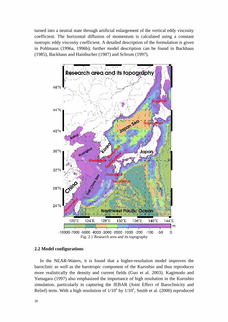
The NEAR-Waters are bounded by a very complicate morphology, see Fig. 2.1.

Over the Chinese continental shelf, three shelf seas -- Bohai, Huanghai and the East China Sea -- make up a broad shallow area with a depth of less than 200m. They are bounded by Mainland China, the Korea Peninsula, the Okinawa trough and Taiwan Island (Fig. 2.1). This area is nearly isolated from the open ocean by the Ryukyu archipelago. It is connected to the Japan Sea through the Korea Strait, to the South China Sea through the Taiwan Strait, to the Pacific Ocean through the Tokara Strait and the East Taiwan Strait.

As a shelf sea between Bohai and the East China Sea, Huanghai is a shallow sea

with relatively flat shelf, which is enclosed on three sides by Mainland China and the Korean Peninsula. Its long axis extends approximately 1000 km towards inland from the East China Sea, with depths of less than 100m. A central trough along this axis penetrates even into Bohai.

The continental shelf slope in the East China Sea has a gradient of 800m over

20-30 km. Along the edge of the East China Sea exists the shelf slope and the Okinawa Trough. From south to north, the depth of the Okinawa Trough decreases from more than 2000m to less than 1000m. The east flank of the Okinawa Trough is the Ryukyu archipelago, which separates the Chinese shelf from the Pacific Ocean. East of Taiwan Island, the bottom topography rises abruptly from a depth of more than 3000m south of 24oN to a depth of less than 200m north of 24oN. The depth of the Dayu Strait is between 100m to 200m, while the depth of the Tokara Strait varies from 500m to 1000m.

South of Japan and east of the Ryukyu archipelago stretches the Pacific Ocean with

a maximum depth of more than 9000m. The Izu Ridge cuts this ocean area into two basins: the Philippine Basin and the Northwest Pacific basin.

The Japan Sea lie between the Asian continent and Japan as a marginal sea with

depths of 3700m over most of its area. It is connected to the East China Sea in the south through the Korea Strait, to the Sea of Okhotsk in the north through the Mamiya strait, and to the Pacific Ocean in the northeast through two relatively narrow, shallow straits – the Tsugaru Strait and the Soya Strait.

10

1.2 Hydrodynamic conditions 1.2.1 The Kuroshio

Originating as the northward flow at the western boundary in the bifurcation of the

North Equatorial Current, the Kuroshio begins east of the Luzon Island and is the western boundary current of the north Pacific subtropical gyre. The Kuroshio flows northward into the East China Sea through the East Taiwan Strait, then it sets northeastward along the East China Sea shelf slope west of the Ryukyu archipelago. The west boundary here is actually the broad shelf, the Kuroshio extends to the bottom and there exists a narrow southwestward recirculation on each side. Near the latitude of 30oN, the Kuroshio veers eastward near 30oN and 128-129oE and passes through the Tokara strait, then it flows along the Japan coast until it separates from the coast at 35.0oN, 140.0oE, and enters the Northwest Pacific basin as a free jet called the Kuroshio Extension. Free from the constraint of coastal boundaries, the Kuroshio Extension has been observed to be an eastward flowing inertial jet accompanied by large-amplitude meanders and energetic pinched-off eddies (Yasuda et al. 1992).

The large-scale ocean circulation is driven both by windstress forcing and by

fluxes of heat and freshwater at the ocean surface. The ocean moderates climate through its large thermal inertia, its large heat capacity and its poleward heat transport by the ocean currents. The total meridional heat transport of the global ocean is about the same as that of the atmosphere, with the North Atlantic and the North Pacific heat transport being polarward and of the same order of magnitude. Due to the absence of a vigorous gravitational overturning at high latitudes in the North Pacific Ocean, the Kuroshio is a much more important poleward carrier of heat and salt in the North Pacific Ocean than the Gulf Stream is in the North Atlantic Ocean (Roemmich and McCallister 1989; Bryden et al. 1991). According to Bryden et al. (1991), the heat transport by the Kuroshio is about half the ocean heat transport across 24oN in the northern Pacific. Therefore, ocean circulation changes in the NEAR-Waters can affect the global climate substantially.

On the one hand, the Kuroshio variability as a result of its interactions with the

East China Sea is of crucial significance and must be understood if climatic changes, regional or global, are to be resolved. On the other hand, heat and salt from the Kuroshio dominate water mass formation in the marginal seas and, through cooling at high latitudes, may even provide a source for the formation of the North Pacific Intermediate Water (Talley 1993). It is obviously of equally crucial significance, that the East China Sea circulation, as a result of the Kuroshio through-flow, is charted and elucidated. Thus the understanding of the local Kuroshio dynamics in the NEAR-Waters will lead to an improved predictability of the regional ocean-atmosphere interaction.

11

1.2.2 Huanghai The two distinct hydrographic structure features of Huanghai are the Yellow Sea

Warm Current extending northward as far as Bohai, and the Yellow Sea Bottom Cold Water, a water mass regarded as the remnant of winter cooling and mixing. The Yellow Sea Warm Current Water is characterized by a temperature less than 13 to 15oC and a salinity of 34.2 to 34.5 psu. Hydrographic conditions in Huanghai are strongly associated with winter cooling and summer heating, fresh water input from rivers into the coastal area, precipitation and advection of warm saline water from the south by the Kuroshio and Taiwan Warm Current.

Strong northerly winds prevail over Huanghai during winter months, while the

summer is characterized by weak southerly winds. During winter, wind-generated turbulence enhances deep cooling by thermal convection. When water is vertically homogeneous, the southern Huanghai water masses are classified into two types: the low temperature and salinity Yellow Sea Bottom Cold Water in the lower layer, the high temperature and salinity Yellow Sea Warm Current Water in the upper layer. The Yellow Sea Bottom Cold Water is characterized by a temperature less than 10oC and a salinity of 32.5 to 33.0 psu. As we know, the Yellow Sea Bottom Cold Water is formed during winter by severe cooling in Huanghai. It stagnates under the seasonal thermocline from spring to late summer in the deeper area of Huanghai, moving southward, its southern limit sometimes reaching as far as 30oN. The southward Yellow Sea Bottom Cold Water reaches its maximum southern position in April. During summer, the weaker and less persistent winds combine with surface heating to produce a very strong thermal stratification, isolating the bottom Yellow Sea Cold Water. When a thermocline is well established near 30m depth, another two water masses join here: Changjinag Diluted Water and coastal waters.

The circulation pattern in Huanghai is predominantly seasonal. The winter and

summer circulation are partitioned dynamically between tidal rectification, baroclinic pressure gradients, wind response and river discharge from Changjiang. Wind dominates the pattern of wintertime. In summer, baroclinic pressure gradients dominate the eastern part; tidal rectification, wind and river discharges dominate the western part.

In winter, the strong northwesterly winds force nearshore and surface transport

southward, demanding a northward return flow at depth. This flow is thought to originate from the warm salty Taiwan Warm Current and explains the observed Yellow Sea Warm Current. Nearshore currents are southward of both the Chinese and Korean coasts. In summer, the dense Yellow Sea Cold Water dominates in the central Yellow Sea, resulting in a basin scale low-pressure system and a cyclonic circulation. Wind forcing is in the opposite direction relative to winter and significantly reduced, resulting in an interruption of the northward flow associated with the Taiwan Warm Current. Under this scenario, coastal currents are directed northward along the Korean

12

coast and southward along Mainland China. Earlier there existed two different concepts concerning the origin of the northward

flow in the Huanghai trough -- the so-called Yellow Sea Warm Current. The first concept is its branching from the northward Kuroshio branch southeast of Cheju Island (Nitani 1972; Guan and Mao 1982). The second is its branching from the Taiwan Warm Current southwest of Cheju Island (Beardsley et al. 1985). In recent studies, however, the Yellow Sea Warm Current is thought to be just a return flow in compensation of wind-driven coastal currents setting southward (Hsueh et al. 1997). These authors argued that during fall transition and winter monsoon periods, strong northerly wind bursts drive an increasing of the north to south pressure gradient extending from the Yellow Sea Trough over to the Korean coast and force this northward flow in the trough. This flow does not seem to extend into Huanghai as previously believed. For example, at least in the summer of 1983 and 1984, it rather turns clockwise eastward to the Cheju Strait around the northwest coast of the Cheju Island.

The Cheju Warm Current was defined as a mean current that rounds the Cheju

Island clockwise with speeds of 5 to 40 cm/s, transporting warm and saline water to west coast of the Cheju Island and into Cheju Strait throughout the year. It is partly formed by Tsushima Current waters (Chang et al. 2000). In summer and autumn the Cheju Current appears only in the lower layer, retreating in the west coast of the Cheju Island in summer and to the east coast of the Cheju Island sometimes in autumn.

The Changjiang Diluted Water affecting Huanghai is another factor. Changjiang is

the dominant river contributing approximately 90% of the composite inflow from the five rivers in the region with an annual mean discharge of 28,900 m3/s (Riedlinger and Preller 1995). The monthly flow rates of Changjiang vary from 9,300 to 5,400 m3/s, corresponding to July and January, respectively. The average discharge of the Changjiang is about 10,000 m3/s in winter and 50,000 m3/s in summer. During winter the Changjiang discharge exits southwestward along the Chinese coast, while in summer a more variable and intense discharge spreads offshore more than 550 km towards northwest to Cheju Island without losing its hydrographic properties. The Huanghe, which discharges into Bohai with an annual flow of approximately 1/20 of that for the Changjiang, also has an important influence on Huanghai via a southward current along the Chinese coast.

The tides in Huanghai are mainly mixed diurnal and semidiurnal with M2 and K1

amplitudes of order 1.0 and 0.25m, respectively. In some regions tidal currents are sufficient to create permanent mixing fronts. Rectification of large tidal current nearshore is likely to contribute to subtidal circulation patterns year-round.

1.2.3 The East China Sea

13

The East China Sea contains a broad continental shelf and a major western boundary current, the Kuroshio, along its outer shelf edge. Over the East China Sea, the surface wind forcing changes on seasonal and synoptic scales (Beardsley et al. 1985). The SST of the East China Sea ranges from 27oC to 29oC in summer, the strongest front usually occurs in May. From cluster analysis (Kim et al. 1991), the annual wintertime cooling and summertime heating results in maximum surface temperatures of 20oC in the northern reaches. Two largest rivers in the world, the Changjiang and the Huanghe influence the East China Sea. The Changjiang discharges directly into the East China Sea, the Huanghe influences the salinity field of the East China Sea considerably. Because of this annual SST variability and the large river discharge, the East China Sea Water is noticeably cool and fresh in the mean (Levitus 1982). In contrast, the upper thermocline waters of the Kuroshio are warm and saline, being dominated by the subtropical mode water of the central North Pacific (Nitani 1972; McCartney 1982; Tsuchiya 1982), which are formed in the mid-latitude regions where evaporation exceeds precipitation, resulting in a warm and saline water mass.

The Kuroshio enters the East China Sea through the East Taiwan Strait between

Taiwan and Yonakunijima Island, the western tip of the Ryukyu archipelago. It then flows northeastward along the continental shelf break to 30oN. There, part of the flow on the left-hand side of the Kuroshio separates as the Tsushima Current (Sverdrup et al. 1942). The main flow continues eastward out of the East China Sea through the Tokara Strait.

Long-term geomagnetic electrokinetograph (GEK) measurements reveal a seasonal

migration of the Kuroshio main axis northeast of Taiwan Island (Sun 1987). The Kuroshio migrates both seasonally and intra-seasonally, with the former mode being more pronounced, shoreward in fall and winter, seaward in spring and summer. Hsueh et al. (1992) indicated that the Kuroshio main axis moved closer towards the shelf from late fall to next spring and shifted seaward in summer.

The flow pattern north of Taiwan Island is significantly impacted by this seasonal

migration. In summer the Kuroshio generally moves away from the shelf, colliding with the shelf breaks of the East China Sea and splitting into a northwestward branch current and an eastward main stream. Southwest of the branch current, a counterclockwise circulation was produced along the northern shelf edge of the northern shelf of Taiwan Island, through which the subsurface Kuroshio water intruded forming a cold dome. In winter the Kuroshio moves close to and sometimes onto the northern shelf of Taiwan Island. The intrusion of the Kuroshio dominates the flow pattern in the region, causing the disappearance or obscuration of the counterclockwise circulation and cold dome in the summertime.

Observations of the hydrography and water movements in the East China Sea in

areas where the bottom topography interacts with the Kuroshio indicate a vigorous

14

water exchange between the Kuroshio and a continental shelf water mass that is relatively cool and fresh. The Kuroshio intrudes into the East China Sea preferably at two locations: one is northeast of Taiwan Island, where the subsurface Kuroshio water upwells onto the shelf while the main current deflects seaward; the other is near 31.0oN, 128.0oE.

The modification of the upper thermocline occurs primarily along the continental

shelf break south of 28oN, where the subsurface water of the Kuroshio is uplifted along a stretch of the continental shelf break, generating a surface-layer circulation featuring a flow of cool and less saline shelf water towards the Kuroshio. This movement in the vertical creates strong mixing that is of particular importance in chemical and biological oceanographic terms because of the involvement of nutrient-rich subsurface waters. Thus there is a convergence of continental shelf water towards the Kuroshio in the surface layer south of 28oN, to the southwest of Kyushu Island.

Near 31oN, the shoaling topography of the Kyushu coast, towards which the

Kuroshio flows almost at a right angle of incidence, is soon to exert its influence. This influence is already evident more than 200 km upstream at about 30oN, in the beginning of an anticyclonic turn in the Kuroshio and in the separation of part of its flow on the left-hand side. Here the Kuroshio is directed towards the coast of Kyushu and is forced to turn eastward. This divergence leads to the formation of the Tsushima Current and supplies the water mass for the Yellow Sea Warm Current. These currents transport tropical heat and salt hundreds of kilometers to the north and are important for the water mass formation in these northern reaches of the marginal seas and, via the Japan Sea and Okhotsk Sea, for the maintenance of the stratification of the North Pacific Ocean. 1.2.4 Taiwan Strait

The mean Taiwan Strait water transport estimates range from less than 0.5 to 1.0 Sv1 (Wyrtki 1961) to 2.0 Sv (Zhao and Fang 1991). Chang et al. (2001) suggested that the water transport through Taiwan Strait is 2.0 Sv in May and 2.2 Sv in August. While Teague et al. (2003) suggested a much smaller transport for October-December, 1999, in this time period the average volume transport is 0.14 Sv through Taiwan Strait.

The current meter observations in the central and southern Taiwan Strait (Chuang

1986) reveal the flow there to be generally northward. A southward current was found only when the northeasterly monsoon intensified and maintained its strength for several days. 1.2.5 The PN-line, the TK-line and the Kuroshio transport 1 1 Sv =1 x 106m3/s

15

The Kuroshio traverses a series of ridges upon entering and exiting the East China

Sea, the east Taiwan Strait is nearly perpendicular to the Kuroshio path and has a sill depth of about 750m (Smith and Sandwell 1997).

The PN-line denotes a fixed line across the Kuroshio in the central East China Sea

from northwest (30.0oN, 124.5oE) to southeast (27.5oN, 128.25oE), see Fig. 3.6. The Japan Meteorological Agency has made quarterly hydrographic observations along this fixed line since 1972.

Along the section of the PN-line the warm Kuroshio waters move onto the shelf at

a typical speed of 0.1 to 0.2 m/s. Across the PN-section the Kuroshio has a single stable current core located on the continental slope.

The Kuroshio at the TK line (i.e. the Tokara Strait line, see Fig. 3.6) has a double

core structure over the two gaps of the Tokara Strait. During the large meander period the northern core is much stronger than the southern core on average, while the difference is small during the non-large-meander period (Oka 2003).

On the PN-line section a significant maximum of potential vorticity is located just

onshore of the current axis in the middle part of the main pycnocline. Along the TK-line, potential vorticity is small and nearly uniformly distributed predominantly during the non-large-meander period and is closely related to the generation of the small meander of the Kuroshio southeast of Kyushu.

The Kuroshio has a relatively low transport near its origin, being augmented along

its path by additional flow from the east. The Kuroshio volume transport shows an interdecadal variation, small before 1975 and large afterward. Based on 34 cruises, Gilson et al. (2002) calculated the mean geostrophic Kuroshio transport across 21.5oN. They concluded that from surface to a depth of 800m, the Kuroshio transport is 22.0 Sv ± 1.5 Sv. The Kuroshio appears to be confined mainly to the upper 700m and is usually contained between 120.85oE and 121.75oE there.

Yuan et al. (1998) proposed that the net northward volume transport southeast of

Taiwan Island is 44.4 Sv. A branch current of the Kuroshio flows northeastward to the east of Ryukyu archipelago. East of Ryukyu archipelago exists an anticyclonic recirculation. The volume transport of the east Ryukyu Current is 15.6 Sv.

Ichikawa et al. (2000) suggested that the total transport across the PN line is 25.9

Sv in spring, 23.5 Sv in fall and 28.5 Sv in summer. Based on the in situ observation data, Yuan et al. (1998) concluded that the northeastward transport across the PN line in the East China Sea is 27.2 Sv.

Based on the difference between the sea surface dynamic topography across the

16

Kuroshio derived from TOPEX/POSEIDON altimeter data for 1992-1999, Imawaki (2001) concluded that the Kuroshio transport south of Japan, excluding contributions by local recirculation, is 42 Sv on average. Considering the contribution by the recirculation, the value is around a mean of 57 Sv. Qiu and Joyce (1992) estimated a zonal mean geostrophic transport of the Kuroshio across 137oE as 52 Sv.

1.2.6 The meander of the Kuroshio front

The features of warm, tongue-like extrusions of the Kuroshio which are oriented

southwestward around cold upwelled cores have been frequently observed in infrared image from satellites. Such features are related to the meander of the Kuroshio front along the edge of East China Sea. Sugimoto et al. (1988) found that the wave period of the meander of the Kuroshio front in East China Sea was 11 to 14 days. The wavelength of this meander is 300 to 350 km and phase speed 30 cm/s. Qiu et al. (1990) reported that the typical period of the meander of the Kuroshio front is 14 to 20 days, its wavelength 100 to 150 km and phase speed 20 to 26 cm/s.

Based on the CTD, ADCP and satellite-tracked drifters observations, Yanagi et al.

(1998) found that the length and width of the cold core of the Kuroshio frontal eddy were about 60 and 40 km, respectively. Its phase speed was about 30 cm/s. The center of the frontal eddy shifted offshore in the deeper layer. Across the shelf edge, nutrients were advected onshore by passing the frontal eddy, whereas they are advected offshore without the actions of frontal eddies.

1.2.7 The Korea Strait and Japan Sea

Cheju Island is located at the western tip of the Korea Strait. The strait between

Cheju Island and Korea Peninsula is named the Cheju Strait. The island in the middle of the Korea Strait is Tsushima Island. The Tsushima Current is partly formed on the continental shelf between the southern East China Sea and Cheju Island, it is not just physically separated from the Kuroshio but has distinct origins.

There are two different schools of thought about the origin of the Tsushima Warm

Current: 1) it comes from Taiwan Strait or 2) from the Kuroshio southwest of Kyushu Island. When veering eastward near 30oN, a small portion of the Kuroshio transport remains west of Japan, entering the Japan Sea as the Tsushima Current.

Based on a temperature data set from 1961 to 1990, monthly maps of horizontal

heat transport show the existence of the Taiwan-Tsushima Warm Current system from April to August (Isobe 1999b). Isobe confirmed, except for autumn, the existence of the so-called Taiwan-Tsushima Current (Fang et al. 1991). Only in autumn about 66% of the Tsushima Current transport comes directly from the Kuroshio crossing the shelf edge of the East China Sea.

17

There are also two general concepts about the Tsushima Current pattern after it enters the Japan Sea: One is that the current consists of two or three branches, the other is that it is a meandering current. To reconcile these two opinions, Kawabe (1982) suggested that the Tsushima Current splits into three branches as it enters the Japan Sea, one of the three branches developing into meanders in the interior of Japan Sea. A contradiction to the historical concept of this branching is that, in the spring of 1981 the Tsushima Current did not split as it exited from the Korea Strait and flowed into the Japan Sea. Cho et al. (2000) found that the branching of the Tsushima Current was absent in February from 1989 to 1992. During the springs of 1982 and 1983, however, the branching was evident from satellite images, one branch flowed northward along the Korean coast, it changed its direction abruptly to the east at about 37oN, the other flowed eastward along Honshu Island.

The absence of the East Korean Warm Current bears an exceptional importance not

only on the branching mechanism but also on the circulation in the Japan Sea. Using a two-active-layer hydraulic model, Cho et al. (2000) investigated the dynamics of the branching mechanism of the Tsushima Current in the Korea Strait. They found that the westward intrusion of the bottom layer cold water to the Korea Strait decides the branching of the Tsushima Current. Johnson et al. (2002) argued that when the geostrophic transport of the Tsushima Current is low the cold bottom water intrudes, and vice versa.

The most striking feature of the Japan Sea is the contrast of water masses across

the polar front, which separates it into two regimes (Jacobs and Hogan 1998). The northwestern regime is affected by sea ice processes, river run-off and deep convection, while the southeastern regime is warm and rich of chlorophyll fed by the Kuroshio water.

The Japan Sea is also one of the most eddy-rich areas in the world. The typical

horizontal scale of eddies in the Japan Sea is about 100 to 150 km (Isoda et al. 1991; Park and Chung 1999). Based on the TOPEX/POSEIDON and ERS-2 altimetric data, Morimoto et al. (2000) found that the Yamato Basin and Tsushima Strait are the most energetic regions with high RMS variability of about 10 cm. The lifetime of warm and cold eddies in the Yamato basin is about 9 months.

The major warm current in the Japan Sea is the Tsushima Current. The Tsushima

Current exhibits complex branching as it meanders over the Japan Sea Proper Water south of the polar front towards the Tsugaru Strait and the Soya Strait. The Tsugaru Warm Current is the remaining flow of the Tsushima Warm Current subtracted by the Northward Current which is the northward branch of the Tsushima Warm Current west of Tsugaru Strait. It was found that throughout the year the Tsugaru Warm Current has near steady transport, fluctuations in the Tsushima Current are transmitted to the Northward Current. Its volume transport exhibits large interannual variations sometimes exceed its seasonal variations. Baroclinic structures reached deeper in

18

April and the current axis tended to shift in a near-shore direction in October. Beyond the Tsugaru Strait, part of the Northward Current joins the cold water from

the Sea of Okhotsk, then recirculates southwestward along the Russian coast and Korean coast, forming a large cyclonic circulation pattern around the deepest part of the basin.

Based on in situ CTD observations, Onishi (1997) calculated the transports through

the Tsugaru Strait with a reference depth of 800m. He found that the average volume transport from 1986 to 1993 of the Tsushima, Northward and Tsugaru Currents were 2.73 Sv, 1.39 Sv and 1.47 Sv, respectively. The Tsugaru Current transport corresponds to about 55% of that of the Tsushima Current. The minima of the Tsushima, Northward and Tsugaru Currents were 1.83 Sv (April, 1992), 0.24 Sv (April, 1992) and 0.93 Sv (April, 1989), respectively. While the maxima of the Tsushima, Northward and Tsugaru Currents were 4.13 Sv (October, 1993), 2.44 Sv (October, 1993) and 2.67 Sv (April, 1993), respectively.

1.2.8 The Kuroshio south of Japan

The Kuroshio south of Japan takes three typical alternative paths: the near shore and offshore non-large-meander (NLM) paths and the typical LM (large meander) path (Kawabe 1995). As a result of an interaction of the current with the sharp coastlines and a shallow ridge, a semi-permanent recirculating region forms between the Kii Peninsula and the Izu Ridge. During its NLM state, the Kuroshio flows along the southern coast of the Japan then separates from the coast near the Kii Peninsula and reattaches north of the Izu Ridge. The short-term Kuroshio meander formation during the non-large-meander state should be distinguished from the LM formation (Waseda et al. 2003). The Kuroshio separates from the Japan coast southeast of Honshu, usually undergoing a large northward meander and producing a warm core ring. East of Japan, the Kuroshio keeps a mean latitudinal position at about 35oN up to 180oE. (Qiu and Joyce 1992).

The amplitude of the offshore displacement of the Kuroshio west of Kii Peninsula

changes as a result of mesoscale perturbations. Satellite SSH and SST observations (TOPEX/Poseidon: T/P and NOAA AVHRR) suggest that the short-term Kuroshio meander formation is triggered by anticyclonic eddies originating in the Kuroshio Extension (Waseda et al. 2003). Ebuchi et al. (2000) found that the cyclonic and anticyclonic eddies originating from the east have a diameter of 500 km and a temporal scale of 80 days. They propagate westward with a phase speed of 6.8 cm/s.

Based on the daily and monthly mean sea levels from 1964 to 1992 of nine tide

gauges along the Kuroshio, Kawabe (1995) found that after a long time of non-large-meander paths during 1963-75, the Kuroshio took a large-meander path during most time of 1975-91: 1975-80, 1981-84, 1986-88 and 1989-91, whereas in the

19

1990s, the Kuroshio preferred a non-large-meandering state (Qiu and Miao 2000). According to Qiu and Miao (2000), the Kuroshio path variations south of Japan are

not necessarily controlled by the external inflow changes. They proposed that the observed alternations of the Kuroshio’s two states are due to a self-sustained internal oscillation involving the evolution of the southern recirculation gyre and the stability of the Kuroshio current system, rather than being controlled by the temporal changes of the upstream transport. Variations between a straight path and a meander path are found on interannual timescales, when the wind forcing is strong enough. As the intensification of the recirculation gyre progresses, it eventually leads to the meander due to baroclinic instability. Similar to the conclusions of Qiu and Miao, Hurlburt et al. (1996) found that the meander path depends on the occurrence of baroclinic instability west of the Izu Ridge. Increases in wind forcing on interannual timescales give rise to a predominant meander path, while decreases yield a predominant straight path.

Using a two-layer model, Endoh (2000) studied the trigger mechanism of the

Kuroshio meander, he found that the generation of the trigger meander southeast of Kyushu is associated with the increase in the supply of cyclonic vorticity induced by the enhanced velocity in the upper layer. He concluded that the baroclinic instability is the dominant mechanism underlying the rapid amplification of the eastward propagating trigger meander.

Kawabe (1995) proposed that the formation and decay of the large mechanism are

associated with the Kuroshio velocity and main axis in the Tokara Strait south of Kyushu. A small meander, precursor of the large meander, is formed southeast of Kyushu in connection with a temporary Kuroshio velocity increase and a northward axis shift in the Tokara Strait. An eastward propagation of the small meander, leading to the large meander formation, is associated with the axis remaining in the northern strait, but not with large velocity except in 1975. Decay of large meanders begins with large velocity and an axis return to the southern strait. Large meanders begin (terminate) about four months after the Kuroshio shifts northward (returns southward). Kawabe (1995) calculated the Kuroshio transport using the daily and monthly mean sea levels, and suggested that the large meander appears when the transport increases from about 24 Sv, while a non-large-meander is formed whenever its transport is less than 23.5 Sv.

As a return flow compensating for the wind-driven subtropical interior circulation,

the Kuroshio originates at a southern latitude (~15oN) where the ambient potential vorticity (PV) is relatively low. For the Kuroshio to smoothly rejoin the Sverdrup interior flow at the latitude of the Kuroshio Extension, the low PV acquired by the Kuroshio in the south has to be removed by either dissipative or nonlinear forces along its northward boundary path. For a narrow boundary current such as the Kuroshio and its extension, scaling analysis indicated that the dissipative force alone is not sufficient to remove the PV anomalies (Pedlosky 1987; Cessi et al. 1990). This

20

results in the accumulation of the low PV water in the northwestern corner of the subtropical gyre, which generates a mean anticyclonic recirculation gyre and provides an energy source for flow instabilities (Qiu and Miao 2000). The Kuroshio Extension and its recirculation gyre form an interconnected dynamical system. The structure change of the Kuroshio Extension system is mainly due to two factors: The basin-wide external wind forcing and the nonlinear dynamics associated with the inertial recirculation gyre.

Using available temperature measurements of 1950-70, Yamagata et al. (1985)

showed that, on interannual time scales, the baroclinic transport of the Kuroshio Extension had a lagged positive correlation with that of the upstream North Equatorial Current. Following individual ENSO events when the NEC transport increases, the Kuroshio Extension tends to intensify 1.5 years later.

By analyzing hydrographic and XBT data from 1976 to 1980, Mizuno and White

(1983) showed that the Kuroshio Extension was displaced southward, from 36-37oN during 1977-1978, to 34oN in 1979-80. Based on altimetry data from the Geosat and ERS-1 missions, Jacobs et al. (1994) noted that the Kuroshio Extension path shifted northward in 1992-93, as compared to 1987-89. They suggested that this shift resulted from the passage of a westward-moving warm Rossby wave originating from the 1982/83 equatorial ENSO event. Toba et al. (1999) found that from winter 1996 to summer 1997 the Kuroshio Extension took a very southerly path along about 34oN, they proposed that this was related to the connections of the large scale atmosphere-ocean system, such as the shift from La Niña to El Niño in 1997.

1.2.9 The Eddy field east of the Taiwan Island

Taiwan Island is impinged on by both cyclonic and anticyclonic westward propagating mesoscale eddies originating in the interior ocean at an interval of 100 days. An approaching anticyclonic (cyclonic) eddy will result in a large (small) Kuroshio transport. The decrease of the Kuroshio transport means a leakage of the Kuroshio water to the east of Ryukyu archipelago. This 100-day rate of eddy-impingement invalidates any observations of 4 months or less, whether with direct or indirect measurements, because any conclusion depends on the presence or absence of eddies (Yang 1999). At 23oN the northern part of a westward propagating mesoscale eddy is captured into the Kuroshio south of Okinawa, moves downstream, passes the Tokara Strait and reaches the ASUKA (east of the Tokara Strait) line where it merges with other eddies propagating westward at 30oN.

The Kuroshio variation at the ASUKA line is, however, directly affected by eddies

propagating from the east, not by the upstream in the south. The Kuroshio axis in the Tokara Strait is governed by short-term variations locally confined to the Kuroshio in the East China Sea, but not by the variations induced by mesoscale eddies from upstream or downstream (Ichikawa 2001).

21

1.3 Atmosphere conditions

Research of the climatology of the NEAR-Waters is rather difficult because of the complicated ocean and atmosphere dynamics associated with the Kuroshio and the Asian Monsoon. Apparently, for the local ocean-atmosphere dynamics like the Kuroshio variability in the East China Sea, monsoon is an important factor. Current meter observations made around the Minghua Canyon showed that shelf intrusions of the Kuroshio occur about one month later than the intensification of the winter monsoon (Tang et al. 2000).

ENSO, known as an interannual variation of the SST in the central and eastern

equatorial Pacific, also has an effect on the atmosphere circulation at midlatitudes and the Asian Monsoon (Kawamura et al. 1998). One argument is that the NEAR-Waters have a significant coherency with the El Niño 3.42 SST at 2 to 3 years periods with a phase lag 5 to 9 months in the SST anomaly (Park et al. 2000).

Akitomo et al. (1996) proposed that the Kuroshio transport in the East China Sea is

related to wind stress forcing in the latitude band further south, since an additional transport by wind forcing at the latitude of the East China Sea is constrained by topography to stay east of Ryukyu archipelago.

From the above description, it is concluded that the East China Shelf circulation

and the Kuroshio variability are tightly connected to the Asian Monsoon as well as the global climate changes.

1.4 Recent modelling work on the NEAR-Waters: A simple review

Among the numerical models of the tidal sea level changes and the tidal currents in

the East China Sea, some are based on the boundary value method, which calculates the tide in the domain using harmonic constants along the coast and ignoring nonlinear effects. Other models are based on time stepping methods, which reproduce the tides in the domain from the harmonic constants along the open boundary, as an instationary process, for example, the HAMburg Shelf Ocean Model (HAMSOM). The calculation of the bottom friction stress may be the most important problem in the tide model. A widely used value for the bed drag coefficient of the quadratic friction rule is 0.0026, where the quadratic friction rule calculates the bottom friction stress from the velocity at a certain height using the given bed drag coefficient.

Guo (1998) investigated the vertical distribution of tidal currents in Huanghai. He

found that as the tidal current becomes strong, its vertical shear becomes large and its vertical profile becomes sensitive to the vertical eddy viscosity. For the East China Sea, Lee et al. (2002) found a bottom friction coefficient of 0.0035 to be the optimum value. With a 3-dimensional and barotropical model forced by the M2 tide prescribed 2 The area averaged SST means between 5oN-5oS and 120oW-170oW

22

at the open boundaries, they concluded that the tide-enhanced bottom friction effectively blocks the penetration of the northwestward Yellow Sea Warm Current. The tidal residual currents omnipresent off the shallow Chinese coast between 32oN and 34.5oN contribute to suppress the Yellow Sea Warm Current formation.

The diagnostic Bryan-Cox model of general ocean circulation was adapted to the

East China Sea to study the climatological through-flow of the Kuroshio by Hsueh et al. (1997). They designed the resolution of the model domain with 1/6o horizontal grid size and 30 vertical levels. The model is driven by steady inflow and outflow that calculated from the annual mean windstress field over north Pacific, no locally imposed windstress is considered. Temperature and salinity at the sea surface are relaxed to the climatological values during the whole simulation. In the final quasi-steady field they got, the model exhibits some patterns evident in observations, such as a sharpened Kuroshio front over the upper continental slope and the separation of the Kuroshio at about 30oN.

Seung (1999) studied the dynamics of gravity-forced intrusion of the oceanic upper

layer water onto the shelf across a depth discontinuity using a simple geostrophic adjustment model. He found that the external parameters affecting the intrusion of the oceanic upper water are the difference in surface elevation between the shelf and the oceanic regions, the relative density difference between two water masses and the bottom depth of the shelf. The sea level difference moves the frontal system shelfward through a barotropic effect whereas the density difference increases the frontal width through a baroclinic effect.

Christopher et al. (2001) adapted a 3-D climatological model and simulated the

velocity field of Bohai and Huanghai for a series of six bimonthly realizations. The forcing field includes seasonal hydrography, seasonal mean wind and seasonal river input of Changjiang as well as tides. They found that winter and summer results exhibit two distinct circulation modes and are partitioned dynamically among tidal rectification, baroclinic pressure gradients, windstress and river input.

A recent prognostic simulation concerning the East China Sea was done by Guo et

al. (2003). Using the triply nested ocean general circulation model POM, they examined how the horizontal model resolution influences the Kuroshio and the sea level variability in the East China Sea. They found that as the model resolution increases from 1/2° to 1/18° the path, current intensity, vertical structure of the simulated Kuroshio and the variability of sea level become closer to observations. It is also concluded that these improvements result in a better reproduction of the interaction between baroclinicity and bottom topography.

Although many modelling studies are carried out for the research area, most of

them are forced by climatological field data or for a strongly simplified topography or as a diagnostic study. In this investigation, a fully 3-D prognostic long-term

23

simulation with six-hourly surface flux atmosphere forcing will be accomplished.

24

Chapter 2 The Model 2.1 A brief introduction of the model

An appropriate numerical model used to study the Kuroshio dynamics should be capable of resolving dynamic processes dictated both by the sharply changing topography of the continental margin and by the focusing flow in an inertial current. The eddy-resolving hydro-thermodynamical model employed in the present investigation is HAMSOM (Backhaus 1985; Pohlmann 1991; Pohlmann 1996a).

HAMSOM has extensively been applied to shelf seas worldwide, and has

performed well in different shelf seas and their adjacent oceanic areas proved its good performance (Backhaus 1985; Backhaus and Hainbucher 1987; Stronach et al. 1993; Huang 1999; Pohlmann 1996a; Schrum 1997). Specific aspects of the model implementation are described below.

The HAMSOM used here is a modified version of a three-dimensional baroclinic

level-type shelf sea model, which was initially developed by Backhaus (1985). The governing primitive equations include the shallow water equations in combination with the hydrostatic assumption, the equation of continuity and the transport equations for temperature and salinity as well as the equation of state for seawater. The numerical scheme is based on an Arakawa C-grid. The model feature concerning the long-term simulations is the sophisticated semi-implicit numerical scheme, which can free the model from the most restricting stability limitations present for explicit numerical schemes due to the propagation of external gravity waves. The implicit algorithms are applied to external gravity waves, vertical shear stress terms in the equations of motion and vertical diffusion of ocean temperature and salinity. In the time domain a stable second order approximation is introduced for the Coriolis term and the baroclinic pressure gradient in the equation of motion. Incompressibility and hydrostatic equilibrium are assumed for the pressure field, incorporating the Boussinesq approximation.

In the past 20 years, HAMSOM was generalized to include the prognostic

calculation of tracer fields such as ocean salinity and ocean temperature. To calculate vertical eddy viscosity, the vertical sub-grid scale turbulence is parameterized by means of a turbulent closure approach originally proposed by Kochergin (1987) and later modified by Pohlmann (1996a). The scheme is closely related to a Mellor-Yamada (1974) level-2 turbulent closure model where vertical eddy viscosity coefficients depend on stratification and vertical current shear. With this treatment the vertical eddy viscosity is enhanced by vertical velocity shear and reduced by vertical stability. By incorporation of turbulent surface and bottom layer processes the model becomes capable of presenting a more realistic thermal stratification. Convective overturning is parameterized through vertical mixing: an unstable stratification is

25

turned into a neutral state through artificial enlargement of the vertical eddy viscosity coefficient. The horizontal diffusion of momentum is calculated using a constant isotropic eddy viscosity coefficient. A detailed description of the formulation is given in Pohlmann (1996a, 1996b); further model description can be found in Backhaus (1985), Backhaus and Hainbucher (1987) and Schrum (1997).

Fig. 2.1 Research area and its topography 2.2 Model configurations

In the NEAR-Waters, it is found that a higher-resolution model improves the baroclinic as well as the barotropic component of the Kuroshio and thus reproduces more realistically the density and current fields (Guo et al. 2003). Kagimodo and Yamagara (1997) also emphasized the importance of high resolution in the Kuroshio simulation, particularly in capturing the JEBAR (Joint Effect of Baroclinicity and Relief) term. With a high resolution of 1/10o by 1/10o, Smith et al. (2000) reproduced

26

the sea level variability observed by the TOPEX/Poseidon altimeter, with a resolution of 1/5o they failed, however. Following this argument and since the continental shelf slope in the East China Sea has a gradient of 800m over 20-30 km, it seems necessary to use a model of a spatial resolution of less than 10 km.

To study the Kuroshio through-flow HAMSOM is adapted to the NEAR-Waters.

The model domain lies between 21.5oN and 51.5oN and between 117.5oE and 144.5oE, with a horizontal grid size of 1/12o degree both in the zonal and the meridional direction and a vertical resolution provided by 30 levels (Fig. 2.1). The raw bathymetry for the model region is based on the 2-minute global digital topography and bathymetry published by the 11th PAMS/JECSS workshop held in Korea. All the islands are kept in the model domain and depths greater than 5500m are set to 5500m. To adequately represent the rapid change in bottom topography over the upper continental slope that underlies the Kuroshio, the upper 600m of the water column are divided into 15 layers. The remaining 15 levels span the water column below that to a maximum bottom depth of 5500m. The spatial resolution is sufficient for the simulation of the mesoscale dynamics involved in the interaction between the Kuroshio and the continental margin topography, which produces the observed structure in the first place.

2.2.1 Boundary conditions

Numerically stable and effective boundary conditions at lateral open boundaries

are difficult to establish in any limited-area model, built upon the primitive equations. Concerning the Kuroshio, Qiu and Miao (2000) also argued that regional models with inflow and outflow boundary conditions may strongly influence the dynamics of the flow and may not be able to realistically capture the Kuroshio’s recirculation gyre, which is an inseparable part of the Kuroshio system. However, it seems that the strong flow of the Kuroshio effectively sweeps away the disturbances through the outflow boundary, particularly along the Kuroshio outflow section south of Japan. This factor appears to reduce the penalty from having a less than perfect open-boundary-condition specification.

(1) Hydrographic conditions

At the lateral open boundaries, the ocean temperature and salinity initially were

prescribed using the climatological monthly mean (Levitus and O’brien 1998), while sea level elevation is calculated as a superposition of the inverse barometric effect, dynamic height and river discharge effect. The model is then driven by inflow and outflows adjusted to the boundary sea level height, which is calculated from the time evolving boundary values of the temperature and salinity. No diffusive fluxes are allowed normal to the open boundaries. Temperature and salinity at open boundaries are relaxed to climatological values for inflow cases, for the outflow cases, a radiation condition is implemented.

27

(2) Hydrology conditions

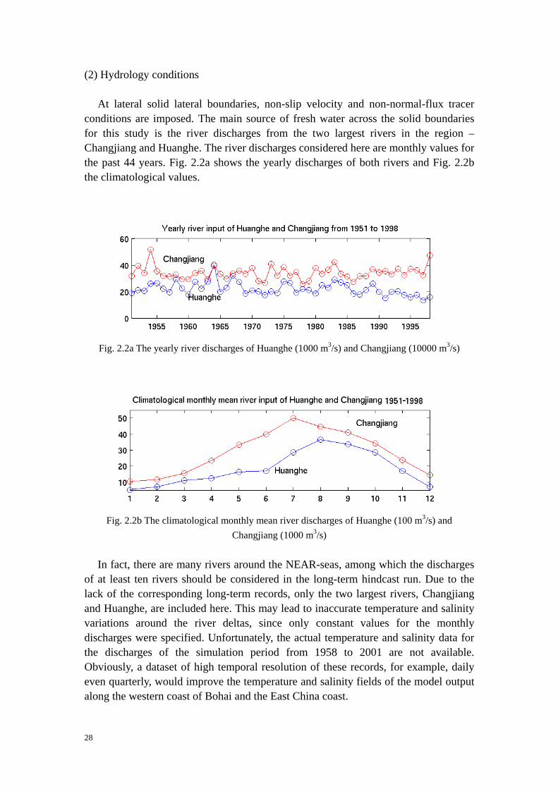
At lateral solid lateral boundaries, non-slip velocity and non-normal-flux tracer conditions are imposed. The main source of fresh water across the solid boundaries for this study is the river discharges from the two largest rivers in the region – Changjiang and Huanghe. The river discharges considered here are monthly values for the past 44 years. Fig. 2.2a shows the yearly discharges of both rivers and Fig. 2.2b the climatological values.

Fig. 2.2a The yearly river discharges of Huanghe (1000 m3/s) and Changjiang (10000 m3/s)

Fig. 2.2b The climatological monthly mean river discharges of Huanghe (100 m3/s) and Changjiang (1000 m3/s)

In fact, there are many rivers around the NEAR-seas, among which the discharges

of at least ten rivers should be considered in the long-term hindcast run. Due to the lack of the corresponding long-term records, only the two largest rivers, Changjiang and Huanghe, are included here. This may lead to inaccurate temperature and salinity variations around the river deltas, since only constant values for the monthly discharges were specified. Unfortunately, the actual temperature and salinity data for the discharges of the simulation period from 1958 to 2001 are not available. Obviously, a dataset of high temporal resolution of these records, for example, daily even quarterly, would improve the temperature and salinity fields of the model output along the western coast of Bohai and the East China coast.

28

At the ocean bottom where the flow is constrained to be parallel to the sea floor, a quadratic bottom stress with a drag coefficient of 2.5x10-3 is applied. There is no flux of heat or salt through the sea floor.

(3) Meteorological conditions

The ECMWF 40-year Re-analysis Data Archive (ERA-40) now covers the whole

period from September 1957 to August 2002. It provides a new potential for studying long-term trends and fluctuations such as ENSO and QBO in the global climate system. For this hindcast simulation, the heat flux, salt flux and locally imposed windstress as well as sea level pressure fields at the model surface are calculated from the quarterly ERA40 re-analysis dataset in order to examine the circulation driven by long-term climate changes. The heatflux through the sea surface is calculated by adding all heatflux components through the sea surface, with the help of bulk formulae (Schrum and Backhaus 1999), which determines the change of the heat content in the sea surface layer due to the atmospheric forcing. The meteorological parameters necessary for these bulk formulae such as wind stress, relative humidity, solar radiation and cloud cover are also calculated from the ERA40 re-analysis dataset. The parameters used here are listed below in table 2.1.

Table 2.1 Six-hourly surface flux parameters of the model input3

ERA40 ID Level Variable Unit 142 Surface Large scale precipitation m of water per second 143 Surface Convective precipitation m of water per second 151 Surface Mean sea level pressure Pascal 164 Surface Total cloud cover (0-1) 165 10 m U wind component m/s 166 10 m V wind component m/s 167 2 m Air Temperature K 168 2 m Dew point temperature K 176 Surface Surface solar radiation W/m2 182 Surface Evaporation m of water per second

2.2.2 Model initialization and modelling strategy

With the technical support from DKRZ (Deutsches KlimaRechenZentrum), the

HAMSOM model is modified to be capable of parallel run on the NEC SX-6 series multi-CPU vector supercomputers. For this study the well-tested parallelised HAMSOM model optimally needs 6-CPUs with one compute node specified.

A time step of ten minutes is used for the long-term model simulation. The

horizontal mixing coefficients of momentum, temperature and salinity in the model are set to the same constant value. Vertical mixing and viscosity are calculated by a level-2 Kochergin-Pohlmann scheme (Pohlmann 1996a). The model is initialized with the climatological monthly mean fields of temperature and salinity both in interior and

3 http://www.mad.zmaw.de/

29

at the lateral open boundaries (Levitus 1998), and then performs immediately a fully prognostic baroclinic run. The model calculates the hydro- and thermodynamic parameters continuously for the time period from 1 January 1958 to 31 December 2001.

For the first several days there is a completely absence of the Kuroshio front in the

temperature and salinity fields, suggesting a vigorous initial adjustment. The baroclinic velocity field is then derived from the initial temperature and salinity fields on the basis of the thermal wind relation. The barotropic velocity field is produced by the boundary sea level height. A realistic circulation pattern of the model field is quickly reached afterwards. The major spin-up occurs primarily in the first fifteen days.

The daily mean model outputs for the long-term 44-year simulation include

three-dimensional ocean temperature and salinity fields, the three-dimensional velocity and vertical viscosity fields, three-dimensional kinematic energy and two-dimensional sea surface elevation fields.

In the following chapters the verification and analysis of these daily outputs will be

discussed.

30

Chapter 3 Model validation

In this chapter, the long-term hindcast of HAMSOM model will be validated using the historical observations and the satellite remote sensing observations in NEAR-seas. The historical observations include the data derived from tide gauges, ocean temperature stations and ship cruises. The satellite data are composite of AVHRR Ocean Pathfinder sea surface temperature and the AVSIO absolute dynamic topography. 3.1 Historic observations of the NEAR-seas 3.1.1 Model validation using hourly sea level data

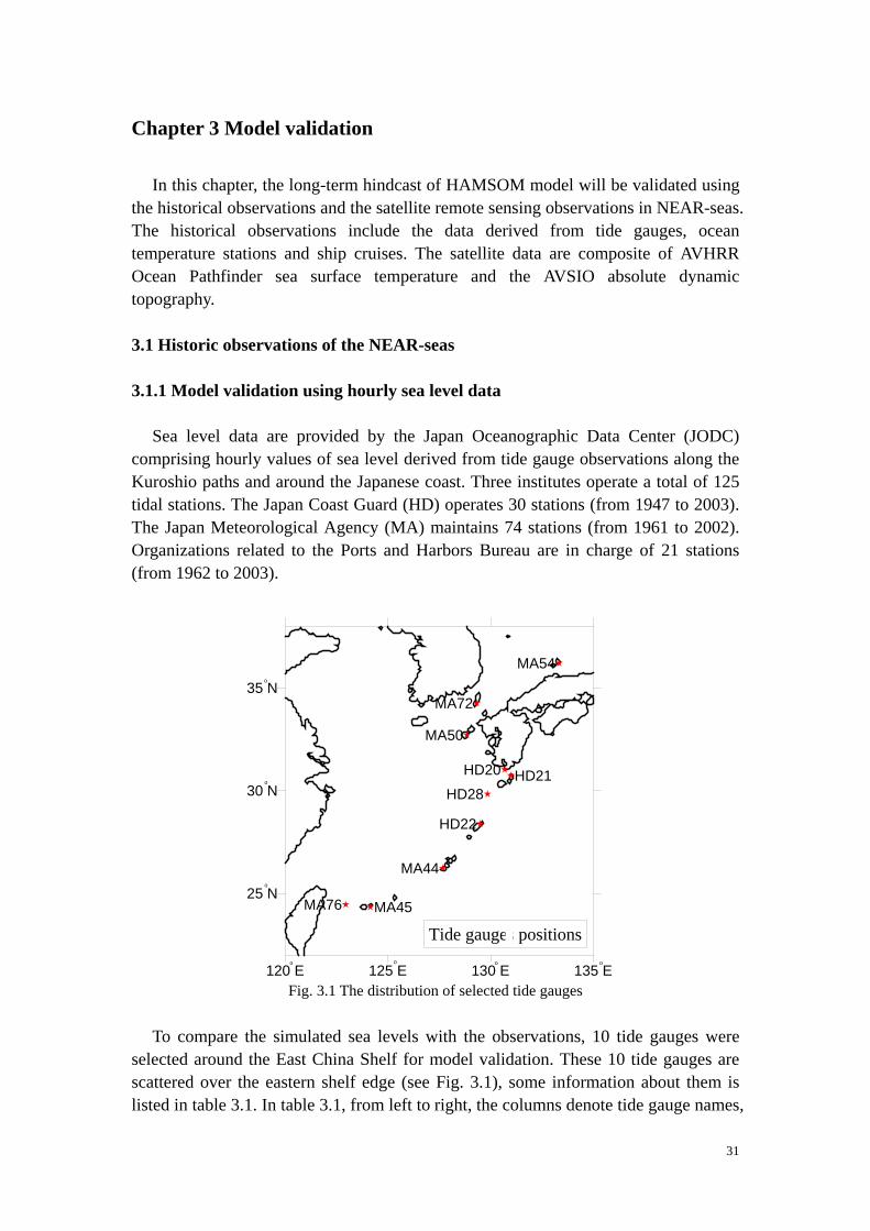
Sea level data are provided by the Japan Oceanographic Data Center (JODC) comprising hourly values of sea level derived from tide gauge observations along the Kuroshio paths and around the Japanese coast. Three institutes operate a total of 125 tidal stations. The Japan Coast Guard (HD) operates 30 stations (from 1947 to 2003). The Japan Meteorological Agency (MA) maintains 74 stations (from 1961 to 2002). Organizations related to the Ports and Harbors Bureau are in charge of 21 stations (from 1962 to 2003).

120 E 125 E 130 E 135 E

25 N

30 N

35 N

HD22

MA44

HD28

MA50

MA54

MA72

MA76

HD20

MA45

HD21

Tide gauges positions

o

o

o

o o o o

Fig. 3.1 The distribution of selected tide gauges To compare the simulated sea levels with the observations, 10 tide gauges were

selected around the East China Shelf for model validation. These 10 tide gauges are scattered over the eastern shelf edge (see Fig. 3.1), some information about them is listed in table 3.1. In table 3.1, from left to right, the columns denote tide gauge names,

31

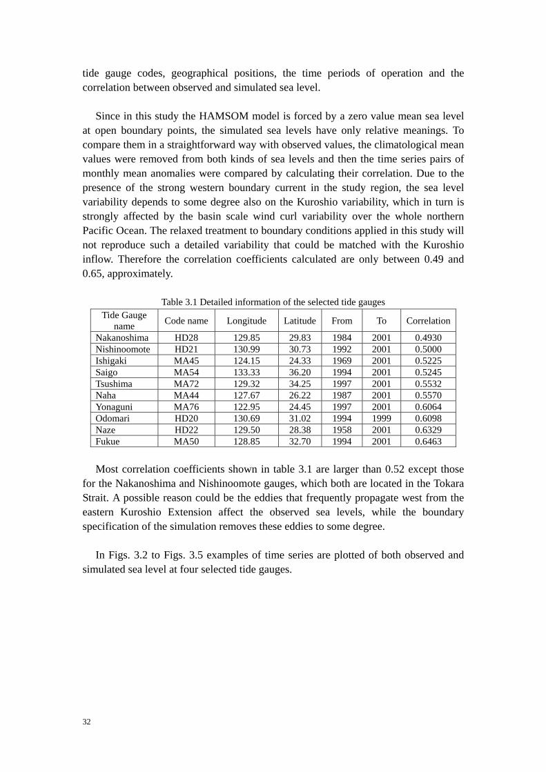
tide gauge codes, geographical positions, the time periods of operation and the correlation between observed and simulated sea level.

Since in this study the HAMSOM model is forced by a zero value mean sea level

at open boundary points, the simulated sea levels have only relative meanings. To compare them in a straightforward way with observed values, the climatological mean values were removed from both kinds of sea levels and then the time series pairs of monthly mean anomalies were compared by calculating their correlation. Due to the presence of the strong western boundary current in the study region, the sea level variability depends to some degree also on the Kuroshio variability, which in turn is strongly affected by the basin scale wind curl variability over the whole northern Pacific Ocean. The relaxed treatment to boundary conditions applied in this study will not reproduce such a detailed variability that could be matched with the Kuroshio inflow. Therefore the correlation coefficients calculated are only between 0.49 and 0.65, approximately.

Table 3.1 Detailed information of the selected tide gauges

Tide Gauge name Code name Longitude Latitude From To Correlation

Nakanoshima HD28 129.85 29.83 1984 2001 0.4930 Nishinoomote HD21 130.99 30.73 1992 2001 0.5000 Ishigaki MA45 124.15 24.33 1969 2001 0.5225 Saigo MA54 133.33 36.20 1994 2001 0.5245 Tsushima MA72 129.32 34.25 1997 2001 0.5532 Naha MA44 127.67 26.22 1987 2001 0.5570 Yonaguni MA76 122.95 24.45 1997 2001 0.6064 Odomari HD20 130.69 31.02 1994 1999 0.6098 Naze HD22 129.50 28.38 1958 2001 0.6329 Fukue MA50 128.85 32.70 1994 2001 0.6463 Most correlation coefficients shown in table 3.1 are larger than 0.52 except those

for the Nakanoshima and Nishinoomote gauges, which both are located in the Tokara Strait. A possible reason could be the eddies that frequently propagate west from the eastern Kuroshio Extension affect the observed sea levels, while the boundary specification of the simulation removes these eddies to some degree.

In Figs. 3.2 to Figs. 3.5 examples of time series are plotted of both observed and

simulated sea level at four selected tide gauges.

32

Fig. 3.2 A 44-year comparison at tide gauge Naze (line: observations, dots: simulated)

33

Fig. 3.3 A 33-year comparison at tide gauge Ishigaki (line: observations, dots: simulated)

34

Fig. 3.4 A 7-year comparison at tide gauge Fukue (line: observations, dots: simulated)

Fig. 3.5 A 5-year comparison at tide gauge Yonaguni (line: observations, dots: simulated)

35

3.1.2 Model validation using the temperature station data The Japan Meteorological Agency (JMA) has carried out oceanographic and

marine meteorological observations at the coastal water temperature observation stations, on board research vessels and on moored ocean buoys. Water temperature observations have been carried out by JMA at 21 stations along the Japanese coast since the early 1950s. The published temperature data include monthly mean and 10-day average temperatures until early 1995 or early 1999. Since April 1995, water temperature has been observed daily at 7 stations including Esashi, Omaezaki, Hachijojima, Hamada and Ishigaki. Hourly sampling has been done at the same 7 stations since April 1996.

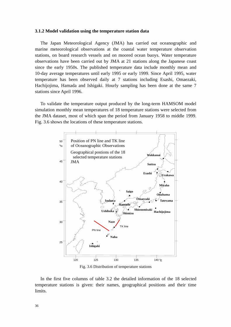
To validate the temperature output produced by the long-term HAMSOM model

simulation monthly mean temperatures of 18 temperature stations were selected from the JMA dataset, most of which span the period from January 1958 to middle 1999. Fig. 3.6 shows the locations of these temperature stations.

120 125 130 135 140

25

30

35

40

45

50

Wakkanai

Suttsu

UrakawaEsashi

Naha

Miyako

OnahamaOmaezaki Tateyama

Hachijojima

Saigo

Hamada

ShionomisakiShimizu

Izuhara

Ushibuka

Naze

Ishigaki

Geographical postions of the 18 selected temperature stationsJMA

Position of PN line and TK lineof Oceanographic Observations

PN lineTK line

oN

oE Fig. 3.6 Distribution of temperature stations

In the first five columns of table 3.2 the detailed information of the 18 selected

temperature stations is given: their names, geographical positions and their time limits.

36

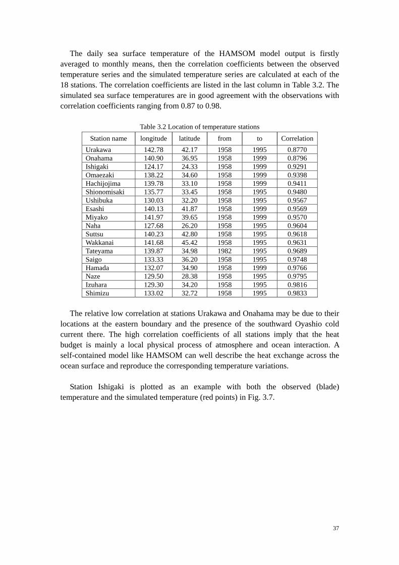
The daily sea surface temperature of the HAMSOM model output is firstly averaged to monthly means, then the correlation coefficients between the observed temperature series and the simulated temperature series are calculated at each of the 18 stations. The correlation coefficients are listed in the last column in Table 3.2. The simulated sea surface temperatures are in good agreement with the observations with correlation coefficients ranging from 0.87 to 0.98.

Table 3.2 Location of temperature stations

Station name longitude latitude from to Correlation Urakawa 142.78 42.17 1958 1995 0.8770 Onahama 140.90 36.95 1958 1999 0.8796 Ishigaki 124.17 24.33 1958 1999 0.9291 Omaezaki 138.22 34.60 1958 1999 0.9398 Hachijojima 139.78 33.10 1958 1999 0.9411 Shionomisaki 135.77 33.45 1958 1995 0.9480 Ushibuka 130.03 32.20 1958 1995 0.9567 Esashi 140.13 41.87 1958 1999 0.9569 Miyako 141.97 39.65 1958 1999 0.9570 Naha 127.68 26.20 1958 1995 0.9604 Suttsu 140.23 42.80 1958 1995 0.9618 Wakkanai 141.68 45.42 1958 1995 0.9631 Tateyama 139.87 34.98 1982 1995 0.9689 Saigo 133.33 36.20 1958 1995 0.9748 Hamada 132.07 34.90 1958 1999 0.9766 Naze 129.50 28.38 1958 1995 0.9795 Izuhara 129.30 34.20 1958 1995 0.9816 Shimizu 133.02 32.72 1958 1995 0.9833

The relative low correlation at stations Urakawa and Onahama may be due to their

locations at the eastern boundary and the presence of the southward Oyashio cold current there. The high correlation coefficients of all stations imply that the heat budget is mainly a local physical process of atmosphere and ocean interaction. A self-contained model like HAMSOM can well describe the heat exchange across the ocean surface and reproduce the corresponding temperature variations.

Station Ishigaki is plotted as an example with both the observed (blade)

temperature and the simulated temperature (red points) in Fig. 3.7.

37

Fig. 3.7 Temperature comparison at temperature station Ishigaki from 1958 to 1999 (line: observations, dots: simulated)

38

3.1.3 Model validation using oceanographic observations

From the 1970s, oceanographic observations on board research vessels have been conducted by JMA in waters adjacent to Japan and in the western North Pacific Ocean on six vessels. Two ship lines of oceanographic observations from 1995 and 1996, located on the East China Shelf are selected as a reference. These two lines are named PN and TK line, respectively. The positions of the ship lines are depicted in Fig. 3.6 (red lines) and information for these three selected cruises along the PN and TK lines is listed in table 3.3.

Table 3.3 Information about the corresponding cruises Ship line names Cruise time Start points End points

PN9506 July 19-27 1995 124.52oE 30.00oN 128.25oE 27.52oN PN9606 July 22-24 1996 128.23oE 27.53oN 124.50oE 30.00oN TK9506 August 7-8 1995 129.77oE 28.57oN 130.83oE 30.25oN

The cruises along the PN section lasted 9 and 13 days, the cruise along the TK

section lasted two days. To compare the observations with the simulated temperature and salinity fields the time in the middle of each cruise is specified as the model time for producing the figure.

Figs. 3.8, 3.9 and 3.10 show the observed and simulated temperature and salinity

distributions, respectively, along the PN section of cruise PN9606. The patterns of the simulated fields are in good agreement with those of the observed ones. Thermocline and halocline are found both in the simulated and observed fields. The maximum simulated surface temperature is 28oC. The simulated salinity field has a more focused salinity core over the shelf break than observational field.

Fig. 3.8 Temperature (a) and salinity (b) observations with depth (Units: meter) of cruises PN9606 (Product of JMA)

Figs. 3.11, 3.12 and 3.13 correspond to PN9506. The general patterns of the

observed and simulated fields are comparable. One difference is that the surface temperature of the western PN section was 1oC warmer than the simulated results. Maybe this is due to the daily averaging to the model result. The relatively flat halocline and thermocline in the simulated fields could be a result of the daily averaging of the model results.

39

Fig. 3.14 shows the section field of the simulated and of the observed temperature along TK9506, Fig. 3.15 is the same as Fig. 3.14 but for the salinity field.

Fig. 3.9 Simulated temperature of section PN9606

Fig. 3.10 Simulated salinity of section PN9606

40

Fig. 3.11 Simulated temperature of section PN9506

Fig. 3.12 Temperature observations of cruise PN9506 (JMA product)

41

Fig. 3.13a Simulated salinity of section PN9506

Fig. 3.13b Salinity observations of cruise PN9506 (JMA product)

42

Fig. 3.14a Simulated temperature of section TK9506

Fig. 3.14b Temperature observations of cruise TK9506 (JMA product)

43

Fig. 3.15a Simulated salinity of section TK9506

Fig. 3.15b Salinity observations of cruise TK9506 (JMA product)

44

3.2 Satellite remote sensing observations of the North East Asia Regional seas 3.2.1 Model validation using the AVHRR Oceans Pathfinder SST4

The NOAA/NASA AVHRR Oceans Pathfinder sea surface temperature data are

derived from the 5-channel Advanced Very High Resolution Radiometers (AVHRR) on board the NOAA -7, -9, -11, -14, -16 and -17 polar orbiting satellites. Monthly averaged data for both the ascending pass (daytime) and descending pass (nighttime) are cited here for the validation of the model runs. Since the resolution of the numeric model is 1/12 by 1/12 degrees, satellite data are selected that are produced on equal-angle grids of 4096 pixels/360 degrees which is nominally referred to as the 9 km resolution. Thus, the resolution of the remote sensing data and that of the simulated data of this study are compatible.

The simulated monthly mean SST is calculated by averaging the daily temperature

of the first model layer. For the monthly mean Pathfinder SST the average of their ascending pass and descending pass is calculated and used to compare with the simulation result.

The verification of the model surface temperature using the AVHRR SST is done

for the months of August 1992, October 1992, May 1993 and October 1997. Fig. 3.16 shows that the 28oC and 29oC contour lines in August of both fields are in good agreement, with one difference being a closed 29oC contour southwest of the Cheju Island, and another deviation is at the southeastern boundary. The general patterns coincide well, however.

In Figs. 3.17 a similar result of matching patterns can be seen, except for a little

northward intrusion of the 24oC contour line in the northern East China Sea and a deviation at the eastern boundary.

In May 1993 better agreement is found along the eastern model boundary, yet with

a slight northward expulsion of the 26oC temperature contour near the southern boundary (Fig. 3.18). The cold tongue-like temperature contours bend southeastward in the southern Huanghai and northern East China Sea, which can be seen in both the remote sensing field and the observed field.

4 http://podaac.jpl.nasa.gov/sst/

45

Fig. 3.16a Monthly mean satellite Pathfinder SST of Aug 1992 Fig. 3.16b Monthly mean simulated SST of Aug 1992

46

Fig. 3.17a Monthly mean satellite Pathfinder SST of Oct 1992 Fig. 3.17b Monthly mean simulated SST of Oct 1992

47

Fig. 3.18a Monthly mean satellite Pathfinder SST of May 1993 Fig. 3.18b Monthly mean simulated SST of May 1993

48

3.2.2 Model validation using the AVISO absolute dynamic topography5

AVISO France distributes satellite altimetry data from Topex/Poseidon, Jason-1,

ERS-1 and ERS-2, and EnviSat, and Doris precise orbit determination and positioning products. These data are used to study ocean dynamics and geophysics in many applications, including climate prediction, monitoring of mean sea level, global warming, El Niño and La Niña events, ocean currents and circulation, tides, wind, wave and marine meteorology models.

The absolute dynamic topography provided by AVISO is a result of sea surface

height due to mean currents plus variations of the sea surface height and is used for the study of the general circulation. Its resolution is 1/3°x1/3° given on a Mercator grid. The temporal resolution is one record for every seven days.

From the published absolute dynamic topography data (They begin on 24 August

2001), satellite data of two months in 2001 were selected for comparison with the long-term HAMSOM model simulations. These two months are September and November. First, the weekly absolute dynamic topography and the model-simulated daily sea levels are averaged to monthly mean values, without removing the mean sea level from the AVISO absolute dynamic topography. Thus, the verification made here is qualitatively rather than quantitatively.

In Figs. 3.19 the dense contour lines represent the Kuroshio in both fields from

September 2001. The low in sea level of the simulated field in the central East China Sea is deeper than in the remote sensing field. A maximum in absolute dynamic topography is seen only in the remote sensing field near the Chinese coast north of 30oN. Figs. 3.20 show the dynamic topography of December in 2001. Similar to the situation in September 2001, two warm eddies appear only in the remote sensing field along the China coast near 30oN. Another difference between the satellite and simulated field is the location of the Kuroshio paths south of Japan across 140oE. The Kuroshio paths in the East China Sea, however, are in good agreement.

From the above discussion follows that the boundary effects may strongly

influence the Kuroshio system, especially near the region of the Kuroshio Extension, made up of the Kuroshio and the accompanying eddy system. The westward propagating eddies are normally incited in the Kuroshio Extension and propagate westward to the east of the Tokara Strait, then they facilitate the trigger meander of the Kuroshio to induce the Kuroshio large meander south of Japan. The model, however, fails to reproduce this process in December 2001, and the ‘simulated’ Kuroshio does not deviate southward at 140oE. A possible reason is located in the inflow and outflow conditions which strongly affect the Kuroshio path south of Japan.

5 http://www-aviso.cls.fr/html/donnees/produits/madt_uk.html

49

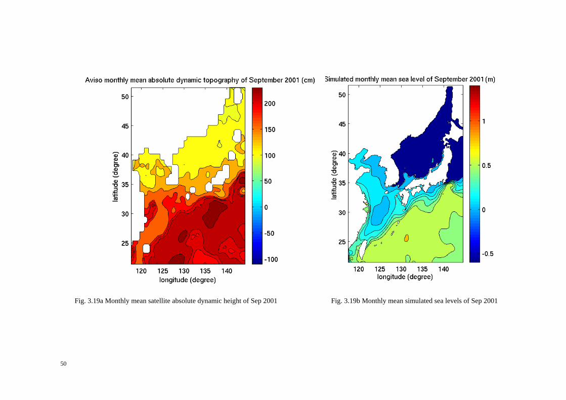
Fig. 3.19a Monthly mean satellite absolute dynamic height of Sep 2001 Fig. 3.19b Monthly mean simulated sea levels of Sep 2001

50

Fig. 3.20a Monthly mean satellite absolute dynamic height of Dec 2001 Fig. 3.20b Monthly mean simulated sea levels of Dec 2001

51

3.3 Summary

In this chapter the model was validated using historical tide gauge observations, temperature stations, sections of oceanic cruises and remote sensing fields. Several features of the model fields can be summarized as: a. The long-term variability of the simulated temperature fields is well reproduced in

most of the model domain, especially on the East China Shelf where the Kuroshio dominates. For some months, temperatures along the eastern model boundary are perturbed by the boundary effect. Along the southern boundary the temperature field matches the observations more closely. Obviously the well-reproduced temperature fields indicate that the sea surface temperature is mainly determined by the local physical processes of ocean atmosphere interaction.

b. Although no validation is made for the salinity field due to lack of observations, an

under-estimated salinity field can be expected since the discharges of the two largest rivers considered are taken as pure fresh water in the model.

c. The high correlation between the observed and simulated sea level fields indicates

that the boundary conditions for the regional model of NEAR-seas are particularly important because of the through-flow of the Kuroshio in the region. As one of the two strongest western boundary currents in the world ocean, the Kuroshio dominates the current fields over the whole eastern and northern China Shelf. A realistic inflow prescribed at the southern boundary and outflow at the eastern boundary is prone to improve the sea level field of the NEAR-seas.

Summarizing: The long-term simulation described in the previous chapters

reproduces a plausible variability field at least along the Kuroshio paths on the East China Shelf. The model output can therefore be used to study local physical oceanic problems and long-term variations of related oceanographic variables.

52

Chapter 4 The Drifter field 4.1 The WOCE SVP program

The Surface Velocity Programme (SVP) of WOCE (World Ocean Circulation Experiment) was developed as a partnership between the Global Drifter Center (GDC) located at the Atlantic Oceanographic and Meteorological Laboratory (AOML) in Miami, USA, and the Marine Environmental Data Service (MEDS) of the Canadian Department of Fisheries and Oceans in Ottawa. The program started with the release of Global Langrangian Drifters by volunteer ships in 1979.

Normally the drifter consists of a 15m holey-sock drogue and a sensor attachment.

Both parts together have a length of 18m at depth. The drogues are designed to accurately depict ocean currents by avoiding sensor susceptibility due to wave and wind action. The drifters transmit sensor data to satellites that determine the buoy’s position and relay the data to Argos ground stations. Thus, the data records include the time dependent location of the buoy and oceanographic variables such as air pressure, sea surface temperature, sea surface salinity and wind data. AOML handles the initial processing of the data received through Service Argos. They carry out quality control of the data, generate the interpolated KRIG6 file and forward the data to MEDS which functions as the archive center. The KRIG data is then quality controlled and optimally interpolated to uniform six-hour interval trajectories for archival at MEDS (Hansen and Poulain 1996).

The SVP program made it possible to study general ocean circulation patterns and

the interaction between oceanic areas and shelf seas in a Langrangian way. Fig. 4.1.1 shows velocity averages in the Pacific Ocean for the month of February 2000. The data are averaged over five day intervals into 5 degree by 5 degree bins.

Fig. 4.1.1 The mean velocity averages of the Pacific Ocean in February 2000

In Fig. 4.1.1 the surface equatorial current system is well reproduced. Although there are not enough buoys deployed in the research area in February 2000, the large 6 KRIG is the name of the quarter (six hourly) file of the satellite-traced buoys.

53

velocity amplitude east of Taiwan Island, over the East China Shelf edge and south of Japan is striking. 4.2 Buoys released in North East Asian Regional seas

The first buoy entering the North East Asian Regional (NEAR) seas was released in the year of 1989, with an objective to study the Kuroshio path. For the purpose of this study, i.e. to investigate the surface velocity field using drifter data, all KRIG data for 11 years from 1989 to 1999 were collected. A total of 661 Global Langrangian Drifters appeared in the NEAR region. Focus on the Kuroshio dynamics, a dataset composing of only 250 buoys was selected. Fig. 4.2.1 shows the spatial distribution of the starting points of those buoys. Here the start point means the position where the first available data record after the buoy appeared in the NEAR-seas.

According to different objectives, these buoys were mainly deployed in three areas:

around Taiwan Island (Area A, 115 buoys), over the East China Shelf near 30oN (Area B, 52 buoys) and in the Japan Sea west of 135oE (Area C, 49 buoys). The other 34 buoys are scattered in the eastern Japan Sea (4 buoys), east of the Ryukyu archipelago (10 buoys) and near the central southern boundary of the study region (20 buoys).

120 125 130 135 140

25

30

35

40

45

50

20

76

Aear B 52

25

Aear C 49

99

31

The spatial distribution of start points of the SVP global lagrangian drifters( 1989 - 1999 )

Area A 115

CHINA

KOREA

JAPAN

oE

oN

Fig. 4.2.1 The spatial release points distribution of the 250 buoys.

The distribution of the buoy starting points obviously emphasizes the variability of the Kuroshio path, of the cross shelf currents and of the Tsushima Current, which is one main research topic of the SVP program. Fig. 4.2.2 indicates the temporal distribution of the number of released buoys. Panel a) shows release peaks in 1992,

54

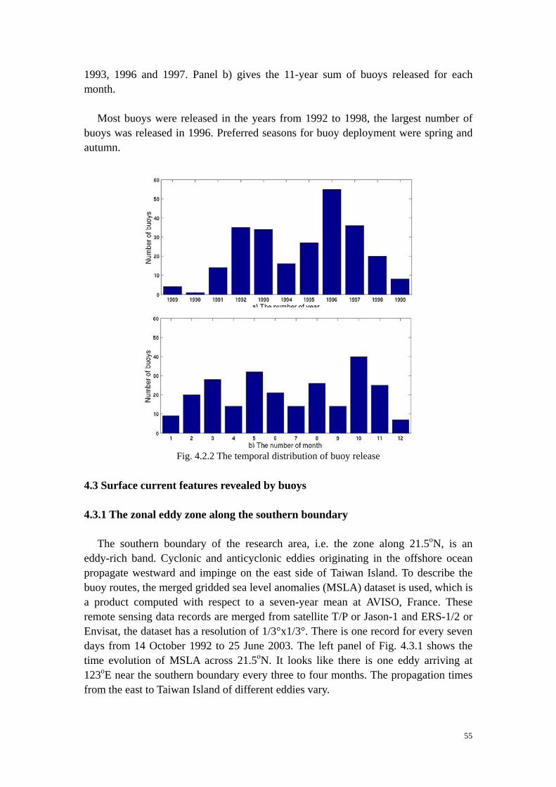
1993, 1996 and 1997. Panel b) gives the 11-year sum of buoys released for each month.

Most buoys were released in the years from 1992 to 1998, the largest number of

buoys was released in 1996. Preferred seasons for buoy deployment were spring and autumn.

Fig. 4.2.2 The temporal distribution of buoy release 4.3 Surface current features revealed by buoys 4.3.1 The zonal eddy zone along the southern boundary

The southern boundary of the research area, i.e. the zone along 21.5oN, is an eddy-rich band. Cyclonic and anticyclonic eddies originating in the offshore ocean propagate westward and impinge on the east side of Taiwan Island. To describe the buoy routes, the merged gridded sea level anomalies (MSLA) dataset is used, which is a product computed with respect to a seven-year mean at AVISO, France. These remote sensing data records are merged from satellite T/P or Jason-1 and ERS-1/2 or Envisat, the dataset has a resolution of 1/3°x1/3°. There is one record for every seven days from 14 October 1992 to 25 June 2003. The left panel of Fig. 4.3.1 shows the time evolution of MSLA across 21.5oN. It looks like there is one eddy arriving at 123oE near the southern boundary every three to four months. The propagation times from the east to Taiwan Island of different eddies vary.

55

For example, a cyclonic eddy appears at the southern boundary near 142oE on 14 October 1992 and propagates westward to 122.5oE on 22 June 1993. Another example is three anticyclonic eddies arriving at the southern boundary near 126oE, 137.5oE and 142.5oE on 27 May 1995 and propagating westward, the central eddy arrived at 123oE on 15 November 1993. The right panel of Fig. 4.3.1 is the same as the left panel but along latitude 24.3oN, these westward propagating eddies are also evident for this latitude. The panels of Fig. 4.3.1 therefore depict a band of westward propagating eddies between 21.5oN and 24.3oN.

In Figs. 4.3.2 and 4.3.3, four meridional sections are presented. The zonal

eddy-rich band south of 25oN is seen across 124oE, 127.3oE and 130oE. These eddies weaken as they propagate westward and finally merge with the western boundary current – the Kuroshio. The upper panel of Fig. 4.3.3 along 130oE suggests that the Tsushima Strait and the Tokara Strait are also eddy-rich areas.

The lower panel in Fig. 4.3.3 shows the sea level evolution along the eastern model

boundary (144.5oE) and no eddies appear in the south but the Kuroshio displays a meridional shift, the center is located at 34oN.

Fig. 4.3.4 gives the trajectory of Buoy 9523909 following the anticyclonic eddy

formed in May 1995 which is mentioned above. On 13 August, the buoy started at 133.8oE, in November it arrived east of Taiwan Island. At the end of November 1995, the buoy joined the Kuroshio and drifted into the East China Sea. The sea level anomaly time series of the MSLA dataset proved the existence of the central eddy and its propagation, Fig. 4.3.5 gives a snapshot of that eddy on 11 December 1995, when it approached Taiwan Island from the southeast.

4.3.2 The current pattern northeast of Taiwan Island Northeast of Taiwan Island the Kuroshio runs across a nearly zonal shelf break.

The Kuroshio subsurface water upwells onto the shelf as the Kuroshio branches and the main current deflects seaward. Part of the branch current flows northward into the inner shelf and returns to the main Kuroshio stream. The other part forms cyclonic eddies at the northern tip of Taiwan Island. Figs. 4.3.6, 4.3.7 and 4.3.8 show some buoy tracks which documenting this branching and the current pattern there. The trajectories of most buoys deflect at the northeast of Taiwan Island towards the east. Some run onto the shelf, such as Buoy 7708706 in panel a) of Fig. 4.3.6, Buoy 9320608 in panel c), Buoy 7700524 in panel d) of the same figure, Buoy 9421972 in panel a) of Fig. 4.3.7, Buoy 9421985 in panel d) of this figure and Buoy 9421965 in Fig. 4.3.8a. In panel b) of Fig. 4.3.6b, Buoy 7700508 drifts onto the central East China Shelf and describes a cyclonic eddy there.

The buoy indicated by the red line in panel a) of Fig. 4.3.7 shows the cyclonic eddy

near the north coast of Taiwan Island. Fig. 4.3.8b is an enlarged figure of the buoy

56

trajectories north of Taiwan Island shown in Fig. 4.3.8a. The six buoys deployed on 5 October 1995 show a typical branching structure of the current field northeast of Taiwan Island. Buoys 9421963, 9421966 and 9421967 depict the cyclonic circulation near the north coast of Taiwan Island again.

Fig. 4.3.6a also indicates that the direction of the Taiwan Strait Current was

southward in October 1989 and in November 1991. Buoy 7708706 drifted southwestward from the beginning of October and into the South China Sea at the end of the same month. From late January to late March in 1993, Buoy 7700524 drifted from Taiwan Strait towards Tsushima Strait.

An interesting feature of the Kuroshio is presented in panel c) of Fig. 4.3.7. The

Kuroshio main stream deflects to the east near the central eastern coast of Taiwan Island. As discussed in section 4.3.1, this may be induced by an arrival of a westward propagating cyclonic eddy from the ocean’s interior.

4.3.3 The frontal eddies accompanying the Kuroshio in the East China Sea In Figs. 4.3.6 and 4.3.7 most buoys drift along irregular paths towards northeast to

the Tokara Strait. This can be seen more clearly in Figs. 4.3.9a and 4.3.9b. For example, Buoy 7714979 (red, Fig. 4.3.9a) swirls anticyclonically southwest of Tokara Strait from 15 October 1991 to 13 February 1992. Buoy 7714988 plotted in pink in Fig. 4.3.9b performs an anticyclonic motion in the same area.

4.3.4 Anticyclonic motions southwest of Kyushu and branching of the

Kuroshio there Near the area centered at 128oE and 31oN, the Kuroshio exhibits another branch

current, which is thought to be the source of the Huanghai or Tsushima Warm Current. Most part of this branch current forms an anticyclonic path back to the Kuroshio into the Tokara Strait. Some buoys in Fig. 4.3.10 indicate this anticyclonic motion.

The branching of the Kuroshio into Tsushima Strait can be seen in Figs. 4.3.11a to

Figs. 4.3.11e. Most buoys from the area near 128oE and 30oN drifted towards the Tsushima Strait. Some buoys drifted towards southwest of Cheju Island, such as Buoy 9619381 in Fig. 4.3.11b. The drifter paths shown in Fig. 4.3.11 suggest a division of the current into two classes by the obstacle of Tsushima Island. All buoys crossing the Tsushima Strait drifted further along the Japanese coast but the buoys that had crossed Korea Strait drifted northward along the eastern Korean coast.

57

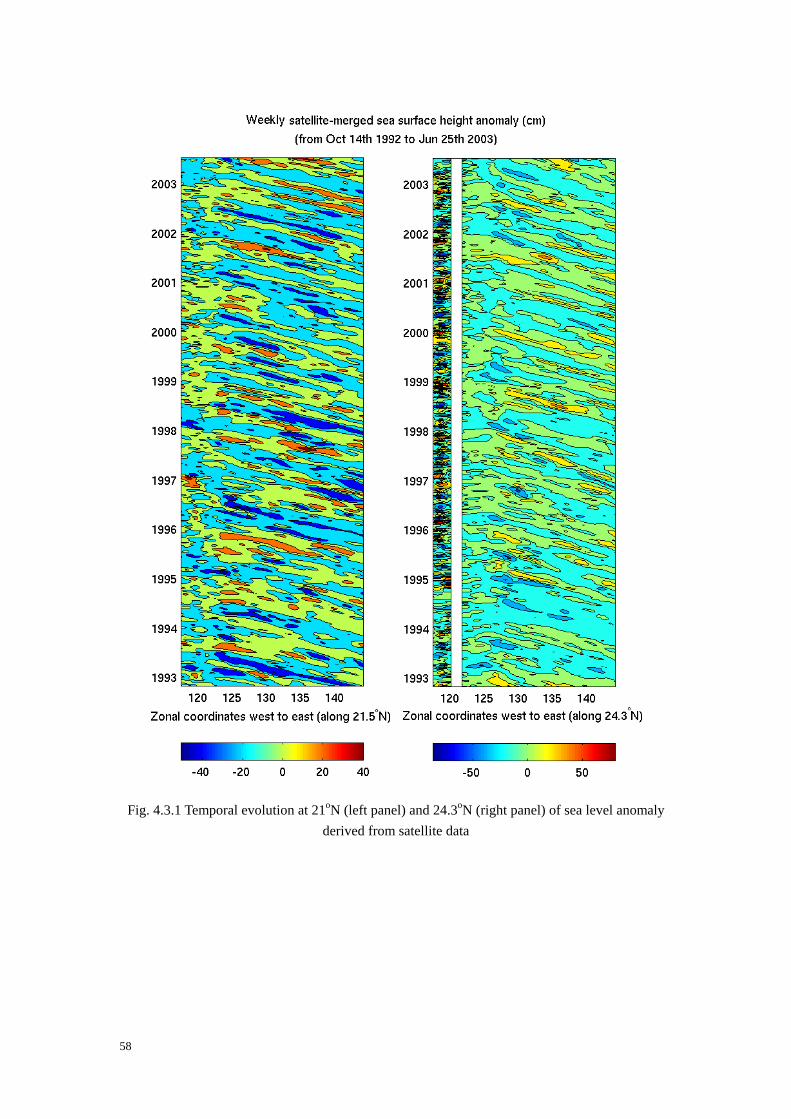
Fig. 4.3.1 Temporal evolution at 21oN (left panel) and 24.3oN (right panel) of sea level anomaly derived from satellite data

58

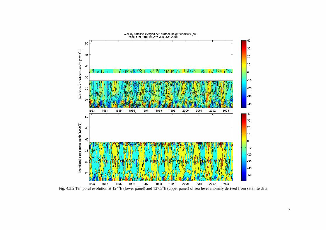
Fig. 4.3.2 Temporal evolution at 124oE (lower panel) and 127.3oE (upper panel) of sea level anomaly derived from satellite data

59

Fig. 4.3.3 Temporal evolution at 144.5oE (lower panel) and 130oE (upper panel) of sea level anomaly derived from satellite data

60

120 125 130

25

30

950803950831950928951026

951123

951221

Buoy 9523909

oN

oE

Fig. 4.3.4 Loops in the path of satellite drifting Buoy 9523909 Fig. 4.3.5 Satellite derived sea level anomaly on 11 Dec 1995

61

Fig. 4.3.6 The selected buoys that describe the current pattern around the Taiwan Island (The released date in the lower two panels is in 1992 and 1993, respectively)

120 125 130

25

30

920716920730

921008

921022921105921119

B7700503 RB7700506 GB7700504 BB7700508 PJul 15th 1992

120 125 130

25

30

930108

930122930205

930219930305930319

930402

B7700523 RB7700524 GB7700525 BJan 08th 1993

oE oE

oE oE 120 125 130

25

30

890903

890910

890917890924891001

891008

891015

891022 B7710570 Blu 890321

B7708706 Red

B7710802 Gre 890323B7714987 Pin 911101

120 125 130

25

30

red B9320608 931015pink B9619783 970920green B9619785 970921black B9727904 971010blue B0019790 971225

(c)(a) oN oN

(b) (d)

oN oN

62

120 125 130

25

30

941118

941230950210

941118

941230

950210

Fig. 4.3.7 Selected buoys describing the current pattern around Taiwan Island

941119

941203

Six buoys deployedon Nov 18th 1994

120 125 130

25

30

950305

950319950402

950416950430950514

B9320619B9421199B9421201March 5th 1995

o o

(c)(a) oN oN

oE oE

N

120 125 130

25

30N

960306960314

960322960330960407

960307

960318

960329960501

960512

Mar 07th 1996

B9421979 PinB9421976 BlaB9421972 Red

120 125 130

25

30

960512

960518960524

960514960519960524

960529960603

960608960613

B9421985

May 12th 1996

B9521984

(d)

oE oE

(b)

63

120oE 125oE 130oE

25oN

30oN

951005

951016

951027951104

951204951017

951005

951020951104

951026

951116

9421962 Pin9421963 Bla9421964 Gre9421965 Red9421966 Blu9421967 Pur

Oct 05th 1995

Fig. 4.3.8a Some buoys that describe the eddy over northern Taiwan Island shelf (Starting time is on 5 October 1995)

1 2 1 oE 1 2 1 .5 oE 1 2 2 oE 1 2 2 .5 oE

2 5 . 0 oN

2 5 . 5 oN

2 6 . 0 oN

2 6 . 5 oN

1 0 /1 6

1 0 /2 7

11 /0 4

1 2 /0 4

1 0 /1 6 1 0 /1 4

Fig. 4.3.8b The enlarged pictures of the buoys in Fig. 4.3.8a (time intervals of connecting arrows: one day)

64

120oE 125oE 130oE 135oE 140oE

25 oN

30 oN

35 oN

Fig. 4.3.9a Selected buoys that describe the Kuroshio frontal eddies

120oE 125oE 130oE 135oE 140oE

25 oN

30 oN

35 oN

Fig. 4.3.9b Selected buoys that describe the Kuroshio frontal eddies

25 oN

30 oN

35 oN

120oE 125oE 130oE 135oE 140oE

China

Korea

Kyushu

Fig. 4.3.10 The anticyclonic motions of the Kuroshio southwest of Kyushu

65

Fig. 4.3.11a Selected buoys that indicate the Kuroshio branching current

Fig. 4.3.11b Selected buoys that indicate the Kuroshio branching current

Fig. 4.3.11c Selected buoys that indicate the Kuroshio branching current

66

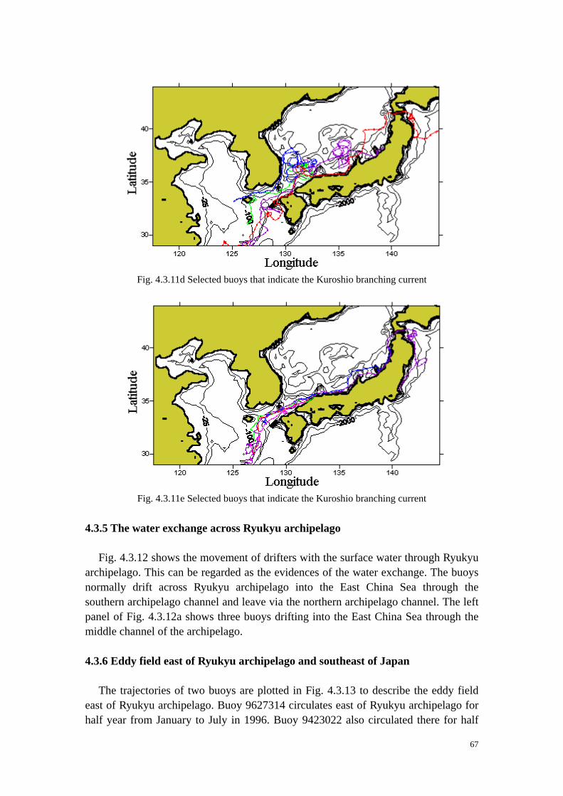
Fig. 4.3.11d Selected buoys that indicate the Kuroshio branching current

Fig. 4.3.11e Selected buoys that indicate the Kuroshio branching current 4.3.5 The water exchange across Ryukyu archipelago

Fig. 4.3.12 shows the movement of drifters with the surface water through Ryukyu archipelago. This can be regarded as the evidences of the water exchange. The buoys normally drift across Ryukyu archipelago into the East China Sea through the southern archipelago channel and leave via the northern archipelago channel. The left panel of Fig. 4.3.12a shows three buoys drifting into the East China Sea through the middle channel of the archipelago. 4.3.6 Eddy field east of Ryukyu archipelago and southeast of Japan

The trajectories of two buoys are plotted in Fig. 4.3.13 to describe the eddy field east of Ryukyu archipelago. Buoy 9627314 circulates east of Ryukyu archipelago for half year from January to July in 1996. Buoy 9423022 also circulated there for half

67

year in 1995. They appear to be trapped in an eddy field there. Summarizing the analysis of the drifter tracks shown in Fig. 4.3.9a an eddy system

is located south of Japan combined with the Kuroshio Extension. The eddy occurs normally on both sides of the Kuroshio Extension. The buoy trajectory in red in the same figure suggests a recirculation southwest of the Tokara Strait.

Fig. 4.3.12a Selected buoys indicate exchange crossing Ryukyu archipelago

Fig. 4.3.12b Selected buoys indicate exchange crossing Ryukyu archipelago

Fig. 4.3.13 Selected buoys indicate exchange crossing Ryukyu archipelago (right: B9423022)

68

4.4 The tracer model and the numerically produced tracer field

In order to both validate the current field of HAMSOM and reproduce the Langrangian trajectory pattern of released particles induced by the 3-dimensional velocity and diffusion field extracted from HAMSOM, a Langrangian tracer model is designed. The tracer model includes the horizontal and vertical diffusion effect by a random walk method (Monte-Carlo-Technique).

The tracer model interpolates the extracted daily velocity into short time steps

comparable with the tracer simulation, that means, over 24 hours the tracer will vary with the spatially temporally dependent velocity. Fig. 4.4.1 describes the drift of a tracer located in a 3-dimensional model grid cell moving into a neighboring grid cell within two time steps. In time step n, the tracer arrives at the point indicated by (Xn,Yn,Zn) which is located in the left model cell, the speed at that point will be calculated by interpolating the velocity values of the 8 corner points of the left model cell if they are wet points. For a dry corner point, the velocity at that point will not be considered. With this interpolated velocity Vn, the new position of the particle will be determined, i.e. the point indicated by (Xn+1,Yn+1,Zn+1) in Fig. 4.4.1, which is located in the right model cell.

For each time step after the displacement due to pure 3-dimensional velocity

forcing is determined, a displacement simulated by a Monte-Carlo-Technique representing the effect of 3-dimensional diffusion will be added. Then the final position of the tracer is given.

Fig. 4.4.1 Scheme of a tracer moving across model grid

(i,k-1,j) (i,k,j) (i,k+1,j)

(i,k,j+1)

(i+1,k+1,j+1)(i+1,k,j+1)

(i+1,k-1,j)

(Xn+1,Yn+1,Zn+1(Xn,Yn,Zn)

(i+1,k-1,j+1)

Since the Global Langrangian Drifters are drogued at about 18m depth, their

velocity corresponding to the two uppermost layers of this model, both of which are 10m thick. Considering that the buoys are generally drogued at this constant, near-surface depth only the horizontal velocity and diffusion fields are considered as forcing here. Thus the Global Langrangian Drifters will be thought of as a particle released at 10m depth, i.e. at the interface between the two uppermost model layers. The reason to include a random walk method is to simulate the tracer’s path in the most natural way possible, including the effect of diffusion.

69

As a numerical experiment of the tracer trajectory simulation, 70 particles are released at the same location near the eastern coast of Taiwan Island and their trajectories are calculated. The horizontal forcing velocity and diffusion fields are daily values of one particular month, i.e. May 1995. The forcing data are repeated during a 360-day simulation. Fig. 4.4.2 shows the contrast of the particles trajectory simulation with and without applying the walk method. In the left panel, the paths of all 70 particles are exactly the same (without random walk), while in the right panel the paths are spread out in a reasonable manner (with random walk).

Fig. 4.4.2 Contrast of the tracer trajectory simulation with (right) and without random walk (left)

As another example, with a zero diffusion value specified all 115 buoys that were released around Taiwan Island from 1989 to 1999 are simulated with the corresponding model generated horizontal velocity field. Here the zero diffusion also means that the random walk is disabled, thus in the figure each line stands for one buoy. The resulting distribution of these 115 buoys is shown in Fig. 4.4.3. In this figure, the color transition from red to blue means buoys’ deployments starting from 1989 and ending in 1999. A meander path and a jet-like path of the Kuroshio south of Japan are also developing according to Fig. 4.4.3.

In the following sections the simulation of the trajectories of the buoys released at

eastern Taiwan Island coast, released over the East China Shelf and released in the Tsushima Strait will be described, respectively.

70

Fig. 4.4.3 A simulated pattern of all the 115 buoys without diffusion 4.4.1 Simulation of buoys released near the eastern Taiwan Island coast

From observations it is known that the Kuroshio flows into the East China Sea along the eastern Taiwan Island coast and bifurcates there. The trajectories of the SVP buoys confirm the Kuroshio bifurcation and other flow patterns in this region. To reproduce the corresponding flow field using the tracer model, some buoys are selected for the trajectory simulation here. Five buoys were released east of Taiwan Island simultaneously in early May 1992 by WOCE/SVP. Table 4.1 gives the information about these five buoys. Fig. 4.4.4 plots out the corresponding satellite monitored trajectories.

Table 4.1 Information on buoys released on 4 May 1992 Buoy

number longitude latitude Release

date Vanishing

date Survival

days 7700498 121.61 23.24 1992 05 04 921211 222 7700499 121.53 22.97 1992 05 04 921231 242 7700500 121.61 23.09 1992 05 04 920605 033 7700501 121.89 22.39 1992 05 04 920923 143 7700502 121.89 22.37 1992 05 04 921216 227

Note: Buoy 7700499 turned southward on 4 June 1996 and out of the research area at the southern boundary on 21 October. Buoy 7700501 drifted eastward out of the research area on 17 June 1996 and followed the eddy there for nearly three months, and finally drifted eastward on 9 September.

71

To numerically reproduce the routes of these five buoys, the velocity and diffusion fields of the same time period produced by the HAMSOM model are used to force the tracer model. The particles are released at the same time, a zero value diffusion and a value of 500 cm2/sec are used, respectively, where the latter value is that used in the HAMSOM model for momentum exchange.

Fig. 4.4.6 shows the simulated trajectories of these five buoys with a zero value for diffusion. It is interesting to find that there are two buoys that deviate from their observed paths onto the East China Shelf. The other three buoys repeat nearly the same path as observed. This means, sometimes, forcing due to pure horizontal advection does not give the full reality.

With the horizontal diffusion considered by means of the random walk method the

Buoy 7700500 was simulated by 100 particles released at the same point same date. Fig. 4.4.7 shows the simulated paths of that buoy. Fig. 4.4.8 and Fig. 4.4.9 show the simulated paths of Buoys 7700498 and 7700501, respectively.

On 24 August 1998, another nine buoys were released east of Taiwan Island by

WOCE/SVP. Table 4.2 gives their information and Fig. 4.4.5 shows their satellite returned trajectories. The satellite returned trajectories imply again that in the East China Sea the SVP buoys tightly follow the Kuroshio path and can be regarded as good tracers of the Kuroshio and its branch currents. With the method discussed above two buoys of this set of nine are simulated, and the results are plotted in Fig. 4.4.10 and Fig. 4.4.11.

Judging from their distribution pattern these simulated trajectories are in good

agreement with the satellite returned distribution. On the one hand the Kuroshio path is again reproduced using the tracer model, on the other hand the simulation of the released buoys near Taiwan Island coast confirms that the HAMSOM model displays a good performance in the NEAR-seas simulation.

In August 1996, the bifurcation of the Tsushima Current and the Huanghai Warm

Current from the Kuroshio can also be found in Fig. 4.4.10 and Fig. 4.4.11.

Table 4.2 Information on buoys released on 24 Aug 1996 Buoy

number Longitude Latitude Release

date Vanishing

date Survival

days 9525136 121.62 22.82 960824 961010 048 9525137 121.52 22.95 960824 961231 130 9525138 121.53 22.85 960824 961014 052 9525139 121.61 23 960824 970120 150 9525141 121.62 22.97 960824 961221 120 9525142 121.51 22.82 960824 961231 130 9525143 121.54 22.73 960824 961120 089 9525144 121.63 22.95 960824 970625 194 9525145 121.67 22.72 960824 961121 090

72

(No)

Fig. 4.4.4 The satellite traced routes of the buoys released in May 1992

Fig. 4.4.5 The satellite traced routes of the buoys released on 24 August 1996

(Eo) 120 125 130 135 140

25

30

35

40

45

50

7700502 start at 1992 05 04

7700498 start at 1992 05 04

7700500 start at 1992 05 04

The 5 buoys released in May 1992near the east coast of island Taiwan

7700501 start at 1992 05 04

7700499 start at 1992 05 04

(No)

(Eo) 120 125 130 135 140

25

30

35

40

45

50

9525136 start at 1996 089525137 start at 1996 089525138 start at 1996 089525139 start at 1996 089525141 start at 1996 089525142 start at 1996 089525143 start at 1996 089525144 start at 1996 089525145 start at 1996 08

The 9 buoys released in August 1996

near the east coast of island Taiwan

73

Fig. 4.4.6 Simulated trajectories of the five buoys with a zero diffusion value

Fig. 4.4.7 Simulated paths distribution of Buoy 7700500

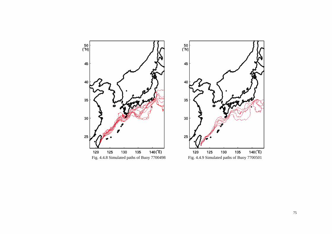
Fig. 4.4.8 Simulated paths of Buoy 7700498 Fig. 4.4.9 Simulated paths of Buoy 7700501

75

Fig. 4.4.10 Simulated paths of Buoy 9525138 Fig. 4.4.11 Simulated paths of Buoy 9525143

76

4.4.2 Simulation of buoys released over the East China Shelf

The shelf area near 126oE to 128oE and 30oN is an important research area for investigation of the Kuroshio branching phenomenon. Earlier studies suggest that the Kuroshio branching current supplies the water to Huanghai Warm Current and the Tsushima Warm Current at this location. To investigate the Kuroshio branching in this area, in 1998 a number of buoys were deployed over the central China shelf which is thought to be crucial for the origin of the Tsushima Warm Current and the Huanghai Warm Current. Fig. 4.4.12 shows the satellite-recorded routes of nine buoys which were deployed in 1998, their detailed information is listed in table 4.3.

Table 4.3 Information on buoys released in May 1998 Buoy

number longitude latitude Release

date Vanishing

date Survival

days 9619806 126.38 29.38 980429 980831 89 9715368 125.56 29.98 980429 980625 58 9715369 125.74 29.91 980430 980603 35 9715370 126.71 29.64 980430 980627 59 9730614 126.39 29.17 980501 980611 42 9730616 127.18 29.53 980501 980608 39 9730617 127.56 29.43 980501 980714 75 9721219 126.1 32.9 980502 980510 9 9721218 125.94 31.86 980503 980613 42

To simulate these nine buoys, they are first driven purely by advection. After that

two of them are studied using the random walk method. Fig. 4.4.13 shows the simulated routes of all nine buoys without horizontal

diffusion. This figure documents that the tracer model embedded in HAMSOM well reproduces the observed buoy trajectories shown in Fig. 4.4.12.

Fig. 4.4.14 is a composite display of 24 simulated trajectories of particles released

at the same point and the same time as Buoy 9715368. After some time, seven of them turn southeastward, pass through the northern Tokara Strait and follow the Kuroshio to the northeast. Three of them drift southwestward along the Chinese coast up to northern Taiwan Strait. This means that with random walk considered these 24 particles started from the central East China Shelf first may drift any direction, but their final destinations are obviously determined by the forcing current field. The three southward particles imply the southward coastal current along the east China coast in winter. The seven particles swirling southeastward imply the water is anticyclonic motion west of Kyushu.

Fig. 4.4.15 is a composite display of 37 simulated trajectories of particles released

at the same point and the same time as Buoy 9721219. All these particles go directly to Tsushima Island and into the Japan Sea. Most of them disperse along the Japanese coast and six particles move through the Soya Strait. A few of them follow the East

Korean Coast Current (EKCC). It should be noticed here that most particles crossing the Korea Strait follow the EKCC, while those that passed through the Tsushima Strait headed northern coast of Japan. This phenomenon is also seen in Fig. 4.4.14.

(No)

(No)

120 125 130 135 140

25

30

35

40

45

50

9619806p.dat 9804299715368p.dat 9804299715369p.dat 9804309715370p.dat 9804309730614p.dat 9805019730616p.dat 9805019730617p.dat 9805019721219p.dat 9805029721218p.dat 980503

Fig. 4.4.12 The satellite-recorded routes of all nine buoys

Fig. 4.4.13 The simulated routes of all nine buoys

78

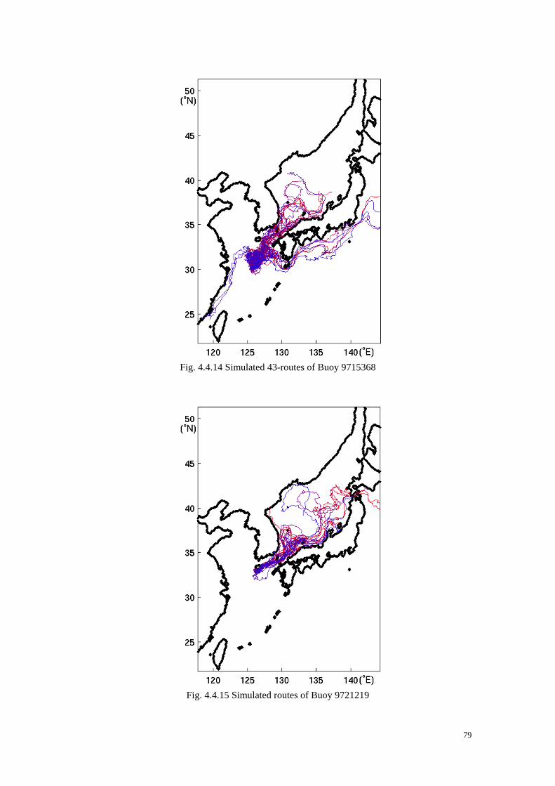
Fig. 4.4.14 Simulated 43-routes of Buoy 9715368

Fig. 4.4.15 Simulated routes of Buoy 9721219

79

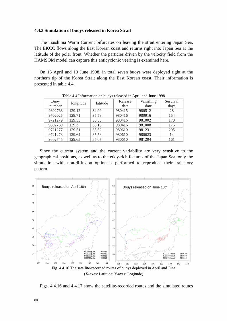
4.4.3 Simulation of buoys released in Korea Strait

The Tsushima Warm Current bifurcates on leaving the strait entering Japan Sea. The EKCC flows along the East Korean coast and returns right into Japan Sea at the latitude of the polar front. Whether the particles driven by the velocity field from the HAMSOM model can capture this anticyclonic veering is examined here.

On 16 April and 10 June 1998, in total seven buoys were deployed right at the

northern tip of the Korea Strait along the East Korean coast. Their information is presented in table 4.4.

Table 4.4 Information on buoys released in April and June 1998 Buoy

number longitude latitude Release

date Vanishing

date Survival

days 9802768 129.12 34.99 980415 980512 28 9702025 129.71 35.58 980416 980916 154 9721279 129.55 35.55 980416 981002 170 9802769 129.3 35.15 980416 981008 176 9721277 129.51 35.52 980610 981231 205 9721278 129.64 35.58 980610 980623 14 9802745 129.65 35.07 980610 981204 161

Since the current system and the current variability are very sensitive to the

geographical positions, as well as to the eddy-rich features of the Japan Sea, only the simulation with non-diffusion option is performed to reproduce their trajectory pattern.

128 130 132 134 136 138 140 142 144

34

36

38

40

42

44

46

48

50 Bouys released on April 16th

9802768p.dat 9804159702025p.dat 9804169721279p.dat 9804169802769p.dat 980416

128 130 132 134 136 138 140 142 144

34

36

38

40

42

44

46

48

50

9721277p.dat 9806109721278p.dat 9806109802745p.dat 980610

Bouys released on June 10th

Fig. 4.4.16 The satellite-recorded routes of buoys deployed in April and June (X-axes: Latitude; Y-axes: Logitude)

Figs. 4.4.16 and 4.4.17 show the satellite-recorded routes and the simulated routes

80

of all seven buoys, respectively. Here, the comparison indicates again that the results of the tracer model are in good agreement with the observations. From this point of view it is fair to say that the HAMSOM model also produces a reasonable velocity field in the southwestern Japan Sea.

Fig. 4.4.17 Simulated routes of all seven buoys in 1998 4.5 Summary

The WOCE/SVP drifters reveal some features of the current field in North East

Asian Regional seas. These features are summarized and plotted in Fig. 4.5.1 for schematic structure.

As discussed in the previous sections, the zonal band east of Taiwan Island is an

eddy-rich zone. The anticyclonic or cyclonic eddies impinge on Taiwan Island every 3 to 4 months. As a result, the area southeast of Taiwan Island is always occupied by eddies. The cyclonic eddies and the anticyclonic eddies may affect the position of the Kuroshio main stream (see <1> in Fig. 4.5.1) east of Taiwan Island by moving it eastward or westward. According to the SVP data, east of Taiwan Island there exists locally an anticyclonic eddy almost all of the time. Just before entering the East China Sea, a branch of the Kuroshio (<2>) flows to the east of the Ryukyu archipelago (<3>) and rejoins the main Kuroshio stream east of Tokara Strait.

After entering East Taiwan Strait, the Kuroshio splits again. The largest part (<4>)

runs northeastward along the 200m depth contour. The rest branching current moves

81

northwestward onto the shelf (<5>). In March and October, cyclonic eddies are always observed from the drifters at the northern coast of Taiwan Island, southwest of the branching current (<6>). Most of the branching current will run northward, rejoin the Kuroshio (<7>) or as part of an anticyclonic motion (<8>) over the central East China Shelf.

According to the buoy data, sometimes the transport in the Taiwan Strait can be

southward. Southwest of Tokara Strait, the Kuroshio turns abruptly from northeast to southeast

(<9>). Here the Kuroshio splits again. The northward branching current (<10>) is thought to be the source of the Tsushima Warm Current and the Huanghai Warm Current. Most of this branching water runs towards the Tsushima Strait (<11>) with part of it flowing eastward to Japan coast, then swirling clockwise back to the Kuroshio main stream in Tokara Strait (<12>). The rest of this branching water moves further northwestward to the western coast of Cheju Island (<13>). North of Cheju Island this flow turns to the right forming the Cheju Warm Current (<14>) which finally heads towards Korea Strait and then follows the East Korean coast northward (<15>).

The outer shelf counter current (<16>) is confirmed by Buoy 9423022 which was

released on 5 October 1994 (Fig. 4.3.13). The Kuroshio countercurrent (<17>) can be seen from the red color buoy trajectory in Fig. 4.3.9a and Buoy 9523909 in Fig. 4.3.4.

Fig. 4.5.1 Schematic current pattern Note: The East Ryukyu Current mentioned in this chapter refers to the surface flow east of the

Ryukyu archipelago.

82

The water exchange across the Ryukyu archipelago is also seen from the SVP data. Pacific water normally intrudes into East China Shelf through the southern Ryukyu archipelago channels and leaves off through the northern channel of Ryukyu archipelago.

Intermittent eddy fields are frequently found east of the Ryukyu archipelago,

southeast of Kyushu and east of the Izu Ridge as indicated in Fig. 4.5.1. A tracer model is developed to reproduce the trajectory fields that revealed by the

satellite buoys. Basing on the velocity and diffusion fields generated by the HAMSOM model, the tracer model qualitatively reproduce the trajectories of the satellite buoys.

The simulated results of arbitrarily selected buoy in three crucial research areas

show that the simulated distributions of the tracer trajectories are generally in good agreement with the satellite traced buoy trajectories. The Kuroshio bifurcation northeast of Taiwan Island and southwest of Kyushu are also found in the tracer model.

83

84

Chapter 5 Discussion of the Kuroshio system in the East China Sea

Observations of the hydrography and water movements in the East China Sea in areas where the bottom topography interferes with the Kuroshio indicate a vigorous exchange between the Kuroshio and the continental shelf water mass that is relatively cool and fresh. South of about 28oN, the Kuroshio runs into the continental shelf and is uplifted. The resulting onshore intrusion of the Kuroshio is compensated by an offshore flow in the surface layer of continental shelf water which is a part of the horizontal circulation created in part by the intrusion itself. North of about 28oN, the blocking of the Kyushu coastal topography forces a turn of the Kuroshio to the east and a separation of part of the Kuroshio flow on its left-hand side. The separation gives rise to the Tsushima Current. Thus, the surface layer flow along the East China Sea continental margin along which the Kuroshio flows is marked by a convergence in the southern stretches and a divergence in the north.

120E 125E 130E 135E 140E

25N

30N

35N

40N

45N

50N

TwStrait-W

Korea TsushimaCheju

JapanWujiu

Yanmei

ChongshengGongguYunaguo

TwStrait-E

Soya-NSoya-S

Tsugaru-NTsugaru-S

Selected grid points for monthly mean stream functionas well as the locations of five cruise sections

PN line

G line

I line

ME line

TK line

Fig. 5.1 Grid points and section lines used to calculate the channel transport

In the numeric model the current pattern may be determined by many factors. The important factors among these are tides, local wind fields, spatial density variations, sea level heights along open boundaries and the effect of topography. The seasonal and annual variability of the Kuroshio transport and the Kuroshio meander is connected to the global climate changes, which are dominated by the solar variability

85

with an annual cycle and of time scales ranging from a decade to a century. As part of the global atmospheric circulation, the Asian monsoon may exert strong effects on the Kuroshio, whereas the Kuroshio variations have a strong impact on the current system of the East China Sea. In this chapter the Kuroshio system and its time dependent variations will be examined. 5.1 Model generated climatology of the stream function 5.1.1 General pattern of the stream function field

Fig. 5.2a Distribution of the streamfunction based on a 6-year numeric integration of a diagnostic study in units Sv (Hsueh et al. 1997)

Fig. 5.2b Distribution of the streamfunction as climatological mean in October based on a 12-year fully prognostic run in units Sv (1990-2001)

The climatological mean and monthly mean model transport in terms of stream

86

function taken over the model domain are calculated based on the 44-year model output. To compare these results with those of former research, a 12-year climatological mean stream function in October of the hindcast run and that of a 6-year diagnostic integration of a diagnostic model research (Hsueh et al. 1997) are presented in Fig. 5.2. Hsueh et al. (1997) studied this area in a diagnostic way, forcing the model with monthly heatflux and getting a final steady state of the Bryan-Cox model after 6-year integration. This is a good reference of a climatological mean, since their integration was diagnostically repeated, until the basin-averaged kinetic energy of the whole model domain reached a constant state.

Obviously the general streamfunction patterns of both panels in Figs. 5.2 are in

good agreement with each other. A strong east Ryukyu current, up to 20 Sv is seen in both figures. East Ryukyu current strength has been reported as 15.6 Sv to 20 Sv east of the Yanmei Island (Yuan et al. 1998; Zhu et al. 2003; Ichikawa et al. 2004), but a climatological transport up to 20 Sv has not been confirmed until now. Figs. 5.2 suggest that most of the transport of the east Ryukyu current originates in the Pacific instead of being fed by the Kuroshio origins. Zhu et al. (2003) suggested that 15 Sv comes from the inner Pacific and 6 Sv from the area east of the Taiwan Island. Southeast of Chongsheng the average transport is about 6.1 Sv northward. Due to the active mesoscale eddies the temporal variability of the average transport is very high; it sometimes reaches 20.8 Sv.

One difference between Figs. 5.2a and 5.2b is the bifurcation of the Kuroshio

southeast of the Taiwan Island shown in Fig. 5.2b. There are three branches, one branch entering the East China Sea through east Taiwan Strait, the middle branch turning right and flowing northeastward, then entering the East China Sea across Ryukyu archipelago. The third branch flows northeastward as East Ryukyu Current and joins the Kuroshio out of the Tokara Strait.

The climatological features of the transport field based on the 44-year hindcast

model run can be examined. Figs. 5.3a and 5.3b show the climatological mean stream function fields in winter (February) and summer (August) time. The patterns of the climatological means reveal the important features of the studied area, which are shown in Figs. 5.2a and 5.2b. Water exchange across Ryukyu archipelago

In both Figs. 5.3a and 5.3b the stream function contours cross the Ryukyu archipelago, this phenomenon is evident both in winter and summer. The water mass normally enters the East China Sea through the channel between the islands Gonggu and Chongsheng and leaves it between islands Yanmei and Chongsheng. The Kuroshio bifurcation

87

The bifurcation in the East China Sea occurs mainly in two areas: at the northeast coast of the Taiwan Island, and southwest of Kyushu before the Kuroshio veers southeastward into the Tokara Strait. This can be seen in the both cases of Figs. 5.3a and 5.3b. Another bifurcation takes place after the Tsushima Current has entered the Tsushima Strait. It is separated into at least two branches in the Japan Sea: one along the North Japan coast and the other along the East Korean coast. An eddy is formed near the southern East Korean coast, its strength varies seasonally.

Fig. 5.3a Climatological monthly mean streamfunction in winter (February, units: Sv) 1958-2001

Fig. 5.3b Climatological monthly mean streamfunction in summer (August, units: Sv) 1958-2001 Origin of the Tsushima Current

88

Interestingly, the model climatology reveals the existence of the so-called Taiwan-Tsushima-Tsugaru current system (TTT-system) in summer time from April to September. Fig. 5.3a shows that in winter the water from the Kuroshio almost covers the whole Tsushima Strait, while in summer (Fig. 5.3b) the Taiwan Warm Current contributes much to the Tsushima Current. The climatological field suggests that the Tsushima Current comes mainly from the Kuroshio in winter, but is composed mainly of both Taiwan Warm Current water and the Kuroshio water in summertime.

The TTT-system has already been studied in several earlier works (Isobe 1999a;

Lin et al. 2002; Fang et al. 1991). Based on the results of a simple diagnostic numerical model, Isobe (1999a) argued that from winter through spring to summer there exists a Taiwan-Tsushima warm current. Lin et al. (2002) studied 142 fixed buoys and 58 satellite traced buoys and found that in the warm half of the year, the Taiwan Warm Current contributes to the Tsushima Warm Current, but in the cold half of the year not. Both their results and the results of this work show that from the climatological field the TTT-system exists from April to September. Fang et al. (1991) made the same conclusion after they had put forward the concept of the TTT-system.

Since Changjiang discharge is small, its role in the TTT-system can not be

explicitly seen in the climatological field. The outer shelf counter current and the east Kuroshio counter current

The outer shelf counter current is not illustrated here due to its small transport. The east Kuroshio counter current can be inferred from the climatological stream function field with seasonally varying strength. It flows southward and forms an anticyclonic closed curve northwest of the Chongsheng Island. The strong anticyclonic eddy northeast of the Tokara Strait

Throughout the whole year a strong eddy exists northeast of the Tokara Strait. Shu (1993) studied the transport across the section normal to the Kuroshio and across the center of this eddy (ASUKA line), he suggested that the volume transport may be as large as 90.6 Sv. Removing the eddy effect, the net Kuroshio transport amounts to approximately 44.4 Sv in this region. Only 18.5 Sv consists of the Kuroshio water from the East China Sea to the Tokara Strait. The remainder of the transport is made up of the northward Pacific water, east of Ryukyu archipelago (Shu 1993). Compared to the model climatological field, a net total Kuroshio transport of about 44.4 Sv across the ASUKA line is reasonable. This implies that the northward Pacific water contributes 25.9 Sv to the whole Kuroshio transport south of Japan, according to Shu’s calculation.

89

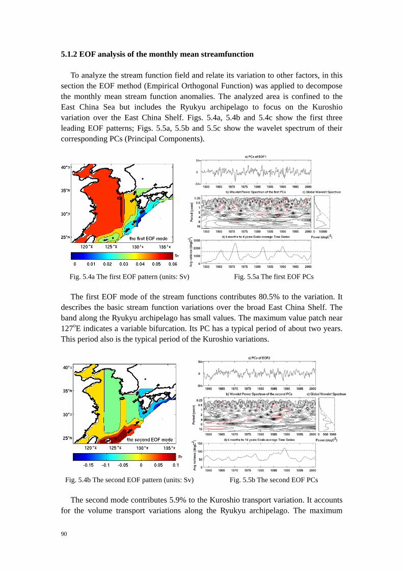
5.1.2 EOF analysis of the monthly mean streamfunction

To analyze the stream function field and relate its variation to other factors, in this section the EOF method (Empirical Orthogonal Function) was applied to decompose the monthly mean stream function anomalies. The analyzed area is confined to the East China Sea but includes the Ryukyu archipelago to focus on the Kuroshio variation over the East China Shelf. Figs. 5.4a, 5.4b and 5.4c show the first three leading EOF patterns; Figs. 5.5a, 5.5b and 5.5c show the wavelet spectrum of their corresponding PCs (Principal Components).

Fig. 5.4a The first EOF pattern (units: Sv) Fig. 5.5a The first EOF PCs

The first EOF mode of the stream functions contributes 80.5% to the variation. It describes the basic stream function variations over the broad East China Shelf. The band along the Ryukyu archipelago has small values. The maximum value patch near 127oE indicates a variable bifurcation. Its PC has a typical period of about two years. This period also is the typical period of the Kuroshio variations.

Fig. 5.4b The second EOF pattern (units: Sv) Fig. 5.5b The second EOF PCs

The second mode contributes 5.9% to the Kuroshio transport variation. It accounts for the volume transport variations along the Ryukyu archipelago. The maximum

90

values cover the southern part of the Ryukyu archipelago. Its PC has typical periods of about 3 years and 5 to 7 years. The latter also is the period of the ENSO phenomenon.

Fig. 5.4c The third EOF pattern (units: Sv) Fig. 5.5c The third EOF PCs

The third mode contributes 2.9% to the whole variation. It accounts for the volume

transport variations across the channels of Ryukyu archipelago. The maximum values are found east of the Ryukyu archipelago. Its PC has typical periods of about 4 years and 5 to 7 years. Again the latter is the period of the ENSO phenomenon.

It should be emphasized here that for all three PCs, a period of 15 to 16 years is

detected. This corresponds to a period of the decadal variability of the long-term Kuroshio transport.

91

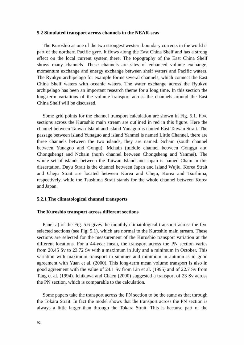
5.2 Simulated transport across channels in the NEAR-seas

The Kuroshio as one of the two strongest western boundary currents in the world is part of the northern Pacific gyre. It flows along the East China Shelf and has a strong effect on the local current system there. The topography of the East China Shelf shows many channels. These channels are sites of enhanced volume exchange, momentum exchange and energy exchange between shelf waters and Pacific waters. The Ryukyu archipelago for example forms several channels, which connect the East China Shelf waters with oceanic waters. The water exchange across the Ryukyu archipelago has been an important research theme for a long time. In this section the long-term variations of the volume transport across the channels around the East China Shelf will be discussed.

Some grid points for the channel transport calculation are shown in Fig. 5.1. Five

sections across the Kuroshio main stream are outlined in red in this figure. Here the channel between Taiwan Island and island Yunaguo is named East Taiwan Strait. The passage between island Yunaguo and island Yanmei is named Little Channel, there are three channels between the two islands, they are named: Schain (south channel between Yunaguo and Gongu), Mchain (middle channel between Gonggu and Chongsheng) and Nchain (north channel between Chongsheng and Yanmei). The whole set of islands between the Taiwan Island and Japan is named Chain in this dissertation. Dayu Strait is the channel between Japan and island Wujiu. Korea Strait and Cheju Strait are located between Korea and Cheju, Korea and Tsushima, respectively, while the Tsushima Strait stands for the whole channel between Korea and Japan. 5.2.1 The climatological channel transports The Kuroshio transport across different sections

Panel a) of the Fig. 5.6 gives the monthly climatological transport across the five selected sections (see Fig. 5.1), which are normal to the Kuroshio main stream. These sections are selected for the measurement of the Kuroshio transport variation at the different locations. For a 44-year mean, the transport across the PN section varies from 20.45 Sv to 23.72 Sv with a maximum in July and a minimum in October. This variation with maximum transport in summer and minimum in autumn is in good agreement with Yuan et al. (2000). This long-term mean volume transport is also in good agreement with the value of 24.1 Sv from Lin et al. (1995) and of 22.7 Sv from Tang et al. (1994). Ichikawa and Chaen (2000) suggested a transport of 23 Sv across the PN section, which is comparable to the calculation.

Some papers take the transport across the PN section to be the same as that through

the Tokara Strait. In fact the model shows that the transport across the PN section is always a little larger than through the Tokara Strait. This is because part of the

92

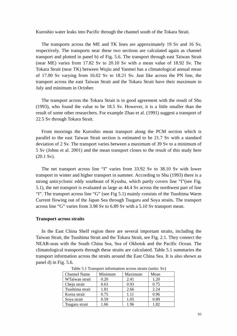
Kuroshio water leaks into Pacific through the channel south of the Tokara Strait. The transports across the ME and TK lines are approximately 19 Sv and 16 Sv,

respectively. The transports near these two sections are calculated again as channel transport and plotted in panel b) of Fig. 5.6. The transport through east Taiwan Strait (near ME) varies from 17.82 Sv to 20.10 Sv with a mean value of 18.92 Sv. The Tokara Strait (near TK) between Wujiu and Yanmei has a climatological annual mean of 17.00 Sv varying from 16.02 Sv to 18.21 Sv. Just like across the PN line, the transport across the east Taiwan Strait and the Tokara Strait have their maximum in July and minimum in October.

The transport across the Tokara Strait is in good agreement with the result of Shu

(1993), who found the value to be 18.5 Sv. However, it is a little smaller than the result of some other researchers. For example Zhao et al. (1991) suggest a transport of 22.5 Sv through Tokara Strait.

From moorings the Kuroshio mean transport along the PCM section which is

parallel to the east Taiwan Strait section is estimated to be 21.7 Sv with a standard deviation of 2 Sv. The transport varies between a maximum of 39 Sv to a minimum of 5 Sv (Johns et al. 2001) and the mean transport closes to the result of this study here (20.1 Sv).

The net transport across line “I” varies from 33.92 Sv to 38.10 Sv with lower

transport in winter and higher transport in summer. According to Shu (1993) there is a strong anticyclonic eddy southeast of Kyushu, which partly covers line “I”(see Fig. 5.1), the net transport is evaluated as large as 44.4 Sv across the northwest part of line “I”. The transport across line “G” (see Fig 5.1) mainly consists of the Tsushima Warm Current flowing out of the Japan Sea through Tsugaru and Soya straits. The transport across line “G” varies from 3.98 Sv to 6.89 Sv with a 5.10 Sv transport mean. Transport across straits

In the East China Shelf region there are several important straits, including the Taiwan Strait, the Tsushima Strait and the Tokara Strait, see Fig. 2.1. They connect the NEAR-seas with the South China Sea, Sea of Okhotsk and the Pacific Ocean. The climatological transports through these straits are calculated. Table 5.1 summaries the transport information across the straits around the East China Sea. It is also shown as panel d) in Fig. 5.6.

Table 5.1 Transport information across straits (units: Sv) Channel Name Minimum Maximum Mean WTaiwan strait 0.20 2.41 1.20 Cheju strait 0.63 0.93 0.75 Tsushima strait 1.81 2.66 2.24 Korea strait 0.75 1.11 0.96 Soya strait 0.59 1.05 0.89 Tsugaru strait 1.66 1.96 1.82

93

Panel a Panel b

Panel c Panel d Fig. 5.6 The climatological mean of the channels transport, details in text

A few works are done on the strait transport around the East China Shelf. Here the

research of Zhao et al. (1991) can be a good reference. They suggested that the transport through the Taiwan Strait is 3.16 Sv in summer and 1.05 in winter. This reasonably compares to the model result (climatological mean from 0.20 to 2.41 Sv). For the Tsushima Strait they suggested a transport of 3.6 Sv, which also is in agreement with the model calculation (climatological mean 2.66 Sv at maximum). Transport across the Ryukyu Archipelago

To examine the water exchange through the Ryukyu archipelago, the long-term channel transports through Ryukyu archipelago are calculated by the model and

94

presented in this section. Table 5.2 summarizes the transport information across the Ryukyu archipelago. The corresponding figure is panel c) in Fig. 5.6. It is shown that the oceanic water enters the East China Shelf mainly through the middle channel with 3.08 Sv. Since the northern channel of the Ryukyu archipelago delivers 2.93 Sv water into Pacific, the long-term mean net transport from oceanic area to shelf area through the Ryukyu archipelago is only 0.48 Sv. The long-term transport of the Dayu Strait is 0.63 Sv.

Table 5.2 Transport information across the Ryukyu archipelago (units: Sv) Channel Name Minimum Maximum Mean Comments Dayu strait 0.43 0.77 0.63 East + Chain -0.64 2.05 0.85 On-shelf + Nchain 2.47 3.38 2.93 Off-shelf + Mchain -3.93 -2.73 -3.08 Off-shelf + Schain 0.14 1.37 0.63 Off-shelf + Little chain -0.23 1.72 0.48 Off-shelf +

To compare the climatological model result with the short-term observations, Fig.

5.7 can be another good reference.

Fig. 5.7 Measured volume transports (a, b, and g), inferred volume transports (c, d, e and f), climatological volume transports (h) and river discharges (i) in Sv for

Oct-Dec, 1999. (W. Teague et al. 2003) 5.2.2 The monthly transport across selected channels and their variations

To study the long-term transport across the channels discussed above, the monthly means of the transports are analyzed using the wavelet method in this section. As we know, the wavelet analysis can extract the information of time series in both frequency and temporal domains.

95

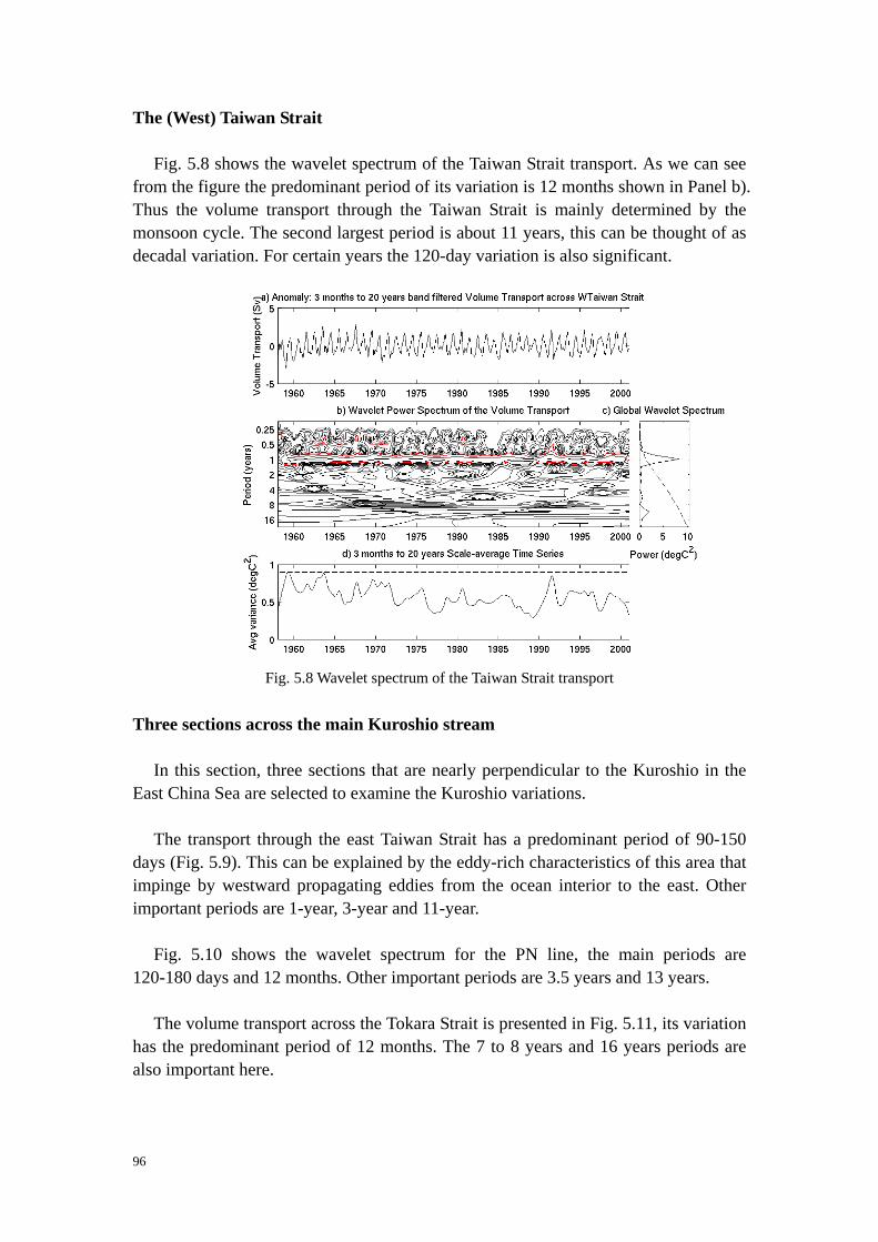
The (West) Taiwan Strait

Fig. 5.8 shows the wavelet spectrum of the Taiwan Strait transport. As we can see from the figure the predominant period of its variation is 12 months shown in Panel b). Thus the volume transport through the Taiwan Strait is mainly determined by the monsoon cycle. The second largest period is about 11 years, this can be thought of as decadal variation. For certain years the 120-day variation is also significant.

Fig. 5.8 Wavelet spectrum of the Taiwan Strait transport Three sections across the main Kuroshio stream

In this section, three sections that are nearly perpendicular to the Kuroshio in the East China Sea are selected to examine the Kuroshio variations.

The transport through the east Taiwan Strait has a predominant period of 90-150

days (Fig. 5.9). This can be explained by the eddy-rich characteristics of this area that impinge by westward propagating eddies from the ocean interior to the east. Other important periods are 1-year, 3-year and 11-year.

Fig. 5.10 shows the wavelet spectrum for the PN line, the main periods are

120-180 days and 12 months. Other important periods are 3.5 years and 13 years. The volume transport across the Tokara Strait is presented in Fig. 5.11, its variation

has the predominant period of 12 months. The 7 to 8 years and 16 years periods are also important here.

96

Fig. 5.9 Wavelet spectrum of the east Taiwan channel transport

Fig. 5.10 Wavelet spectrum of PN line transport

Although all three sections Taiwan Strait, PN line and Tokara Strait cross the Kuroshio, their flow variations have different periods. This can be explained as follows. For the east Taiwan Channel the westward propagating eddies affect the Kuroshio volume transport, the appearance of these eddies have a time scale of 90 to150 days. For the PN line the 12-month period reflects the influence of the Asian monsoon. The two-year time scale variation of Tokara Strait transport is not pronounced here.

97

Fig. 5.11 Wavelet spectrum of Tokara Strait transport The exchange across the middle channel of the Ryukyu archipelago

The wavelet spectrum of the Pacific water across the middle channel of Ryukyu archipelago is shown in Fig. 5.12. A predominant period of 2 years is detected here, the decadal variation is of 13 years.

Fig. 5.12 Wavelet spectrum of middle Ryukyu archipelago channel transport

98

5.3 Analysis of the velocity fields in the East China Shelf

The modification of the upper Kuroshio thermocline occurs primarily along the continental shelf break south of 28oN, where the subsurface water of the Kuroshio is uplifted by the east-west running continental shelf break, generating a surface-layer circulation featuring a flow of cool and less saline shelf water towards the Kuroshio. In the surface layer there is a convergence of continental shelf water towards the Kuroshio south of 28oN.

North of 28oN, the Kuroshio flow diverges mainly due to an upstream effect of the

blockage of the Kyushu coastal topography towards which the Kuroshio is directed. This divergence leads to the formation of the Tsushima Current and supplies the water mass for the Yellow Sea Warm Current. These currents bring tropical heat and salt hundreds of kilometers to the north and are important to the water mass formation in these northern reaches of the marginal seas and, via the Seas of Japan and Okhotsk, to the maintenance of the stratification of the North Pacific Ocean.

In this section the current system in East China Shelf will be examined. Fig. 5.13

shows the surface mean currents of the East China Sea. The long-term mean Kuroshio is also well seen. As comparison Figs. 5.14 present the daily mean surface currents and sea level elevations on 15 February and 15 August of 1994 produced by our hindcast. The daily results are used here to show the current system in the East China Shelf in more details. Obviously, in all four panels of Fig. 5.14 the Kuroshio is well reproduced and illustrated.

Fig. 5.13 Surface mean currents in the East China Sea derived from GEK data from 1953 to 1984 (Qiu et al. 1990)

99

Fig. 5.14a Daily mean velocitiy field on 15 February, 1994

Fig. 5.14b Daily mean velocitiy field on 15 August, 1994

100

Fig. 5.14c Daily sea surface elevation field on 15 February, 1994 (Units: m)

Fig. 5.14d Daily sea surface elevation field on 15 August, 1994 (Units: m)

Fig. 5.14a describes the typical wintertime circulation pattern of the East China

101

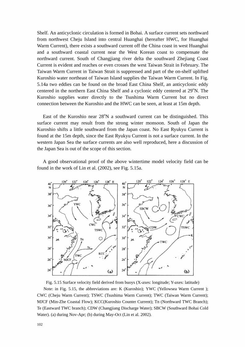
Shelf. An anticyclonic circulation is formed in Bohai. A surface current sets northward from northwest Cheju Island into central Huanghai (hereafter HWC, for Huanghai Warm Current), there exists a southward current off the China coast in west Huanghai and a southward coastal current near the West Korean coast to compensate the northward current. South of Changjiang river delta the southward Zhejiang Coast Current is evident and reaches or even crosses the west Taiwan Strait in February. The Taiwan Warm Current in Taiwan Strait is suppressed and part of the on-shelf uplifted Kuroshio water northeast of Taiwan Island supplies the Taiwan Warm Current. In Fig. 5.14a two eddies can be found on the broad East China Shelf, an anticyclonic eddy centered in the northern East China Shelf and a cyclonic eddy centered at 29oN. The Kuroshio supplies water directly to the Tsushima Warm Current but no direct connection between the Kuroshio and the HWC can be seen, at least at 15m depth.

East of the Kuroshio near 28oN a southward current can be distinguished. This

surface current may result from the strong winter monsoon. South of Japan the Kuroshio shifts a little southward from the Japan coast. No East Ryukyu Current is found at the 15m depth, since the East Ryukyu Current is not a surface current. In the western Japan Sea the surface currents are also well reproduced, here a discussion of the Japan Sea is out of the scope of this section.

A good observational proof of the above wintertime model velocity field can be

found in the work of Lin et al. (2002), see Fig. 5.15a.

Fig. 5.15 Surface velocity field derived from buoys (X-axes: longitude; Y-axes: latitude) Note: in Fig. 5.15, the abbreviations are: K (Kuroshio); YWC (Yellowsea Warm Current );

CWC (Cheju Warm Current); TSWC (Tsushima Warm Current); TWC (Taiwan Warm Current); MJCF (Min-Zhe Coastal Flow); KCC(Kuroshio Counter Current); Tn (Northward TWC Branch); Te (Eastward TWC branch); CDW (Changjiang Discharge Water); SBCW (Southward Bohai Cold Water). (a) during Nov-Apr; (b) during May-Oct (Lin et al. 2002).

102

Fig. 5.14c describes the corresponding daily sea level elevation distribution on 15 February, 1994. The sea levels along the Kuroshio path are strongly intensified within a narrow band. Due to the wintertime monsoon, the sea level height piles up southward along the Zhejiang coast reaching the Taiwan Strait. Over the central Huanghai trough a bulge of the sea surface height appears.

Fig. 5.14b describes the typical summertime circulation pattern of the East China

Shelf. Through the southern Bohai Strait a strong outflow is found to flow out of Bohai. It turns clockwise around the Shandong Peninsula heading to the central Huanghai trough. Over the Huanghai trough there is a broad southward current on 15 August, 1994. South of Shandong Peninsula there is an anticyclonic current and near the southern Korean coast exists a cyclonic current. The Zhejiang Coast Current is now northeastward due to strengthening of the summer monsoon intensified Taiwan Warm Current. But the cyclonic eddy centered on 29oN is still there, since the coastal current near Changjiang river delta was still setting southward.

We can also distinguish the so-called TTT-system in the East China Sea in Fig.

5.14b. The Taiwan Warm Current flows northeastward onto central East China Shelf and partly joins the Kuroshio. At 30oN the remaining Taiwan Warm Current water and part of the Kuroshio water bifurcates from the Kuroshio main stream supplying the source of the Tsushima Warm Current. South of Cheju Island a weak cyclonic eddy can be seen, formed by the southward Huanghai surface water and the northward Taiwan Warm Water.

In summer, east of the Kuroshio near 28oN no southward current at 15m depth

exists any more. This is due to the strong summer monsoon, which suppresses the counter current near the surface layer. A counter current at depth will be discussed later. The Kuroshio flows tightly along the southern Japan coast. No East Ryukyu Current is found at 15m depth either.

Fig. 5.14d describes the corresponding daily sea level elevation distribution on the

same day, 15 August, 1994. The densely crowed sea level contours along the Kuroshio path indicate a good reproduction of the Kuroshio. The dense on the figure sea level contours in the Taiwan Strait implicate the intensified northward Taiwan Strait Warm Current.

Comparing the model result to Fig. 5.15b (Lin et al. 2002), the main difference is

the circulation pattern in the central Huanghai. One plausible explanation is that the summertime circulation in the shallow Huanghai could change its direction frequently due to the variation of surface wind fields. It should be noticed here that the northward coastal current along the southern Korean coast and the southward coastal current near the old Huanghe river delta are confirmed.

To examine the velocity distribution at depth, the velocity fields along some

103

sections that are located in the East China Sea will be examined. For all figures from Fig. 5.16 to Fig. 5.19 the velocity components perpendicular to the section are plotted as the in-out velocity, the velocity component projected in the section plane is plotted as velocity in the section. Every section is laid out from left to right. That means, the positive value indicates the velocity into the paper for the in-out case or the rightward velocity for the velocity projected into the section. 5.3.1 Sections across channels

Fig. 5.16 shows the velocity distribution in section across the channels from Korea Peninsula to the western coast of the Taiwan Strait. On 15 February 1994, the current in the Cheju Strait is mainly eastward, but a westward surface current exists near the northern Cheju Island coast. On 15 August this westward coastal current disappears, the velocity in the Cheju Strait intensifies and flows totally eastward.

Southeast to the Cheju Island a northeastward current exists and near Kyushu a

southward current appears along the Kyushu coast, in February. In August the former becomes larger and the latter becomes deeper. Here the northeastward current should be the Tsushima Current water, which branches off from the Kuroshio.

Volume transport through the Dayu Strait is larger in February while that of the

Tokara Strait strengthens in August. The volume exchange across the Ryukyu archipelago is also larger in August than in February.

At both sides of the Kuroshio main stream axis in the east Taiwan Strait there

exists a weak southward counter current, furthermore the velocity there is larger in August than in February.

The Taiwan Strait also features a seasonal difference as the Cheju Strait. In

February the transport in the western strait reverses its direction to southwest due to the winter monsoon. The maximum southwestward velocities are surface intensified and the northward transport is near the eastern strait bottom. In August, the whole transport in the Taiwan Strait is predominantly northeastward. 5.3.2 Sections surrounding the East China Shelf

Fig. 5.17 shows the sections that envelop the central East China Sea. In February across the northern section the current is mainly northward with a maximum value near the bottom along the 125m contour. Near the surface and at the ends of this section the current is southward. While in August the northward current is confined east of the 100m depth contour and an additional intensified surface northward current is formed. Shallower than 100m in the west the current is southward. Both in February and in August the bottom velocity along the section is westward, i.e. the water uplifts from east to west onto shallow areas.

104

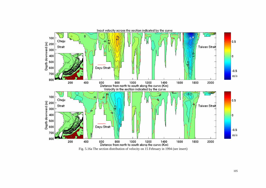
Fig. 5.16a The section distribution of velocity on 15 February in 1994 (see insert)

105

Fig. 5.16b The section distribution of velocity on 15 August in 1994 (see insert)

106

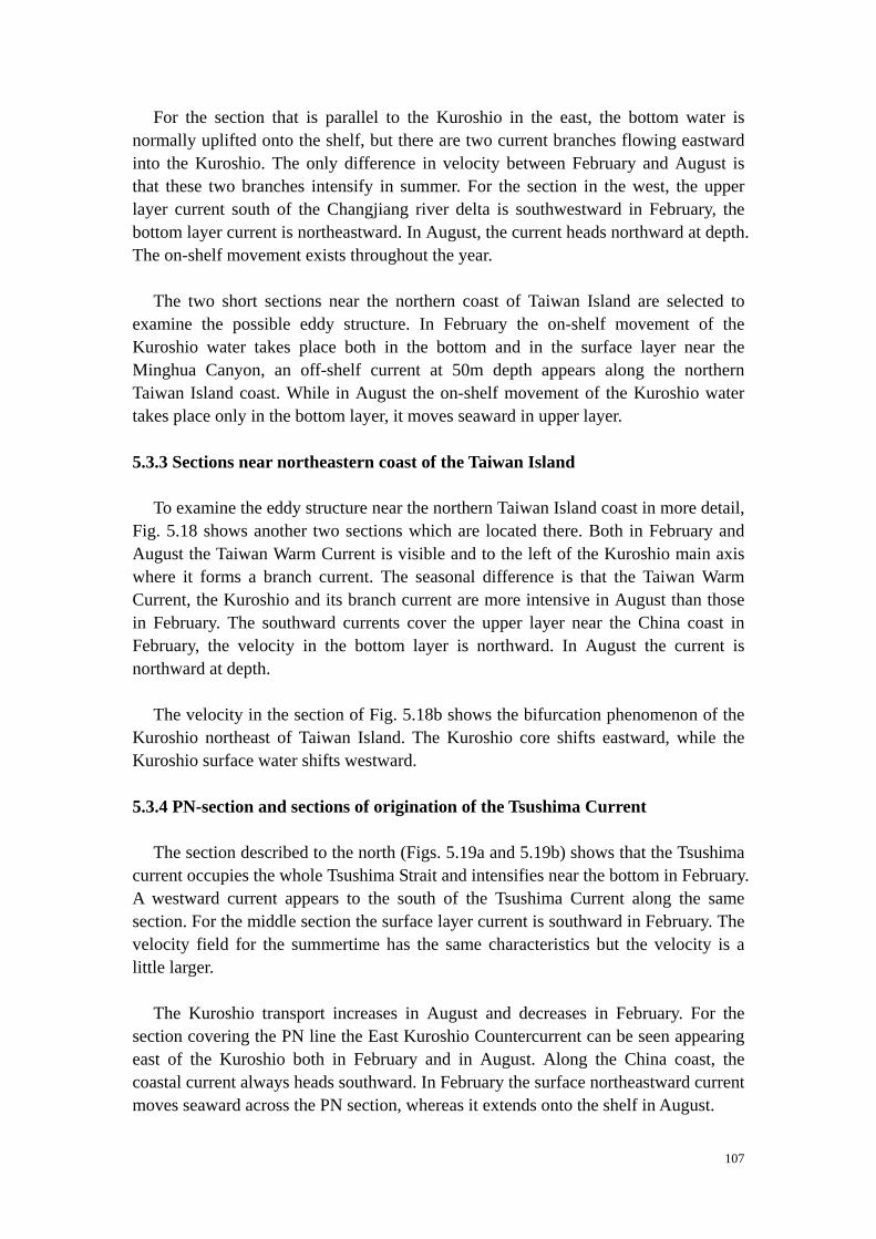
For the section that is parallel to the Kuroshio in the east, the bottom water is normally uplifted onto the shelf, but there are two current branches flowing eastward into the Kuroshio. The only difference in velocity between February and August is that these two branches intensify in summer. For the section in the west, the upper layer current south of the Changjiang river delta is southwestward in February, the bottom layer current is northeastward. In August, the current heads northward at depth. The on-shelf movement exists throughout the year.

The two short sections near the northern coast of Taiwan Island are selected to

examine the possible eddy structure. In February the on-shelf movement of the Kuroshio water takes place both in the bottom and in the surface layer near the Minghua Canyon, an off-shelf current at 50m depth appears along the northern Taiwan Island coast. While in August the on-shelf movement of the Kuroshio water takes place only in the bottom layer, it moves seaward in upper layer. 5.3.3 Sections near northeastern coast of the Taiwan Island

To examine the eddy structure near the northern Taiwan Island coast in more detail, Fig. 5.18 shows another two sections which are located there. Both in February and August the Taiwan Warm Current is visible and to the left of the Kuroshio main axis where it forms a branch current. The seasonal difference is that the Taiwan Warm Current, the Kuroshio and its branch current are more intensive in August than those in February. The southward currents cover the upper layer near the China coast in February, the velocity in the bottom layer is northward. In August the current is northward at depth.

The velocity in the section of Fig. 5.18b shows the bifurcation phenomenon of the

Kuroshio northeast of Taiwan Island. The Kuroshio core shifts eastward, while the Kuroshio surface water shifts westward.

5.3.4 PN-section and sections of origination of the Tsushima Current

The section described to the north (Figs. 5.19a and 5.19b) shows that the Tsushima current occupies the whole Tsushima Strait and intensifies near the bottom in February. A westward current appears to the south of the Tsushima Current along the same section. For the middle section the surface layer current is southward in February. The velocity field for the summertime has the same characteristics but the velocity is a little larger.

The Kuroshio transport increases in August and decreases in February. For the

section covering the PN line the East Kuroshio Countercurrent can be seen appearing east of the Kuroshio both in February and in August. Along the China coast, the coastal current always heads southward. In February the surface northeastward current moves seaward across the PN section, whereas it extends onto the shelf in August.

107

Fig. 5.17a The section distribution of velocity on 15 February in 1994

108

Fig. 5.17b The section distribution of velocity on 15 August in 1994

109

Fig. 5.18a The section distribution of velocity on 15 February in 1994

110

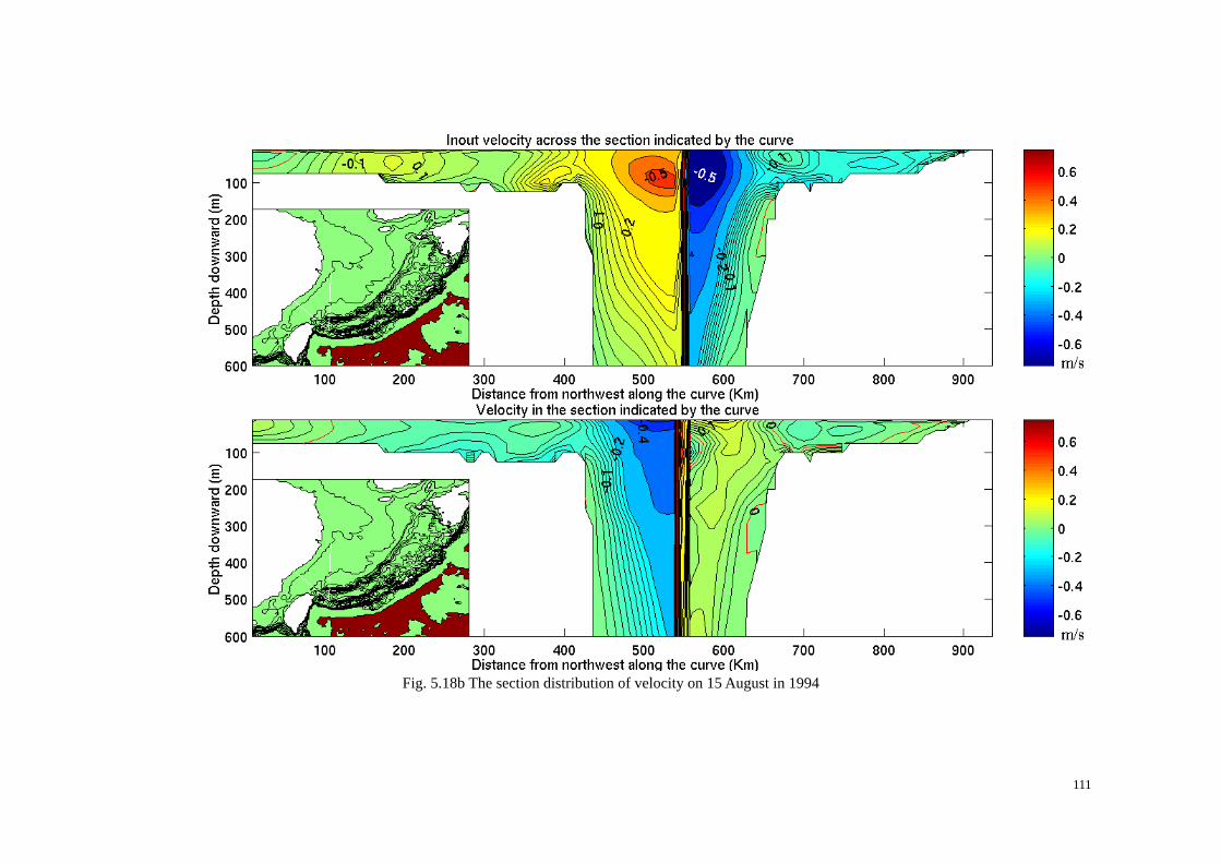
Fig. 5.18b The section distribution of velocity on 15 August in 1994

111

Fig. 5.19a The section distribution of velocity on 15 February in 1994

Fig. 5.19b The section distribution of velocity on 15 August in 1994

113

5.4 Summary

We investigated the transport and velocity field on the East-Chinese Shelf in this chapter. Satisfactory climatological stream function patterns are obtained through the long-term hindcast numerical simulation. The main as well as the detailed characteristics of the flow fields can be distinguished from the climatological fields. For example, the TTT-system on the East-Chinese Shelf, the branching phenomenon of the Tsushima Warm Current from the Kuroshio and the water exchange through the Ryukyu archipelago are confirmed. It is very important to note the existence of the steady and strong northeastward current east of the Ryukyu archipelago. Some earlier modelling work and observations (Zhu et al. 2003; Ichikawa et al. 2000; Yuan et al. 2000) already mentioned this current and now it is confirmed in this numerical investigation, too. An EOF analysis reveals the variation of the Kuroshio. The second EOF mode describes the variability of the Kuroshio path.

The investigation of the volume transports through straits and channels show

reasonable climatological means and also quantitative variabilities. It is shown that the volume transport through the Taiwan Strait is found to be predominated by an annual variation and having a maximum transport value in summer. The climatological volume transport through Taiwan Strait ranges from 1.05 to 3.16 Sv.

Selecting the year 1994 as the sample year, the velocity fields on the East-Chinese

Shelf are also discussed in details. As we already saw in the text, the structure of the Kuroshio and its branch currents are well reproduced by the model. The counter current east of the Kuroshio is also reproduced. The sea level contours along the Kuroshio path are confined to a narrow band, indicating the quasi-geostrophic nature of the Kuroshio.

The extensive discussion of the selected vertical sections on the East-Chinese Shelf

describes vertical structure of the on-shelf intrusion of the Kuroshio across the East China Shelf break, the origination of the Tsushima Warm Current and the eddy field northeast of Taiwan Island. The baroclinic transport in the Taiwan Strait is controlled by the seasonal monsoon. In the western Taiwan Strait, the volume transport reverses its direction seasonally.

The Pacific water intrudes onto the East-Chinese Shelf through the middle channel

of the Ryukyu archipelago, the shelf water leaking into Pacific normally crosses the northern Ryukyu archipelago channel.

In winter, the bottom-intensified northward current covers a large portion of the

zonal section near Cheju Island. In summer, west of the Cheju Island the current reverses its direction to southward flow and east of Cheju Island the northward current strengthens in magnitude and is intensified in the upper layer.

114

Chapter 6 Discussion of the temperature and salinity fields 6.1 Introduction: Climate signals in the Pacific

As part of a larger phenomenon characterized by the Inter Tropical Convergence Zone (ITCZ), the monsoon is a term originally referring to the seasonally shifting winds in the Indian Ocean and surrounding regions. Seasonal monsoon change is characterized by a variety of physical mechanisms, which produce strong seasonal winds, a wet summer and a dry winter. The Asian monsoon affects the Indian subcontinent and southeastern Asia.

The El Niño/Southern Oscillation (ENSO) is the largest known global climate

variability signal on inter-annual time-scales. El Niño was originally a regional name for the annual warming of the Pacific Ocean off the coast of Ecuador and Peru around Christmas time. The appearance of extraordinary warm water over the equatorial central and eastern Pacific is associated with anomalous weather fluctuations elsewhere in the tropics and the extra-tropics, due in part to the influence of SST on the large-scale atmospheric circulation.

The Southern Oscillation is a shift in the relative sea surface pressure values

between large areas of the eastern and western tropical southern Pacific. The ENSO system is a semi-periodic oscillator whose major parameters include the sea surface temperature and pressure, the surface wind and the upper (warm water) layer thickness (ULT). The ENSO associated sea surface temperature changes are Pacific-wide, possibly global in extent, and they are the most important parameter for ENSO monitoring. The wind fields are also important, since it is a principal link between ENSO-related changes in the atmospheric circulation and those of the ocean circulation. The Southern Oscillation index (SOI) describes the phase and amplitude of the Southern Oscillation calculated as the pressure difference (Tahiti minus Darwin). The El Niño events show large negative SOI deviations.

Fig. 6.1a Running average of the Niño 3.4 index from January 1958 to December 2001

Fig. 6.1a shows the Niño 3.47 index from 1958 to 2001 that varies the same as the SOI (Data: Kaplan Sea Surface Temperature. Base period for climatology:

7 Niño 3.4 is defined as the area between 5oN-5oS and 120oW-170oW

115

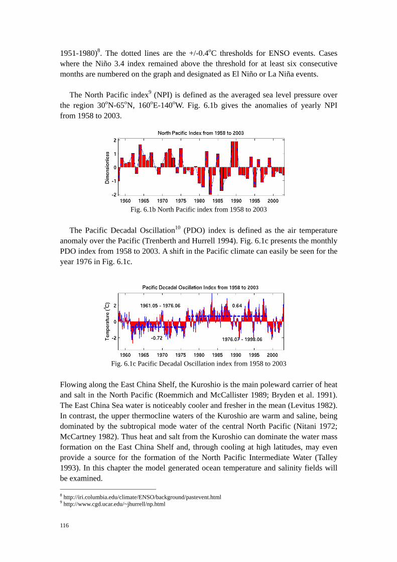
1951-1980)8. The dotted lines are the +/-0.4oC thresholds for ENSO events. Cases where the Niño 3.4 index remained above the threshold for at least six consecutive months are numbered on the graph and designated as El Niño or La Niña events.

The North Pacific index9 (NPI) is defined as the averaged sea level pressure over the region 30oN-65oN, 160oE-140oW. Fig. 6.1b gives the anomalies of yearly NPI from 1958 to 2003.

Fig. 6.1b North Pacific index from 1958 to 2003

The Pacific Decadal Oscillation10 (PDO) index is defined as the air temperature anomaly over the Pacific (Trenberth and Hurrell 1994). Fig. 6.1c presents the monthly PDO index from 1958 to 2003. A shift in the Pacific climate can easily be seen for the year 1976 in Fig. 6.1c.

Fig. 6.1c Pacific Decadal Oscillation index from 1958 to 2003 Flowing along the East China Shelf, the Kuroshio is the main poleward carrier of heat and salt in the North Pacific (Roemmich and McCallister 1989; Bryden et al. 1991). The East China Sea water is noticeably cooler and fresher in the mean (Levitus 1982). In contrast, the upper thermocline waters of the Kuroshio are warm and saline, being dominated by the subtropical mode water of the central North Pacific (Nitani 1972; McCartney 1982). Thus heat and salt from the Kuroshio can dominate the water mass formation on the East China Shelf and, through cooling at high latitudes, may even provide a source for the formation of the North Pacific Intermediate Water (Talley 1993). In this chapter the model generated ocean temperature and salinity fields will be examined. 8 http://iri.columbia.edu/climate/ENSO/background/pastevent.html 9 http://www.cgd.ucar.edu/~jhurrell/np.html

116

6.2 Model generated sea surface climatological fields

The model simulated climate is defined by the means from February, May, August and November in the model period 1958 to 2001 representing winter, spring, summer and autumn, respectively.

In February the warm and saline Kuroshio water is found on the East China Shelf

(Fig. 6.2a, 6.3a). The contours of temperature and salinity bend northwestward from southwest of the Cheju Island into the southern Huanghai and from the northern Huanghai to the northern Bohai Strait. Northeast of the Changjiang river delta these contours bend towards the Kuroshio. In the western Huanghai and eastern Huanghai there exist two warm cores. The temperature along the Bohai and Huanghai coasts is quite low in winter. The salinity around the Huanghe and Changjiang river deltas is quite low due to the fresh discharges.

In May the temperature contours reverse their general direction and bends

southeastward from Shandong Peninsula to the Kuroshio (Fig. 6.2b). The salinity field alters little from February to May but a core with salinity higher than 31 psu appears in the eastern Huanghai (Fig. 6.3b). In August the 34 psu contour line representing the Kuroshio water spreads wider than in February. Judging from the temperature and salinity fields, the Changjiang discharge extends northward along the China coast, while in February it extends much further southward and not as far northward.

In August most surface layer waters in the research area are warmer than 28oC, the

strip-like 27oC patches are seen over the central Huanghai, northwest of the Cheju Strait and in the Taiwan Strait (Fig. 6.2c). The coastal waters around the Bohai and along the western and eastern coasts of the Huanghai are even warmer than 30oC. The water temperature along the southern Shandong coast is remarkable low. According to the salinity field (Fig. 6.3c), the Huanghe discharge runs eastward, and the Changjiang discharge extends further northward than in May along the China coast. The surface salinity of the eastern Huanghai is higher than that in the western part.

In November (Fig. 6.2d) the surface water in the Bohai and Huanghai gets colder

again, but two warm cores appear in the northern Bohai and south of the Shandong Peninsula. Again the Kuroshio dominates the SST field over the outer East China Shelf. In the salinity field (Fig. 6.3d) the Changjiang discharge is seen to spread southwestward along the China coast. The 33 psu contour line covers the Kuroshio main stream axis and extends wider than in August.

From the above discussion, it can be concluded that in the warm half of the year

the solar heating and the Kuroshio cooperate to dominate the sea surface temperature over East China shelf. In the cold half of the year the Kuroshio is dominating the sea surface temperature on the East China Shelf. 10 http://tao.atmos.washington.edu/pdo/

117

Fig. 6.2a Simulated SST distribution in February in oC (1958-2001) and areas of special interest (see text)

Fig. 6.2b Simulated SST distribution in May in oC (1958-2001) and areas of special interest (see text)

118

Fig. 6.2c Simulated SST distribution in August in oC (1958-2001) and areas of special interest (see text)

Fig. 6.2d Simulated SST distribution in November in oC (1958-2001) and areas of special interest (see text)

119

Fig. 6.3a Simulated SSS distribution in February in psu (1958-2001) and areas of special interest (see text)

Fig. 6.3b Simulated SSS distribution in May in psu (1958-2001) and areas of special interest (see text)

120

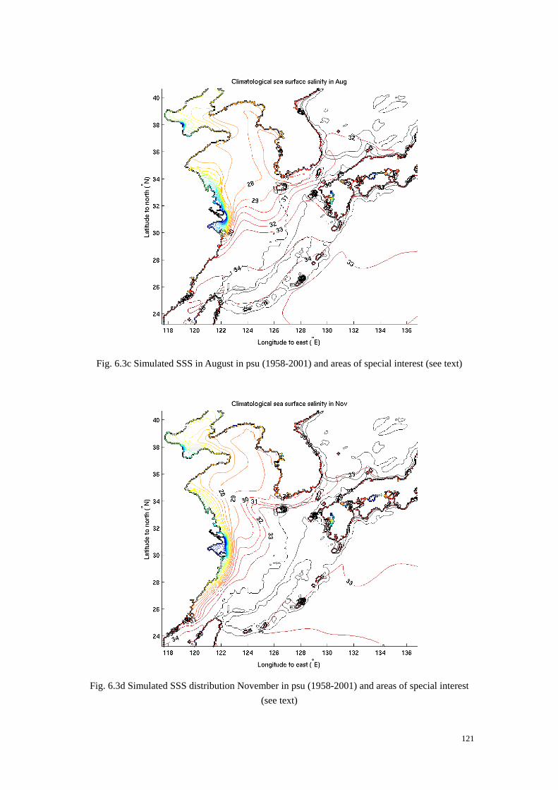
Fig. 6.3c Simulated SSS in August in psu (1958-2001) and areas of special interest (see text)

Fig. 6.3d Simulated SSS distribution November in psu (1958-2001) and areas of special interest (see text)

121

6.3 Long-term variations of surface fields across the PN section

As mentioned in section 6.1, the ENSO associated SST changes are Pacific-wide, in this section the SST field in NEAR-seas will be examined. The SSS field is also to be presented here.

Fig. 6.4a shows the monthly SST anomalies across the PN section from January

1958 to December 2001. Irregular warm and cold events with anomalies higher than 0.5oC across PN section can be distinguished. The big positive anomalies are found in 1960, 1963, 1964, 1966, 1967, 1973, 1975, 1977, 1979, 1983, 1984, 1991, 1992, 1994 and 1998, and the big negative anomalies in 1963, 1965, 1966, 1972, 1976, 1988, 1990, 1997 and 2000.

Fig. 6.4a Time dependent SST anomalies across the PN section in oC (1958-2001)

122

Fig. 6.4b shows the monthly SSS anomalies across the PN section. The salinity variations in the western part of the PN section are strong, while the variations in the eastern part are small. It is interesting to note that the anomalies are generally positive before 1975 and negative after 1975. Large freshening events are found in 1963, 1969, 1972, 1975, 1976, 1993, 1987, 1989, 1991, 1992, 1993, 1998 and 1999. Large salinity anomalies higher than 1.0 psu take place in 1958, 1960, 1965 and 1966.

Fig. 6.4b Time dependent SSS anomalies across the PN section in psu (1958-2001)

To study the possible correlation between the temperature or salinity variability in NEAR-seas and the Pacific climate signals such ENSO several areas are selected in NEAR-seas. The areas are shown with squares in Fig. 6.2a, they are BH (Bohai), NH (Northern Huanghai), SH (Southern Huanghai), NE (Northern East China Sea) and SE (Southern East China Sea). For each of the areas the deviations of the yearly averaged SST are calculated from the mean of the model period 1958 to 2001.

The correlation between SST anomalies in the BH and the NH is 0.77 and between

123

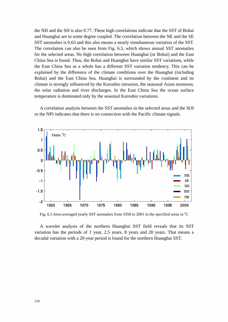
the NH and the SH is also 0.77. These high correlations indicate that the SST of Bohai and Huanghai are to some degree coupled. The correlation between the NE and the SE SST anomalies is 0.63 and this also means a nearly simultaneous variation of the SST. The correlation can also be seen from Fig. 6.5, which shows annual SST anomalies for the selected areas. No high correlation between Huanghai (or Bohai) and the East China Sea is found. Thus, the Bohai and Huanghai have similar SST variations, while the East China Sea as a whole has a different SST variation tendency. This can be explained by the difference of the climate conditions over the Huanghai (including Bohai) and the East China Sea. Huanghai is surrounded by the continent and its climate is strongly influenced by the Kuroshio intrusion, the seasonal Asian monsoon, the solar radiation and river discharges. In the East China Sea the ocean surface temperature is dominated only by the seasonal Kuroshio variations.

A correlation analysis between the SST anomalies in the selected areas and the SOI

or the NPI indicates that there is no connection with the Pacific climate signals.

Fig. 6.5 Area-averaged yearly SST anomalies from 1958 to 2001 in the specified areas in oC

A wavelet analysis of the northern Huanghai SST field reveals that its SST variation has the periods of 1 year, 2.5 years, 8 years and 20 years. That means a decadal variation with a 20-year period is found for the northern Huanghai SST.

124

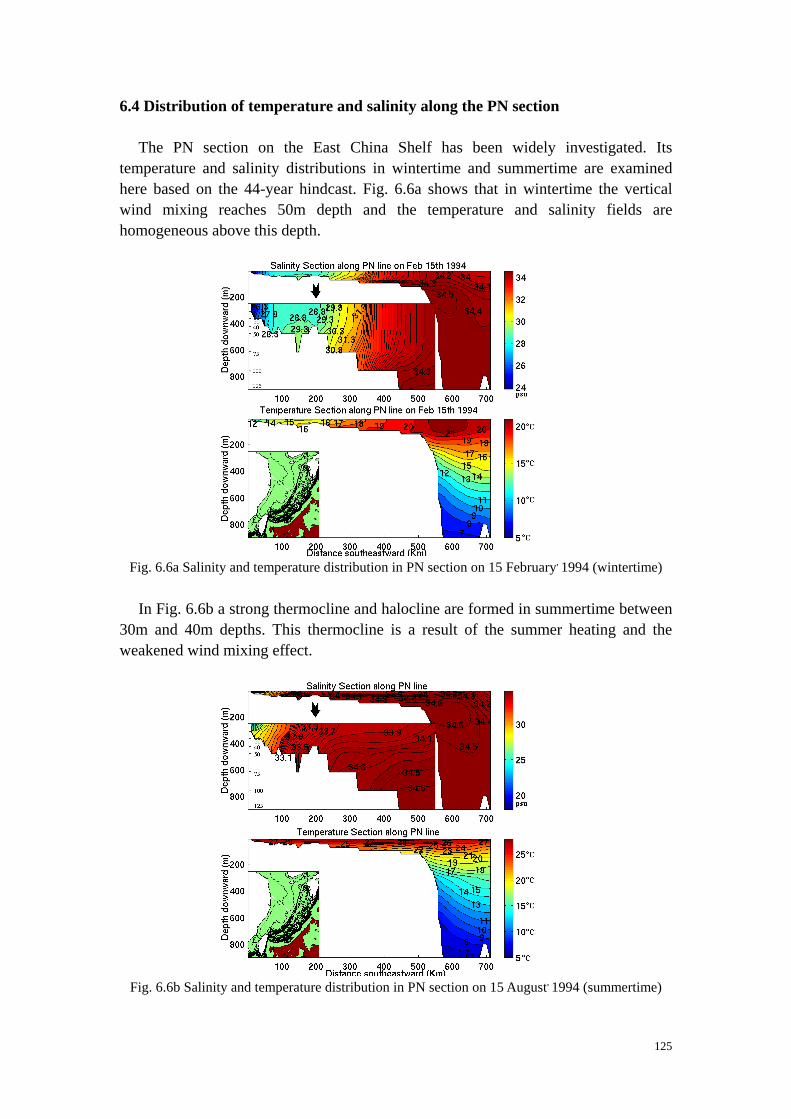
6.4 Distribution of temperature and salinity along the PN section

The PN section on the East China Shelf has been widely investigated. Its temperature and salinity distributions in wintertime and summertime are examined here based on the 44-year hindcast. Fig. 6.6a shows that in wintertime the vertical wind mixing reaches 50m depth and the temperature and salinity fields are homogeneous above this depth.

Fig. 6.6a Salinity and temperature distribution in PN section on 15 February, 1994 (wintertime)

In Fig. 6.6b a strong thermocline and halocline are formed in summertime between 30m and 40m depths. This thermocline is a result of the summer heating and the weakened wind mixing effect.

Fig. 6.6b Salinity and temperature distribution in PN section on 15 August, 1994 (summertime)

125

6.5 Model simulated Huanghai Bottom Cold Water in summertime

Figs. 6.7a shows the temperature and salinity distribution at 50m, 100m and 200m depths in wintertime. At 50m a warm tongue indicated by the 20oC contour lineis seen reaching the southern Kyushu coast and extends eastward through the Tokara Strait. In the Huanghai and northern East China Sea the 16oC contour line extends into central Huanghai. The temperature contours bend into the Bohai. The corresponding salinity field has similar features. That means, in wintertime the warm and salty Kuroshio water extensively intrudes into the inner shelf seas, although the winter monsoon is normally southwestward. Examining the 17oC temperature isoline, it splits around the Cheju Island, indicating the existence of the Huanghai Warm Current and the Tsushima Warm Current.

The temperature and salinity fields at 100m and 200m depths clearly show the

Kuroshio path with steep gradients at both sides of the main stream. Especially at 200m depth a steep temperature gradient exists west of the Kuroshio and the 34.5 salinity isoline implies a narrow-confined Kuroshio path.

Figs. 6.7b shows the temperature and salinity distribution at 50m, 100m and 200m

depths in summertime. The temperature at 50m is significantly different from the winter pattern. The area with a 24oC temperature spreads widely over the East China Shelf accompanied by some patch-like areas of 23oC or 25oC. The 24oC water mass is found west of Kyushu and even in the southern Tsushima Strait and the Tokara Strait. In most areas of the Huanghai the temperature contours of 15oC and 16oC are bending southward. The 18oC temperature isoline is found west of the Cheju Strait. The lowest temperature center is located in the northern Huanghai. The summer salinity pattern is different from the summer temperature pattern and generally similar to the winter salinity pattern. A small closed salinity contour can be seen in the central eastern Huanghai. The 33.4 psu contour splits southwest of Kyushu, indicating the existence of the Huanghai Warm Current and the Tsushima Warm Current. In summer the summer heating, monsoon and precipitation cooperate to affect the local ocean climate on the East China Shelf.

In the temperature pattern at 100m depth, a cold band is seen north of the Taiwan

Island. The closed 20oC contour line implies a cold eddy lying there at 100m depth. According to the analysis in Chapter 5 this should be an anticyclonic eddy created by the on-shelf current in the north and the descending current along the northern Taiwan Island coast in the south. This cold eddy means that in summer there exists upwelling, which convects the deep layer cold Kuroshio water to the surface water in this area. Further northward, there is another small closed 20oC temperature contour which is a result of the weak cyclonic gyre there.

126

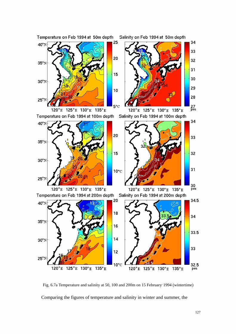
Fig. 6.7a Temperature and salinity at 50, 100 and 200m on 15 February, 1994 (wintertime)

Comparing the figures of temperature and salinity in winter and summer, the

127

Fig. 6.7b Temperature and salinity at 50, 100 and 200m on 15 August, 1994 (summertime) summer heating and winter cooling are as important as the seasonal monsoon in the surface layers. The surface temperature field variation is large, since it is sensible to

128

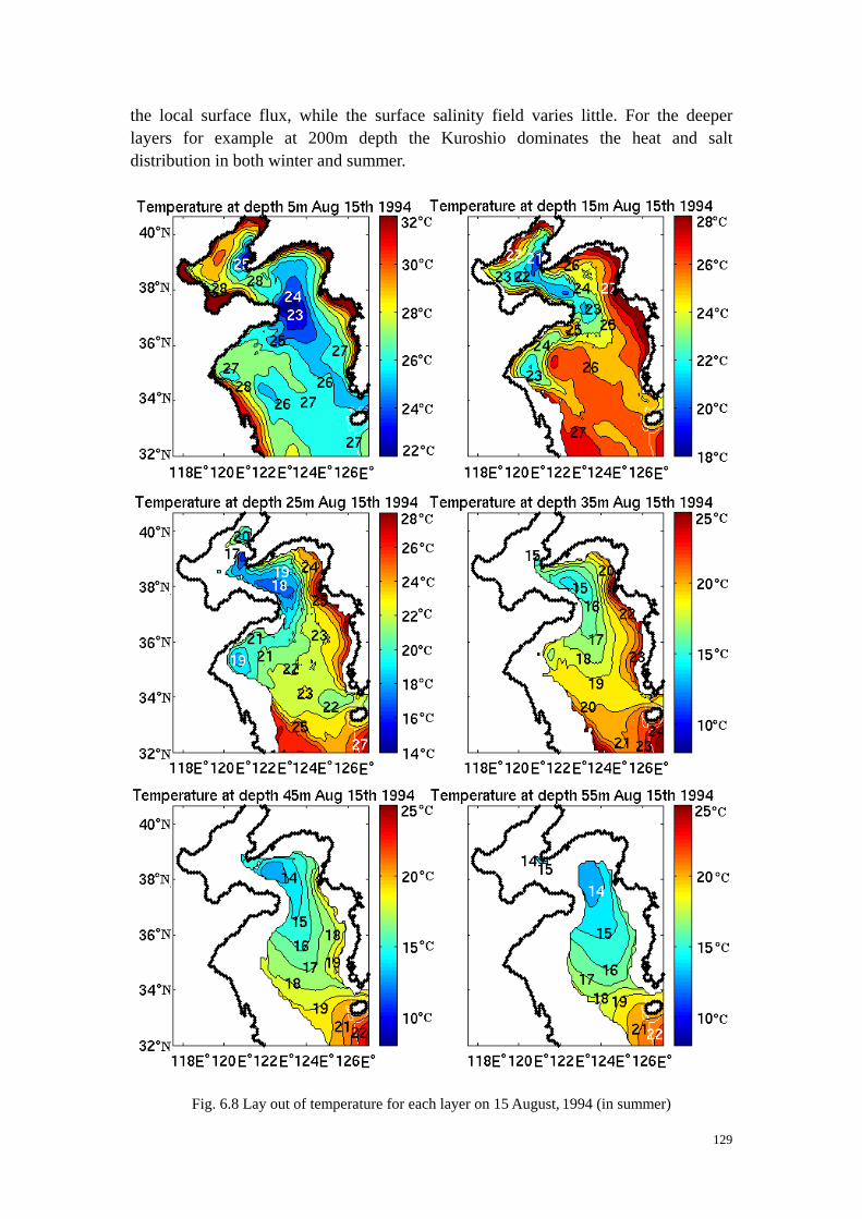
the local surface flux, while the surface salinity field varies little. For the deeper layers for example at 200m depth the Kuroshio dominates the heat and salt distribution in both winter and summer.

Fig. 6.8 Lay out of temperature for each layer on 15 August, 1994 (in summer)

129

In summer the Huanghai Bottom Cold Water (HBCW) which is located from the Bohai Strait to the central Huanghai trough is well conserved. Fig. 6.8 depicts its horizontal temperature distribution for the upper six layers in summer.

In the upper three layers in Fig. 6.8, especially in the layer of 25m depth, three cold

water centers can be seen in the Huanghai basin. One is near the western coast of the Liaodong Peninsula in the Bohai and two in the Huanghai. The largest cold center in northern Huanghai is the HBCW and the smaller one southeast of the Shandong Peninsula results from an anticyclonic eddy there. The temperature patterns of the layers 4 to 6 well describe the features of the HBCW at depth.

The area which is colder than 16oC is increasing from 35m depth down to 55m,

where it covers the whole Huanghai Trough.

Fig. 6.9a Vertical salinity and temperature distribution across Huanghai in winter (15 February, 1994)

Figs. 6.9a and 6.9b show the distributions of temperature and salinity along a

meridional section over the Huanghai Trough in winter and in summer. These figures combined with Fig. 6.8 give a clear illustration of the HBCW distribution.

In Fig. 6.9b a strong thermocline and halocline are seen over the Huanghai Trough between 30m and 40m. It should be noticed that both the temperature and the salinity contours vault near the center of HBCW. In the temperature field, the 24oC contour line outcrops at the surface. This phenomenon results from the upwelling induced by the basin wide cyclonic circulation. In Fig. 6.9a strong vertical wind mixing in winter makes the whole water column homogeneous, no thermocline is formed at that time .

130

Fig. 6.9b Vertical salinity and temperature distribution across Huanghai in summer (15 August, 1994)

Furthermore, it should be noted that the Huanghai bottom water is fresher in winter

than that in summer. 6.6 Summary

In this chapter the model simulated ocean temperature and salinity fields on the East-Chinese Shelf have been investigated. Based on the analysis of the model results it can be concluded that, although the long-term temperature fields are well reproduced by the hindcast simulation, no direct correlation between the long-term model generated SST variation on the East-Chinese Shelf and the global or Pacific climate signal is found. The reason might be due to the strong local seasonal monsoon, the summer (winter) heating (cooling) and the shallowness of the shelf waters. Thus, the impact of these factors on East-Chinese Shelf climate is as important as that of the forcing from the global or Pacific climate system. The Kuroshio dominates the variations of the ocean surface temperature and salinity along the shelf breaks and on the East-Chinese Shelf.

A correlation analysis on the temperature and salinity variations from different

areas shows that the variations of the model SST fields in the Bohai and Huanghai are correlated, but they are not correlated with the variations in the East China Sea.

The long-term ocean temperature and salinity variations along the PN section were

examined. In winter, the shallow shelf waters are well mixed at depth and no

131

thermocline is developed. The mixed layer reaches approximately 50m depth in the oceanic Kuroshio area. In summer, a well-developed thermocline and halocline in the shallow shelf area as well as in the oceanic Kuroshio area are produced. A strong thermocline is developed at 30m to 40m except in the area along the China coast. The existence of the thermocline in summer but not in winter indicates that the local seasonal atmospheric forcing variation plays an important role in the upper ocean layer. The Kuroshio dominates the temperature variation in the remaining deeper parts.

The role of the Kuroshio is much more clearly illustrated by examining the ocean

temperature and salinity fields at the depths of 50m, 100m and 200m. The Kuroshio water dominates the ocean temperature and salinity in each of these depths both in winter and summer. The temperature and salinity fronts west of the Kuroshio on the East-Chinese Shelf are clearly shown in each depth. The temperature distribution at 50m in winter shows the branching of the Tsushima Current and the Huanghai Warm Current around the Cheju Island. A cold eddy at the northern Taiwan Island coast is detected at 100m depth and indicates the existence of upwelling.

At last the Huanghai Bottom Cold Water (HBCW) in summer was discussed. The

existence of the HBCW in summer is proven and its variation with depth is described. The HBCW is conserved in the central Huanghai basin and the thermocline and halocline are well developed over the HBCW. The thermocline and halocline are destroyed in winter by the strong vertical mixing due to the winter monsoon and the winter cooling. The whole water column is well-mixed from surface to bottom and the temperature and salinity contours are vertically in a chimney-like shape.

132

Chapter 7 Discussion of the Joint Effect of Baroclinicity and Relief

(JEBAR) 7.1 Introduction to JEBAR

The JEBAR-term as an abbreviation stands for the Joint Effect of Baroclinicity and Relief. It emerges from the vorticity equation that is formed from the depth-averaged momentum equations and is defined as the Jacobian of the baroclinic potential energy

χ and inverse ocean depth . Here, the baroclinic potential energy is

defined as

),(/1 yxH

∫ −=⋅≡

0

0Hz

dzzg ρρ

χ (7-1)

where g is the gravitational acceleration, ρ is the in-situ density, 0ρ is the

reference density, is the vertical coordinate and z H is ocean depth. Since its first description by Sarkisyan and Ivanov (1971) and extensive discussion

by Sarkisyan (1977) the JEBAR-term has been studied in numerous publications (Rattray 1982; Huthnance 1984; Csanady 1985; Mertz and Wright 1992; Cane, Kamenkovich and Krupitsky 1998; Pohlmann 1999, 2003). In most publications it is taken as a ‘forcing term’ that drives the depth-integrated transport across isobaths; that means, a barotropic current is induced by JEBAR to satisfy the condition of no divergence of the horizontal transport when the density varies along isobaths. Greatbatch et al. (1991) calculated the circulation in the North Atlantic in a diagnostic way. To interpreted the results from the theoretical point of view, they separated the JEBAR-term into two parts: the bottom pressure torque induced by the interaction of bottom pressure and bottom topography, and the compensation by the density stratification for the effect of variable bottom topography. With the help of the JEBAR terminology, Mertz and Wright (1992) interpreted the vorticity equation of the depth-averaged flow as the depth-integrated transport across geostrophic potential vorticity contours f/H and determined by the JEBAR-term, the curl of the wind stress

H/τr and frictional as well as nonlinear effects (here f is the Coriolis parameter). Using the JEBAR-term as a ‘forcing term’, Myers et al. (1996) developed a diagnostic, finite element, barotropic ocean model to simulate the mean circulation in the North Atlantic. They found that the Gulf Stream separates at the correct latitude off Cape Hatteras with the JEBAR included and the JEBAR-term in three key regions is crucial in determining the Gulf Stream separation point.

133

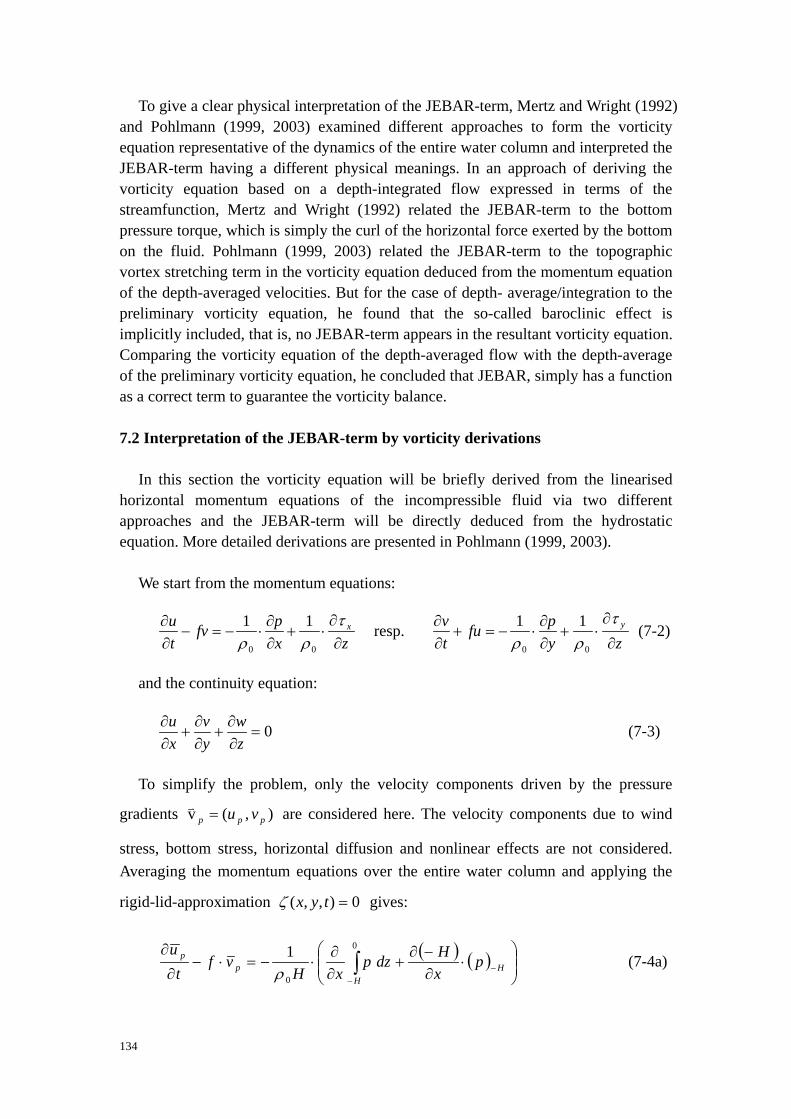
To give a clear physical interpretation of the JEBAR-term, Mertz and Wright (1992) and Pohlmann (1999, 2003) examined different approaches to form the vorticity equation representative of the dynamics of the entire water column and interpreted the JEBAR-term having a different physical meanings. In an approach of deriving the vorticity equation based on a depth-integrated flow expressed in terms of the streamfunction, Mertz and Wright (1992) related the JEBAR-term to the bottom pressure torque, which is simply the curl of the horizontal force exerted by the bottom on the fluid. Pohlmann (1999, 2003) related the JEBAR-term to the topographic vortex stretching term in the vorticity equation deduced from the momentum equation of the depth-averaged velocities. But for the case of depth- average/integration to the preliminary vorticity equation, he found that the so-called baroclinic effect is implicitly included, that is, no JEBAR-term appears in the resultant vorticity equation. Comparing the vorticity equation of the depth-averaged flow with the depth-average of the preliminary vorticity equation, he concluded that JEBAR, simply has a function as a correct term to guarantee the vorticity balance. 7.2 Interpretation of the JEBAR-term by vorticity derivations

In this section the vorticity equation will be briefly derived from the linearised horizontal momentum equations of the incompressible fluid via two different approaches and the JEBAR-term will be directly deduced from the hydrostatic equation. More detailed derivations are presented in Pohlmann (1999, 2003).

We start from the momentum equations:

zxpfv

tu x

∂∂

⋅+∂∂

⋅−=−∂∂ τ

ρρ 00

11 resp. zy

pfutv y

∂

∂⋅+

∂∂

⋅−=+∂∂ τ

ρρ 00

11 (7-2)

and the continuity equation:

0=∂∂

+∂∂

+∂∂

zw

yv

xu (7-3)

To simplify the problem, only the velocity components driven by the pressure

gradients ),(v ppp vu=v are considered here. The velocity components due to wind

stress, bottom stress, horizontal diffusion and nonlinear effects are not considered. Averaging the momentum equations over the entire water column and applying the

rigid-lid-approximation 0),,( =tyxζ gives:

( ) ( ) ⎟⎟⎠

⎞⎜⎜⎝

⎛⋅

∂−∂

+∂∂

⋅−=⋅−∂

∂−

−∫ HH

pp p

xHdzp

xHvf

tu 0

0

1ρ

(7-4a)

134

( ) ( ) ⎟⎟⎠

⎞⎜⎜⎝

⎛⋅

∂−∂

+∂∂

⋅−=⋅+∂

∂−

−∫ HH

pp p

yHdzp

yHuf

tv 0

0

1ρ

(7-4b)

where the depth-averaged velocities are:

∫−

≡01

Hpp dzu

Hu resp. ∫

−

≡01

Hpp dzv

Hv (7-5)

After cross-wise differentiating Eqs. (7-4) and applying the hydrostatic

approximation ρ⋅−=∂∂ g

zp as well as the Boussinesq approximation, and a series of

deductions the vorticity equation finally reads:

( ) ⎟⎠⎞

⎜⎝⎛+∇•⋅+∇•−=

∂∂

HJH

Hff

t hphpp1,vvˆ χξ

rrrr (7-6)

where ),(v ppp vu=r

, the relative vorticity is defined as pξ̂y

ux

v ppp ∂

∂−

∂

∂≡ξ̂ and

the Jacobian operator is expressed as xB

yA

yB

xABAJ

∂∂

⋅∂∂

−∂∂

⋅∂∂

≡),( .

According to Eq. (7-6) the time variation of the relative vorticity of the

depth-averaged pressure driven circulation is influenced by depth-averaged currents perpendicular to planetary vorticity contour lines (right side term 1), topographically induced stretching or squeezing of the water body containing planetary vorticity (right side term 2) and the JEBAR effect (right side term 3).

If we define as the depth-integrated transport induced by

the pressure gradient, it follows:

dzviuH

ppp ∫−

+≡0

)j (Mvvv

⎟⎠⎞

⎜⎝⎛

∂∂

+⎟⎠⎞

⎜⎝⎛

∂∂

=⎟⎠⎞

⎜⎝⎛∇• ∫∫

−− Hf

ydzv

Hf

xdzu

Hf

Hp

Hpp M

00vv (7-7)

−⎟⎟⎠

⎞⎜⎜⎝

⎛

∂∂

+∂∂

= ∫∫−−

1 1 00

yfdzv

Hxfdzu

H Hp

Hp

⎟⎟⎠

⎞⎜⎜⎝

⎛

∂∂

+∂∂

∫∫−− y

HdzvHx

HdzuHH

f

Hp

Hp 1 1

00

( )HHff hphp ∇•⋅−∇•=

rrrrvv

135

Thus, using the relations of Eq. (7-7), the vorticity Eq. (7-6) can be rewritten as:

⎟⎠⎞

⎜⎝⎛=⎟

⎠⎞

⎜⎝⎛∇•+

∂∂

HJ

Hf

t pp1,Mˆ χξ

vv (7-8)

The second term in Eq. (7-8) represents the advection of the geostrophic potential

vorticity . This final equation means that for the circulation driven by pressure

gradient, the depth-integrated transport across geostrophic potential vorticity contours are balanced by the JEBAR-term and the time derivative of the relative vorticity.

Hf /

Another way to derive the vorticity equation starts with a crosswise differentiation

of Eq. (7-2) to get the vorticity equation in its velocity form. Then after depth-averaging this vorticity equation the final vorticity equation reads:

( )H)Hff

t hHpp ∇•⋅+∇•−=∂∂

−

rrrrph v(vξ (7-9)

In this case the JEBAR-term is not evolving, which means that the baroclinicity effect must have been expressed implicitly. The depth-averaged velocity is also replaced by the bottom velocity in the vortex stretching term here.

The difference between Eqs. (7-6) and (7-9) leads to one formulation of JEBAR-term:

( ) ⎟⎠⎞

⎜⎝⎛+∇•⋅=−

∂∂

HJH

Hf

t hppp1,v~)ˆ( χξξ

rr (7-10)

where ))(,)(()~,~(v~ HppHppp vvuuvu −− −−≡=r

is the difference between

depth-averaged velocity and the bottom velocity. For the stationary or quasi-stationary

case, the time dependent term in Eq. (7-10) cancels out ⎟⎟

⎠

⎞

⎜⎜

⎝

⎛≈

∂

∂≈

∂

∂0

ˆ

ttpp ξξ

, which also

means that a pure geostrophic equilibrium is considered. Obviously, in this pure geostrophic case the JEBAR-term is a correction term to the vortex stretching term, in which the velocity used is the depth-averaged velocity instead of the bottom velocity. It is reasonable since for kinematic boundary conditions, it is the bottom velocity that is responsible for the topographically vortex stretching of the water column, instead of the depth-averaged velocity.

The above discussion also holds in the non-stationary case, the only difference is

an additional term, which can also be expressed by the difference between the

136

depth-averaged velocity and the bottom velocity. That is, the difference between

pp ξξ −ˆ can be expressed as (Pohlmann 2003):

⎟⎟⎠

⎞⎜⎜⎝

⎛⋅

∂∂

−⋅∂∂

⋅⎟⎠⎞

⎜⎝⎛−=− pppp u

yHv

xH

H~~1ˆ ξξ (7-11)

With relation (7-11) employed, the formulation of the JEBAR-term now reads:

( ) ⎟⎟⎠

⎞⎜⎜⎝

⎛⎟⎟⎠

⎞⎜⎜⎝

⎛∂∂

⋅−∂∂

⋅⋅⎟⎠⎞

⎜⎝⎛−

∂∂

+∇•⋅−=⎟⎠⎞

⎜⎝⎛

yHu

xHv

HtH

Hf

HJ pphp

~~1v~1,rr

χ (7-12)

According to relation (7-12) the additional term corrects the temporal deviation of

the relative vorticity in Eq. (7-6). To get a deeper physical understanding of

the JEBAR-term, Pohlmann (1999, 2003) also directly derived the JEBAR-term by utilization of the hydrostatic equation.

tp ∂∂ /ξ̂

Using the geostrophic equilibrium from Eqs. (7-2):

gfvxp

−=∂∂

⋅−0

1ρ

resp. gfuyp

=∂∂

⋅−0

1ρ

the final JEBAR-term formula is obtained as follows:

( HHf

HJ hg ∇•⋅−=⎟

⎠⎞

⎜⎝⎛ rr

v~1,χ ), (7-13)

where ))(,)(()~,~(v~ HggHggggg vvuuvu −− −−==r

.

Thus, Eq. (7-13) clearly shows that only the geostrophic part of the difference

between depth-averaged and bottom velocity gv~r

enters the JEBAR-term. According

to relation (7-12) the ageostrophic parts of the difference enter the additional

time-dependent term ⎟⎟⎠

⎞⎜⎜⎝

⎛⎟⎟⎠

⎞⎜⎜⎝

⎛∂∂

⋅−∂∂

⋅⋅⎟⎠⎞

⎜⎝⎛−

∂∂

yHu

xHv

Ht pp~~1 . From the discussion above it

can be concluded that the nature of JEBAR is nothing but a transport-generating correct term. Only in a diagnostic calculation of the circulation with the density specified, it can be regarded as a ‘forcing’ term, if one assumes the depth-averaged vorticity to be responsible for the vortex stretching.

137

7.3 Distribution of JEBAR-term in NEAR-Seas 7.3.1 A simple review of JEBAR research in the NEAR-Seas

Some research work on the role of the JEBAR-term was already done in the NEAR-Seas (Isobe, 1994, 1997, 2000; Guo et al. 2003). It is expected that JEBAR plays an important role in NEAR-seas since the topography is complicated and its density variation is larger than in the adjacent oceanic areas.

Using a diagnostic numeric model with JEBAR calculated from the CTD in-situ

observations, Isobe (1994) studied the seasonal current variation in the Tsushima Strait. He argued that the JEBAR is mainly caused by the bottom cold water intrusion into the strait along the Korean coast in summer and this process locally supplies negative vorticity to force the coastal current intensification. Then Isobe (1997) suggested the existence of the bottom cold water and the sea surface heating in summer as a mechanism to interpret the Tsushima Warm Current bifurcation in the Tsushima Strait. His numerical model indicated that JEBAR and the topographic vortex stretching effect are predominant around the shelf slope in the Tsushima Strait. This vortex divergence effect induced by the shelf slope crossing of the East Korean Warm Current cancels the JEBAR effect.

Using a triply nested ocean model Guo et al. (2003) simulated the Kuroshio and

studied the influence of the horizontal resolution on JEBAR reproduction. They found that models with higher-resolutions can improve the baroclinic as well as the barotropic component of the Kuroshio, reproducing more realistic density and current fields, and correct JEBAR values. With a lower-resolution model configuration, the JEBAR values averaged over the same selected area are incorrect, they even have the opposite sign. But Guo et al. (2003) didn’t give an explanation for such improvement of JEBAR reproduction related to the higher model resolution. They studied the Kuroshio veering phenomenon at (30°N, 128-129°E) southwest of Kyushu and concluded that JEBAR and the geostrophic potential vorticity advection are two major contributions to the vorticity balance in the Kuroshio veering area (28-30°N, 126-128°E).

It is interesting to note that the model described by Guo et al. (2003) with a

resolution of 1/6 degree failed to reproduce “correct” JEBAR values. Meanwhile, it can be found in both Isobe (1997) and Guo et al. (2003) that JEBAR and the geostrophic potential vorticity advection are two major contributions to the vorticity balance in both research areas. However, the vortex stretching part is the predominant one in the geostrophic potential vorticity equation.

7.3.2 JEBAR distribution in the NEAR-Seas

138

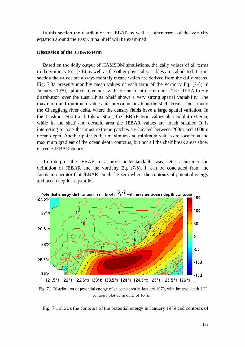
In this section the distribution of JEBAR as well as other terms of the vorticity equation around the East China Shelf will be examined. Discussion of the JEBAR-term

Based on the daily output of HAMSOM simulations, the daily values of all terms in the vorticity Eq. (7-6) as well as the other physical variables are calculated. In this section the values are always monthly means which are derived from the daily means. Fig. 7.3a presents monthly mean values of each term of the vorticity Eq. (7-6) in January 1979, plotted together with ocean depth contours. The JEBAR-term distribution over the East China Shelf shows a very strong spatial variability. The maximum and minimum values are predominant along the shelf breaks and around the Changjiang river delta, where the density fields have a large spatial variation. In the Tsushima Strait and Tokara Strait, the JEBAR-term values also exhibit extrema, while in the shelf and oceanic area the JEBAR values are much smaller. It is interesting to note that most extreme patches are located between 200m and 1000m ocean depth. Another point is that maximum and minimum values are located at the maximum gradient of the ocean depth contours, but not all the shelf break areas show extreme JEBAR values.

To interpret the JEBAR in a more understandable way, let us consider the

definition of JEBAR and the vorticity Eq. (7-8). It can be concluded from the Jacobian operator that JEBAR should be zero where the contours of potential energy and ocean depth are parallel.

Fig. 7.1 Distribution of potential energy of selected area in January 1979, with inverse depth 1/H contours plotted in units of 10-3m-1

Fig. 7.1 shows the contours of the potential energy in January 1979 and contours of

139

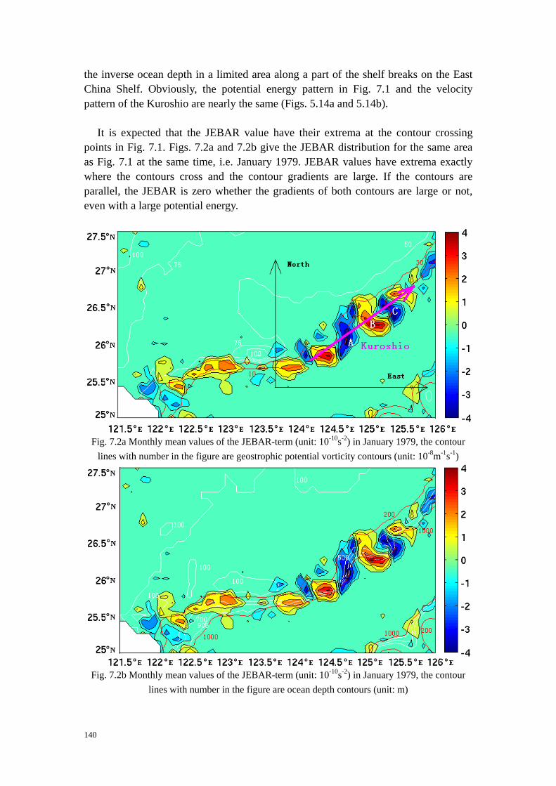
the inverse ocean depth in a limited area along a part of the shelf breaks on the East China Shelf. Obviously, the potential energy pattern in Fig. 7.1 and the velocity pattern of the Kuroshio are nearly the same (Figs. 5.14a and 5.14b).

It is expected that the JEBAR value have their extrema at the contour crossing

points in Fig. 7.1. Figs. 7.2a and 7.2b give the JEBAR distribution for the same area as Fig. 7.1 at the same time, i.e. January 1979. JEBAR values have extrema exactly where the contours cross and the contour gradients are large. If the contours are parallel, the JEBAR is zero whether the gradients of both contours are large or not, even with a large potential energy.

Fig. 7.2a Monthly mean values of the JEBAR-term (unit: 10-10s-2) in January 1979, the contour lines with number in the figure are geostrophic potential vorticity contours (unit: 10-8m-1s-1)

Fig. 7.2b Monthly mean values of the JEBAR-term (unit: 10-10s-2) in January 1979, the contour lines with number in the figure are ocean depth contours (unit: m)

140

If we look at monthly mean field as in the quasi-steady state, Eq. (7-8) will approximately reduce to the relation below:

⎟⎠⎞

⎜⎝⎛≈⎟

⎠⎞

⎜⎝⎛∇•

HJ

Hf

p1,M χ

vv (7-14)

Now that the JEBAR has been directly calculated from the model results, it can be seen as a forcing term in a diagnostic way to explain the relation above. Obviously, Eq. (7-14) means that the depth-integrated transport across geostrophic potential vorticity

contours ( ) should approximately be determined by the JEBAR values if other

forcing factors can be neglected. Indeed, the other factors normally are at least one or two orders less than JEBAR along the East China Shelf breaks and can be neglected to the first order. This point will be proven later in this section.

Hf /

From Fig. 7.2a it can be seen that the geostrophic potential vorticity contours

zigzag along the shelf breaks. Thus, the local gradients of these contours alternate their directions along the shelf break although the shelf break has a general gradient pointing northwestward.

Now we examine the vorticity field produced by the calculated JEBAR pattern. At

the point B in Fig. 7.2a, the JEBAR value is positive and the gradient of the geostrophic potential contour at B points northeastward (ascending). Since the JEBAR value is the dot multiple of two vectors, this implies a northeastward depth-integrated transport across the geostrophic potential vorticity contours (ascending). This is in agreement with the fact that the Kuroshio runs northeastward along the East China Shelf breaks. Similarly, the same analysis can be made at point A and point C, the transports at both points are also northwestward (descending). Thus, a generally northeastward transport along the shelf breaks is illustrated and it is actually the Kuroshio which is shown in Fig. 7.2a.

The above explanation looks at the question in a reversed way, that is, a diagnostic

way. Why does the JEBAR distribution have such a characteristic of extreme patches correlated to shelf breaks? In fact, the reason lies in the vorticity Eq. (7-6). The second term of the right hand side in Eq. (7-6) means that the vorticity is induced by the vortex stretching, which is a dot multiple of two vectors, the depth-averaged velocity and the ocean depth gradient. The gradient of the ocean depth always has an off-shelf direction. The direction of the depth-averaged velocity here indeed has the direction of the quasi-geostrophic Kuroshio. At point B, the dot multiple of the two vectors gives a negative value. Comparing the vorticity component pattern of the stretching term and that of JEBAR-term in Fig. 7.3a, the value of the stretching term at B is nearly the same as JEBAR but with an opposite sign. That means, the JEBAR-term nearly cancels out the vortex stretching term at point B.

141

We know that the Kuroshio as a quasi-steady western boundary current is mainly induced by a vorticity balance between the planetary vorticity variation and the basin scale wind curl over the Pacific. That means, the stretching term in Eq. (7-6) should be much smaller than the Coriolis term (the first term on the right hand side). But according to Eq. (7-6), the stretching term along the shelf breaks has such extreme values that they are two orders larger than the Coriolis term. Obviously this phenomenon is produced by the way which is used to derive the vorticity equation. The stretching term is overstated by using a depth-averaged velocity instead of the bottom velocity, where the latter normally can be neglected. Along a shelf break or a strait with strong current passing through, the depth-averaged stretching term may become much larger or even two orders larger than the planetary term, such as along the East China Shelf break.

Therefore, the JEBAR-term generated by depth-averaging operation counteracts

this stretching term to guarantee the balance of the vorticity equation. Although the JEBAR-term includes the depth-averaged density and the ocean depth, it doesn’t mean that it is the only representative of the effect of baroclinicity or relief in the vorticity equation. In fact, every term in the equation already takes the relief into account through the depth-averaging operation.

It can be found that the distribution of the depth contour gradient in Fig. 7.2b is

nearly the same as that of geostrophic potential vorticity in Fig. 7.2a, but the direction is exactly reversed. If the JEBAR is thought as a forcing term, from Fig. 7.2b, a dipole of the JEBAR value is found near the northern tip of Taiwan Island. This means that a branch current of the Kuroshio runs across the isobars onto the shelf, and along the north coast of Taiwan Island where there is a southeast current to compensate this intrusion. Further northeastward the Kuroshio runs along a nearly zonal shelf break, but the positive JEBAR value between 122.5E and 123.2E indicates that there exists a strong on-shelf motion of the Kuroshio.

General discussion of the spatial distribution of vorticity equation terms

Fig. 7.3a shows the distribution of JEBAR-term, stretching term, F-term and the time derivative of relative vorticity, respectively. The vorticity advection term, the correction term, the bottom velocity induced term and the difference between correction term and JEBAR-term are shown in Fig. 7.3b. The vorticity advection term is the sum of the F-term and stretching term. The correction term is like the vortex stretching term, but it is driven by the difference between depth-averaged and bottom velocity. The box in these figures outlines the area that lies upstream of the Kuroshio veering point (28-30°N, 126-128°E, see Guo et al. 2003).

Figs. 7.3 show that generally the monthly mean value distribution of the

JEBAR-term, the stretching term, the correction term and the vorticity advection term have similar patterns but not exactly the same. At least for the areas of extreme values

142

this argument holds. If we check the panel c) in Fig. 7.3b, the maximum difference between JEBAR and the correction terms also has a similar pattern as that of JEBAR-term itself.

The F-term and the time derivative term of the relative vorticity in Fig. 7.3a show

comparable distributions. The former correlates with the meridional velocity field and the latter correlates with the temporal variations of velocity field. They both intensify along the Kuroshio.

The bottom velocity induced vorticity component in panel b) of Fig. 7.3b

demonstrates the impact of the bottom velocity. This term is induced by the stretching effect from the water column with the geostrophic potential vorticity crossing ocean depth contours. Therefore, its distribution tells us that the meridional component of the bottom velocity along the Kuroshio path is mainly in the off-shelf direction. Intrusion of the bottom water happens only over the northern Taiwan Island shelf and at the shelf break centered around 122.6oE, 26oN.

To further discuss the main characteristics of the vorticity distribution described in

Figs. 7.3, two selected areas of the East China Shelf are presented, namely the area covering the Tsushima Strait (Fig. 7.4) and the northeastern shelf off the Taiwan Island (Fig. 7.5). Based on CTD stations in the Tsushima Strait, Isobe (1994) calculated the JEBAR distribution in the Tsushima Strait. The JEBAR distribution of his results is in good agreement with the result presented in Fig. 7.4a, although having a lower magnitude. This point will be explained later in this section. Fig. 7.4a and Fig. 7.5a clearly show that the patterns of the JEABAR-Term and the stretching term are similar.

An important finding is that over most of the model domain, including both the

shelf and the oceanic areas, the values for all terms are about two orders of magnitude smaller than those over the shelf break discussed above. It can be explained by both prerequisites of the JEBAR: the gradient of local topography and gradient of local potential energy. In NEAR-seas, the potential energy pattern intensifies along the East China Shelf break and those straits where the Kuroshio and its branch currents dominate. The gradients of both potential energy and topography are two orders of magnitude larger than in other areas as proven in the model simulation.

General discussion of the temporal variation of vorticity equation terms First of all, the area upstream of the Kuroshio veering point should be examined,

namely the area between 28-30°N and 126-128°E indicated by the red box in Figs. 7.6. Since the area on the plots in the red box is thought to be an important area for the Kuroshio veering, hereafter this area is named Veering Box. Figs. 7.6 demonstrate the same parameters as Figs. 7.3 but for a smaller area including the Veering Box.

143

Fig. 7.3a Monthly mean values of the terms (unit: 10-10s-2) in Eq. (7-6) of January 1979, the contour lines with number in the figure are ocean depth contours (unit: m)

144

Fig. 7.3b Monthly mean values of other terms (unit: 10-10s-2) of January 1979, the contour lines with number in the figure are ocean depth contours (unit: m)

145

Fig. 7.4a Monthly mean values of the terms (unit: 10-10s-2) in Eq. (7-6) of January 1979, the contour lines with number in the figure are ocean depth contours (unit: m)

146

Fig. 7.4b Monthly mean values of other terms (unit: 10-10s-2) of January 1979, the contour lines with number in the figure are ocean depth contours (unit: m)

147

Fig. 7.5a Monthly mean values of the terms (unit: 10-10s-2) in Eq. (7-6) of January 1979, the contour lines with number in the figure are ocean depth contours (unit: m)

148

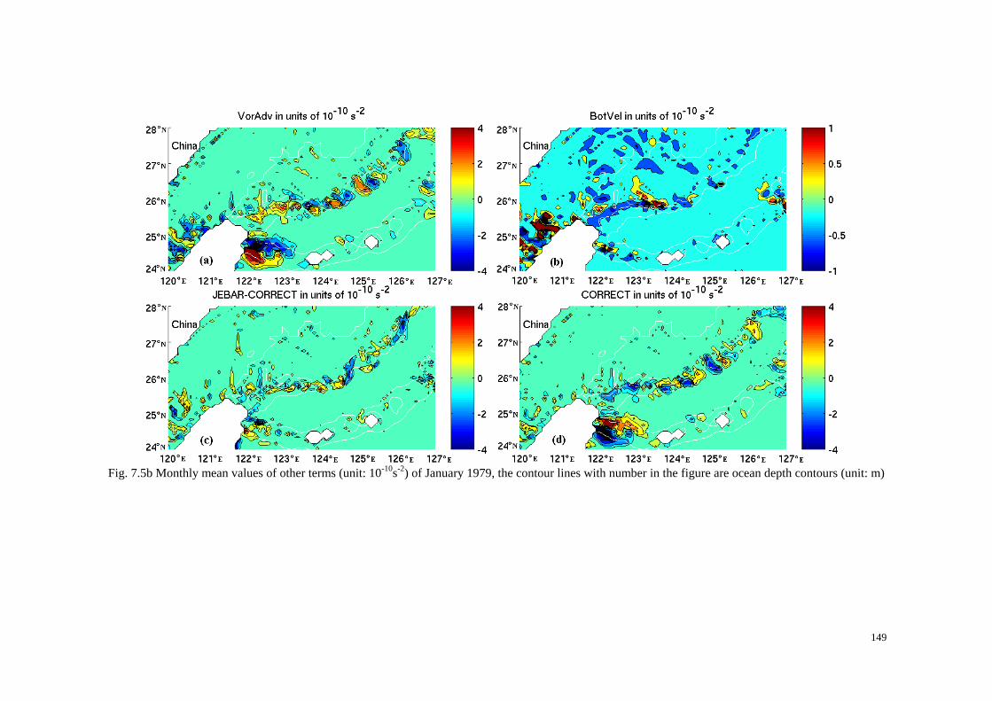
Fig. 7.5b Monthly mean values of other terms (unit: 10-10s-2) of January 1979, the contour lines with number in the figure are ocean depth contours (unit: m)

149

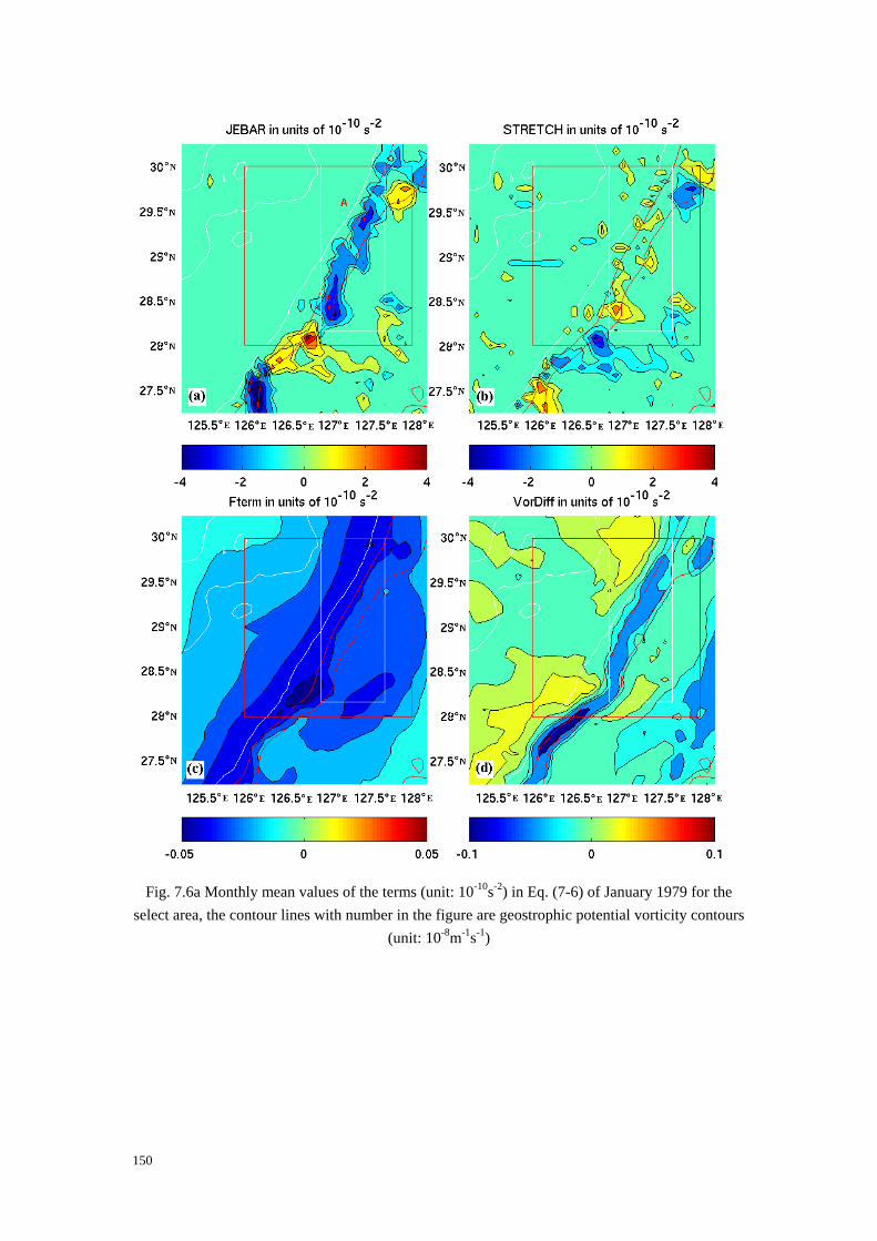
Fig. 7.6a Monthly mean values of the terms (unit: 10-10s-2) in Eq. (7-6) of January 1979 for the select area, the contour lines with number in the figure are geostrophic potential vorticity contours

(unit: 10-8m-1s-1)

150

Fig. 7.6b Monthly mean values of other terms (unit: 10-10s-2) of January 1979 for the select area, the contour lines with number in the figure are geostrophic potential vorticity contours (unit:

10-8m-1s-1)

151

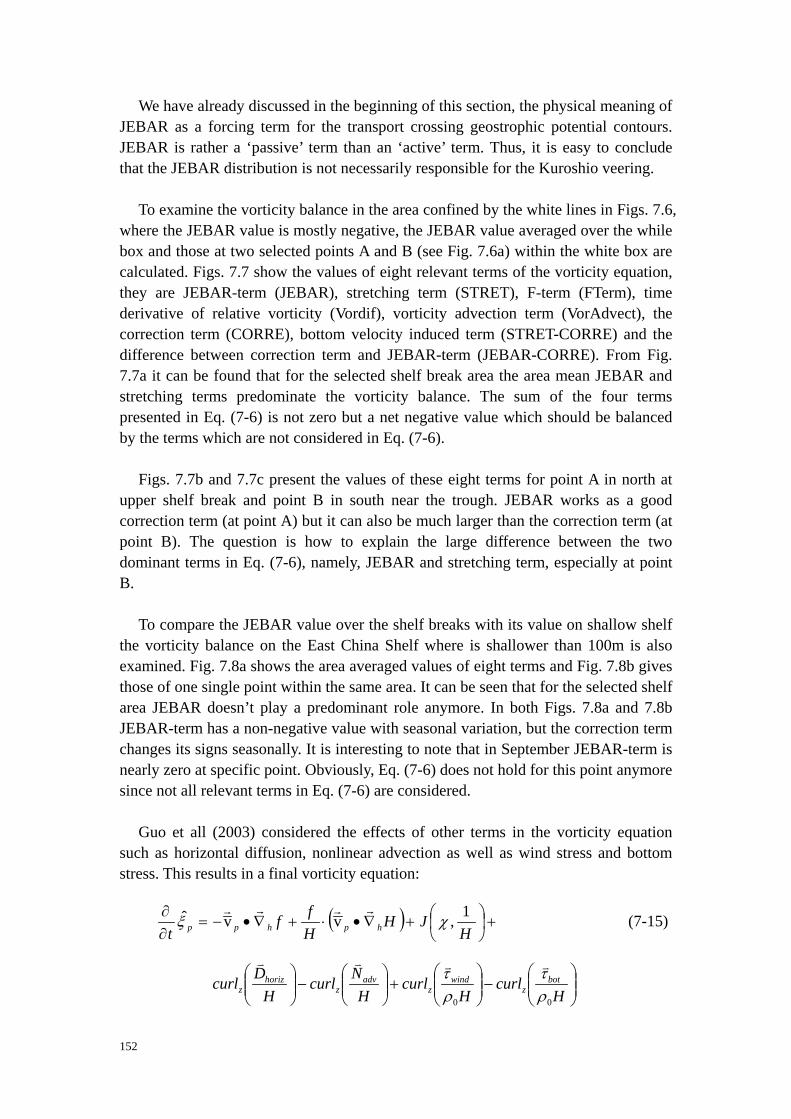
We have already discussed in the beginning of this section, the physical meaning of JEBAR as a forcing term for the transport crossing geostrophic potential contours. JEBAR is rather a ‘passive’ term than an ‘active’ term. Thus, it is easy to conclude that the JEBAR distribution is not necessarily responsible for the Kuroshio veering.

To examine the vorticity balance in the area confined by the white lines in Figs. 7.6,

where the JEBAR value is mostly negative, the JEBAR value averaged over the while box and those at two selected points A and B (see Fig. 7.6a) within the white box are calculated. Figs. 7.7 show the values of eight relevant terms of the vorticity equation, they are JEBAR-term (JEBAR), stretching term (STRET), F-term (FTerm), time derivative of relative vorticity (Vordif), vorticity advection term (VorAdvect), the correction term (CORRE), bottom velocity induced term (STRET-CORRE) and the difference between correction term and JEBAR-term (JEBAR-CORRE). From Fig. 7.7a it can be found that for the selected shelf break area the area mean JEBAR and stretching terms predominate the vorticity balance. The sum of the four terms presented in Eq. (7-6) is not zero but a net negative value which should be balanced by the terms which are not considered in Eq. (7-6).

Figs. 7.7b and 7.7c present the values of these eight terms for point A in north at

upper shelf break and point B in south near the trough. JEBAR works as a good correction term (at point A) but it can also be much larger than the correction term (at point B). The question is how to explain the large difference between the two dominant terms in Eq. (7-6), namely, JEBAR and stretching term, especially at point B.

To compare the JEBAR value over the shelf breaks with its value on shallow shelf

the vorticity balance on the East China Shelf where is shallower than 100m is also examined. Fig. 7.8a shows the area averaged values of eight terms and Fig. 7.8b gives those of one single point within the same area. It can be seen that for the selected shelf area JEBAR doesn’t play a predominant role anymore. In both Figs. 7.8a and 7.8b JEBAR-term has a non-negative value with seasonal variation, but the correction term changes its signs seasonally. It is interesting to note that in September JEBAR-term is nearly zero at specific point. Obviously, Eq. (7-6) does not hold for this point anymore since not all relevant terms in Eq. (7-6) are considered.

Guo et all (2003) considered the effects of other terms in the vorticity equation

such as horizontal diffusion, nonlinear advection as well as wind stress and bottom stress. This results in a final vorticity equation:

( ) +⎟⎠⎞

⎜⎝⎛+∇•⋅+∇•−=

∂∂

HJH

Hff

t hphpp1,vvˆ χξ

rrrr (7-15)

⎟⎟⎠

⎞⎜⎜⎝

⎛−⎟⎟

⎠

⎞⎜⎜⎝

⎛+⎟⎟

⎠

⎞⎜⎜⎝

⎛−⎟⎟

⎠

⎞⎜⎜⎝

⎛H

curlH

curlH

NcurlH

Dcurl botz

windz

advz

horizz

00 ρτ

ρτ vvvv

152

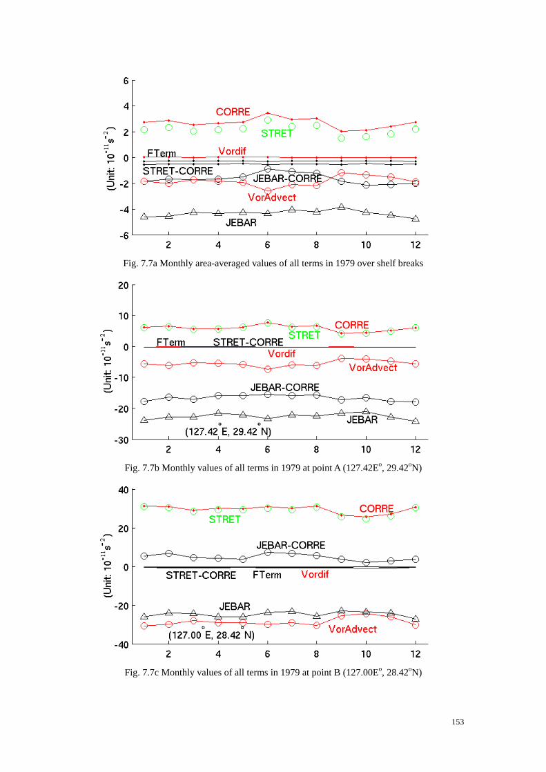
Fig. 7.7a Monthly area-averaged values of all terms in 1979 over shelf breaks

Fig. 7.7b Monthly values of all terms in 1979 at point A (127.42Eo, 29.42oN)

Fig. 7.7c Monthly values of all terms in 1979 at point B (127.00Eo, 28.42oN)

153

Fig. 7.8a Monthly area-averaged values in 1979 of all terms on shelf

Fig. 7.8b Monthly values of all terms in 1979 at point (124.67Eo, 27.92oN)

We can conclude from Guo et al. (2003) that after the model spin-up the depth-averaged horizontal diffusion and nonlinear advection terms contribute less to the vorticity balance in the area upstream the Kuroshio veering, and can even be neglected. The wind stress and the bottom stress play much more important roles. This could be the reason why a net positive value is needed to balance the difference between JEBAR and correction term.

To examine the general pattern of the JEBAR-term as well as those of other terms

on the East China Shelf, Figs. 7.9 to 7.13 give the monthly means of the four terms in Eq. (7-6) and the correction term for the year 1979.

For all five terms plotted in Figs. 7.9 to 7.13, their seasonal variability is strong in

the model domain especially in the shallow area, although the locations of maxima and minima are nearly stationary.

154

The JEBAR-term in Fig. 7.9 shows opposite signs over the trough west of Cheju Island in April (negative) and October (positive). In the Taiwan Strait and near the Changjiang river delta, the JEBAR-term has a strong seasonal variation. This means that due to the shallowness of these regions the density field exhibits a strong seasonal cycle. The heat flux and wind stress can influence the water at depth compared to the deep oceanic regions. The summer heating and winter cooling can seasonally reverse the density gradients in the shelf area. The variations of the Changjiang and Huanghe fresh water discharges can reduce the density gradient in winter and strengthen it in summer.

Only in shallow shelf areas the currents induced by the heat flux are comparable

with wind driven currents, in shelf breaks and in oceanic areas the surface ocean circulation is generally dominated by wind driven currents.

Fig. 7.10 and Fig. 7.11 show the correction term and the stretching term. The

difference between them is the bottom velocity induced term. From Fig. 7.3b, it can be seen that the maximum and minimum values of the bottom velocity induced term concentrate mainly in the Tsushima Strait, the central and the southern East China Shelf. Over most of the model domain the correction term and the stretching term have similar patterns and similar temporal variations. A striking feature is the existence of a positive correction band along the 100m depth contour near 30oN. At the northwestern corner of the whole domain, the correction term has an opposite sign in January and July. The central Huanghai trough again shows opposite signs in April and October.

We know that the stretching term and the bottom velocity induced term are

determined mainly by the variability of the circulation. Figs. 7.9 and 7.10 indicate that the correction term compensates most of the JEBAR term generated by depth-averaging of the vorticity equation. This point can also be proven by Fig. 7.3b.

The seasonal distribution of the F-term seems reasonable (Fig. 7.12). As we know,

it is a term only related to meridional velocity component. The northward currents will produce a negative F-term patch. The minimum values appear mainly along the Kuroshio path, in the Tsushima Strait and east of the Tokara Strait. The strongest F-term seasonal variations exist along the west and east Huanghai coast and are caused by the seasonal variations of the southward currents. The two seasonal positive patches west of the Tokara Strait are caused by the Kuroshio veering and the seasonal existence of the Kuroshio counter current.

The development of the time derivative of relative vorticity (Fig. 7.13) reaches

values which are at least one order of magnitude smaller than those of the JEBAR-term. The whole East China Shelf exhibits strong seasonal variations of relative vorticity. Maximum and minimum values are located east of the Taiwan Island, around the Tsushima Island and along the shelf breaks where the Kuroshio

155

passes the through. As we know, when the water column is squashed, it gets negative relative vorticity through the bottom friction layer. The band along the Kuroshio between depths of 200m and 1000m always gets negative relative vorticity. This is because the depth-averaged water column intrudes onto shelf and is squashed there. 7.4 Summary

As discussed in this chapter, JEBAR is nothing but a transport generating term. The causality is that JEBAR is an effect not a cause. According to its definition, the JEBAR-term describes the spatial strengths of the potential energy and the ocean depth contour gradients when they are not parallel to each other. The East China Shelf where the strong western boundary current Kuroshio and its branches interact with the complicated ocean topography provides an ideal case to study the physical processes behind JEBAR. It is indicated that JEBAR predominates where the shelf break, straits and fresh water discharges are located. Bottom slope is only one of the two prerequisites for JEBAR. Therefore, where the velocity is small the JEBAR is also small although the bottom slope is may be large.

JEBAR can be regarded as a forcing term only in a diagnostic calculation for

special ocean areas to produce an appropriate velocity field, such as around straits or shelf breaks with strong through-flows. Therefore, the bottom topography should be described realistically. For an idealized or simplified bottom topography JEBAR could give wrong results even with high resolution observations of the density field.

JEBAR can also be regarded as a correction term balancing the combined effect of

the stretching term and the bottom velocity induced term in order to keep the vorticity balance. A prerequisite for this case is that the velocity field is in geostrophic state. For these areas where heat flux, fresh water input and wind disturb the geostrophic balance, the correction term could even have the same sign as the JEBAR term. This is also the case if the bottom friction is relatively large. However, the correction term for most areas can be regarded as a ‘correction term’. For these areas where a part of JEBAR can not be balanced by the correction term, the JEBAR-term normally should be compensated by the effects of wind and bottom friction.

Compared to the JEBAR-term the term representing the time derivative of the

relative vorticity over the shelf break is fairly small. In the shallow shelf areas both of them have comparable magnitudes. This can be explained by the different characteristics of the velocity fields along shelf breaks and over the shallow shelf areas. In the latter the velocity fields are equally influenced by the heat flux, fresh water and wind stress, whereas along the shelf break the geostrophic balance is dominant.

156

Fig. 7.9a JEBAR-term distribution from Jan to Jun in 1979 (unit: 10-10s-2). The white lines are 100m, 200m and 1000m ocean depth contours.

157

Fig. 7.9b JEBAR-term distribution from Jul to Dec in 1979 (unit: 10-10s-2)

158

Fig. 7.10a Correction Term distribution from Jan to Jun in 1979 (unit: 10-10s-2)

159

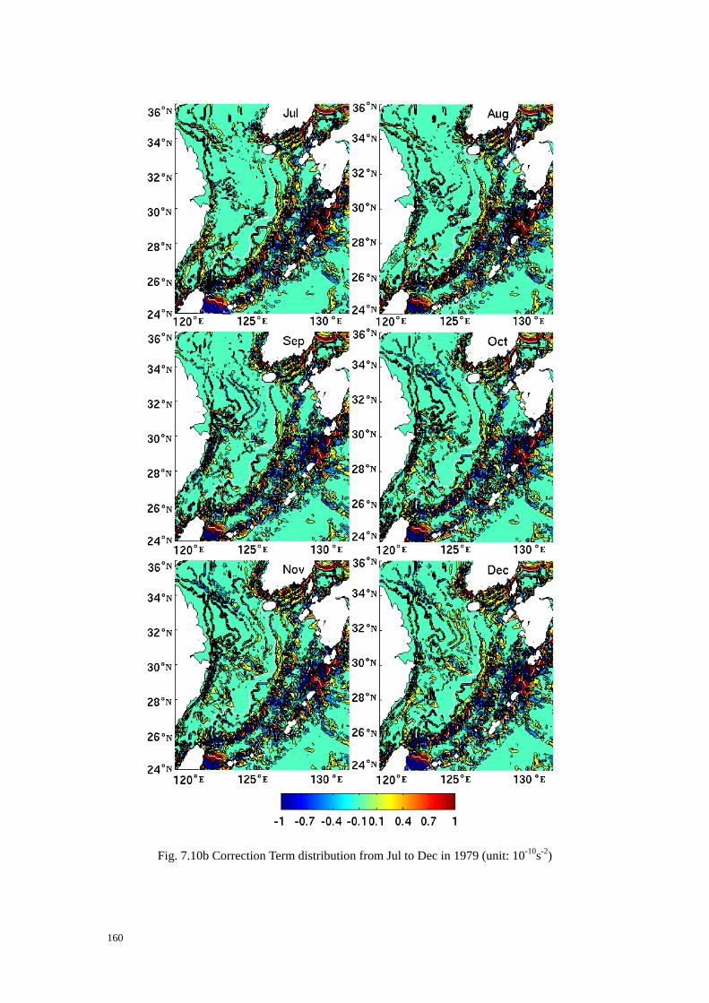
Fig. 7.10b Correction Term distribution from Jul to Dec in 1979 (unit: 10-10s-2)

160

Fig. 7.11a Stretching Term distribution from Jan to Jun in 1979 (unit: 10-10s-2)

161

Fig. 7.11b Stretching Term distribution from Jul to Dec in 1979 (unit: 10-10s-2)

162

Fig. 7.12a F-Term distribution from Jan to Jun in 1979 (unit: 10-10s-2)

163

Fig. 7.12b F-Term distribution from Jul to Dec in 1979 (unit: 10-10s-2)

164

Fig. 7.13a Time derivation of relative vorticity from Jan to Jun in 1979 (unit: 10-10s-2)

165

Fig. 7.13b Time derivation of relative vorticity from Jul to Dec in 1979 (unit: 10-10s-2)

166

Chapter 8 Summary and outlook

The East-Chinese Shelf (or North East Asian Regional seas – NEAR-seas) has the broadest shelf and the most complicated topography in the world. With the through-flow of one of the two largest western boundary currents: the Kuroshio, it provides an ideal case to investigate the water exchange mechanisms between shelf waters and oceanic waters, the variability of channel transports and the Joint Effect of Baroclinicity and Relief (JEBAR). In this Ph. D. study the 3-D baroclinic prognostic parallelised HAMburg Shelf Ocean Model (P-HAMSOM) was applied to the East-Chinese Shelf.

In the first chapter a review of earlier researches on the East-Chinese Shelf was

presented. Several scientific questions have been unanswered until the end of the 1990’s. For example, the variation of the Taiwan-Tsushima-Tsugaru Currents System in the East China Sea and the branch current of the Kuroshio northeast of the Taiwan Island and southwest of Kyushu. Due to limitations of computer resources and the lack of appropriate surface flux data, the earlier modelling works have been strongly confined to short-term case studies with simplified bottom descriptions.

In the second chapter the regional numerical hindcast model is described and a

numerical study with six hourly surface fluxes derived from the ERA40 reanalysis in the NEAR-seas from 1958 to 2001 is presented. The numerical model features a high resolution both vertically (30 model layers) and horizontally (five minutes by five minutes).

In the third chapter a systematic verification of the regional hindcast model is

described and its good performance in capturing the variations of the SST and velocity fields is documented. The validation data used spans from historical data of ship cruises to satellite remote sensing data.

In the fourth chapter the Kuroshio and its branch currents in the NEAR-seas are

investigated by an extensive analysis of the WOCE/SVP KRIG data from 1989 to 1999 which summarize the surface current pattern of the NEAR-seas. A tracer model has been designed to reproduce the trajectories of these Lagrangian drifters. The comparison serves as a further validation of the regional hindcast model. The achieved agreement is fairly good. For the first time the existence of a large eddy east of the Ryukyu archipelago was illustrated.

In the fifth and the sixth chapters the ocean temperature, salinity and current

variations have been analyzed based on the model output fields in the NEAR- seas. The characteristics of the climatological SST and SSS distribution are summarized. The existence of the HBCW (Huanghai Bottom Cold Water) was demonstrated and its structure during summer was described.

167

In the seventh chapter the vorticity balance in the NEAR-seas was examined and the JEBAR and its role for the East-Chinese Shelf systemically analyzed. According to this study, JEBAR-term is formulated as an arithmetically generated term in the vorticity equation. It can be a correction term to the vorticity balance only when the velocity field is approximately in a quasi-stationary state. Many earlier works have taken the JEBAR as a forcing mechanism for the currents in the real ocean; this is a misuse of the JEBAR term. The JEBAR can only be seen as a forcing term when the currents are examined in a pure diagnostic way. The distribution of maximum and minimum JEBAR values on the East-Chinese Shelf correlates well with location of the shelf break and straits. This guarantees the depth averaged vorticity balance in areas where strong currents occur. Here JEBAR as the dominating term is two orders of magnitude larger than the other vorticity terms. It plays a minor role in shallow shelf waters.

Outlook

Based on the discussion in the previous chapters, some modelling improvements should be performed in further numerical studies on the East-Chinese Shelf:

First the inclusion of tidal forcing would improve the model results in the shallow

waters of the East China Sea. Second a simulation with a nesting strategy will provide better dynamical

boundary inflows/outflows conditions at the open boundaries, especially an improvement in the sea level will include more realistically the far field effect of the northern Pacific for the hindcast.

Third as satellite derived data such as SST, wind and MSLA are widely available,

data assimilation techniques would be another approach to improve the quality of the hindcast.

Finally it is expected that an embedded ice model will improve the hindcast in the

northern Japan Sea.

168

Acknowledgements

Thanks should be given to Professor Dr. Jürgen Sündermann for his invitation and supervision. Only with his invitation I could be hosted in Hamburg as a visiting scholar.

Thanks should be given to Dr. Thomas Pohlmann. He gave and is giving me much

help not only for my Ph.D. study but also in organizing my life in Hamburg. He carefully corrects the text of the dissertation.

Thanks should be given to Dr. Wilfried Kuehn, Stiig Wilkenskjeld and Dr. Frank

Siegismund for their generous help in providing routines and corresponding discussions. Thanks should be given to Dr. Ilse Hamann, Tatyana Ilyina and Stiig Wilkenskjeld. They carefully read the text of the dissertation.

Thanks should be given to Dr. Peter Damm and our EDV team for the computer

technical support. Thanks should be given to many other colleagues in the Institute of Oceanography Hamburg, including our secretary team.

I gratefully acknowledge all these help I got till today. Thanks should be given to the joint support from China Scholarship Council in

China and the Hanns Seidel Stiftung in Germany. They sponsored and financed my visit to the Institute of Oceanography Hamburg from March 2002 to February 2004. Further financial aids have come from University of Hamburg from April 2004 to September 2004.

Thanks should be given to my group director in Ocean University of China,

Professor Dr. Dexing Wu. He encourages me to fulfill this further education in Germany.

Finally, I am very grateful for my family and friends who have given me constant

support.

Xueen CHEN November 22nd, 2004

169

List of abbreviations NEAR-seas North East Asian Regional seas. JEBAR the Joint Effect of Baroclinicity and Relief. ENSO the El Niño and Southern Oscillation. NPI North Pacific Index. PDO Pacific Decadal Oscillation. WOCE/SVP WOCE/Surface Velocity Program. (P-)HAMSOM (Parallelised) HAMburg Shelf Ocean Model. NCEP/NCAR National Center for Environmental Prediction/National Center for

Atmospheric Research.

List of tables Table 2.1 Six-hourly surface flux parameters of the model input. Table 3.1 Detailed information of selected tide gauges. Table 3.2 Location of temperature stations. Table 3.3 Information about the corresponding cruises. Table 4.1 Information on buoys released on 4 May 1992. Table 4.2 Information on buoys released on 24 Aug 1996. Table 4.3 Information on buoys released in May 1998. Table 4.4 Information on buoys released in April and June 1998. Table 5.1 Transport information across straits. Table 5.2 Transport information across the Ryukyu archipelago.

170

List of figures Fig. 2.1 Research area and the topography of our model area. Fig. 2.2a The yearly river discharges of Huanghe and Changjiang. Fig. 2.2b The climatological river discharges of Huanghe and Changjiang. Fig. 3.1 The distribution of selected tide gauges. Fig. 3.2 A 44-year comparison at tide gauge Naze. Fig. 3.3 A 33-year comparison at tide gauge Ishigaki. Fig. 3.4 A 7-year comparison at tide gauge Fukue. Fig. 3.5 A 5-year comparison at tide gauge Yonaguni. Fig. 3.6 Distribution of temperature stations. Fig. 3.7 Temperature comparison at Ishigaki from 1958 to 1999. Fig. 3.8 Temperature and salinity observations of cruises PN9606. Fig. 3.9 Simulated temperature of section PN9606. Fig. 3.10 Simulated salinity of section PN9606. Fig. 3.11 Simulated temperature of section PN9506. Fig. 3.12 Temperature observations of cruise PN9506. Fig. 3.13a Simulated salinity of section PN9506. Fig. 3.13b Salinity observations of cruise PN9506. Fig. 3.14a Simulated temperature of section TK9506. Fig. 3.14b Temperature observations of cruise TK9506. Fig. 3.15a Simulated salinity of section TK9506. Fig. 3.15b Salinity observations of cruise TK9506. Fig. 3.16a Monthly mean satellite Pathfinder SST of Aug 1992. Fig. 3.16b Monthly mean simulated SST of Aug 1992. Fig. 3.17a Monthly mean satellite Pathfinder SST of Oct 1992. Fig. 3.17b Monthly mean simulated SST of Oct 1992. Fig. 3.18a Monthly mean satellite Pathfinder SST of May 1993. Fig. 3.18b Monthly mean simulated SST of May 1993. Fig. 3.19a Monthly mean satellite absolute dynamic height of Sep 2001. Fig. 3.19b Monthly mean simulated sea levels of Sep 2001. Fig. 3.20a Monthly mean satellite absolute dynamic height of Dec 2001. Fig. 3.20b Monthly mean simulated sea levels of Dec 2001. Fig. 4.1.1 The mean velocity averages of the Pacific Ocean in February 2000. Fig. 4.2.1 The spatial release points distribution of the 250 buoys. Fig. 4.2.2 The temporal distribution of buoys release. Fig. 4.3.1 Temporal evolution at 21oN (left panel) and 24.3oN (right panel) of sea level

anomaly derived from satellite data. Fig. 4.3.2 Temporal evolution at 124oE (lower panel) and 127.3oE (upper panel) of sea level

anomaly derived from satellite data. Fig. 4.3.3 Temporal evolution at 144.5oE (lower panel) and 130oE (upper panel) of sea level

anomaly derived from satellite data. Fig. 4.3.4 Loops in the path of satellite drifting Buoy 9523909.

171

Fig. 4.3.5 Satellite derived sea level anomaly on 11 Dec 1995. Fig. 4.3.6 The selected buoys that describe the current pattern around the Taiwan Island. Fig. 4.3.7 Selected buoys describing the current pattern around Taiwan Island. Fig. 4.3.8a Some buoys that describe the eddy over northern Taiwan Island shelf. Fig. 4.3.8b The enlarged pictures of the buoys in Fig. 4.3.8a (time intervals of connecting

arrows: one day). Fig. 4.3.9a Selected buoys that describe the Kuroshio frontal eddies. Fig. 4.3.9b Selected buoys that describe the Kuroshio frontal eddies. Fig. 4.3.10 The anticyclonic motions of the Kuroshio southwest of Kyushu. Fig. 4.3.11a Selected buoys that indicate the Kuroshio branching current. Fig. 4.3.11b Selected buoys that indicate the Kuroshio branching current. Fig. 4.3.11c Selected buoys that indicate the Kuroshio branching current. Fig. 4.3.11d Selected buoys that indicate the Kuroshio branching current. Fig. 4.3.11e Selected buoys that indicate the Kuroshio branching current. Fig. 4.3.12a Selected buoys indicate exchange crossing Ryukyu archipelago. Fig. 4.3.12b Selected buoys indicate exchange crossing Ryukyu archipelago. Fig. 4.3.13 Selected buoys indicate exchange crossing Ryukyu archipelago. Fig. 4.4.1 Scheme of a tracer moving across model grid. Fig. 4.4.2 Contrast of the tracer trajectory simulation with and without random walk. Fig. 4.4.3 A simulated pattern of all the 115 buoys without diffusion. Fig. 4.4.4 The satellite traced routes of the buoys released in May 1992. Fig. 4.4.5 The satellite traced routes of the buoys released on 24 August 1996. Fig. 4.4.6 Simulated trajectories of the five buoys with a zero diffusion value. Fig. 4.4.7 Simulated paths distribution of Buoy 7700500. Fig. 4.4.8 Simulated paths of Buoy 7700498. Fig. 4.4.9 Simulated paths of Buoy 7700501. Fig. 4.4.10 Simulated paths of Buoy 9525138. Fig. 4.4.11 Simulated paths of Buoy 9525143. Fig. 4.4.12 The satellite-recorded routes of all nine buoys. Fig. 4.4.13 The simulated routes of all nine buoys. Fig. 4.4.14 Simulated 43-routes of Buoy 9715368. Fig. 4.4.15 Simulated routes of Buoy 9721219. Fig. 4.4.16 The satellite-recorded routes of buoys deployed in April and June. Fig. 4.4.17 Simulated routes of all seven Buoys in 1998. Fig. 4.5.1 Schematic current pattern. Fig. 5.1 The grid points and the section lines used to calculate the channel transport. Fig. 5.2a Distribution of the streamfunction based on a 6-year numeric integration of a

diagnostic study in units Sv (Hsueh et al. 1997). Fig. 5.2b Distribution of the streamfunction as climatological mean in October based on a

12-year fully prognostic run in units Sv (1990-2001). Fig. 5.3a Climatological monthly mean streamfunction in winter (February, units: Sv). Fig. 5.3b Climatological monthly mean stream function in summer (August, units: Sv). Fig. 5.4a The first EOF pattern (units: Sv). Fig. 5.4b The second EOF pattern (units: Sv).

172

Fig. 5.4c The third EOF pattern (units: Sv). Fig. 5.5a The first EOF PCs. Fig. 5.5b The second EOF PCs. Fig. 5.5c The third EOF PCs. Fig. 5.6 The climatological mean of the channels transport, details in text. Fig. 5.7 Volume transports derived by W. Teague et al. (2003). Fig. 5.8 Wavelet spectrum of the Taiwan Strait transport. Fig. 5.9 Wavelet spectrum of the east Taiwan channel transport. Fig. 5.10 Wavelet spectrum of PN line transport. Fig. 5.11 Wavelet spectrum of Tokara Strait transport. Fig. 5.12 Wavelet spectrum of middle Ryukyu archipelago channel transport. Fig. 5.13 Surface mean currents in the East China Sea derived from GEK data. Fig. 5.14a Daily mean velocity field on 15 February, 1994. Fig. 5.14b Daily mean velocity field on 15 August, 1994. Fig. 5.14c Daily sea surface elevation field on 15 February, 1994. Fig. 5.14d Daily sea surface elevation field on 15 August, 1994. Fig. 5.15 a Nov-Apr; b May-Oct (Lin et al. 2002). Fig. 5.16a The section distribution of velocity on 15 February. Fig. 5.16b The section distribution of velocity on 15 August. Fig. 5.17a The section distribution of velocity on 15 February. Fig. 5.17b The section distribution of velocity on 15 August. Fig. 5.18a The section distribution of velocity on 15 February. Fig. 5.18b The section distribution of velocity on 15 August. Fig. 5.19a The section distribution of velocity on 15 February. Fig. 5.19b The section distribution of velocity on 15 August. Fig. 6.1a A running average of the Niño 3.4 index from January 1958 to December 2001. Fig. 6.1b North Pacific index from 1958 to 2003. Fig. 6.1c Pacific Decadal Oscillation index from 1958 to 2003. Fig. 6.2a Simulated SST distribution in February in oC. Fig. 6.2b Simulated SST distribution in May in oC. Fig. 6.2c Simulated SST distribution in August in oC. Fig. 6.2d Simulated SST distribution in November in oC. Fig. 6.3a Simulated SSS distribution in February in psu. Fig. 6.3b Simulated SSS distribution in May in psu. Fig. 6.3c Simulated SSS distribution in August in psu. Fig. 6.3d Simulated SSS distribution in November in psu. Fig. 6.4a Time dependent SST variations across the PN section in oC. Fig. 6.4b Time dependent SSS variations across the PN section in psu. Fig. 6.5 Area-averaged yearly SST anomalies from 1958 to 2001 in the specified areas. Fig. 6.6a Salinity and temperature distribution in PN section in wintertime. Fig. 6.6b Salinity and temperature distribution in PN section in summertime. Fig. 6.7a Temperature and salinity at 50, 100 and 200m depth in wintertime. Fig. 6.7b Temperature and salinity at 50, 100 and 200m depth in summertime. Fig. 6.8 Lay out of temperature for each layer.

173

Fig. 6.9a Vertical salinity and temperature distribution across Huanghai in winter. Fig. 6.9b Vertical salinity and temperature distribution across Huanghai in summer. Fig. 7.1 Distribution of potential energy of selected area. Fig. 7.2a Monthly mean values of the JEBAR-term in January 1979. Fig. 7.2b Monthly mean values of the JEBAR-term in January 1979. Fig. 7.3a Monthly mean values of the terms of January 1979. Fig. 7.3b Monthly mean values of other terms of January 1979. Fig. 7.4a Monthly mean values of the terms of January 1979. Fig. 7.4b Monthly mean values of other terms of January 1979. Fig. 7.5a Monthly mean values of the terms of January 1979. Fig. 7.5b Monthly mean values of other terms of January 1979. Fig. 7.6a Monthly mean values of the terms of January 1979 for the select area. Fig. 7.6b Monthly mean values of other terms of January 1979 for the select area. Fig. 7.7a Monthly area-averaged values of all terms in 1979 over shelf breaks. Fig. 7.7b Monthly values of all terms in 1979 at point A. Fig. 7.7c Monthly values of all terms in 1979 at point B. Fig. 7.8a Monthly area-averaged values of all terms in 1979 at point value on shelf. Fig. 7.8b Monthly values of all terms in 1979 at point (124.67oE, 27.92oN). Fig. 7.9a JEBAR-term distribution from Jan to Jun. Fig. 7.9b JEBAR-term distribution from Jul to Dec. Fig. 7.10a Correction Term distribution from Jan to Jun. Fig. 7.10b Correction Term distribution from Jul to Dec. Fig. 7.11a Stretching Term distribution from Jan to Jun. Fig. 7.11b Stretching Term distribution from Jul to Dec. Fig. 7.12a F-Term distribution from Jan to Jun. Fig. 7.12b F-Term distribution from Jul to Dec. Fig. 7.13a Time derivation of relative vorticity from Jan to Jun. Fig. 7.13b Time derivation of relative vorticity from Jul to Dec.

174

List of symbols

zyx ,, spatial Cartesian coordinates eastward, northward and upward [m] kv

unity vector (positive upwards) t temporal coordinate [s]

wvu ,, velocities in zyx ,, -direction, respectively [m/s]

ppp wvu ,, pressure induced velocities in zyx ,, -direction, respectively [m/s]

pp pressure induced depth averaged velocities in

vu ,yx, - direction, respectively [m/s]

gg depth averaged geostrophic velocities in

vu ,yx, - direction, respectively [m/s]

pvr

vector of pp vu , [m/s]

pv~r

vector of pp vu ~,~ [m/s]

gv~r

vector of gg vu ~,~ [m/s] ζ sea surface elevation [m] H reference water depth [m] ρ density [kg/m3] ρ0 reference density [kg/m3] p pressure [Pa] p depth averaged pressure [Pa]

p0 sea surface pressure [Pa] f Coriolis parameter [s-1] g gravitational acceleration [m/s2]

pξ̂ relative vorticity of the depth averaged, [s-1] pressure induced velocities

pξ depth averaged pressure induced relative vorticity [s-1] χ potential energy for the water column [J] J Jacobi-operator [m-2]

h∇r

horizontal Nabla-operator [m-1]

pp vu ~,~ difference between depth averaged and the bottom velocity [m/s] both induced by the pressure gradient in yx, - direction, respectively

gg vu ~,~ difference between the geostrophic components of depth [m/s] averaged and the bottom velocity in yx, - direction, respectively

175

References

Akitomo, K., M. Ooi, T. Awaji, and K. Kutsuwada, 1996: Interannual variability of the Kuroshio transport in response to wind stress field over the North Pacific: Its relation to the path variation south of Japan. J. Geophys. Res., 101, 14057-14071.

Backhaus, J. O., 1985: A three-dimensional model for the simulation of shelf sea dynamics. Dt. Hydrogr. Z., 38, 165-187.

Backhaus, J. O., and D. Hainbucher, 1987: A finite difference general circulation model for shelf seas and its application to low frequency variability on the North European Shelf. In: Three dimensional models of marine and estuarine dynamics. Ed.: J. C. J. Nihoul und B. M. Jamart. Elsevier Oceanography Series 45, Elsevier, Amsterdam, 221-244.

Beardsley, R.C., R. Limeburner, H. Yu, and G. A. Cannon, 1985: Discharge of the Changjiang (Yangtze River) into the East China Sea. Continental Shelf Research, 4, 57-76.

Bryden, H. L., D. H. Roemmich and J. A. Church, 1991: Ocean Heat transport across 24N in the Pacific. Deep-Sea Research , 38, 297-324.

Cane, M. A., V. M. Kamenkovich, and A. Krupitsky, 1998: On the Utility and Disutility of JBAR. J. phys. Oceanogr., 28, 519-526.

Cessi, P., R. Condie, W. Young, 1990: Dissipative dynamics of western boundary currents. J. Mar. Res., 48, 677-700.

Chang, S., S. Jan, and K. Liu, 2001: Nutrient fluxes through the Taiwan Strait in Spring and Summer 1999. J. Oceanogr., 57, 47-53.

Chen, H., X. Yan, P. Shaw, and Q. Zheng, 1996: A numerical simulation of wind stress and topographic effects on a jet. J. Phys. Oceanogr., 26, 1769-1802.

Cho, Y., and K. Kim, 2000: Branching mechanism of the Tsushima Current in the Korean Strait J. Phys. Oceanogr., 30, 2788-2796.

Christopher, SA; Zhang, Jianglong, 2002: Shortwave Aerosol Radiative Forcing from MODIS and CERES observations over the oceans. Geophys. Res. Lett., 29, 1859.

Csanady, G. T., 1985: „Pycnobathic“ currents over the upper continental slope. J. phys. Oceanogr., 15, 306-315.

Ebuchi, N., and K. Hanawa, 2000: Mesoscale eddies observed by TOLEX-ADCP and TOPEX/POSEIDON altimeter in the Kuroshio recirculation region south of Japan. J. Oceanogr., 56, 43-57.

Endoh, N., and T. Hibiya, 2000: Numerical study of the generation and propagation of trigger meanders of the Kuroshio south of Japan. J. Oceanogr., 56, 58-70.

Fang, G., and B. Zhao and Y. Zhu, 1991: Oceanography of Asian Marginal Seas. Elsevier, 345-358.

Gibson, J. K., P. Kallberg, S. Uppala, A. Hernandez, A. Nomura, and E. Serrano, 1997: ERA description. ECMWF Re-Analysis Project Report Series, 1, 72 pp.

Gilson, G., and Roemmich, 2002: Mean and temporal variability in Kuroshio Geostrophic transport south of Taiwan (1993-2001). J. Oceanogr., 58, 183-195.

176

Greatbatch, R. J., A. F. Fanning, A. D. Goulding and S. Levitus, 1991: A diagnosis of interpentadal circulation changes in the North Atlantic, J. Geophys. Res., 96, 22009-22024.

Guan, Bingxian, 1996: Some observational evidences for the existence of two clockwise gyres on either side of Izu Ridge. J. Oceanogr. Huanghai Bohai Seas, 14, 1-9.

Guan, Bingxian, 2000: Inversion thermocline in coastal region north and east of Shandong Peninsula in winter and its relation to deep-bottom counter current. J. Oceanogr. Huanghai Bohai Seas, 18, 1-6.

Guo, Binghuo, 1992: Kuroshio frontal eddy, warm filament and warm ring in the East China Sea. J. Oceanogr. Huanghai Bohai Seas, 10, 10-19.

Guo, Binghuo, B. Wan, and Y. Tang, 1995: Wavelike features and evolution of the oceanic fronts in the East China Sea. J. Oceanogr. Huanghai Bohai Seas, 13, 1-10.

Guo, Binghuo, H. Lie, and J. H. Lee, 1998: Interaction of Kuroshio water and shelf water in the Tsushima Current region in summer. Acta Oceanologica Sinica., 20, 1-12.

Guo, Binghuo, Y. Tang, R. Ge, K. Lin, E. Zou, and X. Xiong, 2000a: Seasonal variations of the Taiwan Warm Current and the Kuroshio water intruded continental shelf. Acta Oceanologica Sinica., 22, suppl., 24-38.

Guo, Binghuo, E. Zou, X. Xiong, and W. Huang, 2000b: The seasonal variability of the sea water exchange between the Huanghai Sea and the East China Sea. Acta Oceanologica Sinica., 22, suppl., 13-23.

Guo, Binghuo, X. Hu, X. Xiong, and R. Ge, 2003: Study on interaction between the coastal water, shelf water and Kuroshio water in the Huanghai Sea and East China Sea. Acta oceanologica sinica., 22, 351-367.

Guo, X., and T. Yanagi, 1998: Three-dimensional structure of tidal current in the East China Sea and the Yellow Sea. J. Oceanogr., 54, 651-668.

Guo, X., H. Hukuda, Y. Miyazawa, and T. Yamagata, 2003: A triply nested ocean model for simulating the Kuroshio – roles of horizontal resolution on JEBAR. J. Phys. Oceanogr., 33, 146-169.

Hansen, D., and P. Poulain, 1996: Quality control and interpolations of WOCE/TOGA drifter data. Journal of Atmospheric and Oceanic Technology, 13, 900-909.

Hsueh, Y., and I.-C. Pang, 1989: Coastally trapped long waves in the Yellow Sea. J. Phys. Oceanogr., 5, 612-625.

Hsueh, Y., et al., 1996: On the branching of the Kuroshio west of Kyushu. J. Geophys. Res., 101, 3851-3857.

Hsueh, Y., and Dongliang Yuan, 1997: Currents, heat advection, and sea-level fluctuations in the Yellow Sea in winter of 1986. J. Phys. Oceanogr., 27, 2313-2326.

Hsueh, Y., J. Schultz, and W. Holland, 1997: The Kuroshio flow-through in the East China Sea: A numerical model. Prog. Oceanog., 39, 79-108.

Hsueh, Y., 2000: The Kuroshio in the East China Sea. J. Mar. Sys., 24, 131-139.

Huang, D., J. Su, and J. Backhaus, 1999: Modelling the seasonal thermal stratification and baroclinic circulation in the Bohai Sea. Continental Shelf Research, 19, 1485-1505.

177

Huthnance, J. M., 1984: Slope Currents and „JBAR“. J. phys. Oceanogr., 14, 795-810.

Ichikawa, H., and M. Chaen, 2000: Seasonal variation of heat and fresh water transport by the Kuroshio in the East China Sea. Journal of Marine System, 24, 119-129.

Ichikawa, K., 2001: Variation of Kuroshio in the Tokara strait induced by mesoscale eddies. J. Oceanogr., 57, 55-68.

Ichikawa, H., and R. Beardsley, 2002: The current system in the Yellow and East China Seas. J. Oceanogr., 58, 77-92.

Ichikawa, H., H. Nakamura, A. Nishina, and M. Higashi. 2004: Variability of Northeastward Current Southeast of Northern Ryukyu Islands. J. Oceanogr., 60, 351-363.

Imawaki, S., and H. Uchida, 2001: Satellite altimeter monitoring the Kuroshio transport south of Japan. Geophysical Research Letters, 28, 17-20.

Inoue, S., 1974: A simplified technique for measuring the flow speed in a water channel. Rep. Fish. Res. Lab. Kyushu Univ, 2, 79-85.

Isobe, A., 1994: Seasonal variation of the vertically averaged flow caused by the JEBAR effect in the Tsushima Strait. J. Oceanogr., 50, 617-633.

Isobe, A., 1997: The determinant of the volume transport distribution of the Tsushima Warm Current around the Tsushima Korea Strait. Continental Shelf Research, 17, 319-336.

Isobe, A., 1999a: On the origin of the Tsushima warm current and its seasonality. Continental Shelf Research, 19, 117-133.

Isobe, A., 1999b: The Taiwan-Tsushima warm current system: its path and the transformation of the water mass in the East China Sea. J. Oceanogr., 55, 185-195.

Isobe, A., 2000: Two-layer model on the branching of the Kuroshio southwest of Kyushu, Japan. J. Phys. Oceanogr., 30, 2461-2476.

Isoda, Y., T. Yanagi, H-J. Lie, 1991: Sea-level variations with a several-day period along the southwestern Japan Sea coast. Continental Shelf Research, 11, 167-182.

Jacobs, G. A., H. Hurlburt, J. Kindle, E. Metzger, J. Mitchell, W. Teague, and A. Wallcraft, 1994: Decade-scale trans-Pacific propagation and warming effects of an El Nino anomaly. Nature, 370, 360-363.

Jacobs, G. A,, P. J. Hogan, and K. R. Whitmer, 1999: Effects of eddy variability on the circulation of the Japan/East Sea. J. Oceanogr., 55, 247-256.

Johns, W. E., T. N. Lee, D. Zhang, R. Zantopp, C. T. Liu and Y. Yang, 2001: The Kuroshio east of Taiwan: Moored transport observations from the WOCE PCM-1 array. J. Phys. Oceanogr., 31, 1031-1053.

Johnson, R.H., and P.E. Ciesielski, 2000: The SCSMEX/GAME sounding networks and the onset of the 1998 Asian Summer Monsoon. Proceedings of the 4th Conference on East Asian and Western Pacific Meteorology and Climate, Hangzhou.

Johnson, D. R., and W. J. Teague, 2002: Observations of the Korea Strait bottom cold water. Continental Shelf Research, 22, 821-831.

Kalnay, E. and Z. Toth, 1996: The breeding method. Proceedings, 1995 ECMWF Seminar on Predictability, 1, European Centre for Medium-Range Weather Forecasts, 69-82.

178

Kawabe, M., 1982: Branching of the Tsushima Current in the Japan Sea. Part II. Numerical experiment. J. Oceanogr. Soc. Jap., 38, 183-192.

Kawabe, K., 1995: Variations of current path, velocity and volume transport of the Kuroshio in relation with the large meander. J. Phys. Oceanogr., 25, 3103-3117.

Kawamura, H., and P. Wu, 1998: Formation mechanism of Japan Sea Proper Water in the flux center off Vladivostok. J. Geophys. Res., 103, 21611-21622.

Kim, K., and R. Legeckis, 1986: Branching of the Tsushima Current in 1981-83. Prog. Oceanog., 17, 265-276.

Kochergin, 1987: Three-dimensional prognostic models. Three-dimensional coastal ocean models, (American Geophysical Union), 4, 201-208.

Lee, H., K. Jung, J. So, and J. Chung, 2002: A 3-dimensional mixed finite-difference Galerkin function model for the oceanic circulation in the Yellow Sea and the East China Sea in the presence of M2 tide. Continental Shelf Research, 22, 67-91.

Lee, S., and R. Beardsley, 1999: Influence of stratification on residual tidal currents in the Yellow Sea. J. Geophys. Res., 104, 15679-15701.

Lee, T. N., and L. P. Atkinson, R. Legeckis, 1981: Observations of a Gulf Stream frontal eddy on the Georgia continental shelf, April 1977. Deep-Sea Research, 28, 347-378.

Levitus, S., 1982: Climatological atlas of the World Ocean. NOAA Prof. Pap., Noaa/Erl, Princeton, NJ (USA), 190 pp.

Levitus, S., and O'Brien, 1998: The World Ocean Database 1997 -- new opportunities for objective analysis of oceanographic data. Intergovernmental Oceanographic Comm., Paris (France); National Oceanic and Atmospheric Administration (USA); EC Marine Science and Technology (DGXII); Marine Institute, Irish Marine Data Centre (Ireland).

Li, Kunping, X. Fang, L. Liu, and X. Zeng, 1993: Response of the sea level changes to variabilities of the Kuroshio. J. Oceanogr. Huanghai Bohai Seas, 11, 30-37.

Liao, Qiyu, B. Guo, and Z. Liu, 2001: Analysis of direction change mechanism of the Changjiang River diluted water in summer. J. Oceanogr. Huanghai Bohai Seas, 19, 19-25.

Lie, H., 1986: Summertime hydrographic features in the southeastern Hwanghae. Prog. Oceanog., 17, 229-242.

Lie, H., C. Cho, J. Lee, S. Lee, and Y. Tang, 2000: Seasonal variation of the Cheju warm current in the northern East China Sea. J. Oceanogr., 56, 197-211.

Lin, Kui, Y. Tang, and B. Guo, 1995a: Study on velocity structure and volume transport of the Kuroshio in the Tokara Strait. Oceanologia et Limnologia Sinica., 26, 247-253.

Lin, Kui, Z. Chen, B. Guo, and Y. Tang, 1995b: Seasonal transport and exchange between the Kuroshio water and shelf water. J. Oceanogr. Huanghai Bohai Seas, 13, 1-8.

Liu, C. T., S. P. Cheng, and W. S. Chuang, 1998: Mean Structure and Transport of Taiwan Current. Acta Oceanographica. Taiwanica., 36, 159-176.

Lin, Kui, Y. Tang, and B. Guo, 2002: An analysis on observational surface and upper layer current in the Huanghai Sea and the East China Sea. Acta oceanologica sinica., 24, 9-19.

Liu, Yonggang, and Y. Yuan, 1998: Variability of the Kuroshio in the East China Sea in 1992. Acta

179

Oceanologica Sinica., 20, 1-11.

Liu, Yonggang, and Y. Yuan, 1999a: Variability of the Kuroshio inn the East China Sea in 1995. Acta Oceanologica Sinica., 18, 459-475.

Liu, Yonggang, and Y. Yuan, 1999b: Variability of the Kuroshio in the East China Sea in 1993 and 1994. Acta Oceanologica Sinica., 21, 15-29.

Masuda. A., 1982: An interpretation of the bimodal character of the stable Kuroshio path. Deep-Sea Res., 31, 61-66.

McCartney, M. S., 1982: The subtropical recirculation of Mode waters. J. Mar. Res., 40, 427-464.

Mellor, G. L., and T. Yamada, 1974: A hierarchy of turbulence closure models for planetary boundary layers. J. Atmos. Sci., 31, 1791-1806.

Mertz, G., and D. G. Wright, 1992: Interpretations of the JEBAR Term. J. Phys. Oceanogr., 22, 301-305.

Miao, Yutian, H. Yu, D. He, and C. Wang, 1998: Characteristics of water type distribution and seasonal variation in the Southern East China Sea. Marine science bulletin, 17, 1-9.

Miita, T., and K. Kawatate, 1986: Trajectories of drift bottles in the Tsushima Strait. Prog. Oceanog., 17, 255-263.

Morimoto, A., T. Yanagi, and A. Kaneko, 2000: Eddy field in the Japan Sea derived from satellite altimetric data. J. Oceanogr., 56, 449-462.

Myers, P.G., A. F. Fanning, and A. J. Weaver, 1996: JEBAR, bottom pressure torque, and Gulf Stream separation. J. Phys. Oceanogr., 26, 671-683.

Naimie, C., C. Blain, and D. Lynch, 2001: Seasonal mean circulation in the Yellow Sea – a model-generated climatology. Continental Shelf Research, 21, 667-695.

Nitani, H., 1972: Beginning of the Kuroshio. Kuroshio: Its Physical Aspects. ed. by H. Stommel and K. Yoshida, Univ. of Tokyo Press, Tokyo, 129-163.

Oka, E., and M. Kawabe, 2003: Dynamic structure of the Kuroshio south of Kyushu in relation to the Kuroshio path variations. J. Oceanogr., 59, 595-608.

Onishi, M., and K. Ohtani, 1997: Volume transport of the Tsushima warm current, west of Tsugaru strait bifurcation area. J. Oceanogr., 53, 27-34.

Pan, Y., K.Wang, and S. Huang,1997: Analysis on the path of transportation and diffusion of Changjiang diluted water. Donghai Mar. Sci., 15, 25-34.

Park, K., J. Chung, 1999: Spatial and temporal scale variations of sea surface temperature in the East Sea using NOAA/AVHRR data. J. Oceanogr., 55, 271-288.

Park, W., and I. Oh, 2000: Interannual and interdecadal variations of sea surface temperature in the east Asian Marginal Seas. Prog. Oceanog., 47, 191-204.

Park, Y., 1986: Water characteristics and movement in the Yellow Sea Warm Current in summer. Prog. Oceanog., 17, 243-254.

Park, Y-C., Y-H. Kim, C-S. Lee, and K-B Lee, 1991: Identification of spilled oils in the marine environment by fluorescence fingerprints and library search system. J. Oceanol. Soc. Korea, 26, 295-303.

180

Pedlosky, J.,1987: An inertial theory of the equatorial undercurrent. J. Phys. Oceanogr., 17, 1978-1985.

Pohlmann, T., 1991. Investigation of hydrodynamic and thermodynamic processes in the North Sea using a threedimensional numerical model. Ber. Zent. Meeres-Klimaforsch. Univ. Hamb., 23, 116 pp.

Pohlmann, T., 1996a: Predicting the Thermocline in a Circulation Model of the North Sea --Part I: Model Description, Calibration and Verification. Continental Shelf Research, 16, 131-146.

Pohlmann, T., 1996b: Calculating the annual cycle of the vertical eddy viscosity in the North Sea with a three-dimensional circulation model. Continental Shelf Research, 16, 147-161.

Pohlmann, T., 1999: Discussion of the JBAR term – Derivation, Interpretation and Application to the Northeastern Atlantic Shelf. Report of European Communities, 1999.

Pohlmann, T., 2003: Eine Bewertung der hydro-thermodynamischen Nordseemodellierun. Berichte aus dem Zentrum fuer Meeres- und Klimaforschung. Reihe B, 46, 146 S.

Qiu, B., T. Toda, and N. Imasato, 1990: On Kuroshio front fluctuations in the East China Sea using satellite and in situ observational data. J. Geophys. Res., 95, 18191-18204.

Qiu, B., and T. Joyce, 1992: Interannual variability in the mid- and low-latitude western Pacific. J. Phys. Oceanogr., 22, 1062-1079.

Qiu, B., 2000: Interannual variability of the Kuroshio extension system and its impact on the wintertime SST field. J. Phys. Oceanogr., 30, 1486-1502.

Qiu, B., and W. Miao, 2000: Kuroshio path variation south of Japan: Bimodality as a self-sustained internal oscillation, J. Phys. Oceanogr., 30, 2124–2137.

Qiu, B., 2002: The Kuroshio extension system: its large-scale variability and role in the mid-latitude ocean atmosphere interaction. J. Oceanogr., 58, 57-75.

Riedlinger, S., and R. Preller, 1995: Validation test report for the Yellow Sea shallow water analysis and forecast system. Draft NRL Report, Stennis Space Center, MI.

Roemmich, D. and T. McCallister, 1989: Large-scale circulation of the North Pacific ocean. Progr. in Oceanogr., 22, 171-204.

Sager, G., 1968: Atlas der Gezeitenströme für die Nordsee, den Kanal und die Irische See. Seehydrog. Dienst d. DDR Rostock, 58 S.

Sarkisyan, A. S., and V. F. Ivanov, 1971: The combined effect of baroclinicity and bottom relief as an important factor in the dynamics of ocean currents (AGU translation). Izv. Acad. Sci. USSR, Atmos. Oceanic Phys., 173-188.

Sarkisyan, A. S., 1977: The diagnostic calculation of large-scale oceanic circulation. The Sea, Ed. E. D. Goldberg, VI, Marine Modelling, 363-458.

Schrum, C., 1997: Thermohaline stratification and instabilities at tidal mixing fronts - Results of an eddy resolving model for the German Bight. Continental Shelf Research, 17, 689-716.

Schrum, C., and J. Backhaus, 1999: Sensitivity of atmosphere-ocean heat exchange and heat content in the North Sea and the Baltic Sea. Tellus (A Dyn. Meteorol. Oceanogr.), 51a, 526-549.

Seung, Y. H., 1999: A geostrophic adjustment model of shelfward intrusion of oceanic upper water

181

across a depth discontinuity: implication to the Kuroshio region. Continental Shelf Research, 19, 247-269.

Shu, Lianghua, B. Guo, and Z. Chen, 1993: A diagnostic model for calculating current on shelf slope. J. Oceanogr. Huanghai Bohai Seas, 11, 19-29

Smith, W., and D. Sandwell, 1997: Global sea floor topography from satellite altimetry and ship depth soundings. Science (Wash.), 277, 1956-1962.

Smith, R. D., M. E. Maltrud, F. O. Bryan, and M. W. Hecht, 2000: Numerical simulation of the north Atlantic Ocean at 1/10°. J. Phys. Oceanogr., 30, 1532–1561.

Song, Wanxian, and B. Guo, 1996: The structures of current velocity, temperature and salinity on the 129 degree E section west of Kyushu. Oceanologia et Limnologia Sinica., 27, 538-545.

Stronach, J. J. Backhaus, and T. Murty, 1993: An update on the numerical simulation of oceanographic processes in the waters between Vancouver Island and the mainland: The GF8 model. Oceanogr. Mar. Biol. Annu. Rev., Ucl Press, London (UK), 31, 1-86.

Sugimoto, T., S. Kimura, and K. Miyaji, 1988: Meander of the Kuroshio front and current variability in the East China sea. J. Oceanogr. Soc. Japan, 44, 125-135.

Sun, Xiangping, 1987: Analysis of the surface path of the Kuroshio in the East China Sea. Essays on the Investigation of the Kuroshio, 1-14.

Sun, Xiangping, Y. Wang, H. Xu, and Q. Yuan, 1991: The path, velocity and volume transport of the Kuroshio during 1986-1988. State Oceanic Adm., Beijing (China). Essays on the Investigation of Kuroshio, 3, 48-59

Sun, Xiangping, and S. Xiu, 2002: Characteristics of the cold water body northeast of Taiwan. J. Oceanogr. Huanghai Bohai Seas, 20, 1-10.

Talley, L. D., 1993: Distribution and formation of North Pacific intermediate water. J. Phys. Oceanogr., 23, 517-537.

Tang, T. Y., J. C. Ma, 1995: A note on the accuracy of shipboard ADCP on Ocean Researcher. I. Acta Oceanographic Taiwanica., 34, 71-81.

Tang, Y. T., J. H. Tai, and Y. J. Yang, 2000: The flow pattern north of Taiwan and the migration of the Kuroshio. Continental Shelf Research, 20, 349-371.

Tang, Yuxiang, 1992: On regional difference of the Kuroshio front in the East China Sea. J. Oceanogr. Huanghai Bohai Seas, 10, 1-9.

Tang, Yuxiang, 1995: Preliminary study on classification of oceanic fronts in East China Sea. J. Oceanogr. Huanghai Bohai Seas, 13, 16-22.

Tang, Yuxiang, 1996: Distributional features and seasonal variations of temperature fronts in the East China Sea. Oceanologia et Limnologia Sinica., 27, 436-444.

Teague, W. J., G. A. Jacobs, 2000: Current observations on the development of the Yellow Sea Warm Current. J. Geophys. Res., 105, 3401-3411.

Teague. W. J., G. A. Jacobs, D. S. Ko, T. Y. Tang, K. Chang, and M. Suk, 2003: Connectivity of the Taiwan, Cheju and Korea straits. Continental Shelf Research, 23, 63-77.

Toba, Y., and H. Murakami, 1998: Unusual behavior of the Kuroshio current system from Winter 1996 to Summer 1997 revealed by using ADEOS-OCTS and other data. J. Oceanogr., 54,

182

465-478.

Toba, Y., and H. Murakami, 1999: New progress of the Kuroshio current system research by using ADEOS-OCTS. Adv. Space Res., 25, 967-968.

Trenberth, and Hurrell, 1994: Decadal Atmosphere-Ocean Variations in the Pacific. Climate Dynamics, 9, 303-319.

Tseng, C., C. Lin, S. Chen, and C. Shyu, 2000: Temporal and spatial variations of sea surface temperature in the East China Sea. Continental Shelf Research, 20, 373-387.

Tsuchiya, M., 1982: On the Pacific upper-water circulation. J. Mar. Res., 40, 777-799.

Valle-Levinson, A., and T. Matsuno, 2003: Tidal and subtidal flow along a cross-shelf transect on the East China Sea. J. Oceanogr., 58, 77-92.

Wan, Bangjun, and B. Guo, 1992: Mixing and exchange of the Kuroshio water and continental shelf water in the area north of Taiwan. J. Oceanogr. Huanghai Bohai Seas, 10, 1-9.

Wan, Bangjun, B. Guo, and Y. Tang, 1994: Current structure along cross-Kuroshio front section in the East China Sea. Oceanologia et limnologia sinica., 25, 652-659.

Waseda, T., H. Mitsudera, B. Taguchi, and Y. Yoshikawa, 2002: On the eddy-Kuroshio interaction: Evolution of the mesoscale eddy, J. Geophys. Res., 107, 3088-4002.

Waseda, T., and H. Mitsudera, 2003: On the eddy-Kuroshio interaction: Meander formation process. J. Geophys. Res., 108, 3220-3236.

Wyrtki K., 1961: Physical oceanography of the Southeast Asian waters. NAGA Report, 2, Scientific Results of Marine Investigations of the South China Sea and the Gulf of Tailand, Scripps Institution of Ocranography, La Jolla, California, 195 pp.

Wyrtki, K., 1965: The annual and semiannual variation of sea surface temperature in the North Pacific Ocean. Limnol. Oceanogr., 10, 307-313.

Xu, Qichun, Z. Wang, and Q. Liu, 1993: The variation of wind stress in northern Pacific and its relationship to Kuroshio meander and El-Nino event. J. Ocean Univ. Qingdao, 23, 21-28.

Yamagata, T., Y. Shibao, and S. Umatani, 1985: Interannual variability of the Kuroshio Extension and its relation to the Southern Oscillation/El Niño. J. Oceanogr. Soc. Japan, 41, 274-281.

Yanagi, T., T. Shimizu, and H. Lie, 1998: Detailed structure of the Kuroshio frontal eddy along the shelf edge of the East China Sea. Continental Shelf Research, 18, 1039-1056.

Yang, Y., C. Liu, and J. Hu, 1999: Taiwan Current and Impinging Eddies. J. Oceanogr., 55, 609-617.

Yasuda, K. Okuda and M. Hirai, 1992: Evolution of a Kuroshio Warm-Core Ring - Variability of the hydrographic structure. Deep-Sea Res., 39, 131-161.

Yoon, J. H., and I. Yasuda, 1986: Dynamics of Kuroshio large meander: two-layer model. J. Phys. Oceanogr., 17, 66-81.

Yuan, Y., et al., 1998: The Kuroshio East of Taiwan and in the East China Sea and the Currents East of Ryukyu Islands during Early Summer of 1996. J. Oceanogr., 54, 217-226.

Yuan, Y., Y., Liu, and H. Wang, 2000: The Kuroshio east of Taiwan and in the East China Sea in July 1997. La Mer, 38, 173-178.

183

Zhao, Baoren, and G. Fang, 1991: Estimation of water volume transports through the main strains of the East China Sea. Acta oceanologica sinica., 10, 1-14.

Zhao, Yongping, and G. A. Mcbean, 1995: Air-sea interaction between the Kuroshio region marine heating anomaly and Northern Hemisphere atmospheric circulation. Oceanologia et Limnologia Sinica., 26, 383-388.

Zhao, Yongping, Y. Chen, and R. Ja, 1996: Air-sea interaction in the mid-latitude in winter and prediction of flood and lower reaches of Changjiang River. Inst. Oceanol. Acad. Sin., 37, 19-24.

Zhu, et al., 2003: The Northeastward Current Southeast of Okinawa Island Observed During November 2000 to August 2001. Geophysical Research Letters, 30, 1071-1085.

184

Erklärung

Ich versichere ausdrücklich, dass ich die Arbeit selbständig und ohne fremde Hilfe verfasst, andere als die von mir angegebenen Quellen und Hilfsmittel nicht benutzt und die aus den benutzten Werken wörtlich oder inhaltlich entnommenen Stellen einzeln nach Ausgabe (Auflage und Jahr des Erscheinens), Band und Seite des benutzten Werkes kenntlich gemacht habe. Ich habe bis zum diesen Zeitpunkt noch keinen Promotionsversuch unternommen.

Xueen Chen Hamburg, den 22. November 2004

185