Analysis of the Cholesky Method with Iterative Reﬁnement ...eprints.ma.man.ac.uk/1123/01/covered/MIMS_ep2008_70.pdf · Analysis of the Cholesky Method with Iterative Reﬁnement

Analysis of the Cholesky Method with IterativeRefinement for Solving the Symmetric Definite

Generalized Eigenproblem

Davies, Philip I. and Higham, Nicholas J. and Tisseur,Françoise

2001

MIMS EPrint: 2008.70

Manchester Institute for Mathematical SciencesSchool of Mathematics

The University of Manchester

Reports available from: http://eprints.maths.manchester.ac.uk/And by contacting: The MIMS Secretary

School of Mathematics

The University of Manchester

Manchester, M13 9PL, UK

ISSN 1749-9097

http://eprints.maths.manchester.ac.uk/

ANALYSIS OF THE CHOLESKY METHOD WITHITERATIVE REFINEMENT FOR SOLVING THE

SYMMETRIC DEFINITE GENERALIZED EIGENPROBLEM∗

PHILIP I. DAVIES† , NICHOLAS J. HIGHAM† , AND FRANCOISE TISSEUR†

SIAM J. MATRIX ANAL. APPL. c© 2001 Society for Industrial and Applied MathematicsVol. 23, No. 2, pp. 472–493

Abstract. A standard method for solving the symmetric definite generalized eigenvalue problemAx = λBx, where A is symmetric and B is symmetric positive definite, is to compute a Choleskyfactorization B = LLT (optionally with complete pivoting) and solve the equivalent standard sym-metric eigenvalue problem Cy = λy, where C = L−1AL−T . Provided that a stable eigensolver isused, standard error analysis says that the computed eigenvalues are exact for A+∆A and B+∆Bwith max(‖∆A‖2/‖A‖2, ‖∆B‖2/‖B‖2) bounded by a multiple of κ2(B)u, where u is the unit round-off. We take the Jacobi method as the eigensolver and give a detailed error analysis that yieldsbackward error bounds potentially much smaller than κ2(B)u. To show the practical utility of ourbounds we describe a vibration problem from structural engineering in which B is ill conditionedyet the error bounds are small. We show how, in cases of instability, iterative refinement based onNewton’s method can be used to produce eigenpairs with small backward errors. Our analysis andexperiments also give insight into the popular Cholesky–QR method, in which the QR method isused as the eigensolver. We argue that it is desirable to augment current implementations of thismethod with pivoting in the Cholesky factorization.

Key words. symmetric definite generalized eigenvalue problem, Cholesky method, Choleskyfactorization with complete pivoting, Jacobi method, backward error analysis, rounding error anal-ysis, iterative refinement, Newton’s method, LAPACK, MATLAB

AMS subject classification. 65F15

PII. S0895479800373498

1. Introduction. The symmetric definite generalized eigenvalue problem

Ax = λBx,(1.1)

where A,B ∈ Rn×n are symmetric and B is positive definite, arises in many applica-

tions in science and engineering [4, chapter 9], [16]. An important open problem isto derive a method of solution that takes advantage of the structure and is efficientand backward stable. Such a method should, for example, require half the storageof a method for the generalized nonsymmetric problem and produce real computedeigenvalues.

The QZ algorithm [18] can be used to solve (1.1). It computes orthogonal matricesQ and Z such that QTAZ is upper quasi-triangular and QTBZ is upper triangular.This method is numerically stable but it does not exploit the special structure ofthe problem and so does not necessarily produce real eigenpairs in floating pointarithmetic.

∗Received by the editors June 9, 2000; accepted for publication (in revised form) by M. Chu April11, 2001; published electronically September 7, 2001.

http://www.siam.org/journals/simax/23-2/37349.html†Department of Mathematics, University of Manchester, Manchester, M13 9PL, England

([email protected], http://www.ma.man.ac.uk/˜ieuan/, [email protected], http://www.ma.man.ac.uk/˜higham/, [email protected], http://www.ma.man.ac.uk/˜ftisseur/). The workof the first author was supported by an Engineering and Physical Sciences Research Council CASEPh.D. Studentship with NAG Ltd. (Oxford) as the cooperating body. The work of the second authorwas supported by Engineering and Physical Sciences Research Council grant GR/L76532 and a RoyalSociety Leverhulme Trust Senior Research Fellowship. The work of the third author was supportedby Engineering and Physical Sciences Research Council grant GR/L76532.

472

SYMMETRIC DEFINITE GENERALIZED EIGENPROBLEM 473

A method that potentially has the desired properties has recently been proposedby Chandrasekaran [3], but the worst-case computational cost of this algorithm isnot clear.

A standard method, apparently first suggested by Wilkinson [25, pp. 337–340], be-gins by computing the Cholesky factorization, optionally with complete pivoting [12,section 4.2.9], [14, section 10.3],

ΠTBΠ = LD2LT ,(1.2)

where Π is a permutation matrix, L is unit lower triangular, and D2 = diag(d2i ) is

diagonal. The problem (1.1) is then reduced to the form

Cy ≡ D−1L−1ΠTAΠL−TD−1y = λy, y = DLTΠTx.(1.3)

Any method for solving the symmetric eigenvalue problem can now be applied toC [6], [19]. In LAPACK’s xSYGV driver, (1.1) is solved by applying the QR algo-rithm to (1.3). MATLAB 6’s eig function does likewise when it is given a symmetricdefinite generalized eigenproblem. As is well known, when B is ill conditioned numer-ical stability can be lost in the Cholesky-based method. However, it is also knownthat methods based on factorizing B and converting to a standard eigenvalue prob-lem have some attractive features. In reference to the method that uses a spectraldecomposition of B, Wilkinson [25, p. 344] states that

In the ill-conditioned case the method of §68 has certain advantagesin that “all the condition of B” is concentrated in the small elementsof D. The matrix P of (68.5) [our C in (1.3)] has a certain numberof rows and columns with large elements (corresponding to small dii)and eigenvalues of (A − λB) of normal size are more likely to bepreserved.

In this work we aim to give new insight into the numerical behavior of the Choleskymethod.

First, we make a simple but important observation about numerical stability.Assume that the Cholesky factorization is computed exactly and set Π = I withoutloss of generality. We compute C = C +∆C1 where, at best, ∆C1 satisfies a boundof the form

|∆C1| ≤ cnu|D−1||L−1||A||L−T ||D−1|,where cn is a constant and u is the unit roundoff (see section 3 for the floating point

arithmetic model). Here, |A| = (|aij |). Solution of the eigenproblem for C can be

assumed to yield the exact eigensystem of C + ∆C2 for some ∆C2. Therefore thecomputed eigensystem is the exact eigensystem of

C +∆C1 +∆C2 = D−1L−1(A+∆A

)L−TD−1, ∆A = LD(∆C1 +∆C2)DLT ,

and

|∆A| ≤ |L||D|(cnu|D−1||L−1||A||L−T ||D−1|+ |∆C2|)|D||LT |

≤ cnu|L||L−1||A||L−T ||LT |+ |L||D||∆C2||D||LT |.(1.4)

If we are using complete pivoting in the Cholesky factorization then |lij | ≤ 1 for i > jand

d21 ≥ · · · ≥ d2

n > 0.(1.5)

474 P. I. DAVIES, N. J. HIGHAM, AND F. TISSEUR

Hence [14, Theorem 8.13]

κp(L) = ‖L‖p‖L−1‖p ≤ n2n−1, p = 1, 2,∞(1.6)

(with approximate equality achieved for LT the Kahan matrix [14, p. 161]), and sothe first term in (1.4) is bounded independently of κ(B). The second term will havethe same property provided that ∆C2 satisfies a bound of the form

|∆C2| ≤ |D−1|f(|A|, |L−1|, u)|D−1|,where f is a matrix depending on |A|, |L−1|, and u, but not |D−1|.

If nothing more is known about ∆C2 than that ‖∆C2‖ ≤ cnu‖C‖ (correspondingto using a normwise backward stable eigensolver for C), then the best bound we canobtain in terms of the original data is of the form

‖∆A‖ ≤ g(n)uκ(B)‖A‖.(1.7)

However, this analysis shows that there is hope for obtaining a bound without thefactor κ(B) if the eigensolver for C respects the scaling of C when D is ill conditioned.The QL variant of the QR algorithm has this property in many instances, since whenD is ill conditioned the inequalities (1.5) imply that C is graded upward (that is,its elements generally increase from top left to bottom right) and the backward errormatrix for the QL algorithm1 then tends to be graded in the same way [19, chapter 8],[21, p. 337]. However, this is a heuristic and we know of no precise results.

In this work we show that if, instead of the QL and QR algorithms, the Jacobimethod is applied to C, then we can derive rigorous backward error bounds that canbe significantly smaller than bounds involving a factor κ(B) when B is ill conditioned.We also give experimental evidence of the benefits of pivoting in the Cholesky–QRmethod.

Wilkinson [26] expressed the view that for most of the standard problems innumerical linear algebra iterative refinement is a valuable tool for which it is worthdeveloping software. We investigate iterative refinement as a means for improving thebackward errors of eigenpairs computed by the Cholesky–QR and Cholesky–Jacobimethods.

The organization of the paper is as follows. In section 2 we describe the Cholesky–Jacobi method and in section 3 we give a detailed rounding error analysis, makinguse of a diagonal scaling idea of Anjos, Hammarling, and Paige [2]. In section 4 weshow how fixed precision iterative refinement can be used to improve the stability ofselected eigenpairs. Section 5 contains a variety of numerical examples. In particular,we describe a vibration problem from structural engineering where B is ill conditionedyet our backward error bounds for the Cholesky–Jacobi method are found to be oforder u, and we give examples where ill condition of B does cause instability ofthe method but iterative refinement cures the instability. Conclusions are given insection 6.

In our analysis ‖ · ‖ denotes any vector norm and the corresponding subordinatematrix norm, while ‖ · ‖2 and ‖ · ‖F denote the 2-norm and the Frobenius norm,respectively.

1For the original QR algorithm, we need C to be graded downward. However, the distinction isunimportant for our purposes since LAPACK’s routines for the QR algorithm [1] include a strategyfor switching between the QL and QR variants and thus automatically take advantage of either formof grading.


2. Method outline. The Cholesky–Jacobi method computes the Cholesky fac-torization with complete pivoting (1.2), forms

H0 = D−1L−1ΠTAΠL−TD−1(2.1)

in (1.3), and then applies Jacobi’s method for the symmetric eigenproblem to H0.Peters and Wilkinson [20] note that a variant of this method in which the Choleskyfactorization of B is replaced by a spectral decomposition, computed also by theJacobi method, was used by G. H. Golub on the Illiac at the University of Illinois inthe 1950s.

Jacobi’s method constructs a sequence of similar matrices starting with H0. Anorthogonal transformation is applied at each step,

Hk+1 = QTkHkQk

in such a way that Hk tends to diagonal form Λ = diag(λi) as k → ∞. Denotingby Q = Q0Q1 . . . the product of the orthogonal transformations that diagonalizes H0

and writing X = ΠL−TD−1Q, we have, overall,

XTAX = Λ, XTBX = I.(2.2)

Thus X simultaneously diagonalizes A and B and is also easily seen to be a matrixof eigenvectors.

Now we describe the method in more detail. At the kth stage let Qk be a Jacobirotation in the (i, j) plane (i ≤ j) such that QT

kHkQk has zeros in positions (i, j) and(j, i). Using MATLAB notation,

Qk([i j], [i j]) =

[c s−s c

],(2.3)

where c = cos θ and s = sin θ are obtained from [12, section 8.4.2] (with sign(0) = 1)

τ =hjj − hii

2hij,(2.4)

t =sign(τ)

|τ |+√1 + τ2

,(2.5)

c =1√

1 + t2, s = tc.(2.6)

The corresponding rotation angle θ satisfies |θ| ≤ π/4; choosing a small rotation angleis essential for the convergence theory [19, chapter 9]. We choose the index pairs (i, j)from a row cyclic ordering, in which a complete sweep has the form

(i, j) = (1, 2), . . . , (1, n), (2, 3), . . . , (2, n), . . . , (n− 1, n).(2.7)

For this ordering and the choice of angle above, the Jacobi method converges quadrat-ically [12, section 8.4.4], [19, section 9.4].

When forming Hk+1 = QTkHkQk = (hij) we explicitly set hij = 0 and compute

the new diagonal elements from [19, equation (9.9)]

hii = hii − hijt,(2.8)

hjj = hjj + hijt,(2.9)


where t is given in (2.5). The complete algorithm is summarized as follows.Algorithm 2.1 (Cholesky–Jacobi method). Given A,B ∈ R

n×n with A sym-metric and B symmetric positive definite, this algorithm calculates the eigenvalues λi

and corresponding eigenvectors xi of the pair (A,B).1. Compute the Cholesky factorization with complete pivoting ΠTBΠ = LD2LT .

Form H = D−1L−1ΠTAΠL−TD−1 by solving triangular systems.X = ΠL−TD−1.

2. % Jacobi’s methoddone rot = truewhile done rot = true

done rot = falsefor i = 1:n

for j = i+ 1:n

(∗) if |hij | > u√|hiihjj |

done rot = trueForm Qij ≡ Qk([i j], [i j]) using (2.3)–(2.6).ind = [1: i− 1, i+ 1: j − 1, j + 1:n]H([i j], ind) = QT

ijH([i j], ind)H(ind, [i j]) = H(ind, [i j])Qij

H([i j], [i j]) =[hii

00

hjj

]using (2.8), (2.9)

X(: , [i j]) = X(: , [i j])Qij

endend

endendλi = hii, xi = X(: , i), i = 1:n

The test (∗) for whether to apply a rotation is adapted from the one used forJacobi’s method for a symmetric positive definite matrix [7]—we have added absolutevalues inside the square root since hii and hjj can be negative. This test is toostringent in general and can cause the algorithm not to converge, but we have foundit generally works well, and so we used it in our experiments in order to achieve thebest possible numerical behavior.

3. Error analysis. Now we give an error analysis for Algorithm 2.1, with theaim of obtaining an error bound better than (1.7). We use the standard model forfloating point arithmetic

fl(x op y) = (x op y)(1 + δ1) =x op y

1 + δ2, |δ1|, |δ2| ≤ u, op = +,−, ∗, /,

f l(√x) =

√x(1 + δ), |δ| ≤ u,

where u is the unit roundoff. We will make use of the following lemma [14].Lemma 3.1. If |δi| ≤ u and ρi = ±1 for i = 1:n, and nu < 1, then

n∏i=1

(1 + δi)ρi = 1 + θn, where |θn| ≤ nu

1− nu=: γn.

We define

γk =pku

1− pku,


where p denotes a small integer constant whose exact value is unimportant. We willalso write θk to denote a quantity satisfying |θk| ≤ γk. Computed quantities aredenoted with a hat.

We consider first the second part of Algorithm 2.1, beginning with the construc-tion of the Jacobi rotation.

Lemma 3.2. Let a Jacobi rotation Qk be constructed using (2.4)–(2.6) so thatQT

kHkQk has zeros in the (i, j) and (j, i) positions. The computed c, s, and t satisfy

c = c(1 + θ1), s = s(1 + θ′1), t = t(1 + θ′′1 ),

where c, s, and t are the exact values for Hk.Proof. The proof is straightforward.In most of the rest of our analysis we will assume that the computed c, s, and t

are exact. It is easily checked that, in view of Lemma 3.2, this simplification does notaffect the bounds.

Lemma 3.3. If one step of Jacobi’s method is performed in the (i, j) plane on the

matrix Hm then the computed Hm+1 satisfies

Hm+1 = QTm (Hm +∆Hm)Qm,

where the elements of ∆Hm are bounded componentwise by

|∆hik| ≤ γ1 (|hik|+ 2|sc||hjk|)|∆hjk| ≤ γ1 (|hjk|+ 2|sc||hik|)

}k �= i, j,

and

|∆hii| ≤ γ1

(c2|hii|+ |s/c||hij |+ s2|hjj |

),

|∆hij |, |∆hji| ≤ γ1

(|sc||hii|+ 2s2|hij |+ |sc||hjj |),

|∆hjj | ≤ γ1

(s2|hii|+ |s/c||hij |+ c2|hjj |

).

Proof. For the duration of the proof letQm := Qm([i j], [i j]). WritingHm = (hij)

and Hm+1 = (hij) and using a standard result for matrix–vector multiplication [14,section 3.5], we have, for k �= i, j,[

hik

hjk

]= fl

(QT

m

[hik

hjk

]),

= (Qm +∆Qm)T

[hik

hjk

], |∆Qm| ≤ γ1|Qm|,

=: QTm

([hik

hjk

]+

[∆hik

∆hjk

]).

Then [ |∆hik||∆hjk|

]≤ |Qm||∆QT

m|[ |hik||hjk|

]≤ γ1|Qm||QT

m|[ |hik||hjk|

]= γ1

[1 2|sc|

2|sc| 1

] [ |hik||hjk|

],


which gives the first two bounds. We calculate the elements at the intersection ofrows and columns i and j using

hii = fl(hii − hijt) = (1 + θ1)hii − (1 + θ1)hijt,

hjj = fl(hjj + hijt) = (1 + θ1)hjj + (1 + θ1)hijt,

and by setting hij and hji to zero. The backward perturbations ∆hii, ∆hij , and ∆hjj

satisfy

QTm

([hii hij

hij hjj

]+

[∆hii ∆hij

∆hij ∆hjj

])Qm =

[hii 00 hjj

],

which can be expressed as[∆hii ∆hij

∆hij ∆hjj

]= Qm

[hii 00 hjj

]QT

m −[hii hij

hij hjj

]=

[c2hii + s2hjj −schii + schjj

−schii + schjj s2hii + c2hjj

]−[hii hij

hij hjj

].

Substituting in for hii and hjj and taking absolute values we obtain the second groupof inequalities. (Note that ∆hij = ∆hji = 0 if c and s are exact, so by bounding ∆hij

and ∆hji in this way we are allowing for inexact c and s.)In the next lemma we show that in the first rotation of Jacobi’s method in Algo-

rithm 2.1 a factor D−1 can be scaled out of the backward error, leaving a term thatwe can bound. We make use of the identity

sc =hij√

4h2ij + (hii − hjj)

2,(3.1)

which comes from manipulating the equations defining a Jacobi rotation and solvingfor sc = 1

2 sin 2θ in terms of tan 2θ. In this result, A0 ≡ L−1ΠTAΠL−T in (2.1).Lemma 3.4. Given a symmetric A0 and a positive diagonal matrix D0 = diag(d2

i ),suppose we perform one step of Jacobi’s method in the (i, j) plane on H0 = D−1

0 A0D−10 ,

obtaining H1 = QT0 H0Q0. Then

H1 = fl(QT0 H0Q0) = QT

0 D−10 (A0 +∆A0)D

−10 Q0,(3.2)

where

‖∆A0‖2 ≤ γn(1 + 2ω0)‖A0‖2,(3.3)

with

ω0 = |sc|max(ρ, 1/ρ), ρ = di/dj .

Proof. We start by forming the matrix H0 = (hij). Since we are given the squareddiagonal elements d2

i we have

hij = fl(aij/

√d2i d

2j

)= (1 + θ3)aij/(didj) = (1 + θ3)hij

=: aij/(didj).


Thus these initial errors can be thrown onto A0: H0 = D−10 (A0 + ∆1)D

−10 , where

|∆1| ≤ γ3|A0|. The errors in applying one step of Jacobi’s method to H0 can be ex-

pressed as a backward perturbation ∆H0 to H0 using Lemma 3.3. The correspondingperturbation of A0 = A0+∆1 is ∆2 = D0∆H0D0, so we simply scale the component-wise perturbation bounds of Lemma 3.3. We find

|(∆2)ik| ≤ γ1 (|aik|+ 2|sc||ajk|ρ)|(∆2)jk| ≤ γ1 (|ajk|+ 2|sc||aik|/ρ)

}k �= i, j,

|(∆2)ii| ≤ γ1

(c2|aii|+ |s/c||aij |ρ+ s2|ajj |ρ2

),(3.4)

|(∆2)ij,ji| ≤ γ1

(|sc||aii|/ρ+ 2s2|aij |+ |sc||ajj |ρ),

|(∆2)jj | ≤ γ1

(s2|aii|/ρ2 + |s/c||aij |/ρ+ c2|ajj |

).(3.5)

We now work to remove the potentially large ρ2 and 1/ρ2 terms. We can rewrite (3.1)as

sc =

aij

didj√4

a2ij

d2id2j

+(

aii

d2i

− ajj

d2j

)2=

ρaij√(aii − ρ2ajj)

2+ 4ρ2a2

ij

.(3.6)

Further manipulation yields

|ajj |ρ2 ≤ |aii|+√

a2ijρ

2

(sc)2− 4a2

ijρ2 = |aii|+ ρ|aij |

√1

(sc)2− 4.

Therefore

s2|ajj |ρ2 ≤ s2|aii|+ ρ|aij |√t2 − 4s4.(3.7)

A similar manipulation of (3.1) (or a symmetry argument) gives

s2|aii|/ρ2 ≤ s2|ajj |+ |aij |ρ

√t2 − 4s4.(3.8)

Since aij = aij(1 + θ3) there is no harm in replacing aij by aij in (3.7) and (3.8).Since θ ∈ [−π/4, π/4] we have√

t2 − 4s4 + |s/c| = 2|sc|,(3.9)

and hence (3.4) and (3.5) may be bounded by

|(∆2)ii| ≤ γ1 (|aii|+ 2|sc||aij |ρ) ,|(∆2)jj | ≤ γ1 (|ajj |+ 2|sc||aij |/ρ) .

Setting ∆A = ∆1 +∆2 and using these componentwise bounds we obtain the overallbound given in (3.3).

Lemma 3.4 shows that the Jacobi rotation results in a small backward perturba-tion to A0 provided that ω0 is of order 1. We see from (3.6) that in normal circum-stances sc is proportional to min(ρ, 1/ρ), which keeps ω0 small. However, in specialsituations ω0 can be large, for example, when |aii−ρ2ajj | � ρ|aij | with ρ large, whichrequires that |ajj | be much smaller than |aij | and B be ill conditioned.


By combining Lemma 3.4 with subsequent applications of Lemma 3.3 we find thatafter m steps of Jacobi’s method on H0 = D−1

0 A0D−10 we have

Hm = QTm−1 . . . Q

T0 (H0 +∆0)Q0 . . . Qm−1,

where

∆0 = D−10 ∆A0D

−10 +

m−1∑k=1

Q0 . . . Qk−1∆HkQTk−1 . . . Q

T0

= D−10

(∆A0 +

m−1∑k=1

D0Q0 . . . Qk−1∆HkQTk−1 . . . Q

T0 D0

)D−1

0 .

The ∆Hk are bounded as in Lemma 3.3. We would like to bound the term in paren-theses by a multiple of u‖A0‖2, but simply taking norms leads to an unsatisfactoryκ(D2

0) factor. To obtain a better bound we introduce, purely for theoretical purposes,

a scaling to Hk at each stage of the iteration. For an arbitrary nonsingular diagonalDk we write

‖D0Q0 . . . Qk−1∆HkQTk−1 . . . Q

T0 D0‖2 = ‖D0Q0 . . . Qk−1D

−1k ·Dk∆HkDk

·D−1k QT

k−1 . . . QT0 D0‖2

≤ minDk diag

(‖D0Q0 . . . Qk−1D−1k ‖2

2‖Dk∆HkDk‖2

)= min

Dk diag

(‖N−Tk ‖2

2‖Dk∆HkDk‖2

),

where

Nk = D−10 Q0 . . . Qk−1Dk.(3.10)

Define

Ak := NTk A0Nk = DkHkDk.(3.11)

By applying Lemma 3.4 to a rotation on Hk, we can see that

‖Dk∆HkDk‖2 ≤ γn(1 + 2ωk)‖Ak‖2,(3.12)

where

ωk = |skck|max(ρk, 1/ρk), ρk = d(k)i /d

(k)j ,

with a subscript k denoting quantities on the kth step and where Dk = diag(d(k)i ).

One way to proceed is to choose Dk to minimize κ2(Mk−1), where

Mk−1 = D−1k−1Qk−1Dk.(3.13)

Notice that

Nk = M0 . . .Mk−1.(3.14)

This idea is based on an algorithm of Anjos, Hammarling, and Paige [2] that avoids ex-plicitly inverting any of the Dk and uses transformation matrices of the form in (3.13)


to diagonalize A while retaining the diagonal form of D0. The algorithm computesthe congruence transformations

Ak+1 = MTk AkMk, D2

k+1 = MTk D2

kMk,

whereDk is diagonal for all k and Ak tends to diagonal form as k → ∞. The differencebetween our approach and that in [2] is that we form H0 = D−1

0 A0D−10 and use Dk in

the analysis to obtain stronger error bounds, whereas in [2], in an effort to apply onlywell-conditioned similarity transformations, H0 is never formed but Mk is computedand applied in the algorithm (and no error analysis is given in [2]).

Now we discuss the choice of Dk, drawing on analysis from [2]. Since Qk−1 is arotation in the (i, j) plane, we choose Dk to be identical to Dk−1 in all but the ithand jth diagonal entries. Thus Mk−1 is the identity matrix except in the (i, j) plane,in which

Mij = M([i j], [i j]) =

[d−1i 00 d−1

j

] [c s−s c

][di 0

0 dj

],

where we are writing

Dk−1 = diag(di), Dk = diag(di).

We now choose Dk to minimize the 2-norm condition number κ2(Mij). It can beshown that for any 2× 2 matrix, G, say,

κ2(G) = σ1(G)/σ2(G) =(φ2 +

√φ4 − 4δ2

)/2δ,

where φ = ‖G‖F , δ = |det(G)| and σ1(G) ≥ σ2(G) are the singular values of G. UsingκF (G) = φ2/δ, we obtain

κ2(G) =(κF (G) +

√κF (G)2 − 4

)/2,

so clearly κ2(G) has its minimum when κF (G) does. Therefore it is only necessary toanalyze κF (Mij) in order to find the minimum of κ2(Mij). For Mij we have

φ2 = s2((di/dj)

2 + (dj/di)2)+ c2

((dj/dj)

2 + (di/di)2),

δ = det(D−1k−1) det(Dk) = (didj)/(didj).

Setting ξ = di/dj we have

κF (Mij) = φ2/δ =(c2(ρ2 + ξ2) + s2(ρ2ξ2 + 1)

)/(ρξ).

This is an equation with only one unknown, ξ. The minimum of κF (Mij) over ξoccurs at

ξ2opt =

(s2 + ρ2c2

)/(c2 + ρ2s2

),

which gives the values

κF (Mij)min = 2

√1 + s2c2 (ρ− ρ−1)

2,

κ2(Mij)min = |sc(ρ− ρ−1)|+√1 + s2c2 (ρ− ρ−1)

2.(3.15)


Knowing the ratio di/dj that minimizes κ2(M0), we now have to choose dj and then

set di = djξopt. We set ‖Dk‖F = ‖Dk−1‖F , or more simply,

d2i + d2

j = d2i + d2

j =(ξ2opt + 1

)d2j .(3.16)

This yields the values

d2i = c2d2

i + s2d2j ,

d2j = c2d2

j + s2d2i

(3.17)

and the matrix

Mij =

[c√c2 + s2/ρ2 s

√s2 + c2/ρ2

−s√s2 + c2ρ2 c

√c2 + s2ρ2

].(3.18)

Clearly,

min(d2i , d

2j ) ≤ d2

k ≤ max(d2i , d

2j ), k = i, j.(3.19)

We note for later reference that a direct calculation reveals

‖M−1ij ‖F =

√2.(3.20)

It is also interesting to note that Mij has columns of equal 2-norm. This is notsurprising in view of a result of van der Sluis [24], which states that scaling thecolumns of an n × n matrix to have equal 2-norms produces a matrix with 2-normcondition number within a factor

√n of the minimum over all column scalings.

To complete our analysis we need to bound ‖Ak‖2 and ‖N−1i ‖2.

3.1. Growth of Am. We now bound ‖Am‖2, which appears in the bound (3.12).We consider the growth over one step from Am = (aij) to Am+1 = (aij) = MT

mAmMm,as measured by φm = maxi,j |aij |/maxi,j |aij |. By rewriting (2.8) and (2.9) in termsof Ak, and using (3.11) and (3.17), we can show that

|aii| ≤ c2|aii|+ s2|aii|/ρ2 + |aij |( |s3|

cρ+ |sc|ρ

),(3.21)

|ajj | ≤ c2|ajj |+ s2|ajj |ρ2 + |aij |( |sc|

ρ+

|s3|c

ρ

).(3.22)

We would like to bound these two elements linearly in terms of max(ρ, 1/ρ) (recallthat ρ can be greater than or less than 1). The troublesome terms in the bounds ares2|ajj |ρ2 and s2|aii|/ρ2. Upon substitution of (3.7) and (3.8) in (3.21) and (3.22) weobtain bounds linear in ρ and 1/ρ:

|aii| ≤ c2|aii|+ s2|ajj |+ |aij |((√

t2 − 4s4 +|s3|c

)1

ρ+ |sc|ρ

),

|ajj | ≤ c2|ajj |+ s2|aii|+ |aij |((√

t2 − 4s4 +|s3|c

)ρ+

|sc|ρ

).

Using (3.9) we find that√t2 − 4s4 + |s3|/|c| = |sc|, and so

|aii| ≤ c2|aii|+ s2|ajj |+ |aij ||sc| (ρ+ 1/ρ) ,(3.23)

|ajj | ≤ c2|ajj |+ s2|aii|+ |aij ||sc| (ρ+ 1/ρ) .(3.24)


For the other affected elements in rows and columns i and j we have, for k �= i, j,

aik = aki = aikc√c2 + s2/ρ2 − ajks

√s2 + c2ρ2,

ajk = akj = aiks√s2 + c2/ρ2 + ajkc

√c2 + s2ρ2.

These elements can be bounded by

|aik| ≤ |aik|(c2 + |sc|/ρ)+ |ajk|

(s2 + |sc|ρ) ,(3.25)

|ajk| ≤ |aik|(s2 + |sc|/ρ)+ |ajk|

(c2 + |sc|ρ) .(3.26)

The bounds (3.23)–(3.26) can all be written in the form

|apq| ≤ maxr,s

|ars|(1 + |sc|(ρ+ 1/ρ)

),

and so the growth of Am over one step is bounded by

φm ≤ 1 + |sc|(ρ+ 1/ρ) ≤ 1 + 2|sc|max(ρ, 1/ρ) = 1 + 2ωm.

The overall growth bound is

πm :=‖Am‖2

‖A0‖2≤ √

n

m−1∏i=0

φi.(3.27)

3.2. Bounding ‖N−1i ‖2. Our final task is to bound

µi := ‖N−1i ‖2 = ‖D−1

i QTi−1 . . . Q

T0 D0‖2

(see (3.10)). We describe two different bounds. In view of (3.19),

‖D−1i+1‖2 ≤ ‖D−1

i ‖2 ≤ · · · ≤ ‖D−10 ‖2.

Thus, since D0 = D, where B has the Cholesky factorization (1.2),

µ2i ≤ κ2(D)2 ≤ κ2(L)κ2(B).

However, the point of our analysis is to avoid a κ2(B) term in the bounds. As analternative way of bounding µi we note that, from (3.14),

N−1i = M−1

i−1 . . .M−10 .

For the row cyclic ordering in (2.7) the congruence transformations can be reorderedinto 2n− 3 groups of up to �n/2� disjoint transformations Mj+1, . . . ,Mj+p such that,using (3.20),

‖M−1j+p . . .M

−1j+1‖2 ≤

√2.

For example, a sweep of a 6 × 6 matrix can be divided into 9 groups of disjointrotations:

− 1 2 3 4 5− 3 4 5 6

− 5 6 7− 7 8

− 9−

.


Here, an integer k in position (i, j) denotes that the (i, j) element is eliminated onthe kth step by a rotation in the (i, j) plane, and all rotations on the kth step aredisjoint. Hence we can bound µi by

µi ≤ (√2)2n−3 = 2n−3/2.

Although exponential in n, this bound is independent of κ2(B).

3.3. Summary. Our backward error analysis shows that, upon convergence afterm Jacobi rotations, Algorithm 2.1 has computed a diagonal Λ such that

XT (A+∆A)X = Λ, XT (B +∆B)X = I(3.28)

for some nonsingular X, where

‖∆A‖2 ≤ γn2‖A‖2

(κ2(L)

2 +

m−1∑k=0

µ2k

(1 + 2ωk

)πk

),(3.29a)

‖∆B‖2 ≤ γn2‖B‖2.(3.29b)

The term involving κ2(L) takes account of errors in the first stage of Algorithm 2.1and follows from standard error analysis [14, chapter 10] of Cholesky factorizationand the solution of triangular systems. Because of the complete pivoting, κ(L) isbounded as in (1.6), and in practice it is usually small. Even when κ(L) is large, itsfull effect tends not to be felt on the backward error, since triangular systems aretypically solved to higher accuracy than the bounds suggest [14, chapter 8].

We do not have a bound better than exponential in n for the term µ2i , but

this term has been less than 10 in virtually all our numerical tests. We showed insection 3.1 that the growth factor πk = ‖Ak‖2/‖A0‖2 in (3.27) is certainly bounded

by πk ≤ √n∏k−1

i=0 (1 + 2ωi). The term

ωk = |skck|max(ρk, 1/ρk) ≤ |skck|κ2(D) ≤ |skck|κ2(L)κ2(B)1/2(3.30)

is the most important quantity in our analysis. A large value of ωk, for some k, is themain indicator of instability in Algorithm 2.1.

We stress that our error bounds do not depend on the ordering (1.5), as should beexpected since the Jacobi method is insensitive to the ordering of the diagonal of D.The purpose of pivoting in the Cholesky factorization is to keep L well conditionedand thereby concentrate any ill conditioning of B into D.

The conclusion from the error analysis is that Algorithm 2.1 has much betterstability properties than the bound (1.7) suggests. When κ2(B) is large it is usuallythe case that small values of |skck| cancel any large values of max(ρk, 1/ρk) (see thediscussion following Lemma 3.4) and that πk is also small, with a resulting smallbackward error bound.

For the particular version of the Cholesky–QR method in which the initial tridi-agonalization of the QR algorithm is performed using Givens rotations, Davies [5]uses suitable modifications of the analysis presented here to derive analogues of (3.28)and (3.29) in which the terms 1 + 2ωk and πk in (3.29) are squared (the definitionsof wk and πk are unchanged, but of course the underlying rotations are different).Unfortunately, Householder transformations rather than Givens rotations are almostalways used for the tridiagonalization and our error analysis is specific to rotations;therefore (1.7) remains the best error bound for the practically used Cholesky–QRmethod.


4. Iterative refinement. The relative normwise backward error of an approx-imate eigenpair (x, λ) of (1.1) is defined by

η(x, λ) = min{ε : (A+∆A)x = λ(B +∆B)x, ‖∆A‖ ≤ ε‖A‖,(4.1)

‖∆B‖ ≤ ε‖B‖}.To evaluate the backward error we can use the explicit expression [11], [13]

η(x, λ) =‖r‖

(|λ| ‖B‖+ ‖A‖)‖x‖,(4.2)

where r = λBx−Ax is the residual. For symmetric A and B, we denote by ηS(x, λ)the backward error (4.1) with the additional constraint that the perturbations∆A and

∆B are symmetric. Clearly ηS(x, λ) ≥ η(x, λ). However, Higham and Higham [13]

show that when λ is real, ηS(x, λ) = η(x, λ) for the 2-norm. Hence, for the symmetricdefinite generalized eigenproblem it is appropriate to use the general definition (4.1)and the formula (4.2).

The idea of using iterative refinement to improve numerical stability has beeninvestigated for linear systems by several authors; see [14, chapter 11] for a surveyand [15] for the most recent results. Iterative refinement has previously been usedwith residuals computed in extended precision to improve the accuracy of approx-imate solutions to the standard eigenproblem [8], [9], [22]. Tisseur [23] shows howiterative refinement can be used in fixed or extended precision to improve the forwardand backward errors of approximate solutions to the generalized eigenvalue problem(GEP). She writes the GEP as

Ax = λBx, eTs x = 1 (for some fixed s)

and applies Newton’s method to the equivalent nonlinear equation problem

F

([xλ

])=

[(A− λB)xeTs x− 1

]: R

n+1 → Rn+1.

This requires solving linear systems whose coefficient matrices are the Jacobian

J

([xλ

])=

[A− λB −Bx

eTs 0

].

We use this technique with residuals computed in fixed precision to improve thebackward errors of eigenpairs computed by Algorithm 2.1. We very briefly summarizethe convergence results and two implementations of iterative refinement; full detailsmay be found in [23].

If J is not too ill conditioned, the linear system solver is not too unstable, and thestarting vector is sufficiently close to an eigenpair (x∗, λ∗), then iterative refinementby Newton’s method in floating point arithmetic with residuals computed in fixedprecision yields a refined eigenpair (x, λ) with backward error in the ∞-norm boundedby [23, Corollary 3.5]

η∞(x, λ) ≤ γn + u(3 + |λ|)max

(‖A‖∞‖B‖∞ ,

‖B‖∞‖A‖∞

).(4.3)

This backward error bound is small if λ is of order 1 and the problem is well balanced,that is, ‖A‖∞ ≈ ‖B‖∞. If the problem is not well balanced, we can change the GEP


to make it so. We can scale the GEP to (αA)x = (αλ)Bx, where α = ‖B‖∞/‖A‖∞and the backward error now depends on the size of λ = αλ. If |λ| ≤ 1, a smallbackward error is ensured, while for |λ| ≥ 1 we can consider the problem Bx = µAx,for which |µ| ≤ 1. Practical experience shows that it is not necessary to scale or toreverse the problem—a backward error of order u is obtained as long as the startingvector is good enough for Newton’s method to converge.

The following algorithm can be derived after some manipulation of the Newtonequations [23].

Algorithm 4.1. Given A, B and an approximate eigenpair (x, λ) with ‖x‖∞ =xs = 1, this algorithm applies iterative refinement to λ and x:

repeat until convergencer = λBx−AxForm M : the matrix A− λB with column s replaced by −BxFactor PM = LU (LU factorization with partial pivoting)Solve Mδ = r using the LU factorsλ = λ+ δs; δs = 0x = x+ δ

endThis algorithm is expensive as each iteration requires O(n3) flops for the factor-

ization of M . By taking advantage of the eigendecomposition computed by Algo-rithm 2.1, the cost per iteration can be reduced to O(n2) flops [23].

Algorithm 4.2. Given A, B, X, and Λ such that XTAX = Λ and XTBX = I,and an approximate eigenpair (x, λ) with ‖x‖∞ = xs = 1, this algorithm appliesiterative refinement to λ and x at a cost of O(n2) flops per iteration.

repeat until convergencer = λBx−AxDλ = Λ− λId = −Bx− cλs, where cλs is the sth column of A− λBv = XT d; f = XT esCompute Givens rotations Jk in the (k, k + 1) plane, such that

QT1 v := JT

1 . . . JTn−1v = ‖v‖2e1

Compute orthogonal Q2 such thatT = QT

2 QT1 (Dλ + vfT ) is upper triangular

z = QT2 Q

T1 X

T rSolve Tw = z for wδ = Xwλ = λ+ δs; δs = 0x = x+ δ

end

The computed X from Algorithm 2.1 does not necessarily give a backward stablediagonalization of A and B. However, Tisseur [23] shows that instability in the solverdoes not affect the overall limiting accuracy and limiting backward error (4.3) wheniterative refinement converges, although of course it may inhibit convergence. Theprice to be paid for the greater efficiency of Algorithm 4.2 over Algorithm 4.1 is lessfrequent and less rapid convergence.

5. Numerical results. In this section we give several examples to illustrate thebehavior of Algorithm 2.1 and the sharpness of our backward error bounds, to showhow the algorithm compares with the Cholesky–QR method, to show the need forpivoting in the Cholesky–QR method, and to show the benefits of iterative refinement.


Table 5.1Terms from error analysis and backward error for Example 1.

ε κ2(B) maxωk maxµ2k maxπk max η2(x, λ)

10−1 107 7.98e-1 3.33e0 3.12e0 1.31e-1610−2 1014 1.90e0 4.38e0 7.02e0 5.35e-1710−3 1021 2.38e0 4.67e0 1.04e1 3.50e-17

All our experiments were carried out in MATLAB 6, in which matrix computations arebased on LAPACK; the unit roundoff is u = 2−53 ≈ 1.1×10−16. (Our implementationof the Cholesky–QR method uses the MATLAB/LAPACK implementation of the QRalgorithm and so employs Householder tridiagonalization.) In Algorithms 4.1 and 4.2

convergence was declared when η∞(x, λ) ≤ u.

Example 1. Our first example illustrates how our backward error bounds cancorrectly predict perfect backward stability of Algorithm 2.1 despite large values ofκ2(B). We take A = H − I ∈ R

n×n, where H is the Hilbert matrix, and B =diag(1, ε, ε2, . . . , εn−1). For n = 8 and ε = 10−1, 10−2, 10−3, Table 5.1 shows the valuesof the terms appearing in the error analysis along with the maximum backward errorover all the computed eigenpairs. The Cholesky–QR method is also stable on thisexample.

In a variation of this example we took A = H and B = diag(εn−1, . . . , ε, 1), withn = 8 and ε = 10−2. The computed eigenvalues from the Cholesky–Jacobi methodand the Cholesky–QR method with pivoting both range from 10−9 to 1014 and themaximum backward error over all the computed eigenpairs is of order u. However,the Cholesky–QR method without pivoting produces two negative eigenvalues of or-der 10−2, even though the exact eigenvalues are clearly positive, and the maximumbackward error is of order 10−3.

Example 2. This example is a structural engineering problem that again illustratesindependence of our backward error bounds on κ2(B). We consider a cantilever beamas shown in Figure 5.1(a). We assume that the cantilever is rigid in its axial directionand that all the deformations are small. The boundary conditions are full-fixity atthe base and zero translational displacement at the cantilever end. We also assumethat the material properties and cross sections vary along the length of the beam.The equation of motion for the natural vibrations has the form

Mv +Kv = 0,

where M denotes the symmetric positive definite mass inertia matrix and K thesymmetric positive definite stiffness matrix. The finite element method leads to thegeneralized eigenvalue problem

Kφ = λMφ.(5.1)

The cantilever is modeled with N finite elements. Each element has 4 degrees offreedom, namely, the two beam-end lateral displacements and the two beam-end ro-tations as shown in Figure 5.1(b). The length of the ith finite element ei is taken tobe Li and its flexural characteristic to be (EI)i, where E is the modulus of elasticityand I the moment of inertia. The global degrees of freedom are numbered as shownin Figure 5.1(a). If cubic Hermite interpolation polynomials are used to describe


e1 e2 ei ei+1 eN

1,2 3,4 2i−1,2i

2N−1

(a) Geometry of supported cantilever beam.

2i−3

2i−2

2i−1

2i

Li

ei

(b) Beam finite element.

Fig. 5.1. Single span cantilever beam with supported end point.

Table 5.2Result for two instances of the cantilever beam problem.

κ2(M) = 3.9× 1010, κ2(L) = 1.8

maxωk maxµ2k maxπk max η2(x, λ)

Cholesky–Jacobi 4.58e0 8.3e0 1.63e0 5.18e-17Cholesky–QR (no pivoting) 5.10e-17

Cholesky–QR (with pivoting) 7.48e-17

κ2(M) = 6.7× 106, κ2(L) = 2.2

maxωk maxµ2k maxπk max η2(x, λ)

Cholesky–Jacobi 3.86e0 4.18e0 2.45e0 1.77e-16Cholesky–QR (no pivoting) 1.23e-13

Cholesky–QR (with pivoting) 1.21e-16

displacement along the beam element, then the beam element stiffness matrix is [17]

Ki =2(EI)iL3i

6 3Li −6 3Li

3Li 2L2i −3Li L2

i

−6 −3Li 6 −3Li

3Li L2i −3Li 2L2

i

and the beam element consistent mass matrix is

Mi =miLi

420

156 22Li 54 −13Li

22Li 4L2i 13Li −3L2

i

54 13Li 156 −22Li

−13Li −3L2i −22Li 4L2

i

,

where mi is the average mass per unit length for the ith beam. The global stiffnessand mass inertia matrices are obtained by assembling the Ki and Mi, i = 1:N .

For our example, we chose N = 5 finite elements leading to 9 degrees of freedomand we varied the parameters ei, Li, (EI)i, and mi, sometimes applying direct searchto maximize the backward error over these variables. The backward errors for Algo-rithm 2.1 and the Cholesky–QR method with pivoting were always of order u, withour backward error bounds for Algorithm 2.1 also of order u. Table 5.2 shows resultsfor two sets of parameters. The second set of results shows again that pivoting canbe needed for stability of the Cholesky–QR method.

Example 3. This is an example where Algorithm 2.1 is unstable and there is onlyone large value of ωk. With n = 10, we take A ∈ R

n×n to be a random symmetric


Table 5.3Iterative refinement of eigenpairs of Example 4. For the entry marked †, convergence was not

to the eigenvalue indicated in the leftmost column.

Before After refinement

refinement Algorithm 4.1 Algorithm 4.2

λ η∞(x, λ) e(λ) η∞(x, λ) e(λ) it η∞(x, λ) e(λ) it

ε = 2−6 ≈ 1.6× 10−2

1.4e0 4e-7 9e-6 5e-17 3e-16 2 7e-17 1e-15 2

−4.6e1 2e-8 6e-8 7e-18 2e-16 2 6e-18 2e-16 2

−8.4e3 2e-11 1e-9 5e-20 0 1 5e-20 0 2

ε = 2−8 ≈ 3.9× 10−3

1.4e0 2e-3 4e-2 4e-17 2e-16 3 4e-17 2e-16 12

−1.8e2 1e-5 3e-4 2e-17 2e-16 2 3e-17 8e-16 9

−1.4e4 4e-9 3e-6 5e-21 2e-16 2 2e-15 1e-12 ∗ε = 2−12 ≈ 2.4× 10−4

1.4e0 3e-3 1e0 4e-18 0† 5 1e-2 1e0 ∗−3.0e3 6e-4 8e-1 1e-22 0 5 3e-3 8e-1 ∗−3.5e7 4e-5 1e-1 2e-17 4e-16 3 2e-5 1e-1 ∗

matrix and B = In and replace the (n, n) entries of each matrix by 10−24. Jacobirotations not involving the nth plane have ρ = 1, and therefore ωk is small. However,when we first apply a Jacobi rotation in the (1, n) plane we see that ρ = 1012 and

a11 − ρ2ann = a11 − 1 � ρa1n = 1012a1n,

and therefore, from (3.6), sc ≈ 1/2 and ωk ≈ 5× 1011. Note that this is an examplewhere (3.30) is sharp. This is the only ill-conditioned Mk transformation as, using

our scaling strategy, we set d2n = c2d2

n + s2d21 = O(1) in (3.17), and afterwards ρ is

always approximately 1 for all subsequent rotations. The other key terms from theerror bounds are maxk πk = 8.4×1011 and maxk µ

2k = 2.0. The computed eigenvalues

consist of a group of 8 of order 1, all with backward errors of order 10−5 and twoeigenvalues of order 1012, with backward errors of order u. Applying Algorithm 4.1to the eigenvalues with large backward errors we found that backward errors of orderu were produced within 3–7 iterations; Algorithm 4.2 did not converge for any of theeigenvalues. The Cholesky–QR method was stable in this example.

Example 4. This example is one of a form suggested by G. W. Stewart that causesdifficulties for Algorithm 2.1, and we use it to compare Algorithms 4.1 and 4.2. Thematrices are

diag(A) = d, aij = min(i, j) for i �= j, B = diag(d), d = [1, ε, ε2, . . . , εn−1]

with 0 < ε < 1. We take n = 8 with three choices of ε and concentrate on the threeeigenvalues of smallest absolute value. We report in Table 5.3 the backward errorη∞(x, λ) of the computed eigenpair and the forward error

e(λ) =|λ− λ||λ|

of the computed eigenvalue, where the exact λ is obtained using MATLAB’s SymbolicMath Toolbox; these statistics are given both before and after refinement, together


Table 5.4Terms from error analysis for Example 4.

ε κ2(B) maxωk maxµ2k maxπk

2−6 4e12 1.3e5 7.9 1.1e10

2−8 7e16 1.7e7 8.0 8.8e13

2−12 2e25 2.8e11 8.0 5.7e21

100

105

1010

1015

10−18

10−16

10−14

10−12

10−10

10−8

λ

η∞(x,λ)

Before refinementAfter refinement

Fig. 5.2. Backward errors for Cholesky–QR method before and after iterative refinement forKahan matrix example (Example 5). Dotted line denotes unit roundoff level.

with the number of iterations required by Algorithms 4.1 and 4.2, where “∗” denotesno convergence after 50 iterations and in this case the quantities from the 50th itera-tion are shown. Table 5.4 shows the size of the terms appearing in the error boundsof section 3.3. The observed instability corresponds to large ωk and πk, but µ2

k issmall, as is usually the case. We see that, as expected from the theory [23], refiningwith the unstable linear system solver produces the same limiting backward error aswhen the stable solver is used, but that it can produce slower convergence and isless likely to converge at all, as we saw also in Example 3. Iterative refinement alsoimproves the forward error e. As one entry in the table shows, it is possible for iter-ative refinement to converge to a different eigenpair than expected when the originalapproximate eigenpair is sufficiently poor. The Cholesky–QR method performs stablyon this example.

Example 5. The next example illustrates how ill condition of L can cause in-stability. Here, n = 20, A = I, and B = RTR, where R is a Kahan matrix, andκ2(B) ≈ 1/u, κ2(L) ≈ 3 × 104. Figure 5.2 plots the eigenvalues on the x-axis versusthe ∞-norm backward errors of the eigenpairs on the y-axis, for eigenpairs both be-fore and after refinement. At most one step of iterative refinement was required. TheCholesky–QR method was used, with Algorithm 4.2; Algorithms 2.1 and 4.1 give verysimilar results. The quantities in the error bounds for Algorithm 2.1 are maxωk = 0.6,maxµ2

k = 315, maxπk = 1.8. As expected, it is the small eigenvalues that have largebackward errors initially.


1010

1012

1014

1016

1018

10−20

10−15

10−10

10−5

100

κ2(B)

Bac

kwar

d er

ror

Cholesky−QR (with pivoting)Cholesky−QR (no pivoting)Cholesky−Jacobi

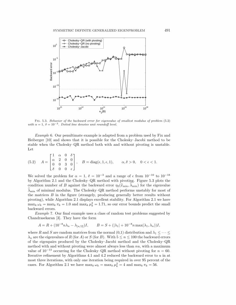
Fig. 5.3. Behavior of the backward error for eigenvalue of smallest modulus of problem (5.2)with α = 1, δ = 10−3. Dotted line denotes unit roundoff level.

Example 6. Our penultimate example is adapted from a problem used by Fix andHeiberger [10] and shows that it is possible for the Cholesky–Jacobi method to bestable when the Cholesky–QR method both with and without pivoting is unstable.Let

A =

1 α 0 δα 2 0 00 0 3 0δ 0 0 ε

, B = diag(ε, 1, ε, 1), α, δ > 0, 0 < ε < 1.(5.2)

We solved the problem for α = 1, δ = 10−3 and a range of ε from 10−10 to 10−18

by Algorithm 2.1 and the Cholesky–QR method with pivoting. Figure 5.3 plots thecondition number of B against the backward error η2(xmin, λmin) for the eigenvalue

λmin of minimal modulus. The Cholesky–QR method performs unstably for most ofthe matrices B in the figure (strangely, producing generally better results withoutpivoting), while Algorithm 2.1 displays excellent stability. For Algorithm 2.1 we havemaxk ωk = maxk πk = 1.0 and maxk µ

2k = 1.71, so our error bounds predict the small

backward errors.Example 7. Our final example uses a class of random test problems suggested by

Chandrasekaran [3]. They have the form

A = R+ (10−8nλn − λ[n/2])I, B = S + (|λ1|+ 10−8nmax(λ1, λn))I,

where R and S are random matrices from the normal (0,1) distribution and λ1 ≤ · · · ≤λn are the eigenvalues of R (for A) or S (for B). With 5 ≤ n ≤ 100 the backward errorsof the eigenpairs produced by the Cholesky–Jacobi method and the Cholesky–QRmethod with and without pivoting were almost always less than nu, with a maximumvalue of 10−13 occurring for the Cholesky–QR method without pivoting for n = 60.Iterative refinement by Algorithms 4.1 and 4.2 reduced the backward error to u in atmost three iterations, with only one iteration being required in over 95 percent of thecases. For Algorithm 2.1 we have maxk ωk = maxk µ

2k = 4 and maxk πk = 56.


6. Conclusions. We have shown that the Cholesky–Jacobi method has betternumerical stability properties than the standard backward error bound (1.7) suggests.For problems with an ill-conditioned B, the method can be, and often is, perfectlystable, and numerical experiments show that our bounds predict the stability well.The method is of practical use: it is easy to code, as Algorithm 2.1 shows, and theJacobi method is particularly attractive in a parallel computing environment.

In practice, the Cholesky–QR method appears to perform as well as the Cholesky–Jacobi method, provided that complete pivoting is used in the Cholesky factorization.As we noted in section 1 this can, to some extent, be explained by the QR method’sgood performance on graded matrices. However, except for a rarely used variantemploying Givens tridiagonalization, the best backward error bound for the Cholesky–QR method continues to contain a factor κ2(B). It is an important open problem toderive a sharper bound.

Instability of the Cholesky methods can be cured by iterative refinement, providedit is not too severe, as we have illustrated. Drawbacks are that refinement is expensiveif applied to more than just a few eigenpairs, and practically verifiable conditions thatguarantee convergence to the desired eigenpair are not available, though the methodis surprisingly effective in practice.

The Cholesky–QR method (without pivoting) is the standard method for solvingthe symmetric definite generalized eigenproblem in LAPACK, MATLAB 6, and theNAG Library, all of which aim to provide exclusively backward stable algorithms. Itis clearly desirable for these implementations to incorporate pivoting in the Choleskyfactorization, in order to enhance the reliability, and to incorporate the option ofiterative refinement of selected eigenpairs, to ameliorate those instances, which arerarer than we can explain, where the Cholesky–QR method behaves unstably.

Acknowledgment. We thank Sven Hammarling for many helpful discussions onthis work.

REFERENCES

[1] E. Anderson, Z. Bai, C. H. Bischof, S. Blackford, J. W. Demmel, J. J. Dongarra, J. J.Du Croz, A. Greenbaum, S. J. Hammarling, A. McKenney, and D. C. Sorensen,LAPACK Users’ Guide, 3rd ed., SIAM, Philadelphia, 1999.

[2] M. F. Anjos, S. J. Hammarling, and C. C. Paige, Solving the Generalized Symmetric Eigen-value Problem, manuscript, 1992.

[3] S. Chandrasekaran, An efficient and stable algorithm for the symmetric-definite generalizedeigenvalue problem, SIAM J. Matrix Anal. Appl., 21 (2000), pp. 1202–1228.

[4] B. N. Datta, Numerical Linear Algebra and Applications, Brooks/Cole, Pacific Grove, CA,1995.

[5] P. I. Davies, Solving the Symmetric Definite Generalized Eigenvalue Problem, Ph.D. thesis,University of Manchester, Manchester, England, 2000.

[6] J. W. Demmel, Applied Numerical Linear Algebra, SIAM, Philadelphia, 1997.[7] J. W. Demmel and K. Veselic, Jacobi’s method is more accurate than QR, SIAM J. Matrix

Anal. Appl., 13 (1992), pp. 1204–1245.[8] J. J. Dongarra, Algorithm 589 SICEDR: A FORTRAN subroutine for improving the accuracy

of computed matrix eigenvalues, ACM Trans. Math. Software, 8 (1982), pp. 371–375.[9] J. J. Dongarra, C. B. Moler, and J. H. Wilkinson, Improving the accuracy of computed

eigenvalues and eigenvectors, SIAM J. Numer. Anal., 20 (1983), pp. 23–45.[10] G. Fix and R. Heiberger, An algorithm for the ill-conditioned generalized eigenvalue problem,

SIAM J. Numer. Anal., 9 (1972), pp. 78–88.[11] V. Fraysse and V. Toumazou, A note on the normwise perturbation theory for the regular

generalized eigenproblem, Numer. Linear Algebra Appl., 5 (1998), pp. 1–10.[12] G. H. Golub and C. F. Van Loan, Matrix Computations, 3rd ed., Johns Hopkins University

Press, Baltimore, MD, 1996.


[13] D. J. Higham and N. J. Higham, Structured backward error and condition of generalizedeigenvalue problems, SIAM J. Matrix Anal. Appl., 20 (1998), pp. 493–512.

[14] N. J. Higham, Accuracy and Stability of Numerical Algorithms, SIAM, Philadelphia, 1996.[15] N. J. Higham, Iterative refinement for linear systems and LAPACK, IMA J. Numer. Anal.,

17 (1997), pp. 495–509.[16] W. Kerner, Large-scale complex eigenvalue problems, J. Comput. Phys., 85 (1989), pp. 1–85.[17] L. Meirovitch, Elements of Vibration Analysis, 2nd ed., McGraw-Hill, New York, 1986.[18] C. B. Moler and G. W. Stewart, An algorithm for generalized matrix eigenvalue problems,

SIAM J. Numer. Anal., 10 (1973), pp. 241–256.[19] B. N. Parlett, The Symmetric Eigenvalue Problem, SIAM, Philadelphia, 1997.[20] G. Peters and J. H. Wilkinson, Ax = λBx and the generalized eigenproblem, SIAM J.

Numer. Anal., 7 (1970), pp. 479–492.[21] G. W. Stewart, Introduction to Matrix Computations, Academic Press, New York, 1973.[22] H. J. Symm and J. H. Wilkinson, Realistic error bounds for a simple eigenvalue and its

associated eigenvector, Numer. Math., 35 (1980), pp. 113–126.[23] F. Tisseur, Newton’s method in floating point arithmetic and iterative refinement of generalized

eigenvalue problems, SIAM J. Matrix Anal. Appl., 22 (2001), pp. 1038–1057.[24] A. van der Sluis, Condition numbers and equilibration of matrices, Numer. Math., 14 (1969),

pp. 14–23.[25] J. H. Wilkinson, The Algebraic Eigenvalue Problem, Oxford University Press, Oxford, UK,

1965.[26] J. H. Wilkinson, Error analysis revisited, Bull. Inst. Math. Appl., 22 (1986), pp. 192–200.

Documents

Analysis of the Cholesky Method with Iterative Reﬁnement ...eprints.ma.man.ac.uk/1123/01/covered/MIMS_ep2008_70.pdf · Analysis of the Cholesky Method with Iterative Reﬁnement