Analysis of supercavitating and surface-piercing propeller flows via BEMY. L. Young, S. A. Kinnas

Abstract A low-order potential based 3-D boundaryelement method (BEM) is presented for the analysis ofunsteady sheet cavitation on supercavitating and surface-piercing propellers. The method has been developed in thepast for the prediction of unsteady sheet cavitation forconventional propellers. To allow for the treatment ofsupercavitating propellers, the method is extended tomodel the separated flow behind trailing edge with non-zero thickness. For surface-piercing propellers, the nega-tive image method is used, which applies the linearizedfree surface boundary condition with the infinite Froudenumber assumption. The method is shown to convergequickly with grid size and time step size. The predictedcavity planforms and propeller loadings also compare wellwith experimental observations and measurements.

Keywords BEM, Cavitation, Super cavitating propeller,Surface-piercing propeller

1IntroductionHydrodynamic cavitation is defined as the formation andcollapse of partial vacuums in a liquid by a swiftly movingsolid body. It can occur in any hydrodynamic devices thatoperate in liquid when pressure drops below the saturatedvapor pressure. In the past, the goal in the design ofhydrodynamic devices was to avoid cavitation because ofits undesirable effects, which include blade surface erosion,

increased hull pressure fluctuation and vibration, acousticenergy radiation, and blade vibration. However, few pro-pellers in practice can operate entirely without cavitationdue to the non-axisymmetric inflow or unsteady bodymotion. Furthermore, propellers without cavitation wouldneed to be larger and slower than necessary.

The objective of this work is to extend a 3-D boundaryelement method, which has been developed in the past forthe prediction of unsteady sheet cavitation on conven-tional fully submerged propellers, to predict the perfor-mance of supercavitating and surface-piercing propellers.

1.1Supercavitating propellersSupercavitating propellers are often believed to be themost fuel efficient propulsive device for high speed vessels.The term supercavity refer to a cavity that is longer thanthe blade. It tends to have smaller volume change andproduce bubbles which collapse downstream of the bladetrailing edge, which results in reduced noise and bladesurface erosion.

The development of numerical methods for the analysisand design of supercavitating propellers has been slowcompared to conventional propellers. The main difficultyarises from the unknown physics in the highly turbulentregion behind blunt trailing edges, which is characteristicof supercavitating propeller sections. The first theoreticaldesign method was developed by (Tachnimdji and Mor-gan, 1958), and followed by (Tulin, 1962; Cox, 1968; Barr,1970; Yim, 1976). However, these methods were based on2-D studies, and required many approximations andempirical corrections. Recently, more rigorous methodswere developed by (Kamirisa and Aoki, 1994; Kikuchiet al., 1994; Vorus and Mitchell, 1994; Ukon et al., 1995).Nevertheless, these methods were still based on the opti-mization of 2-D cavitating blade sections to yield minimaldrag for a given lift and cavitation number.

A 3-D vortex-lattice method was developed by (Kudoand Ukon, 1994) to predict the steady performance ofsupercavitating propellers. Their model assumed thepressure over the separated zone to be constant and equalto the vapor pressure. A variable length separated zonemodel using a similar vortex-lattice method was presentedin (Kudo and Kinnas, 1995).

However, all of the above mentioned lifting surfacemethods cannot capture accurately the flow details at theblade leading and trailing edge due to the breakdown oflinear cavity theory. In addition, the applicability of thethickness-loading coupling introduced by (Kinnas, 1992)

Computational Mechanics 32 (2003) 269–280 � Springer-Verlag 2003

DOI 10.1007/s00466-003-0484-6

269

Y. L. YoungDepartment of Civil and Environmental Engineering,E-326, Princeton University, Princeton, NJ, 08544

This work was completed while as a doctoral student at TheUniversity of Texas at Austin

S. A. Kinnas (&)Ocean Engineering Group, Department of Civil Engineering,C1786, The University of Texas at Austin,1 University Station, Austin, TX 78712E-mail: kinnas@mail.utexas.edu

Support for this research was provided by Phase III of the‘‘Consortium on Cavitation Performance of High SpeedPropulsors’’ with the following members: AB Volvo Penta,American Bureau of Shipping, El Pardo Model Basin, HyundaiMaritime Research Institute, Kamewa AB, Michigan WheelCorporation, Naval Surface Warfare Center Carderock Division,Office of Naval Research (Contract N000140110225), UlsteinPropeller AS, VA Tech Escher Wyss GMBH, and WartsilaPropulsion.

in the analysis of supercavitating propellers is still underinvestigation.

1.2Surface-piercing propellersA surface-piercing (also called partially submerged) pro-peller is a special type of supercavitating propeller whichoperates at partially submerged conditions. Surface-piercing propellers are more efficient than submergedsupercavitating propellers because of (1) the reduction ofappendage drag, and (2) the possibility of larger propellerdiameter.

The first theoretical effort to model partially submergedpropeller was carried out by (Oberembt, 1968) using alifting line approach. He assumed the propeller to belightly loaded such that no natural ventilation of thepropeller and its vortex wake occurs. Later, (Furuya, 1985)also used a lifting-line approach, but he included the effectof propeller ventilation. The method was combined with a2-D water entry-and-exit theory developed by (Wang,1979) to determine thrust and torque coefficients.

An unsteady lifting surface method was employed by(Wang et al., 1990) for the analysis of 3-D fully ventilatedthin foils entering into initially calm water. The methodwas later extended by (Wang et al., 1992) to predict theperformance of fully ventilated partially submerged pro-peller with its shaft above the water surface. Similar to(Furuya, 1985), the negative image method was used toaccount for free surface effect, and the blade was assumedto be fully ventilated on the suction side starting from theblade leading edge. The effect of the blade thickness wasalso neglected in the computation.

The 3-D vortex-lattice lifting surface method developedby (Kudo and Kinnas, 1955) for the analysis of supercav-itating propellers has also been extended for the analysis ofsurface-piercing propellers. However, the method per-forms all the calculations assuming the propeller is fullysubmerged, then multiplies the resulting forces with thepropeller submergence ratio. As a result, only the meanforces can be predicted while the complicated phenomenaof blade’s entry to, and exit from, the water surface arecompletely ignored.

A 2-D time-marching BEM was developed by (Savineauand Kinnas, 1995) for the analysis of the flow field arounda fully ventilated partially submerged hydrofoil. However,this method only accounts for the hydrofoil’s entry to, butnot exit from, the water surface.

1.3A low-order potential based BEMIn the present method, a low-order (piecewise constantdipole and source distributions) potential-based boundaryelement method is used to predict the performance ofsupercavitating and surface-piercing propellers.

The low-order potential based BEM was first applied forthe analysis of marine propeller in steady flow by (Lee,1987; Kerwin et al., 1987) and unsteady flow by (Hsin, 1990;Kinnas and Hsin, 1992). The method was then extended forthe analysis of flow around 2-D partially and supercavi-tating hydrofoils (Kinnas and Fine, 1991) and 3-D partiallycavitating hydrofoils (Fine and Kinnas, 1993a). In (Kinnas

and Fine, 1992), the method was named PROPCAV(PROPeller CAVitation) for its added ability to analyze 3-Dunsteady flow around cavitating propellers. Later, (Mullerand Kinnas, 1999) modified the method to search formidchord cavitation on either the back or the face ofpropeller blades. Most recently, (Young and Kinnas, 2001)extended the method to predict alternating or simultaneousface and back cavitation on conventional propeller bladessubjected to non-axisymmetric inflow. The boundary ele-ment method inherently includes the effect of non-linearthickness-loading coupling by discretizing the blade sur-face instead of the mean camber surface. Thus, it requiresmore central processing unit (CPU) time and memory thanthe lifting surface method. However, it offers a better pre-diction of the flow details at the propeller leading edge andtip than the lifting surface method.

2FormulationThe formulation for supercavitating propellers is similar tothat for conventional cavitating propellers. It is given in(Kinnas and Fine, 1992; Young and kinnas, 2001), and issummarized here for the sake of completeness.

Consider a cavitating propeller subjected to a general

inflow wake ~qqwðxs; ys; zsÞ1, as shown in Fig. 1. The inflowvelocity,~qqin, with respect to the propeller fixed coordinatesðx; y; zÞ, can be expressed as the sum of the inflow wakevelocity, ~qqw, and the propeller’s angular velocity ~xx, at agiven location ~xx:

~qqinðx; y; z; tÞ ¼~qqwðx; r; hB � xtÞ þ ~xx�~xx ð1Þwhere r ¼

ffiffiffiffiffiffiffiffiffiffiffiffiffiffi

y2 þ z2p

, hB ¼ arctanðz=yÞ, and ~xx ¼ ðx; y; zÞ.The resulting flow is assumed to be incompressible andinviscid. Hence, the total velocity, ~qq, can be expressed interms of ~qqin and the perturbation potential /:

~qqðx; y; z; tÞ ¼~qqinðx; y; z; tÞ þ r/ðx; y; z; tÞ ð2Þ

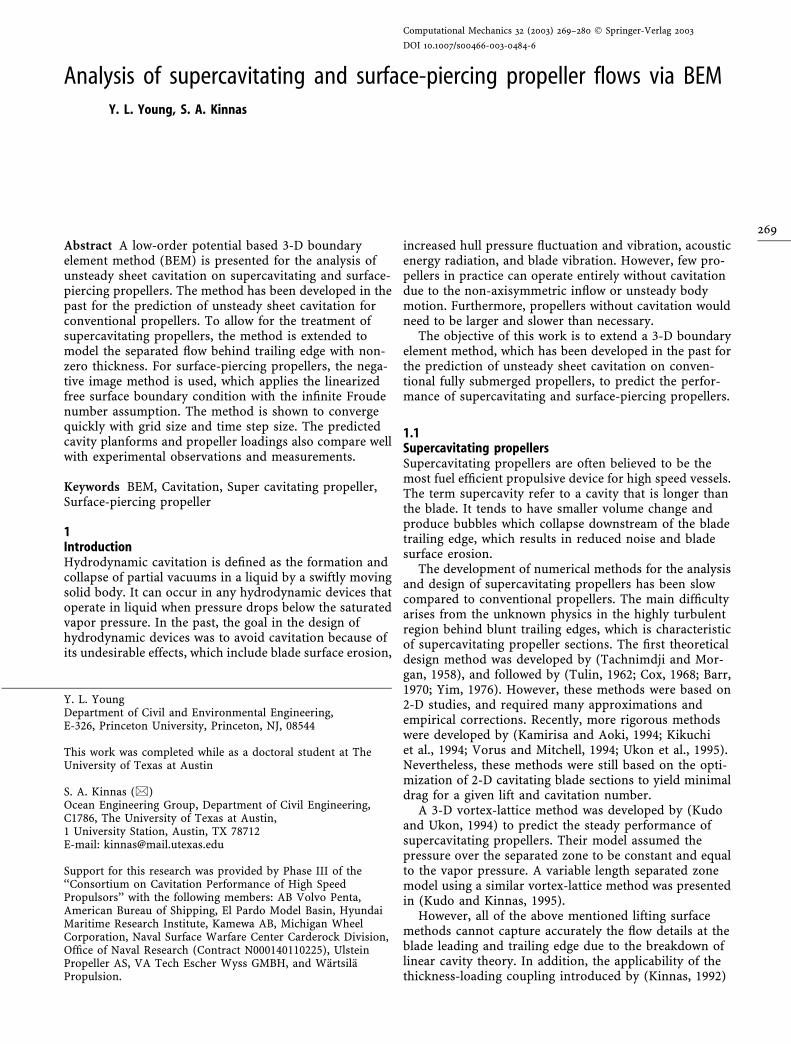
Fig. 1. Propeller subjected to a general inflow wake. The pro-peller fixed ðx; y; zÞ and ship fixed ðxs; ys; zsÞ coordinate systemsare shown. From (Young and Kinnas, 2003)

1 ~qqw is assumed to be the effective wake, i.e. it includes theinteraction between the vorticity in the inflow and the propeller(Kinnas et al., 2000; Choi, 2000).

270

where / satisfies the Laplace’s equation in the fluiddomain (i.e. r2/ ¼ 0). Note that the propeller fixedcoordinates system is used in analyzing the flow.

2.1The boundary integral equationThe perturbation potential, /, at every point p on thecombined wetted blade and cavity surface, SWBðtÞ [ SCðtÞ,must satisfy Green’s third identity:

2p/pðtÞ

¼Z Z

SWBðtÞ[SCðtÞ

/qðtÞoGðp; qÞonqðtÞ

� Gðp; qÞo/qðtÞonqðtÞ

� �

dS

þZ Z

SW ðtÞ

D/ðrq; hq; tÞoGðp; qÞonqðtÞ

dS;

p 2 SWBðtÞ [ SCðtÞ ð3Þwhere the subscript q corresponds to the variable point inthe integration. Gðp; qÞ ¼ 1=Rðp; qÞ is Green’s function inan unbounded 3-D fluid domain, with Rðp; qÞ being thedistance between points p and q. ~nnq is the unit vectornormal to the integration surface, with the positivedirection pointing into the fluid domain. SWBðtÞ denotesthe wetted blade and hub surfaces, and SCðtÞ denotes thecavitating surfaces.

The wake surface, SWðtÞ, is assumed to have zerothickness. The geometry of the wake surface is determinedby satisfying the force-free wake condition, which requireszero pressure jump across the wake sheet. In this work, thewake is aligned with the circumferentially averaged inflowusing a iterative lifting surface method developed by(Greeley and Kerwin, 1982). As stated in (Greeley andKerwin, 1982), this method ‘‘artificially’’ suppresses thewake roll-up. Recently, a fully unsteady wake alignmentmethod, including wake roll-up and developed tip vortexcavity, is developed for propellers in non-axisymmetricinflows (Lee and Kinnas, 2001; Lee and Kinnas, 2002). Theformulation and results using this unsteady wake align-ment method is presented in (Lee and Kinnas, 2001; Leeand Kinnas, 2002; Lee, 2002).

The dipole strength D/ðr; h; tÞ in the wake is convectedalong the assumed wake model with angular speed x:

D/ðr; h; tÞ ¼ D/T rT ; t �h� hT

x

� �

; t � h� hT

x

D/ðr; h; tÞ ¼ D/SðrTÞ; t <h� hT

xð4Þ

where ðr; hÞ are the cylindrical coordinates at any point inthe trailing wake surface (SW ), and ðrT ; hTÞ are trailingedge coordinates of the corresponding streamline. D/S isthe steady flow potential jump in the wake whenthe propeller is subject to the circumferentially averagedflow.

The value of the dipole strength, D/TðrT ; tÞ, at thetrailing edge of the blade at radius rT and time t, is givenby Morino’s Kutta condition (Morino and Kuo, 1974):

D/TðrT; tÞ ¼ /þT ðrT ; tÞ � /�T ðrT ; tÞ ð5Þ

where /þT ðrT ; tÞ and /�T ðrT ; tÞ are the values of thepotential at the upper (suction side) and the lower (pres-sure side) blade trailing edge, respectively, at time t.

Note that Eq. (3) is a Fredholm singular integralequation of the second kind. It should be applied on the‘‘exact’’ cavity surface SC, as shown on the top of Fig. 2.However, the cavity surface is not known and has to bedetermined as part of the solution. In this work, anapproximated cavity surface, shown on the bottom ofFig. 2, is used. The approximated cavity surface is com-prised of the blade surface underneath the cavity on theblade, SCBðtÞ, and the portion of the wake surface which isoverlapped by the cavity, SCWðtÞ. The justification formaking this approximation, as well as a measure of itseffect on the cavity solution can be found in (Kinnas andFine, 1993; Fine, 1992).

Using the approximated cavity surface, Eq. (3) may bedecomposed into a summation of integrals over the bladesurface, SB (� SCB [ SWBÞ, and the portion of the wakesurface which is overlapped by the cavity, SCW .

2.2Boundary conditionsEquation 3 implies that the perturbation potential (/p)can be expressed as: (1) continuous source (G) and dipole(oG=on) distributions on the wetted blade (SWB) and cavity(SCB [ SCW ) surfaces, and (2) continuous dipole distribu-tion on the wake surface SW . Thus, /p can be uniquelydetermined by satisfying the following boundaryconditions:

Kinematic boundary condition on wettedblade and hub surfacesThe kinematic boundary condition requires the flow to betangent to the wetted blade and hub surface, which forms aNeumann-type boundary condition for o/=on:

Fig. 2. Top: Definition of the exact surface. Bottom: Definitionof the approximated cavity surface. From (Young and Kinnas, 2001)

271

o/on¼ �~qqin �~nn ð6Þ

Dynamic boundary condition on cavitating surfacesThe dynamic boundary condition on the cavitating bladeand wake surfaces requires the pressure everywhere on thecavity to be constant and equal to the vapor pressure, Pv.By applying Bernoulli’s equation, the total cavity velocity,~qqc, can be expressed as follows:

~qqc

�

�

�

�

2¼ n2D2rn þ ~qqw

�

�

�

�

2þx2r2 � 2gys � 2o/ot

ð7Þ

where rn � ðPo � PvÞ=ðq2 n2D2Þ is the cavitation number; qis the fluid density and r is the distance from the axis ofrotation. Po is the pressure far upstream on the shaft axis;g is the acceleration of gravity and ys is the ship fixedcoordinate, shown in Fig. 1. n ¼ x=2p and D are thepropeller rotational frequency and diameter, respectively.

The total cavity velocity can also be expressed in termsof the local derivatives along the s (chordwise), v(spanwise), and n (normal) grid directions:

~qqc ¼Vs~ss� ð~ss �~vvÞ~vv½ � þ Vv~vv� ð~ss �~vvÞ~ss½ �

k~ss�~vvk2 þ ðVnÞ~nn ð8Þ

where~ss, ~vv, and ~nn denote the unit vectors along the non-orthogonal curvilinear coordinates s, v, and n, respectively.The total velocities on the local coordinates (Vs;Vv;Vn) aredefined as follows:

Vs �o/osþ~qqin �~ss; Vv �

o/ovþ~qqin �~vv;

Vn �o/onþ~qqin �~nn ð9Þ

Note that if s, v, and n were located on the ‘‘exact’’ cavitysurface, then the total normal velocity, Vn, would be zero.However, this is not the case since the cavity surface isapproximated with the blade surface beneath the cavityand the wake surface overlapped by the cavity. AlthoughVn may not be exactly zero on the approximated cavitysurface, it is small enough to be neglected in the dynamicboundary condition (Fine, 1992).

Equations 7 and 8 can be integrated to form a quadraticequation in terms of the unknown chordwise perturbationvelocity o/=os. By selecting the root which corresponds tothe cavity velocity vectors that point downstream, thefollowing expression can be derived:

o/os¼ �~qqin �~ssþ Vv cos wþ sin w

ffiffiffiffiffiffiffiffiffiffiffiffiffiffiffiffiffiffiffiffi

j~qqcj2 � V2

v

q

ð10Þ

where w is the angle between s and v directions, as shownin Fig. 2. Equation 10 can then integrated to form aDirichlet type boundary condition for /. It should benoted that the terms o/=ot and o/=ov inside j~qqcj and Vv inEq. 10 are also unknown and are determined in aniterative manner.

On the cavitating wake surface, the coordinate s isassumed to follow the streamlines. It was found that thecrossflow term (o=ov) in the cavitating wake region had avery small effect on the solution (Fine, 1992; Fine and

Kinnas, 1993b). Thus, the total cross flow velocity is as-sumed to be small, which renders the following expressionon the cavitating wake surface:

o/os¼ �~qqin �~ssþ j~qqcj ð11Þ

Kinematic boundary condition on cavitating surfacesThe kinematic boundary condition requires that the totalvelocity normal to the cavity surface to be zero:

0 ¼ D

Dtðn� hðs; v; tÞÞ ¼ o

otþ~qqcðx; y; z; tÞ �~rr

� �

� ðn� hðs; v; tÞÞ ð12Þwhere n and h are the curvilinear coordinate and cavitythickness normal to the blade surface, respectively.

Substituting Eq. (8) into Eq. (12) yields the followingpartial differential equation for h on the blade (Kinnas andFine, 1992):

oh

osVs � cos wVv½ � þ oh

ovVv � cos wVs½ �

¼ sin2w Vn �oh

ot

� �

ð13Þ

Assuming again that the spanwise crossflow velocity onthe wake surface is small, the kinematic boundary condi-tion reduces to the following equation for the cavitythickness (hw) in the wake:

o/þ

on� o/�

on

� �

� ohw

ot¼ j~qqcj

ohw

osð14Þ

Note that hw in Eq. 14 is defined normal to the wakesurface. In addition, the quantity hw at the blade trailingedge is determined by interpolating the upper and/orlower cavity surface over the blade and computing itsnormal offset from the wake sheet.

Cavity closure conditionThe extent of the unsteady cavity is unknown and has tobe determined as part of the solution. The cavity length ateach radius r and time t is given by the function lðr; tÞ. Fora given cavitation number, rn, the cavity planform, lðr; tÞ,must satisfy the following condition:

d lðr; tÞ; r; rnð Þ ¼ 0 ð15Þwhere d is the thickness of the cavity trailing edge.Equation 15 requires that the cavity closes at its trailingedge. This requirement is the basis of a Newton-Raphsoniterative method that is used to find the cavity planform(Kinnas and Fine, 1993).

Cavity detachment conditionThe cavity detachment locations are determined iterativelyby satisfying the Villat-Brillouin smooth detachmentcondition (Brillouin, 1911; Villat, 1914). This conditionrequires that the cavities do not intersect the blade at itsleading edge, and the pressure upstream of the cavities tobe greater than the vapor pressure. It should be noted thatthe current work assumes the flow to be inviscid. It is

272

widely known that viscosity affects the cavity detachment,as well as the extent and thickness of the cavity. However,investigations by (Kinnas et al., 1994) concluded that theeffect of viscosity on the predicted cavity extent andvolume is negligible for the case of supercavitation.

2.3Solution algorithmThe unsteady cavity problem is solved by inverting Eq. (3)subject to Eqs. (4), (5), (6), (10), (11), (15), and the cavitydetachment condition. The integral surfaces are approxi-mated with hyperboloidal panels (Kinnas and Hsin, 1992)on which constant strength dipoles and sources are dis-tributed. Eq. (3) is applied at the panel centroids in orderto determine the potentials at each panel. The problem issolved in the time domain with constant time step size Dt.

The numerical implementation is described in detail in(Kinnas and Fine, 1992). In brief, for a given cavity plan-form, Green’s formula is solved with respect to unknown /on the wetted blade and hub surfaces, and unknowno/=on on the cavitating surfaces. The cavity heights on theblade and the wake are computed by differentiatingEqs. (13) and (14) with a second order central finite dif-ference method. The extent of cavities at each time step isobtained iteratively using a Newton-Raphson techniquewhich requires Eq. (15) to be satisfied everywhere on theblade at each time step. Finally, the correct cavity planformis obtained by adjusting the cavity detachment locationsuntil the smooth detachment condition is satisfied. Itshould be noted that the split-panel method developed by(Kinnas and Fine, 1993) is used to treat panels which areintersected by the cavity trailing edge. In addition, at eachtime step, the solution is only obtained for the key blade.The influence of each of the other blades is accounted forin a progressive manner by using the solution from anearlier time step when the key blade was in the position ofthat blade.

3Supercavitating propellersExperimental evidence showed that the separated zonebehind the thick blade trailing edge forms a closed cavity

that separates from the practically ideal irrotational flowaround a supercavitating blade section (Russel, 1958). Inaddition, the pressure within the separated zone (alsocalled the base pressure) can be assumed to be uniform(Riabouchinsky, 1926; Tulin, 1953). However, a turbulentdissipation model (such as the one used in (Vorus andChen, 1987)) is necessary to determine the the mean basepressure and the extent of the separated zone, which is notpractical for engineering purposes.

In the present method, the base pressure is assumed tobe constant and equal to the vapor pressure, similar to thatassumed in (Kudo and Ukon, 1994). Hence, the separatedzone can be solved for like an additional cavitation bubble.To avoid ‘‘openness’’ at the blade trailing edge, a smallinitial closing zone, shown in Fig. 3, is introduced. Theprecise geometry of the initial closing zone is not impor-tant, as long as it is inside the separated region and itstrailing edge lies on the aligned wake sheet. The method ismodified so that it treats the original blade and the initialclosing zone as one solid body. It should be noted that theinitial closing zone is used in the entire analysis, and itsgeometry does not change with time. However, the sizeand the extent of the cavities and the separated regions areallowed to change with time, and are solved for as part ofthe solution.

The solution method is the same as that for fully sub-merged conventional propellers. However, additional care isneeded to ensure the potential to be continuous between thewetted portions of the blade, the cavity surfaces, and theclosing zones. An additional condition which requires thecavities to detach prior to the actual blade trailing edge isalso needed. Furthermore, the pressure acting on the thickblade trailing edge must also be included in the force cal-culation. This is accomplished by multiplying the separatedregion pressure acting normal to the blade trailing edge withthe trailing edge area. Details of the numerical algorithm andnumerical validations of the method are presented in(Young, 2002; Young and Kinnas, 2003).

As depicted in Fig. 3, this scheme is applicable to fullywetted, partially cavitating, and supercavitating conditionsin steady and unsteady flows assuming P ¼ Pv in the

Fig. 3. Treatment of supercavitating blade sections. From (Youngand Kinnas, 2003) Fig. 4. Cavitation patterns on supercavitating propellers that can

be predicted by the present method. From (Young and Kinnas,2003)

273

separated region. Cavitation patterns on supercavitatingpropellers that can be predicted by the present method areshown in Fig. 4.

3.1Numerical validationsIn order to validate the method, parametric studies areconducted for a rectangular hydrofoil at an angle of attacka ¼ 1�. The cross section of the hydrofoil is modified fromthat of a NACA66 thickness distribution with NACA a = 0.8mean camber line. The maximum thickness to chord ratio(Tmax=C) is 0.05. The thickness to chord ratio at the foiltrailing edge (TTE=C) is 0.02. The maximum camber tochord ratio (fmax=C) is 0.02. The predicted cavity planformand cavitating pressure distribution are shown in Fig. 5.Notice that there are midchord supercavitation on the backside of the hydrofoil, and leading edge partial cavitation onthe face side of the hydrofoil. In addition, notice that thesmooth detachment condition and the cavity closurecondition are satisfied everywhere on the hydrofoil.

The influence of the initial closing zone length on thepressure and cavity shape is shown in Fig. 6. Since theentire initial closing zone is inside the separated region,the length of the initial closing zone should have negligibleinfluence on the solution, which is confirmed by Fig. 6.

In order to assess the uniqueness of the solution, thesensitivity of the total cavity volume to the initial guess ofcavity lengths on the suction side (lþi ) and on the pressureside (l�i ) is shown in Fig. 7. The quantity NTSTEP denotesthe step number. Within each step, a maximum of 30iterations are allowed to determine the cavity lengths whichsatisfy Eq. (15) for the given guess of cavity detachmentlocations. At the end of every step, the cavity detachmentlocations are adjusted via the smooth detachment condi-tion. Note that the initial guess of cavity lengths are non-dimensionalized by the local chord length at each radial

strip. As shown in Fig. 7, the converged solution is inde-pendent of the initial guess of cavity lengths.

The dependence of the 3-D cavity planform on thetolerance (dtol) for cavity trailing edge openness [d asdefined in Eq. (15)] is shown in Fig. 8. Note that both dtol

and d are non-dimensionalized by the local chord length ateach radial strip. As shown in Fig. 8, the solution isinsensitive to dtol for dtol � 0:001.

The convergence of the method with number of panelsis shown in Fig. 9. The error shown in Fig. 9 is computedas follows:

err ¼ CNmid � CNM

mid

�

�

�

� ð16Þwhere CN

mid is the circulation at midspan for N number ofpanels on the foil surface. NM is number of panels on thefoil surface for the finest discretization, which is 7200. Asshown in Fig. 9, the convergence rate is approximately 1.4.

3.2Validation with experimentsTo validate the treatment of supercavitating propellers, thepredicted force coefficients are compared with

Fig. 5. 3-D hydrofoil. rv ¼ 0:11, fmax=C ¼ þ0:02, Tmax=C ¼ 0:05,a ¼ þ1�. Uniform inflow

Fig. 6. Dependence on the initial closing zone length. XSR is thelength ratio of the initial closing zone to the chord. rv ¼ 0:11,fmax=C ¼ þ 0:02, Tmax=C ¼ 0:05, a ¼ þ1�. Uniform inflow

Fig. 7. Dependence on the initial guess of cavity lengths onthe suction side (lþi ) and pressure side (l�i ). rv ¼ 0:11,fmax=C ¼ þ 0:02, Tmax=C ¼ 0:05, a ¼ þ1�. Uniform inflow

274

experimental measurements (Matsuda et al., 1994) for asupercavitating propeller. The test geometry is M.P.No.345(SRI), which is designed using SSPA charts under thefollowing conditions: JA ¼ VA=nD ¼ 1:10,rv ¼ Po � Pv=0:5qV2

A ¼ 0:40, and KT ¼ T=qn2D4 ¼ 0:160.VA is the propeller advance speed. T and Q are the pro-

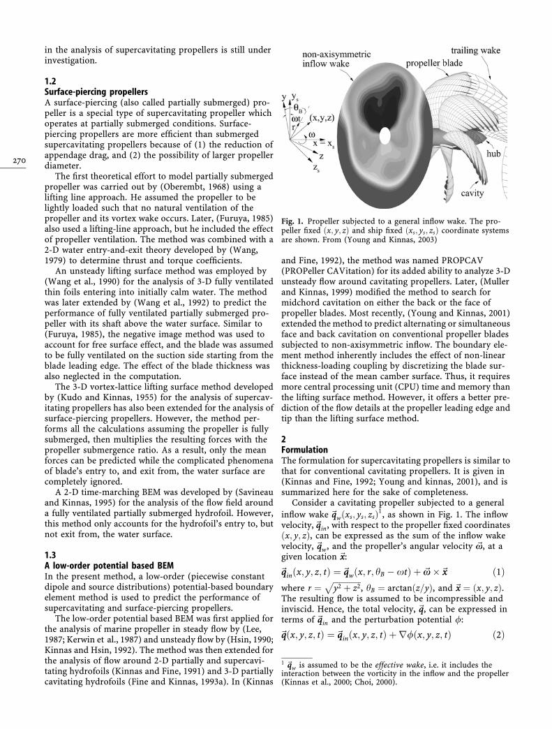
peller thrust and torque. The discretized propeller geom-etry is shown in Fig. 10. Comparisons of the predicted andmeasured thrust (KT), torque (KQ ¼ Q=qn2D5), and effi-ciency ½go ¼ ðKT=KQÞ � ðJA=2pÞ� are shown in Fig. 11. Notethat the ‘‘kink’’ at JA ¼ 1:2 in Fig. 11 is due to the shiftfrom leading edge supercavitation to midchord superca-vitation, as depicted in Fig. 10. It is worth noting that thesmooth detachment condition is satisfied for all JA’s. Inaddition, the method converged quickly with number ofpanels, as demonstrated in Fig. 12. The error, ERR, inFig. 12 is defined with respect to the non-dimensionalcirculation at r=R ¼ 0:7, C0:7, for the finest discretization:

ERR ¼ CN0:7 � CNM

0:7

�

�

�

� ð17Þwhere N is the number of panels on the blade surface. NMis number of panels on the blade surface for the finestdiscretization, which is 5600. It should be noted that

Fig. 8. Dependence on thetolerance for openness at cavitytrailing edge (dtol). rv ¼ 0:11,fmax=C ¼ þ 0:02,Tmax=C ¼ 0:05, a ¼ þ1�.Uniform inflow

Fig. 9. The rate of convergence with respect to number of panelson the foil surface (N). rv ¼ 0:11, fmax=C ¼ þ 0:02,Tmax=C ¼ 0:05, a ¼ þ1�. Uniform inflow

Fig. 10. Discretized geometry of propeller SRI and predictedcavity planform for JA ¼ 1:2 and 1.3

Fig. 11. Comparison of the predicted and versus measured KT ,KQ, and go

275

extensive parametric studies of the method were alsoperformed for this propeller, and are presented in (Youngand Kinnas, 2003).

4Surface-piercing propellersSince surface-piercing propellers are partially submerged,the computational boundary in Eq. (3) must also includethe free surface. As a first step to model partially sub-merged propellers in 3-D, the linearized free surfaceboundary condition is applied to account for the effect ofthe free surface:

o2/ot2ðx; y; z; tÞ þ g

o/oysðx; y; z; tÞ ¼ 0

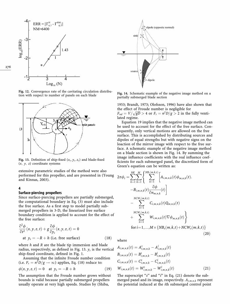
at ys ¼ �Rþ h (i.e. free surface) ð18Þwhere h and R are the blade tip immersion and bladeradius, respectively, as defined in Fig. 13. ys is the verticalship-fixed coordinate, defined in Fig. 1.

Assuming that the infinite Froude number condition(i.e. Fr ¼ n2D=g !1) applies, Eq. (18) reduce to:

/ðx; y; z; tÞ ¼ 0 at ys ¼ �Rþ h ð19ÞThe assumption that the Froude number grows withoutbounds is valid because partially submerged propellersusually operate at very high speeds. Studies by (Shiba,

1953; Brandt, 1973; Olofsson, 1996) have also shown thatthe effect of Froude number is negligible forFnd ¼ V=

ffiffiffiffiffiffi

gDp

> 4 or Fr ¼ n2D=g > 2 in the fully venti-lated regime.

Equation 19 implies that the negative image method canbe used to account for the effect of the free surface. Con-sequently, only vertical motions are allowed on the freesurface. This is accomplished by distributing sources anddipoles of equal strengths but with negative signs on theloaction of the mirror image with respect to the free sur-face. A schematic example of the negative image methodon a blade section is shown in Fig. 14. By summing theimage influence coefficients with the real influence coef-ficients for each submerged panel, the discretized form ofGreen’s equation can be written as:

2p/i ¼X

NK

k¼1

X

M

k¼1

X

NBsðm;k;tÞ

n¼1

�

Ai;m;n;kðtÞ/m;n;kðtÞ(

:

�Bi;m;n;kðtÞo/

onm;n;kðtÞ�

�X

NCWsðm;k;tÞ

n¼1

Ci;m;n;kðtÞQm;n;kðtÞ

þX

NCWsðm;k;tÞ

n¼1

Wi;m;n;kðtÞr/m;n;kðtÞ)

for i¼1;...;M�fNBsðm;k;tÞþNCWsðm;k;tÞgð20Þ

where

Ai;m;n;kðtÞ ¼ Asi;m;n;k � Ai

i;m;n;kðtÞBi;m;n;kðtÞ ¼ Bs

i;m;n;k � Bii;m;n;kðtÞ

Ci;m;n;kðtÞ ¼ Csi;m;n;k � Ci

i;m;n;kðtÞWi;m;n;kðtÞ ¼ Ws

i;m;n;k �Wii;m;n;kðtÞ ð21Þ

The superscript ‘‘s’’ and ‘‘i’’ in Eq. (21) denote the sub-merged panel and its image, respectively. Ai;m;n;k representthe potential induced at the ith submerged control point

Fig. 12. Convergence rate of the cavitating circulation distribu-tion with respect to number of panels on each blade

Fig. 13. Definition of ship-fixed (xs; ys; zs) and blade-fixed(x; y; z) coordinate systems

Fig. 14. Schematic example of the negative image method on apartially submerged blade section

276

on the key blade by unit strength diploes at the real andimaged nth panel on the mth strip of the kth blade. Notethat k ¼ 1 refers to the key blade. Similarly, Bi;m;n;k;Ci;m;n;k,and Wi;m;n;k represent the sum of the real and imageinfluence coefficients due to unit strength source on theblade, unit strength source on the cavitating wake, andunit strength dipole on the wake, respectively. Qm;n;k rep-resents the cavity source strength on the nth panel of themth strip of the kth blade.

Note that the sign in front to the image coefficients in Eq.(21) are negative due to the equal and opposite strengths ofthe image singularities compared to the real singularities. Inaddition, since the problem is solved with respect to thepropeller fixed coordinates which rotates with the key blade,the location of the nth image on the mth strip of the kth bladechanges with time t. The quantities NBs;NCEs, and NWs

represent the number of submerged panels on the blade,cavitating wake, and wake surface, respectively, on the mthstrip of the kth blade. The quantity NK in Eq. (20) representsthe total number blades, while M represents the total num-ber of radial strips per blade.

4.1Solution algorithmFor surface-piercing propellers, Green’s formula is onlysolved for the total number of sub-merged panels on thekey blade and the cavitating portion of the key wake. Thevalues of / and o/=onð Þ are set equal to zero on the bladeand wake panels that are above the free surface. Note thatthe current algorithm does not re-panel the blades andwakes at very time step in order to maintain computationefficiency. As a result, there are some panels that arepartially cut by the free surface. In the present algorithm,the strengths of the singularities are also set equal to zerofor the partially submerged panels. Nevertheless, a methodsimilar to the split-panel technique (Kinnas and Fine,1993) can be applied to account for the effects of thesepanels.

The solution algorithm for partially submerged pro-pellers is similar to that explained earlier for fully sub-merged supercavitating propellers. However, iterations todetermine the correct cavity lengths are no longer neces-sary since the ventilated cavities are assumed to vent to theatmosphere, as observed in experiments.

Ventilated cavity detachment search algorithmDepending on the flow conditions and the blade sectiongeometry, ventilated cavities may detach aft of the bladeleading edge. Thus, the cavity detachment locations on thesuction side of the blade are searched for iteratively at eachtime step until the smooth detachment condition is satis-fied. In addition, due to the interruption of the free sur-face, the following detachment conditions must also besatisfied for partially submerged propellers:

� The ventilated cavities must detach at or prior to theblade trailing edge; and

� During the exit phase (i.e. when part of the blade isdeparting the free surface), the ventilated cavities mustdetach at or aft of the intersection between the bladesection and the free surface.

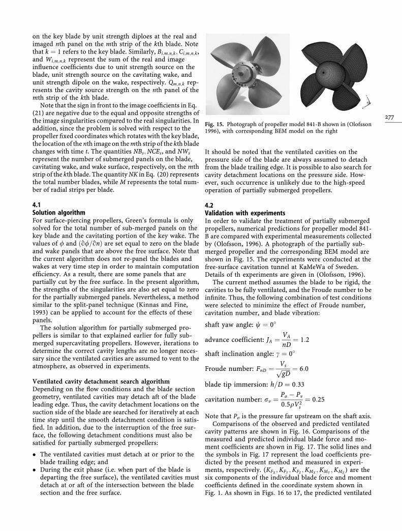
It should be noted that the ventilated cavities on thepressure side of the blade are always assumed to detachfrom the blade trailing edge. It is possible to also search forcavity detachment locations on the pressure side. How-ever, such occurrence is unlikely due to the high-speedoperation of partially submerged propellers.

4.2Validation with experimentsIn order to validate the treatment of partially submergedpropellers, numerical predictions for propeller model 841-B are compared with experimental measurements collectedby (Olofsson, 1996). A photograph of the partially sub-merged propeller and the corresponding BEM model areshown in Fig. 15. The experiments were conducted at thefree-surface cavitation tunnel at KaMeWa of Sweden.Details of th experiments are given in (Olofsson, 1996).

The current method assumes the blade to be rigid, thecavities to be fully ventilated, and the Froude number to beinfinite. Thus, the following combination of test conditionswere selected to minimize the effect of Froude number,cavitation number, and blade vibration:

shaft yaw angle: w ¼ 0�

advance coefficient: JA ¼VA

nD¼ 1:2

shaft inclination angle: c ¼ 0�

Froude number: FnD ¼Vsffiffiffiffiffiffi

gDp ¼ 6:0

blade tip immersion: h=D ¼ 0:33

cavitation number: rv ¼Po � Pv

0:5qV2s

¼ 0:25

Note that Po is the pressure far upstream on the shaft axis.Comparisons of the observed and predicted ventilated

cavity patterns are shown in Fig. 16. Comparisons of themeasured and predicted individual blade force and mo-ment coefficients are shown in Fig. 17. The solid lines andthe symbols in Fig. 17 represent the load coefficients pre-dicted by the present method and measured in experi-ments, respectively. (KFX ;KFY ;KFZ ;KMX ;KMY ;KMZ ) are thesix components of the individual blade force and momentcoefficients defined in the coordinate system shown inFig. 1. As shown in Figs. 16 to 17, the predicted ventilated

Fig. 15. Photograph of propeller model 841-B shown in (Olofsson1996), with corresponding BEM model on the right

277

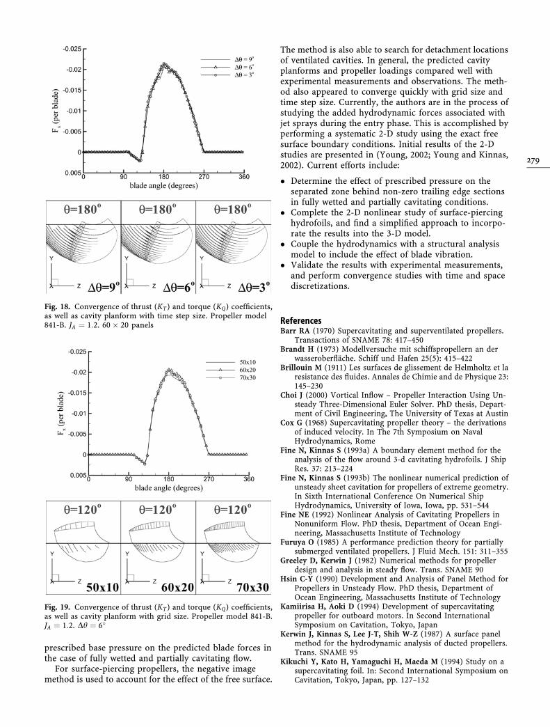
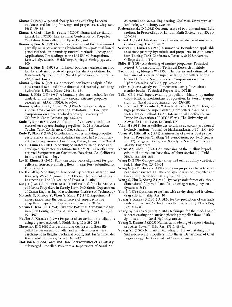
cavity patterns and per blade force agree well withexperiments. In addition, the method also convergedquickly with time step size and grid size, as shown inFigs. 18 and 19.

5ConclusionsA 3-D boundary element method has been extended topredict complex types of cavitation patterns on the backand the face of supercavitating propellers in steady andunsteady flow. The current algorithm assumes the pressureto be constant and equal to the vapor pressure on theseparated region behind non-zero thickness blade trailingedge. Based on this assumption, the method is able topredict the extent and thickness of the separated region.The numerical predictions compared well with experi-mental measurements for steady inflow. The solution alsoconverged with number of panels. Numerical validationstudies using a 3-D hydrofoil seemed very reasonable. Inthe case of supercavitation, the initial closing zone lengthhas no effect on the solution as long as it is inside thesupercavity bubble. The method was also shown to beindependent of the initial guess of cavity lengths and tol-erance of cavity trailing edge openness for dtol � 0:001.The convergence rate for the case of 3-D hydrofoilappeared to be slightly better than linear. However,additional studies are needed to determine the effect of

Fig. 16. Comparison of the observed (top) and predicted (bot-tom) ventilated cavity patterns for JA ¼ 1:2. Propeller model 841-B. 4 Blades. h=D ¼ 0:33. 60 � 20 panels. Dh ¼ 6�. From (Youngand Kinnas, 2002)

Fig. 17. Comparison of predicted (P)and measured (E) blade forces forJA ¼ 1:2. Propeller model 841-B. 4Blades. h=D ¼ 0:33. 60� 20 panels.Dh ¼ 6�. From (Young and Kinnas,2002)

278

prescribed base pressure on the predicted blade forces inthe case of fully wetted and partially cavitating flow.

For surface-piercing propellers, the negative imagemethod is used to account for the effect of the free surface.

The method is also able to search for detachment locationsof ventilated cavities. In general, the predicted cavityplanforms and propeller loadings compared well withexperimental measurements and observations. The meth-od also appeared to converge quickly with grid size andtime step size. Currently, the authors are in the process ofstudying the added hydrodynamic forces associated withjet sprays during the entry phase. This is accomplished byperforming a systematic 2-D study using the exact freesurface boundary conditions. Initial results of the 2-Dstudies are presented in (Young, 2002; Young and Kinnas,2002). Current efforts include:

� Determine the effect of prescribed pressure on theseparated zone behind non-zero trailing edge sectionsin fully wetted and partially cavitating conditions.

� Complete the 2-D nonlinear study of surface-piercinghydrofoils, and find a simplified approach to incorpo-rate the results into the 3-D model.

� Couple the hydrodynamics with a structural analysismodel to include the effect of blade vibration.

� Validate the results with experimental measurements,and perform convergence studies with time and spacediscretizations.

ReferencesBarr RA (1970) Supercavitating and superventilated propellers.

Transactions of SNAME 78: 417–450Brandt H (1973) Modellversuche mit schiffspropellern an der

wasseroberflache. Schiff und Hafen 25(5): 415–422Brillouin M (1911) Les surfaces de glissement de Helmholtz et la

resistance des fluides. Annales de Chimie and de Physique 23:145–230

Choi J (2000) Vortical Inflow – Propeller Interaction Using Un-steady Three-Dimensional Euler Solver. PhD thesis, Depart-ment of Civil Engineering, The University of Texas at Austin

Cox G (1968) Supercavitating propeller theory – the derivationsof induced velocity. In The 7th Symposium on NavalHydrodynamics, Rome

Fine N, Kinnas S (1993a) A boundary element method for theanalysis of the flow around 3-d cavitating hydrofoils. J ShipRes. 37: 213–224

Fine N, Kinnas S (1993b) The nonlinear numerical prediction ofunsteady sheet cavitation for propellers of extreme geometry.In Sixth International Conference On Numerical ShipHydrodynamics, University of Iowa, Iowa, pp. 531–544

Fine NE (1992) Nonlinear Analysis of Cavitating Propellers inNonuniform Flow. PhD thesis, Department of Ocean Engi-neering, Massachusetts Institute of Technology

Furuya O (1985) A performance prediction theory for partiallysubmerged ventilated propellers. J Fluid Mech. 151: 311–355

Greeley D, Kerwin J (1982) Numerical methods for propellerdesign and analysis in steady flow. Trans. SNAME 90

Hsin C-Y (1990) Development and Analysis of Panel Method forPropellers in Unsteady Flow. PhD thesis, Department ofOcean Engineering, Massachusetts Institute of Technology

Kamiirisa H, Aoki D (1994) Development of supercavitatingpropeller for outboard motors. In Second InternationalSymposium on Cavitation, Tokyo, Japan

Kerwin J, Kinnas S, Lee J-T, Shih W-Z (1987) A surface panelmethod for the hydrodynamic analysis of ducted propellers.Trans. SNAME 95

Kikuchi Y, Kato H, Yamaguchi H, Maeda M (1994) Study on asupercavitating foil. In: Second International Symposium onCavitation, Tokyo, Japan, pp. 127–132

Fig. 18. Convergence of thrust (KT) and torque (KQ) coefficients,as well as cavity planform with time step size. Propeller model841-B. JA ¼ 1:2. 60� 20 panels

Fig. 19. Convergence of thrust (KT) and torque (KQ) coefficients,as well as cavity planform with grid size. Propeller model 841-B.JA ¼ 1:2. Dh ¼ 6�

279

Kinnas S (1992) A general theory for the coupling betweenthickness and loading for wings and propellers. J. Ship Res.36(1): 59–68

Kinnas S, Choi J, Lee H, Young J (2000) Numerical cavitationtunnel. In: NCT50, International Conference on PropellerCavitation, Newcastle upon Tyne, England

Kinnas S, Fine N (1991) Non-linear analysis of the flow aroundpartially or super-cavitating hydrofoils by a potential basedpanel method. In: Boundary Integral Methods. Theory andApplications, Proceedings of the IABEM-90 Symposium,Rome, Italy, October Heidelberg. Springer-Verlag, pp. 289–300

Kinnas S, Fine N (1992) A nonlinear boundary element methodfor the analysis of unsteady propeller sheet cavitation. In:Nineteenth Symposium on Naval Hydrodynamics, pp. 717–737, Seoul, Korea

Kinnas S, Fine N (1993) A numerical nonlinear analysis of theflow around two- and three-dimensional partially cavitatinghydrofoils. J. Fluid Mech. 254: 151–181

Kinnas S, Hsin C-Y (1992) A boundary element method for theanalysis of the unsteady flow around extreme propellergeometries. AIAA J. 30(3): 688–696

Kinnas S, Mishima S, Brewer W (1994) Nonlinear analysis ofviscous flow around cavitating hydrofoils. In: TwentiethSymposium on Naval Hydrodynamics, University ofCalifornia, Santa Barbara, pp. 446–465

Kudo T, Kinnas S (1995) Application of vortex/source latticemethod on supercavitating propellers. In 24th AmericanTowing Tank Conference, College Station, TX

Kudo T, Ukon Y (1994) Calculation of supercavitating propellerperformance using a vortex-lattice method. In Second Inter-national Symposium on Cavitation, Tokyo, Japan, pp. 403–408

Lee H, Kinnas S (2001) Modeling of unsteady blade sheet anddeveloped tip vortex cavitation. In: CAV 2001: Fourth Inter-national Symposium on Cavitation, Pasadena, CA. CaliforniaInstitute of Technology

Lee H, Kinnas S (2002) Fully unsteady wake alignment for pro-pellers in non-axisymmetric flows. J. Ship Res (Submitted forPublication)

Lee HS (2002) Modeling of Developed Tip Vortex Cavitation andUnsteady Wake Alignment. PhD thesis, Department of CivilEngineering, The University of Texas at Austin

Lee J-T (1987) A Potential Based Panel Method for The Analysisof Marine Propellers in Steady Flow. PhD thesis, Departmentof Ocean Engineering, Massachusetts Institute of Technology

Matsuda N, Kurobe Y, Ukon Y, Kudo T (1994) Experimentalinvestigation into the performance of supercavitatingpropellers. Papers of Ship Research Institute 31(5)

Morino L, Kuo C-C (1974) Subsonic Potential Aerodynamic forComplex Configurations: A General Theory. AIAA J. 12(2):191–197

Mueller A, Kinnas S (1999) Propeller sheet cavitation predictionsusing a panel method. J. Fluids Eng. 121: 282–288

Oberembt H (1968) Zur bestimmung der instationaren flu-gelkrafte bei einem propeller mit aus dem wasser hera-usschlagenden flugeln. Technical report, Inst. fur Schiffau derUniversitat Hamburg, Bericht Nr. 247

Olofsson N (1996) Force and Flow Characteristics of a PartiallySubmerged Propeller. PhD thesis, Department of Naval Ar-

chitecture and Ocean Engineering, Chalmers University ofTechnology, Goteborg, Sweden

Riabouchinsky D (1962) On some cases of two-dimensional fluidmotion. In Proceedings of London Math Society, Vol. 25, pp.185–194

Russel A (1958) Aerodynamics of wakes, existence of unsteadycavities. Eng. 186: 701–702

Savineau C, Kinnas S (1995) A numerical formulation applicableto surface piercing hydrofoils and propellers. In 24th Amer-ican Towing Tank Conference, Texas A & M University,College Station, TX

Shiba H (1953) Air-drawing of marine propellers. TechnicalReport 9, Transportation Technical Research Institute

Tachnimdji A, Morgan W (1958) The design and estimated per-formance of a series of supercavitating propellers. In theSecond Office of Naval Research Symposium on NavalHydrodynamics, ACR-38, pp. 489–532

Tulin M (1953) Steady two-dimensional cavity flows aboutslender bodies. Technical Report 834, DTMB

Tulin MB (1962) Supercavitating propellers – history, operatingcharacteristics, mechanisms of operation. In Fourth Sympo-sium on Naval Hydrodynamics, pp. 239–286

Ukon Y, Kudo T, Kurobe Y, Matsuda N, Kato H (1995) Design ofhigh performance supercavitating propellers based on avortex lattice method. In An International Conference onPropeller Cavitation (PROPCAV’ 95), The University ofNewcastle Upon Tyne, England, UK

Villat H (1914) Sur la validite des solutions de certain problem d’hydrodynamique. Journal de Mathematiques 6(10): 231–290

Vorus W, Mitchell K (1994) Engineering of power boat propel-lers. In Propellers/Shafting ’94 Symposium, pp. 1–16 (paperNo. 12), Virginia Beach, VA. Society of Naval Architects &Marine Engineers

Vorus WS, Chen L (1987) An extension of the ‘malkus hypoth-esis’ to the turbulent base flow of blunt sections. J. FluidMech. 184: 551–569

Wang D (1979) Oblique water entry and exit of a fully ventilatedfoil. J. Ship Res. 23: 43–54

Wang G, Jia D, Sheng Z (1992) Study on propeller characteristicsnear water surface. In: The 2nd Symposium on Propeller andCavitation, Hangzhon, China, pp. 161–168

Wang G, Zhu X, Sheng Z (1990) Hydrodynamic forces of a three-dimensional fully ventilated foil entering water. J. Hydro-dynamics 5(2):

Yim B (1976) Optimum propellers with cavity-drag and frictionaldrag effects. J. Ship Res. 20

Young Y, Kinnas S (2001) A BEM for the prediction of unsteadymidchord face and/or back propeller cavitation. J. Fluids Eng.123: 311–319

Young Y, Kinnas S (2002) A BEM technique for the modeling ofsupercavitating and surface-piercing propeller flows. 24thSymposium on Naval Hydrodynamics

Young Y, Kinnas S (2003) Numerical modeling of supercavitatingpropeller flows. J. Ship Res. 47(1): 48–62

Young YL (2002) Numerical Modeling of Supercavitating andSurface-Piercing Propellers. PhD thesis, Department of CivilEngineering, The University of Texas at Austin

280