ANALYSIS OF SEVERE ELEVATED THUNDERSTORMS USING …weather.missouri.edu/PRECIP/Thesis-Grempler-DCIN.pdfANALYSIS OF SEVERE ELEVATED THUNDERSTORMS USING DCIN AND DCAPE A Thesis Presented

ANALYSIS OF SEVERE ELEVATED THUNDERSTORMS USING

DCIN AND DCAPE

A Thesis Presented to the Faculty of the Graduate School at the University of Missouri

In Partial Fulfillment of the Requirements for the Degree

Master of Science

by

KEVIN R. GREMPLER

Dr. Patrick Market, Thesis Advisor

MAY 2018

The undersigned, appointed by the dean of the Graduate School, have examined the

thesis entitled

ANALYSIS OF SEVERE ELEVATED CONVECTION OF THE CENTRAL UNITED

STATES

presented by Kevin R. Grempler,

a candidate for the degree of master of science,

and hereby certify that, in their opinion, it is worthy of acceptance.

________________________________________________

Professor Patrick Market

________________________________________________

Professor Neil Fox

________________________________________________

Professor Allen Thompson

ii

ACKNOWLEDGEMENTS

First and foremost, I would like to thank my advisor and committee chair, Dr.

Patrick Market. He has my most sincere gratitude for his guidance and support in

completing this study. Also, I would also like to thank my other committee members, Dr.

Neil Fox and Dr. Allen Thompson for taking time to appraise my performance in this

study. I would like to acknowledge the University of Missouri-Columbia for funding and

for making this research possible. I also would like to thank my family and friends for

their support throughout my graduate years. Lastly, a special thank you goes to my

parents who have always listened and offered me guidance throughout the process.

iii

TABLE OF CONTENTS

ACKNOWLEDGEMENTS ................................................................................................. ii

LIST OF FIGURES ..............................................................................................................v

LIST OF TABLES ............................................................................................................... ix

ABSTRACT ..........................................................................................................................x

CHAPTER 1. INTRODUCTION .........................................................................................1

1.1 Objectives ................................................................................................3

CHAPTER 2. LITERATURE REVIEW ..............................................................................4

2.1 Definitions................................................................................................4

2.2 Occurrences and Frequencies of Elevated Convection ............................5

2.3 Thermodynamic Environment of Elevated Convection ..........................7

2.4 Elevated Convection: Synoptic Conditions .............................................8

2.5 Initiation of Elevated Convection ...........................................................12

2.6 Elevated Convection Associated with Severe Weather Criteria .............14

2.6.1 Climatology of Severe Elevated Thunderstorms .......15

2.6.2 Environment of Elevated Convection with Severe

Winds .........................................................................18

2.6.3 Elevated Convection using DCAPE and DCIN .........19

CHAPTER 3. DATA AND METHODOLOGY .................................................................22

iv

3.1 Data Sources ...........................................................................................22

3.1.1 NCEI, SPC, and WPC ................................................22

3.1.2 RAP and RUC ............................................................23

3.2 Case Selection Criteria ............................................................................25

3.3 Downdraft Penetration of a Stable Layer................................................27

3.3.1 Calculating DCAPE/DCIN .................................................28

CHAPTER 4. RESULTS .....................................................................................................31

4.1 A 10-Year Study ......................................................................................31

4.2 Aggregate Results (Statistical Analysis) .................................................33

4.3 Case Studies ............................................................................................39

4.3.1 Case 1: Iowa, 29 May 2011 .......................................40

4.3.2 Case 2: Kansas/Nebraska/Iowa, 09 Iowa 2013 ..........46

4.3.3 Case 3: Kansas/Nebraska, 13 July 2009 ....................52

4.3.4 Case 4: Michigan, 10 April 2011 ...............................56

CHAPTER 5. Conclusion ....................................................................................................62

5.1 Conclusions ...............................................................................................62

5.2 Future Work ..............................................................................................63

APPENDIX A ......................................................................................................................65

REFERENCES ....................................................................................................................84

v

LIST OF FIGURES

Figure 2.1. Schematic diagrams that summarize the typical conditions associated with

warm-season elevated thunderstorms attended by heavy rainfall: (a) low-level

plan view and (b) middle-upper-level plan view. In (a), dashed lines are

representative 𝜃𝑒values decreasing to the north, dashed-cross lines represent

925-850-hPa moisture convergence maxima, the shaded area is a region of

maximum 𝜃𝑒 advection, the broad stippled arrow denotes the LLJ, the

encircled X represents the MCS centroid location, and the front is indicated

using standard notation. In (b), dashed lines are isotachs associated with the

upper-level jet, solid lines are representative height lines at 500 hPa, the

stippled arrow denotes the 700-hPa jet, and the shaded area indicates where

the mean surface-to-500-hPa relative humidity exceeds 70%. Reproduced

from Moore et al. (2003).. ..................................................................................11

Figure 2.2. Schematic cross-sectional view taken parallel to the LLJ across the frontal

zone. Dashed lines represent typical 𝜃𝑒 values, the larger stippled arrow

represents the ascending LLJ, the thin dotted oval represents the ageostrophic

direct thermal circulation associated with the upper-level jet streak, and the

thick dashed oval represents the direct thermal circulation associated with the

low-level frontogenetical forcing. The area aloft enclosed by dotted lines

indicates upper-level divergence; the area aloft enclosed by solid lines denotes

location of upper-level jet streak. Note that in this cross section the horizontal

distance between the MCS and the location of the upper-level jet maximum is

not to scale. Reproduced from Moore et al. (2003). ..........................................13

Figure 2.3. The number of elevated thunderstorms (reports/station) identified over the 4-

year period (a) from September 1978 through August 1982. Reproduced from

Colman (1990a). ................................................................................................17

Figure 2.4. Total number of elevated severe storm cases by state across the contiguous

United States from the Front Range of the Rocky Mountains eastward to the

Atlantic coast for 1983-87. The black line along the Front Range of the Rocky

Mountains represents the approximate western edge of the domain. Events

that occurred in more than one state were counted multiple times, once for

each state. Reproduced from Horgan et al. (2007). ..........................................18

Figure 3.1. Part of a sounding near the tropopause in a z, T thermodynamic diagram. The

ambient temperature 𝑇𝑎 (heavy uneven line) is approximately constant in the

stratosphere. The lifted temperature 𝑇𝑙 (dashed) is for a parcel from the lower

troposphere. The parcel reaches the peak level when it expands all kinetic

energy. Reproduced from Djuric (1994). ...........................................................28

vi

Figure 4.1. The cases first report of elevated severe thunderstorm: a) All cases (March,

2004-November, 2013), b)Spring (March, April, and May), c) Summer (June,

July, and August), d) Fall (September, October, and December) ......................32

Figure 4.2. Significantly severe (≥5 severe reports) compared to marginally severe (<5

severe reports) thermodynamic variables of elevated thunderstorms Box-and-

Whisker Plot.......................................................................................................34

Figure 4.3. Scatter plot of Marginal cases (black-dots) and Significant cases (green-

squares) are shown to represent similarities between thunderstorms MUCAPE

and DCAPE values measured in J/kg. Black-dotted line represents a 1:1 ratio

of MUCAPE to DCAPE for reference. ..............................................................35

Figure 4.4. Box-and-Whisker plots between all hail and wind dominated cases. ...............36

Figure 4.5. Histograms of DCIN/DCAPE ratio based on initial report of severe weather:

a) Significant cases, b) Marginal cases, c) Hail cases, d) Wind cases. ..............38

Figure 4.6. First reports location for each case with the dominate type of severe weather

represented by blue-dot (hail) and red-star (wind). . .........................................40

Figure 4.7. Severe storm reports on 29 May 2011 from 1121 UTC to 1724 UTC. Red

circle represents the first severe report recorded and the location of sounding

(Fig. 4.10). Reports were acquired from the NCEI. ...........................................41

Figure 4.8. 2-km resolution Base Reflectivity on 29 May 2011 at 1200 UTC. Reproduced

from the Storm Prediction Center. .....................................................................42

Figure 4.9. On 29 May 2011 at 1200 UTC: a) 300-hPa isotachs, streamlines, and

divergence, b)500- hPa observations, heights, and temperatures, c) 850- hPa

observations, heights (black-solid lines), temperatures (red-dotted lines), and

moisture (green), d) Surface analysis. Reproduced from the Storm Prediction

Center and Weather Prediction Center. ............................................................44

Figure 4.10. RAOB sounding analysis for Madison, Iowa on 29 May 2011 at 1100 UTC.

Location represented as red-circle on Figure 4.7. ..............................................45

Figure 4.11. 29 May 2011 at 1100 UTC 2-D display of DCIN (black-solid lines) and

DCAPE (red-dotted lines) with the addition of DCAPE/DCIN ratio equal to 1

and 2 represented in green dotted lines Blue ellipse is representative of where

majority of hail reports occurred. Red ellipse is representative of where

majority of wind reports occurred......................................................................46

Figure 4.12 Severe storm reports on 09-10 April 2013 from 2300 UTC (04/09/2013) to

0345 UTC (04/10/2013). Red circle represents the first severe report recorded

and the location of sounding (Fig. 4.15). Reports were acquired from the

NCEI. .................................................................................................................47

vii

Figure 4.13. 2-km resolution base reflectivity radar mosaic on 10 April 2013 at 0310

UTC. Reproduced from the Storm Prediction Center.. ......................................48

Figure 4.14. On 10 April 2013 at 0000 UTC: a) 300- hPa isotachs, streamlines, and




Center and Weather Prediction Center.. ............................................................49

Figure 4.15. RAOB sounding analysis for Hasting Airport in Nebraska on 09 April 2013

at 2300 UTC. Location represented as red-circle on Figure 4.12. .....................50

Figure 4.16. 09 April 2013 at 2300 UTC 2-D display of DCIN (black-solid lines) and


and 2 represented in green dotted lines Blue ellipse is where majority of hail

reports occurred... ..............................................................................................51

Figure 4.17. Severe storm reports on 13 July 2009 from 0200 UTC to 0800 UTC. Red


(Fig. 4.20). Reports were acquired from the NCEI.. ..........................................52

Figure 4.18. 2-km resolution Base Reflectivity on 13 July 2009 at 0501 UTC.

Reproduced from the Storm Prediction Center.. ................................................53

Figure 4.19. On 13 July 2009 at 0000 UTC: a) 300- hPa isotachs, streamlines, and





Figure 4.20. Skew-T log P analysis for Winona, Kansas on 13 July 2009 at 0200 UTC.

Location represented as red-circle on Figure 4.17. ............................................55

Figure 4.21. 13 July 2009 at 0200 UTC 2-D display of DCIN (black-solid lines) and


and 2 represented in green dotted lines.. ............................................................56

Figure 4.22. Severe storm reports 10 April 2011 from 1045 UTC to 1348 UTC. Red


(Fig. 4.25). Reports were acquired from the NCEI.. ..........................................57

Figure 4.23. 2-km resolution radar summary on 10 April 2011 at 1130 UTC. Reproduced

from the Storm Prediction Center.. ....................................................................57

Figure 4.24. On 10 April 2011 at 1200 UTC: a) 300- hPa isotachs, streamlines, and



viii



Figure 4.25. RAOB sounding analysis for Wolf Lake, Michigan on 10 April 2011 at 0900

UTC. Location represented as red-circle on Figure 4.22.. .................................60

Figure 4.26. 10 April 2011 at 0900 UTC 2-D display of DCIN (black-solid lines) and


and 2 represented in green dotted lines Blue ellipse is where majority of hail

reports occurred.. ...............................................................................................61

ix

LIST OF TABLES

Table 4.1. Significant case variables (MUCIN_SIG, MUCAPE_SIG, DCAPE_SIG, and

DCIN_SIG) and marginal case variables (MUCIN_MAR, MUCAPE_ MAR,

DCAPE_ MAR, and DCIN_ MAR) are compared using a Mann-Whitney

Test. ....................................................................................................................34

Table 4.2. Significant hail case variables (MUCIN-Hail, MUCAPE-Hail, DCAPE-Hail,

and DCIN-Hail) and Significant wind case variables (MUCIN-Wind,

MUCAPE-Wind, DCAPE-Wind, and DCIN-Wind) are compared using a

Mann-Whitney Test. ..........................................................................................37

x

ABSTRACT

A 10-year study of elevated severe thunderstorms was performed using The

National Centers for Environmental Information (NCEI) Storm Report database. This

research further corroborates previous studies of occurrence, frequency, and severe

characteristic distributions of elevated convection with severe weather. From the

aforementioned database, 55 Significant (≥5 severe storm reports) and 25 Marginally (<5

severe storm reports) severe cases occurred at least 50 statute miles away from a surface

boundary within a cold sector. Previous studies have established the importance in

predicting whether a downdraft has enough energy to penetrate through the subinversion

layer to cause severe surface winds. This study will advance an effort in predicting severe

winds from an elevated thunderstorm by implementing a tool to help measure the

potential for a downdraft to penetrate through the depth of the stable surface layer by

using downdraft convective available potential energy (DCAPE) and downdraft

convective inhibition (DCIN). Using outputs from the RUC/RAP analyses, 2-D plan view

maps of DCIN and DCAPE were created to assess elevated thunderstorms as they

propagated into different environments. Additionally, point sounding analyses were used

to analyze the vertical thermodynamic profile for the hour prior to, and at the location of,

the first storm report.

The findings of this study provide insight of a environment favoring weather with

severe winds. The hypothesis is posed that if the DCIN/DCAPE ratio gets progressively

smaller in the path of a thunderstorm, then one may expect a greater possibility of

xi

observing severe winds at the surface. A statistical analysis was performed to determine

correlations between thermodynamic variables of cases that were Significant versus

Marginal using a Mann-Whitney test due to the gamma-like distributions associated with

each of the variables. The Significant case set had values of DCIN closer to zero, which

is consistent with the expectation that downdrafts will be able to penetrate to the surface

more easily. Also, the DCIN/DCAPE ratio of Significant cases tends to be near zero with

all Significant-Wind cases having a DCIN/DCAPE ratio equal to zero. Secondly, a

comparison was made between thermodynamic variables of the dominant severe-type

events (hail severe-type or wind severe-type). Again, these variables exhibited a skewing

of the medians closer to zero than the mean indicating a gamma-like distribution. A

Mann-Whitney test was carried out again to show a comparison of the thermodynamic

variables. The DCIN-Hail to DCIN-Wind comparison Mann-Whitney results show

DCIN-Wind values are closer to zero indicating the downdraft is able to penetrate to the

surface causing severe observed winds. Thus, comparing DCIN and DCAPE is a viable

tool in determining if downdrafts will reach the surface within an elevated thunderstorm.

1

CHAPTER 1. INTRODUCTION

Elevated convection can be defined as convection that occurs above some stable

layer near the surface (Colman 1990a). His climatology of elevated convection events

showed that they typically occurred north of a surface boundary (warm front) and in

association with vertical speed and directional wind shear. He also concluded the

frequency of these events was maximized in April with a secondary maximum in

September, and the most common occurrences located in eastern Kansas.

While sensible weather induced by elevated convection is most commonly

associated with heavy rainfall (Rochette and Moore 1996; Moore et al. 1998; Moore at al.

2003), recent studies have indicated that severe hail, winds, and even tornadoes have

been observed with elevated thunderstorms and are more common than previously

thought (Grant 1995, Horgan et al. 2007, Colby and Walker 2007). Grant (1995) found

11 cases of elevated convection producing severe weather over a 2-year period, while

Horgan et al. (2007) extended this study to 5 years. Of Grant’s (1995) 11 cases he found

92% of the reports were hail, 7% were wind, and 1% were tornadoes. In comparison,

Horgan et al. (2007) found 129 severe elevated cases with 59% of the reports were hail,

37% were wind, and 4% were tornadoes. As can be seen with Horgan et al. (2007),

severe winds are shown to occur more often, however, she corroborated with Grant

(1995) and found elevated convection producing severe weather is mostly associated with

hail.

2

Difficulties exist in predicting elevated convection associated with severe

weather. Therefore, it is important to explore the lifting mechanisms of such events.

Severe weather is typically known to be initiated by surface effects (e.g., heating).

However, studies have shown that using the most unstable parcel to measure convective

available potential energy is the better way to accurately characterize the state of the

environment (Grant 1995, Rochette and Moore 1996, Moore et al. 1998, Rochette et al.

1999). Moore at al. (2003) described the lifting mechanisms found with elevated

convection. He found a 250-mb upper-level jet divergence for upper-level support (right

entrance region), a 850-mb-low level jet oriented normal to the surface boundary

advecting warm moist air over the frontal boundary, isentropic ascent, and frontogenesis

all can play a role in elevated convective environments. Grant (1995) also proposed that

elevated convection resulting in severe observations were located in areas of 850-mb

warm-air advection and positive equivalent potential temperature advection.

There have been limited studies of elevated convection that result in severe

weather, particularly comparing an elevated thunderstorm with severe winds versus an

environment that favors hail. Studies have considered the idea that if a downdraft would

have enough energy to penetrate through the surface stable layer, then severe winds will

be observed at the surface (Horgan et al. 2007, Market et al. 2017). Horgan et al. (2007),

went on to consider that some events may experience severe winds from gravity waves as

a result of surface pressure gradients moving on the cold surface layer (e.g., Bosart and

Seimon 1988, Fritsch and Forbes 2001). Market et al. (2017) proposed a downdraft

convective inhibition (DCIN) that could be used as a measurement of the depth and

intensity of the cold stable layer. Previous work on DCIN suggested noticeable

3

differences between severe and non-severe elevated convection. In this study, that inquiry

will be expanded while focusing on hail-dominated cases and wind-dominated cases.

This study will further establish a tool for predicting severe criterion winds by measuring

the potential for a downdraft to penetrate through the depth of the stable surface layer by

comparing the downdraft convective available potential energy (DCAPE) and downdraft

convective inhibition (DCIN).

1.1 Objectives

With suggestions that severe surface winds can be observed from an elevated

storm by the ability of a storm’s downdraft to penetrate through the layer below the

inversion, a predictive tool is developed to help determine when this process may occur.

The hypothesis is that a progressively decreasing DCIN to DCAPE ratio will indicate

severe surface winds, while severe hail cases will have a higher DCIN to DCAPE ratio

that approaches 1.

Thus, the objectives of this research are as follows:

1. Establish a 10-year severe elevated thunderstorm dataset;

2. Determine if the DCIN to DCAPE ratio can be used to determine the

possibility of an elevated thunderstorm producing severe winds versus severe

hail.

4

CHAPTER 2. LITERATURE REVIEW

2.1 Definitions

Elevated convection can be defined as convection that occurs above a frontal

inversion where surface diabatic effects have no influence on the thunderstorm (Colman

1990a). Furthermore, Colman (1990a) found that lifting a parcel above a stable layer will

result in convective available potential energy (CAPE) known as the most unstable CAPE

or MUCAPE. In contrast, a parcel lifted from the surface will indicate the surface based

CAPE (SBCAPE) and will display negligible amounts of convective available potential

energy due to the low level inversion or considerable amount of convective inhibition

(CIN) that surface based CAPE cannot overcome.

While Colman (1990a) particularly studied elevated convection caused by a

frontal inversion at the surface, in which warm-moist air flowed over a front where

convection would initiate within the cold sector of a front (typically, a warm front).

Corfidi et al. (2008) went further to explain that elevated convection can be nocturnally

induced as a result from night-time cooling. Corfidi et al. (2008) also suggested an idea

that elevated convection should be considered purely elevated or purely surface based.

Furthermore, Nowotarski et al. (2011) and Schumacher (2015) have used numerical

simulations that show some updrafts have parcels traced back from the surface below the

temperature inversion, but were not dominated by surface based CAPE. These studies led

the way to develop another means to evaluate elevated storm structures since Colman’s

(1990a) definition requires surface parcels to play no part in an elevated thunderstorm.

5

Market et al. (2017) explored a new idea of identifying elevated convection using

downdraft convective inhibition (DCIN) and downdraft convective available potential

energy (DCAPE). They also suggested that if observe a sounding with DCIN>DCAPE

then convection was to be considered elevated. Furthermore, they proposed that if DCIN

would increase over DCAPE, then it would be more likely convection was purely

elevated. Typically, elevated environments are now considered elevated when the most

unstable CAPE is higher than the surface based CAPE (or when there is a significant

amount of CIN that the surface based CAPE cannot overcome) due to the inversion near

the surface, as explained in Rochette and Moore (1999) and Moore et al. (2003).

2.2 Occurrences and Frequency of Elevated Convection

Colman (1990a) was the first to study the overall environment, annual frequency,

and locations of elevated convection with a substantially large dataset compared to

previous papers. Colman’s (1990a) paper was a four-year study period (September 1978

to August 1982) of elevated convection, a criteria of synoptic observations that

determined if a thunderstorm originated from an elevated source. The first criteria

Colman (1990a) proposed was any observation must be on the cold side of a front and the

observation must display a change in temperature, dewpoint temperature, and wind.

Furthermore, the particular reports of temperature, dewpoint temperature, and wind must

corroborate with other surrounding stations reports. Lastly, the equivalent potential

temperature of air at the surface on the warm side of the front needs to be higher than the

air on the cold side of the front.

6

After applying Colman’s (1990a) elevated convection criteria to every report over

the 4-year dataset, a final dataset was established with 1093 reports recorded with 497

events. Colman’s (1990a) study showed that elevated convection occurred primarily in

April and September. He also found that the greatest frequency of elevated convection

occurred in Eastern Kansas, but high frequencies would extend from the central Gulf of

Mexico to the northern border of the United States. Horgan et al. (2007) established a 5

year climatology of elevated severe convective storms from 1983 to 1987. They found

that there were 129 elevated severe storm cases with a total of 1066 severe storm reports.

Horgan et al. (2007) corroborates Colman’s (1990a) frequency in season in which they

displayed a maximum of elevated severe cases in May, with a secondary maximum in

September.

Studies have shown frequency of elevated convection is known to vary by month,

occurrence and location (Colman 1990a, Horgan et al. 2007). Colman (1990a) describes

frequency and location in great detail by month. He displays the number of elevated

thunderstorms in January and February and how it occurs over the southern Gulf Coast

states extending to the northeast across the Ohio River Valley. In March, April, and May

the frequency of elevated thunderstorms intensifies while the area to find elevated

convection enlarges and engulfs the entire Midwest/Ohio River Valley, but remains

west/along the Appalachian Mountains. As summer approaches (June, July, and August),

the frequency decreases and the area of occurrence shifts north to mainly the northern

Midwestern states. Colman (1990a) represents a second spike in frequency for the month

of September over the northern Midwest and Great Lakes region. Finally, the Fall season

(October, November, and December) displays a decrease in frequency of elevated

7

convection. This study finally showed a primary maximum of elevated convection in

April with a secondary maximum in September in corroboration with Horgan et al.

(2007) climatology of severe elevated thunderstorms (Colman 1990a).

2.3 Thermodynamic Environment of Elevated Convection

Previous studies show the importance of lifting the most unstable parcel in the

lowest 300-hPa layer because the lowest 100-hPa mean parcel layer does not adequately

describe the instability of the atmosphere of an elevated thunderstorm (Grant 1995,

Rochette and Moore 1996, Moore et al. 1998, and Rochette et al. 1999). There have been

known cases where the boundary layer convective available potential energy (CAPE) was

negligible, while the most unstable CAPE parcel was significant (Grant 1995, Moore et

al. 1998). Furthermore, Rochette et al. (1999) described a case study at 0000 UTC 28

April 1994 of an elevated mesoscale convective system with a mean parcel CAPE in

Monett, Missouri and Norman, Oklahoma of 0 J/kg. However, when calculating the most

unstable CAPE for Monett (1,793 J/kg) and Norman (2,479 J/kg), it can be described as

having sufficient instability to support thunderstorm complexes while taking the mean

parcel CAPE would support no such conclusion. Similar cases were found by Moore et

al. (2003) for each of their 21 cases as greater CAPE values were calculated when taking

the highest equivalent potential temperature CAPE (i.e. most unstable CAPE). Rochette

et al. (1999) further explains that the analysis of most unstable CAPE/CIN and mean

parcel CAPE/CIN are imperative to predicting an environment supporting heavy rainfall

8

(Rochette and Moore 1996, Moore et al. 1998) or severe weather (Grant 1995, Horgan et

al. 2007).

2.4 Elevated Convection: Synoptic Conditions

Several studies of elevated convection environments that produce excessive

amounts of rainfall have had mostly corroborating results (i.e., Colman 1990a, Rochette

and Moore 1996, Moore et al. 1998, Moore et al. 2003). Moore et al. (2003) conducted a

study of 21 warm season elevated thunderstorms with heavy rainfall. They described the

divergence zone of the 250-hPa upper-level jet coupled with the convergence zone of the

850-mb low-level jet will enhance lift while giving a good indication of where to find the

area of most excessive rainfall (Fig 2.1b). They also described elevated convection occurs

at the inflection point between the trough and ridge. Horgan et al. (2007) also described

in three of their severe elevated cases involved deep 500-hPa troughs with severe reports

downstream of the trough axis with relatively weak cyclogenesis. Also, it is important to

note that their final case occurred with northwesterly flow at 500-hPa, which displays that

not all elevated convective events occur at the inflection point between a trough and ridge

as also noted by Colman (1990a). Another reoccurring theme to elevated convection

environment of the mid-levels is a presence of a shortwave with neutral to relatively

weak vorticity advection (Moore et al. 2003, Horgan et al. 2007).

With mid-level (500-hPa) lift lacking for environments with elevated convection,

support from other areas seems to be crucial in the aid of development. The 850-mb low-

level jet is described in many papers as playing an important role of advecting warm

9

moist air over the surface front (Colman 1990b, Grant 1995, Rochette and Moore 1996,

Moore et al. 1998, Moore et al. 2003). Additionally, Augustine and Caracena (1994) and

Glass et al. (1995) used diagnostic and numerical model datasets to obtain different

parameters associated with elevated mesoscale convective systems. They concluded that

the location of the maximum equivalent potential temperature advection at 850-hPa

coupled with the low level jet north of a front was important for organizing and

sustaining elevated convection. Additionally, it was found that the low level jet was

known to extend from 40 km to 425 km north of a surface boundary, represented in

Figure 2.1a (Moore et al. 2003). The low level jet of elevated mesoscale convective

systems as described by Moore et al. (2003) is similarly reflected by a study by Grant

(1995) of severe elevated convection describing the low level jet ranging from 160 km to

320 km north of the boundary within the cold sector. Additionally, shown in Figure 2.1b

is the positioning of the low level jet normal to the boundary which is favorable for most

elevated convective events along with the coupling of the upper level jet right entrance

region gives more support for lift leading to heavy rainfall (Moore et al. 2003, Kastman

et al. 2017). Furthermore, lift will be established from isentropic upglide and veering

wind patterns (warm air advection) as mentioned in Colman (1990a) and Moore et al.

(2003). The 850-mb low level jet is proved to be most crucial in the aide of elevated

convective thunderstorms.

At the surface is a relatively cold stable layer of air that is vital for convection to

be elevated, in contrast to surface –based convection. Within the cold sector of a surface

boundary, from the surface to about 850 hPa is where the location of the stable layer that

usually displays a shallow frontal inversion due to the overriding flow of warm moist air

10

from the Gulf (e.g. Colman 1990a, Grant 1995, Moore et al. 1998, Moore et al 2003).

Colman (1990a) and Moore et al. (2003) further describe the environment at the surface

as cool and statically stable with an easterly component of wind. Also, the layer from the

surface to near 850-hPa (or the top of the inversion) typically is observed with directional

(veering winds) and speed shear (Colman 1990a, Grant 1995, Moore et al. 2003).

11

Figure 2.1. Schematic diagrams that summarize the typical conditions associated with warm-

season elevated thunderstorms attended by heavy rainfall: (a) low-level plan view and (b) middle-

upper-level plan view. In (a), dashed lines are representative 𝜃𝑒values decreasing to the north,

dashed-cross lines represent 925-850-hPa moisture convergence maxima, the shaded area is a

region of maximum 𝜃𝑒 advection, the broad stippled arrow denotes the LLJ, the encircled X

represents the MCS centroid location, and the front is indicated using standard notation. In (b),

dashed lines are isotachs associated with the upper-level jet, solid lines are representative height

lines at 500 hPa, the stippled arrow denotes the 700-hPa jet, and the shaded area indicates where

the mean surface-to-500-hPa relative humidity exceeds 70%. Reproduced from Moore et al.

(2003).

12

2.5 Initiation of Elevated Convection

There is no shortage of evidence that the low level jet plays a critical role as a

lifting mechanism of elevated convection (Colman 1990a, Grant 1995, Moore et al.

2003). Wilson and Roberts (2006) found that half of the initiation episodes during the

International 𝐻2𝑂 Project were shown to have no surface convergence. However,

observable or confluent features in wind patterns from 900 hPa to 600 hPa were found.

Additionally, they mention that most of the elevated episodes happened at night.

Rochette et al. (1999) further explains that generally the area of maximized moisture

convergence correlates well with the exit region of the low level jet. Furthermore, the low

level jet lifts the unstable layer to saturation due to moisture convergence and, therefore,

parcels can reach their level of free convection (LFC) where there is instability (Rochette

et al. 1999). Additionally, other studies support the idea that lift from isentropic upglide

and warm air advection provide an abundance amount of lift in the support of elevated

thunderstorms (Rochette and Moore 1996, Rochette et al. 1999, Moore et al. 2003).

Another study suggests a lower level jet coupled with an upper level jet enhances vertical

motion and aides vertical motion (Kastman et al. 2017).

While the aforementioned mechanisms are shown to be important for elevated

convection to occur, other studies provided support that frontogenetical forcings play a

role in lifting parcels to saturation (Colman 1990b, Augustine and Caracena 1994, Moore

et al. 2003). In particular, Augustine and Caracena (1994) further suggested that 850-hPa

frontogenesis coupled with the low level jet plays a role with large mesoscale convective

system’s, however small MCS’s were generally were not frontogenetic. Furthermore,

Moore et el. (2003) found positive frontogenesis values in 64 out of their 70 calculations

13

for MCS’s associated with heavy rainfall. Seen in Figure 2.2, Moore et al. (2003)

displayed a cross sectional schematic of a setting of an elevated MCS environment in

which summarizes typical conditions for warm-season elevated convection with heavy

rainfall can be located.

Figure 2.2. Schematic cross-sectional view taken parallel to the LLJ across the frontal zone.

Dashed lines represent typical 𝜃𝑒 values, the larger stippled arrow represents the ascending LLJ,

the thin dotted oval represents the ageostrophic direct thermal circulation associated with the

upper-level jet streak, and the thick dashed oval represents the direct thermal circulation

associated with the low-level frontogenetical forcing. The area aloft enclosed by dotted lines

indicates upper-level divergence; the area aloft enclosed by solid lines denotes location of upper-

level jet streak. Note that in this cross section the horizontal distance between the MCS and the

location of the upper-level jet maximum is not to scale. Reproduced from Moore et al. (2003).

14

2.6 Elevated Convection Associated with Severe Weather Criteria

Grant (2005) collected all cases of elevated convection that fit the criteria of at

least 5 severe reports (tornado, wind gusts ≥ 50 knots, hail ≥ 0.75 in., or thunderstorm

wind damage) occurred at least 50 statute miles north of a front (within the cold sector) in

addition to Colman (1990a) aforementioned criteria for an elevated event. In each

individual case, proximity soundings (upper air analysis), surface observations, and

objective analysis were utilized. Contrary to Grant (1995) criteria, Horgan et al. (2007)

used reports of severe weather that needed to be at least 1° latitude (111km) within the

cold sector of the associated boundary. Additionally, proximity soundings needed to be

within 3° latitude and within 3 hours of the initial report with proximity soundings every

3 hours. All the while, Grant (1995) was limited to proximity soundings at 0000UTC and

1200UTC. He also determined the location of a case needed to be at least 50 statute miles

north of a frontal boundary. Grant (1995) also established a rule to only except cases

where a proximity sounding is representative of cold sector elevated environment if the

severe report occurred within 100 statute miles and 3 hours. In contrast, Horgan et al.

(2007) used the same temporal constraint of 3 hours, but to allow proximity soundings to

be used if the severe weather report were within 3° latitude (333km) away. The criteria

these authors used is proven to be critical when comparing papers (Grant 1995, Horgan et

al. 2007). Colby and Walker (2007) analyzed a case of elevated tornadoes and found 8

tornadoes found to occur within an elevated thunderstorm within 2 days. All the while,

Horgan et al. (2007) found 46 tornadoes over a 5 year period. The differences in the

authors methodology proves to be vital as Colby and Walker (2007) did not require a

distance within the cold sector (north of the front) that the report had to be located. All of

15

the tornadoes in the Colby and Walker (2007) study would have not fit the proposed

criteria of Grant (1995) or Horgan et al. (2007). This further substantiates the importance

of comparing the similarities and contrasts of methodologies from different studies.

2.6.1 Climatology of Severe Elevated Thunderstorms

Grant (1995) performed a study in which he collected and analyzed a total of 11

cases of severe thunderstorms occurring north of a frontal boundary from April 1992 to

April 1994. Of the 11 cases, he collected a total of 321 severe reports (29 reports per

case). Additionally, 92 % of the reports were hail reports, while 7% were wind related

reports, and 1% of the reports represented a tornado. In comparison, Horgan et al. (2005)

collected a 5-year climatology of elevated convection. They obtained 129 elevated severe

storm cases with 1,066 severe reports (8 reports per case). Furthermore, she determined

59% were hail, 37% were wind, and 4% of the severe reports were tornadoes. Due to the

differing methodologies and years of which the data was acquired, there appears to be a

larger amount of elevated convection with severe winds than previously thought (i.e.,

Colman 1990a, Grant 1995, Horgan et al. 2007). Horgan et al. (2007) provides a support

that severe storm cases have diurnal and seasonal variations. They determined from 34

initial reports of wind/hail cases and 45 hail only cases were maximized at 2100 UTC.

However, the initial reports from 26 wind only cases varied from 1300-0000 UTC.

Elevated cases and elevated severe storm cases did represent an annual cycle by

month corresponding to location in which there was a maximum storm cases of elevated

convection in April and with severe reports in May while secondary maximums were

16

both in September (Colman 1990 and Hogan et al. 2007). Coleman (1990a) showed that

annually that most non-severe elevated convection occurs over the central Plains while

most frequently occurring in eastern Kansas (Fig. 2.3). In Fig. 2.4, Horgan et al. (2007)

displayed the total number of severe elevated cases by state and displayed large

frequencies from the lower Midwest to the upper Midwest with a maximized frequency

located over Nebraska. This distribution reflects Colman’s (1990a) particularly well. It is

also important to note that there are some issues inherent in the use of severe storm

reports. One issue is that in areas like Illinois, population density is low and often severe

weather is not reported. Also, there are more weather instruments and trained weather

spotters (i.e. public participation) available to report severe weather now as opposed to

the 1980’s. Therefore, a current dataset will likely have a more abundant amount of

severe weather reports and could hinder a direct comparison of climatologies.

17

Figure 2.3. The number of elevated thunderstorms (reports/station) identified over the 4-year

period (a) from September 1978 through August 1982. Reproduced from Colman (1990a).

18

Figure 2.4. Total number of elevated severe storm cases by state across the contiguous United

States from the Front Range of the Rocky Mountains eastward to the Atlantic coast for 1983-87.

The black line along the Front Range of the Rocky Mountains represents the approximate western

edge of the domain. Events that occurred in more than one state were counted multiple times,

once for each state. Reproduced from Horgan et al. (2007).

2.6.2 Environment of Elevated Convection with Severe Winds

The aforementioned lifting mechanisms and synoptic setup discussed in Sections

2.4 and 2.5 still apply and are essential to obtain sufficient severe elevated thunderstorms.

Forecasting elevated convection with severe winds can be a challenge as shown in

Horgan et al. (2007). They analyzed 5 cases where severe winds were observed at the

surface with no reports of hail. All of the events Horgan et al. (2007) had characteristics

with ample amounts of most unstable CAPE, weak surface easterlies, and very shallow

19

low-level frontal inversions (less than 100 hPa thick). Fritsch and Forbes (2001) did a

study on MCS’s in which downdrafts were too weak to reach the surface due to the mid-

level layer that was moist and, therefore, could not penetrate through the stable

subinversion layer due to the lack of evaporative cooling a parcel experiences within the

mid-level dry layer. These studies further suggest that the MCS’s were more purely

elevated than the 5 severe wind cases (i.e., Fritsch and Forbes 2001, Horgan et al. 2007).

While severe winds are less likely with elevated convective environments than

severe hail, tornadoes are even less likely (Grant 1995, Colby and Walker 2007, Horgan

et al. 2007, Thompson et al. 2007, Corfidi et al. 2008). Thompson et al. (2007) studied

the effective inflow layer and found that 10 of 280 tornadoes found the inflow layer to be

elevated. Colby and Walker (2007) found 8 tornadoes to be elevated in nature of the total

84 tornadoes that swept across Iowa, Nebraska, and Kansas on May 21-22, 2004. While it

is uncommon to have tornadoes with an elevated thunderstorm, these studies have shown

it to be entirely possible.

2.6.3 Elevated Convection using DCAPE and DCIN

In regards to severe properties of elevated convection, several studies have

questioned whether the downdraft convective available potential energy (DCAPE) is able

to penetrate through the cold stable layer and reach the surface (Fritsch and Forbes 2001,

Horgan et al. 2007, Market et al. 2017). DCAPE is the energy of a downdraft parcel when

it is negatively buoyant. Different methods have been chosen in previous studies for

choosing a height for downdraft descent (Gilmore and Wicker 1998). Gilmore and

20

Wicker (1998) found choosing the coldest wet bulb potential temperature in the lowest 6

km is suitable since the mid-levels are where, theoretically, the driest air is allowing

evaporative cooling to occur and enhance the downdraft (e.g., Johns and Doswell 1992;

Wakimoto 2001). Mathematically, DCAPE by Gilmore and Wicker (1998) is represented

by:

𝐷𝐶𝐴𝑃𝐸 = 𝑔∫𝜃𝑣(𝑧) − 𝜃𝑣

′(𝑧)

𝜃𝑣(𝑧)𝑑𝑧

𝑧𝑛

𝑧𝑛𝑏

where, 𝜃𝑣(𝑧) virtual potential temperature of the environment at height, z, and 𝜃𝑣′(𝑧) are

virtual potential temperature of the downdraft parcel. Using the Doswell and Rasmussen

(1994) method, 𝑧𝑛 is the height at which the parcel begins descending and 𝑧𝑛𝑏 is the

level of neutral buoyancy (Market at al. 2017). Usually, DCAPE is calculated all the way

to the surface, but when the parcel comes in contact with the inversion layer near the

surface, the parcel becomes warmer than the environment and becomes positively

buoyant as suggested by Market et al. (2017). In order to combat the positive buoyant

effects of the downdraft parcel when it hits the subinversion layer, Market et al. (2017)

proposed a way to quantify the intensity and thickness of subinversion layer,

mathematically as:

𝐷𝐶𝐼𝑁 = 𝑔∫𝜃𝑣(𝑧) − 𝜃𝑣

′(𝑧)


𝑧𝑛𝑏

𝑧𝑠𝑓𝑐

where, only the upper (level of neutral buoyancy) and lower (the surface) limits of

integration are changed.

In an effort to apply DCIN and DCAPE to severe weather and non-severe

weather, Market et al. (2017) compared all 5 cases of Horgan et al. (2007) severe wind

21

only cases with 2 well-sampled cases of non-severe elevated convection. In all, 4 of the 5

cases of Horgan et al. (2007) wind only cases displayed large amounts of DCAPE with

very little, if any, DCIN. This further suggests that quantifying the energy of the

downdraft parcel in comparison to the downdraft convective inhibition is shown to

penetrate the cold stable layer and reach the surface. However, the 2 non-severe cases

from the Program for Research on Elevated Convection (PRECIP) with Intense

Precipitation study indicated DCIN (>100 J/kg) of being substantially larger with much

less DCAPE from the severe cases. The non-severe cases were then considered to be

more elevated with downdraft parcels not being able to penetrate through the stable layer.

This method seems to indicate a new way to evaluate the characteristics of elevated

convection, but the validity of this method needs to be further tested.

22

CHAPTER 3. DATA AND METHODOLOGY

3.1 Data Sources

Various sources of data were used throughout this study. It is important to note

this study analyzes severe elevated thunderstorms over a relatively recent 10-year period

(2004-2013). The National Centers for Environmental Information (NCEI) Storm Events

Database reports helped identify potential cases of elevated severe thunderstorms. The

Rapid Update Cycle (RUC) and The Rapid Refresh (RAP) model analysis output were

used in this study in creating soundings and the calculation of DCAPE and DCIN. Lastly,

The Storm Prediction Center 12-hourly upper-air analyses and the Weather Prediction

Center observation maps were used to further analyze and verify the 4 different case

studies.

3.1.1 NCEI, SPC and WPC

A search of The National Centers for Environmental Information (NCEI) Storm

Events Database for reports of severe elevated thunderstorms was performed for the years

2004 to 2013. From this database, information of the date, location, number of severe

reports, and the type of severe reports was collected. The 0000 UTC and 1200 UTC

Storm Prediction center observation maps at all mandatory levels were archived to

establish the synoptic environments of the 4 case studies in Chapter 4. The Weather

Prediction Center archive of every 3 hour surface analysis maps with RADAR imagery

23

helped identify surface front location and surface conditions. These upper-level maps and

surface analyses were primarily used for verification in that the elevated storms labeled

as “elevated” within the episode narrative of the NCEI storm reports were indeed

elevated.

It is important to note the NCEI was searched for elevated convection not on a

day-to-day basis. Only if the “Episode Narrative” described a thunderstorm as being

elevated then a further analysis would determine if the event was indeed associated with

severe weather reports. A specific search through the NCEI storm report database using

the keyword “elevated” to obtain potential events created another limitation to our final

findings. In summary, this10-year study approach does not yield to a true climatology as

many events may have not been labeled as “elevated”; furthermore, not all reports of

“severe elevated” were used, but all were examined to determine the veracity of them as

“elevated”. It is possible that biases may exist in this dataset, due to changing human

populations patterns, and evolving use/understanding of the term ‘elevated convection’

(e.g., Corfidi et al. 2008), and other factors. Even so, the intent was to find elevated

convection events with severe weather, not create a climatology.

3.1.2 RAP and RUC

Being that this study starts in 2004, The Rapid Update Cycle (hereafter, RUC) in

use had 20-km horizontal grid spacing and 50 vertical level. However in 2005, the RUC

was enhanced with a 13-km horizontal grid spacing (Benjamin et al., 2004). For both, the

models had a 1-hour data assimilation cycle that ingested data every hour from

24

observations to provide a better short-term forecast. Benjamin et al. (2004) further

explains the RUC vertical resolution used a isentropic-sigma coordinate, which

established better vertical resolution (including, identifying fronts and topography) with

improvement in identifying moisture transport. The RUC was proven to predict a more

accurate short-term forecast when high frequency observations (i.e., aircraft, satellite, and

radiosondes) were ingested into the model aloft and at the surface.

In 2012, The Rapid Refresh (hereafter, RAP) replaced the RUC analysis and

forecast system. The RAP was introduced as the necessity increased for situational

awareness in short-term forecasts for rapidly changing weather conditions (Benjamin et

al., 2016). The RAP was enhanced in several different ways in order to provide a more

accurate short-term forecast. It retained a geographic domain of North America, but the

RUC forecast model was replaced by the Advanced Research version of the Weather

Research and Forecasting Model (improved model physics), and the RAP used a

Gridpoint Statistical Interpolation analysis system (improved by using additional data

with higher assimilation frequency) explained by Benjamin et al. (2016).

The aforementioned reasons are why the RUC and RAP output data were chosen

in assessing severe elevated convection. Unfortunately, there were inconsistencies in

being able to obtain 13-km RUC horizontal grid resolution, therefore, virtually all of our

cases data were on the 20-km horizontal grid spacing. Despite the downside of grid

spacing, there was still more upsides in using the RUC and RAP data than other models.

The hourly analysis allows this study to create a skew-T analysis for any hour that a

severe report occurred, and for this study the focus was on the hour prior to the severe

storm report. The pre-hour is used to thermodynamically assess the environment before

25

any energy is consumed. If the first severe weather report was recorded at 0053 UTC and

a second at 0300 UTC, then a sounding analysis of the location and pre-hour of the first

severe weather report (0053 UTC) was used to construct a sounding at 0000 UTC. Using

NSHARP, the RUC/RAP output was stored in General Meteorology Package

(GEMPAK) format to do point sounding analysis. This approach enabled the study to

interpolate to the latitude and longitude coordinates of the location of the severe weather

report. Past studies (i.e., Colman 1990a, Grant 1995, Horgan et al. 2007) used observed

proximity soundings that implemented a broader spatial and temporal constraint in

analyzing their cases.

3.2 Case Selection Criteria

To assess elevated convection with severe weather, reports were used from the

National Centers for Environmental Information (NCEI) Storm Events Database1 for the

period 2004 to 2013. This approach identified potential cases and was a guide in the

selection of available RUC/RAP output. To help identify/verify events, the Mesoscale

and Microscale Meteorology Division of NCAR2 website, Weather Prediction Center 3-

hourly surface maps3, and hourly Plymouth State Weather Center Archive

4 were all used.

If the studies fit the profile of an elevated thunderstorm explained by Colman (1990a),

they were selected for further analysis.

1 https://www.ncdc.noaa.gov/stormevents/

2 http://www2.mmm.ucar.edu/imagearchive/

3 http://www.wpc.ncep.noaa.gov/archives/web_pages/sfc/sfc_archive.php

4 http://vortex.plymouth.edu/myo/sfc/ctrmap-a.html

26

Additionally, each case must have been observed to have severe weather

associated with it. In order to keep with previous findings, Grant’s (1995) criteria were

used, where a severe report must reside at least 50 statute miles north of an associated

surface boundary. Distinguishing one elevated severe thunderstorm event from another

was also an issue. Market et al. (2002) found similar problems in distinguishing one

thundersnow event from another. They justified separating thundersnow events based on

temporal and spatial constraints. They made an assumption that most events respond to

some mesoscale forcing and if the reports were within 6 hours and within 1100 km

(within meso-α spatial scale) then the cases could be responding to the same forcing, and

would be treated as one. Furthermore, they explain that this criteria will “put adequate

distance between the flows that may exhibit simultaneous” events (Market et al. 2002).

These criteria were adopted for this study and each case needed only to surpass one of

these criteria to be considered as two separate events.

Once all cases of elevated thunderstorms with severe weather were gathered,

every report was recorded within the cold sector that fit the spatial (1100km) and

temporal (6 hours) constraints. Furthermore, each report location and severe type (i.e.,

hail, wind, and/or tornado) was recorded. A severe report was considered to be severe

using the National Weather Service pre-2010 criteria for severe weather of 0.75 inch or

greater of hail, wind speed of 50 knots or greater, or tornadoes. All elevated

thunderstorms that produced at least 1 report of severe weather were recorded. However,

in keeping with previous papers (Grant 1995, Horgan et el. 2007), elevated severe events

with 5 or more severe weather reports deserved recognition and were labeled as a

‘Significant’ elevated severe thunderstorm case. Other cases that had less than 5 reports

27

were labeled as a ‘marginal’ case. Additionally, for each case the number of reports of

hail, wind, and tornadoes was recorded to further categorize these cases. If a case had 3

severe wind and 2 severe hail reports, then the event would be identified as a significant

severe wind elevated thunderstorm case.

3.3 Downdraft Penetration of a Stable Layer

Djuric (1994) provided an excellent example of how to establish the height of an

overshooting top of a thunderstorm cloud above the equilibrium level using the area of

negative buoyancy (Figure 3.1). Within an updraft and assuming parcel theory, if a parcel

is warmer than the environment then it is positively buoyant and will rise more

vigorously. However, if the parcel’s temperature is colder than the environment

temperature, then negative buoyant forces will act on the parcel. This is known to be the

amount of available potential energy per unit mass of the atmosphere (i.e., (+) CAPE and

(-) CIN) and are integrated over a vertical trajectory. Market et al. (2017) proposed the

same concept can be implemented for a parcel within a downdraft, that has a cold stable

layer at the surface, represented by DCAPE and DCIN respectively. They also proposed

that if DCIN is larger than DCAPE, then the thunderstorm is more purely elevated and it

will be more difficult for downdraft parcels to penetrate through the stable layer at the

surface.

28

Figure 3.1. Part of a sounding near the tropopause in a z, T thermodynamic diagram. The ambient

temperature 𝑇𝑎 (heavy uneven line) is approximately constant in the stratosphere. The lifted

temperature 𝑇𝑙 (dashed) is for a parcel from the lower troposphere. The parcel reaches the peak

level when it expands all kinetic energy. (Reproduced from Djuric 1994.)

3.3.1 Calculating DCAPE/DCIN

For this study, DCAPE developed by Gilmore and Wicker (1998) was used:

𝐷𝐶𝐴𝑃𝐸 = 𝑔∫𝜃𝑣(𝑧) − 𝜃𝑣

′(𝑧)


𝑧𝑛

𝑧𝑛𝑏

where, 𝜃𝑣(𝑧) is the virtual potential temperature of the environment and 𝜃𝑣′(𝑧) is the

virtual potential temperature (following Doswell and Rasmussen 1994) of the downdraft

parcel with respect to height, 𝑧. Next, 𝑧𝑛 is the height at which the parcel begins

29

descending and 𝑧𝑛𝑏 is the level of neutral buoyancy (Market at al. 2017). Usually,

DCAPE is calculated all the way to the surface, but if the parcel comes in contact with an

inversion layer near the surface, the parcel becomes warmer than the environment and

becomes positively buoyant as suggested by Market et al. (2017). In order to combat the

negative buoyant effects of the downdraft parcel when it hits the subinversion layer,

Market et al. (2017) proposed a way to quantify the negative area in the subinversion

layer, mathematically as:

𝐷𝐶𝐼𝑁 = 𝑔∫𝜃𝑣(𝑧) − 𝜃𝑣

′(𝑧)


𝑧𝑛𝑏

𝑧𝑠𝑓𝑐

where, only the upper (level of neutral buoyancy) and lower (the surface) limits of

integration are changed from those of the DCAPE.

There are many alternative ways of establishing the level of initial descent (𝑧𝑛𝑏)

where negative buoyancy takes effect within the downdraft. This study used the coldest

wet-bulb temperature in the lowest 6 km. The algorithm in the RAOBTM software that

calculated DCAPE and DCIN used the 6 km wet-bulb temperature as the level where the

parcel begins to descend. This assumption was supported by a brief preliminary study

conducted on soundings from March to November, at 0000 UTC and 1200 UTC, for 2

years (2014 and 2015), at 10 different locations throughout the CONUS (approximately

10,100 soundings). This study found the coldest wet bulb temperature was at about 6 km

98.1% of the time in 2014 and 97.8% in 2015. Thus, the assumption of a 6-km wet-bulb

temperature as being most often the coldest wet-bulb temperature holds true most of the

time. Therefore, the calculations of DCAPE and DCIN used by the RAOB software in

this study will be based upon parcels originating from the wet bulb temperature at 6 km.

30

Using the RUC and RAP output, the RAOB software was used to establish the

pre-hour vertical environmental profile with quantified thermodynamic variables

(DCAPE, DCIN, MUCAPE, and MUCIN) of the first severe weather report’s location.

These values were recorded to establish a pattern in the data collected between the type

of severe reports observed. The RUC/RAP fields were also ingested into GEMPAK to

create a 2-D analysis with DCAPE and DCIN overlaying one another. This provided an

overview of the thermodynamic environment, not just from the one-point location

(sounding analysis) from the initial severe report, but the pre-convective environment of

all severe weather report locations.

31

CHAPTER 4. RESULTS

In this chapter, a brief overview is provided of severe weather from elevated

convection locations and occurrences. There will be a discussion of the differences of

DCAPE, DCIN, MUCAPE, and MUCIN from a marginal wind and marginal hail case

sets and a significant wind and significant hail case sets. Additionally, four case studies

are also provided for a deeper analysis of the environments with extreme numbers of

severe reports and cases with the median amount of severe reports.

4.1 A 10-year Study

A 10-year study has been constructed using the NCEI Storm Report Database. 80

cases of elevated convection producing severe thunderstorms were identified. Within the

80 cases, there were a total of 1,040 total reports of severe weather. Of the total severe

weather reports, 765 (73.5%) reports were severe hail, 261(25.1%) reports were severe

wind, and 16 (1.5%) reports were tornadoes. Similar to Horgan et al. (2007), a maximum

of elevated severe storm cases occurred in May (22 cases); however, in this study there is

no secondary maximum in the fall period. The summer and fall seasons alone totaled

only 22 different cases while spring managed to take up over 70% of this study’s cases.

In spring, of the 58 cases, 43 were categorized as hail, 12 severe wind, and 3 cases had an

equal amount of severe hail/wind reports. This further agrees with past studies of elevated

convection as the primary threat being hail, followed by wind. In Figure 4.1, it is shown

where most of these events occurred with respect to each season. Figure 4.1a shows all of

the cases initial reports, with spring (Fig.4.1b) being dominant, a decrease in summer

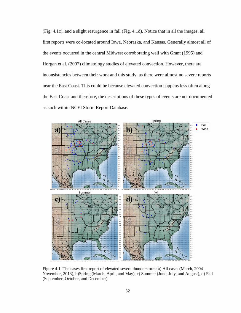
32

(Fig. 4.1c), and a slight resurgence in fall (Fig. 4.1d). Notice that in all the images, all

first reports were co-located around Iowa, Nebraska, and Kansas. Generally almost all of

the events occurred in the central Midwest corroborating well with Grant (1995) and

Horgan et al. (2007) climatology studies of elevated convection. However, there are

inconsistencies between their work and this study, as there were almost no severe reports

near the East Coast. This could be because elevated convection happens less often along

the East Coast and therefore, the descriptions of these types of events are not documented

as such within NCEI Storm Report Database.

Figure 4.1. The cases first report of elevated severe thunderstorm: a) All cases (March, 2004-

November, 2013), b)Spring (March, April, and May), c) Summer (June, July, and August), d) Fall

(September, October, and December)

a) b)

c) d)

33

4.2 Aggregate Results (Statistical Analysis)

As mentioned previously, analysis of all 80 cases of severe elevated

thunderstorms allowed characterization of each event as Marginal or Significant. Cases

were also classified as Hail Dominant, or Wind Dominant. Three cases had an equal

amount of wind and hail reports. In Figure 4.2, a comparison of DCAPE, DCIN,

MUCAPE, and MUCIN are represented in a Box-and-Whisker graphic where only minor

differences between variables in the Significant (N=55) versus Marginal (N=25) case

classes can be seen. Only MUCAPEs seem to be different from one another; even so, the

median values (just under 1000 J kg-1

) are typical of many elevated convection events.

The sameness (both small) of the CINs between case classes suggests an atmosphere very

close to convective overturning. For the downdraft, the DCAPE and DCIN plots for both

case classes look quite similar. It will likely be difficult to show any significant

difference between the samples. Most of the variables studied here (Figure 4.2) do not

have Gaussian distributions. As such, most statistical comparisons between the

Significant and Marginal Case classes was carried out using the non-parametric Mann-

Whitney test.

34

Figure 4.2. Significantly severe (≥5 severe reports) compared to marginally severe (<5 severe

reports) thermodynamic variables of elevated thunderstorms Box-and-Whisker Plot.

Table 4.1. Significant case variables (MUCIN_SIG, MUCAPE_SIG, DCAPE_SIG, and

DCIN_SIG) and marginal case variables (MUCIN_MAR, MUCAPE_ MAR, DCAPE_ MAR,

and DCIN_ MAR) are compared using a Mann-Whitney Test.

MUCIN_SIG to MUCIN_ MAR

MUCAPE_SIG to MUCAPE_

MAR

DCAPE_SIG to

DCAPE_ MAR

DCIN_SIG to DCIN_ MAR

Z-Value -0.954 -0.550 -0.737 -1.677

One-Tail Prob 0.170 0.291 0.231 0.047

After testing, only samples for DCINs from the Significant and Marginal case sets

can be argued to come from different populations (Table 4.1). Indeed, a closer inspection

reveals mean (median) values of DCIN are -53 J kg-1

(-43 J kg-1

) for Marginal cases as

opposed to -50 J kg-1

(-6 J kg-1

) to Significant cases. The skew of the median closer to

zero than the mean is a testament to the more gamma-like distribution of DCIN in both

35

samples. However, the less negative values for the Significant cases are consistent with

the expectation that downdrafts will be able to penetrate to the surface more easily.

Another relationship that is expected is that an increase in MUCAPE will

generally result in a larger DCAPE. This is because the same conditions that lead to

stronger CAPEs for updrafts (warmer temperatures in the lower troposphere and/or

colder temperatures aloft) are also logical ingredients for stronger DCAPE values.

Correlating MUCAPE to DCAPE yields values for the Significant case set of r=0.72

(p<<0.01), and r=0.60 (p<<0.01) for the Marginal case set. The relationship between

these variables in both case sets are shown in Figure 4.3.

Figure 4.3. Scatter plot of Marginal cases (black-dots) and Significant cases (green-squares) are

shown to represent similarities between thunderstorms MUCAPE and DCAPE values measured

in J/kg. Black-dotted line represents a 1:1 ratio of MUCAPE to DCAPE for reference.

36

Now that the statistical analysis of marginally severe and significantly severe

cases have been studied, the cases can now be distinguished by the dominate severe-type

associated with each case. For this dataset, the 3 cases of equal amount of storm type

reports which were eliminated from the analysis. In Figure 4.4, one can see only minor

differences between variables in the Hail (N=61) versus Wind (N=16) case classes.

Mann-Whitney tests were carried out again to determine if there is any significant signal

in the box-and-whisker plots.

Figure 4.4. Box-and-Whisker plots between all hail and wind dominated cases.

With this analysis (Table 4.2), the samples for MUCIN and DCIN from the Hail

Dominant and Wind Dominant case sets can be argued to come from different

populations. Here, the focus is centered on the MUCIN, wherein calculations of mean

37

(median) values of MUCIN are -17 J kg-1

(-1 J kg-1

) for Hail Dominant cases as opposed

to -20 J kg-1

(-6.5 J kg-1

) to Wind Dominant cases. Once again, there is a skewing of the

median MUCIN closer to zero than the mean, indicating more gamma-like distribution of

MUCIN in both samples. The more negative values of MUCIN in the Wind Dominant

case set would suggest a slightly stronger capping inversion, and a stronger updraft

required to break that cap. A stronger downdraft might be expected, although the other

Mann-Whitney results do not support that conclusion for the DCAPE values.

Table 4.2. Hail Dominant case variables (MUCIN-Hail, MUCAPE-Hail, DCAPE-Hail, and

DCIN-Hail) and Wind Dominant case variables (MUCIN-Wind, MUCAPE-Wind, DCAPE-

Wind, and DCIN-Wind) are compared using a Mann-Whitney Test.

MUCIN-Hail to MUCIN-Wind

MUCAPE-Hail to MUCAPE-Wind

DCAPE-Hail to DCAPE-Wind

DCIN-Hail to DCIN-Wind

Z-Value -2.819 -0.226 -0.603 -2.203

One-Tail Prob 0.002 0.411 0.273 0.014

Using Mann-Whitney test again when comparing DCIN/DCAPE ratios of

Significant cases (N=55) versus Marginal cases (N=25) showed a z-value of 1.719 with a

one-tail probability of 0.043. Of the Significant cases (Figure 4.5a), there were 45 hail

cases, 8 wind cases, and 2 cases where there was an equal amount of hail and wind

reports. Of the Marginal cases (Figure 4.5b), there were 16 hail cases, 8 wind cases, and 1

case where there was an equal amount of hail and wind reports. This DCIN/DCAPE ratio

comparison shows that if the ratio is near zero, then it is more likely to be a Significant

case. Furthermore, all Wind Dominant cases were identified as having a DCIN/DCAPE

ratio equal to zero. Shown in Figure 4.5c is the DCIN/DCAPE ratio for the initial report

for Hail Dominant cases, while Figure 4.5d is for Wind Dominant cases. Again, a Mann-

Whitney test was conducted and there was a one-tail probability value of 0.013 of ratios

38

when correlating hail cases to wind. This shows that when DCIN/DCAPE is greater than

zero, then the thunderstorm will be more likely hail dominated.

Figure 4.5. Histograms of DCIN/DCAPE ratio based on initial report of severe weather: a)

Significant cases b) Marginal Cases, c) Hail Dominant cases, d) Wind Dominant cases.

a) b)

c) d)

39

4.3 Case studies

Over the 10-year dataset of elevated convection with characteristics of severe

weather, 80 cases were found. Of the 80 severe cases, 55 cases were significantly (≥ 5

reports) severe and 25 cases were marginally (<5 reports) severe. Figure 4.6 represents

the first severe weather report for each case and the dominating type of severe weather

associated with each case. The study also found 61 of the 80 cases were dominated by

hail while 16 were dominated by wind and 3 had the same number of reports of hail and

wind.

For the case studies, the environments were analyzed to represent 4 different

cases. Each case was chosen based on the number of storm reports. First, there were the

extreme events, in which the Significant case with the most hail (65 reports) and wind (39

reports) were chosen. Secondly, Significant cases with the median number of reports for

wind (8 reports) and hail (10 reports) were selected. Using a forecast funnel method, the

area of interest was analyzed from top to bottom using SPC mesoscale analysis maps and,

finally, the thermodynamics of the environments was evaluated using a skew-T and 2-D

map display.

40

Figure 4.6. First reports location for each case with the dominate type of severe weather

represented by blue-dot (hail) and red-star (wind).

4.3.1 Case 1: Iowa, 29 May 2011

The first case study occurred on 29 May 2011, with the first report of severe

weather at 1121 UTC and is representative of the event with the highest amount of severe

wind reports. As shown in Figure 4.7, the main location of this event was in eastern Iowa.

Overnight, a small elevated MCS developed in western Iowa. As time progressed into the

early morning hours, the MCS traveled from west to east, north of a warm front, and with

an increase in speed. Furthermore, the MCS started producing only hail in eastern

Nebraska/western Iowa. Yet, as it strengthened, the MCS started to produce severe winds

41

in central to eastern Iowa and northern Illinois. A radar image/composite of the elevated

thunderstorm system is shown near its start over central/southern Iowa producing severe

weather (Fig. 4.8).

Figure 4.7. Severe storm reports on 29 May 2011 from 1121 UTC to 1724 UTC. Red circle

represents the first severe report recorded and the location of sounding (Fig. 4.10). Reports were

acquired from the NCEI.

42

Figure 4.8. 2-km resolution base reflectivity radar mosaic on 29 May 2011 at 1200 UTC.

Reproduced from the Storm Prediction Center.

An analysis of the 300-hPa upper level jet revealed the aforementioned area of

concern was within the right entrance region and therefore providing upper-level support

(Figure 4.9a). A strong 500-hPa trough was pushing over the Rocky Mountains putting

Nebraska, Iowa and Illinois in a strong southwest flow (Figure 4.9b). The 850-hPa low-

level jet was oriented south southwesterly and was in excess of 50 knots with the nose of

the low level jet overriding the front into southern Iowa and Nebraska (Figure 4.9c). In

Figure 4.9d a surface analysis is represented. A low pressure system was located in south

west Kansas with a warm front stretching across Kansas, northern Missouri, and central

Illinois. Also, notice the surface observations in central Nebraska and southern Iowa had

easterly winds. Lastly, the 2-km resolution base reflectivity image (Fig. 4.8) shows the

MCS as it propagated to the east while remaining north of the warm front. Using RAOB

software, a skew-T analysis has been created for Madison, Iowa to analyze the wind and

thermodynamic environment (Fig. 4.10). The area with the first report of severe weather

43

was the area of interest for these cases. Notice in the sounding there was strong

directional and speed shear with a veering wind pattern. The winds at the surface were

out of the east. The skew-T also displayed calculated thermodynamic quantities of

downdraft convective available potential energy (DCAPE), downdraft convective

inhibition (DCIN), and most unstable convective available potential energy (MUCAPE).

Figure 4.10 displays the DCAPE values of 538 J/kg, DCIN of 0 J/kg, and MUCAPE of

1,073 J/kg. Figure 4.11 shows a 2-D display of DCAPE and DCIN revealing how the

MCS continues to move east into central Iowa, where the DCAPE increases and DCIN

decreases. This is a more favorable environment for downdraft parcels to push through

the stable layer and reach the surface. The comparison of Figure 4.7 with Figure 4.11

shows a correlation between severe hail reports from eastern Nebraska to central Iowa

turned into mostly severe wind reports from central Iowa into northern Illinois as the

DCIN/DCAPE ratio became progressively closer to zero.

44

Figure 4.9. On 29 May 2011 at 1200 UTC: a) 300-hPa isotachs, streamlines, and divergence,

b)500-hPa observations, heights, and temperatures, c) 850-hPa observations, heights (black-solid

lines), temperatures (red-dotted lines), and moisture (green), d) Surface analysis. Reproduced

from the Storm Prediction Center and Weather Prediction Center.

b)

c) d)

)

SPC

SPC

a)

SPC

WPC

45

Figure 4.10. RAOB sounding analysis for Madison, Iowa on 29 May 2011 at 1100 UTC.

Location represented as red-circle on Figure 4.7

46

Figure 4.11. 29 May 2011 at 1100 UTC 2-D display of DCIN (black-solid lines) and DCAPE

(red-dotted lines) with the addition of DCAPE/DCIN ratio equal to 1 and 2 represented in green

dotted lines. Blue ellipse is representative of where majority of hail reports occurred. Red dashed

ellipse is representative of where majority of wind reports occurred.

4.3.2 Case 2: Kansas/Nebraska/Iowa, 09 April 2013

On the night of 09 April 2013, severe elevated thunderstorms ripped through

Kansas, Iowa, and Nebraska and a combined 63 severe hail reports and 7 severe wind

reports were recorded. In Figure 4.12, all 70 of these reports are represented and were

acquired from the NCEI. This case was the largest hail case that spanned over Kansas,

47

Iowa, and Nebraska. The radar summary at 0310 UTC underscores how wide spread this

event was (Figure 4.13) as the thunderstorms propagated east-northeast

Figure 4.12. Severe storm reports on 09-10 April 2013 from 2300 UTC (04/09/2013) to 0345

UTC (04/10/2013). Red circle represents the first severe report recorded and the location of

sounding (Fig. 4.15). Reports were acquired from the NCEI.

48

Figure 4.13. 2-km resolution base reflectivity radar mosaic on 10 April 2013 at 0310 UTC.


The 0000 UTC upper-air analyses were used in analyzing the upper air

environment and surface analysis for this case. There was a coupling of 300-hPa upper-

level-jets (Kastman et al. 2017) with considerable amounts of divergence recorded over

the area of interest (Figure 4.14a). Additionally in Figure 4.14b, a 500-hPa closed-off low

was centered over Colorado with southwesterly flow. The 850-hPa low-level jet was

active and normal to the associated surface boundary (Figure 4.14c). At the surface, a low

pressure system was located over southeastern Kansas with a stationary front extending

to the northeast along the Missouri/Kansas border to northeastern Missouri (Figure 4.14d)

while a cold front stretched to the south into central Texas. The sounding (Fig. 4.15)

displays a northerly component of wind and a warm air advection signature above 850-

hPa. Additionally, DCAPE was calculated at 519 J/kg, DCIN was 419 J/kg, and

MUCAPE was calculated at 418 J/kg. These storms initiated north of the front within the

49

cold sector and produced severe weather that is concluded by this dataset to be the most

extreme significant hail event. In Figure 4.16, a 2-D display of DCIN and DCAPE shows

considerable amounts of DCIN stretch over most of the area in interest. The

DCAPE/DCIN ratios of ~1 seem to correlate with severe hail reports in Figure 4.12.

However, DCAPE/DCIN values alone should not alone be used in assessing potential

hail case as significant updraft strengths are also essential.

Figure 4.14. On 10 April 2013 at 0000 UTC: a) 300-hPa isotachs, streamlines, and divergence,




a) b)

c) d)

SPC SPC

SPC WPC

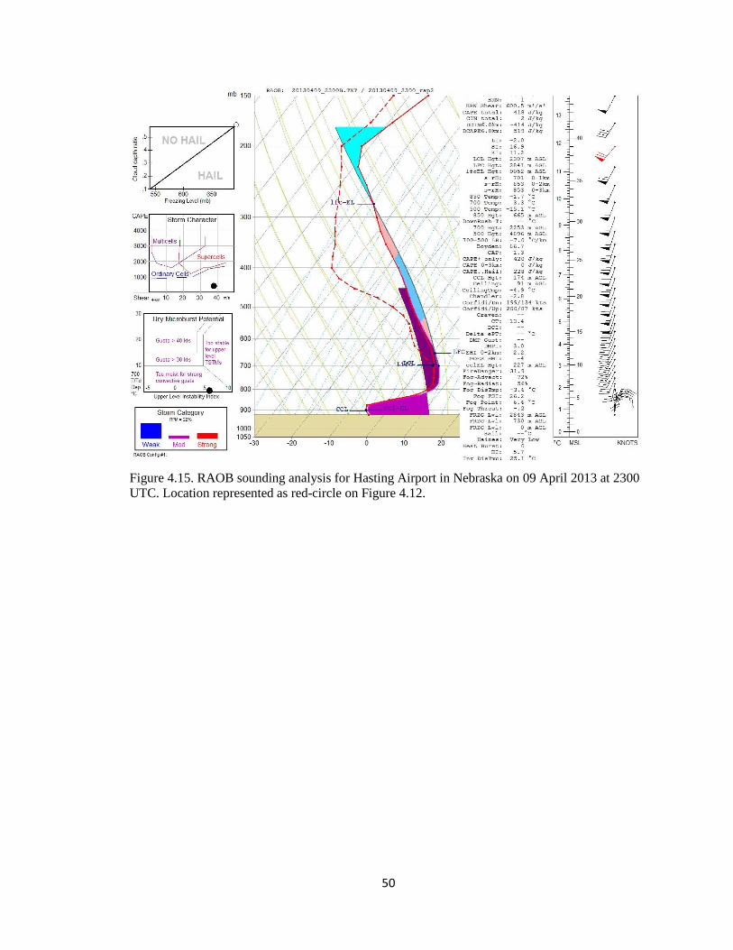
50

Figure 4.15. RAOB sounding analysis for Hasting Airport in Nebraska on 09 April 2013 at 2300

UTC. Location represented as red-circle on Figure 4.12.

51

Figure 4.16. 09 April 2013 at 2300 UTC 2-D display of DCIN (black-solid lines) and DCAPE


dotted lines. Blue ellipse is where majority of hail reports occurred.

52

4.3.3 Case 3: Kansas/Nebraska, 13 July 2009

From 0200 UTC to 0800 UTC on 13 July 2009 elevated convection produced

severe winds and hail. The median of all wind reports from cases of significant-only

severe elevated convective events was calculated. This case was chosen as the median

wind-dominated (more wind reports than hail reports) significant (≥5 total severe reports)

elevated severe thunderstorm. The NCEI storm report database concluded there were 15

total severe weather reports, with 7 severe hail and 8 severe wind reports, shown in

Figure 4.17. Initiation took place in southern/western Kansas, and high reflectivity values

propagated parallel to the boundary (Figure 4.18).

Figure 4.17. Severe storm reports on 13 July 2009 from 0200 UTC to 0800 UTC. Red circle



53

Figure 4.18. 2-km resolution base reflectivity radar mosaic on 13 July 2009 at 0501 UTC.


The environmental make-up of this event was different from the other cases. With

no upper-level support at 300 hPa (Figure 4.19a), the area of interest was centered

downstream from the apex of the ridge at 500 hPa (Figure 4.19b). At 0000 UTC, the 850-

hPa low-level jet was modestly active (Figure 4.19c) and was positioned normal to the

surface boundary, but would strengthen over the next few hours. By 0500 UTC, the radar

summary revealed an elongated MCS moving east-southeast. Just south of the MCS was

a surface low pressure system on the Oklahoma/Kansas border with a warm front

extending to Missouri, where a cold front stretched further east across the Ohio River

Valley (Figure 4.19d). Analysis of the skew-T (Figure 4.20), revealed that this particular

environment had 1,288 J/kg of DCAPE with 0 J/kg of DCIN. Additionally, the updraft

instability had a value of 2,329 J/kg of MUCAPE with a warm air advection signature

and a persistent low-level jet to help initiate thunderstorms. Again, the 2-D map of DCIN

and DCAPE shows very high levels of DCAPE with virtually near-zero values of DCIN

54

(Figure 4.21). It seems to hold true, that large DCAPE values with near zero values seem

to suggest an increase in probability for severe winds.

Figure 4.19. On 13 July 2009 at 0000 UTC: a) 300-hPa isotachs, streamlines, and divergence,




SPC SPC

SPC WPC

a) b)

c) d)

55

Figure 4.20. Skew-T log-P analysis for Winona, Kansas on 13 July 2009 at 0200 UTC. Location

represented as red-circle on Figure 4.17.

56

Figure 4.21. 13 July 2009 at 0200 UTC 2-D display of DCIN (black-solid lines) and DCAPE

(red-dotted lines).

4.3.4 Case 4: Michigan, 10 April 2011

On 10 April 2011 in Michigan at 0945 UTC, the first severe hail report was

recorded. As explained in Section 4.2.3, this case was chosen as the median hail-

dominated significant elevated severe thunderstorm case. There were a total of 11 severe

weather reports with 10 reports being severe hail and 1 report of severe wind shown in

Figure 4.22. The MCS moved from west to east parallel to a surface front and featured

high reflectivity (>50 dBz) values (Figure 4.23). As such the surface boundary remained

south of the reflectivity, keeping the MCS located within the cold sector.

57

Figure 4.22. Severe storm reports 10 April 2011 from 0945 UTC to 1248 UTC. Red circle



Figure 4.23. 2-km resolution base reflectivity radar summary on 10 April 2011 at 1130 UTC.


58

At 300 hPa, the area of interest was within the right entrance region of an

anticyclonically-curved upper level jet, near an area of enhanced divergence (Figure

4.24a). A closed-low at 500 hPa was located in Wyoming, with Michigan near the apex

of a ridge in southwesterly flow (Figure 4.24b). A strong southerly low-level jet was

advecting warm moist air over the boundary into Michigan in Figure 4.24c. In Figure

4.24d, a surface low was located in southern Wisconsin with a warm front extending

southeasterly along the Michigan/Indiana border and through central Ohio. Figure 4.25

displays insufficient amounts of instability with DCAPE= 361 J/kg, DCIN=11 J/kg,

MUCIN= 165 J/kg, and MUCAPE= 110 J/kg. The skew-T also displays a veering wind

pattern with speed shear and strong mid-level winds. With a DCAPE of 361 J/kg and a

DCIN of 11 J/kg, one might expect this case would have been a wind event as the

downdraft (DCIN/DCAPE≈0) would have been able to penetrate below the inversion

layer to produce severe winds at the surface.

However, Figure 4.26 shows how the DCAPE decreased west-to-east across

Michigan, and the DCIN increased. On the western side of Michigan, where the one

severe wind report occurred, higher levels of DCAPE (≈300 J/kg) existed, with near zero

DCIN. The MCS moved into higher values of a DCIN/DCAPE environment toward

central and eastern Michigan where all the reports observed were of severe hail. In other

words, a point-sounding calculation of each respective latitude/longitude reports pre-

convective environment would show a smaller DCIN/DCAPE ratio value over western

Michigan (where the one severe wind was observed) and a progressively increasing

DCIN/DCAPE ratio further east (where the most hail reports were observed). In this case,

59

the 2-D map display of DCIN and DCAPE proved to be a valuable tool in assessing the

downdraft of the environment across an area.

Figure 4.24. On 10 April 2011 at 1200 UTC: a) 300-hPa isotachs, streamlines, and divergence,




a) b)

c) d)

SPC SPC

SPC WPC

60

Figure 4.25. RAOB sounding analysis for Wolf Lake, Michigan on 10 April 2011 at 0900 UTC.

Location represented as red-circle on Figure 4.22.

61

Figure 4.26. 10 April 2011 at 0900 UTC 2-D display of DCIN (black-solid lines) and DCAPE


dotted lines. Blue ellipse is where majority of hail reports occurred.

62

CHAPTER 5. CONCLUSIONS

5.1 Conclusions

Previous studies have shown that elevated severe thunderstorms happen more

often (meeting severe criteria for hail, winds, and tornadoes) than previously thought

(Grant 1995, Horgan et al. 2007). The same studies also show that elevated convection

producing severe weather is mainly associated with hail. Horgan et al. (2007), and the

results of this study, both corroborate that severe hail reports are recorded nearly twice as

frequently as severe winds during elevated convective events. Furthermore, differing

methodologies can also alter conclusions. For example, Colby and Walker (2007)

produced a study on 8 tornadoes that were a result of elevated convection. However, none

of their 8 tornadoes would have met the criteria for this study (they were less than 50

statute miles from the frontal boundary), although, there were a total of 14 tornadoes in

this study that met our criteria and were a result of elevated convection. Still, most of our

elevated severe weather reports largely corroborated location and event-type (hail, wind,

or tornado) climatology studies of elevated convection, where Iowa, Nebraska, and

Kansas were the states with the most severe weather reports; severe hail represented

73.5% of the reports followed by severe winds (25.1%) and then tornadoes (1.5%).

Statistical testing strongly suggests that the DCIN is a smaller value (closer to

zero) in Significant cases as opposed to Marginal cases. Also, similar testing reveals that

the DCIN is again a smaller value (closer to zero) in Wind Dominant as opposed to Hail

Dominant cases. Furthermore, the same Mann Whitney approach showed that as the

63

DCIN/DCAPE ratio approaches zero, then it is more likely to be a Significant case.

Lastly, all Wind Dominant cases were identified as having a DCIN/DCAPE ratio equal to

zero.

The case studies performed in the previous section support the statistical testing,

and highlighted the thermodynamic downdraft environment commonly associated with a

significant elevated convection event with severe winds and severe hail. The 8

Significant severe Wind Dominant events in this study all suggest values of DCAPE to be

much greater than values of DCIN (0 J/kg). However, one can also observe that

DCAPE>>DCIN in a Significant severe Hail Dominant case, as we saw in Case 4.

Indeed, the initial sounding may not indicate the severe mode (hail vs. wind) that may

ultimately dominate an event. This limitation on the single sounding makes the

evaluation of DCIN and DCAPE in 2-D plan view analyses all the more important, as

thunderstorms propagate into other thermodynamic environments with larger/smaller

DCIN and DCAPE values. So, using 2-D plan view DCAPE, DCIN, and DCIN/DCAPE

ratio maps, in conjunction with the skew-T, is the optimum approach for assessing

downdraft environments of severe elevated thunderstorms.

5.2 Future work

These studies could be expanded by using larger time frames, different

observational datasets, and differing methodologies (including, calculating DCAPE in

other ways). Also, one could examine the skew-T analyses of all reports for each case.

This approach would allow more robust analysis of environments of wind reports versus

64

hail reports. Additionally, a comparison of non-severe versus severe elevated convective

environments should be studied. Lastly, highly sampled field studies of severe elevated

convection would prove to be useful to determine the changing thermodynamic profile

and of the weather being observed as it propagates into new locations.

65

APPENDIX A

These are the steps that were taken to calculate DCAPE and DCIN in shell scripting

using GEMPAK.

#!/bin/sh

# Get standard settings

LD_LIBRARY_PATH=/opt/SUNWspro/lib:/usr/X11R6/lib:/usr/lib

export LD_LIBRARY_PATH

rm gemglb.nts

rm last.nts

rm INTRP.log

logfile=INTRP.log

####################################################################

##

# INTRP.csh

#

# Programmers: Patrick Market

# University of Missouri, Atmospheric Science

#

# Written: 10 July 2017

# Edited: 17 July 2017

#

# (c) 2017 FM Software. "Because if it works, it's FM."

#

# Basic interpolation routine from p space to z space.

#

####################################################################

##

#----------------------------------------------------------

# Designate filename,levels,date,and time to be calculated

#----------------------------------------------------------

times="110613_1800_"

#times="061110_1400_ 060307_1700_ 060406_1700_ 060406_1800_

060406_1900_ 061003_1600_ 061003_1700_ 061003_1800_"

#----------------------------------------------------------

# Create grids in ZAGL space from PRES space.

#----------------------------------------------------------

for j in $times

do

time=èxpr $j`

66

dt=èxpr $time : '$......$'`

gdat=èxpr $time : '.......$..$'`

file="20${time}ruc252.gem"

#-----------------------------------------------------------

$GEMEXE/gdvint<<EOF>> $logfile

GDFILE = $file

GDOUTF = $file

GDATTIM = $dt/${gdat}00F000

#GDATTIM = $dt/${gdat}

GVCORD = pres/zagl

GLEVEL = 100-6100-100

MAXGRD =

GAREA = grid

r

EOF

$GEMEXE/gpend

done

67

#!/bin/sh




rm gemglb.nts

rm last.nts

rm DCAPEDCIN1.log

logfile=DCAPEDCIN1.log

####################################################################

##

#

# DCAPEDCIN1.csh

#



#


# Edited:

#

# Phase 1 in the integration of the DCAPE: top and bottom layers

(50 m

# deep for trapezoidal integration); then intermediate layers, from

# 5900 m AGL to 100 m AGL (each 100 m deep) .

#


####################################################################

##

#----------------------------------------------------------


#----------------------------------------------------------

leveltb="6000 0"

levell="5900 5800 5700 5600 5500 5400 5300 5200 5100 5000 4900 4800

4700 4600 4500 4400 4300 4200 4100 4000 3900 3800 3700 3600 3500

3400 3300 3200 3100 3000 2900 2800 2700 2600 2500 2400 2300 2200

2100 2000 1900 1800 1700 1600 1500 1400 1300 1200 1100 1000 900 800

700 600 500 400 300 200 100"

#times="17100518_"

times="110529_1100_"

for j in $times

do

time=èxpr $j`

dt=èxpr $time : '$......$'`

gdat=èxpr $time : '.......$..$'`

68

#file="20${time}rap13km.gem"


#-------------------------------------------------------------------

--

# Create the top and bottom layers for the trapezoidal integration.

# 6000-5900 m AGL and 100-0 m AGL

#-------------------------------------------------------------------

--

for k in $leveltb

do

level=èxpr $k`

$GEMEXE/gddiag<<EOF>> $logfile

GDFILE = $file

GDOUTF = $file


#GDATTIM = $dt/${gdat}00F012

GFUNC = mul(1.0, mul(1.0, mul(gravty, (mul(quo(sub(tvrk,

tmst(thte@6000, pres)), tvrk), 50.0)))

GVCO = zagl

GLEVEL = $level

GRDNAM = dcape1

GPACK = none

r

EOF

$GEMEXE/gpend

done

done

#-------------------------------------------------------------------

--

# Create the intermediate layers, each 100-m deep.

# 5900 m AGL to 200 m AGL

#-------------------------------------------------------------------

--

for j in $times

do

time=èxpr $j`

dt=èxpr $time : '$......$'`

gdat=èxpr $time : '.......$..$'`

#file="20${time}rap13km.gem"


69

for k in $levell

do

level=èxpr $k`


GDFILE = $file

GDOUTF = $file


GFUNC = mul(1.0, mul(1.0, mul(gravty, (mul(quo(sub(tvrk,

tmst(thte@6000, pres)), tvrk), 100.0)))

GVCO = zagl

GLEVEL = $level

GRDNAM = dcape1

GPACK = none

r

EOF

$GEMEXE/gpend

done

done

70

#!/bin/sh




rm gemglb.nts

rm last.nts

rm DCAPE2.log

logfile=DCAPE2.log

####################################################################

##

#

# DCAPE2.csh

#



#


# Edited:

#

# Phase 2 in the integration of the DCAPE: first step to mask out

# negative (DCIN) layers - flag positives with a 1, negatives with

# a zero

#


#

####################################################################

##

#----------------------------------------------------------


#----------------------------------------------------------

levels="6000 5900 5800 5700 5600 5500 5400 5300 5200 5100 5000 4900

4800 4700 4600 4500 4400 4300 4200 4100 4000 3900 3800 3700 3600

3500 3400 3300 3200 3100 3000 2900 2800 2700 2600 2500 2400 2300

2200 2100 2000 1900 1800 1700 1600 1500 1400 1300 1200 1100 1000 900

800 700 600 500 400 300 200 100 0"

times="110410_1000_"

#-------------------------------------------------------------------

-----

# Use the LT function to flag negative (DCIN) values in the column.

#-------------------------------------------------------------------

-----

for j in $times

do

71

time=èxpr $j`

dt=èxpr $time : '$......$'`

gdat=èxpr $time : '.......$..$'`


for k in $levels

do

level=èxpr $k`


GDFILE = $file

GDOUTF = $file


GFUNC = LT(0.00, dcape1)

GVCO = zagl

GLEVEL = $level

GRDNAM = dcape2

GPACK = none

r

EOF

$GEMEXE/gpend

done

done

72

#!/bin/sh




rm gemglb.nts

rm last.nts

rm DCAPE3.log

logfile=DCAPE3.log

####################################################################

##

#

# DCAPE3.csh

#



#


# Edited:

#

# Phase 3 in the integration of the DCAPE: Integration!

#


####################################################################

##

#----------------------------------------------------------


#----------------------------------------------------------

levels="6000 5900 5800 5700 5600 5500 5400 5300 5200 5100 5000 4900

4800 4700 4600 4500 4400 4300 4200 4100 4000 3900 3800 3700 3600

3500 3400 3300 3200 3100 3000 2900 2800 2700 2600 2500 2400 2300

2200 2100 2000 1900 1800 1700 1600 1500 1400 1300 1200 1100 1000 900

800 700 600 500 400 300 200 100 0"

times="110410_1000_"

#-------------------------------------------------------------------

--

# This step masks out any layers of DCIN, where the integral value

of

# DCAPE1 was less than zero. DCIN will be dealt with elsewhere.

#-------------------------------------------------------------------

--

for j in $times

do

time=èxpr $j`

73

dt=èxpr $time : '$......$'`

gdat=èxpr $time : '.......$..$'`


for k in $levels

do

level=èxpr $k`

ltop=èxpr $k + 100`


GDFILE = $file

GDOUTF = $file


GFUNC = mul(dcape1, dcape2)

GVCO = zagl

GLEVEL = $level

GRDNAM = dcape3

GPACK = none

r

EOF

$GEMEXE/gpend

done

done

#-------------------------------------------------------------------

--

# Create a dummy value of zero DCAPE 3 values at 6100 m AGL)

#-------------------------------------------------------------------

--

for j in $times

do

time=èxpr $j`

dt=èxpr $time : '$......$'`

gdat=èxpr $time : '.......$..$'`



GDFILE = $file

GDOUTF = $file


GFUNC = mul(1.0, mul(1.0, mul(dcape1@5900%zagl, 0.0)))

GVCO = zagl

74

GLEVEL = 6100

GRDNAM = dcape

GPACK = none

r

EOF

$GEMEXE/gpend

done

#-------------------------------------------------------------------

--

# Integrate the DCAPE3 values from 6000 m to 0 m AGL from

# the top down to arrive at a DCAPE value at 0 m AGL.

#-------------------------------------------------------------------

--

for j in $times

do

time=èxpr $j`

dt=èxpr $time : '$......$'`

gdat=èxpr $time : '.......$..$'`


for k in $levels

do

level=èxpr $k`



GDFILE = $file

GDOUTF = $file


GFUNC = mul(1.0, mul(1.0, add(dcape@$ltop, dcape3@$level)))

GVCO = zagl

GLEVEL = $level

GRDNAM = dcape

GPACK = none

r

EOF

$GEMEXE/gpend

done

done

75

#!/bin/sh




rm gemglb.nts

rm last.nts

rm DCIN2.log

logfile=DCIN2.log

####################################################################

##

#

# DCIN2.csh

#



#


# Edited:

#

# Phase 2 in the integration of the DCIN: first step to mask out

# negative (DCIN) layers - flag positives with a 0, negatives with

# a 1

#


#

####################################################################

##

#----------------------------------------------------------


#----------------------------------------------------------

levels="6000 5900 5800 5700 5600 5500 5400 5300 5200 5100 5000 4900

4800 4700 4600 4500 4400 4300 4200 4100 4000 3900 3800 3700 3600

3500 3400 3300 3200 3100 3000 2900 2800 2700 2600 2500 2400 2300

2200 2100 2000 1900 1800 1700 1600 1500 1400 1300 1200 1100 1000 900

800 700 600 500 400 300 200 100 0"

times="110410_1000_"

#-------------------------------------------------------------------

-----

# Use the GT function to flag negative (DCIN) values in the column.

#-------------------------------------------------------------------

-----

for j in $times

do

time=èxpr $j`

76

dt=èxpr $time : '$......$'`

gdat=èxpr $time : '.......$..$'`


for k in $levels

do

level=èxpr $k`


GDFILE = $file

GDOUTF = $file


GFUNC = GT(0.00, dcape1)

GVCO = zagl

GLEVEL = $level

GRDNAM = dcin2

GPACK = none

r

EOF

$GEMEXE/gpend

done

done

77

#!/bin/sh




rm gemglb.nts

rm last.nts

rm DCIN3.log

logfile=DCIN3.log

####################################################################

##

#

# DCIN3.csh

#



#


# Edited:

#

# Phase 3 in the integration of the DCIN: Integration!

#


####################################################################

##

#----------------------------------------------------------


#----------------------------------------------------------

levels="6000 5900 5800 5700 5600 5500 5400 5300 5200 5100 5000 4900

4800 4700 4600 4500 4400 4300 4200 4100 4000 3900 3800 3700 3600

3500 3400 3300 3200 3100 3000 2900 2800 2700 2600 2500 2400 2300

2200 2100 2000 1900 1800 1700 1600 1500 1400 1300 1200 1100 1000 900

800 700 600 500 400 300 200 100 0"

#times="120526_0400_ 120526_0800_ 120527_0400_ 120527_0500_

120527_0700_ 120530_2000_ 120619_2100_ 130323_0800_ 130324_0400_

130324_0500_ 130409_2300_ 130410_0100_ 130410_0200_ 130410_0300_

130410_0400_ 130410_0500_ 130410_0600_ 130416_1500_ 130416_1600_

130416_1700_ 130417_0800_ 130418_0100_ 130418_0200_ 130526_1600_

130526_1700_ 131030_1100_"

times="110410_1000_"

#-------------------------------------------------------------------

--

# This step masks out any layers of DCAPE, where the integral value

of

# DCAPE1 was GREATER than zero, and sums the negatives instead

(DCIN).

78

#-------------------------------------------------------------------

--

for j in $times

do

time=èxpr $j`

dt=èxpr $time : '$......$'`

gdat=èxpr $time : '.......$..$'`


for k in $levels

do

level=èxpr $k`



GDFILE = $file

GDOUTF = $file


GFUNC = mul(dcape1, dcin2)

GVCO = zagl

GLEVEL = $level

GRDNAM = dcin3

GPACK = none

r

EOF

$GEMEXE/gpend

done

done

#-------------------------------------------------------------------

--

# Create a dummy value of zero DCAPE 3 values at 6100 m AGL)

#-------------------------------------------------------------------

--

for j in $times

do

time=èxpr $j`

dt=èxpr $time : '$......$'`

gdat=èxpr $time : '.......$..$'`


79


GDFILE = $file

GDOUTF = $file


GFUNC = mul(1.0, mul(1.0, mul(dcape1@5900%zagl, 0.0)))

GVCO = zagl

GLEVEL = 6100

GRDNAM = dcin

GPACK = none

r

EOF

$GEMEXE/gpend

done

#-------------------------------------------------------------------

--

# Integrate the DCAPE3 values from 6000 m to 0 m AGL from

# the top down to arrive at a DCAPE value at 0 m AGL.

#-------------------------------------------------------------------

--

for j in $times

do

time=èxpr $j`

dt=èxpr $time : '$......$'`

gdat=èxpr $time : '.......$..$'`


for k in $levels

do

level=èxpr $k`



GDFILE = $file

GDOUTF = $file


GFUNC = mul(1.0, mul(1.0, add(dcin@$ltop, dcin3@$level)))

GVCO = zagl

GLEVEL = $level

GRDNAM = dcin

GPACK = none

80

r

EOF

$GEMEXE/gpend

done

done

81

#!/bin/sh




#rm gemglb.nts

rm loopyloopratio.nts

rm loopyloopratio.log

logfile=loopyloopratio.log

locs="MI"

times="110410_1000_"

#-------------------------------------------------------------------

--

# This step plots dcin, dcape, and a dcape/dcin ratio on a map

# Red-dotted lines=dcape

# Black-Solid lines=dcin

# Purple-dotted lines=1 and 2 ratio of dcape/dcin

#-------------------------------------------------------------------

--

for j in $times

do

time=èxpr $j`

dt=èxpr $time : '$......$'`

gdat=èxpr $time : '.......$..$'`


#for k in $locs

#do

#loc=èxpr $k`

#level=èxpr $k`

#ltop=èxpr $k + 100`

$GEMEXE/gdcntr<<EOF>> $logfile

GDFILE = $file


GLEVEL = 0

GVCORD = zagl

GFUNC = dcape

GDFILE = 20${time}ruc252.gem

CINT = 100

82

LINE = 2/2/2

MAP = 25

MSCALE = 0

TITLE = 1/-1

DEVICE = psc|20${time}.ps

SATFIL =

RADFIL =

IMCBAR =

PROJ = MER

GAREA = ${locs}

IJSKIP =

CLEAR = YES

PANEL = 0

TEXT = 1

SCALE = 999

LATLON =

HILO =

HLSYM =

CLRBAR =

CONTUR = 0

SKIP = 0

FINT = 0

FLINE = 10-20

CTYPE = C

LUTFIL =

STNPLT =

r

GDFILE = $file


GLEVEL = 0

GVCORD = zagl

GFUNC = dcin


CINT = 50

LINE = 1/1/2

MAP = 1

MSCALE = 0

TITLE = 1/-2


SATFIL =

RADFIL =

IMCBAR =

PROJ = MER

GAREA = ${locs}

IJSKIP =

CLEAR = NO

PANEL = 0

TEXT = 1

SCALE = 999

LATLON =

83

HILO =

HLSYM =

CLRBAR =

CONTUR = 0

SKIP = 0

FINT = 0

FLINE = 10-20

CTYPE = C

LUTFIL =

STNPLT =

r

GDFILE = $file


GLEVEL = 0

GVCORD = zagl

GFUNC = quo(dcape, mul(dcin, -1.0))


CINT = -100000;1;2;;100000

LINE = 7/3/2

MAP = 25

MSCALE = 0

TITLE = 1/-3


SATFIL =

RADFIL =

IMCBAR =

PROJ = MER

GAREA = ${locs}

IJSKIP =

CLEAR = NO

PANEL = 0

TEXT = 1

SCALE = 999

LATLON = 1/10/2/1;1/1;1

HILO =

HLSYM =

CLRBAR =

CONTUR = 0

SKIP = 0

FINT = 0

FLINE = 10-20

CTYPE = C

LUTFIL =

STNPLT =

r

EOF

$GEMEXE/gpend

done

84

REFERENCES

Augustine, J.A., and F. Caracena, 1994: Lower-tropospheric precursors to nocturnal MCS

development over the central United States. Wea. Forecasting,9, 116-135.

Benjamin, S. G., G. A. Grell, J. M. Brown, and T. G. Smirnova, and Coauthors, 2004b:

An hourly assimilation forecast cycle: The RUC. Mon. Wea. Rev., 132, 495–518.

Benjamin, S. G., G. A. Grell, J. M. Brown, and T. G. Smirnova, and Coauthors, 2016: A

North American hourly assimilation and model forecast cycle: The Rapid

Refresh. Mon. Wea. Rev. 144, 1669-1694.

Bosart, L. R., and A. Seimon, 1988: A case study of an unusually intense atmospheric

gravity wave. Mon. Wea. Rev. 116, 1857-1886.

Colby, F. P., Jr., and B. E. Walker, 2007: Tornadoes from elevated convection. Preprints,

22nd Conf. on Weather Analysis and Forecasting and 18th Conference on

Numerical Weather Prediction, Park City, UT, Amer. Meteor. Soc., 7A.8.

Colman, B. R., 1990a: Thunderstorms above frontal surfaces in environments without

positive CAPE: Part I: A climatology. Mon. Wea. Rev., 118, 1103-1121.

Colman, B. R., 1990b: Thunderstorms above frontal surfaces in environments without

positive CAPE. Part II: Organization and instability mechanism. Mon. Wea. Rev.,

118: 1123-1144.

Corfidi, S. F., S. J. Corfidi, and D. M. Schultz, 2008: Elevated convection and

castellanus: Ambiguities, significance, and questions. Wea. Forecasting, 23,

1280-1303.

Djuric, D., 1994: Weather Analysis. Prentice Hall; 304.

Doswell, C. A., and E. N. Rasmussen, 1994: The effect of neglecting the virtual

temperature correction on CAPE calculations. Weather and Forecasting, 9, 625-

629.

Fritsch, J. M., and G. S. Forbes, 2001: Mesoscale convective systems. Severe Convective

Storms, Meteor. Monogr., No. 50, Amer. Meteor. Soc., 323-357.

Gilmore, M. S., and L. J. Wicker, 1998: The influence of midtropospheric dryness on

supercell morphology and evolution. Monthly Weather Review, 126, 943-958.

Glass, F. H., D. L. Ferry, J. T. Moore, and S. M. Nolan, 1995: Characteristics of heavy

convective rainfall events across the mid-Mississippi valley during the warm

85

season: Meteorological conditions and a conceptual model. Preprints, 14th

Conf.

on Weather Forecasting and Analysis, Dallas, TX, Amer. Meteor. Soc., 34-41.

Grant, B. N., 1995: Elevated cold-sector severe thunderstorms: A Preliminary study.

Natl. Wea. Dig., 19(4), 25-31.

Horgan, K. L., D. M. Schultz, J. E. Hales, S. F. Corfidi, and R. H. Johns, 2007: A five-

year climatology of elevated severe convective storms in the United States east of

the Rocky Mountains. Wea. Forecasting, 22, 1031-1044.

Johns, R. H., and C. A. Doswell III, 1992: Severe local storm forecasting. Wea.

Forecasting, 7, 588-612.

Kastman, J. S., L. D. McCoy, P. S. Market, and N. I. Fox, 2017: An example of

synergistic coupling of upper- and lower-level jets associated with flash flooding.

Meteorological Applications, 24, 206-210.

Market, P. S., C. E. Halcomb, and R. L. Ebert, 2002: A climatology of thundersnow

events over the contiguous United States. Wea. Forecasting, 17, 1290-1295.

Market, P. S., S. M. Rochette, J. Shewchuk, R. Difani, J. S. Kastman, C. B. Henson, and

N. I. Fox, 2017: Evaluating elevated convection with the downdraft convection

inhibition. Atmospheric Science Letters, 18, 76-81.

Moore, J. T., and G. E. VanKnowe, 1992: The effect of jet-streak curvature on kinematic

fields. Mon. Wea. Rev., 120, 2429-2441.

Moore, J. T., A. C. Czarnetzki, and P. S. Market, 1998: Heavy precipitation associated

with elevated thunderstorms formed in a convectively unstable layer aloft.

Meteorol. Appl., 5, 373-384.

Moore, J. T., F. H. Glass, C. E. Graves, S. M. Rochette, and M. J. Singer, 2003: The

environment of warm-season elevated thunderstorms associated with heavy

rainfall over the central United States. Wea. Forecasting, 18, 861-878.

Nowotarski, C. J., P. M. Markowski, and Y. P. Richardson, 2011: The characteristics of

numerically simulated supercell storms situated over statistically stable boundary

layers. Mon. Wea. Rev., 139, 3139-3162.

Rochette, S. M., and J. T. Moore, 1996: Initiation of an elevated mesoscale convective

system associated with heavy rainfall. Wea. Forecasting, 11, 443-457.

Rochette, S. M., J. T. Moore, and P. S. Market, 1999: The important of parcel choice in

elevated CAPE computations. Natl. Wea. Dig., 23(4) 20-32.

Schumacher, R. S., 2015: Sensitivity of precipitation accumulation in elevated convective

systems to small changes in low-level moisture. J. Atmos. Sci., 72, 2507-2524.

86

Thompson, R. L., C. M. Mead, and R. Edwards, 2007: Effective storm-relative helicity

and bulk shear in supercell thunderstorm environments. Wea. Forecasting, 22,

102-115.

Wakimoto, R. M., 1982: The life cycle of thunderstorm gust fronts as viewed with

Doppler radar and rawinsonde data. Mon. Wea. Rev., 119, 2511-2513.

Wilson, J. W., and R. D. Roberts, 2006: Summary of convective storm initiation and

evolution during IHOP: Observational and Modeling Perspective. Mon. Wea.

Rev., 134, 23-47.

Documents

ANALYSIS OF SEVERE ELEVATED THUNDERSTORMS USING …weather.missouri.edu/PRECIP/Thesis-Grempler-DCIN.pdfANALYSIS OF SEVERE ELEVATED THUNDERSTORMS USING DCIN AND DCAPE A Thesis Presented