Embed Size (px)
Citation preview
Analysis of quantum error-correcting codes:
symplectic lattice codes and toric codes
Thesis byJames William Harrington
AdvisorJohn Preskill
In Partial Fulfillment of the Requirementsfor the Degree of
Doctor of Philosophy
California Institute of TechnologyPasadena, California
2004
(Defended May 17, 2004)

ii
c© 2004
James William Harrington
All rights Reserved
iii
Acknowledgements
I can do all things through Christ, who strengthens me. Phillipians 4:13 (NKJV)
I wish to acknowledge first of all my parents, brothers, and grandmother for
all of their love, prayers, and support.
Thanks to my advisor, John Preskill, for his generous support of my graduate
studies, for introducing me to the studies of quantum error correction, and for
encouraging me to pursue challenging questions in this fascinating field.
Over the years I have benefited greatly from stimulating discussions on the
subject of quantum information with Anura Abeyesinge, Charlene Ahn, Dave Ba-
con, Dave Beckman, Charlie Bennett, Sergey Bravyi, Carl Caves, Isaac Chenchiah,
Keng-Hwee Chiam, Richard Cleve, John Cortese, Sumit Daftuar, Ivan Deutsch,
Andrew Doherty, Jon Dowling, Bryan Eastin, Steven van Enk, Chris Fuchs, Sho-
hini Ghose, Daniel Gottesman, Ted Harder, Patrick Hayden, Richard Hughes,
Deborah Jackson, Alexei Kitaev, Greg Kuperberg, Andrew Landahl, Chris Lee,
Debbie Leung, Carlos Mochon, Michael Nielsen, Smith Nielsen, Harold Ollivier,
Tobias Osborne, Michael Postol, Philippe Pouliot, Marco Pravia, John Preskill,
Eric Rains, Robert Raussendorf, Joe Renes, Deborah Santamore, Yaoyun Shi, Pe-
ter Shor, Marcus Silva, Graeme Smith, Jennifer Sokol, Federico Spedalieri, Rene
Stock, Francis Su, Jacob Taylor, Ben Toner, Guifre Vidal, and Mas Yamada.
Thanks to Chip Kent for running some of my longer numerical simulations
on a computer system in the High Performance Computing Environments Group
(CCN-8) at Los Alamos National Laboratory. Some simulations were also run on
the Pentium Pro based Beowulf Cluster (naegling) computer system operated by
the Caltech CACR.
I am very grateful for helpful comments from Charlene Ahn, Chris Lee, and
Graeme Smith on draft versions of my thesis chapters.
A special thanks to Francis Su, Winnie Wang, Dawn Yang, and Esther Yong
for working alongside me while I was writing parts of this thesis. Also, thanks to
Robert Dirks for being such a patient and fun bridge partner to play with this

iv
past year, which provided a welcome break from work.
I would like to acknowledge some of the teachers that have encouraged me
and helped lead me to this point: David Crane, Fred DiCesare, Maureen Dinero,
Autumn Finlan, Dan Gauthier, Linda Hagreen, Calvin Howell, David Kraines,
Jane LaVoie, Harold Layton, Claude Meyers, Mary Champagne-Myers, Kate Ross,
Anthony Ruggieri, David Schaeffer, Roxanne Springer, and Stephanos Venakides.
Additionally, I want to acknowledge the sharpening role of the accountabil-
ity partners in my life over the past few years: James Bowen, Isaac Chenchiah,
Brenton Chinn, Gene Chu, Tony Chu, Stephan Ichiriu, Frank Reyes, and Kenji
Shimibukuro. I also appreciate my brothers and sisters in the Sedaqah groups I
have belonged to at Evergreen, as well as my fellow grad students in the Caltech
Christian Fellowship and UCLA Graduate Christian Fellowship.
Soli Deo Gloria.

v
Analysis of quantum error-correcting codes:
symplectic lattice codes and toric codes
by
James William Harrington
In Partial Fulfillment of the
Requirements for the Degree of
Doctor of Philosophy
Abstract
Quantum information theory is concerned with identifying how quantum mechan-
ical resources (such as entangled quantum states) can be utilized for a number
of information processing tasks, including data storage, computation, communi-
cation, and cryptography. Efficient quantum algorithms and protocols have been
developed for performing some tasks (e.g., factoring large numbers, securely com-
municating over a public channel, and simulating quantum mechanical systems)
that appear to be very difficult with just classical resources. In addition to iden-
tifying the separation between classical and quantum computational power, much
of the theoretical focus in this field over the last decade has been concerned with
finding novel ways of encoding quantum information that are robust against er-
rors, which is an important step toward building practical quantum information
processing devices.
In this thesis I present some results on the quantum error-correcting properties
of oscillator codes (also described as symplectic lattice codes) and toric codes.
Any harmonic oscillator system (such as a mode of light) can be encoded with
quantum information via symplectic lattice codes that are robust against shifts in
the system’s continuous quantum variables. I show the existence of lattice codes
whose achievable rates match the one-shot coherent information over the Gaussian
quantum channel. Also, I construct a family of symplectic self-dual lattices and
vi
search for optimal encodings of quantum information distributed between several
oscillators.
Toric codes provide encodings of quantum information into two-dimensional
spin lattices that are robust against local clusters of errors and which require
only local quantum operations for error correction. Numerical simulations of this
system under various error models provide a calculation of the accuracy threshold
for quantum memory using toric codes, which can be related to phase transitions
in certain condensed matter models. I also present a local classical processing
scheme for correcting errors on toric codes, which demonstrates that quantum
information can be maintained in two dimensions by purely local (quantum and
classical) resources.
vii
Contents
1 Introduction 1
1.1 Overview . . . . . . . . . . . . . . . . . . . . . . . . . . . . . . . . 1
1.2 Introduction to quantum error correction . . . . . . . . . . . . . . 2
1.3 Key features of lattices . . . . . . . . . . . . . . . . . . . . . . . . . 6
2 Achievable rates for the Gaussian quantum channel 9
2.1 Abstract . . . . . . . . . . . . . . . . . . . . . . . . . . . . . . . . . 9
2.2 Introduction . . . . . . . . . . . . . . . . . . . . . . . . . . . . . . . 9
2.3 The Gaussian quantum channel . . . . . . . . . . . . . . . . . . . . 11
2.4 Lattice codes for continuous quantum variables . . . . . . . . . . . 16
2.5 Achievable rates from efficient sphere packings . . . . . . . . . . . 20
2.6 Improving the rate . . . . . . . . . . . . . . . . . . . . . . . . . . . 22
2.7 Achievable rates from concatenated codes . . . . . . . . . . . . . . 26
2.8 The Gaussian classical channel . . . . . . . . . . . . . . . . . . . . 33
2.9 Conclusions . . . . . . . . . . . . . . . . . . . . . . . . . . . . . . . 37
3 Family of symplectic self-dual lattice codes 39
3.1 Abstract . . . . . . . . . . . . . . . . . . . . . . . . . . . . . . . . . 39
3.2 Introduction . . . . . . . . . . . . . . . . . . . . . . . . . . . . . . . 39
3.3 Constructing oscillator codes . . . . . . . . . . . . . . . . . . . . . 40
3.4 Program . . . . . . . . . . . . . . . . . . . . . . . . . . . . . . . . . 42
3.4.1 Parameterization . . . . . . . . . . . . . . . . . . . . . . . . 42
3.4.2 Algorithm . . . . . . . . . . . . . . . . . . . . . . . . . . . . 44

viii
3.5 Results . . . . . . . . . . . . . . . . . . . . . . . . . . . . . . . . . . 46
3.6 Error models . . . . . . . . . . . . . . . . . . . . . . . . . . . . . . 50
3.6.1 The square lattice Z2 . . . . . . . . . . . . . . . . . . . . . 50
3.6.2 The hexagonal lattice A2 . . . . . . . . . . . . . . . . . . . 51
3.6.3 The checkerboard lattice D4 . . . . . . . . . . . . . . . . . . 53
3.6.4 Bavard’s symplectic lattice F6 . . . . . . . . . . . . . . . . . 56
3.6.5 The exceptional Lie algebra lattice E8 . . . . . . . . . . . . 56
3.7 Achievable rates . . . . . . . . . . . . . . . . . . . . . . . . . . . . 57
3.8 Conclusion . . . . . . . . . . . . . . . . . . . . . . . . . . . . . . . 60
4 Accuracy threshold for toric codes 61
4.1 Abstract . . . . . . . . . . . . . . . . . . . . . . . . . . . . . . . . . 61
4.2 Introduction . . . . . . . . . . . . . . . . . . . . . . . . . . . . . . . 62
4.3 Models . . . . . . . . . . . . . . . . . . . . . . . . . . . . . . . . . . 65
4.3.1 Random-bond Ising model . . . . . . . . . . . . . . . . . . . 65
4.3.2 Random-plaquette gauge model . . . . . . . . . . . . . . . . 73
4.3.3 Further generalizations . . . . . . . . . . . . . . . . . . . . . 77
4.4 Accuracy threshold for quantum memory . . . . . . . . . . . . . . 78
4.4.1 Toric codes . . . . . . . . . . . . . . . . . . . . . . . . . . . 78
4.4.2 Perfect measurements and the random-bond Ising model . . 84
4.4.3 Faulty measurements and the random-plaquette gauge model 86
4.5 Numerics . . . . . . . . . . . . . . . . . . . . . . . . . . . . . . . . 90
4.5.1 Method . . . . . . . . . . . . . . . . . . . . . . . . . . . . . 90
4.5.2 Random-bond Ising model . . . . . . . . . . . . . . . . . . . 92
4.5.3 Random-plaquette gauge model . . . . . . . . . . . . . . . . 98
4.5.4 Anisotropic random-plaquette gauge model . . . . . . . . . 102
4.5.5 The failure probability at finite temperature . . . . . . . . . 104
4.6 Conclusions . . . . . . . . . . . . . . . . . . . . . . . . . . . . . . . 106
ix
5 Protecting topological quantum information by local rules 109
5.1 Abstract . . . . . . . . . . . . . . . . . . . . . . . . . . . . . . . . . 109
5.2 Introduction . . . . . . . . . . . . . . . . . . . . . . . . . . . . . . . 110
5.3 Robust cellular automata . . . . . . . . . . . . . . . . . . . . . . . 110
5.4 Toric codes and implementation . . . . . . . . . . . . . . . . . . . . 112
5.4.1 Toric code stabilizers . . . . . . . . . . . . . . . . . . . . . . 112
5.4.2 Hardware layout . . . . . . . . . . . . . . . . . . . . . . . . 113
5.4.3 Error model . . . . . . . . . . . . . . . . . . . . . . . . . . . 113
5.5 Processor memory . . . . . . . . . . . . . . . . . . . . . . . . . . . 114
5.5.1 Memory fields . . . . . . . . . . . . . . . . . . . . . . . . . . 114
5.5.2 Memory processing . . . . . . . . . . . . . . . . . . . . . . . 117
5.6 Local rules . . . . . . . . . . . . . . . . . . . . . . . . . . . . . . . 118
5.7 Error decomposition proof . . . . . . . . . . . . . . . . . . . . . . . 124
5.8 Lower bound on accuracy threshold . . . . . . . . . . . . . . . . . . 128
5.8.1 Correction of level-0 errors . . . . . . . . . . . . . . . . . . 128
5.8.2 Correction of higher level errors . . . . . . . . . . . . . . . . 128
5.8.3 Classical errors . . . . . . . . . . . . . . . . . . . . . . . . . 134
5.9 Numerical results . . . . . . . . . . . . . . . . . . . . . . . . . . . . 135
5.10 Conclusion . . . . . . . . . . . . . . . . . . . . . . . . . . . . . . . 137
A Translation of “Hyperbolic families of symplectic lattices” 140
A.1 Introduction . . . . . . . . . . . . . . . . . . . . . . . . . . . . . . . 140
A.2 General study of hyperbolic families . . . . . . . . . . . . . . . . . 143
A.2.1 Symplectic lattices and hyperbolic families . . . . . . . . . 143
A.2.2 Symplectic actions on the families . . . . . . . . . . . . . . 146
A.2.3 Geometric study of lengths . . . . . . . . . . . . . . . . . . 148
A.2.4 Relative eutaxy . . . . . . . . . . . . . . . . . . . . . . . . . 150
A.2.5 Principal length functions. Principal points . . . . . . . . . 153
A.2.6 Dirichlet-Voronoı and Delaunay decompositions (associated
with the principal points) . . . . . . . . . . . . . . . . . . . 156
x
A.2.7 Study in the neighborhood of points. Voronoı’s algorithm
and finitude . . . . . . . . . . . . . . . . . . . . . . . . . . . 161
A.2.8 Morse’s theory . . . . . . . . . . . . . . . . . . . . . . . . . 166
A.3 Examples . . . . . . . . . . . . . . . . . . . . . . . . . . . . . . . . 168
A.3.1 Families An. Forms F2n . . . . . . . . . . . . . . . . . . . . 168
A.3.2 Families An (continued). Forms G2n . . . . . . . . . . . . . 170
A.3.3 Families An (continued). Forms H2n(ϕ) (ϕ ∈ SL2(Z)) . . . 173
A.3.4 Families An (continued). Forms J4m−2 . . . . . . . . . . . . 177
A.3.5 Extremal points of families An for 1 ≤ n ≤ 16 . . . . . . . . 178
A.3.6 An interesting hyperbolic family . . . . . . . . . . . . . . . 183
A.3.7 Other examples . . . . . . . . . . . . . . . . . . . . . . . . . 184

xi
List of Figures
2.1 Two ways to estimate the rate achieved by a lattice code. . . . . . 24
2.2 Rates achieved by concatenated codes, compared to the one-shot
coherent information optimized over Gaussian input states. . . . . 30
2.3 The slowly varying function C2, defined by R = log2(C2/σ2), where
R is the rate achievable with concatenated codes. . . . . . . . . . . 31
2.4 Rates for the Gaussian classical channel achievable with concate-
nated codes, compared to the Shannon capacity. . . . . . . . . . . 36
3.1 The normalizer lattice of the Z2 encoding. . . . . . . . . . . . . . . 52
3.2 The normalizer lattice of the A2 encoding. . . . . . . . . . . . . . . 54
3.3 Failure probability of several lattice codes over the Gaussian channel 57
3.4 Achievable rates of several lattice codes over the Gaussian channel 59
4.1 The chain E of antiferromagnetic bonds (darkly shaded) and the
chain E′ of excited bonds (lightly shaded), in the two-dimensional
random-bond Ising model. . . . . . . . . . . . . . . . . . . . . . . . 68
4.2 The phase diagram of the random-bond Ising model (shown schem-
atically), with the temperature T on the vertical axis and the con-
centration p of antiferromagnetic bonds on the horizontal axis. . . 71
4.3 The check operators of the toric code. . . . . . . . . . . . . . . . . 79
4.4 Site defects and plaquette defects in the toric code. . . . . . . . . . 82
4.5 Basis for the operators that act on the two encoded qubits of the
toric code. . . . . . . . . . . . . . . . . . . . . . . . . . . . . . . . . 83
xii
4.6 An error history shown together with the syndrome history that it
generates, for the toric code. . . . . . . . . . . . . . . . . . . . . . . 87
4.7 The failure probability Pfail as a function of the error probability
p for linear size L = 16, 20, 24, 28, 32, 36, in the two-dimensional
random-bond Ising model. . . . . . . . . . . . . . . . . . . . . . . . 93
4.8 The failure probability Pfail as a function of the error probability
p for linear size L = 15, 19, 23, 27, 31, 35, in the two-dimensional
random-bond Ising model. . . . . . . . . . . . . . . . . . . . . . . . 94
4.9 The failure probability Pfail, with the nonuniversal correction sub-
tracted away, as a function of the scaling variable x = (p−pc0)L1/ν0
for the two-dimensional random-bond Ising model, where pc0 and
ν0 are determined by the best fit to the data. . . . . . . . . . . . . 96
4.10 The failure probability Pfail as a function of the error probabil-
ity p for linear size L = 10, 12, 14, 16, 18, in the three-dimensional
isotropic random-plaquette gauge model. . . . . . . . . . . . . . . . 99
4.11 The failure probability Pfail as a function of the error probabil-
ity p for linear size L = 11, 13, 15, 17, 19, in the three-dimensional
isotropic random-plaquette gauge model. . . . . . . . . . . . . . . . 100
4.12 The failure probability Pfail as a function of the scaling variable
x = (p−pc0)L1/ν0 for the random-plaquette gauge model, where pc0
and ν0 are determined by the best fit to the data. . . . . . . . . . . 101
4.13 A log-log plot of the accuracy threshold curve for varying qubit and
measurement error probabilities p and q. . . . . . . . . . . . . . . . 103
5.1 Examples of level-0 flip errors being corrected. . . . . . . . . . . . 129
5.2 Examples of level-0 measurement errors being corrected. . . . . . . 130
5.3 The mean decay time of quantum memory versus qubit error rate. 136
A.1 All the principal points, ad infinitum, for g = 1, M = ( 1 ). . . . . . 159
A.2 Semi-eutactic points. . . . . . . . . . . . . . . . . . . . . . . . . . . 166
A.3 The families HA3 and HA4. . . . . . . . . . . . . . . . . . . . . . . 182

xiii
List of Tables
3.1 Best-known symplectic self-dual lattices . . . . . . . . . . . . . . . 46
5.1 Processor memory fields for local error correction of toric codes . . 115
A.1 Number of eutactic points in HAn (1 ≤ n ≤ 16). . . . . . . . . . . 179
A.2 Extremal symplectic points in HAn (1 ≤ n ≤ 8) . . . . . . . . . . . 181
A.3 Some examples of perfect symplectic forms . . . . . . . . . . . . . 185
1
Chapter 1
Introduction
1.1 Overview
This thesis analyzes the error-correcting properties of symplectic lattice codes and
toric codes. Section 1.2 provides a brief introduction to quantum error correction
and its terminology. Section 1.3 introduces some key features of lattices.
Chapters 2 and 3 are concerned with oscillator codes (also described as sym-
plectic lattice codes), which encode the states of a finite-dimensional quantum
system into a continuous variable system, such as a mode of light. These codes
are analyzed under a restricted class of the Gaussian quantum channel, where the
continuous variables describing the system of oscillators each receive a random kick
governed by a Gaussian distribution. Chapter 2 calculates achievable rates over
this channel, based on the existence of symplectic lattices with special properties in
a large number of dimensions. Chapter 3 analyzes the error-correcting properties
of specific low-dimensional symplectic lattice codes.
Chapters 4 and 5 are concerned with toric codes, which encode quantum in-
formation in a topological manner on two-dimensional surfaces, so that they are
robust against local clusters of errors. Chapter 4 relates the accuracy thresh-
old of toric codes to the phase transitions of condensed matter systems (namely
the two-dimensional random-bond Ising model and the three-dimensional random-
1.2. Introduction to quantum error correction 2
plaquette gauge model). The threshold for quantum memory is calculated numeri-
cally by running Monte Carlo simulations. Chapter 5 restricts the error processing
to purely local communication and control and demonstrates numerically and an-
alytically that an accuracy threshold still exists for toric codes. Thus, it is possible
to maintain quantum information in a two-dimensional system (such as a lattice
of spins) with only local controls.
Chapters 2 and 4 have previously been published [40, 84]. I have updated the
numerics in Section 4.5 and revised the conclusions in Sections 2.9 and 4.6.
Appendix A contains my rough translation of a paper (written in French) on
symplectic lattices by Christophe Bavard [8]. The mathematical community has
begun researching symplectic lattices over the last decade or so, which interestingly
coincides with the development of quantum error-correcting codes, although these
two forays of study have mostly been unconnected. Bavard is one of the experts
in this field, and it was very helpful to have my numerical search in the space of
symplectic lattices be confirmed by his work.
1.2 Introduction to quantum error correction
Quantum information processing promises the ability to perform certain tasks that
are hard to achieve classically, such as simulating quantum systems [30, 54], factor-
ing large numbers [78], or securely distributing private shared keys for encryption
[10, 79] (without restricting the computational power of an adversary). To carry
out these tasks, we need a quantum system which can be evolved in a controlled
manner while not interacting very much with its environment. Fault-tolerant quan-
tum computation is concerned with designing quantum circuits out of imperfect
components in such a way that when errors inevitably occur, their propagation is
controlled and they are removed in a timely manner, provided that the underlying
errors are restricted to some typical set of errors and that the error rate is below
the accuracy threshold of the system. If the error correction can be done by purely
1.2. Introduction to quantum error correction 3
local controls (in terms of measuring and processing error syndromes), then such
a system should be scalable to handle large tasks.
Quantum bits (called qubits) must be protected against not only bit flips (as in
classical systems) but also phase flips. Qubits can be expressed as a unit vector in
C2, when in a pure state (a state of minimal entropy). A mixed state is expressed
as a 2 × 2 density matrix, which has unit trace and nonnegative eigenvalues. We
can define the states of a qubit in the standard basis |0〉 = ( 10 ) and |1〉 = ( 0
1 ).
The Pauli matrices form a basis of unitary operators acting on a qubit and are
defined in the standard basis by
I =
1 0
0 1
, X =
0 1
1 0
, Y =
0 −i
i 0
, Z =
1 0
0 −1
.
We observe that X|0〉 = |1〉 and X|1〉 = |0〉, so we can interpret X as a bit flip
operator. Also, Z|0〉 = |0〉 and Z|1〉 = −|1〉, so we can interpret Z as a phase flip
operator. Since Y = iXZ, we can interpret Y as both a phase flip and a bit flip.
The Pauli group Pn consists of tensor products of Pauli operators and provides a
basis for unitary operators acting on a system of n qubits:
Pn = 1, i,−1,−i × I,X, Y, Z⊗n
All of these definitions can be generalized to d-dimensional quantum systems,
which we refer to as qudits. Let |0〉, |1〉, . . . , |d− 1〉 be a basis for a qudit system.
Pure states are unit vectors in Cd, and Pauli operators can be expressed in the form
ZaXb for some a, b ∈ Z, where we define X|j〉 = |(j + 1) mod d〉 and Z|j〉 = ωj |j〉
with ω = exp2iπ/d (a dth root of unity). Note that Xd = I = Zd, so there are
d2 distinct Pauli operators of the form ZaXb. The Pauli group is similarly defined
as tensor products of operators of the form ZaXb, along with possible phases. We
can define the weight of a Pauli operator to be the number of qudits on which a
non-identity operation (where a and b are not both zero (mod d)) is being applied.
We can now introduce the stabilizer formalism developed by Gottesman [36].
1.2. Introduction to quantum error correction 4
(All of the quantum error-correcting codes discussed in this thesis fit into the stabi-
lizer description.) We choose an Abelian subgroup of the Pauli group Pn to define
a quantum error-correcting code known as a stabilizer code. Let S1, S2, . . . , Sn−k
be generators of the Abelian subgroup, known as the stabilizer group. Note that
by definition, SaSb = SbSa ∀ a, b. The codespace consists of all n-qudit states |ψ〉
that satisfy Sa|ψ〉 = |ψ〉 ∀ Sa. That is, all of the generators act as the identity
on (and thus stabilize) codewords. The codewords are joint eigenvectors of all of
the stabilizer operators, with eigenvalue 1. It turns out that the dimension of the
codespace is equivalent to that of k encoded qudits. We can repeatedly measure
the Sa operators to verify that the state of the system is within the codespace.
For example, the well-known five-qubit code (which encodes one logical qubit
and protects against arbitrary single qubit errors) has generators
S1 = Z ⊗X ⊗X ⊗ Z ⊗ I
S2 = I ⊗ Z ⊗X ⊗X ⊗ Z
S3 = Z ⊗ I ⊗ Z ⊗X ⊗X
S4 = X ⊗ Z ⊗ I ⊗ Z ⊗X
All sixteen stabilizer operators (including the identity) can be expressed in the
form (S1)c1(S2)c2(S3)c3(S4)c4 for cj ∈ 0, 1. This code has the nice property of
being able to choose generators which are cyclic shifts of one another. In all of the
following, I will drop the explicit tensor products and simply refer to the stabilizer
operators by S1 = ZXXZI, S2 = IZXXZ, and so on.
Consider a Pauli operator Ea that does not commute with at least one stabilizer
element Sb. In particular, suppose that SbEa = ωcEaSb for some integer c (with c
not congruent to 0 (mod d)). We then observe that for any codeword |ψ〉,
Sb (Ea|ψ〉) = (SbEa) |ψ〉 = (ωcEaSb) |ψ〉 = ωcEa (Sb|ψ〉) = ωcEa|ψ〉 .
Therefore, Ea|ψ〉 cannot be in the codespace, since it is an eigenvector of Sb with

1.2. Introduction to quantum error correction 5
eigenvalue ωc, instead of 1. If we initially prepare the system of n qudits into some
superposition of codewords, an application of Ea (which may be an error caused
by the environment or a faulty circuit) moves the system into a state orthogonal
to the codespace, and this action can be detected by measuring Sb. We denote the
outcomes of measuring all of the stabilizer generators as the syndrome of the code.
We can correct a set of errors Ea if they have distinct syndromes.
For example, the five-qubit code has unique nontrivial syndromes for the set
of single-qubit errors XIIII, Y IIII, ZIIII, . . . , IIIIX, IIIIY, IIIIZ. That is,
a different subset of S1, S2, S3, S4 anticommute with each single-qubit error. We
can maintain quantum information in the system as long as no more than one of
the five physical qubits decoheres in between each error correction step.
To analyze the error-correcting properties of a stabilizer code, it is important
to also identify the normalizer group. This is the set of Pauli operators (elements
of Pn) that commute with all of the stabilizer operators. The normalizer group
includes all stabilizer operators, in addition to other Pauli operators. In fact, the
normalizer group has d2k as many elements as the stabilizer group.
There are two main interpretations of the normalizer operators that are not
contained in the stabilizer group. First, any such operator S is a logical operator on
the encoded qudits in the system. We see this by observing that for any codeword
|ψ〉,
Sa
(S|ψ〉
)=(SaS
)|ψ〉 =
(SSa
)|ψ〉 = S (Sa|ψ〉) = S|ψ〉 .
Codewords are mapped to codewords under the action of S. The second inter-
pretation is that of undetectable errors. If the environment were to apply S on
the system, the encoded quantum information could be altered without our even
being able to detect this action.
For example, we can choose generators for the normalizer group of the five-qubit
code to be S1, S2, S3, S4, X, Z, with X = ZZIXI and Z = IXZXI. These last
two are logical operators acting on the encoded qubit. Furthermore, because the
1.3. Key features of lattices 6
minimum weight of a normalizer operator not contained in the stabilizer group is
3 (which we have not proven here), this implies that the distance of the code is 3.
That is, there exist weight-3 errors (such as X and Z) that are undetectable by the
code. Futhermore, some weight-2 errors are indistinguishable (in terms of having
identical syndromes) from weight-1 errors. In general, errors acting on no more
than t qubits can be detected if the stabilizer code has distance at least (t + 1),
and they can be corrected if the distance is at least (2t+ 1).
More in-depth descriptions of quantum error-correcting codes are provided in
[72, 62].
1.3 Key features of lattices
Let us also identify some key features of lattices, which will provide compact
mathematical descriptions of oscillator codes.
Given a set of m basis vectors ~vj ∈ Rn (with m ≤ n), we can define an
m-dimensional lattice as the set of points
L =
m∑
j=1
cj~vj
with cj ∈ Z .
That is, the lattice points are given by every integer combination of basis vectors
(including the origin). We can represent the lattice L by an m× n matrix
M =
←− v1 −→
←− v2 −→...
←− vm −→
whose row vectors provide a basis for the lattice. We can define the determinant
of L to be |detM |.
Sometimes it is helpful to be able to define a lattice within a subspace of a

1.3. Key features of lattices 7
higher-dimensional vector space. However, in all of the examples in Section 3.5,
we will choose m = n.
An important property of a lattice is its minimum distance, which is the small-
est distance between any two lattice points, or equivalently, the norm of the lattice
vector closest to the origin (because the set of lattice points is closed under addition
or subtraction). The minimum distance of L is thus
min~x∈L\~0
√~x · ~x ,
where L \ ~0 denotes the lattice L excluding the origin. In order to properly
compare minimum distances, we restrict ourselves to lattices with determinant
one. Such lattices are sometimes described as self-dual or unimodular.
An active area of mathematical research for over a hundred years has been
to identify which lattices in Rn have the largest minimum distance possible for a
given n. This is closely connected to the problem of finding arrangements of non-
overlapping n-dimensional unit spheres that maximize the enclosed volume of the
spheres (known as the sphere-packing problem), which has broad applications from
fruit packing to data compression to providing better reception for cell phones. If
we scale a lattice (multiply its basis vectors by a common factor) such that the
distance between all lattice points is at least 1, then we can construct such a sphere
packing by placing the centers of n-dimensional unit spheres at all of the lattice
points. The lattice with largest minimum distance will give a sphere packing with
greatest density.
The kissing number problem is also closely related to this area of research. In
this case, we are seeking to maximize the number of n-dimensional unit spheres
that touch (or kiss) a unit sphere centered at the origin, without overlapping. This
is a problem of local geometry, while the sphere-packing problem deals with global
properties of an arrangement. Nevertheless, in some dimensions, both the best
known sphere packing and kissing number arrangements are given by the lattice
with largest minimum distance.

1.3. Key features of lattices 8
Another property of a lattice that will be useful in our work is the Voronoi cell.
This is the region around a lattice point ~x whose interior is closer to ~x than to
any other lattice point. In the square lattice Z2, which consists of the set of points
(a, b) for integers a, b, the Voronoi cell of any lattice point is a square centered at
that point.
In this thesis, we will be interested in symplectic self-dual lattices, whose ba-
sis vectors satisfy an additional constraint, in order to construct quantum error-
correcting codes. Specifically, the symplectic inner product of any pair of lattice
points must be an integer. This will be explained in more detail in the following
chapters. Recent mathematical work [17, 8] has begun to identify how the optimal
minimum distance of symplectic lattices compares with the optimal minimum dis-
tance of all Euclidean lattices. A good overview of symplectic lattices is presented
in [13].

9
Chapter 2
Achievable rates for the Gaussian quantum
channel
2.1 Abstract
We study the properties of quantum stabilizer codes whose finite-dimensional pro-
tected code space is embedded in an infinite-dimensional Hilbert space. The sta-
bilizer group of such a code is associated with a symplectic integral lattice in the
phase space of 2N canonical variables. From the existence of symplectic integral
lattices with suitable properties, we infer a lower bound on the quantum capacity
of the Gaussian quantum channel that matches the one-shot coherent information
optimized over Gaussian input states.
2.2 Introduction
A central problem in quantum information theory is to determine the quantum ca-
pacity of a noisy quantum channel—the maximum rate at which coherent quantum
information can be transmitted through the channel and recovered with arbitrarily
good fidelity [62, 72]. A general solution to the corresponding problem for classical
noisy channels was found by Shannon in the pioneering paper that launched clas-
2.2. Introduction 10
sical information theory [75, 22]. With the development of the theory of quantum
error correction [76, 80], considerable progress has been made toward characteriz-
ing the quantum channel capacity [12], but it remains less well understood than
the classical capacity.
The asymptotic coherent information has been shown to provide an upper
bound on the capacity [74, 7] and a matching lower bound has been conjectured,
but not proven [55]. Unfortunately, the coherent information is not subadditive
[27], so that its asymptotic value is not easily computed. Therefore, it has been
possible to verify the coherent information conjecture in just a few simple cases
[11].
One quantum channel of considerable intrinsic interest is the Gaussian quantum
channel, which might also be simple enough to be analytically tractable, thus
providing a fertile testing ground for the general theory of quantum capacities.
A simple analytic formula for the capacity of the Gaussian classical channel was
found by Shannon [75, 22]. The Gaussian quantum channel was studied by Holevo
and Werner [41], who computed the one-shot coherent information for Gaussian
input states, and derived an upper bound on the quantum capacity.
Lower bounds on the quantum capacity of the Gaussian quantum channel were
established by Gottesman, Kitaev, and Preskill [38]. They developed quantum
error-correcting codes that protect a finite-dimensional subspace of an infinite-
dimensional Hilbert space, and showed that these codes can be used to transmit
high-fidelity quantum information at a nonzero asymptotic rate. In this paper,
we continue the study of the Gaussian quantum channel begun in [38]. Our main
result is that the coherent information computed by Holevo and Werner is in fact
an achievable rate. This result lends nontrivial support to the coherent information
conjecture.
We define the Gaussian quantum channel and review the results of Holevo and
Werner [41] in Section 2.3. In Section 2.4 we describe the stabilizer codes for
continuous quantum variables introduced in [38], which are based on the concept
of a symplectic integral lattice embedded in phase space. In Sections 2.5 and
2.3. The Gaussian quantum channel 11
2.6 we apply these codes to the Gaussian quantum channel, and calculate an
achievable rate arising from lattices that realize efficient packings of spheres in high
dimensions. This achievable rate matches the one-shot coherent information IQ of
the channel in cases where 2IQ is an integer. Rates achieved with concatenated
coding are calculated in Section 2.7; these fall short of the coherent information
but come close. In Section 2.8 we consider the Gaussian classical channel, and
again find that concatenated codes achieve rates close to the capacity. Section 2.9
contains some concluding comments about the quantum capacity of the Gaussian
quantum channel.
2.3 The Gaussian quantum channel
The Gaussian quantum channel is a natural generalization of the Gaussian classical
channel. In the classical case, we consider a channel such that the input x and the
output y are real numbers. The channel applies a displacement to the input by
distance ξ,
y = x+ ξ , (2.1)
where ξ is a Gaussian random variable with mean zero and variance σ2; the prob-
ability distribution governing ξ is
P (ξ) =1√
2πσ2e−ξ2/2σ2
. (2.2)
Similarly, acting on a quantum system described by canonical variables q and
p that satisfy the commutation relation [q, p] = i~, we may consider a quantum
channel that applies a phase-space displacement described by the unitary operator
D(α) = exp(αa† + α∗a
), (2.3)
where α is a complex number, [a, a†] = 1, and q, p can be expressed in terms of a
2.3. The Gaussian quantum channel 12
and a† as
q =
√~2
(a+ a†
), p = −i
√~2
(a− a†
). (2.4)
This quantum channel is Gaussian if α is a complex Gaussian random variable
with mean zero and variance σ2. In that case, the channel is the superoperator
(trace-preserving completely positive map) E that acts on the density operator ρ
according to
ρ→ E(ρ) =1πσ2
∫d2α e−|α|
2/σ2D(α)ρD(α)† . (2.5)
In other words, the position q and momentum p are displaced independently,
q → q + ξq , p→ p+ ξp , (2.6)
where ξq and ξp are real Gaussian random variables with mean zero and variance
σ2 = ~σ2.
To define the capacity, we consider a channel’s nth extension. In the classical
case, a message is transmitted consisting of the n real variables
~x = (x1, x2, . . . , xn) , (2.7)
and the channel applies the displacement
~x→ ~x+ ~ξ , ~ξ = (ξ1, ξ2, . . . , ξn) , (2.8)
where the ξi’s are independent Gaussian random variables, each with mean zero
and variance σ2. A code consists of a finite numberm of n-component input signals
~x(a) , a = 1, 2, . . . ,m (2.9)
and a decoding function that maps output vectors to the index set 1, 2, . . . ,m.
We refer to n as the length of the code.
If the input vectors were unrestricted, then for fixed σ2 we could easily construct
2.3. The Gaussian quantum channel 13
a code with an arbitrarily large number of signals m and a decoding function that
correctly identifies the index (a) of the input with arbitrarily small probability of
error; even for n = 1 we merely choose the distance between signals to be large
compared to σ. To obtain an interesting notion of capacity, we impose a constraint
on the average power of the signal,
1n
∑i
(x
(a)i
)2≤ P , (2.10)
for each a. We say that a rate R (in bits) is achievable with power constraint P
if the there is a sequence of codes satisfying the constraint such that the βth code
in the sequence contains mβ signals with length nβ , where
R = limβ→∞
1nβ
log2mβ , (2.11)
and the probability of a decoding error vanishes in the limit β →∞. The capacity
of the channel with power constraint P is the supremum of all achievable rates.
The need for a constraint on the signal power to define the capacity of the
Gaussian classical channel can be understood on dimensional grounds. The clas-
sical capacity (in bits) is a dimensionless function of the variance σ2, but σ2 has
dimensions. Another quantity with the dimensions of σ2 is needed to construct a
dimensionless variable, and the power P fills this role.
In contrast, no power constraint is needed to define the quantum capacity of the
quantum channel. Rather, Planck’s constant ~ enables us to define a dimensionless
variance σ2 = σ2/~, and the capacity is a function of this quantity. In the quantum
case, a code consists of an encoding superoperator that maps an m-dimensional
Hilbert space Hm into the infinite-dimensional Hilbert space H⊗N of N canonical
quantum systems, and a decoding superoperator that maps H⊗N back to Hm. We
say that the rate R (in qubits) is achievable if there is a sequence of codes such
that
R = limβ→∞
1Nβ
log2mβ , (2.12)
2.3. The Gaussian quantum channel 14
where arbitrary states in Hm can be recovered with a fidelity that approaches 1
as β →∞. The quantum capacity CQ of the channel is defined as the supremum
of all achievable rates.
Holevo and Werner [41] studied a more general Gaussian channel that includes
damping or amplification as well as displacement. However, we will confine our
attention in this paper to channels that apply only displacements. Holevo and
Werner derived a general upper bound on the quantum capacity by exploiting the
properties of the “diamond norm” (norm of complete boundedness) of a superop-
erator. The diamond norm is defined as follows: First we define the trace norm of
an operator X as
‖X‖tr ≡ tr√X†X , (2.13)
which for a self-adjoint operator is just the sum of the absolute values of the
eigenvalues. Then a norm of a superoperator E can be defined as
‖E‖so = supX 6=0
‖E(X)‖tr‖X‖tr
. (2.14)
The superoperator norm is not stable with respect to appending an ancillary sys-
tem on which E acts trivially. Thus we define the diamond norm of E as
‖E‖ = supn‖E ⊗ In‖so , (2.15)
where In denotes the n-dimensional identity operator. (This supremum is always
attained for some n no larger than the dimension of the Hilbert space on which
E acts.) Holevo and Werner showed that the quantum capacity obeys the upper
bound
CQ(E) ≤ log2 ‖E T‖ , (2.16)
where T is the transpose operation defined with respect to some basis. In the case
of the Gaussian quantum channel, they evaluated this expression, obtaining
CQ(σ2) ≤ log2
(~/σ2
)(2.17)
2.3. The Gaussian quantum channel 15
for ~/σ2 > 1, and CQ(σ2) = 0 for ~/σ2 ≤ 1.
Holevo and Werner [41] also computed the coherent information of the Gaussian
quantum channel for a Gaussian input state. To define the coherent information
of the channel E with input density operator ρ, one introduces a reference system
R and a purification of ρ, a pure state |Φ〉 such that
trR (|Φ〉〈Φ|) = ρ . (2.18)
Then the coherent information IQ is
IQ(E , ρ) = S (E(ρ))− S (E ⊗ IR(|Φ〉〈Φ|)) , (2.19)
where S denotes the Von Neumann entropy,
S(ρ) = −tr (ρ log2 ρ) . (2.20)
It is conjectured [55, 74, 7] that the quantum capacity is related to the coherent
information by
CQ(E) = limn→∞
1n· Cn(E) , (2.21)
where
Cn(E) = supρIQ(E⊗n, ρ) . (2.22)
Unlike the mutual information that defines the classical capacity, the coherent
information is not subadditive in general, and therefore the quantum capacity
need not coincide with the “one-shot” capacity C1. Holevo and Werner showed
that for the Gaussian quantum channel, the supremum of IQ over Gaussian input
states is
(IQ)max = log2(~/eσ2) (2.23)
(where e = 2.71828..) for ~/eσ2 > 1, and (IQ)max = 0 for ~/eσ2 ≤ 1. According
to the coherent-information conjecture, eq. (2.23) should be an achievable rate.

2.4. Lattice codes for continuous quantum variables 16
2.4 Lattice codes for continuous quantum variables
The lattice codes developed in [38] are stabilizer codes [35, 18] that embed a finite-
dimensional code space in the infinite-dimensional Hilbert space of N “oscillators,”
a system described by 2N canonical variables q1, q2, . . . qN , p1, p2, . . . , pN . That is,
the code space is the simultaneous eigenstate of 2N commuting unitary operators,
the generators of the code’s stabilizer group. Each stabilizer generator is a Weyl
operator, a displacement in the 2N -dimensional phase space.
Such displacements can be parametrized by 2N real numbers α1, α2, . . . , αN ,
β1, β2, . . . , βN , and expressed as
U(α, β) = exp
[i√
2π
(N∑
i=1
αipi + βiqi
)]. (2.24)
Two such operators obey the commutation relation
U(α, β)U(α′, β′) = e2πiω(αβ,α′β′)U(α′, β′)U(α, β) , (2.25)
where
ω(αβ, α′β′) ≡ α · β′ − α′ · β (2.26)
is the symplectic form (or symplectic inner product). Thus Weyl operators com-
mute if and only if their symplectic form is an integer.
The 2N generators of a stabilizer code are commuting Weyl operators
U(α(a), β(a)
), a = 1, 2, . . . , 2N . (2.27)
Thus the elements of the stabilizer group are in one-to-one correspondence with
the points of a lattice L generated by the 2N vectors v(a) = (α(a), β(a)). These

2.4. Lattice codes for continuous quantum variables 17
vectors can be assembled into the generator matrix M of L given by
M =
v(1)
v(2)
·
·
v(2N)
. (2.28)
Then the requirement that the stabilizer generators commute, through eq. (2.25),
becomes the condition that the antisymmetric matrix
A = MωMT (2.29)
has integral entries, where MT denotes the transpose of M , ω is the 2N × 2N
matrix
ω =
0 IN
−IN 0
(2.30)
and IN is the N × N identity matrix. If the generator matrix M of a lattice L
has the property that A is an integral matrix, then we will say that the lattice L
is symplectic integral.
Encoded operations that preserve the code subspace are associated with the
code’s normalizer group, the group of phase space translations that commute with
the code stabilizer. The generator matrix of the normalizer is a matrix M⊥ that
can be chosen to be
M⊥ = A−1M , (2.31)
so that
M⊥ωMT = I ; (2.32)
and (M⊥
)ω(M⊥
)T=(A−1
)T. (2.33)

2.4. Lattice codes for continuous quantum variables 18
We will refer to the lattice generated by M⊥ as the symplectic dual L⊥ of the
lattice L.
Another matrix that generates the same lattice as M (and therefore defines a
different set of generators for the same stabilizer group) is
M ′ = RM , (2.34)
where R is an integral matrix with detR = ±1. This replacement changes the
matrix A according to
A→ RART . (2.35)
By Gaussian elimination, an R can be constructed such that
A =
0 D
−D 0
, (2.36)
and (A−1
)T =
0 D−1
−D−1 0
, (2.37)
where D is a positive diagonal integral N × N matrix. In the important special
case of a symplectic self-dual lattice, both A and(A−1
)T are integral matrices;
therefore D = D−1 and the standard form of A is
A =
0 IN
−IN 0
= ω . (2.38)
Hence the generator matrix of a symplectic self-dual lattice can be chosen to be a
real symplectic matrix: MωMT = ω.
If the lattice is rotated, then the generator matrix is transformed as
M →MO , (2.39)
where O is an orthogonal matrix. Therefore, it is convenient to characterize a

2.4. Lattice codes for continuous quantum variables 19
lattice with its Gram matrix
G = MMT , (2.40)
which is symmetric, positive, and rotationally invariant. In the case of a symplectic
self-dual lattice, the Gram matrix G can be chosen to be symplectic, and two
symplectic Gram matrices G and G′ describe the same lattice if
G′ = RGRT , (2.41)
where R is symplectic and integral. Therefore, the moduli space of symplectic
self-dual lattices in 2N dimensions can be represented as
AN = H(2N)/Sp(2N,Z) , (2.42)
where H(2N) denotes the space of real symplectic positive 2N × 2N matrices
of determinant 1. The space AN can also be identified as the moduli space of
principally polarized abelian varieties in complex dimension N [17].
The encoded operations that preserve the code space but act trivially within the
code space comprise the quotient group L⊥/L. The order of this group, the ratio
of the volume of the unit cell of L to that of L⊥, is m2, where m is the dimension
of the code space. The volume of the unit cell of L is |detM | = |detA|1/2 and the
volume of the unit cell of L⊥ is |detM⊥| = |detA|−1/2; therefore the dimension
of the code space is
m = |Pf A| = |detM | = detD , (2.43)
where Pf A denotes the Pfaffian of A, the square root of its determinant. Thus,
a symplectic self-dual lattice, for which |detM | = |detM⊥| = 1, corresponds to
a code with a one-dimensional code space. Given a 2N × 2N generator matrix M
of a symplectic self-dual lattice, we can rescale it as
M →√λM , (2.44)

2.5. Achievable rates from efficient sphere packings 20
where λ is an integer, to obtain the generator matrix of a symplectic integral lattice
corresponding to a code of dimension
m = λN . (2.45)
The rate of this code, then, is
R = log2 λ . (2.46)
When an encoded state is subjected to the Gaussian quantum channel, a phase
space displacement
(~q, ~p)→ (~q, ~p) + (~ξq, ~ξp) (2.47)
is applied. To diagnose and correct this error, the eigenvalues of all stabilizer gen-
erators are measured, which determines the value of (~ξq, ~ξp) modulo the normalizer
lattice L⊥. To recover, a displacement of minimal length is applied that returns
the stabilizer eigenvalues to their standard values, and so restores the quantum
state to the code space. We can associate with the origin of the normalizer lat-
tice its Voronoi cell, the set of points in R2N that are closer to the origin than
to any other lattice site. Recovery is successful if the applied displacement lies
in this Voronoi cell. Thus, we can estimate the likelihood of a decoding error by
calculating the probability that the displacement lies outside the Voronoi cell.
2.5 Achievable rates from efficient sphere packings
One way to establish an achievable rate for the Gaussian quantum channel is to
choose a normalizer lattice L⊥ whose shortest nonzero vector is sufficiently large.
In this Section, we calculate an achievable rate by demanding that the Voronoi cell
surrounding the origin contain all typical displacements of the origin in the limit
of large N . In Sec. V, we will use a more clever argument to improve our estimate
of the rate.

2.5. Achievable rates from efficient sphere packings 21
The volume of a sphere with unit radius in n dimensions is
Vn =πn/2
Γ(
n2 + 1
) , (2.48)
and from the Stirling approximation we find that
Vn ≤(
2πen
)n/2
. (2.49)
It was shown by Minkowski [61] that lattice sphere packings exist in n dimensions
that fill a fraction at least 1/2(n−1) of space. Correspondingly, if the lattice is
chosen to be unimodular, so that its unit cell has unit volume, then kissing spheres
centered at the lattice sites can be chosen to have a radius rn such that
Vn (rn)n ≥ 2−(n−1) , (2.50)
or
r2n ≥14(2/Vn)2/n ≥ n
8πe. (2.51)
This lower bound on the efficiency of sphere packings has never been improved in
the nearly 100 years since Minkowski’s result. More recently, Buser and Sarnak
[17] have shown that this same lower bound applies to lattices that are symplectic
self-dual.
Now consider the case of n = 2N -dimensional phase space. For sufficiently
large n, the channel will apply a phase space translation by a distance which with
high probability will be less than√n(σ2 + ε), for any positive ε. Therefore, a code
that can correct a shift this large will correct all likely errors. What rate can such
a code attain? If the code is a lattice stabilizer code, and the dimension of the
code space is m, then the unit cell of the code’s normalizer lattice has volume
∆ =1m· (2π~)N . (2.52)
Nonoverlapping spheres centered at the sites of the normalizer lattice can be chosen
2.6. Improving the rate 22
to have radius r =√n(σ2 + ε), where
(2πen
)n/2 (n(σ2 + ε)
)n/2 ≥ 1m· 2−n · (2π~)n/2 , (2.53)
or
m ≥(
~4e
(σ2 + ε))N
. (2.54)
The error probability becomes arbitrarily small for large N if eq. (2.54) is satisfied,
for any positive ε. We conclude that the rate
R ≡ 1N· log2m = log2
(~
4eσ2
), (2.55)
is achievable, provided ~/4eσ2 ≥ 1. However, as noted in Sec. III, the rates that
can be attained by this construction (rescaling of a symplectic self-dual lattice)
are always of the form log2 λ, where λ is an integer.
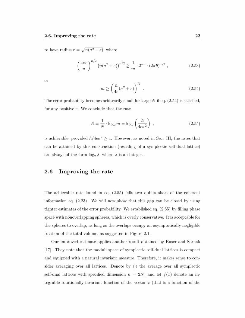
2.6 Improving the rate
The achievable rate found in eq. (2.55) falls two qubits short of the coherent
information eq. (2.23). We will now show that this gap can be closed by using
tighter estimates of the error probability. We established eq. (2.55) by filling phase
space with nonoverlapping spheres, which is overly conservative. It is acceptable for
the spheres to overlap, as long as the overlaps occupy an asymptotically negligible
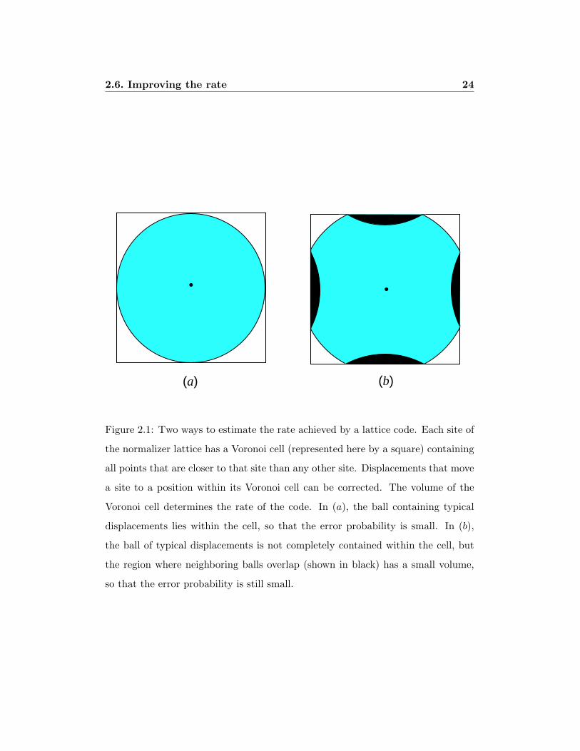
fraction of the total volume, as suggested in Figure 2.1.
Our improved estimate applies another result obtained by Buser and Sarnak
[17]. They note that the moduli space of symplectic self-dual lattices is compact
and equipped with a natural invariant measure. Therefore, it makes sense to con-
sider averaging over all lattices. Denote by 〈·〉 the average over all symplectic
self-dual lattices with specified dimension n = 2N , and let f(x) denote an in-
tegrable rotationally-invariant function of the vector x (that is a function of the
2.6. Improving the rate 23
length |x| of x). Then Buser and Sarnak [17] show that
⟨ ∑x∈L\0
f(x)⟩
=∫f(x) dnx . (2.56)
(Note that the sum is over all nonzero vectors in the lattice L.) It follows that
there must exist a particular symplectic self-dual lattice L such that
∑x∈L\0
f(x) ≤∫f(x) dnx . (2.57)
The statement that a unimodular lattice exists that satisfies eq. (2.57) is the well-
known Minkowski-Hlawka theorem [20]. Buser and Sarnak established the stronger
result that the lattice can be chosen to be symplectic self-dual.
We can use this result to bound the probability of a decoding error, and estab-
lish that a specified rate is achievable. Our argument will closely follow de Buda
[23], who performed a similar analysis of lattice codes for the Gaussian classical
channel. However, the quantum case is considerably easier to analyze, because we
can avoid complications arising from the power constraint [24, 53, 83].
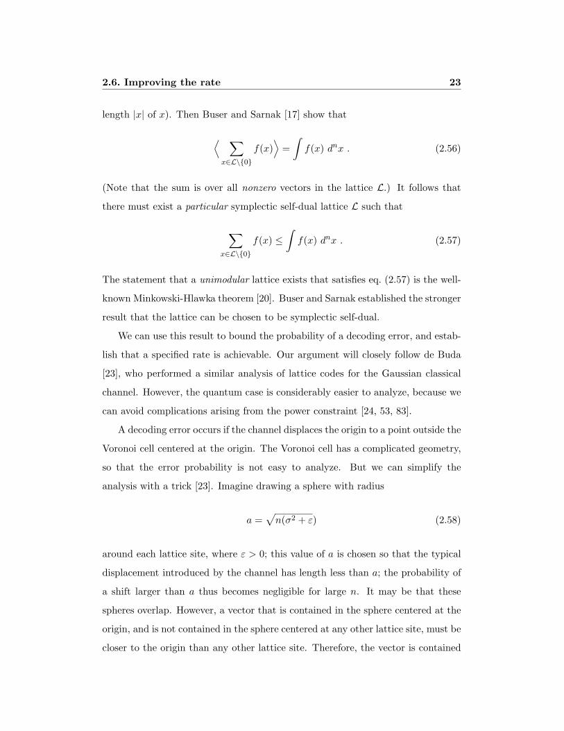
A decoding error occurs if the channel displaces the origin to a point outside the
Voronoi cell centered at the origin. The Voronoi cell has a complicated geometry,
so that the error probability is not easy to analyze. But we can simplify the
analysis with a trick [23]. Imagine drawing a sphere with radius
a =√n(σ2 + ε) (2.58)
around each lattice site, where ε > 0; this value of a is chosen so that the typical
displacement introduced by the channel has length less than a; the probability of
a shift larger than a thus becomes negligible for large n. It may be that these
spheres overlap. However, a vector that is contained in the sphere centered at the
origin, and is not contained in the sphere centered at any other lattice site, must be
closer to the origin than any other lattice site. Therefore, the vector is contained
2.6. Improving the rate 24
(a) (b)
Figure 2.1: Two ways to estimate the rate achieved by a lattice code. Each site of
the normalizer lattice has a Voronoi cell (represented here by a square) containing
all points that are closer to that site than any other site. Displacements that move
a site to a position within its Voronoi cell can be corrected. The volume of the
Voronoi cell determines the rate of the code. In (a), the ball containing typical
displacements lies within the cell, so that the error probability is small. In (b),
the ball of typical displacements is not completely contained within the cell, but
the region where neighboring balls overlap (shown in black) has a small volume,
so that the error probability is still small.

2.6. Improving the rate 25
in the origin’s Voronoi cell, and is a shift that can be corrected successfully. (See
Figure 2.1.)
Hence (ignoring the possibility of an atypical shift by ξ > a) we can upper
bound the probability of error by estimating the probability that the shift moves
any other lattice site into the sphere of radius a around the origin. We then find
Perror ≤∑
x∈L⊥\0
∫|r|≤a
P (x− r)dnr , (2.59)
where P (ξ) denotes the probability of a displacement by ξ.
The Buser-Sarnak theorem [17] tells us that there exists a lattice whose unit cell
has volume ∆, and which is related by rescaling to a symplectic self-dual lattice,
such that
Perror ≤1∆
∫dnx
∫|r|≤a
P (x− r)dnr ; (2.60)
by interchanging the order of integration, we find that
Perror ≤1∆· Vn · an , (2.61)
the ratio of the volume of the n-dimensional sphere of radius a to the volume of
the unit cell.
Now the volume ∆ of the unit cell of the normalizer lattice L⊥, and the di-
mension m of the code space, are related by
∆ = (2π~)Nm−1 =(2π~ · 2−R
)N, (2.62)
where R is the rate, and we may estimate the volume of the sphere as
Vn · an ≤(
2πen
)n/2 (n(σ2 + ε)
)n/2, (2.63)

2.7. Achievable rates from concatenated codes 26
where n = 2N . Thus we conclude that
Perror ≤( e
~(σ2 + ε) · 2R
)N. (2.64)
Therefore, the error probability becomes small for large N for any rate R such
that
R < log2
(~e(σ2 + ε)
), (2.65)
where ε may be arbitrarily small. We conclude that the rate
R = log2
(~eσ2
)(2.66)
is achievable in the limit N →∞, provided that ~/eσ2 > 1. This rate matches the
optimal value eq. (2.23) of the one-shot coherent information for Gaussian inputs.
We note, again, that the rates that we can obtain from rescaling a symplectic self-
dual lattice are restricted to R = log2 λ, where λ is an integer. Thus for specified
σ2, the achievable rate that we have established is really the maximal value of
R = log2 λ , λ ∈ Z , (2.67)
such that the positive integer λ satisfies
λ <~eσ2
. (2.68)
2.7 Achievable rates from concatenated codes
Another method for establishing achievable rates over the Gaussian quantum chan-
nel was described in [38], based on concatenated coding. In each of N “oscillators”
described by canonical variables pi and qi, a d-dimensional system (“qudit”) is en-
coded that is protected against sufficiently small shifts in pi and qi. The encoded
qudit is associated with a square lattice in two-dimensional phase space. Then a

2.7. Achievable rates from concatenated codes 27
stabilizer code is constructed that embeds a k-qudit code space in the Hilbert space
of N qudits; these k encoded qudits are protected if a sufficiently small fraction
of the N qudits are damaged. Let us compare the rates achieved by concatenated
codes to the rates achieved with codes derived from efficient sphere packings.
We analyze the effectiveness of concatenated codes in two stages. First we
consider how likely each of the N qudits is to sustain damage if the underlying
oscillator is subjected to the Gaussian quantum channel. The area of the unit
cell of the two-dimensional square normalizer lattice that represents the encoded
operations acting on the qudit is 2π~/d, and the minimum distance between lattice
sites is δ =√
2π~/d. A displacement of q by a · δ, where a is an integer, is the
operation Xa acting on the code space, and a displacement of p by b · δ is the
operation Zb, where X and Z are the Pauli operators acting on the qudit; these
act on a basis |j〉, j = 0, 1, 2, . . . , d− 1 for the qudit according to
X : |j〉 → |j + 1 (mod d)〉 ,
Z : |j〉 → wj |j〉 , (2.69)
where ω = exp(2πi/d).
Shifts in p or q can be corrected successfully provided that they satisfy
|∆q| < δ/2 =
√π~2d
, |∆p| < δ/2 =
√π~2d
. (2.70)
If the shifts in q and p are Gaussian random variables with variance σ2, then
the probability that a shift causes an uncorrectable error is no larger than the
probability that the shift exceeds√π~/2d, or
pX , pZ ≤ 2 · 1√2πσ2
∫ ∞
√π~/2d
dxe−x2/2σ2
= erfc(√π~/4dσ2) , (2.71)
where erfc denotes the complementary error function. Here pX is the probability

2.7. Achievable rates from concatenated codes 28
of an “X error” acting on the qudit, of the form Xa for a 6≡ 0 (mod d), and pZ
denotes the probability of a “Z error” of the form Zb for b 6≡ 0 (mod d). The
X and Z errors are uncorrelated, and errors with a, b = ±1 are much more likely
than errors with |a|, |b| > 1. By choosing d ∼ ~/σ2, we can achieve a small error
probability for each oscillator.
The second stage of the argument is to determine the rate that can be achieved
by a qudit code if pX and pZ satisfy eq. (2.71). We will consider codes of the
Calderbank-Shor-Steane (CSS) type, for which the correction of X errors and Z
errors can be considered separately [19, 81]. A CSS code is a stabilizer code, in
which each stabilizer generator is either a tensor product of I’s and powers of Z
(measuring these generators diagnoses the X errors) or a tensor product of I’s and
powers of X (for diagnosing the Z errors).
We can establish an achievable rate by averaging the error probability over
CSS codes; we give only an informal sketch of the argument. Suppose that we fix
the block size N and the number of encoded qudits k. Now select the generators
of the code’s stabilizer group at random. About half of the N−k generators are of
the Z type and about half are of the X type. Thus the number of possible values
for the eigenvalues of the generators of each type is about
d12(N−k) . (2.72)
Now we can analyze the probability that an uncorrectable X error afflicts the
encoded quantum state (the probability of an uncorrectable Z error is analyzed in
exactly the same way). Suppose that X errors act independently on the N qudits
in the block, with a probability of error per qudit of pX . Thus for large N , the
typical number of damaged qudits is close to pX · N . A damaged qudit can be
damaged in any of d− 1 different ways (Xa, where a = 1, 2, . . . , (d− 1)). We will
suppose, pessimistically, that all d − 1 shifts of the qudit are equally likely. The
actual situation that arises in our concatenated coding scheme is more favorable—
small values of |a| are more likely—but our argument will not exploit this feature.

2.7. Achievable rates from concatenated codes 29
Thus, with high probability, the error that afflicts the block will belong to a
typical set of errors that contains a number of elements close to
Ntyp ∼
N
NpX
(d− 1)NpX ∼ dN(Hd(pX)+pX logd(d−1)) , (2.73)
where
Hd(p) = −p logd p− (1− p) logd(1− p) . (2.74)
If a particular typical error occurs, then recovery will succeed as long as there is
no other typical error that generates the same error syndrome. It will be highly
unlikely that another typical error has the same syndrome as the actual error,
provided that the number of possible error syndromes d12(N−k) is large compared
to the number of typical errors. Therefore, the X errors can be corrected with
high probability for
12
(1− k
N
)>
1N· logdNtyp ∼ Hd(pX) + pX logd(d− 1) , (2.75)
or for a rate Rd in qudits satisfying
Rd ≡k
N< 1− 2Hd(pX)− 2pX logd(d− 1) (2.76)
Similarly, the Z errors can be corrected with high probability by a random CSS
code if the rate satisfies
Rd < 1− 2Hd(pZ)− 2pZ logd(d− 1) . (2.77)
Converted to qubits, the rate becomes
R = log2 d ·Rd (2.78)
2.7. Achievable rates from concatenated codes 30
0
1
2
3
4
5
6
7
Rate
0 0.1 0.2 0.3 0.4 0.5 0.6σ
CoherentInformation
ConcatenatedCodes
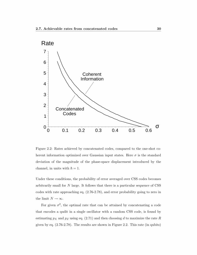
Figure 2.2: Rates achieved by concatenated codes, compared to the one-shot co-
herent information optimized over Gaussian input states. Here σ is the standard
deviation of the magnitude of the phase-space displacement introduced by the
channel, in units with ~ = 1.
Under these conditions, the probability of error averaged over CSS codes becomes
arbitrarily small for N large. It follows that there is a particular sequence of CSS
codes with rate approaching eq. (2.76-2.78), and error probability going to zero in
the limit N →∞.
For given σ2, the optimal rate that can be attained by concatenating a code
that encodes a qudit in a single oscillator with a random CSS code, is found by
estimating pX and pZ using eq. (2.71) and then choosing d to maximize the rate R
given by eq. (2.76-2.78). The results are shown in Figure 2.2. This rate (in qubits)

2.7. Achievable rates from concatenated codes 31
0
0.1
0.2
0.3
0.4
C2
.001 .01 .1σ
Figure 2.3: The slowly varying function C2, defined by R = log2(C2/σ2), where
R is the rate achievable with concatenated codes. Units have been chosen such
that ~ = 1. The horizontal lines are at C2 = 1/e, corresponding to a rate equal
to the coherent information, and at C2 = 1/2e, corresponding to one qubit below
the coherent information.
2.7. Achievable rates from concatenated codes 32
can be expressed as
R = log2
(C2~/σ2
), (2.79)
where C2 is a slowly varying function of σ2/~ plotted in Figure 2.3. It turns out
that this rate is actually fairly close to log2 d; that is, the optimal dimension d of
the qudit encoded in each oscillator is approximately C2~/σ2. With this choice
for d, the error rate for each oscillator is reasonably small, and the random CSS
code reduces the error probability for the encoded state to a value exponentially
small in N at a modest cost in rate. The rate achieved by concatenating coding
lies strictly below the coherent information IQ, but comes within one qubit of IQ
for σ2 > 1.88× 10⁻⁴.
Both the concatenated codes and the codes derived from efficient sphere pack-
ings are stabilizer codes, and therefore both are associated with lattices in 2N -
dimensional phase space. But while the sphere-packing codes have been chosen so
that the shortest nonzero vector on the lattice is large relative to the size of the
unit cell, the concatenated codes correspond to sphere packings of poor quality.
For the concatenated codes, the shortest vector of the normalizer lattice has length
`, where
`2 = 2π~/d (2.80)
and the rate R is close to log2 d. The efficient sphere packings have radius r = `/2
close to√nσ2, or
`2 =8N~e· 2−R . (2.81)
Hence, if we compare sphere-packing codes and concatenated codes with compa-
rable rates, the sphere-packing codes have minimum distance that is larger by a
factor of about√
4N/πe. The concatenated codes achieve a high rate not because
the minimum distance of the lattice is large, but rather because the decoding
procedure exploits the hierarchical structure of the code.

2.8. The Gaussian classical channel 33
2.8 The Gaussian classical channel
We have found that quantum stabilizer codes based on efficient sphere packings can
achieve rates for the Gaussian quantum channel that match the one-shot coherent
information, and that concatenated codes achieve rates that are below, but close
to, the coherent information. Now, as an aside, we will discuss the corresponding
statements for the Gaussian classical channel. We will see, in particular, that
concatenated codes achieve rates that are close to the classical channel capacity.
Shannon’s expression for the capacity of the Gaussian classical channel can
be understood heuristically as follows [75, 22]. If the input signals have average
power P , which is inflated by the Gaussian noise to P +σ2, then if n real variables
are transmitted, the total volume occupied by the space of output signals is the
volume of a sphere of radius√n(P + σ2), or
total volume = Vn ·(n(P + σ2)
)n/2. (2.82)
We will decode a received message as the signal state that is the minimal distance
away. Consider averaging over all codes that satisfy the power constraint and have
m signals. When a message is received, the signal that was sent will typically
occupy a decoding sphere of radius√
(n(σ2 + ε) centered at the received message,
which has volume
decoding sphere volume = Vn ·(n(σ2 + ε)
)n/2. (2.83)
A decoding error can arise if another one of the m signals, aside from the one
that was sent, is also contained in the decoding sphere. The probability that a
randomly selected signal inside the sphere of radius√n(P + σ2) is contained in a
particular decoding sphere of radius√n(σ2 + ε) is the ratio of the volume of the
spheres, so the probability of a decoding error can be upper bounded by m times

2.8. The Gaussian classical channel 34
that ratio, or
Perror < m ·(σ2 + ε
σ2 + P
)n/2
=(
22R · σ2 + ε
σ2 + P
)n/2
, (2.84)
where R is the rate of the code. If the probability of error averaged over codes
and signals satisfies this bound, there is a particular code that satisfies the bound
when we average only over signals. If Perror < δ when we average over signals, then
we can discard at most half of all the signals (reducing the rate by at most 1/n
bits) to obtain a new code with Perror < 2δ for all signals. Since ε can be chosen
arbitrarily small for sufficiently large n, we conclude that there exist codes with
arbitrarily small probability of error and rate R arbitrarily close to
C =12
log2
(1 +
P
σ2
), (2.85)
which is the Shannon capacity. Conversely, for any rate exceeding C, the decod-
ing spheres inevitably have nonnegligible overlaps, and the error rate cannot be
arbitrarily small.
Suppose that, instead of Shannon’s random coding, we use a lattice code based
on an efficient packing of spheres. In this case, the power constraint can be imposed
by including as signals all lattice sites that are contained in an n-dimensional ball
of radius√nP , and the typical shifts by distance
√nσ2 must be correctable. Thus
decoding spheres of radius√nσ2 are to be packed into a sphere of total radius√
n(P + σ2). Suppose that the lattice is chosen so that nonoverlapping spheres
centered at the lattice sites fill a fraction at least 2−(n−1) of the total volume; the
existence of such a lattice is established by Minkowski’s estimate [61]. Then the
number m of signals satisfies
m · Vn · (nσ2)n/2 ≥ 2−(n−1) · Vn ·(n(P + σ2)
)n/2, (2.86)

2.8. The Gaussian classical channel 35
or
m ≥ 2−n
(1 +
P
σ2
)n/2
, (2.87)
corresponding to the rate
R ≡ 1n· log2m =
12
log2
(1 +
P
σ2
)− 1 , (2.88)
which is one bit less than the Shannon capacity.
Much as in the discussion of quantum lattice codes in Sec. 2.6, an improved
estimate of the achievable rate is obtained if we allow the decoding spheres to
overlap [23, 24, 53, 83]. In fact, there are classical lattice codes with rate arbitrarily
close to the capacity, such that the probability of error, averaged over signals, is
arbitrarily small [83]. Unfortunately, though, because of the power constraint, the
error probability depends on which signal is sent, and the trick of deleting the
worst half of the signals would destroy the structure of the lattice. Alternatively,
it can be shown that for any rate
R <12
log2(P/σ2) , (2.89)
there are lattice codes with maximal probability of error that is arbitrarily small
[23]. This achievable rate approaches the capacity for large P/σ2.
Now consider the rates that can be achieved for the Gaussian classical channel
with concatenated coding. A d-state system (dit) is encoded in each of n real
variables. If each real variable takes one of d possible values, with spacing 2∆x
between the signals, then a shift by ∆x can be corrected. By replacing the sum
over d values by an integral, which can be justified for large d, we find an average
power per signal
P ∼ 12d∆x
∫ d∆x
−d∆xx2dx =
13(d∆x)2 ; (2.90)
thus the largest correctable shift can be expressed in terms of the average power
2.8. The Gaussian classical channel 36
0
1
2
3
4
5
6
7
Rate
0 0.1 0.2 0.3 0.4 0.5 0.6σ
ShannonCapacity
ConcatenatedCodes
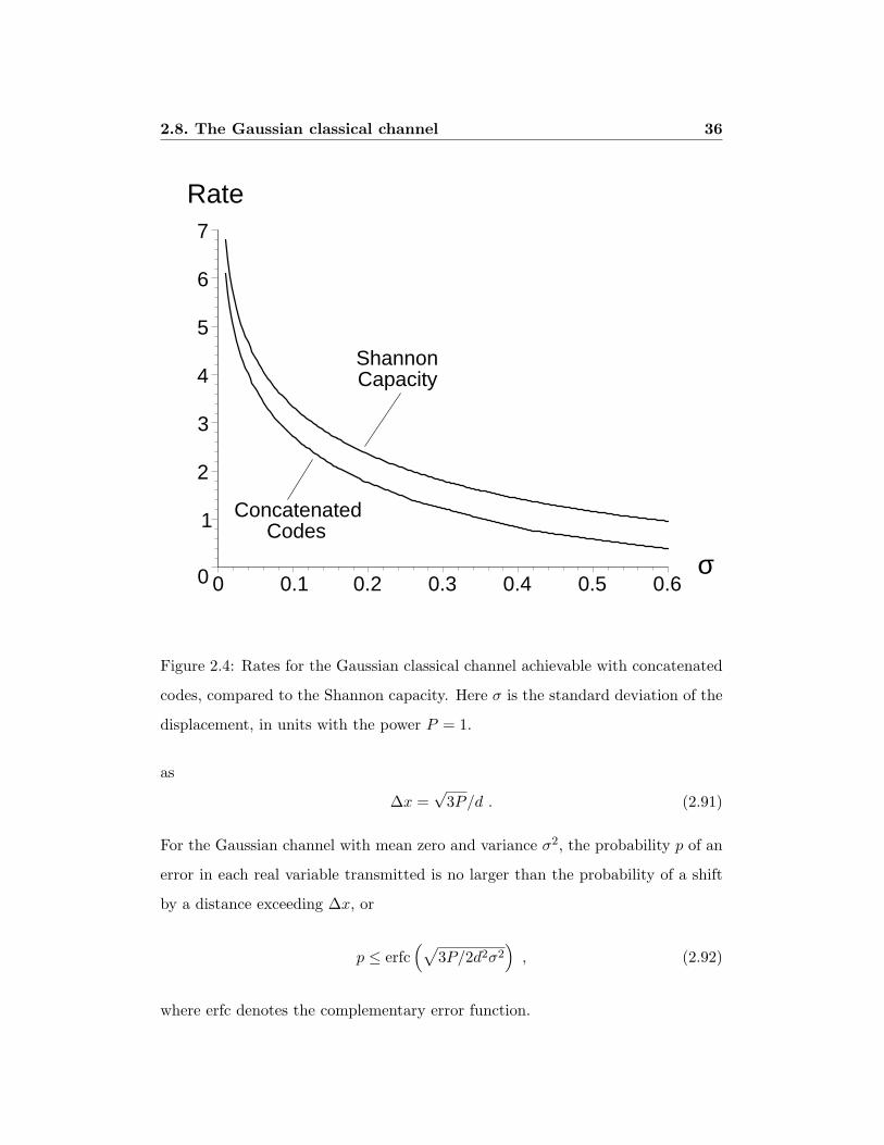
Figure 2.4: Rates for the Gaussian classical channel achievable with concatenated
codes, compared to the Shannon capacity. Here σ is the standard deviation of the
displacement, in units with the power P = 1.
as
∆x =√
3P/d . (2.91)
For the Gaussian channel with mean zero and variance σ2, the probability p of an
error in each real variable transmitted is no larger than the probability of a shift
by a distance exceeding ∆x, or
p ≤ erfc(√
3P/2d2σ2), (2.92)
where erfc denotes the complementary error function.

2.9. Conclusions 37
We reduce the error probability further by encoding k < n dits in the block
of n dits. Arguing as in Sec. 2.7, we see that a random code for dits achieves an
asymptotic rate in bits given by
R = log2 d · (1−Hd(p)− p logd(d− 1)) . (2.93)
Given σ2, using the expression eq. (2.92) for p, and choosing d to optimize the rate
in eq. (2.93), we obtain a rate close to the Shannon capacity, as shown in Figure
2.4. As for the concatenated quantum code, the rate of the concatenated classical
code is close to log2 d, where d ∼ C(σ2) ·√P/σ2, and C(σ2) is a slowly varying
function.
2.9 Conclusions
We have described quantum stabilizer codes, based on symplectic integral lattices
in phase space, that protect quantum information carried by systems described by
continuous quantum variables. With these codes, we can establish lower bounds
on the capacities of continuous-variable quantum channels.
For the Gaussian quantum channel, the best rate we know how to achieve
with stabilizer coding matches the one-shot coherent information optimized over
Gaussian inputs, at least when the value of the coherent information is log2 of
an integer. That our achievable rate matches the coherent information only for
isolated values of the noise variance σ2 seems to be an artifact of our method of
analysis, rather than indicative of any intrinsic property of the channel. Hence it is
tempting to speculate that this optimal one-shot coherent information actually is
the quantum capacity of the channel. Sam Thomsen continued this line of work as
a SURF project during the summer of 2002. He found a way to modify the Buser-
Sarnak theorem [17] that seems to show the existence of symplectic lattices whose
achievable rates would match the coherent information everywhere our proof is

2.9. Conclusions 38
valid (specifically, for small σ).
Conceivably, better rates can be achieved with nonadditive quantum codes that
cannot be described in terms of symplectic integral lattices. We don’t know much
about how to construct these codes, or about their properties.
In the case of the depolarizing channel acting on qubits, Shor and Smolin dis-
covered that rates exceeding the one-shot coherent information could be achieved.
Their construction used concatenated codes, where the “outer code” is a random
stabilizer code, and the “inner code” is a degenerate code with a small block size
[27]. The analogous procedure for the Gaussian channel would be to concatenate
an outer code based on a symplectic integral lattice with an inner code that en-
codes one logical oscillator in a block of several oscillators. This inner code, then,
embeds an infinite-dimensional code space in a larger infinite-dimensional space,
as do codes constructed by Braunstein [16] and Lloyd and Slotine [56]. However,
we have not been able to find concatenated codes of this type that achieve rates
exceeding the one-shot coherent information of the Gaussian channel.

39
Chapter 3
Family of symplectic self-dual lattice codes
3.1 Abstract
The continuous variable quantum error-correcting codes introduced in [38] pro-
vide a means for robustly storing and processing quantum information in systems
described by harmonic oscillators, such as a mode of light. These codes protect
the encoded information from random kicks to the oscillator variables, provided
that the magnitude of the kicks is not too strong. In this work, we present several
explicit encodings and calculate their achievable rates over the Gaussian quantum
channel. These encodings were found by searching for symplectic self-dual lat-
tices with large minimum distance, and we present the general algorithm used to
construct these codes.
3.2 Introduction
Lattice (or oscillator) quantum error-correcting codes for continuous quantum vari-
ables were defined in Section 2.4. In Section 3.3 we present a general mapping of a
d-dimensional quantum system into N oscillators, which is defined by a symplectic
integral lattice in R2N . We restrict ourselves to a parameterization of symplectic

3.3. Constructing oscillator codes 40
self-dual lattices with 3N real parameters in Section 3.4, and present a program to
search for “good” instances. The results of our search for 1 ≤ N ≤ 6 are described
in Section 3.5, and the error-correcting properties of several of these codes over
the Gaussian quantum channel are analyzed in Section 3.6. We conclude with a
presentation of the achievable rates over this channel in Section 3.7.
3.3 Constructing oscillator codes
Consider a system of N oscillators whose canonical variables pj , qj satisfy the
commutation relation [pj , qk] = iδjk. We can define vectors ~p = (p1, p2, . . . , pN )
and ~q = (q1, q2, . . . , qN ).
Let ~xj , ~yj ∈ RN for 1 ≤ j ≤ 2N . If ∀j, k
(~xj · ~yk − ~xk · ~yj) ∈ Z , (3.1)
then for any d ∈ Z+, we can define a code with the following set of stabilizers:
S1 = expi√
2πd (~x1 · ~q + ~y1 · ~p)
S2 = expi√
2πd (~x2 · ~q + ~y2 · ~p)
...
Sj = expi√
2πd (~xj · ~q + ~yj · ~p)
(3.2)
...
S2N = expi√
2πd (~x2N · ~q + ~y2N · ~p)
The normalizer for this stabilizer code has a basis of 2N operators of the form
Sj = exp
i
√2πd
(~xj · ~q + ~yj · ~p)
. (3.3)
Note that the stabilizer operators commute with one another, as well as with

3.3. Constructing oscillator codes 41
the normalizer operators:
SjSk = exp 2πid(~xj · ~yk − ~xk · ~yj)SkSj = SkSj (3.4)
SjSk = exp 2πi(~xj · ~yk − ~xk · ~yj)SkSj = SkSj (3.5)
We can express the relations given by equation (3.1) more compactly in the
following manner. Suppose we glue each pair of vectors ~xj and ~yj together into a
single vector ~vj ∈ R2N as
~vj ≡ (x(1)j , x
(2)j , . . . , x
(N)j , y
(1)j , y
(2)j , . . . , y
(N)j ) (3.6)
where x(k)j and y(k)
j are the kth components of ~xj and ~yj , respectively.
Let J ≡(
0 IN−IN 0
), where IN is the N × N identity matrix. We can define
the symplectic inner product of vectors ~vj and ~vk to be
ω(~vj , ~vk) ≡ ~vTj J~vk = ~xj · ~yk − ~xk · ~yj . (3.7)
Thus, we can define a stabilizer code that embeds a d-dimensional codespace
into the system of N oscillators for any choice of 2N vectors ~vj ∈ R2N satisfying
ω(~vj , ~vk) ∈ Z ∀j, k . (3.8)
This code can correct any phase space shift that lies within the origin’s Voronoi cell
of the normalizer lattice (the region of points located closer to the origin than any
other lattice point). This implies that we want to find a lattice whose basis vectors
satisfy equation (3.8) with a large minimum distance between lattice points. If we
can find a self-dual lattice code (whose stabilizer and normalizer lattices coincide),
we can then scale by√d, for any postive integer d.

3.4. Program 42
3.4 Program
In this section we present an algorithm for finding good symplectic self-dual codes.
The parameterization described below may or may not encompass the entire set
of symplectic self-dual lattices, but we have found that our implementation of
searching through this parameter space has converged on the best-known sym-
plectic self-dual lattices in even dimensions 2 through 12. This lends some support
to the conjecture that the parameterization below always includes the optimal
symplectic lattices.
3.4.1 Parameterization
First, consider 4N real parameters, which we will denote as α1, α2, . . . , αN,
β1, β2, . . . , βN, γ1, γ2, . . . , γN, and δ1, δ2, . . . , δN. Let us define the following
set of 4N vectors in RN (with 1 ≤ j ≤ N):
~aj = (αj , αj+1, . . . , αN , α1, . . . , αj−1)
~bj = (βj , βj+1, . . . , βN , β1, . . . , βj−1)
~cj = (γj , γj+1, . . . , γN , γ1, . . . , γj−1)
~dj = (δj , δj+1, . . . , δN , δ1, . . . , δj−1)
To simplify notation, we will also identify ~a0 ≡ ~aN , ~b0 ≡ ~bN , ~c0 ≡ ~cN , ~d0 ≡ ~dN .
Note that the Euclidean inner product of certain pairs of these vectors are
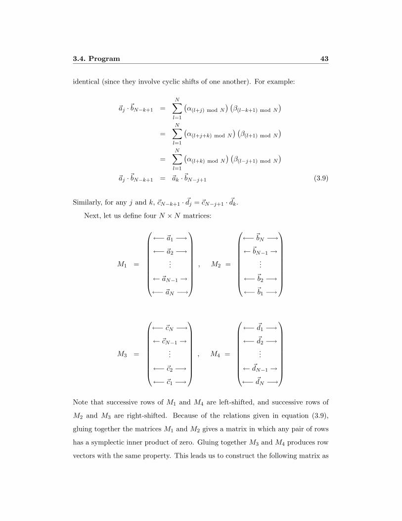
3.4. Program 43
identical (since they involve cyclic shifts of one another). For example:
~aj ·~bN−k+1 =N∑
l=1
(α(l+j) mod N
) (β(l−k+1) mod N
)=
N∑l=1
(α(l+j+k) mod N
) (β(l+1) mod N
)=
N∑l=1
(α(l+k) mod N
) (β(l−j+1) mod N
)~aj ·~bN−k+1 = ~ak ·~bN−j+1 (3.9)
Similarly, for any j and k, ~cN−k+1 · ~dj = ~cN−j+1 · ~dk.
Next, let us define four N ×N matrices:
M1 =
←− ~a1 −→
←− ~a2 −→...
← ~aN−1 →
←− ~aN −→
, M2 =
←− ~bN −→
← ~bN−1 →...
←− ~b2 −→
←− ~b1 −→
M3 =
←− ~cN −→
← ~cN−1 →...
←− ~c2 −→
←− ~c1 −→
, M4 =
←− ~d1 −→
←− ~d2 −→...
← ~dN−1 →
←− ~dN −→
Note that successive rows of M1 and M4 are left-shifted, and successive rows of
M2 and M3 are right-shifted. Because of the relations given in equation (3.9),
gluing together the matrices M1 and M2 gives a matrix in which any pair of rows
has a symplectic inner product of zero. Gluing together M3 and M4 produces row
vectors with the same property. This leads us to construct the following matrix as

3.4. Program 44
a candidate for a basis of a symplectic lattice:
M =
M1 M2
M3 M4
(3.10)
We can enforce the constraints detM = 1 and MJMT = J (so that M is in
standard form, as described by equation (2.38) in Section 2.4) by choosing:
δ1
δ2...
δN
= M−11
M2
γ1
γ2
...
γN
+
1
0...
0
(3.11)
Any pair of rows of M then has an integral symplectic inner product. The rows
of M play two distinct roles. They form a set of basis vectors for a symplectic
self-dual lattice, and they also form a set of vectors ~vj satisfying equation (3.8),
which can be used to define the stabilizer code described by equation (3.2).
3.4.2 Algorithm
Consequently, we have the following program for searching for good self-dual sym-
plectic lattices:
1. Choose values for the 3N free parameters αj , βj , γj (e.g., initially at ran-
dom and later by perturbing some or all of the parameters away from the
currently best-known values).
2. Solve for δj by equation (3.11), and construct M as given by equation
(3.10). Consider the rows of M to be a basis for a lattice in R2N .
3. Compute a “reduced basis” for the lattice by the LLL algorithm [51]. This
algorithm has running time O(N12) and constructs a set of basis vectors that
are all at least 60 apart from one another.

3.4. Program 45
4. Find the (approximately) closest lattice point to the origin by exhausting
over adding and subtracting the reduced basis vectors.
5. If the minimum distance of the lattice is larger than in previous rounds, save
the values of the free parameters as the currently best-known. Return to
step one.
Computing the closest lattice point to the origin, given a basis for a lattice, is
in general a hard problem [3, 60]. We only perform an approximate computation
in our code, but we are fairly confident that it is accurate in practice, because our
program converged toward several lattices, such as D4 and E8 (see Section 3.5),
that are suspected to be optimal among all Euclidean lattices (not just among
symplectic lattices).
The initial values of the free parameters can be chosen more or less at ran-
dom. The only constraint is that the rows of M need to be linearly independent.
This program (which introduces perturbations away from the currently best-known
values during each round) is basically a simulated annealing process, which may
converge toward local maxima in the parameter space, so it is necessary to start at
various initial positions or provide ways to move away from these localized traps.
We found that instead of isolated global maxima, there appears to be a continuous
curve (or perhaps even multi-dimensional surface) in the parameter space that de-
fines symplectic lattices with the optimal minimum distance. This suggests that
there are further symmetries in our parameterization (probably of a rotational
nature) that are not being utilized. One explicit expression of such a symmetry
is exhibited for D4 in the next section, which was found with the help of Dave
Beckman [9].

3.5. Results 46
Table 3.1: Best-known symplectic self-dual lattices
lattice (min. dist.)4 min. dist.
A243 1.075
D4 2 1.189
F6125 1.245
E8 4 1.414
D10 4 1.414
K12163 1.520
3.5 Results
The symplectic self-dual lattices with largest known minimum distances are given
in Table 3.1 (see also Table A.3). All of the lattice notations follow that of Conway
and Sloane [21], except for the six-dimensional lattice F6, which belongs to Bavard’s
family of lattices presented in appendix A.
These best-known symplectic self-dual lattices correspond to optimal Euclidean
lattices, except in dimensions 6 and 10, where E6 has minimum distance (643 )
112 ≈
1.290 and P10c has minimum distance (40)110 ≈ 1.446 [21]. Furthermore, it has
been claimed that the Barnes-Wall lattice Λ16 and the Leech lattice Λ24, which are
presumed to be optimal among lattices in dimensions 16 and 24 (with minimum
distances (2)34 ≈ 1.682 and 2, respectively), can be expressed as symplectic lattices
(see appendix of [17]). However, it remains an open question of finding a symplectic
basis for these lattices whose generator matrix has determinant 1. Nevertheless, we
conjecture that in dimensions that are a multiple of four, the optimal symplectic
self-dual lattices correspond to optimal Euclidean lattices. Rains has an argument
in favor of this in terms of searching for Hermitian lattices over Z[√−n ] (the ring
of integers extended by the number√−n) for various values of n [73]. It is also
interesting to note that the minimum distances of each of these optimal symplectic

3.5. Results 47
lattices is the fourth root of a rational number (see Table A.3 for more examples).
We can explicitly show a symplectic self-dual form for most of these lattices.
Any two-dimensional self-dual lattice is automatically symplectic, because the sym-
plectic inner product of the two rows of its basis matrix is simply equal to its
determinant, which is one, by definition. We can represent A2 as:
A2 =1
4√
12
2 0
1√
3
For D4, we first will choose parameters to define a rotation matrix in O(4).
Let a, b ∈ (0, 1√2) with a 6= b, and let m,n ∈ ±1. We then define:
c = ±√
12− a2 , d = ±
√12− b2
e = − 1√2(am− bn) , f = − 1√
2(am+ bn)
g = − ac
e+ f− bd
e− f, h = − ac
e+ f+
bd
e− f
We can now express D4 in a rotated version of its standard basis:
D4 =1
4√
8
2 0 0 0
0 2 0 0
0 0 2 0
1 1 1 1
a a c c
b −b d −d
g h e f
h g f e
For F6, we simply provide a numerical basis found by our search program (along
with the reduced lattice given by the LLL algorithm [51]), which was found later

3.5. Results 48
to match the geometry of a member of Bavard’s family of lattices:
F6 =
0.83490 0.18699 −0.11630 0.64916 0.50833 0.35192
0.18699 −0.11630 0.83490 0.35192 0.64916 0.50833
−0.11630 0.83490 0.18699 0.50833 0.35192 0.64916
1.88321 0.46591 1.01245 3.06472 2.24387 1.39866
1.01245 1.88321 0.46591 2.24387 1.39866 3.06472
0.46591 1.01245 1.88321 1.39866 3.06472 2.24387
F ′6 =
0.83490 0.18699 −0.11630 0.64916 0.50833 0.35192
0.18699 −0.11630 0.83490 0.35192 0.64916 0.50833
−0.11630 0.83490 0.18699 0.50833 0.35192 0.64916
−0.16057 0.32454 −0.42474 1.06257 −0.07111 −0.32183
0.22317 0.14273 −0.62666 0.22613 −0.46266 0.90616
0.02124 0.52646 −0.80847 −0.16542 0.76533 0.06972
(F ′6)(F
′6)
T =115
6 3 3 2 2 2
3 6 3 −1 −1 −1
3 3 6 2 2 2
2 −1 2 6 1 1
2 −1 2 1 6 1
2 −1 2 1 1 6
The actual parameters output by our program are reported to around 14 signifi-
cant digits, and they agree with the Euclidean inner products reported above to
better than 1 part in 109. Similar convergence was observed for the other lat-
tices (although somewhat less in higher dimensions, due to the greatly increased
running time required to search in the larger parameter spaces).
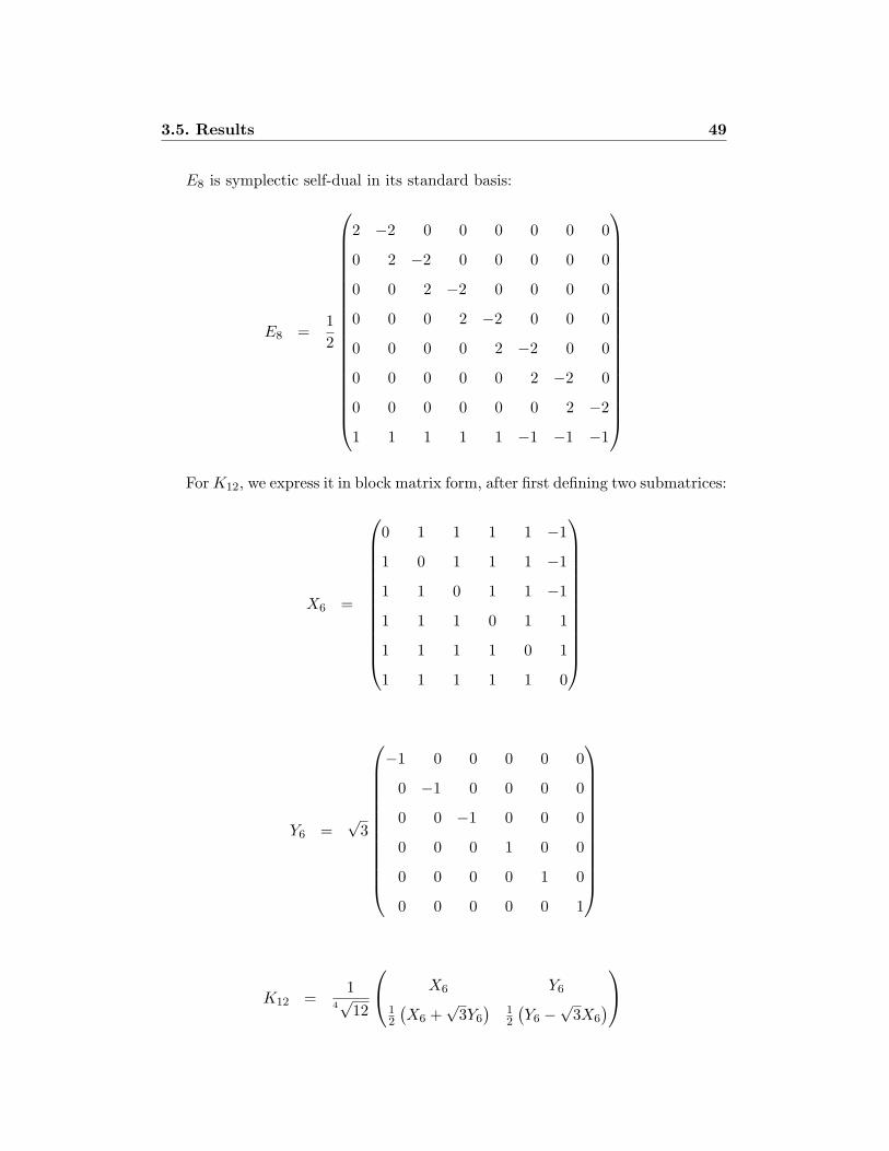
3.5. Results 49
E8 is symplectic self-dual in its standard basis:
E8 =12
2 −2 0 0 0 0 0 0
0 2 −2 0 0 0 0 0
0 0 2 −2 0 0 0 0
0 0 0 2 −2 0 0 0
0 0 0 0 2 −2 0 0
0 0 0 0 0 2 −2 0
0 0 0 0 0 0 2 −2
1 1 1 1 1 −1 −1 −1
ForK12, we express it in block matrix form, after first defining two submatrices:
X6 =
0 1 1 1 1 −1
1 0 1 1 1 −1
1 1 0 1 1 −1
1 1 1 0 1 1
1 1 1 1 0 1
1 1 1 1 1 0
Y6 =√
3
−1 0 0 0 0 0
0 −1 0 0 0 0
0 0 −1 0 0 0
0 0 0 1 0 0
0 0 0 0 1 0
0 0 0 0 0 1
K12 =1
4√
12
X6 Y6
12
(X6 +
√3Y6
)12
(Y6 −
√3X6
)

3.6. Error models 50
3.6 Error models
Given a 2N -dimensional symplectic self-dual lattice described by basis matrix M ,
we can construct a stabilizer code encoding N qudits (d-dimensional quantum
systems) into N oscillators. The stabilizer lattice, with basis operators Sj given
by equation (3.2), is simply√dM , and the normalizer lattice, with basis operators
Sj given by equation (3.3), is simply 1√dM .
Let A = MJMT be the Gram matrix of M , where J =(
0 IN−IN 0
), and
let ω = exp 2πi/d be a dth root of unity. We can compute the commutation
relations of the normalizer basis operators:
SjSk = ωAjk SkSj (3.12)
We can then assign any set of independent logical operators (which act nontrivially
on the N encoded qudits) to the normalizer basis operators Sj , as long as they obey
the above commutation relations. We will restrict ourselves to tensor products of
generalized Pauli operators (of the form ZaXb, for some integers a, b).
If the probability of a shift in phase space is governed by a Gaussian distribu-
tion (as in the Gaussian quantum channel, which was described in Section 2.3),
we may be able to consider just the nearest (first shell) lattice points about the
origin in the normalizer lattice, in order to identify what errors typically occur
when error correction fails. In the following subsections, we examine some logi-
cal operator assignments to the smallest normalizer basis elements and consider
how the Gaussian channel acting on the oscillators is transformed into an effective
channel on the encoded qudits.
3.6.1 The square lattice Z2
As comparison, we first consider the simplest encoding of a qudit into an oscil-
lator (see Section VIII of [38] for more detailed calculations). The Z2 lattice is

3.6. Error models 51
rectangular with minimum distance 1 between lattice points. A basis for the lat-
tice is given by the rows of M = ( 1 00 1 ), and its Gram matrix (which contains the
symplectic inner product relations) is A = MJMT = J =(
0 1−1 0
). Note that
S1 = expi√
2πdp
and S2 = expi√
2πdq
. See Figure 3.1 for a picture of this
lattice.
We can associate with S1 and S2 any pair of Pauli operators acting on a qudit
that obey S1S2 = ωS2S1. For example, let S1 = Z and let S2 = X. The nearest
points to the origin in the Z2 normalizer lattice are then associated with Z, X, Z−1,
and X−1. Under the Gaussian quantum channel, the probability of kicks in phase
space with large magnitude is greatly suppressed. If typical shifts have a magnitude
less than half the minimum distance of the normalizer lattice (which is 1/√d for
Z2), then on the rare occasions that error correction fails due to an atypically
large shift, it is most likely that the resulting logical error will be one of these four
(which are equally likely to occur).
Let pfail be the probability that there is a kick in the oscillator’s phase space
that extends beyond the Voronoi cell about the origin (which for Z2’s normalizer
lattice is a square of side length 1/√d centered about the origin). Effectively, the
Gaussian quantum channel is then converted into a Pauli channel described by
ρ −→ (1− pfail)ρ+(pfail
4
) (ZρZ−1 + Z−1ρZ + XρX−1 + X−1ρX
). (3.13)
For qubits (d = 2), this is just the binary independent Pauli channel (if we ignore
higher order terms in pfail). The next few closest points in the normalizer lattice
could also be included, but this would only be needed for noisier Gaussian channels
(or for larger d). (These additional error terms are included when we calculate
achievable rates in the regime of high noise.)
3.6.2 The hexagonal lattice A2
The A2 lattice corresponds to the densest packing of spheres in two dimensions. As
seen previously, we can express its basis vectors as the rows of M = 14√
12
(2 01√
3
),

3.6. Error models 52
S1
2S
Figure 3.1: The normalizer lattice of the Z2 encoding. The black circles denote the
lattice points. The stabilizer lattice is a sublattice of the normalizer lattice (shown
here with d = 2). The Voronoi cells of the stabilizer lattice points are indicated
by dashed lines. The normalizer basis elements S1 and S2 are drawn in blue.

3.6. Error models 53
and like Z2, its Gram matrix is A = MJMT = J =(
0 1−1 0
). See Figure 3.2 for a
picture of this lattice.
The Voronoi cell of the normalizer lattice of A2 is a hexagon, and there are
six points of minimum distance from any lattice point. If a sphere (circle) with
diameter 4√
12 was centered about every lattice point of A2, its kissing number
would be six. Since S1S2 = ωS2S1, we can choose S1 = Z and S2 = X. The
six points closest to the origin are then represented by (in counterclockwise order)
Z, X, Z−1X, Z−1, X−1, and ZX−1. If we are encoding qubits (d = 2), this is
simply the depolarizing channel, with equiprobable X, Y , and Z errors. For larger
d, the effective channel is a Pauli channel with six distinct and equiprobable errors
(other than the identity).
3.6.3 The checkerboard lattice D4
For the single oscillator encodings (with two-dimensional lattices), the effective
error channel is unique up to symmetries in our choice of assigning the logical
operators S1 and S2. However, for D4 and higher dimensions, we will find that
there are distinct choices.
The D4 lattice has a kissing number of 24. (If the lattice points are centers of
spheres with diameter 4√
2, then 24 spheres touch each sphere.) We can choose a
basis M for the D4 lattice such that its Gram matrix is A = MJMT = J . This
tells us that S1S3 = ωS3S1 and S2S4 = ωS4S2, while all other pairings of basis
normalizer operators commute.
We exhaustively find that there are 17312 ways consistent with the commuta-
tion relations to map 2-qudit Pauli operators (of the form (ZaXb)⊗ (ZcXd) with
a, b, c, d ∈ −1, 0, 1) to these basis elements. (If we restrict to qubits, there are
720 distinct mappings.) Some of the error operators are correlated errors on the
two encoded qudits, and others act nontrivially on just one of the qudits. If we
ignore any correlations between the qudits (which can only decrease the achiev-
able rate by throwing away some knowledge of the errors), we could consider what
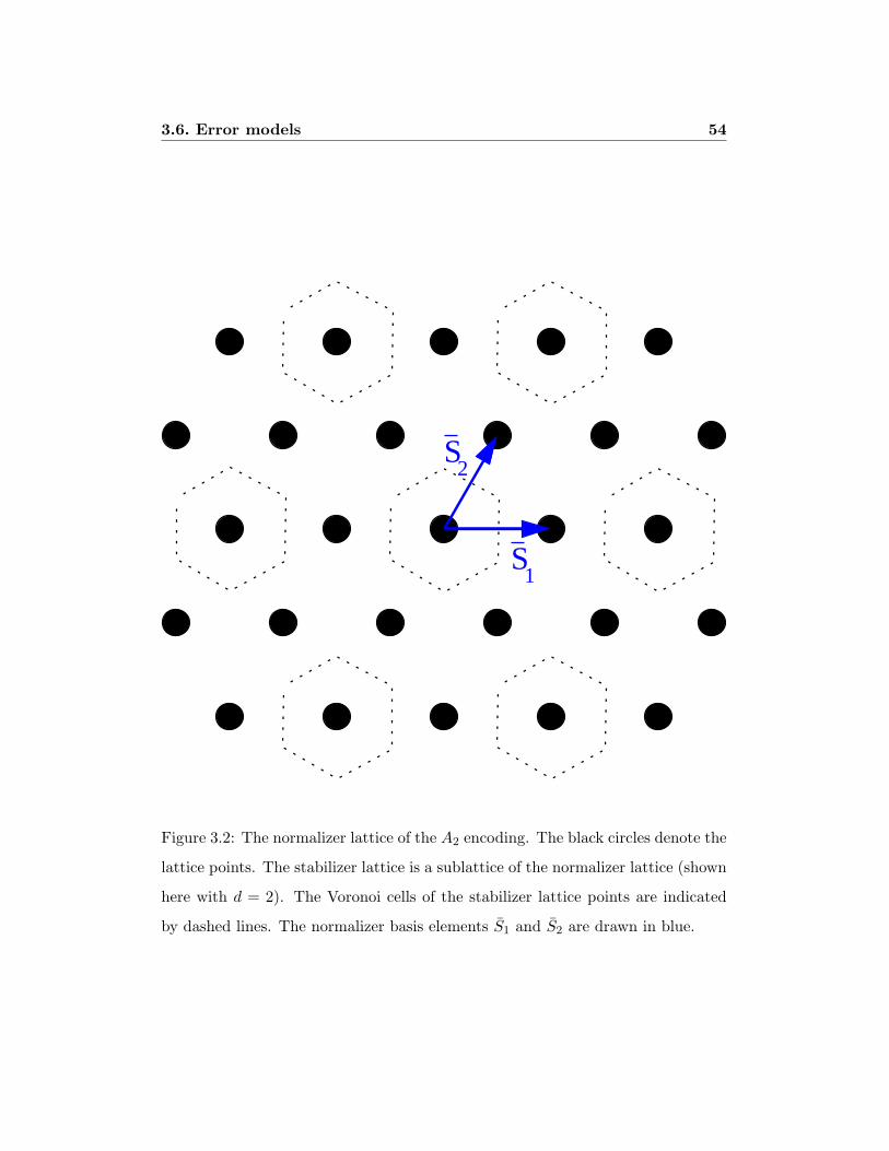
3.6. Error models 54
S1
S2
Figure 3.2: The normalizer lattice of the A2 encoding. The black circles denote the
lattice points. The stabilizer lattice is a sublattice of the normalizer lattice (shown
here with d = 2). The Voronoi cells of the stabilizer lattice points are indicated
by dashed lines. The normalizer basis elements S1 and S2 are drawn in blue.
3.6. Error models 55
the effective channel is on each encoded qudit separately. When we examine the
resulting logical errors of the 24 nearest points in the normalizer lattice, we find
that there are only two distinct effective channels, once symmetries are accounted
for.
As an example with qubits (d = 2), we could choose S1 = ZAZB, S2 = ZAIB,
S3 = IAXB, S4 = XAXB (acting on qubits A and B). We then find that the
logical operators for the normalizer lattice points in the first shell are IAXB,
IAZB, XAXB, XAZB, YAIB, YAXB, YAYB, YAZB, ZAIB, ZAXB, ZAYB, ZAZB.
Looking at each qubit separately, we would expect that when error correction fails,
the effective channel is a pair of Pauli channels with the following probabilities:
qubit A : pI =(
1− 56pfail
), pX =
16pfail, pY =
13pfail, pZ =
13pfail
qubit B : pI =(
1− 56pfail
), pX =
13pfail, pY =
16pfail, pZ =
13pfail
Or, we could assign instead S1 = ZAIB, S2 = IAZB, S3 = XAIB, S4 = IAXB,
in which case the most likely errors become IAXB, IAYB, IAZB, XAIB, XAXB,
XAYB, YAIB, YAYB, YAZB, ZAIB, ZAXB, ZAZB. This leads to effective error
channels described by:
qubit A : pI =(
1− 34pfail
), pX =
14pfail, pY =
14pfail, pZ =
14pfail
qubit B : pI =(
1− 34pfail
), pX =
14pfail, pY =
14pfail, pZ =
14pfail
It is worth noting that for any value of pfail, the Shannon entropy of the set of
probabilities in the first assignment is always higher than in the second, so we can
achieve a higher rate with the latter choice.
When encoding qudits with d > 2, the best effective channel is similar to
the depolarizing channel. For example, with S1 = ZAIB, S2 = IAZB, S3 = XAIB,
S4 = IAXB, the resulting error probability vector for each qudit channel is (1− 34p,
18p,
18p,
18p,
18p,
18p,
18p) with p = pfail.

3.6. Error models 56
3.6.4 Bavard’s symplectic lattice F6
Using the expression found by our program for a basis of F6, its Gram matrix is
A = MJMT =
0 0 0 1 0 0
0 0 0 0 1 0
0 0 0 0 0 1
−1 0 0 0 −1 0
0 −1 0 1 0 1
0 0 −1 1 −1 0
.
There are too many assignments to exhaust over to find the optimal effective qudit
error channels, as we did for D4. (We generated close to a million unique assign-
ments that are consistent with these commutation relations, but we estimate that
this was only about 1% of the possibilities, even with the Pauli operators lim-
ited to the form (ZaXb) with a, b ∈ −1, 0, 1.) However, we will present the
best effective channel (in terms of lowest Shannon entropy of its probability vec-
tors) that we found. Suppose we set S1 = XAXB IC , S2 = (ZX)A(Z−1X−1)BXC ,
S3 = (Z−1X−1)AZB(ZX)C , S4 = (Z−1X−1)AIB IC , S5 = XAIBXC , and S6 =
IAXB(Z−1X−1)C . The resulting logical errors associated with the nearest 44
points produce three effective Pauli channels each with error probability vector
(1− 3044p,
644p,
644p,
644p,
644p,
344p,
344p) with p = pfail.
3.6.5 The exceptional Lie algebra lattice E8
There is an incredibly large set of logical operator assignments consistent with
required commutation relations for the E8, and we could only sample a small
fraction of these. The E8 lattice has a kissing number of 240. The best effective
error channel we could find (when examining each qudit separately) has an error
probability vector (1 − 168240p,
27240p,
27240p,
27240p,
27240p,
27240p,
27240p,
1240p,
1240p,
1240p,
1240p,
1240p,
1240p) with p = pfail.

3.7. Achievable rates 57
p_fail
1.
.1
.1e-1
.1e-2
.1e-3
sigma
0.450.40.350.30.250.2
Figure 3.3: Failure probability of A2, D4, F6, and E8 lattice encodings over the
Gaussian channel. Sigma along the horizontal axis denotes the standard deviation
of the magnitude of the kicks by the channel in each oscillator’s phase space. The
red, blue, green, and magenta lines are respectively the plots of the probability of
a phase space kick being outside the Voronoi cell of the A2, D4, F6, and E8 lattice
encodings of qubits.
3.7 Achievable rates
In order to compute achievable rates over the Gaussian quantum channel, we first
computed (via Monte Carlo simulations) the fidelities of the A2, D4, F6, and E8
lattice encodings of qubits (d = 2). We calculated the failure probability pfail of
these encodings by sampling how often a phase space shift governed by a Gaussian
distribution fell outside of the Voronoi cell of the origin. Our results are plotted in
FIgure 3.3 over a moderate range of the channel’s standard deviation σ. Note that
there is something like a threshold in this range, below which more sophisticated
encodings have much better fidelity, and above which the simplest encodings fail

3.7. Achievable rates 58
least often. The jaggedness of some of the curves for small values of pfail are
due to statistical noise in our samplings; we expect the real curves to be smooth
and convex. From these curves, we can compute the fidelity for encoding any
d-dimensional system simply by scaling σ by√
2d .
If we are concerned with sending quantum information faithfully over a Gaus-
sian quantum channel, we could consider implementing another level of encoding
on the logical qudits encoded in the oscillators, such as a random stabilizer code.
When the effective channel is a Pauli channel (which is the case for all of the
examples given in the previous section), we can make a random coding argument
that good stabilizer codes exist that achieve a rate (in faithful qubits sent per use
of the channel)
R = (log2 d) (1−Hd(~p)− ε) = (log2 d) (1− ε) +M∑
k=1
pk logd pk (3.14)
when the channel has M Pauli errors (including the identity), with corresponding
error probabilities pk (where Hd(~p) is the Shannon entropy of probability vector ~p
in terms of logarithms base d).
We have plotted the resulting achievable rates for the A2, D4, F6, and E8
lattice encodings, using the best found logical operator mappings, for several val-
ues of d in Figure 3.4. For each lattice encoding, we approximated the success
probability of error correction through Monte Carlo simulations of sampling the
Gaussian distribution over the corresponding normalizer lattice Voronoi cell. We
then selected the best found effective error channel described in the previous sec-
tion and computed an asymptotically achievable rate with random stabilizer codes
on the encoded qudits (in the limit of large block size).
For noisy Gaussian quantum channels (those with relatively large standard
deviation σ of oscillator kicks), the A2 encoding is almost always the best choice.
Although not shown on the plot, the A2 encoding beats out the Z2 encoding almost
everywhere (due to its larger minimum distance). The only exception is the region
around 0.5 < σ < 0.555, where Z2 achieves slightly higher rates, due to its simpler

3.7. Achievable rates 59
Rate
3
2.5
2
1.5
1
0.5
0
sigma
0.60.50.40.30.20.10
Figure 3.4: Achievable rates of A2, D4, F6, and E8 lattice encodings over the
Gaussian channel. Sigma along the horizontal axis denotes the standard deviation
of the magnitude of the kicks by the channel in each oscillator’s phase space. The
upper curve corresponds to the channel’s one-shot coherent information optimized
over Gaussian input states, which is conjectured to be additive and thus equal the
channel’s quantum capacity. The red, blue, green, and magenta lines below are
respectively plots of the achievable rates (in qubits per oscillator) for A2, D4, F6,
and E8 lattice encodings of qudits with dimensions 2, 3, 4, 5, 6, 7, and 8.

3.8. Conclusion 60
effective error channel. The ability to encode qudits over several oscillators only
provides a rate gain for less noisy channels. In particular, the E8 encoding appears
to win over the others for σ < 0.2. We know from Section 2.6 that in the regime
of small noise (small σ) there exist symplectic lattice encodings that allow us to
achieve rates matching the one-shot coherent information for Gaussian inputs,
which is the upper curve in the plot. However, for moderately noisy channels,
there is a discernable gap, on the order of one qubit. Perhaps there exist better
quantum error-correcting codes for this noisy regime.
3.8 Conclusion
We presented an algorithm to search for symplectic self-dual lattices with large
minimum distance, and expressed bases for the optimal symplectic self-dual lattices
in two, four, six, eight, and twelve dimensions, which provide explicit descriptions
of quantum error-correcting codes protecting against shifts in the phase space
of oscillators. We have found effective Pauli error channels when encoding qudits
into oscillators over the Gaussian quantum channel for several of these lattices. By
concatenating with random stabilizer codes, we computed achievable rates over the
channel.

61
Chapter 4
Accuracy threshold for toric codes
4.1 Abstract
We study the ±J random-plaquette Z2 gauge model (RPGM) in three spatial
dimensions, a three-dimensional analog of the two-dimensional ±J random-bond
Ising model (RBIM). The model is a pure Z2 gauge theory in which randomly cho-
sen plaquettes (occurring with concentration p) have couplings with the “wrong
sign” so that magnetic flux is energetically favored on these plaquettes. Excita-
tions of the model are one-dimensional “flux tubes” that terminate at “magnetic
monopoles” located inside lattice cubes that contain an odd number of wrong-sign
plaquettes. Electric confinement can be driven by thermal fluctuations of the flux
tubes, by the quenched background of magnetic monopoles, or by a combination of
the two. Like the RBIM, the RPGM has enhanced symmetry along a “Nishimori
line” in the p-T plane (where T is the temperature). The critical concentration
pc of wrong-sign plaquettes at the confinement-Higgs phase transition along the
Nishimori line can be identified with the accuracy threshold for robust storage of
quantum information using topological error-correcting codes: if qubit phase er-
rors, qubit bit-flip errors, and errors in the measurement of local check operators
all occur at rates below pc, then encoded quantum information can be protected
perfectly from damage in the limit of a large code block. Through Monte Carlo

4.2. Introduction 62
simulations, we measure pc0, the critical concentration along the T = 0 axis (a
lower bound on pc), finding pc0 = .0293± .0002. We also measure the critical con-
centration of antiferromagnetic bonds in the two-dimensional RBIM on the T = 0
axis, finding pc0 = .1031± .0001. Our value of pc0 is incompatible with the value of
pc = .1093± .0002 found in earlier numerical studies of the RBIM, in disagreement
with the conjecture that the phase boundary of the RBIM is vertical (parallel to
the T axis) below the Nishimori line. The model can be generalized to a rank-r
antisymmetric tensor field in d dimensions, in the presence of quenched disorder.
4.2 Introduction
Spin systems with quenched randomness have been extensively studied, leading to
valuable insights that apply to (for example) spin glass materials, quantum Hall
systems, associative memory, error-correcting codes, and combinatorial optimiza-
tion problems [59, 85, 65]. Gauge systems with quenched randomness, which have
received comparatively little attention, will be studied in this paper.
The gauge models we consider are intrinsically interesting because they provide
another class of simple systems with disorder-driven phase transitions. But our
investigation of these models has a more specific motivation connected to the
theory of quantum error correction.
In practice, coherent quantum states rapidly decohere due to uncontrollable
interactions with the environment. But in principle, if the quantum information
is cleverly encoded [76, 80], it can be stabilized and preserved using fault-tolerant
recovery protocols [77]. Kitaev [47, 48] proposed a particularly promising class of
quantum error-correcting codes (surface codes) in which the quantum processing
required for error recovery involves only local interactions among qubits arranged
in a two-dimensional block, and the protected information is associated with global
topological properties of the quantum state of the block. If the error rate is small,
then the topological properties of the code block are well protected, and error
4.2. Introduction 63
recovery succeeds with a probability that rapidly approaches one in the limit of
a large code block. But if the error rate is above a critical value, the accuracy
threshold, then quantum error correction is ineffective.
In [26], a precise connection was established between the accuracy threshold
achievable with surface codes and the confinement-Higgs transition in a three-
dimensional Z2 lattice gauge model with quenched randomness. The model has
two parameters: the temperature T and the concentration p of “wrong-sign” pla-
quettes. On wrong-sign plaquettes (which are analogous to antiferromagnetic
bonds in a spin system) it is energetically favorable for the Z2 magnetic flux to be
nontrivial. In the mapping between quantum error recovery and the gauge model,
the quenched fluctuations correspond to the actual errors introduced by the en-
vironment; these impose sites of frustration, magnetic monopoles, corresponding
to an “error syndrome” that can be measured by executing a suitable quantum
circuit. Thermally fluctuating magnetic flux tubes, which terminate at magnetic
monopoles, correspond to the ensemble of possible error patterns that could gen-
erate a particular error syndrome. (The temperature T is tied to the strength p of
the quenched fluctuations through a Nishimori relation [63].) When the disorder is
weak and the temperature low (corresponding to a small error rate), the system is
in a magnetically ordered Higgs phase. In the surface code, magnetic order means
that all likely error patterns that might have produced the observed error syn-
drome are topologically equivalent, so that the topologically encoded information
resists damage. But at a critical value pc of the disorder strength (and a tem-
perature determined by Nishimori’s relation), magnetic flux tubes condense and
the system enters the magnetically disordered confinement phase. In the surface
code, magnetic disorder means that the error syndrome cannot point to likely error
patterns belonging to a unique topological class; therefore topologically encoded
information is vulnerable to damage.
Although the code block is two-dimensional, the gauge model is three dimen-
sional because one dimension represents time. Time enters the analysis of recovery
because measurements of the error syndrome might themselves be faulty; there-

4.2. Introduction 64
fore measurements must be repeated on many successive time slices if they are to
provide reliable information about the errors that have afflicted the code block.
If qubit phase errors, qubit bit-flip errors, and errors in the measurement of local
check operators all occur at rates below pc, then encoded quantum information
can be protected perfectly from damage in the limit of a large code block. As we
consider more and more reliable measurements of the syndrome, the correspond-
ing three-dimensional gauge model becomes more and more anisotropic, reducing
in the limit of perfect measurements to the two-dimensional random-bond Ising
model.
The numerical value pc of the accuracy threshold is of considerable interest,
since it characterizes how reliably quantum hardware must perform in order for a
quantum memory to be robust. In the three-dimensional Z2 gauge model, pc is
the value of the wrong-sign plaquette concentration where the confinement-Higgs
boundary crosses the Nishimori line in the p-T plane. A lower bound on pc is
provided by the critical concentration pc0 on the T = 0 axis. In [26], an analytic
argument established that pc0 ≥ .0114. In this paper we report on a numerical
calculation that finds pc0 = .0293± .0002.
In the case where the error syndrome can be measured flawlessly, the crit-
ical error rate is given by the critical antiferromagnetic bond concentration on
the Nishimori line of the two-dimensional random-bond Ising model (RBIM). Nu-
merical calculations performed earlier by other authors [42, 58] have established
pc = .1093± .0002. According to a conjecture of Nishimori [64] and Kitatani [49],
this value of pc should agree with the critical bond concentration pc0 of the 2-D
RBIM on the T = 0 axis. The same reasoning that motivates this conjecture
for the RBIM indicates that pc = pc0 for the 3-D random-plaquette gauge model
(RPGM) as well. However, we have calculated pc0 in the 2-D RBIM numerically,
finding pc0 = .1031 ± .0001. Our value of pc0 agrees with an earlier numerical
calculation by Kawashima and Rieger [44], but disagrees with the conjecture that
pc = pc0.
In Section 4.3 we describe in more detail the properties of the 2-D RBIM
4.3. Models 65
and the 3-D RPGM, emphasizing the importance of the Nishimori line and the
inferences that can be made about the behavior of order parameters on this line.
Section 4.4 reviews the connection between the models and error recovery using
surface codes. Our numerical results for pc0 and for the critical exponent ν0 at
the T = 0 critical point are presented in Section 4.5. Section 4.6 summarizes our
conclusions.
4.3 Models
4.3.1 Random-bond Ising model
The two-dimensional ±J random-bond Ising model (RBIM) has a much studied
multicritical point at which both the temperature and the strength of quenched
disorder are nonzero. This model is an Ising spin system on a square lattice, with
a variable Si = ±1 residing at each lattice site i. Its Hamiltonian is
H = −J∑〈ij〉
τijSiSj , (4.1)
where J is the strength of the coupling between neighboring spins, and τij = ±1 is
a quenched random variable. (That is, τij depends on what sample of the system
is selected from a certain ensemble, but is not subject to thermal fluctuations.)
The τij ’s are independently and identically distributed, with the antiferromagnetic
choice τij = −1 (favoring that neighboring spins anti-align) occurring with prob-
ability p, and the ferromagnetic choice τij=+1 (favoring that neighboring spins
align) occurring with probability 1 − p. We refer to p as the concentration of
antiferromagnetic bonds, or simply the bond concentration.
The free energy F of the model at inverse temperature β, averaged over sam-
ples, is
[βF (K, τ)]Kp = −∑
τ
P (Kp, τ) lnZ(K, τ) (4.2)
4.3. Models 66
where
Z(K, τ) =∑S
exp
K∑〈ij〉
τijSiSj
(4.3)
is the partition function for sample τ (with K = βJ), and
P (Kp, τ) = (2 coshKp)−NB × exp
Kp
∑〈ij〉
τij
(4.4)
is the probability of the sample τ ; here
p
1− p= e−2Kp (4.5)
and NB is the number of bonds.
The partition function Z(K, τ) is invariant under the change of variable
Si → σiSi , τij → σiσjτij , (4.6)
where σi = ±1. Thus τ itself has no invariant meaning — samples τ and τ ′ that
differ by the change of variable have equivalent physics. The only invariant prop-
erty of τ that cannot be modified by such a change of variable is the distribution
of frustration that τ determines. If an odd number of the bonds contained in
a specified plaquette have τ = −1 then that plaquette is frustrated — an Ising
vortex resides at the plaquette. For purposes of visualization, we sometimes will
find it convenient to define the spin model on the dual lattice so that the spins
reside on plaquettes and the Ising vortices reside on sites. Then excited bonds
with τijSiSj = −1 form one-dimensional chains that terminate at the frustrated
sites.
Changes of variable define an equivalence relation on the set of 2NB τ con-
figurations: there are the 2NS elements of each equivalence class (the number of
changes of variable, where NS is the number of sites) and there are 2NS classes
(the number of configurations for the Ising vortices — note that NB = 2NS for

4.3. Models 67
a square lattice on the 2-torus, and that the number of plaquettes is NP = NS).
Denote a distribution of Ising vortices, or equivalently an equivalence class of τ ’s,
by η. The probability P (Kp, η) of η is found by summing P (Kp, τ) over all the
representatives of the class; hence
(2 coshKp)NBP (Kp, η) = (2 coshKp)NB∑τ∈η
P (Kp, τ)
=∑
σ
exp
Kp
∑〈ij〉
τijσiσj
= Z(Kp, η) . (4.7)
Apart from a normalization factor, the probability of a specified distribution of
frustration is given by the partition function of the model, but with K = βJ
replaced by Kp.
In this model, we can define an order parameter that distinguishes the ferro-
magnetic and paramagnetic phases. Let
m2(K,Kp) = lim|i−j|→∞
[〈SiSj〉K
]Kp
, (4.8)
where 〈·〉K denotes the average over thermal fluctuations, [·]Kp denotes the average
over samples, and |i − j| denotes the distance between site i and site j; then in
the ferromagnetic phase m2 > 0 and in the paramagnetic phase m2 = 0. But
the two-point correlation function 〈SiSj〉K is not invariant under the change of
variable eq. (4.6), so how should m2 be interpreted?
Following [26], denote by E the set of bonds that are antiferromagnetic (τij =
−1), denote by E′ the set of excited bonds with τijSiSj = −1, and denote by D
the set of bonds with SiSj = −1 (those whose neighboring spins anti-align) — see
Figure 4.1. Then D = E +E′ is the disjoint union of E and E′ (containing bonds
in E or E′ but not both). Furthermore, D contains an even number of the bonds
that meet at any given site; that is, D is a cycle, a chain of bonds that has no
boundary points. The quantity SiSj just measures whether a line connecting i and
j crosses D an even number (SiSj = 1) or an odd number (SiSj = −1) of times.
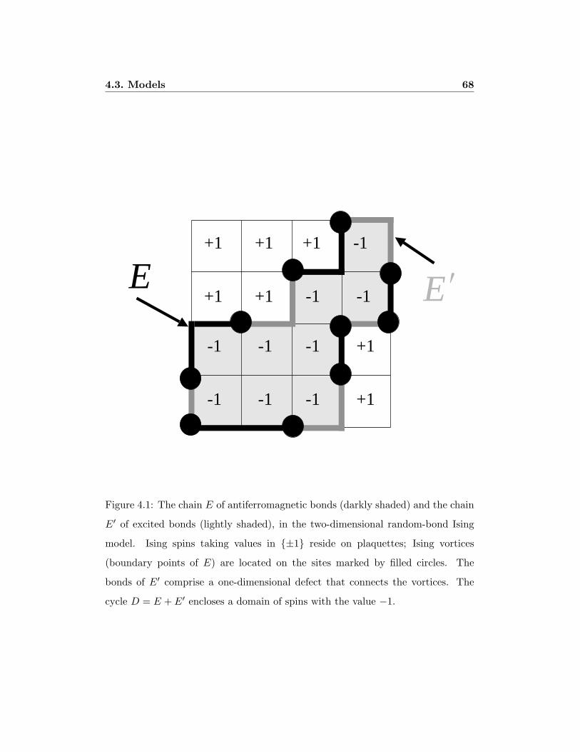
4.3. Models 68
-1
-1
+1
+1 +1 +1 -1
+1 -1 -1
-1 -1 +1
-1 -1 +1
E E′
Figure 4.1: The chain E of antiferromagnetic bonds (darkly shaded) and the chain
E′ of excited bonds (lightly shaded), in the two-dimensional random-bond Ising
model. Ising spins taking values in ±1 reside on plaquettes; Ising vortices
(boundary points of E) are located on the sites marked by filled circles. The
bonds of E′ comprise a one-dimensional defect that connects the vortices. The
cycle D = E + E′ encloses a domain of spins with the value −1.

4.3. Models 69
Now D consists of disjoint “domain walls” that form closed loops. If loops
that are arbitrarily large appear with appreciable weight in the thermal ensemble,
then the two-point function 〈SiSj〉K decays like exp(−|i− j|/ξ) — fluctuations far
from the sites i and j contribute to the correlation function. Thus the spins are
disordered and m2 = 0. But if large loops occur only with negligible probability,
then only fluctuations localized near i and j contribute significantly; the spin
correlation persists at large distances and m2 > 0. Thus, the order parameter
probes whether the chain E′ of excited bonds can wander far from the chain E
of ferromagnetic bonds; that is, whether D = E + E′ contains arbitrarily large
connected closed loops, for typical thermal fluctuations and typical samples.
Nishimori [63] observed that the random-bond Ising model has enhanced sym-
metry properties along a line in the p-T plane (the Nishimori line) defined by
K = Kp or exp(−2βJ) = p/(1−p). In this case, the antiferromagnetic bond chain
E and the excited bond chain E′ are generated by sampling the same probability
distribution, subject to the constraint that both chains have the same boundary
points. This feature is preserved by renormalization group transformations, so that
renormalization group flow preserves Nishimori’s line [28]. The Nishimori point
(pc, Tc) where the Nishimori line crosses the ferromagnetic-paramagnetic phase
boundary, is a renormalization group fixed point, the model’s multicritical point.
When the temperature T is above the Nishimori line, excited bonds have a
higher concentration than antiferromagnetic bonds, so we may say that thermal
fluctuations play a more important role than quenched randomness in disordering
the spins. When T is below the Nishimori line, antiferromagnetic bonds are more
common than excited bonds, and the quenched randomness dominates over ther-
mal fluctuations. Right on the Nishimori line, the effects of thermal fluctuations
and quenched randomness are in balance [66].
By invoking the change of variable eq. (4.6), various properties of the model
on the Nishimori line can be derived [65, 63]. For example, the internal energy

4.3. Models 70
density (or “average bond”) can be computed analytically,
[τij〈SiSj〉Kp ]Kp = 1− 2p , (4.9)
where i and j are neighboring sites; averaged over thermal fluctuations and sam-
ples, the concentration of excited bonds is p as one would expect (and the internal
energy has no singularity at the Nishimori point). Furthermore, after averaging
over disorder, the (2m− 1)st power of the k-spin correlator has the same value as
the (2m)th power, for any positive integer m:
[〈Si1Si2 · · ·Sik〉
2m−1Kp
]Kp
=[〈Si1Si2 · · ·Sik〉
2mKp
]Kp
. (4.10)
It follows in particular that the spin-glass order parameter
q2(Kp,Kp) ≡ lim|i−j|→∞
[〈SiSj〉2Kp
]Kp
(4.11)
coincides with the ferromagnetic order parameter m2(Kp,Kp) along the Nishimori
line, reflecting the property that thermal fluctuations and quenched randomness
have equal strength on this line.
Comparing eq. (4.2) and (4.7), we see that for K = Kp the free energy of the
model coincides with the Shannon entropy of the distribution of vortices, apart
from a nonsingular additive term:
[βF (Kp, τ)]Kp
= −∑
η
P (Kp, η) lnP (Kp, η)−NB ln (2 coshKp) . (4.12)
Since the free energy is singular at the Nishimori point (pc, Tc), it follows that the
Shannon entropy of frustration (which does not depend on the temperature) is
singular at p = pc [64]. This property led Nishimori to suggest that the boundary
between the ferromagnetic and paramagnetic phases occurs at p = pc at sufficiently
low temperature, and thus that the phase boundary is vertical in the p-T plane be-

4.3. Models 71
T
p
ordered
disordered
pc
“NishimoriLine”
pc0
T
p
ordered
disordered
pc
“NishimoriLine”
(a) (b)
Figure 4.2: The phase diagram of the random-bond Ising model (shown schem-
atically), with the temperature T on the vertical axis and the concentration p of
antiferromagnetic bonds on the horizontal axis. The solid line is the boundary be-
tween the ferromagnetic (ordered) phase and the paramagnetic (disordered) phase.
The dotted line is the Nishimori line e−2βJ = p/(1 − p), which crosses the phase
boundary at the Nishimori point (the heavy black dot). It has been conjectured,
but not proven, that the phase boundary from the Nishimori point to the p-axis is
vertical, as in (a). The numerics reported in Section 4.4 favor the reentrant phase
diagram shown in (b). The deviation of the critical bond concentration pc on the
Nishimori line from the critical bond concentration pc0 on the T = 0 axis has been
exaggerated in (b) for clarity.

4.3. Models 72
low the Nishimori point, as in Figure 4.2a. Later, Kitatani [49] arrived at the same
conclusion by a different route, showing that the verticality of the phase boundary
follows from an “appropriate condition.” These arguments, while suggestive, do
not seem compelling to us. There is no known rigorous justification for Kitatani’s
condition, and no rigorous reason why the ferro-para boundary must coincide with
the singularity in the entropy of frustration, even at low temperature. Hence we
regard the issue of the verticality of the phase boundary as still unsettled. Nishi-
mori did argue convincingly that the phase boundary cannot extend to any value
of p greater than pc [63], and Le Doussal and Harris argued that the tangent to
the phase boundary is vertical at the Nishimori point [28], but these results leave
open the possibility of a “reentrant” boundary that slopes back toward the T axis
below the Nishimori point, as in Figure 4.2b.
The RBIM can also be defined in d dimensions. Much of the above discussion
still applies, with minor modifications. Consider, for example, d = 3. On the dual
lattice, spins reside on lattice cubes and the bonds become plaquettes shared by
two neighboring cubes. The set of antiferromagnetic bonds E is dual to a two-
dimensional surface, and its boundary ∂E consists of one-dimensional loops — the
Ising strings where the spins are frustrated. The set of excited bonds E′ is dual to
another two-dimensional surface that is also bounded by the Ising strings: ∂E′ =
∂E. The spins are disordered if the two-cycle D = E+E′ contains arbitrarily large
closed connected surfaces for typical thermal fluctuations and typical samples.
Similarly, in d dimensions, frustration is localized on closed surfaces of dimension
d − 2, and the thermally fluctuating defects are dimension-(d − 1) surfaces that
terminate on the locus of frustration. For any d, the model has enhanced symmetry
along the Nishimori line K = Kp, where antiferromagnetic bonds and excited
bonds are drawn from the same probability distribution.
In the absence of quenched disorder, the two-dimensional Ising model is mapped
to itself by a duality relation that can be used to infer properties of the critical the-
ory. When quenched disorder is introduced, however, the two-dimensional random
bond Ising model is mapped under duality to a model with Boltzmann weights that
4.3. Models 73
are not positive definite [67], so that it is not easy to draw any firm conclusions.
4.3.2 Random-plaquette gauge model
In the d-dimensional RBIM, excitations have codimension 1 and terminate on a
closed surface of codimension 2. The Z2 random-plaquette gauge model (RPGM)
is defined in an entirely analogous manner, except that the excitations are objects
of codimension 2 (“magnetic flux tubes”) that terminate on codimension-3 objects
(“magnetic monopoles”).
More concretely, the variables of the model are U` = ±1 residing on each link
` of the lattice, and the Hamiltonian is
H = −J∑P
τPUP , (4.13)
where J is the coupling strength,
UP =∏`∈P
U` (4.14)
is the Z2-valued “magnetic flux” through the plaquette P , and τP = ±1 is a
quenched random variable. The τP ’s are independently and identically distributed,
with the “wrong-sign” choice τP = −1 (favoring nontrivial flux) occurring with
probability p, and the “right-sign” choice τP =+1 (favoring trivial flux) occurring
with probability 1−p. We refer to p as the concentration of wrong-sign plaquettes,
or simply the plaquette concentration.
The free energy F of the model at inverse temperature β, averaged over sam-
ples, is
[βF (K, τ)]Kp = −∑
τ
P (Kp, τ) lnZ(K, τ) (4.15)
where
Z(K, τ) =∑U
exp
(K∑P
τPUP
)(4.16)

4.3. Models 74
is the partition function for sample τ (with K = βJ), and
P (Kp, τ) = (2 coshKp)−NP × exp
(Kp
∑P
τP
)(4.17)
is the probability of the sample τ ; here
p
1− p= e−2Kp (4.18)
and NP is the number of plaquettes.
The partition function Z(K, τ) is invariant under the change of variable
U` → σ`U` , τP → σP τP , (4.19)
where σ` = ±1 and σP =∏
`∈P σ`. While τ itself has no invariant meaning,
τ determines a distribution of frustration that cannot be altered by a change of
variable. If an odd number of the plaquettes contained in a specified cube have
τ = −1 then that cube is frustrated — a Z2 magnetic monopole resides in the cube.
For purposes of visualization, we will sometimes find it convenient to define the
gauge model on the dual lattice so that the gauge variables U` reside on plaquettes,
the magnetic flux on bonds, and the magnetic monopoles on sites. Then excited
bonds with τPUP = −1 form one-dimensional strings that terminate at monopoles.
We can define an order parameter that distinguishes the Higgs (magnetically
ordered) phase and the confinement (magnetically disordered) phase. Consider
the Wilson loop operator associated with a closed loop C (on the original lattice,
not the dual lattice):
W (C) =∏`∈C
U` . (4.20)
and consider the behavior of the expectation value of W (C), averaged over thermal
fluctuations and over samples. In the Higgs phase, for a large loop C the Wilson

4.3. Models 75
loop operator decays exponentially with the perimeter of the loop,
[〈W (C)〉K ]Kp∼ exp [−µ · Perimeter(C)] , (4.21)
while in the confinement phase it decays exponentially with the area of the minimal
surface bounded by C,
[〈W (C)〉K ]Kp∼ exp [−κ ·Area(C)] . (4.22)
The interpretation is that on the dual lattice the wrong-sign plaquettes correspond
to a one-chain E bounded by magnetic monopoles, and the excited plaquettes
correspond to another one-chain E′ with the same boundary; hence D = E + E′
is a cycle, a sum of disjoint closed “flux tubes.” If arbitrarily large loops of flux
appear with appreciable weight in the thermal ensemble for typical samples, then
magnetic fluctuations spanning the entire surface bounded by C contribute to the
expectation value of W (C), and the area-law decay results. If large flux tubes are
suppressed, then only the fluctuations localized near the loop are important, and
the perimeter-law decay applies. Thus, the Wilson-loop order parameter probes
whether the chain E′ of excited plaquettes can wander far from the chain E of
wrong-sign plaquettes; that is, whether D = E + E′ contains arbitrarily large
connected closed loops.
The one-chain E bounded by the magnetic monopoles is analogous to a Z2-
valued Dirac string — the change of variable eq. (4.19) deforms the strings while
leaving invariant the boundary of E (the locations of the monopoles). One should
notice that these strings are not invisible to our Wilson loop operator; that is
W (C) is not invariant under the change of variable. It is possible to modify W (C)
to obtain an invariant object [4], but that would not be appropriate if the order
parameter is supposed to probe the extent to which the thermally fluctuating
defects (the excited plaquettes) depart from the quenched disorder (the Dirac
strings).

4.3. Models 76
Like the RBIM, the RPGM has enhanced symmetry on the Nishimori line
K = Kp, and the change of variable eq. (4.19) may be invoked to derive properties
of the model on this line. The Nishimori line is preserved by renormalization group
flow, and crosses the confinement-Higgs boundary at a multicritical point (pc, Tc).
The internal energy (or average plaquette) can be computed on this line,
[τP 〈UP 〉Kp
]Kp
= 1− 2p (4.23)
(excited plaquettes have concentration p) and for each positive integer m, the
(2m − 1)’st power of W(C) and the 2m’th power are equal when averaged over
samples, [〈W (C)〉2m−1
Kp
]Kp
=[〈W (C)〉2m
Kp
]Kp
. (4.24)
Furthermore, the free energy on the Nishimori line, apart from a nonsingular
additive term, is equal to the Shannon entropy of the distribution of magnetic
monopoles, so that the latter is singular at p = pc.
In principle, the RPGM could have what might be called a “gauge glass” phase.
In this phase, the Wilson loop, averaged over thermal and quenched fluctuations,
has area-law behavior,
[〈W (C)〉K ]Kp∼ exp [−κ ·Area(C)] , (4.25)
but the square of its thermal expectation value, averaged over quenched fluctua-
tions, has perimeter-law behavior:
[〈W (C)〉2K
]Kp∼ exp [−µ · Perimeter(C)] . (4.26)
This means that thermal fluctuations do not induce magnetic disorder for each
typical sample, but that the magnetic fluctuations are large when we compare
one sample to another. However, the identity eq. (4.24) shows that, along the
Nishimori line K = Kp, there can be no gauge glass phase. Since 〈W (C)〉 and
4.3. Models 77
〈W (C)〉2 have the same average over samples, both order parameters cross from
perimeter to area law at the same point on the Nishimori line. (Nishimori [63]
used the analogous argument to show that there is no spin glass behavior in the
RBIM along the Nishimori line.)
Another useful identity that can be derived using the change of variable is
[〈W (C)〉K ]Kp=[〈W (C)〉K〈W (C)〉Kp
]Kp
. (4.27)
Since −1 ≤W (C) ≤ 1, it follows that
∣∣∣ [〈W (C)〉K ]Kp
∣∣∣ ≤ [ ∣∣〈W (C)〉Kp
∣∣ ]Kp
. (4.28)
From this inequality, we may infer that if the point on the Nishimori line with
concentration p is in the confinement phase, then the point (p, T ) is in the confine-
ment phase for any temperature T . (Again, the reasoning is exactly analogous to
Nishimori’s argument for the RBIM [63].) Since there is no gauge-glass behavior
on the Nishimori line, if a point on the Nishimori line is in the confinement phase,
then 〈W (C)〉Kp already exhibits area-law decay before averaging over samples.
Therefore the right-hand side of eq. (4.28) shows area-law decay and so must the
left-hand side. We conclude that, as for the RBIM, the phase boundary of the
RPGM below the Nishimori line must either be vertical (parallel to the T axis as
in Figure 4.2a) or reentrant (tipping back toward the T axis as T decreases as in
Figure 4.2b).
4.3.3 Further generalizations
In d dimensions, the magnetic order parameter of the RBIM explores whether a
thermally excited chain E′ of codimension 1 (domain walls) deviates far from a
quenched codimension-1 chain E (antiferromagnetic bonds), where both E and
E′ have the same codimension-2 boundary (the Ising vortices). Similarly, the
RPGM can be defined in d dimensions, and its Wilson-loop order parameter probes
4.4. Accuracy threshold for quantum memory 78
whether a thermally excited chain E′ of codimension 2 (flux tubes) deviates far
from a quenched codimension-2 chain E (Dirac strings), where both E and E′ have
the same codimension-3 boundary (the magnetic monopoles).
This concept admits further generalizations. In d-dimensions, we may consider
the lattice theory of a “rank-r antisymmetric tensor field” with quenched disorder.
Then variables reside on the r-cells of the lattice, and the Hamiltonian is expressed
in terms of a field strength defined on (r + 1)-cells. The sign of the coupling is
determined by a random variable τ taking values ±1 on (r + 1)-cells; cells with
the “wrong sign” have concentration p. On the dual lattice, τ corresponds to a
codimension-(r+1) chain E, and the excited cells to a codimension-(r+1) chain E′,
where E and E′ are bounded by the same codimension-(r+2) chain of frustration.
An operator analogous to the Wilson loop can be defined that detects the flux
through the dimension-(r+ 1) “surface” bounded by a dimension-r “loop” C; this
operator serves as the order parameter for an order-disorder transition. The order
parameter probes whether the thermally fluctuating codimension-(r+ 1) chain E′
deviates far from the quenched codimension-(r + 1) chain E.
For any d and r, the model has enhanced symmetry on the Nishimori line,
where K = Kp. Properties of the model on this line can be derived, analogous to
those discussed above for the RBIM and the RPGM.
4.4 Accuracy threshold for quantum memory
How the RBIM and RPGM relate to the performance of topological quantum
memory was extensively discussed in [26]. Here we will just briefly reprise the
main ideas.
4.4.1 Toric codes
Quantum information can be protected from decoherence and other possible sour-
ces of error using quantum error-correcting codes [76, 80] and fault-tolerant error

4.4. Accuracy threshold for quantum memory 79
Z
Z
Z
Z
XX
XX
Figure 4.3: The check operators of the toric code. Each plaquette operator is a
tensor product of Z’s acting on the four links contained in the plaquette. Each
site operator is a tensor product of X’s acting on the four links that meet at the
site.
recovery protocols [77]. Topological codes (or surface codes) are designed so that
the quantum processing needed to control errors has especially nice locality prop-
erties [47, 48].
Specifically, consider a system of 2L2 qubits (a qubit is a two-level quantum
system), with each qubit residing at a link of an L× L square lattice drawn on a
two-dimensional torus. (Other examples of surface codes, including codes defined
on planar surfaces, are discussed in [26].) This system can encode two qubits of
quantum information that are well protected from noise if the error rate is low
enough. The two-qubit code space, where the protected information resides, can

4.4. Accuracy threshold for quantum memory 80
be characterized as a simultaneous eigenspace with eigenvalue one of a set of check
operators (or “stabilizer generators”); check operators are associated with each site
and with each elementary cell (or “plaquette”) of the lattice, as shown in Figure
4.3. We use the notation
I =
1 0
0 1
, X =
0 1
1 0
, Y =
0 −i
i 0
, Z =
1 0
0 −1
(4.29)
for the 2 × 2 identity and Pauli matrices. The check operator at site i acts non-
trivially on the four links that meet at the site; it is the tensor product
Xi = ⊗`3sX` (4.30)
acting on those four qubits, times the identity acting on the remaining qubits. The
check operator at plaquette P acts nontrivially on the four links contained in the
plaquette, as the tensor product
ZP = ⊗`∈PZ` , (4.31)
times the identity on the remaining links.
The check operators can be simultaneously diagonalized, and the toric code
is the space in which each check operator acts trivially. Because of the periodic
boundary conditions on the torus, the product of all L2 site operators or all L2
plaquette operators is the identity — each link operator occurs twice in the prod-
uct, and X2 = Z2 = I. There are no further relations among these operators;
therefore, there are 2 · (L2 − 1) independent check operators constraining the 2L2
qubits in the code block, and hence two encoded qubits (the code subspace is four
dimensional).
Since the check operators are spatially local, it is useful to think of a site or
plaquette where the check operator has the eigenvalue −1 as the position of a
localized excitation or “defect.” The code space contains states with no defects,

4.4. Accuracy threshold for quantum memory 81
which are analogous to vacuum states of a Z2 gauge theory on the torus: ZP = 1
means that there is no Z2 magnetic flux at plaquette P , and Xi = 1 means that
there is no Z2 electric charge at site i. (This Z2 gauge theory on the two-torus
should not be confused with the three-dimensional Z2 gauge theory, described in
Section 4.4.3, that arises in the analysis of the efficacy of error correction!)
Consider applying to the vacuum state an operator that is a tensor product
of Pauli matrices Z` acting on each of a set of links forming a connected chain
`. This operator creates isolated site defects at the ends of the chain. Similarly,
if we apply to the vacuum a tensor product of Pauli matrices X` acting on a
connected chain of the dual lattice, isolated plaquette defects are created at the
ends of the chain, as in Figure 4.4. A general “Pauli operator” (tensor product of
Pauli matrices) can be expressed as tensor product of X`’s and I`’s times a tensor
products of Z`’s and I`’s; this operator preserves the code space if and only if the
links acted upon by Z’s comprise a cycle of the lattice (a chain with no boundary)
and the links acted upon by X’s comprise a cycle of the dual lattice.
Cycles on the torus are of two types. A homologically trivial cycle is the bound-
ary of a region that can be tiled by plaquettes. A product of Z’s acting on the
links of the cycle can be expressed as a product of the enclosed plaquette opera-
tors, which acts trivially on the code space. A homologically nontrivial cycle wraps
around the torus and is not the boundary of anything. A product of Z’s acting
on the links of the cycle preserves the code space, but acts nontrivially on the
encoded quantum information. Associated with the two fundamental nontrivial
cycles of the torus are encoded operations Z1 and Z2 acting on the two encoded
qubits. Similarly, associated with the two dual cycles of the dual lattice are the
corresponding encoded operations X1 and X2, as shown in Figure 4.5.
A general error acting on the code block can be expanded in terms of Pauli
operators. Therefore, we can characterize the efficacy of error correction by con-
sidering how well we can protect the encoded state against Pauli operator errors.
With the toric code, X errors (bit flips) and Z errors (phase flips) can be corrected
independently; this suffices to protect against general Pauli errors, since a Y error

4.4. Accuracy threshold for quantum memory 82
Figure 4.4: Site defects and plaquette defects in the toric code. Applied to the
code space, Z’s acting on a connected chain of links (darkly shaded) create site
defects (electric charges) at the ends of the chain. Similarly, X’s applied to a
connected chain of dual links (lightly shaded) create plaquette defects (magnetic
fluxes) at the ends of the chain.

4.4. Accuracy threshold for quantum memory 83
(a) (b)
1Z
1X2Z
2X
Figure 4.5: Basis for the operators that act on the two encoded qubits of the
toric code. (a) The encoded Z1 is a tensor product of Z’s acting on lattice links
comprising a cycle of the torus, and the encoded X1 is a tensor product of X’s
acting on dual links comprising the complementary cycle. (b) Z2 and X2 are
defined similarly.

4.4. Accuracy threshold for quantum memory 84
is just a bit flip and a phase flip acting on the same qubit. We may therefore
confine our attention to Z errors; the X errors may be dealt with in essentially
the same way, but with the lattice replaced by its dual.
4.4.2 Perfect measurements and the random-bond Ising model
To be concrete, suppose that the Z errors are independently and identically dis-
tributed, occurring with probability p on each qubit. Noise produces an error chain
E, a set of qubits acted upon by Z. To diagnose the errors, the code’s local check
operators are measured at each lattice site, the measurement outcomes providing a
“syndrome” that we may use to diagnose errors. However, the syndrome is highly
ambiguous. It does not completely characterize where the errors occurred; rather
it only indicates whether the number of damaged qubits adjacent to each site is
even or odd. That is, the measurement determines the boundary ∂E of the error
chain E.
To recover from the damage, we choose a recovery chain E′ that has the same
boundary as the measured boundary of E, and apply Z to all the qubits of E′.
Since ∂E = ∂E′, the chain D = E + E′ is a cycle with ∂D = 0. Now, if D
is homologically trivial, then the recovery successfully protects the two encoded
qubits — the effect of the errors together with the recovery step is just to apply a
product of check operators, which has trivial action on the code space. But if D is
homologically nontrivial, then recovery fails — the encoded quantum information
suffers an error.
Error recovery succeeds, then, if we can guess the homology class of the ran-
domly generated chain E, knowing only its boundary ∂E — we succeed if our guess
E′ = E+D differs from E by a homologically trivial cycle D. If the error rate p is
below a certain critical value pc called the accuracy threshold, it is possible to guess
correctly, with a probability of failure that approaches zero for a sufficiently large
linear size L of the lattice. But if p is above pc, the failure probability approaches a
nonzero constant as L→∞. The numerical value of pc is of considerable interest,

4.4. Accuracy threshold for quantum memory 85
since it characterizes how reliably quantum hardware must perform for a quantum
memory to be robust.
Let prob(E) denote the probability that the error chain is E, and let prob[(E+
D)|E] denote the normalized conditional probability for error chains E′ = E +D
that have the same boundary as E. Then, the probability of error per qubit lies
below threshold if and only if, in the limit L→∞,
∑E
prob(E) ·∑
D nontrivial
prob[(E +D)|E] = 0 . (4.32)
Eq. (4.32) says that error chains that differ from the actual error chain by a
homologically nontrivial cycle have probability zero. Therefore, the outcome of
the measurement of the check operators is sure to point to the correct homology
class, in the limit of an arbitrarily large code block.
This criterion is identical to the criterion for long-range order in the two-
dimensional RBIM, along the Nishimori line. The error chain E can be identified
with the chain of antiferromagnetic bonds of a sample, bounded by Ising vortices
that are pinned down by the measurement of the local check operators. The
ensemble of all the chains E′ with a specified boundary can be interpreted as
a thermal ensemble. If the temperature T and the error rate p obey Nishimori’s
relation, then the chain E′ and the chain E have the same bond concentration.
At low temperature along the Nishimori line, the cycle D = E + E′ contains
no large connected loops for typical samples and typical thermal fluctuations —
the spin system is magnetically ordered and error recovery succeeds with high
probability. But at higher temperature, the quenched chain E and the thermal
chain E′ fluctuate more vigorously. At the Nishimori point, D contains loops
that “condense,” disordering the spins and compromising the effectiveness of error
correction. Thus, the critical concentration pc at the Nishimori point of the two-
dimensional RBIM coincides with the accuracy threshold for quantum memory
using toric codes (where pc is the largest acceptable probability for either an X
error or a Z error).

4.4. Accuracy threshold for quantum memory 86
The optimal recovery procedure is to choose a recovery chain E′ that belongs to
the most likely homology class, given the known boundary of the chain ∂E′ = ∂E.
For p < pc, the probability distribution has support on a single class in the limit
L → ∞, and the optimal recovery procedure is sure to succeed. In the language
of the RBIM, for a given sample with antiferromagnetic chain E, a chain E′ of
excited bonds can be classified according to the homology class to which the cycle
D = E+E′ belongs, and a free energy can be defined for each homology class. For
p < pc along the Nishimori line, the trivial homology class has lowest free energy,
and the free energy cost of choosing a different class diverges as L→∞.
An alternative recovery procedure is to choose the single most likely recovery
chain E′, rather than a chain that belongs to the most likely class. In the language
of the RBIM, this most likely recovery chain E′ for a given sample is the set of
excited links that minimizes energy rather than free energy. This energy mini-
mization procedure is sure to succeed if the error rate is p < pc0, where pc0 is the
critical bond concentration of the RBIM at T = 0. Since minimizing energy rather
than free energy need not be optimal, we see that pc0 ≤ pc. However, the energy
minimization procedure has advantages: it can be carried out efficiently using the
Edmonds perfect matching algorithm [29, 6], and without any prior knowledge of
the value of p.
4.4.3 Faulty measurements and the random-plaquette gauge model
But the RBIM applies only to an unrealistic situation in which the outcomes of
measurements of check operators are known with perfect accuracy. Since these
are four-qubit measurements, they must be carried out with a quantum computer
and are themselves degraded by noise. To obtain reliable information about the
positions of the Ising vortices, we must repeat the measurements many times,
assembling a measurement history from which we can infer the world lines of the
vortices in three-dimensional spacetime.
To visualize the world lines in three dimensions, consider a three-dimensional

4.4. Accuracy threshold for quantum memory 87
time
space
Figure 4.6: An error history shown together with the syndrome history that it
generates, for the toric code. For clarity, the three-dimensional history of the two-
dimensional code block has been compressed to two dimensions. Qubits reside
on plaquettes, and four-qubit check operators are measured at each vertical link.
Links where errors have occurred are darkly shaded, and links where the syndrome
is nontrivial are lightly shaded. Errors on horizontal links indicate where a qubit
flipped between successive syndrome measurements, and errors on vertical links
indicate where the syndrome measurement was wrong. Vertical links that are
shaded both lightly and darkly are locations where a nontrivial syndrome was
found erroneously. The chain S of lightly shaded links (the syndrome) and the
chain E of darkly shaded links (the errors) both have the same boundary.

4.4. Accuracy threshold for quantum memory 88
simple cubic lattice on T 2 × R, where T 2 is the two-torus and R is the real line.
The error operation acts at each integer-valued time t, and check operators are
measured between each t and t+ 1. Qubits in the code block are associated with
timelike plaquettes, those lying in the tx and ty planes. A qubit error that occurs
at time t is associated with a horizontal (spacelike) bond that lies in the time slice
labeled by t. An error in the measurement of a check operator at site j between
time t and time t+1 is associated with the vertical (timelike) bond connecting site
j at time t and site j at time t + 1. Qubit errors on horizontal bonds occur with
probability p, and measurement errors on vertical links occur with probability q.
The set of all errors, both horizontal and vertical, defines a one-chain E, shown
darkly shaded in Figure 4.6. The set of all syndrome measurements with nontrivial
outcomes (those where the observed value of the check operator is −1 rather than
+1) defines a (vertical) one-chain S, shown lightly shaded in Figure 4.6. The chains
E and S share the same boundary; therefore the (possibly faulty) measurements
of the check operators reveal the boundary of the error chain E.
Error recovery succeeds if we can guess the homology class of the error chain
E, given knowledge of its boundary ∂E; that is, we succeed if our guess E′ =
E +D differs from E by a cycle D that is homologically trivial on T 2 ×R. Thus,
the accuracy threshold can be mapped to the confinement-Higgs transition of the
RPGM. The error one-chain E on the dual lattice becomes the set of wrong-sign
plaquettes on the lattice; its boundary points are magnetic monopoles, whose
locations are determined by the measurements of local check operators. Since q
need not equal p, the gauge model can be anisotropic — on the original lattice,
the concentration of spacelike wrong-sign plaquettes is q (spacelike plaquettes are
dual to timelike bonds) and the concentration of timelike wrong-sign plaquettes is
p (timelike plaquettes are dual to spacelike bonds). The ensemble of error chains
E′ that have the same boundary as E becomes the thermal ensemble determined
by an anisotropic Hamiltonian, with the coupling Kspace on spacelike plaquettes
obeying the Nishimori relation Kspace = Kq and the coupling Ktime on timelike
plaquettes the relation Ktime = Kp.

4.4. Accuracy threshold for quantum memory 89
For small p and q, the cycle D = E + E′ contains no large connected loops
for typical samples and typical thermal fluctuations — the gauge system is mag-
netically ordered and error recovery succeeds with high probability. But there
is a critical curve in the (p, q) plane where the magnetic flux tubes “condense,”
magnetically disordering the system and compromising the effectiveness of error
correction. For the sort of error model described in [26], the qubit error rate and
the measurement error rate are comparable, so the isotropic model with p = q pro-
vides useful guidance. For that case, the critical concentration pc at the Nishimori
point of the three-dimensional RPGM coincides with the accuracy threshold for
quantum memory using toric codes (where pc is the largest acceptable probability
for an X error, a Z error, or a measurement error). In the extreme anisotropic
limit q → 0, flux on spacelike plaquettes is highly suppressed, and the timelike
plaquettes on each time slice decouple, with each slice described by the RBIM.
For both the 2-D RBIM and the 3-D (isotropic) RPGM, we may infer (as
Nishimori argued for the RBIM [63]) that the phase boundary lies in the region p ≤
pc, i.e., does not extend to the right of the Nishimori point. From the perspective
of the error recovery procedure, this property reflects that the best hypothesis
about the error chain, when its boundary is known, is obtained by sampling the
distribution prob[(E +D)|E]. Thus, for each value of p, the fluctuations of D are
best controlled (the spins or gauge variables are least disordered) by choosing the
temperature on the Nishimori line. For p > pc the magnetization of the 2-D RBIM
vanishes on the Nishimori line, and so must vanish for all T . A similar remark
applies to the Wilson-loop order parameter of the 3-D RPGM.
In particular, the critical value of p on the T = 0 axis (denoted pc0) provides
a lower bound on pc. Rigorous arguments in [26] established that pc0 ≥ .0373 in
the 2-D RBIM and pc0 ≥ .0114 in the 3-D RPGM. (A similar lower bound for the
2-D RBIM was derived by Horiguchi and Morita many years ago [43].) We have
estimated the value of pc0 using numerical simulations that we will now describe.

4.5. Numerics 90
4.5 Numerics
4.5.1 Method
For the RBIM in two dimensions (but not in higher dimensions), and for the RPGM
in three dimensions (but not in higher dimensions), it is numerically tractable to
study the phase transition on the T = 0 axis. Specifically, for the RBIM, we
proceed as follows: Consider an L×L lattice on the torus, and generate a sample
by choosing a random τij at each bond (where τij = −1 occurs with probability
p). Consider, for this sample, the one-chain E on the dual lattice containing bonds
with τij = −1, and compute its boundary ∂E to locate the Ising vortices.
Then, to find the ground state of the Hamiltonian for this sample, construct the
one-chain E′ of the dual lattice, bounded by the Ising vortices, with the minimal
number of bonds. This minimization can be carried out in a time polynomial in L
using the Edmonds perfect matching algorithm [29, 6]. (If the ground state is not
unique, choose a ground state at random.) Now examine the one-cycle D = E+E′
on the torus and compute whether its homology class is trivial. If so, we declare
the sample a “success”; otherwise the sample is a “failure.” Repeat for many
randomly generated samples, to estimate the probability of failure Pfail(p).
We expect Pfail(p) to be discontinuous at p = pc0 in the infinite volume limit.
For p < pc0, large loops in D are heavily suppressed, so that Pfail falls exponentially
to zero for L sufficiently large compared to the correlation length ξ. But for p > pc0,
arbitrarily large loops are not suppressed, so we anticipate that the homology class
is random. Since there are four possible classes, we expect Pfail to approach 3/4
as L→∞.
This expectation suggests a finite-size scaling ansatz for the failure probability.
Let the critical exponent ν0 characterize the divergence of the correlation length ξ
at the critical point p = pc0:
ξ ∼ |p− pc0|−ν0 . (4.33)

4.5. Numerics 91
For a sufficiently large linear size L of the sample, the failure probability should
be controlled by the ratio L/ξ; that is, it is a function of the scaling variable
x = (p− pc0)L1/ν0 . (4.34)
Thus the appropriate ansatz is
Pfail ∼34f(x) , (4.35)
where the function f has the properties
limx→−∞
f(x) = 0 , limx→∞
f(x) = 1 . (4.36)
Though the scaling ansatz should apply asymptotically in the limit of large L,
there are systematic corrections for finite L that are not easily estimated.
According to eq. (4.35), the failure probability at p = pc0 has a universal value
(3/4)f(0) that does not depend on L. Thus, by plotting Pfail vs. p for various
values of L, we can estimate pc0 by identifying the value of p where all the curves
cross. To find ν0, we observe that
log(∂Pfail
∂p
∣∣∣p=pc0
)=
1ν0
logL+ constant . (4.37)
Hence, if we estimate the slope of Pfail at p = pc0, we can extract ν0 from a linear
fit to a plot of log(slope) vs. logL.
The three-dimensional RPGM can be analyzed by the same method. A sample
is generated by randomly choosing τP on each plaquette of an L3 cubic lattice on
the 3-torus. The wrong-sign plaquettes define a one-chain E on the dual lattice,
whose boundary defines the locations of the magnetic monopoles. The ground
state of the sample is constructed by finding the one-chain E′ with the same
boundary that has the minimal length, and the one-cycle D = E+E′ is examined
to determine if it is homologically trivial. Since there are eight homology classes
4.5. Numerics 92
on the 3-torus, the scaling ansatz becomes
Pfail ∼78f(x) , (4.38)
and pc0 and ν0 are estimated as described above.
For the RBIM in three dimensions, or the RPGM in four dimensions, E and
E′ become two-chains. To construct the ground state, then, we must find the
minimal two-dimensional surface that has a specified boundary. Unfortunately,
this problem is known to be NP-hard [5] and so appears to be computationally
intractable.
Detailed numerical studies of the two-dimensional RBIM in the vicinity of the
Nishimori point have been done earlier by other authors [42, 58], using methods
that are not very effective at low temperature. The T = 0 phase transition has been
studied using methods related to ours [6, 44], but with less numerical accuracy.
As far as we know, numerical studies of the RPGM have not been previously
attempted.
4.5.2 Random-bond Ising model
We measured Pfail by generating 106 samples for each value of L from 2 to 36, and
for each value of p increasing in increments of .001 from .100 to .107; in addition we
generated 106 samples at L = 37, 38, 40, 42 for p = .102, .103, .104. Values of Pfail
for even L lie slightly but systematically above the values for odd L at the same
p; therefore we analyzed the data for even and odd L separately. Data for L =
16, 20, 24, 28, 32, 36 are shown in Figure 4.7, and data for L = 15, 19, 23, 27, 31, 35
are shown in Figure 4.8. Crudely, the point of concordance of the data sets provides
an estimate of pc0, while the trend of the data with L determines the exponent ν0.
We did a global fit of the data to the form
Pfail = A+Bx+ Cx2 , (4.39)
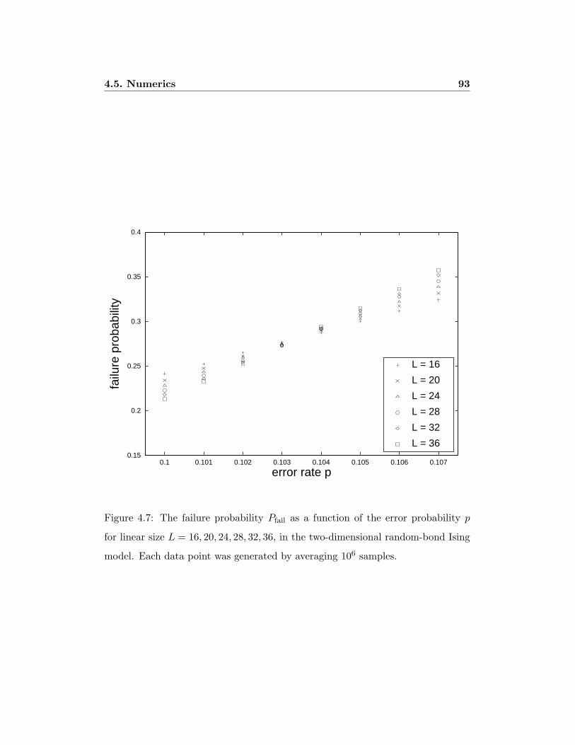
4.5. Numerics 93
0.15
0.2
0.25
0.3
0.35
0.4
0.1 0.101 0.102 0.103 0.104 0.105 0.106 0.107
failu
re p
roba
bilit
y
error rate p
L = 16
L = 20
L = 24
L = 28
L = 32
L = 36
Figure 4.7: The failure probability Pfail as a function of the error probability p
for linear size L = 16, 20, 24, 28, 32, 36, in the two-dimensional random-bond Ising
model. Each data point was generated by averaging 106 samples.

4.5. Numerics 94
0.15
0.2
0.25
0.3
0.35
0.4
0.1 0.101 0.102 0.103 0.104 0.105 0.106 0.107
failu
re p
roba
bilit
y
error rate p
L = 15
L = 19
L = 23
L = 27
L = 31
L = 35
Figure 4.8: The failure probability Pfail as a function of the error probability p
for linear size L = 15, 19, 23, 27, 31, 35, in the two-dimensional random-bond Ising
model. Each data point was generated by averaging 106 samples.

4.5. Numerics 95
where x = (p − pc0)L1/ν0 , adopting a quadratic approximation to the scaling
function f(x) in the vicinity of x = 0. (In the range of x we considered, the
quadratic term is small but not quite negligible.) For even L ranging from 22 to
42, our fit found
pc0 = .10330± .00002 ,
ν0 = 1.49± .02 , (4.40)
where the quoted errors are one-sigma statistical errors. For odd L ranging from
21 to 37, our fit found
pc0 = .10261± .00003 ,
ν0 = 1.46± .02 . (4.41)
The discrepancy between the values of pc0 for even and odd L indicates a non-
negligible finite-size effect.
On closer examination, we see evidence for small but detectable violations of
our scaling ansatz in both the even and odd data sets. These violations are very
well accounted for by the modified ansatz
Pfail = A+Bx+ Cx2
+
Deven · L−1/µeven (L even) ,
Dodd · L−1/µodd (L odd) ,(4.42)
which includes a nonuniversal additive correction to Pfail at criticality, different for
even and odd sizes. Fitting the modified ansatz to the data for even L ranging

4.5. Numerics 96
0.2
0.22
0.24
0.26
0.28
0.3
0.32
0.34
0.36
0.38
-0.04 -0.03 -0.02 -0.01 0 0.01 0.02 0.03 0.04 0.05
mod
ified
failu
re p
roba
bilit
y
rescaled error rate
Figure 4.9: The failure probability Pfail, with the nonuniversal correction of
eq. (4.42) subtracted away, as a function of the scaling variable x = (p− pc0)L1/ν0
for the two-dimensional random-bond Ising model, where pc0 and ν0 are deter-
mined by the best fit to the data. A two-sigma error bar is shown for each point.
The data for values of L from 2 to 42 lie on a single line, indicating that the (small)
scaling violations are well accounted for by our ansatz.

4.5. Numerics 97
from 2 to 42, we find
pc0 = .10309± .00003 ,
ν0 = 1.461± .008 ,
Deven = 0.165± .002 , µeven = 0.71± .01 . (4.43)
Fitting to the data for odd L ranging from 3 to 37, we find
pc0 = .10306± .00008 ,
ν0 = 1.463± .006 ,
Dodd = −.053± .003 , µodd = 2.1± .3 . (4.44)
In Figure 4.9 we show the data for all values of L and p; using the values of pc0, ν0,
D, and µ found in our fits, we have plotted Pfail, with the nonuniversal correction of
eq. (4.42) subtracted away, as a function of the scaling variable x = (p−pc0)L1/ν0 .
All of the data lie on a single line, indicating that residual scaling violations are
quite small. Furthermore, the agreement between the values of pc0 and ν0 extracted
from the even and odd data sets, which were fit independently, indicates that our
extrapolation to large L is reasonable, and that the statistical errors in eq. (4.43,
4.44) do not seriously underestimate the actual errors in our measurement. A
plausible conclusion is that
pc0 = .1031± .0001 ,
ν0 = 1.46± .01 . (4.45)
An earlier measurement reported by Kawashima and Rieger found [44]
pc0 = .104± .001 ,
ν0 = 1.30± .02 ; (4.46)
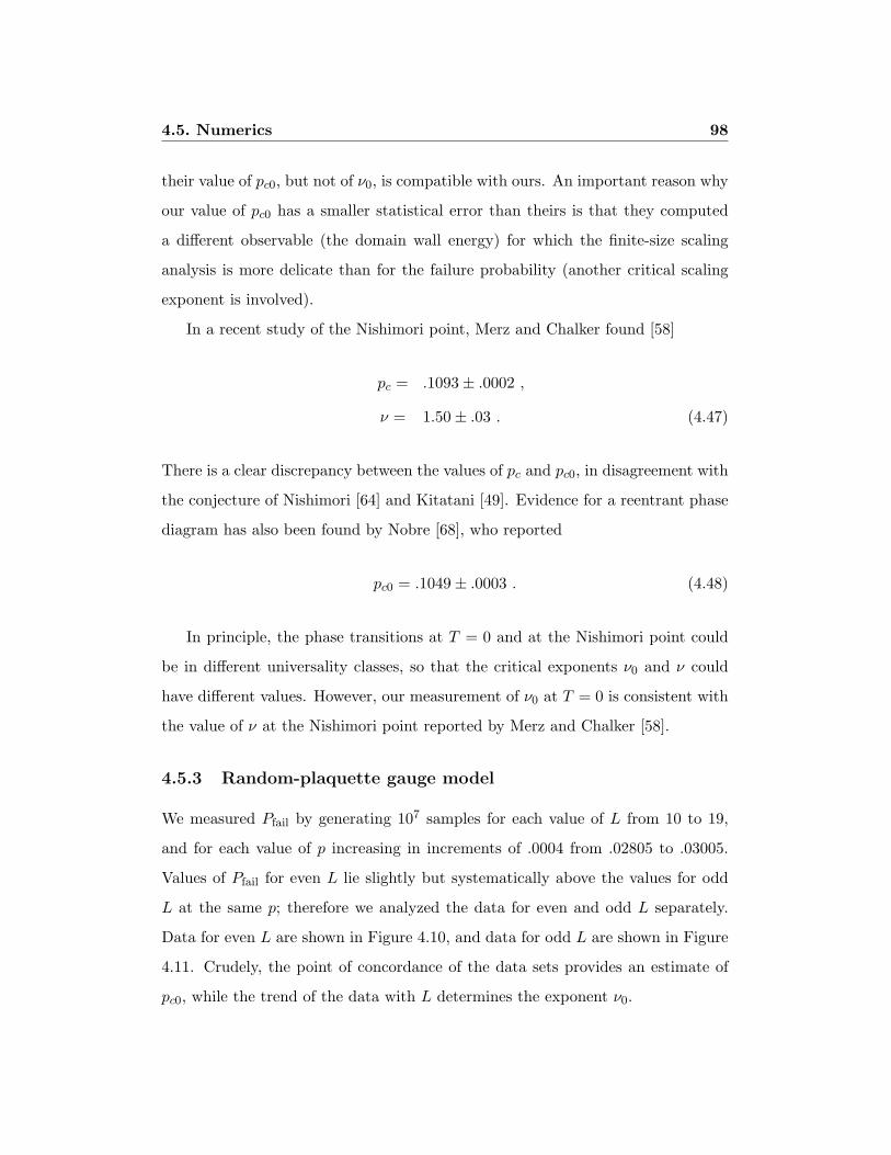
4.5. Numerics 98
their value of pc0, but not of ν0, is compatible with ours. An important reason why
our value of pc0 has a smaller statistical error than theirs is that they computed
a different observable (the domain wall energy) for which the finite-size scaling
analysis is more delicate than for the failure probability (another critical scaling
exponent is involved).
In a recent study of the Nishimori point, Merz and Chalker found [58]
pc = .1093± .0002 ,
ν = 1.50± .03 . (4.47)
There is a clear discrepancy between the values of pc and pc0, in disagreement with
the conjecture of Nishimori [64] and Kitatani [49]. Evidence for a reentrant phase
diagram has also been found by Nobre [68], who reported
pc0 = .1049± .0003 . (4.48)
In principle, the phase transitions at T = 0 and at the Nishimori point could
be in different universality classes, so that the critical exponents ν0 and ν could
have different values. However, our measurement of ν0 at T = 0 is consistent with
the value of ν at the Nishimori point reported by Merz and Chalker [58].
4.5.3 Random-plaquette gauge model
We measured Pfail by generating 107 samples for each value of L from 10 to 19,
and for each value of p increasing in increments of .0004 from .02805 to .03005.
Values of Pfail for even L lie slightly but systematically above the values for odd
L at the same p; therefore we analyzed the data for even and odd L separately.
Data for even L are shown in Figure 4.10, and data for odd L are shown in Figure
4.11. Crudely, the point of concordance of the data sets provides an estimate of
pc0, while the trend of the data with L determines the exponent ν0.
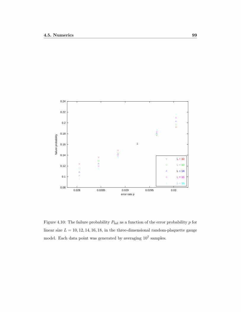
4.5. Numerics 99
0.08
0.1
0.12
0.14
0.16
0.18
0.2
0.22
0.24
0.028 0.0285 0.029 0.0295 0.03
failu
re p
roba
bilit
y
error rate p
L = 10
L = 12
L = 14
L = 16
L = 18
Figure 4.10: The failure probability Pfail as a function of the error probability p for
linear size L = 10, 12, 14, 16, 18, in the three-dimensional random-plaquette gauge
model. Each data point was generated by averaging 107 samples.

4.5. Numerics 100
0.06
0.08
0.1
0.12
0.14
0.16
0.18
0.2
0.028 0.0285 0.029 0.0295 0.03
failu
re p
roba
bilit
y
error rate p
L = 11
L = 13
L = 15
L = 17
L = 19
Figure 4.11: The failure probability Pfail as a function of the error probability p for
linear size L = 11, 13, 15, 17, 19, in the three-dimensional random-plaquette gauge
model. Each data point was generated by averaging 107 samples.

4.5. Numerics 101
0.06
0.08
0.1
0.12
0.14
0.16
0.18
0.2
-0.02 -0.015 -0.01 -0.005 0 0.005 0.01 0.015 0.02
failu
re p
roba
bilit
y
rescaled error rate
Figure 4.12: The failure probability Pfail as a function of the scaling variable
x = (p − pc0)L1/ν0 for the random-plaquette gauge model, where pc0 and ν0 are
determined by the best fit to the data. A ten-sigma error bar is shown for each
point (to demonstrate how well the points fit the given quadratic curve). Those
points with smaller error bars were averaged from 108 samples (as opposed to 107
samples for the other points). The data for all odd values of L from 11 to 19 lie
on a single curve, indicating that scaling violations are small at these lattice sizes.

4.5. Numerics 102
We did a global fit of the data to the form
Pfail = A+Bx+ Cx2 , (4.49)
where x = (p − pc0)L1/ν0 , adopting a quadratic approximation to the scaling
function f(x) in the vicinity of x = 0. For L ranging from 10 to 19, our fit found
pc0 = .029351± .000014 , ν0 = 0.980± .018 (L even) ,
pc0 = .028992± .000002 , ν0 = 1.006± .003 (L odd) , (4.50)
where the quoted errors are one-sigma statistical errors. The results for even and
odd L are incompatible, indicating a non-negligible finite-size effect.
We believe that our analysis for odd L is likely to be more reliable; finite size
effects are enhanced for even L, the case in which the failure probability is larger.
All of the odd-L data are shown in Figure 4.12, with Pfail plotted as a function
of x = (p − pc0)L1/ν0 , where pc0 and ν0 are determined by our fit. The data fit
a single curve, indicating that scaling violations are small. (Scaling violations are
more discernable in the even-L data set.) A reasonable conclusion is that
pc0 = .0290± .0001 ,
ν0 = 1.00± .02 . (4.51)
4.5.4 Anisotropic random-plaquette gauge model
We also measured Pfail for differing values of the bit-flip (or phase-flip) error
probability p and the measurement error probability q. This corresponds to a
three-dimensional random-plaquette gauge model with differing disorder strength
in the horizontal and vertical plaquettes.
For fixed values of p and q, Pfail was computed for lattices over a range of
horizontal sizes, each with an optimal vertical size (corresponding to the number
of measurements performed on the lattice before performing error correction by
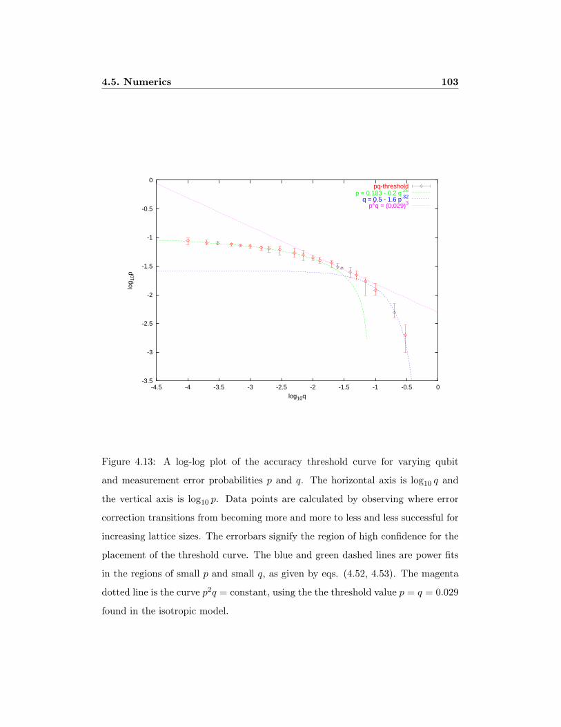
4.5. Numerics 103
-3.5
-3
-2.5
-2
-1.5
-1
-0.5
0
-4.5 -4 -3.5 -3 -2.5 -2 -1.5 -1 -0.5 0
log 1
0p
log10q
pq-thresholdp = 0.103 - 0.2 q.26
q = 0.5 - 1.6 p.32
p2q = (0.029)3
Figure 4.13: A log-log plot of the accuracy threshold curve for varying qubit
and measurement error probabilities p and q. The horizontal axis is log10 q and
the vertical axis is log10 p. Data points are calculated by observing where error
correction transitions from becoming more and more to less and less successful for
increasing lattice sizes. The errorbars signify the region of high confidence for the
placement of the threshold curve. The blue and green dashed lines are power fits
in the regions of small p and small q, as given by eqs. (4.52, 4.53). The magenta
dotted line is the curve p2q = constant, using the the threshold value p = q = 0.029
found in the isotropic model.

4.5. Numerics 104
the Edmonds perfect matching algorithm [29, 6]). By observing whether Pfail got
larger or smaller with increasing lattice sizes, we could infer whether a particular
pair of values for p and q was above or below the threshold curve. From this
data, we could then generate a (rough) plot of the accuracy threshold curve in the
pq-plane. Our conclusions are summed up in Figure 4.13. We have included the
isotropic point p = q = 0.029 determined from the previous section.
We have fit our data to various curves involving either powers or entropies of
p and q, but given the levels of uncertainty in the data, we cannot conclude that
any of these generated fits really describes the threshold curve. However, we can
separately state the small p and small q behavior of this curve:
q ≈ 0.5− 1.6p0.32 (for small p) (4.52)
p ≈ 0.103− 0.2q0.26 (for small q) (4.53)
Also, we observe that for moderate values of p and q (close to the isotropic point
p = q = 0.029), the threshold data is well fit by p2q = constant.
4.5.5 The failure probability at finite temperature
Our numerical studies of the RBIM and the RPGM were restricted to the T = 0
axis. We calculated the failure probability to estimate the critical disorder strength
pc0 and the critical exponent ν0. Here we will describe how the calculation of the
failure probability could be extended to nonzero temperature.
To calculate the failure probability in the zero-temperature RBIM, we generate
a sample by specifying a one-chain E of antiferromagnetic links, and then we
construct the one-chain E′ of minimal energy with the same boundary as E. Failure
occurs if the cycle D = E + E′ is homologically nontrivial.
At nonzero temperature we should construct E′ to belong to the homology
class that minimizes free energy rather than energy. For a given sample with
antiferromagnetic one-chain E, the free energy F (E, h) of homology class h is

4.5. Numerics 105
found by summing over domain wall one-chains E′ such that E + E′ ∈ h:
exp[−βF (E, h)] = Z(E, h) =∑
E′:E+E′∈h
e−βHE , (4.54)
where HE denotes the Hamiltonian eq. (4.1) with antiferromagnetic chain E. If the
trivial homology class h = e has the lowest free energy, then the sample is a “suc-
cess”; otherwise it is a “failure.” We can estimate the failure probability Pfail(p, T )
by randomly generating many samples, and determining for each whether it is a
success or a failure.
For the random bond Ising model on a torus, the sum eq. (4.3) includes only
the chains E′ such that E + E′ is in the trivial homology class. To sum over the
class h, we can augment E by adding to it a representative of h. For each h, we
can computeZ(E, h)Z(E, e)
= exp[− β
(F (E, h)− F (E, e)
)]; (4.55)
the sample E is a success if this ratio of partition functions is less than one for
each h 6= e.
The ratio is the thermal expectation value 〈Oh〉K of an observable Oh that
“inserts a domain wall” wrapping around a cycle C representing h. That is, the
effect of Oh is to flip the sign of the bond variable τij for each bond 〈ij〉 in C:
Oh = exp
−2K∑〈ij〉∈C
τijSiSj
. (4.56)
In principle, we could measure 〈Oh〉K by the Monte Carlo method, generating
typical configurations in the thermal ensemble of HE , and evaluating Oh in these
configurations. Unfortunately, this method might not produce an accurate mea-
surement, because the configurations that dominate 〈Oh〉K may be exponentially
rare in the thermal ensemble — a configuration with excited bonds on C can
have an exponentially large value of Oh that overcomes exponential Boltzmann
suppression.

4.6. Conclusions 106
One solution to this problem is to express Z(E, h)/Z(E, e) as a product of
quantities, each of which can be evaluated accurately by Monte Carlo. Let e =
P0, P1, P2, . . . Pk−1, Pk = C be a sequence of open chains interpolating between
the empty chain and the cycle C, where Pj+1−Pj contains just a single bond. We
may writeZ(E, h)Z(E, e)
=Z(E,P1)Z(E,P0)
· Z(E,P2)Z(E,P1)
· · · · · Z(E,Pk)Z(E,Pk−1)
. (4.57)
Each ratio Z(E,Pj+1)/Z(E,Pj) is the expectation value of an operator that acts
on a single bond, evaluated in the thermal ensemble of the Hamiltonian with anti-
ferromagnetic bonds on the chain E +Pj ; this expectation value can be evaluated
by Monte Carlo with reasonable computational resources. (For an application of
this trick in a related setting, see [25].)
Using this method, we can determine whether Z(E, h)/Z(E, e) exceeds one for
any h 6= e and hence whether the sample E is a success or a failure. Generating
many samples, we can estimate Pfail(p, T ). In principle, then we can calculate
the failure probability for the optimal recovery scheme, in which p and T obey
Nishimori’s relation. By a similar method, we can calculate the failure probability
for the RPGM. However, we have not attempted this calculation.
4.6 Conclusions
The three-dimensional random-plaquette gauge model, and the analogous antisym-
metric tensor models in higher dimensions, provide new examples of multicritical
points with strong disorder. These models have phase diagrams that qualitatively
resemble the phase diagram of the two-dimensional random-bond Ising model.
Our results indicate that the boundary between the ferromagnetic and param-
agnetic phases of the RBIM is reentrant rather than vertical below the Nishimori
line. If the disorder strength p satisfies pc0 < p < pc, then the ground state of the
spin system does not have long-range order. As the temperature T increases with

4.6. Conclusions 107
p fixed, long-range order is first restored, and then lost again as the temperature
increases further. At T = 0 the spins are frozen in a disordered state driven by
quenched randomness. But apparently this ground state is entropically unfavor-
able — at low but nonzero temperature typical states in the thermal ensemble
have long-range ferromagnetic order.
This behavior seems less remarkable when considered from the viewpoint of our
error recovery protocol. For given p and a specified error syndrome, the recovery
method with optimal success probability proceeds by inferring the most likely
homology class of errors consistent with the syndrome. There is no a priori reason
for the most likely single error pattern (the ground state) to belong to the most
likely error homology class (the class with minimal free energy) even in the limit
of a large sample. Our numerical results indicate that for error probability p such
that pc0 < p < pc, the probability that the ground state does not lie in the most
likely homology class remains bounded away from zero as L→∞.
In our numerical studies of the RBIM and RPGM at zero temperature, we
have computed a homological observable, the failure probability. This observable
has advantages over, say, the domain wall energy, because it obeys a particularly
simple finite-size-scaling ansatz. Therefore, we have been able to determine the
critical disorder strength pc0 and the critical exponent ν0 to good accuracy with
relatively modest computational resources.
Not surprisingly, our numerical values for pc0 are notably larger than rigorous
lower bounds derived using crude combinatoric arguments in [26]: pc0 ≈ .1031
compared with the bound pc0 ≥ .0373 in the RBIM, and pc0 ≈ .0290 compared
with pc0 ≥ .0114 in the RPGM.
The zero-temperature critical disorder strength pc0 is a lower bound on the
value of the critical disorder strength pc along the Nishimori line, and of special
interest because of its connection with the accuracy threshold for robust storage
of quantum information. Our result means that stored quantum data can be
preserved with arbitrarily good fidelity if, in each round of syndrome measurement,
qubit errors and syndrome measurement errors are independently and identically

4.6. Conclusions 108
distributed, with error probability per qubit and per syndrome bit both below
2.9%. For qubit errors and measurement errors occurring at differing rates, an
accuracy threshold has been inferred by analyzing an anisotropic random-plaquette
gauge model, with differing disorder strength for horizontal and vertical plaquettes.
Future work is needed to more conclusively identify the tradeoff curve in this
model. Relating these threshold error rates to fidelity requirements for quantum
gates requires further analysis of the sort discussed in [26].
We have also measured the critical exponent ν0 that controls the divergence
of the correlation length as p approaches pc0, finding ν0 ≈ 1.46 in the RBIM and
ν0 ≈ 1.0 in the RPGM. The value of ν0 is also relevant to the efficacy of quantum
error correction — through its connection with finite-size scaling, ν0 determines
how large the code block should be to achieve a specified storage fidelity, for p less
than but close to pc0.
Quantum computers are believed to be more powerful than classical comput-
ers — classical computers are unable to simulate quantum computers efficiently.
The accuracy threshold for quantum memory is a fascinating phase transition,
separating a low-noise quantum phase from a high-noise classical phase. In this
paper, we have described one way to analyze this phase transition using methods
from traditional statistical physics. Furthermore, the connection with quantum
memory provides an enlightening new perspective on local spin and gauge systems
with strong quenched disorder.

109
Chapter 5
Protecting topological quantum information
by local rules
5.1 Abstract
Kitaev’s surface codes (e.g., toric codes and planar codes) [48] are two-dimensional
topological quantum error-correcting codes which have the attractive features of
requiring only local measurements and being robust to local clusters of errors.
Previously [26], processing the error syndromes required global communication
and reasonably fast classical computation, with a resource cost (in processing time)
that scaled polynomially with the size of the lattice. In this work, we present a
fairly simple set of local rules that handle the error syndrome processing (so that
much of the computation and communication can be done in parallel). We make
use of several ideas from a proof by Gacs [31, 33, 39] of the existence of robust
one-dimensional classical cellular automata to demonstrate analytically that an
accuracy threshold exists for storing quantum memory in our system. We show
numerical results that suggest that the threshold for bit flip or phase flip errors
per time step is at least 10−4.

5.2. Introduction 110
5.2 Introduction
Our aim is to present a fault-tolerant scheme for preserving quantum memory
with only local controls on a two-dimensional lattice of spins. We begin with a
discussion of robust classical cellular automata in Section 5.3 and highlight work
by Gacs. In Section 5.4 we outline our model and illustrate how the quantum
error syndromes in toric codes are similar to those in a classical one-dimensional
array. The syndrome error processing is detailed in Section 5.5, and the main
rules for local error correction are laid out in Section 5.6. Our analytical proof
of an accuracy threshold is developed in sections 5.7 and 5.8, and we present
results from numerical simulations in Section 5.9. We conclude in Section 5.10
with a comparison of required resources for local error correction in classical and
quantum memory, as well as suggestions for future work.
5.3 Robust cellular automata
There are numerous examples of cellular automata (networks of cells with local
update rules) which exhibit complex behavior, rich structures, and even universal
computation. For example, Conway’s game of Life [14] defines a very simple set
of rules on a rectangular grid of cells, each storing only one bit, where each cell
updates based on its present state and the sum of its eight nearest neighbors. It
is possible to create configurations which will, for example, continuously grow at
an ever increasing rate or implement an arbitrary computation. (See [71] for a
fascinating overview of this topic.) In a one-dimensional array of binary cells with
nearest-neighbor interactions, Cook has demonstrated that a particular simple set
of rules can carry out universal computation [57]. While not strictly a cellular
automaton, determining consistency of a partial revealing of a Minesweeper game
has been shown by Kaye [46] to be equivalent to the NP-complete SAT problem.
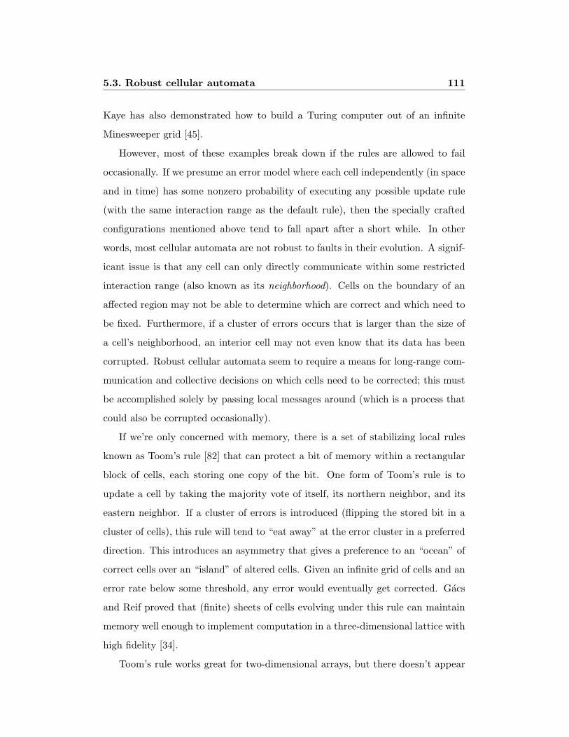
5.3. Robust cellular automata 111
Kaye has also demonstrated how to build a Turing computer out of an infinite
Minesweeper grid [45].
However, most of these examples break down if the rules are allowed to fail
occasionally. If we presume an error model where each cell independently (in space
and in time) has some nonzero probability of executing any possible update rule
(with the same interaction range as the default rule), then the specially crafted
configurations mentioned above tend to fall apart after a short while. In other
words, most cellular automata are not robust to faults in their evolution. A signif-
icant issue is that any cell can only directly communicate within some restricted
interaction range (also known as its neighborhood). Cells on the boundary of an
affected region may not be able to determine which are correct and which need to
be fixed. Furthermore, if a cluster of errors occurs that is larger than the size of
a cell’s neighborhood, an interior cell may not even know that its data has been
corrupted. Robust cellular automata seem to require a means for long-range com-
munication and collective decisions on which cells need to be corrected; this must
be accomplished solely by passing local messages around (which is a process that
could also be corrupted occasionally).
If we’re only concerned with memory, there is a set of stabilizing local rules
known as Toom’s rule [82] that can protect a bit of memory within a rectangular
block of cells, each storing one copy of the bit. One form of Toom’s rule is to
update a cell by taking the majority vote of itself, its northern neighbor, and its
eastern neighbor. If a cluster of errors is introduced (flipping the stored bit in a
cluster of cells), this rule will tend to “eat away” at the error cluster in a preferred
direction. This introduces an asymmetry that gives a preference to an “ocean” of
correct cells over an “island” of altered cells. Given an infinite grid of cells and an
error rate below some threshold, any error would eventually get corrected. Gacs
and Reif proved that (finite) sheets of cells evolving under this rule can maintain
memory well enough to implement computation in a three-dimensional lattice with
high fidelity [34].
Toom’s rule works great for two-dimensional arrays, but there doesn’t appear

5.4. Toric codes and implementation 112
to be any direct analogue in one-dimensional arrays. It had been conjectured
that robust one-dimensional cellular automata for storing memory did not exist
[52] (known as the “Positive Rates Conjecture”). Eventually, large clusters of
errors would occur that would be uncorrectable, because the boundaries in one-
dimensional arrays are zero-dimensional points, and it seems impossible to make
a reliable local decision around the boundary of which side is valid and which side
needs to be corrected. Gacs proved this conjecture wrong in some amazing work
[31, 33] that is unfortunately hard to read through. We highly recommend Gray’s
reader’s guide [39] as a source for learning about the main ideas of Gacs’s proof,
along with a simplified model of his construction.
5.4 Toric codes and implementation
Here we briefly review the structure of toric codes in the stabilizer formalism and
suggest how to construct a quantum system with this encoding.
5.4.1 Toric code stabilizers
Toric codes are discussed in Section 4.4.1. The important features are repeated
here. Qubits are placed on the edges of an L×L rectangular lattice. The stabilizers
are generated by X ⊗ X ⊗ X ⊗ X around each plaquette and Z ⊗ Z ⊗ Z ⊗ Z
around each site. (See Figure 4.3 for a diagram of these operators.) An odd
number of phase flips acting on the qubits around a given lattice site causes the
XXXX syndrome measurement to change sign. Likewise, an odd number of bit
flips acting on the qubits around a plaquette (or equivalently, around a site on
the dual lattice) causes the corresponding ZZZZ measurement to change sign.
A long chain of errors is detected only at its endpoints, because there are an
even number of errors around interior sites, which commute with those syndrome
measurements. The bit flip and phase flip errors appear as one-dimensional chains
with zero-dimensional (point) boundaries, which can be related to classical errors

5.4. Toric codes and implementation 113
in a one-dimensional array. The primary difference is that these errors live on a
two-dimensional surface, and any trivial loop of errors (a closed chain that can be
contracted down to a point) is in the stabilizer group and thus acts as the identity
on the encoded subspace.
5.4.2 Hardware layout
We consider implementing a toric code by arranging a rectangular lattice of spins
on a torus. For sufficiently large lattices, the behavior of toric codes is well approx-
imated by that of planar codes (in particular, in terms of the value of the accuracy
threshold), so it is possible to use a planar lattice in practice, but we will assume
a toric layout in this work. The spin-12 particles are placed on each edge, or link,
of the lattice. Thus, an L×L lattice consists of 2L2 spins. At each vertex, or site,
we place a classical processor that will be responsible for measuring the four spins
on its neighboring links and executing phase flips on those links when needed.
We also place a classical processor at every site of the dual lattice (which is
obtained by rotating all of the links by 90 degrees). This set of processors is
responsible for measuring the four neighboring spins around each site (on the dual
lattice), as well as executing bit flips when needed. Since the phase flip and bit flip
error correction can be performed independently of one another, we will focus on
just phase flip errors in this model, recognizing that an identical process is going
on simultaneously to handle bit flip errors.
5.4.3 Error model
In between each error correction step, we assume that every spin independently
has a probability pphase of undergoing a phase flip (and likewise, independently a
probability pbit of undergoing a bit flip). Since we will focus on phase flips (with
bit flips being handled separately and simultaneously), we will simply describe
the phase flip error rate as p. Also, we assume that each syndrome measurement
of XXXX independently has a probability q of being incorrect. We wish to

5.5. Processor memory 114
demonstrate that there exist thresholds for p and q which allow arbitrarily high
fidelity for local error correction. We will assume that the classical processors and
memory are very reliable. (In Section 5.8.3, we briefly discuss how this assumption
could be relaxed.)
5.5 Processor memory
Following Gacs’s constructions [31, 33, 32], we impart a hierarchy on the layout of
processors. We treat each processor as a cell, which will update its state based on
its memory contents along with the memory contents of its eight nearest neighbors
(north, northeast, east, southeast, south, southwest, west, and northwest). Rect-
angular groups of Q×Q cells are identified as belonging to a colony. Rectangular
groups of Q×Q colonies are identified as belonging to a super-colony. This hier-
archy continues on to higher and higher levels (until the whole lattice is included).
We will assume that the linear lattice size L = Qk for some integer k. Errors will
later be classified within a hierarchy of levels as well, and we will demonstrate how
each level of errors will be handled by the corresponding level of colonies.
Several constants are hardcoded into the device, which will be explained below.
They include Q (the colony size), U (the work period), fC (the threshold for a cell’s
count), and fN (the threshold for a neighboring cell’s count). As a reference, we
will later choose Q = 16, U = 400, fC = 4/5, and fN = 1/5 for deriving an
accuracy threshold.
5.5.1 Memory fields
Every cell has the following fields of memory: Address, Age, and Syndromes.
Address has two subfields x and y that identify the horizontal and vertical ad-
dress of the cell in its colony. Age is a local “clock” that counts the number of time
steps in a work period (of length U). Syndromes has nine subfields (each just a
bit), which store the most recent syndrome measurements at this site and its eight

5.5. Processor memory 115
Table 5.1: Processor memory fields for local error correction of toric codes
field name size description
Address 2 dlogQe horizontal and vertical address in colony
Age dlogUe local clock running from 0 to (U - 1)
Syndromes 9 syndrome at this site and its neighbors
Count 9 dlogUe coarse-grained count of syndrome history
CountSignal 8 value of neighboring colony’s syndrome
NewCountSignal 8 temporary storage of value for CountSignal
FlipSignal 8 signal for flipping at end of a work period
NewFlipSignal 8 temporary storage of value for FlipSignal
neighboring sites. A cell’s most recent measurement is denoted Syndromes.C, and
the other subfields are Syndromes.N, Syndromes.E, Syndromes.S, Syndromes.W,
Syndromes.NE, Syndromes.SE, Syndromes.SW, and Syndromes.NW, referring to the
cell’s northern, eastern, southern, western, and four diagonal neighbors, respec-
tively.
The following fields of memory are also needed at some particular cells: Count,
CountSignal, NewCountSignal, FlipSignal, and NewFlipSignal. The Count
field has nine subfields (similar to Syndromes) which keep track of how often a
syndrome is present at the center of a colony (either the current colony or one
of its eight neighboring colonies) during a work period. The four “signal” fields
provide a means of communication between colonies (traveling one cell per time
step). They each have eight subfields corresponding to the eight directions making
up the neighborhood of a cell. The CountSignal field contains the information
of whether syndromes are present or absent at a particular time step in the cen-
ters of neighboring colonies. The FlipSignal field contains a signal for control-
ling flips across colonies at the end of a work period. The NewCountSignal and
NewFlipSignal fields provide temporary storage of neighbors’ values, before up-
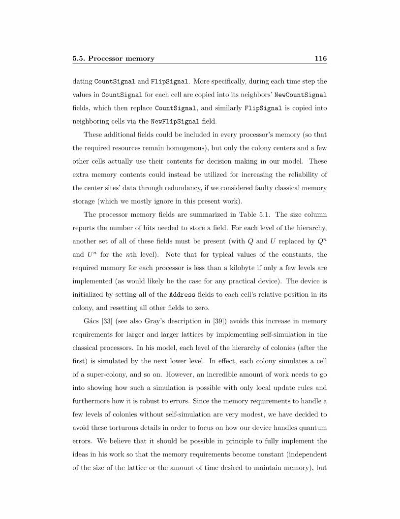
5.5. Processor memory 116
dating CountSignal and FlipSignal. More specifically, during each time step the
values in CountSignal for each cell are copied into its neighbors’ NewCountSignal
fields, which then replace CountSignal, and similarly FlipSignal is copied into
neighboring cells via the NewFlipSignal field.
These additional fields could be included in every processor’s memory (so that
the required resources remain homogenous), but only the colony centers and a few
other cells actually use their contents for decision making in our model. These
extra memory contents could instead be utilized for increasing the reliability of
the center sites’ data through redundancy, if we considered faulty classical memory
storage (which we mostly ignore in this present work).
The processor memory fields are summarized in Table 5.1. The size column
reports the number of bits needed to store a field. For each level of the hierarchy,
another set of all of these fields must be present (with Q and U replaced by Qn
and Un for the nth level). Note that for typical values of the constants, the
required memory for each processor is less than a kilobyte if only a few levels are
implemented (as would likely be the case for any practical device). The device is
initialized by setting all of the Address fields to each cell’s relative position in its
colony, and resetting all other fields to zero.
Gacs [33] (see also Gray’s description in [39]) avoids this increase in memory
requirements for larger and larger lattices by implementing self-simulation in the
classical processors. In his model, each level of the hierarchy of colonies (after the
first) is simulated by the next lower level. In effect, each colony simulates a cell
of a super-colony, and so on. However, an incredible amount of work needs to go
into showing how such a simulation is possible with only local update rules and
furthermore how it is robust to errors. Since the memory requirements to handle a
few levels of colonies without self-simulation are very modest, we have decided to
avoid these torturous details in order to focus on how our device handles quantum
errors. We believe that it should be possible in principle to fully implement the
ideas in his work so that the memory requirements become constant (independent
of the size of the lattice or the amount of time desired to maintain memory), but
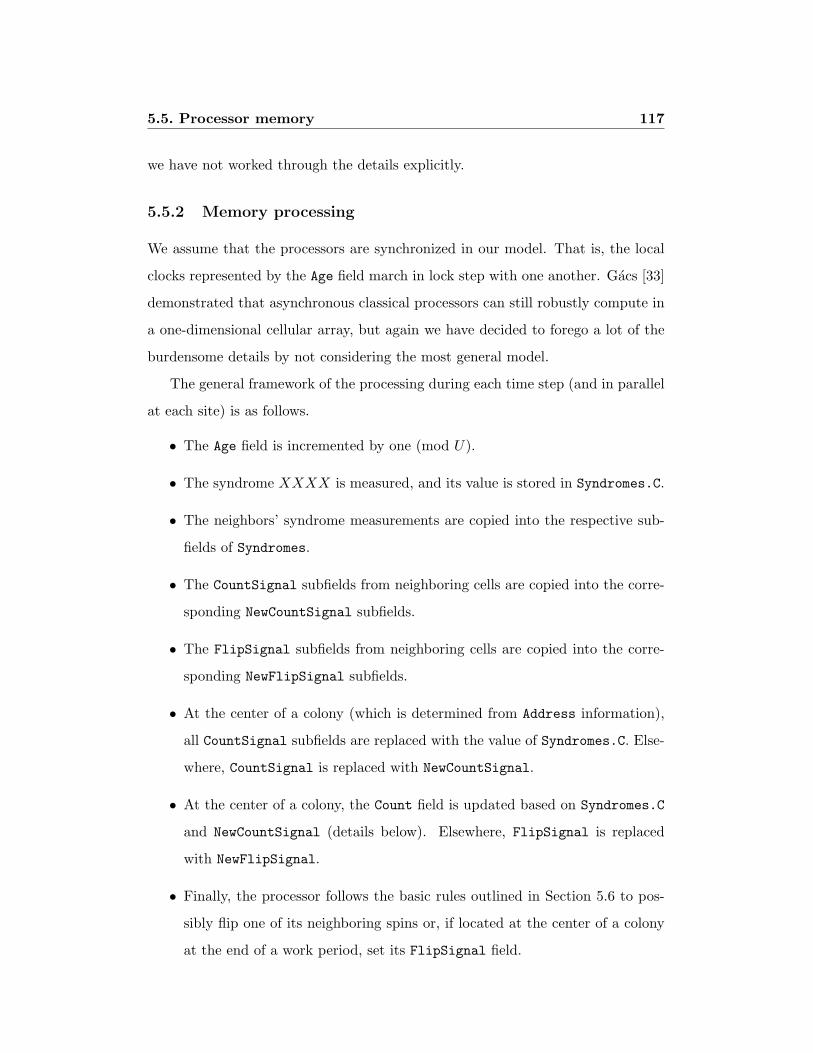
5.5. Processor memory 117
we have not worked through the details explicitly.
5.5.2 Memory processing
We assume that the processors are synchronized in our model. That is, the local
clocks represented by the Age field march in lock step with one another. Gacs [33]
demonstrated that asynchronous classical processors can still robustly compute in
a one-dimensional cellular array, but again we have decided to forego a lot of the
burdensome details by not considering the most general model.
The general framework of the processing during each time step (and in parallel
at each site) is as follows.
• The Age field is incremented by one (mod U).
• The syndrome XXXX is measured, and its value is stored in Syndromes.C.
• The neighbors’ syndrome measurements are copied into the respective sub-
fields of Syndromes.
• The CountSignal subfields from neighboring cells are copied into the corre-
sponding NewCountSignal subfields.
• The FlipSignal subfields from neighboring cells are copied into the corre-
sponding NewFlipSignal subfields.
• At the center of a colony (which is determined from Address information),
all CountSignal subfields are replaced with the value of Syndromes.C. Else-
where, CountSignal is replaced with NewCountSignal.
• At the center of a colony, the Count field is updated based on Syndromes.C
and NewCountSignal (details below). Elsewhere, FlipSignal is replaced
with NewFlipSignal.
• Finally, the processor follows the basic rules outlined in Section 5.6 to pos-
sibly flip one of its neighboring spins or, if located at the center of a colony
at the end of a work period, set its FlipSignal field.

5.6. Local rules 118
Rather than just keeping a simple running total of error syndromes being
present or absent (denoted as on or off), we have the Count field keep a coarse-
grained count in the following manner. We choose U = b2 (where b will be de-
termined by the definition of low-level errors in our proof) and divide the work
period U into b intervals of length b. The Count subfields are each divided into
two sections of size dlog be. The first section stores a running count of syndrome
measurements during each interval. At the end of each interval (when Age ≡ 0
(mod b)), the second section is incremented if the first section totals at least fCb
(for Count.C) or at least fNb (for the other eight Count subfields). The first sec-
tion is then reset to 0. Finally, at the end of the work period, a Count subfield is
considered to be on if its second section is at least fCb or fNb, as before. Thus, a
syndrome is considered to be present in the colony during a work period if, during
at least fC of the intervals, it is present at the center for at least fC of the time
steps.
The FlipSignal field stores the decision of a colony center at the end of a work
period of whether to introduce a flip along a path to a neighboring colony. This
signal is propagated cell by cell until it reaches another colony center after Q time
steps. All sites with a FlipSignal on then perform the desired flip in unison, and
FlipSignal is reset to zero (or off). In this manner, a colony center can affect
a chain of flips between two neighboring colonies. An analogous process occurs
every U2 time steps between neighboring super-colonies, and similarly for higher
levels in the hierarchy.
5.6 Local rules
The basic rules are as follows. The first two sets of rules handle flips of qubits
along the border of neighboring colonies. The remaining rules handle the interior
qubits in a colony. Each qubit is only ever controlled by a single processor. When
there is an option in terms of which qubit to flip (e.g., north or east), the direction

5.6. Local rules 119
could be chosen either at random or always to be a fixed value. In our simulations,
we chose the direction that pointed away from the closest border to the colony
(which was determined by Address information).
(W border) If Address.x == 0, then:
if Syndromes.C is off, do nothing
else if Syndromes.NW is on, flip west
else if Syndromes.W is on, flip west
else if Syndromes.SW is on, flip west
else, continue below
(S border) If Address.y == 0, then:
if Syndromes.C is off, do nothing
else if Syndromes.SW is on, flip south
else if Syndromes.S is on, flip south
else if Syndromes.SE is on, flip south
else, continue below

5.6. Local rules 120
(SW quadrant) If Address.x < bQ2 c and Address.y < bQ2 c, then:
if Syndromes.C is off, do nothing
else if Syndromes.S is on, do nothing
else if Syndromes.W is on, do nothing
else if Syndromes.N is on, flip north
else if Syndromes.E is on, flip east
else if Syndromes.SW is on, do nothing
else if Syndromes.NW is on, flip north
else if Syndromes.SE is on, flip east
else, flip north or east
(W corridor) If Address.x < bQ2 c and Address.y == bQ2 c, then:
if Syndromes.C is off, do nothing
else if Syndromes.S is on, do nothing
else if Syndromes.W is on, do nothing
else if Syndromes.N is on, do nothing
else if Syndromes.E is on, flip east
else if Syndromes.SW is on, do nothing
else if Syndromes.NW is on, do nothing
else, flip east

5.6. Local rules 121
(NW quadrant) If Address.x < bQ2 c and Address.y > bQ2 c, then:
if Syndromes.C is off, do nothing
else if Syndromes.W is on, do nothing
else if Syndromes.N is on, do nothing
else if Syndromes.E is on, flip east
else if Syndromes.S is on, flip south
else if Syndromes.NW is on, do nothing
else if Syndromes.NE is on, flip east
else if Syndromes.SW is on, flip south
else, flip east or south
(N corridor) If Address.x == bQ2 c and Address.y > bQ2 c, then:
if Syndromes.C is off, do nothing
else if Syndromes.W is on, do nothing
else if Syndromes.N is on, do nothing
else if Syndromes.E is on, do nothing
else if Syndromes.S is on, flip south
else if Syndromes.NW is on, do nothing
else if Syndromes.NE is on, do nothing
else, flip south
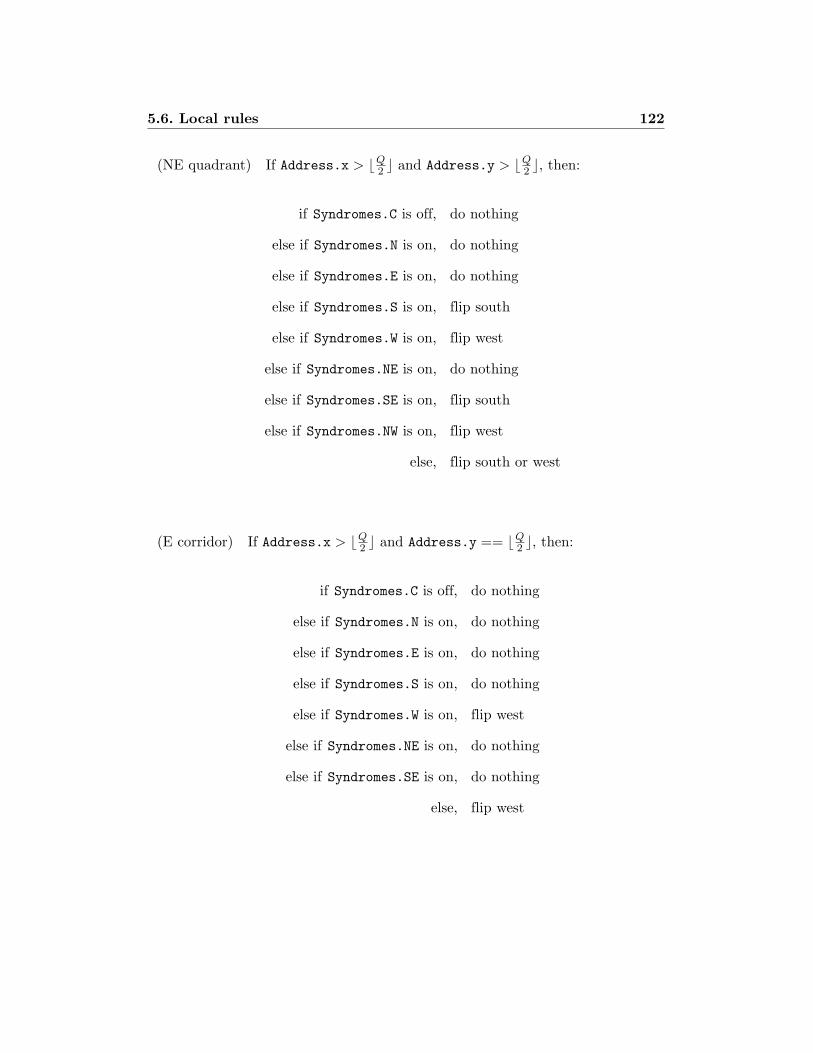
5.6. Local rules 122
(NE quadrant) If Address.x > bQ2 c and Address.y > bQ2 c, then:
if Syndromes.C is off, do nothing
else if Syndromes.N is on, do nothing
else if Syndromes.E is on, do nothing
else if Syndromes.S is on, flip south
else if Syndromes.W is on, flip west
else if Syndromes.NE is on, do nothing
else if Syndromes.SE is on, flip south
else if Syndromes.NW is on, flip west
else, flip south or west
(E corridor) If Address.x > bQ2 c and Address.y == bQ2 c, then:
if Syndromes.C is off, do nothing
else if Syndromes.N is on, do nothing
else if Syndromes.E is on, do nothing
else if Syndromes.S is on, do nothing
else if Syndromes.W is on, flip west
else if Syndromes.NE is on, do nothing
else if Syndromes.SE is on, do nothing
else, flip west
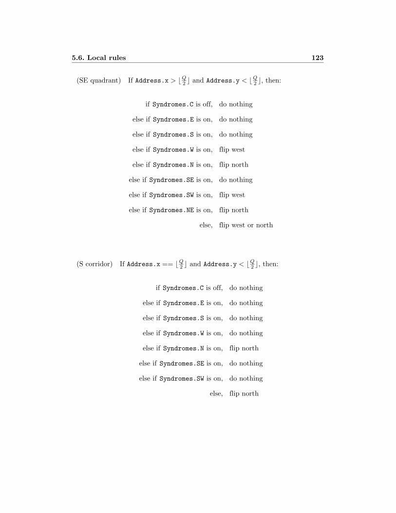
5.6. Local rules 123
(SE quadrant) If Address.x > bQ2 c and Address.y < bQ2 c, then:
if Syndromes.C is off, do nothing
else if Syndromes.E is on, do nothing
else if Syndromes.S is on, do nothing
else if Syndromes.W is on, flip west
else if Syndromes.N is on, flip north
else if Syndromes.SE is on, do nothing
else if Syndromes.SW is on, flip west
else if Syndromes.NE is on, flip north
else, flip west or north
(S corridor) If Address.x == bQ2 c and Address.y < bQ2 c, then:
if Syndromes.C is off, do nothing
else if Syndromes.E is on, do nothing
else if Syndromes.S is on, do nothing
else if Syndromes.W is on, do nothing
else if Syndromes.N is on, flip north
else if Syndromes.SE is on, do nothing
else if Syndromes.SW is on, do nothing
else, flip north

5.7. Error decomposition proof 124
(colony center) If Address.x == bQ2 c and Address.y == bQ2 c, then:
if Age == 0, execute rules for colony neighbors and update FlipSignal
else, do nothing
5.7 Error decomposition proof
In this section, we define a hierarchy of sets of errors and derive a bound in
equation (5.3) on the underlying error rates that will guarantee that higher-level
errors become increasingly rarer. In the following section, we will show how the
local update rules correct each level of errors. This section follows very closely the
proof given in Gray [39].
As introduced previously, the colony size and the work period are denoted as Q
and U . The following steps hold true provided that Q ≥ 4(a+2) and U ≥ 4(b+2),
for some positive integers a and b.
Phase flip errors occur on the edges of the lattice, where the qubits are located.
Errors in measuring the XXXX syndrome occur at the vertices of the lattice. (Bit
flip errors and ZZZZ measurement errors can be treated as occurring on the edges
and vertices of the dual lattice and can be handled analogously.) We can represent
an error as a point (x, y, t), where t corresponds to the time step we are considering,
and (x, y) corresponds to the coordinates in space of an error (either a site or the
midpoint of an edge). Both x and y are integers for measurement errors, while one
is a half-integer for phase flip errors.
Let us define two collections of points A,B as (l,m, n)-linked if there exists a
spacetime box [x, x+ l)× [y, y+m)× [t, t+ n) that contains at least one member
of A and at least one member of B. Otherwise we will say that A and B are
(l,m, n)-separated.
Let E be the set of phase flip errors and XXXX measurement errors. We will
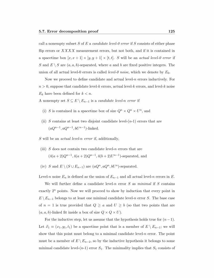
5.7. Error decomposition proof 125
call a nonempty subset S of E a candidate level-0 error if S consists of either phase
flip errors or XXXX measurement errors, but not both, and if it is contained in
a spacetime box [x, x + 1] × [y, y + 1] × [t, t]. S will be an actual level-0 error if
S and E \ S are (a, a, b)-separated, where a and b are fixed positive integers. The
union of all actual level-0 errors is called level-0 noise, which we denote by E0.
Now we proceed to define candidate and actual level-n errors inductively. For
n > 0, suppose that candidate level-k errors, actual level-k errors, and level-k noise
Ek have been defined for k < n.
A nonempty set S ⊆ E \ En−1 is a candidate level-n error if
(i) S is contained in a spacetime box of size Qn ×Qn × Un, and
(ii) S contains at least two disjoint candidate level-(n-1) errors that are
(aQn−1, aQn−1, bUn−1)-linked.
S will be an actual level-n error if, additionally,
(iii) S does not contain two candidate level-n errors that are
(4(a+ 2)Qn−1, 4(a+ 2)Qn−1, 4(b+ 2)Un−1)-separated, and
(iv) S and E \ (S ∪ En−1) are (aQn, aQn, bUn)-separated.
Level-n noise En is defined as the union of En−1 and all actual level-n errors in E.
We will further define a candidate level-n error S as minimal if S contains
exactly 2n points. Now we will proceed to show by induction that every point in
E \En−1 belongs to at least one minimal candidate level-n error S. The base case
of n = 1 is true provided that Q ≥ a and U ≥ b (so that two points that are
(a, a, b)-linked fit inside a box of size Q×Q× U).
For the inductive step, let us assume that the hypothesis holds true for (n−1).
Let ~x1 ≡ (x1, y1, t1) be a spacetime point that is a member of E \ En−1; we will
show that this point must belong to a minimal candidate level-n error. The point
must be a member of E \En−2, so by the inductive hypothesis it belongs to some
minimal candidate level-(n-1) error S1. The minimality implies that S1 consists of

5.7. Error decomposition proof 126
two disjoint minimal candidate level-(n-2) errors that are (aQn−2, aQn−2, bUn−2)-
linked. Therefore, S1 must fit into a box of size (a+ 2)Qn−2 × (a+ 2)Qn−2 × (b+
2)Un−2. Now, if any point in S1 were part of an actual level-(n-1) error, then all of
S1 would be contained in that actual level-(n-1) error. But ~x1 ∈ S1 and ~x1 /∈ En−1,
which means that S1 must not be contained in any actual level-(n-1) error. Since
S1 satisfies condition (iii), it must not satisfy condition (iv). Then there exists
some ~x2 ∈ E \ En−1 such that ~x2 /∈ S1 and ~x2, S1 are (aQn−1, aQn−1, bUn−1)-
linked. Now, it is true that ~x2 must belong to the set of points in E \ En−1 that
are not in S1 such that ~x2, ~x1 are ((a+ 1)Qn−1, (a+ 1)Qn−1, (b+ 1)Un−1)-linked.
The inductive hypothesis says that there must be a minimal candidate level-(n-1)
error S2 containing ~x2.
We can also choose S2 such that S1 and S2 are disjoint. There are two cases
to be considered. The first case is to suppose that there exists some ~x2 such that
~x2 is 2(a + 2)Qn−2-separated from ~x1. Then the size restrictions on S1 and S2
force them to be disjoint. The second case is to suppose that the first case does
not hold; i.e., there does not exist such an ~x2. Then at worst S ≡ S1 ∪ S2 fits in a
box of size 4(a+ 2)Qn−2 × 4(a+ 2)Qn−2 × 4(b+ 2)Un−2 which is ((a+ 1)Qn−1 −
4(a+ 2)Qn−2, (a+ 1)Qn−1− 4(a+ 2)Qn−2, (b+ 1)Un−1− 4(b+ 2)Un−2)-separated
from the rest of E \En−1. Since Q ≥ 4(a+ 2) and U ≥ 4(b+ 2), S satisfies (i) and
(iv) in the definition of an actual level-(n-1) error. But S also satisfies (ii) (since
it contains S1) and (iii). Then S must be an actual level-(n-1) error. However, we
have already shown that S1 cannot be in an actual level-(n-1) error, so the second
case leads to a contradiction and cannot occur; then S1 and S2 can be chosen to
be disjoint, and the set S is a minimal candidate level-n error containing ~x1.
This argument actually allows us to place more restrictive bounds on level-
n errors. By replacing (n − 1) with n in the argument above, we can see that
a minimal candidate level-n error S1 fits into a box of size (a + 2)Qn−1 × (a +
2)Qn−1×(b+2)Un−1. Also, given a point ~x in E\En−1 that is (2(a+2)Qn−1, 2(a+
2)Qn−1, 2(b+2)Un−1)-separated from at least one member of S1, the point ~x lies in
a second minimal candidate level-n error S2 that is disjoint from S1. If S1, S2 are
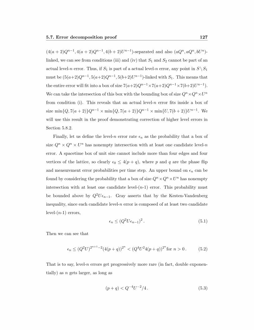
5.7. Error decomposition proof 127
(4(a + 2)Qn−1, 4(a + 2)Qn−1, 4(b + 2)Un−1)-separated and also (aQn, aQn, bUn)-
linked, we can see from conditions (iii) and (iv) that S1 and S2 cannot be part of an
actual level-n error. Thus, if S1 is part of a actual level-n error, any point in S \S1
must be (5(a+2)Qn−1, 5(a+2)Qn−1, 5(b+2)Un−1)-linked with S1. This means that
the entire error will fit into a box of size 7(a+2)Qn−1×7(a+2)Qn−1×7(b+2)Un−1).
We can take the intersection of this box with the bounding box of size Qn×Qn×Un
from condition (i). This reveals that an actual level-n error fits inside a box of
size minQ, 7(a + 2)Qn−1 ×minQ, 7(a + 2)Qn−1 ×minU, 7(b + 2)Un−1. We
will use this result in the proof demonstrating correction of higher level errors in
Section 5.8.2.
Finally, let us define the level-n error rate εn as the probability that a box of
size Qn ×Qn × Un has nonempty intersection with at least one candidate level-n
error. A spacetime box of unit size cannot include more than four edges and four
vertices of the lattice, so clearly ε0 ≤ 4(p + q), where p and q are the phase flip
and measurement error probabilities per time step. An upper bound on εn can be
found by considering the probability that a box of size Qn×Qn×Un has nonempty
intersection with at least one candidate level-(n-1) error. This probability must
be bounded above by Q2Uεn−1. Gray asserts that by the Kesten-Vandenberg
inequality, since each candidate level-n error is composed of at least two candidate
level-(n-1) errors,
εn ≤ (Q2Uεn−1)2 . (5.1)
Then we can see that
εn ≤ (Q2U)2n+1−2(4(p+ q))2
n< (Q4U24(p+ q))2
nfor n > 0 . (5.2)
That is to say, level-n errors get progressively more rare (in fact, double exponen-
tially) as n gets larger, as long as
(p+ q) < Q−4U−2/4 . (5.3)

5.8. Lower bound on accuracy threshold 128
Now, Gray further asserts that a simple Borel-Cantelli argument shows that given
this condition, with probability 1 every error belongs to an actual level-n error for
some n ≥ 0.
5.8 Lower bound on accuracy threshold
5.8.1 Correction of level-0 errors
Any actual level-0 error (a set of only phase flip errors or only measurement errors
fitting inside a 2 × 2 × 1 spacetime box and (a, a, b)-separated from any other
errors) get corrected automatically by the basic local rules (as laid out in Section
5.6). We can demonstrate this explicitly for several examples in figures 5.1 and
5.2. In the selected examples, we assume that these sites (denoted by black circles
in the figures) are located in the southwest quadrant of a colony. (Errors located
elsewhere in the colony would be handled similarly.) In the third example of Figure
5.1, the southwest site inside the dotted box decides to flip the qubit to its north
in the first update, and the northwest site then flips the qubit to its east in the
second update, which closes the chain of errors. In the fourth example of Figure
5.2, the southwest site flips the qubit to its east in the first time step, while all
other sites do nothing, and during the second time step these actions are repeated.
Note that a trivial loop of flips is a stabilizer operator of the toric code, and thus
acts as the identity on the encoded qubits.
By exhausting over all possible configurations of actual level-0 errors, we see
that they are always corrected within two time steps, provided that a ≥ 2 and
b ≥ 2 (so as to be sufficiently isolated from any other noise).
5.8.2 Correction of higher level errors
An actual level-1 error fits inside a spacetime box of size Q × Q × U . It may be
contained inside a single colony, or at worst, it is contained within a 2×2 grouping

5.8. Lower bound on accuracy threshold 129
M U M U
M
M
U
U
M
M
M MU U
U
U
M MU U
M MU U
Figure 5.1: Examples of level-0 flip errors being corrected. The leftmost diagram
in each row contains a distinct level-0 error. The blue lines are bit flip or phase flip
errors. The red squares are sites with a nontrivial syndrome measurement. The
green arrows are controlled flips based on the local update rules. Measurement
and update steps are denoted by M and U.
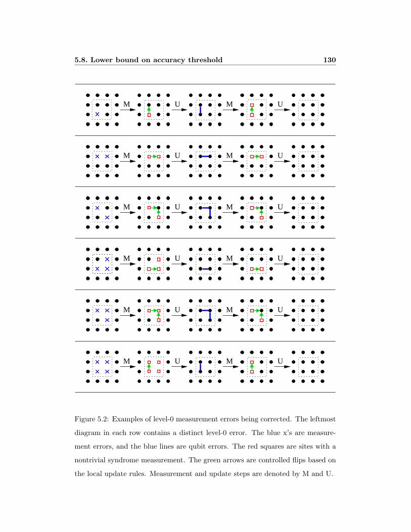
5.8. Lower bound on accuracy threshold 130
M U M U
M
M
U
U
M
M
M MU U
U
U
M MU U
M MU U
Figure 5.2: Examples of level-0 measurement errors being corrected. The leftmost
diagram in each row contains a distinct level-0 error. The blue x’s are measure-
ment errors, and the blue lines are qubit errors. The red squares are sites with a
nontrivial syndrome measurement. The green arrows are controlled flips based on
the local update rules. Measurement and update steps are denoted by M and U.

5.8. Lower bound on accuracy threshold 131
of colonies. Any level-1 error (or higher-level error) that is completely contained
within a single colony will be corrected in a straightforward manner by the basic
local rules (Section 5.6). The two endpoints of such an error chain would drift
toward the center of the colony, where they will meet up and form a trivial loop.
Error chains across colonies, however, require more sophisticated processing.
We will show in the following argument that any actual level-n error will be cor-
rected within 3Un time steps, and that it will always be contained inside a space
of 2Qn × 2Qn. Since actual level-n errors are (aQn, aQn, bUn)-separated from one
another, they will always get corrected before another one occurs (provided a ≥ 2
and b ≥ 3).
Suppose a level-1 error occurs that stretches across neighboring colonies. At
the end of the current work period, let xC and xN be the computed syndromes
(according to the Count field) at one of the affected colonies of itself and of its
neighbor. There are four possible values for xC and xN , depending on at what
point during the work period the ends of the error chain migrated to the centers of
each colony, and also depending on how the colony centers were affected by level-0
noise. If xC is zero (off), then this colony will do nothing. If both xC and xN are
one (on), then the colony will make the proper decision to deal with this error by
following the basic rules in Section 5.6 (based on the computed syndromes instead
of its local neighborhood). The only dangerous case is when xC is on, but xN is
off. The colony may then execute a flip (via FlipSignal) that moves its syndrome
in the wrong direction and thereby increases the size of the level-1 error.
To prevent this last case from ever happening, we want to guarantee that if
a level-1 error occurs with enough time left in the work period for the computed
syndrome of a colony to be on, then the computed syndromes of its neighbors
must be valid. So we will want to set the self-count threshold fC to be as high as
possible and the neighbor-count threshold fN to be as low as possible. However,
if fC is too high, then level-0 noise could prevent a syndrome from ever turning
on in a colony (by temporarily moving a syndrome away from the center), or if
fN is too low, then level-0 noise could masquerade as a higher-level syndrome (by

5.8. Lower bound on accuracy threshold 132
temporarily creating a syndrome at the center of a neighboring colony). Since
actual level-0 errors are (a, a, b)-separated from one another, and since they are
always corrected within two time steps, we could choose
fN =4b, fC =
b− 4b
. (5.4)
Level-0 noise can then never affect the coarse-grained count of higher-level syn-
dromes, because the presence or absence of syndromes at a colony center will never
be changed by more than two during an interval of b time steps. (See the discus-
sion of the Count field in Section 5.5.2.) Note that we could have chosen fNb = 3
and fCb = (b− 3), which would have been sufficient for dealing with level-0 noise,
but we will need the choices of equation (5.4) to deal with higher level noise.
It now remains for us to find a bound on b that will guarantee the neighbor
counts to be valid whenever a colony’s syndrome is on. Near the end of Section
5.7, we derived another bound on the size of an actual level-1 error. In particular,
we found that all of the points in the set of errors differ in time by no more than
7(b + 2) time steps. If our level-1 error was a long chain of errors connecting the
center of one colony to some site in a neighboring colony, the endpoint of the
error chain in the neighboring colony should migrate to its center no later than
7(b + 2) + 2Q time steps after the appearance of a syndrome in the center of the
first colony. It will also take Q time steps for the signal from the neighboring
colony to reach the first colony center.
Suppose that the earliest point in the level-1 error occurs with T time steps
remaining in the current work period. Then whenever
fCb ≤⌈T
b
⌉(5.5)
we require that
fNb ≤⌊T − 7(b+ 2)− 3Q
b
⌋. (5.6)
If we choose a = 2 (which is consistent with all previous bounds on a), then we

5.8. Lower bound on accuracy threshold 133
can choose colony size Q = 4(a+ 2) = 16. We can then rearrange equations (5.4),
(5.5), and (5.6) to read
⌊T
b
⌋≥(
11 +62b
)whenever
⌈T
b
⌉≥ (b− 4) . (5.7)
We can satisfy condition (5.7) for all values of T if we choose b such that
(b− 5) ≥(
11 +62b
). (5.8)
This holds true for b ≥ 20. Previously we wanted U = b2 (for the coarse-grained
count), and we also required U ≥ 4(b + 2) (for the error decomposition proof).
We could choose b = 20, U = 400, or if we prefer working with powers of two, let
b = 32 and U = 1024. In the first case fN = 1− fC = 1/5 and in the second case
fN = 1− fC = 1/8.
Since the same rules are followed for correcting level-1 errors across neighboring
colonies as are responsible for correcting level-0 errors across neighboring cells, we
know that any actual level-1 error will be corrected within two workperiods, once
the syndromes are reported at their colony centers. Depending on the value of
T (the number of time steps remaining in the current work period when a level-
1 error occurs), the computed syndromes may not be on until after a full work
period. Consequently, the worst case for correcting actual level-1 errors requires
no more than 3U time steps.
All of the above reasoning is valid for higher-level errors as well. In particular,
the coarse-grained count was defined in such a way that level-(n-1) noise will not
disrupt the counting of syndromes in a level-n colony. The only noteworthy change
is that for correcting a level-n error, the 3Q term appearing in equation (5.6) gets
replaced by 3Qn
Un−1 , which is strictly less than 3Q (if Q < U), so the bound on b
becomes more relaxed for higher-level errors (eventually approaching b ≥ 17).
Finally, we have a lower bound on the accuracy threshold of our local error
correction scheme. From equation (5.3) and our choices of Q and U , we can
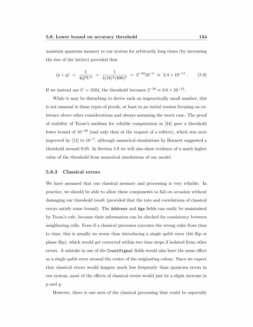
5.8. Lower bound on accuracy threshold 134
maintain quantum memory in our system for arbitrarily long times (by increasing
the size of the lattice) provided that
(p+ q) <1
4Q4U2=
14(16)4(400)2
= 2−2210−4 ≈ 2.4× 10⁻¹¹ . (5.9)
If we instead use U = 1024, the threshold becomes 2−38 ≈ 3.6× 10⁻¹².
While it may be disturbing to derive such an impractically small number, this
is not unusual in these types of proofs, at least in an initial version focusing on ex-
istence above other considerations and always assuming the worst case. The proof
of stability of Toom’s medium for reliable computation in [34] gave a threshold
lower bound of 10−28 (and only then at the request of a referee), which was next
improved by [15] to 10−7, although numerical simulations by Bennett suggested a
threshold around 0.05. In Section 5.9 we will also show evidence of a much higher
value of the threshold from numerical simulations of our model.
5.8.3 Classical errors
We have assumed that our classical memory and processing is very reliable. In
practice, we should be able to allow these components to fail on occasion without
damaging our threshold result (provided that the rate and correlations of classical
errors satisfy some bound). The Address and Age fields can easily be maintained
by Toom’s rule, because their information can be checked for consistency between
neighboring cells. Even if a classical processor executes the wrong rules from time
to time, this is usually no worse than introducing a single qubit error (bit flip or
phase flip), which would get corrected within two time steps if isolated from other
errors. A mistake in one of the CountSignal fields would also have the same effect
as a single qubit error around the center of the originating colony. Since we expect
that classical errors would happen much less frequently than quantum errors in
our system, most of the effects of classical errors would just be a slight increase in
p and q.
However, there is one area of the classical processing that could be especially
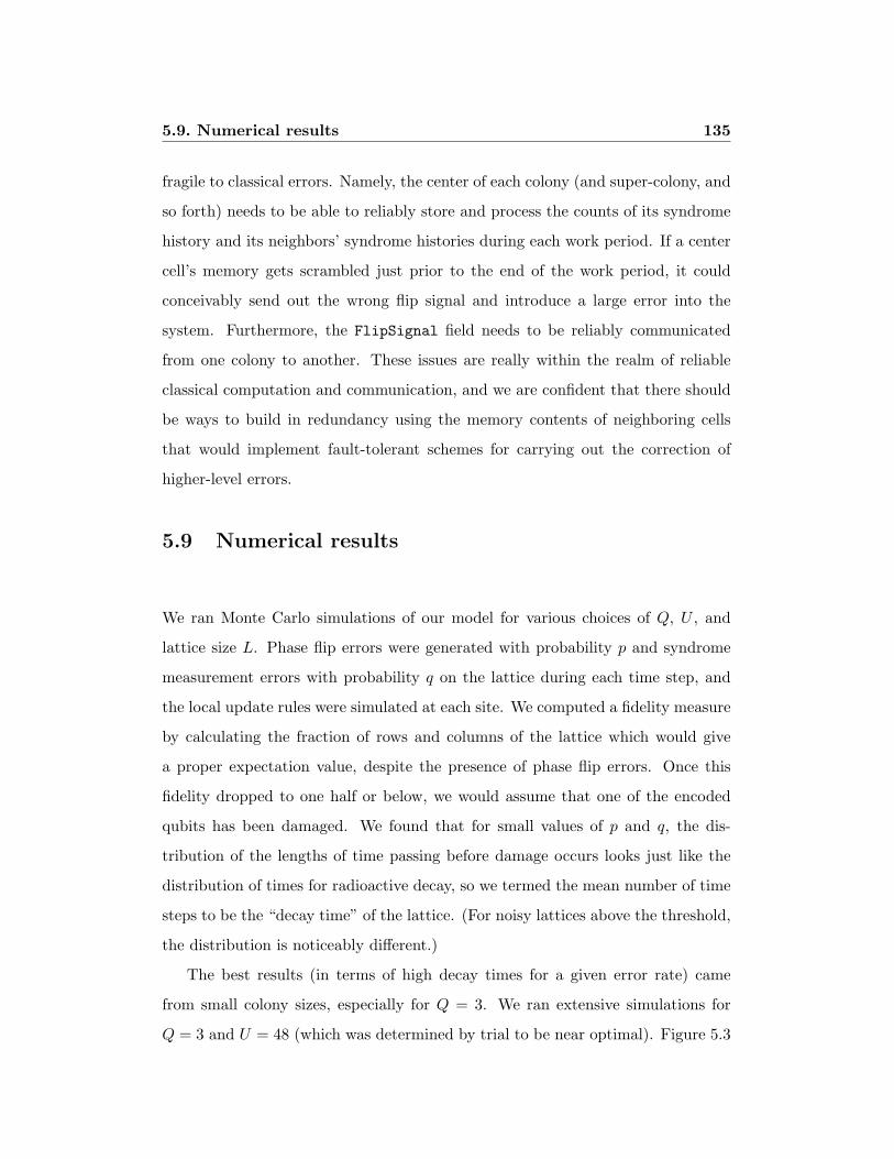
5.9. Numerical results 135
fragile to classical errors. Namely, the center of each colony (and super-colony, and
so forth) needs to be able to reliably store and process the counts of its syndrome
history and its neighbors’ syndrome histories during each work period. If a center
cell’s memory gets scrambled just prior to the end of the work period, it could
conceivably send out the wrong flip signal and introduce a large error into the
system. Furthermore, the FlipSignal field needs to be reliably communicated
from one colony to another. These issues are really within the realm of reliable
classical computation and communication, and we are confident that there should
be ways to build in redundancy using the memory contents of neighboring cells
that would implement fault-tolerant schemes for carrying out the correction of
higher-level errors.
5.9 Numerical results
We ran Monte Carlo simulations of our model for various choices of Q, U , and
lattice size L. Phase flip errors were generated with probability p and syndrome
measurement errors with probability q on the lattice during each time step, and
the local update rules were simulated at each site. We computed a fidelity measure
by calculating the fraction of rows and columns of the lattice which would give
a proper expectation value, despite the presence of phase flip errors. Once this
fidelity dropped to one half or below, we would assume that one of the encoded
qubits has been damaged. We found that for small values of p and q, the dis-
tribution of the lengths of time passing before damage occurs looks just like the
distribution of times for radioactive decay, so we termed the mean number of time
steps to be the “decay time” of the lattice. (For noisy lattices above the threshold,
the distribution is noticeably different.)
The best results (in terms of high decay times for a given error rate) came
from small colony sizes, especially for Q = 3. We ran extensive simulations for
Q = 3 and U = 48 (which was determined by trial to be near optimal). Figure 5.3
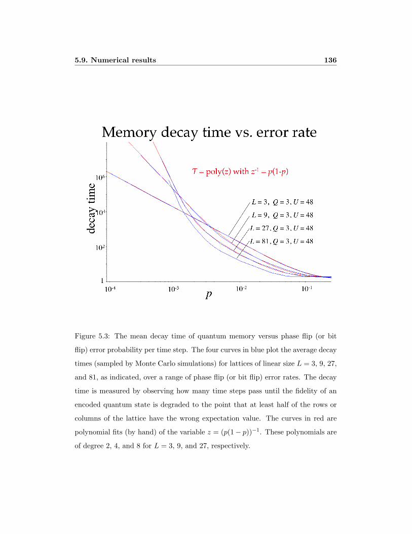
5.9. Numerical results 136
Figure 5.3: The mean decay time of quantum memory versus phase flip (or bit
flip) error probability per time step. The four curves in blue plot the average decay
times (sampled by Monte Carlo simulations) for lattices of linear size L = 3, 9, 27,
and 81, as indicated, over a range of phase flip (or bit flip) error rates. The decay
time is measured by observing how many time steps pass until the fidelity of an
encoded quantum state is degraded to the point that at least half of the rows or
columns of the lattice have the wrong expectation value. The curves in red are
polynomial fits (by hand) of the variable z = (p(1− p))−1. These polynomials are
of degree 2, 4, and 8 for L = 3, 9, and 27, respectively.

5.10. Conclusion 137
displays our numerical simulations of lattices with linear size L = 3, 9, 27, and 81
over a range of error probabilities p, with perfect measurements (q = 0).
Although not shown, it is worth remarking that the plots do not appear to
change much if we allow small measurement errors, such as q < p2. Also, we
observe qualitatively the same behavior of the decay times as a function of q for
the cases p = 0 and p = q.
We have only been able to analytically show the existence of an accuracy
threshold for local control of quantum memory in our model with very large lattice
sizes andQ ≥ 16. However, our numerical results support the suggestion that small
colony sizes (such as Q = 3) also exhibit an accuracy threshold, and that errors
on the order of 10−4 or even 10−3 can be tolerated. The asymptotic slopes of the
curves for L = 3, 9, and 27 can be measured to show that the decay time grows as
T ∝ p−2, T ∝ p−4, and T ∝ p−8, respectively. This is very encouraging because
it supports a double exponential growth in memory storage time as a function of
the number of levels implemented in the lattice. It took too much running time
to sufficiently test L = 81 at low values of p, but the plot appears to be consistent
with T ∝ p−16 around the purported threshold. More generally, we expect based
on these numerical results that the decay time of quantum memory goes as T ∝
p−2kfor p below threshold when k levels of the hierarchy are implemented. If
true, then the required spatial resources scale as O((log T )2) physical qubits and
classical processors with O((log log T )2) memory per processor. The amount of
processing required per time step, however, is independent of the lattice size or
desired memory storage time.
5.10 Conclusion
We make the following observation about designing systems to protect classical
or quantum information. In either a two-dimensional lattice of classical bits or a
four-dimensional toric code protecting quantum bits, there exists a local rule (e.g.,
5.10. Conclusion 138
Toom’s rule) that removes error clusters in a robust manner, because the errors
are two-dimensional surfaces with one-dimensional boundaries. These boundaries
can be eaten away in a preferred direction, so that the size of error clusters will
shrink over time. Provided that the underlying error rate is low enough and that
errors are mostly uncorrelated in space and time, then errors of arbitrary size will
get removed on average before new errors of comparable size are generated. An
accuracy threshold thus exists for local error correction in these systems [82, 2].
There is a further analogy between classical and quantum systems. In a one-
dimensional array of bits, or a two-dimensional toric code of qubits, a cluster of
errors forms a one-dimensional string, with zero-dimensional (point) boundaries.
In these cases, Gacs [33] and this present work show that there exists a local
rule with an accuracy threshold for error correction, although the procedures and
proofs are much more complex than as needed for Toom’s rule. Protecting classical
information in n dimension by purely local controls appears to be comparable (in
terms of the scaling of resources) to protecting information in 2n dimensions.
But do we really need a minimum of two dimensions to robustly store quan-
tum information? Gottesman [37] and Aharonov and Ben-Or [1] argue that there
should exist a one-dimensional stabilizer or polynomial code requiring only local
operations (acting in parallel) and perhaps global (classical) processing of error
syndromes that would possess an accuracy threshold, but no explicit construction
has been given. We have also experimented to some extent with quantum convolu-
tional codes, as described in [69, 70], but they appear to lack a means for correcting
arbitrarily large errors. It still remains open whether a one-dimensional array of
qubits could have an accuracy threshold under some error-correcting scheme that
is local in both quantum and classical processing, although it seems unlikely.
Now that purely local control of quantum information has been demonstrated
in two dimensional structures, there remains great room for improving on the value
of the accuracy threshold. Our lower bound is based on some pessimistic assump-
tions in deriving equation (5.3), and by no means has our protocol been completely
optimized. Our model could also be improved in handling faults in the classical

5.10. Conclusion 139
memory and processing. Additionally, future work could relate our qubit and mea-
surement error probabilities p and q to gate errors and ancilla preparation errors
(which are perhaps more directly connected to an experimental implementation).
Kuperberg [50] has suggested that there may be a sequence of local error-
correcting schemes of toric codes with progressively larger neighborhoods whose
accuracy thresholds would transition from those reported in this work up to a few
percent, as achieved by the global error syndrome processing scheme described
in Section 4.5. It would be interesting to determine what would be good choices
for local rules with larger neighborhoods that could quickly correct a larger set of
level-0 errors.

140
Appendix A
Translation of Bavard’s “Hyperbolic families
of symplectic lattices” [8]
A.1 Introduction
A symplectic lattice in a complex Hermetian postive definite vector space (V,H) is
a lattice Λ of V which admits a symplectic basis for ImH. For example, the period
lattice of a manifold of genus ≥ 1 is a symplectic lattice for the Riemann form.
The symplectic lattices Λ in complex dimension g ≥ 1 correspond to principally
polarized abelian varieties V/Λ and are thus parameters for Siegel’s space Hg.
The study of Hermite’s constant µ of symplectic lattices (defined by µ(Λ) =
infH(λ, λ) for λ ∈ Λ\0) was approached in [B-S] and followed in [B-M1] and
[Bv]. The maximal value of µ on Hg, which is the analog of the classical Hermite’s
constant, is not known except for g = 1, 2 or 4 for the usual theory. One is inter-
ested in the lattices which realize a local maximum of µ on Hg, or extremal lattices
in the symplectic sense. These lattices are characterized in [B-M1]; however, the
known examples of such lattices are very few and, with a lone exception (JW , see
below), are already extremal in the usual sense (D4, E8, Leech’s lattice Λ24, . . .).
We study here the symplectic lattice families that present a two-fold interest.
Firstly, they provide new examples of extremal symplectic lattices which gener-

A.1. Introduction 141
ally are not extremal in the usual sense. The extremal symplectic lattices are a
particular case of perfect symplectic lattices (see Section A.2.4). We obtain many
examples of perfect symplectic lattices (300 with g ≤ 6) among which we find
certain traditional lattices: D4, E8, K12, Λ16, Λ24; we also describe several exten-
sions of extremal symplectic lattices. In small dimensions, we find in particular
a new extremal point of H3 and five new perfect points of H4 of which three are
extremal. Secondly, these families permit the testing of the general counting pro-
posed in [Bv]. We establish for each one of them a complete theory analogous
to classical lattice theory: Voronoı’s theorem (Proposition A.2.3), Voronoı’s algo-
rithm (Proposition A.2.10), Morse’s theory (Proposition A.2.13). These hyperbolic
families are defined as follows. Let H be the Poincare half plane and let M be a
symmetric real positive definite g × g matrix. We define
HM = zM ; z ∈ H ⊂ Hg. (∗)
The family HM is a completely geodesic subvariety of Siegel’s space Hg, isometric
(up to a factor) to H provided by the Poincare metric (Section A.2.1), which
justifies the adjective “hyperbolic.”
Hermite’s constant defines by restriction on HM two dual geodesic tilings of the
hyperbolic plane (Figure A.3), of the types Dirichlet-Voronoı (DVM ) and Delaunay
(DelM ), and there is a supplementary dictionary between these tilings and the
relative properties with HM of corresponding lattices (for example, perfection and
relative eutaxy: see Theorem A.2.1). The vertices of DVM are the perfect points
of the family, while the vertices of DelM , called principal points, are naturally
bound to a geometric interpretation of length functions (Proposition A.2.2). On
this point the theory of hyperbolic families presents two new phenomena compared
to the case of classical lattices. Firstly, certain principal points belong here to the
parameter space H whereas for the lattices they are all situated at infinity (see
[Bv, section 1.3]). Secondly, we present the notion of principal length functions:
they are the length functions necessary for describing the situation and, contrary
A.1. Introduction 142
to the lattice case, they do not coincide with the functions that realize Hermite’s
constant (see section A.2.5).
The search for examples is guided by the following idea: if the matrix M
is rather “interesting” (for example, if M and its inverse have many minimal
vectors), the family (*) has some chance of containing marked points. One will
find in Section A.3.6 a remarkable family which alone contains 16 (non-isomorphic)
perfect symplectic lattices of H8. The fact that the space of parameters H is of small
dimension and of a very familiar geometry renders the determination of interesting
points of HM particularly simple to put into practice. In certain cases one can
even connect the relative properties with the global properties. Thus when M has
a sufficient number of automorphisms, the relative eutaxy with HM (which tests
itself in dimension 2) is equivalent to the ordinary eutaxy (Proposition A.2.6).
When M is rational, the family (*) admits a complete symplectic action of
a subgroup congruent to PSL(2,Z). We study the behavior of µ|HM near the
points (Proposition A.2.11) and we establish a definitive result (Corollary A.2.12)
like that of two of Euler’s formulas (A.2.32), (A.2.36) and a mass formula (A.2.33).
A particularly interesting case is M = An. We give here a more complete descrip-
tion (part 2) which leads to 3 extensions F2n, G2n, J2n and a family H2n(ϕ)
(ϕ ∈ SL(2,Z)) of extremal lattices (in the symplectic sense only for F2n, J2n and
H2n(ϕ)). The group which acts on the situation is Γ0(n+1), and at the same time
the number of marked points of the augmented family is the index of Γ0(n+ 1) in
PSL(2,Z).
The complex dimension 3 merits some commentary. The lattice F6 is a new
example of an extremal point in H3. Two other extremal points were known
previously: the Jacobian JK of the Klein manifold K (or the lattice A(2)6 ) which
is one of the six extremal lattices of real dimension 6, and the Jacobian JW of the
exceptional Wiman manifold W . The situation therefore appears to be analogous
to that of Riemann surfaces of genus 3. In [Sc], P. Schmutz exhibits three local
maxima of the systole in genus 3: K, W and a less remarkable surface of which
the Jacobian seems to correspond to F6. In terms of numeric values of µ, we have
A.2. General study of hyperbolic families 143
µ(JW ) = 1 + 1/√
3 ' 1.5773 and we remark that µ(F6) = 6/√
15 ' 1.5491 is
also larger than µ(JK) = 4/√
7 ' 1.5118, the value presented in [B-S] as a global
maximum of µ on H3.
Acknowledgements. I thank Anne-Marie Berge for her remarks on a first version
of this article that was presented at the Luminy conference on lattices (September
1996). I also thank Christian Batut for initiating me in the PARI system of
calculation and furthermore thank the other authors of PARI for their availability.
A.2 General study of hyperbolic families
Notations. If M is a matrix, we will denote M ′ as its transpose.
For a square m×m matrix A and u ∈ Rm we define A[u] = u′Au.
We denote Sm(R) (resp. Sm(C)) as the space of symmetric m × m matrices
with real (resp. complex) coefficients, I as the identity matrix, J =(
0 I−I 0
)and
〈u, v〉 = u′v (u, v ∈ Rm) as the usual Euclidean scalar product.
A.2.1 Symplectic lattices and hyperbolic families
The lattices of the usual Euclidean space of dimension m (m ≥ 1) will be here
parameters, via the Gram matrices, for the symmetric space Pm of real positive
m × m matrices with determinant 1. One has a correspondance between the
matrices A = PP ′ of Pm (P ∈ SL(m,R)) and the marked lattices (i.e., provided
with a basis) Λ = P ′Zm considered except for direct isometry. Length functions
are defined on Pm by
lu(A) = A[u] (A ∈ Pm, u ∈ Rm). (A.2.1)
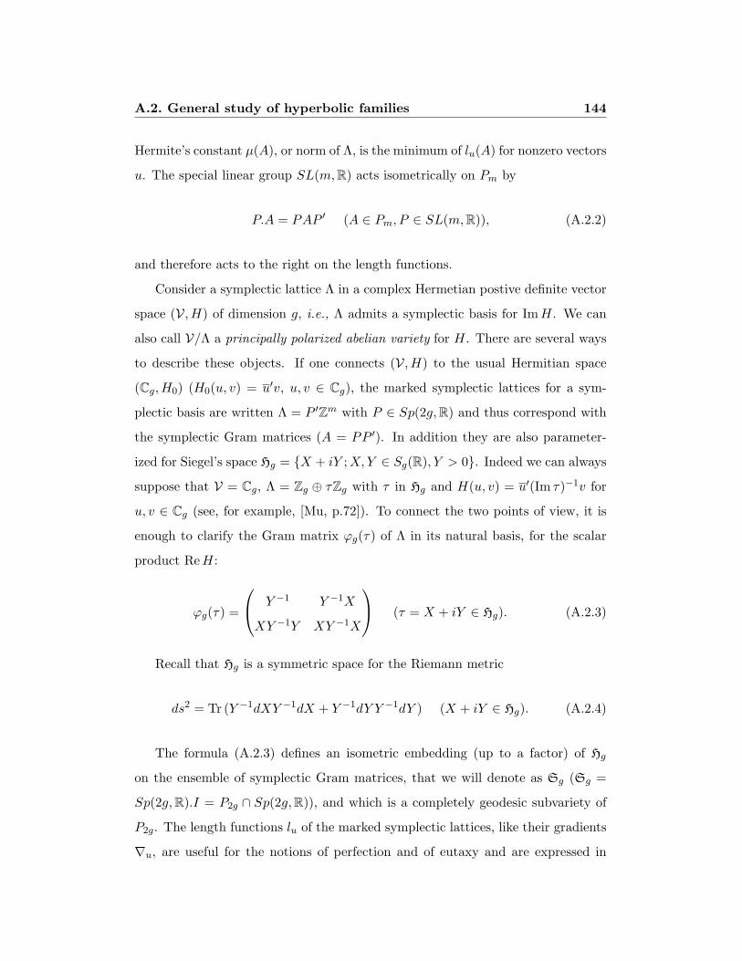
A.2. General study of hyperbolic families 144
Hermite’s constant µ(A), or norm of Λ, is the minimum of lu(A) for nonzero vectors
u. The special linear group SL(m,R) acts isometrically on Pm by
P.A = PAP ′ (A ∈ Pm, P ∈ SL(m,R)), (A.2.2)
and therefore acts to the right on the length functions.
Consider a symplectic lattice Λ in a complex Hermetian postive definite vector
space (V,H) of dimension g, i.e., Λ admits a symplectic basis for ImH. We can
also call V/Λ a principally polarized abelian variety for H. There are several ways
to describe these objects. If one connects (V,H) to the usual Hermitian space
(Cg,H0) (H0(u, v) = u′v, u, v ∈ Cg), the marked symplectic lattices for a sym-
plectic basis are written Λ = P ′Zm with P ∈ Sp(2g,R) and thus correspond with
the symplectic Gram matrices (A = PP ′). In addition they are also parameter-
ized for Siegel’s space Hg = X + iY ;X,Y ∈ Sg(R), Y > 0. Indeed we can always
suppose that V = Cg, Λ = Zg ⊕ τZg with τ in Hg and H(u, v) = u′(Im τ)−1v for
u, v ∈ Cg (see, for example, [Mu, p.72]). To connect the two points of view, it is
enough to clarify the Gram matrix ϕg(τ) of Λ in its natural basis, for the scalar
product ReH:
ϕg(τ) =
Y −1 Y −1X
XY −1Y XY −1X
(τ = X + iY ∈ Hg). (A.2.3)
Recall that Hg is a symmetric space for the Riemann metric
ds2 = Tr (Y −1dXY −1dX + Y −1dY Y −1dY ) (X + iY ∈ Hg). (A.2.4)
The formula (A.2.3) defines an isometric embedding (up to a factor) of Hg
on the ensemble of symplectic Gram matrices, that we will denote as Sg (Sg =
Sp(2g,R).I = P2g ∩ Sp(2g,R)), and which is a completely geodesic subvariety of
P2g. The length functions lu of the marked symplectic lattices, like their gradients
∇u, are useful for the notions of perfection and of eutaxy and are expressed in

A.2. General study of hyperbolic families 145
Siegel’s space by the following formulas (see [Bv]):
lu(τ) = Y −1[a+Xb] + Y [b]
∇u(τ) = −i(a+ τb)(a+ τb)′(τ = X + iY ∈ Hg, u =
ab
∈ R2g). (A.2.5)
With each element M of Pg we associate a hyperbolic family parameterized by
the Poincare half plane H:
HM = zM ; z ∈ H . (A.2.6)
The intersection W of hyperbolic families is a subvariety of Hg with dimension
g(g + 1)/2 + 1. The metric induced on W at the point zM is written as
g (|dz|/Im z)2 + (|z|/Im z)2 Tr(M−1dM
)2, (A.2.7)
so that the two natural coverings carried by W (defined by the product structure
H × Pg) are orthogonal. The hyperbolic families are all isometric with the same
homothetic of H, and they are completely geodesic. Recall that if Q is a Lie
subgroup related to SL(n,R), stable under transposition, then Q.I is completely
geodesic in Pn (see [Eb, p.131]). However, ϕg(HI) is of the form Q.I with
Q =
δI γI
βI αI
;α, β, γ, δ ∈ R, αδ − βγ = 1
. (A.2.8)
When M = PP ′ is unspecified, we see that HM =(
P 00 P ′−1
).HI is an isometric
image of HI. In the orthogonal covering, zPg = zM ;M ∈ Pg is completely
geodesic for Re z = 0 (by a similar argument) and only in this case.
Remark A.2.1. (1) In the following we will study the families HM where M has
an unspecified positive determinant. We can restrict ourselves to the case of de-
terminant 1 by way of an isometry in the parameter space H.
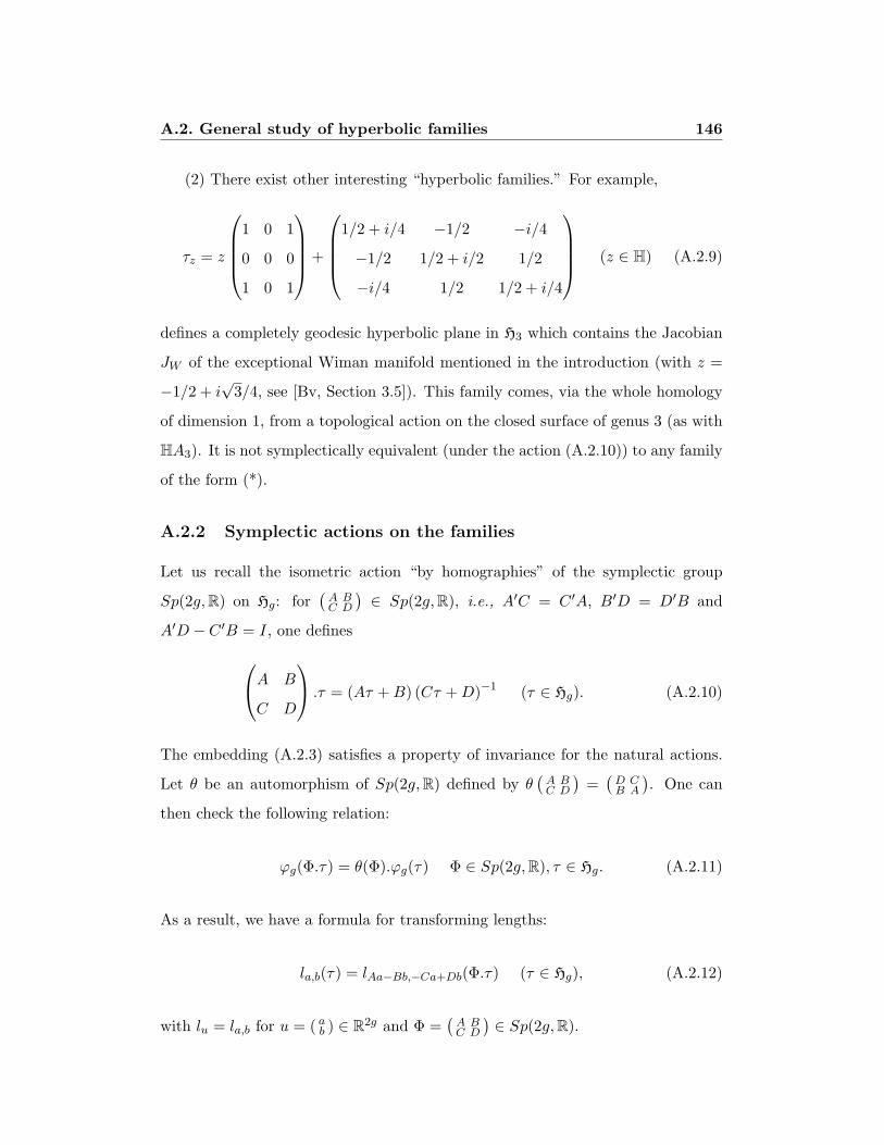
A.2. General study of hyperbolic families 146
(2) There exist other interesting “hyperbolic families.” For example,
τz = z
1 0 1
0 0 0
1 0 1
+
1/2 + i/4 −1/2 −i/4
−1/2 1/2 + i/2 1/2
−i/4 1/2 1/2 + i/4
(z ∈ H) (A.2.9)
defines a completely geodesic hyperbolic plane in H3 which contains the Jacobian
JW of the exceptional Wiman manifold mentioned in the introduction (with z =
−1/2 + i√
3/4, see [Bv, Section 3.5]). This family comes, via the whole homology
of dimension 1, from a topological action on the closed surface of genus 3 (as with
HA3). It is not symplectically equivalent (under the action (A.2.10)) to any family
of the form (*).
A.2.2 Symplectic actions on the families
Let us recall the isometric action “by homographies” of the symplectic group
Sp(2g,R) on Hg: for(
A BC D
)∈ Sp(2g,R), i.e., A′C = C ′A, B′D = D′B and
A′D − C ′B = I, one defines
A B
C D
.τ = (Aτ +B) (Cτ +D)−1 (τ ∈ Hg). (A.2.10)
The embedding (A.2.3) satisfies a property of invariance for the natural actions.
Let θ be an automorphism of Sp(2g,R) defined by θ(
A BC D
)=(
D CB A
). One can
then check the following relation:
ϕg(Φ.τ) = θ(Φ).ϕg(τ) Φ ∈ Sp(2g,R), τ ∈ Hg. (A.2.11)
As a result, we have a formula for transforming lengths:
la,b(τ) = lAa−Bb,−Ca+Db(Φ.τ) (τ ∈ Hg), (A.2.12)
with lu = la,b for u = ( ab ) ∈ R2g and Φ =
(A BC D
)∈ Sp(2g,R).

A.2. General study of hyperbolic families 147
We will call the group of automorphisms of the family HM the subgroup of
Sp(2g,Z) which fixes HM point by point, denoted Aut(HM).
Proposition A.2.1. (1) The group of automorphisms of HM is isomorphic to
the group of automorphisms of M .
(2) The family HM is symplectically equivalent to the family HM−1.
Proof. (1) One can quickly verify that all automorphisms of HM are of the form(P 00 P ′−1
)with P ∈ GL(g,Z) and PMP ′ = M , i.e., P ∈ Aut(M); the isomorphisms
are then evident.
(2) The families HM and HM−1 are exchanged by a complete symplectic trans-
formation: 0 I
−I 0
.zM = −1zM−1. (A.2.13)
In addition, each family HM admits a symplectic action of PSL(2,R):
αI βM
γM−1 δI
.zM =αz + β
γz + δM (α, β, γ, δ ∈ R, αδ − βγ = 1), (A.2.14)
which induces the usual action of PSL(2,R) on the plane of parameters H. When
M is rational, we thus have a complete symplectic action of a subgroup of finite
index Γ ⊂ PSL(2,Z) and we can restrict our study to a fundamental domain of Γ
in H. Let m ∈ N∗ such that mM and mM−1 are complete: one takes Γ = Γ(m)
to be the subgroup of principal congruence (Γ = PSL(2,Z) if M has determinant
1). But one can often choose Γ to contain Γ(m): for example, HAn (resp. HDn)
admits a complete symplectic action of the group Γ0(n+ 1) (resp. Γ0(4)) with
Γ0(m) =
α β
γ δ
∈ PSL(2,Z); γ ≡ 0(m)
. (A.2.15)
The fixed points of Γ are in general interesting because they have more automor-
phisms than a “generic” point of the family (examples: 1+i2 D2n, 1+i
2 D4 ' 2+i5 A4 '
E8, 5+i√
314 A6 ' K12, 5+i
13 A(2)12 ' Λ24, . . .).
A.2. General study of hyperbolic families 148
There is a also a symmetry coming from the anti-symplectic action of Φ0 =(−I 00 I
)on P2g which fixes Sg. In Hg, the action is written Φ0.τ = −τ (τ ∈
Hg); it fixes each hyperbolic family and respects the length function gradients:
∇u(Φ0.τ) = Φ0(∇Φ′0u(τ)) (τ ∈ Hg, u ∈ R2g). The forms ϕg(τ) and ϕg(−τ)
(GL(2g,Z) equivalent) therefore have the same symplectic nature.
Remark A.2.2. If P ∈ GL(g,Z), the families HM and H(PMP ′) are exchanged
by a complete symplectic transformation which induces the identity on H. The
symplectic nature of zM therefore does not depend upon the specific lattice used
to define M .
A.2.3 Geometric study of lengths
With the postive definite matrix M being fixed, we study the length functions
and Hermite’s constant restricted to the family HM , such as functions on the
parameter space H. We therefore define
µM (z) = µ(zM) (z ∈ H), (A.2.16)
and lMu (z) = lu(zM) with u = ( ab ) a nonzero vector of R2g. We also define
∆Mu = M−1[a]M [b]− 〈a, b〉2 and zM
u =−〈a, b〉+ i
√∆M
u
M [b](A.2.17)
(with zMu = ∞ if M [b] = 0). We observe that ∆M
u ≥ 0 from (A.3.3). The point
zMu is in H if ∆M
u > 0 and in R∪ ∞ = ∂H (the boundary of H) if ∆Mu = 0. It is
the point of H ∪ ∂H which zeroes the gradient of lMu (see (A.2.21)).
One notes that d is the hyperbolic distance in H and hp is the Busemann
function associated with a point at infinity p ∈ ∂H, normalized for hp(i) = 0.
Proposition A.2.2. The length function lMu is expressed geometrically by
lMu = 2√
∆Mu cosh(d(., zM
u )) if zMu ∈ H,
lMu = (M−1[a] +M [b]) exp(hzMu
) if zMu ∈ ∂H
(z ∈ H).

A.2. General study of hyperbolic families 149
Consequently, if zMu ∈ H (resp. zM
u ∈ ∂H), the level curves of lMu are hyperbolic
circles (resp. horocycles) centered at zMu , and their gradient lines are, for close
parameters, the half-geodesic (resp. geodesic) exits of zMu .
Proof. Recall that lMu (z) = (M−1[a] + 2x〈a, b〉+ |z|2M [b])y−1 for z = x+ iy ∈ H.
Hyperbolic distance is given by
cosh(d(z, w)) =|z − w|2 + |z − w|2
|z − w|2 − |z − w|2(z, w ∈ H), (A.2.18)
Also, recall the expression of Busemann functions:
hp(z) = log|z − p|2
Im z(1 + p2)h∞(z) = log
1Im z
(p ∈ R, z ∈ H). (A.2.19)
The verification of the formulas is then elementary.
Proposition A.2.2 also shows that the length functions are strictly convex on the
hyperbolic families. The condition (C) is therefore verified (see [Bv, 2.2 Example
2]) and one has the relative Voronoı’s theorem.
Proposition A.2.3. A point zM is extremal in the family HM if and only if it
is relatively perfect and relatively eutactic.
We note also that the extremal points in HM are isolated in HM ([Bv, Propo-
sition 2.4]). Here is another consequence of Proposition A.2.2: if γ is a geodesic
of H, the function lMu γ is proper (lim|t|→∞ lMu γ(t) =∞) except if zMu is one of
the points at infinity on γ.
Proposition A.2.4. Let u and v be two nonzero vectors of R2g and let k be a
positive real number. Then the ensemble of points z of H such that lMu (z) = klMv (z),
if it is nonempty, is a geodesic which crosses orthogonally the geodesic joining the
points zMu and zM
v (assumed to be distinct).
Proof. One works with the model of the hyperboloid and the associated projec-
tive model. The space S2(R) of real symmetric 2 × 2 matrices is provided by

A.2. General study of hyperbolic families 150
the quadratic form q(A) = −det(A) of signature (2,1). The hyperbolic plane
corresponds to the projection of the negative cone of q (cone of defined ma-
trices): the matrix A =(
U VV W
)with det(A) > 0 is associated with the point
U−1(V + i[det(A)]1/2) of H; this identification is consistent with (A.2.3). The
length functions are defined by linear forms on S2(R):
lMu (A) = −2B(A,ZMu ) with ZM
u =
M [b] −〈a, b〉
−〈a, b〉 M−1[a]
, (A.2.20)
where B indicates the polar bilinear form of q and u = ( ab ) ∈ R2g. The matrix
ZMu is associated with the point zM
u defined by (A.2.17). Suppose that ZMu is not
colinear with ZMv . The equation lMu (A) = klMv (A) therefore defines a projective
line Dk, and when k varies all these projections pass by the polar point (compared
to q) of the projective line ZMu ZM
v , and this point is in the projection of the positive
cone of q. Depending on whether or not Dk crosses the projection of the negative
cone of q, the sought ensemble of z ∈ H is a geodesic orthogonal to the geodesic
joining zMu and zM
v , or it is empty.
We could also write the equations in H: the ensemble of z satisfying lMu (z) =
klMv (z) is a geodesic (if it is nonempty), and orthogonality with the geodesic zMu zM
v
is verified by an elementary calculation.
A.2.4 Relative eutaxy
Let us briefly recall the general definitions of perfection and eutaxy, which are
equivalent to the usual definitions in the classical case (see [Bv, Section 2.1]). Let
V be a Riemann variety provided by a system of length functions (fs)s∈C with
action on a discrete group Π of isometries of V . For all x ∈ V , we denote Sx as
the ensemble (assumed to be finite) of elements of C of minimal length in x. A
point x ∈ V is eutactic (resp. semi-eutactic, resp. weakly eutactic ) if the gradients
Xs(x) = ∇fs(x) (s ∈ Sx) satisfy the relation∑
s∈SxλsXs(x) = 0 with coefficients
λs strictly positive (resp. nonnegative and summing to one, resp. summing to one).
A.2. General study of hyperbolic families 151
We say that x ∈ V is perfect if Xs(x) (s ∈ Sx) affinely generates the tangent space
TxV . For example, we can take V = Pn, C = Zn, Π = SL(2,Z) for the lattices
and V = Hg, C = Z2g, Π = Sp(2g,Z) for the symplectic lattices (with the usual
lengths).
By projecting the gradients orthogonally, these notions can be extended to
relative ones of a vector subspace TxV . For a subvariety W , relative perfection
and eutaxy of TxW coincide with the notions of perfection and eutaxy defined in
W with the induced length functions.
The stabilizer of a point x ∈ V by the action of Γ is called the group of
automorphisms of x and denoted as Aut(x). When Aut(x) is rather rich, one can
reduce the verification of global eutaxy to verification of eutaxy in a subspace of
smaller dimension according to the following remark.
Proposition A.2.5. Let G be a subgroup of Aut(x) and let (TxV )G be the subspace
of fixed points of G in TxV (x ∈ V ). Let F be a vector subspace of TxV which
contains (TxV )G. Then x is eutactic (resp. semi-eutactic, resp. weakly eutactic)
in V if and only if x is eutactic (resp. semi-eutactic, resp. weakly eutactic) relative
to F .
Proof. We must verify that eutaxy in F involves global eutaxy (the inverse being
evident by projection), and we can assume that F = (TxV )G. Let pF be the or-
thogonal projection on F . We observe that the ensemble (Xs)s∈Sx of gradients in x
is stabilized by G and that pF (X) is the average of g.X for g ∈ G (x ∈ TxV ). Con-
sequently, every relation of eutaxy (resp. semi-eutaxy, resp. weak eutaxy) binding
the pF (Xs) implies an analagous relation between the Xs.
Let us return to the study of hyperbolic families.
Proposition A.2.6. Let M ∈ Pg be such that the action of Aut(M) on Rg is
irreducible. Then for all z ∈ H:
(1) zM is eutactic in Hg if and only if zM is eutactic in HM . Suppose also that
Aut(M) contains an element of determinant -1 (which is always the case if g is
A.2. General study of hyperbolic families 152
odd). Then:
(2) ϕg(zM) is eutactic in P2g if and only if zM is eutactic in HM ,
(3) the relative weakly eutactic points (for example, perfect) in HM are insulated
in P2g.
The statements (1) and (2) hold true when replacing eutactic with semi-eutactic
or weakly eutactic.
Lemma A.2.7. Let H be a subgroup of GL(n,R) for which the action on Rn is
irreducible, and let M ∈ Pn be fixed under H (i.e., PMP ′ = M for all P ∈ H).
Then every symmetric matrix fixed under H is a multiple of M ; in particular, M
is the unique point in Pn fixed under H. Furthermore, if n is even, H contains an
element with negative determinant. Then every matrix fixed under H is a multiple
of M .
Proof of the proposition. The assertion (3) can be derived from (2) and the theo-
rem of finitude of weakly eutactic lattices ([B-M2, Theorem 3-5]). It remains then
to prove (1) and (2). The group G = θ(AutHM) (elements of the lattice(
P ′−1 00 P
)with P ∈ Aut(M)) fixes A = ϕg(zM) and TASg (G is included in Sp(2g,R)). As
in the first part of the lemma, the vector space fixed in TASg corresponds via ϕg
to the complex line generated for M , i.e., precisely to the tangent space of the
family HM at the point zM . Then assertion (1) results by way of Proposition
A.2.5.
Now let X =(
U VV ′ W
)∈ TAP2g (where U and W are symmetric) be fixed
under G. We then have P ′−1UP−1 = U (from where PMUMP ′ = MUM),
PV ′P−1 = V ′ (from where PMV P ′ = MV ) and PWP ′ = W for all P ∈ Aut(M).
Applying the lemma leads to U = αM−1, W = βM and (knowing that if g is
even, Aut(M) is not included in SL(g,Z)) V = λI with α, β, λ ∈ R. Moreover, if
X is orthogonal to TASg, i.e., XJA − AJX = 0 and Tr (A−1X) = 0, it is easy
to see that α = β = λ = 0 (X = 0), which completes the proof of the proposition
(Proposition A.2.6). Note that the set of fixed points under G in P2g is reduced
to the hyperbolic family ϕg(HM).

A.2. General study of hyperbolic families 153
Proof of the lemma. Let Y be a matrix that is invariant under H. The ensemble
K of matrices commuting with all the elements of H is a field (Schur’s lemma);
therefore K is isomorphic to R or it contains an element which squares to −I (so
it has complex structure). This last possibility is excluded if n is odd or if H
contains an element with negative determinant. In this case Y is a multiple of M
(YM−1 ∈ K = RI).
Suppose now that H is unspecified but Y is symmetric, and let M = QQ′(Q ∈
SL(n,R)). Then Z = Q−1Y Q′−1 is symmetric and commutes with all the elements
of Q−1HQ. Following the proof of Schur’s lemma (and noting that Z admits a
proper value), one has Z = λI (λ ∈ R), i.e., Y = λM .
For the M that pass the hypotheses of Proposition A.2.6, one will be able to
test global eutaxy in P2g while restricting the family HM to dimension 2 only.
The orthogonal projection on the complex line CM of the gradient of the length
function la,b is equal to 1gTr (M−1∇a,b(zM))M . Consequently the gradient ∇M
a,b(z)
of lMa,b for the Poincare metric is given by (see (A.2.7)):
i∇Ma,b(z) = M−1[a] + 2z〈a, b〉+ z2M [b]. (A.2.21)
A.2.5 Principal length functions. Principal points
We introduce now the notion of a principal length function, which will allow us to
describe µM via a geometric interpretation of Section A.2.3. Contrary to the case
of classical lattices, the ensemble of these functions do not coincide in general with
the ensemble of functions which realize the minimum µM (see the examples and
Remark 1.4 below).
The length function lMa,b depends only on M−1[a],M [b] and 〈a, b〉, and it often
happens that associated length functions of distinct vectors coincide. In the fol-
lowing we consider the ensemble LM of length functions. Note that the point zMu
associated with f = lMu ∈ LM for (A.2.17) depends only on f and will be denoted
zMf or simply zf . It is very easy to compare length functions:

A.2. General study of hyperbolic families 154
Lemma A.2.8. (of comparison) Let γ be a geodesic of H parameterized by ar-
clength, and let ϕ = lMu γ and ψ = lMv γ.
(1) If ϕ(0) = ψ(0) and ϕ′(0) = ψ′(0) then ϕ = ψ.
(2) If ϕ(0) = ψ(0) and ϕ′(0) > ψ′(0) then ϕ(t)− ψ(t) has the same sign as t.
(3) If ϕ and ψ are equal at two distinct points of γ, they coincide.
(4) Let z1, z2 ∈ H. If µM (zi) = lMu (zi) (i = 1, 2), then for all points z pertaining
to the geodesic segment [z1, z2] one has µM (z) = lMu (z).
Proof. One can map γ(t) to exp(t)i for an element of PSL(2,R); thanks to (A.2.12)
one sees that
lMu γ(t) = M−1[c] exp(−t) +M [d] exp(t) (A.2.22)
with suitable (c, d) 6= (0, 0). The assertions (1) and (2) result immediately from
(A.2.22), (3) results from (2). Finally (4) shows itself by the absurdity while using
(2).
Definition A.2.1. A length function lMs is known as principal if there exists a
point z ∈ H for which lMs is the unique length function f ∈ LM such that µM (z) =
f(z). The point zMs associated with lMs for (A.2.17) will be called a principal point.
Remark A.2.3. The concept of principal function makes sense within the general
framework of Section A.2.4.
For all z ∈ H we will denote Lz(= LMz ) as the ensemble of length functions
equal to µM at point z, and Kz(=KMz ) as the convex hull of gradients ∇f(z) in the
tangent space, with f ∈ Lz. The function µM , the convex hulls Kz (z ∈ H), and
the properties of eutaxy are determined by the ensemble PM of principal length
functions.
Proposition A.2.9. For all z ∈ H the extremal points of the convex hull Kz
are precisely the gradients ∇f(z) with f ∈ PM ∩ Lz. In particular, PM ∩ Lz is
nonempty:
µM (z) = minf∈PM
f(z), (A.2.23)
A.2. General study of hyperbolic families 155
Kz is the convex hull of “principal gradients” in z, and every eutaxy relation in z
is equivalent to a eutaxy relation between the “principal gradients.”
Proof. If X = ∇f(z) (f ∈ Lz) is an extremal point of Kz, then there exists a
tangent vector Y such that 〈X,Y 〉 < 〈V, Y 〉 for all points V ∈ Kz distinct from X.
In the direction of Y , µM can only be achieved by the length function f , which is
thus principal.
Reciprocally, f ∈ PM ∩ Lz. The ensemble Cf of points w ∈ H such that
µM (w) = f(w) is a convex hull (Lemma 1.8 assertion (4)) with nonempty interior
(definition of a principal function). Suppose that ∇f(z) is not an extramal point
of Kz. Let Ω be a small neighborhood of z. By a variatonal argument, one sees
that Cf ∩ Ω is resticted to z (resp. to a geodesic segment) if ∇f(z) is interior to
Kz (resp. at an edge of Kz), which is absurd.
Examples. (1) M = A4, z = (2 + i)/5. The lattice zM is isomorphic to E8. There
exist six minimal length functions at the point z corresponding to (A.3.2) with
(M−1[a], 2〈a, b〉, M [b]) = (0, 0, 2), (2, -8, 8), (6/5, -6, 8), (4/5, -2, 2), (4/5, -4,
6) and (6/5, -4, 4). Their gradients in z, given by (A.2.21), are (up to a factor)
±(4 − 3i), ±(1 + 3i), ±(2 + i) and Kz is a parallelogram of vertices ±(4 − 3i),
±(1 + 3i). The gradients ±(2 + i) are located within the interior of Kz and
the associated non-principal functions therefore minimize, following the proof of
Proposition A.2.9, only one segment of the geodesic (for example, the segment
joining (2 + i)/5 and (3 + i)/5 for (6/5,−4, 4)). Consult Section A.3.5 for an
indepth global study of the family HA4.
(2) M = A6, z = (5 + i√
3)/14. The lattice zM is isomorphic to K12. One finds
six minimal length functions at the point z given by (M−1[a], 2〈a, b〉, M [b]) = (0,
0, 2), (2, -8, 8), (2, -12, 18), (6/7, -4, 6), (10/7, -8, 12), (12/7, -8, 10). The convex
hull Kz is an equliateral triangle generated by the first three gradients. The last
three (nonprincipal) functions minimize only at the point z because their gradients
are inside Kz.
Remark A.2.4. In the case of lattices or of symplectic lattices, the gradients of

A.2. General study of hyperbolic families 156
minimal length functions lu at a point are connected to the orthogonal projection
matrices on the minimal vectors u. Being all situated on a sphere of the tangent
space (see [Bv, Section 1.4 and Section 3.2]), they are the extremal points of
the convex hull which they generate. Thus, the length functions which realize
the usual or symplectic Hermite’s constant are all principal in the sense of the
preceding definition.
A.2.6 Dirichlet-Voronoı and Delaunay decompositions (associated
with the principal points)
Having the ensemble zff∈PM of principal points one associates dual decomposi-
tions of the hyperbolic plane. Tort of abord one decomposition in regions of type
Dirichlet-Voronoı, i.e., one defines
Cf =z ∈ H;µM (z) = f(z)
(f ∈ PM ). (A.2.24)
Traditionally, the Dirichlet-Voronoı regions are constructed with the distance (see
for example, [C-S, ch. 2, Section 1.2] for this notion in the Euclidean context). If
A is a discrete ensemble of points of H, the region of a point a ∈ A is defined with
the hyperbolic distance d for z ∈ H; d(z,A) = d(z, a). Ici the situation is analog:
the relation µM (z) = f(z) defines Cf for of inequalities between the distances
or the functions of Busemann associated with the principal points (zg)g∈PM (see
Proposition A.2.2). The (Cf )f∈PM are of convex hyperbolic polygons (Lemma 1.8
(4), Proposition A.2.4) and form a tiling of the hyperbolic plane that we will denote
DVM . The areas and the vertices of Cf will also be considered as tiling regions of
respective dimensions 1 and 0.
One defines the Delaunay type decomposition, denoted DelM , which is dual to
DVM . Given a region C of dimension k of DVM (k = 0, 1, 2) the dual region, of
dimension 2− k, is defined by
C∗ = conv zf ;C ⊂ Cf , (A.2.25)

A.2. General study of hyperbolic families 157
where “conv” indicates the convex hull in the hyperbolic plane. The decomposition
DelM is also a tiling of H with hyperbolic polygons of which the vertices are the
principal points, possibly located at infinity (see Figure A.1).
Let us establish a link between the two preceding tilings and the notions of
“minimal classes” and of “rank of perfection.” These notions are classic for the
lattices (see [Ma]) and can be extended in the following way, with the notations
of 1.4. The parameter space V is partitioned into minimal classes: two points
x and y of V are in the same minimal class if and only if Sx = Sy. It is clear
that this condition is equivalent to the equality of ensembles of length functions
fs; s ∈ Sx = fs; s ∈ Sy. When a discrete group Π acts on the situation,
one has the notion of minimal classes modulo Π. In addition, we will call the
rank of perfection of a point x ∈ V to be the dimension of the affine subspace
of TxV generated for the gradients (Xs(x))s∈S(x); when x is weakly eutactic, this
dimension is also that of the vector subspace generated for (Xs(x))s∈S(x) (the affine
subspace passe for 0).
Here is the dictionary between the tilings DVM and DelM and the properties
of points of H for µM (perfection, eutaxy, . . . ), i.e., the properties of lattices of
HM relatively with this family. In this statement, the interiors are to be taken in
the cellular sense.
Theorem A.2.1. Let M ∈ Pg and let DVM be the Dirichlet-Voronoı tiling asso-
ciated with the principal points.
(1) The minimal classes coincide with the interiors of regions of DVM .
(2) The rank of perfection is constantegal with 2− k on the interior of regions of
dimension k of DVM . In particular the perfect points for µM are the vertices of
DVM .
(3) Let z be in the interior C of a region of DVM . Then z is eutactic for µM if
and only if z ∈ C ∩ (C∗) where C∗ is the dual region of C in the tiling DelM .
(4) All the edges of DVM are (geodesics) of finite length, and their union is a
locally connected finite graph.

A.2. General study of hyperbolic families 158
Proof. (1) Let us recall the notation Lz = f ∈ LM ; f(z) = µM (z). The minimal
classes are defined by Lz = Lw (z, w ∈ H) and the open regions of DVM for
Lz ∩ PM = Lw ∩ PM (PM is the ensemble of principal length functions). One
must therefore verify that the ensemble Lz is the same for all the points of an
open region of DVM . If z is in the interior of Cf (f ∈ PM ) one has Lz = f
from the lemma of comparison. Let C = Cf ∩Cg (f, g ∈ PM ) be an edge of DVM ,
z ∈ C and h ∈ Lz. Along C one has h ≥ f = g with equality in z; therefore (by
the lemma of comparison) h coincides with f and g on C. Finally for the vertices
of DVM there is nothing to show.
(2) Following Proposition A.2.9 the convex hull Kz of gradients ∇f(z) (f ∈ Lz)
is equal to the convex hull of principal gradients ∇f(z) (f ∈ Lz ∩ PM ) and the
latter are all distinct (the opposes point towards distinct principal points). The
rank of perfection, i.e., the affine dimension of Kz, is therefore equal to 0, 1 or 2
according to the number (1, 2 or l ≥ 3) of principal gradients, corresponding to
the interior of regions of dimension 2, 1 or 0.
(3) This assertion results simply from the fact that −∇f is always directed towards
the principal point zf (f ∈ PM ). Note that the eutactic points of rank 0 are the
principal points zf situated in H with the interior of Cf , and that if z is eutactic
of rank 1, the interiors C and (C?) meet perpendicularly at the point z.
(4) Let C = Cf ∩ Cg be an edge of DVM and let γ be the (complete) geodesic
containing it. One knows that γ is orthogonal to the geodesic zfzg (Proposition
A.2.4), and therefore its two points at infinity are distinct from zf and zg. As a
result, f γ (= g γ) is proper (see Section A.2.3). Since µM is bounded, C is
necessarily of finite length.
Locally, there are only a finite number of length functions which contribute to
the minimum; therefore, the vertices of DVM are isolated and finite in number.
The boundary of each region Cf (f ∈ PM ) is connected, with an infinite number
of edges if zf is at infinity, and two of its vertices can be junctions for a finite number
of edges. Let z and w be two arbitrary vertices of DVM . The geodesic segment [zw]

A.2. General study of hyperbolic families 159Familles hyperboliques de reseaux symplectiques 813
Fig. 1. g = 1, M = (1). Tous les points principaux sont a l’infini
Remarque 1.5. Il existe des points semi-eutactiques (M = A3, z = 1/2+i√2/4)
etmemedes points parfaits semi-eutactiques ou faiblement eutactiques (voir 2.6).
Exemple. Les reseaux du plan euclidien (g = 1, M = (1)). Nous mentionnonscet exemple tres connu afin de faire quelques commentaires sur la terminolo-gie. La Fig. 1 represente les deux pavages duaux dans le disque de Poincare;elle est centree en un point extreme. La “decomposition de Voronoı” associeehabituellement a ce cas classique est l’image par la symetrie de centre i dans H
(i.e. w = −1/z) de notre decompositon de type Delaunay associee aux pointsprincipaux. Dans cette derniere les points extremes appartiennent a leur cellulede Delaunay, ce qui n’est pas le cas pour les cellules de Voronoı habituelles. Le1-squelette du pavageDV est le graphe deVoronoı des reseaux du plan euclidien.Proposition 1.10 (Determination des points parfaits)(1) Il existe un algorithme qui donne un point parfait pour µM (M ∈ Pg).(2) Il existe un algorithme qui permet de determiner les voisins dans DVM d’unpoint parfait donne.
Preuve. (1) Il s’agit de trouver un sommet de DVM . On part avec un point zquelconque non principal, et on augmente succesivement le rang de perfectionde z. Si z est de rang 0, c’est-a-dire dans l’interieur d’une cellule Cf (f ∈ PM ),la ligne de gradient L de f passant par z conduit a un point z1 du 1-squelettede (DVM) (car µM est bornee). Pour determiner z1, on choisit w ∈ L dans ladirectionde∇f et assez loin de z pour queµM(w) < f (w). SoitG l’ensemblefinides fonctions longueur g telles que g(w) < f (w). On choisit g ∈ G et on calculele pointw1 ∈ L (situe entre z etw) tel que g(w1) = f (w1). SiµM(w1) < f (w1),on recommence l’operation en remplacantw parw1; l’ensembleG est strictementdecroissant d’apres le Lemme 1.8, donc au bout d’un nombre fini d’etapes onaura g(w1) = f (w1) = µM(w1), i.e. w1 = z1. Le point z1 est situe sur l’areteC = Cf ∩Cg, portee par unegeodesique explicite (Proposition1.4).Ondeterminealors un sommet de C par le meme procede.(2) Soit w un point parfait de µM . Sa cellule de DelaunayDw est engendree parles points principaux zf (f ∈ Lw ∩ PM ). Soit α une face de Dw, portee par une
Figure A.1: All the principal points, ad infinitum, for g = 1, M = ( 1 ).
is covered by a finite set of regions Cf1 , . . . , CfNwith z ∈ Cf1 , w ∈ CfN
and Cfi
neighboring Cfi+1; note that zi a common vertex of Cfi
and Cfi+1(i = 1, . . . , N−1).
One can join z and z1 (resp. zi and zi+1, zN−1 and w) in the boundary of Cf1 (resp.
Cfi+1, CfN
), therefore z and w are junctions for a finite path of edges of DVM .
Remark A.2.5. There exist semi-eutactic points (M = A3, z = 1/2 + i√
2/4) and
even perfect semi-eutactic or weakly eutactic points (see Section A.3.6).
Example. The lattices of the Euclidean plane (g = 1, M = ( 1 )). We mention this
well-known example in order to make some comments on the terminology. Figure
A.1 represents the two dual tilings in the Poincare disc; it is centered at an extremal
point. The “decomposition of Voronoı ” which is conventionally associated with

A.2. General study of hyperbolic families 160
this classical case is the image by the symmetry of center i in H (i.e., w = −1/z)
of our Delaunay decomposition associated with the principal points. In this last
the extremal points belong with their Delaunay region, which is not the case for
the conventional Voronoı regions. The 1-skeleton of the DV tiling is the Voronoı
graph of lattices of the Euclidean plane.
Proposition A.2.10. (Determination of perfect points)
(1) There exists an algorithm which gives a perfect point for µM (M ∈ Pg).
(2) There exists an algorithm which allows one to determine the neighbors of a
given perfect point in DVM .
Proof. (1) We want to find a vertex of DVM . Starting with an arbitrary non-
principal point z, we successively increase the rank of perfection of z. If z is of
rank 0, i.e., in the interior of a region Cf (f ∈ PM ), the gradient line L of f passing
through z leads to a point z1 of the 1-skeleton of (DVM ) (because µM is bounded).
To determine z1, we choose w ∈ L in the direction of ∇f and far enough from z so
that µM (w) < f(w). Let G be the finite ensemble of length functions g such that
g(w) < f(w). We choose g ∈ G and calculate the point w1 ∈ L (lying between z
and w) such that g(w1) = f(w1). If µM (w1) < f(w1), we start the procedure over,
replacing w with w1; the ensemble G is strictly decreasing according to Lemma 1.8,
so at the end of a finite number of steps, we will have g(w1) = f(w1) = µM (w1)
i.e., w1 = z1. The point z1 is lying on the edge C = Cf ∩ Cg, contained in an
explicit geodesic (Proposition A.2.4). We then determine a vertex of C by the
same procedure.
(2) Let w be a perfect point of µM . Its Delaunay region Dw is generated by the
principal points zf (f ∈ Lw ∩PM ). Let α be a face of Dw, contained in a geodesic
α; let γ(t) be the geodesic parameterized by w, perpendicular to α and directed
towards the half plane of border α not containing Dw (i.e., w ∈ Dw is directed
towards the exterior of Dw). The study of lengths on γ shows that this geodesic
includes an edge C = [γ(0), γ(t0)] of DVM (of finite length), with t0 > 0 and γ(t0)
perfect. We calculate t0 by the algorithm described above. Note that if the interior
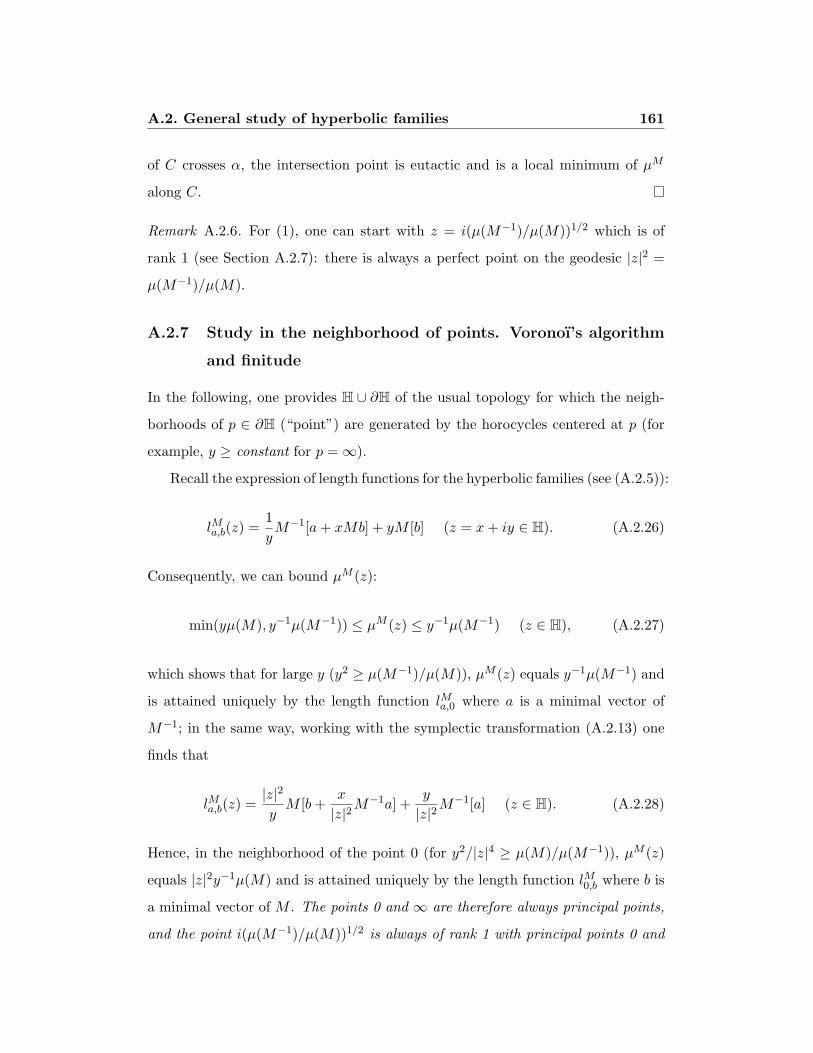
A.2. General study of hyperbolic families 161
of C crosses α, the intersection point is eutactic and is a local minimum of µM
along C.
Remark A.2.6. For (1), one can start with z = i(µ(M−1)/µ(M))1/2 which is of
rank 1 (see Section A.2.7): there is always a perfect point on the geodesic |z|2 =
µ(M−1)/µ(M).
A.2.7 Study in the neighborhood of points. Voronoı’s algorithm
and finitude
In the following, one provides H ∪ ∂H of the usual topology for which the neigh-
borhoods of p ∈ ∂H (“point”) are generated by the horocycles centered at p (for
example, y ≥ constant for p =∞).
Recall the expression of length functions for the hyperbolic families (see (A.2.5)):
lMa,b(z) =1yM−1[a+ xMb] + yM [b] (z = x+ iy ∈ H). (A.2.26)
Consequently, we can bound µM (z):
min(yµ(M), y−1µ(M−1)) ≤ µM (z) ≤ y−1µ(M−1) (z ∈ H), (A.2.27)
which shows that for large y (y2 ≥ µ(M−1)/µ(M)), µM (z) equals y−1µ(M−1) and
is attained uniquely by the length function lMa,0 where a is a minimal vector of
M−1; in the same way, working with the symplectic transformation (A.2.13) one
finds that
lMa,b(z) =|z|2
yM [b+
x
|z|2M−1a] +
y
|z|2M−1[a] (z ∈ H). (A.2.28)
Hence, in the neighborhood of the point 0 (for y2/|z|4 ≥ µ(M)/µ(M−1)), µM (z)
equals |z|2y−1µ(M) and is attained uniquely by the length function lM0,b where b is
a minimal vector of M . The points 0 and ∞ are therefore always principal points,
and the point i(µ(M−1)/µ(M))1/2 is always of rank 1 with principal points 0 and
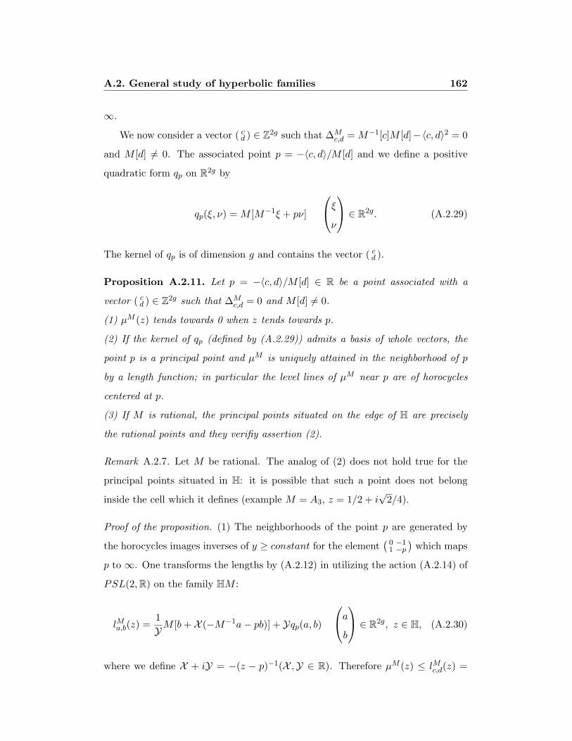
A.2. General study of hyperbolic families 162
∞.
We now consider a vector ( cd ) ∈ Z2g such that ∆M
c,d = M−1[c]M [d]−〈c, d〉2 = 0
and M [d] 6= 0. The associated point p = −〈c, d〉/M [d] and we define a positive
quadratic form qp on R2g by
qp(ξ, ν) = M [M−1ξ + pν]
ξν
∈ R2g. (A.2.29)
The kernel of qp is of dimension g and contains the vector ( cd ).
Proposition A.2.11. Let p = −〈c, d〉/M [d] ∈ R be a point associated with a
vector ( cd ) ∈ Z2g such that ∆M
c,d = 0 and M [d] 6= 0.
(1) µM (z) tends towards 0 when z tends towards p.
(2) If the kernel of qp (defined by (A.2.29)) admits a basis of whole vectors, the
point p is a principal point and µM is uniquely attained in the neighborhood of p
by a length function; in particular the level lines of µM near p are of horocycles
centered at p.
(3) If M is rational, the principal points situated on the edge of H are precisely
the rational points and they verifiy assertion (2).
Remark A.2.7. Let M be rational. The analog of (2) does not hold true for the
principal points situated in H: it is possible that such a point does not belong
inside the cell which it defines (example M = A3, z = 1/2 + i√
2/4).
Proof of the proposition. (1) The neighborhoods of the point p are generated by
the horocycles images inverses of y ≥ constant for the element(
0 −11 −p
)which maps
p to ∞. One transforms the lengths by (A.2.12) in utilizing the action (A.2.14) of
PSL(2,R) on the family HM :
lMa,b(z) =1YM [b+ X (−M−1a− pb)] + Yqp(a, b)
ab
∈ R2g, z ∈ H, (A.2.30)
where we define X + iY = −(z − p)−1(X ,Y ∈ R). Therefore µM (z) ≤ lMc,d(z) =

A.2. General study of hyperbolic families 163
M [d]/Y, which is assertion (1).
(2) The assumption on the kernel assures that qp admits on the whole vectors a
smaller nonzero value that we will denote µ1. Let µ2 be the minimum of M [b] for
whole nonzero vector ( ab ) in the kernel of qp (b 6= 0 because a = −pMb). Relation
(A.2.30) implies the inequalities
min(Yµ1,Y−1µ2) ≤ µM (z) ≤ Y−1µ2 (z ∈ H). (A.2.31)
From where it results that µM (z) = µ2/Y for Y2 ≥ µ2/µ1. The length functions
associated with the vectors ( ab ) of kernelN of qp are all proportional to lc,d (because
(M−1[a],M [b], 〈a, b〉) = M [b]M [d]−1(M−1[c],M [d], 〈c, d〉)), therefore for large Y,
µM (z) is uniquely attained by the length function la,b with ( ab ) ∈ N ∩ Z2g and
M [b] = µ2. An explicit example is given by Proposition A.3.2, Section A.3.3.
(3) If M is rational, the principal points are obviously rational. Let p ∈ Q be a
rational point distinct from ∞. Then there exist two whole vectors (c, d) 6= (0, 0)
such that M−1c + pd = 0, so that ∆Mc,d = 0 and p is associated with (c, d). The
assumption in assertion (2) on the kernel of qp is clearly satisfied: p is principal
and µM is attained in the neighborhood of p by a unique length function.
Corollary A.2.12. Let M be rational.
(1) Modulo the action of a subgroup Γ of finite index of PSL(2,Z), the tilings
DVM and DelM have only one finite number of regions of each dimension. In
particular the number of weakly eutactic points for µM is finite modulo Γ.
(2) There exists a “Voronoı” algorithm that can determine all of the perfect points
modulo Γ.
(3) Let C be a finite system of representatives modulo Γ of minimal classes of di-
mension 0, 1 and of two-dimensional minimal classes associated with the principal
points situated in H; let Γc be the stabilizer of c ∈ C. If χ indicates the Euler

A.2. General study of hyperbolic families 164
character, one has the relation
∑c∈C
(−1)dim c
card Γc= χ(Γ). (A.2.32)
(4) Let Pf be a finite system of representatives of perfect points modulo Γ. For
z ∈ Pf one notes that Az is the hyperbolic surface of the dual region of DelM of
z. With the notations of (3), one has the mass formula
∑z∈Pf
Az
card Γz= 2π |χ(Γ)| . (A.2.33)
Proof. One recalls that the family HM admits a complete symplectic action of a
subgroup of congruence Γ(m) (see Section A.2.2) and possibly of a subgroup Γ of
PSL(2,Z) containing Γ(m).
(1) From the proposition (assertions (2) and (3)) the skeleton of dimension 1 of
DVM , denoted (DVM )1, remain far from the rational points (which are finite in
number modulo Γ), i.e., in a compact part of Γ \H. The result follows.
(2) Assertion (1) and Theorem 1.1(4) show that the quotient Γ\(DVM )1 is a finite
and connected graph, of which the vertices are the perfect points for µM modulo
Γ. One can describe this graph thanks to Proposition A.2.10. One seeks initially a
perfect point and its neighbors, then the neighbors of new pefect points obtained
by the action of Π. At the end of a finite number of steps, one will have determined
all of the vertices of Γ \ (DVM )1. Note that one also obtains all of the eutactic
points modulo Γ (see Section A.2.5).
(3) Let us suppose initially that Γ acts without fixed points on H. Let ck (k =
0, 1, 2) be the number of k-dimensional regions of DVM modulo Γ (c0 is the number
of perfect points, and c2 is the number of principal points) and let cF2 be the number
of two-dimensional regions associated with the principal points situated in H. The
Euler-Poincare relation for the surface Γ\H supplemented by the points is written
c2 − c1 + c0 = 2− 2gΓ, (A.2.34)

A.2. General study of hyperbolic families 165
where gΓ is the genus of Γ. The character of Γ is given by χ(Γ) = cF2 − c1 + c0.
The general case (Γ with torsion) is easily obtained by passage to a subgroup
without torsion of finite index.
(4) The dual region of a perfect point z is a hyperbolic polygon generated by a
finite number of points of H ∪ δH (the principal points associated with z). Its
surface Az is therefore finite. As in (3), one begins by supposing that Γ is without
torsion, in which case one obviously has∑
z∈Pf Az = Surface(Γ \ H) = 2π|χ(Γ)|.
The general case results immediately. Note that the stabilizer of a perfect point
for the action of Γ coincides with that of its dual region.
Example. For Γ = Γ(m) (m ≤ 2) one has c2 − c1 + c0 = 2 − 2gm, where gm =
1 + km(m− 6)/(12m) with k2 = 6 and km = (m3/2)Πp|m(1− 1/p2) for m ≥ 3 (see
[Sh, p.22]).
Relations (A.2.32) and (A.2.33) (like (A.2.36)) are illustrated in Section A.3.5 with
M = An and Γ = Γ0(n+ 1) (1 ≤ n ≤ 16).
Remark A.2.8. (1) Let M be rational and z = x + iy be a perfect or eutactic
point for µM . Then x and |z|2 are rational (hence, y2 is rational). Indeed, the
principal points verify this property, and the geodesics which carry the edges of
the graph as those which join the principal points have an equation of the form
α|z|2 + βx + γ with α, β, γ ∈ Q. Consequently, the Gram matrix is proportional
to a whole matrix:
φg(zM) = λA A whole, λ2 ∈ Q, (A.2.35)
and, in particular, µ(zM)2 is rational.
(2) All that preceded also applies to matrices M which satisfy the hypotheses of
Proposition A.2.6: such a matrix is rational up to a factor as a single projective
solution of a homogeneous linear system with rational coefficients.
(3) If M = ( 1 ), (A.2.33) shows that the hexagonal lattice is the unique perfect
lattice in two dimensions. For the lattices of larger dimensions, we have a formula
analogous to (A.2.33), but we do not explicitly know the volumes.
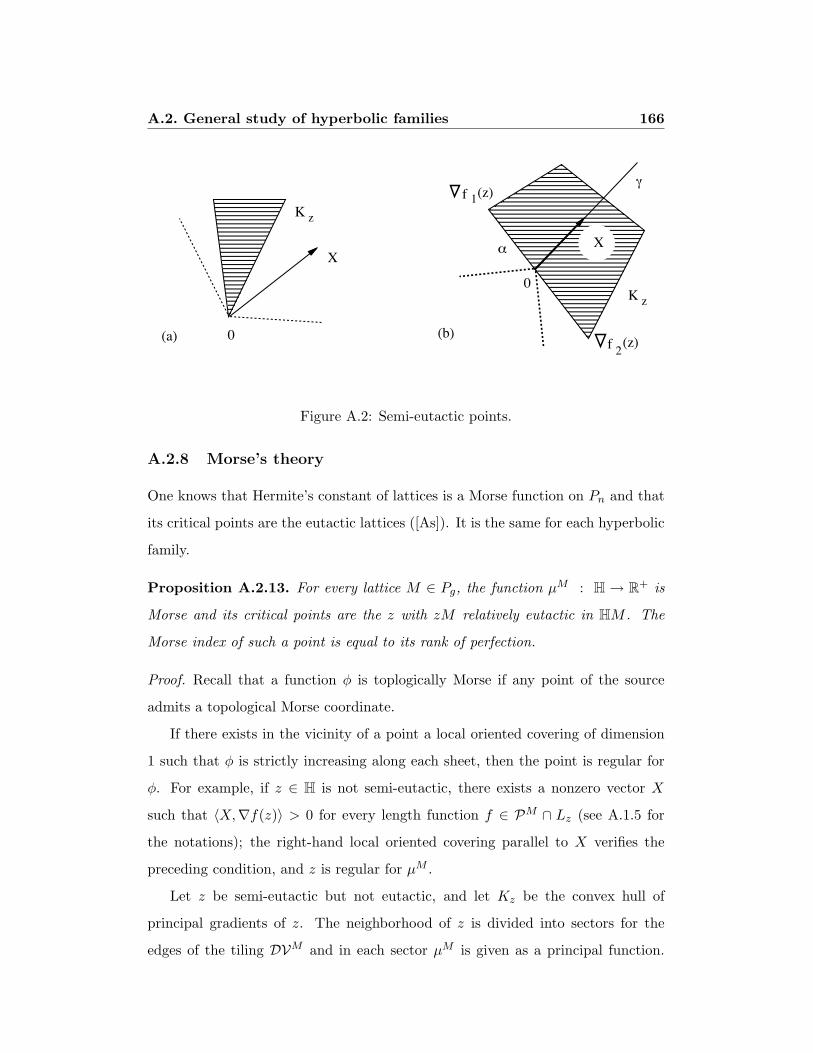
A.2. General study of hyperbolic families 166818 C. Bavard
(a)
X
0
K z
(b)
X
0
α
K z
1(z)f
2(z)f
γ
Fig. 2a,b. Points semi-eutactiques
strictement croissante le long de chaque feuille, alors le point est regulier pour ϕ.Par exemple, si z ∈ H n’est pas semi-eutactique, il existe un vecteur X non nultel que 〈X, ∇f (z)〉 > 0 pour toute fonction longueur f ∈ PM ∩ Lz (voir 1.5pour les notations); le feuilletage local oriente par droites paralleles a X verifiela condition precedente et z est regulier pour µM .Soit z semi-eutactique non eutactique et soit Kz l’enveloppe convexe des
gradients principaux en z. Le voisinage de z est divise en secteurs par les aretes dupavageDVM et dans chaque secteur µM est donnee par une fonction principale.Deux cas se presentent: 0 est un sommet de Kz ou 0 est a l’interieur d’une aretedeKz. Dans le premier cas z est un point principal, de la forme z = zf (f ∈ PM ).Il existe un vecteur X non nul tel que 〈X, Y 〉 > 0 pour tout Y ∈ Kz \ 0; Xest forcement a l’interieur du secteurΣf associe a f (Fig. 2a). Pour w voisin dez on pose X (w) = X. Si w ∈ Σf \ z, on a 〈X (w), ∇f (w)〉 > 0 car ∇f estradial a partir de z. La meme inegalite est vraie en tout point w pour les autresfonctions principales en z (par choix deX). D’ou il resulte queµM est strictementcroissante le long des orbites de X . Considerons maintenant le cas ou 0 est al’interieur d’une arete α deKz, enveloppe convexe de deux gradients principaux∇f (z) et ∇g(z). Notons Σf et Σg les secteurs fermes associes, separes par unedemi-geodesique γ (t) (t ≥ 0) de direction initiale X = γ ′(0) orthogonale a α(Fig. 2b). On definit alors un champ de vecteurs X continu par morceaux auvoisinage de z. Si w = γ (t) on prend X (w) = γ ′(t); si w ∈ Σf ∪ Σg \ γ il estpossible de choisir X (w) de classe C1 tel que limw→γ (t) X (w) = γ ′(t); enfinsi w /∈ Σf ∪ Σg on pose X (w) = X. Les orbites de X forment un feuilletageoriente C1 par morceaux et µM est strictement croissante le long des feuilles.Pour l’orbite de z cela resulte de la stricte convexite des fonctions longueur,et pour les autres de la condition 〈X (w), ∇h(w)〉 > 0 (h ∈ PM ∩ Lz). Onconclut que z est regulier. Remarquer que le niveau du point z admet un point derebroussement en z.Pour achever la preuve de la proposition, on observe que les points eutac-
tiques de rang k sont deMorse d’indice k (k = 0, 1, 2). Par exemple, au voisinaged’un point z eutactique de rang 1, µM est le minimum de deux fonctions stricte-
Figure A.2: Semi-eutactic points.
A.2.8 Morse’s theory
One knows that Hermite’s constant of lattices is a Morse function on Pn and that
its critical points are the eutactic lattices ([As]). It is the same for each hyperbolic
family.
Proposition A.2.13. For every lattice M ∈ Pg, the function µM : H → R+ is
Morse and its critical points are the z with zM relatively eutactic in HM . The
Morse index of such a point is equal to its rank of perfection.
Proof. Recall that a function φ is toplogically Morse if any point of the source
admits a topological Morse coordinate.
If there exists in the vicinity of a point a local oriented covering of dimension
1 such that φ is strictly increasing along each sheet, then the point is regular for
φ. For example, if z ∈ H is not semi-eutactic, there exists a nonzero vector X
such that 〈X,∇f(z)〉 > 0 for every length function f ∈ PM ∩ Lz (see A.1.5 for
the notations); the right-hand local oriented covering parallel to X verifies the
preceding condition, and z is regular for µM .
Let z be semi-eutactic but not eutactic, and let Kz be the convex hull of
principal gradients of z. The neighborhood of z is divided into sectors for the
edges of the tiling DVM and in each sector µM is given as a principal function.

A.2. General study of hyperbolic families 167
Two cases are presented: 0 is a vertex of Kz or 0 is in the interior of an edge of
Kz. In the first case z is a principal point of the lattice z = zf (f ∈ PM ). There
exists a nonzero vector X such that 〈X,Y 〉 > 0 for all Y ∈ Kz \0; X is inevitably
inside the sector∑
f associated with f (Figure A.2a). For w close to z, we define
X (w) = X. If w ∈∑
f \z, we have 〈X (w),∇f(w) > 0 because ∇f is radial
from z. The same inequality holds true for any point w for the other principal
functions in z (by choice of X). This implies that µM is strictly increasing along
the orbits of X . Now consider the case where 0 is in the interior of an edge α of
Kz, the convex hull of two principal gradients ∇f(z) and ∇g(z). We denote∑
f
and∑
g as the assoicated closed sectors, separated by a semi-geodesic γ(t) (t ≥ 0)
with initial direction X = γ′(0) orthogonal to α (Figure A.2b). We then define
a champ of vectors X continuous by pieces in the vicinity of z. If w = γ(t) we
take X (w) = γ′(t); if w ∈∑
f ∪∑
g \γ there exists a choice X (w) of class C1 such
that limw→γ(t)X (w) = γ′(t); finally, if w /∈∑
f ∪∑
g we define X (w) = X. The
orbits of X piecewise form an oriented covering C1 and µM is strictly increasing
along the sheets. This is true for the orbit of z results due to the strict convexity
of the length functions and for theothers due to the condition 〈X (w),∇h(w)〉 > 0
(h ∈ PM ∩ Lz). We conclude that z is regular. Note that the level of the point z
admits a cusp at z.
To achieve the proof of the proposition, one observes that the eutactic points
of rank k have Morse index k (k = 0, 1, 2). For example, in the neighborhood of a
eutactic point z of rank 1, µM is the minimum of two strictly convex functions and
the singular level is the intersection of two curves (circles or horocycles) tangent
to z.
Remark A.2.9. Hermite’s constant on Siegel’s space Hg is not a Morse function
([Bv]).
Corollary A.2.14. Suppose M is rational and µM is invariant for a subgroup
Γ of finite index in PSL(2,Z). Let EΓ be a system of representatives of eutactic
points modulo Γ; we will denote Γz as the stabilizer of z (z ∈ EΓ) and indz as its

A.3. Examples 168
Morse index. These data determine the Euler character of Γ:
∑z∈EΓ
(−1)indz
card Γz= χ(Γ). (A.2.36)
Proof. Even if it means to take a subgroup of finite index, one can suppose that
Γ acts without fixed points. From Proposition A.2.11 (3), µM induces a Morse
function on the compact surface Γ \ (H ∪ Q ∪ ∞). Let ek be the number of
eutactic points of rank k = 0, 1, 2 modulo Γ; e2 is the number of extremal points
modulo Γ. We have the following relation:
e2 − e1 + e0 + νΓ = 2− 2gΓ, (A.2.37)
where νΓ is the number of points of Γ and gΓ is its genus. This proves the formula
for the case without torsion and the general case easily follows.
Remark A.2.10. The two relations of Euler (A.2.32) and (A.2.36) are analogous
but not always identical, because the number of eutactic points can be strictly lesser
than the number of minimal classes (modulo Γ). For example, this is the case for
the family HA3 (see Section A.3).
A.3 Examples
A.3.1 Families An. Forms F2n
This is the principal example of this article. As usual, An is the matrix defined by
An(j, k) = 1 (resp. 2) if j 6= k (resp. j = k) for n ≥ 2 and one agrees to set A1 =
( 1 ). The lattice An verifies the hypotheses of Proposition A.2.6: all the eutactic
(resp. semi-eutactic) points relative to HAn are eutactic (resp. semi-eutactic) in
P2n, therefore also in Hn. One draws aside the value n = 1 which corresponds to

A.3. Examples 169
the well-known case of two-dimensional lattices. The most interesting point is
z1,n =1
2(n+ 1)
(n+ i
√n(n+ 2)
)(n ≥ 2), (A.3.1)
lying on the geodesic |z|2 = n/2(n+1) where the lengths associated with the points
0 and ∞ (i.e., l0(z) = 2 |z|2 /y and l∞(z) = n/(n+ 1)y) are equal (see A.1.7).
Theorem A.3.1. The lattice F2n = z1,nAn(n ≥ 2) is extremal symplectic in Hn.
It admits (n+ 1)(3n+ 2)/2 pairs of minimal vectors of norm 2√n/(n+ 2).
Proof. Here is initially a method for determining the length functions taking a
small value at one point. The techniques used in this method will also be necessary
for the other examples studied in this article. M, z = x+ iy and λ ∈ R are given,
to find all the pairs (a, b) such that lMa,b(z) ≤ λ where
lMa,b(z) =1y(M−1[a] + 2x〈a, b〉+ |z|2M [b]) (z ∈ H). (A.3.2)
One starts by bounding M [b] and M−1[a] with the relations (A.2.26) and (A.2.28).
Then, for further limiting the possibilities, one bounds 〈a, b〉 using the inequality:
〈a, b〉2 ≤M−1[a]M [b]. (A.3.3)
Note that the equality in (A.3.3) occurs if and only if (M−1[a])1/2b = ±M [b]1/2
M−1a (one writes 〈a, b〉 = 〈M−1/2a,M1/2b〉 where M1/2 is a square root of M).
The explicit knowledge of M then provides a finite number of pairs (a, b),including
the minimum (and the minimal vectors) of the lattice zM .
For F2n = z1,nAn and λ = 2(n/(n+2))1/2, one is quickly led to a = 0, or b = 0,
or (knowing that An[b] is even) An[b] = 2, 〈a, b〉 = −1 and A−1n [a] = n/(n + 1).
On all these pairs (a, b), F2n has the value λ, which is therefore the minimum.
Thus z1,n admits three principal points: ∞, 0 and pn = (1 + i[(n − 1)/(n +
1)]1/2)/2. The associated minimal vectors (a, b) are respectively, expressed in the
natural basis (ej)1≤j≤n of Zn, (ej , 0) and (∑ej , 0) (n + 1 vectors), (0, ej) and

A.3. Examples 170
(0, ej − ek) (j 6= k, n(n + 1)/2 vectors), (ej ,−ej), (∑ej ,−ej), (−ej , ej − ek) and
(ek, ej − ek) (j 6= k, n(n+ 1) vectors).
We remark in summary that z1,n lies in the interior of its Delaunay region (a
triangle with vertices ∞, 0, pn); therefore F2n is eutactic in HAn (Theorem 1.1
(3)). This also results in the relation ∇∞ + ∇0 + n∇pn = 0 among the three
relative gradients (A.2.21). Consequently, F2n is eutactic in Hn and even in P2n
(Proposition A.2.5). It remains to be verified that the gradients of minimal vectors
in Hn generate their tangent space Sn(C). From (A.2.5) and the quadratic equation
2(n+ 1)z2 − 2nz + n = 0 satisfied by z1,n, one easily finds that
i∇a,b(z1,nAn) = [aa′ +12(Anba
′ + ab′An)]
+z21,n[Anbb
′An +n+ 1n
(Anba′ + ab′An)]. (A.3.4)
The R-vector space Sn(C) can be decomposed as Sn(C) = Sn(R) ⊕ z21,nSn(R).
The gradients (A.3.4) of the vectors associated with the point 0 generate the
component of z21,n (because An is perfect in Pn) and the first components of the
other “minimal” gradients (A.3.4) generate Sn(R); therefore F2n is perfect in the
symplectic sense. As in [B-M1] (see also [Bv, Section 3.3]) one concludes that F2n
is extremal in Hn.
Remark A.3.1. We know that F4 ' D4. For n ≥ 3 the lattice F2n is not perfect in
P2n for lack of minimal vectors.
A.3.2 Families An (continued). Forms G2n
Let us pass now to the study of the neighbors of z1,n for n ≥ 3. For reasons of
symmetry, two neighbors are obvious (−z1,n and 1− z1,n); the third is given by
z2,n =1
2(n+ 1)
(n+ i
√(n2 − 4)/3
)(n ≥ 4, n 6= 5) (A.3.5)
with z2,3 = (3 + i√
7)/8 and z2,5 = (5 + i√
11)/12. For n 6= 4, z2,n has principal
points 0, 1/2 and pn (see Lemma A.3.1).

A.3. Examples 171
Theorem A.3.2. The lattice G2n = z2,nAn (n ≥ 3) is extremal in P2n. For n ≥ 6,
its minimum value is 4(n−1)/√
3(n2 − 4) and it admits 2n(n+1) (resp. 147) pairs
of minimal vectors if n 6= 7 (resp. if n = 7).
Remark A.3.2. For n = 3, 4 and 5 one will be able to consult Table A.2 (G6 ' JK ,
Jacobian of the Klein manifold, and G8 ' E8). These particular cases show the
existence of small exceptional values of A−1n (see Lemma A.3.1): for n = 4 there
are more minimal vectors and for n = 3 or 5 the principal function associated with
the point 1/2 is “non-generic” (see Proposition A.3.2).
Proof. Let us suppose that n ≥ 6; the cases of n = 3, 4 and 5 are treated
analagously. For (A.3.2) one has that l0,b(z2,n) ≥ λn = 4(n−1)(3n2−12)−1/2 with
equality for An[b] = 2 (function associated with the point 0) and la,0(z2,n) > λn.
We now consider a 6= 0 and b 6= 0 such that la,b(z2,n) ≤ λn. The method shown in
Section A.3.1 gives the following bounds:
An[b] ≤ 8, A−1n [a] ≤ 8(n− 1)2
3(n2 − 4)and − 4 ≤ 〈a, b〉 ≤ −1. (A.3.6)
Next one examines the four possible values of a, b, and for each case the values
of An[b], knowing that the small values of A−1n [a] are defined by Lemma A.3.1.
After a rather long discussion (which also uses la,b(z2,n) ≤ λn and the inequality
(A.3.3)), one is led to two possibilities for (〈a, b〉,M [b], A−1n [a]): (−1, 2, n/(n+ 1))
which correspond to the principal point pn (see Lemma A.3.1) and (-4, 8, 2) which
gives a new principal point 1/2. The number of minimal vectors associated with
this point 1/2, given explicitly by Lemma A.3.1, is n(n+ 1)/2 (although there are
35 for n = 7). For n = 8, there are exceptional vectors such that A−1n [a] = 2 but
the b determined by the equality in (A.3.3) are not complete.
It is still necessary to establish that G2n is extremal in P2n. Eutaxy is verified
in HAn (Proposition A.2.6) in the same manner as for z1,n (see Lemma A.3.1).
For perfection, one considers the subspace of S2n(R) generated by(
aa′ ab′
ba′ bb′
)(with
minimal vector ( ab )) and one shows that its orthogonal for Tr(XY ) is reduced to

A.3. Examples 172
the zero vector. Let X =(
U VV ′ W
)∈ S2n(R) (where U and W are symmetric) be
such that
U [a] + 2a′V b+W [b] = 0 (A.3.7)
for all minimal vectors ( ab ) of G2n. In solving the linear equations, one finds that
W = 0 with the vectors of the point 0, and U = V = 0 with the other vectors. Up
to demonstrating Lemma A.3.1, this completes the proof of the theorem.
Lemma A.3.1. (small values of A−1n ) Let n ≥ 2, a ∈ Zn let (a 6= 0), let (ej)1≤j≤n
be the canonical basis of Zn and let u =∑
1≤j≤n ej. If A−1n [a] ≤ 8/3 there are
three possibilities:
• A−1n [a] = n/(n+ 1) and a = ej or a = u (n ≥ 2),
• A−1n [a] = 2(n− 1)/(n+ 1) and a = ej + ek (j 6= k) or a = u− ej (n ≥ 3),
• A−1n [a] = 2 and a = ej − ek (j 6= k) or a = u+ ej (n ≥ 2),
with the following exceptions:
• a = (2, 0) or a = (2, 2), A−1n [a] = 8/3,
• a = ei1 + . . .+ eip with
5 ≤ n ≤ 26, p = 3 or n− 2 and A−1n [a] = 3(n− 2)/(n+ 1),
or 7 ≤ n ≤ 11, p = 4 or n− 3 and A−1n [a] = 4(n− 3)/(n+ 1),
or n = 9, p = 5 and A−1n [a] = 5/2.
Proof of the lemma. Let us define a =∑
1≤j≤n ajej and ‖a‖∞ = max1≤j≤n |aj |.
Recall the expression
A−1n [a] =
∑1≤j≤n
a2j −
∑1≤j≤n
aj
2
/(n+ 1). (A.3.8)
The values of the coordinates aj are restricted according to the inequality (A.3.3)
by successively taking b = ej , ej − ek, ej + ek + el (n ≥ 3) and ej + ek − el − em

A.3. Examples 173
(n ≥ 4):
|aj | ≤ 2, |aj − ak| ≤ 2, |aj + ak + al| ≤ 5 and |aj + ak − al − am| ≤ 3. (A.3.9)
From (A.3.8) and (A.3.9), one then discusses the possibilities of ‖a‖∞ = 1 or 2.
A.3.3 Families An (continued). Forms H2n(ϕ) (ϕ ∈ SL2(Z))
In this paragraph, we pursue the exploration of perfect points of HAn. To each
element ϕ =(
α βγ δ
)we associate the point zϕ of H defined by
zϕ =2αβ + αδ + 2γδ + βγ + i
√3
2 (β2 + βδ + δ2)(A.3.10)
When n is large compared to the coefficients of ϕ, the point zϕ is perfect and even
gives an extremal point of Hn (Theorem 2.3). Its Delaunay region is the hyperbolic
triangle formed by the points γ/δ, (α + γ)/(δ + β) and α/β (αδ − βγ = 1). In
particular the successive neighbors of z2,n associated with the point 0 are of the
form
z(m) =2m− 1 + i
√3
2 (m2 −m+ 1)(m ≥ 3), (A.3.11)
which are perfect points when n ≥ 2m; z(m) is associated with ϕ =(
1 m−10 1
)and
therefore with the region (0, 1/m, 1/(m − 1)). We define H2n(m) = z(m)An and
H2n(ϕ) = zϕAn. The principal length functions of zϕ are made explicit in the
following proposition:
Proposition A.3.2. (principal functions associated with the points)
Let n ≥ 8 and let α/β be a rational point with β 6= 0, α and β relatively prime.
If n is even (resp. odd) suppose that n+ 1 does not divide β (resp. 2β). Then the
principal length function f associated with the point α/β is given by
f(z) =1y
(2α2 − 4αβx+ 2β2|z|2
)(z ∈ H). (A.3.12)
This is realized by n(n+1)/2 pairs of vectors ( ab ) ∈ Z2n (a = αa0 with A−1
n [a0] = 2

A.3. Examples 174
and b = −βA−1n a0).
For 2 ≤ n ≤ 7, the corresponding result is valid provided that β /∈ 2Z (resp.
7Z, 8Z) if n = 5 (resp. 6, 7).
Proof. Recall that the minimal vectors ( ab ) ∈ Z2n near the point α/β are deter-
mined by the relations A−1n [a]An[b] = 〈a, b〉2,−〈a, b〉/An[b] = α/β with An[b] a
minimum for these properties (see A.1.7). Suppose that α 6= 0 (see Lemma A.3.1
for α = 0). One also has that b = −(β/α)A−1n a = −(β/α)(a − 〈a, u〉u/(n + 1))
with u =∑n
j=1 ej ((A.3.3) in the case of equality), and of course b must be whole.
In calculating 〈b, u〉 one sees that (β/α) (〈a, u〉/(n + 1)) is whole; therefore βa/α
is whole and α divides a. We define a = αa0 with a0 ∈ Zn and remark that
A−1n [a0] = 2 gives the values indicated in the statement. There remains the pos-
sibility of A−1n [a0] < 2. The corresponding vectors a0 are explicit for Lemma
A.3.1, and one notes that n+ 1 divides β (resp. 2β) if A−1n [a0] = n/(n+ 1) (resp.
2(n− 1)/(n+ 1)). There are three exceptional values of A−1n [a0] < 2 of the lattice
3(n− 2)/(n+ 1) for n = 5, 6 or 7 (Lemma A.3.1), and by writing that b is whole
one finds the conditions announced for β.
Theorem A.3.3. Let n ≥ 9 and let ϕ =(
α βγ δ
)∈ SL(2,Z) with nonnegative
α, β, γ, δ and with 0 ≤ γδ ≤
αβ ≤
12 . If n ≥ 2(β+ δ) then the lattice H2n(ϕ) = zϕAn
is extremal in Hn and has 3n(n+ 1)/2 pairs of minimal vectors with norm 4/√
3.
Remark A.3.3. For 6 ≤ n ≤ 8 the forms we’re concerned with, i.e., due to the
isomorphism of H12(3) ' K12, H14(3) and H16(3) are also extremal symplectic
extremal with minimum 4/√
3, but with more minimal vectors (see Table A.2).
Proof. The point zϕ is l’image of z(3) = 5+i√
314 for ψ =
(α−2γ γβ−2δ δ
)∈ SL(2,Z).
This transformation envoie the points 0, 1/3, 1/2 on γ/δ, (α + γ)/(δ + β), α/β.
Following (A.2.11), the lattice H2n(ϕ) is the image of z(3)An under the action in
P2n of the element
P =(
δIn (β−2δ)A−1n
γAn (α−2γ)In
)∈ Sp(2n,Q). (A.3.13)

A.3. Examples 175
It is elementary to verify that the minimal vectors of points 0, 1/3 and 1/2
are mapped by P ′−1 to the points γ/δ, (α+ γ)/(δ + β) and α/β; all these vectors
are made explicit by Proposition A.3.2 (for example, for α/β: a = α(ej − ek) and
b = −β(ej − ek) or a = α(ej + u) and b = −βej up to a sign). We also remark
that the principal length functions of these three points take the same value 4/√
3
at the point zϕ, independently of ϕ. With these observations made, we can prove
the theorem by verifying that the minimum of H2n(ϕ) equals 4/√
3 (with the good
number of minimal vectors) and that H2n(3) is extremal symplectic. Indeed, the
3n(n+1)/2 minimal vectors of H2n(3) (associated with the points 0, 1/3 and 1/2)
form an extremal symplectic configuration and are transformed, in a nonwhole
way (which does not matter), in an extremal symplectic configuration of minimal
vectors of H2n(ϕ).
To determine the minimum of H2n(ϕ), we start by placing the length functions
in a form which reveals in a symmetrical way the three points γ/δ, (α+γ)/(δ+β)
and α/β. Let X = δa+ γAnb and Y = βa+ αAnb. A small calculation allows us
to verify that
lAna,b (zϕ) =
1√3
(A−1
n [X] +A−1n [Y ] +A−1
n [X + Y ]). (A.3.14)
This formula also arises rather naturally starting with relation (A.2.12) for the
transformation of lengths knowing that zϕ = ψ(5+i√
314 ). One is therefore led to the
following inequality:
A−1n [X] +A−1
n [Y ] +A−1n [Z] ≤ 4 (A.3.15)
with X, Y and Z satisfying X + Y + Z = 0. One sees with Lemma A.3.1 that
there exist two possibilities (for n ≥ 9): either one of the vectors X, Y or Z is zero,
or two of these vectors are minimal for A−1n . Let us examine the first possibility,
with for example Z = −X − Y = 0, i.e., (β + δ)a + (γ + α)Anb = 0. Since
(β + δ) and (γ + α) are relatively prime, a is divisible by (γ + δ) and necessarily
a = (γ + α)X, b = −(β + δ)A−1n X. Following (A.3.15), one has A−1
n [X] ≤ 2. If

A.3. Examples 176
A−1n [X] = 2(n−1)/(n+1) (resp. n/(n+1)) then the vector 2(β+δ)u/(n+1) (resp.
(β+ δ)u/(n+1)) must be whole, which is impossible since n ≥ 2(β+ δ). The only
possible value possible is therefore A−1n [X] = 2 which gives the minimal vectors of
the point (α+ δ)/(β + γ), with equality in (A.3.15). The case X = 0 or Y = 0 is
treated analagously and leads to the minimal vectors of points γ/δ or α/β (with
equality in (A.3.15)). Suppose now that X and Y are minimal vectors of A−1n .
One has b = A−1n (δY − βX), where (β ± δ)u/(n + 1) is whole, which is absurd.
The other cases are eliminated by the same method and finally the minimum of
H2n(ϕ) is shown to be 4/√
3 for n ≥ 2(β + δ).
It remains to be established thatH2n(3) is extremal. Eutaxy in P2n results from
the relative eutaxy in HAn (Proposition A.2.6), which is clear either geometrically
via Theorem A.2.1 (3), or algebraically (the sum of the three relative gradients
(A.2.21) is zero for z(3)). For perfection, one proceeds as in Section A.3.1 by
decomposing the gradients (A.2.5) in Hn as Sn(R) ⊕ z(3)2Sn(R). The gradients
associated with the point 0 generate the component of z(3)2 (see Section A.3.1).
For those of the point 1/2, the other component equals aa′ since Anb = −2a. Let
T = (tjk) ∈ Sn(R) such that Tr (aa′T ) = T [a] = 0 for a = ej − ek (j < k) and
a = ej +∑ej . One easily checks that T = 0, and therefore the gradients of points
0 and 1/2 generate their tangent space Sn(C) at the point z(3). Since z(3)An is
already eutactic (thanks to the third point!) one concludes that it is also perfect,
which completes the proof of the theorem.
Remark A.3.4. The forms H2n(ϕ) are rather similar at first sight because their
ensembles of minimal vectors are interchangeable by rational symplectic transfor-
mations (see (A.3.13)). They therefore have the same minimum, the same rank
of usual or symplectic perfection and the same usual or symplectic “spectrum”
(values of the (symplectic) lattice on the pairs of minimal vectors). However, they
are not always isomorphic: for n ≤ 16, the H2n(ϕ) coming from distinct points
z(ϕ) modulo Γ0(n+ 1) are pairwise nonisomorphic (see the comments that follow
Table A.2).

A.3. Examples 177
A.3.4 Families An (continued). Forms J4m−2
The perfect points of the preceding paragraph have every Delaunay region gener-
ated by three regular points in the sense of Proposition A.3.2. We give here an
example with an “irregular” point: 1/m with n = 2m−1. The associated principal
function equals 2(m−1)(1/m−2x+m|z|2)/y; this is realized by n(n+1)/2 vectors
( ab ) ∈ Z2n such that A−1
n [a] = 2(n− 1)/(n+ 1) and b = −mA−1n a, entirely due to
the relation n+ 1 = 2m. We define
w(m) =2m− 3 + i
√3− 4/m
2(m− 1)2(m ≥ 4). (A.3.16)
Theorem A.3.4. Let m ≥ 4. The form J4m−2 = w(m)A2m−1 is extremal in
H2m−1 with minimum 4(m − 1)/√m(3m− 4) for 3m(2m − 1) pairs of minimal
vectors.
Proof. One proceeds as in the proof of Theorem 2.3. The point w(m) will have
two regular principal points (0 and 1/(m − 1)) and one irregular principal point
(1/m). The lengths are written in a form adapted to these points:
lAna,b (w(m)) =
1m√
3− 4/m(mA−1
n [a] +mA−1n [(m− 1)a+Anb]
+ (m− 2)A−1n [ma+Anb]). (A.3.17)
In setting X = a and Y = (m− 1)a+Anb one is led to the inequality
mA−1n [X] +mA−1
n [Y ] + (m− 2)A−1n [X + Y ] ≤ 4(m− 1) (A.3.18)
analogous to (A.3.15) and which allows one to determine the minimum of J4m−2
and its minimal vectors.
The point w(m) satisfies the equation m(m− 1)2z2−m(2m− 3)z+m− 1 = 0,
and eutaxy of J4m−2 results from (m − 1)∇0 + (m − 2)∇1m + (m − 1)∇
1m−1 = 0,
relation between the relative gradients (of the point w(m)) associated with the
three principal points of w(m). Finally for the perfection of J4m−2 in H2m−1,

A.3. Examples 178
one proceeds as in Section A.3.3 by decomposing the tangent space in the form
Sn(C) = Sn(R)⊕ w(m)2Sn(R).
A.3.5 Extremal points of families An for 1 ≤ n ≤ 16
Here are some numeric data and some commentary on the families HAn for small
values of n. Table A.1 gives the number of eutactic points of families HAn for
1 ≤ n ≤ 16. The subgroup Γ of PSL(2,Z) which acts by complete symplectic
transformations on the family is Γ = PSL(2,Z) for n = 1 and Γ = Γ0(n + 1) for
n ≥ 2 (see (A.2.14) and (A.2.15)). The notations of Table A.1 are as following:
ind is the index of Γ in PSL(2,Z), (g, ν) its signature (genus, number of points)
and χ(Γ) its Euler character; e′k (k = 0, 1, 2) designates the number (dependent
on the stabilizers) of eutactic points of Morse index k counted modulo Γ. The two
Euler relations (A.2.32) and (A.2.36) are identical for all these examples except
for n = 3; in this case the number of classes is given by c0 = 4, c1 = 6 and cF2 = 1
(with the notations of Section A.2.7).
We indicate now the local maxima of µAn for 1 ≤ n ≤ 16, which gives all
extremal symplectic forms in Hn. In order to have the supplementary list of these
maxima modulo Γ0(n+ 1) it is appropriate to add the symmetries σ(z) = −z; we
mention only the points with Re (z) > 0 since the forms associated with z and
σ(z) have the same symplectic nature (Section A.2.2).
In Table A.2 one gives successively: n, the dimension of the parameter spaces
P2n and Hn, the points in H with the convention z = x+ iy = [x, y2], the square of
Hermite’s constant µ of the lattice zAn and a value approaching µ, the number of
pairs of minimal vectors (vm), the rank of perfection in P2n (“rg.u”) and the rank
of perfection in Hn (“rg.s”). In the last column (“not.”) one recalls the notations
used in this article.
The ranks of perfection of a lattice A ∈ Sn are determined starting from the
ensemble S(A) of its minimal vectors. The usual rank is equal to one less than
the vector rank of the system ss′; s ∈ S(A). For the symplectic rank, one can

A.3. Examples 179
Table A.1: Number of eutactic points in HAn (1 ≤ n ≤ 16).
n ind (g, ν) χ(Γ) e′2 e′1 e′0
1 1 (0,1) -1/6 1/3 1/2 0
2 4 (0,2) -2/3 2 3 1/3
3 6 (0,3) -1 4 5 0
4 6 (0,2) -1 3 5 1
5 12 (0,4) -2 6 9 1
6 8 (0,2) -4/3 14/3 7 1
7 12 (0,4) -2 6 9 1
8 12 (0,4) -2 6 9 1
9 18 (0,4) -3 8 12 1
10 12 (1,2) -2 6 9 1
11 24 (0,6) -4 10 15 1
12 14 (0,2) -7/3 20/3 10 1
13 24 (1,4) -4 10 15 1
14 24 (1,4) -4 10 15 1
15 24 (0,6) -4 10 15 1
16 18 (1,2) -3 8 12 1

A.3. Examples 180
utilize the gradients in Sn and (following [Bv, Section 3.4]) it is the affine rank of
the system of matrices ss′ + JAss′AJ ; s ∈ S(A)
(A.3.19)
with J =(
0 I−I 0
); one can also write A = ϕn(τ) (τ ∈ Hn) and work with the
gradients (A.2.5) in Hn. From the point of view of doing calculations, the second
solution is more advantageous because the dimension of Hn is half of that of P2n.
All these calculations can be reduced to operations on the rational numbers
(see Remark A.2.8, Section A.2.7) and have been implemented with the PARI
system.
The embedding (A.2.3) permits explicit Gram matrices for the lattices in Table
A.2. One finds in particular rather simple matrices for D4, A(2)6 ' JK (Jacobian
of the Klein quartic) and E8 (compare with [B-S, Appendix 2]).
All of the lattices in this list, with the exception of 29+i√
16784 A5, are of the type
F2n, G2n, H2n(m) or J2n (see Sects. 2.1, 2.2, 2.3 and 2.4). We can classify without
difficulty the perfect points of HAn for the following small values of n by utilizing
Voronoı’s algorithm (Corollary A.2.12 (2)). Another proof consists of verifying by
aid of the formula (A.2.33) which are of the forms F , G, H or J . For example,
for 9 ≤ n ≤ 16 one finds (modulo the action of the symmetry σ) the forms F2n,
G2n, H2n(3) (9 ≤ n ≤ 16), H2n(4) (11 ≤ n ≤ 16), J2n (n = 9, 11, 13, 15), as well as
H22(5) (n = 11), H28(5), H28(6) (n = 14) and H30(7) (n = 15). All these lattices
are extremal symplectic and no two are isomorphic to one another. The H2n(m)
cited here are always distinguished by the number of vectors with norm ≤ 2µ and
sometimes by Smith’s constant (see Remark 2.4).
Remark A.3.5. The study of eutactic points of HA2 leads to two eutactic forms
(i/√
3)A2 and (1/2 + i/√
12)A2 which are equivalent by SL(4,Z), but are not
so symplectically, i.e., by Sp(4,Z), because they differ by the rank of perfection
symplectic (which are resp. 3 and 4). One has therefore a flat torus which carries
two structures of distinct principally polarized abelian varieties.
The cases n = 3 and n = 4 are illustrated in Figure A.3 which describes the

A.3. Examples 181
Table A.2: Extremal symplectic points in HAn (1 ≤ n ≤ 8)
2n P2n Hn z µ2 µ ' vm rg.u rg.s rem. not.
1 2 2 [1/2, 3/4] 4/3 1.1547 3 2 2 A2 F2
2 9 6 [1/3, 2/9] 2 1.4142 12 9 6 D4 F4
3 20 12 [3/8, 15/64] 36/15 1.5491 22 18 12 F6
[3/8, 7/64] 16/7 1.5118 21 20 12 JK G6
4 35 20 [2/5, 6/25] 8/3 1.6329 35 30 20 F8
[2/5, 1/25] 4 2.0000 120 35 20 E8 G8
5 54 30 [5/12, 35/144] 20/7 1.6903 51 45 30 F10
[5/12, 11/144] 36/11 1.8090 55 54 30 G10
[29/84, 167/842] 576/167 1.8571 40 39 30
6 77 42 [3/7, 12/49] 3 1.7320 70 63 42 F12
[3/7, 8/147] 25/6 2.0412 84 77 42 G12
[5/14, 3/196] 16/3 2.3094 378 77 42 K12 H12(3)
7 104 56 [7/16, 63/256] 28/9 1.7638 92 84 56 F14
[7/16, 15/256] 64/15 2.0655 147 104 56 G14
[5/14, 3/196] 16/3 2.3094 119 83 56 H14(3)
[5/18, 1/162] 9/2 2.1213 84 83 56 J14
8 135 72 [4/9, 20/81] 16/5 1.7888 117 108 72 F16
[4/9, 5/81] 196/45 2.0870 144 135 72 G16
[5/14, 3/196] 16/3 2.3094 192 107 72 H16(3)

A.3. Examples 182830 C. Bavard
−~
n = 4
p
E
F
0 1/2
4
8
8
p4
σ
)γ (
F
0 1/2
p
F
J
J6
K3
6
3
12
−~
−~σ
n = 3
4
Fig. 3. Les familles HA3 et HA4
[5/14, 3/196], z13 = [1/4, 1/48], z14 = [25/147, 4/3(49)2], z15 = [7/60, 17/7(60)2], z16 = [88/567, 761/5672]. On rappelle la convention [x, u] = x +i√
u. Parmi ces 16 formes, 12 sont parfaites dans P16 (dont 11 extremes) et 12sont extremes dans H8. La famille Hlh2718 presente de nombreux phenomenesinteressants: points parfaits dont la cellule de Delaunay est entierement contenuedansH (z1 avec 5 points principaux, ou z12), points parfaits semi-eutactiques (z5,z13) et meme points parfaits faiblement eutactiques (z6, z14). Noter qu’une formeparfaite de Hn definie par un point faiblement eutactique d’une famille HM nepeut etre que faiblement eutactique dans Hn.
2.7 Autres exemples
Apres An, la deuxieme suite classique de reseaux est Dn (n ≥ 4). Les famillesassociees sont un peu decevantes car le groupe qui agit estΓ0(2) ouΓ0(4) suivantla parite de n. On trouve une seule forme extreme 1+i
2 Dn isomorphe a D+2n qui
est deja extreme dans P2n. Pour n = 4 on trouve a nouveau E8.Voici pour terminer une liste d’exemples de reseaux symplectiques parfaits
(tab. 3).A partir de la dimension 10, nous donnons seulement quelques exempleschoisis pour leur forte densite; il en existe beaucoup d’autres (nous avons obtenu64 points parfaits dans H5 et 230 points parfaits dans H6).Rappelons que les formes F2n,G2n etH2n(m) sont definies a partir deAn par
(2.1), (2.5) et (2.11).On noteFG2n la forme eutactiquen(1+i)/(2n+2)An;FG4est isomorphe a la forme eutactique de la classe a9 de [B-M2]. Nous utilisonsegalement les reseaux des differences de Craig construits a partir de An # A(1)
n
(voir par exemple [Ma]): si (ej )0≤j≤n est la base canonique de Rn+1, on noteA(k)
n (1 ≤ k ≤ n) la matrice de Gram des n vecteurs ui = ∑0≤j≤k(−1)j (kj)
ei+j (1 ≤ i ≤ n) de Rn+1 (les indices sont a prendre modulo n + 1). Dans laderniere colonne “not.” nous identifions les formes de type F , G ou H et nous
Figure A.3: The families HA3 and HA4.
global geometric situation. Only half of the fundamental domain is represented
(the rest is defined by the symmetry σ). The identifications operated by Γ0(4)
and Γ0(5) are clear. For n = 3, the group Γ0(4) is of index 6 with three points
0, ∞ and 1/2. There are four principal points: 0, ∞, 1/2 and p3 = (2 + i√
2)/4,
and therefore four regions of maximal dimension of which one is bounded (that
of p3). Each region comes with a principal length function (Section A.2.5) and a
certain number of minimal vectors, namely 6, 4, 3 and 12 associated with 0, ∞,
1/2 and p3, respectively (see Figure A.3). In this example, all minimizing length
functions are principal. One obtains therefore the number of minimal vectors on
the edges (which are always geodesic arcs in P2n of isodual symplectic forms) and
at the vertices of DVM by adding the contributions of neighboring regions. For
example the forms of the edge F6JK have eighteen minimal vectors. The principal
points of F6 are (0, ∞, p3), and those of JK are (p3, 0, 1/2) (the same modulo
Γ0(4), for σ(F6) and σ(JK)). The point (1 + i)/2 is denoted JF because 1+i2 A3
is isomorphic to the Jacobian of the Fermat quartic. The relation (A.2.33) here
becomes 2(π − θ) + 2θ = 2π|χ(Γ0(4))| with cos θ = 1/3. Finally, one remarks that
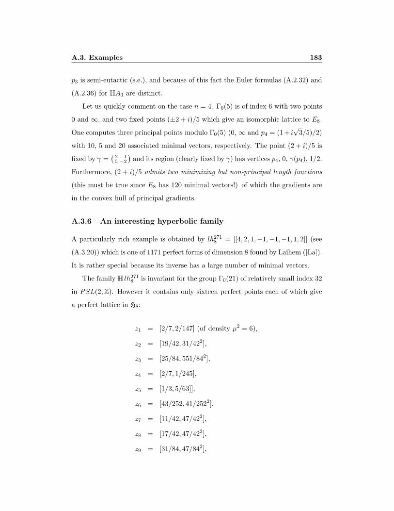
A.3. Examples 183
p3 is semi-eutactic (s.e.), and because of this fact the Euler formulas (A.2.32) and
(A.2.36) for HA3 are distinct.
Let us quickly comment on the case n = 4. Γ0(5) is of index 6 with two points
0 and ∞, and two fixed points (±2 + i)/5 which give an isomorphic lattice to E8.
One computes three principal points modulo Γ0(5) (0, ∞ and p4 = (1+ i√
3/5)/2)
with 10, 5 and 20 associated minimal vectors, respectively. The point (2 + i)/5 is
fixed by γ =(
2 −15 −2
)and its region (clearly fixed by γ) has vertices p4, 0, γ(p4), 1/2.
Furthermore, (2 + i)/5 admits two minimizing but non-principal length functions
(this must be true since E8 has 120 minimal vectors!) of which the gradients are
in the convex hull of principal gradients.
A.3.6 An interesting hyperbolic family
A particularly rich example is obtained by lh2718 = [[4, 2, 1,−1,−1,−1, 1, 2]] (see
(A.3.20)) which is one of 1171 perfect forms of dimension 8 found by Laıhem ([La]).
It is rather special because its inverse has a large number of minimal vectors.
The family H lh2718 is invariant for the group Γ0(21) of relatively small index 32
in PSL(2,Z). However it contains only sixteen perfect points each of which give
a perfect lattice in H8:
z1 = [2/7, 2/147] (of density µ2 = 6),
z2 = [19/42, 31/422],
z3 = [25/84, 551/842],
z4 = [2/7, 1/245],
z5 = [1/3, 5/63]],
z6 = [43/252, 41/2522],
z7 = [11/42, 47/422],
z8 = [17/42, 47/422],
z9 = [31/84, 47/842],

A.3. Examples 184
z10 = [25/84, 47/842]],
z11 = [3/7, 1/147],
z12 = [5/14, 3/196],
z13 = [1/4, 1/48],
z14 = [25/147, 4/3(49)2],
z15 = [7/60, 17/7(60)2],
z16 = [88/567, 761/5672].
One recalls the convention [x, u] = x + i√u. Among these sixteen forms, twelve
are perfect in P16 (of which eleven are extremal) and twelve are extremal in H8.
The family H lh2718 presents many interesting phenomena: perfect points of which
the Delaunay region is entirely contained in H (z1 with five principal points, or
z12), semi-eutactic perfect points (z5, z13) and even weakly eutactic perfect points
(z6, z14). Note that a perfect form of Hn defined for a weakly eutactic point of a
family HM can be only weakly eutactic in Hn.
A.3.7 Other examples
After An, the second classical set of lattices is Dn (n ≥ 4). The associated families
are a little disappointing because the group which acts is Γ0(2) or Γ0(4) according
to the parity of n. One finds only one extremal lattice 1+i2 Dn isomorphic to D+
2n
which is already extremal in P2n. For n = 4 one finds E8 again.
Here to finish is a list of examples of perfect symplectic lattices (Table A.3).
From dimension 10 and onwards, we give only some examples chosen for their good
density; there exist a large number of others (we have obtained 64 perfect points
in H5 and 230 perfect points in H6).
Recall that the forms F2n, G2n and H2n(m) are defined from An for (A.3.1),
(A.3.5) and (A.3.11). One notes that FG2n is the eutactic form n(1+i)/(2n+2)An;
FG4 is isomorphic to the eutactic form of the class a9 of [B-M2]. We also use
Craig’s difference lattices built starting from An ' A(1)n (see for example [Ma]):
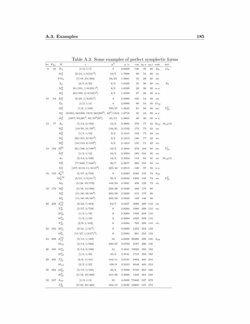
A.3. Examples 185
Table A.3: Some examples of perfect symplectic forms2n P2n M z µ2 µ ' vm rg.u rg.s rem. not.
8 35 D4 [1/2, 1/4] 4 2.0000 120 35 20 E8 G8
Ma4 [2/21, 1/5(21)2] 16/5 1.7888 60 34 20 ex.
FG4 [7/18, 23/324] 64/23 1.6681 33 28 20 ex.
A4 [2/5, 6/25] 8/3 1.6329 35 30 20 ex. F8
Mb4 [41/231, 1/6(231)2] 8/3 1.6329 29 26 20 w.e.
Mc4 [62/495, 2/3(165)2] 8/3 1.6329 27 26 20 w.e.
10 54 Ma5 [9/25, 1/4(25)2] 4 2.0000 130 54 30 ex.
D5 [1/2, 1/4] 4 2.0000 90 54 30 D10
Mb5 [1/6, 1/108] 100/27 1.9245 81 50 30 ex. T3
10
Mc5 [21991/481200, 1919/4812002] 822/1919 1.8718 45 44 30 w.e.
Md5 [1957/33(29)2, 65/332294] 45/13 1.8605 46 40 30 w.e.
12 77 A6 [5/14, 3/196] 16/3 2.3094 378 77 42 K12 H12(3)
Ma6 [19/56, 31/562] 144/31 2.1552 172 75 42 ex.
Mb6 [1/3, 1/18] 9/2 2.1213 192 75 42 ex.
Mc6 [60/451, 8/4512] 9/2 2.1213 180 77 42 ex.
Md6 [14/153, 8/1532] 9/2 2.1213 135 71 42 ex.
14 104 P307 [61/196, 3/1962] 16/3 2.3094 378 104 56 ex. T1
14
Ma7 [1/2, 1/12] 16/3 2.3094 189 104 56 ex.
A7 [5/14, 3/196] 16/3 2.3094 119 83 56 ex. H12(3)
Mb7 [77/848, 7/8482] 36/7 2.2677 280 104 56 ex.
Mc7 [157/4110, 11/41102] 225/44 2.2613 140 97 56 w.e.
16 135 A(2)8 [5/27, 2/729] 8 2.8284 2160 135 72 Λ16
lh1798 [5/21, 1/5(21)2] 36/5 2.6832 1200 135 72 ex. T2
16
M8 [5/24, 23/576] 144/23 2.5021 456 129 72 ex.
18 170 Ma9 [3/10, 13/300] 256/39 2.5620 480 170 90
Mb9 [11/40, 39/402] 256/39 2.5620 315 170 90
Mc9 [11/40, 39/402] 256/39 2.5620 189 146 90
20 209 A(2)10 [9/22, 7/484] 64/7 3.0237 3080 209 110 ex.
T310 [5/27, 2/729] 8 2.8284 1980 209 110 ex.
Ma10 [1/3, 1/18] 8 2.8284 1500 209 110
Mb10 [1/3, 1/18] 8 2.8284 1020 209 110
T310 [2/9, 1/162] 8 2.8284 765 209 110 ex.
22 252 Ma11 [9/41, 1/412] 9 3.0000 1232 252 132
Mb11 [11/27, 1/2(27)2] 8 2.8284 891 252 132
24 299 A(2)12 [5/13, 1/169] 16 4.0000 98280 299 156 Λ24
M12 [3/14, 1/588] 256/27 3.0792 2187 296 156
26 350 Ma13 [5/14, 3/196] 12 3.4641 10920 350 182
Mb13 [1/3, 1/45] 45/4 3.3541 1716 350 182
28 405 T114 [4/9, 11/81] 144/11 3.6181 9492 405 210
M14 [2/5, 1/25] 100/9 3.3333 6048 405 210
30 464 Ma15 [3/10, 1/100] 49/4 3.5000 6720 464 240
Mb15 [5/12, 19/288] 441/38 3.4066 1245 464 240
32 527 Λ16 [1/2, 1/4] 16 4.0000 73440 527 272
T216 [9/20, 39/400] 192/13 3.8430 22800 527 272

A.3. Examples 186
if (ej)0≤j≤n is the canonical basis for Rn+1, one notes that A(k)n (1 ≤ k ≤ n) is
the Gram matrix of n vectors ui =∑
0≤j≤k(−1)j(kj
)ei+j (1 ≤ i ≤ n) of Rn+1 (the
indices are to be taken modulo n + 1). In the last column “not.” we identify the
lattices of type F , G or H and we introduce some lattices T k2n useful for the higher
dimensions. The other basic used matrices are defined below.
For small dimensions, we specify in the column “rem.” the symplectic nature
of the forms (ex. = extremal, s.e. = semi-eutactic and w.e. = weakly eutactic).
The tests of eutaxy were carried out in MAPLE. For large dimensions, in order to
reduce the number of vectors to be considered, we replaced all the gradients which
have the same projection on HM with their sum, which allowed us to conclude
the eutaxy in certain cases. The calculation is even simpler when one can apply
Proposition A.2.6, such as for example, for A(k)p−1 with p prime (see in [Ma] p.138
the proof of Proposition 4.6).
To conclude, we mention the following question, suggested by the results of our
study.
Question. Let p be a prime number and let A(k)p−1(1 ≤ k ≤ p− 1) be the Craig
difference lattices. Up to p = 11, one notes that a relatively perfect point of the
family HA(k)p−1 is always perfect in Hp−1. Is this true for all p?
The list below (where we write “perf.” for perfect) supplements the data in
Table A.3, with the notation
[[a1, . . . , an]] = (a|i−j|+1)1≤i,j≤n. (A.3.20)
Ma4 = [[4, 2, 1, 1]],
M b4 = [[14, 11, 8, 8]],
M c4 = [[6, 1, 1, 1]],
Ma5 = [[4, 2, 1, 1, 2]],
M b5 = [[5, 2,−1,−1,−1]] (one of 136 eutactic quintic forms classified in [Bt]),
M c5 = [[10, 4, 1, 1, 4]],
Md5 = [[7, 1, 1, 1, 1]],

A.3. Examples 187
Ma6 = [[8, 3, 4, 6, 4, 3]],
M b6 = [[4, 1, 0, 1,−2,−2]],
M c6 = [[4, 0,−1, 0, 3, 1]],
Md6 = [[12, 1, 6,−2, 9, 1]],
P 307 = [[4, 1, 2, 2, 2, 2, 1]] (perf., see [Ja]),
Ma7 = [[3, 2, 1, 1, 1, 0, 0]],
M b7 = [[6, 3, 0,−1, 1, 1,−1]],
M c7 = [[9, 1, 1, 1, 1, 1, 1]],
lh1798 = [[6, 2,−2,−3,−1,−1, 0, 2]] (perf., see [The]),
M8 = [[6, 3, 1, 0,−3,−3,−2,−3]],
Ma9 = [[5, 3, 2, 2, 0, 0, 1, 0, 0]],
M b9 = [[4, 2, 1, 0, 1, 0, 0, 0, 1]] (perf.),
M c9 = [[4, 1, 0, 2, 2, 1, 0, 1, 2]],
Ma10 = [[4, 1, 0,−2,−1, 1, 1, 1,−1,−2]],
M b10 = [[4, 1,−1,−2, 0, 1, 2, 1,−2,−2]],
Ma11 = [[4, 1, 0, 0, 0, 0,−2,−1,−2,−2, 1]],
M b11 = [[4, 1, 0,−1,−2,−2, 0, 0, 0, 2, 2]] (perf.),
M12 = [[3, 1,−1,−1, 0, 1, 0,−1, 0, 1, 0,−1]],
Ma13 = [[3, 1,−1,−1, 0, 1, 0,−1, 0, 1, 0,−1,−1]],
M b13 = [[4,−2, 0, 1,−1, 1, 0, 0,−1, 1,−1, 0, 2]] (perf.),
M14 = [[4, 1,−1, 1, 1,−1, 0, 2, 1, 0, 0, 0, 0,−1]],
Ma15 = [[4, 2, 1, 0, 1, 1, 1, 1, 0,−1,−2,−1, 0, 0,−1]],
M b15 = [[4,−2, 2,−1, 0, 1,−1, 1,−2, 1,−2, 2,−2, 1,−1]].

A.3. Examples 188
References
[As] Ash A. On eutatic forms. Canad. J. Math. 29, 5 (1977), 1040–1054
[Bt] Batut C. Classification of quintic eutactic forms. Math. Comp. 70,
233 (2001), 395–417
[Bv] Bavard C. Systole et invariant d’Hermite. J. Reine Angew. Math.
482 (1997), 93–120
[B-M1] Berge A.-M., Martinet J. Densite dans de familles de reseaux. Ap-
plication aux reseaux isoduaux. Enseign. Math. 41 (1995), 335–
365
[B-M2] Berge A.-M., Martinet J. Sur la classification des reseaux eutac-
tiques. J. London Math. Soc. (2) 53 (1996), 417–432
[B-S] Buser P., Sarnak P. On the period matrix of a Riemann surface
of large genus (with an appendix by J. H. Conway and N. J. A.
Sloane). Invent. Math. 117 (1994), 27–56
[C-S] Conway J. H., Sloane N. J. A. Sphere packings, lattices and groups,
3rd ed. Springer-Verlag, NewYork, 1999
[Eb] Eberlein P. Structure of manifolds of nonpositive curvature. In
Global differential geometry and global analysis 1984 (Berlin,
1984). Springer, Berlin, 1985, 86–153. Springer L. N., Vol. 1156
[Ja] Jaquet-Chiffelle D. -O. Enumeration complete des classes de formes
parfaites en dimension 7. Ann. Inst. Forrier (Grenoble) 43, 1
(1993), 21–55
[La] Laıhem M. Construction algorithmique de reseaux parfaits. These,
Universite Bordeaux I, Dec. 1992
[Ma] Martinet J. Les reseaux parfaits des espaces euclidiens. Masson,
Paris, 1996
[Mu] Mumford D. Curves and their jacobians. The University of Michi-
gan Press, Ann Arbor, 1975
[Sc] Schmutz P. Riemann surfaces with shortest geodesic of maximal
length. Geom. Funct. Anal. 3, 6 (1993), 564–631
[Sh] Shimura G. Introduction to the arithmetic theory of automorphic
functions, vol. 11 of Publications of the Mathematical Society of
Japan. The Mathematical Society of Japan, 1971
189
Bibliography
[1] Dorit Aharonov and Michael Ben-Or. Fault-tolerant quantum computation
with constant error rate. 1999, quant-ph/9906129.
[2] Charlene Ahn and John Preskill. Cost of quantum fault-tolerance. In prepa-
ration, 2004.
[3] Miklos Ajtai. The shortest vector problem in L2 is NP-hard for randomized
reductions. Proceedings of the 30th Annual ACM Symposium on Theory of
Computing, pages 10–19, May 1998.
[4] Mark Alford, Kai-Ming Lee, John March-Russell, and John Preskill. Quantum
field theory of nonabelian strings and vortices. Nuclear Physics B, 384:251–
317, 1992, hep-th/9112038.
[5] Francisco Barahona. On the computational complexity of Ising spin-glass
models. Journal of Physics A, 15:3241–3253, 1982.
[6] Francisco Barahona, R. Maynard, R. Rammal, and J. P. Uhry. Morphology
of ground states of a two-dimensional frustration model. Journal of Physics
A, 15:673–699, 1982.
[7] Howard Barnum, Michael Nielsen, and Benjamin Schumacher. Information
transmission through a noisy quantum channel. Physical Review A, 57:4153–
4175, 1998, quant-ph/9702049.
[8] Christophe Bavard. Familles hyperboliques de reseaux symplectiques. Math-
ematische Annalen, 320(4):799–833, 2001.

190
[9] Dave Beckman, December 2000. Private communication.
[10] Charles Bennett and Giles Brassard. Quantum cryptography: Public key dis-
tribution and coin tossing. Proceedings of IEEE International Conference on
Computers Systems and Signal Processing, pages 175–179, December 1984,
www.research.ibm.com/people/b/bennetc/bennettc198469790513.pdf.
[11] Charles Bennett, David DiVincenzo, and John Smolin. Capacities of quan-
tum erasure channels. Physical Review Letters, 78:3217–3220, 1997, quant-
ph/9701015.
[12] Charles Bennett, David DiVincenzo, John Smolin, and William Wootters.
Mixed state entanglement and quantum error correction. Physical Review A,
54:3824–3851, 1996, quant-ph/9604024.
[13] Anne-Marie Berge. Symplectic lattices. Contemporary Mathematics, 272:9–22,
2000, www.math.u-bordeaux.fr/∼berge/symplectic.ps.
[14] Elwyn Berlekamp, John Conway, and Richard Guy. Winning Ways for Your
Mathematical Plays. Academic Press, London, 1982.
[15] Piotr Berman and Janos Simon. Investigations of fault-tolerant networks of
computers. Proceedings of the 20th Annual ACM Symposium on the Theory
of Computing, pages 66–77, 1988.
[16] Samuel Braunstein. Error correction for continuous quantum variables. Phys-
ical Review Letters, 80:4084–4087, 1998, quant-ph/9711049.
[17] Peter Buser and Peter Sarnak. On the period matrix of a Riemann surface of
large genus. Inventiones mathematicae, 117:27–56, 1994.
[18] Rob Calderbank, Eric Rains, Peter Shor, and Neil Sloane. Quantum error
correction and orthogonal geometry. Physical Review Letters, 78:405, 1997,
quant-ph/9605005.
191
[19] Rob Calderbank and Peter Shor. Good quantum error-correcting codes exist.
Physical Review A, 54:1098–1105, 1996, quant-ph/9512032.
[20] John W. S. Cassels. An introduction to the geometry of numbers. Springer-
Verlag, New York, 1971.
[21] John Conway and Neil Sloane. Sphere Packing, Lattices and Groups. Springer-
Verlag, New York, 3 edition, 1998.
[22] Thomas Cover and Joy Thomas. Elements of Information Theory. Wiley, New
York, 1991.
[23] Rudi de Buda. The upper error bound of a new near-optimal code. IEEE
Transactions in Information Theory, IT-21:441–445, 1975.
[24] Rudi de Buda. Some optimal codes have structure. IEEE Journal on Selected
Areas in Communications, 7(6):893–899, 1989.
[25] Philippe de Forcrand, Massimo D’Elia, and Michele Pepe. A study of the ’t
Hooft loop in SU(2) Yang-Mills theory. Physical Review Letters, 86:1438–1441,
2001, hep-lat/0007034.
[26] Eric Dennis, Alexei Kitaev, Andrew Landahl, and John Preskill. Topologi-
cal quantum memory. Journal of Mathematical Physics, 43:4452–4505, 2002,
quant-ph/0110143.
[27] David DiVincenzo, Peter Shor, and John Smolin. Quantum channel capac-
ity of very noisy channels. Physical Review A, 57:830–839, 1998, quant-
ph/9706061.
[28] Pierre Le Doussal and Brooks Harris. Location of the Ising spin-glass multi-
critical point on Nishimori’s line. Physical Review Letters, 61:625–628, 1988.
[29] Jack Edmonds. Paths, trees and flowers. Canadian Journal of Mathematics,
17:449–467, 1965.

192
[30] Richard Feynman. Simulating physics with computers. International Journal
of Theoretical Physics, 21:467–488, 1982.
[31] Peter Gacs. Reliable computation with cellular automata. Journal of Com-
puter and System Sciences, 32(1):15–78, 1986.
[32] Peter Gacs. Self-correcting two-dimensional arrays. Advances in Computing
Research, 5:223–326, 1989.
[33] Peter Gacs. Reliable cellular automata with self-organization. Journal of Sta-
tistical Physics, 103(1/2):45–267, 2001, math.PR/0003117.
[34] Peter Gacs and John Reif. A simple three-dimensional real-time reliable cel-
lular array. Journal of Computer and System Sciences, 36(2):125–147, April
1988.
[35] Daniel Gottesman. A class of quantum error-correcting codes saturating
the quantum Hamming bound. Physical Review A, 54:1862, 1996, quant-
ph/9604038.
[36] Daniel Gottesman. Stabilizer codes and quantum error correction. Caltech
Ph.D. Thesis, 1997, quant-ph/9705052.
[37] Daniel Gottesman. Fault-tolerant quantum computation with local gates.
Journal of Modern Optics, 47:333–345, 2000, quant-ph/9903099.
[38] Daniel Gottesman, Alexei Kitaev, and John Preskill. Encoding a qubit in an
oscillator. Physical Review A, 64:012310, 2001, quant-ph/0008040.
[39] Lawrence Gray. A reader’s guide to Gacs’s “Positive Rates” paper. Journal
of Statistical Physics, 103(1/2):1–44, 2001.
[40] Jim Harrington and John Preskill. Achievable rates for the Gaussian quantum
channel. Physical Review A, 64:062301, 2001, quant-ph/0105058.
[41] Alexander Holevo and Reinhard Werner. Evaluating capacities of bosonic
Gaussian channels. Physical Review A, 63:032312, 2001, quant-ph/9912067.

193
[42] Andreas Honecker, Marco Picco, and Pierre Pujol. Universality class of the
Nishimori point in the 2D ±J random-bond Ising model. Physical Review
Letters, 87:047201, 2001, cond-mat/00010143.
[43] Tsuyoshi Horiguchi and Tohru Morita. Existence of the ferromagnetic phase
in a random-bond Ising model on the square lattice. Journal of Physics A,
15:L75–L80, 1982.
[44] Naoki Kawashima and Heiko Rieger. Finite size scaling analysis of exact
ground states for±J spin glass models in two dimensions. Europhysics Letters,
39:85–90, 1997, cond-mat/9612116.
[45] Richard Kaye. Infinite versions of minesweeper are Turing complete. 2000,
http://web.mat.bham.ac.uk/R.W.Kaye/minesw/infmsw.pdf.
[46] Richard Kaye. Minesweeper is NP-complete. Mathematical Intelligencer,
22(2):9–15, 2000, web.mat.bham.ac.uk/R.W.Kaye/minesw/ordmsw.htm.
[47] Alexei Kitaev. Quantum error correction with imperfect gates. Proceedings of
the Third International Conference on Quantum Communication and Mea-
surement, 1997.
[48] Alexei Kitaev. Fault-tolerant quantum computation by anyons. Annals of
Physics, 303:2–30, 2003, quant-ph/9707021.
[49] Hidetsugu Kitatani. The verticality of the ferromagnetic-spin glass phase
boundary of the ±J Ising model in the p-t plane. Journal of the Physical
Society of Japan, 61:4049–4055, 1992.
[50] Greg Kuperberg, January 2004. Private communication.
[51] Hendrik Lenstra, Arjen Lenstra, and Laszlo Lovasz. Factoring polynomials
with rational coefficients. Mathematische Annalen, 261:515–534, 1982.
[52] Thomas Liggett. Interacting particle systems. Springer-Verlag, New York,
1985.

194
[53] Tamas Linder, Christian Schlegel, and Kenneth Zeger. Corrected proof of de
Buda’s theorem. IEEE Transactions in Information Theory, 39:1735–1737,
1993.
[54] Seth Lloyd. Universal quantum simulators. Science, 273:1073–1078, 1996.
[55] Seth Lloyd. The capacity of the noisy quantum channel. Physical Review A,
55:1613–1622, 1997, quant-ph/9604015.
[56] Seth Lloyd and Jean-Jacques Slotine. Analog quantum error correction. Phys-
ical Review Letters, 80:4088–4091, 1998, quant-ph/9711021.
[57] Genaro Martınez, Harold McIntosh, and Juan Mora. Production of gliders by
collisions in Rule 110. Advances in Artificial Life, 2801:175–182, 2003.
[58] Florian Merz and John Chalker. Two-dimensional random-bond Ising model,
free fermions, and the network model. Physical Review B, 65:054425, 2002,
cond-mat/0106023.
[59] Marc Mezard, Giorgio Parisi, and Miguel Virasoro. Spin Glass Theory and
Beyond. World Scientific, Singapore, 1987.
[60] Daniele Micciancio. The shortest vector in a lattice is hard to approximate to
within some constant. IEEE Symposium on Foundations of Computer Science,
pages 92–98, 1998, theory.lcs.mit.edu/∼miccianc/papers/svp.ps.
[61] Hermann Minkowski. Uber Geometrie der Zahlen. Gesammelte Abhandlungen,
1:264–265, 270, 277, 1911.
[62] Michael Nielsen and Isaac Chuang. Quantum Computation and Quantum In-
formation. Cambridge University Press, Cambridge, 2000.
[63] Hidetoshi Nishimori. Internal energy, specific heat, and correlation function of
the bond-random Ising model. Progress of Theoretical Physics, 66:1169–1181,
1981.

195
[64] Hidetoshi Nishimori. Geometry-induced phase transition in the ±J Ising
model. Journal of the Physical Society of Japan, 55:3305–3307, 1986.
[65] Hidetoshi Nishimori. Statistical Physics of Spin Glasses and Information Pro-
cessing. Oxford University Press, Oxford, 2001.
[66] Hidetoshi Nishimori. Derivatives and inequalities for order parameters in the
Ising spin glass. Journal of Phyiscs A: Mathematical and General, 35:9541–
9548, 2002, cond-mat/0206438.
[67] Hidetoshi Nishimori and Koji Nemoto. Duality and multicritical point of two-
dimensional spin glasses. Journal of the Physical Society of Japan, 71:1198–
1199, 2002, cond-mat/0111354.
[68] Fernando Nobre. Phase diagram of the two-dimensional ±J Ising spin glass.
Physical Review E, 64:046108, 2001.
[69] Harold Ollivier and Jean-Pierre Tillich. Description of a quantum convolu-
tional code. Physical Review Letters, 91:177902, 2003, quant-ph/0304189.
[70] Harold Ollivier and Jean-Pierre Tillich. Quantum convolutional codes: fun-
damentals. 2004, quant-ph/0401134.
[71] William Poundstone. The Recursive Universe : Cosmic Complexity and the
Limits of Scientific Knowledge. Contemporary Books, Chicago, 1985.
[72] John Preskill. Lecture Notes for Physics 229: Quantum Information and Com-
putation. 1998, www.theory.caltech.edu/people/preskill/ph229.
[73] Eric Rains, November 2000. Private communication.
[74] Benjamin Schumacher and Michael Nielsen. Quantum data processing and
error correction. Physical Review A, 54:2629–2635, 1996, quant-ph/9604022.
[75] Claude Shannon. A mathematical theory of communication. Bell System Tech-
nical Journal, 27:379–423, 623–656, 1948.

196
[76] Peter Shor. Scheme for reducing decoherence in quantum computer memory.
Physical Review A, 52:2493–2496, 1995.
[77] Peter Shor. Fault-tolerant quantum computation. Proceedings of the 37th An-
nual Symposium on Foundations of Computer Science, pages 56–65, 1996,
quant-ph/9605011.
[78] Peter Shor. Polynomial-time algorithms for prime factorization and dis-
crete logarithms on a quantum computer. SIAM Journal on Computing,
26(5):1484–1509, 1997, quant-ph/9508027.
[79] Peter Shor and John Preskill. Simple proof of security of the BB84 quantum
key distribution protocol. Physical Review Letters, 85:441–444, 2000, quant-
ph/0003004.
[80] Andrew Steane. Error-correcting codes in quantum theory. Physical Review
Letters, 77:793–797, 1996.
[81] Andrew Steane. Multiple particle interference and quantum error cor-
rection. Proceedings: Mathematical, Physical and Engineering Sciences,
452(1954):2551–2577, 1996, quant-ph/9601029.
[82] Andrei Toom. Stable and attractive trajectories in multicomponent systems.
Advances in Probability, 6:549–575, 1980.
[83] Rudiger Urbanke and Bixio Rimoldi. Lattice codes can achieve capacity on
the AWGN channel. IEEE Transactions in Information Theory, 44:273–278,
1998.
[84] Chenyang Wang, Jim Harrington, and John Preskill. Confinement-Higgs tran-
sition in a disordered gauge theory and the accuracy threshold for quantum
memory. Annals of Physics, 303:31–58, 2003, quant-ph/0207088.
[85] Peter Young. Spin Glasses and Random Fields. World Scientific, Singapore,
1997.

197
Index
accuracy threshold, vi,
1, 2, 61, 63, 64,
78, 84, 85, 88, 89,
107–110, 113, 114,
128, 133, 137–139
Aharonov, Dorit, 138
Bavard, Christophe, 2,
46, 48, 140
Ben-Or, Michael, 138
Buser, Peter, 21–23, 25,
37
coherent information,
10, 11, 15, 22,
31–33, 37
one-shot, 9–11, 26,
30, 33, 37, 38, 59,
60
Conway, John, 46, 110
Cook, Matthew, 110
Edmonds, Jack, 86, 90,
104
fault-tolerant, 2, 62, 78,
110, 135
Gacs, Peter, 109–112,
114, 116, 117, 138
Gaussian
classical channel, 11,
13, 23, 33, 35, 36
quantum channel, v,
1, 9–11, 14, 15, 20,
26, 27, 33, 37, 39,
40, 50, 51, 57, 58,
60
Gottesman, Daniel, 3,
138
Gram matrix, 50, 51,
53, 56
Gray, Larry, 112, 124,
127, 128
kissing number, 7, 53,
56
Kitaev, Alexei, 62, 109
Monte Carlo, 2, 58, 61,
105, 106, 135
Nishimori
line, 61, 62, 64, 65,
69–72, 76–78, 85,
86, 89, 106, 107
point, 69–72, 85, 89,
92, 98
relation, 63, 85, 88,
106
Nishimori, Hidetoshi,
64, 69, 70, 72, 77,
89, 98
Sarnak, Peter, 21–23,
25, 37
Sloane, Neil, 46
symplectic
inner product, 8, 16,
41, 44, 47
self-dual, v, 8, 18,
19, 21–23, 25, 26,
39, 40, 42, 44, 46,
47, 49, 50, 60
Voronoi cell, 8, 20,
23–25, 41, 51–54,
58