Embed Size (px)
Citation preview

1
1
Analysis Of Preventive Intervention DataUsing Mixture Modeling In Mplus
Bengt MuthénUCLA
Society for Prevention Research pre-conference workshop,Washington DC, May 29, 2007
2
• Inefficient dissemination of statistical methods:– Many good methods contributions from biostatistics,
psychometrics, etc are underutilized in practice• Fragmented presentation of methods:
– Technical descriptions in many different journals– Many different pieces of limited software
• Mplus: Integration of methods in one framework– Easy to use: Simple, non-technical language, graphics– Powerful: General modeling capabilities
Mplus Background
• Mplus versions– V1: November 1998– V3: March 2004
– V2: February 2001– V4: February 2006
• Mplus team: Linda & Bengt Muthén, Thuy Nguyen, Tihomir Asparouhov, Michelle Conn

2
3
Statistical Analysis With Latent VariablesA General Modeling Framework
Statistical Concepts Captured By Latent Variables
• Measurement errors• Factors• Random effects• Frailties, liabilities• Variance components• Missing data
• Latent classes• Clusters• Finite mixtures• Missing data
Continuous Latent Variables Categorical Latent Variables
4
Statistical Analysis With Latent VariablesA General Modeling Framework (Continued)
• Factor analysis models• Structural equation models• Growth curve models• Multilevel models
• Latent class models• Mixture models• Discrete-time survival models• Missing data models
Models That Use Latent Variables
Mplus integrates the statistical concepts captured by latent variables into a general modeling framework that includes not only all of the models listed above but also combinations and extensions of these models.
Continuous Latent Variables Categorical Latent Variables
3
5
General Latent Variable Modeling Framework
• Observed variablesx background variables (no model structure)y continuous and censored outcome variablesu categorical (dichotomous, ordinal, nominal) and
count outcome variables• Latent variables
f continuous variables– interactions among f’s
c categorical variables– multiple c’s
6
Mplus
Several programs in one
• Structural equation modeling
• Item response theory analysis
• Latent class analysis
• Latent transition analysis
• Survival analysis
• Multilevel analysis
• Complex survey data analysis
• Monte Carlo simulation
Fully integrated in the general latent variable framework

4
7
OverviewSingle-Level Analysis
Day 4Latent Transition Analysis
Latent Class Growth AnalysisGrowth Analysis
Growth Mixture Modeling Discrete-Time Survival
Mixture Analysis Missing Data Analysis
Day 3Regression Analysis
Path AnalysisExploratory Factor Analysis
Confirmatory Factor Analysis Structural Equation Modeling
Latent Class Analysis Factor Mixture Analysis
Structural Equation Mixture Modeling
Adding Categorical Observed And LatentVariables
Day 2Growth Analysis
Day 1Regression Analysis
Path AnalysisExploratory Factor Analysis
Confirmatory Factor Analysis Structural Equation Modeling
Continuous Observed And Latent Variables
LongitudinalCross-Sectional
8
Day 5Growth Mixture Modeling
Day 5Latent Class Analysis
Factor Mixture Analysis
Adding Categorical Observed And LatentVariables
Day 5Growth Analysis
Day 5Regression Analysis
Path AnalysisExploratory Factor Analysis
Confirmatory Factor Analysis Structural Equation Modeling
Continuous Observed And Latent Variables
LongitudinalCross-Sectional
Overview (Continued)
Multilevel Analysis

5
9
Further Studies• Mplus web site: www.statmodel.com
• Short courses
• Johns Hopkins University, August 20-22, 2007 (twice a year): Multilevel modeling
• University of Florence, Italy, September 10-12, 2007: Mixture, growth, and multilevel modeling
• Web videos of courses: 10 weeks, 2 days, 1 day, 2 hours
• Reference section
• Paper section (pdf’s)
• Free demo and Mplus User's Guide
• Mplus Discussion
• Syllabus, handouts and suggested readings from the UCLA course Statistical Methods for School-Based Intervention Studies, http://www.gseis.ucla.edu/faculty/muthen/courses_Ed255C.htm
10
Data For Longitudinal Intervention Studies
• Baseline individual measures (covariates, measurement instruments)
• Influencing control group development
• Influencing treatment group development
• Influencing dropout
• Baseline outcomes
time
During intervention
After intervention
• Outcomes• Proximal• Distal
Before intervention
• Implementation measures
• Compliance measures

6
11
Finding Subgroups By Mixture Modeling• Baseline data analysis: Latent class analysis
• Analysis of developmental trajectory classes in the absence of intervention– Latent transition analysis– Growth mixture analysis
• Analysis of developmental trajectory classes in the presence of intervention - for whom is an intervention effective?
12
Latent Class Analysis

7
13
c
x
inatt1 inatt2 hyper1 hyper21.0
0.9
0.80.70.60.50.40.30.20.1
Latent Class Analysis
inat
t1Class 2
Class 3
Class 4
Class 1
Item Probability
Item
inat
t2
hype
r1
hype
r2
14
Latent Class Analysis (Continued)Introduced by Lazarsfeld & Henry, Goodman, Clogg, Dayton & Mcready
• Setting– Cross-sectional data– Multiple items measuring a construct– Hypothesized construct represented as latent class variable (categorical
latent variable
• Aim– Identify items that indicate classes well– Estimate class probabilities– Relate class probabilities to covariates– Classify individuals into classes (posterior probabilities)
• Applications– Diagnostic criteria for alcohol dependence. National sample, n = 8313– Antisocial behavior items measured in the NLSY. National sample,
n = 7326

8
15
Latent Class Analysis ModelDichotomous (0/1) indicators u: u1, u2, … , ur
Categorical latent variable c: c = k ; k = 1, 2, … , K.
Marginal probability for item uj = 1,
Joint probability of all u’s, assuming conditional independence
P(u1, u2, … , ur) =
P(c = k) P(u1 | c = k) P(u2 | c = k) … P(ur | c = k)
Note analogies with the case of continuous outcomes and continuousfactors
ΣK
k = 1
ΣK
k = 1
u1 u2 u3
c
P(uj = 1) = P(c = k) P(uj = 1 | c = k).
16
LCA Estimation
Posterior Probabilities:
P(c = k | u1, u2, … , ur) =
Maximum-likelihood estimation via the EM algorithm:c seen as missing data. EM: maximize E(complete-data log likelihood |ui1, ui2 ,…, uir) wrt parameters.
• E (Expectation) step: compute E(ci | ui1,ui2,…,uir) = posterior probability for each class and E(ci uij | ui1, ui2,…,uir) for each class and uj
• M (Maximization) step: estimate P(uj | ck) and P(ck) parameters by regression and summation over posterior probabilities
P(c = k) P(u1 | c = k) P(u2 | c = k)…P(ur | c = k)P(u1, u2, … , ur)

9
17
Number of H0 parameters in the (exploratory) LCA model with Kclasses and r binary u’s: K – 1 + K × r (H1 has 2r – 1 parameters).
H1 H0• 2 classes, 3 u: df = 0 computed as (8 – 1) – (1 + 6)• 2 classes, 4 u: df = 6 computed as (16 – 1) – (1 + 8)• 3 classes, 4 u: df = 1, but not identified because of 1 indeterminacy• 3 classes, 5 u: df = 14 computed as (32 – 1) – (2 + 15)
Confirmatory LCA modeling applies restrictions to the parameters.
Logit versus Probability Scale. The u-c relation is a logit regression (binary u),
P(u = 1 | c) = , (81)
Logit = log [P/(1 – P)]. (82) For example:Logit = 0: P = 0.5Logit = -1: P = 0.27Logit = 1: P = 0.73
LCA Parameters
11 + exp (–Logit)
Logit = -3: P = 0.05Logit = -10: P = 0.00005
18
• Model fit to frequency tables. Overall test against data– When the model contains only u, summing over the cells,
χP = , (82)
χLR = 2 oi log oi / ei . (83)
LCA Testing Against Data
A cell that has non-zero observed frequency and expectedfrequency less than .01 is not included in the χ2 computation asthe default. With missing data on u, the EM algorithmdescribed in Little and Rubin (1987; chapter 9.3, pp. 181-185)is used to compute the estimated frequencies in the unrestrictedmultinomial model. In this case, a test of MCAR for theunrestricted model is also provided (Little & Rubin, 1987, pp.192-193).
• Model fit to univariate and bivariate frequency tables. MplusTECH10
Σi
2 (oi – ei)2
ei
Σi
2

10
19
Latent Class AnalysisAlcohol Dependence Criteria, NLSY 1989 (n = 8313)
0.830.110.020.240.00Continue0.400.020.000.080.00Relief0.430.030.000.100.00Give up0.960.730.020.830.03Major role-Hazard0.650.090.000.190.00Time spent0.600.050.010.140.00Cut down0.990.940.120.960.15Larger0.810.350.010.450.01Tolerance0.490.070.000.140.00Withdrawal
DSM-III-R Criterion Conditional Probability of Fulfilling a Criterion0.030.210.750.220.78IIIIIIIII
Two-class solution1 Three-class solution2
1Likelihood ratio chi-square fit = 1779 with 492 degrees of freedom2Likelihood ratio chi-square fit = 448 with 482 degrees of freedom
Prevalence
Latent Classes
Source: Muthén & Muthén (1995)
20
Latent Class Membership By Number Of DSM-III-RAlcohol Dependence Criteria Met (n=8313)
24002400.39
18.6
0001921146984510
3.378.121.978.1100.0%
3903900.584204200.576806800.8697011601.452021302.640046905.6300845010.22011611116114.01053350533564.20
IIIIIIIII
Two-class solution Three-class solutionNumber ofCriteria Met
%
Latent ClassesSource: Muthén & Muthén (1995)

11
21
LCA Testing Of K – 1 Versus K Classes
Model testing by χ2, BIC, and LRT
• Overall test against data: likelihood-ratio χ2 with H1 as the unrestricted multinomial (problem: sparse cells)
• Comparing models with different number of classes:− Likelihood-ratio χ2 cannot be used– Bayesian information criterion (Schwartz, 1978)
BIC = –2logL + h × ln n, (81)where h is the number of parameters and n is the sample size.Choose model with smallest BIC value.
– Vuong-Lo-Mendell-Rubin likelihood-ratio test (Biometrika, 2001). Mplus TECH11
– Bootstrapped likelihood ratio test. Mplus TECH14 (Version 4)
22
Other Considerations In DeterminingThe Number Of Classes
Interpretability and usefulness:• Substantive theory• Auxiliary (external) variables• Predictive validity

12
23
01484# significant bivariateresiduals (TECH10)
0.0000.0000.0000.000BLRT (TECH14) p0.8520.8440.8920.901Entropy
0.0820.0080.0000.000LMR (TECH11) p28,53528,50828,53929,780BIC
49392919# of parameters-14,046-14,078-14,139-14,804Loglikelihood
462472482492χ2 df2633264481,779LR χ2
585664773128,906Pearson χ2
5432Number of Classes
LCA Model Results For NLSY Alcohol Dependence Criteria
24
With
draw
al
Tole
ranc
e
Larg
er
Cut
dow
n
Tim
e sp
ent
Maj
or ro
le -
Haz
ard
Giv
e up
Rel
ief
Con
tinue
Item
0
0.05
0.1
0.15
0.2
0.25
0.3
0.35
0.4
0.45
0.5
0.55
0.6
0.65
0.7
0.75
0.8
0.85
0.9
0.95
1
Pro
babi
lity
Class 1, 21.6%
Class 2, 78.4%
With
draw
al
Tole
ranc
e
Larg
er
Cut
dow
n
Tim
e sp
ent
Maj
or ro
le-H
azar
d
Giv
e up
Rel
ief
Con
tinue
Item
0
0.05
0.1
0.15
0.2
0.25
0.3
0.35
0.4
0.45
0.5
0.55
0.6
0.65
0.7
0.75
0.8
0.85
0.9
0.95
1
Pro
babi
lity
Class 1, 18.4%
Class 2, 1.8%
Class 3, 72.5%
Class 4, 1.6%
Class 5, 5.7%
2-class LCA Item Profiles
LCA Item Profiles For NLSY Alcohol Criteria
With
draw
al
Tole
ranc
e
Larg
er
Cut
dow
n
Tim
e sp
ent
Maj
or ro
le-H
azar
d
Giv
e up
Rel
ief
Con
tinue
Item
0
0.05
0.1
0.15
0.2
0.25
0.3
0.35
0.4
0.45
0.5
0.55
0.6
0.65
0.7
0.75
0.8
0.85
0.9
0.95
1
Pro
babi
lity
Class 1, 75.4%
Class 2, 3.4%
Class 3, 21.2%
3-class LCA Item Profiles
4-class LCA Item Profiles 5-class LCA Item Profiles
With
draw
al
Tole
ranc
e
Larg
er
Cut
dow
n
Tim
e sp
ent
Maj
or ro
le-H
azar
d
Giv
e up
Rel
ief
Con
tinue
Item
0
0.05
0.1
0.15
0.2
0.25
0.3
0.35
0.4
0.45
0.5
0.55
0.6
0.65
0.7
0.75
0.8
0.85
0.9
0.95
1
Pro
babi
lity
Class 1, 1.5%
Class 2, 72.2%
Class 3, 19.5%
Class 4, 6.8%
13
25
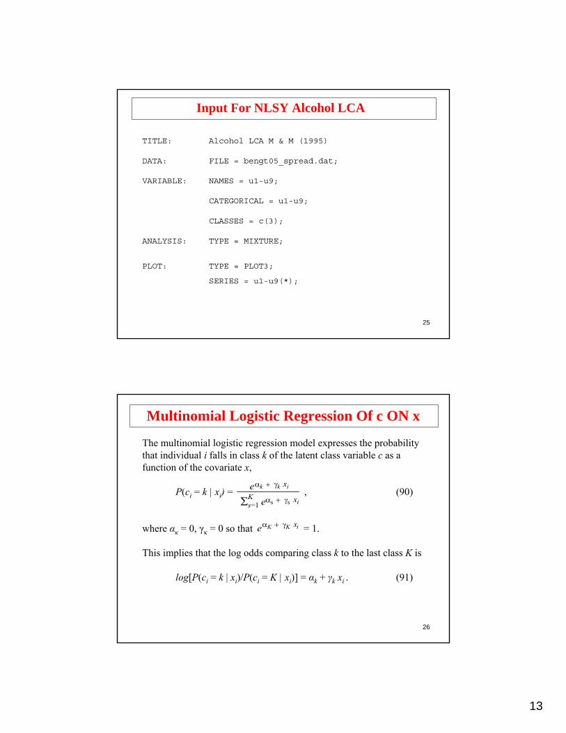
Input For NLSY Alcohol LCA
TITLE: Alcohol LCA M & M (1995)
DATA: FILE = bengt05_spread.dat;
VARIABLE: NAMES = u1-u9;
CATEGORICAL = u1-u9;
CLASSES = c(3);
ANALYSIS: TYPE = MIXTURE;
PLOT: TYPE = PLOT3;
SERIES = u1-u9(*);
26
The multinomial logistic regression model expresses the probabilitythat individual i falls in class k of the latent class variable c as afunction of the covariate x,
P(ci = k | xi) = , (90)
where ακ = 0, γκ = 0 so that = 1.
This implies that the log odds comparing class k to the last class K is
log[P(ci = k | xi)/P(ci = K | xi)] = αk + γk xi . (91)
Multinomial Logistic Regression Of c ON x
ΣKs=1 eαs + γs xi
αk + γk xie
αK + γK xie

14
27
White Males White Females
Black Males Black Females
CLASS 1CLASS 2
CLASS 3CLASS 4
CLASS 1CLASS 2
CLASS 3CLASS 4
CLASS 1CLASS 2
CLASS 3CLASS 4
CLASS 1CLASS 2
CLASS 3CLASS 4
Pro
b
0.016 17 18 19 20 21 22 23AGE
Pro
b
16 17 18 19 20 21 22 23AGE
Pro
b
16 17 18 19 20 21 22 23AGE
Pro
b
16 17 18 19 20 21 22 23AGE
16
0.1
0.2
0.3
0.4
0.5
0.6
0.7
0.80.9
1.0
0.00.1
0.2
0.3
0.4
0.5
0.6
0.7
0.80.9
1.0
0.00.1
0.2
0.3
0.4
0.5
0.6
0.7
0.80.9
1.0
0.00.1
0.2
0.3
0.4
0.5
0.6
0.7
0.80.9
1.0
ASB Classes Regressed On Age,Male, Black In The NLSY (n=7326)
28
Clogg, C.C. (1995). Latent class models. In G. Arminger, C.C. Clogg& M.E. Sobel (eds.), Handbook of statistical modeling for the social and behavioral sciences (pp. 311-359). New York: Plenum Press.
Goodman, L.A. (1974). Exploratory latent structure analysis using both identifiable and unidentifiable models. Biometrika, 61, 215-231.
Hagenaars, J.A & McCutcheon, A. (2002). Applied latent class analysis. Cambridge: Cambridge University Press.
Nestadt, G., Hanfelt, J., Liang, K.Y., Lamacz, M., Wolyniec, P., & Pulver, A.E. (1994). An evaluation of the structure of schizophrenia spectrum personality disorders. Journal of Personality Disorders, 8, 288-298.
Rindskopf, D., & Rindskopf, W. (1986). The value of latent class analysis in medical diagnosis. Statistics in Medicine, 5, 21-27.
Uebersax, J.S., & Grove, W.M. (1990). Latent class analysis of diagnostic agreement. Statistics in Medicine, 9, 559-572.
Further Readings OnLatent Class Analysis

15
29
item 1 item 2 item 3 item 4
c
item 1 item 2 item 3 item 4
f
item 1 item 2 item 3 item 4
fc
Item j
Item k
Item kItem j
Item k
Item j1.0
0.5
0.1ite
m1
item
2
item
3
item
4
Class 2
Class 1
Item Probability
Item
1.0
0.5
0.1
item
1
item
2
item
3
item
4
Class 2
Class 1
Item Probability
Item
Latent Class Analysis
Factor Analysis (IRT)
Factor Mixture AnalysisFactor (f)
Item 1 Item 2Item 3Item 4
1.00.90.80.70.60.50.40.30.20.1
Item Probability
30
Latent Class, Factor, And Factor Mixture AnalysisAlcohol Dependence Criteria, NLSY 1989 (n = 8313)
0.830.110.020.240.00Continue0.400.020.000.080.00Relief0.430.030.000.100.00Give up0.960.730.020.830.03Major role-Hazard0.650.090.000.190.00Time spent0.600.050.010.140.00Cut down0.990.940.120.960.15Larger0.810.350.010.450.01Tolerance0.490.070.000.140.00Withdrawal
DSM-III-R Criterion Conditional Probability of Fulfilling a Criterion
0.030.210.750.220.78IIIIIIIII
Two-class solution1 Three-class solution2
1Likelihood ratio chi-square fit = 1779 with 492 degrees of freedom2Likelihood ratio chi-square fit = 448 with 482 degrees of freedom
Prevalence
Latent Classes
Source: Muthén & Muthén (1995)

16
31
LCA, FA, And FMA For NLSY 1989
• LCA, 3 classes: logL = -14,139, 29 parameters, BIC = 28,539• FA, 2 factors: logL = -14,083, 26 parameters, BIC = 28,401• FMA 2 classes, 1 factor, loadings invariant:
logL = -14,054, 29 parameters, BIC = 28,370
Models can be compared with respect to fit to the data
• Standardized bivariate residuals• Standardized residuals for most frequent response patterns
32
Estimated Frequencies And Standardized Residuals
Bolded entries are significant at the 5% level.
0.3345-0.3745-1.0940470110010010.3246-0.61440.8154480010110001.27593.80840.4252490100000001.6053-2.79460.4168650010010010.171471.451680.151511490000010001.87134-3.48118-4.161111550110000000.75228-0.422114.042842170110010000.21606-0.22596-2.225516010010010000.189461.489850.12945941001000000
-0.085331-0.645307-0.0753325335000000000
Stnd’d.Resid.
Est. Freq.
Stnd’d. Resid.
Est. Freq.
Stnd’d.Resid.
Est. Freq.
FMA 1f, 2cFA 2fLCA 3cObsFreq.
Response Pattern

17
33
TITLE: Alcohol LCA M & M (1995)
DATA: FILE = bengt05_spread.dat;
VARIABLE: NAMES = u1-u9;
CATEGORICAL = u1-u9;
CLASSES = c(2);
ANALYSIS: TYPE = MIXTURE;
ALGORITHM = INTEGRATION;
STARTS = 200 10; STITER = 20;
ADAPTIVE = OFF;
PROCESS = 4;
Input For FMA Of 9 Alcohol ItemsIn The NLSY 1989
34
MODEL: OVERALL%
f BY u1-u9;f*1; [f@0];
%c#1%[u1$1-u9$1];f*1;
%c#2%[u1$1-u9$1];f*1;
OUTPUT: TECH1 TECH8 TECH10;
PLOT: TYPE = plot3;SERIES = u1-u9(*);
Input For FMA Of 9 Alcohol ItemsIn The NLSY 1989 (Continued)

18
35
Latent Transition Analysis
36
• Setting– Cross-sectional or longitudinal data– Multiple items measuring several different constructs– Hypothesized simple structure for measurements– Hypothesized constructs represented as latent class variables
(categorical latent variables)
Latent Transition Analysis
• Aim– Identify items that indicate classes well– Test simple measurement structure– Study relationships between latent class variables– Estimate class probabilities– Relate class probabilities to covariates– Classify individuals into classes (posterior probabilities)
• Application– Latent transition analysis with four latent class indicators at two
time points and a covariate

19
37
Transition Probabilities Time Point 1 Time Point 2
0.8 0.2
0.4 0.6
1 2c2
2
c11
Latent Transition Analysis
u11 u12 u13 u14 u21 u22 u23 u24
c1 c2
x
38
TYPE = MIXTURE;ANALYSIS:
%OVERALL%c2#1 ON c1#1 x;c1#1 ON x;
MODEL:
NAMES ARE u11-u14 u21-u24 x xc1 xc2;
USEV = u11-u14 u21-u24 x;
CATEGORICAL = u11-u24;
CLASSES = c1(2) c2(2);
VARIABLE:
FILE = mc2tx.dat;DATA:
Latent transition analysis for two time points and a covariate
TITLE:
Input For LTA WithTwo Time Points And A Covariate

20
39
Input For LTA WithTwo Time Points And A Covariate (Continued)
MODEL c1:%c1#1%[u11$1-u14$1] (1-4);%c1#2%[u11$1-u14$1] (5-8);
MODEL c2:%c2#1%[u21$1-u24$1] (1-4);%c2#2%[u21$1-u24$1] (5-8);
OUTPUT: TECH1 TECH8;
40
Tests Of Model Fit
LoglikelihoodH0 Value -3926.187
Information CriteriaNumber of Free Parameters 13Akaike (AIC) 7878.374Bayesian (BIC) 7942.175Sample-Size Adjusted BIC 7900.886
(n* = (n + 2) / 24)Entropy 0.902
Output Excerpts LTA WithTwo Time Points And A Covariate

21
41
Chi-Square Test of Model Fit for the Latent Class Indicator Model Part
Pearson Chi-Square
Value 250.298Degrees of Freedom 244P-Value 0.3772
Likelihood Ratio Chi-Square
Value 240.811Degrees of Freedom 244P-Value 0.5457
Final Class CountsFINAL CLASS COUNTS AND PROPORTIONS OF TOTAL SAMPLE SIZE BASEDON ESTIMATED POSTERIOR PROBABILITIES
0.34015340.14650Class 40.14699146.98726Class 30.18444184.43980Class 20.32843328.42644Class 1
Output Excerpts LTA WithTwo Time Points And A Covariate (Continued)
42
Output Excerpts LTA WithTwo Time Points And A Covariate (Continued)
-18.3960.101-1.861U24$1-18.0460.098-1.776U23$1-18.9190.106-2.003U22$1-18.3530.110-2.020U21$1-18.3960.101-1.861U14$1 -18.0460.098-1.776U13$1-18.9190.106-2.003U12$1-18.3530.110-2.020U11$1
Thresholds
Model ResultsEstimates S.E. Est./S.E.
Class 1-C1, 1-C2

22
43
Output Excerpts LTA WithTwo Time Points And A Covariate (Continued)
18.8790.1122.107U24$118.7040.1001.864U23$118.1130.1192.164U22$117.7360.1111.964U21$1-18.3960.101-1.861U14$1 -18.0460.098-1.776U13$1-18.9190.106-2.003U12$1-18.3530.110-2.020U11$1
Thresholds
Class 1-C1, 2-C2
-18.3960.101-1.861U24$1-18.0460.098-1.776U23$1-18.9190.106-2.003U22$1-18.3530.110-2.020U21$118.8790.1122.107U14$1 18.7040.1001.864U13$118.1130.1192.164U12$117.7360.1111.964U11$1
Thresholds
Class 2-C1, 1-C2
44
Output Excerpts LTA WithTwo Time Points And A Covariate (Continued)
18.8790.1122.107U24$118.7040.1001.864U23$118.1130.1192.164U22$117.7360.1111.964U21$118.8790.1122.107U14$1 18.7040.1001.864U13$118.1130.1192.164U12$117.7360.1111.964U11$1
Thresholds
Class 2-C1, 2-C2
Estimates S.E. Est./S.E.
23
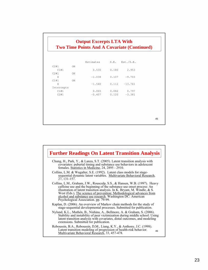
45
2.9530.1800.530C1#1C2#1 ON
-13.7610.112-1.540XC1#1 ON
-9.7030.107-1.038XC2#1 ON
-3.3810.120-0.407C2#10.797
Intercepts0.0820.065C1#1
Output Excerpts LTA WithTwo Time Points And A Covariate (Continued)
Estimates S.E. Est./S.E.
46
Chung, H., Park, Y., & Lanza, S.T. (2005). Latent transition analysis with covariates: pubertal timing and substance use behaviors in adolescent females. Statistics in Medicine, 24, 2895 - 2910.
Collins, L.M. & Wugalter, S.E. (1992). Latent class models for stage-sequential dynamic latent variables. Multivariate Behavioral Research, 27, 131-157.
Collins, L.M., Graham, J.W., Rousculp, S.S., & Hansen, W.B. (1997). Heavy caffeine use and the beginning of the substance use onset process: An illustration of latent transition analysis. In K. Bryant, M. Windle, & S. West (Eds.), The science of prevention: Methodological advances from alcohol and substance use research. Washington DC: American Psychological Association. pp. 79-99.
Kaplan, D. (2006). An overview of Markov chain methods for the study of stage-sequential developmental processes. Submitted for publication.
Nylund, K.L., Muthén, B., Nishina, A., Bellmore, A. & Graham, S. (2006). Stability and instability of peer victimization during middle school: Using latent transition analysis with covariates, distal outcomes, and modeling extensions. Submitted for publication.
Reboussin, B.A., Reboussin, D,M., Liang, K.Y., & Anthony, J.C. (1998). Latent transition modeling of progression of health-risk behavior. Multivariate Behavioral Research, 33, 457-478.
Further Readings On Latent Transition Analysis

24
47
Latent Transition Analysis Extensions
48
Latent Transition AnalysisAnd Intervention Studies
c1 c2
Tx
u2u1

25
49
VARIABLE:NAMES = u11-u15 u21-u25 tx;CATEGORICAL = u11-u15 u21-u25;CLASSES = cg(2) c1(2) c2(2);KNOWNCLASS = cg(tx=0 tx=1);
ANALYSIS: TYPE = MIXTURE MISSING;PROCESS = 2;STARTS = 100 20;
MODEL:%OVERALL%c2#1 ON c1#1@0
cg#1 (p0);[c2#1] (p1);
MODEL cg:%cg#1%c2#1 ON c1#1 (p2);%cg#2%c2#1 ON c1#1 (p3);
MODEL c1:%c1#1%[u11$1-u15$1*1] (1-5);%c1#2%[u11$1-u15$1*-1] (11-15);
Input For LTA With An Intervention
50
MODEL c2:%c2#1%[u21$1-u25$1*1] (1-5);
%c2#2%[u21$1-u25$1*-1] (11-15);
MODEL CONSTRAINT:NEW(p011 p012 p021 p022 p111 p112 p121 p122 lowlow highlow);!p0*, p1* contain probabilities for the 4 cells for control and !intervention groups !lowlow is the probability effect of intervention on staying in !the low class!highlow is the probability effect of intervention on moving from !high to low class!the effect is calculated as P(intervention)-P(control)p011 = exp(p0+p1+p2)/(exp(p0+p1+p2)+1);p012 = 1/(exp(p0+p1+p2)+1);p021 = exp(p0+p1)/(exp(p0+p1)+1);p022 = 1/(exp(p0+p1)+1);p111 = exp(p1+p3)/(exp(p1+p3)+1);p112 = 1/(exp(p1+p3)+1);p121 = exp(p1)/(exp(p1)+1);p122 = 1/(exp(p1)+1);lowlow = p111-p011;highlow = p121-p021;
OUTPUT:TECH1 PATTERNS;
PLOT:TYPE = PLOT3;

26
51
f1
c1
u11 . . . u1p
f2
c2
u21 . . . u2p
Time 1 Time 2
Factor Mixture Latent Transition AnalysisMuthen (2006)
Item probability
Item probability
Item Item
52
• 1,137 first-grade students in Baltimore public schools
• 9 items: Stubborn, Break rules, Break things, Yells at others,Takes others property, Fights, Lies, Teases classmates, Talksback to adults
• Skewed, 6-category items; dichotomized (almost never vs other)
• Two time points: Fall and Spring of Grade 1
• For each time point, a 2-class, 1-factor FMA was found best fitting
Factor Mixture Latent Transition Analysis:Aggressive-Disruptive Behavior In The Classroom

27
53
Factor Mixture Latent Transition Analysis:Aggressive-Disruptive Behavior In The Classroom
(Continued)
16,30640-8,012 FMA LTAfactors relatedacross time
17,44521-8,649 Conventional LTA
BIC# parametersLoglikelihoodModel
54
Factor Mixture Latent Transition Analysis:Aggressive-Disruptive Behavior In The
Classroom (Continued)
Estimated Latent Transition Probabilities, Fall to Spring
0.590.41High0.060.94LowHighLow
FMA-LTA0.830.17High0.070.93LowHighLow
Conventional LTA

28
55
Growth Modeling
56
(1) yti = η0i + η1i xt + εti
(2a) η0i = α0 + γ0 wi + ζ0i
(2b) η1i = α1 + γ1 wi + ζ1i
Individual Development Over Time
y1
w
y2 y3 y4
η0 η1
ε1 ε2 ε3 ε4
t = 1 t = 2 t = 3 t = 4
i = 1
i = 2
i = 3
y
x

29
57
Growth Modeling Frameworks/Software
Multilevel Mixed Linear
SEM
Latent Variable Modeling (Mplus)
(SAS PROC Mixed)(HLM)
58
Advantages Of Growth Modeling In A Latent Variable Framework
• Flexible curve shape• Individually-varying times of observation• Regressions among random effects• Multiple processes• Modeling of zeroes• Multiple populations• Multiple indicators• Embedded growth models• Categorical latent variables: growth mixtures

30
59
Growth Models WithCategorical Outcomes
60
The NIMH Schizophrenia Collaborative Study
• The Data—The NIMH Schizophrenia Collaborative Study (Schizophrenia Data)
• A group of 64 patients using a placebo and 249 patients on a drug for schizophrenia measured at baseline and at weeks one through six
• Variables—severity of illness, background variables, and treatment variable
• Data for the analysis—severity of illness at weeks one, two, four, and six and treatment

31
61
Placebo GroupDrug Group
Pro
porti
on
Week
1 2 3 4 5 6
0.0
0.2
0.4
0.6
0.8
1.0
Schizophrenia Data: Sample Proportions
62
illness1 illness2 illness4 illness6
drug
i s

32
63
Input For Schizophrenia Data Growth ModelFor Binary Outcomes With A Treatment Variable
i s | illness1@0 illness2@1 illness4@3illness6@5;
i s ON drug;
MODEL:
TYPE = MEANSTRUCTURE;ESTIMATOR = ML;!ESTIMATOR = WLSMV;
ANALYSIS:
NAMES ARE illness1 illness2 illness4 illness6drug; ! 0=placebo (n=64) 1=drug (n=249)
CATEGORICAL ARE illness1-illness6;
VARIABLE:
FILE IS schiz.dat; FORMAT IS 5F1;DATA:
Schizophrenia DataGrowth Model for Binary OutcomesWith a Treatment Variable and Scaling Factors
TITLE:
Alternative language:
i BY illness1-illness6@1;s BY illness1@0 illness2@1 illness4@3 illness6@5;[illness1$1 illness2$1 illness4$1 illness6$1] (1);[s];i s ON drug;!{illness1@1 illness2-illness6};
MODEL:
64
Tests Of Model Fit
LoglikelihoodHO Value -486.337
Information CriteriaNumber of Free Parameters 7Akaike (AIC) 986.674Bayesian (BIC) 1012.898Sample-Size Adjusted BIC 990.696
(n* = (n + 2) / 24)
Output Excerpts Schizophrenia Data Growth ModelFor Binary Outcomes With A Treatment Variable
n = 313
33
65
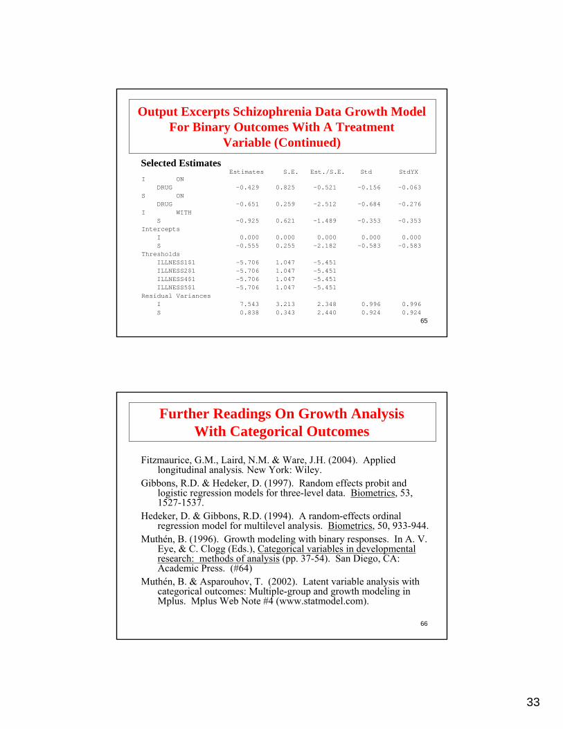
0.9960.9962.3483.2137.543IResidual Variances
-5.4511.047-5.706ILLNESS2$1-5.4511.047-5.706ILLNESS1$1
Thresholds
-5.4511.047-5.706ILLNESS4$1-5.4511.047-5.706ILLNESS5$1
0.9240.9242.4400.3430.838S
-0.583-0.583-2.1820.255-0.555S 0.0000.0000.0000.0000.000I
Intercepts-0.353-0.353-1.4890.621-0.925S
I WITH-0.276-0.684-2.5120.259-0.651DRUG
S ON-0.063-0.156-0.5210.825-0.429DRUG
I ONEstimates S.E. Est./S.E. Std StdYX
Selected Estimates
Output Excerpts Schizophrenia Data Growth ModelFor Binary Outcomes With A Treatment
Variable (Continued)
66
Fitzmaurice, G.M., Laird, N.M. & Ware, J.H. (2004). Applied longitudinal analysis. New York: Wiley.
Gibbons, R.D. & Hedeker, D. (1997). Random effects probit and logistic regression models for three-level data. Biometrics, 53, 1527-1537.
Hedeker, D. & Gibbons, R.D. (1994). A random-effects ordinal regression model for multilevel analysis. Biometrics, 50, 933-944.
Muthén, B. (1996). Growth modeling with binary responses. In A. V. Eye, & C. Clogg (Eds.), Categorical variables in developmental research: methods of analysis (pp. 37-54). San Diego, CA: Academic Press. (#64)
Muthén, B. & Asparouhov, T. (2002). Latent variable analysis with categorical outcomes: Multiple-group and growth modeling in Mplus. Mplus Web Note #4 (www.statmodel.com).
Further Readings On Growth Analysis With Categorical Outcomes

34
67
iu
iy sy
su
maleblackhispesfh123hsdrpcoll
qy
qu
y18 y19 y20 y24 y25
u18 u19 u20 u24 u25
neve
r
once
2 or
3 ti
mes
4 or
5 ti
mes
6 or
7 ti
mes
8 or
9 ti
mes
10 o
r mor
e tim
es
HD83
0
50
100
150
200
250
300
350
400
450
500
550
600
650
700
750
800
850
900
950
1000
1050
Cou
nt
Two-Part Growth Modeling:Frequency Of Heavy Drinking Ages 18 – 25
Olsen and Schafer (2001)neve
r
once
2 or
3 ti
mes
4 or
5 ti
mes
6 or
7 ti
mes
8 or
9 ti
mes
10 o
r mor
e tim
es
0
50
100
150
200
250
300
350
400
450
500
550
600
650
700
750
800
850
900
950
1000
1050
Cou
nt
neve
r
once
2 or
3 ti
mes
4 or
5 ti
mes
6 or
7 ti
mes
8 or
9 ti
mes
10 o
r mor
e tim
es
HD83
0
50
100
150
200
250
300
350
400
450
500
550
600
650
700
750
800
850
900
950
1000
1050
Cou
nt
68
Two-Part Growth Mixture Modeling
iu
iy sy
su
maleblackhispesfh123hsdrpcoll
qy
qu
y18 y19 y20 y24 y25
u18 u19 u20 u24 u25
cy
cu

35
69
Two-Part Modeling Extensions In Mplus
• Growth modeling• Distal outcome• Parallel processes• Trajectory classes (mixtures)• Multilevel
• Factor analysis• Mixtures
• Latent classes for binary and continuous parts may be incorrectly picked up as additional factors in conventionalanalysis
• Multilevel
70
Growth Mixture Modeling

36
71
Individual Development Over Time
y1
w
y2 y3 y4
η0 η1
ε1 ε2 ε3 ε4
t = 1 t = 2 t = 3 t = 4
(1) yti = η0i + η1i xt + εti
(2a) η0i = α0 + γ0 wi + ζ0i
(2b) η1i = α1 + γ1 wi + ζ1i
i = 1i = 2
i = 3
y
x
72
Mixtures And Latent Trajectory Classes
Modeling motivated by substantive theories of:
• Multiple Disease Processes: Prostate cancer (Pearson et al.)
• Multiple Pathways of Development: Adolescent-limited versus life-course persistent antisocial behavior (Moffitt), crime curves (Nagin), alcohol development (Zucker, Schulenberg)
• Subtypes: Subtypes of alcoholism (Cloninger, Zucker)

37
73
Example: Mixed-Effects Regression Models ForStudying The Natural History Of Prostate Disease
Source: Pearson, Morrell, Landis and Carter (1994), Statistics in Medicine
MIXED-EFFECT REGRESSION MODELS
Years Before Diagnosis Years Before Diagnosis
Figure 2. Longitudinal PSA curves estimated from the linear mixed-effects model for the group average (thick solid line) and for each individual in the study (thin solid lines)
Controls
BPH Cases
Local/RegionalCancers
Metastatic CancersPS
A L
evel
(ng/
ml)
0
4
8
12
16
20
24
28
32
36
40
44
0
4
8
12
16
04
8
0
4
8
15 10 5 015 10 5 0
74
Placebo Non-Responders, 55% Placebo Responders, 45%
Ham
ilton
Dep
ress
ion
Rat
ing
Scal
e
05
1015
2025
30
Baseli
ne
Wash-i
n
48 ho
urs
1 wee
k
2 wee
ks
4 wee
ks
8 wee
ks
0
5
10
15
20
25
30
05
1015
2025
30
Baseli
ne
Wash-i
n
48 ho
urs
1 wee
k
2 wee
ks
4 wee
ks
8 wee
ks
0
5
10
15
20
25
30
A Clinical Trial Of Depression Medication:
Two-Class Growth Mixture Modeling

38
75
Mat
h A
chie
vem
ent
Poor Development: 20% Moderate Development: 28% Good Development: 52%
69% 8% 1%Dropout:
7 8 9 10
4060
8010
0
Grades 7-107 8 9 10
4060
8010
0
Grades 7-107 8 9 10
4060
8010
0
Grades 7-10
Mplus Graphics For LSAY MathAchievement Trajectory Classes
76
Female
Hispanic
Black
Mother’s Ed.
Home Res.
Expectations
Drop Thoughts
Arrested
Expelled
Math7 Math8 Math9 Math10
High SchoolDropout
i s
c
LSAY Math Achievement Trajectory Classes

39
77
Growth Mixture Modeling Of Developmental Pathways
Outcome
Escalating
Early Onset
Normative
Agex
i
u
s
c
y1 y2 y3 y4
q
18 37
78
• New setting:
– Sequential, linked processes
• New aims:
– Using an earlier process to predict a later process– Early prediction of failing class
Application: General growth mixture modeling of first- andsecond-grade reading skills and their Kindergarten precursors;prediction of reading failure (Muthén, Khoo, Francis, Boscardin,1999). Suburban sample, n = 410.
General Growth Mixture Modeling With Sequential Processes
40
79
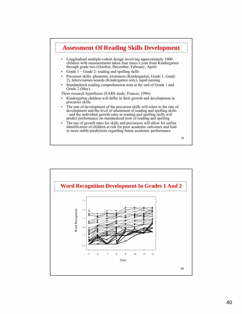
Assessment Of Reading Skills Development
• Longitudinal multiple-cohort design involving approximately 1000 children with measurements taken four times a year from Kindergarten through grade two (October, December, February, April)
• Grade 1 – Grade 2: reading and spelling skills• Precursor skills: phonemic awareness (Kindergarten, Grade 1, Grade
2), letters/names/sounds (Kindergarten only), rapid naming• Standardized reading comprehension tests at the end of Grade 1 and
Grade 2 (May).Three research hypotheses (EARS study; Francis, 1996):• Kindergarten children will differ in their growth and development in
precursor skills• The rate of development of the precursor skills will relate to the rate of
development and the level of attainment of reading and spelling skills – and the individual growth rates in reading and spelling skills will predict performance on standardized tests of reading and spelling
• The use of growth rates for skills and precursors will allow for earlier identification of children at risk for poor academic outcomes and lead to more stable predictions regarding future academic performance
80
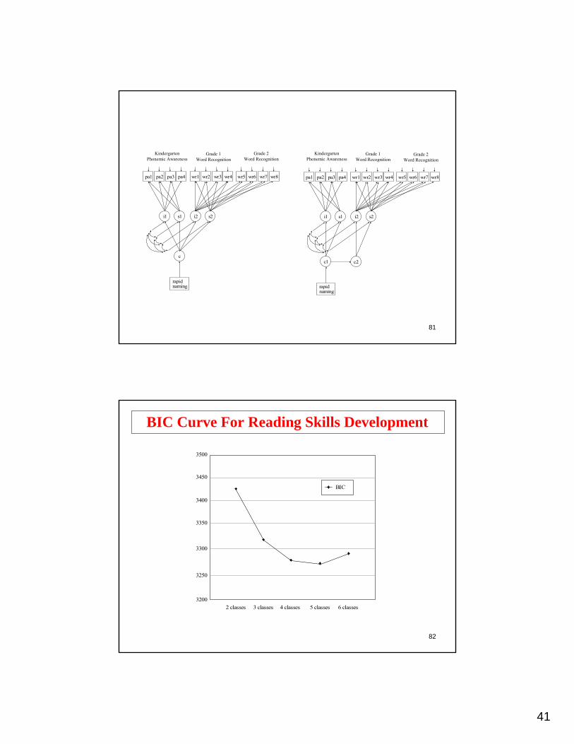
Word Recognition Development In Grades 1 And 2
Time
Wor
d R
ecog
nitio
n
-2-1
01
23
5 6 7 8 9 10 11 12
41
81
KindergartenPhonemic Awareness
Grade 1Word Recognition
Grade 2Word Recognition
i1
pa1 pa2 pa3 pa4 wr1 wr2 wr3 wr4 wr5 wr6 wr7 wr8
s1 i2 s2
c
rapidnaming
KindergartenPhonemic Awareness
Grade 1Word Recognition
Grade 2Word Recognition
i1
pa1 pa2 pa3 pa4 wr1 wr2 wr3 wr4 wr5 wr6 wr7 wr8
s1 i2 s2
c1
rapidnaming
c2
82
3500
3450
3400
3350
3300
3250
3200
BIC
2 classes 3 classes 4 classes 5 classes 6 classes
BIC Curve For Reading Skills Development

42
83
c#1-c#4 ON rnaming4;
FILE IS newran.dat;DATA:
TYPE = MIXTURE MISSING;ANALYSIS:
%OVERALL%i1 s1 | pa1@-3 pa2@-2 pa3@-1 pa4@0;i2 s2 | wr1@-7 wr2@-6 wr3@-5 wr4@-4 wr5@-3 wr6@-2
wr7@-1 wr8@0;
MODEL:
NAMES ARE gender eth wc pa1-pa4 wr1-wr8 l1-l4 s1 r1 s2 r2 rnaming1 rnaming2 rnaming3 rnaming4;USEVAR = pa1-wr8 rnaming4;MISSING ARE ALL (999);CLASSES = c(5);
VARIABLE:
TECH8;OUTPUT:
Growth mixture model for reading skills developmentTITLE:
Input For Growth Mixture ModelFor Reading Skills Development
84
Five Classes Of Reading Skills Development
21
0-1
-2-3
1 2 3 4 5 6 7 8 9 10 11 12
21
0-1
-2-3
Time Point Time Point
Kindergarten Growth (Five Classes)
Phonemic Awareness
Grades 1 and 2 Growth (Five Classes)
Word Recognition

43
85
Muthén, B. (2001). Second-generation structural equation modeling with a combination of categorical and continuous latent variables: New opportunities for latent class/latent growth modeling. In Collins, L.M. & Sayer, A. (Eds.), New methods for the analysis of change (pp. 291-322). Washington, D.C.: APA. (#82)
Muthén, B. (2001). Latent variable mixture modeling. In G. A. Marcoulides & R. E. Schumacker (eds.), New developments and techniques in structural equation modeling (pp. 1-33). Lawrence Erlbaum Associates. (#86)
Muthén, B. (2002). Beyond SEM: General latent variable modeling. Behaviormetrika, 29, 81-117. (#96)
Muthén, B. (2004). Latent variable analysis: Growth mixture modeling and related techniques for longitudinal data. In D. Kaplan (ed.), Handbook of quantitative methodology for the social sciences (pp. 345-368). Newbury Park, CA: Sage Publications. (#100)
Further Readings On Growth Mixture Modeling
86
Further Readings On Growth Mixture Modeling (Continued)
Muthén, B. & Asparouhov, T. (2006). Growth mixture analysis: Models with non-Gaussian random effects. Forthcoming in Fitzmaurice, G., Davidian, M., Verbeke, G. & Molenberghs, G. (eds.), Advances in Longitudinal Data Analysis. Chapman & Hall/CRC Press.
Muthén, B. & Muthén, L. (2000). Integrating person-centered and variable-centered analysis: growth mixture modeling with latent trajectory classes. Alcoholism: Clinical and Experimental Research, 24, 882-891. (#85)
Muthén, B. & Shedden, K. (1999). Finite mixture modeling with mixture outcomes using the EM algorithm. Biometrics, 55, 463-469. (#78)

44
87
Different treatment effects in different trajectory classes
Muthén, B., Brown, C.H., Masyn, K., Jo, B., Khoo, S.T., Yang, C.C.,Wang, C.P. Kellam, S., Carlin, J., & Liao, J. (2002). General growthmixture modeling for randomized preventive interventions. Biostatistics,3, 459-475.
Growth Mixtures In Randomized Trials
See also Muthen & Curran, 1997 for monotonic treatment effects
88
y2 y3 y4 y5y1 y6 y7
i s q
Txc
ANCOVA Growth Mixture Model
y1 y7
Tx
Modeling Treatment Effects
• GMM: treatment changes trajectory shape

45
89Figure 1. Path Diagrams for Models 1 - 3
y
η
Ι
c
Model 1
y
η
Ι
c
u
Model 2
y1
η1
Ι
c1
Model 3
y2
η2
c2
90Figure 6. Estimated Mean Growth Curves and Observed Trajectories for
4-Class model 1 by Class and Intervention Status
High Class, Control Group
Grades 1-7
TOC
A-R
12
34
56
12
34
56
1F 1S 2F 2S 3S 4S 5S 6S 7S
High Class, Intervention Group
Grades 1-7
TOC
A-R
12
34
56
12
34
56
1F 1S 2F 2S 3S 4S 5S 6S 7S
Medium Class, Control Group
Grades 1-7
TOC
A-R
12
34
56
12
34
56
1F 1S 2F 2S 3S 4S 5S 6S 7S
Medium Class, Intervention Group
Grades 1-7
TOC
A-R
12
34
56
12
34
56
1F 1S 2F 2S 3S 4S 5S 6S 7S
Low Class, Control Group
Grades 1-7
TOC
A-R
12
34
56
12
34
56
1F 1S 2F 2S 3S 4S 5S 6S 7S
Low Class, Intervention Group
Grades 1-7
TOC
A-R
12
34
56
12
34
56
1F 1S 2F 2S 3S 4S 5S 6S 7S
LS Class, Control Group
Grades 1-7
TOC
A-R
12
34
56
12
34
56
1F 1S 2F 2S 3S 4S 5S 6S 7S
LS Class, Intervention Group
Grades 1-7
TOC
A-R
12
34
56
12
34
56
1F 1S 2F 2S 3S 4S 5S 6S 7S

46
91
TOC
A-R
3-Class Model 1
1F 1S 2F 2S 3S 4S 5S 6S 7SGrades 1 - 7
High Class, 15%Medium Class, 44%Low Class, 19%
ControlIntervention
LS Class, 22%
BIC=3394Entropy=0.80
4-Class Model 1
TOC
A-R
1F 1S 2F 2S 3S 4S 5S 6S 7SGrades 1 - 7
High Class, 14%Medium Class, 50%Low Class, 36%ControlIntervention
BIC=3421Entropy=0.83
92
3-Class Model Estimated Mean Class TrajectoriesAnd Posterior Probability Weighted Means, Control Group
1F 1S 2F 2S 3S 4S 5S 6S 7SGrades 1 - 7
Class 1 = 14%Class 2 = 50%Class 3 = 36%
TOC
A-R
TOC
A-R
1F 1S 2F 2S 3S 4S 5S 6S 7SGrades 1 - 7
Class 1 = 14%Class 2 = 50%Class 3 = 36%
3-Class Model Estimated Mean Class TrajectoriesAnd Posterior Probability Weighted Means, Intervention Group

47
93
tx = (intngrp==4);DEFINE:
FILE IS toca.dat;DATA:
TYPE = MIXTURE MISSING;ANALYSIS:%OVERALL%ac bc qc | sctaa11f@0 [email protected] sctaa12f@1 [email protected] [email protected] [email protected] [email protected] [email protected] [email protected];qc@0; bc qc ON tx;sctaa11f WITH sctaa11s; sctaa12f WITH sctaa12s;
MODEL:
NAMES ARE sctaa11f sctaa11s sctaa12f sctaa12s sctaa13ssctaa14s sctaa15s sctaa16s sctaa17s intngrp;MISSING ARE ALL (999);USEVARIABLES ARE sctaa11f-sctaa17s tx;CLASSES = c(3);
VARIABLE:
growth mixtures in randomized trialsTITLE:
Input For Growth MixturesIn Randomized Trials
94
%c#1%[ac*3 bc qc]; bc qc ON tx;%c#2%[ac*2 bc qc]; bc qc ON tx;%c#3%[ac*1 bc qc]; bc qc ON tx;ac sctaa11f-sctaa17s;
Input For Growth MixturesIn Randomized Trials (Continued)

48
95
Randomized Trials With Non-Compliance
96
Randomized Trials With NonCompliance• Tx group (compliance status observed)
– Compliers– Noncompliers
• Control group (compliance status unobserved)– Compliers– NonCompliers
Compliers and Noncompliers are typically not randomly equivalentsubgroups.
Four approaches to estimating treatment effects:1. Tx versus Control (Intent-To-Treat; ITT)2. Tx Compliers versus Control (Per Protocol)3. Tx Compliers versus Tx NonCompliers + Control (As-Treated)4. Mixture analysis (Complier Average Causal Effect; CACE):
• Tx Compliers versus Control Compliers• Tx NonCompliers versus Control NonCompliers
CACE: Little & Yau (1998) in Psychological Methods

49
97
CACE Estimation Via Mixture Modeling AndML Estimation In Mplus
The latent classes of people are principal strataStraightforward to add covariates for y and for c. Many extensions possible.
c
y
Z
u
98
Randomized Trials with NonCompliance: ComplierAverage Causal Effect (CACE) Estimation
c
y
Txx
UG Ex 7.23Ex 7.24

50
99
TRAINING DATATraining data can be used when latent class membership is known forcertain individuals in the sample.
Training data must include one variable for each latent class. Eachindividual receives a value of 0 or 1 for each class variable. A zeroindicates that the individual is not allowed to be in the class. A oneindicates that the individual is allowed to be in the class.
CACE Application
With CACE models, there are two classes, compliers and noncompliers.The treatment group has known class membership. The control groupdoes not. Therefore, the training data is as follows:
10Treatment Group NonCompliers01Treatment Group Compliers11Control Group
Class 2 Non-Compliers
Class 1Compliers
100
JOBS Data
The JOBS data are from a Michigan University Prevention ResearchCenter study of interventions aimed at preventing poor mental health of unemployed workers and promoting high quality of reemployment. The intervention consisted of five half-day training seminars that focused on problem solving, decision making group processes, and learning and practicing job search skills. The control group received a booklet briefly describing job search methods and tips. Respondents wererecruited from the Michigan Employment Security Commission. After a series of screening procedures, 1801 were randomly assigned totreatment and control conditions. Of the 1249 in the treatment group, only 54% participated in the treatment.
The variables collected in the study include depression scores and outcome measures related to reemployment. Background variables include demographic and psychosocial variables.
51
101
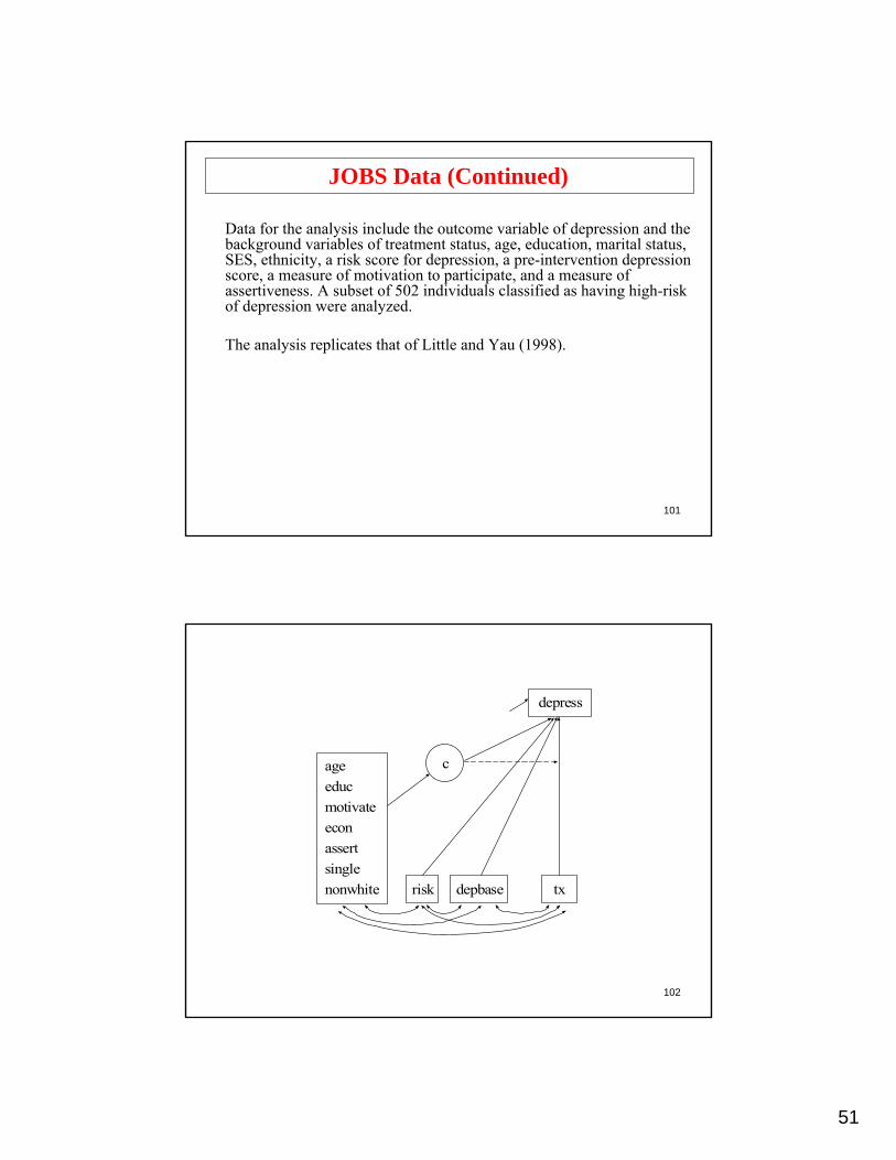
JOBS Data (Continued)
Data for the analysis include the outcome variable of depression and the background variables of treatment status, age, education, marital status, SES, ethnicity, a risk score for depression, a pre-intervention depression score, a measure of motivation to participate, and a measure of assertiveness. A subset of 502 individuals classified as having high-risk of depression were analyzed.
The analysis replicates that of Little and Yau (1998).
102
c
depress
depbase txrisk
ageeducmotivateeconassertsinglenonwhite

52
103
Input For Complier Average Causal Effect(CACE) Model
TYPE = MIXTURE;ANALYSIS:
TECH8;OUTPUT:
%OVERALL%
depress ON Tx risk depbase;c#1 ON age educ motivate econ assert single nonwhite;
%C#2% !c#2 is the noncomplier class (noshows)
[depress];
depress ON Tx@0;
MODEL:
NAMES ARE depress risk Tx depbase age motivate educ assert single econ nonwhite x10 c1 c2;
USEV ARE depress risk Tx depbase age motivate educ assert single econ nonwhite c1-c2;
CLASSES = c(2);TRAINING = c1-c2;
VARIABLE:
FILE IS wjobs.dat;DATA:
Complier Average Causal Effect (CACE) estimation in a randomized trial.
TITLE:
104
Tests Of Model FitLoglikelihood
H0 Value -729.414
Information Criteria
Number of Free Parameters 14Akaike (AIC) 1486.828Bayesian (BIC) 1545.888Sample-Size Adjusted BIC 1501.451
(n* = (n + 2) / 24)Entropy 0.727
Output Excerpts Complier Average Causal Effect(CACE) Model

53
105
Output Excerpts Complier Average Causal Effect(CACE) Model (Continued)
Model ResultsFINAL CLASS COUNTS AND PROPORTIONS OF TOTAL SAMPLE SIZE
0.54170271.93488Class 10.45830230.06512Class 2
CLASSIFICATION OF INDIVIDUALS BASED ON THEIR MOST LIKELY CLASS MEMBERSHIP
Class Counts and Proportions
0.55378278Class 10.44622224Class 2
Average Latent Class Probabilities for Most Likely Latent Class Membership (Row) by Latent Class (Column)
0.1000.900Class 10.9030.097Class 2
21
106
Output Excerpts Complier Average Causal Effect(CACE) Model (Continued)
Model Results (Continued)
6.068.2991.812DEPRESSIntercepts
Est./S.E.S.E.Estimates
.037
.181
.247
.130 -2.378-.310TXDepress ON
-8.077-1.463DEPBASE3.685.912RISK
Residual Variances13.742.506DEPRESS
Class 1
54
107
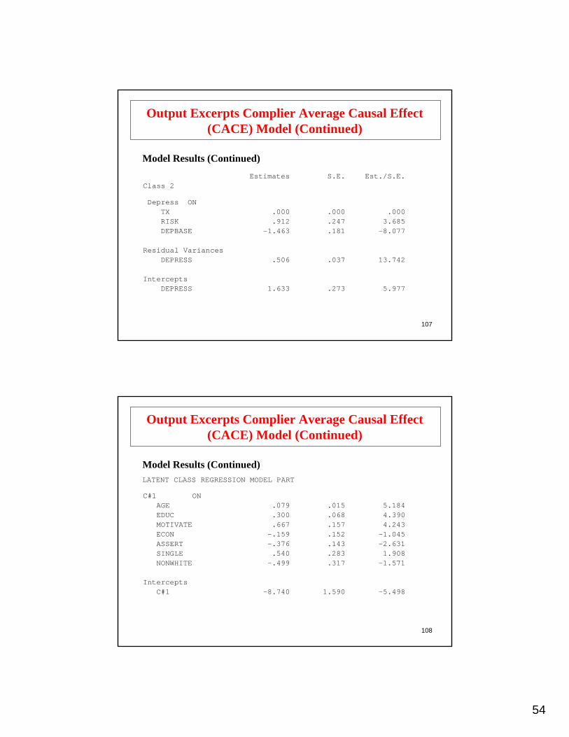
Output Excerpts Complier Average Causal Effect(CACE) Model (Continued)
Model Results (Continued)
5.977.2731.633DEPRESSIntercepts
Est./S.E.S.E.Estimates
.037
.181
.247
.000 .000.000TXDepress ON
-8.077-1.463DEPBASE3.685.912RISK
Residual Variances13.742.506DEPRESS
Class 2
108
Output Excerpts Complier Average Causal Effect(CACE) Model (Continued)
Model Results (Continued)LATENT CLASS REGRESSION MODEL PART
-5.4981.590-8.740C#1
C#1 ON
.317
.283
.143
.152
.157
.068
.015
-1.045-.159ECON4.243.667MOTIVATE4.390.300EDUC
1.908.540SINGLE-2.631-.376ASSERT
-1.571-.499NONWHITE
Intercepts
5.184.079AGE

55
109
Angrist, J.D., Imbens, G.W., Rubin, D.B. (1996). Identification of causal effects using instrumental variables. Journal of the American Statistical Association, 91, 444-445.
Jo, B. (2002). Estimation of intervention effects with noncompliance: Alternative model specifications. Journal of Educational and Behavioral Statistics, 27, 385-409.
Jo, B. (2002). Statistical power in randomized intervention studies with noncompliance. Psychological Methods, 7, 178-193.
Jo, B., Asparouhov, T., Muthén, B., Ialongo, N. & Brown, H. (2007). Cluster randomized trials with treatment noncompliance. Acceptedfor publication in Psychological Methods.
Little, R.J. & Yau, L.H.Y. (1998). Statistical techniques for analyzing data from prevention trials: treatment of no-shows using Rubin's causal model. Psychological Methods, 3, 147-159.
Further Readings OnCACE
110
Causal Inference

56
111
Causal Inference Concepts
• Potential outcomes
• Principal Stratification
• Finite mixtures
112
Potential Outcomes Framework
• Treatment variable X (e.g., X dichotomous with X=1 or X=0)
• Observed outcome Y, potential outcome variables Y(1), Y(0)
• Observed outcome under selected trmt x equals potential outcome under trmt assignment X=x : yi = yi(x) if xi = x
ACEMeans
yN = yN(1)yN(1)- yN(0)yN(0)yN(1)xN = 1N………………
y2 = y2(0)y2(1)- y2(0)y2(0)y2(1)x2 = 02
y1 = y1(1)y1(1)- y1(0)y1(0)y1(1)x1 = 11
YCausal EffectY(0)Y(1)XSubject #

57
113
Causal Inference And Non-Compliance
114
Causal Effects: The AIR (1996) Vietnam Draft Example
Angrist, Imbens & Rubin (1996) in JASA • Conscription into the military randomly allocated via
draft lottery
TREATMENT TAKEN
D
TREATMENT
ASSIGNMENTZ Y
OUTCOME

58
115
Causal Effects: The AIR (1996) Vietnam Draft Example (Continued)
• Z: treatment assignment (draft status) • Z = 1: assigned to serve in the military (for low lottery numbers)• Z = 0: not assigned to serve (for high lottery numbers)
• D: treatment taken (veteran status)• D = 1: served in the military
• D = 0: did not serve in the military
• Y: health outcome (mortality after discharge) • Note that D is not always = Z
• avoid the draft (or deferred for medical reasons); non-compliance: Z = 1, D=0
• volunteer for military service: Z = 0, D = 1
116
Causal Effect Of Z On Y, Yi(1, Di(1)) – Yi(0, Di(0)), For The Population Of Units Classified By Di(0) And Di(1)
Yi(1, 1) – Yi(0, 1) = 0Always-taker (πa ; µ1a, µ0a)
Yi(1, 1) – Yi(0, 0) = Yi(1) – Yi(0)Complier (πc ; µ1c, µ0c)
1
Yi(1, 0) – Yi(0, 1) = − (Yi(1) – Yi(0))Defier (π = 0)
Yi(1, 0) – Yi(0, 0) = 0Never-taker (πn ; µ1n, µ0n)
0Di(1)10
Di(0)
(12)DDE
DYDYE DDYYEii
iiiiiiii )]0()1([
)])0(,0())1(,1([]1)0()1(|))0()1([(−−
==−−
Average causal effect for compliers
Or, µ1c – µ0c = (µ1 – µ0 )/πc
Z Y is attributed to D Y under the exclusion restriction

59
117
• Mixture of 3 latent classes. Identification of parameters. Mixture means:µ1 = πc µ1c + π n µ1n + πa µ1a.µ0 = πc µ0c + π n µ0n + πa µ0a.µ1 – µ0 = πc (µ1c – µ0c) + πn × 0 + πa × 0
• Average causal effectµ1c – µ0c = (µ1 – µ0 )/πc
• Estimated average causal effect
wherepc+a is the proportion in the treatment group who take the treatmentpa is the proportion in the control group who take the treatment
In JOBS (Little & Yau, 1998), there are no always-takers (could not get into the seminars if not assigned), so
pa = 0
which is the Bloom (1984) IV estimate (the less compliance, the more attenuated the treatment and the more you upweight the mean difference).
),/()( 01 aac ppyy −− +
,/)( 01 cpyy −
Causal Effect of D Y Continued
118
Analysis With Missing Data

60
119
Analysis With Missing Data
Used when individuals are not observed on all outcomes in theanalysis to make the best use of all available data and to avoidbiases in parameter estimates, standard errors, and tests of model fit.
Types of Missingness
• MCAR -- missing completely at random• Variables missing by chance• Missing by randomized design• Multiple cohorts assuming a single population
• MAR -- missing at random• Missingness related to observed variables• Missing by selective design
• Non-Ignorable• Missingness related to values that would have been observed• Missingness related to latent variables
120
Estimation With Missing Data
Types of Estimation (Little & Rubin, 2002)
• Estimation using listwise deleted sample• When MCAR is true, parameter estimates and s.e.’s are
consistent but estimates are not efficient• When MAR is true but not MCAR, parameter estimates and
s.e.’s are not consistent• Maximum likelihood using all available data
• When MCAR or MAR is true, parameter estimates and s.e.’sare consistent and estimates are efficient
• Imputation• Mean and regression imputation – underestimation of
variances and covariances• Multiple imputation using all available data – a Bayesian
approach – credibility intervals are Bayesian justifiable under MCAR and MAR
• Pattern-mixture – used for non-ignorable missingness

61
121
Weighted Least Squares Estimation With Missing Data
Weighted least squares for categorical and censored outcomes
• Assumes MCAR when there are no covariates
• Allows MAR when missingness is a function of covariates
122
MCAR: Missing By Design
η
y2
y3
y1
η
y2
y3
y1
y1 y2 y3 η

62
123
Two-Cohort Growth Model
η0
y7
η1
y8 y9 y10 y11 y12
t = 0 t = 1 t = 2 t = 3 t = 4 t = 5
η0
y7
η1
y8 y9 y10 y11 y12
124
MAR
x
y
L H
yi = α + βxi + ζi
E(ζ) = 0, V(ζ) = E(x) = μx, V(x) =
2ζσ
2xσ
▫ Data Matrix:
Complete DataGroup
Missing Data
x y
nH
nL

63
125
Missing At Random (MAR): Missing On y In Bivariate Normal Case
xi / (nL + nH) =nL + nH
i = 1
nL xL + nH xHμx = Σ nL + nH
, (52)
nL + nH
(xi - μx)2 / (nL + nH)i = 1
σxx = Σ . (53)
126
estimated by the complete-data (listwise present) sample (sample size nH)
α = y – β x , (55)β = syx / sxx , (56)
σζζ = syy – / sxx . (57)2yxs
This gives the ML estimates of μy and σyy, adjusting the complete-data sample statistics:
μy = α + β μx = y + β (μx – x), (58)
σyy = σζζ + β2 σxx = syy + β2 (σxx – sxx). (59)
Missing At Random (MAR): Missing On y In Bivariate Normal Case (Continued)
Consider the regressionyi = α + β xi + ζi (54)

64
127
Correlates Of Missing Data• MAR is more plausible when the model includes covariates
influencing missing data
• Correlates of missing data may not have a “causal role” in the model, i.e. not influencing dependent variables, in which case including them as covariates can bias model estimates• Multiple imputation (Bayes; Schafer, 1997) with two
different sets of observed variables− Imputation model− Analysis model
• Modeling (ML)− Including missing data correlates not as x variables but as
“y variables,” freely correlated with all other observed variables
Recent overview in Schafer & Graham (2002).
128
Missing On X
• Regular modeling concerns the conditional distribution
[y | x] (1)
that is, as in regular regression the marginal distribution of [x] is not involved. This is fine if there is no missing on x in which case considering
[y | x]
gives the same estimates as (Joreskog & Goldberger, 1975) considering the joint distribution
[y, x] = [y | x] [x]

65
129
Missing On X (Continued)
• With missing on x, ML under MAR must make a distributional assumption about [x], typically normality. The modeling then concerns
[y, x] = [y | x] [x] (2)
which with missing on [x] is an expanded model that makes stronger assumptions as compared to (1).
• The LHS of (2) shows that y and x are treated the same -they are both “y variables” in Mplus terminology. This is the default in Mplus when all y’s are continuous. In other cases, x’s can be turned into “y’s” e.g. by the model statement
x1-xq;
130
Technical Aspects Of Ignorable Missing Data:ML Under MAR
Likelihood: log [yi | xi]. (87)i = 1Ση
With missing data on y, the ith term of (87) expands into[yi , yi , mi | xi], (88)
where mi is a 0/1 indicator vector of the same length as yi .The likelihood focuses on the observed variables,
[yi , mi | xi] = [yi , yi | xi] [mi | yi yi , xi] dyi , (89)which, when assuming that missingness is not a function ofyi (that is, assuming MAR),
obs mis
obs obs mis obs mis mis
mis

66
131
= [yi ,yi | xi] dyi [mi | yi , xi], (90)= [yi | xi] [mi | yi , xi]. (91)
With distinct parameter sets in (91), the last term can be ignored and maximization can focus on the [yi | xi] term. This leads to the standard MAR ignorable missing data procedure.
obs mis mis obs
obs obs
obs
Technical Aspects Of Ignorable Missing Data:ML Under MAR (Continued)
132
AMPS DataThe data are taken from the Alcohol Misuse Prevention Study(AMPS). Forty-nine schools with a total of 2,666 studentsparticipated in the study. Students were measured seven timesstarting in the Fall of Grade 6 and ending in the Spring of Grade 12.
Data for the analysis include the average of three items related toalcohol misuse:
During the past 12 months, how many times did you
drink more than you planned to?feel sick to your stomach after drinking?get very drunk?
Responses: (0) never, (1) once, (2) two times,(3) three or more times
Four of the seven timepoints are studied: Fall Grade 6, SpringGrade 6, Spring Grade 7, and Spring Grade 8.

67
133
amover0 amover1 amover2 amover3
i s
134
Input For AMPS Growth Model With Missing Data
FILE IS amps.dat;DATA:
NAMES ARE caseidamover0 ovrdrnk0 illdrnk0 vrydrn0
amover1 ovrdrnk1 illdrnk1 vrydrn1
amover2 ovrdrnk2 illdrnk2 vrydrn2amover3 ovrdrnk3 illdrnk3 vrydrn3
amover4 ovrdrnk4 illdrnk4 vrydrn4
amover5 ovrdrnk5 illdrnk5 vrydrn5amover6 ovrdrnk6 illdrnk6 vrydrn6;
USEV = amover0 amover1 amover2 amover3;
MISSING = ALL (999);
VARIABLE:
AMPS growth model with missing dataTITLE:

68
135
Input For AMPS Growth Model With Missing Data (Continued)
PATTERNS SAMPSTAT MODINDICES STANDARDIZED;OUTPUT:
TYPE = MISSING H1;ANALYSIS:
i s | amover0@0 amover1@1 amover2@3 amover3*5;amover1-amover3 PWITH amover0-amover2;
MODEL:
136
Output Excerpts AMPS Growth ModelWith Missing Data
x8
x
x7
x
x6
xx
x5
xx4
x
xx3
xxx2
xxxx1
x
12
x
x
11
xx
10
xxx
9
x
15
xAMOVER3xxAMOVER2
AMOVER1AMOVER0
1413
Summary of DataNumber of patterns 15
SUMMARY OF MISSING DATA PATTERNS
114866916443
6237104
Frequency
15
131211
Pattern
208
641129
Frequency
10
876
Pattern
65
73143685
Frequency
5
321
Pattern
MISSING DATA PATTERNS
MISSING DATA PATTERN FREQIENCIES

69
137
Output Excerpts AMPS Growth ModelWith Missing Data (Continued)
COVARIANCE COVERAGE OF DATA
0.7530.7150.347AMOVER20.682
AMOVER3
0.610
AMOVER2
0.650
0.933
AMOVER1
0.314
0.4010.464
AMOVER0
AMOVER3
AMOVER1AMOVER0
Minimum covariance coverage value 0.100
PROPORTION OF DATA PRESENT
Covariance Coverage
138
Output Excerpts AMPS Growth ModelWith Missing Data (Continued)
Tests Of Model Fit
Chi-square Test of Model Fit
Value 0.011Degrees of Freedom 1P-Value 0.9177
RMSEA (Root Mean Square Error Of Approximation)
Estimate 0.00090 Percent C.I. 0.000 0.019Probability RMSEA <= .05 0.997

70
139AMOVER3 WITH
-0.146-0.146-2.2780.003-0.007WITHAMOVER1 WITH
-0.085-0.022-2.0100.011-0.022AMOVER0
S I
AMOVER2 WITH
S |0.0000.0000.0000.0000.000AMOVER0.1980.1090.0000.0001.000AMOVER1
0.5290.4260.0000.0001.000AMOVER30.6450.4260.0000.0001.000AMOVER20.7740.4260.0000.0001.000AMOVER10.9210.4260.0000.0001.000AMOVER0
-0.003-0.001-0.0500.027-0.001AMOVER2
0.0470.0172.5050.0070.017AMOVER1
0.8430.68014.6450.4266.244AMOVER30.4940.3270.0000.0003.000AMOVER2
I |
Model Results
Output Excerpts AMPS Growth ModelWith Missing Data (Continued)
Estimates S.E. Est./S.E. Std StdYX
140
Output Excerpts AMPS Growth ModelWith Missing Data (Continued)
Variances
0.0000.0000.0000.0000.000AMOVER30.0000.0000.0000.0000.000AMOVER20.0000.0000.0000.0000.000AMOVER10.0000.0000.0000.0000.000AMOVER0
0.5200.52011.8580.0050.057SIntercept
0.4690.46919.3910.0100.200I
1.0001.00012.8910.0140.182I1.0001.0005.3780.0020.012S
0.1400.0911.3400.0680.091AMOVER30.4330.19011.4610.0170.190AMOVER20.4060.12310.9500.0110.123AMOVER10.1520.0332.5090.0130.033AMOVER0
Means
Residual Variances

71
141
Output Excerpts AMPS Growth ModelWith Missing Data (Continued)
0.860AMOVER30.567AMOVER20.594AMOVER10.848AMOVER0
R-SquareVariableObserved
R-SQUARE
142
0.6
MARListwiseam
over
timepoint0 1 3 5
0
0.1
0.2
0.3
0.4
0.5
AMPS: Estimated Growth Curves

72
143
Outcome
Escalating
Early Onset
NormativeAge
i
y2 y3 y4
s
x c
y1
u1 u2 u3 u4
Growth Mixture ModelingWith Ignorable Missingness
144
Selection modeling: [y | x] [m | y, x]. Different approaches to [m | y, x]:
Little & Rubin (2002) book: overviewDiggle & Kenward (1994) in Applied Statistics:
using y, y* (non-ignorable dropout)Wu & Carroll (1988), Wu & Bailey (1989) in Biometrics:
using the slope s Frangakis & Rubin (1999) in Biometrika:
using a latent class variable c (compliance)Muthen, Jo, Brown (2003) in JASA:
using c and s (GMM)
Pattern-mixture modeling: [m | x] [y | m, x]
Little & Rubin (2002): overviewRoy (2003) in Biometrics:
using a latent class variable c (missing data patterns)
Non-Ignorable Missing DataModeling Approaches And References

73
145
Outcome
Escalating
Early Onset
NormativeAge
i
y2 y3 y4
s
x c
y1
u1 u2 u3 u4
Growth Mixture Modeling WithNon-Ignorable Missingness As A Function Of y
146
Outcome
Escalating
Early Onset
NormativeAge
i
y2 y3 y4
s
x c
y1
u1 u2 u3 u4
Growth Mixture Modeling WithNon-Ignorable Missingness As A Function Of s

74
147
Outcome
Escalating
Early Onset
NormativeAge
i
y2 y3 y4
s
x c
y1
u1 u2 u3 u4
Growth Mixture Modeling WithNon-Ignorable Missingness As A Function Of c
148
Outcome
Escalating
Early Onset
NormativeAge
i
y2 y3 y4
s
x cy
y1
u1 u2 u3 u4
cu
Growth Mixture Modeling WithNon-Ignorable Missingness As A Function Of cu

75
149
Hedeker, D. & Rose, J.S. (2000). The natural history of smoking: A pattern-mixture random-effects regression model. Multivariate applications in substance use research, J. Rose, L. Chassin, C. Presson & J. Sherman (eds.), Hillsdale, N.J.: Erlbaum, pp. 79-112.
Little, R.J., & Rubin, D.B. (2002). Statistical analysis with missing data. 2nd edition. New York: John Wiley & Sons.
Muthén, B., Kaplan, D., & Hollis, M. (1987). On structural equationmodeling with data that are not missing completely at random. Psychometrika, 42, 431-462. (#17)
Muthén, B., Jo, B. & Brown, H. (2003). Comment on the Barnard, Frangakis, Hill & Rubin article, Principal stratification approach to broken randomized experiments: A case study of school choice vouchers in New York City. Journal of the American Statistical Association, 98, 311-314.
Schafer, J.L. (1997). Analysis of incomplete multivariate data. London: Chapman & Hall.
Schafer, J.L & Graham, J. (2002). Missing data: Our view of the state of the art. Psychological Methods, 7, 147- 177.
Further Readings On Missing Data Analysis
150
Multilevel Growth Models
76
151
time ys i
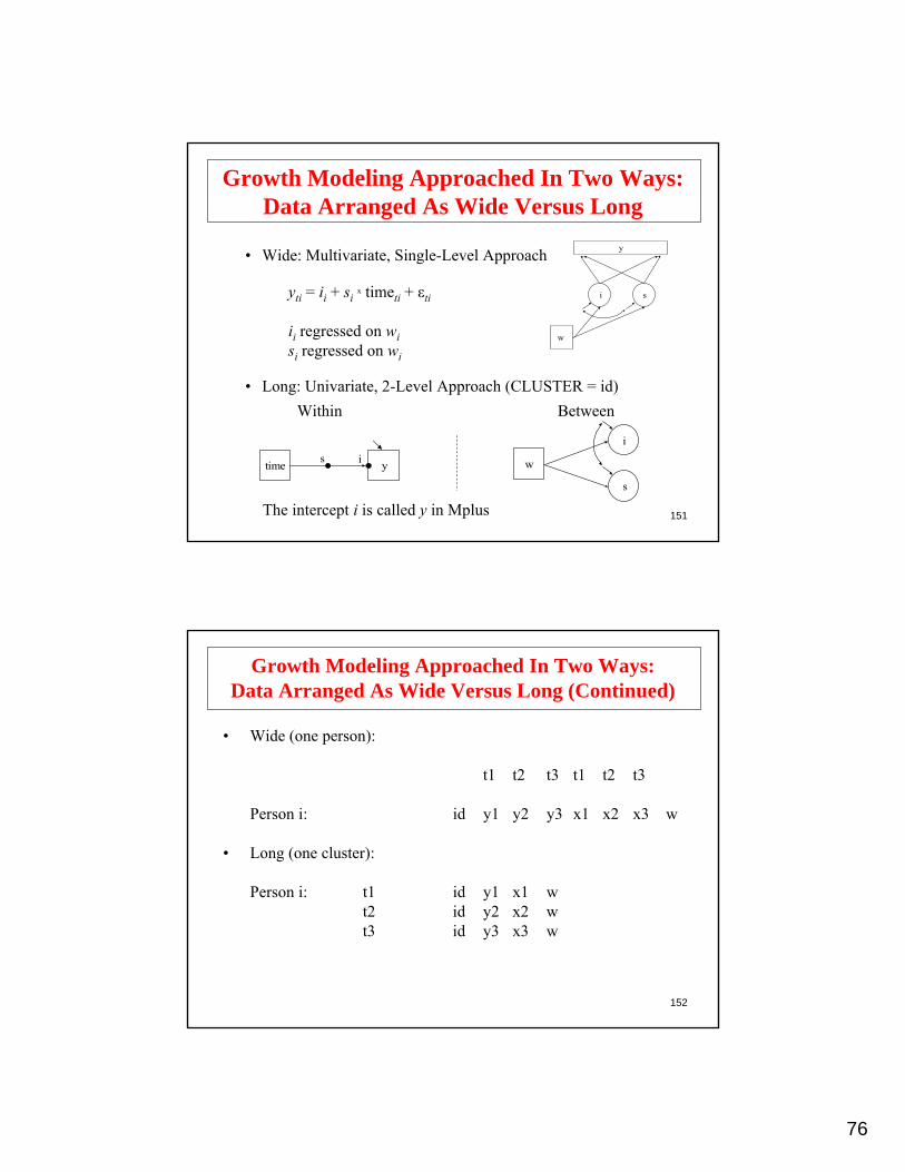
Growth Modeling Approached In Two Ways:Data Arranged As Wide Versus Long
yti = ii + six timeti + εti
ii regressed on wisi regressed on wi
• Long: Univariate, 2-Level Approach (CLUSTER = id)Within Between
y
i s
w
w
i
s
The intercept i is called y in Mplus
• Wide: Multivariate, Single-Level Approach
152
Growth Modeling Approached In Two Ways:Data Arranged As Wide Versus Long (Continued)
• Wide (one person):
t1 t2 t3 t1 t2 t3
Person i: id y1 y2 y3 x1 x2 x3 w
• Long (one cluster):
Person i: t1 id y1 x1 wt2 id y2 x2 wt3 id y3 x3 w

77
153
Time point t, individual i, cluster j.
ytij : individual-level, outcome variablea1tij : individual-level, time-related variable (age, grade)a2tij : individual-level, time-varying covariatexij : individual-level, time-invariant covariatewj : cluster-level covariate
Three-level analysis (Mplus considers Within and Between)
Level 1 (Within) : ytij = π0ij + π1ij a1tij + π2tij a2tij + etij , (1)
π 0ij = ß00j + ß01j xij + r0ij ,π 1ij = ß10j + ß11j xij + r1ij , (2)π 2tij = ß20tj + ß21tj xij + r2tij .
ß00j = γ000 + γ001 wj + u00j ,ß10j = γ100 + γ101 wj + u10j ,ß20tj = γ200t + γ201t wj + u20tj , (3)
ß01j = γ010 + γ011 wj + u01j ,ß11j = γ110 + γ111 wj + u11j ,ß21tj = γ2t0 + γ2t1 wj + u2tj .
Level 2 (Within) :
Level 3 (Between) :
Three-Level Modeling In Multilevel Terms
ib
iw
154
Within Between
iw
x
y1
sw
y2 y3 y4
ib
w
y1
sb
y2 y3 y4
Two-Level Growth Modeling(Three-Level Modeling)

78
155
Within
Between
LSAY Two-Level Growth Model
iw sw
mothed homeres
math7 math8 math9 math10
ib sb
mothed homeres
math7 math8 math9 math10
156
Input For LSAY Two-Level Growth ModelWith Free Time Scores And Covariates
FILE IS lsay98.dat;FORMAT IS 3f8 f8.4 8f8.2 3f8 2f8.2;
DATA:
NAMES ARE cohort id school weight math7 math8 math9 math10 att7 att8 att9 att10 gender mothed homeres; USEOBS = (gender EQ 1 AND cohort EQ 2);MISSING = ALL (999);USEVAR = math7-math10 mothed homeres;CLUSTER = school;
VARIABLE:
TYPE = TWOLEVEL;ESTIMATOR = MUML;
ANALYSIS:
LSAY two-level growth model with free time scores and covariates
TITLE:

79
157
SAMPSTAT STANDARDIZED RESIDUAL;OUTPUT
%WITHIN%iw sw | math7@0 math8@1math9*2 (1)math10*3 (2);iw sw ON mothed homeres;
%BETWEEN%ib sb | math7@0 math8@1math9*2 (1)math10*3 (2);ib sb ON mothed homeres;
MODEL:
Input For LSAY Two-Level Growth Model WithFree Time Scores And Covariates (Continued)
158
Output Excerpts LSAY Two-Level Growth ModelWith Free Time Scores And Covariates
304132136114
621
Summary of DataNumber of clusters 50
Size (s) Cluster ID with Size s
30240
1043430939
Average cluster size 18.627
Estimated Intraclass Correlations for the Y Variables
0.165MATH100.168MATH90.149MATH80.199MATH7
VariableIntraclassCorrelationVariable
IntraclassCorrelation
IntraclassCorrelationVariable

80
159
Tests Of Model Fit
Chi-square Test of Model FitValue 24.058*Degrees of Freedom 14P-Value 0.0451
CFI / TLICFI 0.997TLI 0.995
RMSEA (Root Mean Square Error Of Approximation)Estimate 0.028
SRMR (Standardized Root Mean Square Residual)Value for Between 0.048Value for Within 0.007
Output Excerpts LSAY Two-Level Growth ModelWith Free Time Scores And Covariates (Continued)
160
Output Excerpts LSAY Two-Level Growth ModelWith Free Time Scores And Covariates (Continued)
Model Results
Within Level
SW ON0.1730.1244.0310.2210.892HOMERES0.2260.2467.6650.2321.780MOTHED
IW ON0.3683.85316.0760.2233.589MATH100.2882.67015.2200.1632.487MATH90.1281.0730.0000.0001.000MATH8
SW BY
0.1760.1253.0470.0440.135HOMERES0.0450.0490.8360.0630.053MOTHED

81
161
Output Excerpts LSAY Two-Level Growth ModelWith Free Time Scores And Covariates (Continued)
SW WITH0.2730.2734.0440.5222.112IW
0.9030.90315.3333.06947.060IW0.22624.82911.1332.23024.829MATH100.16614.23712.5781.13214.237MATH90.17412.29813.7710.89312.298MATH80.19712.7488.8881.43412.748MATH7
Residual Variances0.2030.2616.7090.0390.261MOTHED
HOMERES WITH
1.0001.97028.6430.0691.970HOMERES1.0000.84117.2170.0490.841MOTHED
Variances0.9640.9643.8790.2861.110SW
162
Output Excerpts LSAY Two-Level Growth ModelWith Free Time Scores And Covariates (Continued)
Between Level
SB ON1.0112.1173.8761.8477.160HOMERES
-0.107-0.362-0.4742.587-1.225MOTHEDIB ON
0.1150.70416.0760.2233.589MATH100.1190.48815.2200.1632.487MATH90.0520.1960.0000.0001.000MATH8
SB BY
0.5750.5751.5380.2480.382IBSB WITH
0.0410.0860.0450.3730.017HOMERES1.4935.0731.5380.6470.995MOTHED
Estimates S.E. Est./S.E. Std StdYX

82
163
Output Excerpts LSAY Two-Level Growth ModelWith Free Time Scores And Covariates (Continued)
6.5093.10850.3750.0623.108HOMERES7.8382.30753.2770.0432.307MOTHED
Means
1.0000.0873.8010.0230.087MOTHED1.0000.2284.0660.0560.228HOMERES
Intercepts9.9099.90912.5122.67833.510IB0.8300.8300.2100.7760.163SB
0.1250.1250.8451.6901.428IB0.0671.3952.7670.5041.395MATH100.0060.1050.4930.2130.105MATH90.0390.5442.0330.2680.544MATH80.1532.0593.7320.5522.059MATH7
Residual Variances0.7330.1035.4880.0190.103MOTHED
HOMERES WITH
Variances-1.321-1.321-0.7130.071-0.051SB
164
Output Excerpts LSAY Two-Level Growth ModelWith Free Time Scores And Covariates (Continued)
R-SquareWithin Level
0.036SW
R-SquareLatentVariable
0.774MATH100.834MATH90.826MATH80.803MATH7
R-SquareObservedVariable
0.097IW

83
165
Output Excerpts LSAY Two-Level Growth ModelWith Free Time Scores And Covariates (Continued)
R-SquareBetween Level
0.23207E+01UndefinedSW
R-SquareLatentVariable
0.933MATH100.994MATH90.961MATH80.847MATH7
R-SquareObservedVariable
0.875IW
166
Muthén, B. (1997). Latent variable modeling with longitudinal and multilevel data. In A. Raftery (ed), Sociological Methodology (pp. 453-480). Boston: Blackwell Publishers. (#73)
Raudenbush, S.W. & Bryk, A.S. (2002). Hierarchical linear models: Applications and data analysis methods. Second edition. Newbury Park, CA: Sage Publications.
Snijders, T. & Bosker, R. (1999). Multilevel analysis. An introduction to basic and advanced multilevel modeling. Thousand Oakes, CA: Sage Publications.
Further Readings On Three-Level Growth Modeling

84
167
y1 y2 y3 y4
iw sws
Student (Within)
w
s ib sb
y1 y2 y3 y4
School (Between)
Multilevel Modeling With A RandomSlope For Latent Variables
168
Two-Level, Two-Part Growth ModelingWithin Between
y1 y2 y3 y4
iuw
iyw syw
u1 u2 u3 u4
x
suw
y1 y2 y3 y4
iub
iyb syb
u1 u2 u3 u4
w
sub

85
169
Multilevel Mixture Modeling
170
Individual level(Within)
Cluster level(Between)
Class-varying
y
c
x
c
w
y
tx
Two-Level Regression Mixture Modeling:Cluster-Randomized CACE

86
171
c
u2 u3 u4 u5 u6u1
x
f
c#1
w
c#2
Within Between
Two-Level Latent Class Analysis
172
Within
Between
c1
u11 . . . u1p
c2
u21 . . . u2p
c1#1 c2#2
Two-Level Latent Transition AnalysisAsparouhov & Muthen (2006)

87
173
Multilevel Growth Mixture Modeling
174
Mat
h A
chie
vem
ent
Poor Development: 20% Moderate Development: 28% Good Development: 52%
69% 8% 1%Dropout:
7 8 9 10
4060
8010
0
Grades 7-107 8 9 10
4060
8010
0
Grades 7-107 8 9 10
4060
8010
0
Grades 7-10
Growth Mixture Modeling:LSAY Math Achievement Trajectory ClassesAnd The Prediction Of High School Dropout

88
175mstrat
hsdrop
c
iw sw
math7 math8 math9 math10
math7 math9 math10
ib lunch
math8
hsdrop
C#1
C#2
female
hispanic
black
mother’s ed.
home res.
expectations
drop thoughts
arrested
expelled Within
Between
176
FILE = lsayfull_Dropout.dat;DATA:
NAMES = female mothed homeres math7 math8 math9 math10 expel arrest hisp black hsdrop expect lunch mstratdroptht7 schcode;!lunch = % of students eligible for full lunch!assistance (9th)!mstrat = ratio of students to full time math!teachers (9th)MISSING = ALL (9999);CATEGORICAL = hsdrop;CLASSES = c (3);CLUSTER = schcode;WITHIN = female mothed homeres expect droptht7 expel arrest hisp black;BETWEEN = lunch mstrat;
VARIABLE:
multilevel growth mixture model for LSAY math achievement
TITLE:
Input For A Multilevel Growth Mixture ModelFor LSAY Math Achievement

89
177
TYPE = PLOT3;SERIES = math7-math10 (s);
PLOT:
SAMPSTAT STANDARDIZED TECH1 TECH8;OUTPUT:
TYPE = MIXTURE TWOLEVEL MISSING;ALGORITHM = INTEGRATION;
ANALYSIS:
lunch = lunch/100;mstrat = mstrat/1000;
DEFINE:
Input For A Multilevel Growth Mixture ModelFor LSAY Math Achievement (Continued)
178
%WITHIN%
%OVERALL%
i s | math7@0 math8@1 math9@2 math10@3;
i s ON female hisp black mothed homeres expect droptht7 expel arrest;
c#1 c#2 ON female hisp black mothed homeres expect droptht7 expel arrest;
hsdrop ON female hisp black mothed homeres expect droptht7 expel arrest;
MODEL:
Input For A Multilevel Growth Mixture ModelFor LSAY Math Achievement (Continued)

90
179
%c#1%[i*40 s*1];math7-math10*20;i*13 s*3;
%c#2%[i*40 s*5];math7-math10*30;i*8 s*3;i s ON female hisp black mothed homeres expectdroptht7 expel arrest;
%c#3%[i*45 s*3];math7-math10*10;i*34 s*2;i s ON female hisp black mothed homeres expectdroptht7 expel arrest;
Input For A Multilevel Growth Mixture ModelFor LSAY Math Achievement (Continued)
180
%BETWEEN%
%OVERALL%
ib | math7-math10@1; [ib@0];
ib*1; hsdrop*1; ib WITH hsdrop;math7-math10@0;
ib ON lunch mstrat;
c#1 c#2 ON lunch mstrat;
hsdrop ON lunch mstrat;
%c#1%[hsdrop$1*-.3];
%c#2%[hsdrop$1*.9];
%c#3%[hsdrop$1*1.2];
Input For A Multilevel Growth Mixture ModelFor LSAY Math Achievement (Continued)

91
181
Power For Growth Models
182
Designing Future Studies: Power
• Computing power for growth models using Satorra-Saris (Muthén & Curran, 1997; examples)
• Computing power using Monte Carlo studies (Muthén & Muthén, 2002)
• Power calculation web site – PSMG• Multilevel power (Miyazaki & Raudenbush, 2000;
Moerbeek, Breukelen & Berger, 2000; Raudenbush, 1997; Raudenbush & Liu, 2000)
• School-based studies (Brown & Liao, 1999: Principles for designing randomized preventive trials)
• Multiple- (sequential-) cohort power• Designs for follow-up (Brown, Indurkhia, & Kellam,
2000)

92
183
Designing Future Studies: Power
χ2
H0 correct
5%
Type I error
H0 incorrect
P (Rejecting | H0 incorrect) = Power
Type II error
184
Power Estimation For Growth ModelsUsing Monte Carlo Studies
Muthén & Muthén (2002)

93
185
NAMES ARE y1-y4 x1 x2;NOBSERVATIONS = 500;NREPS = 500;SEED = 4533;CUTPOINTS = x2(1); MISSING = y1-y4;
MONTECARLO:
This is an example of a Monte Carlo simulation study for a linear growth model for a continuous outcome with missing data where attrition is predicted by time-invariant covariates (MAR)
TITLE:
Input Power Estimation For Growth ModelsUsing Monte Carlo Studies
186
x1-x2@1;[x1-x2@0];i s | y1@0 y2@1 y3@2 y4@3;[i*1 s*2];i*1; s*.2; i WITH s*.1;y1-y4*.5;i ON x1*1 x2*.5;s ON x1*.4 x2*.25;
MODEL POPULATION:
[y1-y4@-1];y1 ON x1*.4 x2*.2;y2 ON x1*.8 x2*.4;y3 ON x1*1.6 x2*.8;y4 ON x1*3.2 x2*1.6;
MODEL MISSING:
Input Power Estimation For Growth ModelsUsing Monte Carlo Studies (Continued)

94
187
TYPE = MISSING H1;ANALYSIS:
i s | y1@0 y2@1 y3@2 y4@3;MODEL:
[i*1 s*2];i*1; s*.2; i WITH s*.1;y1-y4*.5;i ON x1*1 x2*.5;s ON x1*.4 x2*.25;
TECH9;OUTPUT:
Input Power Estimation For Growth ModelsUsing Monte Carlo Studies (Continued)
188
Output Excerpts Power Estimation ForGrowth Models Using Monte Carlo Studies
Model Results
0.08770.0349
0.15700.0579
0.00750.0013
0.02410.0036
0.9380.936
0.9520.936
0.08650.0366
0.15540.0598
0.8300.24690.250X21.0000.39800.400X1
S ON
0.9080.50760.500X21.0001.00321.000X1
I ON
M. S. E. 95% %SigS.E.ESTIMATES
Average Cover CoeffStd. Dev.AveragePopulation

95
189
ReferencesAsparouhov, T. & Muthen, B. (2006). Multilevel mixture models. Forthcoming in
Hancock, G. R., & Samuelsen, K. M. (Eds.). (2007). Advances in latent variable mixture models. Charlotte, NC: Information Age Publishing, Inc.
Brown, E.C., Catalano, C.B., Fleming, C.B., Haggerty, K.P. & Abbot, R.D. (2005). Adolescent substance use outcomes in the Raising Healthy Children Project: A two-part latent growth curve analysis. Journal of Consulting and Clinical Psychology, 73, 699-710.
Dunn, G., Maracy, M., Dowrick, C., Ayuso-Mateos, J.L., Dalgard, O.S., Page, H., Lehtinen, V., Casey, P., Wilkinson, C., Vasquez-Barquero, J.L., & Wilkinson, G. (2003). Estimating psychological treatment effects from a randomized controlled trial with both non-compliance and loss to follow-up. British Journal of Psychiatry, 183, 323-331.
Jo, B. (2002). Statistical power in randomized intervention studies with noncompliance. Psychological Methods, 7, 178-193.
Jo, B., Asparouhov, T., Muthén, B., Ialongo, N. & Brown, H. (2007). Cluster randomized trials with treatment noncompliance. Accepted for publication in Psychological Methods.
190
References (continued)Jo, B., Asparouhov, T. & Muthén, B. (2007). Intention-to-treat analysis in cluster
randomized trials with noncompliance. Submitted for publication.Jo, B., Asparouhov, T., Muthén, B., Ialongo, N. & Brown, H. (2007). Cluster randomized trials with treatment noncompliance. Under review.
Kim, Y.K. & Muthén, B. (2007). Two-part factor mixture modeling: Application to an aggressive behavior measurement instrument. Submitted for publication.
Kreuter, F. & Muthen, B. (2007). Analyzing criminal trajectory profiles: Bridging multilevel and group-based approaches using growth mixture modeling.
Muthén, B. (2004). Latent variable analysis: Growth mixture modeling and related techniques for longitudinal data. In D. Kaplan (ed.), Handbook of quantitative methodology for the social sciences (pp. 345-368). Newbury Park, CA: Sage Publications.
Muthén, B. (2006). Latent variable hybrids: Overview of old and new models. Forthcoming in Hancock, G. R., & Samuelsen, K. M. (Eds.). (2007). Advances in latent variable mixture models. Charlotte, NC: Information Age Publishing, Inc.

96
191
Muthén, B. & Asparouhov, T. (2006). Growth mixture analysis: Models with non-Gaussian random effects. Forthcoming in Fitzmaurice, G., Davidian, M., Verbeke, G. & Molenberghs, G. (eds.), Advances in Longitudinal Data Analysis. Chapman & Hall/CRC Press.
Muthén, B. & Muthén, L. (2000). Integrating person-centered and variable-centered analyses: Growth mixture modeling with latent trajectory classes. Alcoholism: Clinical and Experimental Research, 24, 882-891.
Muthén, L. & Muthén, B. (2002). How to use a Monte Carlo study to decide on sample size and determine power. Structural Equation Modeling, 4, 599-620.
Muthén, B., Brown, C.H., Masyn, K., Jo, B., Khoo, S.T., Yang, C.C., Wang, C.P., Kellam, S., Carlin, J., & Liao, J. (2002). General growth mixture modeling for randomized preventive interventions. Biostatistics, 3, 459-475.
Nylund, K. (2007). Latent transition analysis: Modeling extensions and an application to peer victimization. Doctoral dissertation, University of California, Los Angeles.
References (continued)
192
Schaeffer, C.M., Petras, H., Ialongo, N., Poduska, J. & Kellam, S. (2003). Modeling growth in boys aggressive behavior across elementary school: Links to later criminal involvement, conduct disorder, and antisocial personality disorder. Developmental Psychology, 39, 1020-1035.
van Lier, P.A.C., Muthén, B., van der Sar, R.M. & Crijnen, A.A.M. (2004). Preventing disruptive behavior in elementary schoolchildren: Impact of a universal classroom-based intervention. Journal of Consulting and Clinical Psychology, 72, 467-478.
On Categorical Data Analysis:
Agresti, A. (2002). Categorical data analysis. Second edition. New York: John Wiley & Sons.
Agresti, A. (1996). An introduction to categorical data analysis. New York: Wiley.
Hosmer, D. W. & Lemeshow, S. (2000). Applied logistic regression. Second edition. New York: John Wiley & Sons.
Long, S. (1997). Regression models for categorical and limited dependent variables. Thousand Oaks: Sage.
References (continued)

97
193
References (continued)On Growth Modeling:
Bollen, K.A. & Curran, P.J. (2007). Latent curve models. A structural equation perspective. New York: Wiley & Sons.
Fitzmaurice, G.M., Laird, N.M. & Ware, J.H. (2004). Applied longitudinal analysis. New York: Wiley & Sons.
Raudenbush, S.W. & Bryk, A.S. (2002). Hierarchical linear models: Applications and data analysis methods. Second edition. Newbury Park, CA: Sage Publications.