Embed Size (px)
Citation preview

ANALYSIS OF NONLINEAR EFFECTS AND
THEIR MITIGATION IN FIBER-OPTIC
COMMUNICATION SYSTEMS

ANALYSIS OF NONLINEAR EFFECTS AND THEIR
MITIGATION IN FIBER-OPTIC COMMUNICATION SYSTEMS
BY
MAHDI MALEKIHA, B.Sc.
a thesis
submitted to the department of electrical & computer engineering
and the school of graduate studies
of mcmaster university
in partial fulfilment of the requirements
for the degree of
Master of Applied Science
c© Copyright by MAHDI MALEKIHA, August 2011
All Rights Reserved

Master of Applied Science (2011) McMaster University
(Electrical & Computer Engineering) Hamilton, Ontario, Canada
TITLE: ANALYSIS OF NONLINEAR EFFECTS AND THEIR
MITIGATION IN FIBER-OPTIC COMMUNICATION
SYSTEMS
AUTHOR: MAHDI MALEKIHA
B.Sc., (Electrical Engineering)
Isfahan University of Technology, Isfahan, Iran
SUPERVISOR: Dr. Shiva Kumar
NUMBER OF PAGES: xiv, 96
ii

To my beloved family, for your continued support and encouragment

Abstract
The rapid development of fiber optic communication systems requires higher trans-
mission data rate and longer reach. This thesis deals with the limiting factors in
design of long-haul fiber optic communication systems and the techniques used to
suppress their resulting impairments. These impairments include fiber chromatic dis-
persion, the Ker nonlinearity and nonlinear phase noise due to amplified spontaneous
emission.
In the first part of this thesis, we investigate the effect of amplified spontaneous
noise in quasi-linear systems. In quasi-linear systems, inline optical amplifiers change
the amplitude of the optical field envelope randomly and fiber nonlinear effects such
as self phase modulation (SPM) convert the amplitude fluctuations to phase fluctua-
tions which is known as nonlinear phase noise. For M-ary phase shift keying (PSK)
signals, symbol error probability is determined solely by the probability density func-
tion (PDF) of the phase. Under the Gaussian PDF assumption, the phase variance
can be related to the symbol error probability for PSK signals. We implemented the
simulation based on analytical phase noise variance and Monte-Carlo simulation, and
it is found that the analytical approximation is in good agreement with numerical
simulations. We have developed analytical expressions for the linear and nonlinear
phase noise variance due to SPM using second-order perturbation theory. It is found
iv

that as the transmission reach and/or lunch power increase, the variance of the phase
noise calculated using first order perturbation theory becomes inaccurate. However,
the variance calculated using second order perturbation theory is in good agreement
with numerical simulations. We have also showed that the analytical formula given
in this chapter for the variance of nonlinear phase noise can be used as a design tool
to investigate the optimum system design parameters such as average power and dis-
persion maps for coherent fiber optic systems based on phase shift keying due to the
fact that the numerical simulation of nonlinear Schrodinger (NLS) equation is time
consuming, however, the analytical method based on solving NLS equation using per-
turbation approximation is quite efficient and therefore the analytical variance can
be obtained more easily without requiring extensive computational efforts, and also
with fairly good accuracy.
In the second part of this thesis, an improved optical signal processing using highly
nonlinear fibers is studied. This technique, optical backward propagation (OBP), can
compensate for the fiber dispersion and nonlinearity using optical nonlinearity com-
pensators (NLC) and dispersion compensating fibers (DCF), respectively. In contrast,
digital backward propagation (DBP) uses the high-speed digital signal processing
(DSP) unit to compensate for the fiber nonlinearity and dispersion digital domain.
NLC imparts a phase shift that is equal in magnitude to the nonlinear phase shift
due to Fiber propagation, but opposite in sign. In principle, BP schemes could undo
the deterministic (bit-pattern dependent) nonlinear impairments, but it can not com-
pensate for the stochastic nonlinear impairments such as nonlinear phase noise. We
also introduced a novel inline optical nonlinearity compensation (IONC) technique.
Our Numerical simulations show that the transmission performance can be greatly
v

improved using OBP and IONC. Using IONC, the transmission reach becomes almost
twice of DBP. The advantage of OBP and IONC over DBP are as follows: OBP/IONC
can compensate the nonlinear impairments for all the channels of a wavelength di-
vision multiplexed system (WDM) in real time while it would be very challenging
to implement DBP for such systems due to its computational cost and bandwidth
requirement. OBP and IONC can be used for direct detection systems as well as for
coherent detection while they provide the compensation of dispersion and nonlinear-
ity in real time, but DBP works only for coherent detection and currently limited to
off-line signal processing.
vi

Acknowledgements
I would like to express my most sincere gratitude to my supervisor, Dr. Shiva Kumar.
It is an honor for me to study under his supervision. I appreciate all his contributions
of time, ideas, and funding to make my M.Sc. experience productive and stimulating.
The joy and enthusiasm he has for his research was contagious and motivational for
m, even during tough times in the M.Sc. pursuit.
I also would like to appreciate all colleagues of Photonic CAD Laboratory. They
have been a source of friendships as well as good advice and collaboration.
For this dissertation, I would like to thank my defense committee members: Dr.
Mohamed Bakr and Dr. Chih-Hung Chen for their time, interest, helpful comments
and insightful questions.
My time at McMaster was made enjoyable in large part due to the many friends
and groups that became a part of my life. I am grateful for time spent with roommates
and friends, and for many other people and memories.
Lastly, I would like to thank my family for all their love and encouragement. For
my parents who raised me with a love of science and supported me in all my pursuits.
And most of all for my loving, supportive, encouraging, and patient wife Mehrnoosh
whose faithful support during the final stages of this M.Sc. is so appreciated.
vii

viii

Notation and abbreviations
ASE Amplified Spontaneous Emission
BER Bit Error Rate
CD Chromatic Dispersion
DGD Differential Group Delay
DCF Dispersion-Compensating Fiber
DPSK Differential Phase-Shift Keying
PSK Phase-Shift Keying
QAM Quadrature Amplitude Modulation
FNL Fiber Nonlinearity
FFT Fast Fourier Transform
FWM Four-Wave Mixing
IFWM Intra-channel Four-Wave Mixing
XPM Cross-Phase Modulation
IXPM Intra-channel Cross-Phase Modulation
IONC Inline optical nonlinearity compensation
NLSE Nonlinear Schrodinger Equation
NPS Nonlinear Phase Shift PMD Polarization Mode Dispersion
PSP Principle State of Polarization
PDE Partial Differential Equationix

SPM Self-Phase Modulation
SMF Single Mode Fiber
SNR Signal-Noise Ratio
SSFS Split-Step Fourier Transform
DFS Dispersion-Shifted Fiber
WDM Wavelength-Division Multiplexing
EDFA Erbium-Doped Fiber Amplifier
OE Optical-to-Electrical
EO Electrical-to-Optical
GVD Group velocity Dispersion
ISI Inter-Symbol Interference
FP Forward propagation
DBP Digital Backward Propagation
OBP Optical Backward Propagation
NRZ Non-Return-to-Zero
NLC Nonlinearity Compensator
PRBS Pseudo-Random Bit Sequence
FEC Forward Error Correction
HNLF Highly Nonlinear Fiber
x

Contents
Abstract iv
Acknowledgements vii
Notation and abbreviations ix
1 Introduction 1
1.1 Evolution of Fiber-Optic Communications . . . . . . . . . . . . . . . 2
1.2 Thesis Contribution . . . . . . . . . . . . . . . . . . . . . . . . . . . . 9
2 Literature Background 11
2.1 Fiber Optic Communication Systems Impairments . . . . . . . . . . . 11
2.1.1 Chromatic Dispersion . . . . . . . . . . . . . . . . . . . . . . . 13
2.1.2 Fiber Kerr Nonlinearities . . . . . . . . . . . . . . . . . . . . . 16
2.2 Coherent Transmission Technology . . . . . . . . . . . . . . . . . . . 20
2.3 Dispersion Compensation Techniques . . . . . . . . . . . . . . . . . . 25
2.4 Backward Propagation . . . . . . . . . . . . . . . . . . . . . . . . . . 30
3 Analysis of Nonlinear Phase Noise in Fiber-Optic Communication
Systems 33
xi

3.1 Introduction . . . . . . . . . . . . . . . . . . . . . . . . . . . . . . . . 33
3.2 Quasi-Linear Systems . . . . . . . . . . . . . . . . . . . . . . . . . . . 36
3.3 Mathematical Derivation of Nonlinear Phase Noise Variance . . . . . 41
3.4 Numerical Simulations and Result . . . . . . . . . . . . . . . . . . . . 48
3.4.1 Variance of Nonlinear Phase Noise . . . . . . . . . . . . . . . 50
3.4.2 Optimizing Dispersion-Managed Fiber-Optic Systems . . . . . 53
3.5 Conclusion . . . . . . . . . . . . . . . . . . . . . . . . . . . . . . . . . 55
4 Optical Back Propagation for Fiber Optic Communications Using
Highly Nonlinear Fibers 57
4.1 Introduction . . . . . . . . . . . . . . . . . . . . . . . . . . . . . . . . 57
4.2 Theoretical Background on Backward Propagation . . . . . . . . . . . 59
4.2.1 Digital Backward Propagation . . . . . . . . . . . . . . . . . . 60
4.2.2 Optical Backward Propagation . . . . . . . . . . . . . . . . . 63
4.2.3 Inline Optical Nonlinearity Compensation Scheme . . . . . . . 68
4.3 Results and Discussion . . . . . . . . . . . . . . . . . . . . . . . . . . 69
4.3.1 Optical BP Vs. Digital BP . . . . . . . . . . . . . . . . . . . . 73
4.3.2 Sensitivity Analysis . . . . . . . . . . . . . . . . . . . . . . . . 77
4.4 Conclusion . . . . . . . . . . . . . . . . . . . . . . . . . . . . . . . . . 79
5 Conclusions and Future Work 80
A Linear, First-Order and Second-Order Nonlinear Solutions of NLS
Equation 83
A.1 Gauss-Hermite Solutions (Linear Solution) . . . . . . . . . . . . . . . 83
A.2 First-Order and Second-order Nonlinear Solutions . . . . . . . . . . . 86
xii

List of Figures
2.1 Schematic diagram of a coherent detection. . . . . . . . . . . . . . . . 20
2.2 Schematic diagram of the single-branch in-phase/quadrature coherent
receiver . . . . . . . . . . . . . . . . . . . . . . . . . . . . . . . . . . 23
2.3 A transmission span with a DCF. β21, L1 and β22, L2 are the GVD
parameter and length for SSMF and DCF, respectively . . . . . . . . 26
3.1 Schematic diagram of a coherent fiber optic system. . . . . . . . . . . 36
3.2 Typical dispersion and loss/gain profiles of a long-haul dispersion-
managed fiber-optic system. Pre- and post- compensation are not shown. 39
3.3 Schematic illustration of symmetric-SSF scheme . . . . . . . . . . . . 49
3.4 Optical power as a function of time at total transmission distance of
(a) 160 Km, (b) 480 Km and (c) 960 Km. The dotted, broken, and
solid lines show the numerical, first-order, and second-order solution,
respectively. |D| = 4 ps/nm.Km. . . . . . . . . . . . . . . . . . . . . 51
3.5 Phase variance dependence on the total length of the transmission line. 52
3.6 Dependence of phase variance on peak launch power. Ltot = 2400 Km
and |D| = 10 ps/nm.Km . . . . . . . . . . . . . . . . . . . . . . . . . 53
3.7 Dispersion-managed fiber link with pre- and post-dispersion compen-
sation. . . . . . . . . . . . . . . . . . . . . . . . . . . . . . . . . . . 54
xiii

3.8 Dependence of phase variance on peak launch power. Ltot = 2400 Km
and |D| = 10 ps/nm.Km . . . . . . . . . . . . . . . . . . . . . . . . . 55
4.1 Symmetric split-step Fourier method (SSFM) used to simulate the sig-
nal forward propagation through the transmission fiber. . . . . . . . 61
4.2 An ideal backward propagation for a single span. . . . . . . . . . . . 62
4.3 (a) Block diagram of a fiber-optic link with optical back propagation.
(b) Block diagram of NLC. . . . . . . . . . . . . . . . . . . . . . . . . 64
4.4 Optical field envelope vs normalized time. Ts = symbol interval, trans-
mission distance = 800 Km, peak launch power to fiber-link = 0 dBm
and nsp = 0. . . . . . . . . . . . . . . . . . . . . . . . . . . . . . . . 71
4.5 Bit error rate vs average launch power to the fiber-optic link. Trans-
mission distance = 800 Km. . . . . . . . . . . . . . . . . . . . . . . . 72
4.6 Bit error rate vs average launch power to the fiber-optic link for DBP,
perfect-DBP, OBP and inline nonlinearity compensation. . . . . . . . 73
4.7 Bit error rate vs transmission reach for DBP, perfect-DBP, OBP and
inline nonlinearity compensation (IONC). . . . . . . . . . . . . . . . . 74
4.8 Bit error rate vs average launch power to the fiber-optic link for DBP
schemes with 2, 4, 8, 16 sample per symbol. . . . . . . . . . . . . . . 75
4.9 Bit error rate vs nonlinearity coefficient of HNLF2. Transmission dis-
tance = 800 Km. . . . . . . . . . . . . . . . . . . . . . . . . . . . . . 76
4.10 Bit error rate vs dispersion standard deviation of HNLF1 and HNLF2.
(a) IONC Transmission distance = 1440 Km, (b) OBP Transmission
distance = 1040 Km. . . . . . . . . . . . . . . . . . . . . . . . . . . 78
xiv

Chapter 1
Introduction
A communication system transmits information from one place to another, whether
separated by a few kilometers or by transoceanic distances. Information is often car-
ried by an electromagnetic carrier wave whose frequency can vary from a few mega-
hertz to several hundred terahertz. In the virtually infinite broad electromagnetic
spectrum, there are only two windows that have been largely used for modern-day
broadband communications. The first window spans from the long-wave radio to
millimeter wave, or from 100 KHz to 300 GHz in frequency, whereas the second win-
dow lies in the infrared lightwave region, or from 30 THz to 300 THz in frequency.
The first window provides the applications that we use in our daily lives, including
broadcast radio and TV, wireless local area networks (LANs), and mobile phones.
These applications offer the first meter or first mile access of the information net-
works to the end user with broadband connectivity or the mobility in the case of
the wireless systems. Nevertheless, most of the data rates are capped below gigabit
per second (Gb/s) primarily due to the lack of the available spectrum in the RF
microwave range. In contrast, due to the enormous bandwidth over several terahertz
1

M.A.Sc. Thesis - MAHDI MALEKIHA McMaster - Electrical Engineering
(THz) in the second window, the lightwave systems can provide a staggering capacity
of 100 Tb/s and beyond. In fact, the optical communication systems, or fiber-optic
systems in particular, have become indispensable as the backbone of the modern-day
information infrastructure. While initial deployment of optical fiber was mainly for
long-haul or submarine transmission, lightwave systems are currently in almost all
metro networks. Fiber-to-the-premise (FTTP) and fiber-to-the-home (FTTH) are
being considered seriously in most parts of the world right now [1].
Optical communication systems have been deployed worldwide since 1980 and
have indeed revolutionized the technology behind telecommunications. Indeed, the
lightwave technology, together with microelectronics, is believed to be a major factor
in the advent of the information age.
1.1 Evolution of Fiber-Optic Communications
A point-to-point fiber-optic communication system, the simplest kind of lightwave
system, consists of a transmitter, followed by transmission channel (fiber), and then
a receiver. The evolution of fiber-optic communications has been promoted along with
the advent of the above three major components in a fiber communication system.
In 1960, the invention and the realization of laser [2] provided a coherent source for
transmitting information using lightwaves. After that, In 1966, Kao and Hockman
proposed the idea of using the optical fiber as the lightwave transmission medium
despite the fact that optical fiber at the time suffered unacceptable loss (over 1000
dB/Km). They argued that the attenuation in fibers available at the time was caused
by impurities, which could be removed. Their prophetic prediction of 20 dB/Km for
telecom-grade optical fiber was realized 5 years later by researchers from Corning
2

M.A.Sc. Thesis - MAHDI MALEKIHA McMaster - Electrical Engineering
[3]. In 1979, the low loss fiber was realized at the operating wavelength of 1550
nm [4] with a loss of 0.2 dB/Km. The simultaneous availability of stable optical
source (laser) and a low-loss optical fiber led to an extensive research efforts and
rapid development of fiber-optic communication systems, which can be grouped into
five distinct generations [5]. A commonly used figure of merit for point-to-point
communication systems is the bit rate-distance product, BL, where B is the bit
rate and L is the repeater spacing. In every generation, BL increases initially but
then begins to saturate as the technology matures. Each new generation brings a
fundamental change that helps to improve the system performance further.
The first-generation of lightwave systems operated near 800 nm and used GaAs
semiconductor lasers. They operated at a bit rate of 45 Mb/s and allowed repeater
spacings of up to 10 Km. The repeater spacing of the first-generation lightwave
systems was limited by fiber dispersion which lead to pulse-spreading at the operating
wavelength of 800 nm. In 1970s that the repeater spacing increased considerably by
operating the lightwave system in the wavelength region near 1300 nm, where optical
fibers exhibit minimum dispersion Furthermore, fiber loss is below 1 dB/Km. This
realization led to a worldwide effort for the development of InGaAsP semiconductor
lasers and detectors operating near 1300 nm. The second generation of fiber-optic
communication systems became available in the early 1980s, but the bit rate of early
systems was limited to below 100 Mb/s because of intermodal dispersion in multimode
fibers. This limitation was overcome by the use of single-mode fibers. By 1987,
second-generation lightwave systems, operating at bit rates of up to 1.7 Gb/s with a
repeater spacing of about 50 Km, were commercially available.
The repeater spacing of the second-generation lightwave systems was limited by
3

M.A.Sc. Thesis - MAHDI MALEKIHA McMaster - Electrical Engineering
the fiber losses at the operating wavelength of 1300 nm (typically 0.5 dB/km). Losses
of silica fibers become minimum near 1550 nm. Indeed, a 0.2 dB/Km loss was realized
in 1979 in this spectral region. The drawbacks of 1550 nm systems were a large fiber
dispersion near 1550 nm, and the conventional InGaAsP semiconductor lasers could
not be used because of pulse spreading occurring as a result of simultaneous oscillation
of several longitudinal modes. The dispersion problem can be overcome either by
using dispersion-shifted fibers designed to have minimum dispersion near 1550 nm
or by limiting the laser spectrum to a single longitudinal mode. For a dispersion
shifted fiber (DSF) [6] the zero chromatic dispersion (CD) is shifted to minimum-loss
window at 1550 nm from 1300 nm by controlling the waveguide dispersion and dopant-
dependent material dispersion such that transmission fiber with both low dispersion
and low attenuation can be achieved. Third-generation lightwave systems operating
at 2.5 Gb/s became available commercially in 1990. Such systems are capable of
operating at a bit rate of up to 10 Gb/s. The best performance is achieved using
dispersion-shifted fibers in combination with lasers oscillating in a single longitudinal
mode.
A drawback of third-generation 1550 nm systems is that the signal is regenerated
periodically by using optoelectronic repeaters, spaced apart typically by 60 - 70 Km,
in which the optical signal is first convert to the electrical current and then regen-
erate by modulating an optical source. The repeater spacing can be increased by
making use of a homodyne or heterodyne detection schemes because its use improves
receiver sensitivity. These optoelectronic regenerating procedures are not suitable
for multi-channel lightwave systems because each single wavelength needs a separate
optoelectronic repeater, which leads to high cost and excessive system complexity.
4

M.A.Sc. Thesis - MAHDI MALEKIHA McMaster - Electrical Engineering
Another drawback of using electronic repeaters is that due to high data rate in op-
tical communication systems, the high speed electronic devises are required which is
very hard and expensive to make. The advent of optical amplifiers, which amplify the
optical bit stream directly without requiring conversion of the signal to the electric
domain, revolutionized the development of fiber optic communication systems in the
late 1980s. Only adding noise to the signal, optical amplifiers are especially valuable
for wavelength division multiplexed (WDM) lightwave systems as they can amplify
many channels simultaneously without crosstalk and distortion.
The fourth generation of lightwave systems makes use of optical amplification for
increasing the repeater spacing and of wavelength division multiplexing for increasing
the bit rate. The optical amplification was first realized using semiconductor laser am-
plifiers in 1983, then Raman amplifiers in 1986 [7], and later using optically pumped
rare earth erbium doped fiber amplifier (EDFA) in 1987 [8]. The low-noise, high-gain
and wide-band amplification characteristics of EDFAs stimulated the development of
transmitting signal using multiple carriers simultaneously, which can be implemented
using a wavelength division multiplexing scheme. WDM is basically the same as the
frequency-division multiplexing (FDM) as the wavelength and frequency are related
λ = v/f where v is the speed of light and f is the frequency. In optical WDM system,
multiplexing and demultiplexing are realized at transmitter and receiver respectively
using arrow waveguide grating (AWG). The advent of the WDM technique started
a revolution in optical communication networks due to the fact that the capacity
of the system can be increased simply by increasing the number of channels with-
out deploying more fibers. That resulted in doubling of the system capacity every
6 months or so, and led to lightwave systems operating at a bit rate of 10 Tb/s by
5

M.A.Sc. Thesis - MAHDI MALEKIHA McMaster - Electrical Engineering
2001. Commercial terrestrial systems with the capacity of 1.6 Tb/s were available
by the end of 2000, and the plans were underway to extend the capacity toward 6.4
Tb/s. Given that the first-generation systems had a capacity of 45 Mb/s in 1980, it
is remarkable that the capacity has jumped by a factor of more than 10,000 over a
period of 20 years.
The fifth generation of fiber-optic communication systems is concerned with ex-
tending the wavelength range over which a WDM system can operate simultaneously.
While WDM systems can greatly improve the capacity of fiber optic transmission
systems by increasing the number of channels, achievable data rate is limited by the
bandwidth of optical amplifiers and ultimately by the fiber itself. The conventional
wavelength window, known as the C-band, covers the wavelength range 1530 - 1570
nm. It is being extended on both the long- and short-wavelength sides, resulting in
the L- and S-bands, respectively. The Raman amplification technique can be used
for signals in all three wavelength bands. Moreover, a new kind of fiber, known as
the dry fiber has been developed with the property that fiber losses are small over
the entire wavelength region extending from 1300 to 1650 nm. Availability of such
fibers and new amplification schemes may lead to lightwave systems with thousands
of WDM channels.
The fifth-generation systems also attempt to increase the data rate of each channel
within the WDM signal. This could be addressed by improving the signal spectral
efficiency. The signal spectral efficiency is measure in bit/s/Hz, and can be increased
using various spectrally efficient modulation schemes, such as M-ary phase shift keying
(MPSK) and quadrature amplitude modulation (QAM) and/or polarization division
multiplexing (PDM) technique. In fiber-optical transmission systems the transmitted
6

M.A.Sc. Thesis - MAHDI MALEKIHA McMaster - Electrical Engineering
signal power can not be arbitrary large due to the fiber nonlinearity and therefore
it requires a high-sensitivity optical receiver for a noise-limited transmission system.
The power efficiency can be improved by minimizing the required average signal power
or optical signal to noise ratio (OSNR) at a, given level of bit error rate (BER). In a
conventional fiber optic communication system, the intensity of the optical carrier is
modulated by the electrical information signal and at the receiver, the optical signal,
transmitted through fiber link,is directly detected by a photo-diode acting as a square-
law detector, and converted into the electrical domain. This simple deployment of
intensity modulation (IM) on the transmitter side and direct detection (DD) at the
receiver end called intensity modulation-direct detection (IM-DD) scheme. Appar-
ently, due to the power law of a photo diode, the phase information of the transmitted
signal is lost when direct detection is used, which prevents the use of phase-modulated
modulation schemes, like MPSK and QAM. Therefore, both spectral efficiency and
power efficiency are limited in a fiber-optic system using direct detection.
In contrast, like many wireline and wireless telecommunication systems, homodyne
or heterodyne detection schemes can be introduced to fiber optic communications.
This kind of system are referred to as coherent fiber optic systems. The coherent op-
tical communication systems have been extensively studied during 1980s due to high
receiver sensitivity. However, coherent communication systems were not commercial-
ized because of the practical issues associated with phase locked loops (PLLs) to align
the phase of local oscillator with the output of the fiber optic link and with the emer-
gence of the EDFA, the former advantage of a higher receiver sensitivity compared
to direct detection disappeared, the more so as the components were complex and
costly.
7

M.A.Sc. Thesis - MAHDI MALEKIHA McMaster - Electrical Engineering
Nowadays however, coherent optical systems are reappearing as an area of in-
terest. The linewidth requirements have relaxed and sub-megahertz linewidth lasers
have recently been developed. More recently, the high-speed digital signal process-
ing available allows for the implementation of critical operations like phase locking,
frequency synchronization and polarization control in the electronic domain through
digital means. Former concepts for carrier synchronization with optical phase locked
loops (OPLL) can be replaced by subcarrier OPLLs or digital phase estimation. Thus,
under the new circumstances, the chances of cost effectively manufacturing stable co-
herent receivers are increasing.
In addition to the already mentioned potentials of spectral efficiency, coherent
detection provides several advantages. Coherent detection is very beneficial within
the design of optical high-order modulation systems, because all the optical field pa-
rameters (amplitude, phase frequency and polarization) are available in the electrical
domain. Therefore, the demodulation schemes are not limited to the detection of
phase differences as for direct detection, but arbitrary modulation formats and mod-
ulation constellations can be received. Furthermore, the preservation of the temporal
phase enables more effective methods for the adaptive electronic compensation of
transmission impairments like chromatic dispersion and nonlinearities. When used
in WDM systems, coherent receivers can offer tunability and enable very small chan-
nel spacings, since channel separation can be performed by high-selective electrical
filtering.
8

M.A.Sc. Thesis - MAHDI MALEKIHA McMaster - Electrical Engineering
1.2 Thesis Contribution
This thesis deals with analysis of nonlinear phase noise and a novel optical nonlin-
earity compensation technique to mitigate fiber impairments in coherent fiber optic
communication systems, and it is organized as follows. In chapter 2, a literature on
the major fiber optic communication systems impairments such as the fiber Ker effect
and chromatic dispersion is reviewed and coherent transmission technology, dispersion
compensation techniques and backward propagation (BP) are discussed.
In chapter 3, we investigate the effect of amplified spontaneous noise in quasi-
linear systems. In quasi-linear systems, dispersive effects are much stronger than
the nonlinear effects, and therefore, the fiber nonlinearity can be considered as a
small perturbation on the linear system. We have developed analytical expressions
for the linear and nonlinear phase noise variance due to noise added by amplifiers
and SPM interaction using second-order perturbation theory. For M-ary phase shift
keying (PSK) signals, symbol error probability is determined solely by the probability
density function (PDF) of the phase. Under the Gaussian PDF assumption, the
phase variance can be related to the symbol error probability for PSK signals. We
implemented the simulation based on analytical phase noise variance and Monte-Carlo
simulation, and it is found that the analytical approximation is in good agreement
with numerical simulations.
In chapter 4, an improved optical signal processing using highly nonlinear fibers
is studied. This technique, optical backward propagation (OBP), can compensate
for the fiber nonlinearity using optical nonlinearity compensators (NLC) and disper-
sion using dispersion compensating fibers (DCF). NLC imparts a phase shift that is
9

M.A.Sc. Thesis - MAHDI MALEKIHA McMaster - Electrical Engineering
equal in magnitude to the nonlinear phase shift due to fiber propagation, but op-
posite in sign. In principle, BP schemes could undo the deterministic (bit-pattern
dependent) nonlinear impairments, but it can not compensate for the stochastic non-
linear impairments such as nonlinear phase noise. We also introduced a novel inline
optical nonlinearity compensation (IONC) technique which incorporate inline optical
nonlinear compensators and dispersion compensating fiber at receiver. We have im-
plemented OBP and IONC techniques numerically and compared their performance
with convectional digital backward propagation (DBP) for multi-level quadrature am-
plitude modulation (QAM) signals. The transmission reach without OBP, DBP and
inline nonlinearity compensation (but with DCF) is limited to 240 Km at the forward
error correction (FEC) limit. The maximum reach can be increased to 1040 Km and
1440 Km using OBP and IONC, respectively and in the case of DBP maximum reach
is 800 Km. We also investigated the effect using imperfect optical nonlinearity com-
pensators in OBP and IONC, and we found that these techniques have reasonably
good tolerance and there is no performance degrading in this situation.
In chapter 5, the conclusions of present works and future plans are given. All
references are placed at the end of this thesis.
This research work has resulted following publication and manuscript:
M. Malekiha and S. Kumar, ”Second-Order theory for Nonlinear Phase Noise in
Coherent Fiber-Optic Systems Based on Phase Shift Keying”, CCECE, P. 466-469,
2011.
10

Chapter 2
Literature Background
2.1 Fiber Optic Communication Systems Impair-
ments
In fiber optic communication systems, linear impairments are due to the fiber loss,
chromatic dispersion (CD) and polarization mode dispersion (PMD). Optical power
loss dues to light propagation inside the fiber results from absorption and scatter-
ing and it can be easily compensated by optical amplifiers. CD and PMD are the
main linear impairments for optical communication systems. Major degrading effects
due to fiber nonlinearity are self phase modulation (SPM), cross phase modulation
(XPM), four wave mixing (FWM), stimulated Raman Scattering (SRS) and Stimu-
lated Brillioun Scattering (SBS).
In its simplest form, an optical fiber consists of a central glass core surrounded
by a cladding layer whose refractive index nc is slightly lower than the core index nl.
For an understanding of evolution of optical field in the optical fiber, it is necessary
11

M.A.Sc. Thesis - MAHDI MALEKIHA McMaster - Electrical Engineering
to consider the theory of electromagnetic wave propagation in dispersive nonlinear
media. Like all electromagnetic phenomena, the propagation of optical fields in fibers
is governed by Maxwells equations. For standard single mode fibers (SMFs), the
pulse,propagation is described by nonlinear Schrodinger equation (NLSE). it describes
the evolution of optical field at the transmission distance z as [9]
∂A
∂z−β1
∂A
∂t+iβ22
∂2A
∂t2− β3
6
∂3A
∂t3+α
2A = iγ
[|A2|A+
i
ω0
∂|A2|A∂t
− TRA∂|A|2
∂t
](2.1)
where A represents the optical field envelope, γ is the nonlinearity coefficient, α
is the attenuation constant, β1, β2 and β3 are first-order, second- and third-order
derivations of the propagation constant β about the center frequency ω0 and they are
related to the dispersion of the optical fiber, and TR can be related to the slope of
the Raman gain spectrum and is usually estimated to be 3 fs at wavelengths near
1.5 µm. The term proportional to β3 account for third-order dispersion, and only
becomes important for ultrashort pulses, because of their wide bandwidth. The last
two terms in the right side of the equation are related to the effects of self-steeping
and stimulated Raman scattering, respectively. For pulses of width To > 5 ps, the
parameters 1/(ω0T0) and TR/T0 become so small (< 0.001) that the last two terms in
Eq. (2.1) can be neglected on such condition, and if the reference time frame moves
with pulse at the group velocity, vg i.e. T = t− z/vg = t− β1z, the Eq. (2.1) can be
simplified
∂A
∂z+iβ22
∂2A
∂t2+α
2A = iγ|A2|A (2.2)
12
M.A.Sc. Thesis - MAHDI MALEKIHA McMaster - Electrical Engineering
2.1.1 Chromatic Dispersion
Chromatic dispersion, or group velocity dispersion (GVD), is primarily the cause of
performance limitation in the long haul 10 Gb/s and beyond fiber optic communica-
tion systems. Dispersion is the spreading out of a light pulse in time as it propagates
down the fiber. As a result short pulses become longer, which leads to significant inter
symbol interference (lSI), and therefore, severely degrades the performance. Single
mode fibers (SMFs), effectively eliminate inter-modal dispersion by limiting the num-
ber of modes to just one through a much smaller core diameter. However, the pulse
broadening still occurs in SMFs due to intra-modal dispersion which is described as
follows.
When an electromagnetic wave interacts with the bound electrons of a dielectric,
the medium response, in general, depends on the optical frequency ω. This property
manifests through the frequency dependence of the refractive index n(ω). Because
the velocity of light is determined by c/n(ω), the different frequency components of
the optical pulse would travel at different speeds. This phenomenon is called group
velocity dispersion or chromatic dispersion to emphasize its frequency dependent na-
ture.
Assuming the spectral width of the pulse to be ∆ω, at the output of the optical
fiber, the pulse broadening can be estimated as [5]
∆T ∼ Ld2β
dω2∆ω = Lβ2∆ω (2.3)
where β2 = d2β/dω2 is known as GVD parameter and L is the fiber length. It can be
seen from Eq,(2.3), that the amount of pulse broadening is determined by the spectral
13

M.A.Sc. Thesis - MAHDI MALEKIHA McMaster - Electrical Engineering
width of pulse, ∆ω.
The dispersion induced spectrum broadening would be very important even with-
out nonlinearity for high data-rate transmission systems (> 2.5 Gb/s), and it could
limit the maximum error-free transmission distance. The effects of dispersion can
be described by expanding the mode propagation constant, β, at any frequency ω in
terms of the propagation constant and its derivatives at some reference frequency ω0
using the Taylor series,
β(ω) = β0 + β1(ω − ω0) +1
2β2(ω − ω0)
2 + ... (2.4)
where
βm(ω) =
[dmβ
dωm
]ω=ω0
(m = 0, 1, 2, ...) (2.5)
It is easy to get first-order and second-order derivatives from Eqs. (2.4) and (2.5)
β1 =1
c
[n+ ω
dn
dω
]=
1
vg(2.6)
and
β2 =1
c
[2dn
dω+ ω
d2n
dω2
]∼ λ3
2πc2d2n
dλ2(2.7)
where c is the speed of light vacuum and λ is the wavelength. β1 is the inverse group
velocity, and β2 is the second order dispersion coefficient. If the signal bandwidth is
much smaller than the carrier frequency ω0, we can truncate the Taylor series after the
second term on the right hand side. As the spectral width of the signal transmitted
over the fiber increases, it may be necessary to include the higher order dispersion
coefficients such as β3 and β4. The wavelength where β2 = 0 is called zero dispersion
14

M.A.Sc. Thesis - MAHDI MALEKIHA McMaster - Electrical Engineering
wavelength λD. However, there is still dispersion at wavelength λD due to higher
order dispersion and they should be considered in this case. This feature can be
understood by noting that β2 = 0 can not be made zero at all wavelengths contained
within the pulse spectrum centered at λD.
Dispersion parameter, D, is another parameter related to the difference in arrival
time of pulse spectrum which more often being used. With a dispersion coefficient of
D, two signals with wavelength separation of ∆λ walk-off by a time of D∆λL after a
distance of L. The relationship between D, β1 and β2 can be found as following
D =dβ1dλ
= −2πc
λ2β2 ≈ −
λ
c
d2n
dλ2(2.8)
From Eq. (2.8) it can be understood that D has the opposite sign with β2. If λ < λD,
β2 < 0 (or D > 0), It is said that optical signal exhibit normal dispersion. In the
normal dispersion regime high-frequency components of optical signal travel slower
than low-frequency components. On the contrary, When λ > λD, β2 > 0 (or D > 0),
it is said to exhibit anomalous dispersion. In the anomalous dispersion regime high-
frequency components of optical signal travel faster than low-frequency components.
The anomalous dispersion regime is of considerable interest for the study of nonlinear
effects, because it is in this regime that optical fibers support solitons through a
balance between the dispersive and nonlinear effects.
The impact of the group velocity dispersion can be conventionally described using
the dispersion length define as [9]
LD =T 20
β2(2.9)
15

M.A.Sc. Thesis - MAHDI MALEKIHA McMaster - Electrical Engineering
where T0 is the temporal pulse width. This length provides a scale over which the
dispersive effect becomes significant for pulse evolution along a fiber. Dispersion
and specially GVD plays an important role in signal transmission over fibers. The
interaction between dispersion and nonlinearity is an important issue in lightwave
system design.
2.1.2 Fiber Kerr Nonlinearities
The response of any dielectric to light becomes nonlinear for intense electromagnetic
fields, and optical fibers are no exception. The optical fiber medium can only be
approximated as a linear medium when the lunch power is sufficiently low. For the
long-haul fiber optic transmission system and wideband wavelength division multi-
plexed (WDM) systems, to combat accumulated noise added by the amplifier chain
along the transmission fiber link, the launch power must be increased to keep signal
to noise ratio (SNR) high enough for the error-free detection at receiver. As the
launch power increases, the nonlinearity of fiber becomes significant and leading to
severe performance degrading. Nonlinear effects in optical fibers are mainly due to
two causes. One root cause lies in the fact that the index of refraction of many ma-
terials, including glass, is a function of light intensity. The origin of this nonlinear
response is related to anharmonic motion of bound electrons under the influence of an
applied field. This phenomenon is called the Kerr effect and it is discovered in 1875
by John Kerr. The second root cause is the nonelastic scattering of photons in fibers,
which results in stimulated Raman and stimulated Brillouin scattering phenomena.
These are in addition to the dependence of the index of refraction on wavelength,
16

M.A.Sc. Thesis - MAHDI MALEKIHA McMaster - Electrical Engineering
which gives rise to dispersion effects. The refractive index can be written as
n(ω, P ) = n0(ω) + n2P
Aeff
(2.10)
where n0 is the linear part of the refractive index, n2 is the Kerr coefficient with typical
value of 2.2−3.4 ×10⁻²⁰ m2/W, P is the optical power, and Aeff is the effective core
area. In fiber optics, the Kerr coefficient is small compared to most other nonlinear
media by at least two orders of magnitude. In spite of the intrinsically small values
of the nonlinear coefficients in fused silica, the nonlinear effects in optical fibers can
be observed at relatively low power levels. This is possible because of two important
characteristics of single mode fiber (SMF): (i) a small effective core area and (ii)
extremely low loss (< 1 dB/Km). The dependence of the refractive index on the light
intensity results in the propagation constant, β, varying as the light intensity due to
β = 2πn/λ, and the propagation constant can be written as
β(ω, P ) = β0(ω) +2πn2
λAeff
P (2.11)
where β0(ω) is the propagation constant in the absence of nonlinear effects, and
γ =2πn2
λAeff
(2.12)
is known as the fiber nonlinear coefficient. The total nonlinear phase shift due to the
Kerr effect after the distance L is given by
φNL =
∫ L
0
[β − β0]dz (2.13)
17

M.A.Sc. Thesis - MAHDI MALEKIHA McMaster - Electrical Engineering
Substituting Eq. (2.11) in Eq. (2.12), using Eq. (2.13) and noticing that
P (z) = P0 exp(−αz) (2.14)
where P0 is the launch power, and α is the loss coefficient, we obtain [10]
φNL = γP0
∫ L
0
exp(−αz)dz = γP01− exp(−αL)
α=Leff
LNL
(2.15)
where
Leff =1− exp(−αL)
α(2.16)
is the effective length, and
LNL =1
γP0
(2.17)
is the nonlinear length. Physically, the nonlinear length, LNL, indicates the distance
at which the nonlinear phase shift reaches 1 radian, and it provides a length scale
over which the nonlinear effects become relevant for optical fibers. It can be seen
from Eq. (2.15) that the fiber nonlinear effect enhances when LNL decreases, or
equivalently power P0 increases. There are three types of fiber nonlinearities due to
the Kerr effect. Type (i) self phase modulation (SPM) (ii) cross phase modulation
(XPM), and (iii) four wave mixing (FWM). The SPM, Refers to the self-induced
power-dependent phase shift experienced by an optical field during its propagation in
the optical fiber as shown in Eq. (2.15), and it is responsible for spectral broadening
of the optical pulses. Interacting with fiber dispersion, the SPM can cause temporal
pulse broadening (in normal dispersion regime (β2 > 0)), or pulse compression (in
anomalous dispersion regime (β2 < 0). The well known interaction of SPM with
18

M.A.Sc. Thesis - MAHDI MALEKIHA McMaster - Electrical Engineering
anomalous dispersion is the formation of solitons. The cross phase modulation causes
the nonlinear phase shift due to optical pulses from other channels or from other state
of polarization. The XPM effects are quite important for WDM lightwave systems
since the phase of each optical channel is affected by both the average power and the
bit pattern of all other channels.
In WDM systems, the nonlinear phase shift in K − th channel can be written as
φNL = γLeffP(k)0 + 2
N∑h=1,h 6=k
γLeffP(h)0 (2.18)
where P(k)0 denotes the peak powe in K − th channel. The first term is the SPM
and the second term denotes the contribution of XPM. In deriving Eq. (2.18), P(k)0
was assumed to be constant. In practice, time dependence of P0 makes φNL to vary
with time. In fact, the nonlinear optical phase shift changes with time in exactly the
same fashion as the optical pulse due to SPM. It can be seen from Eq. (2.18), that
the XPM induced phase shift is twice of SPM when the optical power of all of the
channels are equal. XPM causes asymmetric spectral broadening of optical pulses,
timing jitter and amplitude distortion in time domain.
The four wave mixing (FWM) is another effect that generates new frequency
components. For WDM systems, with carrier frequencies of fi, fj and fk the signal
at new frequency fh = fi + fj − fk can be generated by FWM, which leads to
serious performance degradation when the newly generate frequency components fall
into other WDM channels. For a single carrier systems, when the pulse have strong
broadening due to chromatic dispersion, the nonlinear mixing of overlapped pulses
generates ghost pulses in neighboring time slots due to intra-channel four wave mixing
19
M.A.Sc. Thesis - MAHDI MALEKIHA McMaster - Electrical Engineering
(IFWM), which is one of the dominant penalties for high bit rate (above 40 Gb/s)
fiber optic systems [11–13]. The difference between FWM and IFWM is that echo
pulses appear in time domain instead of in frequency domain.
As far as transmission on fibre is concerned the non-linear effects are nearly al-
ways undesirable. After attenuation and dispersion, they provide the next major
limitation on optical transmission. Indeed in some situations they are more signif-
icant than either attenuation or dispersion. A lot of research goes into suppressing
the impairments induced by SPM, XPM and FWM for long haul and wideband fiber
optic communication systems.
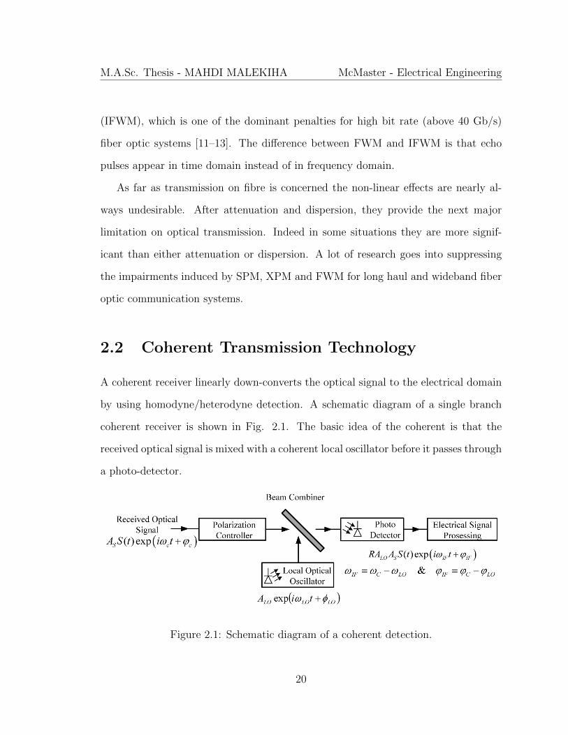
2.2 Coherent Transmission Technology
A coherent receiver linearly down-converts the optical signal to the electrical domain
by using homodyne/heterodyne detection. A schematic diagram of a single branch
coherent receiver is shown in Fig. 2.1. The basic idea of the coherent is that the
received optical signal is mixed with a coherent local oscillator before it passes through
a photo-detector.
Figure 2.1: Schematic diagram of a coherent detection.
20

M.A.Sc. Thesis - MAHDI MALEKIHA McMaster - Electrical Engineering
Suppose that the polarization of the received signal is perfectly aligned with that
of the local oscillator (LO). The state of polarization of the received signal can be
controlled using the polarization controller (PC). Let the transmitted signal be
ET (t) = A0s(t) exp(iωct) (2.19)
Let us assume a perfect optical channel that introduces neither distortion nor noise.
Only the phase of the optical carrier is changed due to propagation. Let the received
signal after the PC be
ER(t) = Ass(t) exp[i(ωct+ φc)] (2.20)
where Ass(t) is the complex received field envelope, ωc is the optical carrier and φ is
the phase. The electrical field of local oscillator is given by
ELO(t) = ALO exp[i(ωLOt+ φLO)] (2.21)
These two signals are combined using a optical beam combiner and pass through a
photo-detector (PD). The output electrical current of the PD is proportional to the
absolute square of the incident optical field, and it can be written as
I(t) = R
∣∣∣∣qS(t)√2
+qLO(t)√
2
∣∣∣∣2 =R
2|Ass(t)|2 + |ALO|2 + 2AsALORes(t)exp[i(ωIF t+ φc − φLO)]
(2.22)
where
ωIF = ωc − ωLO (2.23)
is called the intermediate frequency. Typically, the LO output power, A2LO, is much
21

M.A.Sc. Thesis - MAHDI MALEKIHA McMaster - Electrical Engineering
larger than the signal power, A2s, and therefore, the first term in Eq. (2.22) can be
ignored. Since the LO output is continues wave, A2LO is a constant and it leads to a
DC component in the photo current, which can be removed by capacitive coupling.
Therefore, the signal that goes to the front-end can be written as
Id(t) = RAsALORes(t)exp[i(ωIF t+ φc − φLO)] (2.24)
If ωIF = 0, such a receiver is known as homodyne receiver. Otherwise, it is called
heterodyne receiver. For homodyne receiver, the phase of the received carrier φc
should be exactly the same as the phase of the local oscillator φLO. This can be
achieved using optical phase locked loop, or it can be post-corrected using the digital
phase estimation techniques. When the phases are exactly aligned (φc = φLO), Eq.
(2.24) can be written as
Id(t) = I0Re[s(t)] (2.25)
where I0 = RAsALO. If the transmitted signal is real such as that corresponding to
the amplitude modulated signal, the real part of s(t) has all the information that
is transmitted. If the transmitted signal is complex such as that corresponding to
multilevel phase shift keying (MPSK) and quadrature amplitude modulation (QAM),
phase diversity receivers are required to fully restore the transmitted information. The
received signal and LO outputs are divided into two parts using power splitter (PS),
and they are mixed together similar to what is done before. To recover the real part
of s(t), LO phase should be aligned with the optical carrier. Similarly, to recover
the imaginary part of s(t), the LO phase should be shifted by π/2, (exp(iπ/2) = i)
with respect to optical carrier. Fig. 2.2 shows the block diagram of the single-branch
22

M.A.Sc. Thesis - MAHDI MALEKIHA McMaster - Electrical Engineering
in-phase/quadrature coherent receiver, and as can be seen the phase information of
optical carrier could be preserved using coherent detection.
Figure 2.2: Schematic diagram of the single-branch in-phase/quadrature coherent
receiver
For homo dyne detection, If the phase of the local oscillator is not fully aligned
with the phase of the carrier, Eq. (2.24) can be written as
Id(t) = I0Re[s(t) exp(i∆φ)], (2.26)
where ∆φ = φc − φLO is the phase error. If ∆φ is π/2 and s(t) is real, Id(t) = 0,
and therefore, the phase error leads to bit error. In contrast in heterodyne detection
when, when local oscillator frequency ωLO = 0 is deviating from the received optical
23

M.A.Sc. Thesis - MAHDI MALEKIHA McMaster - Electrical Engineering
carrier frequency ωc = 0. The optical signal first converted in to the microwave
domain. Typically intermediate frequency is in the microwave or radio wave range
and the resulting signal can be interpreted as the message s(t) being modulated by
the microwave or radio carrier of frequency ωIF . It is because the microwave LO
phase could be achieved using electrical phased locked loop (PLL), and therefore
the optical PLL is no longer needed in heterodyne detection. However, this merit is
gained at the cost of 3-dB penalty in the receiver sensitivity compared to homodyne
detection. Recently, with the advent of high speed digital signal processors (DSPs),
phase estimation can be done in digital domain for homodyne/heterodyne receivers,
and therefore, analog PLL is no longer required. ,Advantage of homodyne detection
is the optical receiver bandwidth (and also speed of A/D converter) is of order of
symbol rate, Bs. In contrast for heterodyne detection, the receiver bandwidth should
be ∼ 2Bs centered around ωIF .
Since the coherent detection is linear in nature, the complex-valued electrical field
with phase information can be achieved, and therefore, the amplitude, phase and
frequency of the optical carrier can all be utilized to carry the information. There
are several advantage for a coherent detection over a direct detection. First, the
receiver sensitivity can be greatly improved by making the power of local oscillator
sufficiently large. Second, the availability of higher-order modulation schemes in a
coherent optical communication can further improve the spectral efficiency compared
to conventional intensity modulation direct detection systems. Third, the heterodyne
detection allow closely spaced WDM channels compared to that of direct detection
systems. Last, the linearly detected signal by coherent detection enables the post
signal processing in the electrical domain. Therefore, the electronic compensation
24

M.A.Sc. Thesis - MAHDI MALEKIHA McMaster - Electrical Engineering
of chromatic dispersion (CD), polarization mode dispersion (PMD), and the fiber
nonlinearity can be performed after the coherent detection using advanced DSP tech-
niques. The combination of coherent detection and DSP is expected to become a
very important transmission technique for the next generation of fiber optic commu-
nication systems due to its potential capacity and flexibility with various pre- and
post-signal processing schemes in the electrical domain [14–22].
2.3 Dispersion Compensation Techniques
In fiber optic communication systems, information is transmitted over an optical fiber
by using a coded sequence of optical pulses, whose width is set by the bit rate B of the
system. Dispersion-induced broadening of pulses is undesirable as it interferes with
the detection process, and it leads to errors if the pulse spreads outside its allocated
bit slot (TB = 1/B). Clearly, group velocity dispersion (GVD) limits the bit rate B
for a fixed transmission distance L. The dispersion problem becomes quite serious
when optical amplifiers are used to compensate for fiber losses because L can exceed
thousands of kilometers for long-haul systems. The implementation of fiber dispersion
compensation can be done at the transmitter, at the receiver or within the fiber link.
In this section, several dispersion compensation techniques are discussed, and their
advantage and disadvantage are also compared.
Before the development of high-speed powerful DSPs, conventional optical sys-
tems employ a dispersion management scheme that places a dispersion compensation
module (DCM) at the amplifier site to negate the dispersion of the transmission link.
The DCM compensates GVD while the amplifier takes care of fiber losses. A DCM
25

M.A.Sc. Thesis - MAHDI MALEKIHA McMaster - Electrical Engineering
could be a dispersion compensating fiber (DCF) with the reverse sign of GVD pa-
rameters as that of the transmission fiber, or an optical filter with inverse transfer
function of the fiber channel.
The use of DCF for dispersion compensation was first proposed in 1980, but due
to the high loss of DCFs, this technique was not applied in practice until 1990s when
the erbium-doped fiber amplifier (EDFA) was presented. A typical transmission fiber
(TF) consisted of the standard single mode fiber (SSMF) with anomalous dispersion
at 1550 nm and the DCF placed at the optical amplifier site within a double stage
amplifier and it is shown in Fig 2.3.
Figure 2.3: A transmission span with a DCF. β21, L1 and β22, L2 are the GVD
parameter and length for SSMF and DCF, respectively
It can be shown that the total transfer function of SSMF cascades with a DCF is
given by
Hspan(ω) = exp
[jω2
2(β21L1 + β22L2)s(t)
](2.27)
It is evident from Eq. (2.27), that the perfect dispersion compensation is realized if
β21L1 + β22L2 = 0. (2.28)
Therefore, the optical pulses at the receiver are not broadened, and there is no ISI due
26

M.A.Sc. Thesis - MAHDI MALEKIHA McMaster - Electrical Engineering
to dispersion. Since β21 is negative (anomalous GVD) for standard fibers, therefore
DCF must have normal dispersion β22 > 0, such that the accumulated dispersion
in Eq. (2.28) becomes zero. The DCF with large positive value of GVD have been
developed for the sole purpose of dispersion compensation in order to keep L2 as
small as possible. The use of DCFs provides an all-optical technique that is capable
of overcoming the detrimental effects of chromatic dispersion (CD) in optical fibers,
provided the average signal power is low enough that the nonlinear effects remain
negligible.
This scheme is quite attractive but suffers from two problems. First, insertion
losses of a DCF module typically exceed 5 dB. Insertion losses can be compensated
by increasing the amplifier gain but only at the expense of enhanced amplified spon-
taneous emission (ASE) noise. Second, because of a relatively small mode diameter
of DCFs, the effective mode area is only ∼ 20 µm2 . As the optical intensity is large
inside a DCF at a given input power, the nonlinear effects are considerably enhanced
[23]. These two shortage limits the use of DCF in the long-haul fiber links.
Since the early 1990s, there has been great interest in using electronic equalizers as
replacements for optical dispersion compensating modules at the receiver. Compared
with the optical counterpart, the electronic dispersion compensation (EDC) has the
advantages of lower cost and ease of adaption.
For a transmitter based dispersion compensation scheme, fiber dispersion can be
canceled by pre-distorting the input pulses before they are launched in to the fiber
link. Koch and Alferness presented a technique in 1985 to compensate fiber dispersion
using the synthesis of pre-distorted signal [21]. The pre-chirped Gaussian pulse were
obtained using a frequency modulated (FM) optical carrier as input to an external
27
M.A.Sc. Thesis - MAHDI MALEKIHA McMaster - Electrical Engineering
modulator for amplitude modulation (AM). The output pulse is a chirped Gaussian
pulse with the chirp parameter C > 0 such that Cβ2 < 0 in a single mode optical
fiber with typical β2 = −21 ps2/Km. The dispersion induced chirp is canceled out the
intentionally induced chirp in the input pulses, and therefor, the pulse broadening is
suppressed at the output of fiber. An alternative to implement signal pre-distortion
is making use of DSP. With the advances in the performance of high-speed devices
since 1990s, the signal pre-distortion can be done in electrical domain using DSP for
the bit rate of 10 Gb/s and above in fiber optical transmission systems.
The disadvantage of pre-compensating scheme is that the exact dispersion com-
pensation can not be achieved without the knowledge of the transmission fiber link.
Furthermore, even if the transfer function of the fiber link is fully known, the op-
timum performance of the dispersion compensation is still hard to reach because in
fiber link when an optical pulse propagate, other linear and nonlinear effects such as
polarization mode dispersion and self phase modulation, interact with dispersion and
change the pulse shape further and leading to lower performance of pre-compensation
schemes. To avoid prior-knowledge of the fiber link setup requirement and achieve
the optimum dispersion compensation, the dispersion compensation moved from the
transmitter to the receiver and this schemes called dispersion post compensation or
receiver based dispersion compensation.
There are several receiver-based EDC techniques. A linear equalizer can be used
between the receiver and the detector to compensate for the ISI caused by fiber dis-
persion. A transversal filter (tapped delay line) is often used as a linear equalizer, and
the weight coefficients can be adaptively adjust using well known least-mean square
28

M.A.Sc. Thesis - MAHDI MALEKIHA McMaster - Electrical Engineering
(LMS) and zero-forcing (ZF) algorithms. For a conventional fiber optic communi-
cation system with direct detection, due to the power-law detection the linear EDC
techniques discussed above can only partially undo the fiber dispersion because linear
dispersion-induced distortion in optical domain becomes nonlinear in the electrical
domain. Some nonlinear equalization techniques were therefore developed for direct
detection.
For a fiber optic communication system with direct detection, the nonlinearity in-
duced by power law of the photo-detector make the dispersion compensation scheme
more complex and less efficient. With development of powerful digital signal proces-
sors (DSPs) during the 2000s, the difficulty in tracking the received optical carrier
phase in an optical coherent receiver was overcomed by using digital carrier phase
estimation circuit [24]. Hence, the coherent receiver combined with electronic disper-
sion compensation (EDC) using DSP has become more practical in past decade. Since
the phase information of transmitted signal is preserved in the coherent systems, in
the other words the complex valued electrical field is fully detected at the coherent
receivers, more options are available in coherent optical systems compare to direct
detection.
One of the most attractive advantage of the receiver-based EDC is that the fiber
dispersion can be adaptively compensated either in frequency-domain or time-domain
even without the knowledge of the transmission link, since the impairment introduced
by power-law detection is absent in coherent receivers. With the rapidly increasing
demand for the bandwidth, the fiber optic communication tends to transmit high
bit-rate information data through multi-carriers and WDM systems and this will
suffer from the distortion caused by higher-order dispersion effects due to its large
29

M.A.Sc. Thesis - MAHDI MALEKIHA McMaster - Electrical Engineering
bandwidth. Therefore, the compensation of higher-order dispersion effects become
more and more important in long-haul high-speed fiber-optic communication systems
and it seems that receiver-based EDC going to be main dispersion compensation
technique of future.
2.4 Backward Propagation
In high-speed wavelength division multiplexed (WDM) systems, the interaction of
fiber nonlinearity and dispersion leads to many degrading effects, limiting the total
capacity as well as the achievable transmission distance. Digital backward propaga-
tion (DBP) schemes have drawn significant research interest recently because of their
ability to undo fiber linear and nonlinear impairments. Electronic backward propa-
gation was first studied in 2007 by Killey et al. as a transmitter-based compensation
method [19]. Since in the absence of coherent detection, manipulation of the field is
only possible at the modulator. However, with the coherent detection, recovery of the
received electric field enables receiver-based backward propagation, which was first
studied in 2008 [25]. Receiver-based backward propagation has the advantage that it
can ultimately be adaptive without the need for a feedback channel. The basic idea
behind backward propagation (BP) can be understood from the governing equation
of fiber propagation. The propagation of the electrical field envelope of an optical
signal can be modeled by a scalar nonlinear Schrdinger equation (NLSE) in optical
fiber [9]
∂u
∂z=[D + N
]u, (2.29)
30

M.A.Sc. Thesis - MAHDI MALEKIHA McMaster - Electrical Engineering
where D denotes the linear operator given by
D = −iβ2(z)
2
∂2
∂t2+β3(z)
6
∂3
∂t3− α(z)
2(2.30)
and N is the nonlinear operator given by
N = iγ(z)|u|2, (2.31)
where β2(z), β3(z), α(z) and γ(z) are the profile of second-order and third-order
dispersion coefficients, loss/gain and nonlinear coefficient, respectively. The NLSE is
an invertible equation in absence of noise, and the transmitted signal can be exactly
recovered by backpropagating the received signal through the inverse NLSE. If the
sign of z reversed in Eq. (2.29) and the received signal is taken as the input signal,
Eq. (2.29) can be written as
∂u
∂z=[−D − N
]u, (2.32)
which is equivalent to passing the received signal through a fictitious fiber having
opposite-signed loss/gain, dispersion and nonlinearity coefficients. Therefore, the
transmitted signal can be exactly recovered using this method. This technique is
referred as backward propagation. Eq. (2.32) can be numerically solved using split-
step Fourier method (SSFM) in DSP. The performance of this scheme is limited by
noise and step size used in SSFM for backward propagation. In principle, in the ab-
sence of noise, BP can completely compensate both fiber dispersion and nonlinearity
when the step size used to solve Eq. (2.32) is chosen small enough. However, when
31

M.A.Sc. Thesis - MAHDI MALEKIHA McMaster - Electrical Engineering
the noise is present, the transmitted signal can not be completely recovered using
backward propagation because BP-based schemes can not compensate for stochastic
nonlinear impairments such as nonlinear phase noise. In fiber optic communication
systems inline optical amplifiers change the amplitude of the optical field envelope
randomly and fiber nonlinear effects such as self-phase modulation convert the am-
plitude fluctuations to phase fluctuations which is known as nonlinear phase noise.
The computational cost in digital BP increase as the step size decreases, as a result,
in practice the step size should be chosen large enough to make computational ef-
fort at transmitter/receiver affordable. BP has the advantage that it can be used
to compensate for any higher order dispersion. BP also can be implemented digi-
tally, either at transmitter/receiver or jointly at both. since backward propagation
operates directly on the complex-valued field u(z, t), this technique is universal, as
the transmitted signal can have any modulation format or pulse shape, including
multicarrier transmission using orthogonal frequency-division multiplexing (OFDM)
with quadrature amplitude modulation (QAM). The compensation of fiber nonlin-
earity and dispersion using BP has been demonstrated to enable larger launch power
and longer transmission distance in any fiber optic communication system. For this
reason, a novel backward propagation technique using highly nonlinear fibers was
proposed in this thesis for jointly compensation of fiber nonlinearity and linear effects
in optical domain.
32

Chapter 3
Analysis of Nonlinear Phase Noise
in Fiber-Optic Communication
Systems
3.1 Introduction
The response of all dielectric materials to light becomes nonlinear under strong op-
tical intensity and optical fiber has no exception. Due to the fiber Kerr effect, the
refractive index of optical fiber increases with optical intensity, inducing intensity
dependent nonlinear phase shift. The spontaneous emission of light is a phenomena
which appears during the optical signal amplification. It is not correlated with signal
and has an additive nature. In long-haul lightwave systems with lumped amplifiers
placed periodically along the link, each amplifier adds noise caused by the amplified
spontaneous emission (ASE) that propagates with the signal in multiple fiber sections.
The nonlinear term in the NLS equation couples the ASE and signal, and therefore,
33

M.A.Sc. Thesis - MAHDI MALEKIHA McMaster - Electrical Engineering
modifies the signal through the three nonlinear effects, self phase modulation (SPM),
cross phase modulation (XPM) and four wave mixing (FWM).
Gordon and Mollenauer (1990) first showed that when optical amplifiers are used
to periodically compensate for fiber loss, nonlinear phase noise is induced by the in-
teraction of the fiber Kerr effect and optical amplifier noise, often called the Gordon-
Mollenauer effect [26]. Here, nonlinear phase noise is induced by self phase modulation
through the amplifier noise in the same polarization as the signal and within an op-
tical bandwidth matched to the signal. Phase modulated optical signals, both phase
shift keying (PSK) and differential phase shift keying (DPSK), carry information by
the phase of an optical carrier. Added directly to the phase of a signal, nonlinear
phase noise degrades both PSK and DPSK signals and limits the maximum transmis-
sion distance. Early literatures studied the spectral broadening induced by nonlinear
phase noise [27–29]. The performance degradation due to nonlinear phase noise is
assumed the same effect as that due to laser phase noise. However, the statistical
properties of nonlinear phase noise are not the same as laser phase noise. The prob-
ability density function (PDF) of nonlinear phase noise is required for performance
evaluation of a phase modulated signal with nonlinear phase noise. However, because
of fiber nonlinearity, it is usually hard to obtain the exact expression for PDF of
nonlinear phase noise but if the actual PDF is approximated by a Gaussian one can
use variance in order to evaluate system performance. When the optical signal is
periodically amplified by optical amplifiers, amplifier noise is unavoidably added to
the optical signal. In long-haul optical communication systems, nonlinear phase noise
is accumulated span after span and the accumulation of nonlinear phase noise is the
summation of the contribution from each individual span. As a result the system
34

M.A.Sc. Thesis - MAHDI MALEKIHA McMaster - Electrical Engineering
performance is dominated by nonlinear phase noise, rather than thermal and laser
phase noise.
In addition to nonlinear phase noise, amplifier ASE noise also affects optical pulses
and induces not only energy and phase fluctuations but also timing jitter by shifting
each pulse in a random fashion from its original location within the bit slot. The
physical origin of ASE-induced time jitter can be understood by noting that optical
amplifiers affect not only the amplitude but also the phase of the amplified signal.
Time-dependent variations in the optical phase shift the signal frequency from the
carrier frequency by a small amount after each amplifier. Since the group velocity of
an optical pulse depends on its carrier frequency, because of dispersion, the speed at
which a pulse propagates through the fiber is affected by each amplifier in a random
fashion. Such speed changes produce random shifts in the pulse position at the
receiver and are responsible for the ASE-induced timing jitter.
In this chapter, we derive an analytical expression for electric field and variance
of nonlinear phase noise in dispersion-managed coherent fiber optic system based on
binary PSK using a perturbation theory. At the end of the chapter we validate our
analytical results and show that the results are in good agreement with numerical
simulation. We are also suggesting that our analytical expression for variance of
nonlinear phase noise could be used as a design tool to optimize the various parameters
such as launch power or pre- and post-dispersion compensation percentage of the
coherent optical system.
35
M.A.Sc. Thesis - MAHDI MALEKIHA McMaster - Electrical Engineering
3.2 Quasi-Linear Systems
In many occasions fiber link can be seen as a quasi-linear system, if transmitted
power is well controlled such that the nonlinear effect of fiber is not too large. Our
work is based on this assumption and the nonlinearity of a fiber can be described
by first-order and second-order perturbation approximation. In quasi-linear systems,
dispersive effects are much stronger than the nonlinear effects, and therefore, the fiber
nonlinearity can be considered as a small perturbation on the linear system. Since
the dispersive effects are dominant in quasi-linear systems, neighboring pulses overlap
and this system is also known as strongly pulse overlapped system [13] or pseudo-
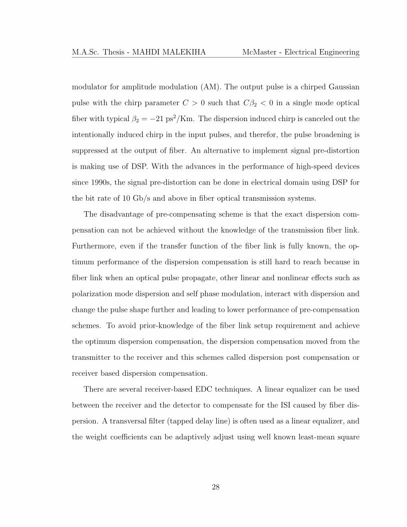
linear system [30]. Fig. 3.1 shows the typical coherent fiber-optic transmission system
based on binary PSK.
Figure 3.1: Schematic diagram of a coherent fiber optic system.
The optical field envelope in a fiber-optic transmission system can be described
by the nonlinear Schrodinger equation (NLSE),
i∂u
∂z− β2(z)
2
∂2u
∂t2− iα
2u = −γ|u|2u+ iR(z, t) (3.1)
36

M.A.Sc. Thesis - MAHDI MALEKIHA McMaster - Electrical Engineering
where α(z) is the loss/gain profile which includes fiber loss as well as amplifier gain,
β(z) is the second-order dispersion profile and γ is the fiber nonlinear coefficient.
R(z, t) represents the noise field due to amplification, i.e.,
R(z, t) =Na∑m=1
δ(z − Lm)n(m)(t), (3.2)
where Lm is the location of an amplifier, Na is the number of amplifiers, and n(m)(t)
is the noise field due to an amplifier located at Lm. The mean and autocorrelation
function of the noise field are given by
〈n(m)(t)〉 = 0, (3.3)
〈n(m)(t)n(m)∗(t′)〉 = ρmδ(t− t′) (3.4)
and
〈n(m)(t)n(m)(t′)〉 = 0, (3.5)
where ρm is the amplified spontaneous emission (ASE) power spectral density (PSD)
per polarization of an amplifier located at Lm The spectral density of spontaneous
emission-induced noise is nearly constant (white noise) and can be written as [26]
ρm = nsphν(Gm − 1), (3.6)
where Gm is the gain of the amplifier, h is Planck’s constant and, v is the mean optical
carrier frequency. The parameter nsp is called the spontaneous-emission factor (or the
37

M.A.Sc. Thesis - MAHDI MALEKIHA McMaster - Electrical Engineering
population-inversion factor) and is given by
nsp =N2
N2 −N1
(3.7)
where Nl and N2 are the atomic populations for the ground and excited states, re-
spectively. We assume that the amplifier compensates for the fiber loss. To separate
the fast variation of optical power due to fiber loss/gain, we use the following trans-
formation [31],
q = α(z)u, (3.8)
and
∂q
∂z=∂a
∂zu+ a
∂u
∂z, (3.9)
if
∂a
∂z= −α(z)
2a. (3.10)
Substituting Eqs. (3.9) and (3.10) in Eq. (3.1), we obtain
i∂u
∂z− β2(z)
2
∂2u
∂t2= −γa2(z) |u|2 u+ iR(z, t). (3.11)
Solving Eq. (3.9), we find
a(z) = exp
[−∫ z
0
α(s)
2ds
]. (3.12)
Between amplifiers, when the fiber loss is constant and Eq. (3.12) becomes
a(z) = exp (−αz/2) . (3.13)
38

M.A.Sc. Thesis - MAHDI MALEKIHA McMaster - Electrical Engineering
Note that the mean optical power fluctuates due to fiber loss and amplifier gain,
but < |U(z)|2 > is independent of distance since the variations due to loss/gain is
represented by a(z). Fig. 3.2 shows the typical dispersion and loss/gain profiles of
a long-haul dispersion-managed fiber optic system. Eq. (3.11) can be solved using
perturbation theory.
Figure 3.2: Typical dispersion and loss/gain profiles of a long-haul dispersion-
managed fiber-optic system. Pre- and post- compensation are not shown.
39

M.A.Sc. Thesis - MAHDI MALEKIHA McMaster - Electrical Engineering
The solution of Eq. (3.11) can be written as
u(t, z) = u0(t, z) + γu1(t, z) + γ2u2(t, z) + · · · , (3.14)
where uj(t, z) is the j-th order solution. Using Eq. (3.14), we find
|u(t, z)|2u(t, z) =
∣∣∣∣∣∞∑n=0
γnun
∣∣∣∣∣2 ∞∑n=0
γnun. (3.15)
submitting Eq. (3.15) in Eq. (3.11) and separating terms proportional to γn, n =
0, 1, 2, . . . , we obtain
(γ0) : i∂u0∂z− β2
2
∂2u0∂t2
= 0, (3.16)
(γ1) : i∂u1∂z− β2
2
∂2u1∂t2
= −a2(z) |u0|2 u0, (3.17)
(γ2) : i∂u2∂z− β2
2
∂2u2∂t2
= −a2(z)(2 |u0|2 u1 + u20u
∗1
). (3.18)
Eq. (3.16) is the linear Schrodinger equation. Eqs. (3.17) and (3.18) represent the
first- and second-order corrections to the linear solution due to the nonlinear effects.
When nonlinear effects are small, the terms of the order γn, n > 2, can be ignored.
Eq. (3.16) can be solved using the Fourier transform technique. The solution is
u0(t, z) = F−1u0(ω, 0) exp
[iω2S(z)/2
], (3.19)
where u0(ω, 0) = F [u0(t, 0)], u0(t, 0) = u(t, 0) and S(z) is the accumulated dispersion
S(z) =
∫ z
0
β2(x)dx. (3.20)
40

M.A.Sc. Thesis - MAHDI MALEKIHA McMaster - Electrical Engineering
Eqs. (3.17) and (3.18) can also be solved using the same technique. Typically, in
pseudo-linear systems, the nonlinear effects are smaller than dispersive effects and
first order correction u1(t, z) is often adequate to describe the nonlinear propagation.
However, when the transmission distance is long and/or launch power is large, second
order perturbation theory is needed [32]. Therefore, in the next section, we derive
an analytical expression for electric field and variance of nonlinear phase noise in
dispersion-managed coherent fiber optic system based using a second-order perturba-
tion theory.
3.3 Mathematical Derivation of Nonlinear Phase
Noise Variance
In this section, we derive the variance of nonlinear phase noise for the received phase
shift keying signals in a coherent fiber optic system. In the absence of nonlinear effects
and amplifier noise, if a Gaussian pulse is launched to the fiber, its propagation is
given by Eq. (3.19)
u0(z, t) = ulin(z, t) =√EF (z, t), (3.21)
and
F (z, t) =
[p(z)√π
]1/2exp
− [p2(z) + iC(z)]t2
2+ iθ0(z)
(3.22)
This appendix A.1 provides details of the calculation and E is pulse energy, p(z),
C(z) and θ0(z) are the inverse pulse width, chirp and phase factor, respectively, and
41

M.A.Sc. Thesis - MAHDI MALEKIHA McMaster - Electrical Engineering
they are given by
p(z) =T0√
T 40 + S2(z)
, C(z) =S(z)p2(z)
T 20
(3.23)
θ0(Z) =1
2tan−1[
S(z)
T 20
]. (3.24)
Here, T0 is the half-width at 1/e intensity point, and S(z) is the accumulated disper-
sion given by Eq. (3.20). The peak power, P and energy, E are related by
P =E
Teff(3.25)
where Teff =√πT0, and F (z, t) is normalized such that
∫ +∞
−∞|F (z, t)|2dt = 1 (3.26)
Solving Eqs. (3.17) and (3.20) using the Fourier transform technique for a single
Gaussian pulse, the first-order and second-order nonlinear correction terms can be
found as
u1(z, t) = γ|E|√Eg(1)(z, t)F (z, t), (3.27)
and
u2(z, t) = γ2|E|2√Eg(2)(z, t)F (z, t), (3.28)
where g(1)(z, t) and g(2)(z, t) can be found as
g(1)(z, t) = jT 20√π
∫ z
0
exp(−a(s)−∆(s)t2)
T1(s)|T 21 (s)|
√δ(z, s)R(s)
ds (3.29)
42
M.A.Sc. Thesis - MAHDI MALEKIHA McMaster - Electrical Engineering
and
g(2)(z, t) = −2g(2)x (z, t) + g(2)y (z, t) (3.30)
where
g(2)x (z, t) =T 30
π
∫ z
0
∫ s
0
exp(−a(s+ s′)−∆x(s)t2)
T1(s′)|T 21 (s′)||T 2
1 (s)|√δ(s, s′)R(s′)
× dsds′√δx(s, s′, z)Rx(s, s′)
(3.31)
and
g(2)y (z, t) =T 30
π
∫ z
0
∫ s
0
exp(−a(s+ s′)−∆x(s)t2)
T ∗1 (s′)|T 21 (s′)|T 2
1 (s)√δ∗(s, s′)R∗(s′)
× dsds′√δy(s, s′, z)Ry(s, s′)
(3.32)
where T 21 = T 2
0 −iS(z) and ∆(s) , ∆k(s, s′, z) k = x, y, δ(z, s), etc are given by Kumar
et. al. [32] (Appendix A.2), where a second-order perturbation theory was developed
for self phase modulation (SPM).
Now, consider the optical field envelope immediately after an amplifier located at
Lm. The optical field envelope in the absence of amplifier noise can be written as
u(Lm, t) =√E
+∞∑j=0
γj|E|jg(j)(Lm, t)F (Lm, t). (3.33)
In this section, we study the combined effect of SPM and amplifier noise using the
second-order perturbation theory. For the analytical treatment of the problem, we
approximate the field given by Eq. (3.33) with best-fitting Gaussian pulse, which is
in the form of
u(Lm, t) '√EmF (Lm, t), (3.34)
43

M.A.Sc. Thesis - MAHDI MALEKIHA McMaster - Electrical Engineering
where √Em =
∫ +∞
−∞u(Lm, t)F
∗(Lm, t)dt. (3.35)
Here√Em is a complex electrical field amplitude which takes into account the first-
order and second-order nonlinear effects.
Focusing only on the impact of the noise added by this amplifier, the optical field
envelope at Lm+ can be written as
u(Lm+, t) =√EmF (Lm, t) + n(t), (3.36)
where n(t) ≡ n(m)(t) is the noise field added by the amplifier at Lm. In this section,
we consider only two noise modes given by
n(t) = (n0r + in0i)F (Lm, t) (3.37)
where n0r = Ren0, and n0i = Imn0 are the amplitudes of the in-phase and
quadrature components of the noise field added by the amplifier at Lm, respectively,
and n0 is the complex amplitude of the noise field. The analysis of nonlinear phase
noise with higher order noise modes (arbitrary DOF) have been carried out in Ref.
[33], and the result show that the impact of higher order noise is negligible for dis-
tances of practical interest. Substituting Eq. (3.37) in Eq. (3.36), we find
u(Lm+, t) = (√Em + n0)F (Lm, t) (3.38)
Thus, the complex amplitude of the field envelope has changed because of the amplifier
noise. Treating Eq. (3.38) as the initial condition, the zeroth-order (i.e. linear) optical
44
M.A.Sc. Thesis - MAHDI MALEKIHA McMaster - Electrical Engineering
field envelope is described by
u(0)(z, t) = (√Em + n0)F (z, t), z > Lm (3.39)
In practical systems operating in the pseudo-linear regime, the dispersion of the trans-
mission fibers is fully compensated at the receiver either in optical or electrical do-
main. i.e. S(Ltot) = 0, and therefore, F (Ltot, t) = F (0, t). Solving Eqs. (3.17)
and (3.18) with the zeroth order solution given by Eq. (3.39) and the condition
S(Ltot) = 0, the total field envelope at the end of the transmission line is
u(Ltot, t) = (√Em + n0)×
+∞∑j=0
γj|√Em + n0|2jg(j)(Ltot, t)F (Ltot, t)
= (√Em + n0)×
+∞∑j=0
γj|√Em + n0|2jg(j)(Ltot, t)F (0, t)
(3.40)
where g(0)(z, t) = 1, and g(j)(z, t), j = 1, 2 are given by Eqs. (3.29) and (3.30).
The output of in-phase-quadrature (IQ) coherent receiver has two output currents
which are proportional to real and imaginary parts of the optical field envelope. For
simplicity, we assume that the constant of proportionality to be unity, since it does
not affect the performance of a long-haul fiber-optic system. The output of the IQ
receiver passes through the digital signal processing (DSP) unit after A/D converter
and arbitrary filter shapes can be realized using DSP. We assume that the output of
the IQ receiver passes through a matched filter, or equivalently a correlator and the
45
M.A.Sc. Thesis - MAHDI MALEKIHA McMaster - Electrical Engineering
decision is based on the correlator output
uf =
∫ +Ts2
−Ts2
u(Ltot, t)F∗(0, t)dt
'+∞∫−∞
u(Ltot, t)F∗(0, t)dt
(3.41)
where Ts is the symbol interval. Substituting Eq. (3.40) in Eq. (3.41) and keeping
the terms up to second-order in γ, we find
uf = (√Em + n0)
+2∑j=0
γj|√Em + n0|2jg(j)f , (3.42)
where
g(j)f =
+∞∫−∞
g(j)f (Ltot, t)F
∗(0, t)dt. (3.43)
The phase of the correlator output is
φ = tan−1[ImufReuf
]= φd + δφm (3.44)
where φd is deterministic phase change due to self phase modulation in the absence of
amplified spontaneous emission (ASE), and δφm is the stochastic phase change due
to ASE of amplifier located at Lm and signal due to SPM. δφm can be divided into
three parts,
δφm = δφ(0)m + δφ(1)
m + δφ(2)m (3.45)
where δφ(0)m is the linear phase change due to ASE, δφ
(1)m and δφ
(2)m are the first- and
second-order nonlinear phase changes due to ASE and SPM interaction, respectively.
46

M.A.Sc. Thesis - MAHDI MALEKIHA McMaster - Electrical Engineering
They can be calculated as
δφ(0)m =
1√Emr
n0i +
√Emi
Emr
n0r, (3.46)
δφ(1)m = 2γ
√Emi g
(1)fr n0i + 2γ
√Emr g
(1)fr n0r (3.47)
and
δφ(2)m = 4γ2|Em|
√Emi g(2)fr − g
(1)fr g
(1)fi n0i
+ 4γ2|Em|√Emr g(2)fr − g
(1)fr g
(1)fi n0r
(3.48)
where g(j)fr (z) = Reg(j)f (z) and g
(j)fi (z) = Img(j)f (z), where j = 0, 1, 2 and n0r =
Ren0 and n0i = Imn0. In Eqs. (3.47) and (3.48), we have ignored terms pro-
portional to γ3, n20r, n
20i and n0rn0i. Variance of phase noise can be easily found by
squaring Eq. (3.45), and averaging the noise terms using Eqs. (3.3) to (3.5), we
obtain [34]
〈δφ2m〉 =
ρm2
1√Emr
+ 2γ√Emi g
(1)fr
+ 4γ2|Em|√Emr [g
(2)fr − g
(1)fr g
(1)fi ]
2
+ρm2
√Emi
Emr
+ 2γ√Emrg
(1)fr
+ 4γ2|Em|√Emr [g
(2)fr − g
(1)fr g
(1)fi ]
2
.
(3.49)
Eq. (3.45) provides variance of the phase noise that includes both first-order and
second-order nonlinear effects and derivation of this equation is the main contribution
of this chapter.
47

M.A.Sc. Thesis - MAHDI MALEKIHA McMaster - Electrical Engineering
Since the noise of amplifiers are statistically independent, variance of phase noise
due to all the amplifiers is
〈δφ2〉 =Na∑m=1
〈δφ2m〉 (3.50)
For M-ary PSK signals, symbol error probability is determined solely by the prob-
ability density function (PDF) of the phase. Under the Gaussian PDF assumption,
the variance calculated from Eq. (3.50) can be related to the symbol error probability
for BPSK signals [23, 35]. Eq. (3.50) is valid for arbitrary dispersion map when the
dispersion of the transmission fibers is fully compensated either at the transmitter,
receiver or inline (i.e. S(Ltot = 0)).
3.4 Numerical Simulations and Result
To test the accuracy of the perturbation theory, numerical simulation of the NLS
equation is carried out using the symmetric split-step Fourier scheme (SSFS) [9]. The
main idea of SSFS is to separate the linear and nonlinear part of the NLS equation.
More specifically, propagation from z to z + h is carried out in two section, in the
middle of which the nonlinearity is lumped. In the middle, the nonlinearity acts
separately while in the neighboring sections, dispersion and absorption acting alone.
Schematic illustration of symmetric SSFS is given in Fig. 3.3.
48

M.A.Sc. Thesis - MAHDI MALEKIHA McMaster - Electrical Engineering
Figure 3.3: Schematic illustration of symmetric-SSF scheme
In Section 2.4, we have seen that NLS equation can be written as
∂u
∂z=[D + N
]u, (3.51)
where
D = −iβ2(z)
2
∂2
∂t2+β3(z)
6
∂3
∂t3− α(z)
2(3.52)
N = iγ(z)|u|2 (3.53)
In SSFS, for the linear part, D, fast Fourier transform (FFT) is employed, and for the
nonlinear operator N , the ordinary differential equation can be solved analytically, if
the step size is chosen small enough such that the nonlinear term can be assumed to
be constant. Therefore, the analytical solution of Eq. (3.51) can be approximate as
u(z + h, t) = exp
(h
2D
)exp
(hN)
exp
(Dh
2
)u(z, t) (3.54)
49

M.A.Sc. Thesis - MAHDI MALEKIHA McMaster - Electrical Engineering
3.4.1 Variance of Nonlinear Phase Noise
In this section, we implement the simulation based on analytical phase noise variance
given by Eq. (3.49) and also Monte-Carlo simulation to verify the result from the
analytical formula. 8192 runs of NLS equation are carried out and the phase variance
of the decision variable is calculated in Monte-Carlo simulation. The lumped ampli-
fication is assumed throughout this chapter. The critical simulation parameters are
listed in Table 3.1.
Table 3.1: Simulation parameters.
Bit rate 40 Gb/s
Pulse width (FWHM) 7.5 ps
Pulse shape Gaussian
Peak power (P0) 2 dBm
Spontaneous-emission factor (nsp) 1
Amplifier spacing (Lspan) 80 Km
Transmission distance (Ltot) 2400 Km
Num. of NLS runs in Monte-Carlo sim. 8192
Computational bandwidth 320 GHz
We consider a dispersion-managed fiber-optic system with two segments. The first
segment is a standard anomalous dispersion fiber and this is followed by a reversed
dispersion fiber of equal length and the same absolute dispersion. The fiber loss α
and nonlinear coefficient γ for both of the fibers are 0.2 dB /Km and 2.43 W−1Km−1
, respectively. Spontaneous-emission factor nsp is equal to 1 which corresponds to a
50
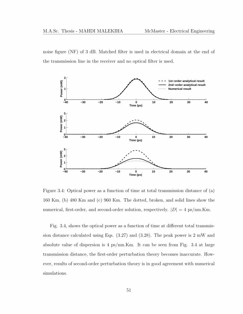
M.A.Sc. Thesis - MAHDI MALEKIHA McMaster - Electrical Engineering
noise figure (NF) of 3 dB. Matched filter is used in electrical domain at the end of
the transmission line in the receiver and no optical filter is used.
−40 −30 −20 −10 0 10 20 30 400
1
2
Time (ps)
Pow
er (
mW
)
−40 −30 −20 −10 0 10 20 30 400
1
2
3
Time (ps)
Pow
er (
mW
)
1st−order analytical result 2nd−order analytical result Numerical result
−40 −30 −20 −10 0 10 20 30 400
1
2
3
Time (ps)
Pow
er (
mW
)
Figure 3.4: Optical power as a function of time at total transmission distance of (a)
160 Km, (b) 480 Km and (c) 960 Km. The dotted, broken, and solid lines show the
numerical, first-order, and second-order solution, respectively. |D| = 4 ps/nm.Km.
Fig. 3.4, shows the optical power as a function of time at different total transmis-
sion distance calculated using Eqs. (3.27) and (3.28). The peak power is 2 mW and
absolute value of dispersion is 4 ps/nm.Km. It can be seen from Fig. 3.4 at large
transmission distance, the first-order perturbation theory becomes inaccurate. How-
ever, results of second-order perturbation theory is in good agreement with numerical
simulations.
51

M.A.Sc. Thesis - MAHDI MALEKIHA McMaster - Electrical Engineering
500 1000 1500 2000 25000
0.002
0.004
0.006
0.008
0.01
0.012
0.014
Total length (Km)
Var
ianc
e (
rad.
rad)
Numerical Result
1st−Order Analytical Result
2nd−Order Analytical Result
|D| = 4 ps/nm.Km
|D| = 10 ps/n.Km
Figure 3.5: Phase variance dependence on the total length of the transmission line.
In Fig. 3.5 the ’-’ and ’+’ marks show the phase variance calculated using the first-
and second-order analytical perturbation theory, respectively and the solid line shows
the numerical simulation results. As the dispersion increases, the variance of non-
linear phase noise due to SPM decreases consistent with the results of [36, 37]. The
nonlinear phase variance grows cubically with distance [33] and, therefore, the differ-
ence between the variances for the case of |D| = 4 ps/nm.Km and |D| = 10 ps/nm.Km
increases significantly for longer transmission lengths. In long transmission lengths,
as can be seen, there is a discrepancy between the first-order analytical results and
numerical simulation results. However, results of second-order perturbation theory is
in good agreement with numerical simulations.
52

M.A.Sc. Thesis - MAHDI MALEKIHA McMaster - Electrical Engineering
0.5 1 1.5 2 2.5 3 3.5 4 4.5 50
0.01
0.02
0.03
0.04
0.05
0.06
Peak Launch Power (mW)
Var
ianc
e (
rad.
rad)
Numerical Result
1st−Order Analytical Result
2nd−Order Analytical Result
Figure 3.6: Dependence of phase variance on peak launch power. Ltot = 2400 Km
and |D| = 10 ps/nm.Km
Fig. 3.6, shows the dependence of phase variance versus the launch power at to-
tal transmission distance of 2400 Km and |D| = 10 ps/nm.Km. When the launch
power is low, the linear phase noise dominates (because of dependence 1/E). At high
launch power, nonlinear phase noise becomes significant (because of E dependence).
At large launch powers, the first-order perturbation theory is known to become in-
accurate. However, as can be seen, results of second-order perturbation theory is in
good agreement with numerical simulations.
3.4.2 Optimizing Dispersion-Managed Fiber-Optic Systems
Fig. 3.7 shows the fiber link CONSIST of pre-, post- and inline dispersion compen-
sation.
53

M.A.Sc. Thesis - MAHDI MALEKIHA McMaster - Electrical Engineering
Figure 3.7: Dispersion-managed fiber link with pre- and post-dispersion compensa-
tion.
As we mentioned before the variance calculated using Eq. (3.50) can be related
to the symbol error probability for PSK signals and it is valid for arbitrary dispersion
maps when the dispersion of the transmission fibers is fully compensated either at
the transmitter/receiver or inline (i.e. S(Ltot) = 0). Therefore our analytical formula
can be used to optimized such systems. Fig. 3.8, shows the dependence of phase
variance on the launch power at total transmissin distance of 2400 Km and |D| =
10 ps/nm.Km using analytical and numerical methods. As can be seen in Fig. 3.8
the phase noise variance become minimum at P = 1.6 mW which corresponds to
minimum bit error rate power.
54

M.A.Sc. Thesis - MAHDI MALEKIHA McMaster - Electrical Engineering
0.5 1 1.5 2 2.5 3 3.5 40.006
0.007
0.008
0.009
0.01
0.011
0.012
0.013
0.014
0.015
Peak Launch Power (mW)
Var
ianc
e (
rad.
rad)
Numerical Result2nd−Order Analytical Result
Figure 3.8: Dependence of phase variance on peak launch power. Ltot = 2400 Km
and |D| = 10 ps/nm.Km
The numerical simulation of NLS equation is time consuming, however, the an-
alytical method based on solving NLS equation using perturbation approximation
is quite efficient and therefore the analytical variance can be obtained more easily
without requiring extensive computational efforts, and also with fairly good accuracy
for quasi-linear systems.
3.5 Conclusion
We have developed analytical expressions for the linear and nonlinear phase noise
variance due to SPM using second-order perturbation theory. It is found that as
the transmission reach and/or lunch power increase, the variance of the phase noise
calculated using first order perturbation theory becomes inaccurate. However, the
55

M.A.Sc. Thesis - MAHDI MALEKIHA McMaster - Electrical Engineering
variance calculated using second order perturbation theory is in good agreement with
numerical simulations. We have also showed that the analytical formula derived in
this chapter for the variance of nonlinear phase noise can be used as a design tool to
investigate the optimum system design parameters such as power and dispersion maps
for dispersion-managed coherent fiber optic systems based on phase shift keying.
56

Chapter 4
Optical Back Propagation for Fiber
Optic Communications Using
Highly Nonlinear Fibers
4.1 Introduction
Backward propagation (BP) schemes have drawn significant research interest recently
because of their ability to undo fiber linear and nonlinear impairments [20, 33, 38]. In
principle, BP schemes could undo the deterministic (bit-pattern dependent) nonlinear
impairments, but it can not compensate for the stochastic nonlinear impairments such
as nonlinear phase noise. Inline optical amplifiers change the amplitude of the optical
field envelope randomly and fiber nonlinear effects such as self phase modulation
(SPM) convert the amplitude fluctuations to phase fluctuations which is known as
nonlinear phase noise. The impact of nonlinear phase noise was first studied in Ref.
[26] for dispersion-free fiber-optic systems. Refs. [37] and [39] have found that the
57

M.A.Sc. Thesis - MAHDI MALEKIHA McMaster - Electrical Engineering
fiber dispersion lowers the impact of nonlinear phase noise. When the BP schemes
are used, deterministic nonlinear impairments such as self phase modulation (SPM),
cross phase modulation (XPM) and four wave mixing (FWM) can be suppressed
and therefore. stochastic nonlinear impairments such as nonlinear phase noise could
become dominant. The analysis of nonlinear phase noise is given in chapter 3 where an
analytical expressions for the linear and nonlinear phase noise variance using second-
order perturbation theory is calculated.
In this chapter, we investigate two types of backward propagation (BP) schemes.
The first scheme is the digital BP (DBP) in which the distortions due to fiber dis-
persion and nonlinear effects can be undone by solving the nonlinear Schrodinger
equation (NLSE) in digital domain with the sign of distance being reversed. The
DBP improves the transmission performance significantly. However, it requires con-
siderable amount of computational resources, and therefore, currently transmission
experiments have used DBP only in off-line signal processing. The second scheme is
optical BP (OBP) which could undo the fiber dispersion and nonlinear effects in opti-
cal domain. The OBP module is placed at the end of the fiber optic link which consists
of dispersion compensating fibers (DCF) and nonlinearity compensators (NLC). NLC
imparts a phase shift that is equal in magnitude to the nonlinear phase shift due to
fiber propagation, but opposite in sign.
In this chapter, we also introduce a novel inline optical nonlinearity compensa-
tion technique which incorporate inline optical nonlinear compensators and dispersion
compensating fibers at receiver. We will show that the in line nonlinearity compen-
sation has better performance than OBP and DBP schemes.
58

M.A.Sc. Thesis - MAHDI MALEKIHA McMaster - Electrical Engineering
4.2 Theoretical Background on Backward Propa-
gation
The signal propagation along a fiber is governed by nonlinear Schrodinger equation
(NLSE) [9] in the loss less form
∂u
∂z= −iβ2
2
∂2
∂t2+β3(z)
6
∂3
∂t3+ iγ(z)a2(z)|u|2u, (4.1)
or
∂u
∂z=[D + N
]u, (4.2)
where D and N denote the linear and nonlinear operators, receptively, which are
given by
D = −iβ22
∂2
∂t2+β3(z)
6
∂3
∂t3(4.3)
N = iγ(z)a2(z)|u|2 (4.4)
where β2, β3 and γ are the second-order and third-order dispersion coefficients and
nonlinear coefficient, respectively and
a2(z) = exp[−mod(z, Lspan)α] (4.5)
Here α is the fiber loss/gain coefficient and Lspan is the amplifier spacing (i.e. the
fiber span length between amplifiers). For simplicity, we have assumed that the
fibers in the link are identical and amplifier spacing is uniform and fiber loss is fully
compensated after each span by erbium doped fiber amplifiers (EDFAs). Eq. (4.1)
can be numerically solved using split-step Fourier method (SSFM). The solution of
59

M.A.Sc. Thesis - MAHDI MALEKIHA McMaster - Electrical Engineering
Eq. (4.1) is given by
u(t, L) = Mn(t, 0) (4.6)
where
M = exp
∫ Ltot
0
[D(z) +N(z)]dz
(4.7)
Here, Ltot is the total transmission distance. The distortions caused by dispersion
and nonlinearity, can be undone by means of digital signal processing (DSP) or an
optical back propagation module (OBM). Suppose we multiply Eq. (4.6) by M−1, we
obtain
u(t, 0) = M−1u(t, Ltot) (4.8)
Since exp(x) exp(−x) = 1 for any operator x. it follows that
M−1 = exp
−∫ Ltot
0
[D(z) +N(z)]dz
(4.9)
which is equivalent to solving the following partial differential equation
∂u
∂z= −
[D + N
]u, (4.10)
with the initial condition u(t, Ltot). Since Eq. (4.10) can be obtained by reversing the
spatial variable z in Eq. (4.1), this technique is referred to as backward propagation.
4.2.1 Digital Backward Propagation
Digital back propagation (DBP) is a technique which could undo the fiber dispersion
and nonlinear effects in electrical domain at the receiver. In DBP, fiber transmission
process is entirely reversed using fictitious fiber in digital domain with parameters (
60

M.A.Sc. Thesis - MAHDI MALEKIHA McMaster - Electrical Engineering
i.e. α, β2, β3 and γ ) with opposite sign of the transmission fiber to recover initial
signal. The amplifier with gain G is replaced by an attenuator with loss G.
Figure 4.1: Symmetric split-step Fourier method (SSFM) used to simulate the signal
forward propagation through the transmission fiber.
Typically, the NLSE is solved in electrical (digital) domain with the above param-
eters using the conventional symmetric SSFS, which is shown in Fig. 4.1. The length
of each fiber span is divided into M small segments of step size, h. Smaller h gives
better performance, but leads to more extensive calculation efforts. At the receiver,
after the coherent detection, the received signal with complex field envelope passes
through a DBP compensator implemented using DSP. An ideal DBP compensator is
shown in Fig. 4.2. In this work. we will discuss two types of DBP.
61

M.A.Sc. Thesis - MAHDI MALEKIHA McMaster - Electrical Engineering
Figure 4.2: An ideal backward propagation for a single span.
For type 1. the DBP has step size equal to amplifier spacing, called AS-DBP,
and for type 2, very small step size (same step size as that used in forward propaga-
tion) is used in BP. We call this perfect DBP. In this chapter. the NLSE is solved
using the non-iterative symmetric SSFM, and its corresponding forward propagation
mathematical expression for one fiber span is given by [9],
u(z + h, t) = exp
(h
2D
)exp
(∫ z+h
z
N(τ)dτ
)exp
(h
2D
)u(z, t) (4.11)
Note that, at the end of each span, the gain G = exp(αLspan) is applied. The
mathematical expression of backward propagation therefore can be written as
u(Ltot− (z+h), t) = exp
(−h
2D
)exp
(∫ L+(z+h)
z
N(τ)dτ
)exp
(−h
2D
)u(Ltot−z, t)
(4.12)
62

M.A.Sc. Thesis - MAHDI MALEKIHA McMaster - Electrical Engineering
where Ltot is the total transmutation distance. One of the disadvantages of the ideal
DBP is that computational complexity increases significantly as h decreases. In Ref.
[143], it is proposed to use asymmetric split-step Fourier scheme step size equal to
amplifier spacing (AS-DBP) and with a variable parameter to optimize the BER. The
AS-DBP can be realized as [40, 41],
u1(z + h, t) = u(L− z, t) exp(−iηγ|u(L− z, t)|2Leff
), (4.13)
where
u(Ltot − (z + Lspan), ω) = u(z, ω) exp
(−i[β22ω2 +
β36ω3
]Lspan
), (4.14)
Leff =1− exp(−αLspan)
α, (4.15)
α is the fiber loss coefficient, u(z, w) is the Fourier transform of ul(z, t) and η is
the variable parameter to be optimized to increase the performance. In the case of
AS-DBP. the computational complexity increases linearly with the number of spans.
4.2.2 Optical Backward Propagation
Optical back propagation (OBP) is a technique which could undo the fiber dispersion
and nonlinear effects in optical domain using optical back propagation module instead
of electrical domain [42]. The optical back propagation module consists of dispersion
compensation fibers and nonlinear compensators. A nonlinear compensator uses two
highly nonlinear fibers (HNFs) to compensate the nonlinearity of the transmission
fiber. At the end of the fiber optic link, an optical back propagation module (OBP)
63

M.A.Sc. Thesis - MAHDI MALEKIHA McMaster - Electrical Engineering
is placed as shown in Fig. 4.3a.
Figure 4.3: (a) Block diagram of a fiber-optic link with optical back propagation. (b)
Block diagram of NLC.
Let the input of OBP module be the output of fiber optic link. In order to recover
the initial field envelope at the output of OBP, the transfer function of the OBP
should be the inverse of that of the fiber-optic link M−1 given by Eq. (4.9). To
realize M−1, we utilize the symmetric split-step Fourier technique with step size of h
[9],
M−1 ≈ A(t, 0, h/2)B(t, h)A(t, h/2, 3h/2)B(t, 2h) . . . B(t, Ltot)A(t, Ltot − h/2, Ltot)
(4.16)
where
A(t, x, y) = exp(− iD(t)(y − x)
)(4.17)
64

M.A.Sc. Thesis - MAHDI MALEKIHA McMaster - Electrical Engineering
and
B(t, x) = exp
(− i∫ x
x−ha2(z)|u(t, z)|2dz
). (4.18)
Here, A(t, x, y) represents the fiber dispersive effects over the interval [x y] and B(t, x)
represents the nonlinear phase shift accumulated over a fiber length h at x. Typically,
the function a2(z) varies more rapidly than |u(t, z)|2, and therefore, in the interval
[x−h x], |u(t, z)|2 can be approximated to be independent of z, i.e. |u(t, z)|2, |u(t, x)|2
and now, the integral in Eq. (4.18) can be evaluated analytically using Eq. (4.5) as
B(t, x) = exp
(− iγheff exp[−mod(x, Lspan)α]|u(t, x)|2
)(4.19)
where
heff =m[1− exp(−αLa)]
α+
1− exp[−mod(h, Lspan)α]
α, (4.20)
with m = floor(h/Lspan). When the step size is equal to amplifier spacing, Eq. (4.19)
reduces to Eq. (4.13) i.e. AS-DBP, for simplicity we assume that the step-size is an
integral multiple of the amplifier spacing, i.e., h = mLspan , m being an integer. The
operator B takes the form
B(t, x) = exp
(−iγm[1− exp(−αLspan)]
α|u(t, x)|2
). (4.21)
The operator A can be realized using a dispersion compensating. fiber (DCF) as
shown in 4.3a. The first DCF of OBP compensates for the half of the accumulated
dispersion of the last span of the fiber optic link assuming that the step size is equal
to the amplifier spacing. The launch power to DCF is low, so that nonlinear effects
in DCF can be ignored. An amplifier is introduced to compensate for the loss in
65

M.A.Sc. Thesis - MAHDI MALEKIHA McMaster - Electrical Engineering
DCF. If there exists a fiber with negative nonlinear coefficient, the operator B can be
easily realized through self phase modulation (SPM) in such a fiber. Unfortunately,
such a fiber is not available. Here, it is proposed to realize the operator B using a
nonlinearity compensator (NLC) whose schematic is shown in Fig. 4.3b. First the
output signal of the fiber-optic link, us (= u(t, Ltot)/√
2) and a CW pump beam
(pump 1) of frequency Ω (relative to optical carrier frequency) are launched into a
highly nonlinear fiber HNLF1. The field envelope of the pump beam after propagating
a distance L1 in a dispersion-free HNLF1 is given by [9]
up1(t, L1) = up1(t, 0) exp(i2γ1Leff,1|us(t)|2 + iθ1 + iΩt
), (4.22)
where Leff,1 and γ1 are the effective length and nonlinear coefficient of HNLF1, re-
spectively and θ1 = γ1Leff,1|up1(t, 0)|2. In Eq. (4.22), the first and second terms on
the exponent represent the XPM and SPM, respectively. Lef and γ1 are so chosen
that the nonlinear phase shift due to XPM is equal in magnitude to the phase shift
given by Eq. (4.21), but of opposite sign,
γ1Leff,1 = −γm[1− exp(−αLspan)]
α. (4.23)
The signal us and the pump beam at the output of HNLF1 are multiplexed using a
WDM coupler and its output is launched into a highly nonlinear fiber HNLF2. A
second CW pump beam, pump 2 that has the same frequency as pump 1 is launched
into HNLF2. The polarization of pump 2 is chosen to. be orthogonal to signal
polarization. Typically, highly nonlinear fibers are birefringent fibers and the field
66

M.A.Sc. Thesis - MAHDI MALEKIHA McMaster - Electrical Engineering
envelope of pump 2 at the output of HNLF2 is given by [9]
up2(t, L2) = up2(t, 0) exp
(i2γ2Leff,2|us(t) + up1(t, L1)|2
3+ iθ2 + iΩt
), (4.24)
where Leff,2 and γ2 are the effective length and nonlinear coefficient of HNLF2, re-
spectively, and θ2 = γ2Leff,2|up2(t, 0)|2. As before, first and second terms on the
exponent of Eq. (4.24) represent the XPM and SPM effects, respectively. We choose
the nonlinear coefficient γ2, effective length Leff,2, powers of signal and pump 1 such
that the phase shift due to XPM in HNLF2 is quite small,
2γ2Leff,2|us(t) + up1(t, L1)|2/3 π. (4.25)
Under these conditions, Eq. (4.24) can be approximated as
up2(t, L2) ≈ up2(t, 0)
(1 +
i2γ2Leff,2|us(t) + up1(t, L1)|2
3
)exp
(i(θ2 + Ωt)
)≈ up2(t, 0) exp(iθ2)
1 + 2iγ2Leff,2(|us|2 + |up(t, 0)|2)
3exp
(iΩt)
+2iγ2Leff,2usu
?p1(t, 0)
3exp
(− i2γ1Leff,1|us(t)|2 − iθ1
)+
2iγ2Leff,2u?sup1(t, 0)
3exp
(i2γ1Leff,1|us(t)|2 + iθ1 + 2iΩt
).(4.26)
The first, second and third terms on the right hand side of Eq. (4.26) correspond to
optical signals centered around Ω, 0 and 2Ω, respectively. If we introduce an optical
band pass filter (OBF) with its center frequency at zero and bandwidth equal to the
bandwidth of us (which is much smaller than Ω), frequency components centered
67
M.A.Sc. Thesis - MAHDI MALEKIHA McMaster - Electrical Engineering
around Ω and 2Ω will be rejected by OBF. Therefore, the output of OBF is
uout = Kus(t) exp(−i2γ1Leff,1|us(t)|2
)(4.27)
where K = i2γ2Leff,2up2(t, 0)u∗p1(t, 0) exp[i(θ2 − θ1)/3] is a complex constant. Thus,
the phase shift provided by the OBP is of the form given by Eq. (4.21) which is
required for back propagation. The phase of K is a constant and it has no impact
on direct detection systems. When coherent detection is employed, this phase shift
is removed by digital signal processing (DSP) unit of the coherent receiver.
4.2.3 Inline Optical Nonlinearity Compensation Scheme
Inline optical nonlinearity compensation (IONC) is a novel technique which could
effectively undo the nonlinear effects in optical domain similar to OBP. This tech-
nique divides optical back propagation module to two parts, unlike OBP which has
both nonlinear and linear compensators at receiver, it uses optical nonlinear compen-
sators distributed throughout the fiber link before each amplifier to compensate for
each span nonlinearity and therefore, makes the system efficiently linear. Dispersion
compensation fiber (DCF) at the end of fiber link (i.e. receiver) to combat fiber
linear effect. In the next section, we will see that this scheme can outperform both
OBP and DBP techniques and gives the system longer reach and better tolerance to
nonlinearity.
68

M.A.Sc. Thesis - MAHDI MALEKIHA McMaster - Electrical Engineering
4.3 Results and Discussion
We have simulated a N−span fiber-optic transmission system without inline pre- and
post-dispersion compensation in optical domain. Table 4.1 shows the system param-
eters listed in our simulation. For perfect-BP very small step size is chosen so that
nonlinear phase does not exceed 0.0005 rad. A pseudo-random bit sequence (PRBS)
of length 262144 is used in the simulations. The symbol rate is 25 GSym/sec, mod-
ulation format = 32 quadrature amplitude modulation (QAM). We assume that the
coherent receiver is ideal and mainly focus on the impairments caused by dispersion
and nonlinearity. Backward propagation provides equalization for both linear and
nonlinear impairments, and therefore, no other equalizer is used.
Table 4.1: Simulation parameters.
Symbol rate 25 GSym/sec
Modulation format 32-QAM
Pulse shape Gaussian
Transmission fiber dispersion (β2) -21 W−1Km−1
Transmission fiber loss (α) 0.2 dB/Km
Transmission fiber nonlinear coefficient (γ) 1.1 W−1Km−1
Amplifier spacing (Lspan) 80 Km
Spontaneous-emission noise factor (nsp) 1.5
Computational bandwidth 320 GHz
69

M.A.Sc. Thesis - MAHDI MALEKIHA McMaster - Electrical Engineering
The numerical simulations of optical back propagation module and inline optical
nonlinearity compensation are carried out with the following parameters: dispersion
of DCF = -130 ps2/Km, loss of DCF = 0.4 dB/Km, nonlinear coefficient of DCF
= 4.2 W−1Km−1, nonlinear coefficient of HNLF1 fiber, γHNLF1 = 2000 W−1Km−1,
effective length of HNLF1 = 232 m, pump 1 power = 10 mW, frequency of the pump
1 (and also pump 2), n = 400 GHz, the full bandwidth of the optical band pass
filters = 87.5 GHz. When the product of effective length and nonlinear coefficient
of HNLF2 is large, the linear approximation done in Eq. (4.4.26) for XPM breaks
down leading to performance degradations. On the other hand, if the product is too
low, NLC would not compensate for transmission fiber nonlinear effects. Therefore,
we have optimized the fiber parameters of HNLF2 to obtain the best transmission
performance. The nonlinear coefficient γHNLF2 and effective length of HNLF2 are
chosen as 1000 W−1Km−1 and 200 m, respectively, and power of pump 2 = 5.625 mW.
When the step-size is equal to amplifier spacing, effective length of HNLF1 = 232 m.
When the step-size is twice the amplifier spacing, the effective length is doubled so
that the nonlinear phase shift accumulated over two spans can be compensated. It
may be possible to design the OBP module with all the NLC units sharing the same
pump.
70

M.A.Sc. Thesis - MAHDI MALEKIHA McMaster - Electrical Engineering
−8 −6 −4 −2 0 2 4 6 8
−6
−4
−2
0
2
4
T/Ts
Re[
u] (
Arb
itrar
y U
nit)
Tx outputwith DCF, w/o NLC1−span OBP
Figure 4.4: Optical field envelope vs normalized time. Ts = symbol interval, trans-
mission distance = 800 Km, peak launch power to fiber-link = 0 dBm and nsp =
0.
Fig. 4.4 shows the real part of the optical field envelope for different cases. The
amplifier noise is turned off to see clearly the distortions due to fiber nonlinear effects.
The solid and broken lines show the field envelopes at the transmitter output and
OBP output, respectively. The dotted line shows the field envelope at the receiver
with DCF and without NLC. As can be seen, the field envelope with OBP is closer
to the transmitter output than that in the case, with DCF and without NLC.
71

M.A.Sc. Thesis - MAHDI MALEKIHA McMaster - Electrical Engineering
−4 −3 −2 −1 0 1 210
−4
10−3
10−2
10−1
100
↑ FEC limit, 2.1 × 10⁻³
Average launch power (dBm)
BE
R
2−span OBP1−span OBPDBP − 4 Sam/SymDispersion compensation only
Figure 4.5: Bit error rate vs average launch power to the fiber-optic link. Transmission
distance = 800 Km.
Fig. 4.5 shows the bit error rate (BER) as a function of transmission fiber launch
power. Solid lines show the cases of optical backward propagation with step-size equal
to Lspan (1-span OBP) and step size equal to 2Lspan (2-span OBP). The dotted and
broken line shows the cases when NLC is absent and when digital backward propa-
gation is used to compensated linear and nonlinear effects in fiber optic transmission
system. As can be seen, OBP improves the performance significantly and 1-span
OBP outperforms 2-span OBP and DBP.
72

M.A.Sc. Thesis - MAHDI MALEKIHA McMaster - Electrical Engineering
4.3.1 Optical BP Vs. Digital BP
−8 −6 −4 −2 0 2 4 6
10−4
10−3
10−2
10−1
Power(dBm)
BE
R
1−span OBPDBP − 4 Sam/SymPerfect DBP − 4 Sam/SymInline nonlinearity compensation
↑ FEC limit, 2.1 × 10⁻³
Figure 4.6: Bit error rate vs average launch power to the fiber-optic link for DBP,
perfect-DBP, OBP and inline nonlinearity compensation.
Fig. 4.6 shows the BER as a function of average launch power to the fiber optic link for
the DBP, perfect-DBP, OBP and inline nonlinearity compensation for transmission
distance of 1040 Km. As can be seen, the perfect-DBP has the best performance
among other schemes. In our simulations we have find out that perfect-DBP has
reach of 46 span i.e. 3680 Km which is due to the fact that it is using very small
step size to solve inverse NLSE which can undo the fiber nonlinearity and dispersion
effects very effectively, but on the other hand it requires huge computational cost and
as a result, it can not be used in current off-line signal processing because its large
delay. Therefore, in practical systems, DBP step size is chosen to be equal to amplifier
spacing (typically 80 Km), i.e. AS-DBP should be used. As can be seen from Fig. 4.6,
73

M.A.Sc. Thesis - MAHDI MALEKIHA McMaster - Electrical Engineering
OBP and inline optical nonlinearity compensation can out perform AS-DBP while
inline optical nonlinearity compensation has the best performance between this three
schemes.
400 600 800 1000 1200 1400 160010
−4
10−3
10−2
↓ FEC limit, 2.1 × 10⁻³
Transmission Distance (Km)
BE
R
DBP − 2 Sam/SymDBP − 4 Sam/Sym2−span OBP1−span OBP1−span IONC
Figure 4.7: Bit error rate vs transmission reach for DBP, perfect-DBP, OBP and
inline nonlinearity compensation (IONC).
Fig. 4.7 shows the .BER as a function of transmission reach. Each point in Fig.
4.7 is obtained after optimizing the launch power. The transmission reach without
OBP, DBP and inline nonlinearity compensation (but with DCF) is limited to 240
Km at the forward error correction (FEC) limit of 2.1 × 10⁻³. This is because the
multi-level QAM signals are highly sensitive to fiber nonlinear effects. The maximum
reach can be increased to 640 Km, 1040 Km and 1440 Km using 2-span OBP, 1-span
OBP and inline optical nonlinearity compensation, respectively and in the case of
perfect-DBP and AS-DBP maximum reach can be increased to 3680 Km and 800
74

M.A.Sc. Thesis - MAHDI MALEKIHA McMaster - Electrical Engineering
Km, respectively.
−4 −3 −2 −1 0 1 2
10−2.7
10−2.6
10−2.5
10−2.4
10−2.3
10−2.2
↑ FEC limit, 2.1 × 10⁻³
Average launch power (dBm)
BE
R
DBP − 2 Sam/SymDBP − 4 Sam/SymDBP − 8 Sam/SymDBP − 16 Sam/Sym
Figure 4.8: Bit error rate vs average launch power to the fiber-optic link for DBP
schemes with 2, 4, 8, 16 sample per symbol.
Fig. 4.8 shows the BER as a function of average launch power to the fiber optic
link for DBP schemes with 2, 4, 8, 16 samples per symbol when Transmission distance
is equal to 800 Km. In Fig. 4.8 we find that the performance of 1-span DBP is almost
the same for all of the cases and by increasing the number of samples per symbol in
DBP we can not increases performance. 1-span OBP and AS-DBP is sharing the same
basics in dispersion and nonlinearity compensation in the other word both of them are
are realizations of split step Fourier method, while 1-span OBP has infinite number
of samples per symbol (analog in time) therefore, the performance improvement in
1-span OBP could not be because of its analog nature OBP.
75

M.A.Sc. Thesis - MAHDI MALEKIHA McMaster - Electrical Engineering
0 0.5 1 1.5 2 2.5 3 3.510
−4
10−3
10−2
10−1
γHNLF2
(W−1 Km−1)
BE
R
1−span OBP
↑ FEC limit, 2.1 × 10⁻³
Figure 4.9: Bit error rate vs nonlinearity coefficient of HNLF2. Transmission distance
= 800 Km.
Fig. 4.9 shows the BER as a function of nonlinearity coefficient of HNLF2, γHNLF2.
If we carefully look at the Eq. (4.26), we will find that when
2γ2Leff,2|us(t) + up1(t, L1)|2/3 π. (4.28)
The OBP and AS-DBP should lead to the same solution for the inverse NLS equation,
and therefor, they should have the same performance. As it can be seen from Fig.
4.9, when product of effective length of HNLF2, Leff,2, and nonlinear coefficient of
HNLF2 ,γHNLF2 is small enough these two schemes should have the same performance
(∼ 1W−1Km−1), but when it is large, the linear approximation done in Eq. (4.26)
76

M.A.Sc. Thesis - MAHDI MALEKIHA McMaster - Electrical Engineering
for XPM breaks down leading to performance degradations. On the other hand, if
the product is too low, NLC would not compensate for transmission fiber nonlinear
effects. In all of our simulations for OBP, we have optimize all of the parameters to
get the best performance. Therefor, Eq. (4.28) is partially satisfied and other terms
from Eq. (4.26) are contributing to the final solution which in this case leads to the
better system performance.
4.3.2 Sensitivity Analysis
Eqs. (4.24) and (4.22) are only valid if the dispersion is equal to zero, but in reality
it is hard to maintain zero dispersion throughout all the fiber during manufacturing
process and dispersion value varies slowly in different parts of the fiber. Let us
introduce the term called dispersion correlation length (DCL) which is the length
that fiber segment in which dispersion can assume to have constant dispersion value
and this value can be modeled as a Gaussian random variable with zero mean and
the standard deviation (STD), βDCL. Due to advanced fabrication techniques βDCL
can be smaller than 0.5 ps2/Km.
77

M.A.Sc. Thesis - MAHDI MALEKIHA McMaster - Electrical Engineering
0 0.2 0.4 0.6 0.8 1
10−2.8
10−2.7
Dispersion Standard deviation (ps 2/Km) (a)
BE
R
0 0.2 0.4 0.6 0.8 1
10−2.7
10−2.6
Dispersion Standard deviation (ps 2/Km) (b)
BE
R
Dispersion correlation length = 5mDispersion correlation length = 1m
Dispersion correlation length = 5mDispersion correlation length = 1m
↑ FEC limit, 2.1 × 10⁻³
↑ FEC limit, 2.1 × 10⁻³
Figure 4.10: Bit error rate vs dispersion standard deviation of HNLF1 and HNLF2.
(a) IONC Transmission distance = 1440 Km, (b) OBP Transmission distance = 1040
Km.
In this section, we have used the split-step Fourier method (SSFM) instead of
analytical solution to simulate the system to investigate the effect of dispersion in
OBP and IONC. Fig. 4.10 shows the BER as a function of dispersion standard
deviation of HNLF1 and HNLF2 with dispersion correlation length equals to 1 m
and 5 m for OBP and IONC. As can be seen, system performance is not affected for
the STD smaller than 0.5 ps2/Km, and therefor, these systems have reasonably good
tolerance for this situation, and there is no performance degrading due to random
fluctuation in fiber dispersion.
78

M.A.Sc. Thesis - MAHDI MALEKIHA McMaster - Electrical Engineering
4.4 Conclusion
In conclusion, an optical back propagation and inline optical nonlinear compensation
techniques can effectively undo the fiber dispersion and nonlinear effects. An optical
nonlinear compensation module consists of two highly nonlinear fibers to compensate
for the nonlinear phase shift accumulated over a specific fiber link length and dis-
persion compensating fibers to mitigate the fiber dispersion distortions. Numerical
simulations show that the transmission performance can be greatly improved using
optical back propagation (OBP) and inline optical nonlinear compensation (IONC).
The OBP and IONC have the following advantages over DBP. (i) DBP is currently
limited to compensate the nonlinear impairments of a single channel. It would be very
challenging to implement DBP for wavelength division multiplexed system (WDM)
in real time since the computational effort and bandwidth required in this case would
be enormous. In contrast, OBP and IONC can compensate for all the channels of a
WDM system simultaneously without additional cost provided the DCF and HNLFs
are designed for wide band applications. (ii) OBP and IONC can be used for direct
detection systems as well as for coherent detection, but DBP works only for coherent
detection. (iii) OBP and IONC provide the compensation of dispersion and nonlin-
earity in real time whereas DBP is currently limited to off-line signal processing.
79

Chapter 5
Conclusions and Future Work
The rapid development of fiber optic communication systems requires higher trans-
mission data rate and longer reach. This thesis deals with analysis of nonlinear
phase noise and other limiting factors in design of long-haul fiber optic communica-
tion systems such as the fiber Ker effect and chromatic dispersion. A novel optical
compensation technique to mitigate fiber impairments is also studied in this thesis.
Fiber optic communication systems use optical amplification to increase the re-
peater spacing and wavelength division multiplexing for increasing the bit rate. Inline
optical amplifiers change the amplitude of the optical field envelope randomly and
fiber nonlinear effects such as self phase modulation (SPM) convert the amplitude
fluctuations to phase fluctuations which is known as nonlinear phase noise. For M-
ary phase shift keying (PSK) signals, symbol error probability is determined solely
by the probability density function (PDF) of the phase. Under the Gaussian PDF as-
sumption, the phase variance can be related to the symbol error probability for PSK
signals. We have also showed that the analytical formula given in this chapter for
the variance of nonlinear phase noise can be used to optimize the system parameters
80

M.A.Sc. Thesis - MAHDI MALEKIHA McMaster - Electrical Engineering
for dispersion-managed coherent fiber optic systems based on phase shift keying more
easily without requiring extensive computational efforts for Monte-Carlo simulation.
In this thesis, we also studied an improved optical signal processing techniques
such as optical backward propagation (OBP) and inline optical nonlinearity com-
pensation (IONC), to mitigate the fiber impairments in optical communication sys-
tems. OBP and IONC use optical nonlinearity compensators (NLCs) and dispersion
compensating fibers (DCFs) to compensate for the fiber nonlinearity and chromatic
dispersion, respectively versos digital backward propagation (DBP) which uses the
high-speed digital signal processing (DSP) unit to compensate for the fiber nonlin-
earity and dispersion in digital domain. NLC uses highly nonlinear fibers to impart
a phase shift that is equal in magnitude to the nonlinear phase shift due to Fiber
propagation, but opposite in sign. In principle, BP schemes could undo the deter-
ministic (bit-pattern dependent) nonlinear impairments, but it can not compensate
for the stochastic nonlinear impairments such as nonlinear phase noise. Our Nu-
merical simulations show that the transmission performance can be greatly improved
using OBP and IONC. Using IONC, the transmission reach becomes almost twice
of DBP with the following advantage, It can compensate the nonlinear impairments
for all the channels of a wavelength division multiplexed system (WDM) in real time
while it would be very challenging to implement DBP for such systems due to its com-
putational cost and bandwidth requirement. OBP and IONC can be used for direct
detection systems as well as for coherent detection while they provide the compen-
sation of dispersion and nonlinearity in real time, but DBP works only for coherent
detection and currently limited to off-line signal processing.
Finally, there are still some work, that can be done in the future. In chapter 3,
81

M.A.Sc. Thesis - MAHDI MALEKIHA McMaster - Electrical Engineering
only interaction between dispersion, SPM and ASE on a single pulse is considered,
but in some fiber optic system set up, interaction between IXPM and ASE, could
be important therefore, The interaction of SPM, IXPM and ASE for arbitrary data
sequence can be investigated using perturbation theory in the future works. In optical
backward propagation (OBP) simulation only 1-span and 2-span OBP schemes have
been investigated but based on the theoretical result if we use smaller step size in
backward propagation the system performance should increase further. Therefor,
half-span OBP and quarter-span OBP can be implemented in future. The research
outcomes obtained in this thesis mainly result from the computer-aided simulation.
Therefore, in future, to better verify the results, more efforts will be made in the
experimental investigation.
82

Appendix A
Linear, First-Order and
Second-Order Nonlinear Solutions
of NLS Equation
A.1 Gauss-Hermite Solutions (Linear Solution)
Consider the Schrodinger equation given by Eq. (3.11) with γ = 0 and R = 0. Using
the lens-like transformation
u(z, t) =√p(z)ν[p(z)t, z] exp(iC(z)t2/2) (A.1)
83

M.A.Sc. Thesis - MAHDI MALEKIHA McMaster - Electrical Engineering
in Eq. (3.11) with γ = R = 0 leads to
i
(∂ν
∂z+K0τ
∂ν
∂τ
)− β2(z)p2(z)
2
∂2ν
∂τ 2
=(C − C2β2)τ
2
2p2ν − iK0
2ν = 0, (A.2)
where
K0 =p− Cβ2p
p(A.3)
τ = p(z)t, and . denotes the differentiation with respect to the argument. Dividing
Eq. (A.2) by β2p2, we get
i∂ν
∂z− 1
2
∂2ν
∂τ 2+K1τ
2ν
2= 0, (A.4)
where
z =
∫ z
0
β2(s)p2(s)ds, (A.5)
K1 =C2β2 − Cβ2p4
. (A.6)
If we choose
K1 =C2β2 − Cβ2p4
= constant(= 1), (A.7)
and
K0 =p− C2β2p
p= 0 (A.8)
we obtain
i∂ν
∂z− 1
2
∂2ν
∂τ 2+τ 2ν
2= 0. (A.9)
84

M.A.Sc. Thesis - MAHDI MALEKIHA McMaster - Electrical Engineering
Let
ν(z, τ) = φj(τ) exp(iλj z), j = 0, 1, 2, ... (A.10)
Substituting Eq. (A.10) in Eq.(A.9), we obtain
1
2
d2φj
dτ 2− τ 2φj
2= −λjφj, (A.11)
The above equation is the eigenvalue equation corresponding to the quantum har-
monic oscillator. The eigenfunction φj equals Gauss-Hermite functions of Eq. (A.11)
and the eigenvalue λj is given by
λj = 2j + 1. (A.12)
The constraints imposed in Eqs. (A.7) and (A.8) on p(z) and C(z) with the initial
condition p(0) = l/T0 and C(0) = 0 lead to the following solution,
p(z) =T0√
T 40 + S2(z)
, C(z) =S(z)p2(z)
T 20
, (A.13)
Note that Eq. (A.13) is same as Eq. (3.23) which is obtained using Fourier transform
technique. Substituting Eq.(A.13) in Eq.(A.5), we find
z =1
2tan−1
[S(z)
T 20
]. (A.14)
Combining Eqs. (A.l),(A.l0) and (A.12), we obtain the final solution
u(z, t) =√p(z)kjHj(pt)exp[iC(z)t2/2 + i(2j + 1)θ0(z)], (A.15)
85

M.A.Sc. Thesis - MAHDI MALEKIHA McMaster - Electrical Engineering
To our knowledge, the above solution was first obtained by Lazaridis et. al. for
temporal pulse propagation using a different approach.
A.2 First-Order and Second-order Nonlinear So-
lutions
Consider the nonlinear Schrodinger Eqs. (3.17) and (3.18)
i∂u1∂z− β2
2
∂2u1∂t2
= −a2(z)|u0|2u0 (A.16)
and
i∂u1∂z− β2
2
∂2u1∂t2
= −a2(z)(2|u0|2u1 + u20u∗1). (A.17)
To solve these two equations, we first derive the following identity. Consider a differ-
ential equation
i∂f
∂z− β2
2
∂2f
∂t2= F (z, t) (A.18)
where the forcing function F (z, t) is of the form
F (z, t) = η(z)× exp
2∑
m−1
[t− Cm(z)]2Rm(z)− ik(z)t
. (A.19)
Taking the Fourier transform of Eq. (A.18), we have
i∂f(z, ω)
∂z− iω2β2(z)
2f(z, ω) = iF (z, ω) (A.20)
86

M.A.Sc. Thesis - MAHDI MALEKIHA McMaster - Electrical Engineering
where f(z, ω) is the Fourier transform of f(z, t) and
F (z, ω) = η(z) exp
[−
2∑m=1
C2mRm+
]∫ +∞
−∞exp
[−Rt2 − it(C3 + 2iCr − ω)
]dt
=
√π
Rη′ exp
[−ω2
4R− ωD
](A.21)
where
R = R1 +R2, (A.22)
R =R1R2
R1 +R2
, (A.23)
Cr = C1R1 + C2R2, (A.24)
D = −C3 + 2iCr
2Rand (A.25)
η′ = η exp
[−
2∑m=1
C2mRm +
4C2r − C2
3 − 4iCrC3
4R
]. (A.26)
The solution of Eq. (A.20) with initial condition f(z, ω) = 0 is
f(z, t) = −i∫ z
0
F (z, ω) exp
[iω2A(z, s)
4
]ds (A.27)
where
A(z) = 2[S(z)− S(s)] (A.28)
and
S(z) =
∫ z
0
β2(x)dx. (A.29)
87

M.A.Sc. Thesis - MAHDI MALEKIHA McMaster - Electrical Engineering
Using Eqs (A.21) and (A.26) and inverse Fourier transforming, we obtain
f(z, t) =−i
2√π
∫ z
0
η′(s)√R(s)
×∫ +∞
−∞exp
[−ω
2δ
4− ω(D + it)
]dωds, (A.30)
where
δ(s, z) =1
R(s)− iA(s, z). (A.31)
After evaluating the inner integral in (A.29), we obtain
f(z, t) = −i∫ z
0
η′(s)√δ(s, z)R(s)
exp
[−(D(s) + it)2
δ(s, z)
]. (A.32)
Using Eqs. (A.22) to (A.25) and (A.31), the solution of Eq. (A.18) can be simplified
as
f(z, t) = −i∫ z
0
η(s)√δ(z, s)R(s)
× exp
[−R(C1 − C2)
2 +kA(k + 4iCR)
4Rδ
]× exp
[(t− C)2R + ikt
Rδ
]ds (A.33)
where
R = R1 +R2, (A.34)
R =R1R2
R1 +R2
, (A.35)
C =C1R1 + C2R2
R1 +R2
and (A.36)
δ =1
R− iA. (A.37)
(A.38)
88

M.A.Sc. Thesis - MAHDI MALEKIHA McMaster - Electrical Engineering
To find first-order solution we make use of the the result given by Eq. (A.32) and the
forcing function F (z, t) in this case is
F (z, t) = a2(z) |u0|2 u0, (A.39)
where u0 is given by Eq. (3.21). Therefore, the firs order solution u1 is given by
u1(z, t) = γ|E|√Eg(1)(z, t)F (z, t), (A.40)
where
g(1)(z, t) = jT 20√π
∫ z
0
exp(−a(s)−∆(s)t2)
T1(s)|T 21 (s)|
√δ(z, s)R(s)
ds (A.41)
and
a(s) = exp(−αs/2), (A.42)
T 21 (s) = T 2
0 − iS(s), (A.43)
T 22 (s) =
|T 20 − iS(s)|2
2T0, (A.44)
R(s) =T 21 (s) + T 2
2 (s)
2T 21 (s)T 2
2 (s), (A.45)
δ(s, z) =1
R(s)− iA(s, z), (A.46)
∆(s, z) =1
δy(s, z)− 1
2T 20
and (A.47)
A(s, z) = 2[S(z)− S(s)]. (A.48)
89

M.A.Sc. Thesis - MAHDI MALEKIHA McMaster - Electrical Engineering
Similarly, the second-order solution can be found by repeating the same procedure
and the forcing function F (z, t) in this case is
F (z, t) = −a2(z)(2 |u0|2 u1 + u20u
∗1
)(A.49)
where u0 and u1 are given by Eqs. (3.21) and (3.27), respectively. Therefore, the
second-order solution u2 is calculated as
u2(z, t) = γ2|E|2√Eg(2)(z, t)F (z, t), (A.50)
and g(2)(z, t) can be found as
g(2)(z, t) = −2g(2)x (z, t) + g(2)y (z, t) (A.51)
here
g(2)x (z, t) =T 30
π
∫ z
0
∫ s
0
exp(−a(s+ s′)−∆x(s)t2)
T1(s′)|T 21 (s′)||T 2
1 (s)|√δ(s, s′)R(s′)
× dsds′√δx(s, s′, z)Rx(s, s′)
(A.52)
and
g(2)y (z, t) =T 30
π
∫ z
0
∫ s
0
exp(−a(s+ s′)−∆x(s)t2)
T ∗1 (s′)|T 21 (s′)|T 2
1 (s)√δ∗(s, s′)R∗(s′)
× dsds′√δy(s, s′, z)Ry(s, s′)
(A.53)
90

M.A.Sc. Thesis - MAHDI MALEKIHA McMaster - Electrical Engineering
where
Rx(s, s′) =1
T 21 (s)
+1
δ(s, s′), (A.54)
δx(s, s′, z) =1
Rx(s, s′)− iA(s, z), (A.55)
∆x(s, s′, z) =1
δx(s, s′, z)− 1
2T 20
, (A.56)
Ry(s, s′) =
1
T 21 (s)
+1
δ∗(s, s′), (A.57)
δy(s, s′, z) =
1
Ry(s, s′)− iA(s, z) and (A.58)
∆y(s, s′, z) =
1
δy(s, s′, z)− 1
2T 20
. (A.59)
91

Bibliography
[1] M. Abrams, P.C. Becker, Y. Fujimoto, V. O’Byrne, and D. Piehler. Fttp de-
ployments in the united states and japan-equipment choices and service provider
imperatives. Lightwave Technology, Journal of, 23(1):236–246, 2005.
[2] T.H. Maiman. Stimulated optical radiation in ruby. 1960.
[3] FP Kapron, DB Keck, and RD Maurer. Radiation losses in glass optical waveg-
uides. Applied Physics Letters, 17(10):423–425, 1970.
[4] T. Miya, Y. Terunuma, T. Hosaka, and T. Miyashita. Ultimate low-loss single-
mode fibre at 1.55 um. Electronics Letters, 15(4):106–108, 1979.
[5] G.P. Agrawal. Fiber-optic communication systems. Wiley New York, 1997.
[6] LG Cohen, C. Lin, and WG French. Tailoring zero chromatic dispersion into
the 1.5–1.6 µm low-loss spectral region of single-mode fibres. Electronics Letters,
15:334, 1979.
[7] KC Byron. Simultaneous amplification and pulse compression in a single-mode
optical fibre. Electronics Letters, 22(24):1275–1277, 1986.
92

M.A.Sc. Thesis - MAHDI MALEKIHA McMaster - Electrical Engineering
[8] H.J. Shaw and M.J.F. Digonnet. Fiber optic amplifier, June 23 1987. US Patent
4,674,830.
[9] G.P. Agrawal. Nonlinear fiber optics. Academic Press, 2001.
[10] W. Shieh and I. Djordjevic. OFDM for optical communications. Academic Press,
2009.
[11] I. Shake, H. Takara, K. Mori, S. Kawanishi, and Y. Yamabayashi. Influence
of inter-bit four-wave mixing in optical tdm transmission. Electronics Letters,
34(16):1600–1601, 1998.
[12] R.J. Essiambre, B. Mikkelsen, and G. Raybon. Intra-channel cross-phase mod-
ulation and four-wave mixing in high-speed tdm systems. Electronics Letters,
35(18):1576–1578, 1999.
[13] PV Mamyshev and NA Mamysheva. Pulse-overlapped dispersion-managed data
transmission and intrachannel four-wave mixing. Optics letters, 24(21):1454–
1456, 1999.
[14] E.M. Ip and J.M. Kahn. Fiber impairment compensation using coherent detec-
tion and digital signal processing. Lightwave Technology, Journal of, 28(4):502–
519, 2010.
[15] E. Ip, A.P.T. Lau, D.J.F. Barros, and J.M. Kahn. Coherent detection in optical
fiber systems. Optics Express, 16(2):753–791, 2008.
[16] K. Kikuchi. History of coherent optical communication and challenges for the
future. In IEEE/LEOS Summer Topical Meetings, 2008 Digest of the, pages
107–108. IEEE.
93

M.A.Sc. Thesis - MAHDI MALEKIHA McMaster - Electrical Engineering
[17] R.A. Linke and A.H. Gnauck. High-capacity coherent lightwave systems. Light-
wave Technology, Journal of, 6(11):1750–1769, 1988.
[18] T. Okoshi and K. Kikuchi. Coherent optical fiber communications. Springer,
1988.
[19] S.J. Savory, G. Gavioli, R.I. Killey, and P. Bayvel. Electronic compensa-
tion of chromatic dispersion using a digital coherent receiver. Optics Express,
15(5):2120–2126, 2007.
[20] W. Shieh, H. Bao, and Y. Tang. Coherent optical ofdm: theory and design.
Optics Express, 16(2):841–859, 2008.
[21] J.H. Winters and R.D. Gitlin. Electrical signal processing techniques in long-haul
fiber-optic systems. Communications, IEEE Transactions on, 38(9):1439–1453,
1990.
[22] P.J. Winzer and R.J. Essiambre. Advanced modulation formats for high-capacity
optical transport networks. Journal of Lightwave Technology, 24(12):4711–4728,
2006.
[23] J.G. Proakis. Digital Communications. McGraw-Hill, Boston, 2001.
[24] S. Tsukamoto, D.S. Ly-Gagnon, K. Katoh, K. Kikuchi, et al. Coherent demod-
ulation of 40-gbit/s polarization-multiplexed qpsk signals with 16-ghz spacing
after 200-km transmission. In Proc. OFC, volume 2005, page 29, 2005.
[25] E. Mateo, L. Zhu, and G. Li. Impact of xpm and fwm on the digital imple-
mentation of impairment compensation for wdm transmission using backward
propagation. Opt. Exp, 16(20):16124–16137, 2008.
94

M.A.Sc. Thesis - MAHDI MALEKIHA McMaster - Electrical Engineering
[26] J.P. Gordon and L.F. Mollenauer. Phase noise in photonic communications
systems using linear amplifiers. Optics letters, 15(23):1351–1353, 1990.
[27] S. Ryu. Signal linewidth broadening due to fibre nonlinearities in long-haul
coherent optical fibre communication systems. Electronics Letters, 27(17):1527–
1529, 1991.
[28] S. Ryu. Signal linewidth broadening due to nonlinear kerr effect in long-haul co-
herent systems using cascaded optical amplifiers. Lightwave Technology, Journal
of, 10(10):1450–1457, 1992.
[29] S. Saito, M. Aiki, and T. Ito. System performance of coherent transmission over
cascaded in-line fiber amplifiers. Lightwave Technology, Journal of, 11(2):331–
342, 1993.
[30] R.J. Essiambre, G. Raybon, and B. Mikkelsen. Pseudo-linear transmission of
high-speed tdm signals: 40 and 160 gb/s. Optical Fiber Telecommunications
IVB, pages 233–304, 2002.
[31] S. Kumar and A. Hasegawa. Quasi-soliton propagation in dispersion-managed
optical fibers. Optics letters, 22(6):372–374, 1997.
[32] S. Kumar and D. Yang. Second-order theory for self-phase modulation and
cross-phase modulation in optical fibers. Lightwave Technology, Journal of,
23(6):2073–2080, 2005.
[33] S. Kumar. Analysis of nonlinear phase noise in coherent fiber-optic systems based
on phase shift keying. Lightwave Technology, Journal of, 27(21):4722–4733, 2009.
95

M.A.Sc. Thesis - MAHDI MALEKIHA McMaster - Electrical Engineering
[34] M. Malekiha and S. Kumar. Second-order theory for nonlinear phase noise in
coherent fiber-optic systems based on phase shift keying. pages 466–469, 2011.
[35] K.P. Ho. Phase-modulated optical communication systems. Springer Verlag, 2005.
[36] A.G. Green, P. Mitra, and L. Wegener. Effect of chromatic dispersion on non-
linear phase noise. Optics letters, 28(24):2455–2457, 2003.
[37] S. Kumar. Effect of dispersion on nonlinear phase noise in optical transmission
systems. Optics letters, 30(24):3278, 2005.
[38] X. Li, X. Chen, G. Goldfarb, E. Mateo, I. Kim, F. Yaman, and G. Li. Electronic
post-compensation of wdm transmission impairments using coherent detection
and digital signal processing. Opt. Express, 16(2):880–888, 2008.
[39] S. Watanabe and M. Shirasaki. Exact compensation for both chromatic dis-
persion and kerr effect in a transmission fiber using optical phase conjugation.
Lightwave Technology, Journal of, 14(3):243–248, 1996.
[40] E. Ip and J.M. Kahn. Compensation of dispersion and nonlinear impairments
using digital backpropagation. Journal of Lightwave Technology, 26(20):3416–
3425, 2008.
[41] E. Ip and J.M. Kahn. Nonlinear impairment compensation using backpropaga-
tion. Optical Fibre, New Developments.
[42] S. Kumar and D. Yang. Optical backpropagation for fiber-optic communications
using highly nonlinear fibers. Optics Letters, 36(7):1038–1040, 2011.
96