Project Number: JPA0601

Analysis of Methods for Loss Reserving

A Major Qualifying Project Report

Submitted to the faculty of the

Worcester Polytechnic Institute in partial fulfillment of the requirements for

the Degree of Bachelor of Science in Actuarial Mathematics

by

__________________________ ____________________________

Tim Connor Xinjia Liu

__________________________ ____________________________

Greg Lynskey Ida Rapaj

Date:

April 2007

Approved by:

__________________________ ____________________________

Jon Abraham, Project Advisor Arthur Heinricher, Project Advisor

Abstract

Hanover Insurance uses numerous methods to project total paid claims for all its

lines of business. A system was developed to assess the accuracy of the projections,

based on data for six accident years and four lines of business. A strictly mathematical

forecasting method was sought; however, no model was found to replace the years of

experience and knowledge of Hanover’s actuaries.

Table of Contents

I. Background……………………………………………………………………………1 i.) The Fundamentals of Reserving……………………………………………..1 ii.) Loss Reserve Triangles………………………………………………………5 iii.) Basic Projection Methods…………………………………………………..9

a.) Incurred Method……………………………………………………….....9 b.) Paid Method………………………………………………………….....11 c.) Bornheutter Ferguson Methods………………………………………..11 d.) Berquist Sherman Methods…………………………………………....14

iv.) The Four Lines of Business………………………………………………...17 a.) Business Owners Policy Liability……………………………………....17 b.) Commercial Auto Liability………………………………………….….17 c.) Personal Auto Bodily Injury ……………………………………….…..17 d.) Personal Auto Property Damage Liability………………………..…..17

v.) Paid Losses Development Analysis…………………………………….…..18 a.) Basic analysis………………………………………………………..…..18 b.) Analysis by Lines of Business……………………………………..……21

II. Analysis of Estimated Ultimate Losses…………………………………………….22

i.) Analysis of Ultimate Losses………………………………………...……….22 ii.) The Scoring System…………………………………………...…………….31

III. Developing Forecasting Methods………………………………………………….37 i.) Fitting into Functions…………………………………..……………………37

a.) Straight Line Regression…………………………..……………………37 The Exponential Model………………………………..………………..37 The Logistic Model....................................................................................40

b.) Curve Fitting……………………………………..……………………...43 c.) Minimizing Residuals……………………………………………..…….48

ii.) The WPI Method……………………………………………..……………..53 IV. Conclusion…………………………………………………………………………..57 Works Cited…………………………………………………………………………….58

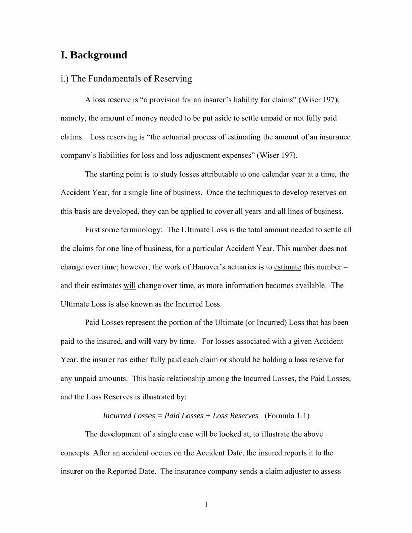
I. Background

i.) The Fundamentals of Reserving

A loss reserve is “a provision for an insurer’s liability for claims” (Wiser 197),

namely, the amount of money needed to be put aside to settle unpaid or not fully paid

claims. Loss reserving is “the actuarial process of estimating the amount of an insurance

company’s liabilities for loss and loss adjustment expenses” (Wiser 197).

The starting point is to study losses attributable to one calendar year at a time, the

Accident Year, for a single line of business. Once the techniques to develop reserves on

this basis are developed, they can be applied to cover all years and all lines of business.

First some terminology: The Ultimate Loss is the total amount needed to settle all

the claims for one line of business, for a particular Accident Year. This number does not

change over time; however, the work of Hanover’s actuaries is to estimate this number –

and their estimates will change over time, as more information becomes available. The

Ultimate Loss is also known as the Incurred Loss.

Paid Losses represent the portion of the Ultimate (or Incurred) Loss that has been

paid to the insured, and will vary by time. For losses associated with a given Accident

Year, the insurer has either fully paid each claim or should be holding a loss reserve for

any unpaid amounts. This basic relationship among the Incurred Losses, the Paid Losses,

and the Loss Reserves is illustrated by:

Incurred Losses = Paid Losses + Loss Reserves (Formula 1.1)

The development of a single case will be looked at, to illustrate the above

concepts. After an accident occurs on the Accident Date, the insured reports it to the

insurer on the Reported Date. The insurance company sends a claim adjuster to assess

1

the loss involved in the case. The claim adjuster’s initial assessment is recorded into the

company’s database on the Recorded Date. The adjuster’s estimate of the loss becomes

the initial Claim Reserve for the case.

There are a number of reasons why Claim Reserves determined in this fashion

may fall short of the total Loss Reserve the insurer should be holding for unpaid losses.

First, it is fairly common for the reported amount of loss on a certain case to change over

time, as it is very hard to make a perfect estimation in a short given period of time. For

this reason, the Hanover actuaries often add a layer of “Supplemental Claim Reserves” to

the Claim Reserves set up by the adjusters. Furthermore, claims associated with a

particular Accident Year are not always known immediately – it can take months or even

years before claims are even reported to the insurer. For these situations, a reserve for

Incurred But Not Reported losses, or IBNR, is calculated and held as an additional

reserve on the insurer’s books. The Incurred Loss can now be presented as:

Incurred Loss = Paid Loss + Claim Reserves + IBNR (Formula 1.2)

To further demonstrate how all the pieces of the Incurred Losses come together,

consider Figure 1.1. This figure shows the Ultimate Loss for claims from an unspecified

line of business for the 2001 Accident Year, broken into sub-components on three

measurement dates. At each measurement date, the Ultimate Loss consists of five pieces:

1. Paid Losses, shown in pink

2. Claim Reserves, shown in tan

3. Supplemental Claim Reserves, shown in yellow.

4. Incurred But Not Reported reserves, shown in green.

5. Error, shown in blue.

2

Notice that as of the initial measurement date, December 31, 2001, a relatively

small portion of the eventual Ultimate Loss has been paid (the pink box). The tan and

yellow boxes are the estimated amounts which will eventually be paid for claims which

have been reported but not yet paid. The green box represents claims which were

incurred during the Accident Year 2001 but have not yet been reported to the insurer.

The blue box represents the total error in the estimates – it is the balancing item to make

sure the pieces sum to the total. The goal of Hanover’s actuaries is to minimize the size

of the blue box.

The second box shows the development of the same Accident Year four years

later, as of December 31, 2005. Paid losses have increased and IBNR has decreased –

and the “error” has decreased, too, since more information is available about the 2001

Accident Year at this point. The magnitude of claim reserves at this point is a function of

how quickly claims are paid once they have been reported.

Eventually, the illustration of Ultimate Loss reaches the stage as shown below as

of December 31, 2036 – at some point, all of the claims are finalized, and the Ultimate

Loss consists only of paid losses.

Paid Losses IBNR Case Reserves Error Supplemental Case Reserves

IBNR IBNR Error Paid Losses

Error

Paid Losses Paid Losses

12/31/2001 12/31/2005 12/31/2036

Figure 1.1

3

Loss Reserving is very important to a property & casualty insurance company.

“Insurance companies must plan for the future (Garrell, Lee 3).” Loss reserving is a vital

part of that process. “The financial condition of an insurance company can not be

adequately assessed without sound loss reserve estimates (Wiser 197).” The concepts

introduced in this section are the basics of the loss reserving process.

4

ii.) Loss Reserve Triangles

The loss reserving triangle is the standard method for maintaining loss data.

While the entries vary for different methods, the use of the triangles is always the same.

12 months 24 months 36 months 48 months 60 months 2001 59,500 70,400 71,700 72,000 71,900 2002 64,200 76,700 77,600 77,700 2003 58,400 72,800 73,900 2004 48,000 58,900 2005 41,300

Table 1.1

Table 1.1 shows the Incurred losses for a certain line of business for Accident

Years 2001 through 2005. As time passes, for a given Accident Year, more claims are

reported or their amounts are adjusted. This accounts for the changes in the Net Incurred

Losses across each row. The columns show the Net Incurred Losses as of a certain stage

in development, in this case every 12 months for each Accident Year. For example, the

value 59,500 is the Net Incurred Loss for Accident Year 2001 after one year of

development while 71,900 is the Net Incurred Loss for the same Accident Year at five

years of development.

Given a loss triangle, one can develop “link ratios”. A link ratio is simply the ratio

of the value for development period Z+1 to development period Z for each Accident

Year. Table 1.2 shows the link ratios for losses in Table 1.1.

12-24 24-36 36-48 48-60 60-Ultimate 2001 1.1832 1.0185 1.0042 0.9986 2002 1.1947 1.0117 1.0013 2003 1.2466 1.0264 2004 1.2271 2005

Table 1.2

5

hese link ratios show the change in losses as they develop. Column “12-24”

displays the ratios of the 24-month developed losses to the 12-month developed losses,

“24-36” for the ratio of the 36-month losses to the 24-month losses, and so on. For

example, during the period between 12 months and 24 months of development for the

2003 accident year, there is an increase in the total incurred cost of losses of 124.66%.

That is, the value of losses incurred during the accident year 2003 after 24 months of

development, 72,800, is 1.2466 times the value after 12 months, 58,400. This table

assumes that growth finished shortly after 60 months, likely by the 72-months

development period. Different lines of business have different development periods – the

example illustrated above has a fairly short “tail”. For lines of business with longer tails,

the link ratio table will extend further to the right, and the values will converge to 1.000

much later.

Given all of the link ratios for the data, there are a number of ways to choose a

link ratio to be used for predicting future loss development. One approach is to take an

average of the calculated link ratios. This could be done as a weighted average of the link

ratios for all years, an average of the most recent 3 years of link ratios, or a weighted

average of the last three years of link ratios. The weighted average takes the sum of the

incurred loss values for next period divided by the sum of the incurred loss values for the

current period. That is, the weighted average over all years for 12-24 months would be:

24 month developed incurred losses 12 month developed incurred losses

212.1000,48400,58200,64500,59900,58700,72700,76700,70

=++++++ or

The following table shows various averages for the data in the example:

6

Age in months: 12-24 24-36 36-48 48-60

all yrs wtd avg 1.212 1.015 1.003 1.000 3 yr avg 1.223 1.015 1.003 1.000

3 yr wtd avg 1.222 1.015 1.003 1.000 select 1.220 1.015 1.003 1.000 1.000

ldf 1.242 1.018 1.003 1.000 1.000 cumulative 80.5% 98.2% 99.7% 100.0% segmented 80.5% 17.7% 1.5% 0.3%

all yrs wtd avg 1.212 1.015 1.003 1.000

Table 1.3

Once the averages have all been calculated, the actuary compares the various link

ratio averages and determines which link ratio to use to estimate development in future

years. The actuary’s choice is known as the “select” link ratio. For the 12-24 month

period, the averages are 1.212, 1.223, and 1.222. The “select” ratio in this example was

1.220. For the 24-36, 36-48, and 48-60, the averages are all the same to three decimal

points, allowing for easy decision making for the select link ratios to be used for future

development. It should be noted that this is not something that usually occurs.

Once the select link ratios are known, they can be used for future loss

development. To do this, the link ratio for the development period is applied to the

incurred loss as of the prior period. The resulting estimates are shown below in Table 1.4:

Development Age (Months) AY 12 24 36 48 60

2001 59,500 70,400 71,700 72,000 71,900 2002 64,200 76,700 77,600 77,700 77,768 2003 58,400 72,000 73,900 74,182 74,199 2004 48,000 58,900 59,077 59,254 59,268 2005 41,300 50,368 51,142 51,295 51,307

Table 1.4

For example, applying the 24-36 month select ratio of 1.015 to the 24-month

losses of 58,900 for the 2004 Accident Year leads to a projected 36-month loss of 59,077.

All of the numbers highlighted in yellow are projected losses.

7

Hanover’s actuaries use a variety of projection methods to project the Ultimate

Loss for a given Accident Year. These methods are discussed in more detail later in this

report. All of the methods use the above link ratio approach in some fashion to develop

their projections of Ultimate Losses.

8

iii.) Basic Projection Methods

Hanover uses six methods to project or predict the Ultimate Losses for a given

Accident Year for each line of business. These methods are:

1. Incurred Method

2. Paid Method

3. Berquist Sherman Paid Method

4. Berquist Sherman Incurred Method

5. Bornhuetter Ferguson Paid Method

6. Bornhuetter Ferguson Incurred Method

These methods are described in more detail below. As noted above, the goal of

each of these methods is to give a projection of the Ultimate Loss for a given Accident

Year. Given this projection, as well as values for Paid Losses and Claim Reserves, it is

possible to develop estimates for the IBNR – a key element for year-end financial

reporting.

a.) Incurred Method

The Incurred Method projects Ultimate Losses based upon losses incurred to date,

assuming that historical incurred loss data will be predictive of future incurred losses.

This method is commonly used due to its ability to use case reserve estimate, which are

developed by the claims adjusters on a case by case basis. However, by using the claims

adjuster’s estimates, it is possible to obtain inaccurate data if the reserve estimates chosen

by the adjusters are not accurate and consistent over time.

9

The accuracy of the incurred method relies on the accuracy of the case reserve

estimates developed by the adjusters, and upon losses occurring in similar patterns for

each Accident Year, over time. If estimates are not reliably determined from year to

year, or if the pattern of loss emergence changes over time, the incurred method will fail

as prior years of incurred data will not accurately predict future years. If the adjusters are

accurate in their reserve estimates, and if loss development is consistent, the incurred

method will develop accurate estimates of ultimate incurred losses.

The Incurred Loss Development Method utilizes the total incurred losses.

Incurred losses, as noted previously, are the total of the paid losses and projected loss

reserves. The loss reserve triangle shown below in Table 1.5 is the start of an example of

the incurred method:

Development Age (Months)

AY 12 24 36 48 60 2001 59,500 70,400 71,700 72,000 71,900 2002 64,200 76,700 77,600 77,700 2003 58,400 72,000 73,900 2004 48,000 58,900 2005 41,300

Assume that no further losses are paid after 60 months

Table 1.5

By analyzing this table, some trends can be seen. Although only 5 years worth of

data is present, it can be seen that since 2002, the amount of incurred losses in the first 12

months of the accident year has been steadily declining. This could be the result of a

decline in the volume of the business. It could also be a result of less conservative loss

reserve estimation in the claims department, with adjusters developing lower reserve

estimates than in the past. Also, both the 24 and 36 month columns (the cumulative

10

incurred losses after 24 months of the accident year and 36 months of the accident year

respectively) show the same trend of a decrease since 2002.

Starting from here, the ultimate losses can be projected by the incurred method

using the link ratio approach in the previous section.

b.) Paid Method

The Paid method also projects ultimate losses from losses paid to date based on

historical development patterns. The actuary uses the record of actual loss payments and

disregards the case reserves. The precision of this reserving technique depends on the

consistency in loss settlement patterns. Change in the rate of inflation, which affect loss

payments, or shifts in can company procedures that influence settlement patterns, can all

cause ambiguity in this reserving method.

c.) Berquist Sherman Methods

The Berquist-Sherman Paid and Incurred methods, sometimes simply called the

Adjusted Paid and Incurred, account for the changes in the way the firm conducts

business from period to period. The methods restate the raw data so that the current

Calendar Year remains unaltered, but previous years are adjusted according to the way

business is conducted. Once restated losses have been attained, the link ratio method as

seen in the regular Paid and Incurred methods is carried out.

In order to find the restated incurred losses, we begin by finding the average loss

amount per claim. To do this, we divide the total of outstanding losses by the number of

outstanding claims. An example of this is shown in Table 1.6.

11

Net Outstanding

Losses

Net Outstanding

Claims

Average Net Outstanding

Losses 1994 50,900 6,700 7,597 1995 48,000 6,940 6,916 1996 53,500 7,160 7,472 1997 59,500 7,140 8,333 1998 52,600 6,850 7,679 1999 44,600 6,540 6,820

Table 1.6

From here, the Average Net Outstanding Claims (ANOC) is adjusted according to

the Selected Trend, a value given by the claims department that is meant to reflect a

line’s inflation. The most recent year’s ANOC is left “as is”, and all prior years are

replaced by this value discounted by the Selected Trend (Table 1.7).

(Trend Factor = 4.0%)

Current ANOC Discount Factor

Discount Factor

Restated Average OS

Claim 1994 6,820 (1.04)^5 1.2167 5605.54 1995 6,820 (1.04)^4 1.1699 5829.76 1996 6,820 (1.04)^3 1.1249 6062.96 1997 6,820 (1.04)^2 1.0816 6305.47 1998 6,820 (1.04)^1 1.0400 6557.69 1999 6,820 (1.04)^0 1.0000 6820.00

Table 1.7

Once the Restated Average Outstanding Claim value is determined, the Restated

Outstanding Losses can be obtained by multiplying the Restated Average by the number

of outstanding claims (Table 1.8).

Restated Average

Outstanding Claim Net Outstanding

Claims Restated

Outstanding Losses 1994 5605.54 6,700 37,557,137 1995 5829.76 6,940 40,458,566 1996 6062.96 7,160 43,410,759 1997 6305.47 7,140 45,021,080 1998 6557.69 6,850 44,920,192 1999 6820 6,540 44,602,800

Table 1.8

12

Finally, to get the Restated Incurred Losses, the Restated Outstanding Losses are

added to the corresponding Paid Losses (Table 1.9).

Paid Losses Restated Outstanding

Losses Restated Incurred

Losses 1994 11000.00 37,557,137 37,568,137 1995 11400.00 40,458,566 40,469,966 1996 11000.00 43,410,759 43,421,759 1997 16900.00 45,021,080 45,037,980 1998 14000.00 44,920,192 44,934,192 1999 10100.00 44,602,800 44,612,900

Table 1.9

Using this procedure across all the data in question produces the Restated

Incurred Loss triangle. As previously noted, the technique for developing a prediction

from a loss triangle using link ratios is known.

For the paid losses, the first step is finding the ratio of the number of Outstanding

Claims to the number of Incurred Claims (Table 1.10).

Number of Outstanding

Claims

Number of Incurred Claims

OS Claims / Incurred Claims

1994 6,700 12,823 0.52 1995 6,940 13,949 0.50 1996 7,160 14,772 0.48 1997 7,140 15,474 0.46 1998 6,850 14,893 0.46 1999 6,540 14,049 0.47

Table 1.10

A new set of ratios is obtained, by dividing the difference for the most current

Accident Year by all of the differences of the years being adjusted, resulting in a set of

Adjustment Ratios (Table 1.11).

13

OS Claims / Incurred

Claims 1 – OS/Inc Claims Adjustment Ratio 1994 0.52 0.48 1.12 1995 0.50 0.50 1.06 1996 0.48 0.52 1.04 1997 0.46 0.54 0.99 1998 0.46 0.54 0.99 1999 0.47 0.53 1.00

Table 1.11

Next, Paid Losses are multiplied by the Adjustment Ratios, leading to the

Restated Paid Losses (Table 1.12). Repeating this process across the entire Paid Losses

triangle gives the Restated Paid Losses triangle, from which link ratios can be developed.

Adjustment

Ratio Raw Paid

Losses Restated Paid

Losses 1994 1.12 11,000 12,313 1995 1.06 11,400 12,126 1996 1.04 11,000 11,410 1997 0.99 16,900 16,772 1998 0.99 14,000 13,856 1999 1.00 10,100 10,100

Table 1.12

The Berquist-Sherman method is useful in situations where there is a discernable

shift in losses as a result of changes in how business is conducted. Trends such as a

slowdown in settlement or payment rate often indicate a line of business as a candidate

for these methods.

d.) Bornheutter Ferguson Method

The Bornheutter-Ferguson Method (BHF) is a method for estimating IBNR

claims and, ultimately, loss reserves based on Estimated Ultimate Losses. It is built off of

an estimation of expected losses, a value derived from the accident year’s earned

14

premium and the line of business’s Estimated Loss Ratio for the year to eliminate the

effect of irregularly large or small claims. As such, the BHF method is put to best use on

lines of business that have a history of being volatile or, in fact, relatively little history at

all. As the goal of the BHF method is to stabilize the data, instead of using incurred or

paid values, which, depending on the line of business, could very likely fluctuate, the

BHF method calculates the Estimated Ultimate Losses as a percentage of the Earned

Annual Premium, which is the total premium the company receives for this particular line

of business.

There are two ways to arrive at results under BHF: the paid and incurred methods.

As the development periods progress, the paid and incurred methods approach the same

value. Because the steps for both methods are the same, only the incurred method will be

shown in example. The paid method can be developed by applying the same steps to the

paid information.

As previously discussed, the BHF method is based upon the line of business’s

Estimated Ultimate Losses. This value is calculated by multiplying the Estimated Loss

Ratio by the respective Annual Earned Premium for the accident year. Both values are

inputs depending on the line of business. An example is shown in Table 1.13.

Estimated Annual Estimated Accident Loss Earned Ultimate

Year Ratio Premium Losses 2001 75.0% 90,900 68,175 2002 80.0% 102,400 81,920 2003 70.0% 107,200 75,040 2004 70.0% 102,800 71,960 2005 60.0% 94,700 56,820

Table 1.13

15

The next step is to determine the IBNR Factors. These values are used to take the

Estimated Ultimate Loss value and determine the Expected IBNR value for each method.

for the incurred method, it is necessary to refer to the Loss Development Factor (LDF)

for the unadjusted incurred method. The LDF is the ratio that transforms the current

incurred value in the loss development triangle to the ultimate value. The IBNR Factor is

determined by Formula 1.3 and an example is given in Table 1.14.

LDFFactorIBNR 11_ −= (Formula 1.3)

Estimated Annual Estimated Incurred Accident Loss Earned Ultimate IBNR

Year Ratio Premium Losses Factor 2001 75.0% 90,900 68,175 0.000 2002 80.0% 102,400 81,920 0.000 2003 70.0% 107,200 75,040 0.003 2004 70.0% 102,800 71,960 0.018 2005 60.0% 94,700 56,820 0.195

Table 1.14

The same steps are undertaken to develop the IBNR Factor for the paid method

with the LDF from the unadjusted paid loss development triangle. In order to determine

the Estimated IBNR for the incurred method, the IBNR Factor (Incurred) is multiplied by

the Estimate Ultimate Loss value, as shown in Table 1.15. Similarly, for the Estimated

IBNR for the paid method, the IBNR Factor (Paid) is used.

Estimated Annual Estimated Incurred Expected Accident Loss ratio Earned Ultimate IBNR Incurred

Year Ratio Premium Losses Factor IBNR 2001 75.0% 90,900 68,175 0.000 0 2002 80.0% 102,400 81,920 0.000 19 2003 70.0% 107,200 75,040 0.003 242 2004 70.0% 102,800 71,960 0.018 1,292 2005 60.0% 94,700 56,820 0.195 11,083

Table 1.15

16

iv.) The Four Lines of Business

Hanover Insurance is primarily a property and casualty insurer, meaning that most

of their business is in automobile and property insurance, both for individuals and for

businesses. The four lines of business included in this report are: Business Owners

Policy Liability, Commercial Auto Liability, Personal Auto Bodily Injury, and Personal

Auto Property Damage Liability. These are discussed briefly below.

a.) Business Owners Policy Liability

This kind of insurance contract is offered to small or medium-sized businesses to

protect their buildings and personal property. The policies may also include business

income, extra expense coverage, and other common coverages, such as employee

dishonesty, money and securities, and equipment.

b.) Commercial Auto Liability

This kind of insurance is offered to small or large businesses providing protection

for losses resulting from operating an auto. The insurance covers bodily injury and

property damage for which the insured is liable as a result of operating vehicles.

c.) Personal Auto Bodily Injury

This kind of insurance covers bodily injuries or death for which the insured is

responsible. It pays for medical bills, loss of income or pain and suffering of another

party, and legal defense for the insured if necessary.

d.) Personal Auto Property Damage Liability

This kind of insurance covers the property damages the insured caused to another

party in a car accident, and it also includes legal defense.

17

v.) Paid Losses Development Analysis

Hanover provided data for the four line of business mentioned previously for

year-end loss reserve analysis for calendar years 1996 through 2001. In total, there are

twenty-four Excel files, one for each of six calendar years for each of the four lines of

business. The data in these files range from Accident Year 1981 through 2001. After

review of the data, the Accident Years 1981 to 1988 were considered fully developed by

the end of 2001, and the following discussion focuses on these Accident Years.

a.) Basic Analysis

First some basic properties of the four lines of businesses were studied. Table

1.16 and Figure 1.2 show the Ultimate Losses for these years, for each of the four lines of

business. It is clear that PABI > CAL > PAPD > BOP for the Ultimate Losses across

almost all these accident years. This shows the magnitude of the various lines in terms of

incurred losses. Further, BOP > CAL > PABI > PAPD in terms of percentage growth

over 1981-88, with a minimum of 83% increase for PAPD, and up to 1660% increase for

BOP. This indicates the lines of business are growing most rapidly over the study period.

Accident Year BOP CAL PABI PAPD 1981 750 11,600 23,500 12,600 1982 1,500 16,500 30,600 13,600 1983 1,800 16,100 35,400 14,600 1984 3,200 27,500 42,100 17,000 1985 7,200 31,100 45,000 20,000 1986 4,800 32,700 47,800 21,300 1987 7,800 38,800 49,400 22,500 1988 13,300 37,100 58,100 23,100

Table 1.16

18

Ultimate Loss Amounts 1981 - 1988

010,00020,00030,000

40,00050,00060,00070,000

1981 1982 1983 1984 1985 1986 1987 1988

Accident Year

Ultim

ate

Loss

es BOPCALPABIPAPD

Figure 1.2

Average AY 1981 - 1988

0%

20%

40%

60%

80%

100%

120%

1 2 3 4 5 6 7 8 9 10 11 12 13 14 15 16

Development Age

Per

cent

age BOP

CALPABIPAPD

Figure 1.3

Annual Increment on the Average 1981 - 1988

-10%0%

10%20%30%40%50%60%70%80%

1 2 3 4 5 6 7 8 9 10 11 12 13 14 15 16

Development Age

Perc

enta

ge C

hang

e

BOPCALPABIPAPD

Figure 1.4

19

Figure 1.3 and Figure 1.4 show a comparison of the average amount of these eight

accident years, indicated by “development age”. From the annual increment chart it can

be seen that PAPD had a large first year paid loss amount, an increment of about one-

third of that in the second year, and finished off soon after that. Both PABI and BOP had

peak(s) of increments. PABI had a single-mode graph, of which the peak resides around 2

years after the accident year, where BOP was of multi-mode, year 2, 4, 6 of the

development are all little peaks. The increasing rate of the CAL line slowed down over

time as PAPD, but with a much flatter slope.

Standard Deviations by Development Ages

0%

2%

4%

6%

8%

10%

1 2 3 4 5 6 7 8 9 10 11 12 13 14 15 16

Development Age

Stan

dard

Dev

iatio

n

BOPCALPABIPAPD

Figure 1.5

Standard deviations were calculated for each development age of these accident

years (Figure 1.5). As a percentage of development, the standard deviations follow the

pattern BOP > CAL > PABI > PAPD, especially for the first 7 years of development.

BOP was the most unstable (highest standard deviation), and PAPD was the most stable.

Another important item to look at is the correlation between different lines of

business. Figure 1.6 shows the correlation of different lines of business in different

20

accident years. CAL and PABI are the most related. The lines BPL, CAL, and PABI are

fairly closely related. Correlations with PAPD are not as strong as with the other lines.

Correlation by Accident Year

60%65%70%75%80%85%90%95%

100%

1981 1982 1983 1984 1985 1986 1987 1988

Accident Year

Corr

elat

ion

BOP vs CALBOP vs PABIBOP vs PAPDCAL vs PABICAL vs PAPDPABI vs PAPD

Figure 1.6

Table 1.17 summarizes what was stated above, giving a rank of 1 to the strongest

condition and 4 to the weakest.

BOP CAL PABI PAPD Ultimate Loss 4 2 1 3

Increment of Ultimate Loss 1 2 3 4 Variance 1 2 3 4

Years to Ultimate 13 - 14 14 - 15 11 – 12 5 - 6

Table 1.17

b.) Analysis by Lines of Business

Another way to look at the data is by line of business. The data provides the

development through a number of years. The Ultimate Loss is taken as Hanover’s

recorded or projected Ultimate Loss as of the end of the 2001 accident year. From this, a

percentage is calculated by dividing the known losses (paid losses plus claim reserves) as

of a certain development period by the Ultimate Loss. Percentages are used instead of

21

dollar amounts since each line of business experiences different magnitudes of claims,

and over the years the magnitude of claims for a certain line of business can vary. This

approach results in a data set that gives the cumulative “percentage of ultimate” for each

line of business by development age.

As can be seen in Figure 1.7 and Table 1.18, paid losses for BOP did not develop

a consistent pattern over time. The graphs for different accident years stay at a distance

from each other, and the standard deviations in the table are large. The paid losses start

from a low point (around 10% or 12%), and develop very slowly for 13 to 14 years

before reaching ultimate.

Business Owners Policy Liability 1981 - 1988

0%

20%

40%

60%

80%

100%

120%

1 2 3 4 5 6 7 8 9 10 11 12 13 14 15 16

Development Age

Per

cent

age

of U

ltim

ate

Loss 1981

1982198319841985198619871988

Figure 1.7

BOP 1 2 3 4 5 6 7 8 9 10 11 12 13 14

Mean 10% 31% 48% 67% 79% 91% 94% 97% 98% 99% 99% 100% 100% 100%

SD 4% 7% 9% 9% 8% 4% 4% 3% 2% 2% 1% 1% 0% 0%

Table 1.18

22

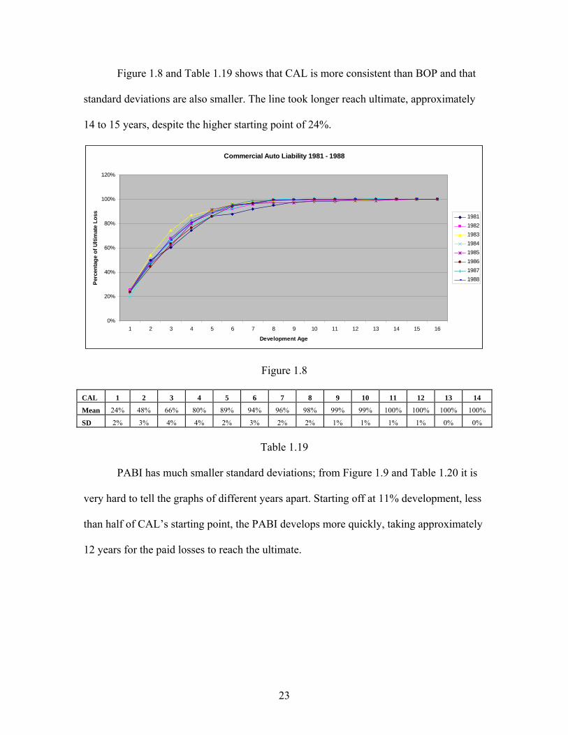
Figure 1.8 and Table 1.19 shows that CAL is more consistent than BOP and that

standard deviations are also smaller. The line took longer reach ultimate, approximately

14 to 15 years, despite the higher starting point of 24%.

Commercial Auto Liability 1981 - 1988

0%

20%

40%

60%

80%

100%

120%

1 2 3 4 5 6 7 8 9 10 11 12 13 14 15 16

Development Age

Perc

enta

ge o

f Ulti

mat

e Lo

ss 19811982198319841985198619871988

Figure 1.8

CAL 1 2 3 4 5 6 7 8 9 10 11 12 13 14

Mean 24% 48% 66% 80% 89% 94% 96% 98% 99% 99% 100% 100% 100% 100%

SD 2% 3% 4% 4% 2% 3% 2% 2% 1% 1% 1% 1% 0% 0%

Table 1.19

PABI has much smaller standard deviations; from Figure 1.9 and Table 1.20 it is

very hard to tell the graphs of different years apart. Starting off at 11% development, less

than half of CAL’s starting point, the PABI develops more quickly, taking approximately

12 years for the paid losses to reach the ultimate.

23

Personal Auto Bodily Injury 1981 - 1988

0%

20%

40%

60%

80%

100%

120%

1 2 3 4 5 6 7 8 9 10 11 12 13 14 15 16

Development Age

Perc

enta

ge o

f Ulti

mat

e Lo

ss 19811982198319841985198619871988

Figure 1.9

PABI 1 2 3 4 5 6 7 8 9 10 11 12 13 14

Mean 11% 41% 65% 81% 91% 96% 98% 99% 100% 100% 100% 100% 100% 100%

SD 1% 2% 2% 2% 1% 1% 1% 1% 1% 0% 0% 0% 0% 0%

Table 1.20

PAPD clearly stands out among the four lines of business. With very small

standard deviations, the differences between graphs are almost invisible. This line fully

develops within about six years, much more quickly than any of the other lines.

24

Personal Auto Property Damage Liability 1981 - 1988

0%

20%

40%

60%

80%

100%

120%

1 2 3 4 5 6 7 8 9 10 11 12 13 14 15 16

Development Age

Perc

enta

ge o

f Ulti

mat

e Lo

ss 19811982198319841985198619871988

Figure 1.10

PAPD 1 2 3 4 5 6 7 8 9 10 11 12 13 14

Mean 71% 96% 99% 100% 100% 100% 100% 100% 100% 100% 100% 100% 100% 100%

SD 1% 0% 0% 0% 0% 0% 0% 0% 0% 0% 0% 0% 0% 0%

Table 1.21

25

II. Analysis of Estimated Ultimate Losses

i.) Analysis of Ultimate Losses

The estimated Ultimate Losses from each of the six methods are recalculated

annually as new data comes in. Because this new data is closer to the true Ultimate Loss

over time, it would seem that recalculating estimated values based on this new data

would result in more accurate estimates. This, however, is not always the case. Trends

appearing in the data suggest there are outside factors influencing the changes as well.

Following is a comparative analysis for the four lines of business for the accident

years of 1996 and 1997. A percentage error of the estimated ultimate losses against the

actual ultimate loss value as of 2006 is calculated.

CAL 1996 Ultimate Predictions: % Error from Actual (2006)

-10

-5

0

5

10

15

20

25

1996 1997 1998 1999 2000 2001

Calendar Year

% E

rror

from

Act

ual Incurred

PaidBS IncurredBS PaidBHF IncurredBHF PaidHanover's

Figure 2.1

26

CAL 1997 Ultimate Predictions: % Error from Actual (2006)

-10

-5

0

5

10

15

20

25

1997 1998 1999 2000 2001

Calendar Year

% E

rror

from

Act

ual Incurred

PaidBS IncurredBS PaidBHF IncurredBHF PaidHanover's

Figure 2.2

In Figure 2.1 and Figure 2.2, it can be seen that for CAL the paid methods (Paid,

BS Paid, and BHF Paid) consistently predict ultimate values larger than the actual and,

quite frequently, larger than the incurred methods. Calendar years 1997 and 1998 are

stand-out years for this trend. Hanover’s estimate very closely matches the Incurred

method in 1997, implying that Hanover may have been aware of the Paid methods’

current inaccuracy and thus put more weights on other methods.

BOP 1996 Ultimate Predictions: % Error from Actual (2006)

-30

-20

-10

0

10

20

30

40

50

60

70

1996 1997 1998 1999 2000 2001

Calendar Year

% E

rror

from

Act

ual (

2006

)

IncurredPaidBS IncurredBS PaidBHF IncurredBHF PaidHanover's

Figure 2.3

27

BOP 1997 Ultimate Predictions: % Error from Actual (2006)

-30

-20

-10

0

10

20

30

40

50

60

70

1997 1998 1999 2000 2001

Calendar Year

% E

rror

from

Act

ual (

2006

)

IncurredPaidBS IncurredBS PaidBHF IncurredBHF PaidHanover's

Figure 2.4

In Figure 2.3 and Figure 2.4, the severe overestimation made by the Paid methods

that was seen in the CAL graphs continues to be apparent for BOP. The incurred methods

also show a significant amount of error, particularly the Berquist-Sherman Incurred

method. Hanover’s “select” predictions do not seem to follow any particular method, but

rather are among the various different methods, indicating that there might not be any

historical trends for the accuracy of any of the methods for the BOP line.

PAPD 1996 Ultimate Predictions: % Variance of Actual (2006)

-5

-4

-3

-2

-1

0

1

2

1996 1997 1998 1999 2000 2001

Calendar Year

% V

arianc

e of

Act

ual (20

06)

IncurredPaidBSIncurredBSPaidBHFIncurredBHFPaidHanover's

Figure 2.5

28

PAPD 1997 Ultimate Predictions: % Variance of Actual (2006)

-5

-4

-3

-2

-1

0

1

2

1997 1998 1999 2000 2001

Calendar Year

% V

arianc

e of

Act

ual (20

06)

IncurredPaidBSIncurredBSPaidBHFIncurredBHFPaidHanover's

Figure 2.6

Compared with the other three lines of business, PAPD has a relatively short tail

that approaches full development very quickly – reasonable, since the nature of this line

of business is non-bodily injury with minimal litigation. Within 3-5 years of development

age, all the methods and Hanover’s choice approach 0% error. The Paid method

continues its trend of over-estimating the ultimate, and Hanover chose estimates more in

line with the Incurred methods. However, the short-tail of the line reduces the effect of

any poor estimates as can be seen in Figure 2.5 and Figure 2.6.

PABI 1996 Ultimate Predictions: % Variance of Actual (2006)

-15

-5

5

15

25

35

45

1996 1997 1998 1999 2000 2001

Calendar Year

% V

arianc

e of

Act

ual (20

06)

IncurredPaidBSIncurredBSPaidBHFIncurredBHFPaidHanover's

Figure 2.7

29

PABI 1997 Ultimate Predicitons: % Variance of Actual (2006)

-15

-5

5

15

25

35

45

1997 1998 1999 2000 2001

Calendar Year

% V

aria

nce

of A

ctua

l (20

06)

IncurredPaidBSIncurredBSPaidBHFIncurredBHFPaidHanover's

Figure 2.8

The PABI graphs, Figures 2.7 and 2.8, show the same overarching trends that can

be seen in the other three lines. For one, the Paid methods tend to consistently

overestimate the ultimate losses. Hanover appeared to be aware of this as they chose their

estimates to be closer to the Incurred methods. At 5-6 years of development, all the

methods are approaching 0% error, indicating that near this age, the losses approach full

development.

30

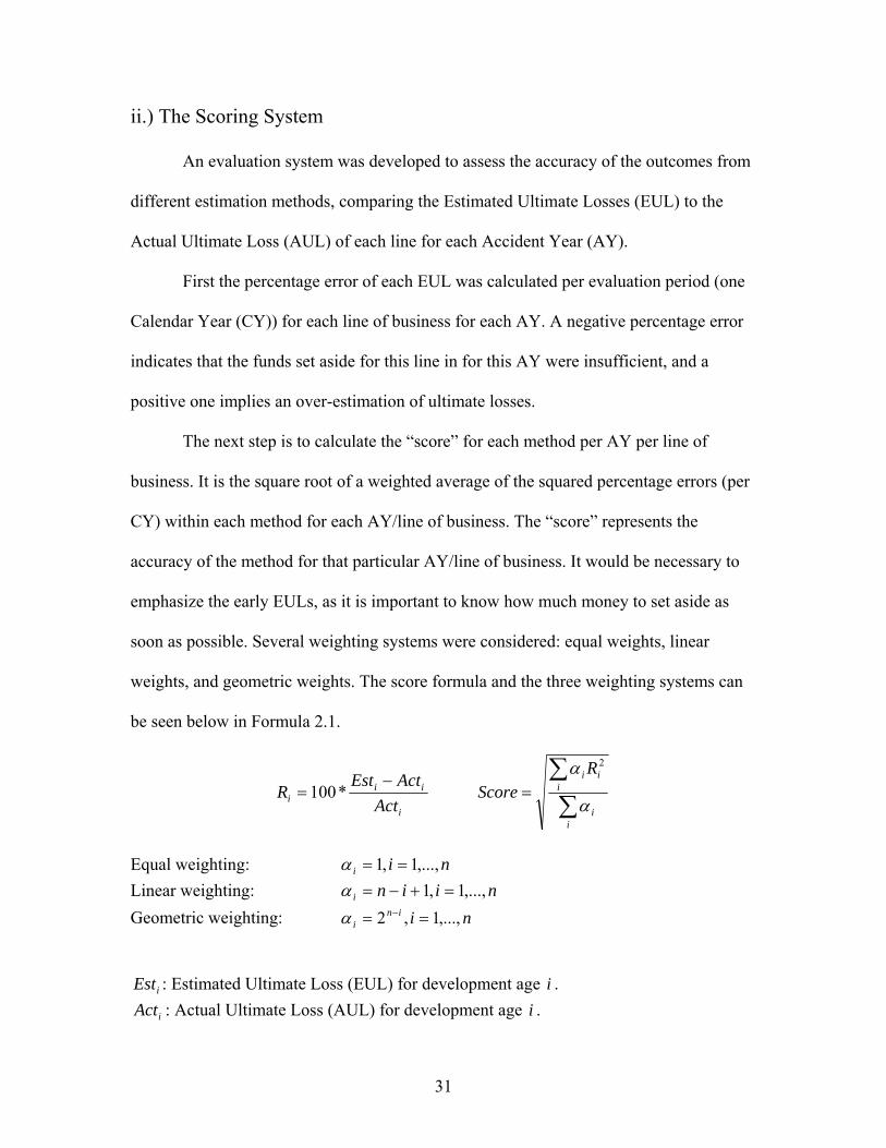
ii.) The Scoring System

An evaluation system was developed to assess the accuracy of the outcomes from

different estimation methods, comparing the Estimated Ultimate Losses (EUL) to the

Actual Ultimate Loss (AUL) of each line for each Accident Year (AY).

First the percentage error of each EUL was calculated per evaluation period (one

Calendar Year (CY)) for each line of business for each AY. A negative percentage error

indicates that the funds set aside for this line in for this AY were insufficient, and a

positive one implies an over-estimation of ultimate losses.

The next step is to calculate the “score” for each method per AY per line of

business. It is the square root of a weighted average of the squared percentage errors (per

CY) within each method for each AY/line of business. The “score” represents the

accuracy of the method for that particular AY/line of business. It would be necessary to

emphasize the early EULs, as it is important to know how much money to set aside as

soon as possible. Several weighting systems were considered: equal weights, linear

weights, and geometric weights. The score formula and the three weighting systems can

be seen below in Formula 2.1.

i

iii Act

ActEstR

−= *100

∑∑

=

ii

iii R

Scoreα

α 2

Equal weighting: nii ,...,1,1 ==α Linear weighting: niini ,...,1,1 =+−=α Geometric weighting: niin

i ,...,1,2 == −α

iEst : Estimated Ultimate Loss (EUL) for development age . i

iAct : Actual Ultimate Loss (AUL) for development age i .

31

iR : Percentage Error for the EUL of development age i .

iα : Weighting for the percentage error of development age i in the final score.

Formula 2.1

The effects of different weighting systems were experimented with the data for

the 1996 AY. The graphs of the results under equal, linear, and geometric weightings are

in Figures 2.9, 2.10, and 2.11 respectively.

IncurredPaid

BSIncurred BS Paid

BHFIncurred BHF Paid

Hanover's

PAPD

CAL

PABI

BOP0.00

5.00

10.00

15.00

20.00

25.00

30.00

35.00

Scores

Methods

Lines of Business

Scores for Different Methods for AY 1996 with Equal Weights

PAPDCALPABIBOP

Figure 2.9

Incurred Paid BSIncurred BS Paid

BHFIncurred BHF Paid

Hanover's

PAPD

CAL

PABI

BOP0.00

5.00

10.00

15.00

20.00

25.00

30.00

35.00

Scores

Methods

Lines of Business

Scores for Different Methods for AY 1996 with Linear Weights

PAPDCALPABIBOP

Figure 2.10

32

IncurredPaid

BSIncurred BS Paid

BHFIncurred BHF Paid

Hanover's

PAPD

CAL

PABI

BOP

0.00

5.00

10.00

15.00

20.00

25.00

30.00

35.00

Scores

Methods

Lines of Business

Scores for Different Methods for AY 1996 with Geometric Weights

Figure 2.11

The geometric weighting system was considered to be most suitable here. It puts

twice as much emphasis on the N-th evaluation period as on the N+1-st. Thus it results in

low scores for estimations that were accurate in early years and high scores for

estimations that were inaccurate in early years. For example, in the figures above, for the

PAPD line, which is very consistent in its growth patterns, the change in score from equal

weighting to linear to geometric is very little. Alternatively, for the BOP line, which has a

larger fluctuation range, the scores tend to grow from equal to linear to geometric

weighting. Table 2.1 below shows the scores for AY 1996, and Table 2.2 shows those for

the PABI line.

AY 1996 CAL BOP PAPD PABI Incurred 7.12 24.11 2.48 7.24 Paid 10.48 32.55 0.86 17.70 BS Incurred 5.98 17.19 2.96 13.66 BS Paid 7.25 20.95 1.70 8.56 BHF Incurred 5.68 15.30 2.56 8.73 BHF Paid 4.92 19.09 1.37 14.17 Hanover's 1.68 17.17 1.37 6.53

Table 2.1

33

PABI 1996 1997 1998 1999 2000 2001 Incurred 7.24 8.08 2.05 9.26 4.88 9.37 Paid 17.70 31.60 16.80 6.98 5.24 4.55 BS Incurred 13.66 6.15 5.72 6.29 2.98 7.62 BS Paid 8.56 12.44 6.35 12.40 3.93 7.78 BHF Incurred 8.73 4.94 2.90 5.24 3.99 7.70 BHF Paid 14.17 5.66 7.09 1.61 2.38 4.21 Hanover's 6.53 7.00 5.71 1.61 0.80 5.95

Table 2.2

From Table 2.1 it is possible to tell that for AY 1996, the Hanover made the best

prediction for the CAL and PABI lines, but the information in Table 2.2 is less clear.

Thus the “rankings” were introduced as a more direct way to evaluate the methods. The

scores for the seven methods per accident year per line of business were extracted and

sorted from low to high, assigning each method a rank from 1 to 7. A “1” corresponds to

the lowest score, indicating the best method for a certain year and line. An example is

shown in Table 2.3 below, rankings for AY 1996 for all four lines.

AY 96 CAL BOP PAPD PABI Score Ranking Score Ranking Score Ranking Score Ranking

Incurred 7.12 5 24.11 6 2.48 5 7.24 2 Paid 10.48 7 32.55 7 0.86 1 17.70 7 BS Incurred 5.98 4 17.19 3 2.96 7 13.66 5 BS Paid 7.25 6 20.95 5 1.70 4 8.56 3 BHF Incurred 5.68 3 15.30 1 2.56 6 8.73 4 BHF Paid 4.92 2 19.09 4 1.37 2 14.17 6 Hanover's 1.68 1 17.17 2 1.37 3 6.53 1

Table 2.3

It is still not clear from these individual rankings if there is a method that works

constantly better for a certain line of business. In Table 2.4 below are the sums of the

rankings across the six accident years for each method, and just to further illustrate, in

Table 2.5 these combined rankings were sorted again. It can be seen that the Hanover

made the best prediction 2 out of 4 lines of business, with BHF Paid standing out in the

34

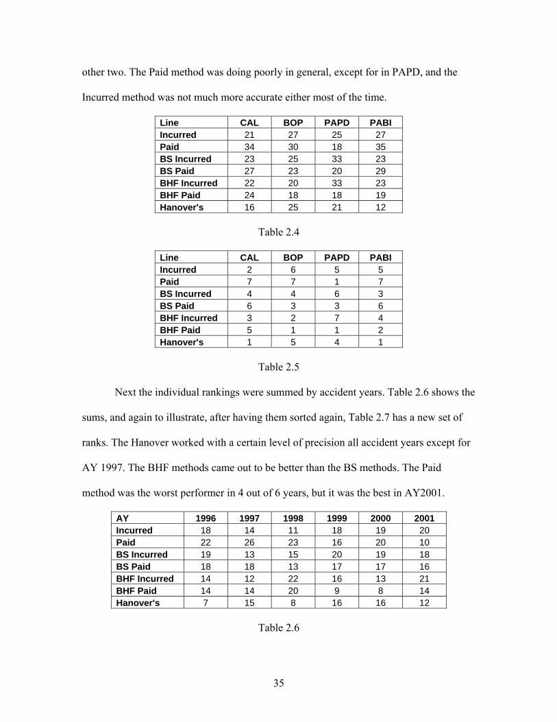
other two. The Paid method was doing poorly in general, except for in PAPD, and the

Incurred method was not much more accurate either most of the time.

Line CAL BOP PAPD PABI Incurred 21 27 25 27 Paid 34 30 18 35 BS Incurred 23 25 33 23 BS Paid 27 23 20 29 BHF Incurred 22 20 33 23 BHF Paid 24 18 18 19 Hanover's 16 25 21 12

Table 2.4

Line CAL BOP PAPD PABI Incurred 2 6 5 5 Paid 7 7 1 7 BS Incurred 4 4 6 3 BS Paid 6 3 3 6 BHF Incurred 3 2 7 4 BHF Paid 5 1 1 2 Hanover's 1 5 4 1

Table 2.5

Next the individual rankings were summed by accident years. Table 2.6 shows the

sums, and again to illustrate, after having them sorted again, Table 2.7 has a new set of

ranks. The Hanover worked with a certain level of precision all accident years except for

AY 1997. The BHF methods came out to be better than the BS methods. The Paid

method was the worst performer in 4 out of 6 years, but it was the best in AY2001.

AY 1996 1997 1998 1999 2000 2001 Incurred 18 14 11 18 19 20 Paid 22 26 23 16 20 10 BS Incurred 19 13 15 20 19 18 BS Paid 18 18 13 17 17 16 BHF Incurred 14 12 22 16 13 21 BHF Paid 14 14 20 9 8 14 Hanover's 7 15 8 16 16 12

Table 2.6

35

AY 1996 1997 1998 1999 2000 2001 Incurred 4 4 2 6 6 6 Paid 7 7 7 4 7 1 BS Incurred 6 2 4 7 5 5 BS Paid 5 6 3 5 4 4 BHF Incurred 2 1 6 2 2 7 BHF Paid 3 3 5 1 1 3 Hanover's 1 5 1 3 3 2

Table 2.7

To have a general idea of which method performed best across the six accident

years and four lines of business, the individual rankings were summed to have a total

ranking for each method, as is shown below in Table 2.8. The Hanover gave the best

results overall and the Paid method the poorest. The BHF methods ranked the 2nd and the

3rd, and the Incurred method outperformed the BS Incurred, which was not readily

apparent in previous tables.

Incurred Paid BS

IncurredBS

Paid BHF

IncurredBHF Paid Hanover's

Total 100 117 104 99 98 79 74 Rank 5 7 6 4 3 2 1

Table 2.8

36

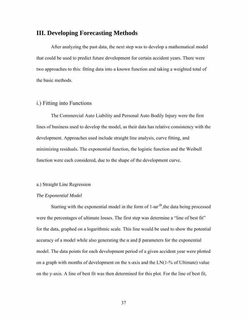
III. Developing Forecasting Methods

After analyzing the past data, the next step was to develop a mathematical model

that could be used to predict future development for certain accident years. There were

two approaches to this: fitting data into a known function and taking a weighted total of

the basic methods.

i.) Fitting into Functions

The Commercial Auto Liability and Personal Auto Bodily Injury were the first

lines of business used to develop the model, as their data has relative consistency with the

development. Approaches used include straight line analysis, curve fitting, and

minimizing residuals. The exponential function, the logistic function and the Weibull

function were each considered, due to the shape of the development curve.

a.) Straight Line Regression

The Exponential Model

Starting with the exponential model in the form of 1-αe-βt,the data being processed

were the percentages of ultimate losses. The first step was determine a “line of best fit”

for the data, graphed on a logarithmic scale. This line would be used to show the potential

accuracy of a model while also generating the α and β parameters for the exponential

model. The data points for each development period of a given accident year were plotted

on a graph with months of development on the x-axis and the LN(1-% of Ultimate) value

on the y-axis. A line of best fit was then determined for this plot. For the line of best fit,

37

y=mx+b, the parameters m and b were determined. To transform back to the exponential

model, α = eb, and β = -m.

Given α and β, the exponential model is dependent solely upon time. As an

example, the 1989 accident year for Commercial Auto Liability paid data had a line of

best fit of y=-0.5177x - 0.0691, resulting in f(t)=1-1.0715e-0.5177t. The following table

shows actual percentage development side by side with the projected development.

Months CAL Ultimate AY1989 % Model % 12 9,582 40,200 23.8% 36.3% 24 19,203 40,200 47.8% 62.0% 36 29,298 40,200 72.9% 77.4% 48 34,830 40,200 86.6% 86.5% 60 37,200 40,200 92.5% 92.0% 72 38,277 40,200 95.2% 95.2% 84 39,325 40,200 97.8% 97.1% 96 39,675 40,200 98.7% 98.3% 108 39,981 40,200 99.5% 99.0% 120 40,046 40,200 99.6% 99.4% 132 40,079 40,200 99.7% 99.6% 144 40,079 40,200 99.7% 99.8% 156 40,080 40,200 99.7% 99.9%

Table 3.1

Commercial Auto Liability

-7

-6

-5

-4

-3

-2

-1

01 2 3 4 5 6 7 8 9 10 11 12 13

Months of Development

LN(1

-% o

f Ulti

mat

e) AY1989

Linear(AY1989)

Figure 3.1

38

In Figure 3.1, the data from the column AY1989 % of Ultimate is shown with the

purple stars. The line of best fit is then fit based on this data. Once the Model %’s of

Ultimate are known, a graph can be produced to show the actual % of ultimate for the

accident year as well as the model’s projection. Figure 3.2 below displays AY 1989 CAL

paid development. Actual data is shown by a dark red dot and the model is shown with a

purple line.

Commercial Auto Liability

0.0%

20.0%

40.0%

60.0%

80.0%

100.0%

120.0%

12 24 36 48 60 72 84 96 108 120 132 144 156

Months of Development

% o

f Ulti

mat

e AY1989

expmodel

Figure 3.2

There appears to be a very good fit to the data, suggesting that a mathematical

approach to loss reserve estimation may be possible. The model projects that the 12

month development is approximately 36% of the eventual ultimate, which is a very good

fit to the actual numbers. However, the majority of the years are not this consistent.

Shown below in Figure 3.3 is the exponential model for the accident year 1991 paid data

for Commercial Auto Liability. The model predicts that the 12 month development will

be approximately 13% of the ultimate. However, the actual development shows that the

39

12 month development is approximately 27% of the ultimate. This poor result eliminates

the model’s usefulness.

Commercial Auto Liability

0.0%

20.0%

40.0%

60.0%

80.0%

100.0%

120.0%

12 24 36 48 60 72 84 96 108 120 132 144 156

Months of Development

% o

f Ulti

mat

e expmodel

AY1991

Figure 3.3

If the above model were to be used, we would actually over project our ultimate

losses by nearly 200%. This inconsistency in the model’s forecasting ability exists across

all lines of business.

An additional question that arises with the development of the models is that

when applied to 13 different accident years, it results 13 different α value parameters and

13 different β value parameters. The problem then becomes one of deciding which α and

β values to use to generate a consistent model for the future.

The Logistic Model

The next model was the logistic model, 1( )1 ktf t

eβ −=+

.

40

LN((1/% of Ultimate)-1) was plotted against months of development. The line of

best fit was determined as y = mx+b. To convert from the linear model back to the

logistic model, β = eb, and k = -m.

For example, the 1989 accident year for Commercial Auto Liability paid data had

a line of best fit of y=-0.5767x-0.0165, leading to tetf 5767.0167.11

1)( −+= . The

following table shows actual percentage development side by side with the projected

development.

Months CAL Ultimate AY1989 % Model % 12 9,582 40,200 23.8% 36.3% 24 19,203 40,200 47.8% 62.0% 36 29,298 40,200 72.9% 77.4% 48 34,830 40,200 86.6% 86.5% 60 37,200 40,200 92.5% 92.0% 72 38,277 40,200 95.2% 95.2% 84 39,325 40,200 97.8% 97.1% 96 39,675 40,200 98.7% 98.3% 108 39,981 40,200 99.5% 99.0% 120 40,046 40,200 99.6% 99.4% 132 40,079 40,200 99.7% 99.6% 144 40,079 40,200 99.7% 99.8% 156 40,080 40,200 99.7% 99.9%

Table 3.2

Commercial Auto Liability

-8

-7

-6

-5

-4

-3

-2

-1

0

1

2

1 2 3 4 5 6 7 8 9 10 11 12 13

Months of Development

LN(1

/ % o

f Ulti

mat

e-1)

AY1989

Linear(AY1989)

Figure 3.4

41

In Figure 3.4, the data from the column AY1989 % of Ultimate is shown with the

purple stars. The line of best fit is then fit based on this data. In Figure 3.5 below, the %

of ultimate for actual data is shown by a dark red dot and the model is shown with a

purple line.

Commercial Auto Liability

0.0%

20.0%

40.0%

60.0%

80.0%

100.0%

120.0%

12 24 36 48 60 72 84 96 108 120 132 144 156

Months of Development

% o

f Ulti

mat

e

AY1989

logisticmodel

Figure 3.5

This model predicts that the development at 12 months is approximately 36% of

the ultimate. The actual data shows it is approximately 23% of the ultimate. However, the

majority of the years in the paid loss data could be more consistent. Shown below in

Figure 3.6 is the logistic model for the accident year 1992 paid data for Commercial Auto

Liability. The model predicts that the 12 month development will be approximately 25%

of the ultimate. However, the actual development shows that the 12 month development

is approximately 25.4% of the ultimate. Since the goal is to accurately project the

ultimate after 12 months of development, this is not a good or useable model.

42

Commercial Auto Liability

0.0%

20.0%

40.0%

60.0%

80.0%

100.0%

120.0%

12 24 36 48 60 72 84 96 108 120 132 144 156

Months of Development

% o

f Ulti

mat

e

logisticmodel

AY1992

Figure 3.6

b.) Curve Fitting

Another approach was to build a model by looking for a function whose graph

was closest to the actual data from the past, and testing it with years that were not fully

developed. The formulas of the 3 basic functions, Exponential, Logistic, and Weibull are

as follows,

--- Exponential bteatf −⋅−= 1)(

bmt

etf −

−+

=1

1)( --- Logistic

--- Weibull rtbetf ⋅−−=1)(

where the t is the development age of the business for a particular Accident Year.

First, the percentages of the paid losses to the ultimate losses the first 12 months

and 24 months for CAL were used to calculate a set of values for the two parameters for

43

each function, and then the formulas were used to extrapolate the percentages for later

development ages.

CAL 1 2 A b m 1/b b r 1981 25% 50% 1.1045 0.3933 2.0112 1.0620 0.2939 1.2254 1982 25% 48% 1.0619 0.3529 2.0991 0.9810 0.2928 1.1409 1983 25% 54% 1.2242 0.4890 1.8742 1.2613 0.2867 1.4360 1984 19% 48% 1.2407 0.4301 2.0751 1.3309 0.2144 1.5878 1985 25% 47% 1.0694 0.3489 2.1299 0.9933 0.2818 1.1623 1986 23% 45% 1.0586 0.3238 2.2238 0.9680 0.2669 1.1463 1987 23% 47% 1.1180 0.3760 2.0995 1.0866 0.2645 1.2760 1988 24% 49% 1.1399 0.4027 2.0335 1.1262 0.2718 1.3114

Table 3.3

Comparison of Averages of Functions CAL

0%

20%

40%

60%

80%

100%

120%

1 3 5 7 9 11 13 15

Development age

Perc

enta

ge o

f Ult

Loss

es

ActualLogisticExponentialWeibull

Figure 3.7

The above chart, Figure 3.7 is the average for each development age over eight

accident years. From the graph it is clear that the Weibull function fits almost perfectly

with the data. Therefore Weibull was selected as a model for CAL.

It was obvious that a new set of parameters was needed for each subsequent year.

Further, because paid losses numbers are expressed in real dollars, not in percentages as

when they were plotted, a “standard” percentage number of the paid loss to the ultimate

44

loss for the first 12 months is needed to generate forecasts. Looking at the first 12

months data for each year 1981 to 1988, the numbers had a mean 24% with a standard

deviation of 2%. Thus 24% was selected as the “standard” first year percentage. The

second year percentage number could be obtained once the paid loss for the first 24

months in real dollars was available, %241$2$2 ⋅=

yearyearpercyear . From here and the

percentage numbers for all the development ages of this accident year could be

developed, including the paid losses developing to ultimate, with

rb,

%%24

1$$ yearTyearyearT ⋅= . Examples for certain Accident Years are shown in Figure

3.8 below.

Actual vs Weibull 1989, 1992, 1996 CAL

05000

1000015000200002500030000350004000045000

1 3 5 7 9 11 13 15

Development Age

Paid

Los

ses

1989 Actual1992 Actual1996 Actual1989 Weibull1992 Weibull1996 Weibull

Figure 3.8

The same strategy is used for PABI as with CAL. The parameters were

developed, then the averages were extrapolated and compared. However, no one of the

three functions worked well for PABI. After taking the average of Logistic and

45

Exponential, which appeared to be larger than the actual data, the average of Weibull and

Exponential seemed to be a good fit for PABI.

PABI 1 2 a b m 1/b b r 1981 11% 44% 1.4302 0.4731 2.1179 1.8804 0.1153 2.3516 1982 11% 39% 1.2964 0.3768 2.2738 1.6368 0.1172 2.0757 1983 11% 38% 1.2738 0.3628 2.3012 1.5780 0.1207 2.0018 1984 9% 39% 1.3425 0.3904 2.2559 1.8284 0.0959 2.3425 1985 11% 41% 1.3471 0.4139 2.2063 1.7374 0.1160 2.1920 1986 12% 41% 1.3208 0.4007 2.2255 1.6636 0.1224 2.0955 1987 13% 42% 1.3213 0.4143 2.1917 1.6186 0.1357 2.0192 1988 11% 44% 1.4061 0.4605 2.1319 1.8221 0.1197 2.2773

Table 3.4

Actual vs Logistic vs Exponential

0%

20%

40%

60%

80%

100%

120%

1 2 3 4 5 6 7 8 9 10 11 12 13 14 15 16

Development age

Per

cent

age

of U

lt Lo

sses

ActualLogisticExponentialWeibullEx,Weib

Figure 3.9

46

Actual vs Interpolation 1989,1992, 1996 PABI

0

20000

40000

60000

80000

100000

120000

1 2 3 4 5 6 7 8 9 10 11 12 13 14 15 16

Development Age

Paid

Los

ses

1989 Actual1992 Actual1996 Actual1989 Interpolation1992 Interpolation1996 Interpolation

Figure 3.10

The first 12 months percentages had an average of 11% and standard deviation of

less than 1%. However, 11% seemed too large for Accident Years 1989 to 1996, as actual

paid losses for later years appeared to be much larger than the extrapolated ones. Thus the

first year percentage was changed to 10%, leading to better results.

Actual vs Interpolation 1989,1992, 1996 PABI

0

20000

40000

60000

80000

100000

120000

1 2 3 4 5 6 7 8 9 10 11 12 13 14 15 16

Development Age

Pai

d Lo

sses

1989 Actual1992 Actual1996 Actual1989 Interpolation1992 Interpolation1996 Interpolation

Figure 3.11

47

After considering three different functions, models whose graphs have physical

similarity to the charts for our real data were developed. These models were further

adjusted and modified, as discussed in the following section.

c.) Minimizing Residuals

To make the model more accurate, the technique of minimizing residuals was

applied to get the “best fit” parameters. A Weibull curve was used for CAL as before,

and the problem came down to solving for b, r from

[ ]∑=

−−−n

t

tbtrb

r

ey1

2*

,)1(min

Formula 3.1

From Figure 3.12 it can be seen that the extrapolation fits very closely to the

actual data. This is an improvement from the extrapolation depending only on the first 2

years of data, which is shown in Figure 3.13. For accident year 1981, the model in the

previous section was overstated for most of the development ages, while the current one

fits the actual data with the least residuals.

Actual vs Interpolation CAL 1981,1985,1988

0%

20%

40%

60%

80%

100%

120%

1 3 5 7 9 11 13 15

Development Age

Per

cent

age

of U

ltim

ate

Loss

es

1981 Actual1988 Actual1981 Interpolation1988 Interpolation

Figure 3.12

48

1981 CAL

0%

20%

40%

60%

80%

100%

120%

1 3 5 7 9 11 13 15

Development Age

Per

cent

age

of U

ltim

ate

Loss

Actual

Residuals Minimized

First 2 YearsMatching

Figure 3.13

The model was then applied to the “not fully developed accident years”, 1989 to

2001. The first 12 months paid loss dollar amounts was given, and the residuals for paid

loss dollar amounts of ages that have already developed were minimized. The formula is

as follows, and in Figure 3.14 this model works better when there are more data

available.

∑=

−− ⎥

⎦

⎤⎢⎣

⎡−

−−

k

t

tbbtrb

r

ee

yy1

2*1

,)1(*

)1(min

Formula 3.2

CAL 1989,1993,1997

0

10000

20000

30000

40000

50000

60000

1 3 5 7 9 11 13 15

Development Age

Paid

Los

ses

1989 Actual1993 Actual1989 Interpolationl1993 Interpolation1997 Actual1997 Interpolation

Figure 3.14

49

The procedure for PABI is similar, as shown in Formula 3.3.

∑=

−−

⎥⎥⎦

⎤

⎢⎢⎣

⎡ −+−−

n

t

tbct

trcba

r

eeay1

2*

,,, 2)1()*1(min

Formula 3.3

PABI 1981,1988

0%

20%

40%

60%

80%

100%

120%

1 2 3 4 5 6 7 8 9 10 11 12 13 14 15 16

Development Age

Perc

enta

ge o

f Ulti

mat

e Lo

sses

1981 Actual1988 Actual1981 Interpolation1988 Interpolation

Figure 3.15 Unlike the old model which either stays above or crosses the real data, the new

version approximates the actual data very well, which we can see from these graphs.

1981 PABI

0%

20%

40%

60%

80%

100%

120%

1 2 3 4 5 6 7 8 9 10 11 12 13 14 15 16

Development Age

Perc

enta

ge o

f Ulti

mat

e Lo

sses

ActualResiduals MinimizedFirst 2 years matched

Figure 3.16

50

PABI 1984

0%

20%

40%

60%

80%

100%

120%

1 2 3 4 5 6 7 8 9 10 11 12 13 14 15 16

Development Age

Perc

enta

ge o

f Ulti

mat

e Lo

sses

ActualResidual MinimizedFirst 2 yeasr match

Figure 3.17

Again, the formula for the not fully developed years follows, and the results are

very satisfactory as shown in Figure 3.18.

∑=

−−

−−

⎥⎥⎥⎥

⎦

⎤

⎢⎢⎢⎢

⎣

⎡−+−

−+−−

k

t

tbct

bctrcba

r

eeaeea

yy

1

2

*1

,,, 2)1()*1(*

2)1()*1(

min

Formula 3.4

PABI 1989,1993,1998

0

20000

40000

60000

80000

100000

120000

140000

1 2 3 4 5 6 7 8 9 10 11 12 13 14 15 16

Development Age

Pai

Los

ses

1989 Actual1993 Actual1989 Interpolation1993 Interpolation1997 Actual1997 Interpolation

Figure 3.18

51

The new model greatly improves the accuracy of the interpolation process.

However, for accident years that only have 12 or 24 months’ development, the model

does not produce good results. For this reason, the models in this section would not be

useful “real world” tools for projecting Ultimate Loss Reserves.

52

ii.) The WPI Method

Another approach to developing a new forecasting model is to see if there is a

specific combination or adjustment of methods that would result in more accurate

predictions, which would be referred to as “The WPI Method”.

Accident Year 1997 for the CAL line serves as an example here. The WPI

Method is based on each Calendar Year’s (CY) Estimated Ultimate Losses for a given

Accident Year (AY). These values change with each evaluation period and generally

trend toward the Actual Ultimate Losses as of 2006.

The approach was to create a portfolio value from the six basic methods that most

closely approximate the actual value as in Formula 1.2. Table 3.5 shows the weights to be

applied to the EULs from each methods for each Calendar Year. It indicates that the best

combination of the methods includes the Bornheutter-Ferguson Incurred and Paid

methods with the weights of about 0.622 and 0.378.

With representing the prediction made by method i for Accident Year AY at a

given calendar year k, representing the actual losses for Accident Year AY, and

representing the weight given to a method i for Accident year AY.

iAY

k X

AYA

iAYβ

2

2001

6

1ˆ

min ∑∑

=

=

⎟⎟⎟⎟

⎠

⎞

⎜⎜⎜⎜

⎝

⎛−

AYk AY

iAYi

AYki

AY

A

AXβ

β

Formula 3.5

53

Calendar Year Incurred Paid

BS Incurred

BS Paid

BHF Incurred

BHF Paid

The WPI Method

Actual (2006)

1997 52700 61600 50600 54100 50900 51300 51100 50700 1998 51500 60500 51000 59400 50500 52800 51400 50700 1999 48800 53100 49400 52500 48800 51500 49800 50700 2000 49500 52000 48700 51700 49500 51600 50300 50700 2001 50900 52600 51000 52600 50900 52400 51500 50700

weights 0 0 0 0 0.622418 0.377582

Table 3.5

The Scoring System developed earlier was used to compare the WPI Method to

the basic methods and the result from the Hanover. Table 3.6 shows the scores for the

EULs of Accident Year 1996. The WPI Method outperformed all 6 of the basic methods

in the CAL and PABI lines and 5 of 6 in the BOP and PAPD lines. It also gave more

accurate predictions than Hanover for all but the CAL line. The WPI Method also worked

better than most of the other methods for AY 1997-2001 for most of the four lines. For

the 1996 AY, 6 Calendar Years are taken into account when computing the weights given

to the basic methods, 1996 through 2001, while for AY 1997, only 5 Calendar Years

were being considered. Therefore, the predictions for earlier years are more reliable, as

more Calendar Years are taken into account.

Incurred Paid BS

IncurredBS

Paid BHF

Incurred BHF Paid Hanover's WPI

CAL 7.12 10.48 5.98 7.25 5.68 4.92 1.68 3.49 BOP 24.11 32.55 17.19 20.95 15.30 19.09 17.17 15.33

PAPD 2.48 0.86 2.96 1.70 2.56 1.37 1.37 0.88 PABI 7.24 17.70 13.66 8.56 8.73 14.17 6.53 5.70

Table 3.6

The next step was to remove the WPI Method’s reliance on knowing the AUL so that

it could be used for forecasting. Attempts were carried out to find a pattern in the weights

from the developed Accident Years to be applied to future years. Shown in Figure 3.7 are the

means and standard deviations of the weights across the Accident Years for each line of

54

business. It is clear that there is very little consistency in the weights. The standard deviations

are relatively large, indicating that the mean is not a reliable predictor.

Incurred Paid BS

IncurredBS

Paid BHF

Incurred BHF Paid

BOP Mean 17% 8% 19% 20% 33% 7% SD 41% 21% 41% 34% 48% 12%

CAL Mean 11% 14% 22% 4% 36% 14% SD 17% 19% 26% 7% 28% 15%

PABI Mean 26% 8% 20% 9% 17% 20% SD 40% 15% 23% 12% 33% 20%

PAPD Mean 3% 63% 10% 10% 11% 4% SD 4% 40% 25% 9% 27% 8%

Table 3.7

Given the lack of consistency seen in Table 3.7, patterns in the basic methods that

were given the highest weights were explored. Results are displayed below in Table 3.8 and

Table 3.9 which have the method and the corresponding scores of the highest weighted

method.

CAL BOP PAPD PABI 1996 BSI BHFI Paid Incurred1997 BHFI Incurred BS Paid BHFI 1998 BHFI BS Paid Incurred Incurred1999 BSI BHFP Paid BHFP 2000 BHFI BHFP Paid BHFP 2001 Incurred BSI Paid BHFP

Table 3.8

CAL BOP PAPD PABI 1996 4.92 15.30 0.86 7.24 1997 1.51 15.48 0.39 4.94 1998 4.50 3.22 0.22 4.94 1999 4.94 2.00 0.39 1.61 2000 2.93 14.49 3.11 2.38 2001 0.20 1.33 0.47 4.21

Table 3.9

55

Two 3-year streaks of consistency, PABI and PAPD 1999-2001 can be seen in the

above tables. However, aside from these streaks, there appeared to be no other pattern

and the scores for both of the streaks vary greatly. This form of consistency seemed to be

coincidental and not sufficient for a conclusion.

The WPI Method is a reasonable way to model existing data as a weighted

combination of the six basic methods. Comparisons of the outputs show that the WPI

method is an improvement upon the six basic methods, and in many cases, it even

outperforms Hanover’s prediction. However, the WPI Method’s accuracy relies on

knowing data that is unavailable when the prediction is being made, and it cannot take

into consideration all the information that is available to the actuaries. It did not prove to

be a good forecasting method.

56

IV. Conclusion

The goal of this project was to measure the accuracy the different reserving

methods and to develop a method that out-performs all of the existing methods.

Development data were provided by the Hanover Insurance Group for accident years

1996 through 2001 for four lines of business.

The percentage errors of the estimations per calendar year by each method were

calculated. The weighted average of the percentage errors of all calendar years produced

the score for each Accident Year. Scores for the seven methods were ranked for each

Accident Year for each line of business. The Hanover method ranks in the top three 60%

of the time. By summing the rankings, Hanover’s method is shown to be among the best

three for each line of business over all accident years. The total rankings for each method

over all six accident years and four lines of business indicate that Hanover’s selections

were the best of the seven.

A weighted average of the estimates from the six basic methods, after minimizing

the sum of the errors of all the calendar years for each fully developed accident year for

each line of business, may provide a set of weights that could be applied to future years.

However, the weights were not consistent enough to make any conclusions. Even for the

best line of business, the standard deviations of the weights over the six accident years

are as high as 40% (while the weights themselves are between 0% and 100%). The new

method does not use all the information that is available to the actuaries. There does not

appear to be a way to capture “knowledge and experience” in a mathematical formula.

57

Works Cited

Berquist, James R., and Sherman, Richard E. “Loss Reserve Adequacy Testing: A

Comprehensive, Systematic Approach.”

Bornhuetter, R.L., and Ferguson, R.E. “The Actuary And IBNR.”

“Coverage Definitions.” <http://www.carinsurance.com/CoverageDefinitions.aspx>

Fisher, Wayne H., and Lange, Jeffrey T. “Loss Reserve Testing: A Report Year

Approach.”

Garrell, Melissa, and Lee, Karen. “Inflationary Effects on Loss Reserves.” Worcester

Polytechnic Institute Major Qualifying Project 1999

Wiser, Ronald F., revised by Cockley, Jo Ellen, and Gardner, Andrea. “Loss Reserving.”

Foundations of Casualty Actuarial Science. Casualty Actuarial Society 2001

Hanover’s Training Manual 2005-2006, 11.3

58