Analysis of mathematical programming problems prior to ... · tected after solution has been attempted using the simplex method but often ... If qr < ql, replace qt by q}. If qr

Mathematical Programming 8 (1975) 5 4 - 8 3 . North-Holland Publishing Company

ANALYSIS OF MATHEMATICAL PROGRAMMING PROBLEMS PRIOR TO APPLYING THE SIMPLEX ALGORITHM

A.L. BREARLEY School of Industrial and Business Studies, University of Warwick, Coventry, U.K.

G. MITRA Dept. of Statistics & Operational Research, Brunel University, Middlesex, U.K. and UNICOM Consultants, U.K. Ltd.

and

H.P. WILLIAMS Dept. o f Operational Research, University o f Sussex, Falmer, Brighton, U.K.

Received 30 August 1973 Revised manuscript received 17 August 1974

Large practical linear and integer programming problems are not always presented in a form which is the most compact representation of the problem. Such problems are likely to posses generalized upper bound(GUB) and related structures which may be exploited by algorithms designed to solve them efficiently.

The steps of an algorithm which by repeated application reduces the rows, columns, and bounds in a problem matrix and leads to the freeing of some variables are f'trst presented. The 'unbounded solution' and 'no feasible solution' conditions may also be de- tected by this. Computational results of applying this algorithm are presented and discussed.

An algorithm to detect structure is then described. This algorithm identifies sets of variables and the corresponding constraint relationships so that the total number of GUB- type constraints is maximized. Comparisons of computational results of applying different heuristics in this algorithm are presented and discussed.

Introduction

The practice of analysing problems prior to submitting them to an LP system for solution has been followed by many OR workers involved in constructing substantial LP models. Two recent LP systems MPSX [7]

A.L. Brearley et al./MP problems prior to applying the simplex algorithm 55

and APEX II [ 1 ] provide system procedures called REDUCE and ANA- LYZE, respectively, which carry out some of these functions. However, the algorithms for carrying out such analyses in an automatic way by the application of well defined rules have not been reported in the literature. In this paper two aspects of such analyses are considered. In Part 1, a method of analysis to reduce the problem dimension by deleting rows, columns and bounds is presented. The use of bounds on the shadow prices is also described; this is an extension of the conventional method of analysis. In Section 1.1, the definitive problem is set out, in Section 1.2 the tests which are used to reduce the problem dimension are discussed. The algorithm is stated in Section 1.3. The application of the algorithm is illustrated in Section 1.4 by two expository examples and the computational results are discussed in Section 1.5.

In Part 2, the problem of identifying exclusive row structure (ERS) which is a generalization of the GUB structure is discussed. In Section 2.1, the ERS structure and its relation to GUB is defined, and in Section 2.2, the structure identification problem is posed as a maximum matching problem. The algorithms developed for solving this problem incorporate certain heuristic controls: these are discussed in Section 2.3. Finally, the experience of applying these algorithms is presented in Section 2.4.

5 6 A.L. Brearley et al./MP problems prior to applying the simplex algorithm

Part 1. A METHOD TO REDUCE THE PROBLEM DIMENSION

1.1. The importance of reduction and the definitive problem

Many.practical mathematical programming models have been reduced in dimension by applying an analysis procedure. The advantages of reducing a problem to an equivalent problem are:

(a) the time taken to solve an LP problem on a computer is generally reduced when the problem is made smaller,

(b) the core storage requirements are similarly reduced, (c) formulation errors are often revealed in the course of reduction, (d) if in reduction the problem is solved, then the use of a more so-

phisticated algorithm is unnecessary. The extent to which simplification should be performed on an LP

problem is a matter of judgment. The simplex algorithm itself may be regarded as a procedure for either completely simplifying an LP problem to a uniquely solvable set of linear equations or detecting the case when the set is unsolvable. Consider this inthe context of the real life situation where practical models often have no feasible solutions or have the unbounded condition due to formulation error. These conditions are de- tected after solution has been attempted using the simplex method but often only after the expenditure of much computer time. It sometimes happens with an integer programming model that the problem is feasible in a continuous sense although infeasible in an integer sense. The detec- tion of this condition using the branch-and-bound method can be very lengthy. This is because the continuous optimum is first obtained and then the tree search completed before infeasibility is proved. There is therefore great practical virtue in using a simple and quick reduction procedure on problems prior to applying the simplex method.

In the following sections of this part of the paper the reduction is discussed of the bounded mathematical programming problem which is stated as:

maximize

subject to

n

OxJ '

n

~l aqxj Pi bi

lj <<. xj <<. uj

x i integer

(1.1)

(i= 1, 2, ..., m) ,

( j = l , : 2 . . . . ,n ) ,

(j ~ some subset of ( 1, 2, ..., n}),

A.L. Brearley et aL /MP problems prior to applying the simplex algorithm 57

where Pi is an (in)equality relation "~<", "~>" or "=", and lj may be _ o o

or finite, u / m a y be +oo or finite.

1.2. Tests and rules for problem r e d u c t i o n

The test discussed in this section are designed to: (i) remove redundant constraints,

(ii) replace constraints by simple bounds, (iii) represent columns by bounds on shadow prices, (iv) fix variables at their bounds, (v) remove (or tighten) redundant bounds.

Each of these tests is now described individually.

(i) R e m o v i n g redundan t constraints. For the i th constraint define the

bounds: following upper and lower row

U i = ~ aiju ! + ] ~ N i JEPi ai] l] ,

L i a i j l j + a . .u . i~Pi J~ui u I '

(1.2)

where Pi = (]: aij > O} and N i = (j: aij < 0}. L i may be _oo and U /may be +oo.

In any of the following cases, the constraint is redundant and may be removed from the problem:

(a) Pi is "~<" and U i <~ b i ,

(b) Pi is "~>" and L i >1 b i . (1.3)

If any of the following cases hold, the constraint cannot be satisfied and no feasible solution exists to the problem,

(c) Pi is "~<" or "=" ~ and L i > b i ,

(d) Pi is "~>" or "=" and U i < b i .

Computat ion of the row bounds L i and U i may suggest fixing variables at their bounds, in addition to detecting redundant rows.

58 A.L. Brearley et aL /MP problems prior to applying the simplex algorithm

Consider the cases,

(e) Pi is " < " °r "=" and L i = b i ,

(f) Pi is "/>" or "= " and U i = b i .

In (e), the row i is r edundan t and all xj, j ~ Pi can be f ixed at x! =l! and all x], j ~ N i can be f ixed at x /= u].

In ( f ) , the row i is again r edundan t and all xj, j ~ Pi can be f ixed at x! = uj and all xj, j 6 N i can be f ixed at xj = lj.

When a constraint is found redundant , it implies an al terat ion of the bounds on the shadow price o f the constraint . These implicat ions are more fully considered under test (iii).

(ii) Replacing constraints by s imple bounds A constra int E. n 1 ai 'x j Pi bi, where aij = 0 for all j 4= k and aik ¢ 0 is a

l = ] singleton row. Such a row can be removed f rom the p rob lem and the variable x k given a new simple b o u n d if necessary. The appropr ia te ac- t ion if~ the case of a singleton row is:

(a) I f (aik > 0 and Pi is "~<") or (aik < 0 and Pi is "~>"), define

b i (1.4) U t ~ . k aik

I f u~ < u k, replace u k by u~. I f u~ < l k, the p rob lem has no feasible solution.

(b) If (aik > 0 and Pi is "~>") or (aik < 0 and Pi is "~<"), def ine

b i - - •

l'~ a ik

If l~ > lk, replace I k by l~. I f l~ > u k, the p rob lem has no feasible solution.

In bo th cases (a) and (b), if x~ is an integer variable, instead o f I k being replaced by l~, [l~/+ 1 - e] is used. Where e is a small number .

? t

Similarly, [u k + e] is used instead o f u x. (c) Pi is "=" . Set x k to the value

b i

aik

If this value does no t lie b e tween lx and ux, the p rob lem has no feasible solution. If x k is an integer variable b u t this rat io is non-integer, then the p rob lem has no feasible solution.

A.L. Brearley et aL IMP problems prior to applying the simplex algorith m 59

(iii) Replacing columns by bounds on shadow prices This test is the dual of the case considered in (ii). A singleton column

arises where a vairable has only one non-zero coefficient in a constraint row i. If such a column occurs, it can be shown from the theory of dual- ity in LP that the column is equivalent to specifying a bound on the shadow price of row i.

For a singleton column therefore, the appropriate bound on the shadow price is derived, however, the column is not deleted from the problem as in test (ii) where singleton rows are deleted. It seems logical that the bounds on the shadow prices should be dealt with in a way similar to that of the SUB (simple upper bound) extension of the simplex algorithm, however, no known mathematical programming system provides this facility. Apart from derived bounds on shadow prices as in our algorithm, bounds ~on shadow prices may arise naturally where at the stage of LP modelling a finite non-zero cost may be attached to the slack variable. The virtue of notionally treating these bounds becomes apparent in the test (iv) where this information may reveal redundan- cies which might not be otherwise obvious.

Let Pi and qi denote the bounds on the shadow price of the i th row. The nature of the bound as implied by the constraint type is set out in Table 1.

The exact way in which the shadow price bounds are equated depends upon the way in which the constraint redundancy arises. The two cases are - i f by test (i), ( a ) the i th row is redundant, set qi equal to Pi; - i f by test (i), ( b ) t h e i th row is redundant, set Pi equal to qr

When singleton columns arise in the course of applying the algorithm, the appropriate actions as described below are taken. Column j is taken to be a singleton column with objective coefficient cj and non-zero entry at] in row l.

Table 1

Constraint Lower shadow Upper shadow type (Pi) price bound (Pi) price bound (qi)

1 ~< 0

2 t> - o o 0

4 unconstrained 0 0

6 0 A.L. Brearley e t al. IMP pro b le ms prior to apply ing the simplex algo rith m

(a) If at /> O, define

, _ c/ P l - a--~/ "

If p) > Pl, replace Pt by p}. If p} > qt, x~ can be fixed at its upper bound u/(should u /be ~, x/is unbounded).

(b) If al /< O, define

cj

ql' =-~l/ "

If qr < ql, replace qt by q}. If qr < Pl, x / c a n be fixed at its lower bound l / (should l /be _0% variable x~ is unbounded).

(iv) Fixing variables at their bounds For the k th variable, define the following upper and lower costs

Qk: ~ aikqi + ~ aikPi, i~ S k i~ T k

Pk = ~ aikpi + ~ aikqi , iE S k i~ T k

(1.6)

where S k = {i: aik > 0} and T k = {i: aik < 0}. In any of the following cases the variable may be fixed at one of its

bounds. (a) Pk > ckxk may be fixed at its lower bound l k since its reduced

cost must be positive in the optimal solution. If l k has the value - ~ , the variable x k is unbounded. The variable can then be removed from the problem by replacing b i by (b i - aikl k) for all i and adding the constant Ckl k to the objective function.

(b) Qk < ckxk may be fixed at its upper bound u k since its reduced cost must be negative in the optimal solution. If u k has the value ~ the variable x~ is unbounded. The variable can then be removed from the problem by replacing b i by (b i - ai~ u k) for all i and adding the constant c k u k to the objective function.

It is worth pointing out that the fixing of variables at their bounds or the discovery of unbounded variables through sign patterns arises as a special case of this test. This is the dual situation to that mentioned in test (i).


(v) Removing (or tightening) redundant bounds A constraint, together with simple bounds on some of the variables,

may imply bounds on another variable. Consider the constraint

n

ai! x! Oi bi . j=l

This may be written as

n

jek

(1.7)

Te following cases may now be discussed:

(a) aik > 0 and Pi is "-<"

(b) a ik<O and piis ~ ,

(c) aik > 0 and Pi is ">~"

(d) aie< 0 and Pi is "~<",

(e) a/k > 0 and Pi is ,,=77,

(f) aik < 0 and Pi is "="

In cases (a) and (b), (1.7) may be rewritten as

n

Xk<~ 1/aik(bi-]~=lai]x]) .

It is known that

n

a jxj >/ aikl j + /'=1 jEP i j ~ N i a i j u j " j ~ k j--b k j--b k

(1.8)

In case (a) the expression on the right in (1.8) is equal to

L i - aik lk .

62 A.L. Brearley et al./MP problems prior to applying the simplex algorithm

In case (b) it is equal to

L i - aik u k •

Hence in case (a) the expression in (1.7) implies x k ~< u~, where

u' k = l k + 1/aik(b i - L i ) . (1.9)

In case (b) the expression in (1.7) implies x k ~< u~, where

?

u k = u k + 1 / a i k ( b i - L i ) . (1.10)

In both cases (a) and (b), if u~ ~< u k and x k is a continuous variable, the upper bound ug is redundant and may be removed. If x k is an integer variable, u k is replaced by [u~ + e], where e is a small number.

By removing a redundant bound, a test can be avoided in the bounded variable simplex algorithm. For integer variables however, the increased "tightness" of the continuous problem outweighs this advantage and it may be more desirable to make this bound stricter.

For case (c) an argument similar to that above can be used to show t

xg/> l k, where

l~ = u k + 1 / a i k ( b i - U i ) . (1.1 1)

For case (d) the corresponding result is x k >t l~, where

l ' k = l k + 1/aik(b i - Ui) . (1.12)

In both cases (c) and (d), if l~ t> I k and x k is a continuous variable, the lower bound l k is redundant and may be removed. If x k is an integer variable, l k is replaced by [ l ~ - e] + 1, where e is a small number.

Case (e) may be regarded as cases (a) and (c) occurring together. l~ and u~ values may therefore be calculated; then I k and u k are replaced or tightened if possible. Similarly, case (f) may be regarded as cases (b) and (d) occurring together.

If as a result of any of the above cases (a) to (f) either l~ > u k or u~ < l k, the problem is infeasible.

Should l~ be equal to u~:, the variable x k may be fixed at this common value and removed from the problem as in test (iv).

It is worth noting that a lower bound which is frequently removed is the implicit lower bound zero. If the variable has an infinite upper bound, it may then be made free. Most implementations of the simplex algorithm work more efficiently with free rather than non-negative variables since a free variable does not leave the basis once it has entered it.

A.L. Brearley et al./kip problems prior to applying the simplex algorithm 63

1.3. The algorithm

The tests described above have been combined to form a reduction algorithm in the following way.

The matrix (ordered by columns) is passed a number of times. In every pass, each column is examined in turn to see if it is redundant or unbounded or represents a bound on a shadow price. Redundant columns are fixed at the appropriate bound and the problem suitably ad- justed. In all passes, apart from the first, the simple bounds are removed (or tightened for integer variables) if possible.

During the course of a pass, lower and upper row bounds are calculated. At the end of the pass these bounds are used to find redundant or infeasible rows. Singleton rows are removed and possibly replaced by simple bounds at the end of each pass. The upper and lower row bounds Calculated during a pass are used on the next pass to calculate whether bounds are redundant. When no reduction is performed on two succes- sive passes, the algorithm terminates.

It is important to recognise the recursive nature of the algorithm. A reduction in one pass may lead to others in the next. This is illustrated in the examples discussed in the next section.

The tightening of bounds on integer variables may prove powerful in some circumstances, e.g. if x and y are integer variables in the constraint 2x + 3y = 5, then the upper and lower bounds on x andy are successively tightened until both x and y are fixed at the value 1.

1.4. Two exposi tory examples

Example 1. Maximize 2x 1 + 3x 2 - x 3 - x 4, subject to the constraints

R1 x l + x 2 + x 3 - 2 x 4 < 4 R2 - x 1 - x 2 + x 3 - x 4 ~ 1

R3 x I + x 4 ~< 3 Lower bounds 0 0 0 0 Upper bounds . . . .

Lower shadow Upper shadow prices prices

0 oo 0 oo 0 oo

( t ) Variable x 3 -+ 0 by (iv) (a). (2) Row R2 is redundant by (i) (a). (3) The singleton column for x 2 gives a lower shadow price of 3 on R1.


(4) Variable x 1 ~ 0 by (iv) (a). (5) The singleton row R3 is replaced by an upper bound of 3 on x 4. (6) Variable x 4 ~ 3 by (iv) (5). (7) The singleton row R1 is replaced by an upper bound of 10 on x 2. (8) Variable x 2 ~ 10 by (iv) (b).

The LP problem is therefore completely solved by the algorithm.

Example 2 (Balas [2]). Minimize 5 X 1

the constraints

+ 7x 2 + 10x 3 + 3x 4 + x 5 subject to

R1 x a - 3x 2 + 5x 3 + X 4 - - X 5 > 2 R2 - 2 x 1 + 6x 2 - 3x 3 - 2X 4 + 2X 5 ~> 0 R3 - x 2 + 2 x 3 - x 4 - x 51>1

Lower bounds 0 0 0 0 0 Upper bounds 1 1 1 1 1

Lower Upper shadow shadow prices prices

_ o o 0

_ o o 0

_ o o 0

All variables are restricted to take integer values. In the first pass, no reduction is possible. In the second pass, x 3 is

found to have an implied lower bound of ~. Since x 3 is an integer variable, this lower bound must be 1. x3 ~ is therefore fixed at 1: x 3 is removed from the problem, the RHS values become - 3 , 3 and - 1 , and 10 is added to the objective function.

In the third pass, no reduction is possible. In the fourth pass, x 2 is found to have an implied lower bound of +. Since x 2 is an integer variable, this lower bound must be 1. x 2 is therefore fixed at 1: x 2 is removed from the problem, the RHS values become 0, - 3 and 0 and 7 is

added to the objective function. In the fifth pass, no reduction is possible. In the sixth pass, x 4 and x 5

are found to have implied upper bounds of 0 and are therefore fixed at

these values. In the seventh pass all the constraints are found to be redundant and

are removed. In the eighth pass, x I is set to its lower bound of 0. All the variables have therefore been fixed at bounds, yielding the

optimal solution to the problem.

x l = x 4 = x 5 = 0 , x 2 = x 3 = 1, objective func t i on= 17.


¢l

0

0

0

r~

E z

0 o~

0

0

"0

0 ~ 0 0 "~ 0 0 ~ 0

" 0 ?.

oo cq

0 Z

" 0

0

0 Z

~-~ ~-~ ~'3 t ~ t ~

E E E E o .~ ;~

;~ 0 0

0 ~0

t'~ O0

0

~ o ~ o


1.5. Computational experience

The algorithm has been programmed in FORTRAN IV for the ICL 1900 series of computers and has been used to reduce a number of test problems. Descriptions of ten of these problems and details of the reductions achieved are given in Table 2.

Some of the problems have RANGES on certain constraints. A RANGE on a constraint implies a bound on the slack variable of the constraint and is treated as such in most implementations of the simplex algorithm. Consider the following constraint having a range of ri:

~. aq xj ~ b i . 1

This range is equivalent to an upper bound of rl on the slack variable in this constraint. Such a range avoids specifying the extra constraint

~.~ aij x ! >>- b i - r i . 1

In the algorithm implemented, such ranges are treated by considering this extra constraint implicitly. Thus ranges may be found redundant in the same way as ordinary constraints.

A.L. Brearley et al. IMP problems prior to applying the simplex algorithm

Part 2. ANALYSIS TO IDENTIFY STRUCTURES

67

2.1. The exclusive row structure problem and the generalized upper bound problem

In the last decade many significant advance in the mathematical prc~- gramming systems have been concerned with reducing the dimension of the basis matrix [3, 4, 6, 8, 12]. The motivations for such schemes are obvious.

The approaches to basis contraction fall naturally into two classes. In the first [3, 4] the size of the reduced basis can be computed at the outset from the structure of the problem; simple Upper Bound (SUB) and Generalized Upper Bound (GUB) algorithms fall directly in this category. The second set of algorithms due to Zoutendijk [12] and Land and Powell [6] allows dynamic expansion and contraction of the representation of the inverse basis depending upon the number of unit vectors in these bases.

Of the present generation of LP systems, UMPIRE, MPSIII, FMPS, MPSX, and APEXII all provide a GUB facility. The essential feature of such an algorithm is that at any iterative step of the simplex algorithm any element of the updated tableau is computed using the original form of the GUB rows, and the tableau developed from the other rows of the problem matrix. As a result of this feature, the simplex algorithm is ap- propriately modified to operate with bases of reduced dimension. How- ever, the structure of large LP problems admit slightly more generalisa- tion: in this section such structures are defined. An algorithm to solve such problems may be found in [8].

Consider the problem,

maximize x o ,

subject to x o + a ~ x = b o ,

A x = b ,

x ~ > 0 ,

(2.1)

where A is an (m + t) × n matrix, ao, x n-vectors, b an (m + t)-vector and x0, b 0 scalars. Assume that the matrix A can be partitioned so that the problem may be Stated as,


maximize

subject to

X 0 ,

x o + ~ ao jx j + ~ aojkXjl, = b o , j k j

(2.2)

aqxj + ~ aijkxjk = b i j k j

(i = 1, 2,.. . , m),

~ rjkxjk = bm +k (k =~ 1, 2, ..., t ) ,

xjxj~ >~ o, 5k ~ o.

The last t rows of this problem are defined as exclusive row structure (ERS) rows. Each value of k defines a set of variables and such sets will be called ERS sets. Such problems, in which rjk > 0 for all pairs L k belonging to an ERS set can be trivially converted to GUB problems by scaling the columns ajk corresponding to the variable xjk by the quanti ty rjk:

maximize x0, (2.3)

subject to Xo+~. aojX j+ ~ J aojkXj ~ - b o ,

aiix !+ ~ s ' = b i ( i= 1,2 , m), j k j aijkXJk "'"

~x]k = bm+k (k = 1, 2, ... t ) ,

x j, xjk >>- O , where a~,u = a,~/Ir,~ I; for i = 0, 1 .... m and all f k. 2.2 is of ccmrse the standard'GUB"pro~]em [3, 4].

Problems in which some rjk > 0 and other rjk < 0 scaling by Irjkl pro- duces a problem with the following structure:

X 0 ,

Xo + ~ aojX j + ~ ~ s s = bo • k j aO]kXJk '

~ai jx j+ ~ s s =bi .f k j aijkXjk

(j, k)~P (], k )~N

maximize

subject to

( i= 1,2, . . .m),

(k = 1, 2, ... t),

~, ~ ~ o,

A.L. Brearley et al. IMP problems prior to applying the simplex algorithm 69

where P is the set of index pairs (L k) such that rjk > 0 and N is the complementary set of (L k) index pairs such that rjk < 0. Some mathematical programming systems such as MPSIII can solve GUB problems in the general form (2.4).

If problems arise in form (2.2), there appears to be some merit in solving these in that form rather than transforming to the form (2.4) as this allows the scaled GUB problems to be solved in this form: known FUB algorithms cannot be applied if the variables in a GUB set are scaled nonuniformly.

In general, bo th for GUB and ERS the matrix A of an LP problem can be partit ioned as above in many ways. These may lead to a different number of GUB or ERS rows. Since the basis is reduced by the number of such rows in the problem the aim is therefore to find a row structure containing as large a number of such rows as possible.

2.2. The identification problem formulated as a maximum matching problem

From the last section it follows that the eligibility condition for an ERS row is slightly more general than for a GUB row. To deal with both the cases within the same framework, let a partition E of the matrix A be defined, where E is a p × n submatrix of A such that a row of E satis- fies the eligibility criterion. For a GUB problem this criterion reduces to that the coefficients of a row (which is candidate for consideration as a GUB row) in E must be + 1 or 0. For an ERS problem any non-null row is eligible, hence E is all of A.

Let a . 0 - 1 variable be associated with each row of E and let this variable take the value 1 if the row is chosen to belong to the corresponding subset else take the value O.

The matching problem may be stated as,

maximize lp • 6, (2.5)

subject to N T6~< 1 n '

where 6 is a p-vector of components which can take only 0 - 1 values, lp, 1 n are the sum vectors of dimensions p and n, respectively: each component of these vectors is unity, and N is the ' row-column' inci- dence matrix of E, defined by,

1 if e/] v~ O, nil= 0 ifeij = 0 , (2.6)

f o r i = 1, 2, . . .p, a n d ] = 1, 2 . . . . n.


The constraints in (2.5) ensure that a variable in the original problem can belong to at most one GUB or ERS set.

2.3. The methods and heuristics used to solve the problem

A number of well-known algorithms exist for the solution of the maximum matching problem stated in the last section. At present, LP problems with a few thousand rows - and hence with as many variables in the corresponding matching problem - are expected to require this type of analysis. For problems of such dimensions it is unlikely that optimal solutions may be obtained and proven by these algorithms without expending unreasonable amounts of computing effort. In contrast, heuristic methods, which obtain 'nearly optimal' solutions rather rapidly appear to be attractive.

Senju and Toyoda [9] have proposed one such heuristic method for finding good solutions to 0 - 1 problems of a certain class which includes the maximum matching problem. Wyman [ 11 ] has used the Senju and Toyoda method and an algorithm for obtaining exact optimal solutions to investigate the possible advantage of one over the other. His conclusions seem to support the use of heuristic methods under these circumstances.

In the description that follows the term 'structure' is used to signify a subset of the rows of E; further, two rows of E are said to satisfy the 'exclusiveness condition' if the variables which have entries (nonzero for ERS, -+ 1 for GUB) in one, do not have entries in the other. The heuristic methods which have been employed in this study to find 'nearly optimal' solutions to this particular matching problem fall into two categories. Category I comprise those methods which start with an empty structure and proceed by adding, one at a time, rows which still allow the structure to satisfy the exclusiveness condition; these methods terminate when no further row can be added to the structure. Category II comprises those methods which start with a full structure, thereby not satisfying the exclusiveness condition in general, and proceed by removing rows, one at a time, until a structure is found which does satisfy the condition; these methods terminate after such a feasible structure has been found and as many as possible of the removed rows have been added back into the structure without losing feasibility.

The mechanics of methods from both categories are illustrated in Fig. 1. The notation and terminology used are defined as follows:


1 STROCT EL4 CAND=( ? J

Remove the row from STRUCT

Add the row to CArD

Category II

yes Im

~ " Start )

Create the I set ELIG

Category I

Remove from CAND all those rows which, if added to the current structure, would make it infeasible

Fig. 1.

L

<

( T E RMINATE~

ELIG the set o f rows of A which are eligible for the class of structure required,

STRUCT the subset of ELIG consisting of those rows currently belonging to the structure,

CAND the subset of ELIG consisting of those rows which are currently candidates for inclusion, or re-inclusion, in the structure,


conflict a row is said to 'conflict ' with another row if there is at least one column of A with non-zero coefficients in both rows.

Methods in the same category differ in the heuristic they employ to select the row to add to or remove from the structure at each stage. The following notation is further defined to describe~the heuristics employed.

the p-vector whose ith component is the number of non-zero coefficients in the ith row of E,

fl, flI, 011 the p-vectors whose ith components are the numbers o f rows belonging to the sets ELIG, CAND and STRUCT, respectively, which conflict with the ith row of E,

~, ,,/I, ,),II the p-vectors whose ith components are the numbers of rows non-zero coefficients in those rows belonging to the sets ELIG, CAND and STRUCT, respectively, which conflict with the ith r o w of E,

p , pII the n-vectors whose jth components are the numbers of non- zero coefficients in the jth column of E occurring in rows belonging to ELIG and STRUCT, respectively,

o , o II -the n-vectors whose j t h components are the surpluses over I of the/th components of p, pII , respectively (e.g., ~=max {0,p]-l}),

/2, V II the p-vectors whose ith components are the scalar products of the ita row of N and the vectors a, a n, respectively.

For example, suppose

0 0 N = 1 0 .

1 1

If ELIG = { 1, 2, 3}, then

~= 1 , 3 = ,

p = , a = ,

If CAND = { 1, 3}, then

/~I = , 7 I = .

=

V =

A.L. Brearley et al. iMP problems prior to applying the simplex algorithm

Table 3

73

Number Primary heuristic Secondary heuristic

I. 1 min (~i } min {3ff } iECAND

1.2 min {3}} max{~ i} iECAND °

1.3 mill {~/~} mill {3if} ic-CAND "

1.4 min {3~} min {3~} i~CAND ~i

1.5 rain {a¢} min {3i} i~CAND °

1.6 rain {3i} max (ai} iECAND

1.7 min (7i} nfm {3i} iECAND

1.8 rain { 3i7i } min {3i} /~CAND o~ i

If STRUCT = {2, 3 }, then

/~II = 111}, ~¢II =

W

pl l = a l l = , V I I = .

The eight methods of Category I considered are listed in Table 3 with their associated selection heuristics. The secondary heuristics are used for breaking ties arising out of the use of the primary ones. These eight methods divide into two groups of four: methods in one group involve the updating of the vectors 31 and ~/I as rows leave the set CAND whereas methods in the other group do not. These heuristics were chosen on the basis of an assumption that in general the maximal row structure would consist of rows which either conflict or have the potential to conflict with fewest of the other rows. Method I. 1 uses the number of

74 A.L. Brearley e t al. IMP problems prior to applying the simplex algorithm

Table 4

Phase 1 heuristic Phase 2 Number

Primary Secondary heuristic

ILl max {ai} max £3/II } 1.1 i~STRUCT

I1.2 max (3~} min {o@ 1.2 i~STRUCT

11.3 max {~/¢II} max {3~} 1.3 i~STRUCT "

11.4 max {fl/I[~I/} max {3~} 1.4 i~STRUCT ai

II.5 max {ai) mnx {fli} 1.5 i~STRUCT

II.6 max {ill} min {el} 1.6 i~STRUCT "

II.7 max £~/i} max {fli} 1.7 i~STRUCT

11.8 max C i'ri } max {3i} 1.8 i~STRUCT ai

non-zero coefficients in the row as a measure of its potential for conflict with other rows whereas Method 1.2 uses the actual number of conflicts of the row. Method 1.3 attempts to add to the structure those rows whose inclusion forces subsets of rows with the smallest totals of non-zero coefficients out of candidacy for the structures: this ispartly based on the idea that it is computationally desirable to have as few non-zero coefficients as PoSsible in the rows not belonging to the structure. Method 1.4 employs one of the many possible combinations of these measures in an at tempt to take advantage of as much of the avail- able information as possible.

Table 5

Number Phase 1 heuristic Phase 2 heuristic

11.9 m a x t.r out , First in i~STRUCT

ILIO max {vl} Last out, first in i~STRUCT "

A.L. Brearley et aI./MP problems prior to applying the simplex algorithm 75

Table 4 lists eight of the methods of Category II considered. Each of these eight methods is closely related to one of those listed in Table 3: the change in category being reflected in the change in direction of search over the same measures. During the second phase of these methods when rows are considered for being added back into the structure, the Category II heuristic is exchanged for its Category I relative. These eight methods are based on the assumption that if it is a reasonable policy in a Category I method to add to the structure rows with fewest conflicts, then it is equally reasonable in a Category II method to remove from the structure rows with the most conflicts.

The last two methods of Category II are those due to Senju and Toyoda; these are listed in Table 5. The first involves the updating of the vector v II as rows leave the set STRUCT whereas the second does not involve any updating at all. During the second phase of these methods, the rows are considered for reinclusion in the reverse order of their exclu- sion: this procedure is termed LOFI (last out, first in). These methods at tempt to remove from the structure those rows whose removal con- tributes most t o arriving at a feasible structure quickly. This is done by determining the direction to the nearest feasible structure and removing the row which leads to the largest effective step in that direction. Meth- od II.9 recomputes the direction after the removal of each row ,whereas Method II. 10 uses the originally-computed direction throughout.

Methods 1.5 to 1.8, II.5 to II.8 and II.10 are considered in order to investigate the trade-off between the effectiveness of updated information as demonstrated by Methods I. 1 to 1.4, II. 1 to II.4 and II.9, respectively, and the computational effort involved in obtaining it.

2.4. Computat ional experience

This section begins with some comments on the organisation of the computat ion, proceeds to present details of the performance of the methods considered and concludes with some observations based on those details.

Apart from Methods II.9 and II.10, all the methods considered involve the vectors ~, ~ or ? in some role or other. Moreover, half of these methods require either the vector ~ or ~, to be updated at each stage. Using the matrix N, the calculation of ~ is quite straightforward. The calculation of/3 requires the examination of ~p(p - 1) pairs of rows of N and the result of this examination is recorded as the upper half of the

7 6 A.L. Breartey et al. IMP problems prior to applying the simplex algorithm

symmetric matrix C = (ci]), defined by

{~ i f i =j, ci] = if row i conflicts with row ],

otherwise,

(i, j = 1, 2, ..., p). The calculation of the vector 3, using the matrix C and the vector a is straightforward. All these methods involve these calcula- tions and the time taken by them is quite significant: for example, in a problem with 166 rows, this set-up process took 7651 t ime units whereas the Method 1.1 row selection process took only another 578 t ime units. Methods 1.1 to 1.4 and II. 1 to II.4 employ the updated vectors flI, ,yI and 13 II, ,/n respectively. These can be computed conveniently using the matrix C: for/3 I, ~,I the updat ing involves scanning a few rows of C whereas to update/3 II, ,,/IX the scanning of only a single row of C is necessary.

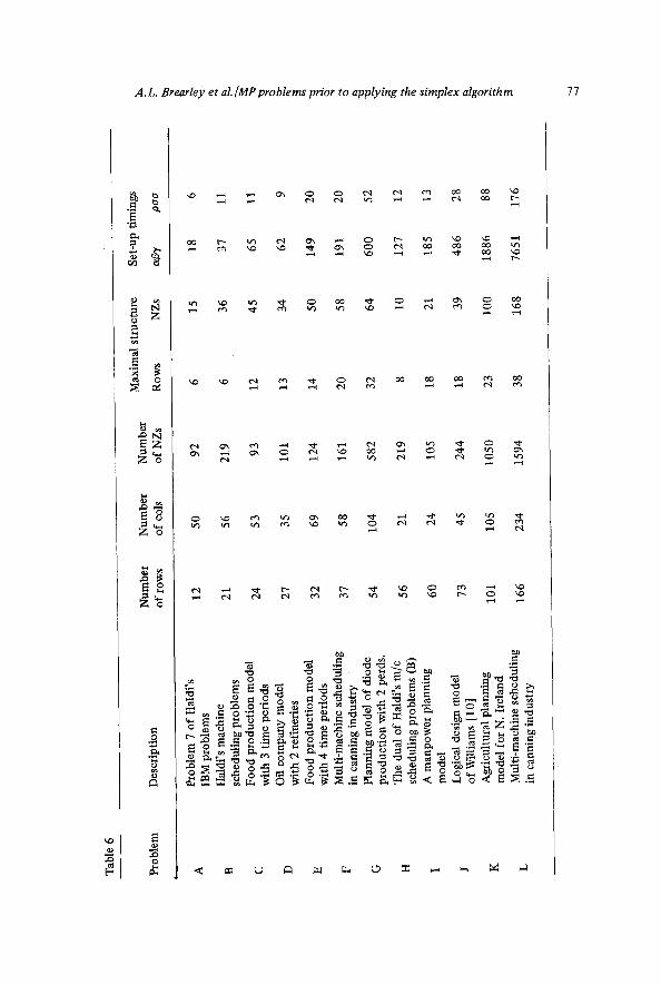
Method II.9 and II. 10 require the calculation of the vectors 0, a and v but this is straightforward and quick: for example, in the problem with 166 rows this set-up process took only 176 time units. All the methods considered have been incorporated in an ALGOL program for the ICL 4130 computer and have been applied to many linear and integer programming models. Their performances on twelve of these models is presented in Table 7(i) - 7(iii). The twelve models, which are described in Table 6, include three which are derived from Haldi [5] and nine which are based on real-life situations studied by the authors.

In Table 7 the numbers in the columns (a) are the numbers of rows in the structures identified by the methods, those in the columns (b) are the numbers of non-zero coefficients in the rows of those structures and the numbers in the columns (c) are the times taken to identify those structures. All timings are measured in internal t ime units.

Table 8 presents an analysis of the performance of the methods on the twelve problems. According to this analysis, the methods may be ranked into four groups by performance in identifying maximal structures:

(i) methods II.9 and II.10, which consistently perform very well, (ii) methods 1.2, 1.6, II.2 and II.6, all of which are related primarily

to the vector /3 and which perform almost as well as II.9 and II. 10,

(iii) methods 1.5, II.5, 1.7, II.7, I. 1 and II. 1, (iv) methods 1.3, II.3, 1.8, II.8, 1.4 and II.4, which per form quite

poorly.


02

o"1 ~ "~" O~ 0 O0 O0

7 8 A.L. BrearIey et al./MP problems prior to applying the simplex algorithm

ko

t o

,ff

o l

0

¢¢~¢q

eq oo

¢q oo

A.L. Brearley et al. IMP problems prior to applying the simplex algorithm 79

r¢1

t'q

e ~ ,

0

0 d~


~J

z

7~

C

A.L. Brearley e t al. IMP pro b le ms prior to apply ing the simplex algorithm

Table 8

81

Number of problems for which this row structure ...

1.1 1.2 1.3 1.4 1.5 1.6 1.7 1.8

is maximal 4 9 3 2 4 7 4 2

has as many rows as 4 1 1 0 .4 3 3 1 the maximal one has one fewer row

0 1 4 1 0 0 1 0 than the maximal one has two fewer ro~vs

2 1 0 1 2 2 2 2 than the maximal one

has at least as many 4 9 6 7 4 8 6 8 NZs as maximal one

Number of problems

for which the row II.1 II.2 II.3 I1.4 11.5 II.6 11.7 II.8 II.9 11.10 structure ...

is maximal 4 9 2 0 4 7 2 0 9 8 has as many rows as

4 0 0 0 4 3 3 1 2 3 the maximal one has one fewer row

0 2 3 1 0 0 2 1 1 0 than the maximal one has two fewer rows

2 1 0 2 2 2 3 2 0 1 than the maximal one has at least as many NZs as maximal one 4 11 11 10 4 8 6 8 9 8

Looking down each full column of Table 8, one observes that a selection heuristic performs just about as well or as badly in its Category II form as it does in its Category I form, thus tending to validate the assumption stated in Section 2.3. The analysis also indicates that methods using the un-updated versions of heuristics perform just about as well as those which use the updated versions; in some cases they appear ~o perform somewhat better, thus throwing up questions about the worth of those heuristics.

The timing figures for the methods on the twelve problems are of some considerable interest. Methods 1.5 to 1.8 are consistently faster than Methods I. 1 to 1.4 since they do not involve the updating of/31 and 3, I. However, this saving of time loses significance when the set-up time is included: for example, in the problem with 166 rows the difference between 425 and 578 time units is swamped by the overhead of 7651.

With Methods II. 1 to 11.8 the situation is more complex. Although the differences between methods is again insignificant compared with

8 2 A.L. Brearley et aL IMP problems prior to applying the simplex algorithm

the set-up overhead, in some cases the un-updated versions are faster then the updated versions and in others the opposite is true: for example, on problem I, updating appears to pay off whereas on problem J it does~not. Closer examination reveals that the expected computational advantage of Methods II.5 to II.8 is often offset by their need to make use of their second phases which require further set-ups: for example, Method II.2 uses its second phase on only three of the twelve problems whereas Method II.6 uses its second phase on all but three of the problems. Moreover, these methods tend to produce very small structures in their first phase by removing almost all the rows and then proceed to add many back into the structure in the second phase: for example, on problem G Method II.7 removes 53 of the 54 rows from the structure and then adds 19 of them back.

Methods II.9 and II. 10 differ considerably in their timings. Because of its need to re-compute the vector a n at each stage, Method II.9 is comparable with the fastest of the other sixteen methods. Method II. 10, however, is remarkably swift and would appear to be most worthy of further investigation.

Conclusions

The authors postulate that an analysis procedure should reduce problem dimension and find structure in LP problems so that the modified problem can be solved more efficiently than the original. Following this preliminary investigation, it is intended that much larger LP problems - up to 4000 rows - will be analysed using these algorithms. In these experiments the problems will be solved both before and after analysis in order to evaluate the usefulness of such a procedure.

Acknowledgment

The authors wish to thank Zvi Herzenshtein, Bill Morrison. John Luce and Colin Clayman, all of ICL/Dataskil, for their help and active interest in this project.

A.L. Brearley et aL /MP problems prior to applying the simplex algorithm 83

References

[1] APEX II, User Information Manual, 59158100 Rev. Control Data Corporation, Minnea- ~!is, U.S.A.

[2] E. Balas, "An additive algorithm for solving linear programs with zero-one variables", Operations Research, 13 (1965) 517-546.

[3] E.M.I. Beale, "Advanced algorithmic features for general mathematical programming systems", in: J. Abadie, ed., Integer and nonlinear programming (North Holland, Amsterdam, 1970) pp. 119-138.

[4] G.B. Dantzig and R.M. VanSlyke, "Generalized upper bounded techniques for linear programming", I, II, Operations Research Centre, University of California, Berkeley, CaliL, ORC 64-17, 18.

[5] J. Haldi, "25 integer programming test problems", Working Paper No. 43, Graduate School of Business, Stanford University, Stanford, Calif. (1964).

[6] A. Land and S. Powell, "FORTRAN codes for mathematical programming, linear, qua- dratic and discrete problems (Wiley, New York, 1973).

[7] Mathematical Programming System Extended (MPSX), Program Number 5734 XM4, IBM Trade Corporation, New York (1971).

[8] G. Mitra, "A generalized row elimination algorithm for exclusive row structure problems", ICL/DATASKIL Internal Rept. (1972).

[9] S. Senju and Y. Toyoda, "An approach to linear programming with 0-1 variables", Management Science (4) (1968) B196-B207.

[10] H.P. Williams, "Experiments in the formulation of integer programming problems", to appear.

[11 ] F.P. Wyman, "Binary programming: a decision rule for selecting optimal vs heuristic techniques", Computer Journal 16 (2) (1973) 135-140.

[12] G. Zoutendijk, "A product form algorithm using contracted transformation vectors,, in: J. Abadie, ed., Integer and nonlinear programming (North-Holland, Amsterdam, 1970) pp. 511-523.

Documents

Analysis of mathematical programming problems prior to ... · tected after solution has been attempted using the simplex method but often ... If qr < ql, replace qt by q}. If qr