Analysis of Head Losses in a Turbine Draft Tube by Means

HAL Id: hal-01418777https://hal.archives-ouvertes.fr/hal-01418777

Submitted on 17 Apr 2019

HAL is a multi-disciplinary open accessarchive for the deposit and dissemination of sci-entific research documents, whether they are pub-lished or not. The documents may come fromteaching and research institutions in France orabroad, or from public or private research centers.

L’archive ouverte pluridisciplinaire HAL, estdestinée au dépôt et à la diffusion de documentsscientifiques de niveau recherche, publiés ou non,émanant des établissements d’enseignement et derecherche français ou étrangers, des laboratoirespublics ou privés.

Analysis of Head Losses in a Turbine Draft Tube byMeans of 3D Unsteady Simulations

Sylvia Wilhelm, Guillaume Balarac, Olivier Métais, Claire Ségoufin

To cite this version:Sylvia Wilhelm, Guillaume Balarac, Olivier Métais, Claire Ségoufin. Analysis of Head Losses ina Turbine Draft Tube by Means of 3D Unsteady Simulations. Flow, Turbulence and Combustion,Springer Verlag (Germany), 2016, 97 (4), pp.1255-1280. �10.1007/s10494-016-9767-9�. �hal-01418777�

https://hal.archives-ouvertes.fr/hal-01418777

https://hal.archives-ouvertes.fr

Noname manuscript No.(will be inserted by the editor)

Analysis of head losses in a turbine draft tube by

means of 3D unsteady simulations

Sylvia Wilhelm · Guillaume Balarac ·Olivier Metais · Claire Segoufin

Received: date / Accepted: date

Abstract In this paper, Unsteady RANS (URANS) simulations and Large EddySimulations (LES) in the draft tube of a bulb turbine are presented with the ob-jective to understand and locate the head losses in this turbine component. Threeoperating points of the turbine are considered. Numerical results are compared withexperimental velocity measurements for validation. Thanks to a detailed analysis ofthe energy balance in the draft tube, the physical and hydrodynamic phenomenaresponsible for head losses in the draft tube are identified. Head losses are due totransfer of mean kinetic energy to the turbulent flow and viscous dissipation of ki-netic energy. This occurs mainly in the central vortex structure and next to the wallsin the draft tube. Head losses prediction is found to be dependent on the turbulencemodel used in the simulations, especially in URANS simulations. Using this analysis,the evolution of head losses between the three operating points is understood.

Keywords Unsteady RANS · Large Eddy Simulation · turbulence · hydraulicturbine · draft tube · head losses

1 Introduction

Hydroelectric energy production by exploitation of low head sites is an attractivealternative to the increase of energy demand. Bulb turbines constitute the mostefficient solution for low head sites thanks to their horizontal axis which enables lowconstruction costs and high performances [1]. Moreover, large operating ranges areensured by these double regulated turbines: guide vanes and blades angles are bothvarying in order to reach optimal performances.

The performances of low head turbines are highly influenced by the head losses inthe draft tube. The draft tube has a divergent shape in order to convert the residualkinetic energy leaving the runner into pressure and thus increase the effective head

S. Wilhelm · G. Balarac · O.MetaisGrenoble-INP/CNRS/UJF-Grenoble 1, LEGI UMR 5519, Grenoble, F-38041, FranceE-mail: [email protected]

C. SegoufinGE Renewable Energy, Hydro, 82 avenue Leon Blum, Grenoble, 38041, France

2 Sylvia Wilhelm et al.

of the turbine [2]. For low head turbines, the flow in the draft tube can lead to highenergy losses in comparison with other turbine components. The prediction of headlosses in the draft tube of bulb turbines is thereby a major issue. This can be done bymeans of experiments on test platform or by means of numerical simulation which isless expensive, more flexible and leads to a more complete database on the flow field.A better understanding of the flow phenomena occurring in the draft tube couldthus be achieved with high fidelity numerical simulations. However, the complexityof the flow in the draft tube (highly turbulent, swirling and decelerating) renders thenumerical prediction of the head losses very challenging.

In industry, steady RANS simulations of the draft tube flow using two equationslinear eddy-viscosity turbulence models are usually used due to their affordable com-putational cost. These models are robust, but the steady RANS approach is unable,by construction, to predict the unsteady flow in the draft tube [3]. Even with Un-steady RANS (URANS) simulations, unsteadiness and turbulent flow structures aredamped out when linear eddy-viscosity turbulence models are used [4,5]. Moreover,two equations turbulence models are not able to correctly account for turbulent pro-duction due to streamline curvature in swirling flows [6]. Corrections of these models,such as curvature correction [6,7] or turbulent production limiter [8], can be used toimprove the prediction of swirling flows in draft tubes [9]. Moreover, advanced RANSmodels such as Reynolds-stress-transport models, algebraic Reynolds-stress models,and non-linear eddy-viscosity models can lead to a better prediction of swirling flowssince they are more sensitive to flow instabilities and unsteadiness. However, whenusing statistical approaches, the turbulent part of the flow field is always modelledand only the large mean scales of the flow are explicitly solved. A better under-standing of the physic of highly turbulent flows in draft tubes can be obtained withimproved turbulence models such as Scale Adaptive Simulations (SAS), Zonal LargeEddy Simulations (ZLES) or Hybrid RANS-LES turbulence models such as DetachedEddy Simulations (DES) [10,4,11,12]. In particular, DES in a Francis turbine drafttube were performed in [4,11,12] which led to a more complete physical descriptionof the flow than with URANS simulations. However, head losses prediction was notimproved with DES simulations. Therefore an improvement of the flow predictioncan be expected with LES which could capture the complex, 3D phenomena devel-oping in the draft tube, but with a much higher computational cost than for classicRANS calculations [13]. Moreover, the authors of [11–13] point out that accurateinlet boundary conditions accounting for the unsteadiness from the runner are nec-essary to improve the flow prediction in the draft tube. The strong sensitivity to inletvelocity profiles prescription on the flow prediction in the draft tube of axial tur-bines has indeed been observed in several studies [14–18]. In particular, an accuratedescription of the flow from the hub and shroud gaps is necessary [19,20].

The objective of this paper is to perform a precise analysis of the highly tur-bulent flow in the draft tube of a bulb turbine in order to better understand theflow phenomena leading to head losses in this component. Both Unsteady RANS(URANS) calculations and Large Eddy Simulations (LES) are used for this purposeand their reliability is evaluated through comparisons with experimental data. Aspreviously pointed out, numerous URANS modelling approaches have been devel-oped but we here restrict our study to URANS based on the k − ω SST turbulencemodel [21] since it is the most widely used in hydraulic machinery industry for itsrecognized performances [22,9,17]. In these numerical simulations, unsteady inletboundary conditions are used to take into account the unsteady phenomena coming

Numerical analysis of head losses in draft tube 3

from the runner. From these simulations, a local analysis of the predicted flow fieldusing the energy balance in the draft tube is performed to understand the main phys-ical phenomena responsible for head losses. Three operating points are considered:the best efficiency point of the turbine, leading to the lowest head losses, and twooff-design points.

2 Methodology

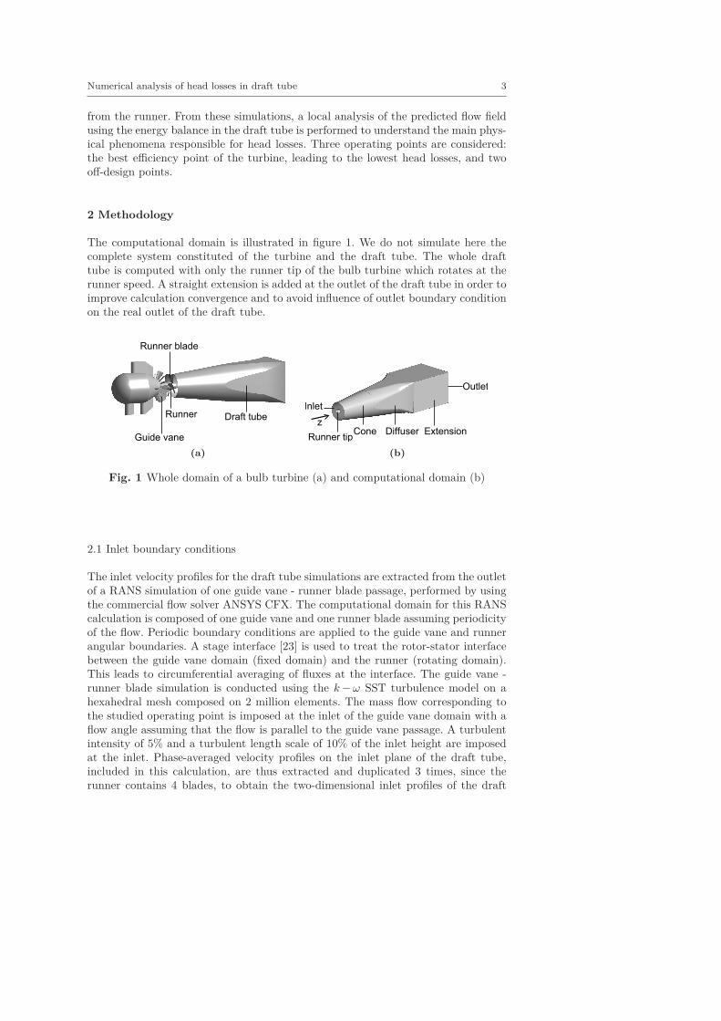
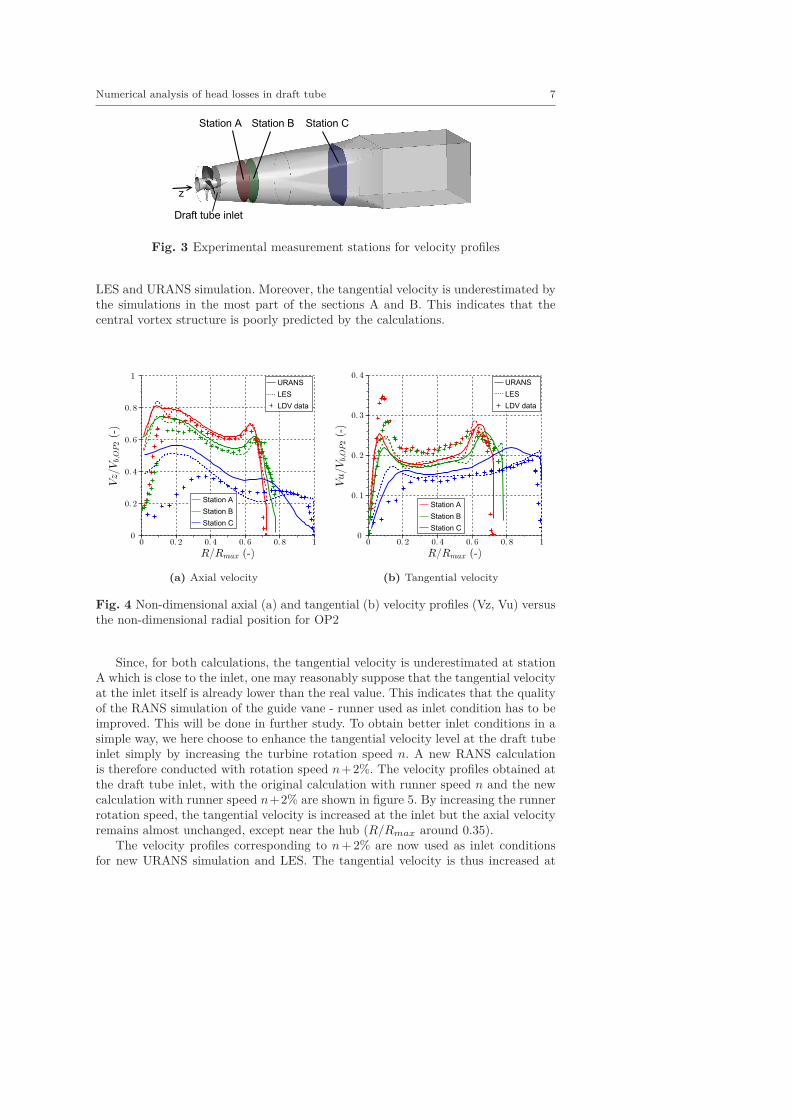
The computational domain is illustrated in figure 1. We do not simulate here thecomplete system constituted of the turbine and the draft tube. The whole drafttube is computed with only the runner tip of the bulb turbine which rotates at therunner speed. A straight extension is added at the outlet of the draft tube in order toimprove calculation convergence and to avoid influence of outlet boundary conditionon the real outlet of the draft tube.

Guide vane

Runner Draft tube

Runner blade

(a)

Runner tipCone Diffuser Extension

Inlet

Outlet

z

(b)

Fig. 1 Whole domain of a bulb turbine (a) and computational domain (b)

2.1 Inlet boundary conditions

The inlet velocity profiles for the draft tube simulations are extracted from the outletof a RANS simulation of one guide vane - runner blade passage, performed by usingthe commercial flow solver ANSYS CFX. The computational domain for this RANScalculation is composed of one guide vane and one runner blade assuming periodicityof the flow. Periodic boundary conditions are applied to the guide vane and runnerangular boundaries. A stage interface [23] is used to treat the rotor-stator interfacebetween the guide vane domain (fixed domain) and the runner (rotating domain).This leads to circumferential averaging of fluxes at the interface. The guide vane -runner blade simulation is conducted using the k − ω SST turbulence model on ahexahedral mesh composed on 2 million elements. The mass flow corresponding tothe studied operating point is imposed at the inlet of the guide vane domain with aflow angle assuming that the flow is parallel to the guide vane passage. A turbulentintensity of 5% and a turbulent length scale of 10% of the inlet height are imposedat the inlet. Phase-averaged velocity profiles on the inlet plane of the draft tube,included in this calculation, are thus extracted and duplicated 3 times, since therunner contains 4 blades, to obtain the two-dimensional inlet profiles of the draft


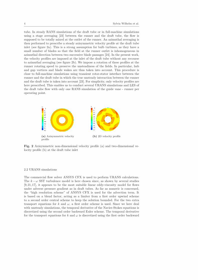
tube. In steady RANS simulations of the draft tube or in full-machine simulationsusing a stage averaging [23] between the runner and the draft tube, the flow issupposed to be totally mixed at the outlet of the runner. An azimuthal averaging isthen performed to prescribe a steady axisymmetric velocity profile at the draft tubeinlet (see figure 2a). This is a strong assumption for bulb turbines, as they have asmall number of blades so that the field at the runner outlet is inhomogeneous inazimuthal direction between two successive blade passages [24]. In the present work,the velocity profiles are imposed at the inlet of the draft tube without any recourseto azimuthal averaging (see figure 2b). We impose a rotation of these profiles at therunner rotating speed to preserve the unsteadiness of the fields. In particular, huband gap vortices and blade wakes are thus taken into account. This procedure isclose to full-machine simulations using transient rotor-stator interface between therunner and the draft tube in which the true unsteady interaction between the runnerand the draft tube is taken into account [23]. For simplicity, only velocity profiles arehere prescribed. This enables us to conduct several URANS simulations and LES ofthe draft tube flow with only one RANS simulation of the guide vane - runner peroperating point.

(a) Axisymmetric velocityprofile

(b) 2D velocity profile

Fig. 2 Axisymmetric non-dimensional velocity profile (a) and two-dimensional ve-locity profile (b) at the draft tube inlet

2.2 URANS simulations

The commercial flow solver ANSYS CFX is used to perform URANS calculations.The k − ω SST turbulence model is here chosen since, as shown by several studies[9,21,17], it appears to be the most suitable linear eddy-viscosity model for flowsunder adverse pressure gradient as in draft tubes. As far as numeric is concerned,the “high resolution scheme” of ANSYS CFX is used for the advection term. Itis based on a blend factor, acting as a limiter from a first order upwind schemeto a second order central scheme to keep the solution bounded. For the two extratransport equations for k and ω, a first order scheme is used. Since we here dealwith unsteady simulations, the temporal derivative of the Navier-Stokes equations isdiscretized using the second order backward Euler scheme. The temporal derivativefor the transport equations for k and ω is discretized using the first order backward


Euler scheme. In k − ω SST URANS simulations, the prescription at the inlet ofturbulence quantities is necessary to be able to resolve the transport equations fork and ω. In steady RANS simulations, uniform turbulent quantities are usuallyimposed according to best practice guidelines [17]. In the present work, k and ωprofiles are extracted from the guide vane - runner RANS simulation and imposed atthe draft tube inlet similarly as for velocity profiles (see section 2.1). The averagedstatic pressure at the outlet is imposed equal to 0. No-slip condition is imposed onthe stationary walls. The runner tip is a rotating wall with a velocity equal therunner rotation speed. Note that we have verified that these inlet conditions lead tothe same results a fully coupled simulation including guide vane, runner and drafttube with transient rotor-stator interface between the runner and the draft tube.This indicates that the flow in the draft tube has very little influence on the runnerflow field and both calculations can therefore be decoupled.

The block-structured hexahedral mesh for the draft tube is composed on 2 millionelements (including the extension). The size of the first cells close to the wall in wallunits, y+, has a mean value of 5 and varies from 10 on the runner tip to 0.1 inthe extension. A logarithmic wall function is used in CFX [25]. Mesh convergencehas been checked for the draft tube to assess the independence of the results (seeappendix A.1).

Convergence tests lead to a time step corresponding to five degrees of runnerrotation per time step. The transient part of the simulations is performed for ap-proximately four flow passages through the draft tube. Flow statistics are calculatedon a time length corresponding to two flow passages through the draft tube whichproved to be sufficient for statistical convergence. This methodology is an improve-ment of the classical RANS simulations of the draft tube because of the unsteadinessof the computation but also thanks to an improved description of the inlet velocityprofiles.

2.3 Large Eddy Simulations (LES)

LES computations are carried out with the YALES2 incompressible fractional-stepsolver with a finite-volume formulation with numerical schemes of 4th order in timeand space [26]. The dynamic Smagorinsky subgrid-scale model is used [27].

No turbulence is imposed at the inlet. In this swirling flow, the instabilities arefound to develop without the addition of inflow perturbations. As for the URANScomputations, a rotating wall at the runner speed is imposed for the runner tip.No-slip condition is imposed on the walls.

The mesh is composed of tetrahedral elements with prisms layers at the wall inorder to ensure a small value of y+ with a reasonable number of elements. A meshcomposed of 16 million elements with a y+ ranging from 10 to 20 is generated. Anal-ysis on the near-wall mesh resolution and on the discretization of the internal flowhave shown that this resolution is enough for the flow prediction in the draft tube(see appendix A.2). The time step complies with the CFL condition and correspondsto around 0.07 degree of runner rotation. The simulation is run until quantities ofinterest are converged (head losses, velocity profiles). This transient stage needs be-tween two and four flow passages through the draft tube, depending on the operatingpoints. Flow statistics are then calculated. The statistics are computed on a periodcorresponding to four flow passages through the draft tube.


3 Flow prediction in the draft tube

The flow field in the draft tube is calculated for three operating points of the bulbturbine, from low to high flow rate, with a constant blade angle. OP1 corresponds tothe off-design point at partial load (low flow rate). OP2 corresponds to the optimalpoint, where the efficiency of the turbine is the highest. OP3 corresponds to thepoint at high load (high flow rate). Table 1 gives the non-dimensional parametersfor each operating point. The Reynolds number is defined with the bulk velocity andthe maximum radius on the inlet section. The Swirl number is defined as,

S = 1

R2−R1

∫

SVzVurdS

∫

SV 2

z dS

where Vz and Vu are respectively the axial and tangential velocity, r is the radius onthe inlet section and R1 and R2 are respectively the minimum and maximum radiusat the inlet section.

Table 1 Flow parameters for the considered operating points. Q is the flow rate, Reis the Reynolds number and S is the Swirl number.

Operating point Q/QOP 2 Re S

OP1 0.954 1.106 0.34OP2 1.000 2.4.106 0.23OP3 1.122 2.7.106

−0.4.10−3

3.1 Validation of the simulations for the best efficiency point OP2

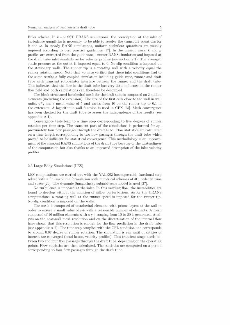
For the validation of the numerical simulations, experimental axial (Vz) and tan-gential (Vu) velocity profiles, measured by means of 2D-LDV (Laser Doppler Ve-locimetry), are used at three stations in the draft tube shown in figure 3: stationsA and B in the cone and station C in the diffuser. The axial velocity Vz is the ve-locity component along the z axis (see figure 3) and the tangential velocity Vu ispositive in the runner rotation direction. Note that velocities presented in this paperare dimensionless, obtained by dividing velocity values by the bulk velocity at OP2Vb,OP 2.

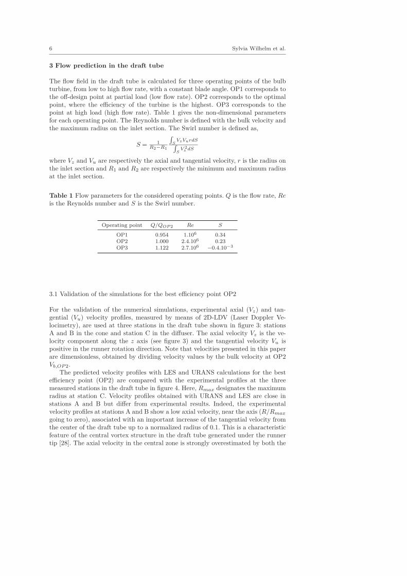
The predicted velocity profiles with LES and URANS calculations for the bestefficiency point (OP2) are compared with the experimental profiles at the threemeasured stations in the draft tube in figure 4. Here, Rmax designates the maximumradius at station C. Velocity profiles obtained with URANS and LES are close instations A and B but differ from experimental results. Indeed, the experimentalvelocity profiles at stations A and B show a low axial velocity, near the axis (R/Rmax

going to zero), associated with an important increase of the tangential velocity fromthe center of the draft tube up to a normalized radius of 0.1. This is a characteristicfeature of the central vortex structure in the draft tube generated under the runnertip [28]. The axial velocity in the central zone is strongly overestimated by both the


Station A Station B Station C

Draft tube inlet

z

Fig. 3 Experimental measurement stations for velocity profiles

LES and URANS simulation. Moreover, the tangential velocity is underestimated bythe simulations in the most part of the sections A and B. This indicates that thecentral vortex structure is poorly predicted by the calculations.

URANS

LES

LDV data

Station A

Station B

Station C

(a) Axial velocity

URANS

LES

LDV data

Station A

Station B

Station C

(b) Tangential velocity

Fig. 4 Non-dimensional axial (a) and tangential (b) velocity profiles (Vz, Vu) versusthe non-dimensional radial position for OP2

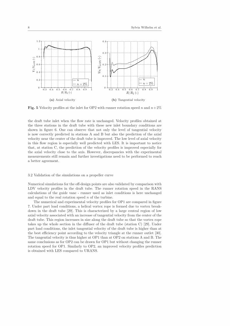
Since, for both calculations, the tangential velocity is underestimated at stationA which is close to the inlet, one may reasonably suppose that the tangential velocityat the inlet itself is already lower than the real value. This indicates that the qualityof the RANS simulation of the guide vane - runner used as inlet condition has to beimproved. This will be done in further study. To obtain better inlet conditions in asimple way, we here choose to enhance the tangential velocity level at the draft tubeinlet simply by increasing the turbine rotation speed n. A new RANS calculationis therefore conducted with rotation speed n+2%. The velocity profiles obtained atthe draft tube inlet, with the original calculation with runner speed n and the newcalculation with runner speed n+2% are shown in figure 5. By increasing the runnerrotation speed, the tangential velocity is increased at the inlet but the axial velocityremains almost unchanged, except near the hub (R/Rmax around 0.35).

The velocity profiles corresponding to n + 2% are now used as inlet conditionsfor new URANS simulation and LES. The tangential velocity is thus increased at


(a) Axial velocity (b) Tangential velocity

Fig. 5 Velocity profiles at the inlet for OP2 with runner rotation speed n and n+2%

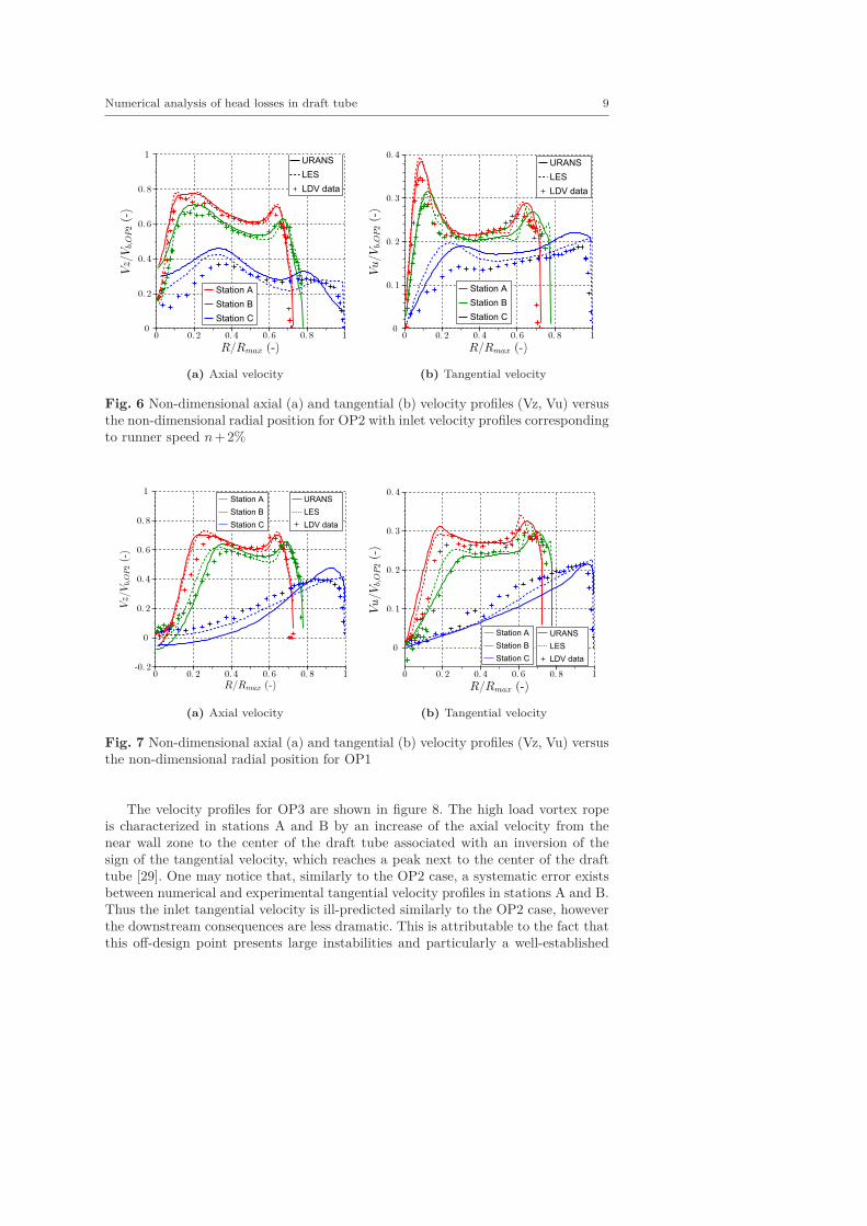
the draft tube inlet when the flow rate is unchanged. Velocity profiles obtained atthe three stations in the draft tube with these new inlet boundary conditions areshown in figure 6. One can observe that not only the level of tangential velocityis now correctly predicted in stations A and B but also the prediction of the axialvelocity near the center of the draft tube is improved. The low level of axial velocityin this flow region is especially well predicted with LES. It is important to noticethat, at station C, the prediction of the velocity profiles is improved especially forthe axial velocity close to the axis. However, discrepancies with the experimentalmeasurements still remain and further investigations need to be performed to reacha better agreement.

3.2 Validation of the simulations on a propeller curve

Numerical simulations for the off-design points are also validated by comparison withLDV velocity profiles in the draft tube. The runner rotation speed in the RANScalculations of the guide vane - runner used as inlet conditions is here unchangedand equal to the real rotation speed n of the turbine.

The numerical and experimental velocity profiles for OP1 are compared in figure7. Under part load conditions, a helical vortex rope is formed due to vortex break-down in the draft tube [29]. This is characterized by a large central region of lowaxial velocity associated with an increase of tangential velocity from the center of thedraft tube. This region increases in size along the draft tube so that the vortex ropetakes up the whole section in the diffuser of the draft tube (station C) [29]. Underpart load conditions, the inlet tangential velocity of the draft tube is higher than atthe best efficiency point according to the velocity triangle at the runner outlet [30].The tangential velocity is thus higher at OP1 than at OP2 on stations A and B. Thesame conclusions as for OP2 can be drawn for OP1 but without changing the runnerrotation speed for OP1. Similarly to OP2, an improved velocity profiles predictionis obtained with LES compared to URANS.


URANS

LES

LDV data

Station A

Station B

Station C

(a) Axial velocity

URANS

LES

LDV data

Station A

Station B

Station C


Fig. 6 Non-dimensional axial (a) and tangential (b) velocity profiles (Vz, Vu) versusthe non-dimensional radial position for OP2 with inlet velocity profiles correspondingto runner speed n+2%

URANS

LES

LDV data

Station A

Station B

Station C

(a) Axial velocity

URANS

LES

LDV data

Station A

Station B

Station C



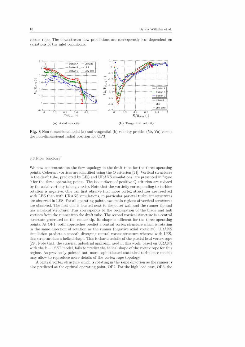
The velocity profiles for OP3 are shown in figure 8. The high load vortex ropeis characterized in stations A and B by an increase of the axial velocity from thenear wall zone to the center of the draft tube associated with an inversion of thesign of the tangential velocity, which reaches a peak next to the center of the drafttube [29]. One may notice that, similarly to the OP2 case, a systematic error existsbetween numerical and experimental tangential velocity profiles in stations A and B.Thus the inlet tangential velocity is ill-predicted similarly to the OP2 case, howeverthe downstream consequences are less dramatic. This is attributable to the fact thatthis off-design point presents large instabilities and particularly a well-established


vortex rope. The downstream flow predictions are consequently less dependent onvariations of the inlet conditions.

URANS

LES

LDV data

Station A

Station B

Station C

(a) Axial velocity

URANS

LES

LDV data

Station A

Station B

Station C



3.3 Flow topology

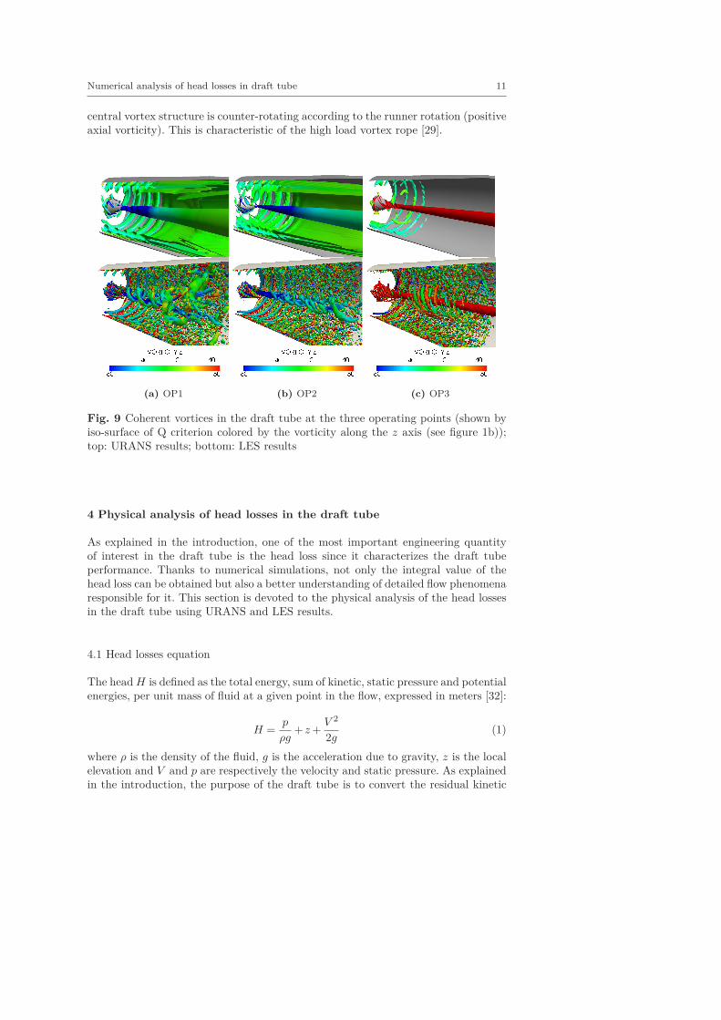
We now concentrate on the flow topology in the draft tube for the three operatingpoints. Coherent vortices are identified using the Q criterion [31]. Vortical structuresin the draft tube, predicted by LES and URANS simulations, are presented in figure9 for the three operating points. The iso-surfaces of positive Q criterion are coloredby the axial vorticity (along z axis). Note that the vorticity corresponding to turbinerotation is negative. One can first observe that more vortex structures are resolvedwith LES than with URANS simulations, in particular parietal turbulent structuresare observed in LES. For all operating points, two main regions of vortical structuresare observed. The first one is located next to the outer wall and the runner tip andhas a helical structure. This corresponds to the propagation of the blade and hubvortices from the runner into the draft tube. The second vortical structure is a centralstructure generated on the runner tip. Its shape is different for the three operatingpoints. At OP1, both approaches predict a central vortex structure which is rotatingin the same direction of rotation as the runner (negative axial vorticity). URANSsimulation predicts a smooth diverging central vortex structure whereas with LES,this structure has a helical shape. This is characteristic of the partial load vortex rope[29]. Note that, the classical industrial approach used in this work, based on URANSwith the k−ω SST model, fails to predict the helical shape of the vortex rope for thisregime. As previously pointed out, more sophisticated statistical turbulence modelsmay allow to reproduce more details of the vortex rope topology.

A central vortex structure which is rotating in the same direction as the runner isalso predicted at the optimal operating point, OP2. For the high load case, OP3, the


central vortex structure is counter-rotating according to the runner rotation (positiveaxial vorticity). This is characteristic of the high load vortex rope [29].

(a) OP1 (b) OP2 (c) OP3

Fig. 9 Coherent vortices in the draft tube at the three operating points (shown byiso-surface of Q criterion colored by the vorticity along the z axis (see figure 1b));top: URANS results; bottom: LES results

4 Physical analysis of head losses in the draft tube

As explained in the introduction, one of the most important engineering quantityof interest in the draft tube is the head loss since it characterizes the draft tubeperformance. Thanks to numerical simulations, not only the integral value of thehead loss can be obtained but also a better understanding of detailed flow phenomenaresponsible for it. This section is devoted to the physical analysis of the head lossesin the draft tube using URANS and LES results.

4.1 Head losses equation

The head H is defined as the total energy, sum of kinetic, static pressure and potentialenergies, per unit mass of fluid at a given point in the flow, expressed in meters [32]:

H =p

ρg+z +

V 2

2g(1)

where ρ is the density of the fluid, g is the acceleration due to gravity, z is the localelevation and V and p are respectively the velocity and static pressure. As explainedin the introduction, the purpose of the draft tube is to convert the residual kinetic


energy at the runner outlet into static pressure. Hence, the head losses in the drafttube correspond to the total energy loss due to the kinetic energy which is notconverted into static pressure but into heat through viscous dissipation.

The flow in the draft tube is governed by the Navier-Stokes equations for anincompressible turbulent flow. The equation for the mean kinetic energy can bederived from Navier-Stokes equations and leads to the following equation (note thatthe operator 〈a〉 corresponds to the time averaged value of a obtained from flowstatistics):

∂

∂xj

(〈p〉

ρg+z +

1

2g〈ui〉〈ui〉

)

g〈uj〉

= 2ν∂

∂xj(〈ui〉〈Sij〉)

︸︷︷︸

I

−∂

∂xj

(〈ui〉〈u

′

iu′

j〉)

︸︷︷︸

II

−2ν〈Sij〉〈Sij〉︸︷︷︸

III

+〈u′

iu′

j〉〈Sij〉︸︷︷︸

IV

(2)

where ν is the fluid kinematic viscosity, ui is the velocity in xi direction with

ui = 〈ui〉 + u′

i, and Sij = 1

2

(∂ui∂xj

+∂uj

∂xi

)

is strain rate tensor. Terms (I) and (II)

correspond to diffusion of mean kinetic energy. Term (III) corresponds to the vis-cous dissipation of mean kinetic energy. Term (IV ) is responsible for the transfer ofmean kinetic energy to the turbulent kinetic energy i.e. for turbulent kinetic energyproduction. This turbulent kinetic energy is then dissipated by the small scales ofturbulence through viscous dissipation [33].

Since the total head loss in the draft tube corresponds to an integral value, equa-tion (2) has to be integrated over the total volume V of the draft tube. Lets designateby S its external surface and by nj the jth component of the outer-pointing normal.By using the divergence theorem, the energy balance in the draft tube becomes :

∫∫

S

(〈p〉

ρg+z +

1

2g〈ui〉〈ui〉

)

g〈uj〉njdS

= 2ν

∫∫

S

(〈ui〉〈Sij〉)njdS −

∫∫

S

(〈ui〉〈u

′

iu′

j〉)

njdS

−2ν

∫∫∫

V

〈Sij〉〈Sij〉dV +

∫∫∫

V

〈u′

iu′

j〉〈Sij〉dV

(3)

On the left-hand side of equation (3), one can recognize the head flux through thedraft tube external surface. This flux is obviously zero through the lateral solidsurfaces which are impermeable. The assumption of a steady flow with constant flowrate Q and uniform head H on the inlet (suffix in) and outlet (suffix out) surfacesof the draft tube then leads to:

∫∫

Sin

(〈p〉

ρg+z +

1

2g〈ui〉〈ui〉

)

g〈uz〉dS −

∫∫

Sout

(〈p〉

ρg+z +

1

2g〈ui〉〈ui〉

)

g〈uz〉dS

= gQ(Hin −Hout)

(4)

One thus obtains the expression for the total head loss ∆H = Hin −Hout.


Physical phenomena responsible for head losses

According to equations (3) and (4), the head losses in the draft tube are influencedby four terms :

gQ∆H = −2ν

∫∫

S

(〈ui〉〈Sij〉)njdS

︸︷︷︸

I

+

∫∫

S

(〈ui〉〈u

′

iu′

j〉)

njdS

︸︷︷︸

II

+2ν

∫∫∫

V

〈Sij〉〈Sij〉dV

︸︷︷︸

III

+

∫∫∫

V

−〈u′

iu′

j〉〈Sij〉dV

︸︷︷︸

IV

(5)

On the right-hand side of equation (5), terms (I) and (II) correspond to the diffusionof mean kinetic energy. Terms (III) and (IV ) contribute to head losses by viscousdissipation of the mean kinetic energy either directly by the mean flow or indirectlyafter turbulent kinetic energy production.

4.2 Turbulence modelling and head losses prediction

In LES and URANS simulations, only filtered and mean values (according to theReynolds decomposition) of pressure and velocity are respectively resolved and tur-bulence modelling is used to take into account the effect of the unresolved part ofthe flow on the resolved one. Lets designate by a the mean value of a in case of aURANS calculation and the filtered value of a in the LES case. Equation (5) thenyields:

gQ∆H =∫∫

Sin

(〈P∗〉

ρg+

1

2g〈ui〉〈ui〉

)

g〈uz〉dS −

∫∫

Sout

(〈P∗〉

ρg+

1

2g〈ui〉〈ui〉

)

g〈uz〉dS

= −

∫∫

S

(2〈ui〉(ν〈Sij〉+ 〈νtSij〉)nj

)dS

︸︷︷︸

I

+

∫∫

S

〈ui〉〈ui′uj

′〉njdS

︸︷︷︸

II

+

∫∫∫

V

2ν〈Sij〉〈Sij〉dV

︸︷︷︸

III

+

∫∫∫

V

−〈ui′uj

′〉〈Sij〉dV

︸︷︷︸

IV

+

∫∫∫

V

2〈νtSij〉〈Sij〉dV

︸︷︷︸

V

(6)

where 〈P∗〉 is the modified pressure. νt corresponds to the turbulent viscosity inthe case of a URANS calculation or to the eddy viscosity in the case of LES. Weconcentrate on the different terms of the right-hand side of equation (6). The termsinvolving the viscosity νt are dependent on the model used for the simulation: k −ωSST model for the URANS calculations and the dynamic Smagorinsky model forthe LES. Terms (I) and (II) correspond to the diffusion of mean kinetic energy andterm (III) is the viscous dissipation of mean kinetic energy. The turbulent kinetic


energy production decomposes into a (IV ) resolved and a (V ) modelled part whichinvolves the turbulent viscosity νt.

Two levels of analysis of head losses are performed in this work. An overallanalysis is first conducted which consists of calculating the different terms of equation(6) in order to determine the leading terms responsible for the head losses. A localanalysis is then performed to investigate the spatial distribution of these leadingterms within the draft tube. Similar analysis has been performed experimentally in[34] and numerically in [35] in order to study energy losses in a turbine cascade.It was concluded that the viscous dissipation of turbulent kinetic energy producedfrom the mean flow predominates in total pressure losses generation.

Best efficiency point OP2

The terms of equation (6) have been calculated both for LES and URANS compu-tations for all operating points. The conclusions are similar for the three operatingpoints and are only shown for the best efficiency point, OP2. It is important tocheck the ability for the numerics to accurately reproduce the balance between theleft hand side and the right hand side of equation (6). We have observed that theURANS leads to a difference of 4.8% when it is only of 0.02% for the LES.

Surface integrals in equation (6) are found to be negligible in front of vol-ume integrals in the energy balance. We note PM =

∫∫∫

V

2〈νtSij〉〈Sij〉dV and PR =

∫∫∫

V

−〈ui′uj

′〉〈Sij〉dV the two parts of the turbulent kinetic energy production which

are respectively modelled and resolved. D =∫∫∫

V

2ν〈Sij〉〈Sij〉dV is the viscous dis-

sipation of the mean kinetic energy. Note that the viscous dissipation by the smallscales of turbulence does not appear explicitly but implicitly through PM .

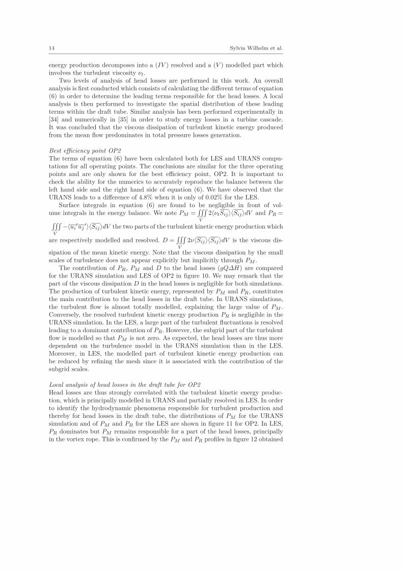
The contribution of PR, PM and D to the head losses (gQ∆H) are comparedfor the URANS simulation and LES of OP2 in figure 10. We may remark that thepart of the viscous dissipation D in the head losses is negligible for both simulations.The production of turbulent kinetic energy, represented by PM and PR, constitutesthe main contribution to the head losses in the draft tube. In URANS simulations,the turbulent flow is almost totally modelled, explaining the large value of PM .Conversely, the resolved turbulent kinetic energy production PR is negligible in theURANS simulation. In the LES, a large part of the turbulent fluctuations is resolvedleading to a dominant contribution of PR. However, the subgrid part of the turbulentflow is modelled so that PM is not zero. As expected, the head losses are thus moredependent on the turbulence model in the URANS simulation than in the LES.Moreover, in LES, the modelled part of turbulent kinetic energy production canbe reduced by refining the mesh since it is associated with the contribution of thesubgrid scales.

Local analysis of head losses in the draft tube for OP2

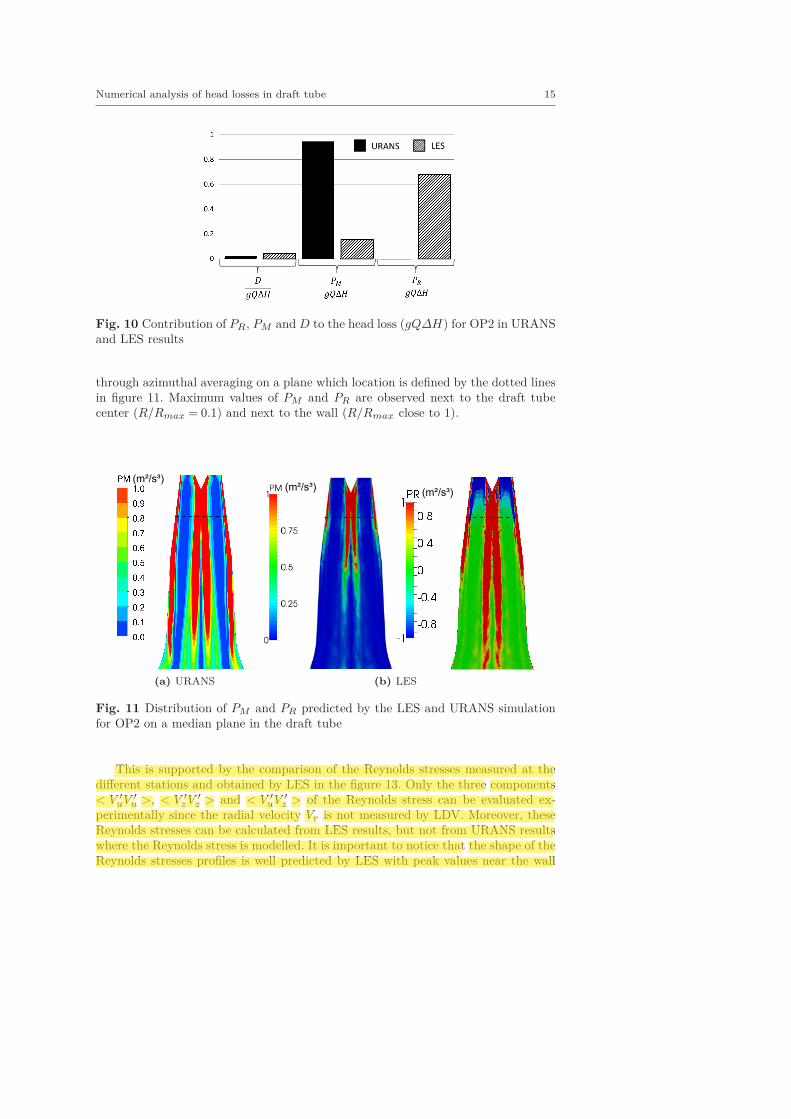
Head losses are thus strongly correlated with the turbulent kinetic energy produc-tion, which is principally modelled in URANS and partially resolved in LES. In orderto identify the hydrodynamic phenomena responsible for turbulent production andthereby for head losses in the draft tube, the distributions of PM for the URANSsimulation and of PM and PR for the LES are shown in figure 11 for OP2. In LES,PR dominates but PM remains responsible for a part of the head losses, principallyin the vortex rope. This is confirmed by the PM and PR profiles in figure 12 obtained


Fig. 10 Contribution of PR, PM and D to the head loss (gQ∆H) for OP2 in URANSand LES results

through azimuthal averaging on a plane which location is defined by the dotted linesin figure 11. Maximum values of PM and PR are observed next to the draft tubecenter (R/Rmax = 0.1) and next to the wall (R/Rmax close to 1).

(m²/s³)

(a) URANS

(m²/s³)(m²/s³)

(b) LES

Fig. 11 Distribution of PM and PR predicted by the LES and URANS simulationfor OP2 on a median plane in the draft tube

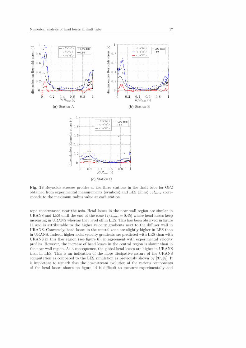
This is supported by the comparison of the Reynolds stresses measured at thedifferent stations and obtained by LES in the figure 13. Only the three components< V ′

uV ′

u >, < V ′

zV ′

z > and < V ′

uV ′

z > of the Reynolds stress can be evaluated ex-perimentally since the radial velocity Vr is not measured by LDV. Moreover, theseReynolds stresses can be calculated from LES results, but not from URANS resultswhere the Reynolds stress is modelled. It is important to notice that the shape of theReynolds stresses profiles is well predicted by LES with peak values near the wall

swilhelm

Highlight


URANS

LES

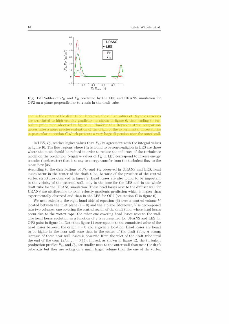
Fig. 12 Profiles of PM and PR predicted by the LES and URANS simulation forOP2 on a plane perpendicular to z axis in the draft tube

and in the center of the draft tube. Moreover, these high values of Reynolds stressesare associated to high velocity gradients, as shown in figure 6, thus leading to tur-bulent production observed in figure 11. However this Reynolds stress comparisonnecessitates a more precise evaluation of the origin of the experimental uncertaintiesin particular at section C which presents a very large dispersion near the outer wall.

In LES, PR reaches higher values than PM in agreement with the integral valuesin figure 10. The flow regions where PM is found to be non-negligible in LES are thosewhere the mesh should be refined in order to reduce the influence of the turbulencemodel on the prediction. Negative values of PR in LES correspond to inverse energytransfer (backscatter) that is to say to energy transfer from the turbulent flow to themean flow [36].According to the distributions of PM and PR observed in URANS and LES, headlosses occur in the center of the draft tube, because of the presence of the centralvortex structures observed in figure 9. Head losses are also found to be importantin the vicinity of the external wall, only in the cone for the LES and in the wholedraft tube for the URANS simulation. These head losses next to the diffuser wall forURANS are attributable to axial velocity gradients prediction which is higher thanexperimentally observed and than in the LES for OP2 (see station C in figure 6).

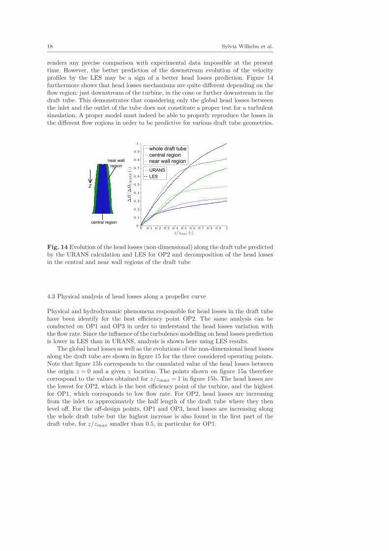
We next calculate the right-hand side of equation (6) over a control volume Vlocated between the inlet plane (z = 0) and the z plane. Moreover, V is decomposedinto two volumes: one covering the central region of the draft tube, where head lossesoccur due to the vortex rope, the other one covering head losses next to the wall.The head losses evolution as a function of z is represented for URANS and LES forOP2 point in figure 14. Note that figure 14 corresponds to the cumulated value of thehead losses between the origin z = 0 and a given z location. Head losses are foundto be higher in the near wall zone than in the center of the draft tube. A strongincrease of these near wall losses is observed from the inlet of the draft tube untilthe end of the cone (z/zmax = 0.45). Indeed, as shown in figure 12, the turbulentproduction profiles PM and PR are smaller next to the outer wall than near the drafttube axis but they are acting on a much larger volume than the one of the vortex

swilhelm

Highlight


LDV data

LES

(a) Station A

LDV data

LES

(b) Station B

LDV data

LES

(c) Station C

Fig. 13 Reynolds stresses profiles at the three stations in the draft tube for OP2obtained from experimental measurements (symbols) and LES (lines) ; Rmax corre-sponds to the maximum radius value at each station

rope concentrated near the axis. Head losses in the near wall region are similar inURANS and LES until the end of the cone (z/zmax = 0.45) where head losses keepincreasing in URANS whereas they level off in LES. This has been observed in figure11 and is attributable to the higher velocity gradients next to the diffuser wall inURANS. Conversely, head losses in the central zone are slightly higher in LES thanin URANS. Indeed, higher axial velocity gradients are predicted with LES than withURANS in this flow region (see figure 6), in agreement with experimental velocityprofiles. However, the increase of head losses in the central region is slower than inthe near wall region. As a consequence, the global head losses are higher in URANSthan in LES. This is an indication of the more dissipative nature of the URANScomputation as compared to the LES simulation as previously shown by [37,38]. Itis important to remark that the downstream evolution of the various componentsof the head losses shown on figure 14 is difficult to measure experimentally and


renders any precise comparison with experimental data impossible at the presenttime. However, the better prediction of the downstream evolution of the velocityprofiles by the LES may be a sign of a better head losses prediction. Figure 14furthermore shows that head losses mechanisms are quite different depending on theflow region: just downstream of the turbine, in the cone or further downstream in thedraft tube. This demonstrates that considering only the global head losses betweenthe inlet and the outlet of the tube does not constitute a proper test for a turbulentsimulation. A proper model must indeed be able to properly reproduce the losses inthe different flow regions in order to be predictive for various draft tube geometries.

central region

near wall

region

Z

URANS

LES

central region

near wall region

whole draft tube

Fig. 14 Evolution of the head losses (non-dimensional) along the draft tube predictedby the URANS calculation and LES for OP2 and decomposition of the head lossesin the central and near wall regions of the draft tube

4.3 Physical analysis of head losses along a propeller curve

Physical and hydrodynamic phenomena responsible for head losses in the draft tubehave been identify for the best efficiency point OP2. The same analysis can beconducted on OP1 and OP3 in order to understand the head losses variation withthe flow rate. Since the influence of the turbulence modelling on head losses predictionis lower in LES than in URANS, analysis is shown here using LES results.

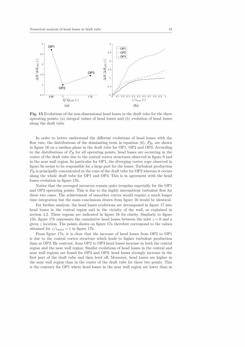
The global head losses as well as the evolutions of the non-dimensional head lossesalong the draft tube are shown in figure 15 for the three considered operating points.Note that figure 15b corresponds to the cumulated value of the head losses betweenthe origin z = 0 and a given z location. The points shown on figure 15a thereforecorrespond to the values obtained for z/zmax = 1 in figure 15b. The head losses arethe lowest for OP2, which is the best efficiency point of the turbine, and the highestfor OP1, which corresponds to low flow rate. For OP2, head losses are increasingfrom the inlet to approximately the half length of the draft tube where they thenlevel off. For the off-design points, OP1 and OP3, head losses are increasing alongthe whole draft tube but the highest increase is also found in the first part of thedraft tube, for z/zmax smaller than 0.5, in particular for OP1.


0.95 1 1.12

OP1

OP2

OP3

(a)

OP1

OP2

OP3

(b)

Fig. 15 Evolutions of the non-dimensional head losses in the draft tube for the threeoperating points; (a) integral values of head losses and (b) evolution of head lossesalong the draft tube

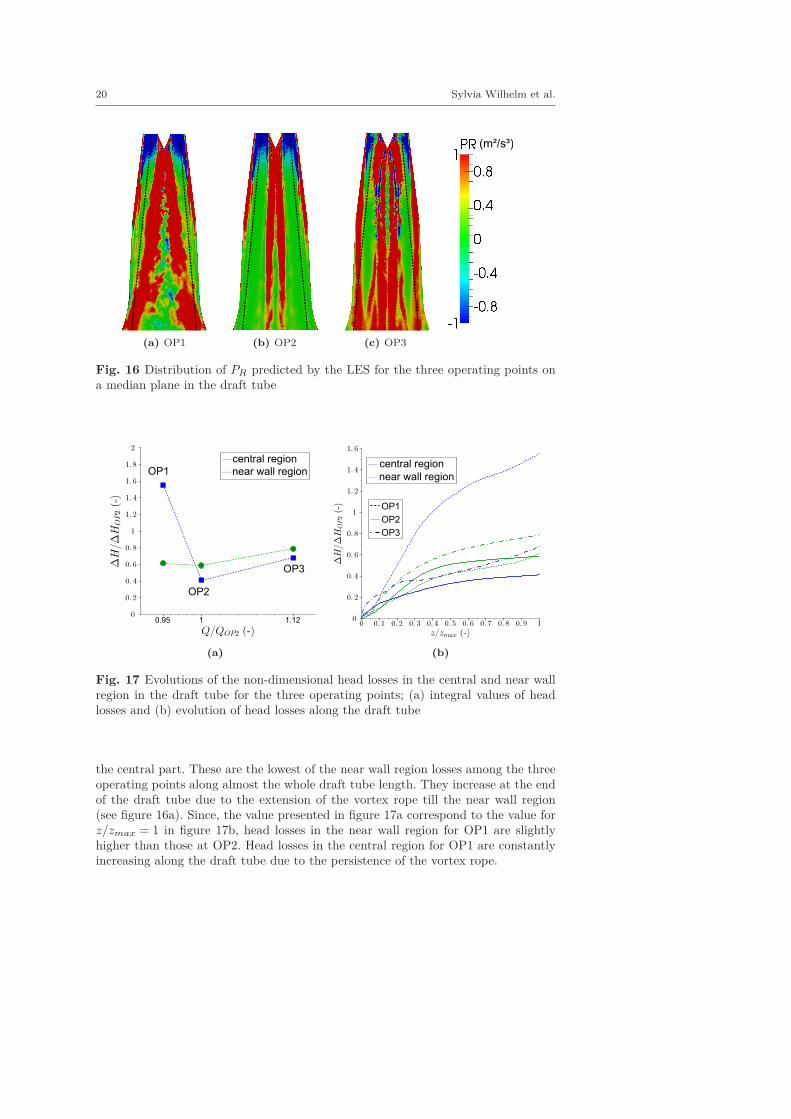
In order to better understand the different evolutions of head losses with theflow rate, the distributions of the dominating term in equation (6), PR, are shownin figure 16 on a median plane in the draft tube for OP1, OP2 and OP3. Accordingto the distributions of PR for all operating points, head losses are occurring in thecenter of the draft tube due to the central vortex structures observed in figure 9 andin the near wall region. In particular for OP1, the diverging vortex rope observed infigure 9a seems to be responsible for a large part for the losses. Turbulent productionPR is principally concentrated in the cone of the draft tube for OP2 whereas it occursalong the whole draft tube for OP1 and OP3. This is in agreement with the headlosses evolution in figure 15b.

Notice that the averaged isocurves remain quite irregular especially for the OP1and OP3 operating points. This is due to the highly intermittent turbulent flow forthese two cases. The achievement of smoother curves would require a much longertime integration but the main conclusions drawn from figure 16 would be identical.

For further analysis, the head losses evolutions are decomposed in figure 17 intohead losses in the central region and in the vicinity of the wall, as explained insection 4.2. These regions are indicated in figure 16 for clarity. Similarly to figure15b, figure 17b represents the cumulative head losses between the inlet z = 0 and agiven z location. The points shown on figure 17a therefore correspond to the valuesobtained for z/zmax = 1 in figure 17b.

From figure 17a, it is clear that the increase of head losses from OP2 to OP1is due to the central vortex structure which leads to higher turbulent productionthan at OP2. By contrast, from OP2 to OP3 head losses increase in both the centralregion and the near wall region. Similar evolutions of head losses in the central andnear wall regions are found for OP2 and OP3: head losses strongly increase in thefirst part of the draft tube and then level off. Moreover, head losses are higher inthe near wall region than in the center of the draft tube for these two points. Thisis the contrary for OP1 where head losses in the near wall region are lower than in


(a) OP1 (b) OP2 (c) OP3

(m²/s³)

Fig. 16 Distribution of PR predicted by the LES for the three operating points ona median plane in the draft tube

0.95 1 1.12

central region

near wall regionOP1

OP2

OP3

(a)

OP1

OP2

OP3

central region

near wall region

(b)

Fig. 17 Evolutions of the non-dimensional head losses in the central and near wallregion in the draft tube for the three operating points; (a) integral values of headlosses and (b) evolution of head losses along the draft tube

the central part. These are the lowest of the near wall region losses among the threeoperating points along almost the whole draft tube length. They increase at the endof the draft tube due to the extension of the vortex rope till the near wall region(see figure 16a). Since, the value presented in figure 17a correspond to the value forz/zmax = 1 in figure 17b, head losses in the near wall region for OP1 are slightlyhigher than those at OP2. Head losses in the central region for OP1 are constantlyincreasing along the draft tube due to the persistence of the vortex rope.


5 Conclusion

Unsteady RANS (URANS) simulations and Large Eddy Simulations (LES) wereperformed in the draft tube of a bulb turbine at three different operating points.Inlet boundary conditions of the draft tube accounting for the unsteadiness from therunner have been prescribed. The main objectives of the present study were (i) toevaluate the reliability of the numerical approaches and (ii) to better understand theorigin of the head losses in the draft tube.

Predicted velocity profiles in the draft tube are compared with experimentalmeasurements in order to assess the validity of the numerical simulations. Accuratetangential velocity profile at the draft tube inlet is found to be crucial for a correctflow prediction in the draft tube. For the best efficiency point of the turbine, a slightincrease of the inlet tangential velocity level exported from the guide vane - runnercalculation is thus necessary to obtain more realistic flow prediction in the draft tube.In order to properly quantify the flow sensitivity to inlet conditions, uncertaintiesquantification on the flow prediction in the draft tube will be investigated in furtherwork. For the off-design points, the velocity profiles prediction is better in the conedue to a correct inlet tangential velocity level predicted by the guide vane - runnercalculation. Flow prediction has however to be improved in the diffuser of the drafttube for the three operating points. A detailed investigation of the energy dissipationin this flow region shows that a large proportion of energy loss takes place in thevicinity of the diffuser wall. We therefore plan to perform further LES studies withmesh refinement next to the diffuser wall. URANS and LES simulations globallypredict similar large scale flow structures in the draft tube. However, LES are ableto reproduce the complexity of the vortex structures and render possible a betterunderstanding of the vortex dynamics.

Using the mean kinetic energy balance in the draft tube, the physical and hy-drodynamic phenomena responsible for head losses are identified. As expected, headlosses are mainly due to turbulent kinetic energy dissipation and thus are stronglycorrelated with the turbulent kinetic energy production from the mean kinetic energy.Head losses prediction in URANS simulations is highly dependent on the turbulencemodelling. On the other hand, the head losses are mainly controlled by the resolvedstructures in LES and only a small part of the head losses is dependent on the sub-grid scale modelled flow. The modelled part of the head losses in LES acts mainly inthe vortex rope and can be reduced by refining the mesh. This suggests that an im-provement of the head losses prediction can be expected from LES on refined mesh.This constitutes an advantage of LES, because improvement of URANS predictioncannot be expected without a complex specific tuning of the model.

Thanks to a more local analysis of the energy balance in the draft tube, thecentral vortex structure is found to be responsible for head losses, as well as veloc-ity gradients in the vicinity of the external wall. It is shown that the head lossesmechanisms are very different just downstream of the turbine, in the cone or furtherdownstream in the draft tube. This constitutes a real challenge for turbulence mod-elling since the model must be able to properly reproduce these various dissipativemechanisms in order to be predictive for the global draft tube losses. The local energybalance analysis conducted for off-design points highlights the hydrodynamic phe-nomena at the origin of poor performances of the draft tube under these operatingconditions. Under part load conditions, the helical vortex rope is thus responsible forhigh turbulent production and thus dissipation of mean kinetic energy. Conversely,


at the best efficiency and high load points, turbulent production in the near wallregion is higher than in the vortex rope. The differences in head losses between thebest efficiency point and the off-design points are principally due to higher turbulentproduction in the vortex rope under off-design conditions. The physical analysis ofhead losses presented in this study enables us to localize the regions of high headlosses. This constitutes a valuable information to optimize the draft tube design.

Acknowledgements The authors would like to thank GE Renewable Energy for the financialsupport and contribution to this project. Vincent Moureau and Ghislain Lartigue from theCORIA lab, and the SUCCESS scientific group are acknowledged for providing the YALES2code. Computations presented in this paper were performed using HPC resources from GENCI-IDRIS (Grant No. 2012-020611) and CIMENT infrastructure (supported by CPER07 13 CIRAand ANR-10-EQPX-29-01).

A Mesh influence study for URANS and LES

A.1 Mesh convergence study for URANS simulations

We have performed a classical convergence test consisting in a progressive mesh refinement.Four different meshes have been considered. First, three meshes with an identical averaged y+

value equal to 5 : mesh A with 2 million elements; mesh B with 4 million; mesh C with 10million. Second, a fourth mesh (mesh D) with 2 million of elements but a y+ value smaller than2 on each wall (mesh D) as recommended by ANSYS CFX to resolve the turbulent boundarylayer with the k − ω model.

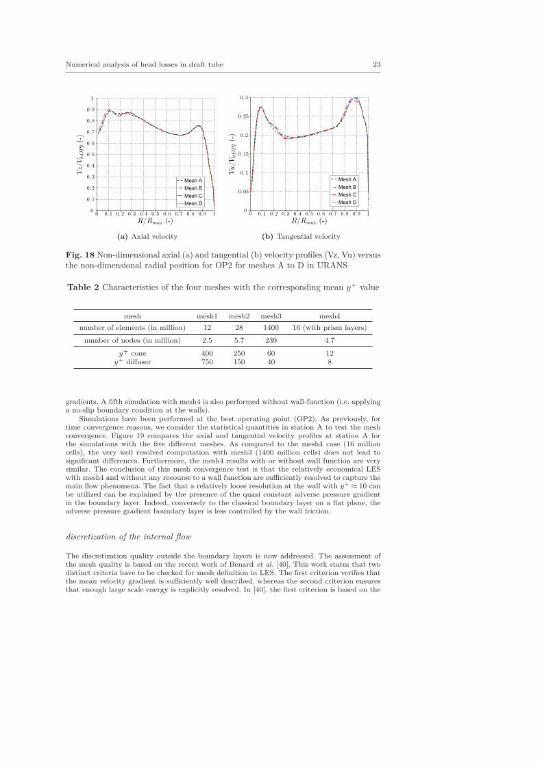
In order to more rapidly obtain converged statistics, we use station A to check the meshconvergence. A comparison of the axial and tangential velocity profiles at station A for OP2 arepresented in figure 18. The various meshes yield very close profiles. We have checked that sim-ilar results are obtained for the other operating points. The study presented in the manuscriptis thus based on URANS simulations performed using the first mesh (mesh A) since it consti-tutes an ”economical” mesh combining sufficient wall resolution and a better resolution of theinternal flow as compared with mesh D.

A.2 Mesh influence study for Large Eddy Simulations

The definition of a correct mesh for LES in complex geometries remains a challenging question.Two major points have indeed to be considered : the near-wall resolution and the discretizationof the internal flow.

Near-wall resolution

First, the near-wall resolution influence has been studied using four meshes with varying y+

but with similar mesh size in the internal flow region. The characteristics of the four differ-ent meshes are presented in table 2. The first three meshes (mesh1, mesh2 and mesh3) arecomposed of tetrahedral cells only and the mesh is refined close to the walls. Cells with a toolarge aspect ratio between the mesh size in the direction parallel to the wall and the one inthe normal direction are not allowed ought to numerical convergence criteria. Therefore, evenwith a very large number of cells of 1400 million (mesh3), the minimum y+ remains close to50. We have then used a fourth mesh (mesh4) still consisting of tetrahedral cells away fromthe wall but with layers of prismatic cells close to the walls. This procedure allows for a betterrefinement in the near wall region with y+ values close to 10. Again for numerical convergencereasons, it is not possible to go below this value with the chosen mesh. For the four simulations,we use the wall-function developed by Duprat et al. [39] for flows with strong adverse pressure


Mesh A

Mesh B

Mesh C

Mesh D

(a) Axial velocity

Mesh A

Mesh B

Mesh C

Mesh D


Fig. 18 Non-dimensional axial (a) and tangential (b) velocity profiles (Vz, Vu) versusthe non-dimensional radial position for OP2 for meshes A to D in URANS

Table 2 Characteristics of the four meshes with the corresponding mean y+ value

mesh mesh1 mesh2 mesh3 mesh4

number of elements (in million) 12 28 1400 16 (with prism layers)

number of nodes (in million) 2.5 5.7 239 4.7

y+ cone 400 250 60 12y+ diffuser 750 150 40 8

gradients. A fifth simulation with mesh4 is also performed without wall-function (i.e. applyinga no-slip boundary condition at the walls).

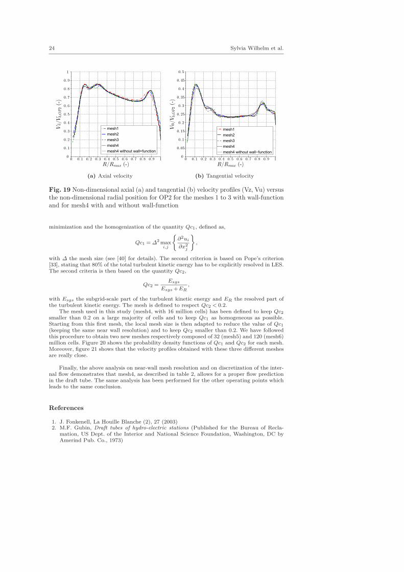
Simulations have been performed at the best operating point (OP2). As previously, fortime convergence reasons, we consider the statistical quantities in station A to test the meshconvergence. Figure 19 compares the axial and tangential velocity profiles at station A forthe simulations with the five different meshes. As compared to the mesh4 case (16 millioncells), the very well resolved computation with mesh3 (1400 million cells) does not lead tosignificant differences. Furthermore, the mesh4 results with or without wall function are verysimilar. The conclusion of this mesh convergence test is that the relatively economical LESwith mesh4 and without any recourse to a wall function are sufficiently resolved to capture themain flow phenomena. The fact that a relatively loose resolution at the wall with y+

≈ 10 canbe utilized can be explained by the presence of the quasi constant adverse pressure gradientin the boundary layer. Indeed, conversely to the classical boundary layer on a flat plane, theadverse pressure gradient boundary layer is less controlled by the wall friction.

discretization of the internal flow

The discretization quality outside the boundary layers is now addressed. The assessment ofthe mesh quality is based on the recent work of Benard et al. [40]. This work states that twodistinct criteria have to be checked for mesh definition in LES. The first criterion verifies thatthe mean velocity gradient is sufficiently well described, whereas the second criterion ensuresthat enough large scale energy is explicitly resolved. In [40], the first criterion is based on the


mesh1

mesh2

mesh3

mesh4

mesh4 without wall�function

(a) Axial velocity

mesh1

mesh2

mesh3

mesh4

mesh4 without wall−function


Fig. 19 Non-dimensional axial (a) and tangential (b) velocity profiles (Vz, Vu) versusthe non-dimensional radial position for OP2 for the meshes 1 to 3 with wall-functionand for mesh4 with and without wall-function

minimization and the homogenization of the quantity Qc1, defined as,

Qc1 = ∆2 maxi,j

{∂2ui

∂x2j

}

,

with ∆ the mesh size (see [40] for details). The second criterion is based on Pope’s criterion[33], stating that 80% of the total turbulent kinetic energy has to be explicitly resolved in LES.The second criteria is then based on the quantity Qc2,

Qc2 =Esgs

Esgs + ER

,

with Esgs the subgrid-scale part of the turbulent kinetic energy and ER the resolved part ofthe turbulent kinetic energy. The mesh is defined to respect Qc2 < 0.2.

The mesh used in this study (mesh4, with 16 million cells) has been defined to keep Qc2

smaller than 0.2 on a large majority of cells and to keep Qc1 as homogeneous as possible.Starting from this first mesh, the local mesh size is then adapted to reduce the value of Qc1

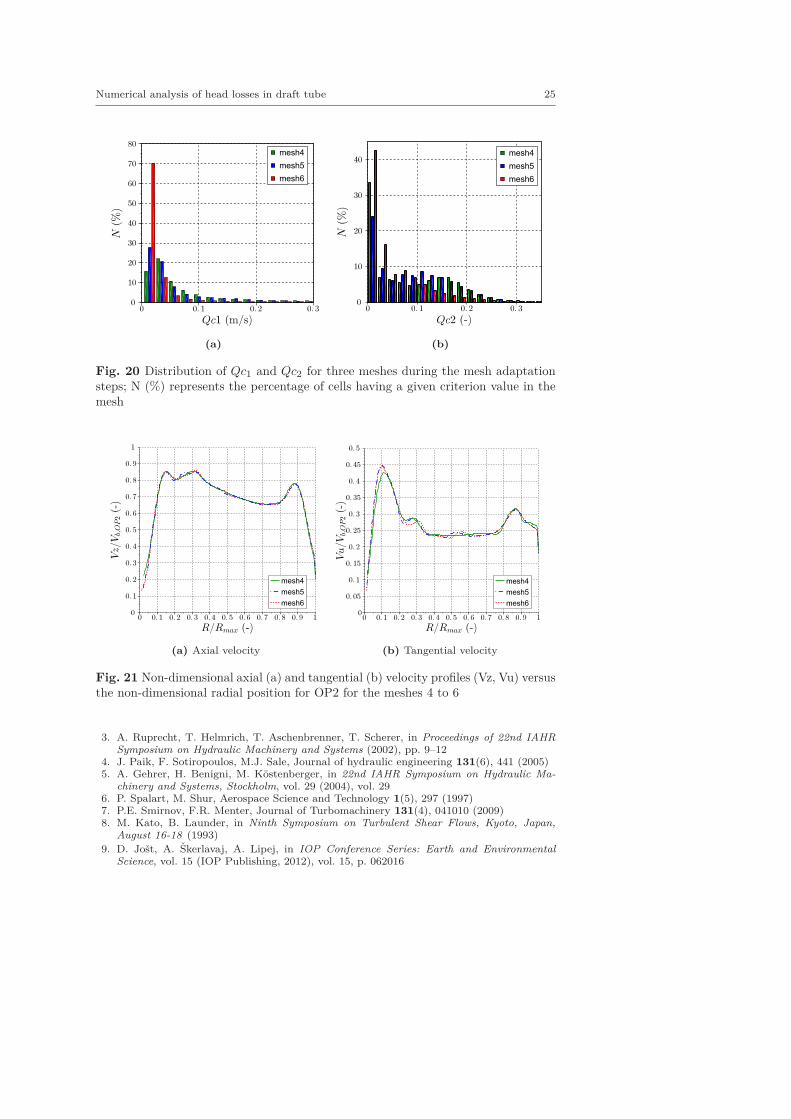
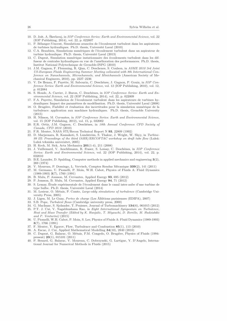
(keeping the same near wall resolution) and to keep Qc2 smaller than 0.2. We have followedthis procedure to obtain two new meshes respectively composed of 32 (mesh5) and 120 (mesh6)million cells. Figure 20 shows the probability density functions of Qc1 and Qc2 for each mesh.Moreover, figure 21 shows that the velocity profiles obtained with these three different meshesare really close.

Finally, the above analysis on near-wall mesh resolution and on discretization of the inter-nal flow demonstrates that mesh4, as described in table 2, allows for a proper flow predictionin the draft tube. The same analysis has been performed for the other operating points whichleads to the same conclusion.

References

1. J. Fonkenell, La Houille Blanche (2), 27 (2003)2. M.F. Gubin, Draft tubes of hydro-electric stations (Published for the Bureau of Recla-

mation, US Dept. of the Interior and National Science Foundation, Washington, DC byAmerind Pub. Co., 1973)


mesh4

mesh5

mesh6

(a)

mesh4

mesh5

mesh6

(b)

Fig. 20 Distribution of Qc1 and Qc2 for three meshes during the mesh adaptationsteps; N (%) represents the percentage of cells having a given criterion value in themesh

mesh4

mesh5

mesh6

(a) Axial velocity

mesh4

mesh5

mesh6


Fig. 21 Non-dimensional axial (a) and tangential (b) velocity profiles (Vz, Vu) versusthe non-dimensional radial position for OP2 for the meshes 4 to 6

3. A. Ruprecht, T. Helmrich, T. Aschenbrenner, T. Scherer, in Proceedings of 22nd IAHRSymposium on Hydraulic Machinery and Systems (2002), pp. 9–12

4. J. Paik, F. Sotiropoulos, M.J. Sale, Journal of hydraulic engineering 131(6), 441 (2005)5. A. Gehrer, H. Benigni, M. Kostenberger, in 22nd IAHR Symposium on Hydraulic Ma-

chinery and Systems, Stockholm, vol. 29 (2004), vol. 296. P. Spalart, M. Shur, Aerospace Science and Technology 1(5), 297 (1997)7. P.E. Smirnov, F.R. Menter, Journal of Turbomachinery 131(4), 041010 (2009)8. M. Kato, B. Launder, in Ninth Symposium on Turbulent Shear Flows, Kyoto, Japan,

August 16-18 (1993)9. D. Jost, A. Skerlavaj, A. Lipej, in IOP Conference Series: Earth and Environmental

Science, vol. 15 (IOP Publishing, 2012), vol. 15, p. 062016


10. D. Jost, A. Skerlavaj, in IOP Conference Series: Earth and Environmental Science, vol. 22(IOP Publishing, 2014), vol. 22, p. 022007

11. P. Belanger-Vincent, Simulations avancees de l’ecoulement turbulent dans les aspirateursde turbines hydrauliques. Ph.D. thesis, Universite Laval (2010)

12. C.A. Beaubien, Simulations numeriques de l’ecoulement turbulent dans un aspirateur deturbine hydraulique. Ph.D. thesis, Universite Laval (2013)

13. C. Duprat, Simulation numerique instationnaire des ecoulements turbulent dans les dif-fuseur de centrales hydrauliques en vue de l’amelioration des performances. Ph.D. thesis,Institut National Polytechnique de Grenoble-INPG (2010)

14. J.M. Gagnon, F. Flemming, R. Qian, C. Deschenes, S. Coulson, in ASME 2010 3rd JointUS-European Fluids Engineering Summer Meeting collocated with 8th International Con-ference on Nanochannels, Microchannels, and Minichannels (American Society of Me-chanical Engineers, 2010), pp. 2227–2236

15. V. De Henau, F. Payette, M. Sabourin, C. Deschenes, J. Gagnon, P. Gouin, in IOP Con-ference Series: Earth and Environmental Science, vol. 12 (IOP Publishing, 2010), vol. 12,p. 012084

16. S. Houde, A. Carrier, J. Buron, C. Deschenes, in IOP Conference Series: Earth and En-vironmental Science, vol. 22 (IOP Publishing, 2014), vol. 22, p. 022009

17. F.A. Payette, Simulation de l’ecoulement turbulent dans les aspirateurs de turbines hy-drauliques: Impact des parametres de modelisation. Ph.D. thesis, Universite Laval (2008)

18. O. Brugiere, Fiabilite et evaluation des incertitudes pour la simulation numerique de laturbulence: application aux machines hydrauliques. Ph.D. thesis, Grenoble University(2015)

19. H. Nilsson, M. Cervantes, in IOP Conference Series: Earth and Environmental Science,vol. 15 (IOP Publishing, 2012), vol. 15, p. 032002

20. E.R. Ortiz, J.M. Gagnon, C. Deschenes, in 18th Annual Conference CFD Society ofCanada, CFD 2010 (2010)

21. F.R. Menter, NASA STI/Recon Technical Report N 93, 22809 (1992)22. D. Marjavaara, R. Kamakoti, S. Lundstrom, S. Thakur, J. Wright, W. Shyy, in Turbine-

99 III: Proceedings of the third IAHR/ERCOFTAC workshop on draft tube flow (Lulea:Lulea tekniska universitet, 2005)

23. H. Keck, M. Sick, Acta Mechanica 201(1-4), 211 (2008)24. J. Vuillemard, V. Aeschlimann, R. Fraser, S. Lemay, C. Deschenes, in IOP Conference

Series: Earth and Environmental Science, vol. 22 (IOP Publishing, 2014), vol. 22, p.032010

25. B.E. Launder, D. Spalding, Computer methods in applied mechanics and engineering 3(2),269 (1974)

26. V. Moureau, P. Domingo, L. Vervisch, Comptes Rendus Mecanique 339(2), 141 (2011)27. M. Germano, U. Piomelli, P. Moin, W.H. Cabot, Physics of Fluids A: Fluid Dynamics

(1989-1993) 3(7), 1760 (1991)28. B. Mulu, P. Jonsson, M. Cervantes, Applied Energy 93, 695 (2012)29. P. Jonsson, B. Mulu, M. Cervantes, Applied Energy 94, 71 (2012)30. S. Lemay, Etude experimentale de l’ecoulement dans le canal inter-aube d’une turbine de

type bulbe. Ph.D. thesis, Universite Laval (2014)31. M. Lesieur, O. Metais, P. Comte, Large-eddy simulations of turbulence (Cambridge Uni-

versity Press, 2005)32. J. Ligen, M. Le Guay, Pertes de charge (Les Ãľditions parisiennes (EDIPA), 2007)33. S.B. Pope, Turbulent flows (Cambridge university press, 2000)34. G. MacIsaac, S. Sjolander, T. Praisner, Journal of Turbomachinery 134(6), 061015 (2012)35. P.T. J. Cui, V. Nagabhushana Rao, in Eight International Symposium on Turbulence,

Heat and Mass Transfer (Edited by K. Hanjalic, T. Miyauchi, D. Borello, M. Hadziabdicand P. Venturini) (2015)

36. U. Piomelli, W.H. Cabot, P. Moin, S. Lee, Physics of Fluids A: Fluid Dynamics (1989-1993)3(7), 1766 (1991)

37. F. Menter, Y. Egorov, Flow, Turbulence and Combustion 85(1), 113 (2010)38. A. Escue, J. Cui, Applied Mathematical Modelling 34(10), 2840 (2010)39. C. Duprat, G. Balarac, O. Metais, P.M. Congedo, O. Brugiere, Physics of Fluids (1994-

present) 23(1), 015101 (2011)40. P. Benard, G. Balarac, V. Moureau, C. Dobrzynski, G. Lartigue, Y. D’Angelo, Interna-

tional Journal for Numerical Methods in Fluids (2015)

Documents

Analysis of Head Losses in a Turbine Draft Tube by Means