ANALYSIS OF FOURIER TRANSFORM VALUATION FORMULAS AND ... · ANALYSIS OF FOURIER TRANSFORM VALUATION FORMULAS AND APPLICATIONS ERNST EBERLEIN, KATHRIN GLAU, AND ANTONIS PAPAPANTOLEON

arX

iv:0

809.

3405

v4 [

q-fi

n.PR

] 2

4 Se

p 20

09

ANALYSIS OF FOURIER TRANSFORM VALUATION

FORMULAS AND APPLICATIONS

ERNST EBERLEIN, KATHRIN GLAU, AND ANTONIS PAPAPANTOLEON

Abstract. The aim of this article is to provide a systematic analysis ofthe conditions such that Fourier transform valuation formulas are validin a general framework; i.e. when the option has an arbitrary payofffunction and depends on the path of the asset price process. An interplaybetween the conditions on the payoff function and the process arisesnaturally. We also extend these results to the multi-dimensional case,and discuss the calculation of Greeks by Fourier transform methods. Asan application, we price options on the minimum of two assets in Levyand stochastic volatility models.

1. Introduction

Since the seminal work of Carr and Madan (1999) and Raible (2000) onthe valuation of options with Fourier transform methods, there have beenseveral articles dealing with extensions and analysis of these valuation for-mulas. This literature focuses on the extension of the method to other situ-ations, e.g. the pricing of exotic or multi-asset derivatives, or on the analysisof the discretization error of the fast Fourier transform.

The article of Borovkov and Novikov (2002) deals with the application ofFourier transform valuation formulas for the pricing of some exotic options,while Hubalek et al. (2006) use similar techniques for hedging purposes. Lee(2004) provides an analysis of the discretization error in the fast Fouriertransform, while Lord (2008) extends the method to the pricing of optionswith early exercise features. Recently, Hubalek and Kallsen (2005), Biaginiet al. (2008) and Hurd and Zhou (2009) extend the method to accommo-date options on several assets, considering basket options, spread optionsand catastrophe insurance derivatives. Dufresne et al. (2009) also considerthe valuation of payoffs arising in insurance mathematics by Fourier meth-ods. In addition, the books of Cont and Tankov (2003), Boyarchenko and

2000 Mathematics Subject Classification. 91B28; 42B10; 60G48.Key words and phrases. option valuation; Fourier transform; semimartingales; Levy

processes; stochastic volatility models; options on several assets.We would like to thank Friedrich Hubalek and Gabriel Maresch for valuable discussions.

K. G. would like to thank the DFG for financial support through project EB66/11-1, andthe Austrian Science Fund (FWF) for an invitation under grant P18022. A. P. gratefullyacknowledges the financial support from the Austrian Science Fund (FWF grant Y328,START Prize).

We would like to thank the two anonymous referees for their careful reading of themanuscript and their valuable suggestions that have improved the paper.

1

http://arxiv.org/abs/0809.3405v4

2 E. EBERLEIN, K. GLAU, AND A. PAPAPANTOLEON

Levendorskiı (2002) and Schoutens (2003) are also discussing Fourier trans-form methods for option pricing. Let us point out that all these results areintimately related to Parseval’s formula, cf. Katznelson (2004, VI.2.2).

The aim of our article is to provide a systematic analysis of the condi-tions required for the existence of Fourier transform valuation formulas ina general framework: i.e. when the underlying variable can depend on thepath of the price process and the payoff function can be discontinuous. Suchan analysis seems to be missing in the literature.

In their work, Carr and Madan (1999), Raible (2000) and most others areusually imposing a continuity assumption, either on the payoff function oron the random variable (i.e. existence of a Lebesgue density). However, whenconsidering e.g. a one-touch option on a Levy-driven asset, both assumptionsfail: the payoff function is clearly discontinuous, while a priori not much isknown about the existence of a density for the distribution of the supremumof a Levy process. Analogous situations can also arise in higher dimensions.

The key idea in Fourier transform methods for option pricing lies in theseparation of the underlying process and the payoff function. We derive con-ditions on the moment generating function of the underlying random vari-able and the Fourier transform of the payoff function such that Fourier basedvaluation formulas hold true in one and several dimensions. An interestinginterplay between the continuity conditions imposed on the payoff functionand the random variable arises naturally. We also derive a result that allowsto easily verify the conditions on the payoff function (cf. Lemma 2.5).

The results of our analysis can be briefly summarized as follows: for gen-eral continuous payoff functions or for variables, whose distribution has aLebesgue density, the valuation formulas using Fourier transforms are validas Lebesgue integrals, in one and several dimensions. When the payoff func-tion is discontinuous and the random variable might not possess a Lebesguedensity then, in dimension one, we get pointwise convergence of the val-uation formulas under additional assumptions, that are typically satisfied.In several dimensions pointwise convergence fails, but we can deduce thevaluation function as an L2-limit.

In addition, the structure of the valuation formulas allows us to deriveeasily formulas for the sensitivities of the option price with respect to thevarious parameters; otherwise, Malliavin calculus techniques or cubature for-mulas have to be employed, cf. e.g. Fournie et al. (1999), Teichmann (2006)and Kohatsu-Higa and Yasuda (2009). We discuss results regarding the sen-sitivities with respect to the initial value, i.e. the delta and the gamma. Itturns out that the trade-off between continuity conditions on the payofffunction and the random variable established for the valuation formulas,becomes now a trade-off between integrability and smoothness conditionsfor the calculation of the sensitivities.

The valuation formulas allow to compute prices of European options veryfast, hence they allow the efficient calibration of the model to market datafor a large variety of driving processes, such as Levy processes and affinestochastic volatility models. Indeed, for Levy and affine processes the mo-ment generating function is usually known explicitly, hence these models aretailor-made for Fourier transform pricing formulas.

ANALYSIS OF VALUATION FORMULAS 3

We also mention here that the Fourier transform based approach can beapplied for the efficient computation of prices in other frameworks as well.An important area is the valuation of interest rate derivatives in Levy drivenmodels. Levy term structure models were developed in a series of papers inthe last ten years; this development is surveyed in Eberlein and Kluge (2007).For the Fourier based formulas we mention the two papers by Eberlein andKluge (2006a, 2006b), where caps, floors, and swaptions as well as interestrate digital and range digital options are discussed; furthermore Eberlein andKoval (2006), where cross currency derivatives are considered and Eberlein,Kluge, and Schonbucher (2006), where pricing formulas for credit defaultswaptions are derived. Moreover, in the framework of the ‘affine LIBOR’model (cf. Keller-Ressel et al. 2009) caps and swaptions can be easily pricedby Fourier based methods.

This paper is organized as follows: in Section 2 we present valuation for-mulas in the single asset case, and in Section 3 we deal with the valuationof options on several assets. In Section 4 we discuss sensitivities. In Section5 we review examples of commonly used payoff functions, in dimension oneand in multiple dimensions. In Section 6 we review Levy and affine pro-cesses. Finally, in Section 7 we provide numerical examples for the valuationof options on several assets in Levy and affine stochastic volatility models.

2. Option valuation: single asset

1. Let B = (Ω,F ,F, P ) be a stochastic basis in the sense of Jacod andShiryaev (2003, I.1.3), where F = FT and F = (Ft)0≤t≤T . We model theprice process of a financial asset, e.g. a stock or an FX rate, as an exponentialsemimartingale S = (St)0≤t≤T , i.e. a stochastic process with representation

St = S0eHt , 0 ≤ t ≤ T (2.1)

(shortly: S = S0eH), whereH = (Ht)0≤t≤T is a semimartingale withH0 = 0.

Every semimartingale H = (Ht)0≤t≤T admits a canonical representation

H = B +Hc + h(x) ∗ (µ− ν) + (x− h(x)) ∗ µ, (2.2)

where h = h(x) is a truncation function, B = (Bt)0≤t≤T is a predictableprocess of bounded variation, Hc = (Hc

t )0≤t≤T is the continuous martingalepart of H with predictable quadratic characteristic 〈Hc〉 = C, and ν isthe predictable compensator of the random measure of jumps µ of H. HereW ∗ µ denotes the integral process of W with respect to µ, and W ∗ (µ −ν) denotes the stochastic integral of W with respect to the compensatedrandom measure µ− ν; cf. Jacod and Shiryaev (2003, Chapter II).

Let M(P ), resp. Mloc(P ), denote the class of all martingales, resp. localmartingales, on the given stochastic basis B.

Subject to the assumption that the process 1x>1ex ∗ ν has bounded

variation, we can deduce the martingale condition

S = S0eH ∈ Mloc(P ) ⇔ B +

C

2+ (ex − 1− h(x)) ∗ ν = 0; (2.3)

cf. Eberlein et al. (2008) for details. The martingale condition can also beexpressed in terms of the cumulant process K associated to (B,C, ν), i.e.K(1) = 0; for the cumulant process see Jacod and Shiryaev (2003).


Throughout this work, we assume that P is an (equivalent) martingalemeasure for the asset S and the martingale condition is in force; moreover,for simplicity we assume that the interest rate and dividend yield are zero. Byno-arbitrage theory the price of an option on S is calculated as its discountedexpected payoff.

2. Let Y = (Yt)0≤t≤T be a stochastic process on the given basis. We denote

by Y = (Y t)0≤t≤T and Y = (Y t)0≤t≤T the supremum and the infimumprocesses of Y respectively, i.e.

Y t = sup0≤u≤t

Yu and Y t = inf0≤u≤t

Yu.

Notice that since the exponential function is monotonically increasing,the supremum processes of S and H are related via

ST = sup0≤t≤T

(S0e

Ht)= S0e

sup0≤t≤T Ht = S0eHT . (2.4)

Similarly, the infimum processes of S and H are related via

ST = S0eHT .

3. The aim of this work is to tackle the problem of efficient valuation forplain vanilla options, such as European call and put options, as well as forexotic path-dependent options, such as lookback and one-touch options, in aunified framework. Therefore, we will analyze and prove valuation formulasfor options on an asset S = S0e

H with a payoff at maturity T that maydepend on the whole path of S up to time T . These results, together withanalyticity conditions on the Wiener–Hopf factors, will be used in the com-panion paper (Eberlein, Glau, and Papapantoleon 2009) for the pricing ofone-touch and lookback options in Levy models.

The following example of a fixed strike lookback option will serve as aguideline for our methodology; note that using (2.4) it can be re-written as

(ST −K

)+=(S0e

HT −K)+. (2.5)

In order to incorporate both plain vanilla options and exotic options ina single framework we separate the payoff function from the underlyingprocess, where:

(a) the underlying process can be the log-asset price process or the supre-mum/infimum of the log-asset price process or an average of the log-assetprice process. This process will always be denoted by X (i.e. X = H orX = H or X = H, etc.);

(b) the payoff function is an arbitrary function f : R → R+, for examplef(x) = (ex −K)+ or f(x) = 1ex>B, for K,B ∈ R+.

Clearly, we regard options as dependent on the underlying process X, i.e.on (some functional of) the logarithm of the asset price process S. The mainadvantage is that the characteristic function of X is easier to handle thanthat of (some functional of) S; for example, for a Levy process H = X it isalready known in advance.

Moreover, we consider exactly those options where we can incorporate thepath-dependence of the option payoff into the underlying process X. Euro-pean vanilla options are a trivial example, as there is no path-dependence; a


non-trivial, example are options on the supremum, see again (2.4) and (2.5).Other examples are the geometric Asian option and forward-start options.

In addition, we will assume that the initial value of the underlying processX is zero; this is the case in all natural examples in mathematical finance.The initial value S0 of the asset price process S plays a particular role,because it is convenient to consider the option price as a function of it, ormore specifically as a function of s = − log S0.

Hence, we express a general payoff as

Φ(S0e

Ht , 0 ≤ t ≤ T)= f(XT − s) , (2.6)

where f is a payoff function and X is the underlying process, i.e. an adaptedprocess, possibly depending on the full history of H, with

Xt := Ψ(Hs, 0 ≤ s ≤ t) for t ∈ [0, T ],

and Ψ a measurable functional. Therefore, the time-0 price of the option isprovided by the (discounted) expected payoff, i.e.

Vf (X; s) = E[Φ(St, 0 ≤ t ≤ T

)]= E

[f(XT − s)

]. (2.7)

Note that we consider ‘European style’ options, in the sense that theholder or writer do not have the right to exercise or terminate the optionbefore maturity.

Remark 2.1. In case the interest rate r and the dividend yield δ are non-zero, then the martingale condition (2.3) reads

(δ − r)t+Bt +Ct

2+ (ex − 1− h(x)) ∗ νt = 0

for all t, and the option price is given by Vf (X; s) = e−rTE[f(XT − s)

].

4. The first result focuses on options with continuous payoff functions, suchas European plain vanilla options, but also lookback options.

Let PXTdenote the law, MXT

the moment generating function and ϕXT

the (extended) characteristic function of the random variable XT ; that is

MXT(u) = E

[euXT

]= ϕXT

(−iu),for suitable u ∈ C. For any payoff function f let g denote the dampenedpayoff function, defined via

g(x) = e−Rxf(x) (2.8)

for some R ∈ R. Let g denote the (extended) Fourier transform of a functiong, and L1

bc(R) the space of bounded, continuous functions in L1(R).In order to derive a valuation formula for an option with an arbitrary

continuous payoff function f , we will impose the following conditions.

(C1): Assume that g ∈ L1bc(R).

(C2): Assume that MXT(R) exists.

(C3): Assume that g ∈ L1(R).

Theorem 2.2. If the asset price process is modeled as an exponential semi-martingale process according to (2.1)–(2.3) and conditions (C1)–(C3) are in


force, then the time-0 price function is given by

Vf (X; s) =e−Rs

2π

∫

R

e−iusϕXT(u− iR)f(iR − u)du. (2.9)

Proof. Using (2.7) and (2.8) we have

Vf (X; s) =

∫

Ω

f(XT − s)dP = e−Rs

∫

R

eRxg(x − s)PXT(dx). (2.10)

By assumption (C1), g ∈ L1(R) and the Fourier transform of g,

g(u) =

∫

R

eiuxg(x)dx,

is well defined for every u ∈ R and is also continuous and bounded. Ad-ditionally, using assumption (C3) we immediately have that g ∈ L1

bc(R).Therefore, using the Inversion Theorem (cf. Deitmar 2004, Theorem 3.4.4),g can be inverted and g can be represented, for all x ∈ R, as

g(x) =1

2π

∫

R

e−ixug(u)du. (2.11)

Now, returning to the valuation problem (2.10) we get that

Vf (X; s) = e−Rs

∫

R

eRx

(1

2π

∫

R

e−i(x−s)ug(u)du

)PXT

(dx)

=e−Rs

2π

∫

R

eius

(∫

R

ei(−u−iR)xPXT(dx)

)g(u)du

=e−Rs

2π

∫

R

eiusϕXT(−u− iR)f(u+ iR)du, (2.12)

where for the second equality we have applied Fubini’s theorem; moreover,for the last equality we have

g(u) =

∫

R

eiuxe−Rxf(x)dx = f(u+ iR).

Finally, the application of Fubini’s theorem is justified since∫

R

∫

R

eRx|e−iu(x−s)||g(u)|duPXT(dx) ≤

∫

R

eRx

(∫

R

|g(u)|du)PXT

(dx)

≤ KMXT(R) <∞,

where we have used again that g ∈ L1(R), and the finiteness of MXT(R) is

given by Assumption (C2).

Remark 2.3. We could also replace assumptions (C1) and (C3) with thefollowing conditions

(C1′): g ∈ L1(R) and (C3′): eRxPXT∈ L1(R).


Condition (C3′) yields that eRxPXTpossesses a continuous bounded Lebesgue

density, say ρ; cf. Breiman (1968, Theorem 8.39). Then, we can identify ρ,instead of g, with the inverse of its Fourier transform and the proof goesthrough with the obvious modifications. This statement is almost identicalto Theorem 3.2 in Raible (2000).

Remark 2.4 (Numerical evaluation). The option price represented as anintegral of the form (2.9) can be evaluated numerically very fast. The fol-lowing simple observation can speed up the computation of this expressioneven further: notice that for a fixed maturity T , the characteristic function– which is the computationally expensive part – should only be evaluatedonce for all different strikes or initial values. The gain in computationaltime will be significant when considering models where the characteristicfunction is not known in closed form; e.g. in affine models where one mightneed to solve a Riccati equation to obtain the characteristic function. Thisobservation has been termed ‘caching’ by some authors (cf. Kilin 2007)

5. Apart from (C3), the prerequisites of Theorem 2.2 are quite easy to checkin specific cases. In general, it is also an interesting question to know whenthe Fourier transform of an integrable function is integrable. The problem iswell understood for smooth (C2 or C∞) functions, see e.g. Deitmar (2004),but the functions we are dealing with are typically not smooth. Hence, wewill provide below an easy-to-check condition for a non-smooth function tohave an integrable Fourier transform.

Let us consider the Sobolev space H1(R), with

H1(R) =g ∈ L2(R)

∣∣∣ ∂g exists and ∂g ∈ L2(R),

where ∂g denotes the weak derivative of a function g; see e.g. Sauvigny(2006). Let g ∈ H1(R), then from Proposition 5.2.1 in Zimmer (1990) weget that

∂g(u) = −iug(u) (2.13)

and g, ∂g ∈ L2(R).

Lemma 2.5. Let g ∈ H1(R), then g ∈ L1(R).

Proof. Using the above results, we have that

∞ >

∫

R

(∣∣g(u)∣∣2 +

∣∣∂g(u)∣∣2)du =

∫

R

∣∣g(u)∣∣2(1 + |u|2

)du. (2.14)

Now, by the Holder inequality, using (1 + |u|)2 ≤ 3(1 + |u|2) and (2.14), weget that

∫

R

∣∣g(u)∣∣du =

∫

R

∣∣g(u)∣∣1 + |u|1 + |u|du

≤(∫

R

∣∣g(u)∣∣2(1 + |u|)2du

)1

2

(∫

R

1

(1 + |u|)2du) 1

2

<∞

and the result is proved.


Remark 2.6. A similar statement can be proved for functions in the Sobolev-Slobodeckij space Hs(R), for s > 1

2 .

6. Next, we deal with the valuation formula for options whose payoff func-tion can be discontinuous, while at the same time the measure PXT

does notnecessarily possess a Lebesgue density. Such a situation arises typically whenpricing one-touch options in purely discontinuous Levy models. Hence, weneed to impose different conditions, and we derive the valuation formula asa pointwise limit by generalizing the proof of Theorem 3.2 in Raible (2000).A similar result (Theorem 1 in Dufresne et al. 2009) has been pointed outto us by one of the referees.

In this and the following sections we will make use of the following nota-tion; we define the function g and the measure as follows

g(x) := g(−x) and (dx) := eRxPXT(dx).

Moreover (R) =∫(dx), while g∗ denotes the convolution of the function

g with the measure . In this case we will use the following assumptions.

(D1): Assume that g ∈ L1(R).(D2): Assume that MXT

(R) exists (⇐⇒ (R) <∞).

Theorem 2.7. Let the asset price process be modeled as an exponentialsemimartingale process according to (2.1)–(2.3) and conditions (D1)–(D2)be in force. The time-0 price function is given by

Vf (X; s) = limA→∞

e−Rs

2π

A∫

−A

e−iusϕXT(u− iR)f(iR− u)du, (2.15)

at the point s ∈ R, if Vf (X; ·) is of bounded variation in a neighborhood ofs, and Vf (X; ·) is continuous at s.

Remark 2.8. In Section 5 we will relate the conditions on the valuationfunction Vf to properties of the measure PXT

for specific (dampened) payofffunctions g. These properties are easily checkable – and typically satisfied –in many models.

Proof. Starting from (2.10), we can represent the option price function as aconvolution of g and as follows

Vf (X; s) = e−Rs

∫

R

eRxg(x− s)PXT(dx) = e−Rs

∫

R

g(s − x)(dx)

= e−Rs g ∗ (s). (2.16)

Using that g ∈ L1(R), hence also g ∈ L1(R), and (R) < ∞ we get thatg ∗ ∈ L1(R), since

‖g ∗ ‖L1(R) ≤ (R) ‖g‖L1(R) <∞; (2.17)

compare with Young’s inequality, cf. Katznelson (2004, IV.1.6). Therefore,the Fourier transform of the convolution is well defined and we can deducethat, for all u ∈ R,

g ∗ (u) = g(u) · (u);


compare with Theorem 2.1.1 in Bochner (1955).By (2.17) we can apply the inversion theorem for the Fourier transform,

cf. Satz 4.2.1 in Doetsch (1950), and get

1

2

(g ∗ (s+) + g ∗ (s−)

)=

1

2πlim

A→∞

A∫

−A

e−ius (u)g(u)du, (2.18)

if there exists a neighborhood of s where s 7→ g∗(s) is of bounded variation.We proceed as follows: first we show that the function s 7→ g ∗ (s) has

bounded variation; then we show that this map is also continuous, whichyields that the left hand side of (2.18) equals g ∗ (s).

For that purpose, we re-write (2.16) as

g ∗ (s) = eRsVf (X; s);

then, g ∗ is of bounded variation on a compact interval [a, b] if and only ifVf (X; ·) ∈ BV ([a, b]); this holds because the map s 7→ eRs is of bounded vari-ation on any bounded interval on R, and the fact that the space BV ([a, b])forms an algebra; cf. Satz 91.3 in Heuser (1993). Moreover, s is a continuitypoint of g ∗ if and only if Vf (X; ·) is continuous at s .

In addition, we have that

g(u) =∫

R

e−iuxe−Rxf(x)dx = f(iR − u) (2.19)

and

(u) =∫

R

eiuxeRxPXT(dx) = ϕXT

(u− iR). (2.20)

Hence, (2.18) together with (2.19), (2.20) and the considerations regardingthe continuity and bounded variation properties of the value function yieldthe required result.

3. Option valuation: multiple assets

1. We would like to establish valuation formulas for options that depend onseveral assets or on multiple functionals of one asset. Typical examples ofoptions on several assets are basket options and options on the minimum ormaximum of several assets, with payoff

(S1T ∧ · · · ∧ Sd

T −K)+,

where x ∧ y = minx, y. Typical examples of options on functionals of asingle asset are barrier options, with payoff

(ST −K)+1ST>B,

and slide-in or corridor options, with payoff

(ST −K)+N∑

i=1

1L<STi<H,

at maturity T , where 0 = T0 < T1 < · · · < TN = T .


In the previous section we proved that the valuation formulas for a singleunderlying is still valid – at least as a pointwise limit, under reasonableadditional assumptions – even if the underlying distribution does not possessa Lebesgue density and the payoff is discontinuous.

In the present section we will generalize the valuation formulas to the caseof several underlyings. Once again, if either the joint distribution possessesa Lebesgue density or the payoff function is continuous, the formula is validas a Lebesgue integral. In case both assumptions fail, we will encountersituations that are apparently of harmless nature, but where the pointwiseconvergence will fail. In this case we will establish the valuation formulasas an L2-limit; however, with respect to numerical evaluation, a strongernotion of convergence would be preferable.

Analogously to the single asset case we assume that the asset prices evolveas exponential semimartingales. Let the driving process be an Rd-valuedsemimartingale H = (H1, . . . ,Hd)⊤ and S = (S1, . . . , Sd)⊤ be the vectorof asset price processes; then each component S i of S is modeled as anexponential semimartingale, i.e.

S i

t = S i

0 expHi

t , 0 ≤ t ≤ T , 1 ≤ i ≤ d, (3.1)

where H i is an R-valued semimartingale with canonical representation

H i = H i

0 +B i +H i ,c + hi (x) ∗ (µ− ν) + (xi − hi (x)) ∗ µ, (3.2)

with hi (x) = e⊤ih(x). The martingale condition can be given as in eq. (3.3)

in Eberlein, Papapantoleon, and Shiryaev (2009).

2. In the sequel, we will price options with payoff f(XT − s) at maturity T ,where XT is an FT -measurable Rd-valued random variable, possibly depen-dent of the history of the d driving processes, i.e.

XT = Ψ(Ht, 0 ≤ t ≤ T

),

where Ψ is an Rd-valued measurable functional. Further f is a measurablefunction f : Rd → R+, and s = (s1, . . . , s

d) ∈ Rd with si = − logS i

0.Analogously to the single asset case, we use the dampened payoff function

g(x) := e−〈R,x〉f(x) for x ∈ Rd,

and denote by the measure defined by

(dx) := e〈R,x〉PXT(dx),

where R ∈ Rd serves as a dampening coefficient. Here 〈·, ·〉 denotes theEuclidian scalar product in Rd. The scalar product is extended to Cd asfollows: for u, v ∈ Cd, set 〈u, v〉 =∑i uivi, i.e. we do not use the Hermitianinner product. Moreover, MXT

and ϕXTdenote the moment generating,

resp. characteristic, function of the random vector XT .To establish our results we will make use of the following assumptions.

(A1): Assume that g ∈ L1(Rd).(A2): Assume that MXT

(R) exists.(A3): Assume that ∈ L1(Rd).

Remark 3.1. We can also replace Assumptions (A1) and (A3) with thefollowing assumption


(A1′): Assume that g ∈ L1bc(R

d) and g ∈ L1(Rd);

this shows again the interplay between the continuity properties of the payofffunction and the underlying distribution.

Theorem 3.2. If the asset price processes are modeled as exponential semi-martingale processes according to (3.1)–(3.2) and conditions (A1)–(A3) arein force, then the time-0 price function is given by

Vf (X; s) =e−〈R,s〉

(2π)d

∫

Rd

e−i〈u,s〉MXT(R+ iu)f(iR− u)du. (3.3)

Proof. Similarly to the one-dimensional case we have that

Vf (X; s) = e−〈R,s〉g ∗ (s). (3.4)

Since g ∈ L1(Rd) and (Rd) < ∞, we get that g ∗ ∈ L1(Rd); thereforeg ∗ (u) = g(u)· (u) for all u ∈ Rd. By assumption we know that ∈ L1(Rd);moreover g ∈ L∞(Rd) since |g| ≤ ‖g‖L1(Rd) <∞. These considerations yield

that g ∗ ∈ L1(Rd), again by using Young’s inequality.Hence, applying the formula for the Fourier inversion, cf. Corollary 1.21

in Stein and Weiss (1971), we conclude that

Vf (X; s) =e−〈R,s〉

(2π)d

∫

Rd

e−i〈u,s〉g(u)(u)du

=e−〈R,s〉

(2π)d

∫

Rd

e−i〈u,s〉MXT(R+ iu)f(iR− u)du,

for a.e. s ∈ Rd.Moreover, if s 7→ Vf (X; s) is continuous, then the equality holds pointwise

for all s ∈ Rd. The mapping (3.4) is continuous if the mapping s 7→ g ∗ (s)is continuous. Using Assumption (A3) we have that possesses a boundedcontinuous Lebesgue density ρ ∈ L1(Rd); cf. Proposition 2.5 (xii) in Sato(1999). Then g ∗ = g ∗ ρ and

lim|x|→0

g ∗ (s + x) = lim|x|→0

∫g(s + x− z)ρ(z)dz

=

∫lim|x|→0

g(s + y)ρ(x− y)dy = g ∗ (s) (3.5)

yielding the continuity of the map. Note that we have used the continuity ofρ; additionally, we can interchange integration and limit using the dominatedconvergence theorem, with majorant g(·)maxx ρ(x).

Remark 3.3. The proof using Assumption (A1′) follows analogously, withthe obvious modifications for (3.5).

3. Next, we consider the valuation of options on several assets when thepayoff function is discontinuous and the driving process does not necessarilypossess a Lebesgue density.

The main difference to the analogous situation in dimension one is thatthe pointwise convergence of capped Fourier integrals – as is the case in Satz


4.2.1 in Doetsch (1950) – cannot be generalized to the multidimensional case.M. Pinsky gives the following astonishing example to illustrate this fact, seesection 4.1 in Pinsky (1993); let f be the indicator function of the unit ballin R3, then

1

(2π)3

∫

|x|≤A

e−i〈u,x〉f(x)dx∣∣∣u=0

= 1− 2

πsin(A) + o(1), (3.6)

for A ↑ ∞. Extrapolating the convergence results from the one-dimensionalcase to R3, we would expect pointwise convergence of the spherical sum tothe indicator function, at least in the interior of the ball; on the contrary,the right hand side of (3.6) is even divergent.

As a consequence, we only derive an L2-limit for the valuation function.The setting is similar to the previous sections, and we need to impose the

following conditions.

(G1): Assume that g ∈ L1(Rd) ∩ L2(Rd).(G2): Assume that MXT

(R) exists.

Theorem 3.4. If the asset price process is modeled as an exponential semi-martingale process according to (3.1)–(3.2) and conditions (G1)–(G2) are inforce, then the time-0 price function satisfies

Vf (X; ·) = e−〈R,·〉

(2π)dL2- limA→∞

∫

[−A,A]d

e−i〈u,·〉ϕXT(u− iR)f(iR− u)du. (3.7)

Proof. Similarly to the previous section, we have that

Vf (X; s) = e−〈R,s〉g ∗ (s), (3.8)

and, for all u ∈ Rd

g ∗ (u) = g(u) · (u). (3.9)

Now, since g ∈ L1(Rd) ∩ L2(Rd), we get that g ∈ L2(Rd) and ‖g‖L2(Rd) =

‖g‖L2(Rd); the proofs are analogous to Theorem 9.13 in Rudin (1987). More-

over, we have that g ∗ ∈ L2(Rd), because

‖g ∗ ‖2L2(Rd) ≤ (Rd)2 ‖g‖2L2(Rd) <∞.

Therefore, since also g ∗ ∈ L1(Rd) we get that g ∗ ∈ L1(Rd) ∩ L2(Rd)and, analogously again to Theorem 9.13 in Rudin (1987), we get that g ∗ ∈L2(Rd) and ‖g ∗ ‖L2(Rd) = ‖ g ∗ ‖L2(Rd).

Therefore, the Fourier transform in (3.9) can be inverted and the inversionis given as an L2-limit; more precisely, we have

‖g ∗ − ψA‖L2(Rd) → 0 (A→ ∞) (3.10)

where

ψA(s) =1

(2π)d

∫

[−A,A]d

e−i〈u,s〉 g ∗ (u)du

=1

(2π)d

∫

[−A,A]d

e−i〈u,s〉f(iR− u)ϕXT(u− iR)du. (3.11)


Finally, (3.8) and (3.10)–(3.11) yield the option price function.

Remark 3.5. The problem becomes significantly simpler when dealing withthe product f1(XT )f2(YT ) of a continuous payoff function f1 for the vari-able X and a discontinuous payoff function f2 for the other variable Y , evenin the absence of Lebesgue densities. A typical example of this situation isthe barrier option payoff, where f1(x) = (ex − K)+ and f2(y) = 1ey>B.Then, one can make a measure change using the (normalized) continuouspayoff as the Radon–Nikodym derivative, apply Theorem 2.2 and then The-orem 2.7; this leads to pointwise convergence of the valuation function. Themeasure change argument is outlined in Borovkov and Novikov (2002) andPapapantoleon (2007, Theorem 3.5).

4. Sensitivities – Greeks

The structure of the asset price model as an exponential semimartingale,and the resulting structure of the option price function, allows us to easilyderive general formulas for the sensitivities of the option price with respectto model parameters. In this section we will focus on the sensitivities withrespect to the initial value, i.e. delta and gamma, while sensitivities withrespect to other parameters can be derived analogously.

Let us rewrite the option price function as a function of the initial value,using that S0 = e−s , as follows:

Vf (X;S0) =1

2π

∫

R

SR−iu0 MXT

(R − iu)f(u+ iR)du. (4.1)

The delta of an option is the partial derivative of the price with respect tothe initial value. For a generic option with payoff f , we have that

∆f (X;S0) =∂Vf (X;S0)

∂S0

=1

2π

∫

R

∂

∂S0SR−iu0 MXT

(R− iu)f(u+ iR)du

=1

2π

∫

R

SR−1−iu0 MXT

(R− iu)f(u+ iR)

(R − iu)−1du. (4.2)

The gamma of an option is the partial derivative of the delta with respectto the initial value. For a generic option with payoff f , we get

Γf (X;S0) =∂∆f (X;S0)

∂S0=∂2Vf (X;S0)

∂2S0

=1

2π

∫

R

SR−2−iu0

MXT(R− iu)f(u+ iR)

(R− 1− iu)−1(R − iu)−1du. (4.3)

In the above equations we have taken for granted that we can exchangeintegration and differentiation; however, this is the crucial step and we willprovide sufficient conditions when we are allowed to do that. Using SatzIV.5.7 in Elstrodt (1999) and the elementary inequality |Imf |+|Ref | ≤ 2|f |,


we get that we can differentiate under the integral sign if there exists anintegrable function ℘ such that for all u ∈ R and all S0 > 0

∣∣∣ ∂∂S0

F (u, S0)∣∣∣ ≤ ℘(u),

where

F (u, S0) = SR−iu0 MXT

(R− iu)f(u+ iR).

Now we can estimate the partial derivative of the function F :∣∣∣ ∂∂S0

F (u, S0)∣∣∣ = |e(R−1−iu) logS0 ||R− iu||MXT

(R− iu)f(u+ iR)|

≤ c(1 + |u|)|MXT(R− iu)||f (u+ iR)| =: ℘(u). (4.4)

Analogously we can estimate for the second derivative of F :∣∣∣ ∂

2

∂S20

F (u, S0)∣∣∣ ≤ c

′(1 + |u|2)|MXT(R − iu)||f(u+ iR)| =: ℘′(u). (4.5)

Sufficient conditions for the function ℘ in (4.4), resp. ℘′ in (4.5), to beintegrable are that |u||MXT

(R− iu)|, resp. |u|2|MXT(R− iu)|, is integrable

and f(·+ iR) is bounded; the first condition dictates in particular that themeasure PXT

– equivalently – has a density of class C1, resp. C2; seeProposition 28.1 in Sato (1999). Alternatively, a sufficient condition is that

the function |u||f(u+iR)|, resp. |u|2|f(u+iR)|, is integrable andMXT(R−i·)

is bounded, highlighting once again the interplay between the properties ofthe measure and the payoff function.

5. Examples of payoff functions

1. Here we list some representative examples of payoff functions used in fi-nance, together with their Fourier transforms and comment on whether theysatisfy some of the required assumptions for option pricing. The calculationsfor the call option are provided explicitly and for other options they followalong the same lines.

Example 5.1 (Call and put option). The payoff of the standard call optionwith strike K ∈ R+ is f(x) = (ex −K)+. Let z ∈ C with ℑz ∈ (1,∞), thenthe Fourier transform of the payoff function of the call option is

f(z) =

∫

R

eizx(ex −K)+dx =

∞∫

lnK

e(1+iz)xdx−K

∞∫

lnK

eizxdx

= −K1+iz 1

1 + iz+KizK

iz=

K1+iz

iz(1 + iz). (5.1)

Now, regarding the dampened payoff function of the call option, we easilyget for R ∈ (1,∞) that g ∈ L1

bc(R) ∩ L2(R). The weak derivative of g is

∂g(x) =

0, if x < lnK,e−Rx(ex −Rex +RK), if x > lnK.

(5.2)

Again, we have that ∂g ∈ L2(R). Therefore, g ∈ H1(R) and using Lemma2.5 we can conclude that g ∈ L1(R). Summarizing, conditions (C1) and (C3)of Theorem 2.2 are fulfilled for the payoff function of the call option.


Similarly, for a put option, where f(x) = (K − ex)+, we have that

f(z) =K1+iz

iz(1 + iz), ℑz ∈ (−∞, 0). (5.3)

Analogously to the case of the call option, we can conclude for the dampenedpayoff function of the put option that g ∈ L1

bc(R) and g ∈ H1(R) for R < 0,yielding g ∈ L1(R). Hence, conditions (C1) and (C3) of Theorem 2.2 arealso fulfilled for the payoff function of the put option.

Example 5.2 (Digital option). The payoff of a digital call option withbarrier B ∈ R+ is 1ex>B. Let z ∈ C with ℑz ∈ (0,∞), then the Fouriertransform of the payoff function of the digital call option is

f(z) = −Biz

iz. (5.4)

Similarly, for a digital put option, where f(x) = 1ex<B, we have that

f(z) =Biz

iz, ℑz ∈ (−∞, 0). (5.5)

For the dampened payoff function of the digital call and put option, we caneasily check that g ∈ L1(R) for R ∈ (0,∞) and R ∈ (−∞, 0).

Regarding the continuity and bounded variation properties of the valuefunction, we have that

Vf (X, s) = E[1eXT −s>B

]= P

(XT > log(B) + s

)= 1− FXT

(log(B) + s

),

where FXTdenotes the cumulative distribution function of XT . Therefore,

s 7→ Vf (X, s) is monotonically decreasing, hence it has locally boundedvariation. Moreover, we can conclude that s 7→ Vf (X, s) is continuous if themeasure PXT

is atomless.Summarizing, condition (D1) is always satisfied for the payoff function of

the digital option, while the prerequisites of Theorem 2.7 on continuity andbounded variation are satisfied if the measure PXT

does not have atoms.

Example 5.3. A variant of the digital option is the so-called asset-or-nothing digital, where the option holder receives one unit of the asset, insteadof currency, depending on whether the underlying reaches some barrier ornot. The payoff of the asset-or-nothing digital call option with barrier B ∈R+ is f(x) = ex1ex>B, and the Fourier transform, for z ∈ C with ℑz ∈(1,∞), is

f(z) = −B1+iz

1 + iz. (5.6)

Arguing analogously to the previous example, we can deduce that condition(D1) is always satisfied for the payoff function of the asset-or-nothing digitaloption, while the prerequisites of Theorem 2.7 are satisfied if the measurePXT


Example 5.4 (Double digital option). The payoff of the double digital calloption with barriers B,B > 0 is 1B<ex<B. Let z ∈ C\0, then the Fourier

transform of the payoff function is

f(z) =1

iz

(B

iz −Biz). (5.7)


The dampened payoff function of the double digital option satisfies g ∈L1(R) for all R ∈ R.

Moreover, we can decompose the value function of the double digital op-tion as

Vf (X, s) = Vf1(X, s)− Vf2(X, s),

where f1(x) = 1ex<B and f2(x) = 1B≤ex. Hence, by the results of Exam-

ple 5.2, we get that condition (D1) is always satisfied for the payoff functionof the double digital option, while the prerequisites of Theorem 2.7 are sat-isfied if the measure PXT


Example 5.5 (Self-quanto and power options). The payoff of a self-quantocall option with strike K ∈ R+ is f(x) = ex(ex−K)+. The Fourier transformof the payoff function of the self-quanto call option, for z ∈ C with ℑz ∈(2,∞), is

f(z) =K2+iz

(1 + iz)(2 + iz). (5.8)

The payoff of a power call option with strike K ∈ R+ and power 2 is f(x) =[(ex −K)+]2; for z ∈ C with ℑz ∈ (2,∞), the Fourier transform is

f(z) = − 2K2+iz

iz(1 + iz)(2 + iz). (5.9)

The payoff functions for the respective put options are defined in the obvi-ous way, while the Fourier transforms are identical, with the range for theimaginary part of z being respectively (−∞, 1) and (−∞, 0).

Analogously to Example 5.1, we can deduce that conditions (C1) and(C3) of Theorem 2.2 are fulfilled for the payoff function of the self-quantoand the power option.

Remark 5.6. For power options of higher order we refer to Raible (2000,Chapter 3).

2. Next we present some examples of payoff functions for options on severalassets and for options on multiple functionals of one asset, together withtheir corresponding Fourier transforms.

Example 5.7 (Option on the minimum/maximum). The payoff function ofa call option on the minimum of d assets is

f(x) = (ex1 ∧ · · · ∧ exd −K)+,

for x ∈ Rd. The Fourier transform of this payoff function is

f(z) = − K1+iPd

k=1zk

(−1)d(1 + i∑d

k=1 zk)∏d

k=1(izk), (5.10)

where z ∈ Cd with ℑzk > 0 for 1 ≤ k ≤ d and ℑ(∑dk=1 zk) > 1; for more

details we refer to Appendix A. Then, we can easily deduce for the dampenedpayoff function that g ∈ L1

bc(Rd).

Moreover, for the put option on the maximum of d assets, the payofffunction is

f(x) = (K − ex1 ∨ · · · ∨ exd)+,


for x ∈ Rd, where a ∨ b = maxa, b. The Fourier transform is

f(z) =K1+i

Pdk=1

zk

(1 + i∑d

k=1 zk)∏d

k=1(izk), (5.11)

with the restriction now being ℑzk < 0 for all 1 ≤ k ≤ d. Again, we can easilydeduce that the dampened payoff function satisfies g ∈ L1

bc(Rd). Therefore,

condition (A1) of Theorem 3.2 is satisfied.

Example 5.8. A natural example of multi-asset payoff functions are prod-ucts of single asset payoff functions. These payoff functions have the form

f(x) =

d∏

i=1

fi(xi ),

for x ∈ Rd, where xi ∈ R and fi : R → R+, for all 1 ≤ i ≤ d; for example,one can consider f1(x1) = (ex1 −K)+ and f2(x2) = 1ex2>B.

The Fourier transform of these payoff functions is simply the product ofthe Fourier transform of the ‘marginal’ payoff functions, since

f(z) =

∫

Rd

ei〈z,x〉d∏

i=1

fi(xi )dx =d∏

i=1

∫

R

eizixifi(xi )dxi =d∏

i=1

fi(zi ),

for z ∈ Cd and zi ∈ C, with ℑz in an appropriate range such that g ∈ L1(Rd).

This range, as well as other properties of f , are dictated by the corresponding

properties of the Fourier transforms fi of the marginal payoff functions fi .

Remark 5.9. Further examples of multiple asset payoff functions, such asbasket and spread options, and their Fourier transforms can be found inHubalek and Kallsen (2005).

3. We add a short remark on the rate of decay of the Fourier transform of thevarious payoff functions and its consequence for numerical implementations.

Consider the standard call option, where the Fourier transform of thedampened payoff function has the form, cf. (5.1),

g(u) =K1−Reiu logK

(R − iu)(R − 1− iu), u ∈ R.

Then, we have that

|g(u)| ≤ K1−R

√R2 + u2

√(R− 1)2 + u2

≤ K1−R

(R− 1)2 + u2,

which shows that g(u) behaves like 1u2 for |u| > 1. On the other hand, a

similar calculation for the digital option shows that the Fourier transformof the dampened digital payoff behaves like 1

u for |u| > 1.Therefore, splitting a call option into the difference of an asset-or-nothing

digital and a digital option, as many authors have proposed in the literature(cf. e.g. Heston 1993), is not only ‘conceptually’ sub-optimal, as can be seenby Theorems 2.2 and 2.7. More importantly, it is also not optimal from thenumerical perspective, since the rate of decay for the digital option is muchslower than for the call option, leading to slower numerical evaluation of thecorresponding option prices.


Indeed, we have calculated the prices of call options corresponding to 11strikes and 10 maturities, first using the formula for the call option, andthen representing the call option as the difference of two digital options.The numerical calculation using the second method lasts twice as long (6secs compared to less than 3 secs) in a standard Matlab implementation.

6. Examples of driving processes

The application of Fourier transform valuation formulas in practice re-quires the explicit knowledge of the moment generating function of theunderlying random variable. As such, Fourier methods are tailor-made forpricing European options in Levy and affine models, since in these modelsone typically knows the moment generating function explicitly (at least upto the solution of a Riccati equation). In order to give a flavor, we presenthere an overview of Levy and affine processes, referring to the literature forspecific formulas and proofs.

In Levy processes, the moment generating function of the random variableis described by the celebrated Levy–Khintchine formula; for a Levy processH = (Ht)0≤t≤T with triplet (b, c, λ) we have:

E[e〈u,Ht〉

]= exp (κ(u) · t) , (6.1)

for suitable u ∈ Rd, where the cumulant generating function is

κ(u) = 〈b, u〉+ 1

2〈u, cu〉 +

∫

Rd

(e〈u,x〉 − 1− 〈u, h(x)〉

)λ(dx); (6.2)

here h denotes a suitable truncation function. The most popular Levy mod-els are the VG and CGMY processes (cf. Madan and Seneta 1990, Carr etal. 2002), the hyperbolic, NIG and GH processes (cf. Eberlein and Keller1995, Barndorff-Nielsen 1998, Eberlein 2001), and the Meixner model (cf.Schoutens and Teugels 1998).

In affine processes, the moment generating functions are described by thevery definition of these processes. Let X = (Xt)0≤t≤T be an affine process onthe state space D = Rm×Rn

+ ⊆ Rd, starting from x ∈ D; i.e., under suitable

conditions, there exist functions φ : [0, T ] × I → R and ψ : [0, T ] × I → Rd

such that

Ex

[e〈u,Xt〉

]= exp (φt(u) + 〈ψt(u), x〉) , (6.3)

for all (t, u, x) ∈ [0, T ] × I × D, I ⊆ Rd. The functions φ and ψ satisfygeneralized Riccati equations, while their time derivatives

F (u) =∂

∂t

∣∣t=0

φt(u) and R(u) =∂

∂t

∣∣t=0

ψt(u),

are of Levy–Khintchine form (6.2); we refer to Duffie et al. (2003) and Keller-Ressel (2008) for comprehensive expositions and the necessary details. Theclass of affine processes contains as special cases – among others – many sto-chastic volatility models, such as the Heston (1993) model, the BNS model(cf. Barndorff-Nielsen and Shephard 2001, Nicolato and Venardos 2003), andtime-changed Levy models (cf. Carr et al. 2003, Kallsen 2006).


7. Numerical illustration

As an illustration of the applicability of Fourier-based valuation formulaseven for the valuation of options on several assets, we present a numericalexample on the pricing of an option on the minimum of two assets. As drivingmotions we consider a 2d normal inverse Gaussian (NIG) Levy process anda 2d affine stochastic volatility model.

Let H denote a 2d NIG random variable, i.e.

H = (H1,H2) ∼ NIG2(α, β, δ, µ,∆),

where the parameters have the following domain of definition: α, δ ∈ R+,β, µ ∈ R2, and ∆ ∈ R2×2 is a symmetric, positive-definite matrix; w.l.o.g. wecan assume that det(∆) = 1; in addition, α2 > 〈β,∆β〉. Then, the momentgenerating function of H, for u ∈ R2 with α2 − 〈β + u,∆(β + u)〉 ≥ 0, is

MH(u) = exp(〈u, µ〉+ δ

(√α2 − 〈β,∆β〉 −

√α2 − 〈β + u,∆(β + u)〉

)).

(7.1)

In the NIG2 model, we specify the parameters α, β, δ and ∆, and the driftvector µ is determined by the martingale condition. Note that the marginalsH i are also NIG distributed (cf. Blæsild 1981, Theorem 1), hence the driftvector can be easily evaluated from the cumulant of the univariate NIGlaw. The covariance matrix corresponding to the NIG2-distributed randomvariable H is

ΣNIG = δ(α2 − 〈β,∆β〉

)− 1

2

(∆+

(α2 − 〈β,∆β〉

)−1∆ββ⊤∆

),

cf. Prause (1999, eq. (4.15)). A comprehensive exposition of the multivariategeneralized hyperbolic distributions can be found in Blæsild (1981); cf. alsoPrause (1999).

We will also consider the following affine stochastic volatility model intro-duced by Dempster and Hong (2002), that extends the framework of Heston(1993) to the multi-asset case. Let H = (H1,H2) denote the logarithm ofthe asset price processes S = (S1, S2), i.e. H i = log S i ; then, H i , i = 1, 2satisfy the following SDEs:

dH1t = −1

2σ21vtdt+ σ1

√vtdW

1t

dH2t = −1

2σ22vtdt+ σ2

√vtdW

2t

dvt = κ(µ− vt)dt+ σ3√vtdW

3t ,

with initial valuesH10 ,H

20 , v0 > 0. The parameters have the following domain

of definition: σ1, σ2, σ3 > 0 and µ, κ > 0. Here W = (W 1,W 2,W 3) denotesa 3-dimensional Brownian motion with correlation coefficients

〈W 1,W 2〉 = ρ12, 〈W 1,W 3〉 = ρ13, and 〈W 2,W 3〉 = ρ23.


The moment generating function of the vector H = (H1,H2) has beencalculated by Dempster and Hong (2002); for u = (u1, u2) ∈ R2 we have

MHt(u) = exp

(〈u,H0〉+

2ζ(1− e−θt)

2θ − (θ − γ)(1 − e−θt)· v0

− κµ

σ23

[2 · log

(2θ − (θ − γ)(1 − e−θt)

2θ

)+ (θ − γ)t

]),

where ζ = ζ(u), γ = γ(u), and θ = θ(u) are

ζ =1

2

(σ21u

21 + σ22u

22 + 2ρ12σ1σ2u1u2 − σ21u1 − σ22u2

),

γ = κ− ρ13σ1σ3u1 − ρ23σ2σ3u2,

θ =√γ2 − 2σ23ζ.

We can deduce that all three models satisfy conditions (A2) and (A3) ofTheorem 3.2 for certain values of R. Explicit calculations for the 2d NIGmodel are deferred to Appendix B; analogous calculations yield the resultsfor the other models.

The Fourier transform of the payoff function f(x) = (ex1 ∧ ex2 − K)+,x ∈ R2, corresponding to the option on the minimum of two assets is givenby (5.10) for d = 2, and we get that condition (A1) of Theorem 3.2 issatisfied for R1, R2 > 0 such that R1 +R2 > 1.

Therefore, applying Theorem 3.2, the price of an option on the minimumof two assets is given by

MTAT (S1, S2;K) =

1

4π2

∫

R2

(S10)

R1+iu1(S20)

R2+iu2MHT(R1 + iu1, R2 + iu2)

× K1−R1−R2−iu1−iu2

(R1 + iu1)(R2 + iu2)(R1 +R2 − 1 + iu1 + iu2)du,

where MHTdenotes the moment generating function of the random vector

HT , and R1, R2 are suitably chosen.In the numerical illustrations, we consider the following parameters: strikes

K = 85, 90, 92.5, 95, 97.5, 100, 102.5, 105, 107.5, 110, 115and times to maturity

T =

112 ,

212 , 0.25, 0.50, 0.75, 1.00

.

In the 2d NIG model, we consider some typical parameters, e.g. S10 = 100,

S20 = 95, α = 6.20, β1 = −3.80, β2 = −2.50 and δ = 0.150; we consider two

matrices ∆+ =(1 00 1

)and ∆− =

(1 −1−1 2

), which give positive and negative

correlations respectively; indeed we get that

Σ+NIG =

(0.0646 0.01910.0191 0.0481

)and Σ−

NIG =

(0.0287 −0.0258−0.0258 0.0556

).

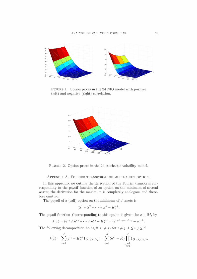
The option prices in these two cases are exhibited in Figure 1.Finally, in the stochastic volatility model we consider the parameters used

in Dempster and Hong (2002), that is S10 = 96, S2

0 = 100, σ1 = 0.5, σ2 = 1.0,σ3 = 0.05, ρ12 = 0.5, ρ13 = 0.25, ρ23 = −0.5, v0 = 0.04, κ = 1.0 andµ = 0.04; the option prices are shown in Figure 2.


85 90 95 100 105 110 115 0

0.5

10

1

2

3

4

5

6

7

8

9

10

8590

95100

105110

115 0

0.5

10

2

4

6

8

10

Figure 1. Option prices in the 2d NIG model with positive(left) and negative (right) correlation.

85 90 95 100 105 110 115 0

0.5

1

0

2

4

6

8

10

12

Figure 2. Option prices in the 2d stochastic volatility model.

Appendix A. Fourier transforms of multi-asset options

In this appendix we outline the derivation of the Fourier transform cor-responding to the payoff function of an option on the minimum of severalassets; the derivation for the maximum is completely analogous and there-fore omitted.

The payoff of a (call) option on the minimum of d assets is

(S1 ∧ S2 ∧ · · · ∧ Sd −K)+.

The payoff function f corresponding to this option is given, for x ∈ Rd, by

f(x) = (ex1 ∧ ex2 ∧ · · · ∧ exd −K)+ = (ex1∧x2∧···∧xd −K)+.

The following decomposition holds, if xi 6= xj for i 6= j, 1 ≤ i, j ≤ d

f(x) =

d∑

i=1

(exi −K)+1xi≤xj ,∀j =

d∑

i=1

(exi −K)

d∏

j=1j 6=i

1k<xi<xj,


where k = logK. Define also the auxiliary functions fi, 1 ≤ i ≤ d, where

fi(x) = (exi −K)

d∏

j=1j 6=i

1k<xi<xj.

The dampened payoff function is g(x) = e−〈R,x〉f(x), where R ∈ Rd;

we define analogously the dampened fi-functions, i.e. gi(x) = e−〈R,x〉fi(x).For simplicity, we first calculate the Fourier transform of the dampenedf1-function; for u ∈ Rd we get

g1(u) =

∫

Rd

e〈iu−R,x〉(ex1 −K)

d∏

j=2

1k<x1≤xjdx

=

∞∫

k

∞∫

x1

. . .

∞∫

x1

e〈iu−R,x〉(ex1 −K)dxd . . . dx1

=

∞∫

k

e(iu1−R1)x1(ex1 −K)

d∏

j=2

∞∫

x1

e(iuj−Rj)xjdxj

dx1

=

∞∫

k

e(iu1−R1)x1(ex1 −K)

d∏

j=2

(−e(iuj−Rj)x1

iuj −Rj

)dx1

=1

∏dj=2(Rj − iuj)

∞∫

k

ePd

j=1(iuj−Rj)x1(ex1 −K)dx1

=1

∏dj=2(Rj − iuj)

(− K1+

Pdj=1

(iuj−Rj)

1 +∑d

j=1(iuj −Rj)+K1+

Pdj=1

(iuj−Rj)

∑dj=1(iuj −Rj)

)

=K1+

Pdj=1

(iuj−Rj)

∏dj=2(Rj − iuj)×

(1 +

∑dj=1(iuj −Rj)

)×(∑d

j=1(iuj −Rj)) ,

subject to the conditions Rj > 0 for all j ≥ 2 and∑d

j=1Rj > 1.Hence, in general we have that

gl(u) =K1+

Pdj=1

(iuj−Rj)

∏dj=1j 6=l

(Rj − iuj)×(1 +

∑dj=1(iuj −Rj)

)×(∑d

j=1(iuj −Rj)) ,

subject to the conditions Rj > 0 for all 1 ≤ j ≤ d and∑d

j=1Rj > 1.


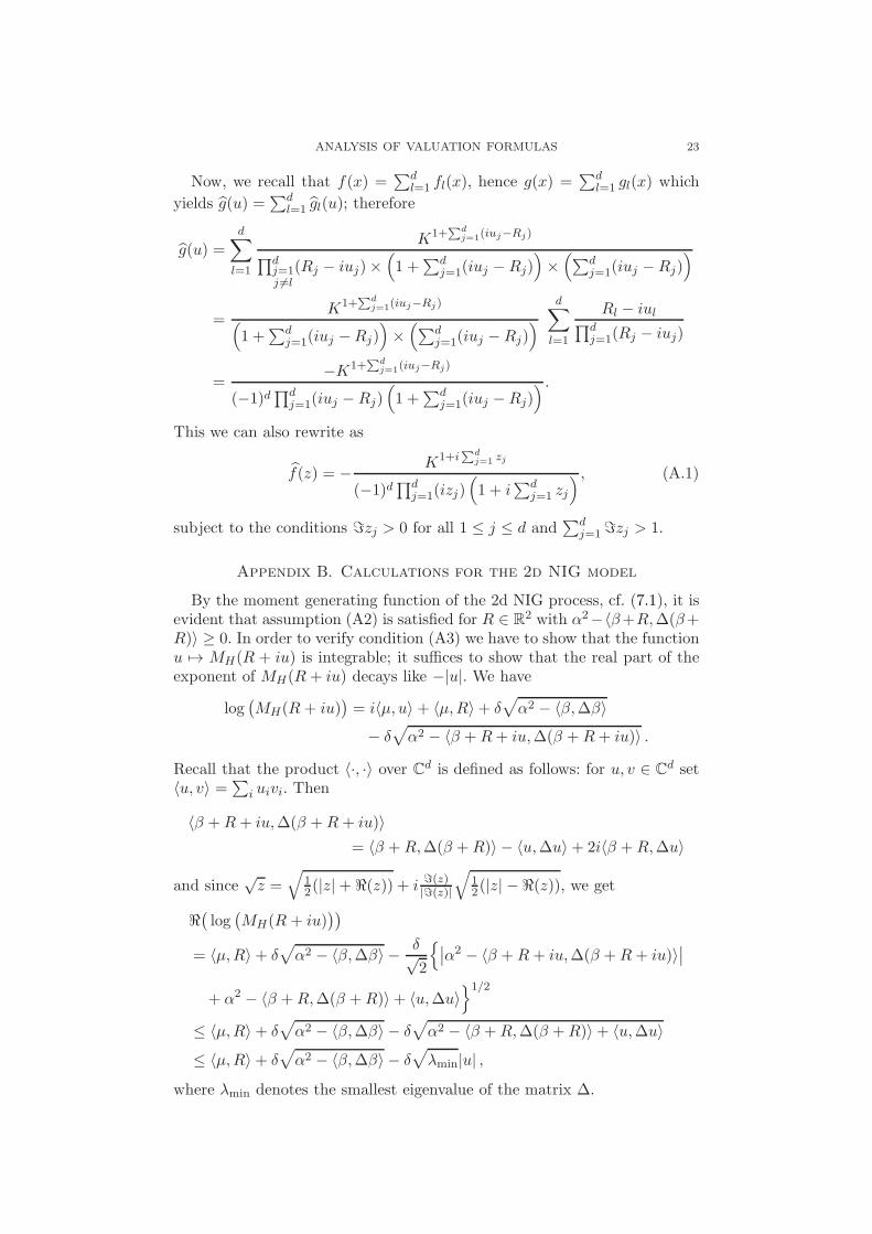
Now, we recall that f(x) =∑d

l=1 fl(x), hence g(x) =∑d

l=1 gl(x) which

yields g(u) =∑d

l=1 gl(u); therefore

g(u) =

d∑

l=1

K1+Pd

j=1(iuj−Rj)

∏dj=1j 6=l

(Rj − iuj)×(1 +

∑dj=1(iuj −Rj)

)×(∑d

j=1(iuj −Rj))

=K1+

Pdj=1

(iuj−Rj)

(1 +

∑dj=1(iuj −Rj)

)×(∑d

j=1(iuj −Rj))

d∑

l=1

Rl − iul∏dj=1(Rj − iuj)

=−K1+

Pdj=1

(iuj−Rj)

(−1)d∏d

j=1(iuj −Rj)(1 +

∑dj=1(iuj −Rj)

) .

This we can also rewrite as

f(z) = − K1+iPd

j=1zj

(−1)d∏d

j=1(izj)(1 + i

∑dj=1 zj

) , (A.1)

subject to the conditions ℑzj > 0 for all 1 ≤ j ≤ d and∑d

j=1ℑzj > 1.

Appendix B. Calculations for the 2d NIG model

By the moment generating function of the 2d NIG process, cf. (7.1), it isevident that assumption (A2) is satisfied for R ∈ R2 with α2−〈β+R,∆(β+R)〉 ≥ 0. In order to verify condition (A3) we have to show that the functionu 7→ MH(R + iu) is integrable; it suffices to show that the real part of theexponent of MH(R + iu) decays like −|u|. We have

log(MH(R + iu)

)= i〈µ, u〉 + 〈µ,R〉+ δ

√α2 − 〈β,∆β〉

− δ√α2 − 〈β +R+ iu,∆(β +R+ iu)〉 .

Recall that the product 〈·, ·〉 over Cd is defined as follows: for u, v ∈ Cd set〈u, v〉 =

∑i uivi. Then

〈β +R+ iu,∆(β +R+ iu)〉= 〈β +R,∆(β +R)〉 − 〈u,∆u〉+ 2i〈β +R,∆u〉

and since√z =

√12(|z|+ ℜ(z)) + i

ℑ(z)|ℑ(z)|

√12(|z| − ℜ(z)), we get

ℜ(log(MH(R + iu)

))

= 〈µ,R〉+ δ√α2 − 〈β,∆β〉 − δ√

2

∣∣α2 − 〈β +R+ iu,∆(β +R+ iu)〉∣∣

+ α2 − 〈β +R,∆(β +R)〉+ 〈u,∆u〉1/2

≤ 〈µ,R〉+ δ√α2 − 〈β,∆β〉 − δ

√α2 − 〈β +R,∆(β +R)〉+ 〈u,∆u〉

≤ 〈µ,R〉+ δ√α2 − 〈β,∆β〉 − δ

√λmin|u| ,

where λmin denotes the smallest eigenvalue of the matrix ∆.


References

Barndorff-Nielsen, O. E. (1998). Processes of normal inverse Gaussiantype. Finance Stoch. 2, 41–68.

Barndorff-Nielsen, O. E. and N. Shephard (2001). Non-GaussianOrnstein–Uhlenbeck-based models and some of their uses in financialeconomics. J. Roy. Statist. Soc. Ser. B 63, 167–241.

Biagini, F., Y. Bregman, and T. Meyer-Brandis (2008). Pricing of catas-trophe insurance options written on a loss index with reestimation.Insurance Math. Econom. 43, 214–222.

Blæsild, P. (1981). The two-dimensional hyperbolic distribution and re-lated distributions, with an application to Johannsen’s bean data.Biometrika 68, 251–263.

Bochner, S. (1955). Harmonic Analysis and the Theory of Probability.University of California Press.

Borovkov, K. and A. Novikov (2002). On a new approach to calculatingexpectations for option pricing. J. Appl. Probab. 39, 889–895.

Boyarchenko, S. I. and S. Z. Levendorskiı (2002). Non-Gaussian Merton-Black-Scholes Theory. World Scientific.

Breiman, L. (1968). Probability. Addison-Wesley Publishing Company.Carr, P., H. Geman, D. B. Madan, and M. Yor (2002). The fine structure

of asset returns: an empirical investigation. J. Business 75, 305–332.Carr, P., H. Geman, D. B. Madan, and M. Yor (2003). Stochastic volatility

for Levy processes. Math. Finance 13, 345–382.Carr, P. and D. B. Madan (1999). Option valuation using the fast Fourier

transform. J. Comput. Finance 2 (4), 61–73.Cont, R. and P. Tankov (2003). Financial Modelling with Jump Processes.

Chapman and Hall/CRC Press.Deitmar, A. (2004). A First Course in Harmonic Analysis (2nd ed.).

Springer.Dempster, M. A. H. and S. S. G. Hong (2002). Spread option valuation

and the fast Fourier transform. In Mathematical Finance – BachelierCongress 2000, pp. 203–220. Springer.

Doetsch, G. (1950). Handbuch der Laplace-Transformation. Birkhauser.Duffie, D., D. Filipovic, and W. Schachermayer (2003). Affine processes

and applications in finance. Ann. Appl. Probab. 13, 984–1053.Dufresne, D., J. Garrido, and M. Morales (2009). Fourier inversion for-

mulas in option pricing and insurance. Methodol. Comput. Appl.Probab. 11, 359–383.

Eberlein, E. (2001). Application of generalized hyperbolic Levy mo-tions to finance. In O. E. Barndorff-Nielsen, T. Mikosch, and S. I.Resnick (Eds.), Levy Processes: Theory and Applications, pp. 319–336.Birkhauser.

Eberlein, E., K. Glau, and A. Papapantoleon (2009). Analyticity of theWiener–Hopf factors and valuation of exotic options in Levy models.Working paper.

Eberlein, E. and U. Keller (1995). Hyperbolic distributions in finance.Bernoulli 1, 281–299.


Eberlein, E. and W. Kluge (2006a). Exact pricing formulae for caps andswaptions in a Levy term structure model. J. Comput. Finance 9 (2),99–125.

Eberlein, E. and W. Kluge (2006b). Valuation of floating range notes inLevy term structure models. Math. Finance 16, 237–254.

Eberlein, E. and W. Kluge (2007). Calibration of Levy term structuremodels. In M. Fu, R. A. Jarrow, J.-Y. Yen, and R. J. Elliott (Eds.),Advances in Mathematical Finance: In Honor of Dilip B. Madan, pp.155–180. Birkhauser.

Eberlein, E., W. Kluge, and P. J. Schonbucher (2006). The Levy Libormodel with default risk. J. Credit Risk 2, 3–42.

Eberlein, E. and N. Koval (2006). A cross-currency Levy market model.Quant. Finance 6, 465–480.

Eberlein, E., A. Papapantoleon, and A. N. Shiryaev (2008). On the dualityprinciple in option pricing: semimartingale setting. Finance Stoch. 12,265–292.

Eberlein, E., A. Papapantoleon, and A. N. Shiryaev (2009). Esscher trans-form and the duality principle for multidimensional semimartingales.Ann. Appl. Probab.. (forthcoming, arXiv/0809.0301).

Elstrodt, J. (1999). Maß- und Integrationstheorie (2nd ed.). Springer.Fournie, E., J.-M. Lasry, J. Lebuchoux, P.-L. Lions, and N. Touzi (1999).

Applications of Malliavin calculus to Monte Carlo methods in finance.Finance Stoch. 3, 391–412.

Heston, S. L. (1993). A closed-form solution for options with stochasticvolatility with applications to bond and currency options. Rev. Financ.Stud. 6, 327–343.

Heuser, H. (1993). Lehrbuch der Analysis I (10th ed.). Teubner.Hubalek, F. and J. Kallsen (2005). Variance-optimal hedging and

Markowitz-efficient portfolios for multivariate processes with station-ary independent increments with and without constraints. Workingpaper, TU Munchen.

Hubalek, F., J. Kallsen, and L. Krawczyk (2006). Variance-optimal hedg-ing for processes with stationary independent increments. Ann. Appl.Probab. 16, 853–885.

Hurd, T. R. and Z. Zhou (2009). A Fourier transform method for spreadoption pricing. Preprint, arXiv/0902.3643.

Jacod, J. and A. N. Shiryaev (2003). Limit Theorems for Stochastic Pro-cesses (2nd ed.). Springer.

Kallsen, J. (2006). A didactic note on affine stochastic volatility models.In Y. Kabanov, R. Lipster, and J. Stoyanov (Eds.), From StochasticCalculus to Mathematical Finance: The Shiryaev Festschrift, pp. 343–368. Springer.

Katznelson, Y. (2004). An Introduction to Harmonic Analysis (Third ed.).Cambridge University Press.

Keller-Ressel, M. (2008). Affine processes – theory and applications tofinance. Ph. D. thesis, TU Vienna.

Keller-Ressel, M., A. Papapantoleon, and J. Teichmann (2009). A newapproach to LIBOR modeling. Preprint, arXiv/0904.0555.


Kilin, F. (2007). Accelerating the calibration of stochastic volatility mod-els. Working paper, HfB.

Kohatsu-Higa, A. and K. Yasuda (2009). A review of some recent resultsof Malliavin Calculus and its applications. Radon Ser. Comput. Appl.Math. (forthcoming).

Lee, R. W. (2004). Option pricing by transform methods: extensions, uni-fication, and error control. J. Comput. Finance 7 (3), 50–86.

Lord, R. (2008). Efficient pricing algorithms for exotic derivatives. Ph. D.thesis, Univ. Rotterdam.

Madan, D. B. and E. Seneta (1990). The variance gamma (VG) model forshare market returns. J. Business 63, 511–524.

Nicolato, E. and E. Venardos (2003). Option pricing in stochastic volatilitymodels of the Ornstein–Uhlenbeck type. Math. Finance 13, 445–466.

Papapantoleon, A. (2007). Applications of semimartingales and Levy pro-cesses in finance: duality and valuation. Ph. D. thesis, Univ. Freiburg.

Pinsky, M. A. (1993). Fourier inversion for piecewise smooth functions inseveral variables. Proc. Amer. Math. Soc. 118, 903–910.

Prause, K. (1999). The generalized hyperbolic model: estimation, financialderivatives, and risk measures. Ph. D. thesis, Univ. Freiburg.

Raible, S. (2000). Levy processes in finance: theory, numerics, and empir-ical facts. Ph. D. thesis, Univ. Freiburg.

Rudin, W. (1987). Real and Complex Analysis (3rd ed.). McGraw-Hill.Sato, K. (1999). Levy Processes and Infinitely Divisible Distributions.

Cambridge University Press.Sauvigny, F. (2006). Partial Differential Equations 2. Springer.Schoutens, W. (2003). Levy Processes in Finance: Pricing Financial

Derivatives. Wiley.Schoutens, W. and J. L. Teugels (1998). Levy processes, polynomials and

martingales. Comm. Statist. Stochastic Models 14, 335–349.Stein, E. M. and G. Weiss (1971). Introduction to Fourier Analysis on

Euclidean Spaces. Princeton University Press.Teichmann, J. (2006). Calculating the Greeks by cubature formulae. Proc.

R. Soc. Lond. A 462, 647–670.Zimmer, R. J. (1990). Essential Results of Functional Analysis. University

of Chicago Press.

Department of Mathematical Stochastics, University of Freiburg, Ecker-

str. 1, 79104 Freiburg, Germany

E-mail address: [email protected]

Department of Mathematical Stochastics, University of Freiburg, Ecker-

str. 1, 79104 Freiburg, Germany


Institute of Mathematics, TU Berlin, Straße des 17. Juni 136, 10623 Berlin,

Germany & Quantitative Products Laboratory, Deutsche Bank AG, Alexan-

derstr. 5, 10178 Berlin, Germany


Documents

ANALYSIS OF FOURIER TRANSFORM VALUATION FORMULAS AND ... · ANALYSIS OF FOURIER TRANSFORM VALUATION FORMULAS AND APPLICATIONS ERNST EBERLEIN, KATHRIN GLAU, AND ANTONIS PAPAPANTOLEON