Embed Size (px)
Citation preview

© SEP 2019 | IRE Journals | Volume 3 Issue 3 | ISSN: 2456-8880
IRE 1701668 ICONIC RESEARCH AND ENGINEERING JOURNALS 142
Analysis of Fault Detection Algorithm for Power System
Transmission Lines Using DFT and FFT
OGBOH V. C1, EZECHUKWU O. A
2, MADUEME T. C.
3
Department of Electrical Engineering Nnamdi Azikiwe University, Awka, Nigeria
Abstract- the Development of Fault Detection
Algorithm for power system transmission line
consists of two algorithms. Discrete Fourier
Transform (DFT) and Fast Fourier Transform
(FFT). A block diagram is developed which shows
the developmental stages of the algorithms. The
DFT and FFT detection algorithms are developed
based on their individual applications of Fourier
Transform (FT) discretization of phase values of
voltage and current to obtain the discrete versions
(VP and IP) as the required data for the research.
The discretization is followed by DFT and FFT
applications to the output result (VP and IP) of the
discretization to obtain the time – domain and
frequency – domain components. Mathematical
approach of the implementation of the algorithm is
performed and the values of the phase discrete
voltage and current values, pre-fault and three
phase fault voltage and current magnitudes for
DFT and FFT applications were obtained and
tabulated.
Indexed Terms- DFT, FFT, Algorithm, Voltage,
Current, impedance, Transmission Line, Faults,
Matlab, Simulink
I. INTRODUCTION
There has been rapid growth of the power grids all
over the world in the past decades. This growth has
led to the installation of large number of new
transmission and distribution lines to ensure
provision of sufficient power supply to end user.
Moreover, the continuity of this power supply is
highly important, this is because, and insufficient
power supply can cause a lot of problems or set -
back to the country. The problem can be summarized
as decrease in economy and infrastructural
development of that country.
One of the factors which can cause discontinuity of
this power supply from reaching the end users is
faults (Balance or Unbalanced faults).
Therefore, the fault developed or occurred on the
power system transmission line must be cleared as
fast as possible to enable the isolated part of the
transmission line due to fault receive power supply
and to prevent further damage of the power system
equipment or cause black – out in the country.
Various methods have been employed for detecting,
classifying, locating and analyzing these faults. They
include; Impedance measurement based method
Travelling wave based method Signal processing
based method (Discrete Fourier Transform (DFT),
Fast Fourier Transform (FFT), Wavelet (WT) and S-
Transform (ST) Artificial Intelligent system (AI)
based method etc.
II. METHODOLOGY
Methodological procedure followed in this research
is shown on figure 1. The Modeling of the power
system transmission line shown in figure 2 is done
using Matlab/Simulink 2016a and Onitsha
transmission station parameters, such as Real Power
87.7MW, Reactive Power 21.40MVAR, and Active
Power of 90.27MVA with frequency of 50Hz and
line distance of 96km from Onitsha to Enugu. The
modeled transmission line is shown on figure 4.
Mathematical Approach for DFT: The
mathematical expressions for DFT is employed
using the sampled three phase voltage and current
signals (v (t) and i (t)) as inputs of the DFT
algorithm. In this mathematical approach, three
phase sets of samples or data of v(t) and i(t) each
are used with number of samples N equals to
three (3). Two types of samples are used, the pre-
fault and faulted samples. Table 1 and 2 shows

© SEP 2019 | IRE Journals | Volume 3 Issue 3 | ISSN: 2456-8880
IRE 1701668 ICONIC RESEARCH AND ENGINEERING JOURNALS 143
both type of samples assumed to have been
obtained through equations 2.1 to 2.6.
Va = Vpa sin (Ѳ ± Ø) 2.1
Vb = Vpb sin (Ѳ ± Ø) 2.2
Vc = Vpc sin (Ѳ ± Ø) 2.3
Ia = Ipa sin (Ѳ ± ψ) 2.4
Ib = Ipb sin (Ѳ ± ψ) 2.5
Ic = Ipc sin (Ѳ ± ψ) 2.6
Figure 1: Block diagram of the procedure
Figure 2: 330/132KV transmission line representing
Onitsha – Enugu
2.7
2.8
2.9
2.10
2.11
2.12
Equations 2.7 and 2.8 are phase voltage and current
discretizing equations respectively. Equation 2.9 and
2.10 is used to obtain the actual voltage and current
complex or composite signals respectively. However
equations 2.11 and 2.12 are used to compute the DFT
voltage and current values.
The DFT of a signal v(t) or i(t) is given as Equations
2.11 and 2.12 respectively. Where, Vx(n) or Ix(n) is
the DFT of the sequence v(n), or I(n) and using v(n)
and I(n) equal to;
V(n) = [v(0), v(1), v(2), v(3)]T and I(n) = [I(0), I(1),
I(2), I(3)]T respectively for 4 – point DFT application
having
N = 4 (number of DFT samples).
V (n) can be represented in matrix form as follows:
Where
W = exp ((-J2π)/ (N)) and W = W2N
= 1 2.13
For a 4 – point DFT application, where N = 4
Thus,
W = exp ((-J2π)/ (N)) = exp ((-J2π)/ (4))
= exp ((-Jπ)/ (2)) = a
2.14
a2 = -j, 2.15
a3 = -ja = -a* 2.16
a4 = -1 2.17
Therefore, the DFT of the voltage and current signals
for any condition is given by equation 2.18
2.18
2.19
Thus,
© SEP 2019 | IRE Journals | Volume 3 Issue 3 | ISSN: 2456-8880
IRE 1701668 ICONIC RESEARCH AND ENGINEERING JOURNALS 144
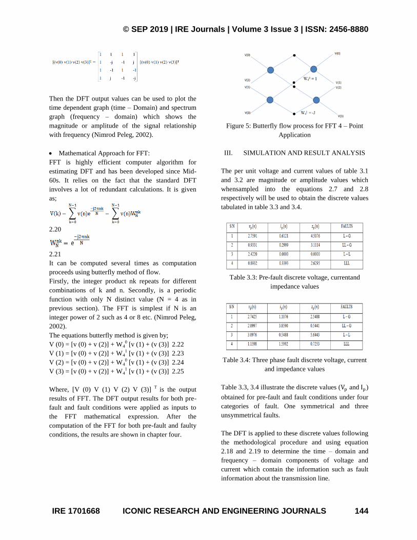
Then the DFT output values can be used to plot the
time dependent graph (time – Domain) and spectrum
graph (frequency – domain) which shows the
magnitude or amplitude of the signal relationship
with frequency (Nimrod Peleg, 2002).
Mathematical Approach for FFT:
FFT is highly efficient computer algorithm for
estimating DFT and has been developed since Mid-
60s. It relies on the fact that the standard DFT
involves a lot of redundant calculations. It is given
as;
2.20
2.21
It can be computed several times as computation
proceeds using butterfly method of flow.
Firstly, the integer product nk repeats for different
combinations of k and n. Secondly, is a periodic
function with only N distinct value (N = 4 as in
previous section). The FFT is simplest if N is an
integer power of 2 such as 4 or 8 etc. (Nimrod Peleg,
2002).
The equations butterfly method is given by;
V (0) = [v (0) + v (2)] + W40 [v (1) + (v (3)] 2.22
V (1) = [v (0) + v (2)] + W41 [v (1) + (v (3)] 2.23
V (2) = [v (0) + v (2)] + W40 [v (1) + (v (3)] 2.24
V (3) = [v (0) + v (2)] + W41 [v (1) + (v (3)] 2.25
Where, [V (0) V (1) V (2) V (3)] T
is the output
results of FFT. The DFT output results for both pre-
fault and fault conditions were applied as inputs to
the FFT mathematical expression. After the
computation of the FFT for both pre-fault and faulty
conditions, the results are shown in chapter four.
Figure 5: Butterfly flow process for FFT 4 – Point
Application
III. SIMULATION AND RESULT ANALYSIS
The per unit voltage and current values of table 3.1
and 3.2 are magnitude or amplitude values which
whensampled into the equations 2.7 and 2.8
respectively will be used to obtain the discrete values
tabulated in table 3.3 and 3.4.
Table 3.3: Pre-fault discrete voltage, currentand
impedance values
Table 3.4: Three phase fault discrete voltage, current
and impedance values
Table 3.3, 3.4 illustrate the discrete values (Vp and Ip)
obtained for pre-fault and fault conditions under four
categories of fault. One symmetrical and three
unsymmetrical faults.
The DFT is applied to these discrete values following
the methodological procedure and using equation
2.18 and 2.19 to determine the time – domain and
frequency – domain components of voltage and
current which contain the information such as fault
information about the transmission line.

© SEP 2019 | IRE Journals | Volume 3 Issue 3 | ISSN: 2456-8880
IRE 1701668 ICONIC RESEARCH AND ENGINEERING JOURNALS 145
Table 3.5: Mathematical Approach DFT Application
for Pre-fault Condition at N – POINTS(k = 0… N –
1)
Table 3.6: Mathematical Approach DFT Application
for Three Phase Fault Condition at N – POINTS (k =
0… N – 1)
Table 3.7: Mathematical Approach FFT Application
for Pre-fault Condition at N – POINTS (k = 0… N –
1)
Table 3.8: Mathematical Approach FFT
Applicationfor Three Phase Fault Condition at N –
POINTS(k = 0…, N – 1)
The DFT and FFT results obtained using
mathematical approach are tabulated on table 3.5 &
3.6 and table 3.7 & 3.8 for three phase (LLL) pre-
fault and fault conditions respectively.
To obtain the time – domain and frequency – domain
waveform and spectrum diagram representing V(n),
I(n) and V(k), I(k) respectively, we plot V(n) and I(n)
individually against time for time domain and against
the frequency for frequency domain (spectrum
waveform) using Matlab.
Figure 3.1: Mathematical Approach Pre-Fault DFT
Voltage (Vn) t - domain Signal Waveform
Figure 3.2: Mathematical Approach Pre-Fault DFT
Voltage (Vn) s – domain Signal Waveform
Figure 3.1 and 3.2 are the time and frequency –
domain pre-fault DFT voltage signal waveform
obtained by plotting the Vn against time t and
frequency respectively. The waveform is not
sinusoidal even at No fault condition. It also shows
that the maximum amplitude of Vn is 13.8pu at time
of 2secs and largest magnitude of 275pu at 0.48Hz.

© SEP 2019 | IRE Journals | Volume 3 Issue 3 | ISSN: 2456-8880
IRE 1701668 ICONIC RESEARCH AND ENGINEERING JOURNALS 146
Figure 3.3: Mathematical Approach Pre-Fault DFT
Current (In) t – domain Signal Waveform
Figure 3.4: Mathematical Approach Pre-Fault DFT
Current (In) s – domain Signal Waveform
Figure 3.3 and 3.4 are the time and frequency –
domain pre-fault DFT current signal waveform
obtained by plotting the In against time t and
frequency respectively. The waveform is not
sinusoidal even at No fault condition. It also shows
that the maximum amplitude of In is 0.6pu at time of
2secs and largest magnitude of 11pu at 0.25Hz.
Figure 3.5: Mathematical Approach Three Phase
Fault DFT Voltage (Vn) t – domain Signal
Waveform
Figure 3.6: Mathematical Approach Three Phase
Fault DFT Voltage (Vn) s – domain Signal
Waveform
Figure 3.5 and 3.6 are the time and frequency domain
three phase fault DFT voltage signal waveform
obtained by plotting the Vn against time t and
frequency respectively. The waveform is under three
phase fault condition. It also shows that the
maximum amplitude of Vn is 2pu at time of 2secs and
largest magnitude of 35pu at 0.25Hz
Figure 3.7: Mathematical Approach Three Phase
Fault DFT Current (In) t – domain Signal Waveform
© SEP 2019 | IRE Journals | Volume 3 Issue 3 | ISSN: 2456-8880
IRE 1701668 ICONIC RESEARCH AND ENGINEERING JOURNALS 147
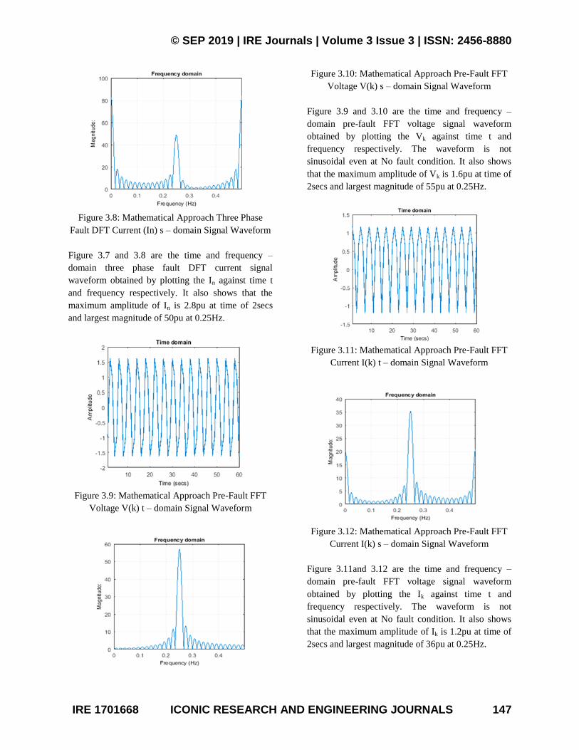
Figure 3.8: Mathematical Approach Three Phase
Fault DFT Current (In) s – domain Signal Waveform
Figure 3.7 and 3.8 are the time and frequency –
domain three phase fault DFT current signal
waveform obtained by plotting the In against time t
and frequency respectively. It also shows that the
maximum amplitude of In is 2.8pu at time of 2secs
and largest magnitude of 50pu at 0.25Hz.
Figure 3.9: Mathematical Approach Pre-Fault FFT
Voltage V(k) t – domain Signal Waveform
Figure 3.10: Mathematical Approach Pre-Fault FFT
Voltage V(k) s – domain Signal Waveform
Figure 3.9 and 3.10 are the time and frequency –
domain pre-fault FFT voltage signal waveform
obtained by plotting the Vk against time t and
frequency respectively. The waveform is not
sinusoidal even at No fault condition. It also shows
that the maximum amplitude of Vk is 1.6pu at time of
2secs and largest magnitude of 55pu at 0.25Hz.
Figure 3.11: Mathematical Approach Pre-Fault FFT
Current I(k) t – domain Signal Waveform
Figure 3.12: Mathematical Approach Pre-Fault FFT
Current I(k) s – domain Signal Waveform
Figure 3.11and 3.12 are the time and frequency –
domain pre-fault FFT voltage signal waveform
obtained by plotting the Ik against time t and
frequency respectively. The waveform is not
sinusoidal even at No fault condition. It also shows
that the maximum amplitude of Ik is 1.2pu at time of
2secs and largest magnitude of 36pu at 0.25Hz.

© SEP 2019 | IRE Journals | Volume 3 Issue 3 | ISSN: 2456-8880
IRE 1701668 ICONIC RESEARCH AND ENGINEERING JOURNALS 148
Figure 3.13: Mathematical Approach Three Phase
Fault FFT Voltage (Vk) t – domain Signal Waveform
Figure 3.14: Mathematical Approach Three Phase
Fault FFT Voltage (Vk) s – domain Signal Waveform
Figure 3.13 and 3.14 are the time and frequency –
domain three phase fault FFT voltage signal
waveform obtained by plotting the Vk against time t
and frequency respectively. The waveform is under
three phase fault condition. It also shows that the
maximum amplitude of Vk is 1.7pu at time of 2secs
and largest magnitude of 35pu at 0.25Hz.
Figure 3.15: Mathematical Approach Three Phase
Fault FFT Current I(k) t – domain Signal Waveform
Figure 3.16: Mathematical Approach Three Phase
Fault FFT Current I(k) s – domain Signal Waveform
Figure 3.15 and 3.16 are the time and frequency –
domain three phase fault FFT current signal
waveform obtained by plotting the IK against time t
and frequency respectively. It also shows that the
maximum amplitude of IK is 2.2pu at time of 2secs
and largest magnitude of 10pu at 0.25Hz.
Figure 3.17: Mathematical Approach DFT Pre-
faultand Three Phase fault Voltages
Figure 3.17 show that pre-fault voltage is higher than
that of three phase fault by 10.8pu. This is because of
the occurrence of fault.
Figure 3.18: Mathematical Approach DFTPre-fault
and Three Phase fault Currents
© SEP 2019 | IRE Journals | Volume 3 Issue 3 | ISSN: 2456-8880
IRE 1701668 ICONIC RESEARCH AND ENGINEERING JOURNALS 149
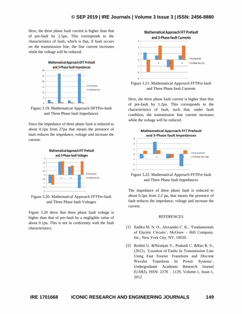
Here, the three phase fault current is higher than that
of pre-fault by 2.5pu. This corresponds to the
characteristics of fault, which is that, if fault occurs
on the transmission line, the line current increases
while the voltage will be reduced.
Figure 3.19: Mathematical Approach DFTPre-fault
and Three Phase fault Impedances
Since the impedance of three phase fault is reduced to
about 0.1pu from 27pu that means the presence of
fault reduces the impedance, voltage and increase the
current.
Figure 3.20: Mathematical Approach FFTPre-fault
and Three Phase fault Voltages
Figure 3.20 show that three phase fault voltage is
higher than that of pre-fault by a negligible value of
about 0.1pu. This is not in conformity with the fault
characteristics.
Figure 3.21: Mathematical Approach FFTPre-fault
and Three Phase fault Currents
Here, the three phase fault current is higher than that
of pre-fault by 1.2pu. This corresponds to the
characteristics of fault, such that, under fault
condition, the transmission line current increases
while the voltage will be reduced.
Figure 3.22: Mathematical Approach FFTPre-fault
and Three Phase fault Impedances
The impedance of three phase fault is reduced to
about 0.5pu from 2.2 pu, that means the presence of
fault reduces the impedance, voltage and increase the
current.
REFERENCES
[1] Sadiku M. N. O., Alexander C. K., ‘Fundamentals
of Electric Circuits’, McGraw – Hill Company.
Inc., New York City, NY, 10020.
[2] Roshni U. &Niranjan V., Prakash C. &Rao R. S.,
(2012), ‘Location of Faults In Transmission Line
Using Fast Fourier Transform and Discrete
Wavelet Transform In Power Systems’,
Undergraduate Academic Research Journal
(UARJ), ISSN: 2278 – 1129, Volume-1, Issue-1,
2012
© SEP 2019 | IRE Journals | Volume 3 Issue 3 | ISSN: 2456-8880
IRE 1701668 ICONIC RESEARCH AND ENGINEERING JOURNALS 150
[3] Mamis M. S., Arkan M., (2011), ‘FFT Based
Fault Location Algorithm for Transmission Lines’
[4] Robi P., 2013. ‘Tutorial on Signal Analysis
Method of Fault Study’
[5] Ashrafian A., Rostani M., Gharehpetian G. B.,
Gholamphasemi M., 2012. ‘Application of
Discrete S – Transform for Differential Protection
of Power Transformer’. International Journal of
Computer and Electrical Engineering, Vol. 4, No
2, April 2012.


![Enhance High Impedance Fault Detection and …yweng2/papers/2019TSG-PMU.pdfalgorithm [2], impedance-based method [3] and PC-based fault locating and diagnosis algorithm [4], etc. However,](https://img.dokumen.tips/doc/110x75/5fe122d4df236711b2274e10/enhance-high-impedance-fault-detection-and-yweng2papers2019tsg-pmupdf-algorithm.jpg)