Embed Size (px)
Citation preview

Analysis of Electric Disturbances from the Static
Frequency Converter of a Pumped Storage Station
Sebastian P. Rosado
Thesis submitted to the Faculty of the Virginia Polytechnic Institute and State
University in partial fulfillment of the requirements for the degree of
Master of Science
in
Electrical Engineering
Dr. Yilu Liu, Chair
Dr. Arun G. Phadke
Dr. Jaime de la Ree Lopez
August 9, 2001
Blacksburg, Virginia
Keywords: power quality, power system transients, power system harmonics, power
transformers, synchronous machines, variable speed drives, frequency conversion, power
system modeling

ii
Analysis of Electric Disturbances from the Static Frequency
Converter of a Pumped Storage Station
Sebastian P. Rosado
Abstract
The present work studies the disturbances created in the electric system of a pumped
storage power plant, which is an hydraulic generation facility where the machines can work
as turbines or pumps, by the operation of a static frequency converter (SFC). The SFC is used
for starting the synchronous machines at the station when in the pump mode. During the
starting process several equipment is connected to the SFC being possible to get affected by
the disturbances generated. These disturbances mainly include the creation of transient
overvoltages during the commutation of the semiconductor devices of the SFC and the
introduction of harmonics in the network currents and voltages. This work analyzes the
possible effects of the SFC operation over the station equipment based on computer
simulations. For this purpose, the complete system was modeled and the starting process
simulated in a computer transient simulator program. The work begins with a general review
of the effects of electric disturbances over high voltage equipment and in particular of the
disturbances generated by power electronics conversion equipment. Then the models for the
different kind of equipment present in the system are discussed and formulated. The control
system that governs the operation of the SFC during the starting process is analyzed later as
well as the operation conditions. Once the model of the system is set up, the harmonic
analysis of the electric network is done by frequency domain and time domain methods.
Time domain methods are also employed for the analysis of the commutation transient
produced by the SFC operation. Finally, the simulation results are used to evaluate the impact
of the SFC operation on the station equipment, especially on the generator step up
transformer.

iii
Acknowledgments
There are too many people that helped me in one way or another to complete my
Masters. In the department of Electrical Engineering at Virginia Tech I would like to thank
everyone in the center for power engineering, especially my advisor Dr. Yilu Liu for her
guidance during this two years. Thanks also to the other members of my committee Dr. Arun
Phadke and Dr. Jaime de la Ree for the knowledge shared during this time, Dr. Virgilio
Centeno and my lab partners for many useful technical (or not) discussions and their
friendship, and Dr. Xuzhu Dong for his help during the development of part of this work. I
am also grateful to the Fulbright Commission and the Organization of American States for
sponsoring my master studies.
Most of all I would like to thank all my family, especially my parents for their
unconditional support. And thanks God for allowing me reach this goal.

iv
Table of Contents
Acknowledgments .................................................................................................................. iii
Table of Contents ................................................................................................................... iv
1 Introduction..................................................................................................................... 1
1.1 Object of the Study ................................................................................................... 1
1.2 Description of the Facility under study..................................................................... 2
2 Effects of Disturbances on the Electric Equipment ..................................................... 5
2.1 Temporary Overvoltages and Overcurrents .............................................................. 6
2.2 Switching Transients - Very Fast Transients ............................................................ 6
2.3 Lightning................................................................................................................... 8
2.4 Waveform Distortion ................................................................................................ 9
3 Disturbances Generated by Power Electronics Conversion Equipment ................. 11
3.1 Commutation Transients......................................................................................... 11
3.2 Resonance at Harmonic Frequencies ...................................................................... 13
3.3 Overheating in Power Transformers due to Harmonics ......................................... 14
3.4 Transformer derating, K factor and other non-sine wave evaluation factors.......... 17
3.5 Transformer loss of life due to harmonic effects .................................................... 19
4 Modeling of the System ................................................................................................ 21
4.1 Supply Network and Starting Transformer ............................................................. 21
4.2 The Synchronous Machine ...................................................................................... 22
4.2.1 General considerations about machine modeling ........................................... 22
4.2.2 Computer model of the Synchronous machine ............................................... 25
4.3 The Static Frequency Converter ............................................................................. 27
4.3.1 General considerations of the SFC modeling ................................................. 27
4.3.2 Parameters of the computer model of the SFC ............................................... 31
4.4 GSU Transformer.................................................................................................... 32
4.5 Transmission Cable................................................................................................. 36
5 Control Strategy of the Static Frequency Converter................................................. 39
5.1 Inverter Control....................................................................................................... 41

v
5.2 Rectifier Control ..................................................................................................... 44
5.3 Forced Commutation Stage ..................................................................................... 45
6 Operation Conditions ................................................................................................... 47
7 Harmonic Analysis of the System................................................................................ 49
7.1 Frequency Domain Methodologies for Harmonic Analysis ................................... 49
7.2 Frequency Scan of the System Components........................................................... 52
7.2.1 Cable Frequency Scan..................................................................................... 53
7.2.2 Cable and Transformer Frequency Scan......................................................... 54
7.3 Frequency Scan of the Starting System .................................................................. 55
7.4 Analysis of Frequency Scan Results ....................................................................... 57
8 Time Domain Simulation ............................................................................................. 58
8.1 Rated Operating Conditions (Base case) ................................................................ 59
8.2 Other Operating Conditions at Natural Commutation............................................ 66
8.2.1 Effect of the load current on the circuit behavior ........................................... 66
8.2.2 Effect of the system speed on the circuit magnitudes ..................................... 68
8.2.3 Effect of the transmission cable on the circuit behavior ................................. 71
8.3 Operation at Forced Commutation.......................................................................... 74
8.4 Analysis of the Commutation Transient ................................................................. 77
8.5 Validation of the Simulation Results ...................................................................... 83
9 Analysis of the Results .................................................................................................. 85
9.1 Harmonics ............................................................................................................... 85
9.2 Overheating effects ................................................................................................. 86
9.3 Commutation Transients......................................................................................... 88
10 Conclusions .................................................................................................................... 89
Appendix A ............................................................................................................................ 90
A.1 Synchronous Machine Data .................................................................................... 90
A.2 Transmission Cable Data ........................................................................................ 91
A.3 SFC Control Circuit Diagram ................................................................................. 92
A.4 SFC Power Circuit Diagram ................................................................................... 95
Appendix B ............................................................................................................................ 97
B.1 Rated operating conditions –base case.................................................................... 97

vi
B.2 Reduced load condition......................................................................................... 102
B.3 Reduced Speed condition, ω=0.5*ωr .................................................................... 104
B.4 Operation without HV transmission cable ............................................................ 106
B.5 Forced Commutation Mode .................................................................................. 108
B.6 Snubber circuit not operative ................................................................................ 111
B.7 Snubber Circuit Operative .................................................................................... 112
B.7.1 Natural Commutation.................................................................................... 112
B.7.2 Forced Commutation..................................................................................... 113
B.8 Failure in the Firing Sequence .............................................................................. 114
References............................................................................................................................ 115
Vita ....................................................................................................................................... 119

vii
List of Illustrations Figure 1.1. Simplified on- line diagram of the pumped storage generation station used
during this study.................................................................................................................3
Figure 2.1 Voltage ratio between one step of a tapped winding and the whole HV
winding vs. frequency (taken from [5]) .............................................................................8
Figure 3.1 relevant parameters in the study of the effects of a transient waveform................13
Figure 3.2 Equivalent circuit of a two winding transformer....................................................14
Figure 4.1 PSCAD/EMTDC model of the auxiliary network and starting transformer ..........22
Figure 4.2 Electromagnetic circuit model of the synchronous machine..................................23
Figure 4.3 Equivalent circuit model of the synchronous machine ...........................................25
Figure 4.4 Circuit model of the static frequency converter .....................................................27
Figure 4.5 Voltage and current waveforms of SFC on the AC output side .............................29
Figure 4.6 Circuit model of the inverter side of the static frequency converter and the
synchronous machine .......................................................................................................31
Figure 4.7 Thyristor and snubber circuit..................................................................................31
Figure 4.8 Single-phase transformer model.............................................................................33
Figure 4.9 Simplified magnetizing curve .................................................................................35
Figure 4.10 Equivalent circuit of the frequency dependent line model...................................36
Figure 4.11 Frequency dependence of the cable surge impedance..........................................38
Figure 5.1 Curve of the speed evolution for the SFC starting of a synchronous
machine in the facility under study [39] ..........................................................................40
Figure 5.2 Circuit model of the static frequency converter .....................................................41
Figure 5.3 Commutation process of a semiconductor in the SFC inverter..............................42
Figure 5.4 Phasor diagram of the synchronous machine voltages and fluxes .........................43
Figure 5.5 Block diagram of the inverter control circuit .........................................................43
Figure 5.6 Block diagram of the control system of the SFC rectifier ......................................44
Figure 5.7 Three-phase current waveforms and forced commutation sequence in the
inverter bridge ..................................................................................................................46
Figure 6.1 Schematic of the SFC starting system....................................................................47
Figure 7.1 Generic electrical network......................................................................................50

viii
Figure 7.2 Circuit for cable frequency scan showing the variable frequency source,
cable and different meters................................................................................................52
Figure 7.3 Result of the frequency scan for the cable model. Although our main
interest and model validity is on the 0-20 kHz range, the scan covers up to 200
kHz. It is observed a series resonant frequency of the EMTDC model at 81 kHz..........53
Figure 7.4 Result of the frequency scan for the cable model on the low frequency
range.................................................................................................................................54
Figure 7.5 Result of the low frequency scan for the cable and transformer ............................55
Figure 7.6 Frequency scan circuit for the cable, transformer and generator group .................56
Figure 7.7 Frequency response of the cable, generator and transformer group .......................56
Figure 8.1 Vtab Line –line voltage at the transformer HV terminal. As the cable is not
loaded it is very close to the voltage at the cable open-end .............................................60
Figure 8.2 Vab Line – line voltage at the SFC converter output side, 16.5 kV.......................61
Figure 8.3 Vsab Line –line voltage at the converter input side, 16.5kV.................................61
Figure 8.4 Vna Line –ground voltage at the auxiliary bus if the station, 13.8 kV. ..................62
Figure 8.5 Iatr Phase current at the LV winding of the main transformer, in the delta
winding.............................................................................................................................63
Figure 8.6 Iag Synchronous machine input current .................................................................64
Figure 8.7 Iato SFC output current. There is no major difference with Isa2, the input
current of the SFC............................................................................................................64
Figure 8.8 Isa SFC input current at the primary side of the auxiliary transformer,
13.8kV..............................................................................................................................65
Figure 8.9 Vtab, line –line voltage at the transformer HV terminal. The harmonic
content is reduced respect to the base case ......................................................................67
Figure 8.10 Vab, line – line voltage at the SFC output (the machine side) .............................67
Figure 8.11 Iat, line current at the LV side of the main transformer .......................................68
Figure 8.12 Vtab Line to line voltage at the high voltage side of the GSU transformer .........69
Figure 8.13 Vtab Line to line voltage at the high voltage side of the GSU transformer .........70
Figure 8.14 Iatr Current at the transformer LV winding .........................................................70
Figure 8.15 SFC currents (a) at the SFC input the frequency is 60Hz (b) at the SFC
output, f=30Hz.................................................................................................................71

ix
Figure 8.16 Vtab Line –line voltage at the transformer HV terminal......................................72
Figure 8.17 Iatr Current at the LV winding of the main transformer, inside the
triangle connection...........................................................................................................73
Figure 8.18 Iag current taken by the synchronous machine ....................................................73
Figure 8.19 Irect Current at the DC interface between the rectifier and inverter ....................74
Figure 8.20 Isa2 Line current at AC three phase input of the SFC, at 16.5 KV......................75
Figure 8.21 Et3 Voltage at terminals of a GTO in the inverter bridge ....................................75
Figure 8.22 Vtab Line to line voltage at the GSU transformer HV winding...........................76
Figure 8.23 Iatr current at the LV winding of the GSU transformer .......................................77
Figure 8.24 Line to line voltage at the SFC input 16.5 KV.....................................................79
Figure 8.25 Line to ground voltage at the SFC input 16.5 KV................................................79
Figure 8.26 Line to ground voltage at the SFC machine side, 16.5 KV a small
commutation disturbance is observed ..............................................................................80
Figure 8.27 Line to ground voltage at the transformer HV side 345 KV, at rated
frequency..........................................................................................................................80
Figure 8.28 Voltage in the DC current loop during normal operation (forced), the
negative spikes correspond to instants where current is cancelled ..................................81
Figure 8.29 Vab voltage at the SFC machine side; (a) waveform with the spikes at
current interruption (b) detail of a spike, the peak is limited by the surge arrester
operation...........................................................................................................................82
Figure 8.30 Vta phase to ground voltage at the transformer HV side, forced
commutation, failure in GTO triggering ..........................................................................82
Figure A.1 Transmission Cable model ....................................................................................91
Figure A.2 SFC Control circuit: Rectifier control ...................................................................92
Figure A.3 SFC Control circuit: Rectifier-Inverter control circuits ........................................93
Figure A.4 SFC Control Circuit: Inverter control....................................................................94
Figure A.5 SFC Power Circuit: this portion shows the SFC itself and the auxiliary
source ...............................................................................................................................95
Figure A.6 SFC Power Circuit: this portion shows the synchronous machine, GSU
transformer, and HV cable ...............................................................................................96
Figure B.1 Voltage waveforms at rated conditions at the transformer HV terminals .............97

x
Figure B.2 Voltage waveforms at rated operating condition...................................................98
Figure B.3 Voltage waveforms at rated operating conditions .................................................99
Figure B.4 Current waveforms at rated operating conditions ................................................100
Figure B.5 Current waveforms at rated operating conditions ................................................101
Figure B.6 Voltage waveforms for reduced load condition...................................................102
Figure B.7 Current waveforms for reduced load conditions ..................................................103
Figure B.8 Voltage waveforms at reduced speed operation ..................................................104
Figure B.9 Current waveforms at reduced speed operation...................................................105
Figure B.10 Voltage waveforms for operation without HV cable .........................................106
Figure B.11 Current waveforms for operation without HV cable .........................................107
Figure B.12 Voltage waveforms at forced commutation.......................................................108
Figure B.13 Voltage waveforms during forced commutation ...............................................109
Figure B.14 Current waveforms during forced commutation operation................................109
Figure B.15 Current waveforms at forced commutation operation.......................................110
Figure B.16 Voltage waveforms for the study of the commutation transient without
snubber circuit................................................................................................................111
Figure B.17 Voltage waveforms at natural commutation for the study of the
commutation transient with snubber circuit in operation ..............................................112
Figure B.18 Voltage waveforms at forced commutation for the study of the
commutation transient with snubber circuit in operation ..............................................113
Figure B.19 Voltage waveforms for the study of the transient produced by a miss-
synchronization of the firing pulses...............................................................................114

xi
List of Tables
Table 2.1 General classification of electric disturbances.......................................................... 5
Table 4.1 Values for the auxiliary network and starting transformer models ........................ 22
Table 4.2 Synchronous machine parameters assumed for the study ...................................... 26
Table 4.3 Main parameters for the thyristor model. The snubber circuit parameters
were taken from a previous study................................................................................... 32
Table 4.4 Transformer equivalent circuit parameters ............................................................. 33
Table 4.5 Transformer configuration data for EMTDC simulation........................................ 34
Table 6.1 SFC parameters at the rated operating condition.................................................... 48
Table 7.1 Range and parameters of low and high frequency scan.......................................... 53
Table 8.1 Harmonic characterization of the voltage at the cable end, and at the GSU
low and high voltage side................................................................................................ 60
Table 8.2 Characteristic parameters of the transient waveforms over the GSU HV side
during forced commutation and failure in the triggering logic ....................................... 83
Table 9.1 Transformer losses for rated conditions and under the non-sinusoidal
regime of the SFC operating at rated speed .................................................................... 87
Table A.1 Synchronous machine reactances............................................................................90
Table A.2 Synchronous machine time constants .....................................................................90

1 Introduction
1.1 Object of the Study
The purpose of this study is to analyze the electric disturbances produced by the static
frequency converter (SFC) starting a synchronous machine in a pumped storage station. The
SFC is used during the start up process of the machine when used as a motor for pumping the
water in the lower reservoir to the upper reservoir of the facility. In addition to the SFC
starting, there are some other ways to start the synchronous motor; the most suitable
alternative can be a simultaneous starting with a synchronous generator, called back-to-back,
that provides the necessary voltage source of variable frequency. Although this last
alternative is possible and is frequently used, the SFC has demonstrated to be more
convenient from an operative an economic point of view [1]. On the other side, the operation
of the SFC creates disturbances in the voltage at the machine and other connected equipment.
Therefore, the magnitude and possible effects of those disturbances must be analyzed and the
safety of the system assessed. This is especially necessary if, as in the case of the system
under study, problems in the high voltage equipment connected to the SFC have been
detected.
This study analyzes the disturbances created by the SFC and their possible effects
over the high voltage equipment making special emphasis in the generator step up (GSU)
transformer connecting each synchronous generator to the high voltage transmission system.
This emphasis is originated in several failures that took place in these transformer that
created serious economic losses to the company operating the facility. The study is based on
simulations of the complete system under study done on a computer; the electromagnetic
transient program PSCAD/EMTDC was used as simulation tool. Field measurements on the
actual facility are used to validate the model and other considerations necessary for the
analysis of the problem.

2
1.2 Description of the Facility under study
A simplified diagram of the electric configuration of the facility under study is shown
in Figure 1.1. The station is connected to the high voltage transmission network through three
345 kV transmission lines. The high voltage (HV) bus bar and switching equipment is of the
gas insulated system (GIS) type. There exist six synchronous machines operating at 16.5KV.
A GSU transformer is connected to each machine converting the voltage form generation to
transmission level allowing delivering the energy produced at the station while being used to
feed the synchronous machines when working at the pump mode. The six 300 MVA,
16.5/345 kV GSU transformers are connected to the 345 kV GIS via oil-filled 345 kV cables
of 630 m length. The transformers constructive characteristics are of the special three-phase
type, namely, multi-tank units constructed with separate core and coil assemblies at each
phase and connected with a common tank top cover. The GIS bus bars are of the single-phase
type. Zinc Oxide surge arresters are provided at the end of the connecting buses in the GIS to
protect the switchgear from incoming surges. There are no surge arresters connected at the
HV side of the GSU transformer other than arresters at the GIS; therefore, this arresters
connected after the 630 m cable are the only overvoltage protection existing at the HV side of
the transformer.
For the synchronous machine starting process there are two alternatives. One
possibility is to start two machines together, one working as generator and another working
as motor, providing the generator the variable frequency, variable voltage required by the
machine starting as a motor. The other alternative is to feed the starting synchronous motor
from an independent source. In this case a static frequency converter is used as the variable
frequency, variable voltage required for starting the synchronous machine. Starting the pump
by the SFC has some advantages from the operative point of view like simplicity and the
availability of the other machines to work independently. In the facility object of this study
two SFCs are fed from the auxiliary bus of the station (not shown in Figure 1.1) and can be
connected to each of the starting buses at 16.5 kV allowing (theoretically) for a simultaneous
start of two machines. Once the SFC is connected to the desired machine, there is no
isolation from the GSU transformer and transmission cable. Therefore, the GSU transformer

3
is connected to the SFC output voltage, but do not have any load connected to its high
voltage (HV) side besides the 345 kV transmission cable.
In has been detected that three 345 kV GSU transformers failed successively in the
pumped storage plant object of this study in recent years resulting in a considerable economic
loss due to unavailability of delivering energy from the plant. These series of faults
originated major concern in the company owing the facility and originated a series of
investigations that include this work.
Figure 1.1. Simplified on-line diagram of the pumped storage generation station used during
this study
An important characteristic of the operation of a pumped storage station is the
relatively high number of switching of the HV equipment. In regular generation stations the
Cable
SFC
GIS
GSU Transformer
Generator/ Motor
Cable
SFC
GIS
GSU Transformer
Generator/ Motor

4
main power equipment, such as the GSU transformers, are connected or disconnected for
long periods of time that can be of several months. In a pumped station, due to the frequent
changes in the operation modes of the synchronous machines from generator to motor the
number of switching events can reach a few per day. This frequent connection-disconnection
introduces high requirements over the equipment insulation that needs to be analyzed.

5
2 Effects of Disturbances on the Electric Equipment
The electric disturbances affecting power equipment are primarily classified
according to their time evolution and magnitude. Table 2.1 shows a general classification of
the different kind of disturbances existing in an electric energy system. The danger that each
type of disturbance can create on the equipment depends on its time evolution and relative
magnitude to the rated parameters of the system. Therefore, the possibility of existence and
characteristics of each kind of disturbance, and the proper countermeasures to mitigate their
effects must be analyzed in detail.
Table 2.1 General classification of electric disturbances
Type of disturbance Causes Characteristics
Overvoltages Improper operation Resonance, Ferro-resonance Faults
Duration: From hundreds of msec to sec Magnitude: 1.1~1.3 pu
Temporary
Overcurrents Overloads Protection Failure
Wide magnitude and duration range
Switching Transients Switching Energization of HV equipment
Duration: hundreds of µsec Magnitude: 1.1~2 pu
Very Fast Transients Switching on special kind of equipment like GIS
Duration: µsec Magnitude: 1.1~2 pu
Transients
Lighting Atmospheric phenomena Duration: µsec Magnitude: can be much larger than Urated
Waveform Distortion
Harmonics Inter-harmonics Notching Noise
Non-linearity of equipment Non-linear loads Power electronic operation
Duration: Permanent Magnitude: wide range, harmonics can be larger than fundamental frequency magnitudes

6
2.1 Temporary Overvoltages and Overcurrents
This type of disturbance is a temporary increment of an electric magnitude over the
limits the equipment is designed to withstand. It is generally a rated frequency oscillatory
phenomenon undamped or weakly damped. The most common cause of this kind of
disturbance is the resonance phenomena. The resonance is produced when the inductive and
capacitive reactance in a portion of the electric system are roughly equal creating
magnification of voltage or current according to the circuit configuration. Ferro-resonance
creates amplification of the magnitudes based on the non-linearity of the ferro-magnetic core
of electric machines [2]. The necessary capacitors for the resonant effect can be capacitor
banks or the distributed capacitances of ungrounded cables or transmission lines. Ferro-
resonance can lead to transformer overheating due to saturation that creates high current
peaks and high flux density. The core saturation produces large harmonic components that
increase the effect of the phenomenon. Usually there is an exciting phenomenon that starts
the ferro-resonance effect. This can be a fault, or an undesired operation condition like a
failed switching opening only one phase in a multi-phase system, or loss of grounding. Other
mechanisms that can create temporary overvoltages are Ferranti effect, load rejection, over-
excitation of synchronous machines, etc.
Overcurrents are produced when the rated current capacity of the system is exceeded.
This can be created by a non-desired operation condition or by improper setting or working
of the protection systems. The effect of an overcurrent is the overheating of the equipment
circulated by that current that can lead to thermal degradation of the insulation and failure.
2.2 Switching Transients - Very Fast Transients
Switching transients result from switching operations in the power system or faults.
The resulting voltage waveform has short duration and is highly damped, and its magnitude
range is wide, being possible to be several times the rated voltage of the system. Phenomena
like current chopping, pre-strike or re-strike can contribute to the increment of the effects of
switching transients [3]. The most typical events that create switching overvoltages are: line
energization and reclosing, fault inception and clearing, switching of capacitive and small

7
inductive currents and special switching operations like the switching of series capacitors or
resonant circuits.
The effects of switching overvoltages on the equipment can be quite complex.
Specifically, the windings of power transformers behave in a complex manner. As a result of
this kind of transients, the voltage distribution along the winding can get a quite non-linear
distribution producing regions where the dielectric stresses concentrate creating harmful
conditions. Moreover, partial resonances can be generated inside the winding coil producing
large voltage stresses at certain location of the windings [4]. These two effects can lead to
failures in the transformer coil. As the phenomena has a large non-uniform distribution,
harmful conditions can be reached even if the voltage on the whole winding is smaller than
the machine design parameters as the basic insulation level (BIL). Therefore, the surge
arresters may not properly protect the equipment against this situation. It is also possible that
the switching voltage excites interaction between the different equipment in the system, like
resonance, leading to an increment in the overvoltages.
Due to the constructive characteristics of GIS, especially the smaller insulation
distances compared with conventional substations, the switching transient acquires special
characteristics [5]. The time duration is very short and the frequencies involved very high, on
the range of MHz, being named very fast transients (VFT), which are also characterized by
its relatively frequent occurrence. The VFT waveform consists of a voltage step with a very
short rise time superimposed with three major frequency clusters, one in the range of about 5
MHz, other in the range between 5 and 30 MHz and the other in the range of 100 MHz. Due
to its high frequency characteristics, the VFT waveform propagation in the system is
generally highly attenuated. Therefore, the equipment that is mostly affected by VFT is the
one directly connected to the GIS.
The effects of VFT on the transformer windings are closely related with the
characteristics that the overvoltage acquire [6]. The effects of VFT are similar to the ones
created by regular switching transients, but due to its shorter duration and steepness the
consequences are magnified. The stresses over certain parts of the transformer winding like
the ends can be very large. Figure 2.1 is taken from [5] and shows the voltage distribution in
a tapped winding transformer under VFT conditions where at certain frequencies the voltage
at a portion of the tap winding, U2, is larger than the total voltage U1.

8
Figure 2.1 Voltage ratio between one step of a tapped winding and the whole HV winding vs.
frequency (taken from [5])
2.3 Lightning
Lighting strikes can create large phase to phase or phase to ground overvoltages.
Lightning overvoltages can be classified as direct stroke, when the strike directly impacts on
the equipment; back flashovers, caused by strokes that impacted on a tower or grounding
cable; and induced voltages, caused by strokes that have impacted on nearby equipment. The
lightning overvoltage has duration between 1 and 100 µsec and the front wave lasts between
1 and 5 µsec. The lightning stroke can be modeled as a current source rather than a voltage
source. The magnitude of the lightning current can be quite well approximated by
Anderson’s formula [7],
6.2
311
1
+
=I
PI (2-1)
where PI is the probability of exceeding the lightning current I in kA.
The harmful effects of lightning overvoltages have been reduced to a reasonable level
by proper design of the high voltage facilities, which include the use of surge arresters and
other shielding devices. In case the overvoltages created by this phenomenon reaches the
equipment terminals, the main effects are a consequence of the large magnitude of the

9
voltage. In a transformer this can creates failure of the main insulation, which is the
insulation between windings. Also the distribution over the winding can produce stresses
along the insulation due to the large magnitude of the voltage applied. Lightning
overvoltages can also create similar effects than switching transients.
2.4 Waveform Distortion
These phenomena affect the shape of the voltage waveform in the permanent regime.
A common cause of voltage distortion are harmonics, which are currents or voltages of a
frequency that is an integer multiple of the fundamental frequency. Harmonic distortion is
generated basically by the non-linear behavior of the system components. The harmonic
composition of a waveform is generally analyzed through Fourier series [8]. The
characterization of the harmonic content of a waveform can be done by the magnitude and
phase of each harmonic component. A convenient way to characterize the harmonic content
is by the total harmonic distortion indicator, which can be calculated by,
1
max
2
2
M
MTHD
h
hh∑
== (2-2)
Where Mh is the rms value of the hth harmonic component h of the quantity M.
Harmonics in power system results in additional losses in the equipment circulated by
the harmonic currents. The losses in most of the electrical equipment, such as rotating
machines and transformers, are dependent on the frequency of the circulating current.
Harmonic components are actually currents of frequency larger than the rated one. It is also
possible that there exist some resonance between the system components at certain harmonic
frequency. If this is the case, the harmonic currents and voltages are magnified producing
large stresses over the equipment [9].
Interharmonics are components of the current and voltages with a frequency that is
not an integer of the fundamental frequency. The causes if this kind of distortion can be of
the same type of the harmonic sources, but the variability of the regime is generally also
present in this case. Moreover, the effects are similar to the ones created by harmonics.
10
Notching are periodic disturbances that appear in the voltage waveform mainly
created by the commutation in power electronics conversion equipment. Because the
disturbance is periodic, it can be characterized by the harmonic content they create. Noise in
power systems is basically a distortion that cannot be classified as any of the other types [10].

11
3 Disturbances Generated by Power Electronics Conversion Equipment
Equipment for energy conversion based on power electronic devices generates two
main kinds of disturbances: commutation transients and harmonics. These disturbances
produce three main effects on power transformers and other high-voltage connected
equipment:
1) insulation failures due to transient overvoltages generated during the commutation of
the semiconductor devices,
2) overvoltages excited by resonances occurring at some of the harmonic frequencies
(these harmonics are generated by the converter operation), and
3) transformer overheating and consequent loss of life due to the harmonic components
of the current.
This chapter discusses in detail these disturbances and their effects on the equipment,
especially on power transformers.
3.1 Commutation Transients
Commutation transients are produced by power electronics conversion equipment
when the current in the converter is switched from one branch to the other. Because of
physical constraints, the current cannot instantly switch from one branch to other. Therefore,
two thyristors that were previously connected to points of different voltage value are
simultaneously in conduction making a short circuit. This short circuit creates a sudden
voltage change in the circuit that affects the voltage waveform creating notching. Moreover,
the large variation of the current can create overvoltages in the inductances in the circuit
being these real or produced by stray effects. The mechanism on how transients are generated
during commutation at power electronics inverter circuit has been widely described in the
literature [3].

12
The term silicon controlled rectifier (SCR) generally refers to rectifying devices with
a certain control capability, like thyristors, GTOs, etc. To protect the SCRs against
commutation transients, they are generally provided with snubber circuits and other
protection devices, such as saturation reactors, that attenuate the effects of the transient over
the SCR and therefore over other connected equipment [11]. The snubber circuit generally
consists of an RC series circuit connected in parallel with the SCR being the main purpose to
limit the voltage rise time over the SCR avoiding non-desired tripping by high dv/dt. The
parameters of that snubber circuit, capacitance and resistance, must be carefully evaluated to
achieve the desired levels of protection. Design methods have been proposed on how to
calculate these parameters [12]. Surge arresters are employed to limit the maximum value of
the overvoltage that can reach the devices in the SFC or at the equipment connected to the
converter.
The effects of adjustable speed drives over electric motors have been widely
investigated due to the close relation between this equipment in all kind of facilities [13],
[14]. The effectsof surges created by the operation of power electronic converters over power
transformers in HV systems has been studied mainly for high voltage direct transmission
applications [15]. The effect of steep-fronted waves generated by electric drives is similar to
the effect of steep-fronted waves produced by switching transients; this last effect has been
discussed in 2.2. For example non-linear distribution of the voltage over the electric machine
winding with stressful concentrations on the turns close to the terminals is a general effect of
this type of disturbance. Different types of converters generate transients with different
characteristics, and therefore more or less harmful consequences over the equipment [13].
Those consequences depend on the characteristics of the generated waveform rather than the
source. In any case, to analyze the possible harm of a voltage transient, not only the
maximum peak but also other parameters such as rise time, magnitude step or frequency of
the wave shape must be considered. Figure 3.1, which is taken from [16], shows a generic
transient voltage waveform and a set of parameters that need to be considered for the
evaluation of the possible effects of that waveform.

13
Figure 3.1 relevant parameters in the study of the effect of a transient waveform
3.2 Resonance at Harmonic Frequencies
The harmonic presence in power systems is generally characterized by a set of signals
with a wide range of frequencies. Therefore, there are true possibilities that there exist a
natural resonance between the system components close to one of the harmonic frequencies.
If this is the case, the magnitude of the currents and/or voltages at that particular frequency
will increase over the values existing of the other harmonics and can be larger even than the
fundamental frequency magnitudes. In this case, despite the source of harmonics could be not
large, the magnification of one of the components can considerable increment the voltage
creating harmful overvoltages over the equipment. Or in a similar way, the current of certain
harmonic order can be increased in a way that creates important overheating on the
equipment. The relation among the different system parameters, mainly inductance and
capacitance, is the key on the existence of resonance in that system. The inductance or
capacitance can be the design parameters of the equipment or just created by stray
phenomena. In this last case the evaluation of possible resonance becomes more difficult.
A simple an easy way to detect resonance at other than the fundamental frequency is
by mean of a frequency scan that is a description of the frequency response of the system to a
variable frequency source [9]. This description is basically the impedance seen from the point

14
where that response is analyzed, called the driving point. The frequency scan permits to
easily identify frequencies where resonance is produced and the results of frequency scans
over the study system will be presented in chapter seven.
3.3 Overheating in Power Transformers due to Harmonics
The presence of harmonic currents in an electric circuit increases the losses in the
equipment where they circulate. The losses in most of the equipment depend in a certain way
on the frequency of the circulating current, generally, the higher the frequency, the larger the
losses for the same current magnitude. Therefore, the increasing frequency of the harmonic
components will contribute in an appreciable way to the amount of losses. This is particularly
true in transformers, which are the key component in this study. A first classification of the
transformer losses separate them into no-load losses PNL, which are losses existing even if the
transformer has no load, and load losses PLL, which are related to the transformer load current
[17]
LLNLloss PPP += (3-1)
Some of the electric phenomena that take place in a transformer, including the losses,
can be represented in a simplified way by the equivalent circuit of the transformer. Figure 3.2
shows the equivalent circuit of a two winding transformer. The electric parameters are
normally referred to the primary or secondary sides of the transformer; in this discussion we
will name it generally with the sub-index 1 or 2 as the parameters of the primary or
secondary winding.
L1 L2 R2 R1
L0R0
Figure 3.2 Equivalent circuit of a two winding transformer

15
The resistances R1 and R2 represent the electric losses in the primary and secondary
winding respectively. The losses due to the Joule effect and the ones due to the eddy current
effect compose the winding losses. Because the windings are generally made of copper these
are designated as the copper losses. The losses in each winding can be expressed as,
ECcu PPP += Ω (3-2)
Where PΩ and PEC represent the joule and eddy current losses respectively.
The eddy current losses depend on the square of the frequency of the current.
Therefore, the copper losses at a frequency different from the fundamental one are given by; 2
1
22
+=
ffRIRIP h
ECDCcu (3-3)
Where RDC is the resistance of the winding measured with a DC current, REC is the
equivalent resistance due to the eddy current effect in the winding, fh is the frequency at
which the losses are calculated, and f1 is the rated frequency of the transformer. As both
terms on the left are proportional to the square of the current, a new resistance, called the
resistance in AC at the fh frequency is defined,
2
1
+=
ffRRR h
ECDCAC
or in an equivalent way,
+=
2
1)(1
ffPRR h
puECDCAC (3-4)
where PEC(pu) is the coefficient of eddy current losses in per unit, and is defined as,
DC
ECpuEC R
RP =)(
The winding losses Pcu are part of the load losses, the same are other losses
designated generally as other stray losses POSL. The no load losses are mainly the ones
originated in the magnetic core PFe.
OSLcuLL PPP +=
FeNL PP =
The total transformer losses are then according to (5-1),

16
OSLFeculoss PPPP ++= (3-5)
When the current circulating the transformer has a sine shape, the losses can be expressed as
OSLFeECDCloss PPRIRIP +++= 22 (3-6)
and under a non-sinusoidal regime
∑∑∑∑ ++
+=
hOSLh
hFeh
hECh
hDChloss PPRIRIP
f
fh
222
1
(3-7)
The two first terms in the equation correspond to winding losses and have been previously
discussed. Therefore, the discussion will continue on proper values of the last two terms.
The superposition principle is not valid for the calculation of the losses in the iron
core as is demonstrated in [18]; therefore, the summation symbol in equation (5-7) is not
exactly valid and only represents the total amount of losses produced under the presence of
harmonics. As it is shown in that work, the losses in the iron core depend on the harmonic
content of the magnetic induction inside the core iron in a complex way mainly related to the
shape of the induction waveform and the maximum value it achieves. In the transformer core,
the magnetic induction is related to the voltage by the expression,
( )dttVKB ∫=
Where K is a constant and V(t) is the time evolution of the voltage. According to this
expression the decomposition in harmonic components of the voltage can be employed to
obtain the harmonic components of the magnetic induction B. If the voltage is a sine type
wave, the induction will be also the same type of function and no harmonic components will
be present.
The losses in the iron core are basically due to hysteresis and eddy current effects in
the magnetic core. The eddy current losses as in the case of the windings depend on the
square of the frequency. The hysteresis losses dependence with the frequency is not related in
a simple direct way like the eddy current losses. The relations for the losses in a ferro-
magnetic material and the frequency are presented in [19]. Moreover, as it was said above,
the iron core losses depend on the wave shape and the peak value of the magnetic induction
and not only on the magnitude of the harmonic components. Nevertheless, if the harmonic
distortion is relatively low there is a simple way to approximate the increment in the losses
under non-sinusoidal applied voltage. When the amount of distortion is such that,
17
05.111.1
95.0 <<avg
rms
VV (3-8)
Where Vrms and Vavg are the RMS and the average voltage applied to the winding under
consideration. Then, the iron core losses for a distorted wave shape can be calculated
according to [20] as;
+⋅=
2
21 1.1 avg
rmsM V
VppPP (3-9)
Where P is the iron core losses at a sinusoidal waveform, p1 is the relative losses due to
hysteresis, and p2 is the losses due to eddy current effects affected by the voltage waveform.
In the case the voltage distortion is high, the computation of the iron core losses become
quite complex. For those cases, calculation procedures based on experimental data have been
proposed [21].
The other stray losses POSL are due to several electromagnetic phenomena that take
place in the whole transformer, which means the transformer structures and tank walls. There
is still a discussion on how these losses depend on the frequency [22], but according to [23],
the stray losses variation with frequency can be expressed as:
8.02max
1h
IIPP
h
h R
hOSLROSL ∑
=
= (3-10)
Where POSLR is the other stray losses value at rated load and frequency, IR is the rated load
current.
3.4 Transformer derating, K factor and other non-sine wave evaluation factors
The transformer under non-sinusoidal conditions (current and or voltage) experiments
a reduction in the power that it can deliver. In order to account the conditions under which
the transformer is operating some factors were defined that account for the harmonic
presence in the transformer current. The simplest factor relates the maximum value of the
voltage applied to the transformer with the rms value over the transformer and it is called the
crest factor,

18
rms
peak
VV
CF =
This factor indicates the overvoltage over the transformer, but is not useful for determination
of the derating due to the harmonic regime. For this purpose another factor has been
proposed; the K factor was defined by the Underwriters Laboratory UL [24] an is calculated
as,
2
22
R
hh
I
hIK
∑ ⋅= (3-11)
This factor is mainly related with the eddy current losses generated in the windings by the
harmonic current. According to equation (5-3) the additional losses due to eddy currents in
the winding can be calculated as:
∑=h
hECEC hIRP 22
or,
2
22
R
hh
RECEC I
hIPP
∑−=
Where PEC-R is the eddy current losses at rated and sinusoidal current. It is clear from this
formula and the K factor definition (5-10) that the K factor relates the eddy current losses at
rated conditions to the conditions when the harmonics are present in the circuit.
Other coefficient proposed in [23] to consider the additional losses produced in the
transformer under harmonic conditions is the harmonic loss factor FHL, which is also based
in the additional losses due to harmonics and it is defined as:
∑
∑
=
=
−
== max
1
2
max
1
22
0h
hh
h
hh
EC
ECHL
I
hI
PPF
Where PEC is the eddy current losses, including harmonics and PEC-0 is the eddy current losses
at the measured current and rated frequency. The harmonic loss factor is related to the K
factor by,

19
HLR
h
hh
FI
IK ⋅=
∑=
2
max
1
2
The FHL is analyzed and compared to the K-factor in [25]. It is found there that generally it
produces less conservative results, from the derating point of view, than the K-factor.
3.5 Transformer loss of life due to harmonic effects
The reduction in the transformer loss of life is related with the additional increment in
the temperature that the harmonics create in the equipment. In [26] the life reduction is
related to the temperature of the transformer hottest spot. The temperature increment will
lead to a faster degradation in the transformer insulation and a shortage of the equipment life.
The transformer operating temperature is given by: 1
111010
m
jEH
jnEnHnF PPP
PPP
++
++=θθ
where θ0F is the final top oil temperature rise in relation of ambient temperature with
distorted load and θ01 is the temperature rise with linear load. PHn is the hysteresis losses with
distorted conditions and PH1 is the losses with linear load. PEn and PE1 are the eddy current
losses in the iron core at distorted and linear conditions respectively, and Pjn and Pj1 are the
total winding losses under the two conditions. m1 is a coefficient varying between 1.0 and
0.8 depending on the transformer characteristics. The temperature time evolution is given by
the following equation,
00000 1 T
t
iT
t
F ee∆
−∆
−
+
−= θθθ
where θ0 is the final oil temperature, θi0 is the initial temperature increment; T0 is the initial
temperature; ∆t is the time span. The hottest spot temperature rise is given by
2
1010
m
j
jnF P
P
=θθ
where m2 is a coefficient between 1.0 and 0.8 according to the transformer constructive
characteristics.

20
The dependence between the temperature and the transformer loss of life can be
calculated as a function of hottest spot temperature. The actual expression that the loss of life
follows depends on several factor and constructive characteristics of the equipment. In [26]
the following expression is proposed,
10010%391.13
27315.6972
tPV mQ ∆=
−
+−
θ
where PV% is the percent reduction in the loss of life, θmQ is the total hottest spot
temperature and ∆t is the time span the hottest spot remains at θmQ.

21
4 Modeling of the System
A basic consideration in electromagnetic studies is the range of frequencies to be
analyzed. This frequency range rules the type and parameters of the model required for the
study. General considerations about power system equipment modeling for transient studies
can be found in [3].
Fast and very fat transients produced by switching or lightning are not part of the
subject of this study. Moreover, the snubber circuits provided in the SFC remove possible
high frequencies and attenuate steep front waves. Therefore, the modeling at this stage will
consider frequencies up to around 20 kHz. Unlike transient studies, harmonic studies require
accuracy of the model in a lower frequency range. Usually, an upper limit of 5 kHz is more
than enough for harmonic analysis, due to the negligible value of the harmonics above the
50th component (3 kHz at 60 Hz). Moreover, phase-angle controlled converters like the SFC
in this study generate harmonic components whose magnitude decreases when frequency
increases. Regular 60 Hz models are usually accurate enough for harmonic studies. The
model used in this study covers the range of frequencies from 5 Hz to 20 kHz. The fifth and
seventh harmonic filter was not connected to the auxiliary bus of the station during the
different simulations developed for this study. Refer to Appendix A for the complete diagram
and additional technical data of the circuit model.
4.1 Supply Network and Starting Transformer
The medium voltage (13.8 kV) auxiliary network model is a voltage source plus its
equivalent short circuit impedance behind the source as shown in Figure 4.1. A standard
calculation process based on the short circuit parameters at the auxiliary busbar of the Station
produces the values shown in Table 4.1. Due to the low relevance of the starting transformer
for this study, a simplified model based only on its short circuit values is used. Table 4.1 also
shows the starting transformer parameters used in the simulations. It is assumed in the circuit
model that a 100 Ω resistance grounds the auxiliary network. This value is not relevant for

22
the study because the starting transformer is wye-delta connected with the wye isolated from
the ground.
Table 4.1 Values for the auxiliary network and starting transformer models
Network Rated voltage [KV] 13.8 Max. short circuit power [MVA] 350 Max. short circuit current [KA] 14.64 Min. short circuit impedance [Ω] j0.541
Transformer Primary voltage [KV] 13.8 Secondary voltage [KV] 16.5 Rated power [MVA] 24.5 Short circuit voltage [pu] 0.10
Vsa
Vsb
Vsc
100.0
0.001435A
B
C
Vna
A
B
C
A
B
C
24.5 [MVA]
13.8 16.5
# 1 #2
Figure 4.1 PSCAD/EMTDC model of the auxiliary network and starting transformer
4.2 The Synchronous Machine
4.2.1 General considerations about machine modeling
The synchronous machine is the core of the facility under study. It works as a generator
producing energy while working in the turbine mode, and as a motor while in the pump
mode, sending the water back to the upper reservoir. The electromagnetic configuration of a
synchronous machine is represented in Figure 4.2. The stator holds three windings

23
electrically shifted 120 degrees. The field winding is placed in the rotor and also are the
amortisseur windings. Generally a synchronous machine has at least two amortisseur
windings.
Figure 4.2 Electromagnetic circuit model of the synchronous machine
For control purposes it is a regular practice to model the synchronous machine in
rotating coordinates. The modeling of the synchronous machines in rotating coordinates has
been extensively covered in the literature [27], [28]. The three-stator windings are reduced to
two equivalent windings in the dqo system, and the rotor windings are preserved in its
original form since they are originally located in the dqo coordinates. After the
transformation the stator winding equations can be written as,
dsrqsqssqs
qsrdsdssds
iRV
iRV
ψωψ
ψωψ
−+=
−+=
&
& (4-1)
Amortisseur Field
Equivalent commutator windings d, q
Stator windings

24
Where Vds and Vqs are the voltages applied to the stator equivalent windings. Rs is the
resistance of the stator winding; ψds and ψqs are the fluxes in the two equivalent stator
windings; and ωr is the machine electrical speed. Moreover, the rotor circuit equations in dqo
coordinates are:
qrqrqr
drdrdr
iRiR
ψψ′+′′=
′+′′=&
&
00
(4-2)
Where Rdr and Rqr are the rotor equivalent resistances; idr and iqr are the currents in the
equivalent circuit in the d and q axis; and ψdr and ψqr are fluxes in the respective windings.
And the field winding equation is given by,
fdfdfdfd iRe ψ ′+′′=′ & (4-3)
Where R’fd, ifd, efd, and ψfd are the excitation winding resistance, current, voltage and flux
respectively.
The coupling relation between the several windings that compose the synchronous
machine is given by the following set of equations:
drmdfdmddsdsds iLiLiL ′+′+=ψ
qrmqqsqsqs iLiL ′+=ψ
drdrdsmddr iLiL ′′+=′ψ (4-4)
qrqrqsmqqr iLiL ′′+=′ψ
drmddsmdfdfdfd iLiLiL ′++′′=′ψ
Where Lds, Lqs, and L’fd are the self-inductances of the stator direct and quadrature
windings. The Lmd and Lmq are the mutual inductances in the direct and quadrature axis
between stator and rotor. Ldr and Lqr are the self-inductances in the direct and quadrature
windings. And Lfd is the self-inductance of the field winding. All these relations of the
machine electromagnetic variables can be manipulated and merged in the machine equivalent
circuit of Figure 4.3.

25
Figure 4.3 Equivalent circuit model of the synchronous machine
4.2.2 Computer model of the Synchronous machine
The synchronous machine models for low-frequency transient analysis (up to 20 kHz)
are quite simple [3] and allow for neglecting the distributed capacitances. On the other side,
because the synchronous machine in a power system acts as an harmonic source, an
harmonic impedance and an harmonic frequency converter [29], [30] its model for simulation
purposes must be carefully done [31], [32]. The harmonic source effect is corrected by an
appropriate design, and the frequency converter behavior is related with conditions of
unbalance or distortion in voltages and currents that generates harmonics of different order
due to the rotation of the magnetic field.
In the past, harmonic studies considered a rather simplified model for the
synchronous machines. This model employs a reactance and a constant source behind that
reactance. The value of the reactance varies with the harmonic under consideration and is
Lqs -Lqm RqrRs ωr.Ψds
Lmq
Lqr -Lqm
iqs iqr
vqs
+ -
Rs
vds
ωr.Ψqs Lds -Ldm
Lmd
RdrLdr -Ldm
Rfd Lfd
vfd
iqsiqr
ifd
+ -

26
given by the negative sequence reactance referred to the corresponding harmonic expressed
as,
2""
.2qd xx
hx+
= (4-5)
Where h is the harmonic order, and x”d and x”q are the direct and quadrate axis sub-transient
reactances respectively. Although being quite intuitive this model has proven to be rather
inadequate for harmonic studies [9]. In the development of this study it was found to
introduce artificial resonant frequencies and harmonic amplification; this fact will be shown
in more detail later.
EMTDC provides complete synchronous machine models appropriate for harmonic
studies [8] that follow the general considerations done in the previous section. These models
simulate the various electromagnetic and mechanical phenomena inside the machine making
them adequate for using when harmonics must be considered. While the mechanical
phenomenon is not of major relevance for this study, besides its influence on the acceleration
process, the electromagnetic phenomenon and its frequency dependence characteristic are of
prime importance. The sync_machine model in the EMTDC version 3.0.6 based on version 2
model MAC 100 employs the equations and equivalent circuit presented in section 4.2.1.
Although these equations were not developed specifically for harmonic studies its generality
makes the model appropriate enough for this study. The program routine calculates the
equivalent model based on the machine test data. Because some of the required data was not
readily available, the estimation of some parameters was necessary in order to fulfill all the
simulation data requirements. The machine data needed to complete the computer model
used in the study was assumed based on machine theory and typical values taken from the
literature [33], [34], and is in shown Table 4.2.
Table 4.2 Synchronous machine parameters assumed for the study
Potier reactance Xp [pu] 0.32 Q-axis reactance Xq [pu] 0.75 Q-axis transient reactance X’q[pu] 0.75 Q-axis sub-transient time constant T”q = T’d [sec]
0.052
Inertia constant H [sec] 4.0 Frictional damping [pu] 0.0

27
In the actual facility, the neutral point of the generator is grounded through a
distribution transformer plus a resistor resulting in 1310 Ω grounding resistance, which was
considered in the machine model.
4.3 The Static Frequency Converter
4.3.1 General considerations of the SFC modeling
The Static Frequency converter provides a source of variable voltage-variable
frequency that supplies the synchronous machine during the starting process. The SFC is
basically composed of a rectifier bridge that converts the input from AC to DC and an
inverter bridge that generates the variable frequency voltage from the DC stage. The inverter
can be configured as a voltage source inverter or a current source inverter. In the application
under consideration a current source is generally preferred. For this type of circuit a
relatively large inductor is provided at the DC interface to provide the current source
characteristics. Figure 4.4 shows the basic configuration of the static frequency converter.
Figure 4.4 Circuit model of the static frequency converter
Vα VI
Ire
ia
ib
ic

28
In the application being studied the rectifier is realized by regular thyristors while the
inverter is made of gate turn-off controlled semiconductors (GTO), which can be forced to
stop conduction from the control circuit. If the GTOs are forced to interrupt the current, large
overvoltages can be generated creating harmful conditions over the connected equipment.
As the SFC is used to fed the synchronous machine while working as a motor, the
input side refers to the network side and the output side is the machine side. Theoretical SFC
waveforms on the output side can be observed in Figure 4.5. The waveform is a square wave
where each thyristor conducts for 120 degrees and remain blocked the rest of the period. Also
shown in the Figure 4.5 are the pulses necessary to produce those waveforms. The current
waveforms produced by the SFC converter can be analyzed through Fourier decomposition.
Using the Fourier series with an appropriate time reference, the currents in the three phases
of the synchronous machine stator windings can be generally written as:
+⋅+⋅−= LtttIi eeerea ωωω
π7cos
715cos
51cos32
+
−⋅+
+⋅−
−= L
327cos
71
325cos
51
32cos32 πωπωπω
πtttIi eeereb (4-6)
+
+⋅+
−⋅−
+= L
327cos
71
325cos
51
32cos32 πωπωπω
πtttIi eeerec
Where ia, ib, and ic, are the machine line currents, Ire is the current at the DC interface of the
SFC, and ωe is the synchronous speed. If for the purpose of the analysis the harmonic
components are neglected, the fundamental component of the currents are expressed as
tIi erea ωπ
cos32⋅=
−⋅=
32cos32 πω
πtIi ereb (4-7)
+⋅=
32cos32 πω
πtIi erec
These currents can be converted to a rotating reference frame by using the Park’s
transformation. This transformation is used to convert the variables in a static frame to a
synchronous rotating reference frame. According to [28] the transformation can be expressed
in the matrix T (not normalized) given by the following formula,

29
+
−
+
−
⋅=
21
21
21
32sin
32sinsin
32cos
32coscos
32 πθπθθ
πθπθθ
T (4-8)
Figure 4.5 Voltage and current waveforms of SFC on the AC output side
The currents in the synchronous reference frame are obtained by: T
abcdqo iTi ⋅=
Where iabc and idqo are the vectors:
=
c
b
a
abc
iii
i
=
o
q
d
dqo
iii
i
Applying the transformation to the first order component of the currents, equation (2-8) we
obtain,
0=di
T1T2
T3T4
T5T6
vaia
vbib
vc
ic
T1T2
T3T4
T5T6
T1T2
T3T4
T5T6
vaia
vbib
vc
ic
vaia
vbib
vc
ic

30
req Ii ⋅=π
23
0=oi
In a balanced system the io magnitudes are zero; therefore, in the following paragraphs the
magnitudes in the o reference axe wont be considered anymore. The currents in dqo
reference can also be expressed as the product of a “switching function” and the rectifier
current.
redd Igi ⋅=
reqq Igi ⋅=
Where gd and gq are parameters representing the switching functions in the d and q axis.
The relation between the voltage and current in the DC side of the converter and the
AC side can be obtained from the energy conservation principle calculating the power at the
DC and the AC output side by,
qsqsdsdsreI iViVIV +=
Where VI represents the voltage at the DC interface; Vds and Vqs are the voltages at the
converter output in dqo coordinates, which are the same as the applied to the synchronous
machine, and ids and iqs are the currents at the converter output which are the same as the
machine input. From this last equation the relation between the voltages at both sides of the
inverter can be obtained,
qsqsdsdsI gVgVV +=
Moreover, the voltage in the DC loop is then given by
( )qsqsdsdsreFreF gVgVILIRV +++= &α (4-9)
Where RF and LF are the resistance and inductance of the DC inductor.
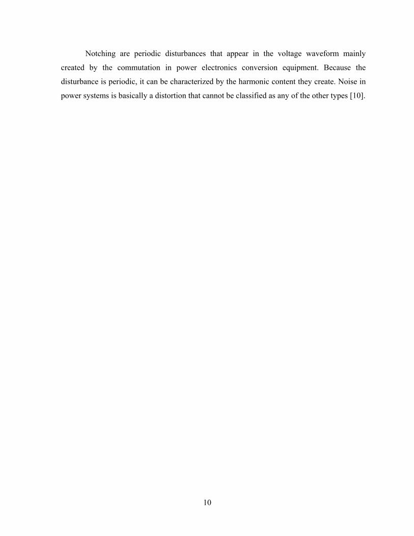
Figure 4.6 represents the diagram of the equivalent circuit of the system: DC loop and
inverter of the SFC, and synchronous machine. The rectifier bridge is represented as the
equivalent voltage source of value Vα connected to the inverter bridge and the synchronous
machine. The inverter is represented as a set of variables sources that controls the currents
and voltages in the d and q circuits.
31
Figure 4.6 Circuit model of the inverter side of the static frequency converter and the
synchronous machine
4.3.2 Parameters of the computer model of the SFC
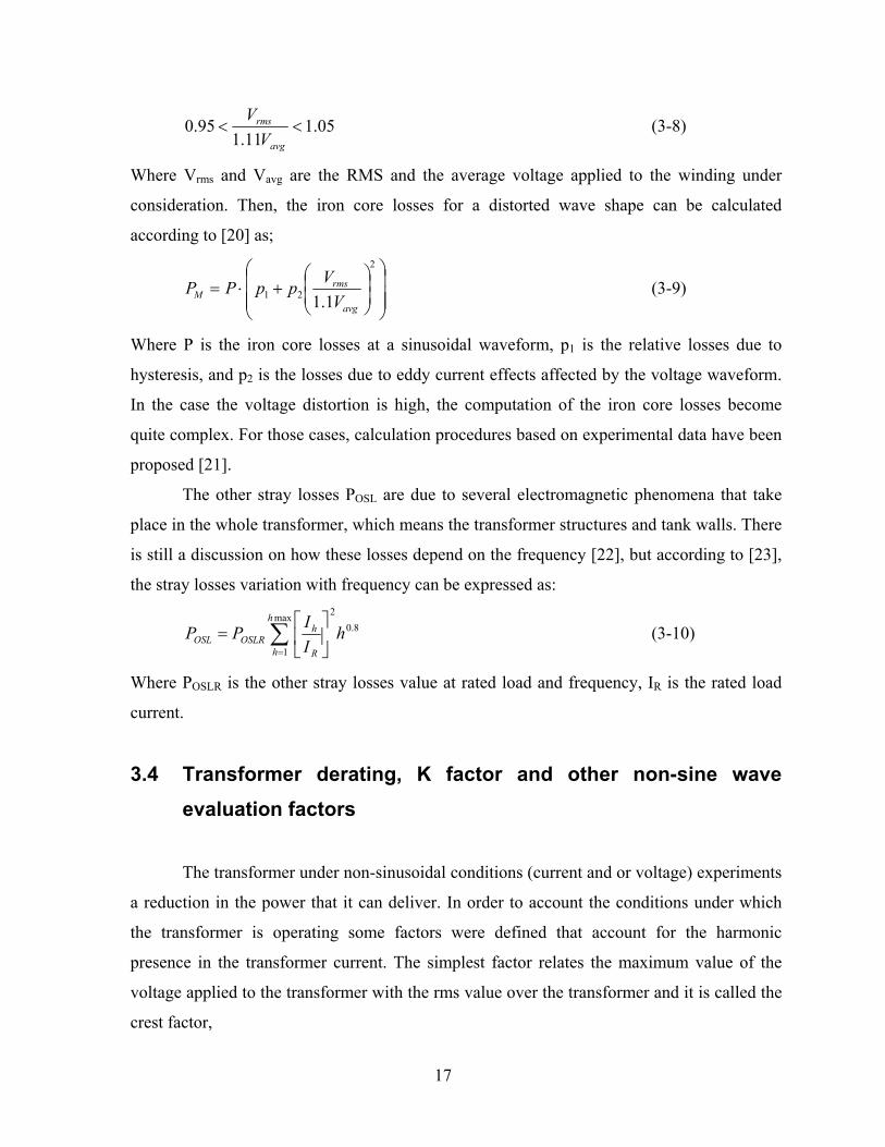
The SFC is composed of a rectifier and a current source inverter linked by two 17 mH
inductors that provide the current source mode. At both the rectifier and inverter side the
converter is fully modeled by a six-pulse thyristor bridge and a GTO inverter bridge
respectively. Each thyristor is modeled as a controlled resistance that changes from a large to
a small value when the conduction process starts (Figure 4.7 and Table 4.3). Snubber circuits
can play a significant roll during the commutation transients; therefore, these circuits are
included in the model, as well as surge arresters at both AC sides of the SFC.
Figure 4.7 Thyristor and snubber circuit
Rs ωr.ΨqsLds -Ldm
Lmd
Rdr Ldr -Ldm
RfdLfd
vfd
iqsiqr
ifd
Lqs -Lqm Rqr Rs ωr.Ψds
Lmq
Lqr -Lqm
iqs iqr
gq ire
gd ire
Tgr1
+
-
LF RF
Vα
gd Vd
gq Vq
ire +
-
+
-

32
Table 4.3 Main parameters for the thyristor model. The snubber circuit parameters were taken
from a previous study
Thyristor On resistance [Ω] 0.01 Thyristor Off resistance [Ω] 1.0e6 Forward voltage drop [V] 1.0 Forward/reverse withstand volt[V] 1.0e5 Snubber resistance [Ω] 9200 Snubber capacitance [uF] 0.002
4.4 GSU Transformer
The generation step up (GSU) transformer plays a major role in this study. This
transformer is not only relevant for the electric disturbance propagation phenomenon, but it
has also suffered some failures in recent times becoming the object of major concern.
Therefore, special carefulness is necessary in the transformer modeling. However, due to the
frequency range under analysis, it is not necessary to study the electromagnetic phenomenon
propagation inside the transformer windings. An appropriate terminal model is accurate
enough for the purpose of this study. A comprehensive description of different transformer
terminal models for computer transient studies can be found in [35], and for harmonic studies
in [36], [37].
The simulations were done using three single-phase transformer models properly
connected. The constructive characteristic of the transformer, with three isolated tanks where
each phase core and windings lie, justifies the single-phase modeling. This modeling does
not introduce an error and greatly simplifies the analysis because no inter-phase mutual
coupling of any type needs to be considered. The PSCAD/EMTDC program provides built-in
subroutines for the simulation of transformer models [38]. However, these subroutines are
built over several assumptions and model considerations that need to be checked.
The transformer models provided in EMTDC—the study employed TSAT21—are 60
Hz models. The TSAT21 supports magnetic saturation, losses and the most relevant
phenomena around the fundamental frequency. Core saturation, which can play an important
role if ferro-resonances are developed, is modeled as a variable current source connected in
parallel with the winding wound closest to the core. The current value is controlled by the

33
voltage over the connected winding and the transformer magnetic characteristic. In addition,
the magnetizing current and no-load losses are represented in a simplified way by the
resistance R0. Although being complete at 60Hz, the model is not appropriate above 3 kHz.
At this frequency the winding distributed capacitances must be considered. This is especially
true when the voltage transfer between windings plays an important role in the analysis, as
can be the case of this study. Therefore, the surge capacitances Cs1, Cs2 and Cs12, which are
not originally provided in the EMTDC routine, are added in the model producing the result of
Figure 4.8.
Figure 4.8 Single-phase transformer model
The transformer test data provide information for calculation of the parameters at 60
Hz. Standard values from the literature were used for the surge capacitances. The values for
the transformer employed in the study are shown in Table 4.4. Although based on all the
previous considerations, the model for simulation in PSCAD requires a different input
format. Table 4.5 shows the main data of the transformer in the format required by the
program.
Table 4.4 Transformer equivalent circuit parameters
Branch L [mH] R[Ω] C[nF]
Primary LV 22 3.82 e-3 0.5
Secondary HV 1030 0.4 5.0
Magnetizing - 6416 -
Inter-winding - - 0.3
L1 L2 R2 R1
Isat
R0
1:a

34
Table 4.5 Transformer configuration data for EMTDC simulation
Main parameters Rated Power [MVA] 100 Short circuit reactance [pu] 0.1645 Magnetizing current [%] 0.066 No-load losses [pu] 4.24e-4 Ideal transformer modeling (#) Yes
Saturation parameters Air core reactance Xair [pu] 27.06 Inrush decay time constant [sec] (*) 0.5 Knee voltage [pu] 1.085 Time to release flux clipping [sec] (°) 0.1 Saturation placed on winding 1 (#) Magnetizing current provided by only the saturation branch. (*) Depends also on the network, realistic value (°) Simulation parameter, for starting simulation purpose
Attention is given in this study to the possible presence of saturation phenomena. The
transformer magnetizing curve provides the data for the saturation calculation. Instead of
using all the data of the magnetizing curve, EMTDC simulates the saturation characteristic
based on the most relevant saturation values. The calculation of these saturation values, taken
from [38], is described as follows. The flux in the magnetic core, ΦR, is calculated by the
expression,
∫=Φ dttvR )(
Considering a sine voltage,
tVtv ωsin)( max=
and replacing values in the flux expression results,
tR ωsin89.61=Φ
The air core reactance is calculated by the ratio of flux ∆ΦM and current ∆IM of two points of
the magnetizing curve while in saturation by the following expression;
bM
MAIR ZI
X ω∆∆Φ
=

35
replacing with the transformer values, the air core reactance and air core inductance are
calculated as,
XAIR = 27.06 pu
LAIR = 195.4 mH
Other important parameter is the knee point (XKNEE) that gives the relation between
the point at which the magnetizing curve intersects the flux ax and the rated flux. This value
is given by the expression,
R
MaxAIRMaxKNEE
ILX
Φ−Φ
=
where ΦMax and IMax correspond to the extreme point of the characteristic and ΦR is the peak
value of the rated flux. Replacing in the formula, the value calculated for XKNEE is,
XKNEE = 1.085
which is inside the standard limits of 1.0 < XKNEE < 1.2. All these calculated values produce
the simplified magnetizing curve shown in Figure 4.9.
Magnetizing curve
0
4
8
12
16
20
24
0 10 20 30 40Current [A]
Volta
ge [k
V]
Figure 4.9 Simplified magnetizing curve

36
4.5 Transmission Cable
A distributed parameters line model with frequency dependent parameters is used for
modeling the 345 kV cable. The election of the model is based on the simulation time step
and the transient phenomena under analysis. The distributed parameter model is widely
described in the literature [3], [38] With the use of the forward and backward propagation
waves (F and B) and the surge impedance (zo) the relation between voltages (V) and currents
(I) at one of the line ends k can be expressed as,
)()()()( ωωωω kokk izVF ⋅+=
)()()()( ωωωω kokk izVB ⋅−=
which are similar for the other end of the line. These equations can be represented in the
equivalent circuit of the line shown in Figure 4.10. The relation between both line ends is
given by the equations:
)()()( ωωω mk FAB ⋅=
)()()( ωωω km FAB ⋅=
Where LeA )()( ωγω −=
is known as the propagation constant composed by the attenuation and phase constant. And L
is the length of the line.
Figure 4.10 Equivalent circuit of the frequency dependent line model
The product in the frequency domain relating the forward and backward waves
implies a convolution in the time domain that is solved in the computer by numerical
+- Bk(ω)
Zo(ω)
ik(ω)
Vk(ω)
+-Bm(ω)
Zo(ω)
im(ω)
Vm(ω)

37
algorithms. For the calculation of that convolution the matrix A(ω) is numerically
approximated by a curve fitting technique. EMTDC calculates the cable parameters based on
the cable constructional characteristics, and the same curve fitting routine for A(ω), to
calculate the surge impedance zo(ω) at different frequencies. The range of frequency where
the cable model is approximated is selected between 1 Hz and 1 MHz, which comprises the
range of 5 Hz-20 kHz of the complete system model. Figure 4.11 shows the surge impedance
as a function of the frequency.
The representation of three-phase transmission systems requires taking into
consideration the different propagation modes that appear when more than one conductor
exists. It is possible to simplify the analysis by decomposing the propagation phenomena in
the different modes as each mode can be treated as a single transmission line. A
transformation matrix relates the modal and circuit voltages and currents. That
transformation is described by the equations:
[ ] [ ] [ ]eeph VTV mod⋅=
[ ] [ ] [ ]eiph ITI mod⋅=
[ ] [ ] 1−= iT
e TT
Where:
[ ] [ ] currentsandvoltagesphaselineIV phph =,
[ ] [ ] currentsandvoltageseIV ee mod, modmod =
[ ] [ ] currentsandvoltagesformatrixtiontransformaTT ie =,
An eigenvalue technique is used for the calculation of the matrices Te and Ti.
Harmonic studies require the use of a three-phase model due to the possibilities of
interaction between phases. Therefore, a complete three-phase model of the whole system
was developed for this study including three-phase representation of all the components.
Nevertheless, in cable modeling the inclusion of the three phases ad more complexity due to
the several propagation modes that appear when a multi-conductor system is considered.
Besides, according to the cable data all the cable sheaths are directly grounded, this fact gives
certain independence to the phenomenon of propagation in each phase. So, under this
condition of electromagnetic isolation, a simplification of the cable model and the use of

38
three parallel single-phase cables is acceptable. The two cable models were implemented for
this project and the closeness of the results totally supports the introduction of the single-
phase simplification.
The value of the surge impedance calculated by EMTDC, Z0 = 38.21 Ω, fully
coincides with the value used in the previous parts of this study. Please refer to Appendix A
for the cable physical data, parameters for calculation and solved constants.
Figure 4.11 Frequency dependence of the cable surge impedance
100 101 102 103 104 105 10630
40
50
60
70
80
90
100
110
120
130S urge Im pedance
frec [Hz ]
Zo [o
hm]
39
5 Control Strategy of the Static Frequency Converter
The representation of the synchronous machine in the dqo coordinates can be used to
calculate the electromagnetic torque in the motor, which is given by the following equation:
( )dsqsqsdse iipT ψψ −=22
3 (5-1)
The meaning of each one of the variable notations appearing in this equation and the next
ones has already been given in chapter three. Following [28], [39], and replacing in this last
expression with the flux equations (4-4), the torque expression becomes,
( ) ( )( )dsqrmqqsqsqsdrmdfdmddsdse iiLiLiiLiLiLpT ′+−′+′+=22
3 (5-2)
Considering only the first order harmonic component of the stator currents, the current ids is
null, then the torque expression can be simplified to:
( ) qsdrfdmde iiiLpT ′+′=22
3 (5-3)
From this expression it is possible to see that the torque can be controlled by regulating the
current iqs. Therefore, controlling the current supplied by the inverter is possible to control
the electric torque in the machine.
The control strategy of the SFC converter used for synchronous machine starting is
divided in two stages as described in [40], [41]. The first one requires forced commutation
until 8-10% (32-40 rpm) of the machine rated speed, 400 rpm. The second stage uses natural
commutation supported by the voltage induced in the machine windings. During the first
stage, the voltage applied to the machine is relatively low; therefore, the voltage magnitude
on the high voltage side of the transformer will be also low. However, if large voltage
distortion is produced during the forced commutation creating large spikes, harmful effects
could appear over the transformer windings. In the second stage, while using natural
commutation, the machine control strategy keeps a constant flux level in the magnetic circuit.
The acceleration process increases the operation frequency. Therefore, the voltage level is
increased in the same proportion, because the relationship
V/f = constant,
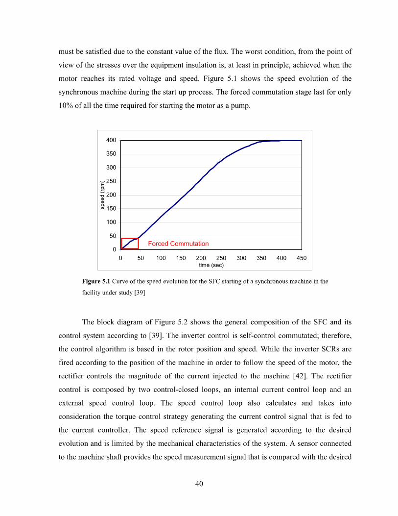
40
must be satisfied due to the constant value of the flux. The worst condition, from the point of
view of the stresses over the equipment insulation is, at least in principle, achieved when the
motor reaches its rated voltage and speed. Figure 5.1 shows the speed evolution of the
synchronous machine during the start up process. The forced commutation stage last for only
10% of all the time required for starting the motor as a pump.
0
50
100
150
200
250
300
350
400
0 50 100 150 200 250 300 350 400 450time (sec)
spee
d (rp
m)
Figure 5.1 Curve of the speed evolution for the SFC starting of a synchronous machine in the
facility under study [39]
The block diagram of Figure 5.2 shows the general composition of the SFC and its
control system according to [39]. The inverter control is self-control commutated; therefore,
the control algorithm is based in the rotor position and speed. While the inverter SCRs are
fired according to the position of the machine in order to follow the speed of the motor, the
rectifier controls the magnitude of the current injected to the machine [42]. The rectifier
control is composed by two control-closed loops, an internal current control loop and an
external speed control loop. The speed control loop also calculates and takes into
consideration the torque control strategy generating the current control signal that is fed to
the current controller. The speed reference signal is generated according to the desired
evolution and is limited by the mechanical characteristics of the system. A sensor connected
to the machine shaft provides the speed measurement signal that is compared with the desired
Forced Commutation

41
value closing the control loop. According to the torque control strategy the corresponding
current value is generated, which is also properly limited according to the system constraints.
Finally, the current control loop produces the firing angle for the thyristors in the rectifier. A
phase locked loop acts over the controllers synchronizing the pulses with the network
voltage. In this way, the rectifier provides the proper value of current according to the desired
speed and torque, and the inverter takes care of feeding the motor with that current at the
right rotor position in order to reach the desired speed evolution.
Figure 5.2 Circuit model of the static frequency converter
5.1 Inverter Control
As it was explained in the previous section, the phase angle for firing the thyristors in
the inverter is based in the self-commutation strategy. This strategy is based in measuring the
time delay the semiconductor is inversely polarized and the control maintains the inverse
polarization time interval at a safe value. If the angle of inverse polarization is kept constant
then the synchronous machine behaves as brush less dc motor. This behavior is very
convenient from the point of view of the dynamic characteristics that the system presents
being also quite simple to control.
The principle of the self-commutation process is described in [28], [42]. A typical
thyristor voltage commutation evolution is shown in the Figure 5.3. The angle µ is measured
Filter InverterRectifier
Machine
Current Controller
Current Limiter
Speed & Torque Control
Inverter Controller
Phase lock loop
Filter InverterRectifier
Machine
Filter InverterRectifier
Machine
Current Controller
Current Limiter
Speed & Torque Control
Inverter Controller
Phase lock loop
Current Controller
Current Limiter
Speed & Torque Control
Inverter Controller
Phase lock loop

42
from the power circuit while γ is generally estimated, then according to the desired firing
angle and rotor position, the firing pulses are produced. The firing angle will control the
angle that the armature reaction will have, relatively to the main field flux. In the case of the
application under analysis the armature reaction value will be relatively low as the current is
considerably smaller than the machine rated current. Therefore, the main flux in the machine
magnetic circuit is maintained constant by keeping constant the field produced by the
excitation winding, which means that the excitation regime is approximately constant during
the starting process.
Figure 5.3 Commutation process of a semiconductor in the SFC inverter
The Figure 5.4 shows the phasor diagram of the machine voltage, current and fluxes.
Where V and I are the line currents at the inverter output; Ψf, Ψa and Ψs are the main,
armature reaction, and air gap fluxes, respectively. The angle between the main field flux and
the armature reaction φ’ is the thyristor firing angle because Ψs is directly related with the
rotor angle; and Ψa is created by the armature currents produced by the inverter. From the
figure, it is possible to establish the relation,
αφ −= o180'
As α can be calculated as,
φα −−= vo90
It is valid that,
φφ ++= ov 90'
γ
µ
β

43
The power factor angle φ between V and I can be approximated as,
µγβφ +=≅
where γ and µ are the indicated in Figure 5.3. Then the thyristor firing angle can be
calculated as,
µγφ +++= ov 90'
For the calculation of φ’, regular practices take measurement of the angle µ while estimate v
and γ [28].
Figure 5.5 shows the block diagram of the rectifier control circuit as it was
implemented for this study. The angle µ was measured by the configuration proposed in [43]
and proper values for v and γ where estimated after some simulations.
Figure 5.4 Phasor diagram of the synchronous machine voltages and fluxes
Filter InverterRectifier
filter
φ’Firing pulses
Machine
Pulse processor
angle
R Q
S
OR
ORπ/2+γ+v
µ
γmeasured
Filter InverterRectifier
filter
φ’Firing pulses
Machine
Pulse processor
angle
R Q
S
R Q
S
OROR
ORORπ/2+γ+v
µ
γmeasured
Figure 5.5 Block diagram of the inverter control circuit
φφ
90°α
φ’v
V
I
ΨaΨs
Ψf

44
5.2 Rectifier Control
The rectifier provides the necessary current in the DC interface of the SFC. That
desired value of current is computed by the rectifier control loop that is composed by two
control loops. The inner loop is the current controller, which is basically a controller that
calculates the thyristor firing angle according to the reference and actual value of current.
The outer control loop is the speed controller that generates the current reference value from
the desired speed evolution and according to the torque control strategy. This configuration
of the controller is widely used in different applications of machine control [44]. In the
application considered in this study, it is usually desired to have a constant torque control
during the self-commutated stage, from 10% to 100% of the rated speed. In this way the
acceleration is kept constant and the speed increases uniformly. The torque control is
maintained constant by keeping the DC current constant and therefore the corresponding AC
current in the machine phases constant. According to equation (3-3) the torque depends on
the stator current value and the field current. Because the field flux is desired to be constant,
and the armature reaction can be considered very low, the flux is approximately constant if
the field current is constant. Figure 5.6 shows the block diagram of the rectifier control as it
was implemented for this study.
Figure 5.6 Block diagram of the control system of the SFC rectifier
Filter InverterRectifier
cos-1
Phase Lock Loop
Pulse processor
α
Current Controller
ω Ire
ωr
Speed Controller
Limiter
Filter InverterRectifier
cos-1
Phase Lock Loop
Pulse processor
α
Current Controller
ω Ire
ωr
Speed Controller
Limiter

45
In Figure 5.6 ω and ωr represent the measured and reference current value respectively;
Ire is the DC measured current and α the firing angle computed by the controller. The pulse
processor generates the pulses for the thyristor firing with the signal received from the
controller and synchronize them with the line voltages by making use of a phase locked loop.
The controllers provided in each one of the loops are of the proportional integral (PI) type.
5.3 Forced Commutation Stage
During the first stage of the starting process, the voltage generated by the synchronous
machine is not enough to force the commutation of the thyristors in the inverter [1].
Therefore, a mechanism to force the commutation must be developed in order to transfer the
current form one of the branches of the inverter bridge to another. In the SFC, the
commutation mechanism simply consists of changing the branch under conduction while the
DC current has been reduced to zero. The DC current cancellation is achieved by changing
the operation mode of the bridge from rectifier to inverter. In a thyristor bridge, the direction
of the power flow is related with the firing angle; the relation between the firing angle and
the voltage at both sides of the bridge is given by,
fLLdc VV απ
cos3=
Where Vdc is the voltage in the DC side, VLL is the line-line voltage in the AC side, and αf is
the firing angle. If the firing angle is greater than 90 degrees the bridge load flow is from the
DC side to the AC side acting as an inverter. The firing angle is then changed in order to
revert the voltage on the DC interface and cancel the DC current [45].
When the current is zero, the SCR in the previously conducting branch of the inverter
is turned off, then a new SCR in another branch is fired and the rectifier is re-started. The
operation of this commutation mechanism is allowed by the large difference between the
operating frequencies of both parts of the converter. Figure 5.7 shows the firing sequence of
the inverter bridge, and the theoretic waveforms of the currents in the SFC output while in
the forced commutation stage. In the middle of each conduction period the current is

46
interrupted by a time interval long enough to assure that the previously conducting thyristor
in the inverter will not be re-ignited when the rectifier is re-started.
Figure 5.7 Three-phase current waveforms and forced commutation sequence in the inverter
bridge
6-1 1-2 2-3
1 1
4
4-53-4 5-6 5-6
1
4
3 3
6 6
5 5
2 2

47
6 Operation Conditions
The main purpose of the study is to analyze the effects of the SFC operation over the
HV equipment. The SFC is employed during the start up process of the synchronous machine
in the pump mode. At this stage, although it is not operatively necessary, the high voltage
transformer remains connected to the SFC and the starting machine. A simplified schematic
of the system configuration during the SFC operation is shown in Figure 6.1. And a complete
diagram of the system under analysis can be observed in Appendix A. The voltage seen at the
low voltage side of the transformer, as well as its distortion content, is then transferred to the
high voltage side, which is connected to the high voltage transmission cable. The goal at this
point is to determine the electric stresses over the subsystem composed by the SFC,
synchronous machine, transformer, and high voltage cable. This subsystem operates on a
wide range of frequencies and voltage levels. Therefore, it is important to determine the
operation conditions that produce the largest stresses over the equipment.
Synchronous machine
Static frequency converter
GSU Transformer
Cable
Synchronous machine
Static frequency converter
GSU Transformer
Cable
Figure 6.1 Schematic of the SFC starting system
As it was explained in section chapter five the rated voltage is applied to the machine
when running at rated speed. Before that operation condition the fundamental voltage is

48
smaller. Therefore, for same operating mode of the SFC it is expected that other operation
conditions at lower speed/ lower voltage will create less harm over the equipment. The first
step was then to simulate the system operation at its rated values –that is, with the SFC
supplying rated voltage and frequency. This rated parameters are shown in Table 6.1 It was
also check that other operation conditions at reduced speed or reduced load do not create
harmful voltages or currents on the GSU transformer.
During the forced commutation stage, the operation of the SFC is different than the
natural commutation operation as it was described in 5.3. Therefore, in spite the voltage at
the forced commutation mode is too low due to the very slow speed, it is necessary to check
the proper operation of the SFC at that stage and the absence of dangerous conditions on the
HV equipment. On the contingency operation aspect it is worth noting that there are not too
many possible contingencies due to the simplicity of the starting system\ as seen in Figure
6.1. The simulation of some contingencies can like HV cable disconnection or loss of neutral
connection can help to understand the role of the different system components on the
behavior of the whole system.
Table 6.1 SFC parameters at the rated operating condition
Voltage [KV] 16500
SFC current [A] 1050
Power at motor [MW] 12
Field speed [rad/sec] 377

49
7 Harmonic Analysis of the System
There are different methods to analyze the harmonic propagation in an electric
network; a compendium of them can be found in [9]. The methods for harmonic analysis can
be generally classified in frequency domain and time domain methods. Frequency domain
methods include frequency scan, harmonic penetration and harmonic load flow. On the other
side, the time domain analysis methods are based in the calculation of the time evolution of
the system magnitudes that generally is done by simulation of the operation. This chapter is
dedicated to the frequency domain analysis while the next one to the time domain analysis of
the system under study.
7.1 Frequency Domain Methodologies for Harmonic Analysis
Frequency domain methodologies base the analysis in the matrix admittance
representation of the network under study. That representation of the network can be single
or multi phase based according to the type of study and the degree of precision required. For
a generic network like the one in figure 7.1, the admittance matrix is obtained from the
models of each of the components in the network and is,
=
NNNNN
N
N
N V
VV
yyy
yyyyyy
I
II
M
L
MM
L
M2
1
21
22221
11211
2
1
(7-1)
Where Ij, j=1,…N are the mutual currents in the network nodes, V j, j=1,…N are the voltage at the
network nodes, yjj is the proper admittance of the matrix nodes, and yij, i≠j is the mutual
impedance between two network nodes. The yij coefficients are generically calculated from;
ikNkkIVI
yj
iij
≠===
,1,0 L

50
Figure 7.1 Generic electrical network
A frequency scan provides the response of the system to electric voltage or current at
different frequencies. Because of its simplicity and usefulness, a frequency scan is usually
the first step of every harmonic study and is also very suitable for transient studies [9]. The
scan provides a first picture of the system behavior for a wide frequency range, allowing
detection of possible problems that otherwise would be difficult to cover with time domain
simulations at different system conditions. The scan study is done from one of the points in
the network called the driving point. From this point a variable frequency current (or voltage)
is injected into the network, the voltage (or current) response is measured at the same point
or another point of interest and the result is usually given as a frequency-impedance plot. The
range of variation of the source frequency depends on the type of study being developed. The
injected current will generate a set of network voltages according to the admittance equation
[ ] )(~)()(~ hVhYhI = (7-2)
Where Y(h) is a network admittance matrix, whose parameters must be valid over the whole
range of study; Ĩ the array of network currents when one current is injected and V the set of
voltages generated by the current injection. For a unitary current, the voltage value coincides
with the impedance seen from the driving point.
It is also possible to do a frequency scan by feeding the network with a voltage source
and calculating (or measuring) all the other voltage values in the network. In this case the
relation obtained is called the voltage transfer function. The election of feeding the system
with a voltage or a current source depends on the purpose of the frequency scan study. For
V1
V2
VN
NetworkI1
IN
I2
~
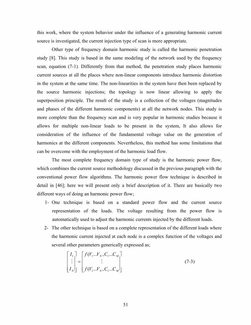
51
this work, where the system behavior under the influence of a generating harmonic current
source is investigated, the current injection type of scan is more appropriate.
Other type of frequency domain harmonic study is called the harmonic penetration
study [8]. This study is based in the same modeling of the network used by the frequency
scan, equation (7-1). Differently from that method, the penetration study places harmonic
current sources at all the places where non-linear components introduce harmonic distortion
in the system at the same time. The non-linearities in the system have then been replaced by
the source harmonic injections; the topology is now linear allowing to apply the
superposition principle. The result of the study is a collection of the voltages (magnitudes
and phases of the different harmonic components) at all the network nodes. This study is
more complete than the frequency scan and is very popular in harmonic studies because it
allows for multiple non-linear loads to be present in the system, It also allows for
consideration of the influence of the fundamental voltage value on the generation of
harmonics at the different components. Nevertheless, this method has some limitations that
can be overcome with the employment of the harmonic load flow.
The most complete frequency domain type of study is the harmonic power flow,
which combines the current source methodology discussed in the previous paragraph with the
conventional power flow algorithms. The harmonic power flow technique is described in
detail in [46]; here we will present only a brief description of it. There are basically two
different ways of doing an harmonic power flow;
1- One technique is based on a standard power flow and the current source
representation of the loads. The voltage resulting from the power flow is
automatically used to adjust the harmonic currents injected by the different loads.
2- The other technique is based on a complete representation of the different loads where
the harmonic current injected at each node is a complex function of the voltages and
several other parameters generically expressed as;
=
MN
MN
N CCVVf
CCVVf
I
I
...,...(
...,...(
11
111
MM (7-3)

52
where the parameters Ci represent the dependence of the load with parameters such as
the motor speed –in case of a drive, etc. This technique is much more complex and
complete and give the most accurate results.
In this study a combination of both frequency and time domain analysis were employed. The
frequency scan was used to seek for preliminary results and provide some orientation for the
study. Otherwise, the time domain simulation was widely used to study not only the effects
of the harmonic components existing in the system but also other phenomena such as the
magnitude of commutation transients and notches generated by the SFC operation.
7.2 Frequency Scan of the System Components
As previously stated the subsystem SFC, generator, transformer, and cable is an
object of major attention. Therefore, several frequency scans were carried out to get the
frequency behavior at these critical circuit elements. EMTDC provides an easy way to
perform frequency scan with a variable frequency current source that can be placed in the
driving point of interest. Because the goal was to obtain the frequency response over a wide
range covering the harmonic and transient spectrum, we made the scan in two ranges for a
better visualization. One range covers up to 200 kHz and the other only up to 5 kHz. Figure
7.3.1 shows the circuit disposition for the scan of the transmission cable.
Vcaba VcababVtlab
Vtlbc
0.001
0.001
0.001
Iatl
Ibtl
Ictl
Vtlca
Va
Vb
Vc
C1cablemin C1cablemin
cablemin
C1cablemin2
cablemin2
C1cablemin3 C1cablemin3
cablemin3
C1cablemin2
A
B
C
Harm.CurrentInjection
Figure 7.2 Circuit for cable frequency scan showing the variable frequency source, cable and
different meters
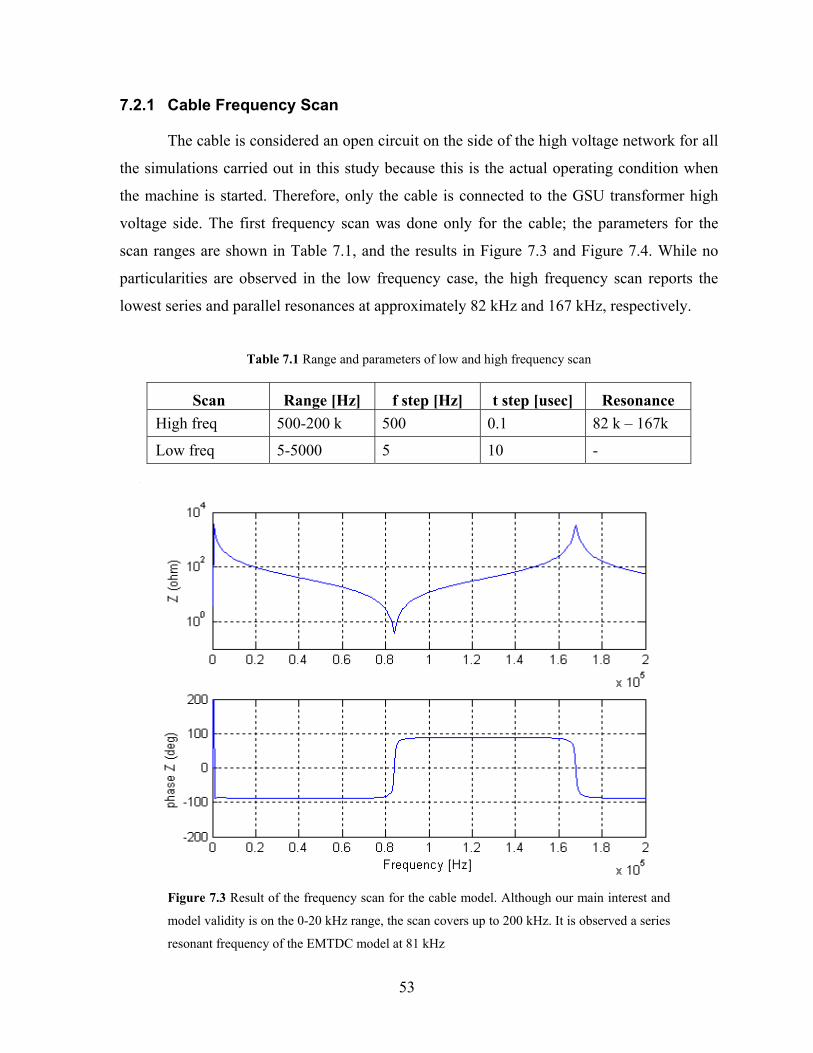
53
7.2.1 Cable Frequency Scan
The cable is considered an open circuit on the side of the high voltage network for all
the simulations carried out in this study because this is the actual operating condition when
the machine is started. Therefore, only the cable is connected to the GSU transformer high
voltage side. The first frequency scan was done only for the cable; the parameters for the
scan ranges are shown in Table 7.1, and the results in Figure 7.3 and Figure 7.4. While no
particularities are observed in the low frequency case, the high frequency scan reports the
lowest series and parallel resonances at approximately 82 kHz and 167 kHz, respectively.
Table 7.1 Range and parameters of low and high frequency scan
Scan Range [Hz] f step [Hz] t step [usec] Resonance High freq 500-200 k 500 0.1 82 k – 167k
Low freq 5-5000 5 10 -
Figure 7.3 Result of the frequency scan for the cable model. Although our main interest and
model validity is on the 0-20 kHz range, the scan covers up to 200 kHz. It is observed a series
resonant frequency of the EMTDC model at 81 kHz

54
Figure 7.4 Result of the frequency scan for the cable model on the low frequency range
7.2.2 Cable and Transformer Frequency Scan
The next step of the study was to determine the frequency response of the cable and
the GSU transformer. This characteristic is useful to understand the response to surges
reaching the transformer. Therefore, a frequency scan with a driving point for z(ω) at the low
voltage side of the GSU was performed. The scan was done on both frequency ranges of
Table 2.1. Because of the transformer, the response at low frequencies is primarily inductive.
When frequency increases, the surge capacitances appear, and after a resonance at around
195 kHz, the capacitance effect dominates the frequency response. Note that because 195
kHz is above the frequency range where this model is valid, this resonant frequency can have
certain degree of uncertainty. Figure 7.5 shows the high-range scan characteristic; the low
frequency plot does not present any interest and is omitted. The response at the internal nodes
is not considered at this stage of the analysis. The circuit diagram is similar to the complete
set cable, transformer and generator scan (without the generator branch) that is shown in
Figure 7.6.
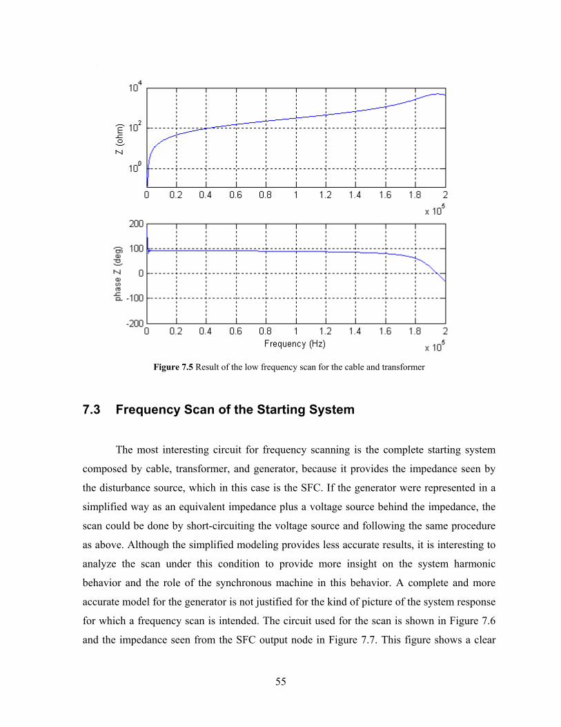
55
Figure 7.5 Result of the low frequency scan for the cable and transformer
7.3 Frequency Scan of the Starting System
The most interesting circuit for frequency scanning is the complete starting system
composed by cable, transformer, and generator, because it provides the impedance seen by
the disturbance source, which in this case is the SFC. If the generator were represented in a
simplified way as an equivalent impedance plus a voltage source behind the impedance, the
scan could be done by short-circuiting the voltage source and following the same procedure
as above. Although the simplified modeling provides less accurate results, it is interesting to
analyze the scan under this condition to provide more insight on the system harmonic
behavior and the role of the synchronous machine in this behavior. A complete and more
accurate model for the generator is not justified for the kind of picture of the system response
for which a frequency scan is intended. The circuit used for the scan is shown in Figure 7.6
and the impedance seen from the SFC output node in Figure 7.7. This figure shows a clear

56
parallel resonance around 820Hz (13th harmonic) and some other resonant frequencies
around 1250Hz (21st harmonic).
Vtlbc
0.001
0.001
Va
C1cablemin C1cablemin
C1cablemin2
C1cablemin3
0.001
C1cablemin3
cablemin3
C1cablemin2
cablemin2
0.001
0.001
0.001
0.02
0.02
0.02
1310.0
cablemin
Vas Vtlab
Ias
0.0003
0.0003
0.0003
#1 #2
#1 #2
0.0005
0.00
5
0.00050.0005
0.00
50.
005
#1 #2
Iatl
0.00
053
0.00
053
0.00
053
A
B
C
Harm.CurrentInjection
Figure 7.6 Frequency scan circuit for the cable, transformer and generator group
Figure 7.7 Frequency response of the cable, generator and transformer group

57
7.4 Analysis of Frequency Scan Results
Several resonances are observed in the impedance characteristics obtained from the
frequency scans. The cable presents a resonant frequency at 82 kHz which is consistent with
other studies done over this same cable [16]. The scan with the simplified model of the
generator shows resonant frequencies at some frequency values that can possibly amplify
harmonic components existing in the circuit. Because of some differences that exist between
the simplified model and the actual generator, it is necessary to investigate how much of
these possible resonances appear in the real case. The time domain simulation in the
following chapter provides more insight on this subject.
The frequency scan at several driving points was done to get a first picture of the
system response at different frequencies. A time domain simulation based on the operating
conditions described in chapter six followed the scan study. Based on this basic information,
some other cases were simulated in order to get a better understanding of how the system
behaves. Finally, the results are analyzed on both different aspects: harmonics and transients
generated by the thyristor commutation.

58
8 Time Domain Simulation
Time domain methods for the analysis of electric systems are generally more accurate
than other frequency domain techniques such as power flow; on the other side, they are more
complex to implement [46]. Some special conditions existing in the power system cannot be
represented accurately by the power flow technique requiring the use of time domain
simulation. These conditions can be summarized as:
1- The distortion produced by the devices can vary according to the conditions under
which they are working. And this fact cannot be properly described by an equation
like (7-3).
2- Interactions between different harmonic orders cannot be represented by time
invariant models as the ones used for harmonic power flow.
3- When power electronic conversion is used, the presence of distortion in the system
magnitudes can influence on the control of the gating signals.
Moreover, the time domain simulation allows the simultaneous existence of all the electric
phenomena existing in the actual system operation like the transients produced by the
switching of the power electronic devices that compose the energy converters.
In addition to a proper modeling of the different systems components, as developed in
chapter four, some other consideration should be made in order to obtain accurate results
from a time domain simulation of the system behavior. These considerations include the
proper calculation of the initialization process and magnitude of the different variables.
Some physical phenomena as the magnetic flux in electrical machines may take a relatively
long time to reach its steady state regime. The loops associated to the control schemes of the
power electronic converters can require special initialization procedures. The extinction of
the transient phenomena related to the initialization process must be verified before using the
data for the analysis.
In this work the harmonic phenomena and the commutation transient are, at least
preliminarily, studied from the same models according to the modeling considerations
previously explained. The simulation parameters (time step, etc.) are different according to
the type of investigation. The complete system was modeled in EMTDC/PSCAD according

59
to the guidelines and conditions described in chapter four and the complete circuit diagram is
shown in Appendix A. The base case is the SFC operating at its rated conditions. In addition,
some other conditions were studied and the waveforms obtained for those cases are included
when considered useful for the analysis.
8.1 Rated Operating Conditions (Base case)
The analysis of the electric magnitudes and their harmonic content at different points
of the system allow analyzing the stress levels and effects over the equipment. In addition,
with the analysis it is possible to infer the action each component has in the behavior of the
complete system and its electrical magnitudes. The data in this section is presented in a way
intended to help the analysis. First the voltages at different nodes are analyzed and then the
currents and some other magnitudes if relevant. The waveforms are presented in a sequence
starting at the far end of the cable and going through the different components until the
supplying voltage source at the MV auxiliary bus of the station. Each waveform plot shows a
two-cycle waveform plus the harmonic spectrum of that waveform. On the harmonic charts,
the relative content is related to the fundamental component, which implies that the
fundamental percentage is always one hundred. The names of the signals refer to the names
in the circuit diagram in Appendix A. In this chapter only a reduced set of waveforms are
included for each simulation case. A complete set of waveforms for the different tested cases
can be seen at the Appendix B.
Figure 4.1 shows the voltage at the transformer HV side. It is observed the important
level of 13th harmonic and a relatively high total harmonic distortion. The harmonic content
does not considerably increase the maximum voltage value; a crest factor of 1.64 implies
only a 15% of increment over the maximum voltage under sine wave conditions. The
waveforms of the voltage at both sides of the transformer and at the cable end are completely
similar; therefore, only one is presented here. Table 8.1 shows a comparison between the
harmonic content in the voltage waveforms before and after the transformer. It is possible to
see a reduction in the harmonic content at the transformer low voltage side. This fact
suggests the idea that the cable plays an important role in generating the harmonic generation
and the abnormal level of 13th harmonic.

60
Figure 8.1 Vtab Line –line voltage at the transformer HV terminal. As the cable is not loaded
it is very close to the voltage at the cable open-end
Table 8.1 Harmonic characterization of the voltage at the cable end, and at the GSU low and
high voltage side
Network point THD [%] 13th [%] CF [%]
V cable 12.2 11.0 1.64
V transf HV 12.2 11.0 1.64
V transf LV 8.2 6.9 1.51
The voltage waveforms before and after the SFC are shown in Figure 8.2 and 8.3
respectively. The voltage at the output shows a disproportionate amount of the 13th and 11th
harmonics, which do not follow the general exponential decaying tendency of a phase-
controlled converter [47].

61
Figure 8.2 Vab Line – line voltage at the SFC converter output side, 16.5 kV
Figure 8.3 Vsab Line –line voltage at the converter input side, 16.5kV

62
The major difference between the Figure 8.2 and 8.3 is in the content of the 11th and
13th harmonics. These harmonic orders are generated by the interaction among the equipment
connected at the SFC output, as it is suggested by the resonant frequencies found in the
frequency scan. It is important to note that he presence of harmonic in the SFC input side is
very important being larger than at the output. Therefore, it is possible they create problems
to other equipment connected on the SFC input side. Figure 8.4 shows the line to ground
voltage at the primary side of the SFC auxiliary transformer. Although the harmonic
distortion has been considerable reduced, the level of disturbance is still large and can create
problems in auxiliary equipment and illumination devices. In the facility object of the study
problem created by harmonics over auxiliary equipment has been observed, producing
failures in discharge lamps used for lighting.
Figure 8.4 Vna Line –ground voltage at the auxiliary bus if the station, 13.8 kV.
In the following figures, the current waveforms for the base case are presented. The
sequence of the figures in this case starts at the transformer LV side. Figure 8.5 shows the
current at the primary winding of the GSU transformer. It is possible to see that the harmonic
distortion is very large and the content of the 13th component is even larger than the

63
fundamental. The magnitude of the 13th order current is large considering that the
transformer is unloaded. Figure 8.6 shows the current on the synchronous machine where the
harmonic content is superposed to the stepped current waveform being the 5th and 13th
harmonics the predominant orders.
Making a comparison of the 13th harmonic component at the transformer and
synchronous machine, the content of that harmonic result:
I13= 135 A at the transformer LV line current
I13= 143 A at the synchronous machine input
which are very close values. This fact shows that the 13th harmonic component circulates in
the path between the synchronous machine, GSU transformer and cable; and that the SFC
introduces only a small portion. The waveform of the transformer line current at the LV side
can be observed in Appendix B and is very similar to the one presented in Figure 8.5 with the
expected difference in the third order components due to cancellation by the line-line
addition effect. Figure 8.7 shows the line current at the SFC output with the typical
waveform and harmonic content of a current source inverter.
Figure 8.5 Iatr Phase current at the LV winding of the main transformer, in the delta winding

64
Figure 8.6 Iag Synchronous machine input current
Figure 8.7 Iato SFC output current. There is no major difference with Isa2, the input current
of the SFC

65
The addition of the currents in the delta-wye windings of the auxiliary transformer
makes the current in the primary side of the transformer to have the waveform shown in
Figure 8.8. The harmonic content has no significant change, but the difference in the phase
angle of the components produces a different waveform.
Figure 8.8 Isa SFC input current at the primary side of the auxiliary transformer, 13.8kV
Summarizing the analysis of the voltage and current waveforms for the rated
operation conditions it is possible to reach the following conclusions. The voltage waveform
and harmonic content are according to what can be expected for the type of phase-controlled
rectifier and converter in use, except for the level of the thirteenth harmonic [47]. The
magnitude of that harmonic is considerably larger than what can be expected, especially in
the transformer HV side and the cable terminals. This fact indicates the HV cable as the
amplifier of that harmonic order. Nevertheless, the effect is produced by interactions between
all the system components. The current also presents a considerable amount of thirteenth
harmonic in the GSU transformer and generator. The abnormal levels of that harmonic
component in the voltages and currents are not seen at the SFC input side and the auxiliary

66
bus at 13.8 kV, but the total harmonic content at this points is considerably large and can
have harmful consequences over the equipment connected a that level.
8.2 Other Operating Conditions at Natural Commutation
8.2.1 Effect of the load current on the circuit behavior
The system was also simulated with the machine taking less power from the SFC.
Mechanical and electrical no-load losses define the minimum power the machine takes when
rotating at rated speed and no mechanic load is connected to the shaft. Even though the value
of these losses can be closely approximated and the respective current used for the
simulations, it is important for the harmonic study to see how much of the harmonic
generation changes with the current level. A simulation was carried out at approximately half
of the rated power in order to observe the effect of the current value on the harmonics. This
value of current is closer to the existing in the circuit when the machine is started following
the acceleration characteristic previously presented. A reduced set of charts is included here
for the purpose of comparison, especially when differences appear respect to the base case.
More waveforms can be seen in Appendix B.
Figure 8.9 shows the voltage waveform at the GSU transformer terminals. From there
it is possible to observe a reduction in the total harmonic distortion level. On the other side
the spectra follows a similar pattern to the full load condition with a remarkable
predominance of the 13th order harmonic. In Figure 8.10 it is possible to observe the
waveform of the line-to-line voltage at the output of the SFC. The time-length of the notches
in the waveform has been considerably reduced, as the time of current commutation between
two inverter branches is smaller. This is fact is directly related with the current value. The
total harmonic distortion is also smaller than the full current load case while the harmonic
pattern is the same. The last figure corresponding to this simulation case is Figure 8.11,
which shows the line current at the transformer primary side. From the analysis of the circuit
magnitudes under the condition of reduced load current, it is possible to conclude that a
reduction in the current lowers the harmonic perturbation in all the system. The

67
characteristics of the harmonic and transient phenomena are similar independently of the
current regime, but the level of the harmonic distortion is reduced with the current value.
Figure 8.9 Vtab, line –line voltage at the transformer HV terminal. The harmonic content is
reduced respect to the base case
Figure 8.10 Vab, line – line voltage at the SFC output (the machine side)

68
Figure 8.11 Iat, line current at the LV side of the main transformer
8.2.2 Effect of the system speed on the circuit magnitudes
The system was simulated at a reduced speed while still at natural commutation. At
this point of the starting process, the counter electromagnet motive force c.e.m.f. generated
by the synchronous motor is reduced according to the rule,
ψ⋅∝ fV
Where V is the voltage at the machine terminals, f is the frequency and ψ is the airgap flux.
Because the control strategy is to keep the magnetic flux constant (section 5.1) the voltage is
proportional to the machine frequency and hence the rotor speed.
Figure 8.12 shows the voltage evolution in the HV side of the GSU transformer, in
this case the maximum magnitude is reduced to almost half of the rated voltage while the
harmonic orders present in the spectra vary according to the value of the fundamental
frequency. In the frequency scan, the resonant frequency was found at approximately 820 Hz.
If the fundamental frequency is 30Hz, the related harmonic is,
33.2730
820==n

69
The 27th harmonic is a triplen order harmonic and therefore is canceled on the line
magnitudes. The following closest harmonics is the 29th, which has a considerable value as is
observed in the spectra; also the 25th harmonic is considerable increased. It is possible to
observe how the effect of the parallel resonance shifts the harmonic spectra according to the
system frequency.
Figure 8.12 Vtab Line to line voltage at the high voltage side of the GSU transformer
Figure 8.13 shows the line-to-line voltage at the output of the SFC, which has a shape
close to the rated speed case, but with different harmonic spectra. It is observed an abnormal
reduction in the 29th harmonic in this case; this fact can be originated by a canceling effect
generated by the voltage drop produced by the 29th harmonic current circulating between the
generator and the transformer. The change in the spectra is also valid for the transformer LV
winding current as it is shown in Figure 8.14 being the largest component at half of the rated
speed the 29th harmonic order. The harmonic distortion is increased respect to the base case
due to a reduced value of the fundamental component because the system voltage is reduced.
On the other side, because the voltage harmonic components are not reduced in the same
proportion, a large harmonic flux value exists in the GSU transformer. This harmonic flux

70
will originate large harmonic magnetizing currents at those orders that are observed in Figure
8.14.
Figure 8.13 Vtab Line to line voltage at the high voltage side of the GSU transformer
Figure 8.14 Iatr Current at the transformer LV winding

71
The SFC input and output currents are shown in Figure 8.19. Each of the currents has
the frequency of the system connected to each side of the SFC, which are 60 Hz and 30 Hz.
The harmonic spectra and total distortion is similar at both sides of the converter. Moreover,
the presence of components induced by the circuit resonance at the SFC is small as was
previously discussed in section 8.1.
Figure 8.15 SFC currents (a) at the SFC input the frequency is 60Hz (b) at the SFC output,
f=30Hz
8.2.3 Effect of the transmission cable on the circuit behavior
Other interesting condition for the analysis of the system behavior and the interaction
between the different components is obtained by disconnecting the cable form the HV side of
the GSU transformer. Although this condition is not possible from the point of view of the
operation, it helps to understand the behavior of the equipment under normal operating
conditions. Figure 8.16 shows the voltage waveform at the HV side of the GSU transformer
and its harmonic content. Comparing this result with the previous waveforms at the same
point, it is possible to note a completely different harmonic spectrum. In Figure 8.17 the
current at the LV winding of the GSU transformer shows an important presence of higher

72
order harmonics superposed to the magnetizing current. In Figure 8.18 it can be observed that
the thirteenth harmonic component has almost completely disappeared in the current at the
synchronous machine. This current is almost the same as the current in the SFC output as the
magnetizing current in the transformer is small.
Figure 8.16 Vtab Line –line voltage at the transformer HV terminal
From the analysis of this operation condition, with no cable connected, it is possible
to observe that the abnormal increment in the thirteenth harmonic disappears. On the other
side, higher harmonic orders around the sixtieth component exist in the system but its value
is small. These high order harmonics are also present when the cable is connected but its
presence is hidden by the relatively large value of the harmonic distortion existing in the
system. The magnitude and level of this distortion at relatively high harmonic level is related
with the values of the surges capacitances of the transformer. Because the capacitance values
were estimated during the transformer modeling, some differences with the actual values are
possible, but in any case its relevance is very small.

73
Figure 8.17 Iatr Current at the LV winding of the main transformer, inside the triangle
connection
Figure 8.18 Iag current taken by the synchronous machine
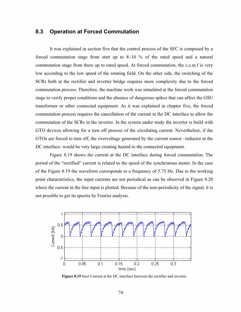
74
8.3 Operation at Forced Commutation
It was explained in section five that the control process of the SFC is composed by a
forced commutation stage from start up to 8~10 % of the rated speed and a natural
commutation stage from there up to rated speed. At forced commutation, the c.e.m.f is very
low according to the low speed of the rotating field. On the other side, the switching of the
SCRs both at the rectifier and inverter bridge requires more complexity due to the forced
commutation process. Therefore, the machine work was simulated at the forced commutation
stage to verify proper conditions and the absence of dangerous spikes that can affect the GSU
transformer or other connected equipment. As it was explained in chapter five, the forced
commutation process requires the cancellation of the current in the DC interface to allow the
commutation of the SCRs in the inverter. In the system under study the inverter is build with
GTO devices allowing for a turn off process of the circulating current. Nevertheless, if the
GTOs are forced to turn off, the overvoltage generated by the current source –inductor at the
DC interface- would be very large creating hazard to the connected equipment.
Figure 8.19 shows the current at the DC interface during forced commutation. The
period of the “rectified” current is related to the speed of the synchronous motor. In the case
of the Figure 8.19 the waveform corresponds to a frequency of 5.75 Hz. Due to the working
point characteristics, the input currents are not periodical as can be observed in Figure 8.20
where the current in the line input is plotted. Because of the non-periodicity of the signal, it is
not possible to get its spectra by Fourier analysis.
Figure 8.19 Irect Current at the DC interface between the rectifier and inverter

75
Figure 8.20 Isa2 Line current at AC three phase input of the SFC, at 16.5 KV
The voltage applied to a SCR in the inverter bridge is shown in Figure 8.21, the
negative spikes correspond to the instant when the current is reduced to zero. At this instant
the rectifier operation mode is switched to inverter mode, then the voltage applied to the DC
loop is inverted and used to cancel the current. As it was also explained in chapter five, the
instant when the voltage at the GTO is negative is used as a control parameter for the
generation of the firing pulses.
Figure 8.21 Et3 Voltage at terminals of a GTO in the inverter bridge
The main purpose of this study was to analyze the electric disturbances at the HV
equipment. Figure 8.22 shows the voltage at the high voltage side of the GSU transformer.
As it is possible to observe in the figure, the magnitude of the voltage is relatively low.

76
Moreover, the relative magnitude of the spikes has been reduced compared to the SFC output
voltage due to some filtering introduced by circuit elements as reactors. The presented
waveforms were obtained with the inverter operating at a frequency approximately of 5.75
Hz. Therefore, the Fourier analysis was done relative to this frequency to get some insight on
the sources generating the higher frequency components. From the spectrum decomposition
it can be observed that a set of components is around the 60th harmonic that corresponds to:
f = 5.75 x 60 = 345 Hz
This frequency is close to the switching frequency of the rectifier of 360 Hz. The other
important set of components is located around the 140th component that corresponds to:
f = 5.75 x 140 = 805 Hz
which is close to the parallel resonant frequency of the circuit detected at 820 Hz.
Figure 8.22 Vtab Line to line voltage at the GSU transformer HV winding
The current at he LV winding of the transformer is shown in Figure 8.23. The current
spectrum has large components around 820 Hz and 345 Hz similar to the voltage spectrum.
The components around 820 Hz are related with the natural resonance of the circuit and is
present during all the starting process. The components around 345Hz are related with the

77
switching frequency of the SFC and hence change with the fundamental frequency of the
current supplied by the SFC.
Figure 8.23 Iatr current at the LV winding of the GSU transformer
8.4 Analysis of the Commutation Transient
This section analyzes in detail the transients produced by the commutation of the
SRCs during the SFC operation. A general review on how the commutation process
generates transient overvoltages was done in chapter three. The waveforms presented up to
this point do not show an important amount of commutation transient. This fact led us to
investigate more closely the evolution of the voltage at both sides of the converter during the
operation and search for possible spikes in the voltage waveforms. In addition of knowing
the characteristics of the commutation phenomena, it is important to know if the mitigating
devices provide the proper degree of protection to the equipment.
The characteristic frequency of the commutation transient depends on the circuit
parameters and some other parameters that usually are not totally well known as the stray

78
capacitances and inductances. Moreover, as a matter of fact, the order of the frequencies
involved is generally larger than the basic 20 kHz under what the model of the system was
developed. Nevertheless, as it was explained before, when protecting devices that have the
purpose of limiting the steepness of the transients are present in the circuit the frequency of
the transient is diminished. A detailed and accurate study of the commutation transient
phenomena would require the development of a new model of the system more appropriate
for higher frequencies. However, the formulation of this model can be quite difficult and
uncertain due to the difficulty in knowing some system parameters such as the stray
capacitances. In order to avoid this problem and check the absence of harmful transient
overvoltages on the GSU transformer terminals, the SFC operation was simulated adding
stray capacitances, because they, combined with the inductances of the circuit elements, play
the major role in the generation of the commutation transient [3]. The values of the stray
capacitances were estimated based on literature values and practical knowledge. For the
purpose of the detecting a possibly faster transient, the time step was reduced for the
simulations (0.5 µsec).
The primary purpose of snubber circuits on each device is to limit the dv/dt on the
SCRs to avoid non-desired triggering. Depending on the circuit configuration, the snubbers
also can play a role during the commutation transient because they limit the voltage rise time
over the SCR device. To investigate the effect of these RC circuits on the commutation
transient the system operation was simulated without snubber circuits connected. In that
condition, the waveforms obtained for the voltages were very similar, showing the low
relevance of the snubber circuits in the transient overvoltages generated by the SFC. Figure
8.24 shows the line-to-line voltage at the SFC input, which is totally similar to the base case,
showing small spikes generated by the commutation. On the other side, the line to ground
voltage in Figure 8.25 shows some small voltage oscillations after the commutation. The
value of this voltage oscillation is very small and can be observed only in places close to the
SFC, as the line to ground voltage at the SFC output shown in Figure 8.26. This light voltage
oscillations are mainly due to the existence of the phase to ground stray capacitances. From
the comparison of several other voltages along the system it is possible to conclude that the
overvoltages generated during the regular operation of the SFC are relatively small.
Moreover, the perturbation created reduces quickly as we get away from the SFC by the

79
action of the synchronous machine and other connected equipment that damp the transient
overvoltages. Therefore, the perturbations due to the commutation transients on the SFC can
hardly reach the main transformer terminals. This is an interesting result because it implies
that the main transformer of the station is barely affected by the commutation at the SFC.
Figure 8.27 shows the phase to ground voltage at the transformer HV terminal of the GSU
transformer in which no perturbation is observed. The line-to-line voltage waveform is
completely similar to what it was presented before. The simulation of the machine under
natural commutation conditions show waveforms that totally agree with the previous
discussion. More simulation results can be seen at Appendix B.
Figure 8.24 Line to line voltage at the SFC input 16.5 KV
Figure 8.25 Line to ground voltage at the SFC input 16.5 KV

80
Figure 8.26 Line to ground voltage at the SFC machine side, 16.5 KV a small commutation
disturbance is observed
Figure 8.27 Line to ground voltage at the transformer HV side 345 KV, at rated frequency
A very important factor in the generation of overvoltage transients by a power
electronics converter is the proper control and synchronization of the firing pulses. This fact
is even more important when gate-turn-off (GTO) devices are employed, as in the system
under study. Forced commutation of a GTO can create significant overvoltages, or the self-
destruction of the device. The SFC operating sequence during forced commutation requires
the current in the DC interface to be equal to zero before a new SCR in the inverter side is
triggered. For reducing the DC current to zero the rectifier bridge is switched to inverter
operation mode at the appropriate time. Then, the GTO previously in conduction turns off
and the next one is triggered. Figure 8.28 shows the DC voltage in the inverter side during
normal the forced commutation operation

81
Figure 8.28 Voltage in the DC current loop during normal operation (forced), the negative
spikes correspond to instants where current is cancelled
During the process of forced commutation if by any reason a GTO is turned off
before the DC current is zero, an extremely large overvoltage is generated due to the sudden
interruption of an inductive current. This process will probably destroy the mentioned GTO,
or trigger the GTO protection mechanism. In any case, the generated overvoltage will not
reach the theoretic value, but can be considerably large. For the case when large overvoltages
appear in the circuit, the SFC has been provided surge arresters at the input and output for
protection of the SFC itself and the connected equipment. These surge arresters must provide
the appropriate level of protection against overvoltages. In order to investigate the
performance of the surge arresters, the SFC operation simulating miss coordination in the
triggering circuit was simulated. The line-to-line voltage for this case is shown in Figure
8.29. The large peaks in Figure 8.29 (a) correspond to the instant where the current is
interrupted by the GTO turn-off. The amplitude of the peaks is limited by the surge arrester
operation. Figure 8.29 (b) shows an amplification of a spike generated in the same
circumstance; that peak is cut before its amplitude reaches 50 KV.
It is also important to analyze how will be the propagation of possible voltage spikes
in the network and if the overvoltage generated by the SFC can reach the GSU transformer
with a magnitude harmful to the insulation. As it was said before the voltage spike is damped
and distorted when it travels along the system. Figure 8.30 shows the phase to ground voltage
at the transformer HV terminal under the same conditions of Figure 8.29, where the absence
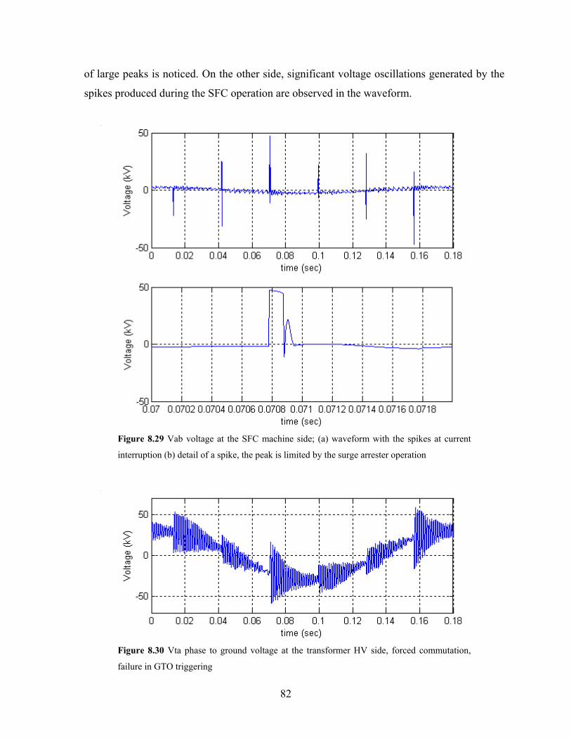
82
of large peaks is noticed. On the other side, significant voltage oscillations generated by the
spikes produced during the SFC operation are observed in the waveform.
Figure 8.29 Vab voltage at the SFC machine side; (a) waveform with the spikes at current
interruption (b) detail of a spike, the peak is limited by the surge arrester operation
Figure 8.30 Vta phase to ground voltage at the transformer HV side, forced commutation,
failure in GTO triggering

83
In Figure 8.30 the total magnitude of the voltage on the transformer terminals is much
smaller than the rated voltage because of the low operating frequency. In any case, to analyze
the possible harm of a voltage transient, not only the maximum peak but also other
parameters of the wave shape must be considered as it was explained in section 3.1. For the
voltage waveform on the HV side of the GSU of Figure 8.30 the relevant parameters are
shown in Table 8.2, they do not represent any harm to the transformer.
Table 8.2 Characteristic parameters of the transient waveforms over the GSU HV side during
forced commutation and failure in the triggering logic
Vtransf HV Peak (kV) Max change (kV)
Max rate (kV/µs)
Frequency (Hz)
Line-line 107.3 115 228 833
Line-ground 58.7 74 200 833
8.5 Validation of the Simulation Results
In electromagnetic studies based on computer simulations it is important to validate
the results and check the realism of the conclusions derived from the calculated values. There
are several items related with a study that have to be properly set in order to get results that
match the reality. These items generally are:
1- the models of the different elements present in the system. In this study the
component modeling was extensively discussed in chapter four,
2- the simulations must be done following the same operating procedures as the real
system, when no all the operating conditions can be checked, a study to detect the
cases producing the most relevant cases must be previously done
3- the software used for the simulations should be based on algorithms that provide
accurate results. In the case of electromagnetic studies in power systems, different
software packages are available to be used being most of them reliable and
appropriately tested [48].

84
Once the results are obtained from the computer simulation, it is also important to compare
the values against measurements in the real field. In the case of this study, the values and
waveforms obtained were matched with measurements taken in the field and presented in
other works [49], [50]. Although these studies were intended for different purposes, the
results and waveforms they provide allow for a comparison, and they basically support the
waveforms and values obtained here.
85
9 Analysis of the Results
The purpose of this chapter is to summarize the results obtained from the study and
the simulations. As it was previously stated in chapter three, there are three major effects of
power electronic system operating in a high voltage system. These three effects will be
analyzed in each of the following sections.
9.1 Harmonics
The presence of harmonics in current and voltage is expected when power electronic
devices are introduced in a power system because they create distortion of the voltages and
currents. Phase angle controlled converters, as the one used in the SFC under study, create a
harmonic spectra with values inversely decreasing with the increment of the harmonic order
[47]. This fact is observed as a general tendency in the waveforms obtained from this system,
but there are some exceptions as the thirteen-order harmonic that require an explanation. The
generation of harmonics is not only based on the SFC converter control but also on the
interaction between the different components of the system.
The operation of the SFC creates harmonics in the voltage and current that propagates
along the system. As was stated at chapter three, these harmonics can excite some resonances
existing in the system. This is precisely the effect that causes the increment in the thirteen
harmonic. In other words, the operation of the SFC creates a thirteenth harmonic that is
amplified by the resonance of the group of transformer, cable and synchronous machine. This
fact was first detected during the frequency scan test and confirmed with the time domain
simulations, where a more appropriate machine model for harmonic studies was used
showing also a resonance close to that 13th order. Although it is possible that exist some
differences in the exact value of some system parameters, the fact that certain “tuning” of the
power equipment increases some harmonic components was determined. Any possible
difference between the parameter used for the study and the actual value can change the
frequency at where the resonance takes place, and then the order and magnitude of the
harmonic. If the system parameters changes the resonances also varies. For example, in the

86
case of the cable disconnected from the transformer, the resonance move to a higher
frequency and almost disappear, but the phenomenon is similar.
The harmonic order that is amplified by the resonant effect changes with the system
frequency (machine speed). The resonant frequency at around 820 Hz corresponds to the 13th
harmonic at 60 Hz, but is switched to the 25th-29th order at 30 Hz. The main conclusion
regarding the harmonic presence in the system is the amplification due to resonance of some
of the harmonic components created by the SFC operation.
9.2 Overheating effects
When the SFC is operating, no load is applied to the transformer; therefore, the only
currents in the transformer are a reactive component due to the cable capacitance at 60 Hz,
which is relatively low, plus the transformer magnetizing current. This fact and the small
time that the SFC is used for the machine starting process can be enough to assure that the
GSU transformer will never experience overheating due to the SFC starting process.
Nevertheless, the calculation of the overheating effects by the harmonic current and voltage
will be presented in the following paragraphs.
The machine-accelerating regime is variable in frequency, voltage and current over
the GSU transformer. The frequency and voltage are related because the relation V/f is
maintained constant; therefore, lower frequencies are linked to lower voltages, and this
implies lower currents. With conservative criteria it is possible to calculate the losses under
non-sine wave conditions for the rated SFC rated operation at 60Hz being the losses at
different conditions smaller.
Equation (5-1) establishes that the transformer losses could be classified as load and
non-load ones. In the case of the transformer under study the losses are:
PNL= 127.3 kW
PLL= 952.4 kW
Under non- sinusoidal conditions while the non-load losses are related to the voltage
waveform, the load losses depends on the current waveform. For calculation of the losses
under distorted conditions it is important to know the values of the different terms of
equation (3-7). The first term is the DC losses and can be easily calculated given the value of

87
the winding resistance. In contrast, the separation between stray losses and eddy current
losses is not as simple. For the purpose of the calculation the percentage of eddy current and
stray losses was estimated based on typical values for this kind of transformers. The different
components of the loss under distorted conditions can be calculated according to factors
presented in chapter three. While the DC losses remain constant, the eddy current losses are
corrected by the K factor of equation (3-11) and the POSL by equation (3-10). The K factor
and the factor for correcting the other stray losses for the current Iatr result,
K= 0.17
KOSL= 7.6 e-3
On the other side, considering that the voltage distortion is not too big, condition (3-9) is
valid; the no-load losses under non-sinusoidal conditions are calculated by equation (3-8)
assigning half of them to eddy currents and half to hysteresis according to [20]. The results of
these calculations are presented in Table 9.1.
Table 9.1 Transformer losses for rated conditions and under the non-sinusoidal regime of the
SFC operating at rated speed
Type of loss Sine wave, rated V and I
SFC starting
PNL (kW) 127.3 128.9
PI2R (kW) 723.9 0.44
PEC (kW) 104.7 17.78
POSL (kW) 123.9 0.94
PLL(kW) 952.4 19.16
PTotal (kW) 1212.4 167.26
It is seen in the table that the load losses have decreased very much due to the small
current circulating in the transformer. Even though, the eddy current losses do not decrease in
the same proportion as the other load losses due to the relative importance of the harmonics.
The result PTotal shows that the total losses generated in the transformer under the operating
conditions imposed by the SFC are much smaller than the losses at rated conditions.

88
Therefore, it is possible to conclude that the magnitude of the harmonic regime during the
start process cannot cause transformer overheating. Moreover, as seen in Figure 5.1, the SFC
starting process last for a very short time compared to the transformer time constants, giving
less importance to any possible heating problem existing for that period of time.
9.3 Commutation Transients
The level of the transients found in the normal operation was not relevant and seems to
have more effect on the auxiliary starting bus than on the GSU transformer, synchronous
machine and related equipment. The presence of the generator is quite relevant sustaining the
voltage at the SFC output side. Moreover the windings of the synchronous machine and some
other devices present in the system like smoothing inductors filter the commutation
transients. No significant overvoltages due to commutation transients were found at the GSU
transformer terminals. In addition, the surge arresters and snubber circuits provide suitable
protection to the high voltage equipment.

89
10 Conclusions
The presence of harmonics is quite significant in the system under study. Some of the
harmonic components are amplified due to resonances existing between the different
equipment increasing the harmonic content over the level expected for the kind of equipment
employed. Nevertheless, the harmonic level is not relevant enough to create harm to any of
the equipment in the facility. The maximum voltage peak increased by the harmonic content
at the high voltage side of the GSU transformer does not create a voltage that can be
considered dangerous. The effect of overheating due to harmonics has no impact due to the
reduced values of the currents circulating during the starting period because the equipment is
working unloaded. Moreover, the starting process lasts for a short period over the complete
operation cycle of the different machines and equipment. Therefore, the impact over that
equipment is considerably reduced.
From this study we can conclude that most probably the SFC played no significant
role in the GSU transformer failures that have taken place in the past.

90
A Appendix A
The following data was not included in the model section but is required for the study.
A.1 Synchronous Machine Data
Table A.1 Synchronous machine reactances
Reactance Normal (%)
L (H) Saturated (%)
Synchronous direct-axis Xd 112.7 2.71e-03 99.5 Transient direct-axis X’d 28 6.74e-04 26 Subtransient direct-axis X”d 21 5.06e-04 18 Subtransient quadrature-axis X”q 23 5.54e-04 23 Negative sequence X2 22 5.30e-04 20 Zero sequence X0 12 2.89e-04
Table A.2 Synchronous machine time constants
Time constants (sec) Transient direct-axis T’d 2.4 Subtransient cc direct-axis T”d 0.052 Aperiodic 0.31

91
A.2 Transmission Cable Data
Due to its constructive characteristics the cable is modeled as three single-phase cables.
100.0 [ohm*m]Relative Ground Permeability:
Ground Resistivity:1.0
Earth Return Formula: Deri-Semlyen
0.0186 [m]
Cable # 1
.04514 [m]
.04754 [m]
.05114 [m]
0.0078 [m]
1 [m]
0 [m]
ConductorInsulator 1
SheathInsulator 2
On
20Maximum Order of Fitting for Prop. Func.:20Maximum Order of Fitting for YSurge:1.0E6 [Hz]Curve Fitting End Frequency:
Curve Fitting Starting Frequency: 5 [Hz]
Frequency Dependent (Phase) Model Options
Maximum Fitting Error for YSurge: 2 [%]2 [%]Maximum Fitting Error for Prop. Func.:
Travel Time Interpolation:
Figure A.1 Transmission Cable model
Line Model General Data Name of Line: cablemin Steady State Frequency [Hz]: 60.0 Length of Line [km]: 0.63 Number of Conductors:

92
A.3 SFC Control Circuit Diagram
Clear
1sT
zcros
EdgeDetector
gr2
gr6
*188.5
e-sT
e-sT
A
B
Compar-ator
A
B
Compar-ator
A
B
Compar-ator
e-sT
1.0
S Q
QR C
S Q
QR C
S Q
QR C
S Q
QR C
S Q
QR C
A
B
Compar-ator
S Q
QR C
gr5
gr4
1.0
gr1
gr3
D +
F
+
0.1
Irect
winh
A
B
Ctrl
Ctrl = 1
D +
F
+
D +
F
+
D +
F
+
cgr2
inh
winh
A
B
Ctrl
Ctrl = 1
cgr1
gr5
gr6
gr3
gr4
D +
F
+
e-sT
e-sT
1.57
0.0
G1 + sT
A
B
Ctrl
Ctrl = 1
A
B
Compar-ator
D +
F
+
*-1.0
*-1.0
*-1.0
D +
F
-
A
B
Compar-ator
0.0
zcros*1
Vscac
Vsabc
Vsbcc50.0
A
B
Compar-ator
0.7
0.6 ArcCosD +
F
- I
P
gr1
gr2
A
B
Compar-ator
vco
Va
Vb
Vc
PLL thetaMonostable
T
Figure A.2 SFC Control circuit: Rectifier control

93
cg3
cg4
cg5
cg2
cg6
1.0
Irect
cg1
A
B
Compar-ator
0.0
S Q
QR C
0.1
w
A
+
B+
C+
D +
E
+
F
+G
+
winpu
inh
winh
S Q
QR C
1.0
Monostable
T
winh
0.099
winpu
winpu
0.0
EdgeDetector S Q
QR C
1.0
A
B
Compar-ator
A
B
Compar-ator
EdgeDetector
alfa
Monostable
Tg2
g3
Monostable
T
g4
g5
Monostable
Tg6
wu
-0.2
-0.2
-0.2
Et1
-0.2
-0.2
Et3
Et4
Et5
-0.2
Et6
A
B
Compar-ator
A
B
Compar-ator
A
B
Compar-ator
A
B
Compar-ator
S Q
QR C
Monostable
TMonostable
T
G1 + sT
1.0
Monostable
Tg1
A
B
Compar-ator
1.570.7
D +
F
+
G1 + sT D +
F
+
A
+
B
+C
+D +
E
+
F
+
Et2
A
B
Compar-ator
B
+C
+D +
E
+
F
+G
+
Figure A.3 SFC Control circuit: Rectifier-Inverter control circuits

94
g5
0.0alfa
anr
5.236
D +
F
+
-1.047
-4.188
D +
F
+
3.1416
-3.1416
D +
F
+
4.188
2.095
-2.095
D +
F
+
-5.236
1.047
winh
D+
F
-
S Q
QR C
S Q
QR C
S Q
QR C
S Q
QR C
S Q
QR C
g4
S Q
QR C
g6
g1
S Q
QR C
g2
S Q
QR C
g3
1.0
cg4
cg5
cg6
cg1
cg2
cg3
S Q
QR C
S Q
QR C
S Q
QR C
1.0
g4
g5
g6
g1
g2
g3
EdgeDetector
EdgeDetector
EdgeDetector
EdgeDetector
EdgeDetector
A
B
Compar-ator
A
B
Compar-ator
A
B
Compar-ator
A
B
Compar-ator
A
B
Compar-ator
A
B
Compar-ator
A
B
Compar-ator
A
B
Compar-ator
A
B
Compar-ator
A
B
Compar-ator
A
B
Compar-ator
EdgeDetector
S Q
QR C
EdgeDetector cg1
EdgeDetector cg2
D +
F
+ cg3Edge
Detector
cg4
cg5Edge
Detector
EdgeDetector cg6
u
EdgeDetector
EdgeDetectorinh
TIME
Figure A.4 SFC Control Circuit: Inverter control

95
A.4 SFC Power Circuit Diagram
Et1 Et5
Vbc
Et3
Va
Vab
Ibto
Vis
Vab
0.017
T
T
Vsa
Vsb
Vsc
Isa
gr1 gr3
gr4
gr5
gr6
Vna
Vna
T
gr2
Isa2
0.001
0.001
0.001
Vsa
Irect
Vsab
0.001
0.006
T
Iatog1
G
g3
G G
g5
g4 g6
G
g2
100.0
0.006
Isc2
0.006
Icto
0.001435
A
B
C
T T G
Irect
0.017
Vsbc
Vsab
Vsc
a
Et6 Et2 Vc
Vb
G
Va
Et1
Vac
Vis
Et4
A
B
C
A
B
C
24.5 [MVA]
13.8 16.5
#1 #2
Figure A.5 SFC Power Circuit: this portion shows the SFC itself and the auxiliary source

96
w
0.0036
0.0036
0.01
0.01
0.010.000707
0.000707
Ibto
Pg
Te
Tm
Iag
Tm
w
ang
anglea
0.0
01
0.0
01
0.0
01
Pm
Qg
Te
anr
mposA B C
A B C
Iato 0.0007070.0036
0.001
0.001
0.001
Vtlbc
Vtlc
a
Vtbc
Vtc
a
Vta
Vtb
Vtc
Ibtr
Iatr
Vtab
0.001
Vtlab
Ictr
0.001
Ict
Ibt
Iat
#1 #2
Power
A
B
P
Q
0.001
0.001
0.001#1 #2
0.001
C1cablemin3
VcababVcabaC1cablemin2
C1cablemin3
C1cablemin2
C1cableminC1cablemin
cablemin
0.0
00
50.0005
0.0003
0.0003
0.0003
0.0005 0.0
05
0.0
05
0.0
05
0.0
1.05
#1 #2
Sync1
EfIf
Tm w
w
Te
Tm
A
B
C
cablemin3
( SyncM
/c)M
ultimass
Te
Wra
dTm
cablemin2
Icto
Figure A.6 SFC Power Circuit: this portion shows the synchronous machine, GSU transformer, and HV cable

97
B Appendix B This Appendix shows additional waveforms for the following operation cases:
1. Rated operating conditions –base case
2. Reduced load condition
3. Reduced speed condition
4. Operation without HV transmission cable
5. Forced commutation mode
6. Snubber circuit not operative
7. Snubber circuit operative: natural and forced commutation
8. Failure in the firing sequence
The way the waveforms are presented is always the same staring from the HV side of
the transformer to the auxiliary bus of the station. The voltage waveforms are presented first
followed by the current waveforms.
B.1 Rated operating conditions –base case
Figure B.1 Voltage waveforms at rated conditions at the transformer HV terminals (a) line-line (b) line-ground

98
Figure B.2 Voltage waveforms at rated operating condition (a) Vcabab Line –line voltage at the cable open terminal (b) Vtlab Line –line voltage at the transformer LV terminal. The shape is the same as the HV side, but the harmonic content is smaller (c) Va Line – ground voltage at the converter output side (d) Vab Line – line voltage at the SFC converter output side
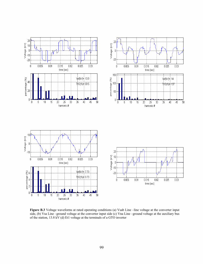
99
Figure B.3 Voltage waveforms at rated operating conditions (a) Vsab Line –line voltage at the converter input side, (b) Vsa Line –ground voltage at the converter input side (c) Vna Line –ground voltage at the auxiliary bus of the station, 13.8 kV (d) Et1 voltage at the terminals of a GTO inverter

100
Figure B.4 Current waveforms at rated operating conditions (a) Iatr Phase current at the LV winding of the main transformer, in the delta (b) Itla Magnetizing current at the LV branch of the main transformer (c) Iat Line current at the LV side of the GSU transformer (b) Iag Synchronous machine input current

101
Figure B.5 Current waveforms at rated operating conditions (a) Iato SFC output current, there is no major difference with Isa2, the input current of the SFC (b) Irect current at the DC interface of the SFC (c) Isa SFC input current at the primary side of the auxiliary transformer, 13.8kV

102
B.2 Reduced load condition
Figure B.6 Voltage waveforms for reduced load condition (a) Vtab Line –line voltage at the transformer HV terminal. The harmonic content is reduced respect to the base case (b) Vab Line – line voltage at the SFC at the machine side (c) Vtlab (d) Vsab Line – line voltage at the converter input side, 16.5kV

103
Figure B.7 Current waveforms for reduced load conditions (a) Iat Line current at the LV side of the main transformer (b) Iato the SFC output current at 16.5 kV

104
B.3 Reduced Speed condition, ω=0.5*ωr
Figure B.8 Voltage waveforms at reduced speed operation (a) Vtab line-line voltage at the transformer HV terminals (b) Vtlab line-line voltage at the transformer low voltage terminals (c) Vsab line-line voltage at the SFC input (d) Vsa line-phase voltage at the SFC input

105
Figure B.9 Current waveforms at reduced speed operation (a) Iat line current at the transformer LV side (b) Iatr phase current at the transformer LV side (c) Iag Line current at the generator (d) Iato SFC output current

106
B.4 Operation without HV transmission cable
Figure B.10 Voltage waveforms for operation without HV cable (a) Vtab Line –line voltage at the transformer HV terminal (b)Vtlab Line –line voltage at the transformer LV terminal (c) Vab Line –line voltage at the SFC output (d) Vsab Line – line voltage at the SFC input side, 16.5 kV

107
Figure B.11 Current waveforms for operation without HV cable (a) Iag current taken by the synchronous machine (b) Iatr Current at the LV winding of the main transformer, inside the triangle connection

108
B.5 Forced Commutation Mode
Figure B.12 Voltage waveforms at forced commutation (a) Vtab line-line voltage at the transformer HV side (b) Vtlab line-line voltage at the transformer LV side (c) Vab Line line voltage at the SFC output (d) Et3 Voltage at the terminals of an inverter GTO

109
Figure B.13 Voltage waveforms during forced commutation (a) Vsab Line-line voltage at the SFC input side (b) Vna Line-ground voltage at the primary side of the auxiliary transformer 13.8 kV
Figure B.14 Current waveforms during forced commutation operation (a) Iat Line current at the transformer LV side (b) Iag current taken by the generator

110
Figure B.15 Current waveforms at forced commutation operation (a) Iato SFC output current, it is observed the absence of higher order components which are absorbed by the generator (b) Irect Current in the DC interface (c) Isa current at the SFC input (d) Isa2 current at the primary side of the auxiliary transformer, 13.8 kV

111
B.6 Snubber circuit not operative
Figure B.16 Voltage waveforms for the study of the commutation transient without snubber circuit (a) Vtab line-line voltage at the transformer HV side (b) Vta line-ground voltage at the transformer HV side (c) Vab line-line voltage at the SFC output (d) Va line-ground voltage at the SFC output side (e) Vsab line-line voltage at the SFc input side (f) Vsa line-line voltage at the SFC input side

112
B.7 Snubber Circuit Operative
B.7.1 Natural Commutation
Figure B.17 Voltage waveforms at natural commutation for the study of the commutation transient with snubber circuit in operation (a) Vab line-line voltage at the SFC output (b) Va line-ground voltage at the SFC output (c) Vsab line-line voltage at the SFC input side (d) Vsa line-ground voltage at the SFC input side

113
B.7.2 Forced Commutation
Figure B.18 Voltage waveforms at forced commutation for the study of the commutation transient with snubber circuit in operation (a) Vtab line-line voltage at the HV side of the transformer (b) Vta line-ground voltage at the HV side of the GSU transformer (c) Vab line-line voltage at the SFC output (d) Va line-ground voltage at the SFC output (e)Vis voltage at the DC interface

114
B.8 Failure in the Firing Sequence
Figure B.19 Voltage waveforms for the study of the transient produced by a miss-synchronization of the firing pulses (a) Vtab line-line voltage at the transformer HV side (b) Vta line-ground voltage at the transformer HV side (c) Vtlab line-line voltage at the transformer LV side (d) Vab line-line voltage at the SFc output (e) Va line-ground voltage at the SFC output (f) Enlargement of Vab to observe the details of the spike

References
[1] G. Magsaysay et al., “Use of a Static Frequency Converter for Rapid Load Response in
Pumped-Storage Plants,” IEEE Trans. Energy Conversion, Vol. 10, No. 4, December
1995
[2] R. Rudenberg, Transient performance of Electric power systems, M.I.T., London, UK,
1970
[3] A. Greenwood, Electrical Transients in Power Systems 2nd ed., Wiley, New York, 1991
[4] Elkins et al, Transients During 138KV SF6 Breaker Switching of Low Inductive
Currents. IEEE Trans. on Industry Applications, vol. 29, no.4, July 1993.
[5] CIGRE Working group 33/13-09, “Very Fast Transient Phenomena Associated with Gas
Insulated Substations”, CIGRE Report 33-13, 1988
[6] Y. Shibuya et al, “Effects of Very Fast Transient Overvoltages on Transformer”, IEE
Proc. Gener. Transm. Distrib., vol. 146, no. 4, July 1999
[7] IEEE working group report, “Estimating lightning performance of transmission lines. II.
Updates to analytical models”, IEEE Transactions on Power Delivery, vol.8, no.3, July
1993, pp.1254-67
[8] J. Arrillaga, D. Bradley, P. Bodger, Power System Harmonics, John Wiley & Sons, 1985
[9] A. Arsoy et al. Modeling and Simulation of Power System Harmonics, IEEE Press,
Piscataway NJ, 1998
[10] R. Dugan et al., Electrical Power Systems Quality, McGraw-Hill, 1996
[11] R. Tessendorf, “Application of Arresters and Surge Protective Devices to DC Drives”,
Conf. Rec. of 1986 Annual Pulp and Paper Industry Technical Conference, IEEE, pp.66-
70, 1986
[12] K. Harada et al, “Optimum Design of RC Snubbers for Switching Regulators”, IEEE
Transactions on Aerospace and Electronic Systems, vol. AES-15, no. 2, March 1979
[13] J. Olivier, G. Stone, “Implications of the Application of Adjustable Speed Drive
Electronics to Motor Stator Winding Insulation”, IEEE Electrical Insulation Magazine,
pp.32-36, 1995

116
[14] C. Lanier, “A novel Technique for the Determination of Relative Corona Activity within
Inverter-Duty Motor Insulation Systems Using Steep-Fronted Voltage Pulses”, Conf.
Record of the 1998 Int. Sym. On Electrical Insulation, pp. 229-236, 1998
[15] CIGRE Joint Working Group 12/14.10, “HVDC converter transformers”, CIGRE 1996:
12-202
[16] X. Dong et al., “Simulation of switching, SFC, and lightning transients in Mingtan
pumped storage plant (Final Report)”, unpublished work
[17] S. P. Kennedy, C.L. Ivey, “Application, Design and Rating of Transformers Containing
Harmonic Currents”, Pulp and Paper Industry Technical Conference, 1990, Conference
Record pp: 19-31
[18] E. Fuchs, R. Fei, “A New Computer-Aided Method for the Efficiency Measurement of
Low-loss Transformers and Inductors Under Non-sinusoidal Operation”, IEEE Trans.
On Power Delivery, Vol. 11, No.1, January 1996
[19] E. Emmanuel, X. Wang, “Estimation of loss of life of Power Transformers Supplying
Non-linear Loads”, IEEE Trans. On Power Apparatus and Systems, Vol PAS-104, no.3,
March 1985
[20] IEEE Transformers Committee, “Standard Test Code for Liquid-Immersed Distribution,
Power and Regulating Transformers”, ANSI/IEEE std. C57.12.90, 1987
[21] M. A. Masoum, E. F. Fuchs, D. J. Roesler, “Impact of Nonlinear Loads on Anisotropic
Transformers”, IEEE Trans. On Power Delivery, October 1991, Vol. PWRD-6, pp.
1781-1778
[22] A. Kelley et al. “Transformer Derating for Harmonic Currents: A Wide-Band
Measurement Approach for Energized Transformers”, IEEE Trans. On Industry
Applications, vol. 35, no. 6, Nov/Dec 1999
[23] IEEE Transformers Committee, “IEEE Recommended Practice For Establishing
Transformer Capability When Supplying Nonsinusoidal Load”, Std C57.110-1998, 1998
[24] Underwriters Laboratory, “Dry Type General Purpose and Power Transformers”,
Standard UL 1561, Apr. 22, 1994
[25] D. Yildrim, E. Fuchs, “Measured Transformer Derating and Comparison with Harmonic
Loss Factor (FHL) Approach”, IEEE Trans. On Power Delivery, vol. 15, no.1, Jan 2000

117
[26] A. Delaiba et al., “The Effect of Harmonics on Power Transformers Loss of Life”,
Proceedings of the 38th Midwest Symposium on Circuits and Systems, 1995, pp 933-
936 vol.2
[27] P. Krause, Analysis of electric Machinery, McGraw-Hill, 1986
[28] B. K. Bose, Power Electronics and AC Drives, Prentice-Hall, New Jersey, 1986
[29] U. de Martinis, et al., “On the Evaluation of the Harmonic Impedances in AC/DC
Systems,” ICHPS V Int. Con. on Harmonics in Power Systems. IEEE, pp.102-6. New
York, 1992
[30] J. Eggleston at al. “Harmonic Norton Equivalent of the Synchronous Generator,” Journal
of Electrical and Electronic Eng., Australia, Vol. 7, No. 1, March 1987
[31] P. Hart, J. Bonwick, “Harmonic Modeling of Synchronous Machines,” IEE
Proceeedings, vol. 135, Pt. B, No. 2, March 1988
[32] X. Zhang, E. Handschin, “Frequency-Dependent Simple Harmonic Model of
Synchronous Machines,” IEEE Power Engineering Review, vol.20 No.5, May 2000
[33] E. W. Kimbark, Power System Stability, Vol. 3, Synchronous Machines, IEEE Press,
New York, 1995.
[34] P. Anderson, A. Fouad Power System Control and Stability, Iowa State University Press,
1986
[35] J. Martinez-Velasco, “ATP Modeling of Power Transformers,” European EMTP-ATP
Users Group News, pp. 63-76, Aug-Nov 1998
[36] W. Dugui, X. Zheng, “Harmonic Model of Power Transformer”, 1 Harmonic model of
power transformer”, Proceedings. POWERCON '98. Int. Con. Power System
Technology, Vol. 2, pp. 1045 –1049, 1998
[37] Task Force on Harmonic Modeling & Simulation “Modeling and Simulation of the
Propagation of Harmonics in Electric Power Networks – Part I”, IEEE Trans. Power
Delivery, Vol. 11, No. 1, January 1996
[38] Manitoba HVDC Research Centre, EMTDC Theory Manual, Winnipeg, 1994
[39] T-H. Liu et al. “Modeling and Performance of a Static Frequency Converter Starting a
300MVA Synchronous Machine”, Electric Power Systems Research, vol.37, pp.45-53,
1996.
118
[40] K.V. Rao et al., “Static Frequency Converter Starting of Microsynchronous Motor,”
Journal of the Institution of Engineers (India), Part El, vol.64, pp.241-7, April 1984
[41] B. Mueller et al. “Static Variable Frequency Starting and Drive System for Large
Synchronous Motors”, Conf. Rec. IEEE/IAS Annual Meeting, pp. 429-438, 1979
[42] J. Murphy, F. Turnbull, Power Electronic Control of AC Motors, Pergamon Press,
Oxford, 1988
[43] Le-Huy et al., “Microprocessor Control of a Current-fed Synchronous Motor Drive”,
Report from the IEEE/IAS Annual Meeting, pp. 873-880, 1979
[44] R. Krishnan, Electronic Control of Machines, Virginia Tech, Blacksburg VA, 1999
[45] A. Trzynadlowski, “Introduction to Modern Power Electronics”, John Wiley &Sons,
1998
[46] G. Heydt, “Power System Quality”, Stars in a Circle Publications, 1991
[47] D. Rice, “Adjustable Speed Drive and Power Rectifier Harmonics-Their Effect on Power
System Components”, IEEE Transactions on Industry Applications, vol. IA-22, no.1, pt.
1, Jan-Feb 1986, pp 161-77
[48] L. X. Bui, G. Morin, “Some Experiences in Power System Simulation Using
Electromagnetic Transient Programs”, Canadian Conference on Electrical and Computer
Engineering, Vol. 2, pp 647–650, 1996
[49] T-H. Liu et al. “Modeling and Harmonics Elimination for a Static Frequency Converter
Driving a 300MVA Synchronous Machine”, Proc. of the IEEE Int. Symposium on
Industrial Electronics ISIE '96, IEEE. Part vol.2, pp.602-7, New York, 1996
[50] J-C. Chiang et al. “Mitigation of Harmonic Disturbance at Pumped Storage Power
Station with Static Frequency Converter”, IEEE Tans. Energy Conversion, Vol.12, No.
3, Sep. 1997

119
Vita
Sebastian Rosado was born in Rosario, Argentina, on March 14th 1968. He got his
electrical engineering degree from the National University of Rosario on March 1994. From
1994 to 1999 he worked as an electrical engineer at Acindar, a steel making company in
Argentina. His work there dealt with the generation and distribution electric system of the
company, a major consumer of electricity. From 1991 to 1999 he also worked as an assistant
and teacher at the Polytechnic Institute of the National University of Rosario. On August
1999 he came to Virginia Tech to pursue his Masters degree in Electrical Engineering.


![GAS RANGES ELECTRIC STATIC / CONVECTION OVENS · GE508D[1] 8 Open Burners + Electric Static Oven. GE508C[1] 6 Open Burners + 300 mm Griddle + Electric Static Oven. GE508B[1] ... adjustable](https://img.dokumen.tips/doc/110x75/5fb98b51c920dd0fde02e693/gas-ranges-electric-static-convection-ovens-ge508d1-8-open-burners-electric.jpg)