Embed Size (px)
Citation preview
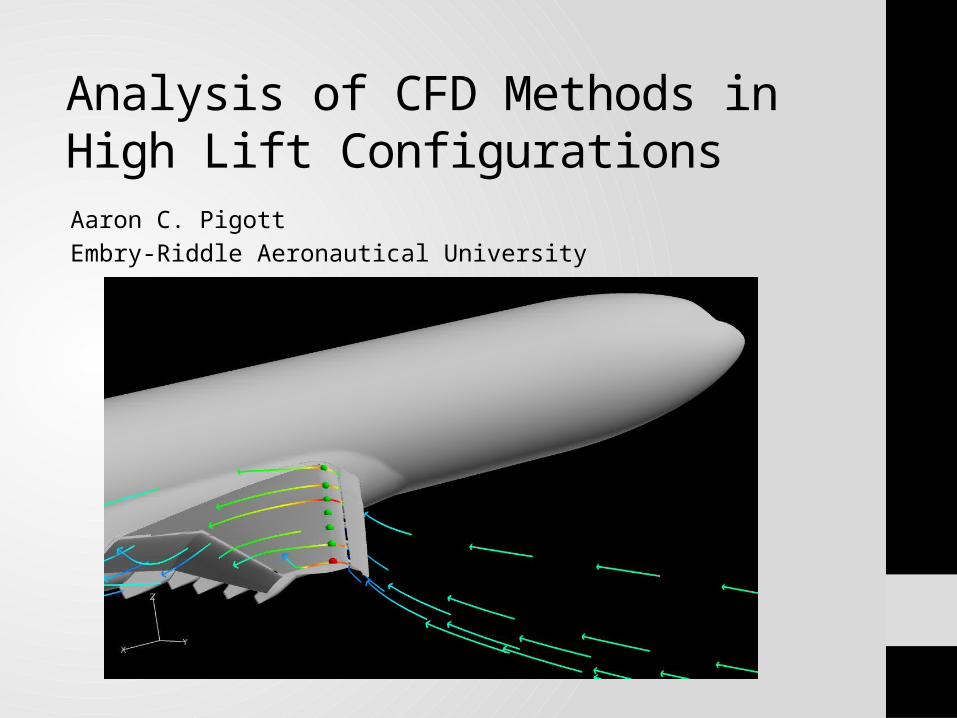
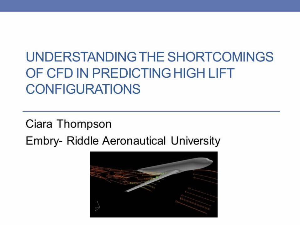
Analysis of CFD Methods in High Lift ConfigurationsAaron C. PigottEmbry-Riddle Aeronautical University
Introduction and Overview• Introduction• AIAA HighLift Workshop under Dr. Earl Duque and Dr. Shigeo
Hayashibara• Goal: CFD Validation in a High Lift Configuration by comparing
CFD to Wind Tunnel data• Specifically: Validation using velocity profile comparisons
• Overview• The Model• Experimental Setup• CFD Setup• Data• Points of Interest• Summary
2

The Model• KH3Y geometry, DLR-F11 model• Designed to represent wide-body commercial aircraft landing• Designed for the European High Lift Project
3
SlatWing
Fuselage
Flap
SlatWing
Fuselage
Flap
Flap Tracks
Slat Tracks
SlatWing
Fuselage
Flap
Flap Tracks
Slat Tracks
Pressure Tube Bundles
FlapFlap
Slat Track
Flap Track
Slat Track
Flap Track
SlatPressure Tube BundleSlat
Slat
Flap
Configuration 2Configuration 2Configuration 4Configuration 4Configuration 5Configuration 5
From AIAA 2012-2924
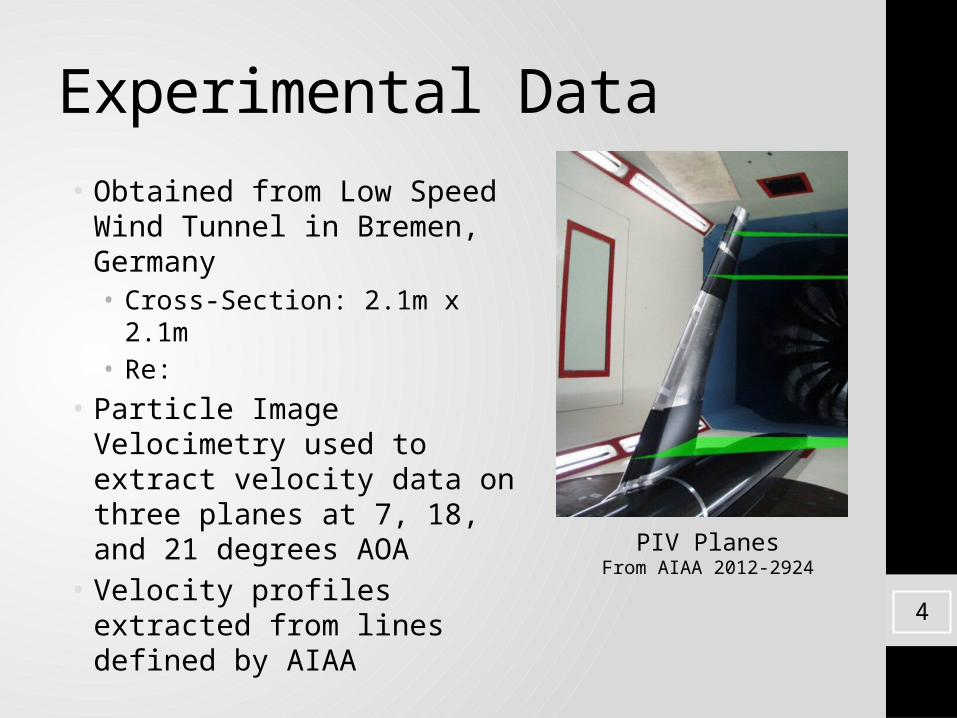
Experimental Data• Obtained from Low Speed Wind
Tunnel in Bremen, Germany• Cross-Section: 2.1m x 2.1m• Re:
• Particle Image Velocimetry used to extract velocity data on three planes at 7, 18, and 21 degrees AOA
• Velocity profiles extracted from lines defined by AIAA
PIV PlanesFrom AIAA 2012-2924
4
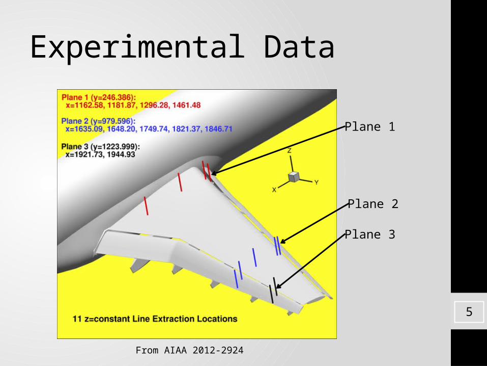
Experimental Data
5
Plane 1
Plane 2
Plane 3
From AIAA 2012-2924
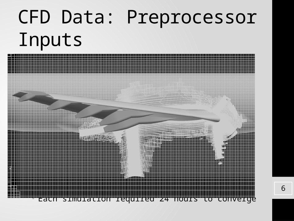
CFD Data: Preprocessor Inputs• Preprocessing performed by Dr. Earl P. N. Duque• Spalart-Allmaras Turbulence Model• Meshing: Overset Grid• Series of overlayed structured grids• 69 million grid points
• Solver: Overflow Code• Reynolds-Averaged Navier-Stokes solver by Pieter Buning, NASA
Langley
• Simulations performed on Cray XE6 system• 1024 compute cores • Each simulation required 24 hours to converge 6

CFD Data: Testing• Extract u-velocity profile from 11 locations on wing at 7, 18.5, and
21 degrees AOA• CFD: Extraction lines at same locations as experimental
7
From AIAA 2012-2924
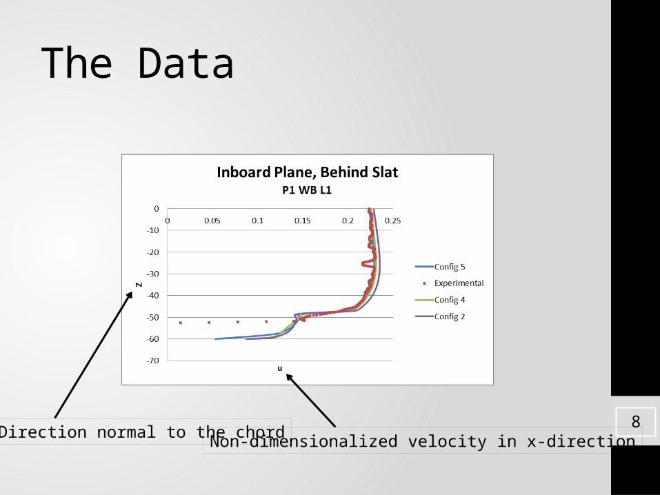
The Data
Non-dimensionalized velocity in x-directionZ: Direction normal to the chord 8
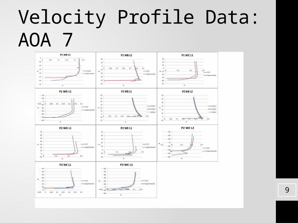
Velocity Profile Data: AOA 7
9
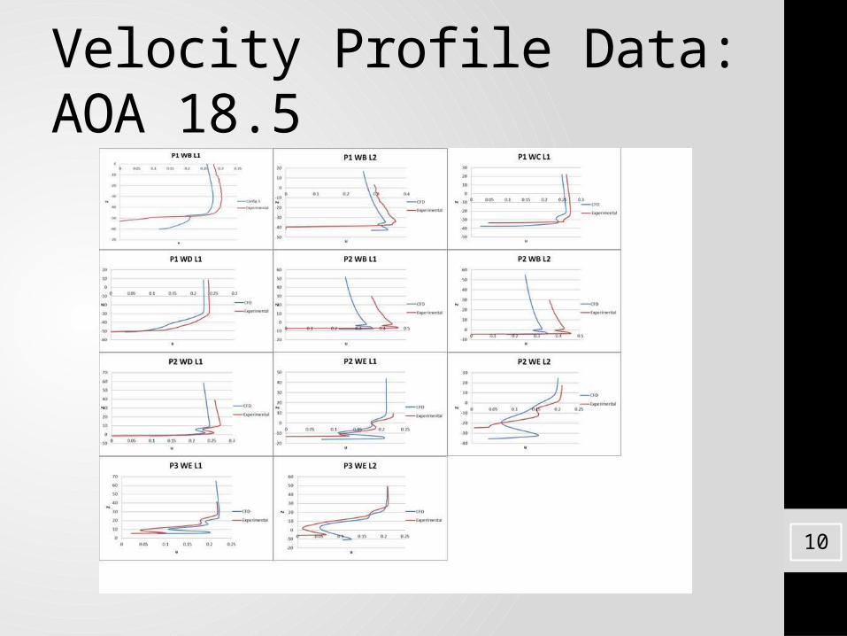
Velocity Profile Data: AOA 18.5
10

Velocity Profile Data: AOA 21
11

Points of Interest• Small divots appear in experimental data velocity profiles• As angle of attack increases, correlation between CFD and PIV
data decreases• A few locations show very little correlation between CFD and
Experimental velocity data (Plane 2 Window B)• CFD does not detect reverse flow shown in Plane 2 window D
12
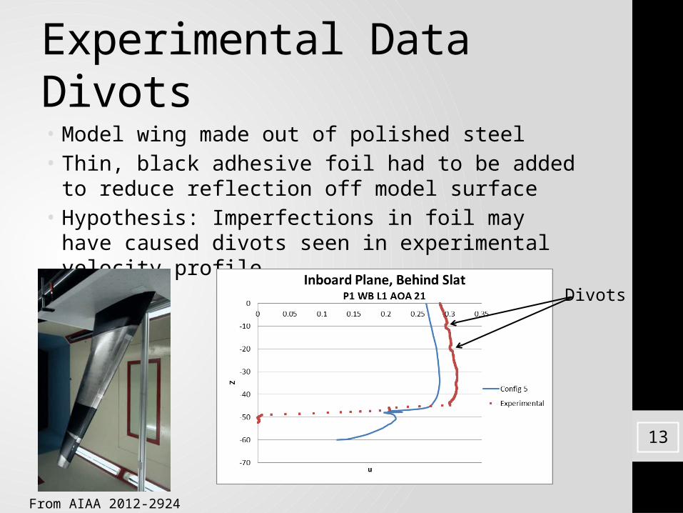
Experimental Data Divots• Model wing made out of polished steel• Thin, black adhesive foil had to be added to reduce reflection
off model surface• Hypothesis: Imperfections in foil may have caused divots seen
in experimental velocity profile
Divots
13
From AIAA 2012-2924

Increasing AOA, Decreasing Correlation
14

AOA 21 Plane 1 Window BExperimental FieldView
15
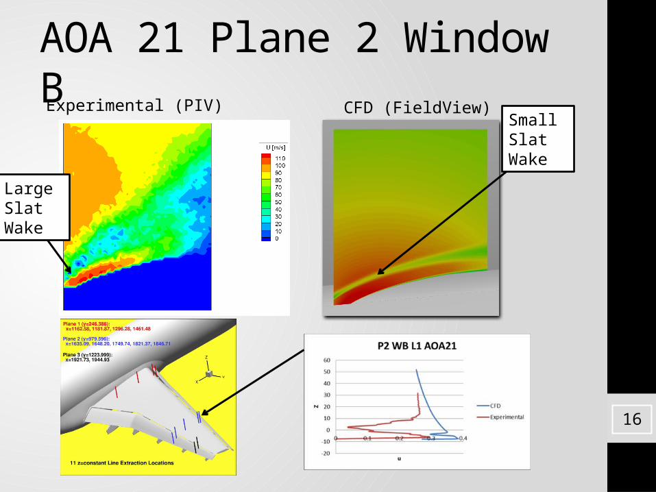
AOA 21 Plane 2 Window BExperimental (PIV) CFD (FieldView)
16
Large Slat Wake
Small Slat Wake
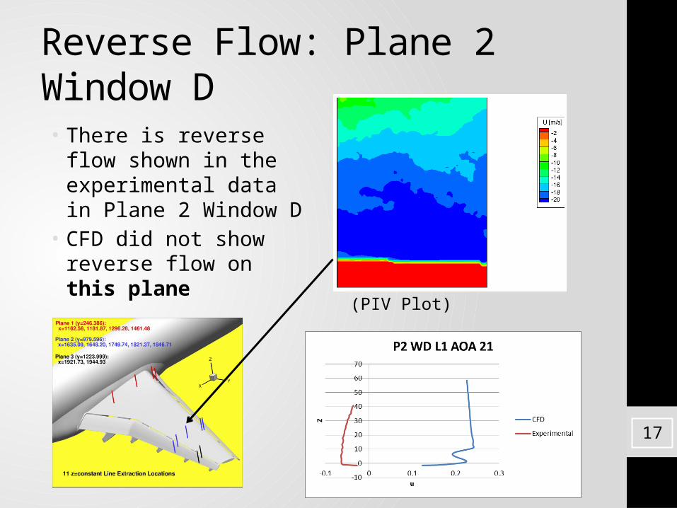
Reverse Flow: Plane 2 Window D
• There is reverse flow shown in the experimental data in Plane 2 Window D
• CFD did not show reverse flow on this plane
(PIV Plot)
17
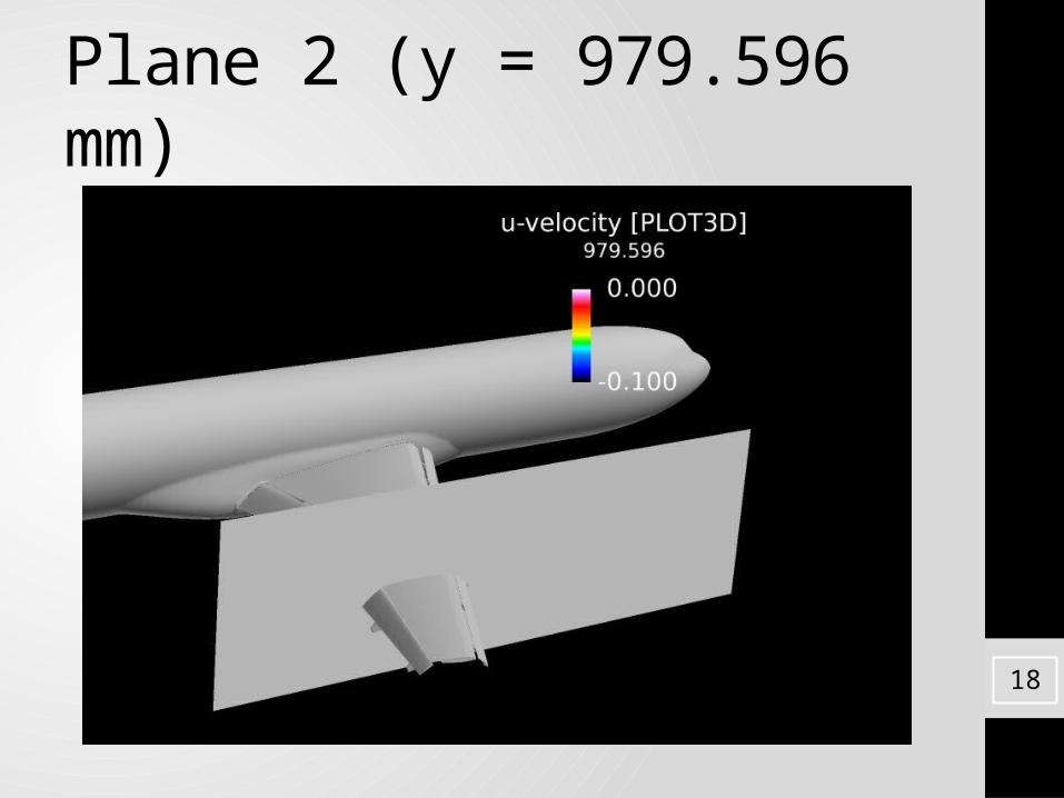
Plane 2 (y = 979.596 mm)
18
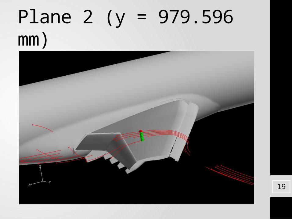
Plane 2 (y = 979.596 mm)
19
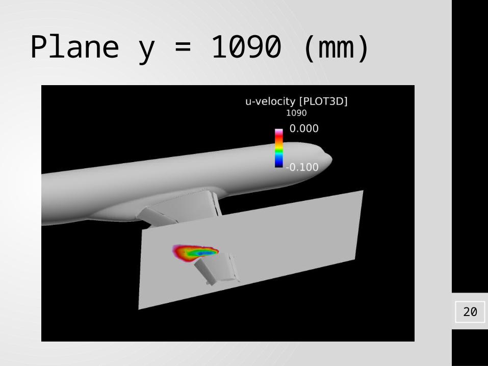
Plane y = 1090 (mm)
20

Plane y = 1090 (mm)
21

Plane y = 1090 (mm)
Slat Track and Pressure Tube Bundle
22

Reverse Flow Shift Outboard• CFD shows airflow separation 100mm further outboard than
the PIV data• The shift is likely due to model pressure tube representation
DLR-F11 Pressure Tubes
CFD Model Pressure Tubes
23
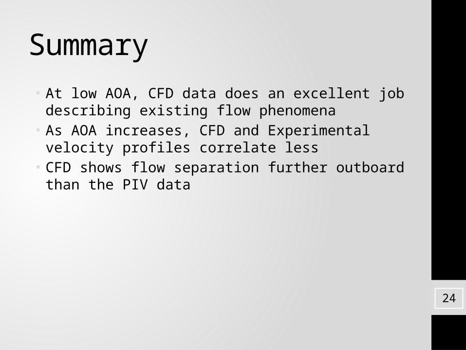
Summary• At low AOA, CFD data does an excellent job describing existing
flow phenomena• As AOA increases, CFD and Experimental velocity profiles
correlate less• CFD shows flow separation further outboard than the PIV data
24

Acknowledgements• CFD images were created using FieldView as provided by
Intelligent Light through its University Partners Program
• Simulations were performed by Dr. Earl P.N. Duque, Manager of Applied Research, Intelligent Light
Dr. Shigeo Hayashibara, ERAU CFD Research Group
25
26
Questions?
27

Appendix• To non-dimensionalize the experimental data, the velocity was
divided by the speed of sound• The speed of sound for this experiment:
28
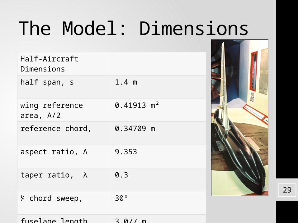
The Model: DimensionsHalf-Aircraft Dimensions
half span, s 1.4 m
wing reference area, A/2 0.41913 m²
reference chord, 0.34709 m
aspect ratio, Λ 9.353
taper ratio, λ 0.3
¼ chord sweep, 30°
fuselage length, 3.077 m
High Lift System
Slat Deflection (Full Span) 26.5°
Flap Deflection (Full Span) 32.0°
29

AOA 7 Data w/ All Configs
30
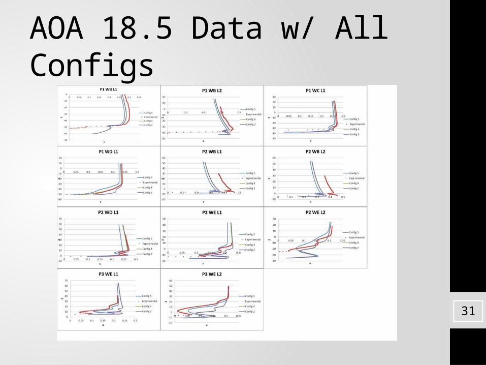
AOA 18.5 Data w/ All Configs
31

AOA 21 Data w/ All Configs
32
Why do we care about Velocity Profiles?• Velocity profiles paint a picture of airflow at different locations
on the surface of the wing. They point out flow phenomena such as separation.
33
Why was S-A turbulence model used?• Designed specifically for aerospace applications• Shown to give good results for boundary layers subjected to
adverse pressure gradients• Solves a modeled transport equation for kinematic eddy
viscosity
34
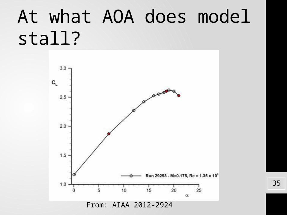
At what AOA does model stall?
From: AIAA 2012-2924
35