Analysis of Censored Cost or HealthOutcomes Data

Part IStatistical Methods for Censored Medical Cost

Heejung Bang, PhD

Division of Biostatistics and Epidemiology

Department of Public Health

Weill Medical College of Cornell University

1

OUTLINE

• Background

• Statistical issues in medical cost data analysis

• Statistical methods: naive vs. valid

• Regression and cost-effectiveness analysis (CEA)

• Examples: MADIT II, SEER, Marketing

• Research summary and other issues not covered

• Conclusions and discussions

• Appendix: Equivalences among well known estimators

2

General Background

• Until the late 1970s, so-called ‘open checkbook era’.

• From the late 1980s, an aggressive, concerted voice started to askfor control of health care costs and fiscal accountability inmedicine.

• Medical cost is important data. Check your bills for health care.

• Sky-rocketing costs but limited resources.

• Practitioners, economists and statisticians’ roles in collection,analysis and interpretation of medical costs started to beemphasized.

• Costs are conventionally evaluated to assess its economicimplication as a secondary outcome.

3

Methodological Background

• Incompleteness (due to censoring) is a key feature of mostsurvival data.

• There are numerous well established statistical methodologiesand algorithms exist for analyzing censored survival data (e.g.,Kaplan-Meir (KM), Cox model).

• Survival time and lifetime medical cost are similar.

• However, ‘informative censoring’ in medical cost invalidates theuse of most standard analytic tools suited for survival data.

• Valid methods for analyzing censored medical costs have beenactively developed (since 1st discovery by Lin et al. 1997).

Remark: medical cost, quality-adjusted lifetime (QAL) and customerlifetime value have similar mathematical properties.

4

Statistical Issues

• Mean vs. Median, Regression, CEA.–Mean: Most common. Total cost can be derived from mean, notmedian. CEA uses mean.–Median (or quantiles): More robust to outliers, for skewed data,popular in Econometrics.Remark: Today’s talk is mostly about ’MEAN’ estimation andextensions to other contexts will be made.

• ‘Informative censorship’ (or induced dependent censorship) dueto positive correlation between total cost at event and total costat censoring even if event time and censoring time areindependent (Lin et al. 1997).— In fact, problems of informative censoring occur in caseswhere the process of interest (e.g., cumulative cost) is increasingover time and its observation is stopped due to the occurrence of

5

a possibly dependent terminal event (Strawderman 2000).

• Thus, most standard statistics are not valid (e.g., sample mean,t-test, ordinary least squares, KM estimates, Log-rank test, andCox model, etc.).

• Fundamental methodological idea: inverse probability weighting(IPW) in order to account for informative (right) censoring forconsistent estimators and semiparametric efficiency theory forefficient estimators.— IPW was originated from survey sampling (Horvitz &Thompson 1952), later widely used in biostatistics (e.g., missingdata and causal inference).

• Applicable to biostatistics, epidemiology, health economics,health outcomes research, marketing.

6

Graphical illustration of informative censoring (Figure 2 from Lin 2003)

7

Examples of informative censoring in real life

• time of heart attack (event) and time of car accident (censoring)are likely independent. However, money you have accumulated inyour saving’s account at these times will be positively correlated(because both depend on the savings rate and how long).

• time of death (event) and time of divorce (censoring) are likelyindependent. However, money a wife will get from her richhusband at these times will be positively correlated.

Heuristic formula for informative censoringcov(βi ∗ Ti, βi ∗ Ci) 6= 0 even if cov(Ti, Ci) = 0,

where βi is random.

If βi is a constant, two costs become independent.

8

Notation

• T ∗=a subject’s survival time or the time before all the cost dataare available. T = min(T ∗, τ) with the max follow-up time τ .

• M(t)=the medical cost up to time t. Let M(T ) ≡ M .

• Our goal is estimating E(M)=expected value of M .

• C=time to censoring, assumed to occur independently of allothers (i.e., completely at random).

• Time intervals/partitions: [0, τ) ≡ [a1, a2) ∪ · · · ∪ [aK , aK+1) ispartitioned into K sub-intervals [ak, ak+1) for k = 1, · · · ,K (say,by year or month).

• So partitioned costs are Mk = M(ak+1)−M(ak).

• S(t) = P (T > t) and K(t) = P (C > t), where S(t) can beestimated by the standard KM estimator and K(t) can be

9

estimated by switching ∆ and 1−∆.

• Observed data for each individual are:[X = min(T,C), ∆ = I(T ≤ C), {M(u), u ≤ X},Z], where Z is aset of covariates and I is an indicator function.

Remarks:–Z can be used in regression or for improving efficiency.–S(t) and K(t) can be estimated by the Cox model andBrowslow estimator if C does not occur completely at random.–M(u) is likely to be realized in a finite fashion.–If the cost history is not recorded, we only get to see theterminal cost M(X) for each individual.–those who experience the event of interest before being censoredhave M = M(T ) = M(X).– M will denote M(T ) or M(X) to save notations when thecontext is clear. (sorry!!)

10

Statistical methods: Naive approaches (oldies butnot goodies)

• For complete cost data (i.e., no censoring), no problem! You canuse any methods suited for uncensored or censored data.

• Under right censoring, 3 naive approaches are:1. Full sample mean

∑ni=1 Mi

n : always underestimated becausecosts incurred after censoring are not counted.2. Complete (or uncensored) case mean

∑ni=1 ∆iMi∑n

i=1 ∆i: bias towards

costs with shorter survival.3. Mean derived from KM (area under the curve): biased due tonon-independence. So we can’t simply apply KM estimate orCox proportional hazards model to {Mi,∆i,Zi, i = 1, · · · , n}.

11

Statistical methods: Existing estimators (betternew and correct)

Lin et al. (1997): LinA, LinB, LinT—propose LinA/B when cost history (i.e., intermediate orpartitioned cost information) is available and LinT when only totalcosts are available.—known to be biased except for some discrete censoring times.

• LinT estimator

µLinT =K+1∑

k=1

Ak(Sk − Sk+1)

where Ak =∑n

i=1 I(ak ≤ Xi < ak+1, ∆i = 1)Mi/∑n

i=1 I(ak ≤Xi < ak+1,∆i = 1) is the average costs for those subjects whohave observed death within interval [ak, ak+1) (with aK+2 = ∞)

12

and (Sk − Sk+1) is the probability of dying between [ak, ak+1)where Sk is the KM estimator for S(ak).

• LinA/B estimators

µLinA =K+1∑

k=1

SkEk

where Ek =∑n

i=1 I(Xi ≥ ak)Mik/∑n

i=1 I(Xi ≥ ak). Here,noting that I(Xi ≥ ak) counts individuals who are underobservation at the start of the interval ak. An alternativestrategy is possible such as those who are censored duringsubinterval [ak, ak+1) are excluded in the calculation of Ek andthe resulting estimator was named as µLinB .– ‘full sample’ and ‘complete case’ estimators are two extremeexamples of LinA/B estimators.

13

• Bang and Tsiatis (2000) proposed 4 consistent estimators: 1)BT, is a simple weighted estimator that does not rely on costhistory; 2) BTp, is a partitioned estimator that incorporatesinterval cost data; and 3) & 4) are semiparametric efficient(improved) counterparts of the first two, named BTimp andBTpimp, that will not be discussed today.]

µBT =1n

n∑

i=1

∆iMi

K(Ti)

where K(·) is the KM estimator for K(·), with T and C reversed.

A partitioned estimator which applies the same idea of thesimple weighted estimator to each of the intervals (ak, ak+1]separately for k = 1, · · · ,K.

µBTp =1n

K∑

k=1

n∑

i=1

∆ki Mik

K(T ki )

.

where ∆ki = I(min(Ti, ak) ≤ Ci) and T k

i = min(Ti, ak).14

• Zhao and Tian (2001) proposed an estimator which is moreefficient than BT but more convenient than BTimp. The ZTestimator does not require partitioning the cost history intosubintervals.

µZT =1n

n∑

i=1

∆iMi

K(Ti)+

1n

n∑

i=1

∫ L

0

dNCi (u)

K(u)[Mi(u)− G{Mi(u), u}]

= µBT + efficiency term

where N ci (u) = I(Xi ≤ u,∆i = 0) and

G{Mi(u), u} =∑n

i=1 I(Xi ≥ u)Mi(u)/∑n

i=1 I(Xi ≥ u).

15

Unbiasedness of the BT estimator (with known K(·))

E

{1n

n∑

i=1

∆iMi

K(Ti)

}= E

[1n

n∑

i=1

E

{∆iMi

K(Ti)

∣∣∣Ti,Mi(·)}]

= E

[1n

n∑

i=1

Mi

K(Ti)E{I(Ci ≥ Ti)|Ti,Mi(·)}

]

= E

(1n

n∑

i=1

Mi

)= µ.

16

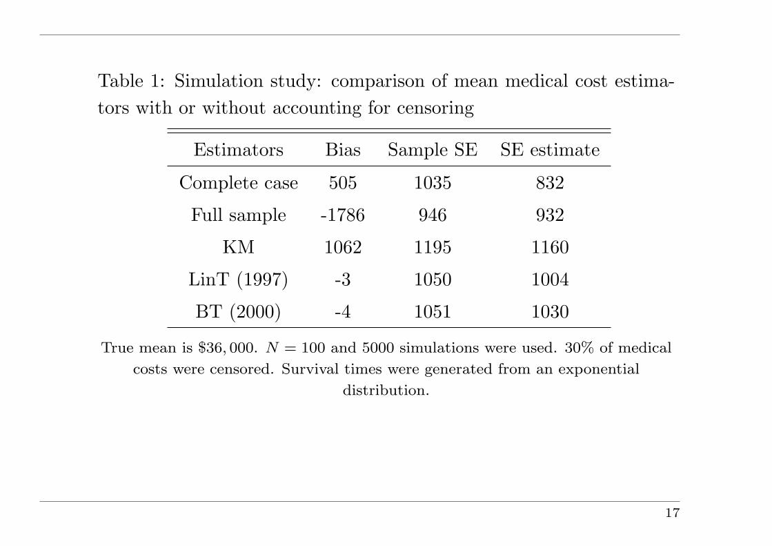
Table 1: Simulation study: comparison of mean medical cost estima-tors with or without accounting for censoring

Estimators Bias Sample SE SE estimate

Complete case 505 1035 832

Full sample -1786 946 932

KM 1062 1195 1160

LinT (1997) -3 1050 1004

BT (2000) -4 1051 1030

True mean is $36, 000. N = 100 and 5000 simulations were used. 30% of medical

costs were censored. Survival times were generated from an exponential

distribution.

17

Some efforts to simplify the estimators

1. Jiang and Zhou (2004) proposed a simpler formula for the originalBTp.

2. Pfeifer and Bang (2005) suggested a more user-friendlyrepresentation of the ZT estimator as

µZT =1n

n∑

i=1

[∆i

Mi

K(Ti)+ (1−∆i)

{Mi −M(Ci)}K(Ci)

]

where M(Ci) =∑n

j=1 I(Xj ≥ Ci)Mj(Ci)/∑n

j=1 I(Xj ≥ Ci), which isthe average of M ′s at Xi from i to n when the data {X, ∆,M} aresorted in ascending order based on X.This simplified formula clearly displays the contributions fromuncensored observations and censored observations to the estimator.

18

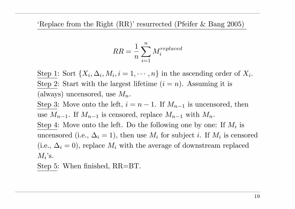
‘Replace from the Right (RR)’ resurrected (Pfeifer & Bang 2005)

RR =1n

n∑

i=1

Mreplacedi

Step 1: Sort {Xi,∆i,Mi, i = 1, · · · , n} in the ascending order of Xi.Step 2: Start with the largest lifetime (i = n). Assuming it is(always) uncensored, use Mn.Step 3: Move onto the left, i = n− 1. If Mn−1 is uncensored, thenuse Mn−1. If Mn−1 is censored, replace Mn−1 with Mn.Step 4: Move onto the left. Do the following one by one: If Mi isuncensored (i.e., ∆i = 1), then use Mi for subject i. If Mi is censored(i.e., ∆i = 0), replace Mi with the average of downstream replacedMi’s.Step 5: When finished, RR=BT.

19

Remarks:1. RR algorithm applied to {Xi, ∆i} = KM (Efron 1967)2. KM can be represented as IPW estimator (Satten and Datta2001).3. See Pfeifer & Bang (2005) or Example III later.4. This idea is intuitive and useful for point estimate but may not befor variance calculation.

20

Summary/overview

• These estimators can be classified into two classes:

– Approaches that only use complete final cost information,e.g., LinT, BT.

– Approaches that use additional information from cost historyfor both complete and censored individuals, e.g., LinA/B,BTp, ZT.

• We revealed how these estimators are analytically related andconditions under which estimators within each class becomeequivalent (see Appendix or Zhao, Bang, Wang & Pfeifer (2007)for proofs).

Remarks: 1. Other generalized frameworks: Robins et al. (1994),Cook & Lawless (1997), Huang & Louis (1998), Strawderman (2000).2. Efficiency theories are based on Robins et al. (1992, 1994, 1995).

21

Mean regression

1. Direct extension from Bang & Tsiatis (2000, 2002): To solve

1n

n∑

i=1

∆i

K(Ti)(Mi − β′Zi) = 0

2. Generalized linear models (Lin 2003):

E(Mki|Zki) = g(β′Zki)

where g is a specific link function (e.g., identity or exponential) andZki time-dependent covariates. This equation includes importantspecial cases of E(Mki|Zi) = β′kZi (Lin 2000a) andE(Mki|Zi) = µkexp(β′Zi).

22

3. Pattern-mixture models (Lin 2003):

E(Mki|Ti > ak;Zki) = g(β′Zki)

E(Mi|ak−1 < Ti ≤ ak;Zki) = g(β′Zki)

model conditional means of cost accumulation given specific survivalpatterns so the effects of differential survival times are removed.(Wait for an illustrative example why this is needed.)4. Proportional means regression (Lin 2000b):

E{Mi(t)|Zi} = µ0(t)exp(β′Zi)

where µ0(t) is an arbitrary positive function. — multiplicativecovariate effects5. Two-stage model (Carides et al. 2000)6. Flexible spline hazard model (Jain & Strawderman 2002) —modeling distribution as a function of covariates.7. Calibration regression (Huang 2002) –modeling cost and survivaltime together.

23

Median and its regression (Bang and Tsiatis 2002)

1n

n∑

i=1

∆i

K(Ti){I(Mi < median)− 1/2} ≈ 0 &

1n

n∑

i=1

∆i

K(Ti){I(Mi < β′Zi)− 1/2} ≈ 0

Remarks:1. A root of 1

n

∑ni=1{I(Mi < median)− 1/2} ≈ 0 is a minimizer of∑n

i=1 |Mi −median| for uncensored data (least absolute deviations).2. Discrete function of parameter so ≈ is needed.3. Grid search, simulated annealing or other alternatives can be usedfor parameter estimation.4. Computationally and numerically challenging— so not as popularas mean regression in practice.5. An efficient term can be added.

24

How about variance?

• All of the original papers present analytic variance formulae. Allbased on large sample theory.

• Pfeifer & Bang (2005) provide some user-friendly varianceformulae.

• Jiang and Zhou (2004) suggest a bootstrap-t confidence intervalto improve coverage (for skewed data).

25

Economic evaluation and CEA: a brief overview

• Definition of an economic evaluation: the comparative analysisof alternative courses of action in terms of both their costs andconsequences. Therefore, the basic tasks of any economicevaluation are to identify, measure, value and compare thecosts and consequences of the alternatives being considered.

• In CEA, we compare the difference in costs and difference inoutcomes between 2 interventions

• A standard measure: incremental cost-effectiveness ratio (ICER)

∆C

∆E=

µ1C − µ0C

µ1E − µ0E.

Let (C1, E1) and (C0, E0) denote the cost and effectivenessmeasures for a typical patient in the experimental and referentinterventions and have means (µ1C , µ1E) and (µ0C , µ0E).

26

• ICER, as a one-dimensional summary measure, can beinterpreted as the cost of obtaining an extra unit of effectiveness.

• Measures of effectiveness:

– Clinical and functional markers (e.g., life saved, life-yeargained, blood pressure, serum cholesterol, days withsymptoms, episodes, cases of disease)

– Quantitative gains in health

– Qualitative gains in health

• Mean cost can be used in the following health economics studies

– CEA: effectiveness is natural units such as survival time

– Cost-utility analysis: effectiveness is measured in terms ofyears of full health lived, such as quality-adjusted life years ordisability-adjusted life years (will be covered in the Part 2 ofthis course)

– Cost-benefit analysis: effectiveness is converted into monetaryunits.

27

• Some of statistical problems and solutions in ICER:

– Efficient estimation (Zhao & Tian 2001; Pullenayegum &Willan 2007)

– Covariate-adjustment (Gardiner 1999; Willan 2005)

– Various methods for CI for ratio statistic: Taylor’s, Fieller’s,Bootstrap, etc. Fan & Zhou (2007) compared 13 methods.

– Sample size and power (Gardiner et al. 2004)

• Other analytic measures/techniques: Cost-effectivenessacceptability curve, confidence ellipses, incremental net benefits,and willingness to pay, etc.– Suggested books are:Drummond et al. (2005). Methods for the Economic Evaluationof Health Care Programmes. Oxford Univ Press.Willan and Briggs (2006). The Statistical Analysis ofCost-effectiveness Data. Wiley & Sons.

28

Remarks:1. Widespread use of CEA and ICER. 43,895 and 27,200 articles bypubmed and Google scholar, respectively, for “cost-effectivenessanalysis”.2. More than 20 methodology papers on one statistical topic,“confidence interval of ICER”, have been published in peer-reviewedjournals. — this phenomenon is not so common in statistics!3. Unfortunately, issues in real world settings can be much morecomplicated than statistical issues.

29

Recent important papers on CEA in policy making1. Neumann. Why Don’t Americans Use Cost-EffectivenessAnalysis? Am J Manag Care 2004.

2. Neumann et al. (for the Panel on Integrating Cost-EffectivenessConsiderations into Health Policy Decisions) A Strategic Plan forIntegrating Cost-Effectiveness Analysis into the US HealthcareSystem. Am J Manag Care 2008.

3. American College of Physicians. Information onCost-Effectiveness: An Essential Product of a National ComparativeEffectiveness Program. Ann Intern Med 2008.With two editorials:– A Menu without Prices– Cost-Effectiveness Information: Yes, It’s Important, but Keep ItSeparate, Please!

30

Example I: Cost analysis using MADIT-II (Zhao etal. 2007; Zwanziger et al. 2006)

• The Multicenter Automatic Defibrillator Implantation Trial-II(MADIT-II)

• Randomized controlled trial which evaluated the effectiveness ofimplantable cardioverter defibrillator (ICD) vs. conventionaltherapy (Moss et al. 2002; Zwanziger et al. 2006)

• Dates and centers: 1997-2002 and 71 US, 5 Europe

• Eligibility Criteria:- Male/female age 21+ years with prior myocardial infarction- Ejection fraction ≤ 0.30- No electrophysiological testing requiredRemark: 32,000-60,000 people in the U.S. annually fit thesecriteria)

31

• Cost analysis was based on N = 664 (ICD, 17 crossovers) and431 (conventional, 23 crossovers).- To compare, N = 742 (ICD) and 490 (conventional) wereoriginally randomized.- For cost analysis, 109 European patients, 14 patients at 2 siteswith grossly incomplete cost data, and 14 patients withadditional missed cost data were excluded.

• Follow-up was between 11 and 55 months, averaging 22 months

• ICD demonstrated a longer survival with the estimated hazardratio of 0.69 (95% CI=0.51-0.93 with p=0.016).

• Due to high cost with the defibrillator and the implementationprocess, the CEA to evaluate the cost implication of the newtreatment was needed.

32

Remarks:1. In contrast, the MADIT-I randomized 196 patients who were athigh risk for ventricular arrhythmia to the same treatment options in1991-1996 (Moss et al. 1996; Mushlin et al. 1998)2. Both MADITs were supported by independent research grant fromGuidant, Inc.

33

Table 2: Medical cost estimates

Conventional therapy ICD

Estimators mean (SE) mean (SE)

Using 6-month intervals for boundaries

LinT 50,065 (5,497) 84,315 (4,921)

BT 49,796 (5,483) 84,353 (4,948)

LinA 39,578 (3,164) 77,539 (2,900)

LinB 47,855 (4,168) 84,315 (3,392)

BTp 46,803 (3,474) 83,887 (2,862)

ZT 44,666 (3,664) 83,629 (2,921)

Using distinct censoring times for boundaries

LinT=BT 49,796 (5,483) 84,353 (4,948)

LinA=LinB=BTp=ZT 44,666 (3,664) 83,629 (2,921)

34

Results

• LinA/B, Lin T and BTp estimates vary depending on theintervals we choose.

• With 6 month intervals, LinA is smaller than other estimates —shown to always underestimate the true mean.

• With the censoring times as partition boundaries, we haveLinT=BT and LinA/B=BTp=ZT.

• Since LinA/B, BTp and ZT utilize more information, they tendto be more efficient than LinT and BT that use only total costinformation.–Remark: Not theoretically guaranteed but generally true inmany practical situations. See the ZT and BT papers.

35

More analyses done

• ICER accounting for censoring and its confidence interval usingFieller’s method to account for covariance of costs and effects(Zhao & Tian 2001; Wang & Zhao 2006)– survival and costs discounted at 3% per year (expressed in 2001dollars)

• Projection to 12-year time horizon also attempted.

36

Example II: Regression using colorectal cancer datafrom Surveillance Epidemiology and End Results

(SEER) (Bang 2005)

• 71,519 colorectal cancer patients in SEER-Medicare database.

• Data {ID; gender; age at diagnosis; stage at diagnosis;month/year of diagnosis; month from diagnosis; month fromdeath, monthly sum of adjusted Medicare reimbursements} areretrieved.

• The entry was initiated at 1983, continued until 1993, and thedata collection concluded in 1994.

• For an illustrative purpose, a random sample of 2,000 patientswas selected.

• We analyzed T=min (death, 127 months).

37

Features/Complications with the SEER, a popular source of cost data (Lin 2003).

• Subjects may not survive beyond the time period of interest, andsurvival time is related to cost accumulation.

• Both survival time and cost accumulation process are subject toright censoring. Censoring was caused by the limited studyduration (so complete random censoring is likely). In otherstudies, loss to follow-up is also a major source of censoring.

• The cost data are normally recorded in broad time intervals, saymonthly or yearly intervals, and no information is available onhow the cost is accumulated within an interval. In SEER, thecost data were recorded in monthly intervals.

• The costs in different time intervals tend to be correlated.

38

Table 3: Baseline Characteristics

Covariates Whole samples (n = 71, 519) Subsamples (n = 2, 000)

male 52% 52%

age (in year) 76.6 (SD=7.14) 76.8 (SD=7.12)

stage 0 6.7% 6.9%

stage 1 22.6% 23.2%

stage 2 31.0% 31.1%

stage 3 22.5% 22.8%

stage 4 17.1% 16.1%

39

Table 4: Mean cost

Estimators Estimate

Complete case 41,581

Full sample 38,530

Mean (BT) 47,800

Median (BT) 34,000

40

Table 5: Median, mean, and lower (25%) and upper quartiles (75%)regression models on age and diagnostic stages

Parameters Lower Quartile Median Mean Upper Quartile

intercept 33,344 67,207 70,709 106,839

age -117 -546 -519 -861

stage 0 -2,590 2,718 4,550 3,697

stage 1 4,222 10,428 11,186 15,705

stage 2 7,767 12,640 15,831 21,614

stage 3 8,090 9,480 13,082 15,768

stage 4 reference

95% CIs are presented in Bang (2005).

41

Two additional scenarios were tried.

• Case 1 (original scenario): total cost upto death or 10 years

• Case 2: Total cost upto death or 3 years.

• Case 3: Same as Case 2 but we assumed death as censoringdefining full 3 year cost as the complete outcome.

42

Table 6: Median regression models in different scenarios

Parameters Case 1 (original) Case 2 Case 3

intercept 67,207 28,029 8,560

age -546 -40 280

stage 0 2,718 -9,796 -14,536

stage 1 10,428 -3,160 -9,796

stage 2 12,640 -284 -8,216

stage 3 9,480 6,004 -2,781

stage 4 reference

95% CIs are presented in Bang (2005).

43

Estimated Distribution Function of the Total Costs

wt, p and imp denote simple weighted, partitioned and improved estimators.

44

Results

• Age is negatively associated with total cost.

• Stage 2 incurred the largest cost. Why?— Higher costs may reflect the deleterious effect of more seriousdisease or the beneficial effect of living longer! So cautiousinterpretations are needed.— ‘Conditional’ methods controlling survival time may be bettersuited (Lin 2003).

• As anticipated, the mean cost lies between the median and theupper quartile.

• Cost and predictors can be highly different for long vs.short-term costs.

• Separate estimation of initial vs. continuing vs. final costs maybe informative (Yabroff et al. 2008).

45

Example III: Estimation of customer lifetime value(Pfeifer & Bang 2005)

• In marketing, customer lifetime value (CLV), lifetime customervalue, or lifetime value and a new concept of “customer life cyclemanagement” is the present value of the future cash flowsattributed to the customer relationship. Use of CLV as amarketing metric tends to place greater emphasis on customerservice and long-term customer satisfaction, rather than onmaximizing short-term sales.

• How to use data from a random sample of customer relationshipsto calculate an appropriate average CLV.

• A mix of active and completed relationships — censoring.

46

• Weighted Complete Cases (WCC) or Replace from the Right(RR): Replace each censored CLV with average downstreamreplaced CLVs and then average. This is identical to BTestimator.

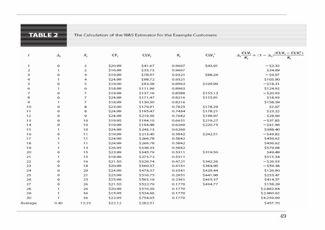
• Weighted Available Sample (WAS): Adjusts based on comparingCLV to date of censored cases to the average CLV at that date ofall cases. This is ZT estimator.

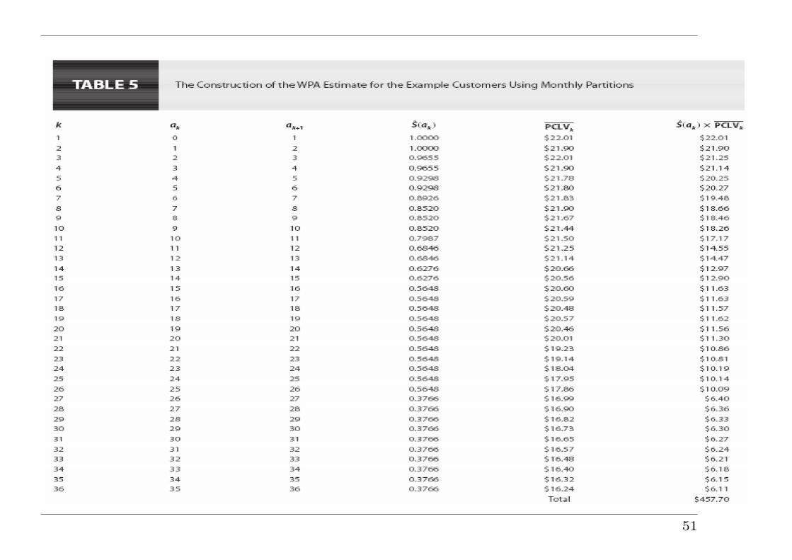
• Weighted Partition Average (WPA): Combines average partitionCLVs using KM survival probabilities. This is Lin’s estimator.

47

48

49

50

51

Statistical research on cost (and CEA) for the last 10 years

• Consistent and efficient estimators

• Analytic formulae and bootstrapping for variance

• Mean and median/quantile regression

• Classical or unified framework. Search for more practicalestimators and relationships among estimators

• Mostly non- or semi-parametric but some parametric approachesavailable: Random effects models

• Longitudinal data

• Multi-parts model

• Dynamic Markov model, Bayesian methods, Decision trees, etc.

52

Other issues

• Discounting can be important in any cost analysis- The present value of an expenditure of M dollars in t years inthe future with an interest rate of r is:

Mpresent =Mfuture

(1 + r)t

where the recommended real discount rate for CEA is 3%. Forsensitivity analyses, 0− 7% is used.

• Left censoring: limited attention and research

• Tail problem or small denominator problem in weighting mayoccur. Bang (2005) and Hothorn et al. (2006) suggested someremedies and Robins and Wang (2000) and Robins et al. (2008)discussed this issue in detail.

53

Conclusions and Discussions

• Standard statistical methods for survival data should NOT be used for

medical cost data - Proved 10 years ago. Time to stop.

• Question/observations for many years: Several estimators have been

developed from different theoretical backgrounds. They behave

similarly. Why? Now we know.

• Different estimators are needed for different data availabilities.

• Relationships among estimators may have limited impacts on

applications but are mathematically/theoretically important!

• When you think that you invented a new thing, you should check if

this is really new or at least if there are some advantages in it (e.g.,

offer easy variance estimation, or more intuitive or user-friendly

formula).

• Limitation: No standard software yet. Should consult with

experienced statisticians in this field.

54

Relevant publications by instructors

• Bang H, Tsiatis AA. (2000). Estimating medical costs withcensored data. Biometrika 87: 329-343.

• Zhao H, Tian L. (2001). On Estimating medical cost andincremental cost-effectiveness ratios With censored data.Biometrics 57:1002-1008.

• Bang H, Tsiatis AA. (2002). Median regression with censoredcost data. Biometrics 58: 643-649.

• Bang H. (2005). Medical cost analysis: an application tocolorectal cancer data from the SEER Medicare database. ContClin Trials 26: 586-597.

• Pfeifer PE, Bang H. (2005). Non-parametric estimation of meancustomer lifetime value. J of Int Marketing 19:48-66.

• Zwanziger J, Hall WJ, Dick AW, Zhao H, et al. (2006). The cost55

effectiveness of implantable cardioverter-defibrillators: resultsfrom the multicenter automatic defibrillator implantation trial(MADIT)-II. Am Col Cardiol 47:2310-2318.

• Wang H, Zhao H. (2006). Estimating incrementalcost-effectiveness ratios and their confidence intervals withdifferentially censored data. Biometrics 62:570-575.

• Zhao H, Bang H, Wang H, Pfeifer PE. (2007). On theequivalence of some medical cost estimators with censored data.Stat Med 26:4520-4530.

56

Appendix: Equivalences amongestimators (Zhao, Bang, Wang &

Pfeifer 2007)

Prior efforts on showing equivalences

• Bang and Tsiatis (2000) showed BT=Huang & Louis analytically.

• Strawderman (2000) showed Cook & Lawless (suited forrecurrent event processes subject to dependent termination) is acontinuous analog of Lin.

• O’Hagan and Stevens (2004) showed BT=LinT via infinitesimalpartitions.

• Pfeifer and Bang (2005) showed RR=BT (sketchy proof) andnoted ZT=LinA/B numerically in some simulations.

57

New equivalences revealed

• Additional notations

– Subintervals are formed by J distinct censoring times,tC1 , · · · , tCJ in the manner that non-overlapping J + 1subintervals, (0 = tC0 , tC1 ], (tC1 , tC2 ], · · · , (tCJ , tCJ+1 = τ ],encompass the entire time (0, τ ].

– Suppose the number of subjects who get censored at time tCjis nC

j (j = 1, · · · , J).

– The number of subjects who die during (tCj−1, tCj ] interval is

ndj (j = 1, · · · , J + 1).

– If a subject dies exactly at the censoring time, say tCj , weassume that the time of event happened slightly earlier thanthe censoring time so it belongs to the interval (tCj−1, t

Cj ].

58

• The KM estimates for the survival distribution of the censoringtime at each of these partition points are denoted as K1, · · · , KJ .At the beginning, K0 = 1. Since K(t) takes jumps only at timetCj for j = 1, · · · , J , we have

K(Ti) = Kj−1 for tCj−1 < Ti ≤ tCj .

• The KM estimates for the survival distribution of the failure timeat each of these partition points are denoted as S1, · · · , SJ withS0 = 1 and SJ+1 = 0.

• Define Yj =∑n

i=1 I(Xi > tCj ), i.e., the number of subjects whosurvive without being censored at time tCj and let∆ij = I(tCj−1 < Xi ≤ tCj , ∆i = 1) be the indicator for subject i

who fails within (tCj−1, tCj ], and ∆C

ij = I(Xi = tCj , ∆i = 0) be theindicator for subject i who is censored at time tCj .

59

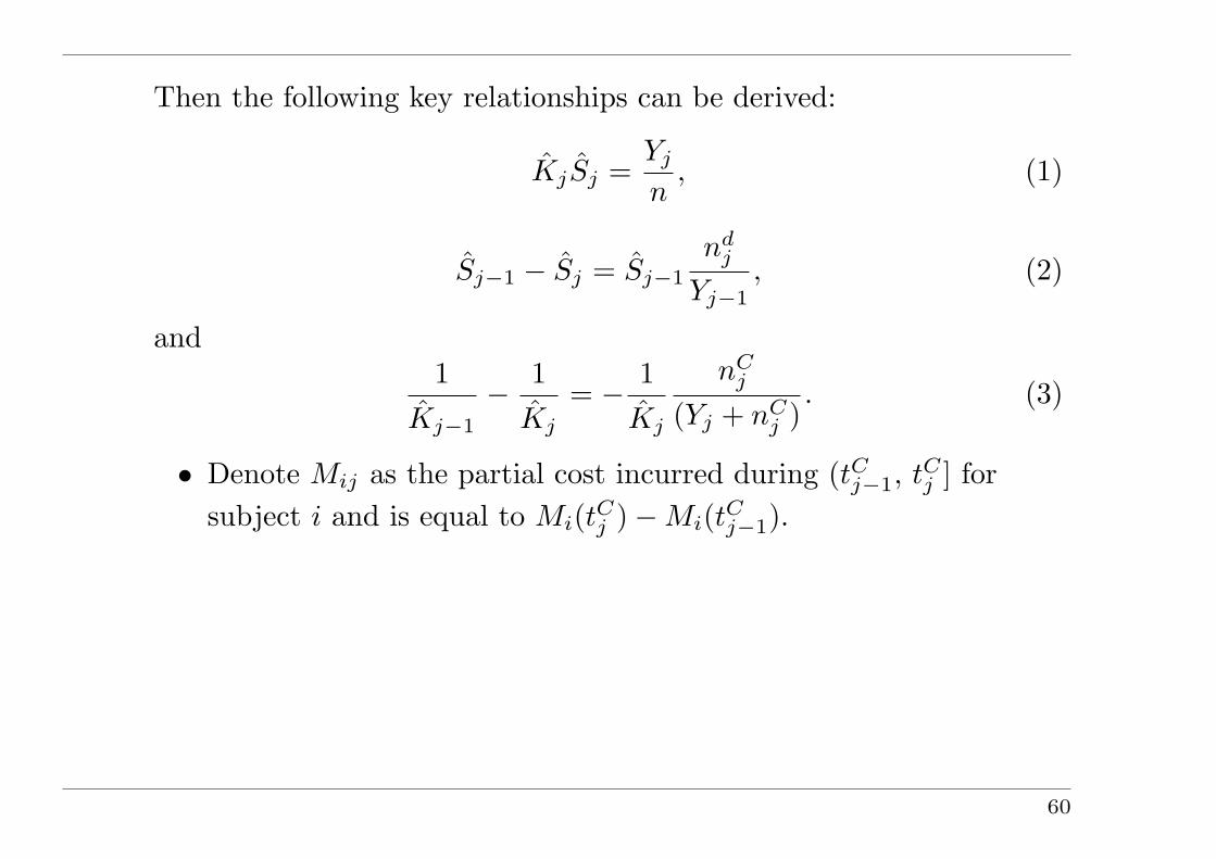
Then the following key relationships can be derived:

KjSj =Yj

n, (1)

Sj−1 − Sj = Sj−1

ndj

Yj−1, (2)

and1

Kj−1

− 1Kj

= − 1Kj

nCj

(Yj + nCj )

. (3)

• Denote Mij as the partial cost incurred during (tCj−1, tCj ] forsubject i and is equal to Mi(tCj )−Mi(tCj−1).

60

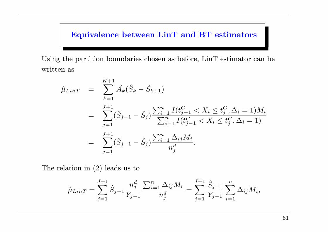
Equivalence between LinT and BT estimators

Using the partition boundaries chosen as before, LinT estimator can be

written as

µLinT =

K+1∑

k=1

Ak(Sk − Sk+1)

=

J+1∑j=1

(Sj−1 − Sj)

∑ni=1 I(tC

j−1 < Xi ≤ tCj , ∆i = 1)Mi∑n

i=1 I(tCj−1 < Xi ≤ tC

j , ∆i = 1)

=

J+1∑j=1

(Sj−1 − Sj)

∑ni=1 ∆ijMi

ndj

.

The relation in (2) leads us to

µLinT =

J+1∑j=1

Sj−1nd

j

Yj−1

∑ni=1 ∆ijMi

ndj

=

J+1∑j=1

Sj−1

Yj−1

n∑i=1

∆ijMi,

61

and, further by (1),

µLinT =

J+1∑j=1

1

n

n∑i=1

∆ijMi

Kj−1

=

J+1∑j=1

1

n

n∑i=1

∆ijMi

K(Ti)=

1

n

n∑i=1

∆iMi

K(Ti)= µBT .

62

Equivalence between ZT and LinA/B Estimators

LinA/B can be written as

µLinA/B =J+1∑

j=1

Sj−1

∑ni=1 I(Xi > tCj−1)Mij∑n

i=1 I(Xi > tCj−1)=

J+1∑

j=1

Sj−1

Yj−1

n∑

i=1

I(Xi > tCj−1)Mij .

(4)For j = 1 term in the summation over j in (4), since S0 = 1, Y0 = n

and K(Ti) = 1 for Ti < tC1 , we can rewrite this term as

1n

{n∑

i=1

∆i1Mi

K(Ti)+

n∑

i=1

∆Ci1Mi +

n∑

i=1

I(Xi > tC1 )Mi(tC1 )

}(5)

where three sums in (5) represent contributions from those who trulyfailed within the first interval, those who were permanently censoredwithin the same interval, and those who are yet to fail at the end ofthis interval, respectively.

63

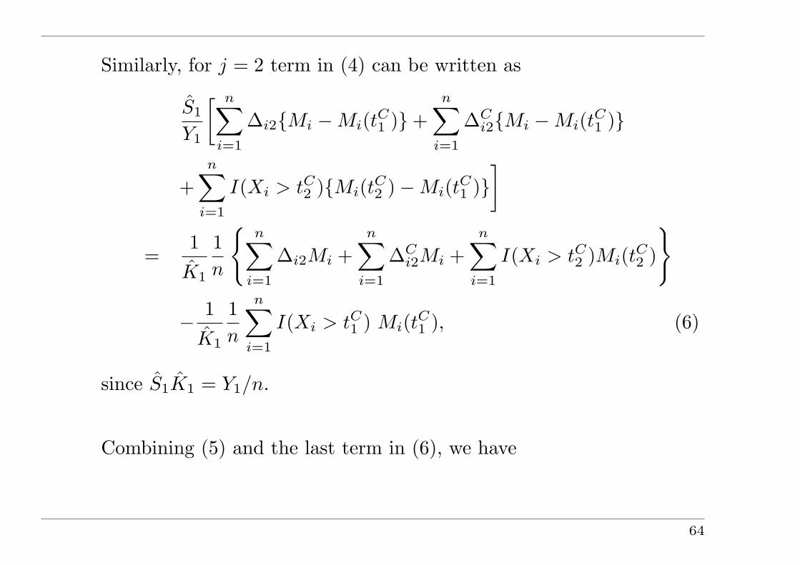
Similarly, for j = 2 term in (4) can be written as

S1

Y1

[ n∑

i=1

∆i2{Mi −Mi(tC1 )}+n∑

i=1

∆Ci2{Mi −Mi(tC1 )}

+n∑

i=1

I(Xi > tC2 ){Mi(tC2 )−Mi(tC1 )}]

=1

K1

1n

{n∑

i=1

∆i2Mi +n∑

i=1

∆Ci2Mi +

n∑

i=1

I(Xi > tC2 )Mi(tC2 )

}

− 1K1

1n

n∑

i=1

I(Xi > tC1 ) Mi(tC1 ), (6)

since S1K1 = Y1/n.

Combining (5) and the last term in (6), we have

64

1

n

{n∑

i=1

∆i1Mi

K(Ti)+

n∑i=1

∆Ci1Mi +

(1− 1

K1

) n∑i=1

I(Xi > tC1 )Mi(t

C1 )

}

=1

n

{n∑

i=1

∆i1Mi

K(Ti)+

1

K1

n∑i=1

∆Ci1Mi +

(1

K0

− 1

K1

) n∑i=1

I(Xi ≥ tC1 )Mi(t

C1 )

}

=1

n

[n∑

i=1

∆i1Mi

K(Ti)+

1

K1

{n∑

i=1

∆Ci1Mi − nC

1

(Y1 + nC1 )

n∑i=1

I(Xi ≥ tC1 )Mi(t

C1 )

}]

=1

n

[n∑

i=1

∆i1Mi

K(Ti)+

n∑i=1

∆Ci1{Mi −M(tC

1 )}K1

].

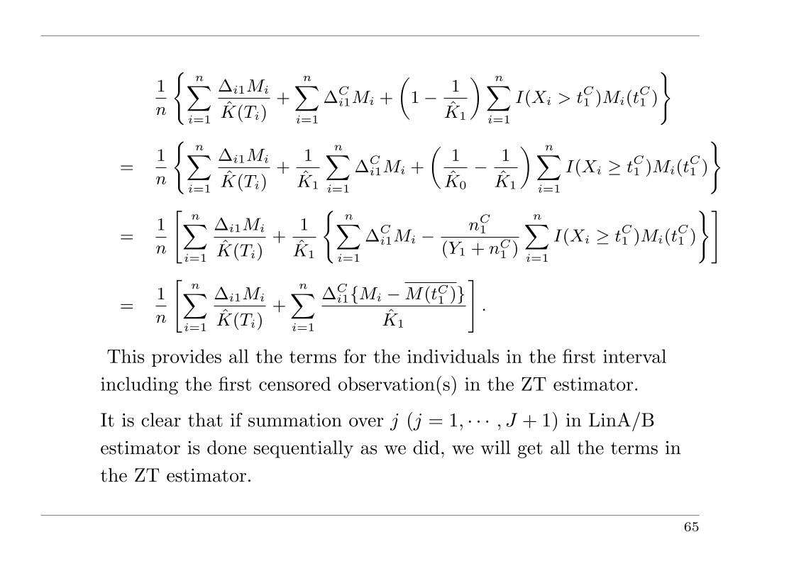
This provides all the terms for the individuals in the first intervalincluding the first censored observation(s) in the ZT estimator.

It is clear that if summation over j (j = 1, · · · , J + 1) in LinA/Bestimator is done sequentially as we did, we will get all the terms inthe ZT estimator.

65

Equivalence between BTp and LinA/B Estimators

In a general partition with (ak, ak+1], k = 1, · · · ,K, and a1 = 0,aK+1 = τ , the partitioned estimator BTp is not efficient, since foreach censored observation, say at time Ci, the cost informationbetween the time maxak≤Ciak and Ci is not utilized.

However, using the partition boundaries at the distinct censoringtimes tC1 , · · · , tCJ following the same logic we used previously, BTpestimator in the jth interval can be written as

1n

n∑

i=1

∆jiMij

K(T ji )

.

This includes subjects who die inside the jth interval (tCj−1, tCj ] and

also those subjects whose Xi’s are greater than or equal to tCj . Thesesubjects with Xi ≥ tCj are considered complete observation by the

66

definition of ∆ji . They are equivalent to being dead at time tCj for the

purpose of cost estimation within this interval.

Hence, their K(Ti) = Kj−1 because we assume that death alwayshappens a little bit earlier than the actual time of censoring if theyoccur simultaneously. So the above term can be rewritten as

1n

1Kj−1

n∑

i=1

I(Xi > tCj−1)Mij =Sj−1

Yj−1

n∑

i=1

I(Xi > tCj−1)Mij ,

which is exactly the same as the jth term of LinA/B.Therefore, we conclude that LinA/B, BTp (and ZT) estimators areall equivalent with the partitions formed at the distinct censoringtimes.

67