Embed Size (px)
Citation preview

University of Southern Queensland
Faculty of Health, Engineering & Sciences
Analysis of bridges subjected to
flood loadings based on different
design standards
A dissertation submitted by
Bradley Jordan
In fulfilment of the requirements of
Course ENG4112 – Research Project
Towards the degree of
Bachelor of Engineering (Honours) (Civil)
Submitted: October, 2015

i
ABSTRACT
The need to design bridges to withstand flood and debris loads has long been recognised
in Australia, however bridges are still failing to live their entire design life when subjected
to extreme flooding events. This research project presents a structural evaluation of
bridges when subjected to the current flood loadings from design standards around the
world. A case study bridge has been selected to apply the flood loads on. The case study
bridge chosen is Tenthill Creek Bridge, located within the Lockyer Valley Region.
The flood loadings that were identified from the design standards were drag, lift and
debris forces as well as log-impact loads. Static components that were also included in
the model were hydrostatic pressure as well as buoyancy. The structural components of
the bridge that were identified to be analysed were the piers and superstructures. The
structural evaluation has been performed using a finite element analysis (FEA) software
package, Strand7. The model was analysed by Strand7’s linear static analysis.
Displacement and stress concentration results were then produced and analysed. The
results indicate that the Australian Standards produced, on average, 20% more adverse
effects in comparison to the international standards. The results indicate that no
recommendations could be made for the Australian Standards, based on the results
produced by the International Standards. Further work will need to be conducted if
specific recommendations are to be made for the Australian Standards.

ii
University of Southern Queensland
Faculty of Health, Engineering and Sciences
ENG4111/ENG4112 Research Project
LIMITATIONS OF USE
The Council of the University of Southern Queensland, its Faculty of Health, Engineering
& Sciences, and the staff of the University of Southern Queensland, do not accept any
responsibility for the truth, accuracy or completeness of material contained within or
associated with this dissertation.
Persons using all or any part of this material do so at their own risk, and not at the risk of
the Council of the University of Southern Queensland, its Faculty of Health, Engineering
& Sciences or the staff of the University of Southern Queensland.
This dissertation reports an educational exercise and has no purpose or validity beyond
this exercise. The sole purpose of the course pair entitled “Research Project” is to
contribute to the overall education within the student’s chosen degree program. This
document, the associated hardware, software, drawings, and other material set out in the
associated appendices should not be used for any other purpose: if they are so used, it is
entirely at the risk of the user.
Dean
Faculty of Health, Engineering & Sciences

iii
CERTIFICATION OF DISSERTATION
I certify that the ideas, designs and experimental work, results, analyses and conclusions
set out in this dissertation are entirely my own effort, except where otherwise indicated
and acknowledged.
I further certify that the work is original and has not been previously submitted for
assessment in any other course or institution, except where specifically stated.
Full name: Bradley Jordan
Student Number: 0061033342

iv
ACKNOWLEDGMENTS
I would like to acknowledge my supervisors Weena Lokuge and Karu Karunasena, as
well as Buddhi Wahalathrantri, for their constant guidance and support throughout this
project. This project would not be possible without their guidance and support.

v
TABLE OF CONTENTS
Abstract ............................................................................................................................. 1
Limitations of Use ............................................................................................................. 2
Certification of Dissertation .............................................................................................. 3
Acknowledgments ............................................................................................................. 4
List of Figures ................................................................................................................. 12
List of Tables................................................................................................................... 15
List of Appendices .......................................................................................................... 17
Chapter 1 Introduction ................................................................................................. 1
1.1 Chapter overview .............................................................................................. 1
1.2 Background ....................................................................................................... 1
1.3 Project aim ........................................................................................................ 2
1.4 Method of investigation .................................................................................... 2
1.5 Project Objectives ............................................................................................. 3
1.6 Structure of this thesis ....................................................................................... 3
Chapter 2 Literature Review ........................................................................................ 6
2.1 Chapter overview .............................................................................................. 6
2.2 Bridges around the world .................................................................................. 6
2.2.1 Concrete ...................................................................................................... 6
2.2.1.1 Reinforced Concrete ............................................................................ 6
2.2.1.2 Prestressed Concrete ............................................................................ 7
2.2.2 Steel ........................................................................................................... 10
2.2.3 Timber ....................................................................................................... 11
2.3 Concrete Bridges ............................................................................................. 13
2.3.1 General terminology.................................................................................. 13
2.3.2 Construction methods used ....................................................................... 14
2.3.2.1 Falsework/staging .............................................................................. 15

vi
2.3.2.2 Incremental Launching ...................................................................... 15
2.3.2.3 Span-by-span ..................................................................................... 16
2.3.2.4 Balanced cantilever ............................................................................ 17
2.3.3 Types of bridges ........................................................................................ 17
2.3.3.1 Arch bridges ....................................................................................... 18
2.3.3.2 Reinforced slab bridges ..................................................................... 18
2.3.3.3 Beam and slab bridges ....................................................................... 19
2.3.3.4 Box girder bridges ............................................................................. 20
2.3.3.5 Integral bridges .................................................................................. 20
2.3.3.6 Cable-stayed bridges .......................................................................... 21
2.3.3.7 Suspension bridges ............................................................................ 21
2.3.4 Design life ................................................................................................. 22
2.3.5 Modes of failure ........................................................................................ 22
2.3.5.1 Mechanical failure ............................................................................. 23
2.3.5.2 Scouring ............................................................................................. 23
2.3.5.3 Deterioration/spalling ........................................................................ 23
2.3.6 How they are maintained .......................................................................... 24
2.2.3.1 Preventative maintenance .................................................................. 25
2.2.3.2 Rehabilitation ..................................................................................... 25
2.4 Natural Disasters ............................................................................................. 26
2.4.1 Flooding .................................................................................................... 26
2.4.1.1 Slow-onset flooding ........................................................................... 26
2.4.1.2 Rapid-onset flooding.......................................................................... 26
2.4.1.3 Flash flooding .................................................................................... 27
2.4.1.4 Bridge failures due to flooding .......................................................... 27
2.4.2 Earthquake................................................................................................. 28
2.4.3 Cyclone ..................................................................................................... 29

vii
2.4.4 Bushfire ..................................................................................................... 30
2.5 Extreme flood events in Australia ................................................................... 33
2.5.1 Summer 2010/2011 Queensland flood events........................................... 33
2.5.2 2013 Queensland flood events (Cyclone Oswald) .................................... 34
2.6 Forces exhibited during a flooding event ........................................................ 37
2.6.1 Hydrostatic pressure .................................................................................. 37
2.6.2 Buoyancy .................................................................................................. 38
2.6.3 Impact force .............................................................................................. 39
2.6.4 Drag force.................................................................................................. 39
Chapter 3 Australian Bridge design standards ........................................................... 41
3.1 Chapter overview ............................................................................................ 41
3.2 Introduction ..................................................................................................... 41
3.3 Fluid forces on piers ........................................................................................ 41
3.3.1 Drag force.................................................................................................. 42
3.3.2 Lift forces .................................................................................................. 43
3.3.3 Debris forces ............................................................................................. 43
3.4 Fluid forces on superstructures ....................................................................... 44
3.4.1 Drag force.................................................................................................. 44
3.4.2 Lift force.................................................................................................... 45
3.5 Debris forces ................................................................................................... 46
3.6 Effects due to logs ........................................................................................... 47
3.7 Effects due to buoyancy .................................................................................. 48
3.8 Effects due to debris ........................................................................................ 48
3.8.1 Depth of debris mat ................................................................................... 49
3.8.2 Debris acting on piers................................................................................ 49
3.8.3 Debris acting on superstructures ............................................................... 49
3.9 Traffic loads .................................................................................................... 49

viii
3.10 Load combinations .......................................................................................... 52
Chapter 4 International Bridge Design Standards ..................................................... 54
4.1 Chapter overview ............................................................................................ 54
4.2 European Bridge Design Standards (Ba 59/94) .............................................. 54
4.2.1 Hydrodynamic forces on piers .................................................................. 54
4.2.1.1 Flow pressure ..................................................................................... 54
4.2.1.2 Drag force .......................................................................................... 55
4.2.1.3 Lift force ............................................................................................ 56
4.2.2 Hydrodynamic forces on submerged bridge superstructures .................... 56
4.2.2.1 Drag force .......................................................................................... 56
4.2.3 Debris forces ............................................................................................. 56
4.2.3.1 Impact loads due to logs .................................................................... 56
4.2.4 Debris restricting the flow ......................................................................... 57
4.2.5 Load combinations and load factors ......................................................... 57
4.3 American Bridge Design Standards (AASHTO, 2012) .................................. 59
4.3.1 Static Pressure ........................................................................................... 59
4.3.2 Buoyancy .................................................................................................. 59
4.3.3 Stream Pressure ......................................................................................... 59
4.3.3.1 Longitudinal (drag) ............................................................................ 59
4.3.3.2 Lateral (lift) ........................................................................................ 60
4.3.4 Effects due to debris .................................................................................. 61
4.3.5 Load combinations .................................................................................... 61
4.4 Asian Bridge Design Standards (Indian code of practice) .............................. 64
4.4.1 Pier forces due to water currents ............................................................... 64
4.4.1.1 Water flowing parallel to the direction of the pier............................. 64
4.4.1.2 Water flowing at an angle to the pier ................................................. 66
4.4.2 Buoyancy .................................................................................................. 67

ix
4.4.3 Load combinations .................................................................................... 68
Chapter 5 Project Planning – Methodology ............................................................... 69
5.1 Chapter overview ............................................................................................ 69
5.2 Methodology outline ....................................................................................... 69
5.3 Identification of a Complex Bridge ................................................................ 70
5.3.1 Location of the bridge ............................................................................... 70
5.3.2 Bridge details ............................................................................................ 71
5.3.3 Geometry of the structure.......................................................................... 72
5.3.4 Ground profile ........................................................................................... 74
5.3.5 Parameters required ................................................................................... 75
3.5.4 Assumptions ................................................................................................... 78
5.4 Simulation Method .......................................................................................... 80
Chapter 6 Simulation ................................................................................................. 81
6.1 Chapter Overview ........................................................................................... 81
6.2 Simple bridge deck model ............................................................................... 81
6.2.1 Model development ................................................................................... 81
6.2.2 Simulation parameters ............................................................................... 81
6.2.3 Input parameters ........................................................................................ 84
6.2.4 Simulation results ...................................................................................... 85
6.2.5 Discussion ................................................................................................. 86
6.3 Tenthill Creek Bridge ...................................................................................... 88
6.3.1 Creating the geometric model ................................................................... 88
6.3.2 Material properties .................................................................................... 89
6.3.3 Restraints of the model.............................................................................. 89
6.3.4 Meshing of the model................................................................................ 90
Chapter 7 Results and Discussion .............................................................................. 94
7.1 Chapter overview ............................................................................................ 94

x
7.2 AS5100 ............................................................................................................ 94
7.2.1 Load cases and load combinations ............................................................ 94
7.2.2 Simulation results ...................................................................................... 98
7.3 International Design Standards ..................................................................... 105
7.3.1 BA 59/94 ................................................................................................. 105
7.3.1.1 Load cases and load combinations................................................... 105
7.3.1.2 Simulation results ............................................................................ 106
7.3.2 AASHTO ................................................................................................ 107
7.3.2.1 Load cases and load combinations................................................... 107
7.3.2.2 Simulation results ............................................................................ 108
7.3.3 Indian code of practice ............................................................................ 108
7.3.3.1 Load cases and load combinations................................................... 108
7.3.3.2 Simulation results ............................................................................ 109
7.4 Comparison of the standards ......................................................................... 110
Chapter 8 Conclusions and Futher Work ................................................................. 114
8.1 Summary ....................................................................................................... 114
8.2 Achievement of Project Objectives ............................................................... 114
8.3 Conclusions ................................................................................................... 116
8.4 Recommendations for future work................................................................ 117
8.4.1 Incorporation of steel reinforcement ....................................................... 117
8.4.2 Accurate modelling of the flow behaviour ............................................. 117
References ..................................................................................................................... 121
Appendices .................................................................................................................... 126
Appendix A – Project Specifications ........................................................................ 126
Appendix B – Flood frequency analysis data for Tenthill Creek.............................. 127
Appendix C – Detailed calculations .......................................................................... 131
Parametric study calculations ................................................................................ 131

xi
AS5100 load calculations ...................................................................................... 134
BA59/94 load calculations .................................................................................... 151
AASHTO load calculations................................................................................... 152
Indian Code of Practice calculations ..................................................................... 153
Appendix D – Flood load values ............................................................................... 154
AS5100 flood loads ............................................................................................... 154
BA59/94 flood loads ............................................................................................. 159
AASHTO .............................................................................................................. 160
Indian Code of Practice ......................................................................................... 161
Appendix E – Tenthill bridge Strand7 model results figures .................................... 162
AS5100 results ...................................................................................................... 162
BA 59/94 results .................................................................................................... 165
AASHTO results ................................................................................................... 166
Indian Code of Practice Results: ........................................................................... 167
Appendix F – Resource Requirements ...................................................................... 169
Appendix G – Risk Assessment ................................................................................ 170

xii
LIST OF FIGURES
Figure 1.1 - Lockyer Valley location ................................................................................ 1
Figure 2.1 - Reinforced concrete slabs .............................................................................. 7
Figure 2.2 - Prestressed concrete girder box ..................................................................... 8
Figure 2.3 - Pre-tensioned concrete .................................................................................. 9
Figure 2.4 - Post-tensioned concrete ............................................................................... 10
Figure 2.5 - A typical steel truss bridge .......................................................................... 11
Figure 2.6 - A typical timber truss bridge ....................................................................... 12
Figure 2.7 - Typical components of a bridge .................................................................. 14
Figure 2.8 - Falsework used for a long spanning concrete bridge .................................. 15
Figure 2.9 - Incremental launching of a bridge ............................................................... 16
Figure 2.10 - Span-by-span construction of a bridge ...................................................... 17
Figure 2.11 – Long-span arch bridge .............................................................................. 18
Figure 2.12 - Reinforced slab bridge .............................................................................. 19
Figure 2.13 - Beam and slab bridge in construction ....................................................... 19
Figure 2.14 - Box girder bridge in construction .............................................................. 20
Figure 2.15 - Dee River Crossing cable-stayed bridge ................................................... 21
Figure 2.16 - Suspension bridge...................................................................................... 22
Figure 2.17 - Scouring around a bridge foundation ........................................................ 23
Figure 2.18 - Deterioration of an overpass ..................................................................... 24
Figure 2.19 - Bridge collapse cause by Cumbria floods ................................................. 27
Figure 2.20 - Complete collapse of a bridge in Santiago due to an earthquake .............. 28
Figure 2.21 - A blown away bridge cause by Cyclone Hudhud ..................................... 30
Figure 2.22 - Destruction of the Feng Yu Bridge in China ............................................. 32
Figure 2.23 - Urban debris being thrown into a bridge ................................................... 34
Figure 2.24 - Scoured road approach at bridge abutment ............................................... 34
Figure 2.25 - Silt deposition on Liftin Bridge approach ................................................. 35
Figure 2.26 – Damage to the Murphy Bridge ................................................................. 36
Figure 2.27 - Damage to the Willows Bridge ................................................................. 36
Figure 2.28 - Pressure prism of a submerged object ....................................................... 37
Figure 2.29 - A floating object ........................................................................................ 38
Figure 2.30 - A sinking object......................................................................................... 38

xiii
Figure 2.31 - A neutrally buoyant object ........................................................................ 38
Figure 3.1 - Drag and lift forces on piers ........................................................................ 42
Figure 3.2 - Pier debris Cd ............................................................................................... 44
Figure 3.3 - Superstructure Cd ......................................................................................... 44
Figure 3.4 - Dimensions required.................................................................................... 45
Figure 3.5 - Superstructure CL ........................................................................................ 46
Figure 3.6 - Superstructure debris Cd .............................................................................. 47
Figure 3.7 - M1600 moving traffic loads ........................................................................ 50
Figure 3.8 - Ultimate flood load factor ........................................................................... 53
Figure 4.1 - Load combination factors ............................................................................ 58
Figure 4.2 – Plan view of pier showing stream flow pressure ........................................ 60
Figure 4.3 - Debris mat ................................................................................................... 61
Figure 4.4 - Velocity diagram ......................................................................................... 64
Figure 4.5 - Classification of different shaped bridge piers ............................................ 65
Figure 5.1 - Location of Tenthill Creek Bridge .............................................................. 70
Figure 5.2 - Tenthill Creek Bridge .................................................................................. 71
Figure 5.3 - Cross-sectional view ................................................................................... 71
Figure 5.4 - Cross-sectional view ................................................................................... 72
Figure 5.5 - Front and side views of the piers ................................................................. 73
Figure 5.6 Girder dimensions ......................................................................................... 73
Figure 5.7 - Side view of the bridge ................................................................................ 74
Figure 5.8 - Ground profile provided by the Queensland Department of Transport and
Main Roads ..................................................................................................................... 74
Figure 5.9 - Simplified ground profile with appropriate conversions ............................. 75
Figure 5.10 - Upstream view of the gauge station .......................................................... 77
Figure 5.11 - Annual flood frequency analysis for Tenthill Creek ................................. 77
Figure 6.1 - Cross sectional view of the structure ........................................................... 81
Figure 6.2 - Typical pin and roller support ..................................................................... 83
Figure 6.3 - Coarse simulation model ............................................................................. 83
Figure 6.4 - Medium simulation model .......................................................................... 84
Figure 6.5 - Fine simulation model ................................................................................. 84
Figure 6.6 - Deformed model set a 5% displacement scale ............................................ 86
Figure 6.7 - Final geometric model ................................................................................. 88

xiv
Figure 6.8 - Degrees of freedom for fixed (left), pinned (middle) and roller (right) links
......................................................................................................................................... 90
Figure 6.9 - Deck sections ............................................................................................... 92
Figure 6.10 – Girder (left) and pier (right) sections ........................................................ 92
Figure 6.11 - Headstock sections .................................................................................... 92
Figure 6.12 - Meshed model ........................................................................................... 93
Figure 7.1 - Bar chart of X, Y and Z displacement results ............................................. 98
Figure 7.2 - X-displacement contour plot ....................................................................... 99
Figure 7.3 - Location of maximum X-displacement in the positive X-direction ............ 99
Figure 7.4 - Location of maximum X-displacement in the negative X-direction ......... 100
Figure 7.5 - Y-displacement contour plot ..................................................................... 100
Figure 7.6 - Location of maximum Y-displacement ..................................................... 101
Figure 7.7 - Z-displacement of the AS5100 model ....................................................... 101
Figure 7.8 - Location of maximum Z-displacement ..................................................... 102
Figure 7.9 - Bar chart of X, Y and Z stress concentrations ........................................... 103
Figure 7.10 - Bar chart of XYZ stress and displacement results .................................. 104
Figure 7.11 - Bar chart stress and displacement results ................................................ 110
Figure 7.12 - Bar chart comparing displacement results............................................... 111
Figure 7.13 - Bar chart of X, Y and Z stress concentration results ............................... 112
Figure 8.1 - Sluice gate type of pressure flow .............................................................. 118
Figure 8.2 - Fully submerged pressure flow ................................................................. 118
Figure 8.3 - Pressure and weir flow behaviour ............................................................. 119
xv
LIST OF TABLES
Table 2.1 - Cyclone categories ........................................................................................ 29
Table 2.2 - Queensland fire danger categories ................................................................ 31
Table 3.1 - Load factors for dead loads........................................................................... 48
Table 3.2 - Lane load factors........................................................................................... 50
Table 3.3 - Dynamic load allowance............................................................................... 51
Table 3.4 - Traffic load factors ....................................................................................... 51
Table 3.5 - Dead load factors .......................................................................................... 52
Table 3.6 - Ultimate load factors..................................................................................... 53
Table 4.1 - K values ........................................................................................................ 55
Table 4.2 – Drag Coefficients ......................................................................................... 60
Table 4.3 - Lift coefficient .............................................................................................. 61
Table 4.4 – Load combinations ....................................................................................... 62
Table 4.5 - Load factors,γp .............................................................................................. 63
Table 4.6 - K values ........................................................................................................ 66
Table 4.7 - Various load combinations ........................................................................... 68
Table 5.1 - Details of channel ......................................................................................... 75
Table 5.2 - Details of maximum flooding event experienced by the bridge ................... 75
Table 5.3 - Site details ..................................................................................................... 76
Table 5.4 - Summary of velocities and flood heights ..................................................... 78
Table 6.1 - Element dimensions ...................................................................................... 82
Table 6.2 - Subdivision of model .................................................................................... 82
Table 6.3 - Brick sizes ..................................................................................................... 82
Table 6.4 - Number of nodes and bricks for each model ................................................ 82
Table 6.5 - Boundary conditions for the model .............................................................. 83
Table 6.6 – Run times for the models ............................................................................. 85
Table 6.7 - Coarse model results ..................................................................................... 85
Table 6.8 - Medium model results .................................................................................. 85
Table 6.9 - Fine model results ......................................................................................... 86
Table 6.10 - Property types for the model....................................................................... 89
Table 6.11 - Material properties ...................................................................................... 89
Table 6.12 - Degrees of freedom used for each type of support ..................................... 90

xvi
Table 6.13 - Model meshing ........................................................................................... 91
Table 7.1 - Load cases ..................................................................................................... 95
Table 7.2 - Ultimate load factors..................................................................................... 96
Table 7.3 - Load case factors (AS5100).......................................................................... 97
Table 7.4 - X, Y and Z displacement results ................................................................... 98
Table 7.5 - X, Y and Z stress concentration results ...................................................... 103
Table 7.6 - XYZ stress and displacement results .......................................................... 104
Table 7.7 - Load cases ................................................................................................... 105
Table 7.8 - Load case factors ........................................................................................ 106
Table 7.9 - X, Y and Z displacement results ................................................................. 106
Table 7.10 - X, Y and Z stress concentration results .................................................... 106
Table 7.11 - XYZ stress and displacement results (BA59/94)...................................... 106
Table 7.12 - Load cases ................................................................................................. 107
Table 7.13 - Load case factors ...................................................................................... 107
Table 7.14 - X, Y and Z displacement results ............................................................... 108
Table 7.15 - X, Y and Z stress concentration results .................................................... 108
Table 7.16 - XYZ stress and displacement results ........................................................ 108
Table 7.17 - Load cases ................................................................................................. 108
Table 7.18 - Load case factors ...................................................................................... 109
Table 7.19 - X, Y and Z displacement results ............................................................... 109
Table 7.20 - X, Y and Z stress concentration results .................................................... 109
Table 7.21 - XYZ stress and displacement results ........................................................ 109
Table 7.22 - XYZ stress and displacement results for all standards ............................. 110
Table 7.23 - X, Y and Z displacement results for all standards .................................... 111
Table 7.24 - X, Y and Z stress concentration results for all standards ......................... 112
Table 7.25 - Relative difference of the International Standards vs Australian Standard
....................................................................................................................................... 113

xvii
LIST OF APPENDICES
Appendix A: Project Specifications
Appendix B: Flood Frequency analysis data for Tenthill Creek Bridge
Appendix C: Detailed Calculations
Appendix D: Flood load values
Appendix E: Tenthill Bridge Strand7 Results Figures
Appendix F: Resource Requirements
Appendix G: Risk Assessment

Introduction Chapter 1
1 | P a g e
CHAPTER 1 INTRODUCTION
1.1 Chapter overview
This chapter provides some background information to introduce the reader to the project
topic, explains the relevance importance of this thesis topic and also outline the aims and
objective associated with this thesis. This chapter also outlines the structure of the thesis.
1.2 Background
The Lockyer Valley region is a local government area of rich farmlands in the West
Moreton region of South East Queensland. It lies to the west of Brisbane, particularly in-
between the cities Toowoomba and Ipswich.
Figure 1.1 - Lockyer Valley location
(Queensland 2014)
The Lockyer Valley experiences a sub-humid and subtropical climate with long hot
summers and short, mild winters. Rainfall is summer dominant with the average annual
rainfall in the valley centre being about 780mm; this makes this the driest part of the
South East Queensland region (Galbraith 2009). However, rainfall is highly variable and
unpredictable; droughts are experienced regularly however there have been some extreme
flooding events, the worst of which occurred in November 2008 and January 2011. As a
result, about 85% of council-owned bridges were either completely gone or partially

Introduction Chapter 1
2 | P a g e
destroyed (Maeseele 2011). This calls for immediate attention to the way in which bridges
are being designed and suggests that immediate revisions should be made to ensure that
the bridges live for the entire duration of their expected design life.
1.3 Project aim
This project seeks to simulate the behaviour of bridges subjected to flood loadings from
different available bridge design standards around the world. In particular, emphasis will
be placed on bridges in the Lockyer Valley region. The aim of this project is to simulate
the behaviour of a bridge in the Lockyer Valley Region under an extreme flooding event
and determine if recommendations can be made for the Australian Bridge Design
Standards, AS5100.
1.4 Method of investigation
The main method of investigation for this project is to identify flood loadings from
different design standards and perform a detailed simulation. Firstly, the Australian
Bridge Design Standards, AS5100, 2004 will be investigated, where flood loadings and
traffic loads will be identified as well as the relevant load combinations. These loadings
will be simulated on a case study bridge within the Lockyer Valley Region that is prone
to extreme flooding events. The simulation will be performed in the Finite Element
Analysis Software Package, Strand7. A full, comprehensive analysis will be conducted
on the Australian Standards based on different submergence conditions to identify the
most critical loading condition. The analysis will be conducted on different types of
flooding events, mainly a partial submergence condition (this is to see the effect of traffic
loads) and various full submergence conditions (this will be purely flood loads). There
will be various full submergence conditions tested to determine if the flood height or
velocity has a more adverse effect, the velocity conditions test the dynamic components
while the flood height conditions test the static components of a flooding event.
To determine if recommendations can be made to the Australian Standards, an analysis
will also be conducted on three International Bridge Design Standards, however they will
not be full, comprehensive simulations like the Australian Standards. The analysis for the
International Standards will be performed on the most critical loading condition identified
from the analysis performed on the Australian Standards. The results will then be

Introduction Chapter 1
3 | P a g e
analysed and comparisons will be made based off stress concentration and displacement
results.
1.5 Project Objectives
The specific objectives of this project are:
1) Research literature and background information relating to the different types of
bridges, including the different construction practices used, as well as natural disasters
2) Research and compare bridge design standards from around the world and identify
flood loadings and load combinations that need to be taken into consideration for the
design of a bridge in areas prone to flooding
3) Simulate the behaviour of a small, simple bridge subjected to the identified flood
loadings
4) Identify a more complicated, realistic bridge in the Lockyer Valley Region that is
prone to extreme flooding events and collect available data on the bridge
5) Simulate the behaviour of the bridge subjected to different flood loadings from the
available design standards
6) Draw appropriate conclusions as to how the Australian Bridge Design Standards
perform in a flooding event in comparison to different standards around the world
7) Make recommendations for to the Australian bridge design standards, AS5100 based
on these results
1.6 Structure of this thesis
The document is structured as follows:
1) Chapter 1 – Introduction. This chapter introduces the reader to the principle reasons
for the commencement of this project.
2) Chapter 2 – Literature review. This chapter introduces the reader to the different types
of bridges used around the world and for which particular purpose and specific
material bridge is used for. The three main materials of bridges that will be
investigated are timber, steel and concrete bridges. Concrete bridges will be the main
focus for this project and will be investigated into much more detail. It also introduces
the reader to the different types of natural disasters including earthquakes, cyclones,
flooding and bushfires. Flooding will be the main focus for this project as it is the

Introduction Chapter 1
4 | P a g e
most common and unpredictable natural disaster. Examples of recent flooding events
within Australia will also be provided to illustrate how much damage can be done in
a flooding event. Also, background information will be given on the general forces
exhibited during a flooding event.
3) Chapter 3 – Australian Bridge Design Standards. This chapter outlines the different
flood loadings that should be taken into consideration when designing a bridge within
a flood prone area by analysing the different flood loads used within the Australian
Bridge Design Standards, AS5100, 2004. Flood loads are identified, as well as traffic
loads and load combinations.
4) Chapter 4 – International Bridge Design Standards. This chapter outlines the relevant
flood loadings from international bridge design standards around the world. The three
standards that have been chosen are the British Design Standards, Ba 59/94, the Indian
Code of Practice, 2014 as well as the American Design standards, AASHTO LFRD
Bridge Design Specifications, 2012. Flood loadings and load combinations will be
identified.
5) Chapter 5 – Project Planning – Methodology. This chapter describes the methods that
will be used to complete the project as well as the resources required and the
associated risks involved. The chapter also identifies the complex bridge, located
within the Lockyer Valley Region that will be used for the main simulation of the
project. All of the required information to solve for the flood loads are presented such
as the location, details, geometry and ground profile of the bridge of interest. Finally,
the streamflow data is presented (the flood depths and flood velocities).
6) Chapter 6 – Simulation. This chapter explains the design process of each simulation
(the simple bridge deck and the complex bridge) model such as the creation of the
model, model restraints, the meshing of the models and what material properties were
used to create the models in Strand7. The simple bridge model is shown to
demonstrate the learning process of performing detailed analyses in Strand7. These
skills were then applied to develop the complex bridge model.
7) Chapter 7 – Results and discussion. This chapter presents the results that were
obtained from the detailed simulation and a detailed comparison is performed to
determine how the Australian Standards perform in comparison to the International
Bridge Design Standards.
8) Chapter 8 – Conclusions and further work. This chapter presents the main conclusions
that were drawn from this project and shows how well the project objectives were

Introduction Chapter 1
5 | P a g e
achieved. Based on the validity of the results obtained, recommendations are made
for future work that can be conducted to build on this project.

Literature Review Chapter 2
6 | P a g e
CHAPTER 2 LITERATURE REVIEW
2.1 Chapter overview
This chapter outlines the relevant background information that is related to the thesis
topic. In this chapter, background information will be presented on the different types of
concrete bridges, different materials used, then expanded on concrete bridges as this is
the main focus for the project. Information will then be given on natural disasters and
then expanded on flooding events as it is the main focus for this thesis. Concrete bridges
and flooding events will then linked together; examples of previous flooding event on
bridges are given. Finally, the main forces exhibited on bridges during a flooding event
are listed as these will be used later on in the simulation process.
2.2 Bridges around the world
A bridge is a structure built to span obstacles such as rivers, gorges, narrows, straits and
valleys. Bridges are used worldwide and have always played a vital role in the history of
human settlement. Different types of bridges include arch bridges, beam bridges, truss
bridges, cantilever bridges, suspension bridges, cable-stayed bridges and many more,
each of which have their own advantages. The main materials currently used for the
construction of bridges are concrete, steel and timber. Concrete bridges will be the main
focus for this project as they are the most common material used for bridge construction.
2.2.1 Concrete
Concrete is an artificial stone made from a mixture of water, sand, gravel and a binder
(most commonly cement); the mixture contents depend on the desired properties.
Concrete in its original state has a very high compressive strength but very low shear and
tensile strength. Two ways to combat this weakness is to add steel reinforcement bars in
the pour, also known as reinforced concrete. This method can be taken one step further
and involves the method of prestressing the concrete, otherwise known as prestressed
concrete.
2.2.1.1 Reinforced Concrete
Most modern small bridges are of reinforced concrete construction and nearly all modern
bridges contain some elements of reinforced concrete. Reinforcement is provided by

Literature Review Chapter 2
7 | P a g e
means of steel bars in reinforced concrete construction to provide strength and ductility.
The main steel reinforcement bars provide flexural strength while the stirrups provide the
shear strength; other reinforcement in the form of lateral ties, spiral reinforcement in the
anchorage zone etc. are part of non-prestressing steel present in the structure. Typical
properties of these steel vary from country to country. In Australia, grade of 500 MPa
(N500) steel bars are commonly used (USQ 2014).
Figure 2.1 - Reinforced concrete slabs
(Pujol 2015)
2.2.1.2 Prestressed Concrete
“Prestressed concrete is a special category of reinforced concrete where an initial
compressive force is applied to the structural elements to eliminate the internal
tensile forces. This eliminates the possibility of cracking when subjected to
applied loads. With the uncracked cross section, the concrete section can be fully
utilised and accordingly, higher strength and stiffness can be obtained from the
same section (compared to a RC section).” (USQ 2014)
Pre-stressed concrete is by far the most used construction material in the industry,
including bridges over reinforced concrete. The benefits of prestressing are:
Cracking is virtually non-existing
Significantly reduces deflection
Member sections are smaller than reinforced concrete sections for the same
imposed loads

Literature Review Chapter 2
8 | P a g e
(Constructor 2014)
Figure 2.2 - Prestressed concrete girder box
(Hanes 2012)
There are two methods for prestressing concrete, these are:
1. Pre-tensioned concrete
2. Post-tensioned concrete
Pre-tensioning is the process of prestressing the concrete before casting. The method
consists of placing steel tendons in anchors and then applying a tensile force. The concrete
is then cast and cured and the steel tendons are released from the anchors and the prestress
is transferred. The process can be illustrated in the following figure:

Literature Review Chapter 2
9 | P a g e
Figure 2.3 - Pre-tensioned concrete
(USQ 2014)
Post-tensioning is the process of prestressing the concrete at some point in time after
casting. Hollow ducts are created in the casting process for the steel tendons. When the
steel tendons are inserted into the ducts, they are locked with mechanical anchors and
stressed. After this is complete, the tendons are normally grouted in place. This method
can be illustrated below:

Literature Review Chapter 2
10 | P a g e
Figure 2.4 - Post-tensioned concrete
(USQ 2014)
The different concrete elements of a bridge can be found in appendix B.
2.2.2 Steel
After concrete, steel bridges are the most commonly constructed bridges, from the very
large to the very small. Steel is a highly versatile and effective material for bridge
construction, able to carry various loads in tension, compression and shear. Structural
steelwork is used in the superstructures of bridges from the smallest to the largest. The
different types of steel bridges are: beam bridges, arch bridges, suspension bridges, truss
bridges and stayed girder bridges. (Corus 2007).
Listed below are some of the advantages that steel can offer:
High quality prefabrication
High strength to weight ratio
Fast construction
Versatility

Literature Review Chapter 2
11 | P a g e
Easy to modify and repair
Recyclable
Durability
Aesthetically pleasing
(Corus 2007)
Figure 2.5 - A typical steel truss bridge
(REIDsteel 2015)
2.2.3 Timber
“The strength of wood is highly dependent upon the orientation of the applied
load in relation to the grain direction of the wood. This is one of the most
important characteristics of wood as an engineering material: the resistances and
the elastic properties of wood differ greatly in different directions, thereby
classifying wood as an anisotropic material.” (NSW 2008)
Wood is much different to steel and concrete in the way that it is not weak in a specific
loading case (mainly tension, compression and shear) but rather its strength depends on
the orientation of the fibres within the wood. Wood is at its strongest in the longitudinal
direction (grain direction).
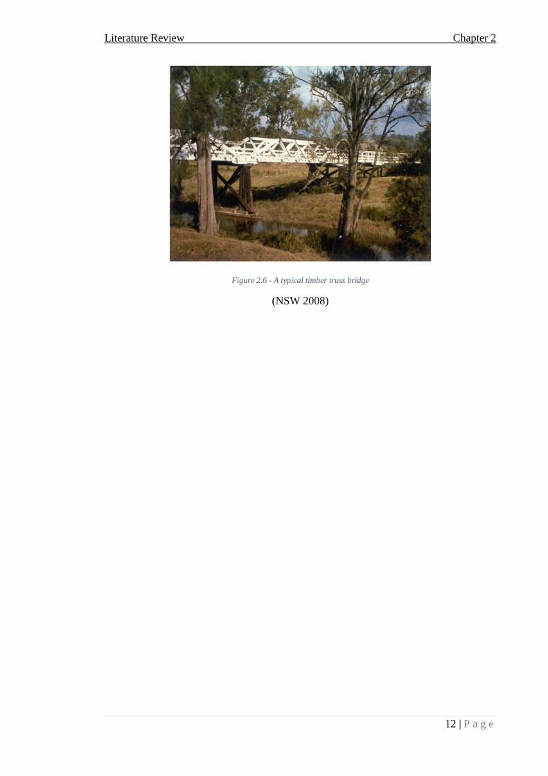
Timber bridges are very uncommon at present due to the significant advantages of steel
and concrete bridges. Due to the weak structure of timber, it is generally only built in
areas with fairly small imposed loads (lightly populated areas).
Literature Review Chapter 2
12 | P a g e
Figure 2.6 - A typical timber truss bridge
(NSW 2008)

Literature Review Chapter 2
13 | P a g e
2.3 Concrete Bridges
2.3.1 General terminology
Most of these terminology definitions have been obtained from the Lichtenberger
Engineering Library (2015).
Abutment: That part of a pier from which an arch springs. A structure sustaining one end
of a bridge span and at the same time supporting the embankment which carries the track
or roadway.
Buckle: To bend in a lateral direction by a longitudinal pressure.
Corrosion: The disintegration of a substance by the action of chemical agents.
Creep: The tendency of a solid material to move slowly or deform permanently under
the influence of mechanical stresses.
Expansion Bearing: A support at the end of a span where provision is made for the
expansion and contraction of the structure.
Expansion Joint: A joint in which movement for expansion and contraction is allowed.
Fatigue: Deformation response over a long period of time caused by repeated cyclic
loading.
Foundation: That portion of a structure, usually below the surface of the ground, which
distributes the pressure upon its support. Also applied to the supporting material itself.
Girder: A beam or compound structure acting as a beam carrying principally transverse
loads which develop normal reactions at the supports.
Pier: A structure, usually composed of masonry, which is used to transmit the loads from
a bridge superstructure to the foundation.
Substructure: The part of any construction which supports the superstructure. The piers,
pedestals, and abutments of a bridge or trestle.
Superstructure: That portion of a bridge or trestle lying above the piers, pedestals, and
abutments. The part of a structure which receives the live load directly (e.g. girders,
beams etc.).
Literature Review Chapter 2
14 | P a g e
Scour: A clearing out or removal of silt and sand in the bed of a stream by a strong
current. To remove such material in that manner.
Thermal Shock: Thermal gradient causes different parts of an object to expand by
different amounts.
Viaduct: An extended bridge of many spans, mainly over dry ground. Usually consists
of alternate towers and open spaces or bays.
Wear: Erosion or sideways displacement from its original position on a solid surface
performed by the action of another surface.
Yielding: The stress at which a material begins to deform plastically, unable to return to
its original shape.
(Library 2015)
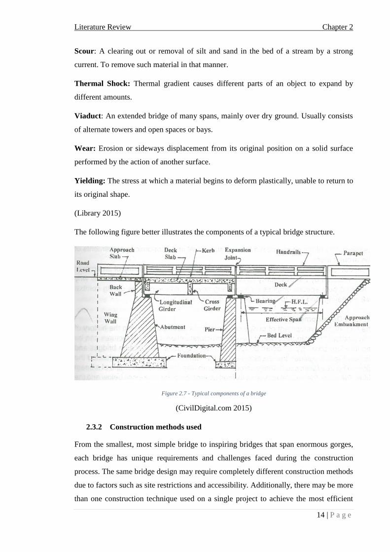
The following figure better illustrates the components of a typical bridge structure.
Figure 2.7 - Typical components of a bridge
(CivilDigital.com 2015)
2.3.2 Construction methods used
From the smallest, most simple bridge to inspiring bridges that span enormous gorges,
each bridge has unique requirements and challenges faced during the construction
process. The same bridge design may require completely different construction methods
due to factors such as site restrictions and accessibility. Additionally, there may be more
than one construction technique used on a single project to achieve the most efficient

Literature Review Chapter 2
15 | P a g e
construction process. While there is no single construction method used for bridges, there
are several broad categories that they fall under.
2.3.2.1 Falsework/staging
There is a common confusion between the difference of formwork and falsework.
Groundforce (2015) describes formwork as “A structure which is usually temporary but
can be whole of part permanent, it is used to contain poured concrete to mould it into
required dimensions and support until it is able to support itself.”
Groundforce (2015) also describes falsework as “any temporary structure, in which the
main load bearing members are vertical, used to support permanent structures, used to
support a permanent structure and associated elements during the erection until it is self-
supporting.”
These two methods can work together in some situations in which falsework can include
temporary support structures for formwork, used to mould concrete to form a desired
shape. This method of construction is generally used in spanning or arched elements in
bridge construction.
Figure 2.8 - Falsework used for a long spanning concrete bridge
(PERI 2015)
2.3.2.2 Incremental Launching
Bridges have been constructed using the incremental launching method for many years
and is a very popular method when constructing bridges over an inaccessible or
environmentally protected obstacle. (LaViolette, Wipf, Lee, Bigelow &Phares 2007)
describes this method as follows:

Literature Review Chapter 2
16 | P a g e
“In this method of construction, the bridge superstructure is assembled on
one side of the obstacle to be crossed and then pushed longitudinally (or
“launched”) into its final position. The launching is typically performed in
a series of increments so that additional sections can be added to the rear
of the superstructure unit prior to subsequent launches.”
The incremental launching method is particularly suited to the construction of continuous
post-tensioned multi-span bridges.
Figure 2.9 - Incremental launching of a bridge
(BBR 2015)
2.3.2.3 Span-by-span
Span-by-span bridge construction offers a very high speed of construction. The two
different types of this method is precast and in-situ, although precast is by far the most
common method of the two. The first step is to erect the segments for the entire span onto
a temporary erection girder, spanning between two piers. Then, the Post-tensions tendons
are installed and stressed; this allows the segments to span on their own. Finally, the
erection girder is advanced into place for the erection of the next span. The most common
use of span-by-span construction is to build long viaducts with spans ranging from 25-
45m.(BBR 2015)

Literature Review Chapter 2
17 | P a g e
Figure 2.10 - Span-by-span construction of a bridge
(Rohleder 2015)
2.3.2.4 Balanced cantilever
“Free cantilevering is a method of construction where a structure is built outward
from a fixed point to form a cantilever structure, without temporary support, using
staged cast-in-situ construction. When two opposing free cantilever structures are
attached as a single structure and erected in the same step, it is known as ‘balanced
cantilever’.” (BBR 2015)
There are two different methods of balanced cantilever bridge construction which are
cast-in-situ and precast. Cast-in-situ is the process whereby segments are progressively
cast in their final positions on site. However, for precast construction, the segments have
already been prefabricated at a casting plant and then transported on-site and erected as a
complete unit in their final positions. They can be precast on-site or at a remote facility.
The balanced cantilever method is often appropriate and cost-effective for the
construction of long span concrete bridges in situations where height, topography and/or
geotechnical conditions render the use of the conventional formwork method
uneconomical.
2.3.3 Types of bridges
Throughout history, engineers and architects have devised many ways of building
bridges, there are many different designs that all serve a unique purpose, each of which
apply to different situations. Bridges may be classified by how the forces of tension,
compression, bending, torsion and shear are distributed throughout the structure. Most

Literature Review Chapter 2
18 | P a g e
bridges will employ all of the principal forces to some degree but in most circumstances
only a few will be dominant.
2.3.3.1 Arch bridges
Arch bridges are one of the oldest types of bridges and have been around for thousands
of years, mainly because of their simplicity and effectiveness. They are still a very
common type of bridge used within the industry. Arch bridges derive their strength from
the fact that vertical loads on an arch generate compressive forces in the arch ring. This
is great for concrete bridges as concrete is very weak in tension. The arch cannot be too
long however or the arch may collapse in on itself, this is when several arches should be
used.
Figure 2.11 – Long-span arch bridge
(Group 2015)
2.3.3.2 Reinforced slab bridges
For short spans, a reinforced concrete slab, generally cast in-situ rather than precast, is
the simplest design. It is also cost-effective, since the flat, level soffit means that
falsework and formwork are also simple. The steel reinforcement is also uncomplicated.
With larger span bridges, the reinforced slab has to be thicker to carry the extra stresses.
This extra self-weight of the slab itself can then become a problem. This can be solved in
one of two ways; the first is to use prestressing techniques and the second is to reduce the
self-weight of the slab by including voids, often expanded polystyrene cylinders. Voided
slabs are generally more economical than prestressed slabs up to about a 25m span.
(Group 2015)

Literature Review Chapter 2
19 | P a g e
Figure 2.12 - Reinforced slab bridge
(Group 2015)
2.3.3.3 Beam and slab bridges
Beam and slab bridges are one of the most common types of concrete bridges thanks to
the success of standard precast prestressed concrete beams being developed, which were
then later developed to the ‘Y’ beam. They are simple, economic, quick to erect and are
widely available in the industry. The precast beams are placed on the supporting piers or
abutments, usually on rubber bearings which are maintenance free. An in-situ reinforced
concrete deck slab is then cast on permanent shuttering which spans between the beams.
(Group 2015)
Figure 2.13 - Beam and slab bridge in construction

Literature Review Chapter 2
20 | P a g e
(Group 2015)
2.3.3.4 Box girder bridges
For spans greater than around 45 metres, prestressed concrete box girders are the most
common method of concrete bridge construction. The main spans are hollow and the
shape of the 'box' will vary from bridge to bridge and along the span, being deeper in
cross-section at the abutments and piers because they are taking a considerable amount
of the stresses and shallower at the midspan due to the significant increase in stress.
Figure 2.14 - Box girder bridge in construction
(Construction 2015)
2.3.3.5 Integral bridges
One of the difficulties in designing any structure is deciding where to put the joints. These
are necessary to allow movement as the structure expands due to the heat in summer and
contracts during the cold of winter. Previous expansion joints and bearings used in these
type of bridges proved to be very unreliable and not very cost effective, therefore more
and more bridges are being built without either. Such structures, called 'integral bridges',
can be constructed with all types of concrete deck. They are constructed with their decks
connected directly to the supporting piers and abutments. Thermal movement of the deck
is accommodated by flexure of the supporting piers and horizontal movements of the
abutments, with elastic compression of the surrounding soil. Already used for bridges that
span up to 60m, the integral bridge is becoming increasingly popular as engineers and
designers find other ways of dealing with thermal movement. (Group 2015)

Literature Review Chapter 2
21 | P a g e
2.3.3.6 Cable-stayed bridges
For very large span bridges, one solution is the cable-stayed bridge. As characterized by
the Dee River Crossing where all elements are concrete, the design consists of supporting
towers carrying cables which support the bridge from both sides of the tower. Generally,
cable-stayed bridges are built using a form of cantilever construction which can be either
in-situ or precast. (Group 2015)
Figure 2.15 - Dee River Crossing cable-stayed bridge
(LUSAS 2013)
2.3.3.7 Suspension bridges
“A suspension bridge is fundamentally simple in action: two cables are suspended
between two supports (‘towers’ or ‘pylons’), hanging in a shallow curve, and a
deck is supported from the two cables by a series of hangers along their length.
The cables and hangers are in simple tension and the deck spans transversely and
longitudinally between the hangers. In most cases the cables are anchored at
ground level, either side of the main towers; often the side spans are hung from
these portions of the cables.” (SteelConstruction.info 2015)
While suspension bridges mainly consist of steel, the concrete used plays a vital role.
There will be massive foundations, usually embedded in the ground, that support the
weight and cable anchorages. Also, the abutments provide the vital strength and ability
to resist the enormous forces. Finally, the superstructures carrying the upper ends of the
supporting cables are generally made from reinforced concrete. (Group 2015)

Literature Review Chapter 2
22 | P a g e
Figure 2.16 - Suspension bridge
(Group 2015)
2.3.4 Design life
As described in the Australian Standards AS 5100.1 - 2004 – Bridge Design, Part 1:
Scope and General Principles
“The design life of structures covered by this standard shall be 100 years.
Elements such as bearings and expansion joints shall be designed to have a long life,
compatible with the design life of the bridge. Provision shall be made for easy removal
and replacement of such elements, and any fixings shall be detailed to be reusable.”
(Standards 2004a)
2.3.5 Modes of failure
Some of the most expensive engineering projects in history have involved building
bridges. Although the fundamentals of bridge-building have been established for
thousands of years, every bridge presents complicated factors that must be taken into
consideration, such as the geology of the surrounding area, the amount of traffic, weather,
construction materials and much more. Occasionally these factors are miscalculated or
not taken into account, or something occurs that the bridge designers didn't expect. The
result can be tragic. Below are the possible broad failure modes that can occur within
concrete bridge structures.
Literature Review Chapter 2
23 | P a g e
2.3.5.1 Mechanical failure
Mechanical failures often occur due to an overload of stress, causing a component of a
bridge to fracture or even fail. Mechanical failure is a common failure mode which
generally occur as a result of buckling, corrosion, creep, fatigue, fracture, impact,
mechanical overload, cracking, thermal shock, wear and yielding. It is common for
mechanical failure to occur due to a combination of these failure modes.
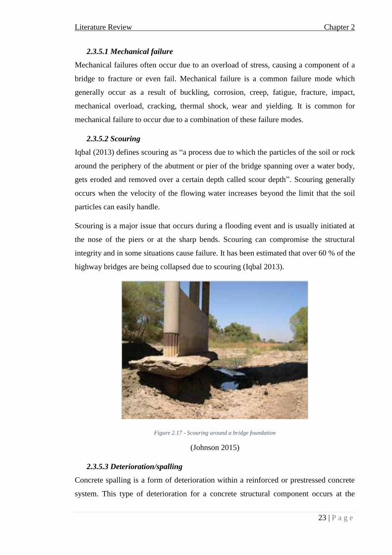
2.3.5.2 Scouring
Iqbal (2013) defines scouring as “a process due to which the particles of the soil or rock
around the periphery of the abutment or pier of the bridge spanning over a water body,
gets eroded and removed over a certain depth called scour depth”. Scouring generally
occurs when the velocity of the flowing water increases beyond the limit that the soil
particles can easily handle.
Scouring is a major issue that occurs during a flooding event and is usually initiated at
the nose of the piers or at the sharp bends. Scouring can compromise the structural
integrity and in some situations cause failure. It has been estimated that over 60 % of the
highway bridges are being collapsed due to scouring (Iqbal 2013).
Figure 2.17 - Scouring around a bridge foundation
(Johnson 2015)
2.3.5.3 Deterioration/spalling
Concrete spalling is a form of deterioration within a reinforced or prestressed concrete
system. This type of deterioration for a concrete structural component occurs at the

Literature Review Chapter 2
24 | P a g e
surface where concrete will decompose, often leaving any steel reinforcement visible and
open to additional corrosion. Spalling is typically a result of reinforcement corrosion or
joint failure.
Concrete spalling is a serious and common issue within bridge structures. It begins at
either the concrete or steel reinforcement level, where chemical-physical effects will
occur. Typical forms of reaction include: calcium chloride with concrete, sulphate attack
on concrete, chloride penetration to steel, and the carbonation process (Friend 2013).
Certain environments can intensify the process, so appropriate consideration must be
taken in the design process.
Figure 2.18 - Deterioration of an overpass
(Friend 2013)
2.3.6 How they are maintained
Concrete structures gradually deteriorate over an extended period of time, requiring
maintenance to be performed. It is generally a long-term process as the rate of
deterioration is dependent on a number of different variables. These include the amount
of time the structure has been in service, the specific function of the structure, the
activities that are conducted within/on the structure, the environmental conditions in
which the structure is situated in as well as the physical properties of the concrete used
(Rashidi et al. 2010).

Literature Review Chapter 2
25 | P a g e
The most common problems encountered that require maintenance are corrosion of steel
reinforcement, structural deficiency, chemical/acid attack, frost damage, fire damage,
creep, internal reaction within the concrete, restrained movement, cracking and
mechanical damage (Rashidi et al. 2010).These problems can develop suddenly or
gradually over a long period of time.
A long, successful bridge program is based on a strategic, systematic and balanced
approach. The U.S. Department of Transportation (2011) splits the maintenance of a
bridge up into two broad categories, these are:
1. Preventative maintenance
2. Rehabilitation
2.2.3.1 Preventative maintenance
Preventative maintenance is intended to delay the need for costly reconstruction or
replacement actions by applying preservation strategies on bridges as long as possible
while they are still in good condition. This maintenance is typically applied to elements
of components of a bridge with significant remaining useful life. Some examples of
preventative maintenance activities are bridge washing/cleaning, sealing deck joints,
facilitating drainage, sealing concrete, painting steel, removing channel debris, protecting
against scour and lubricating bearings (U.S Department of Transportation 2011).
2.2.3.2 Rehabilitation
Rehabilitation is intended to restore the structural integrity of a bridge and correct major
safety defects. Rehabilitation projects provide complete or near complete restoration of
bridge elements/components. These projects generally require significant engineering
resources, a lengthy completion schedule and are very costly. Some examples of bridge
rehabilitation are deck replacement, superstructure replacement and strengthening (U.S
Department of Transportation 2011).

Literature Review Chapter 2
26 | P a g e
2.4 Natural Disasters
2.4.1 Flooding
“Floods are part of the natural water cycle or a “Hydrologic Cycle”. In this natural
cycle, the energy of the sun causes water to evaporate and form clouds, which
move inland and become rain. This rain will then runoff either directly through
the river systems or be absorbed into the soil to later form groundwater flow.
Floods happen when the capacity of the rivers is not enough to carry the water
that has entered the river network, and the banks overflow. ” (BOM 2015)
Flooding is considered a complex, natural phenomenon due to its unpredictable nature.
This is mainly due to the different factors that affect the size of flooding. Some examples
are rainfall intensity, rainfall duration, how wet or dry the land is, topography and ground
cover.
In Australia, the most common forms of flooding are:
Slow-onset flooding
Rapid-onset flooding
Flash flooding
2.4.1.1 Slow-onset flooding
Slow-onset floods usually occur on inland rivers such as those found in central and
western New South Wales, central and western Queensland and parts of Western
Australia. As the name suggests, these floods are very slow to develop, take at least a
week to develop and can persist for months. As heavy rain falls, the river is unable to
accommodate the extra water storage and as a result, causes the river to overflow its
banks. Slow-onset floods can result in damage to crops, livestock, rail lines, roads and
property. (BOM 2015)
2.4.1.2 Rapid-onset flooding
Rapid-onset floods occur more quickly, but they can be more catastrophic since there is
less warning than with slow-onset floods. Rapid-onset floods occur on rivers in coastal
and mountain. Since these rivers drain more quickly than slow-moving inland rivers,
flooding happens more quickly, generally over 2-3 days. (BOM 2015)

Literature Review Chapter 2
27 | P a g e
2.4.1.3 Flash flooding
Flash floods occur when the local drainage systems, either natural or man-made, cannot
accommodate the extreme intensity of the rainfall. These floods occur with little or no
warning, and as a result, are far more dangerous than the other two flood types. Flash
floods are an increasing problem in cities which have poor drainage (BOM 2015). The
2011 Toowoomba floods is a prime example of how deadly they can be.
2.4.1.4 Bridge failures due to flooding
Floods can cause bridges to collapse in a few different ways. Severe floods, such as rapid-
onset and flash flooding, can cause rivers and creeks to overflow, picking up debris such
as trees, cars and parts of houses in the process. When the river passes under a bridge, the
high water level smashes the debris into the bridge. The shear impact of the debris can
cause immediate bridge failure, or the weight of the debris piled up combined with the
immense force of the fast-flowing water pushing on it can cause the bridge to fail more
gradually.
Flooding can also cause bridges to fail by gradually wearing away the earth around and
underneath the bridge piers. This process is known as scouring, and is a serious issue to
consider whenever bridge foundations are placed underwater. The natural flow of the
water can produce scour over many years, but bridges are designed to withstand this.
However, in the event of floods, the enormous increase in force and volume of water
affecting the bridge and damage to the foundation soil can cause a bridge to collapse
immediately or very gradually.
Figure 2.19 - Bridge collapse cause by Cumbria floods
(BBC 2009)

Literature Review Chapter 2
28 | P a g e
2.4.2 Earthquake
Earthquakes are caused by the Earth naturally releasing stress within the crust. This
release of stress usually occurs when two blocks of earth slip past one another. As these
plates move past each other, the stress is released as energy which moves through the
Earth in the form of waves, which cause the surrounding surface to vibrate. (Subranami
et al. 2014)
Earthquakes occur throughout the world, but the vast majority occurs along narrow belts
which can be tens to hundreds of kilometres wide. These belts mark boundaries (also
known as plate boundaries) on the planet's surface that are very geologically active.
Intraplate earthquakes are less common. These take place in relatively stable areas, away
from plate boundaries. This type of earthquakes generally originate at more shallow levels
of the Earth’s crust. Fortunately, due to the geological position, Australia is only prone to
intra-plate earthquakes and hence doesn’t have to worry a great deal about a disaster
occurring. (Subranami et al. 2014)
Major earthquakes can cause dozens of buildings to collapse, but collapsed bridges are
often the most visible signs of the havoc an earthquake can cause. Fortunately,
earthquake-triggered bridge collapses are relatively rare. To combat this issue, bridges
can be designed in earthquake-prone areas to withstand tremors (for example, Japan), or
at least minimize the loss of life when one occurs. The following figure shows the
devastating effects that earthquakes can have on bridges.
Figure 2.20 - Complete collapse of a bridge in Santiago due to an earthquake
(Subranami et al. 2014)

Literature Review Chapter 2
29 | P a g e
2.4.3 Cyclone
Cyclones are low pressure systems that form off the coast over warm tropical waters.
They form when there is a combination of warm water (above 26.5°C), high relative
humidity and increased precipitation. This in turn drives atmospheric energy to form a
cyclone. They are extremely dangerous because they produce destructive winds, heavy
rainfall (which can cause major flooding) as well as damaging storm surges that can
inundate low-lying coastal areas (which can cause serious erosion of foreshores). Once
formed, they can persist for many days and follow unpredictable paths. Cyclones will
usually dissipate when they travel inland or across colder oceans as their driving forces
decrease. (BOM 2015)
The Bureau of Meteorology (2015) has created five categories for identifying the severity
of a cyclone, depending on the wind speed that they exert, these can be seen in table 2.1:
Table 2.1 - Cyclone categories
(BOM 2015)
The main effects of tropical cyclones include heavy rainfall, strong winds and large storm
surges, all of which can lead to major damage to bridges. The sheer force of these strong
winds can tear a bridge apart that are not built to withstand this. Furthermore, all of the
loose debris that are picked up along the path of destruction can turn these debris into
deadly flying projectiles and can cause very large impact damage. Also, the heavy rainfall
associated with tropical cyclones can cause major flooding of rivers. The loose debris can
also be thrown into these rivers; this accumulation of debris and increased flow rate of
water along the channel can cause major damage to bridges. Finally, storm surges along
coastal areas are generally the worst effect from cyclones and have the most potential for
damage to infrastructure. The quick surge in sea level coupled with the heavy rainfall and
strong winds can be lethal. Figure 2.21 shows how destructive cyclones can be to bridges
that span cross rivers.

Literature Review Chapter 2
30 | P a g e
Figure 2.21 - A blown away bridge cause by Cyclone Hudhud
(Navy 2014)
2.4.4 Bushfire
Skwirk (2015) defines a bushfire as “a wildfire that burns out of control spreading across
vegetated regions of bushland”. In order for a bushfire to be catastrophic, the right
conditions must be present. Most bushfires happen in times when temperatures are high
and the conditions are dry. Areas with dense undergrowth, as can be found in south-
eastern Australia, are the most vulnerable to bushfire. New South Wales and Victoria
experience bushfires more then any other part of Australia. Bushfires often start when dry
winds blow inland from central Australia. While the winds bring dry weather, they also
provide ventilation for the flames. Dry leaves and bark are especially flammable. Also,
trees such as eucalypts are especially prone to fire because their leaves have a highly-
flammable oil (Skwirk 2015).
The Queensland Government (2015) has created a rating scale to indicate the potential
for danger that a fire poses, these can be seen in table 2.2:

Literature Review Chapter 2
31 | P a g e
Table 2.2 - Queensland fire danger categories
(Government 2015)
Fire might be one of the rarest causes of bridge failure, but given the right circumstances,
it may cause a great deal of damage to a bridge. This was a very big issue for bridge
design when timber was still a popular choice of material and bushfires present a serious
threat for timber bridges. Train bridges were especially susceptible to fire, because the
steel wheels of the train on the steel rails of the track frequently sent sparks shooting onto
the bridge. If it was very dry or the wind fanned the sparks, the bridge could catch fire
and completely burn down.
Bridge fires can still currently cause major damage to bridges. Several modern bridges
have also collapsed or been severely damaged due to fire. This is typically due to very
large explosions, for example, the crash of a tanker truck carrying a large amount of a
highly flammable substance like petrol. The crash may trigger an explosion and a blaze
with such a high temperature, it can melt the steel used to build the bridge. In some
situations, this can lead to complete failure, as illustrated in figure 2.22 when a 303m
bridge in Asia was destroyed by a raging fire.

Literature Review Chapter 2
32 | P a g e
Figure 2.22 - Destruction of the Feng Yu Bridge in China
(Blake 2013)

Literature Review Chapter 2
33 | P a g e
2.5 Extreme flood events in Australia
2.5.1 Summer 2010/2011 Queensland flood events
The 2010/2011 summer in Queensland was not the wettest in history but was notable for
the fact that over 80% of the state was declared a natural disaster area. The constant heavy
rain throughout the summer ended with a climax when the category 5 Cyclone Yasi
hammered northern Queensland. Cyclone Yasi had wind gusts up to 285km/h and caused
a 5m tidal surge. (Pritchard 2013)
The most critical flooding event occurred on the 13th January 2011. Major flooding
occurred throughout most of the Brisbane River catchment but the most severe flooding
occurred in Toowoomba and the Lockyer Creek catchment. The flooding caused the loss
of 23 lives in the Lockyer Valley and one in Brisbane; an estimated 18000 properties were
inundated in the Brisbane CBD, Ipswich and along the Brisbane River Valley. (Honert &
McAneney 2011)
The damage to the bridge network included:
Two timber bridges requiring replacement due to severe flood damage
One bridge registering 70 mm pier settlement.
One concrete bridge downstream of the dams on the North Pine River system
having 4m scouring at the river piers due to overtopping of the bridge. Subsequent
load testing of the bridge showed there was significant reduction in the pile
capacity of the bridge. It was determined that replacement of this bridge was the
most economical outcome.
A steel girder bridge on the Mitchell River requiring replacement due to scour of
the piers.
Scouring of numerous abutments spill-through embankments.
Many bridge approaches being washed out.
(Pritchard 2013)
Lockyer Valley residents identified vegetation and debris remaining in waterways as a
major concern should further flooding occur and were a major contributing factor to the
damage of the bridge network (n.a). During the January flood, items picked up by the
torrents of water were a serious danger to life and property as they were carried at speed

Literature Review Chapter 2
34 | P a g e
downstream, and blocked the escape of water as they were caught against culverts and
bridges. This blockage disrupted the natural flow of water and caused water to back up,
resulting in further load damage and bridge scouring.
Figure 2.23 - Urban debris being thrown into a bridge
(Pritchard 2013)
Figure 2.24 - Scoured road approach at bridge abutment
(Pritchard 2013)
2.5.2 2013 Queensland flood events (Cyclone Oswald)
In January 2013, Tropical Cyclone Oswald passed over south-east Queensland and parts
of New South Wales, resulting in widespread severe storms, flooding and water spouts.
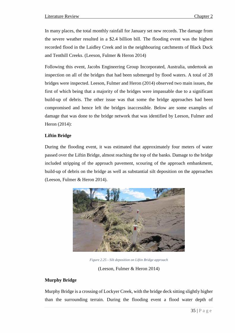
Literature Review Chapter 2
35 | P a g e
In many places, the total monthly rainfall for January set new records. The damage from
the severe weather resulted in a $2.4 billion bill. The flooding event was the highest
recorded flood in the Laidley Creek and in the neighbouring catchments of Black Duck
and Tenthill Creeks. (Leeson, Fulmer & Heron 2014)
Following this event, Jacobs Engineering Group Incorporated, Australia, undertook an
inspection on all of the bridges that had been submerged by flood waters. A total of 28
bridges were inspected. Leeson, Fulmer and Heron (2014) observed two main issues, the
first of which being that a majority of the bridges were impassable due to a significant
build-up of debris. The other issue was that some the bridge approaches had been
compromised and hence left the bridges inaccessible. Below are some examples of
damage that was done to the bridge network that was identified by Leeson, Fulmer and
Heron (2014):
Liftin Bridge
During the flooding event, it was estimated that approximately four meters of water
passed over the Liftin Bridge, almost reaching the top of the banks. Damage to the bridge
included stripping of the approach pavement, scouring of the approach embankment,
build-up of debris on the bridge as well as substantial silt deposition on the approaches
(Leeson, Fulmer & Heron 2014).
Figure 2.25 - Silt deposition on Liftin Bridge approach
(Leeson, Fulmer & Heron 2014)
Murphy Bridge
Murphy Bridge is a crossing of Lockyer Creek, with the bridge deck sitting slightly higher
than the surrounding terrain. During the flooding event a flood water depth of

Literature Review Chapter 2
36 | P a g e
approximately two meters was estimated on the northern approach. Damage to the bridge
included stripping of the approach pavement, deposition of silt on the approaches as well
as a significant build-up of debris on the bridge deck (Leeson, Fulmer & Heron 2014).
Figure 2.26 – Damage to the Murphy Bridge
(Leeson, Fulmer & Heron 2014)
The Willows Bridge
The Willows Bridge is another crossing of Lockyer Creek, with the bridge deck sitting
slightly higher than the surrounding flood plain. During the flood event, it was estimated
that the flood water depth was approximately two meters above the bridge level. Damage
to the bridge included stripping of the approach pavement, complete scour through both
abutments, removal of bridge rails and a build-up of debris on the bridge deck.
Figure 2.27 - Damage to the Willows Bridge
(Leeson, Fulmer & Heron 2014)

Literature Review Chapter 2
37 | P a g e
2.6 Forces exhibited during a flooding event
2.6.1 Hydrostatic pressure
When a solid is submerged in water, water pressure is applied to the object. The pressure
at any particular point is a function of the height of the fluid in consideration and the fluid
density. The basic pressure equation is:
𝑃 = 𝜌𝑔ℎ
Where:
ρ = water density (kg/m3)
g = gravitational acceleration = 9.81 m/s2
h = height of the fluid
Consider the submerged object below:
Figure 2.28 - Pressure prism of a submerged object
(Saskatchewan 2015)
The pressure prism can be equated to a resultant force, Fr, which acts through Cp, the
centre of pressure. The reason that the pressure prism is represented as a triangle is due
to the fact that the least amount of pressure being applied is at the water surface (h=0,
P=0). As the distance is increased into the water, pressure is applied to the wall and the
pressure above is applied to the point below, therefore the pressure keeps increasing in a
linear fashion. The deeper an object in submerged in a fluid, the more pressure will be
applied to the object at the deepest point.

Literature Review Chapter 2
38 | P a g e
2.6.2 Buoyancy
When an object is placed in water, the water exerts an upward force. Buoyancy can be
defined as the upward force that an object feels from the water and when compared to the
weight of the object, it is what makes an object float, sink or remain neutrally buoyant in
the water. When the object floats, the buoyant force is greater than the downward force
of the object.
Figure 2.29 - A floating object
(Seaperch 2015)
When an object sinks, the weight of the object overcomes the upward buoyant force.
Figure 2.30 - A sinking object
(Seaperch 2015)
When an object is neutrally buoyant, the object has the same density as water and neither
floats nor sinks.
Figure 2.31 - A neutrally buoyant object
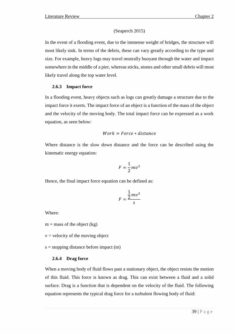
Literature Review Chapter 2
39 | P a g e
(Seaperch 2015)
In the event of a flooding event, due to the immense weight of bridges, the structure will
most likely sink. In terms of the debris, these can vary greatly according to the type and
size. For example, heavy logs may travel neutrally buoyant through the water and impact
somewhere in the middle of a pier, whereas sticks, stones and other small debris will most
likely travel along the top water level.
2.6.3 Impact force
In a flooding event, heavy objects such as logs can greatly damage a structure due to the
impact force it exerts. The impact force of an object is a function of the mass of the object
and the velocity of the moving body. The total impact force can be expressed as a work
equation, as seen below:
𝑊𝑜𝑟𝑘 = 𝐹𝑜𝑟𝑐𝑒 ∗ 𝑑𝑖𝑠𝑡𝑎𝑛𝑐𝑒
Where distance is the slow down distance and the force can be described using the
kinematic energy equation:
𝐹 =1
2𝑚𝑣2
Hence, the final impact force equation can be defined as:
𝐹 =
12 𝑚𝑣2
𝑠
Where:
m = mass of the object (kg)
v = velocity of the moving object
s = stopping distance before impact (m)
2.6.4 Drag force
When a moving body of fluid flows past a stationary object, the object resists the motion
of this fluid. This force is known as drag. This can exist between a fluid and a solid
surface. Drag is a function that is dependent on the velocity of the fluid. The following
equation represents the typical drag force for a turbulent flowing body of fluid:

Literature Review Chapter 2
40 | P a g e
𝐹𝐷 =1
2𝜌𝑣2𝐶𝐷𝐴
ρ = fluid density (kg/m3)
v = fluid velocity (m/s)
CD = drag coefficient, which varies according to the shape of the object that is resisting
the flow of water
A = cross-sectional area of the object that the fluid is acting on
In the event of a flood, there can be a drag force exhibited in more than one direction at a
time. In this instance, the “drag force” is the drag force component that acts parallel to
the direction of the flow, whereas the drag force component that acts perpendicular to the
direction of flow is known as a “lift force”. It should be noted that the lift force can act
both horizontally and vertically.

Australian Bridge design standards Chapter 3
41 | P a g e
CHAPTER 3 AUSTRALIAN BRIDGE DESIGN
STANDARDS
3.1 Chapter overview
This chapter identifies the flood loadings that are outlined in the Australian Bridge Design
Standards, AS5100, 2004. Fluid forces will first be identified, for all submergence
conditions. This will be followed by traffic loads for the partial submergence case.
Finally, the recommended load combinations will be identified from the standards.
3.2 Introduction
The following information throughout this chapter has been extracted from AS 5100.2,
2004.
As described in AS5100.1 - Part 1: Scope and General Principles (Standards 2004a):
When a bridge crosses a river, stream or any other body of water, it shall be designed
to resist the effects of water flow and wave action, as applicable. The design shall
include an assessment of how the water forces may vary in an adverse manner under
the influence of debris, log impact, scour and buoyancy of the structure.
Tidal and wave actions shall be considered on bridges across large bodies of water,
estuaries and open sea.
3.3 Fluid forces on piers
The main forces that need to be taken into consideration in the design of bridge piers are
the drag force and lift force, as shown in figure 3.1:

Australian Bridge design standards Chapter 3
42 | P a g e
Figure 3.1 - Drag and lift forces on piers
(Standards 2004b)
3.3.1 Drag force
In bridge structures subjected to water flow effects, the design drag forces parallel to the
plane containing the pier shall be calculated as follows:
𝐹𝑑𝑢∗ = 0.5𝐶𝑑𝑉𝑢
2𝐴𝑑
Where:
Cd = drag coefficient, depending upon pier shape
In the absence of more exact estimates, Cd shall be calculated as follows:
Cd = 0.7 (semi-circular pier nosing)
= 1.4 (square end pier nosing)
= 0.8 (wedge, sharper than 90°, nosing)
Vu = mean velocity of water flow for ultimate limit states at the level of the
superstructure or debris as appropriate
Ad = area,
= (thickness of pier normal to the direction of the water flow) x (height of water
flow)

Australian Bridge design standards Chapter 3
43 | P a g e
3.3.2 Lift forces
The design lift forces, perpendicular to the plane containing the pier shall be calculated
as follows:
𝐹𝐿𝑢∗ = 0.5𝐶𝐿𝑉𝑢
2𝐴𝐿
Where:
CL = lift coefficient, which depends on the angle between the water flow direction
and the plane containing the pier. In the absence of more exact estimates, it shall be
calculated as follows:
CL = 0.9 for θw ≤ 30°
= 1.0 for θw > 30°
Where θw is the angle between the direction of the water flow and the transverse centre-
line of the pier.
AL = area,
= (width of the pier parallel to the direction of the water flow) x (height of the flow)
3.3.3 Debris forces
𝐹𝑑𝑢∗ = 0.5𝐶𝑑𝑉𝑢
2𝐴𝑑𝑒𝑏
Where:
Adeb = projected area of debris
Cd = drag coefficient, which can be obtained from figure 3.2:

Australian Bridge design standards Chapter 3
44 | P a g e
Figure 3.2 - Pier debris Cd
(Standards 2004b)
3.4 Fluid forces on superstructures
The main considerations that need to be taken into consideration for the design of bridge
superstructures are drag forces, lift forces and the moment.
3.4.1 Drag force
𝐹𝑑𝑢∗ = 0.5𝐶𝑑𝑉𝑢
2𝐴𝑠
Where:
As = wetted area of the superstructure, including any railings or parapets, projected on a
plane normal to the water flow
Cd = drag coefficient, which can be obtained from figure 3.3:
Figure 3.3 - Superstructure Cd
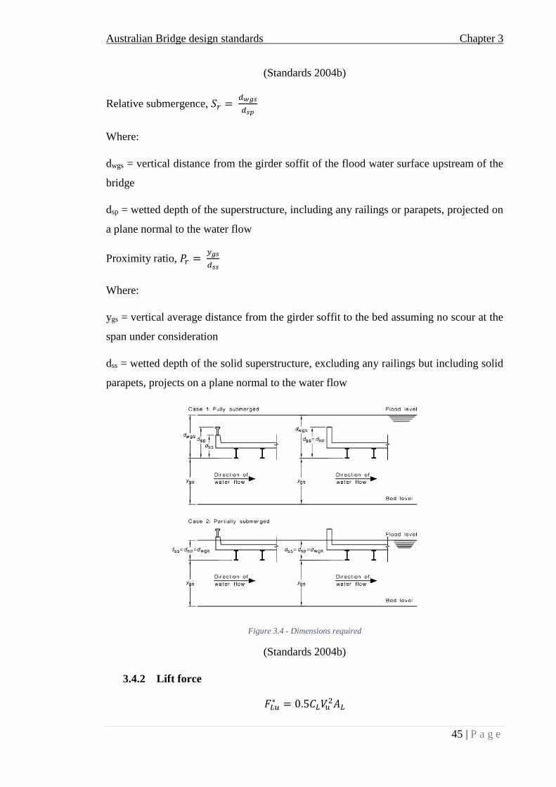
Australian Bridge design standards Chapter 3
45 | P a g e
(Standards 2004b)
Relative submergence, 𝑆𝑟 = 𝑑𝑤𝑔𝑠
𝑑𝑠𝑝
Where:
dwgs = vertical distance from the girder soffit of the flood water surface upstream of the
bridge
dsp = wetted depth of the superstructure, including any railings or parapets, projected on
a plane normal to the water flow
Proximity ratio, 𝑃𝑟 = 𝑦𝑔𝑠
𝑑𝑠𝑠
Where:
ygs = vertical average distance from the girder soffit to the bed assuming no scour at the
span under consideration
dss = wetted depth of the solid superstructure, excluding any railings but including solid
parapets, projects on a plane normal to the water flow
Figure 3.4 - Dimensions required
(Standards 2004b)
3.4.2 Lift force
𝐹𝐿𝑢∗ = 0.5𝐶𝐿𝑉𝑢
2𝐴𝐿

Australian Bridge design standards Chapter 3
46 | P a g e
Where:
CL = lift coefficient, which shall be obtained from figure 3.5:
Figure 3.5 - Superstructure CL
(Standards 2004b)
Two lift forces shall be calculated at each Sr. The upper value of CL shall be used when
determining the resistance of the structure to overturning and the tie down requirements.
The lower value of CL (downward force) will be considered in the design of a deck,
girders, substructures and foundations.
3.5 Debris forces
𝐹𝑑𝑢∗ = 0.5𝐶𝑑𝑉𝑢
2𝐴𝑑𝑒𝑏
Where:
Adeb = projected area of debris
Cd = drag coefficient, which can be obtained from figure 3.7:

Australian Bridge design standards Chapter 3
47 | P a g e
Figure 3.6 - Superstructure debris Cd
3.6 Effects due to logs
Where floating logs are a possibility, the design forces (ultimate and serviceability)
exerted by the logs directly hitting piers or superstructures shall be calculated on the
assumption that a log has a minimum mass of 2t (2000kg) and will be stopped in a
distance of:
1) 150mm for hollow concrete piers
2) 75mm for solid concrete piers
If fender piles or sheathing are placed upstream from the pier to absorb the energy of the
blow, the stopping distance shall be increased. The design forces will be calculated using
the mean velocity of water flow at flood level Vs for serviceability, or Vu for ultimate
limit states.
The forces due to log impact shall not be applied concurrently but they should be applied
with other water flow forces as appropriate.
The following equation shall be used to calculate the impact force of a log:
𝐹𝐿𝑢∗ =
0.5𝑚𝑉𝑢2
𝑠
Where:
m = mass of the log
s = stopping distance (m)
(Toolbox 2015)

Australian Bridge design standards Chapter 3
48 | P a g e
3.7 Effects due to buoyancy
In assessing the effects of buoyancy and lift on bridge structures, the effects of buoyancy
and lift on substructures (piling) and superstructures shall be given consideration.
Buoyancy shall be applied concurrently with other water flow forces as appropriate.
For beam and slab or box girder bridges, several horizontal bleed holes with a minimum
diameter of 75mm will be provided in webs or diaphragms, or both. Similarly, vertical
bleed holes with a minimum diameter of 50mm should be provided in the deck to dissipate
air which may be trapped between the high water level and the underside of the deck slab.
Where upward lift forces are possible (that is buoyancy is contributing), a positive tie-
down system should be provided.
In this case, the ultimate force = 1.5𝐹𝐿𝑢∗ + 𝐵 − 𝛾𝑔𝐷𝐿
Where:
B = Bouyancy
DL = dead load
𝛾𝑔 = lower value given in figure 3.8:
Table 3.1 - Load factors for dead loads
(Standards 2004b)
3.8 Effects due to debris
Debris forces should not be used concurrently with water flow forces except in the case
of determining the resistance of the structure to overturning. In this case, an upward lift

Australian Bridge design standards Chapter 3
49 | P a g e
force shall be assumed when the debris is acting on the superstructure. The upward lift
force shall be calculated as follows:
For ultimate design:
𝐹𝐿𝑢∗ = (0.5𝐶𝐿𝑉𝑢
2𝐴𝐿) + 𝐵
Where:
CL = 0.5
AL = area,
= (width of the pier parallel to the direction of the water flow) x (height of the flow)
B = Buoyancy force
3.8.1 Depth of debris mat
The depth of a debris mat varies depending on factors such as catchment vegetation,
available water flow depth and superstructure span. In the absence of more accurate
estimates, the depth shall be estimated somewhere in the range of 1.2 – 3 meters.
3.8.2 Debris acting on piers
A debris load acting on piers shall be considered for bridges where the flood level is
below the superstructure. The length of a debris mat shall be taken as:
𝐿 = (0.5 ∗ ∑ 𝑎𝑑𝑗𝑎𝑐𝑒𝑛𝑡 𝑠𝑝𝑎𝑛𝑠), or 20m, whichever is smaller.
The debris load should be applied at mid-height of the debris mat with the assumption
that the top of the debris mat is at the same level as to flood level.
3.8.3 Debris acting on superstructures
A debris load acting on superstructures should be considered for bridges where the flood
level is above a level of 600mm below the soffit level. The length of the debris mat shall
be the projected length of the superstructure. The debris load shall be applied at the mid-
height of the superstructure, including any railing or parapets.
3.9 Traffic loads
In the event of partial submergence, traffic loads must be taken into account.

Australian Bridge design standards Chapter 3
50 | P a g e
The most likely and most critical traffic scenario is the “M1600 moving traffic load”,
provided in clause 6.2.3 of AS5100.
The M1600 moving traffic load accounts for the loads applied by a moving stream of
traffic. The load is assumed to act within a standard design lane with a width of 3.2m, as
shown in figure 3.9:
Figure 3.7 - M1600 moving traffic loads
(Standards 2004b)
As shown in figure 3.9, the applied traffic loads can be taken as a 360kN load acting over
an area of 2.5m x 2m, as well as a line load of 6kN/m acting through the centre of the
lane. For Tenthill Bridge, there are 2 standard design lanes, therefore table 6.6 shall be
taken into account.
Table 3.2 - Lane load factors
(Standards 2004b)
It is more likely that one lane will be loaded, rather than both lanes being loaded
simultaneously. Furthermore, the most critical effect that the traffic loading will have on
the bridge is when the downstream end is loaded (which will contribute to overturning),
hence only the downstream lane will be loaded for the simulation.

Australian Bridge design standards Chapter 3
51 | P a g e
Following clause 6.7, a dynamic load allowance shall be taken into consideration to
account for the interaction between moving vehicles and the bridge structure. The
dynamic load allowance can be obtained from table 6.7.2, as seen below:
Table 3.3 - Dynamic load allowance
(Standards 2004b)
As the M1600 load is the only load being taken into account, α = 0.3, hence:
𝑀1600 𝑙𝑜𝑎𝑑 = (1 + 𝛼) ∗ 𝑙𝑜𝑎𝑑 𝑓𝑎𝑐𝑡𝑜𝑟 ∗ 𝑎𝑐𝑡𝑖𝑜𝑛 𝑢𝑛𝑑𝑒𝑟 𝑐𝑜𝑛𝑠𝑖𝑑𝑒𝑟𝑎𝑡𝑖𝑜𝑛
Where:
Load factor = 1.0, obtained from figure 3.12:
Table 3.4 - Traffic load factors
(Standards 2004b)
Hence,
𝑇𝑜𝑡𝑎𝑙 𝑡𝑟𝑎𝑓𝑓𝑖𝑐 𝑙𝑜𝑎𝑑 = 1.3 ∗ 𝑀1600 𝑙𝑜𝑎𝑑
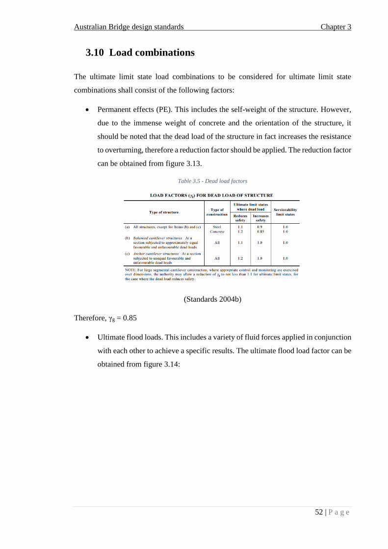
Australian Bridge design standards Chapter 3
52 | P a g e
3.10 Load combinations
The ultimate limit state load combinations to be considered for ultimate limit state
combinations shall consist of the following factors:
Permanent effects (PE). This includes the self-weight of the structure. However,
due to the immense weight of concrete and the orientation of the structure, it
should be noted that the dead load of the structure in fact increases the resistance
to overturning, therefore a reduction factor should be applied. The reduction factor
can be obtained from figure 3.13.
Table 3.5 - Dead load factors
(Standards 2004b)
Therefore, γg = 0.85
Ultimate flood loads. This includes a variety of fluid forces applied in conjunction
with each other to achieve a specific results. The ultimate flood load factor can be
obtained from figure 3.14:

Australian Bridge design standards Chapter 3
53 | P a g e
Figure 3.8 - Ultimate flood load factor
(Standards 2004b)
Therefore, the ultimate factors for each ARI is:
Table 3.6 - Ultimate load factors
For full submergence, the major factors are the permanent effects (structure self-weight)
and the flood loads. That is:
𝐹𝑢𝑙𝑙 𝑠𝑢𝑏𝑚𝑒𝑟𝑔𝑒𝑛𝑐𝑒 = 0.85𝑃𝐸 + 𝑢𝑙𝑡𝑖𝑚𝑎𝑡𝑒 𝑙𝑜𝑎𝑑 𝑓𝑎𝑐𝑡𝑜𝑟 ∗ 𝑓𝑙𝑜𝑜𝑑 𝑙𝑜𝑎𝑑
For partial submergence, traffic loads need to be taken into account, therefore:
𝑃𝑎𝑟𝑡𝑖𝑎𝑙 𝑠𝑢𝑏𝑚𝑒𝑟𝑔𝑒𝑛𝑐𝑒 = 0.85𝑃𝐸 + 𝑢𝑙𝑡𝑖𝑚𝑎𝑡𝑒 𝑙𝑜𝑎𝑑 𝑓𝑎𝑐𝑡𝑜𝑟 ∗ 𝑢𝑙𝑡𝑖𝑚𝑎𝑡𝑒 𝑓𝑙𝑜𝑜𝑑 𝑙𝑜𝑎𝑑 +
𝑠𝑒𝑟𝑣𝑖𝑐𝑒𝑎𝑏𝑖𝑙𝑖𝑡𝑦 𝑡𝑟𝑎𝑓𝑓𝑖𝑐 𝑙𝑜𝑎𝑑

International Bridge Design Standards Chapter 4
54 | P a g e
CHAPTER 4 INTERNATIONAL BRIDGE
DESIGN STANDARDS
4.1 Chapter overview
This chapter identifies the relevant flood loadings from International Bridge Design
Standard. It was determined that a standard would be selected from Europe, Asia and
America. Due to limited freely available resources on the internet, the three standards that
were chosen was the British Bridge Design Standard, BA 59/94 (the European standard),
the Indian Code of Practice, 2014 (the Asian standard) and the American Association of
State Highway and Transportation Officials (AASHTO) Load-and-Resistance Factor
Design (LFRD) Bridge Design specifications, 2012 (the American standard). The
following chapter shows the identified flood loadings from the above Standards.
4.2 European Bridge Design Standards (Ba 59/94)
The following information has been extracted from the British Design Manual for Roads
and Bridges, 1994. It should be noted that these standards are fairly old, however this was
the only accessible UK standards available to the author.
4.2.1 Hydrodynamic forces on piers
4.2.1.1 Flow pressure
The equation for the hydrodynamic flow pressure can be seen below:
𝑃 = 0.51𝐾𝑈2
Where:
K is dependent on the pier shape. Recommended K values can be seen in table 4.1:

International Bridge Design Standards Chapter 4
55 | P a g e
Table 4.1 - K values
(The Highways Agency 1994)
U = velocity of the current at the point where pressure intensity is being calculated. U is
assumed to vary linearly from 0 (at the point of deepest scour) to a maximum (at the free
water surface).
It should be noted that this method is only applicable for circumstances where the water
is flowing perpendicular to the piers. If the current strikes the pier at an angle, the drag
and lift coefficients must be used.
4.2.1.2 Drag force
The drag force acting parallel to the direction of flow can be calculated using the equation
below:
𝐹𝐷 = 𝐶𝐷𝜌𝑈𝑜
2𝑦𝑜𝐿
2000
Where:
U = approach flow velocity (m/s)
yo = depth upstream of the pier (m)
L = length of the pier (or pier diameter for single cylindrical pier) (m)
ρ = water density (kg/m3)
The drag coefficients aren’t provided in this standard, the coefficients are provided in a
separate paper in chart form. Since there are only few coefficients for rectangular-faced
piers, the charts from the recommended paper cannot be used accurately. However, an
example was given for a case study in the standard, therefore the coefficients in this
example was used.

International Bridge Design Standards Chapter 4
56 | P a g e
Cd = 0.4
4.2.1.3 Lift force
The lift force acting perpendicular to the direction of flow can be calculated using the
equation below:
𝐹𝐿 = 𝐶𝐿𝜌𝑈𝑜
2𝑦𝑜𝐿
2000
Where:
CL = 0.8, as used in the example provided within the standards.
4.2.2 Hydrodynamic forces on submerged bridge superstructures
4.2.2.1 Drag force
The formula for calculating the drag force on a submerged or partially submerged bridge
deck can be seen below:
𝐹𝑑 = 𝐶𝑑𝜌𝑈𝑜
2𝐻
2000
Where:
Fd = drag force per unit length (kN/m)
Cd = drag coefficient, 2.0 to 2.2 is suggested
ρ = density of water (kg/m3)
H = depth of submergence (m)
U = velocity of flow (m/s)
4.2.3 Debris forces
4.2.3.1 Impact loads due to logs
In designing against debris forces, the designer should allow for a force equivalent to that
exerted by a 2 tonne log, travelling at the stream velocity and detained within distances
of 150mm for column type and 75mm for solid type concrete piers. “In the UK, 3 tonne
logs travelling at 10mph (4.47m/sec) have been reported in upland areas. If such a log is
arrested in 75mm then the force exerted may be estimated from the kinetic energy (The

International Bridge Design Standards Chapter 4
57 | P a g e
Highways Agency 1994). The average debris forces on impact is given by the equation
below:
𝐹 = 𝑚𝑣2
2𝑑
Where:
F = average collision force (kN)
d = distance before coming to rest (m)
m = mass of moving body (tonnes)
v = velocity of moving body (m/s)
4.2.4 Debris restricting the flow
For the case of the additional hydrodynamic force due to debris restricting the flow, the
hydrodynamic force exerted by a minimum debris depth of 1.2m shall be considered. The
length of the debris to be applied to a pier should be half of the sum of the adjacent spans
up to a maximum of 21 metres. Otherwise, the formula below can be used to calculate the
pressure due to trapped debris:
𝑃 = 0.517𝑈𝑜2
Where:
P = pressure (kN/m2)
Uo = approach flow velocity (m/s)
4.2.5 Load combinations and load factors
There are no given load combinations, therefore no load combinations will be used.
However, ultimate limit state factors are provided that gives a general indication of the
type of load combinations that is expected from the standard, as shown in figure 4.1:

International Bridge Design Standards Chapter 4
58 | P a g e
Figure 4.1 - Load combination factors
Where:
ULS = ultimate limit states
SLS = Serviceability limit states

International Bridge Design Standards Chapter 4
59 | P a g e
4.3 American Bridge Design Standards (AASHTO,
2012)
The following information has been extracted from the American Association of State
Highway and Transportation Officials (AASHTO) Load-and-Resistance Factor Design
(LRFD) Bridge Design Specifications, 2012.
4.3.1 Static Pressure
The static pressure of the water shall be assumed to act perpendicular to the surface that
is retaining water. The pressure shall be calculated as:
𝜌𝑆𝑃 = 𝐻𝑤
Where:
ρsp = static pressure of water
H = height of water above the point of consideration
w = Specific weight of water
4.3.2 Buoyancy
Buoyancy shall be considered as an uplift force, taken as the sum of the vertical
components of static pressure, acting on all components below the design water level, or:
𝐵 = ∑ 𝜌𝑆𝑃𝑦
Where:
B = Buoyancy
ρspy = vertical static pressure of water
4.3.3 Stream Pressure
4.3.3.1 Longitudinal (drag)
The force of flowing water acting in the longitudinal direction of substructures shall be
taken as:
𝐹𝑑𝑢∗ = 0.5𝐶𝑑𝑉𝑢
2𝐴𝑑

International Bridge Design Standards Chapter 4
60 | P a g e
Where:
𝜌 = pressure of flowing water
CD = drag coefficient for piers as specified in table 4.2
V = design velocity of water for the design flood in strength and service limit states and
for the check of the extreme limit state (m/s)
Table 4.2 – Drag Coefficients
4.3.3.2 Lateral (lift)
The lateral, uniformly distributed pressure on a substructure due to water flowing at an
angle, θ, to the longitudinal axis of the pier can be illustrated in figure 4.2:
Figure 4.2 – Plan view of pier showing stream flow pressure
(AASHTO 2012)
𝐹𝐿𝑢∗ = 0.5𝐶𝐿𝑉𝑢
2𝐴𝐿
Where:
CL = lift coefficient, which depends on the angle between the water flow direction
and the plane containing the pier, which can be estimated in table 4.3.
θ = angle between the direction of the water flow and the longitudinal axis of the
pier.

International Bridge Design Standards Chapter 4
61 | P a g e
AL = area,
= (width of the pier parallel to the direction of the water flow) x (height of the
flow)
Table 4.3 - Lift coefficient
4.3.4 Effects due to debris
Where a significant amount of driftwood is carried, water pressure shall also be allowed
for on a driftwood raft lodged against a pier. The size of the raft is a matter of judgment,
but as a guide, figure 4.3 can be used.
Figure 4.3 - Debris mat
(AASHTO 2012)
As a guide, dimension A should be half of the water depth, but not greater than 10ft
(~3m). Dimension B should be half the sum of adjacent span lengths, but not greater than
45 ft (~14m). Finally, CD should be 0.5.
4.3.5 Load combinations
The given load combinations can be seen in table 4.4:

International Bridge Design Standards Chapter 4
62 | P a g e
Table 4.4 – Load combinations
(AASHTO 2012)
Where the abbreviations of interest are:
DC = Dead load of structural components and non-structural attachments
WA = water load and stream pressure
The load factors, γp can be obtained from table 4.5:

International Bridge Design Standards Chapter 4
63 | P a g e
Table 4.5 - Load factors,γp
(BOM 2015)
Hence, the final load combination that will be used is:
𝐿𝑜𝑎𝑑 𝑐𝑜𝑚𝑏𝑖𝑛𝑎𝑡𝑖𝑜𝑛 = 0.9𝐷𝐶 + 𝑊𝐴

International Bridge Design Standards Chapter 4
64 | P a g e
4.4 Asian Bridge Design Standards (Indian code of
practice)
The following information has been extracted from the Indian Standard Specifications
and Code of Practice for Road Bridges, Section two.
4.4.1 Pier forces due to water currents
As specified, “Any part of a road bridge which may be submerged in running water shall
be designed to sustain safely the horizontal pressure due to the force of the current”.
(Congress 2014)
4.4.1.1 Water flowing parallel to the direction of the pier
On piers parallel to the direction of the flowing water, the pressure shall be calculated as
follows:
𝑃 = 52𝐾𝑉2 ∗9.81
1000
Where:
P = intensity of pressure due to the water current (kN/m2)
V = velocity of the current at the point of contact (m/s). The value of V2 shall be assumed
to vary linearly from zero at the point where the deepest scour occurs to the maximum
velocity at the free surface of water. The maximum velocity shall be assumed to be √2
times the maximum velocity of the current. This can better be illustrated in figure 4.4:
Figure 4.4 - Velocity diagram
(Congress 2014)

International Bridge Design Standards Chapter 4
65 | P a g e
K = constant having the following values for different shapes of piers, illustrated in figure
4.5 and table 4.6:
Figure 4.5 - Classification of different shaped bridge piers
(Congress 2014)

International Bridge Design Standards Chapter 4
66 | P a g e
Table 4.6 - K values
(Congress 2014)
4.4.1.2 Water flowing at an angle to the pier
When the current strikes the pier at an angle, the velocity of the current shall be resolved
into two components – one parallel (defined in the previous section) and one normal to
the pier. When calculating the pressure of the current normal to the pier, the same equation
as used in section 4.3.1.1 shall be used:
𝑃 = 52𝐾𝑉2 ∗9.81
1000
Where:
P = intensity of pressure due to the water current (kN/m2)
V = velocity of the current at the point of contact (m/s).
K = constant having the following values for different shapes of piers
= 1.5, except in the case of circular piers where the constant shall be taken as 0.66
To design against possible variations in the direction of flow from the direction assumed,
allowances shall be made for an extra variation in the current direction of 20 degrees,
therefore piers that are intended to be parallel to the direction of flow shall be designed
considering for a variation of 20 degrees from the normal direction of current and piers
that were intended to be design at an angle already shall be design at an angle of (20 + θ)
degrees to the length of the pier.

International Bridge Design Standards Chapter 4
67 | P a g e
4.4.2 Buoyancy
In the design of abutments (especially those of submerged bridges), the effects of
buoyancy shall also be considered, assuming that the fill behind the abutments has been
removed by scouring. To allow for full buoyancy, a reduction shall be made in the gross
weight of the member being affected by reducing its own density by the density of the
displaced water. That is:
𝜌 = 𝜌𝑚 − 𝜌𝑤
Where:
ρ = equivalent density of the member
ρm = original density of the member
ρw = density of water which can be taken as 1000kg/m3
For artesian condition, high flood level (HFL) or actual water head, whichever is higher,
shall be considered for calculating the uplift. In the design of submerged masonry or
concrete structures, the buoyancy effect through pore pressure may be limited to 15
percent of full buoyancy.
In the case of submersible bridges, it shall be assumed that the full buoyancy effect will
act on the structure.

International Bridge Design Standards Chapter 4
68 | P a g e
4.4.3 Load combinations
Table 4.7 - Various load combinations
(Congress 2014)
It can be seen in table 4.7 that in each of the cases where there would be loads in an
extreme flooding event, each of the relevant terms have a weighting of “1” applied to
themselves, except for the event of traffic loads being applied. This load combination will
only be taken into consideration if partial submergence is to be taken into consideration.
In the event of a full submergence flooding event, the load combination shall be taken as
the sum of the ultimate flood loads.

Project Planning – Methodology Chapter 5
69 | P a g e
CHAPTER 5 PROJECT PLANNING –
METHODOLOGY
5.1 Chapter overview
This chapter presents the general methodology that was used for this project. Firstly, the
methodology process is outlined, then the complex bridge that was used as a case study
is identified. The details required for the load calculations are laid out with appropriate
assumptions documented during the simplification process. Next, information is supplied
about the simulation including which software that will be used for the project as well as
how the results will be obtained. Finally, the resource requirements and risk associated
with this project are laid out.
5.2 Methodology outline
The general methodology outline used was as follows:
1. Investigate different bridge design standards around the world, identifying the
design flood loadings, as well as approximates for the relevant coefficients
2. Identify a small, simple concrete bridge that will be fairly easy to simulate
3. Simulate a flooding event with a single flood loading in Strand7 on the simple
bridge identified
4. Identify a more complex, realistic concrete bridge within the Lockyer Valley
Region that was damaged in a flooding event within the past 5 years
5. Using the same method as the simple bridge, simulate a flooding event with
the identified flood loadings for each different design standard in Strand7 on
the complex bridge identified
6. Analyse and discuss the results obtained from the simulations of each different
design standard
7. Perform a comparison on the different bridge design standards based off these
results
8. Draw appropriate conclusions as to how the complex bridge performs when
subjected to Australian bridge design flood loadings, compared to different
standards from around the world

Project Planning – Methodology Chapter 5
70 | P a g e
5.3 Identification of a Complex Bridge
5.3.1 Location of the bridge
The complex bridge that has been selected to perform the simulations on for this project
is Tenthill Creek Bridge. Tenthill Creek Bridge is located within the Lockyer Valley
Region in Gatton, Queensland, Australia. The bridge is situated along State Route 80
(Gatton-Helidon Road) between Toowoomba and Ipswich, spanning Tenthill Creek. The
location can be seen in figure 5.2:
Figure 5.1 - Location of Tenthill Creek Bridge
(QDMR 2003)
The bridge can be seen in figures 5.2 and 5.3:

Project Planning – Methodology Chapter 5
71 | P a g e
Figure 5.2 - Tenthill Creek Bridge
(QDMR 2003)
Figure 5.3 - Cross-sectional view
(QDMR 2003)
5.3.2 Bridge details
Tenthill Creek Bridge is a simple spanning reinforced concrete, pre-stressed beam
structure that was built in the 1970’s. The bridge spans a total of 82.15 metres in length
(which is split into three spans of 27.83 metres) and approximately 9.2 metres in width.
The simplified version of the bridge contains the following components:
Two spread footings

Project Planning – Methodology Chapter 5
72 | P a g e
Four piers, which are supported by the footings
Two headstocks, which are supported by the piers
Three spans of four simply supported girders, giving a total of 12 girders, which
are supported by the headstocks and the abutments
One deck, cast monolithically with the girders
5.3.3 Geometry of the structure
The dimensions of the model can be seen in figures 5.4-5.7:
Figure 5.4 - Cross-sectional view

Project Planning – Methodology Chapter 5
73 | P a g e
Figure 5.5 - Front and side views of the piers
Figure 5.6 Girder dimensions
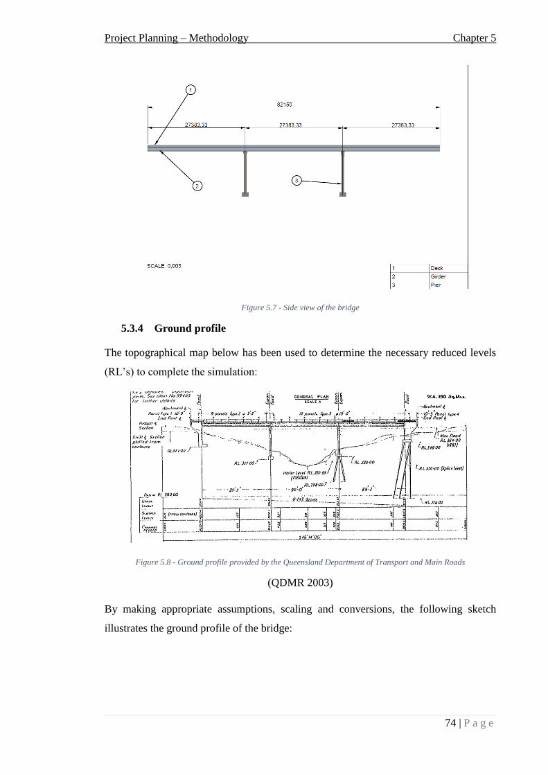
Project Planning – Methodology Chapter 5
74 | P a g e
Figure 5.7 - Side view of the bridge
5.3.4 Ground profile
The topographical map below has been used to determine the necessary reduced levels
(RL’s) to complete the simulation:
Figure 5.8 - Ground profile provided by the Queensland Department of Transport and Main Roads
(QDMR 2003)
By making appropriate assumptions, scaling and conversions, the following sketch
illustrates the ground profile of the bridge:

Project Planning – Methodology Chapter 5
75 | P a g e
Figure 5.9 - Simplified ground profile with appropriate conversions
The following assumptions were made for the above figure:
Both piers are fixed into the ground at the same heights
Assume the difference in height between the two ground levels is negligible,
therefore both piers are fixed into the ground for a height of 2.60 metres from the
base of the footings
5.3.5 Parameters required
The parameters of the channel required for the parametric study are given below. Refer
to appendix C for detailed calculations.
Table 5.1 - Details of channel
According to the department of Transport and Main Roads, the maximum recorded
flooding event (as indicated in figure 5.10) has the following details:
Table 5.2 - Details of maximum flooding event experienced by the bridge

Project Planning – Methodology Chapter 5
76 | P a g e
Now that the 50 year ARI has been determined, the next step was to calculate the
flowrates for the 100 and 500 year ARI. Realistically, as the bridge was almost completely
submerged in the 1887 flooding event, in the event of a 100 or 500 year ARI flood, the
bridge would most likely be completely submerged and hence the channel would begin
overflowing. This would make it extremely difficult to calculate the new cross-sectional
area and hence the velocities could not be determined. Therefore, to determine the
absolute maximum velocities in a 100 and 500 year ARI, it is assumed this will occur
when the bridge is fully submerged, before the channel has begun overflowing. Before
the velocities can be determined, the discharges for these events must be determined. To
obtain these discharges, an annual flood frequency analysis (FFA) was conducted. The
details of this are shown below.
Annual flood frequency analysis
A flood frequency analysis was able to be performed as there was a gauge station
positioned nearby within Tenthill Creek. The Department of Natural Resources and
Mines’ water monitoring portal provided rainfall data for Tenthill Creek from 1968 to
2015, which was a reasonably good range of data. The details of the gauge station are
given below:
Table 5.3 - Site details
(DNRM 2015)
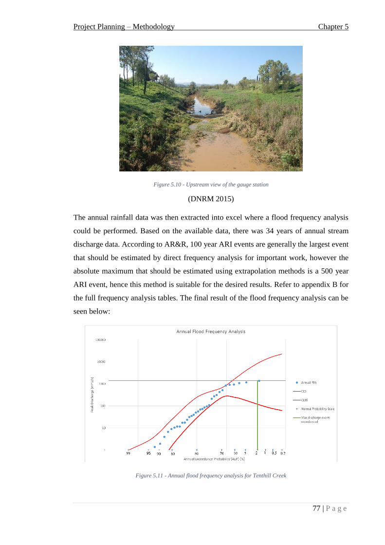
Project Planning – Methodology Chapter 5
77 | P a g e
Figure 5.10 - Upstream view of the gauge station
(DNRM 2015)
The annual rainfall data was then extracted into excel where a flood frequency analysis
could be performed. Based on the available data, there was 34 years of annual stream
discharge data. According to AR&R, 100 year ARI events are generally the largest event
that should be estimated by direct frequency analysis for important work, however the
absolute maximum that should be estimated using extrapolation methods is a 500 year
ARI event, hence this method is suitable for the desired results. Refer to appendix B for
the full frequency analysis tables. The final result of the flood frequency analysis can be
seen below:
Figure 5.11 - Annual flood frequency analysis for Tenthill Creek

Project Planning – Methodology Chapter 5
78 | P a g e
It can be seen in figure 3.14 that the data isn’t of a very high standard to perform “neat”
results, however this was the only data available. To verify that the method was correct,
the maximum discharge that was experienced (the 1887 event) was plotted and the point
was located right in the middle of the confidence limits. A fitted Log-Pearson 3 (LP3)
curve was not sufficient enough to provide an accurate extrapolation of the 100 and 500
year ARI discharges. Therefore, a manual best line of fit was drawn and the values were
drawn off. It was determined that the approximate 100 and 500 year ARI discharges were:
Q (100 year ARI) = 1900 m3/s
Q (500 year ARI) = 2200 m3/s
Now that the discharges for the major and extreme flooding events have been determined,
the velocities can be determined. Since the discharge is dependent on the cross-sectional
area as well as the flow velocity, two velocities were determined for each flooding event,
one velocity was the worst case velocity scenario and the other was the worst case flood
height scenario. The worst case velocity scenario assumes the bridge is fully submerged,
however the flood height does not increase above the top deck level, therefore this gives
the maximum possible velocities for each flooding event. The worst case flood height
velocities give the relevant velocities in the situation that the flood level exceeds the top
level of the deck, therefore the increase in cross-sectional area means that there will be
an associated decrease in the velocities.
Table 5.4 - Summary of velocities and flood heights
3.5.4 Assumptions
The following assumptions were made in the simplification of the bridge:
The railings were neglected. This is due to the fact that the structural integrity of
the entire bridge is being investigated and the railings will have very little effect

Project Planning – Methodology Chapter 5
79 | P a g e
on the failure of a bridge. It should be noted that in reality, the railings could have
an effect on the flow when the flood level exceeds the top level of the deck. Debris
are most likely to get lodged within the railings, which in addition with the railings
themselves, can disturb the flow above the deck level by creating vortices.
However this is outside the scope of this project as CFD modelling would be
required to simulate these effects and the extra time is simply not worth it as the
structural integrity of the entire bridge is the main concern.
The abutments were neglected. The girders are assumed as simply supported so
simple restraints will be applied to the girders in Strand7 to replace the abutments
The steel reinforcement within the concrete has been neglected. This is because it
is very complex to model steel reinforcement of that level within Strand7 and it is
outside the scope of this project
The piles below the footings have been neglected. The footings are assumed to be
completely fixed into the ground so the piles will have no effect during the
simulation process
All other small components of the bridge have been neglected. All other small
components will have minimal effect on the performance of the bridge during a
flooding event, therefore these have been neglected to save time during the
simulation process

Project Planning – Methodology Chapter 5
80 | P a g e
5.4 Simulation Method
As the simulation process will consist of a bridge model with simple hydrodynamic forces
being applied, the simulation of the flood loadings on the identified bridge models will
be performed using the Strand7 software package. Strand7 is a Finite Element Analysis
(FEA) software product developed by Strand 7 Pty. Ltd. Strand7 is most commonly used
for the construction and mechanical engineering sectors, but also has seen use in other
areas of engineering including aeronautical, marine and mining. Strand7 includes solvers
such as linear static, natural frequency, buckling, nonlinear static, linear and nonlinear
transient dynamic, spectral and harmonic response, linear and nonlinear steady-state heat
transfer, linear and nonlinear transient heat transfer (Strand7 2015). As the loading is not
very complicated, the linear static solver will be used throughout this project.
The linear static solver performs the following steps:
Calculates and assembles element stiffness matrices, equivalent element force
vectors and external nodal force vectors. In the stiffness calculation, material
temperature dependency is considered through the user nominated temperature
case. Either consistent or lumped element equivalent load vectors can be
calculated according to the option setting. Constraints are also assembled in
this process.
Solves the equations of equilibrium for the unknown nodal displacements.
Calculates element strains, stresses, stress resultants and strain energy densities
as requested.
(Strand7 2015)

Simulation Chapter 6
81 | P a g e
CHAPTER 6 SIMULATION
6.1 Chapter Overview
The following chapter will present the simulation section of the report. Firstly, a simple
bridge deck model will be analysed in Strand7. The simple bridge deck model was
intended to be a learning exercise for the author, these skills will then be used to model
the Tenthill Creek Bridge, as introduced in chapter 5, section 5.3 of this report. The
purpose of this chapter is to illustrate the development of the bridge models in Strand7.
The Tenthill Creek Bridge model results will then be presented and analysed in chapter
7.
6.2 Simple bridge deck model
6.2.1 Model development
The first simulation was on a very simple model, consisting of a bridge deck with supports
at each end. The geometry of the structure can be seen in figure 6.1:
Figure 6.1 - Cross sectional view of the structure
6.2.2 Simulation parameters
As shown in figure 6.1, the model was divided into three elements for simple and accurate
meshing, the dimensions can be seen in table 6.1:
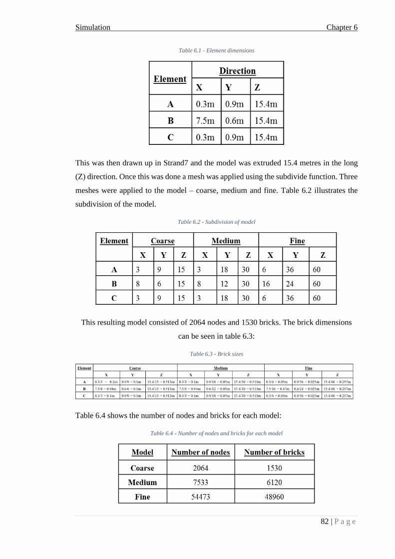
Simulation Chapter 6
82 | P a g e
Table 6.1 - Element dimensions
This was then drawn up in Strand7 and the model was extruded 15.4 metres in the long
(Z) direction. Once this was done a mesh was applied using the subdivide function. Three
meshes were applied to the model – coarse, medium and fine. Table 6.2 illustrates the
subdivision of the model.
Table 6.2 - Subdivision of model
This resulting model consisted of 2064 nodes and 1530 bricks. The brick dimensions
can be seen in table 6.3:
Table 6.3 - Brick sizes
Table 6.4 shows the number of nodes and bricks for each model:
Table 6.4 - Number of nodes and bricks for each model

Simulation Chapter 6
83 | P a g e
It was assumed that the deck was supported in the typical ‘pin and roller’ form, which
can be better illustrated in figure 6.2:
Figure 6.2 - Typical pin and roller support
Using this form, the restraints of the model were defined as:
Table 6.5 - Boundary conditions for the model
The model development using the three different mesh sizes are shown in figures 6.3-6.5:
Figure 6.3 - Coarse simulation model

Simulation Chapter 6
84 | P a g e
Figure 6.4 - Medium simulation model
Figure 6.5 - Fine simulation model
6.2.3 Input parameters
Since it is only a bridge deck being analysed in this situation, the major contributing force
is drag force. The following drag force equation that was extracted from BA 59/94
(section 5.2) will be used:
𝐹𝑑 = 𝐶𝑑𝜌𝑈𝑜
2𝐻
2000
The following parameters have been assumed:
Cd = 2.0
ρ = 1000kg/m3

Simulation Chapter 6
85 | P a g e
Uo = 2-10m/s. Since a case study will not be used for this project, a range has been
chosen. Three velocities will be chosen, these are 3m/s, 6m/s and 9m/s.
H = 3.9m (assuming the deck is situated 3m above the bed floor level + 0.9m deck
height)
f'c = 32MPa
Inputting these variables into the above equation and converting to MPa we get:
𝐹𝑑1 = 0.009 𝑀𝑃𝑎
𝐹𝑑2 = 0.036 𝑀𝑃𝑎
𝐹𝑑3 = 0.081 𝑀𝑃𝑎
6.2.4 Simulation results
The run time for each model can be seen in table 6.6:
Table 6.6 – Run times for the models
The maximum displacements and stresses of the coarse model can be seen in table 6.7:
Table 6.7 - Coarse model results
The maximum displacements and stresses of the medium model can be seen in table 6.8:
Table 6.8 - Medium model results
The maximum displacements and stresses of the fine model can be seen in table 6.9:

Simulation Chapter 6
86 | P a g e
Table 6.9 - Fine model results
The results in tables 6.7-6.9 give an indication of the changes in results between the
different qualities of meshes. The displacement results have very little changes, therefore
the coarse model does an adequate job of predicting the behaviour of the model. The
stress concentration results appear to double in size for each mesh, this is expected
because a smaller mesh size means the same force acting over a smaller area which means
a greater pressure. Since the mesh sizes were being decreased by half the previous amount
each time, this will result in twice the stress concentration.
Figure 6.6 illustrates the displacement of the model set at 5% scale:
Figure 6.6 - Deformed model set a 5% displacement scale
6.2.5 Discussion
The simple bridge model was intended as a learning exercise for the author. The simple
bridge deck model successfully assisted the author in the following ways:
1. Use of the “extrusion” tool in Strand7 to create three dimensional elements. The
process is to essentially create one (or more if needed) cross sections, the extrusion
tool gives the cross-section the required length and hence converts the model from
two dimensional to three dimensional
Simulation Chapter 6
87 | P a g e
2. Application of restraints for three dimensional models. As explained in section
6.1.2 of this chapter, supports vary in the degrees of freedom for two and three
dimensional supports. This is essential to understand and the model will not work
if the proper restraints aren’t assigned.
3. Application of a manual mesh by use of the “subdivide” function. This is another
essential component of setting up a 3D model in Strand7. As shown in section 6.1.4
of this chapter, the results can vary greatly depending on the size of the mesh. If
the mesh is too coarse, the results can be very inaccurate and give misleading
results. On the other hand, a fine model can give much more accurate results,
however the computation time can greatly increase and begin to take many hours.
It all depends on how accurate results are required and how much the results vary
depending on the mesh size. Also, the different shape sizes that make up the model
are a big factor when determining a suitable mesh size. For example, rectangular
blocks do not need a very small mesh size because convergence is not an issue and
the model will not have much difficulty distributing the stress, however rounded
surfaces or sharp edges where stress concentration could be a very big issue
requires a very fine mesh size, or else the model could provide very misleading
results. It is ultimately a judgement call.
Overall, the simple bridge deck model proved to be a very good learning exercise and
made the author much more proficient in performing 3D modelling in Strand7. These
skills could then be applied to a more complex, realistic bridge within the Lockyer Valley.

Simulation Chapter 6
88 | P a g e
6.3 Tenthill Creek Bridge
6.3.1 Creating the geometric model
Using the dimensions from the engineering drawings presented in chapter 3, the
geometric model could be modelled in Strand7. Firstly, nodes were created at specific
cross sections to define the boundary of each element, then tri3 (where appropriate) and
quad4 elements were created, this defined the cross-section for each element, then these
two-dimensional elements were extruded in the relevant direction, thereby creating the
required three-dimensional elements. Different elements had to be extruded in different
directions, depending on the orientation of the cross-sections created. For example, the
superstructures were extruded in the Z-direction because there is no change in shape along
the Z-axis, however this is not the case for the headstocks, and therefore the headstocks
had to be extruded in the X-direction instead. The final geometric model can be seen in
figure 6.7:
Figure 6.7 - Final geometric model
It can be seen in figure 6.7 that there have been different brick properties assigned to each
component of the bridge, this was done to allow each component to be isolated when
needed, which would assist in the load application and meshing of the model. Table 6.10
shows the classification of each different section.

Simulation Chapter 6
89 | P a g e
Table 6.10 - Property types for the model
6.3.2 Material properties
According to the Department of Transport and Main Roads, the entire bridge consists of
concrete with a characteristic strength of 20MPa. The rest of the material properties were
obtained from the Strand7 library. The material properties are presented in table 6.11:
Table 6.11 - Material properties
Where:
E = Modulus of elasticity
ν = Poison’s Ratio
ρ = density
6.3.3 Restraints of the model
The model was restrained in the following manner:
The footings have been modelled as being cast monolithically with the piers.
The piers have been modelled as being cast monolithically with the headstock.

Simulation Chapter 6
90 | P a g e
The deck has been modelled as being cast monolithically with the girders as well
as pinned supports on either end.
The three spans of girders have been assumed to be simply supported.
The freedom conditions can be seen in table 6.12:
Table 6.12 - Degrees of freedom used for each type of support
To model the segments as being monolithically cast, this was done by assigning the
intersecting points of each segments the same node number, thereby creating a rigid joint.
For example, where the top of the girder meets the bottom of the deck, the girders were
first created and then the deck was created using the top nodes at each girder. The main
problem with assigning the restraints was restraining the girders to the headstock. To do
this, links were created between the bottom level of the girders and the top level of the
headstock. To allow this, the headstock had to be created in such a way that there were
nodes situated directly below the bottom level nodes of the girder (a gap of 200mm was
made between the girders and the headstock). The master-slave option was used for this.
The Master-Slave links are used to force nodes to share degrees of freedom.
The degrees of freedom defined in table 6.12 were used. This can be better illustrated in
figure 6.8:
Figure 6.8 - Degrees of freedom for fixed (left), pinned (middle) and roller (right) links
6.3.4 Meshing of the model
An initial mesh of 500mm was chosen to be applied to the model. Since Strand7 doesn’t
have a function that auto-meshes a model built manually in the program, the Subdivide

Simulation Chapter 6
91 | P a g e
function was used. It should be noted that a fine mesh is not required for this model, this
is because we are looking at the overall structural integrity of the structure. It was shown
in in section 6.1.4 of this chapter that the displacement results had very little changes
between the different quality meshes, this is because the structure consisted of simple
rectangular bricks, therefore convergence was not an issue in the solving process; it is a
similar case for this model. Furthermore, due to the size of the model, a fine mesh was
simply not worth the extra run time. The purpose of this simulation is to be able to
compare the results obtained from the different design standards, however when a fine
mesh was applied to the model, the relative increase in accuracy between the results of
each model was the same, therefore the model still produced the same comparative
results. Hence, the 500mm mesh size was deemed feasible for the simulation. The
subdivision of each element of the model can be seen in table 6.13:
Table 6.13 - Model meshing
It should be noted that the tri6 elements could only be subdivided in 2 directions, rather
than 3; that is why “n/a” was placed in the “Z-direction” column. Also, the pier,
headstock, girders and deck was split into a different number of sections based on their
associated dimension. Figures 6.9-6.11 illustrate the different sections of the model used
in table 6.13.

Simulation Chapter 6
92 | P a g e
Figure 6.9 - Deck sections
Figure 6.10 – Girder (left) and pier (right) sections
Figure 6.11 - Headstock sections
The final meshed model is shown in figure 6.12:

Simulation Chapter 6
93 | P a g e
Figure 6.12 - Meshed model

Results and Discussion Chapter 7
94 | P a g e
CHAPTER 7 RESULTS AND DISCUSSION
7.1 Chapter overview
This chapter presents the results for the different Bridge Design Standards around the
world. This was done by using the “Tenthill Creek Bridge” Strand7 model. Displacement
and stress-concentration results were analysed and used to compare The Australian
Bridge Design Standards (AS5100, 2004) to the International Bridge Design Standards.
A full, comprehensive analysis will be conducted on AS5100, then the most critical
flooding event will be used to analyse the International Standards and determine how the
Australian Standards perform in comparison.
7.2 AS5100
7.2.1 Load cases and load combinations
The load cases used for the AS5100 model are shown in table 7.1:
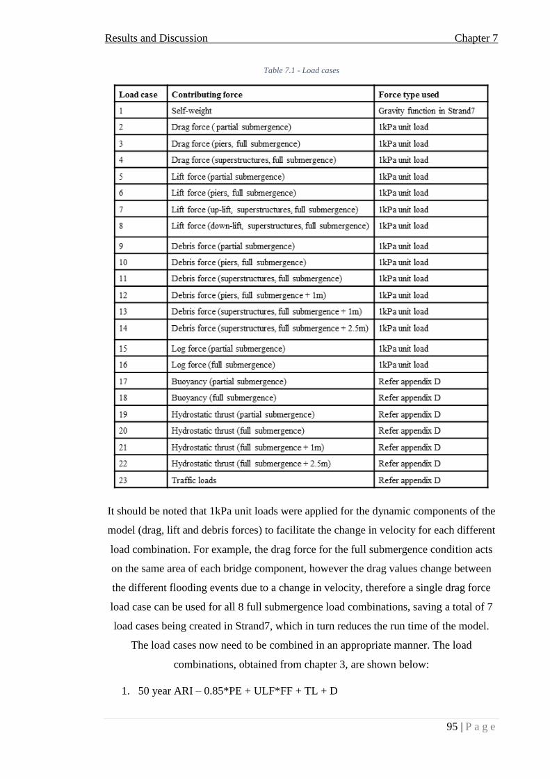
Results and Discussion Chapter 7
95 | P a g e
Table 7.1 - Load cases
It should be noted that 1kPa unit loads were applied for the dynamic components of the
model (drag, lift and debris forces) to facilitate the change in velocity for each different
load combination. For example, the drag force for the full submergence condition acts
on the same area of each bridge component, however the drag values change between
the different flooding events due to a change in velocity, therefore a single drag force
load case can be used for all 8 full submergence load combinations, saving a total of 7
load cases being created in Strand7, which in turn reduces the run time of the model.
The load cases now need to be combined in an appropriate manner. The load
combinations, obtained from chapter 3, are shown below:
1. 50 year ARI – 0.85*PE + ULF*FF + TL + D

Results and Discussion Chapter 7
96 | P a g e
2. 50 year ARI – 0.85*PE + ULF*FF + TL + LI
3. 100 year ARI, worse-case velocity scenario - 0.85*PE + ULF*FF + D
4. 100 year ARI, worse-case velocity scenario – 0.85*PE + ULF*FF + LI
5. 100 year ARI, worse-case flood height scenario - 0.85*PE + ULF*FF + D
6. 100 year ARI, worse-case flood height scenario – 0.85*PE + ULF*FF + LI
7. 500 year ARI, worse-case velocity scenario - 0.85*PE + ULF*FF + D
8. 500 year ARI, worse-case velocity scenario – 0.85*PE + ULF*FF + LI
9. 500 year ARI, worse-case flood height scenario - 0.85*PE + ULF*FF + D
10. 500 year ARI, worse-case flood height scenario – 0.85*PE + ULF*FF + LI
Where:
PE = Permanent effects (self-weight)
ULF = ultimate load factor, as seen in table 7.2:
Table 7.2 - Ultimate load factors
FF = Fluid forces
TL = Traffic loads
D = Debris forces
LI = Log-impact forces
The load combination factors are shown in table 7.3:

Results and Discussion Chapter 7
97 | P a g e
Table 7.3 - Load case factors (AS5100)

Results and Discussion Chapter 7
98 | P a g e
7.2.2 Simulation results
The same type of results as presented in section 6.1.4 of chapter 6 were obtained for this
model, that being X, Y and Z displacement and stress concentration results, with the
addition of resultant XYZ displacement and stress concentration results being obtained.
While the Z, Y and Z displacement and stress concentration results illustrates the
behaviour of the model, it does not take into account “cancelling out” components, hence
that is why XYZ results have also been obtained. The X, Y and Z displacement results
for the AS5100 model are shown in table 7.4 and figure 7.1:
Table 7.4 - X, Y and Z displacement results
These can be better illustrated in figure 7.1:
Figure 7.1 - Bar chart of X, Y and Z displacement results
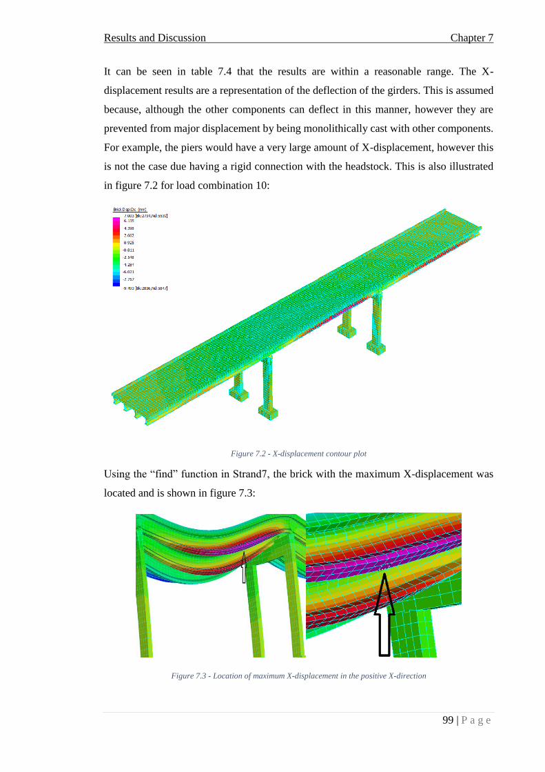
Results and Discussion Chapter 7
99 | P a g e
It can be seen in table 7.4 that the results are within a reasonable range. The X-
displacement results are a representation of the deflection of the girders. This is assumed
because, although the other components can deflect in this manner, however they are
prevented from major displacement by being monolithically cast with other components.
For example, the piers would have a very large amount of X-displacement, however this
is not the case due having a rigid connection with the headstock. This is also illustrated
in figure 7.2 for load combination 10:
Figure 7.2 - X-displacement contour plot
Using the “find” function in Strand7, the brick with the maximum X-displacement was
located and is shown in figure 7.3:
Figure 7.3 - Location of maximum X-displacement in the positive X-direction

Results and Discussion Chapter 7
100 | P a g e
It can be seen that the maximum displacement in the positive X-direction occurred at the
centre, upstream girder, which indicates the maximum point of overturning on the
upstream end of the bridge. Similarly, the maximum X-displacement in the negative X-
direction is located at the left (looking downstream), downstream girder, which indicates
the maximum point of overturning on the downstream end of the bridge.
Figure 7.4 - Location of maximum X-displacement in the negative X-direction
The model was set at 5% displacement scale for figure 7.4 to further illustrate this.
The Y-displacement illustrates the deflection of the deck and the girders. Although the
Headstock can deflect in the Y-direction as well, the size of it stops it from having much
deflection, however the deck is very thin and can therefore deflect much more. This is
shown in figure 7.5:
Figure 7.5 - Y-displacement contour plot

Results and Discussion Chapter 7
101 | P a g e
Again, the find function was used to locate the brick with the maximum Y-displacement.
This is shown in figure 7.6:
Figure 7.6 - Location of maximum Y-displacement
The Z-displacement represents the deflection of the piers and headstock, as well as the
translation of the girders. This is because the deck allows very little displacement in the
Z-direction. This can be seen in figure 7.7:
Figure 7.7 - Z-displacement of the AS5100 model
The location of the brick with the maximum Z-direction was found to be located on the 3
girder (looking downstream), shown in figure 7.8:
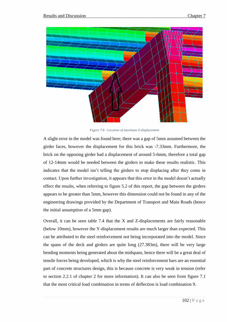
Results and Discussion Chapter 7
102 | P a g e
Figure 7.8 - Location of maximum Z-displacement
A slight error in the model was found here; there was a gap of 5mm assumed between the
girder faces, however the displacement for this brick was -7.33mm. Furthermore, the
brick on the opposing girder had a displacement of around 5-6mm, therefore a total gap
of 12-14mm would be needed between the girders to make these results realistic. This
indicates that the model isn’t telling the girders to stop displacing after they come in
contact. Upon further investigation, it appears that this error in the model doesn’t actually
effect the results, when referring to figure 5.2 of this report, the gap between the girders
appears to be greater than 5mm, however this dimension could not be found in any of the
engineering drawings provided by the Department of Transport and Main Roads (hence
the initial assumption of a 5mm gap).
Overall, it can be seen table 7.4 that the X and Z-displacements are fairly reasonable
(below 10mm), however the Y-displacement results are much larger than expected. This
can be attributed to the steel reinforcement not being incorporated into the model. Since
the spans of the deck and girders are quite long (27.383m), there will be very large
bending moments being generated about the midspans, hence there will be a great deal of
tensile forces being developed, which is why the steel reinforcement bars are an essential
part of concrete structures design, this is because concrete is very weak in tension (refer
to section 2.2.1 of chapter 2 for more information). It can also be seen from figure 7.1
that the most critical load combination in terms of deflection is load combination 9.

Results and Discussion Chapter 7
103 | P a g e
The stress concentration results were also analysed to give an indication of how the
supports behave. The stress concentration results for the AS5100 model are shown in
Table 7.5:
Table 7.5 - X, Y and Z stress concentration results
This is better illustrated in figure 7.9:
Figure 7.9 - Bar chart of X, Y and Z stress concentrations
It can again be seen in table 7.5 that the results are within a reasonable range. Figure 7.9
shows that the Z-stress is by far the most contributing stress. This is because the girders
and deck span in the Z-direction. When the forces are applied to the deck and girders, the
stresses are transferred to the supports, which move in the “Z” direction to get to these
supports. As explained above, the superstructures are much smaller and weaker in

Results and Discussion Chapter 7
104 | P a g e
comparison to the substructures, therefore more stress is generated at the superstructure
supports.
Table 7.6 shows the overall XYZ displacement and stress concentration results.
Table 7.6 - XYZ stress and displacement results
This is better illustrated in figure 7.10:
Figure 7.10 - Bar chart of XYZ stress and displacement results
The “XYZ displacement” shows the overall maximum displacement experienced at a
node in terms of all directions, not just on a single plane. Similarly, the “mean stress”
shows the maximum stress experienced at a brick in any direction, not just a single plane
direction. That is why the values in table 7.6 are smaller than the individual stress
components. This is because, while there is a great deal of stress experienced in the Z-

Results and Discussion Chapter 7
105 | P a g e
direction, some of the X and Y-stresses “cancel out” a portion of the Z-stresses and hence
yields an overall smaller stress concentration result. The above results are a more realistic
representation of the behaviour of the model, therefore these results will be used for the
international bridge design standards and a comparison will be made based off these
results.
7.3 International Design Standards
As shown in section 7.2 of this chapter, the most critical flooding scenario for the bridge
is the 500 year ARI discharge, also the worse-case flood height scenario governs over the
worse-case velocity scenario. Hence, this flooding event was chosen to be used in
comparing the International Bridge Design Standards to the Australian Standards.
7.3.1 BA 59/94
7.3.1.1 Load cases and load combinations
The load cases for the BA59/94 model are shown in table 7.7:
Table 7.7 - Load cases
The load combinations which were used are:
1. G + 1.4*FF + 1.5*D
2. G + 1.4*FF + 1.5*LI
Where:
G = dead loads (self-weight)
FF = fluid forces (drag and lift)
D = Debris forces

Results and Discussion Chapter 7
106 | P a g e
LI = log-impact forces
The corresponding load case factors are shown in table 7.8:
Table 7.8 - Load case factors
7.3.1.2 Simulation results
The displacement results are shown below:
Table 7.9 - X, Y and Z displacement results
The stress concentration results are shown in table 7.10:
Table 7.10 - X, Y and Z stress concentration results
The XYZ stress and displacement results obtained are shown in table 7.11:
Table 7.11 - XYZ stress and displacement results (BA59/94)
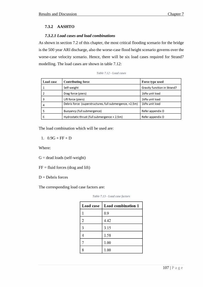
Results and Discussion Chapter 7
107 | P a g e
7.3.2 AASHTO
7.3.2.1 Load cases and load combinations
As shown in section 7.2 of this chapter, the most critical flooding scenario for the bridge
is the 500 year ARI discharge, also the worse-case flood height scenario governs over the
worse-case velocity scenario. Hence, there will be six load cases required for Strand7
modelling. The load cases are shown in table 7.12:
Table 7.12 - Load cases
The load combination which will be used are:
1. 0.9G + FF + D
Where:
G = dead loads (self-weight)
FF = fluid forces (drag and lift)
D = Debris forces
The corresponding load case factors are:
Table 7.13 - Load case factors

Results and Discussion Chapter 7
108 | P a g e
7.3.2.2 Simulation results
The displacement and stress concentration results for the AASHTO model are shown in
tables 7.14 and 7.15, respectively:
Table 7.14 - X, Y and Z displacement results
Table 7.15 - X, Y and Z stress concentration results
The XYZ stress and displacement results obtained can be found in table 7.16:
Table 7.16 - XYZ stress and displacement results
7.3.3 Indian code of practice
7.3.3.1 Load cases and load combinations
As shown in section 7.2 of this chapter, the most critical flooding scenario for the bridge
is the 500 year ARI discharge, also the worse-case flood height scenario governs over the
worse-case velocity scenario. Hence, there will be five load cases required for Strand7
modelling. The load cases are tabulated below:
Table 7.17 - Load cases
There are no load factors that increase or decrease any of the load cases, therefore the
load combination will simply be the sum of the ultimate flood loads.
The corresponding load case factors are:

Results and Discussion Chapter 7
109 | P a g e
Table 7.18 - Load case factors
7.3.3.2 Simulation results
The displacement results are shown below:
Table 7.19 - X, Y and Z displacement results
The stress concentration results are shown below:
Table 7.20 - X, Y and Z stress concentration results
The XYZ stress and displacement results obtained were:
Table 7.21 - XYZ stress and displacement results

Results and Discussion Chapter 7
110 | P a g e
7.4 Comparison of the standards
Now that the results have been obtained, a basic comparative analysis can be performed.
As explained above, the XYZ displacement and mean stress results have been obtained
as they are the best indicator of the behaviour of the bridge, they are also much more
convenient for a comparative analysis. Table 7.22 and figure 7.11 summarises the results
for the most critical flooding scenario:
Table 7.22 - XYZ stress and displacement results for all standards
Figure 7.11 - Bar chart stress and displacement results
The results in table 7.22 indicate that the Australian Standards produce much more severe
results in comparison to the international bridge design standards. These results shows
that the Australian Standards have a higher factor of safety when designing bridges to
resist flooding events. A more detailed comparative analysis is shown below.
The X, Y and Z displacement results for all Design Standards are shown in table 7.23 and
figure 7.12.
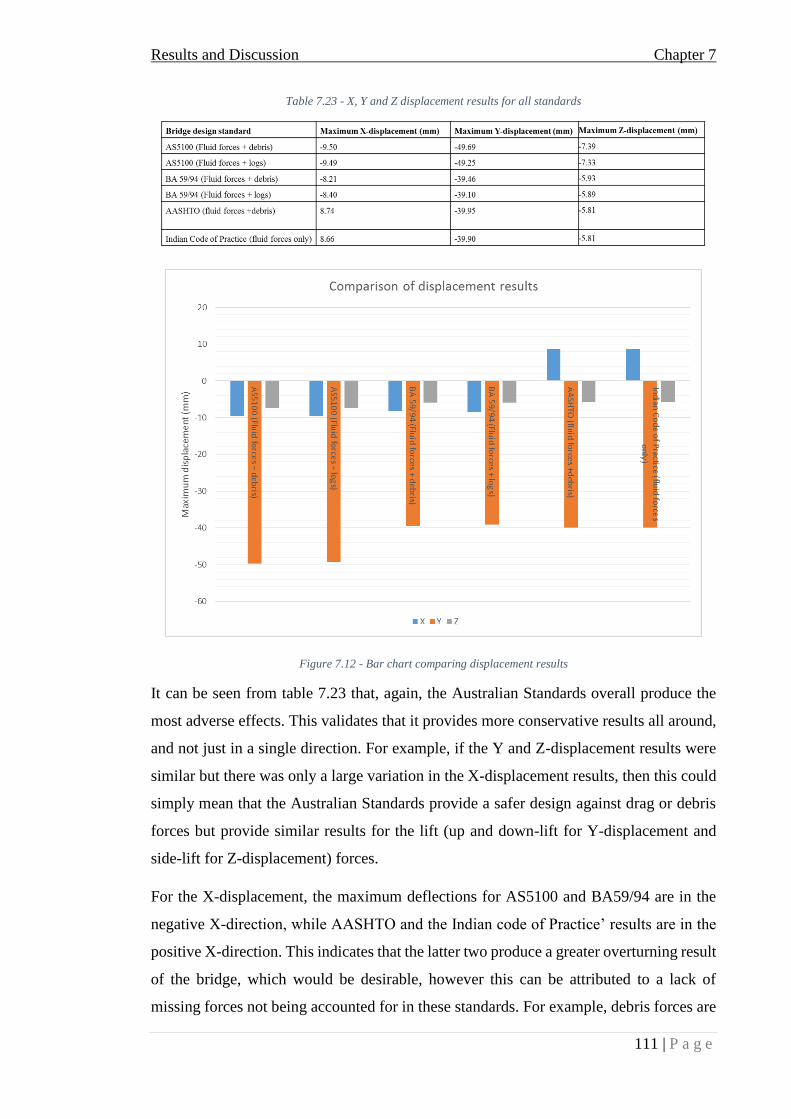
Results and Discussion Chapter 7
111 | P a g e
Table 7.23 - X, Y and Z displacement results for all standards
Figure 7.12 - Bar chart comparing displacement results
It can be seen from table 7.23 that, again, the Australian Standards overall produce the
most adverse effects. This validates that it provides more conservative results all around,
and not just in a single direction. For example, if the Y and Z-displacement results were
similar but there was only a large variation in the X-displacement results, then this could
simply mean that the Australian Standards provide a safer design against drag or debris
forces but provide similar results for the lift (up and down-lift for Y-displacement and
side-lift for Z-displacement) forces.
For the X-displacement, the maximum deflections for AS5100 and BA59/94 are in the
negative X-direction, while AASHTO and the Indian code of Practice’ results are in the
positive X-direction. This indicates that the latter two produce a greater overturning result
of the bridge, which would be desirable, however this can be attributed to a lack of
missing forces not being accounted for in these standards. For example, debris forces are

Results and Discussion Chapter 7
112 | P a g e
not taken into account in the Indian Code of Practice, which would resist overturning of
the structure. Also, downward and up-lift forces aren’t taken into account, which also
increase the resistance to overturning. The Y and Z-displacements are all reasonable and
expected results.
The stress concentration results for all of the standards are shown in table 7.24 and figure
7.13
Table 7.24 - X, Y and Z stress concentration results for all standards
Figure 7.13 - Bar chart of X, Y and Z stress concentration results
The results above again indicate that the Australian Standards produce more adverse
effects overall in terms of stress concentration. To compare each standard to the
Australian Standard, the relative difference between the Australian Standard and the
International Standard of interest was calculated for the most critical load combinations
in X, Y and Z stress-concentration. From this, the average relative change was found to
give an overall indicator of the difference in results.

Results and Discussion Chapter 7
113 | P a g e
Table 7.25 - Relative difference of the International Standards vs Australian Standard
It can be concluded from table 7.25 that, in comparison to the Australian Standards, the
British Standard (BA 59/94) produces the least adverse effect for the 500 year ARI
flooding event. This is then followed by the American Standard and finally the Indian
Code of Practice.
Overall, the results indicate that there is no recommendations that can be made to the
Australian Standards, based on the results produced by the international standards.
International Standard Relative difference in X-stress Relative difference in Y-stress Relative difference in Z-stress Average relative difference
BA 59/94 22.65% 16.58% 22.61% 20.62%
AASHTO 15.73% 28.05% 15.31% 19.70%
Indian Code of Practice 16.19% 26.33% 16.04% 19.52%

Conclusions and Futher Work Chapter 8
114 | P a g e
CHAPTER 8 CONCLUSIONS AND FUTHER
WORK
8.1 Summary
This research project has successfully analysed the behaviour of bridges subjected to
flood loadings based on different design standards from around the world. Flood loadings,
traffic loadings and load combinations were identified from the Australian Bridge Design
Standard, AS5100, 2004. Flood loadings and load combinations were also identified from
an American standard, AASHTO LFRD Bridge Design Specifications, 2012, a European
standard, BA59/94 as well as an Asian standard, Indian code of Practice, 2014. As a
learning process, a simple bridge deck model was simulated in Strand7 with a simple
flood loading applied to it to understand the core skills required. A complex bridge
(Tenthill Creek Bridge) was successfully identified within the Lockyer Valley Region
that is prone to extreme flooding events and data was gathered on the bridges details,
however simplifications had to be made to assist in the simulation. The skills obtained
from the simple bridge deck model were applied successfully to the complex bridge
model. Various submergence conditions were identified and a full, comprehensive
analysis was conducted on AS5100 to determine the most critical loading condition. It
was determined that a flood height scenario gave the most adverse effects in comparison
to the velocity scenarios. The most critical submergence case was identified and this
submergence case was used for the modelling of the bridge subjected to the flood loadings
from international standards. It was determined that AS5100 produced the most adverse
effects in terms of stress concentration and displacement. Based on the results, it was
determined that no recommendations could be made to AS5100, based off the results
produced by the international standards.
8.2 Achievement of Project Objectives
The following project objectives have been addressed:
1) Research literature and background information relating to the different types of
bridges, including the different construction practices used, as well as natural disasters

Conclusions and Futher Work Chapter 8
115 | P a g e
This has been addressed in chapter two of the report. Basic concepts relating to bridges,
bridge construction as well as natural disasters (mainly flooding) have been introduced
and linked together via example events. Also, the basic concepts relating to the different
types of forces have been outlined.
2) Research and compare bridge design standards from around the world and identify
flood loadings and load combinations that need to be taken into consideration for the
design of a bridge in areas prone to flooding
This has been addressed in chapters three and four of this report. Chapter three
successfully identified the flood loadings, traffic loads and load combinations that are
outlined in the standards when designing bridges in flood prone areas. Chapter four
outlines the flood loadings and load combinations recommended within the International
standards. The comparison between the standards was performed in chapter 7.
3) Simulate the behaviour of a small, simple bridge subjected to the identified flood
loadings
This has been addressed in chapter 6, section 6.2 of the report. This section shows the
model development as well as some example results with a simple flood loading applied.
This section was intended as a learning exercise for the author.
4) Identify a more complicated, realistic bridge in the Lockyer Valley Region that is
prone to extreme flooding events and collect available data on the bridge
This has been successfully addressed in section 5.3 of this report. This section gives the
bridge details and flooding parameters required to successfully perform the simulation.
Simplifications were made to the bridge structure to assist in the simulation process as
accurate results were not a number one priority for this simulation.
5) Simulate the behaviour of the bridge subjected to different flood loadings from the
available design standards
This has been addressed in section 6.3 and chapter 7 of the report. Section 6.3 presents
the development process of the model such as the geometric model creation, the model
restraints as well as the meshing of the model. The simulation results were displayed by
means of bar charts and tables and discussed in chapter 7

Conclusions and Futher Work Chapter 8
116 | P a g e
6) Draw appropriate conclusions as to how the Australian Bridge Design Standards
perform in a flooding event in comparison to different standards around the world
This has been addressed in chapter 7 and section 8.1 of this report.
7) Make recommendations for the Australian bridge design standards, AS5100 based on
these results
This has been addressed in section 8.1 of the report. The results from the international
standards did not “out-perform” the Australian Standards in any aspects of the simulation,
therefore specific recommendations could not be made to the Australian Standards based
off the results from the international standards, however general suggestions have been
made in section 8.1.
8.3 Conclusions
In conclusion, it the project aim was successfully achieved. The results indicate that there
were no recommendations that could be made to the Australian Bridge Design Standards
based on the results produced by the International Standards. In fact, the results indicate
that international standards could make a great deal of improvements to their flood
loadings, based on the Australian Standards. Further work would need to be conducted to
determine if specific recommendations could be made to the current Australian Bridge
Design Standards.

117 | P a g e
8.4 Recommendations for future work
As previously mentioned, the model results are very crude, therefore there is a great deal
of future work that can be performed on this project if specific recommendations are to
be made to the Australian Standards. Recommendations for future work are:
1. Prepare a model of Tenthill Creek Bridge that incorporates the steel reinforcement
layers into the structural components of the bridge.
2. Prepare a 3D or Computational Fluid Dynamics (CFD) model of Tenthill Creek
Bridge that accurately describes the behaviour of the fluid during a flooding event.
8.4.1 Incorporation of steel reinforcement
As mentioned in section 3.5.4 of the report, the steel reinforcement has been neglected
from the simulation due to time limitations of the project. As it was shown in chapter 7,
this had a significant effect on the Y-displacement results, giving deflections of almost
50mm. Including steel reinforcement would have a significant improvement on the results
and give a much more accurate indicator of the structural behaviour of the bridge. Due to
the complexity of the steel reinforcement of Tenthill Creek Bridge structural components,
it was simply not an option for this simulation. However, steel reinforcement can be
performed in Strand7 but it is very difficult to model, even for a simple layer of steel
reinforcement. Furthermore, the model would need to be processed by Strand7’s non-
linear analysis solver, which has a very long computational time in comparison to the
linear static solver. Due to the size of the bridge, performing a non-linear analysis in
Strand7 would take extremely long, so a possible option would be to produce a scaled
down model in Strand7. This could make the incorporation of the steel reinforcement
layers even more complicated as they too would need to be scaled down. Furthermore,
the flood loadings would also need to be scaled down.
8.4.2 Accurate modelling of the flow behaviour
Preparing a 3D or CFD model would also have a fairly significant change in the
application of the flood loadings as the current Strand7 model has neglected the water
flow behaviour. For example when the flowing water comes in contact with the pier, the
water will “split” and there will be variable flow distribution around the piers, which will
result in possible “pockets” of stagnant water around the piers as well as vortices being
created by the turbulence. The fluid behaviour will also determine the submergence

118 | P a g e
condition of the bridge. It has been assumed that the water level does not change with
distance along the structure (from the upstream end to the downstream end), which, unless
water was flowing at a very slow velocity, is not the case. Figures 8.1-8.3 show the
different possible submergence conditions for a bridge in the event of a flooding event.
Figure 0.1 - Sluice gate type of pressure flow
Figure 0.2 - Fully submerged pressure flow

119 | P a g e
Figure 0.3 - Pressure and weir flow behaviour

120 | P a g e
(Brunner 2010)
Based on figures 8.1-8.3, for the Tenthill Creek Bridge model, fully submerged pressure
flow has been assumed, however it has been assumed that 𝛼𝑉3
2
2𝑔=
𝛼𝑉22
2𝑔. This has been
assumed to simplify the load application process, however this is not realistic fluid
behaviour. For example, for the full submergence condition where the flood height level
is equal to the top level of the deck, there could be a sluice gate type of pressure flow,
depending on the flow velocity; this could cause air pockets between the girders and
hence there will be no hydrostatic pressure or buoyancy confining the girders, which
could result in more deflection. When the flow velocity is higher, there will be more
flow separation, which could result in the submergence condition changing from fully
submerged pressure flow to sluice gate, which would result in different structural
behaviour by the superstructures.
Finally, if the complex bridge was analysed in a CFD or 3D fluid modelling software
package, the effects of scouring could be taken into account.
If the above recommendations for future work were to be performed then the model
results could be deemed more reliable and further work could then be performed on
investigating finer details and making specific recommendations to the Australian
standards. An example of this could be to make a recommendation to the standards to
change the drag and lift coefficients depending on the submergence conditions (refer
figures 8.1-8.3); there would be a larger down-lift for a fully submerged pressure flow
condition compared to a pressure and weir flow behaviour.

References
121 | P a g e
REFERENCES
Australian Standards 2004, AS 5100.1 - 2004, Bridge Design, Part 1: Scope and General
Principles, Standards Australia, Australia, viewed 09/03/2015,
<http://www.saiglobal.com/PDFTemp/osu-2015-03-09/8267909466/5100.1-
2004(+A1).pdf>.
AASHTO 2012, AASHTO LFRD Bridge Design Specifications, American Association of
State Highway and Transport Officials, viewed 28/06/2015, <
BBC 2009, Body found in Cumbria flood is missing Pc, say police, BBC News, UK,
viewed 16/04/2015, <http://news.bbc.co.uk/2/hi/uk_news/8370865.stm>
BBR 2015, Engineering excellence in bridge construction and heavy lifting, BBR VT
International Ltd, Switzerland, viewed 14/04/2015,
<http://www.bbrnetwork.com/technologies/construction-methods.html>
Blake, M 2013, Longest covered bridge in Asia is destroyed after massive fire ripped
through the 303-metre wooden structure, Associated Newspapers Ltd, viewed
16/04/2015, <http://www.dailymail.co.uk/news/article-2515693/Longest-covered-
bridge-Asia-destroyed-massive-ripped-303-metre-wooden-structure.html>
BOM 2015, FLOODS - Warning, Preparedness & Safety, Australian Government - Berau
of Meteorology, viewed 11/03/2015, <http://www.bom.gov.au/>
Brunner, G 2010, HEC-RAS, River Analysis System Hydraulic Reference Manual, CPD-
69, Hydrologic Engineering Center (HEC), USA,
CivilDigital.com 2015, Bridge Engineering – Components of Bridge Structures,
CivilDigital, viewed 16/04/2015, <http://civildigital.com/bridge-engineering-
components-classification-bridges/>
Congress, IR 2014, Standard Specifications and Code of Practice, Loads and Stresses,
Indian Roads Congress, India, viewed 1/08/15, <
Construction, PC 2015, Very Big Box Girder, viewed 13/04/2015,
<http://www.precastconcreteconstruction.com/32/very-big-box-girder>
Constructor, T 2014, COMPARISON BETWEEN PRESTRESSED CONCRETE, RCC
AND ARCH, The Constructor, viewed 06/03/2015,

References
122 | P a g e
<http://theconstructor.org/others/prestressed-concrete-over-reinforced-concrete-and-
arch/6255/>
Corus 2007, Student guide to steel bridge design, Corus Construction Services &
Development, viewed 06/03/2015, <http://discus.steel-
sci.org/Content/documents/student-guide-steel-bridge-design.pdf>
DNRM 2015, Water monitoring portal, Department of Natural Resources and Mines,
viewed 16/09/2015, <https://www.dnrm.qld.gov.au/water/water-monitoring-and-
data/portal>
efunda 2015, General trapezoid, EFunda, Inc, viewed 21/10/15,
<http://www.efunda.com/math/areas/Trapezoid.cfm>
Friend, C 2013, Concrete Bridge Failures - Deterioration and Spalling, Tangient LLC,
The Pennsylvania State University, viewed 17/04/2015,
<http://failures.wikispaces.com/Concrete+Bridge+Failures+-
+Deterioration+and+Spalling>
Galbraith, R 2009, Living in the Landscape: the Lockyer Valley. A guide to property and
landscape management, South East Queensland Catchments Limited, Brisbane, viewed
13/04/2015,
<http://www.lockyervalley.qld.gov.au/images/PDF/plan_and_build/Environment/living
%20in%20the%20lockyer.pdf>
Government, Q 2015, Fire danger rating, Queensland Government, viewed 15/04/2015,
<https://www.qld.gov.au/emergency/safety/fire-danger.html>
Group, CBD 2015, Types of Concrete Bridges, Concrete Bridge Development Group,
viewed 09/03/2015, <http://www.cbdg.org.uk/intro3.asp>
Hanes, R 2012, prestressed girder box for bridge by Rogers Hanes, viewed 13/04/2015,
<http://www.rogershanes.com/prestress-concrete-girder-box-for-bridge/prestressed-
girder-box-for-bridge-by-rogers-hanes/>
Honert, RCvd & McAneney, J 2011, 'The 2011 Brisbane Floods: Causes, Impacts and
Implications', viewed 09/03/2015, <https://www.riskfrontiers.com/pdf/water-03-
01149.pdf>
Iqbal, S 2013, What is scouring, Bridge Scouring? How to calculate Scour Depth?, Civil
Engineering Blog, viewed 17/04/2015,
<http://www.iamcivilengineer.com/2013/12/what-is-scouring-bridge-scouring-how-
to.html>

References
123 | P a g e
Johnson, P 2015, Bridge Scour and Stream Stability, Department of Civil and
Environmental Engineering, PennState University, viewed 17/04/2015,
<http://www.personal.psu.edu/faculty/p/a/paj6/Research.html>
LaViolette, M, Wipf, T, Lee, Y-S, Bigelow, J & Phares, B 2007, BRIDGE
CONSTRUCTION PRACTICES USING INCREMENTAL LAUNCHING, National
Cooperative Highway Research Progran, Washington D.C, USA,
<http://onlinepubs.trb.org/onlinepubs/archive/NotesDocs/20-07(229)_FR.pdf>
Leeson, D, Fulmer, C & Heron, K 2014, 'Flood Resilient Bridge Design: Case Studies
From Challenging Design Environments', presented at 9th Austroads Bridge Conference,
Sydney, New South Wales, viewed 29/05/15,
<http://www.arrb.com.au/admin/file/content128/c6/11431_CF_Flood%20resilient%20B
ridge%20Design;%20case-
%20studies%20from%20challenging%20design%20environments.pdf>.
Library, LE 2015, Glossary of Bridge Terminology, University of Iowa Libraries, viewed
16/04/2015, <http://sdrc.lib.uiowa.edu/eng/bridges/WaddellGlossary/gloss.htm>
LUSAS 2013, Case Study: Dee River Crossing, viewed 13/04/2015,
<http://www.lusas.com/case/bridge/deeriver.html>
Maeseele, M 2011, Lockyer to face $1b flood bill, The Queensland Times, viewed
13/04/2015, <http://www.qt.com.au/news/ipswich-lockyer-to-face-1b-flood-
bill/758634/>
n.a Lockyer Valley and Toowoomba,
<http://www.floodcommission.qld.gov.au/__data/assets/pdf_file/0004/8788/QFCI-
Interim-Report-Chapter-7-Lockyer-Valley-and-Toowoomba.pdf>
Navy, I 2014, Latest Update on Cyclone Hudhud, Indian Navy, India, viewed 16/04/2015,
<http://www.indiannavy.nic.in/press-release/latest-update-cyclone-hudhud>
NSW, RaTAo 2008, Timber Bridge Manual, 1 edn, Bridge Engineering Technology
Branch Roads and Traffic Authority of NSW, viewed 07/03/2015
<http://www.rms.nsw.gov.au/documents/projects/key-build-
programs/maintenance/tbm-1.pdf>
PERI 2015, Motorway bridge over the Rio Sordo, PERI Group, viewed 5/4/2015,
<http://www.peri.com.kw/projects/projects/civil-engineering-
projects/motorway_bridge_rio_sordo.cfm>
Pritchard, R 2013, 2011 to 2012 Queensland floods and cyclone events:

References
124 | P a g e
Lessons learnt for bridge transport infastructure, Institution of Engineers Australia,
viewed 29/05/15, <http://dx.dol.org/10.7158/S13-009.2013.14.2>
Pujol 2015, Reinforced concrete pre-slab, viewed 13/04/2015,
<http://www.archiexpo.com/prod/pujol/reinforced-concrete-pre-slab-89366-
915540.html>
QDMR 2003, Case Study: Comparison of DMR practices and application of FRP
technology (first draft),
Queensland, TSo 2014, Regional First Home Owner Grant - Map of eligible areas,
Queensland Government, viewed 13/04/2015, <https://www.osr.qld.gov.au/historical-
information/information-bul/fhog-boost/regional-fhog.shtml>
REIDsteel 2015, 50m Span Steel Bridge Construction Project, John REID & Sons Ltd,
England, viewed 14/04/2015, <http://www.steel-
bridges.com/existingbridge6258.html?id=21>
Rohleder, W 2015, Segmental Bridge Technology – Established and Evolving, The State
University of New York, New York, USA, viewed 14/04/2015,
<http://mceer.buffalo.edu/education/bridge_speaker_series/2010-
2011/presentations/Rohleder_presentation.pdf>
Saskatchewan, Uo 2015, Hydrostatic force, College of Arts & Science, Saskatchewan,
viewed 05/09/2015, <http://physics.usask.ca/~chang/course/ep324/lecture/lecture8.pdf>
Seaperch 2015, What is Bouyancy?, Seaperch, viewed 12/08/2015,
<http://www.phillyseaperch.org/uploads/9/1/0/6/9106381/buoyancy_for_ms.pdf>
Skwirk 2015, Bushfires and bushfires in Australia, Skwirk Online Education, viewed
15/04/2015, <http://www.skwirk.com/p-c_s-57_u-479_t-1306_c-5027/qld/sose-
geography/disasters/natural-hazards/bushfires-and-bushfires-in-australia>
Standards, A 2004a, AS 5100.1 - 2004, Bridge Design, Part 1: Scope and General
Principles, Standards Australia, Australia, viewed 09/03/2015,
<http://www.saiglobal.com/PDFTemp/osu-2015-03-09/8267909466/5100.1-
2004(+A1).pdf>
Standards, A 2004b, AS 5100.2 - 2004, Bridge Design, Part 2: Design Loads, Standards
Australia, Australia, viewed 8/05/2015, <http://www.saiglobal.com/PDFTemp/osu-
2015-05-08/3768016978/5100.2-2004(+A1).pdf>
SteelConstruction.info 2015, Steel construction.info, viewed 06/03/2015,
<http://www.steelconstruction.info/Bridges>

References
125 | P a g e
Strand7 2015, Strand7 linear static solver, Strand7 Pty. Ltd., Sydney, Australia, viewed
2/06/15, <http://www.strand7.com/html/linearstatic.htm>
The Highways Agency, TSODD, The Welsh Office, The Department of the Environment
for Northern Ireland 1994, Design Manual for Roads and Bridges The Design of Highway
Bridges for Hydraulic Action, viewed 21/08/15, <
Toolbox, TE 2015, Impact force, The Engineering Toolbox, viewed 02/09/2015,
<http://www.engineeringtoolbox.com/impact-force-d_1780.html>
USQ 2014, CIV3506 - Concrete Structures, Studybook, University of Southern
Queensland, University of Southern Queensland, viewed 06/03/2015
<http://www.usq.edu.au/>
U.S. Department of Transportation 2011, Bridge Preservation Guide, Maintaining a State
of Good Repair Using Cost Effective Investment Strategies, The Federal Highway
Administration, USA, viewed 09/03/2015,
<http://www.fhwa.dot.gov/bridge/preservation/guide/guide.pdf>.

Appendices
126 | P a g e
APPENDICES
Appendix A – Project Specifications

Appendices
127 | P a g e
Appendix B – Flood frequency analysis data for Tenthill
Creek
Streamflow data from 1968 to 2015:
Time and Date Max Discharge (Cumecs) Quality code
1/01/1968 0:00 255
1/01/1969 0:00 255
1/01/1970 0:00 255
1/01/1971 0:00 901.602 9
1/01/1972 0:00 49.552 9
1/01/1973 0:00 255
1/01/1974 0:00 255
1/01/1975 0:00 69.84 9
1/01/1976 0:00 519.112 9
1/01/1977 0:00 73.845 9
1/01/1978 0:00 1.388 9
1/01/1979 0:00 17.657 59
1/01/1980 0:00 0 15
1/01/1981 0:00 311.638 60
1/01/1982 0:00 255
1/01/1983 0:00 255
1/01/1984 0:00 40.007 9
1/01/1985 0:00 23.625 60
1/01/1986 0:00 0.001 15
1/01/1987 0:00 10.503 30
1/01/1988 0:00 432.8 60
1/01/1989 0:00 95.65 60
1/01/1990 0:00 56.304 30
1/01/1991 0:00 846.621 60
1/01/1992 0:00 213 59
1/01/1993 0:00 1.93 59
1/01/1994 0:00 0 10
1/01/1995 0:00 11.687 30
1/01/1996 0:00 936.276 60
1/01/1997 0:00 9.002 30
1/01/1998 0:00 0 10
1/01/1999 0:00 17.37 59
1/01/2000 0:00 0.482 60
1/01/2001 0:00 273.925 60
1/01/2002 0:00 0 10
1/01/2003 0:00 0 10
1/01/2004 0:00 6.71 20

Appendices
128 | P a g e
1/01/2005 0:00 85.42 30
1/01/2006 0:00 0 15
1/01/2007 0:00 11.765 30
1/01/2008 0:00 109.805 30
1/01/2009 0:00 3.992 20
1/01/2010 0:00 1176.461 60
1/01/2011 0:00 1098.644 60
1/01/2012 0:00 31.328 30
1/01/2013 0:00 1359.358 60
1/01/2014 0:00 35.118 30
1/01/2015 0:00 255
The quality code variables are given below:
The details of the flood frequency analysis are given below:
Flood frequency analysis table 1:
Variables:
100 - Stream Water Level (Metres)
140 - Stream Discharge (Cumecs)
Qualities:
9 - CITEC - Normal Reading
10 - Good
15 - Water level below threshold (no flow)
20 - Fair
30 - Poor
59 - CITEC - Derived Height
60 - Estimate
255 - No data exists
Formulas
AEP = (m-0.4)/(n+0.2)
ARI = 1/AEP
Mean (M) = ƩX/N
Standard Deviation (S) = [Ʃ(X-M)^2/(N-1)]^0.5
Skew (G) = ((N*Ʃ(X-M)^3)/((N-1)(N-2)*S^3)
Log(Q_Y) = M + Ky*S
Q_Y = 10^Log(Q_Y)
Log(CL5) = Log(Q_Y) + 1.645*(δ*S/sqrt(N))
CL5 = 10^Log(CL5)
Log(CL95) = Log(Q_Y) - 1.645*(δ*S/sqrt(N))
CL95 = 10^Log(CL95)
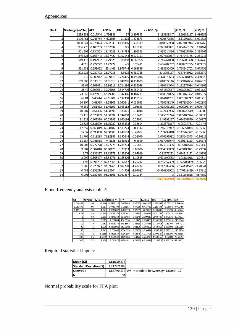
Appendices
129 | P a g e
Flood frequency analysis table 2:
Required statistical inputs:
Normal probability scale for FFA plot:
Rank Discharge (m^3/s) AEP AEP % ARI Z X = LOG(Q) (X-M)^2 (X-M)^3
1 1359.358 0.017544 1.754386 57 2.107345 3.133333847 2.29931117 3.486556
2 1176.461 0.046784 4.678363 21.375 1.676873 3.070577535 2.11292871 3.071336
3 1098.644 0.076023 7.602339 13.15385 1.432339 3.040856988 2.027408944 2.886769
4 936.276 0.105263 10.52632 9.5 1.25212 2.971403891 1.834448159 2.48461
5 901.602 0.134503 13.45029 7.434783 1.105355 2.955014866 1.790321579 2.395502
6 846.621 0.163743 16.37427 6.107143 0.979191 2.927689037 1.717942775 2.251713
7 519.112 0.192982 19.29825 5.181818 0.866958 2.715261068 1.206208398 1.324749
8 432.8 0.222222 22.22222 4.5 0.76471 2.636287252 1.038975295 1.059029
9 311.638 0.251462 25.1462 3.976744 0.669896 2.493650409 0.768540702 0.673752
10 273.925 0.280702 28.07018 3.5625 0.580758 2.43763167 0.67345952 0.552672
11 213 0.309942 30.99415 3.226415 0.496016 2.328379603 0.506081035 0.360023
12 109.805 0.339181 33.91813 2.948276 0.414699 2.040622116 0.179467664 0.076029
13 95.65 0.368421 36.84211 2.714286 0.336038 1.980684974 0.132277034 0.048109
14 85.42 0.397661 39.76608 2.514706 0.259406 1.931559567 0.098956607 0.031129
15 73.845 0.426901 42.69006 2.342466 0.184271 1.868321095 0.063169392 0.015877
16 69.84 0.45614 45.61404 2.192308 0.110162 1.844104231 0.051582747 0.011715
17 56.304 0.48538 48.53801 2.060241 0.036655 1.750539249 0.017836504 0.002382
18 49.552 0.51462 51.46199 1.943182 -0.03665 1.695061188 0.006095754 0.000476
19 40.007 0.54386 54.38596 1.83871 -0.11016 1.602135986 0.000220519 -3.3E-06
20 35.118 0.573099 57.30994 1.744898 -0.18427 1.545529774 0.005105974 -0.00036
21 31.328 0.602339 60.23392 1.660194 -0.25941 1.49593267 0.014653879 -0.00177
22 23.625 0.631579 63.15789 1.583333 -0.33604 1.373371817 0.05934781 -0.01446
23 17.657 0.660819 66.08187 1.513274 -0.4147 1.246916917 0.136951034 -0.05068
24 17.37 0.690058 69.00585 1.449153 -0.49602 1.239799818 0.142269322 -0.05366
25 11.765 0.719298 71.92982 1.390244 -0.58076 1.070591932 0.298546343 -0.16312
26 11.687 0.748538 74.8538 1.335938 -0.6699 1.067703044 0.30171163 -0.16573
27 10.503 0.777778 77.77778 1.285714 -0.76471 1.021313365 0.35482574 -0.21136
28 9.002 0.807018 80.70175 1.23913 -0.86696 0.954339009 0.439100871 -0.29097
29 6.71 0.836257 83.62573 1.195804 -0.97919 0.82672252 0.624516172 -0.49353
30 3.992 0.865497 86.54971 1.155405 -1.10535 0.601190533 1.03184018 -1.04814
31 1.93 0.894737 89.47368 1.117647 -1.25212 0.285557309 1.772702029 -2.36023
32 1.388 0.923977 92.39766 1.082278 -1.43234 0.142389466 2.174434572 -3.20641
33 0.482 0.953216 95.32164 1.04908 -1.67687 -0.316952962 3.740119429 -7.23316
34 0.001 0.982456 98.24561 1.017857 -2.10734 -3 21.31655858 -98.4182
54.97751979 48.93791607 -92.9794
ARI AEP (%) Ky (G=-0.3) LOG(Q_Y) Q_Y δ Log CL5 CL5 Log CL95 CL95
1.010101 99 -3.416 -2.5429212 0.002865 7.37095 -0.01062 0.975847 -5.07522 8.41E-06
1.052632 95 -1.967 -0.7783704 0.166583 3.49915 0.423769 2.653193 -1.98051 0.010459
1.111111 90 -1.327 0.0010032 1.002313 2.32555 0.79995 6.308848 -0.79794 0.159242
1.25 80 -0.668 0.8035146 6.360842 1.73395 1.399216 25.07357 0.207813 1.613663
2 50 0.261 1.9348242 86.06453 1.35145 2.399117 250.6786 1.470531 29.54821
5 20 0.813 2.607034 404.6076 0.6445 2.828453 673.6792 2.385615 243.0048
10 10 0.982 2.8128374 649.8863 1.22595 3.234015 1714.015 2.39166 246.411
20 5 1.075 2.9260901 843.5098 1.94175 3.593182 3919.059 2.258998 181.5509
50 2 1.141 3.006463 1014.993 2.70105 3.934414 8598.32 2.078512 119.8154
100 1 1.1685 3.0399517 1096.356 3.12545 4.113706 12992.89 1.966198 92.51195
200 0.5 1.1855 3.0606539 1149.884 3.4422 4.243228 17507.65 1.87808 75.52312
500 0.2 1.198 3.075876 1190.902 3.73365 4.358578 22833.8 1.793174 62.11177
Mean (M) 1.616985876
Standard Deviation (S) 1.217771388
Skew (G) -1.657694572 <== interpolate between g=-1.6 and -1.7
N 34

Appendices
130 | P a g e
Y Z-value Y-zero
99 -2.3263479 1
95 -1.6448536 1
90 -1.2815516 1
80 -0.8416212 1
50 0 1
20 0.8416212 1
10 1.2815516 1
5 1.6448536 1
2 2.0537489 1
1 2.3263479 1
0.5 2.5758293 1
0.2 2.8781617 1
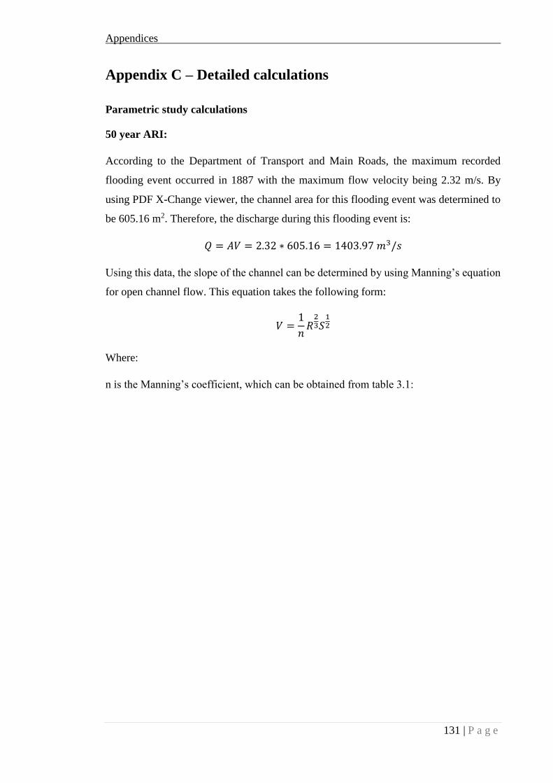
Appendices
131 | P a g e
Appendix C – Detailed calculations
Parametric study calculations
50 year ARI:
According to the Department of Transport and Main Roads, the maximum recorded
flooding event occurred in 1887 with the maximum flow velocity being 2.32 m/s. By
using PDF X-Change viewer, the channel area for this flooding event was determined to
be 605.16 m2. Therefore, the discharge during this flooding event is:
𝑄 = 𝐴𝑉 = 2.32 ∗ 605.16 = 1403.97 𝑚3/𝑠
Using this data, the slope of the channel can be determined by using Manning’s equation
for open channel flow. This equation takes the following form:
𝑉 =1
𝑛𝑅
23𝑆
12
Where:
n is the Manning’s coefficient, which can be obtained from table 3.1:

Appendices
132 | P a g e
(Toolbox 2015)
Based on the images of the channel above, it can be seen that the channel can be classified
as “Earth channel – weedy”, which yields a Manning’s coefficient, n = 0.03
S is the slope of the channel
R is the hydraulic radius, which is given by the equation:
𝑅 =𝐴
𝑃

Appendices
133 | P a g e
Where:
A = wetted area. For the maximum flooding event, A = 605.16m2
P = wetted perimeter. By using the “perimeter” tool in PDF X-change viewer, P =
293.54m
Therefore, the hydraulic radius is:
𝑅 =𝐴
𝑃=
605.16
293.54= 2.0616𝑚
Now, using the above equation, the approximate slope of the channel can be determined
by working backwards. Rearranging for the slope and solving, the equation for the slope
of a channel is:
𝑆 = (𝑉𝑁𝑅32)
2
= (2.32 ∗ 0.03 ∗ 2.061632)
2
= 0.042445 = 4.2445% 𝑔𝑟𝑎𝑑𝑒
By looking at the RL’s in figure 3.12, it can be seen that the bed level is situated at
approximately 15.3 metres below the soffit level of the girders. An estimate for the
channel cross-sectional area can be made. By importing the ground profile into PDF X-
change viewer and using the “area” measuring tool, the approximate area was found to
be:
𝐶ℎ𝑎𝑛𝑛𝑒𝑙 𝑎𝑟𝑒𝑎 = 670.41𝑚2
Now the maximum velocities for the corresponding ARI’s can be determined.
𝑀𝑎𝑥 𝑉 (𝐴𝑅𝐼 100) =1900
670.41= 2.834 𝑚/𝑠
𝑀𝑎𝑥 𝑉 (𝐴𝑅𝐼 500) =2300
670.41= 3.282 𝑚/𝑠
Therefore, assuming the 50 year ARI velocity as the minimum velocity, the velocity
ranges for each ARI is:
𝑉 (𝐴𝑅𝐼 50) = 2.32 𝑚/𝑠
𝑉 (𝐴𝑅𝐼 100) = 2.32 − 2.834 𝑚/𝑠
𝑉 (𝐴𝑅𝐼 500) = 2.32 − 3.43 𝑚/𝑠

Appendices
134 | P a g e
Now that the velocity ranges have been determined, the only parameter that is left to
determine is the flood depths. The assumed flood depths for the simulation are given
below:
Realistically, the increased water level will increase the cross-sectional area and will
decrease the velocity as a result to produce the same discharge. Assuming the width of
the section above the bridge deck is constant, new velocities can be calculated. This is
shown below:
𝑁𝑒𝑤 𝑉 (100 𝑦𝑒𝑎𝑟 𝐴𝑅𝐼) =1900
670.41 + (1 ∗ 82.15)= 2.525 𝑚/𝑠
𝑁𝑒𝑤 𝑉 (500 𝑦𝑒𝑎𝑟 𝐴𝑅𝐼) =2200
670.41 + (2.5 ∗ 82.15)= 2.512 𝑚/𝑠
AS5100 load calculations
Full submergence
Drag force
Worst-case velocity scenarios
Pier
𝐹𝑑𝑢 = 0.5 ∗ 𝐶𝑑 ∗ 𝑉𝑢2 ∗ 𝐴𝑑
Cd = 1.4
V50 = 2.32m/s
V100 = 2.834m/s
V500 = 3.43m/s
(pier) Ad1 = 685*(9820+1219-3370) *10^-6 = 5.25m^2
(headstock, full submergence) Ad2 = ((1067+685)/2*1676)*10^-6 = 1.47m^2
(headstock, partial submergence) Ad3 = ((887.85+685)/2)*890*10^-6 = 0.70m^2
Therefore, the drag forces are:
AEP Drag force (kN) Drag Pressure (kPa)
1 in 50 (Ad1) 19.78 3.77

Appendices
135 | P a g e
1 in 50 (Ad3) 2.64
1 in 100 (Ad1) 29.52 5.62
1 in 100 (Ad2) 8.26
1 in 500 (Ad1) 43.24 8.24
1 in 500 (Ad2) 12.11
Superstructures
𝐹𝑑𝑢 = 0.5 ∗ 𝐶𝑑 ∗ 𝑉𝑢2 ∗ 𝐴𝑑
Relative submergence, 𝑆𝑟 = 𝑑𝑤𝑔𝑠
𝑑𝑠𝑝
Proximity ratio, 𝑃𝑟 = 𝑦𝑔𝑠
𝑑𝑠𝑠
Sr = 1857/1857 = 1.00
Pr = (114.207-97.08)*1000/1857 = 9.22
So, Cd = 1.3
V100 = 2.834m/s
V500 = 3.43m/s
Ad = ((1372+485)*82150)*10^-6 = 152.55m^2
𝐹𝑑𝑢100 = 0.5 ∗ 1.3 ∗ 2.8342 = 5.22 𝑘𝑃𝑎
𝐹𝑑𝑢500 = 0.5 ∗ 1.3 ∗ 3.432 ∗ 152.55 = 7.65 𝑘𝑃𝑎
Worst-case flood height scenarios
Pier
𝐹𝑑𝑢 = 0.5 ∗ 𝐶𝑑 ∗ 𝑉𝑢2 ∗ 𝐴𝑑
Cd = 1.4
V100 = 2.525m/s
V500 = 2.512m/s
(pier) Ad1 = 685*(9820+1219-3370) *10^-6 = 5.25m^2
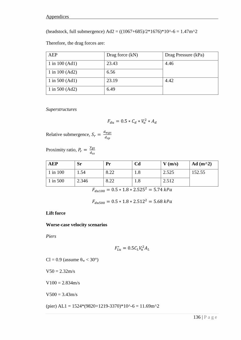
Appendices
136 | P a g e
(headstock, full submergence) Ad2 = ((1067+685)/2*1676)*10^-6 = 1.47m^2
Therefore, the drag forces are:
AEP Drag force (kN) Drag Pressure (kPa)
1 in 100 (Ad1) 23.43 4.46
1 in 100 (Ad2) 6.56
1 in 500 (Ad1) 23.19 4.42
1 in 500 (Ad2) 6.49
Superstructures
𝐹𝑑𝑢 = 0.5 ∗ 𝐶𝑑 ∗ 𝑉𝑢2 ∗ 𝐴𝑑
Relative submergence, 𝑆𝑟 = 𝑑𝑤𝑔𝑠
𝑑𝑠𝑝
Proximity ratio, 𝑃𝑟 = 𝑦𝑔𝑠
𝑑𝑠𝑠
AEP Sr Pr Cd V (m/s) Ad (m^2)
1 in 100 1.54 8.22 1.8 2.525 152.55
1 in 500 2.346 8.22 1.8 2.512
𝐹𝑑𝑢100 = 0.5 ∗ 1.8 ∗ 2.5252 = 5.74 𝑘𝑃𝑎
𝐹𝑑𝑢500 = 0.5 ∗ 1.8 ∗ 2.5122 = 5.68 𝑘𝑃𝑎
Lift force
Worse-case velocity scenarios
Piers
𝐹𝐿𝑢∗ = 0.5𝐶𝐿𝑉𝑢
2𝐴𝐿
Cl = 0.9 (assume θw < 30°)
V50 = 2.32m/s
V100 = 2.834m/s
V500 = 3.43m/s
(pier) AL1 = 1524*(9820+1219-3370)*10^-6 = 11.69m^2

Appendices
137 | P a g e
(headstock, partial submergence) AL2 = 790*9000*10^-6 = 7.11m^2
(headstock, full submergence) AL3 = 1676*9000*10^-6 = 15.084m^2
Therefore, the lift forces are:
AEP Drag force (kN) Drag Pressure (kPa)
1 in 50 (AL1) 28.31 2.42
1 in 50 (AL2) 17.22
1 in 100 (AL1) 42.25 3.61
1 in 100 (AL3) 54.52
1 in 500 (AL1) 61.89 5.29
1 in 500 (AL3) 79.86
Superstructures
𝐹𝐿𝑢∗ = 0.5𝐶𝐿𝑉𝑢
2𝐴𝐿
Sr = 1,
CL = -2,0.1
V100 = 2.834m/s
V500 = 3.43m/s
For downward lift force:
CL = -2
AL = (9210-2*(305))*82150*10^-6 = 706.49m^2
𝐹𝐿𝑢100∗ = 0.5 ∗ −2 ∗ 2.8342 = −8.03 𝑘𝑃𝑎
𝐹𝐿𝑢500∗ = 0.5 ∗ −2 ∗ 3.432 = −11.76 𝑘𝑃𝑎
For upward lift force:
CL = 0.1
(girder) AL1 = 635*27383.33*10^-6 = 17.39m^2
(deck, outside) AL2 = 400.5*82150*10^-6 = 32.9m^2

Appendices
138 | P a g e
Therefore, the lift forces are:
AEP Drag force (kN) Drag Pressure (kPa)
1 in 100 (AL1) 6.98 0.40
1 in 100 (AL2) 13.21
1 in 500 (AL1) 10.23 0.59
1 in 500 (AL2) 19.35
Worse-case flood height scenarios
Piers
𝐹𝐿𝑢∗ = 0.5𝐶𝐿𝑉𝑢
2𝐴𝐿
Cl = 0.9 (assume θw < 30°)
V100 = 2.525m/s
V500 = 2.512m/s
(pier) AL1 = 1524*(9820+1219-3370)*10^-6 = 11.69m^2
(headstock, full submergence) AL3 = 1676*9000*10^-6 = 15.084m^2
Therefore, the lift forces are:
AEP Drag force (kN) Drag Pressure (kPa)
1 in 100 (AL1) 33.54 2.87
1 in 100 (AL3) 43.28
1 in 500 (AL1) 33.19 2.84
1 in 500 (AL3) 42.83
Superstructures
𝐹𝐿𝑢∗ = 0.5𝐶𝐿𝑉𝑢
2𝐴𝐿
AEP Sr CL
1 in 100 1.54 -2,0.1
1 in 500 2.346 -1.3,0

Appendices
139 | P a g e
V100 = 2.525m/s
V500 = 2.512m/s
For downward lift force:
CL100 = -2
CL500 = -1.3
(Deck, middle) AL1 = (9210-2*(305))*82150*10^-6 = 706.49m^2
(Deck, outside) AL2 = 305*82150*10^-6 = 25.06m^2
AEP Lift force (kN) Lift Pressure (kPa)
1 in 100 (AL1) -4504.32 6.38
1 in 100 (AL2) -159.77
1 in 500 (AL1) -2897.73 4.10
1 in 500 (AL2) -102.79
For upward lift force:
CL = 0.1
(girder) AL1 = 635*27383.33*10^-6 = 17.39m^2
(deck, outside) AL2 = 400.5*82150*10^-6 = 32.9m^2
Therefore, the lift forces are:
AEP Lift force (kN) Lift Pressure (kPa)
1 in 100 (AL1) 5.54 0.32
1 in 100 (AL2) 10.49
Debris force
Worse-case velocity scenario
Pier
𝐹𝑑𝑢∗ = 0.5𝐶𝑑𝑉𝑢
2𝐴𝑑𝑒𝑏

Appendices
140 | P a g e
Vu50^2*y = 2.32^2*(111.56-97.08) = 77.94
Cd1 = 2.45
Vu100^2*y = 2.834^2*(114.207-97.08) = 97.34
Cd2 = 2.2
Vu500^2*y = 3.43^2*(114.207-97.08) = 201.50
Cd3 = 1.7
Adeb = 3*20 = 60m^2 (maximum usable dimensions)
𝐹𝑑𝑢50∗ = 0.5 ∗ 2.45 ∗ 2.322 = 6.59 𝑘𝑃𝑎
𝐹𝑑𝑢100∗ = 0.5 ∗ 2.2 ∗ 2.8342 = 9.84 𝑘𝑃𝑎
𝐹𝑑𝑢500∗ = 0.5 ∗ 1.7 ∗ 3.432 = 14.41 𝑘𝑃𝑎
Superstructures
𝐹𝑑𝑢∗ = 0.5𝐶𝑑𝑉𝑢
2𝐴𝑑𝑒𝑏
Pr = 8.22
F100 = 2.834/(9.81*(114.207-97.08)) = 0.22
Cd100 = 1.8
F500 = 3.43/(9.81*(114.207-97.08)) = 0.26
Cd500 = 1.65
Adeb = 60m^2
𝐹𝑑𝑢100∗ = 0.5 ∗ 1.8 ∗ 2.8342 = 7.23 𝑘𝑃𝑎
𝐹𝑑𝑢500∗ = 0.5 ∗ 1.65 ∗ 3.432 = 9.71 𝑘𝑃𝑎
Worse-case flood height scenario
Pier
𝐹𝑑𝑢∗ = 0.5𝐶𝑑𝑉𝑢
2𝐴𝑑𝑒𝑏

Appendices
141 | P a g e
Vu100^2*y = 2.525^2*(115.207-97.08) = 97.34
Cd2 = 2.1
Vu500^2*y = 2.512^2*(116.707-97.08) = 201.50
Cd3 = 2.05
Adeb = 3*20 = 60m^2 (maximum usable dimensions)
𝐹𝑑𝑢100∗ = 0.5 ∗ 2.1 ∗ 2.5252 = 6.69 𝑘𝑃𝑎
𝐹𝑑𝑢500∗ = 0.5 ∗ 2.05 ∗ 2.5122 = 6.47 𝑘𝑃𝑎
Superstructures
𝐹𝑑𝑢∗ = 0.5𝐶𝑑𝑉𝑢
2𝐴𝑑𝑒𝑏
Pr = 8.22
F100 = 2.525/(9.81*(115.207-97.08)) = 0.2
Cd100 = 1.9
F500 = 2.512/(9.81*(116.707-97.08)) = 0.2
Cd500 = 1.9
Adeb = 60m^2
𝐹𝑑𝑢100∗ = 0.5 ∗ 1.9 ∗ 2.5252 = 6.057𝑘𝑃𝑎
𝐹𝑑𝑢500∗ = 0.5 ∗ 1.9 ∗ 2.5122 = 6.0𝑘𝑃𝑎
Log forces
𝐹𝐿𝑢∗ =
0.5𝑚𝑉𝑢2
𝑠
Assume log has a minimum mass, m = 2000kg.
Stopping distance, s = 75mm
Worse-case velocity scenarios
The channel is very wide, so assume it can hold 3 logs of this size. Apply 1 log force at
each pier and another at the middle girder.

Appendices
142 | P a g e
𝐹𝐿𝑢50∗ =
0.5 ∗ 2000 ∗ 2.322
0.075=
71.765 𝑘𝑁
0.3848𝑚2= 186.50 𝑘𝑃𝑎
For 100 and 500 year ARI, apply
𝐹𝐿𝑢100∗ =
0.5 ∗ 2000 ∗ 2.8342
0.075=
107.09 𝑘𝑁
0.3848𝑚2= 278.30 𝑘𝑃𝑎
𝐹𝐿𝑢500∗ =
0.5 ∗ 2000 ∗ 3.432
0.075=
156.865 𝑘𝑁
0.3848𝑚2= 407.65 𝑘𝑃𝑎
Worse-case flood height scenarios
𝐹𝐿𝑢100∗ =
0.5 ∗ 2000 ∗ 2.5252
0.075=
85.008 𝑘𝑁
0.3848𝑚2= 220.91 𝑘𝑃𝑎
𝐹𝐿𝑢500∗ =
0.5 ∗ 2000 ∗ 2.5122
0.075=
84.135 𝑘𝑁
0.3848𝑚2= 218.65 𝑘𝑃𝑎
Buoyancy
Headstock
Partially submerged:
Fb = ρgV = 1000*9.81*6.23 = 61.80kN/6.165 = 10.02kPa
Fully submerged:
Fb = ρgV = 1000*9.81*(1.676*9*(1.067+0.685)/2) = 129.63kN/6.165 = 21.027kPa
Girders
Fb = ρgV =
1000*9.81*27.383*(0.483*0.152+0.635*0.24+0.635*0.152+(0.483+0.152)/2*0.165+(0.
635+0.152)/22*0.18) = 119.69kN/17.39 = 6.88kPa for each girder
Deck
Fb = ρgV = 1000*9.81*82.15*(0.305*0.485*2+8.6*0.18) = 1485.94kN/756.6 =
1.964kPa
First segment is between edge of the deck and the closest edge of the girders
Second segment is between the girders

Appendices
143 | P a g e
Hydrostatic thrust
For partial submergence, using excel:
Flood level = 11877mm
For the piers:
Where:
y = vertical centroid location from the origin point
h = flood level – y
Therefore, using P = ρgh, the pressures for each element could be calculated.
The
same method was used for the headstocks as well, however the elements are trapezoidal,
and therefore the centroid was calculated using the following formula:
Where the dimensions were as follows:

Appendices
144 | P a g e
(efunda 2015)
The same method has been used for the other submergence conditions, as shown below.
For full submergence:
Flood level = 14772mm
For the piers:
For the headstocks:
For
the girders:

Appendices
145 | P a g e
For
the deck:
For full submergence + 1m:
Flood level = 15772
For the piers:
For
the headstocks:

Appendices
146 | P a g e
For
the girders:
For
the deck:
Also, there will be water pressure on the top of the deck from the extra water. This will
create a uniform pressure distribution of ρgh = 9.81*1 = 9.81kPa in the negative Y
direction.
For full submergence + 2.5m:
Flood level = 17272mm
For the piers:

Appendices
147 | P a g e
For the headstocks:
For the girders:

Appendices
148 | P a g e
For
the deck:
Also, there will be water pressure on the top of the deck from the extra water. This will
create a uniform pressure distribution of ρgh = 9.81*2.5 = 24.525kPa in the negative Y
direction.
Overall, this method of calculating the hydrostatic pressure is not 100% accurate as it is
not accounting for the triangular pressure distribution on top of each of these rectangular
pressure prisms, however, since the difference in height levels is below 500mm, the
pressure difference would be quite small and it can be assumed that it will have a
negligible effect, therefore it is an accurate method for this instance.

Appendices
149 | P a g e
Partial submergence
In the event of partial submergence, traffic loads must be taken into account.
The most likely and most critical traffic scenario is the “M1600 moving traffic load”,
provided in clause 6.2.3 of AS5100.
The M1600 moving traffic load accounts for the loads applied by a moving stream of
traffic. The load is assumed to act within a standard design lane with a width of 3.2m, as
shown in the figure below:
(Standards 2004b)
As shown in the figure above, the applied traffic loads can be taken as a 360kN load
acting over an area of 2.5m x 2m, as well as a line load of 6kN/m acting through the centre
of the lane. For Tenthill Bridge, there are 2 standard design lanes, therefore table 6.6 shall
be taken into account.
(Standards 2004b)
It is more likely that one lane will be loaded, rather than both lanes being loaded
simultaneously. Furthermore, the most critical effect that the traffic loading will have on
the bridge is when the downstream end is loaded (which will contribute to overturning),
hence only the downstream lane will be loaded for the simulation.

Appendices
150 | P a g e
Following clause 6.7, a dynamic load allowance shall be taken into consideration to
account for the interaction between moving vehicles and the bridge structure. The
dynamic load allowance can be obtained from table 6.7.2, as seen below:
(Standards 2004b)
As the M1600 load is the only load being taken into account, α = 0.3, hence:
𝑀1600 𝑙𝑜𝑎𝑑 = (1 + 𝛼) ∗ 𝑙𝑜𝑎𝑑 𝑓𝑎𝑐𝑡𝑜𝑟 ∗ 𝑎𝑐𝑡𝑖𝑜𝑛 𝑢𝑛𝑑𝑒𝑟 𝑐𝑜𝑛𝑠𝑖𝑑𝑒𝑟𝑎𝑡𝑖𝑜𝑛
Where:
Load factor = 1.0
Hence,
𝑇𝑜𝑡𝑎𝑙 𝑡𝑟𝑎𝑓𝑓𝑖𝑐 𝑙𝑜𝑎𝑑 = 1.3 ∗ 𝑀1600 𝑙𝑜𝑎𝑑

Appendices
151 | P a g e
BA59/94 load calculations
Drag force on piers:
𝐹𝐷 = 𝐶𝐷𝜌𝑈𝑜
2
2000
Where:
Uo = 2.512m/s
ρ = 1000kg/m^3
CD = 0.4
𝐹𝐷 = 0.4 ∗ 1000 ∗ 2.5122
2000= 1.262 𝑘𝑃𝑎
Lift force on piers:
𝐹𝐿 = 𝐶𝐿𝜌𝑈𝑜
2
2000
Where:
CL = 0.8
𝐹𝐿 = 0.8 ∗ 1000 ∗ 2.5122
2000= 2.524 𝑘𝑃𝑎
Drag force on superstructures:
𝐹𝑑 = 𝐶𝑑𝜌𝑈𝑜
2
2000
Cd = 2.2
𝐹𝑑 = 2.2 ∗ 1000 ∗ 2.5122
2000= 6.941 𝑘𝑃𝑎
Log force:
𝐹 = 𝑚𝑣2
2𝑑
Where:
m = 2000kg

Appendices
152 | P a g e
v = 2.512m/s
d = 0.075m
𝐹 = 2000 ∗ 2.5122
2 ∗ 0.075= 84.135 𝑘𝑁
Debris force:
𝑃 = 0.517𝑈𝑜2
Where:
Uo = 2.512m/s
𝑃 = 0.517 ∗ 2.5122 = 3.262 𝑘𝑃𝑎
AASHTO load calculations
Drag force on piers:
𝐹𝑑∗ =
𝐶𝐷𝑉2
2
Where:
CD = 1.4
V = 2.512m/s
𝐹𝑑∗ =
1.4 ∗ 2.5122
2= 4.417 𝑘𝑃𝑎
Lift force on piers:
𝐹𝐿∗ =
𝐶𝐿𝑉2
2
Where:
CL = 1.0 (θ>30 degrees)
𝐹𝐿∗ =
1 ∗ 2.5122
2= 3.155 𝑘𝑃𝑎

Appendices
153 | P a g e
Debris force:
𝐹𝑑∗ =
𝐶𝐷𝑉2
2
CD = 0.5
𝐹𝑑∗ =
0.5 ∗ 2.5122
2= 1.577 𝑘𝑃𝑎
Indian Code of Practice calculations
𝑃 = 52𝐾𝑉2 ∗9.81
1000
Where:
V = sqrt(2)*2.512 = 3.553m/s
K = 1.5
𝑃 = 52 ∗ 1.5 ∗ 3.5532 ∗9.81
1000= 9.659 𝑘𝑃𝑎
This needs to be broken up into a longitudinal (drag) and lateral (lift) component. This
can be done by simple trigonometry.
Assuming the angle between the centreline of the pier and the direction of the water
flow is 30 degrees:
𝐷𝑟𝑎𝑔 𝑓𝑜𝑟𝑐𝑒 = 9.659 ∗ cos(30) = 8.365 𝑘𝑃𝑎
𝐿𝑖𝑓𝑡 𝑓𝑜𝑟𝑐𝑒 = 9.659 ∗ sin(30) = 4.8295 𝑘𝑃𝑎

Appendices
154 | P a g e
Appendix D – Flood load values
AS5100 flood loads
The different loads are shown in the tables below.
For 50 year ARI:
Force type Force value Force direction
Drag force 3.77 kPa Negative X-direction
Lift force 2.42 kPa +- Z-direction
Debris force 6.59 kPa Negative X-direction
Log force 186.50 kPa Negative X-direction
Buoyancy 10.02 kPa Positive Y-direction
Hydrostatic thrust 2.01 – 88.57 kPa +- X and Z direction
Traffic load (wheel forces) 78 kN per wheel Negative Y-direction
Traffic load 2 (strip load) 13.89 5kPa Negative Y-direction
For 100 year ARI:
Force type Force value Force direction Component the
force is acting
on
Worse-case
velocity of
flood height
scenario
Drag force 5.62 kPa Negative X-
direction
Piers Velocity
scenario
Drag force 5.22 kPa Negative X-
direction
Superstructures Velocity
scenario
Drag force 4.46 kPa Negative X-
direction
Piers Flood height
scenario
Drag force 5.74 kPa Negative X-
direction
Superstructures Flood height
scenario
Lift force 3.61 kPa +- Z-direction Piers Velocity
scenario
Lift force 0.4 kPa Positive Y-
direction
Superstructures Velocity
scenario

Appendices
155 | P a g e
Lift force 8.03 kPa Negative Y-
direction
Superstructures Velocity
scenario
Lift force 2.87 kPa +- Z-direction Piers Flood height
scenario
Lift force 0.32 kPa Positive Y-
direction
Superstructures Flood height
scenario
Lift force 6.38 kPa Negative Y-
direction
Superstructures Flood height
scenario
Debris force 9.84 kPa Negative X-
direction
Piers Velocity
scenario
Debris force 7.23 kPa Negative X-
direction
Superstructures Velocity
scenario
Debris force 6.69 kPa Negative X-
direction
Piers Flood height
scenario
Debris force 6.057 kPa Negative X-
direction
Superstructures Flood height
scenario
Log force 278.30 kPa Negative X-
direction
Superstructures
+ piers
Velocity
scenario
Log force 220.91 kPa Negative X-
direction
Superstructures
+ piers
Flood height
scenario
Buoyancy 21.027 kPa Positive Y-
direction
Headstock n/a
Buoyancy 6.88 kPa Positive Y-
direction
Girders n/a
Buoyancy 1.964 kPa Positive Y-
direction
Deck n/a
Hydrostatic
thrust
1-49 – 3.87
kPa
+- X-direction Deck Velocity
scenario
Hydrostatic
thrust
5.5 – 17.33
kPa
+- X-direction Girders Velocity
scenario
Hydrostatic
thrust
22.2 – 34.52
kPa
+-X and Z-
direction
Headstocks Velocity
scenario

Appendices
156 | P a g e
Hydrostatic
thrust
39.05 –
116.97 kPa
+- X and Z-
direction
Piers Velocity
scenario
Hydrostatic
thrust
11.3 – 13.68
kPa
+- X-direction Deck Flood height
scenario
Hydrostatic
thrust
15.31 –
27.14 kPa
+- X-direction Girders Flood height
scenario
Hydrostatic
thrust
32.01 –
44.33 kPa
+- X and Z-
direction
Headstocks Flood height
scenario
Hydrostatic
thrust
48.86 –
126.78 kPa
+- X and Z
direction
Piers Flood height
scenario

Appendices
157 | P a g e
For 500 year ARI:
Force type Force value Force
direction
Component the
force is acting
on
Worse-
case
velocity of
flood
height
scenario
Drag force 8.24 kPa Negative X-
direction
Piers Velocity
scenario
Drag force 7.65 kPa Negative X-
direction
Superstructures Velocity
scenario
Drag force 4.42 kPa Negative X-
direction
Piers Flood
height
scenario
Drag force 5.68 kPa Negative X-
direction
Superstructures Flood
height
scenario
Lift force 5.29 kPa +- Z-direction Piers Velocity
scenario
Lift force 0.59 kPa Positive Y-
direction
Superstructures Velocity
scenario
Lift force 11.76 kPa Negative Y-
direction
Superstructures Velocity
scenario
Lift force 2.84 kPa +- Z-direction Piers Flood
height
scenario
Lift force 0 kPa Positive Y-
direction
Superstructures Flood
height
scenario
Lift force 4.10 kPa Negative Y-
direction
Superstructures Flood
height
scenario

Appendices
158 | P a g e
Debris force 14.41 kPa Negative X-
direction
Piers Velocity
scenario
Debris force 9.71 kPa Negative X-
direction
Superstructures Velocity
scenario
Debris force 6.47 kPa Negative X-
direction
Piers Flood
height
scenario
Debris force 6.0 kPa Negative X-
direction
Superstructures Flood
height
scenario
Log force 407.65 kPa Negative X-
direction
Superstructures
+ piers
Velocity
scenario
Log force 218.65 kPa Negative X-
direction
Superstructures
+ piers
Flood
height
scenario
Buoyancy 21.027 kPa Positive Y-
direction
Headstock n/a
Buoyancy 6.88 kPa Positive Y-
direction
Girders n/a
Buoyancy 1.964 kPa Positive Y-
direction
Deck n/a
Hydrostatic
thrust
1-49 – 3.87
kPa
+- X-direction Deck Velocity
scenario
Hydrostatic
thrust
5.5 – 17.33
kPa
+- X-direction Girders Velocity
scenario
Hydrostatic
thrust
22.2 – 34.52
kPa
+-X and Z-
direction
Headstocks Velocity
scenario
Hydrostatic
thrust
39.05 –
116.97 kPa
+- X and Z-
direction
Piers Velocity
scenario
Hydrostatic
thrust
26.02 – 28.39
kPa
+- X-direction
and –Y-
direction
Deck Flood
height
scenario

Appendices
159 | P a g e
Hydrostatic
thrust
30.02 – 41.85
kPa
+- X-direction Girders Flood
height
scenario
Hydrostatic
thrust
46.72 – 59.04
kPa
+- X and Z-
direction
Headstocks Flood
height
scenario
Hydrostatic
thrust
63.58 –
141.49 kPa
+- X and Z
direction
Piers Flood
height
scenario
BA59/94 flood loads
Force type Force value Force direction Bridge
component the
forces act on
Drag force 1.262 kPa Negative X-
direction
Piers
Lift force 2.524 kPa +-Z-direction Piers
Drag force 6.941 kPa Negative X-
direction
Superstructures
Debris force 3.262 kPa Negative X-
direction
Superstructures
Log force 84.135 kN Negative X-
direction
Piers and girders
Buoyancy 21.027 kPa Positive Y-
direction
Headstock
Buoyancy 6.88 kPa Positive Y-
direction
Girders
Buoyancy 1.964 kPa Positive Y-
direction
Deck
Hydrostatic thrust 26.02 – 28.39 kPa +- X-direction and
–Y-direction
Deck
Hydrostatic thrust 30.02 – 41.85 kPa +- X-direction Girders

Appendices
160 | P a g e
Hydrostatic thrust 46.72 – 59.04 kPa +- X and Z-
direction
Headstocks
Hydrostatic thrust 63.58 – 141.49 kPa +- X and Z
direction
Piers
AASHTO
Force type Force value Force direction Bridge
component the
forces act on
Drag force 4.417 kPa Negative X-
direction
Piers
Lift force 3.155 kPa +-Z-direction Piers
Debris force 1.577 kPa Negative X-
direction
Superstructures
Buoyancy 21.027 kPa Positive Y-
direction
Headstock
Buoyancy 6.88 kPa Positive Y-
direction
Girders
Buoyancy 1.964 kPa Positive Y-
direction
Deck
Hydrostatic thrust 26.02 – 28.39 kPa +- X-direction and
–Y-direction
Deck
Hydrostatic thrust 30.02 – 41.85 kPa +- X-direction Girders
Hydrostatic thrust 46.72 – 59.04 kPa +- X and Z-
direction
Headstocks
Hydrostatic thrust 63.58 – 141.49 kPa +- X and Z
direction
Piers

Appendices
161 | P a g e
Indian Code of Practice
Force type Force value Force direction Bridge
component the
forces act on
Drag force 8.365 kPa Negative X-
direction
Piers
Lift force 4.8925 kPa +-Z-direction Piers
Buoyancy 21.027 kPa Positive Y-
direction
Headstock
Buoyancy 6.88 kPa Positive Y-
direction
Girders
Buoyancy 1.964 kPa Positive Y-
direction
Deck
Hydrostatic thrust 26.02 – 28.39 kPa +- X-direction and
–Y-direction
Deck
Hydrostatic thrust 30.02 – 41.85 kPa +- X-direction Girders
Hydrostatic thrust 46.72 – 59.04 kPa +- X and Z-
direction
Headstocks
Hydrostatic thrust 63.58 – 141.49 kPa +- X and Z
direction
Piers
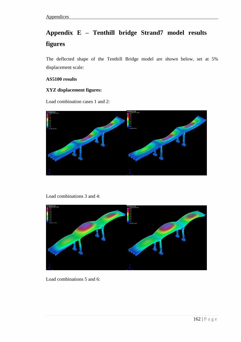
Appendices
162 | P a g e
Appendix E – Tenthill bridge Strand7 model results
figures
The deflected shape of the Tenthill Bridge model are shown below, set at 5%
displacement scale:
AS5100 results
XYZ displacement figures:
Load combination cases 1 and 2:
Load combinations 3 and 4:
Load combinations 5 and 6:
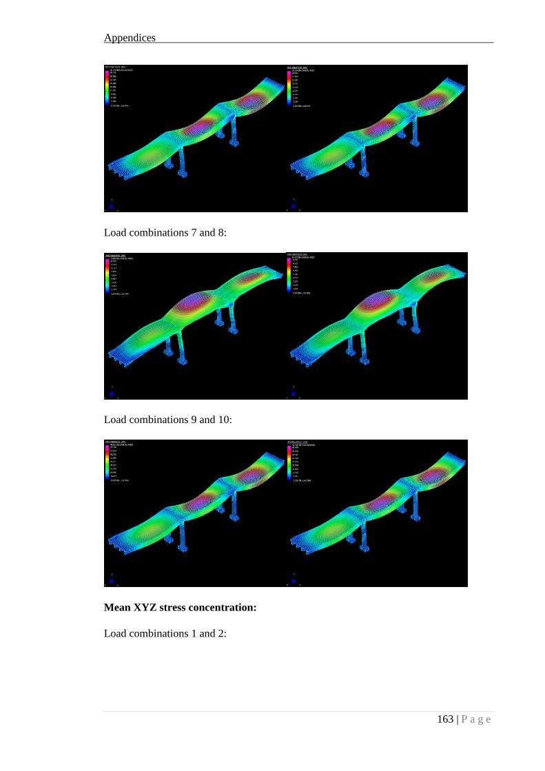
Appendices
163 | P a g e
Load combinations 7 and 8:
Load combinations 9 and 10:
Mean XYZ stress concentration:
Load combinations 1 and 2:

Appendices
164 | P a g e
Load combinations 3 and 4:
Load combinations 5 and 6:
Load combinations 7 and 8:

Appendices
165 | P a g e
Load combinations 9 and 10:
BA 59/94 results
XYZ displacement results:
Mean stress concentration results:

Appendices
166 | P a g e
AASHTO results
Displacement results:
Stress concentration results:

Appendices
167 | P a g e
Indian Code of Practice Results:
Displacement results:
Stress concentration results:

Appendices
168 | P a g e

Appendices
169 | P a g e
Appendix F – Resource Requirements
Resources that will be utilised in this project consists of project specific software
including:
Licenses and software locks
A computer capable of running the required software and reading the data
The project specific software utilised in this project consists of Strand7. The University
of Southern Queensland has access to the required software and the associated licenses
and software locks, therefore the simulations will be run on the computers located in Z-
block at USQ. Due to a limited amount of access time (8:00am to 5:00pm) to the computer
laboratories during the day, after-hours access was granted to the author (8:00am to
12:00am). The networked computer laboratories used for this project are:
Z308 – CATLab: CAD laboratory
Z310/Z311 – General-purpose PC workstations

Appendices
170 | P a g e
Appendix G – Risk Assessment
The risks associated with the activity are minimal from a physical point of view. A
possible physical risk could be staring at a computer screen for extended periods of time
which could result in eye strain, fatigue and/or stress. This could be avoided by taking
regular breaks, as well as having plenty of water and food available.
The risks of damage are somewhat more prevalent as the computer software, hardware
and data files could be damaged. The strategies for avoiding these situations are as
follows:
All of the data and files used in the project will be copied to an external hard drive
that is stored at the home of the author. Therefore if any data is lost or corrupt, the
data and files can be easily re-obtained.
Furthermore, as the simulations will be run on the Universities computers, there could be
unexpected hardware, network access, software and printing problems. If any problems
are to arise, they will be reported to the ICT Help Desk.


![Effect of Constitutive Model on Thermomechanical Fatigue ... · subjected automotive powertrain components to severe thermomechanical fatigue (TMF) loadings [1]. The design against](https://img.dokumen.tips/doc/110x75/5e932c9e8a6031207607f5b6/effect-of-constitutive-model-on-thermomechanical-fatigue-subjected-automotive.jpg)