Analysis of animal accelerometer data using hidden Markov models

Vianey Leos-Barajasa∗, Theoni Photopouloub, Roland Langrockc, Toby A. Pattersond, Yuuki

Watanabee, Megan Murgatroydb and Yannis P. Papastamatiouf,g

aIowa State University, USA; bUniversity of Cape Town, South Africa; cBielefeld University, Germany; dCSIRO,

Oceans and Atmosphere, Australia; eNational Institute of Polar Research, Japan; fUniversity of St Andrews, UK;

gFlorida International University, USA

Abstract

1. Use of accelerometers is now widespread within animal biotelemetry as they provide a means of

measuring an animal’s activity in a meaningful and quantitative way where direct observation is not

possible. In sequential acceleration data there is a natural dependence between observations of movement

or behaviour, a fact that has been largely ignored in most analyses.

2. Analyses of acceleration data where serial dependence has been explicitly modelled have largely relied

on hidden Markov models (HMMs). Depending on the aim of an analysis, either a supervised or an

unsupervised learning approach can be applied. Under a supervised context, an HMM is trained to classify

unlabelled acceleration data into a finite set of pre-specified categories, whereas we will demonstrate how

an unsupervised learning approach can be used to infer new aspects of animal behaviour.

3. We will provide the details necessary to implement and assess an HMM in both the supervised and

unsupervised context, and discuss the data requirements of each case. We outline two applications to

marine and aerial systems (sharks and eagles) taking the unsupervised approach, which is more readily

applicable to animal activity measured in the field. HMMs were used to infer the effects of temporal,

atmospheric and tidal inputs on animal behaviour.

4. Animal accelerometer data allow ecologists to identify important correlates and drivers of animal

activity (and hence behaviour). The HMM framework is well suited to deal with the main features

commonly observed in accelerometer data, and can easily be extended to suit a wide range of types of

animal activity data. The ability to combine direct observations of animals activity and combine it with

statistical models which account for the features of accelerometer data offer a new way to quantify animal

behaviour, energetic expenditure and deepen our insights into individual behaviour as a constituent of

populations and ecosystems.

Keywords: animal behaviour; activity recognition; latent states; serial correlation; time series

∗Corresponding author:e-mail: vianey@iastate.eduaddress: Snedecor Hall, Ames IA, Zip:50011phone number: 515-509-5388

1

arX

iv:1

602.

0646

6v1

[q-

bio.

QM

] 2

0 Fe

b 20

16

1 Introduction

Accelerometers are becoming more prevalent in the fields of animal and human biotelemetry (Bao & Intille,

2004; Ravi et al., 2005; Shepard et al., 2008; Altun et al., 2010). The potential of accelerometers lies in

the fact that they provide a means of measuring activity in a meaningful and quantitative way where direct

observation is not possible (Shepard et al., 2008; Nathan et al., 2012; Brown et al., 2013). While these

instruments are cheap and compact, recording acceleration at a high temporal resolution and in up to three

dimensions quickly results in terabytes of data that present various challenges regarding transmission, storage,

processing and statistical modelling.

Much of the focus in the analysis of acceleration data has been on identifying patterns in the observed

waveforms that correspond to a known behaviour or movement mode. This can be achieved by employing

statistical classification methods and entails observing the animal, manually assigning labels corresponding

to behaviours to segments of the data, and training a model using the labelled data in order to subsequently

classify remaining unlabelled data. There are many papers that have shown the effectiveness of various

machine learning algorithms for classification of human acceleration data (Bao & Intille, 2004; Ravi et al.,

2005; Altun et al., 2010; Mannini & Sabatini, 2010). Algorithms such as support vector machines (SVM),

classification trees, random forests, among others, have also recently been used for classification of animal

acceleration data (Nathan et al., 2012; Carroll et al., 2014; Graf et al., 2015). For example, Nathan et al.

(2012) compared the effectiveness of five machine learning algorithms to distinguish between eating, running,

standing, active flight, passive flight, general preening and lying down, for griffon vultures.

Most machine learning algorithms assume independence between individual observations. However, in

sequential acceleration data there is a natural dependence between observations of movement or behaviour

— once initiated, particular animal behaviours often last for periods longer than the sampling frequency.

This fact has been largely ignored in most applications of classification approaches. The studies where serial

dependence has been explicitly modelled have largely relied on hidden Markov models (HMMs) (Ward et al.,

2006; He et al., 2007; Mannini & Sabatini, 2010, 2011). Typically, and in common with the aforementioned

machine learning approaches, in the training stage, the states of the HMM were known a priori, requiring

corresponding data derived from direct observations.

There are two main difficulties with such a supervised learning approach. First, while there has been

much success in classification of human acceleration data, where training data can usually be obtained with

minimal effort, this may not be feasible for some animals. Humans can easily be observed in a laboratory

setting, given instructions, or monitored in more realistic settings, such as walking outdoors or in their home.

In certain cases, animals can also be monitored in a laboratory setting, but movement patterns recorded in

the lab from free-ranging animals may not appear exactly the same as in data collected while in more natural

settings. Conversely, many behaviours can only be observed in natural settings (Shepard et al., 2008; Nathan

et al., 2012; Brown et al., 2013).

Second, human acceleration data has commonly been used as a tool for health monitoring and other

situations where the focus is on (state) prediction, as opposed to learning how external factors drive the

behaviours. Classification of behaviours alone, while certainly of interest in many scenarios, may not lead

2

to biologically interesting inference. Once the classification has been done, the task of relating these states

to environmental (and other) covariates in order to identify drivers in behaviours remains. Moreover, as the

classifications are not without error it is difficult to make appropriate inferential statements, propagating

the state uncertainty through to the modelled effect of the covariates. These difficulties will arise in any

classification method.

In the supervised context, i.e. when classification is the main purpose of an analysis, we train the HMM

to recognize specific behaviours. Alternatively, HMMs can also be used in an unsupervised context, i.e.

when there are no labelled data. In an unsupervised context the states are not pre-defined to represent a

specific behaviour, and instead will be allocated such that the model captures as much as possible of the

marginal distribution of the observations as well as their correlation structure. If biologically meaningful

response variables from the acceleration data are considered, then the HMM states will usually represent

interpretable activity levels or even proxies of behavioural modes. Being data-driven the states can be as, if

not more, informative in the unsupervised setting than the alternative. We can then incorporate exogenous

or, where available, endogenous variable(s) of interest, to make inferential statements. HMMs and related

state-switching models, in particular state-space models, have successfully been implemented to identify

drivers of movement based on tracking data (Patterson et al., 2009), and can similarly be applied in the

context of accelerometer data.

In this paper we review HMM-based approaches to the analysis of animal accelerometer data. In Section

2 we will provide an overview of accelerometer data and connect the data processing step to the HMM-based

approaches described in Section 3. In Section 4 we demonstrate the use of HMMs with real data examples

from marine and aerial systems.

2 Accelerometer data

Accelerometer devices measure in up to three axes, which can be described relative to the body of the animal;

longitudinal, lateral and dorso-ventral. Acceleration recorded along one or two axes can be used to measure

movement in parts of the body, e.g. the mandible (Suzuki et al., 2009; Naito et al., 2010; Iwata et al., 2015),

or aspects of whole body acceleration, e.g. longitudinal surge in Sakamoto et al. (2009). Currently, acceler-

ation is most commonly recorded in three axes, and to a lesser degree, in two axes (Brown et al., 2013), to

measure locomotion. Especially for flying or swimming animals, measuring in all three axes is essential for

capturing all movements performed by the animal, since movement is inherently three-dimensional. However,

the resolution of acceleration is key to enabling identification of behaviours from the raw data.

Data Processing for Classification

Although the observed (raw) acceleration data can be used to identify specific movements in animals,

HMMs and other machine learning algorithms typically require more than that to accurately classify the

unlabelled data. These methods will require appropriate features, i.e. summary statistics. In most cases, and

3

as will be described here, a window size is selected and multiple features are calculated from the observations

corresponding to each window. The window size can correspond to a number of observations or can also be

a sliding window such that there is some percentage of overlap between consecutive windows.

The derived features should be driven by the classes of movements that have been defined and chosen

in such a way to accentuate the differences in observed acceleration measurements. For example, for each

window we can compute the mean, variance, dynamic body acceleration, pitch, correlation among axes (and

the list goes on). No optimal set of features exists although there are many commonalities between those used

in applications of classification of acceleration data (Bao & Intille, 2004; Martiskainen et al., 2009; Nathan

et al., 2012; Brown et al., 2013). For instance, Nathan et al. (2012) used thirty-eight features in order to

distinguish between eating, running, standing, active flight, passive flight, general preening and lying down,

for griffon vultures, while Graf et al. (2015) used eight features to distinguish between standing, walking,

swimming, feeding, diving and grooming of Eurasian beavers. In each case, means and variances of each of

the three axes are used, as well as overall dynamic body acceleration (ODBA), the sum of dynamic body

acceleration from the three axis, among others.

Connecting Measures to Behaviours

When the aim is to classify the acceleration data, data processing is driven by identifying a set of fea-

tures that can be used to distinguish between specific movements, even if those features are not themselves

interpretable as a specific behaviour when considered on their own. However, there are metrics derived from

the accelerometer data that, on their own, can be used as proxies for behaviour and as input to an HMM.

There can be a number of diverse signals corresponding to different movement behaviours. Repeating

patterns in at least one axis tend to arise from regular movement such as stroking (Sakamoto et al., 2009),

flapping, running or walking (Shepard et al., 2008), whereas sudden changes, corresponding to bursts of

acceleration, are often associated with prey pursuits or capture (Suzuki et al., 2009; Simon et al., 2012;

Ydesen et al., 2014; Heerah et al., 2014), as well as predator avoidance, or conflict.

In addition to behaviour, several measures can be used to summarise effort or exertion and relate accel-

eration to energy expenditure or activity levels. These include overall dynamic body acceleration (ODBA)

(Wilson et al., 2006; Gleiss et al., 2011; Elliott et al., 2013; Gleiss et al., 2013) and vectorial dynamic body

acceleration (VeDBA) (Qasem et al., 2012), while minimum specific acceleration (MSA) (Simon et al., 2012)

can be used to disentangle the gravitational component of acceleration (static acceleration) from the move-

ment signal, or specific acceleration (also dynamic acceleration). One of the simplest and most unambiguous

interpretations of static acceleration data is body posture, which in many cases can be directly interpreted

as a specific behaviour (Wilson et al., 2008; Shepard et al., 2008).

Speed is an important aspect of animal movement since it is often related to energy expenditure or energy

acquisition. Speed can be calculated using acceleration and depth data from marine animals during diving,

when the pitch angle is steep (Watanabe et al., 2003; Shepard et al., 2008). Stroke frequency in aquatic

animals such as sharks (Watanabe et al., 2012), whales, seals (Sato et al., 2003), and diving seabirds (Sato

4

et al., 2008) can be used both as a measure of activity and, in some cases, a measure of foraging success

(Sato et al., 2008). It has also been shown that acceleration can be used to distinguish between different

flight behaviours in soaring birds (Williams et al., 2015).

3 Analysis of accelerometer data

We will first provide a brief overview of the HMM framework (Section 3.1). Subsequently, in Section 3.2, we

will review how HMMs can be used for classification of animal accelerometer data. In Section 3.3, we focus

on the implementation of HMMs in an unsupervised setting, such that the meaning of the states is driven

entirely by the data and the focus lies on general inference rather than classification only.

3.1 Hidden Markov models

An HMM is a stochastic time series model involving two layers: an observable state-dependent process,

denoted by {Yt}Tt=1 (in the univariate case), and an unobservable state process, denoted by {Ct}Tt=1. The

state-dependent process models the observations, while the state process is a latent factor influencing the

distribution of the observations. In our case, the observations are the accelerometer metrics considered, and

the latent states are closely related to the animal’s behavioural state. More specifically, the state process {Ct}takes on a finite number of possible values, 1, . . . ,M , and its value at time t, ct, selects which of M possible

component distributions generates observation yt. The Markov property is assumed for {Ct}, such that

evolution of the process over time is completely characterized by the one-step state transition probabilities.

These models are natural and intuitive candidates for modelling animal accelerometer data, for two rea-

sons: 1) they directly account for the fact that any corresponding observation will be driven by the underlying

behavioural state, or general activity level, of the animal, and 2) they accommodate serial correlation in the

time series by allowing states to be persistent. HMMs seek to capture the strong autocorrelation in accelerom-

eter data in a mechanistic way, rather than either neglecting this feature completely or only including it in a

nuisance error term. HMMs can therefore be used for inference on complex temporal patterns, including the

behavioural state-switching dynamics and how these are driven by environmental variables.

To complete the basic HMM formulation, we first summarize the probabilities of transitions between

the different states in the M ×M transition probability matrix (t.p.m.) Γ = (γij), where γij = Pr(Ct =

j|Ct−1 = i)

(for any t), i, j = 1, . . . ,M . Note that here we are assuming that the state transition probabilities

are constant over time; this assumption will be relaxed in Section 3.3. The initial state probabilities are

summarized in the row vector δ, where δi = Pr(C1 = i), i = 1, . . . ,M .

Second, we need to specify state-dependent distributions (sometimes called emission distributions), p(yt|Ct =

m), or more succinctly pm(yt), for m = 1, ...,M . These distributions can be discrete or continuous, and pos-

sibly also multivariate (in which case we write yt = (y1t, . . . , yRt)). Usually, the same parametric distribution

is assigned to all M states, such that each state differs in terms of its associated values of the parameters.

Selection is driven by the data itself, e.g. count data or continuous observations.

5

3.2 Classification based on supervised learning

HMMs provide a solid framework for the classification of data with strong serial dependence, such as se-

quential acceleration data, which are often processed to represent movements over a few seconds, or less,

at a time (Ward et al., 2006; He et al., 2007; Mannini & Sabatini, 2010). In this section, we will cover the

implementation and testing of an HMM when there are labelled data available and the aim is to categorize

unlabelled data into a finite set of pre-defined classes, with a low error rate.

In supervised learning, the collection of labelled time series is split into three categories: training data,

validation data, and testing data. An approximate split of 50%, 25%, 25% can be used (Hastie et al., 2001),

although this will require splitting the observations in such a way that takes into account the temporal

dependence and possible multiple time series from the same animal. The training data will be used to fit

the HMM, the validation data is used for model selection, and the testing data will be used to estimate the

prediction error for the final model selected. We can test a variety of HMM formulations and select the best

performing among them.

However, in many cases there will only be sufficient data to split into training and testing, in which

case multiple approaches can be taken for model selection/assessment, as described in Hastie et al. (2001).

Cross-validation is one of the most common approaches to estimate prediction error. If the K time series

are independent of each other, we can use leave-one-out cross-validation treating each time series as an

observation. We fit the HMM to K − 1 time series, the training data, and decode the state sequence of

the time series left out, the testing data, using the parameter estimates of the fitted model, in order to

compare our predictions to the known state sequence. This process is repeated K times. (Leave-one-out

cross-validation is one approach that can be taken, but certainly not the only one, and is only used here for

illustrative purposes.)

In the training stage, the state sequence is known which greatly simplifies fitting the HMM. If the sequence

of states, c1, . . . , cT , is known, then we obtain the (complete-data) likelihood of the HMM for one time series

as

LC = p(c1 . . . , cT ,y1 , . . . ,yT ) = δc1 pc1 (y1 )

T∏t=2

γct−1 ,ct pct (yt). (1)

For K independent time series, the likelihood is the product of the individual complete-data likelihoods. For

an HMM in the context of classification, each state-dependent distribution is often selected to be a multivariate

normal distribution (MVN), or a mixture of MVNs if the data are highly non-normal. The MVN is commonly

used as it can model the dependence between random variables, in our case the R features that will be used

for classification. (Alternatively, one can assume conditional independence between all features, given the

states, such that the joint density, p(yt|Ct = m), can be written as p(yt|Ct = m) =∏R

r=1p(yrt|Ct = m).)

We will use the MVN to illustrate the procedures for training an HMM for classification of unlabelled data.

The density of the state-dependent MVN is

p(yt|Ct = m) =1

(2π)R/2|Σm|1/2exp

(−1

2(yt − µm)>Σ−1m (yt − µm)

),

6

where µm and Σm are the vector of state-dependent means (of the R variables) and the state-dependent

covariance matrix, respectively. These need to be estimated for each state m, alongside the state transition

probabilities and the initial state distribution. Thus, we maximize (1) (or, in case of multiple time series, a

product of likelihoods of type (1)) with respect to δ, Γ, µm and Σm, m = 1, . . . ,M , to obtain the maximum

likelihood estimates (MLEs). Since the states are known the maximization task conveniently splits into

several independent parts, each of which is fairly straightforward. First, the m-th entry of δ is simply the

proportion of the time series that start in state m. Second, the entries of the t.p.m. are estimated by

γij =# transitions from state i to state j

total # transitions from state i,

for i, j = 1, ...,M . (Note this is the MLE conditional on the initial state, c1.) Finally, µm and Σm are

estimated using only the observations allocated to state m.

Given a fitted HMM, two state-assignment approaches can be used in the testing stage: local or global de-

coding. Local decoding assigns a state at each time t by maximising the conditional probability Pr(Ct|Y1, . . . ,YT ),

under the fitted model. Global decoding maximises Pr (C1, . . . , CT |Y1, . . . ,YT ) to assign the most likely se-

quence of states for the entire time series. A dynamic programming algorithm, the Viterbi algorithm, can

be used to find the optimal state sequence at low computational effort. While the outcome is usually very

similar, it does sometimes happen that the decoded states differ. Essentially Viterbi considers the state

sequence as a whole, while local decoding considers each time point in isolation. Full details are provided in

Zucchini and MacDonald (2009). The state predictions are compared to the known states, and the proportion

of correctly decoded states serves as an estimate of the prediction accuracy.

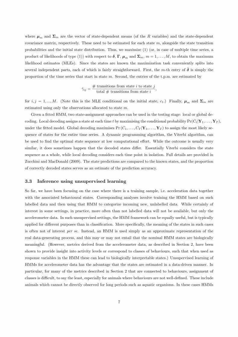
3.3 Inference using unsupervised learning

So far, we have been focusing on the case where there is a training sample, i.e. acceleration data together

with the associated behavioural states. Corresponding analyses involve training the HMM based on such

labelled data and then using that HMM to categorize incoming new, unlabelled data. While certainly of

interest in some settings, in practice, more often than not labelled data will not be available, but only the

accelerometer data. In such unsupervised settings, the HMM framework can be equally useful, but is typically

applied for different purposes than in classification. More specifically, the meaning of the states in such cases

is often not of interest per se. Instead, an HMM is used simply as an approximate representation of the

real data-generating process, and this may or may not entail that the nominal HMM states are biologically

meaningful. (However, metrics derived from the accelerometer data, as described in Section 2, have been

shown to provide insight into activity levels or correspond to classes of behaviours, such that when used as

response variables in the HMM these can lead to biologically interpretable states.) Unsupervised learning of

HMMs for accelerometer data has the advantage that the states are estimated in a data-driven manner. In

particular, for many of the metrics described in Section 2 that are connected to behaviours, assignment of

classes is difficult, to say the least, especially for animals where behaviours are not well-defined. These include

animals which cannot be directly observed for long periods such as aquatic organisms. In these cases HMMs

7

have been shown to be useful. For example, Phillips et al. (2015) applied HMMs using MVN responses of

behavioural indices but in an unsupervised context to understand the behaviour of free swimming tuna from

vertical movement data collected by data-storage tags. Below we demonstrate the application of unsupervised

learning for another difficult to observe species, namely blacktip reef sharks.

There are three different possible purposes of having an approximate representation of the real process: (i)

a description of the stochastic structure of the system; (ii) extraction of information; (iii) prediction (Konishi

& Kitagawa, 2008). In the ecological literature on animal movement modelling, HMMs are used primarily to

address (i) and (ii), the former in the sense that concise descriptions of movement patterns are sought, the

latter in the sense that inference on the interaction of animals with their environment is drawn. In general,

the ability to make inferential statements provides an avenue to answer questions about the behavioural

processes, movement patterns and transitions between behaviours under different conditions or in relation to

other covariates.

Addressing a research question related to aim (ii) usually involves the incorporation of covariates into

the statistical model. In the HMM setting, this is commonly done at the level of the hidden states. For the

general case of time-varying covariates, we define the corresponding time-dependent transition probability

matrix Γ(t) = (γ(t)ij ), where γ

(t)ij = Pr(Ct+1 = j|Ct = i). The transition probabilities at time t, γ

(t)ij , can then

be related to a vector of environmental (or other) covariates,(ω(t)1 , . . . , ω

(t)p

), via the multinomial logit link:

γ(t)ij =

exp(ηij)∑Nk=1 exp(ηik)

, where ηij =

β(ij)0 +

∑pl=1 β

(ij)l ω

(t)l if i 6= j;

0 otherwise.

Essentially there is one multinomial logit link specification for each row of the matrix Γ(t), and the entries

on the diagonal of the matrix serve as reference categories.

While with labelled data the likelihood of interest is the complete-data likelihood given in (1) (i.e. the

joint density of observations and states), for unlabelled data the likelihood of interest is the density of the

observations only, L = p(y1 , . . . ,yT ), the evaluation of which requires the consideration of all possible state

sequences that might have given rise to these data. Given the simplicity of the complete-data likelihood, it

comes as no surprise that the expectation-maximization (EM) algorithm is seen as a natural approach to deal

with this complexity. The EM algorithm is an iterative scheme for finding the MLEs, and involves alternate

updates of the conditional expectation of the states (given the data and the current estimates) and updates

of the model parameters based on the complete-data log-likelihood where the unknown states are replaced by

their conditional expectations. Despite the intuitive appeal of EM, as pointed out for example by MacDonald

(2014), there is a more direct route to MLEs, namely direct numerical maximization of the likelihood. Since

it is our view that users are better off focusing on the simpler direct maximization approach, it is only this

approach that we present here in detail.

In order to efficiently calculate (and numerically maximize) the likelihood, rather than separately con-

sidering all MT possible hidden state sequences that might have given rise to the observations, which in

general is infeasible, the HMM dependence structure can be exploited to perform the likelihood calculation

8

recursively, traversing along the time series and updating the likelihood and state probabilities at every step.

To do so, we define the forward probability of state j at time t as αt(j) = p(y1, ...,yt, ct = j). Due to the

dependence structure, we have

αt(j) = p(yt | y1, ...,yt−1, ct = j)p(y1, ...,yt−1, ct = j)

= p(yt | ct = j)

M∑i=1

p(y1, ...,yt−1, ct = j, ct−1 = i)

= p(yt | ct = j)

M∑i=1

p(ct = j | y1, ...,yt−1, ct−1 = i)p(y1, ...,yt−1, ct−1 = i)

=

M∑i=1

αt−1(i)γ(t−1)ij pj(yt).

In matrix notation, defining the vector of forward probabilities at time t as αt =(αt(1), . . . , αt(M)

), this

becomes αt = αt−1Γ(t−1)Q(yt), where Q(yt) = diag

(p1(yt), . . . , pM (yt)

). Together with the initial calcula-

tion α1 = δQ(y1), this is the so-called forward algorithm. The forward algorithm can be applied in order to

first calculate α1, then α2, etc., until one arrives at αT . The likelihood then simply is L =∑M

m=1 αT (m).

The computational cost of evaluating the likelihood is linear in the number of observations, T , such that

a numerical maximization of the likelihood becomes feasible in most cases. The structure of the likelihood

evaluation is independent of the type of state-dependent distributions applied. In other words, changing the

class of distributions used for the observations leads to minimal changes in the code, since only the matrices

Q(yt) need to be modified. The same holds for the specification of the transition probabilities (with or

without dependence on covariates).

Model selection techniques, in particular information criteria, can be used to choose an adequate family

of state-dependent distributions, to select an appropriate number of states, or to determine whether or not a

covariate should be included in the model. However, users should not blindly follow such information criteria,

especially with regard to the selection of the number of states. For animal behaviour data, in our experience

such formal model selection approaches tend to favour overly complex models, often to an extent such that

selected models become near-impossible to interpret and very difficult to work with in practice (Langrock

et al., 2015). One explanation for this is that, while clearly natural and appealing, HMM-type models are

usually still very simplistic relative to the actual behavioural decisions and hence the data-generating process.

A model selection scheme might then point to a model where minor, possibly irrelevant features of the data

that are not well described by say a simple two-state or three-state model are captured by additional states,

often such that these are rarely ever visited by the animal considered. While corresponding models might of

course better explain the data at hand, it often turns out that meaningful inference is severely hindered by

models with complex state architectures. In such cases a healthy dose of pragmatism is required. Applying

nonparametric state-dependent distributions, as suggested by Langrock et al. (2015), is one strategy for

avoiding overly complex state processes.

The HMM framework encompasses various other useful tools for drawing inference, including, inter alia,

the option to incorporate random effects to account for individual heterogeneity (McKellar et al., 2015)

9

and (pseudo-)residuals for comprehensive model checks (Zucchini and MacDonald, 2009). Furthermore, the

dependence structure can be modified in various ways, e.g. allowing for more complex memory in the state

process (Langrock et al., 2012) without losing the ability to efficiently calculate the likelihood.

4 Real data examples

4.1 Modelling activity in a soaring raptor

Large soaring birds like raptors rely heavily on meteorological conditions and underlying topography for

generation of the updrafts necessary for low-energy flight. However, the relationships between different

weather conditions and bird activity patterns are not well understood. In addition, the same conditions that

are favourable for soaring flight are often also favourable for the generation of renewable energy from wind.

Rotating wind turbines pose a threat to many bird species, so understanding the conditions under which birds

spend most time active can be important at prospective installation sites (Katzner et al., 2013; Rushworth

& Kruger, 2014). Acceleration data, in combination with other types of movement data, hold promise in

distinguishing between different kinds of flight behaviour and how active each flight behaviour is, in soaring

birds (Williams et al., 2015).

0

1

2

3

17 Apr 18 Apr 19 Apr 20 Apr 21 Apr 22 Apr 23 Apr 24 AprDate

MS

A

MSA values for 16 to 24 April

Figure 1: Minimum specific acceleration values derived from three-axis acceleration data from one eaglecollected over 9 days, 16-24 July 2013.

Acceleration data were collected for an adult Verreaux’s eagle (Aquila verreauxii) in the Western Cape,

South Africa, in 2013, instrumented with a remotely downloadable multi-sensor data-logger (UvABiTS,

University of Amsterdam, The Netherlands). Data were collected over a one-second sampling period at a

resolution of 20Hz and at intervals of 112sec, for 9 days (Figure 1). Each day contained a variable number of

acceleration samples. Because of the discontinuous nature of the data, we used minimum specific acceleration

(MSA) to extract an index of activity from the three-axis acceleration data. We were not interested in the

pattern of MSA within the one-second sample so we took the maximum value from each one-second sample.

This resulted in 1429 observations, with a mean number of 158.78 observations per day (SE 26.67), which

equates to an observation period of approximately 5 hrs per day, on average. Data were not collected at

night which created gaps between daytime bouts of observations.

No concurrent direct observations were available, so it was not possible to link distinct behaviours with

different values of MSA. Instead, we used MSA as a proxy for activity and fitted a 2-state HMM to investi-

10

gate the effect of wind speed and temperature on bird activity. Without considering any ancillary data, it

seemed sensible to assume two states, one including low-level activity, and the other more active movement.

Preliminary data analysis revealed that MSA showed two peaks close to zero, suggesting that two types of

movement comprise the less active state. We chose to formulate a model that would lump these two types of

activity levels together in one state, since the interest lies in identifying higher-level energetic activity, such as

flapping and hunting, instead of discriminating between, for example, being completely stationary (roosting)

and preening or being otherwise alert. Therefore, we implemented a mixture of two Gamma distributions as

the state-dependent probability distribution for the less active state to account for these two processes, and

a single Gamma distribution in the more active state.

Since there were long gaps between the data collected on different days (due to the absence of any night-

time observations), we treated the observations from each day as a separate, independent time series. We

fitted the model jointly to all maximum MSA values, collected on the nine days of observation, and estimated

global parameters across all segments.

Lift availability is known to be driven largely by wind speed and temperature, as well as their interaction

with the underlying topography, though other factors also contribute. Lift adequate for soaring flight is

generated by two mechanisms; (1) by upward thermal convection of air warmed by solar radiation (Akos

et al., 2010) (thermal soaring), and (2) by the movement of air over slopes and ridges in the landscape

(orographic or ridge soaring). Activity levels in raptors are expected to vary throughout the day but we

chose not to include time of day as a covariate for the t.p.m. because what drives this pattern is most likely

the environmental variables, such as the building heat of the day and associated convection, rather than the

time of day itself (though prey availability is also an important factor not considered here). April is autumn

in Southern Africa which can be very warm in the day, but is still cool overnight and is characterised by fairly

light winds relative to summer. The range of temperatures and wind speeds experienced by the bird during

the study period ranged between 12.3 and 31.5 ◦C, and 0 and 7.4 m/sec. In this example we only examine

the effects of meteorological variables on the t.p.m. To capture the effect of wind and solar radiation on the

probability of transitioning between states, we included wind speed, temperature and their interaction in the

model as covariates affecting the entries of the t.p.m. The model including wind speed alone was favoured by

the Bayesian Information Criterion (BIC) and the Akaike Information Criterion (AIC) (Table 1). The fitted

state-dependent densities are shown in Figure 2.

Model Log-likelihood AIC ∆ AIC BIC ∆ BIC

No covars 2344.8 -4665.6 23.7 -4602.4 23.1Temperature 2347.4 -4670.9 17.8 -4607.7 17.8Wind speed 2356.4 -4688.7 0 -4625.5 0Wind speed, Temperature 2356.4 -4688.1 0.6 -4614.4 11.1Wind speed, Temperature, 2358.5 -4684.9 3.8 -4600.7 24.8

Wind speed * Temperature

Table 1: Model fitting results for a Verreaux’s eagle. Based on the AIC and BIC, the model selected includesonly wind speed.

The estimated state transition probabilities suggest that, as wind speed increases, (i) the eagle has a

11

0

20

40

60

0.0 0.5 1.0 1.5 2.0Minimum specific acceleration (MSA)

Den

sity

State−Dependent MSA Densities

4e−048e−04

2.00 2.25 2.50 2.75 3.00Minimum specific acceleration (MSA)

Den

sity Tail behaviour of Densities

0

10

20

30

40

0.0 0.5 1.0 1.5 2.0Minimum specific acceleration (MSA)

Den

sity

DensitiesMarginalState 1State 2

Marginal MSA Density

Figure 2: Histogram of minimum specific acceleration, truncated at MSA=2, with marginal density andstate-dependent densities weighted according to the proportion of observations assigned to each state. (left).Unweighted state-dependent densities (top right) and close-up of the tail behaviour of the densities (bottomright). A square root coordinate transformation for the x-axis was used in all plots and for the y-axis onlyfor the tail behaviour plot.

0.00

0.25

0.50

0.75

1.00

0 2 4 6Wind speed (m/sec)

Pro

babi

lity

State 1 −> State 1State 2 −> State 2

State Dwell Probabilities

0.00

0.25

0.50

0.75

1.00

0 2 4 6Wind speed (m/sec)

Pro

babi

lity

State 1State 2

Stationary Distribution

Figure 3: Estimated state-dwell probabilities as a function of wind speed (left), and estimated equilibriumstate probabilities as a function of wind speed (right).

very slightly increased chance of switching to the high-activity state when in the low-activity state, and

(ii) generally spends much longer periods of time, on average, in the active state. As a consequence, the

equilibrium (stationary) distribution for fixed wind speeds (Patterson et al., 2009) indicates that the bird

spends more time in the active state overall as wind speed increases (Figure 3). If the active state is

representing orographic soaring, this would be consistent with the results of studies on migrating golden

eagles Aquila chrysaetos which also did more orographic soaring as a response to higher wind speed Lanzone

et al. (2012). The fact that temperature was not found to have a strong effect is somewhat surprising since

one would expect high temperatures to be conducive to the formation of thermals and thermal soaring, and

12

the appearance of a signal in the MSA data pointing towards activity. However, it may be that thermal

soaring is a low-effort behaviour, compared to orographic soaring, and does not result in a peak in activity,

as measured by the MSA. Alternatively, perhaps there were other factors in play during the study period,

which made thermal soaring a less cost-effective mode of transport and the bird simply did not engage in

that behaviour consistently.

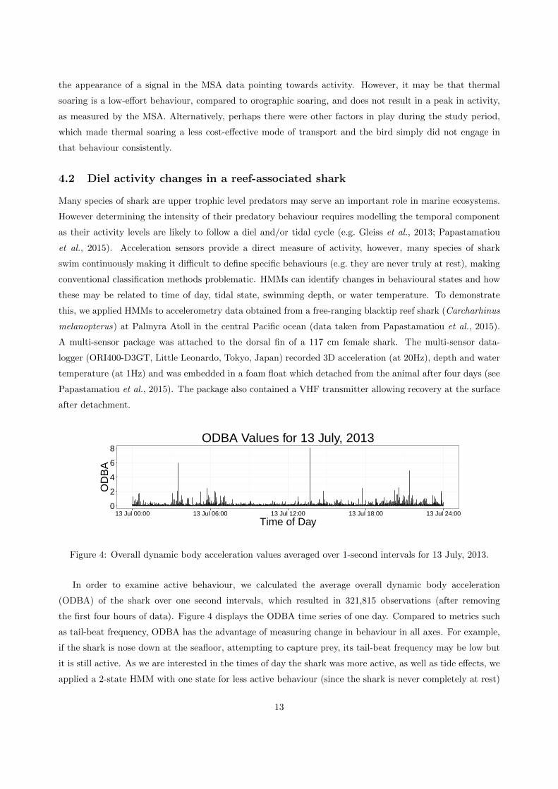
4.2 Diel activity changes in a reef-associated shark

Many species of shark are upper trophic level predators may serve an important role in marine ecosystems.

However determining the intensity of their predatory behaviour requires modelling the temporal component

as their activity levels are likely to follow a diel and/or tidal cycle (e.g. Gleiss et al., 2013; Papastamatiou

et al., 2015). Acceleration sensors provide a direct measure of activity, however, many species of shark

swim continuously making it difficult to define specific behaviours (e.g. they are never truly at rest), making

conventional classification methods problematic. HMMs can identify changes in behavioural states and how

these may be related to time of day, tidal state, swimming depth, or water temperature. To demonstrate

this, we applied HMMs to accelerometry data obtained from a free-ranging blacktip reef shark (Carcharhinus

melanopterus) at Palmyra Atoll in the central Pacific ocean (data taken from Papastamatiou et al., 2015).

A multi-sensor package was attached to the dorsal fin of a 117 cm female shark. The multi-sensor data-

logger (ORI400-D3GT, Little Leonardo, Tokyo, Japan) recorded 3D acceleration (at 20Hz), depth and water

temperature (at 1Hz) and was embedded in a foam float which detached from the animal after four days (see

Papastamatiou et al., 2015). The package also contained a VHF transmitter allowing recovery at the surface

after detachment.

0

2

4

6

8

13 Jul 00:00 13 Jul 06:00 13 Jul 12:00 13 Jul 18:00 13 Jul 24:00

Time of Day

OD

BA

ODBA Values for 13 July, 2013

Figure 4: Overall dynamic body acceleration values averaged over 1-second intervals for 13 July, 2013.

In order to examine active behaviour, we calculated the average overall dynamic body acceleration

(ODBA) of the shark over one second intervals, which resulted in 321,815 observations (after removing

the first four hours of data). Figure 4 displays the ODBA time series of one day. Compared to metrics such

as tail-beat frequency, ODBA has the advantage of measuring change in behaviour in all axes. For example,

if the shark is nose down at the seafloor, attempting to capture prey, its tail-beat frequency may be low but

it is still active. As we are interested in the times of day the shark was more active, as well as tide effects, we

applied a 2-state HMM with one state for less active behaviour (since the shark is never completely at rest)

13

and another for more active behaviour.

0e+00

5e−04

1e−03

2 4 6 8 10Overall Dynamic Body Acceleration

Den

sity

Tail Behaviour of Densities

0

5

10

15

0.0 0.5 1.0 1.5 2.0Overall Dynamic Body Acceleration

Den

sity

State−Dependent ODBA Densities

0

5

10

0.0 0.5 1.0 1.5 2.0Overall Dynamic Body Acceleration (ODBA)

Den

sity

DensityState 1State 2Marginal

Marginal ODBA Density

Figure 5: Histogram of overall dynamic body acceleration, truncated at ODBA=2, with marginal density andstate-dependent densities weighted according to the proportion of observations assigned to each state. (left).Unweighted state-dependent densities (top right) and close-up of the tail behaviour of the densities (bottomright). A square root coordinate transformation for the x-axis was used in all plots and for the y-axis onlyfor the tail behaviour plot.

Although there are clear spikes in ODBA that point to higher energetic activities, various combinations of

parametric distributions for state 1 and 2 led to vastly different state-dependent densities. Further, the ODBA

values had many extreme values that needed to be accommodated, which further increased the difficulties of

selecting appropriate state-dependent distributions. As ODBA is not a metric that can easily be divided into

active/inactive behaviours in sharks, we estimated the state-dependent densities nonparametrically, in both

states, in order to minimize the bias introduced by assigning inadequate parametric distributions (Langrock

et al., 2015). Figure 5 displays the fitted distributions.

To examine potential diel and tide effects on activity levels, we let the entries of the t.p.m. be functions

of up to two covariates: time of day and tide level (ebb, flood, low, and high). Tide data was obtained from

the NOAA tides and currents website for Palmyra Atoll and was processed by denoting high or low tide as

±1 hour from reported high or low tide times. Time of day is represented by two trigonometric functions

with period 24 hours, cos(2πt/86400) and sin(2πt/86400) (86,400 is the number of seconds in a day). We use

three indicator variables, x1t, x2t and x3t, for tide levels high, flood, and ebb, respectively, so that the entries

of the t.p.m. have the following form

logit(γij(t)) = β0i + β1isin(2πt/86400) + β2icos(2πt/86400) + β3ix1t + β4ix2t + β5ix3t

for i = 1, 2, j 6= i, t = 1, . . . , 86400. The intercept term β0,i corresponds to low tide.

Based on the selected model (cf. Table 2), the shark’s activity levels were, on average, lowest from

approximately 9:00 – 13:00 and highest from 21:00 – 1:00. In Figure 6, we see that the shark was more active

14

Model Log-likelihood AIC ∆ AIC BIC ∆ BIC

No covariates 639299.2 -1278370 779 -1277178 692Time 639558.1 -1278872 277.2 -1277645 225Time, High 639657.6 -1279063 86.2 -1277819 51Time, High, Flood 639695.2 -1279130 19 -1277869 1Time, High, Flood, Ebb 639708.7 -1279149 0 -1277870 0

Table 2: Model fitting results for a blacktip shark. Based on the AIC and BIC, the model selected includestime of day and includes differences in activity levels based on all categories of tide levels.

0.2

0.3

0.4

0.5

00:00 06:00 12:00 18:00 24:00Time of Day

P(S

tate

2)

Result

Estimate

Forecast

TideLevels

Ebb

Flood

High

Low

Stationary Distribution for State 2

Figure 6: Implied stationary distribution for state 2, the more active state, by time of day and tide level.For tide levels, we distinguish between model estimates, such that the corresponding tide level was observedat that time of day, and forecasts.

during high tide in general when compared to flood, low or ebb tide. While the equilibrium (or stationary)

distribution associated with low and ebb tide overlap, the state-dwell probabilities are higher during ebb tide

than in low tide.

Using the Viterbi algorithm, we decoded the optimal state sequence of the ODBA time series. To further

understand the effect of vertical habitat on behaviour, we related the decoded state sequence results to a grid

of depth and temperature values, shown in Figure 7. The shark spent most of its time over the nearly five

day period in depths of about 3-6 metres and between 28-29 degrees Celsius, with some higher counts also in

shallower waters, which is reflected in the state 2 counts. However, the percentages of state 2 observations

reveals that the shark was generally more active when near the surface in waters of 28-29 degrees C. There

was generally less active behaviour exhibited when the individual was in very shallow warm water (> 29

degrees C).

15

0

2

4

6

8

10

28 29 30 31 32 33Temperature (in Celsius)

Dep

th (

m)

0

500

1000

1500

Count

No. of Observations in State 2

0

2

4

6

8

10

28 29 30 31 32 33Temperature (in Celsius)

Dep

th (

m)

0.00

0.25

0.50

0.75

1.00Percentage

% Observations in State 2

Figure 7: The number of observations in each grid cell that correspond to state 2. Zero counts appear inwhite. (left) Percentage of observations in each cell that correspond to state 2. (right)

5 Discussion

We considered two approaches for analysing animal accelerometer data with HMMs: a supervised learning

approach, such that classification is of primary interest, and an unsupervised learning approach. The aim of a

study and the type of data available will determine which of the two is to be preferred. When the objective is

to do classification and there is a set of pre-defined behaviours of interest, then the model’s ability to correctly

predict and categorize behaviours is of main interest. In this instance, a supervised learning approach may be

applied. One of the benefits of such an approach is that the behavioural classes are exactly defined, making

interpretation relatively straightforward. Alternatively, if the objective is to infer (or, colloquially speaking,

to ‘learn’) new aspects of animal behaviour, then the unsupervised approach provides an excellent framework.

The latter comes with the implicit caveat that the states will not necessarily map directly to specific animal

behaviours. Any post-hoc behavioural interpretation of the estimated states is directly connected to the

metric(s) used, and must draw from background biological knowledge of the species of interest. In many

16

cases, behaviours such as foraging may not be exclusive to one state or another. Nonetheless, if the model

is able to identify bouts of behaviour which consistently re-appear, then it is often likely that these signify

something important in the animal’s behavioural repertoire and are worthy of further investigation.

Even when classification is the goal of an analysis, there are certainly practical scenarios which preclude

the use of an HMM, e.g. if the training data do not reflect the transitions between behaviours or if there is

insufficient data. Multiple studies have shown that other machine learning algorithms, e.g. support vector

machines (SVM) or random forests, can work well for classification of animal acceleration data (Martiskainen

et al., 2009; Nathan et al., 2012; Carroll et al., 2014; Graf et al., 2015). However, disregarding the serial

dependence in the acceleration data usually is an unrealistic assumption, which often goes unmentioned or

is treated as an afterthought. Adopting the assumption of independence is particularly risky if inferential

statistics are applied to the output of say a machine learning algorithm. In these cases, secondarily applied

statistical tests will implicitly assume that the machine learning categorizations contain more information

content than is warranted, potentially leading to spurious results. This is not just a statistical nuance and

can be a crucial point. Such tests are often applied as decision making tools to sort out “what matters”

and setting the direction for much further research effort. Also, in assuming independence, one allows for

classifications that may not be biologically realistic or must filter the classifications to properly identify a

specific behaviour. For instance, Carroll et al. (2014) used a SVM where one of the primary interests was

to identify prey handling/capture for penguins at sea. To confirm a prey capture event, they ruled that if

the SVM classified three consecutive observations as prey-handling this counted as a true prey capture. In

contrast, an HMM would have bypassed the need to filter through the classification results by accounting

for the serial dependence in observations corresponding to prey handling. Further, the ability to identify

general behaviours when the data are processed over short time periods, such as a few seconds or less, will

complicate the ability of any machine learning algorithm that assumes independence to properly classify a

sequence of observations into the same class, unless the boundaries between classes are well-defined which

may not always be the case. Many behaviours persist over longer stretches of time than those at which the

data is processed, also necessitating the use of a model that can account for the serial dependence.

In the literature, inference on behavioural state-switching dynamics has sometimes been made using

two-stage (or even three-stage) analyses, where HMMs (or other machine learning algorithms) are used to

decode the behaviours underlying given observations, and subsequently a logistic regression is conducted for

relating the decoded behaviours to covariates (see, e.g., Hart et al., 2010; Broekhuis et al., 2014). The appeal

of such an approach lies in the ease of implementation: fairly basic HMMs, without covariates, are fitted

to the accelerometer data and used to decode the states, and, subsequently, standard regression software

packages can be used to conduct a regression of the behavioural states on covariates. However, it is our

view that such a multi-stage analysis is less suited to relating accelerometer data to covariates than the joint

modelling approach presented in Section 3.3, for two reasons: (i) in the multi-stage analyses, the uncertainty

in state estimates is usually not propagated through the different stages of analysis, and (ii) a regression

analysis on decoded states needs to take into account the high serial correlation in those states. Rather

than ignoring these issues or trying to address them within a multi-stage analysis (which will render such

17

an approach technically challenging), a direct joint modelling approach, where neither of the problems arise,

seems preferable.

Using a direct joint modelling approach in Section 4 we were able to learn about the effects that atmo-

spheric variables have on activity levels of a soaring raptor, while for the blacktip reef shark we examined

temporal and tidal inputs effects on its activity levels. The HMM produced similar temporal patterns of

activity to a previous analysis of the blacktip reef shark data set using GAMMs (Papastamatiou et al., 2015).

Both analytical methods revealed crepuscular and/or nocturnal increases in activity with a tidal component,

with the shark most active at the high tide or as tide was about to ebb. By incorporating swimming depth

and temperature, it was also revealed that highest activity was seen when the shark was at the surface in

waters of 28-29 C. More importantly, the analysis showed that the shark was inactive when in very warm (>29

C) shallow water or deeper water. These results agree with a previous hypothesis that sharks are ‘hunting

warm, and resting warmer’ and use warmer water (> 29 C) to increase the rate of some physiological function

such as digestion, and not for foraging (see Papastamatiou et al., 2015). The HMM in this case allows us

to explain the drivers of activity in the shark and move beyond just describing its movements, but rather

explain ‘why’ it may be moving or selecting certain habitats. The HMM also provided a measure of the

change in probability of the individual being in active states. Although there was a clear temporal pattern

of activity, the HMM identified the shark as 30 percent more likely to be in an active state during the late

evening hours. A probabilistic approach also makes it possible to compare patterns of behaviours between

sympatric species and how they may be differently influenced by temporal or environmental characteristics.

Quantifying changes in probability between sympatric species will be of great importance when looking at

competitive interactions or resource partitioning.

We have covered the basic HMM framework here, but the popularity of the HMM framework is due in

part to its many extensions. In particular, there are two HMM extensions that have been proven useful

in classification of human activities: the hidden semi-Markov model (HSMM) (Langrock & Zucchini, 2012)

and the hierarchical hidden Markov model (HHMM) (Fine et al., 1998). The HSMM models the time spent

within a state by some probability distribution with support on the positive real integers, thereby allowing

for more complex state dwell time distributions than can be provided by an HMM (namely only geometric

distributions). For instance, an HMM may not model the time spent in a resting behaviour adequately if the

animal is known to rest for long periods of time. The HHMM provides the framework necessary to identify

composite behaviours. For instance, lunge feeding in baleen whales is a composite behaviour made up of (1)

initial increase in acceleration with (2) a positive pitch angle, as animals commonly approach prey schools

from below, followed by (3) a rapid deceleration after the whale opens its mouth increasing its drag (Owen

et al., 2015). The HHMM models each composite behaviour as its own HMM, and models the transitions

between composite behaviours, i.e. switches between HMMs.

18

6 Acknowledgements

TP was supported by a South African National Research Foundation Scarce Skills postdoctoral research

fellowship, and TP and YPP received funding from the MASTS pooling initiative (The Marine Alliance

for Science and Technology for Scotland) and their support is gratefully acknowledged. MASTS is funded

by the Scottish Funding Council (grant reference HR09011) and contributing institutions. TP and MM

gratefully acknowledge the hardware, software, support and expertise contributed by Prof Willem Bouten

and his research group UvA-BiTS (University of Amsterdam Bird Tracking System).

7 Data Accessibility

We expect to archive data from this manuscript in a public archive, such as Dryad.

References

Akos, Z., Nagy, M., Leven, S. & Vicsek, T. (2010) Thermal soaring flight of birds and unmanned aerial

vehicles. Bioinspiration & Biomimetics, 5, 045003.

Altun, K., Barshan, B. & Tuncel, O. (2010) Comparative study on classifying human activities with miniature

inertial and magnetic sensors. Pattern Recognition, 43, 3605–3620.

Bao, L. & Intille, S.S. (2004) Activity recognition from user annotated acceleration data. Pervasive computing,

pp 1–17. Springer, Berlin Heidelberg.

Broekhuis, F., Grunewalder, S., McNutt, J.W. & Macdonald, D.W. (2014) Optimal hunting conditions drive

circalunar behavior of a diurnal carnivore. Behavioral Ecology, 25, 1285-1275.

Brown, D., Kays, R., Wikelski, M., Wilson, R. & Klimley, A.P. (2013) Observing the unwatchable through

acceleration logging of animal behavior. Animal Biotelemetry, 1, 20.

Carroll, G., Slip, D., Jonsen, I. & Harcout, R. (2014) Supervised accelerometry analysis can identify prey

capture by penguins at sea. Journal of Experimental Biology, 217, 4295-4302.

Elliott, K.H., Le Vaillant, M., Kato, A., Speakman, J.R. & Ropert-Coudert, Y. (2013) Accelerometry predicts

daily energy expenditure in a bird with high activity levels. Biology letters, 9, 20120919.

Fine, S., Singer, Y. & Tishby N. (1998) The hierarchical hidden Markov model: Analysis and applications.

Machine Learning, 32, 41–62.

Gleiss, A.C., Wilson, R.P. & Shepard, E.L.C. (2011) Making overall dynamic body acceleration work: on the

theory of acceleration as a proxy for energy expenditure. Methods in Ecology and Evolution, 2, 23–33.

Gleiss, A.C., Wright, S., Liebsch, N., Wilson, R.P. & Norman, B. (2013) Contrasting diel patterns in vertical

movement and locomotor activity of whale sharks at Ningaloo Reef. Marine Biology, 160, 2981–2992.

19

Graf, P.M., Wilson, R.P., Qasem, L., Hacklander, K. & Rosell, F. (2015) The use of acceleration to code for

animal behaviours; A case study in free-ranging Eurasian beavers Castor fiber. PLoS ONE, 10, e0136751.

Hart, T., Mann, R., Coulson, T., Pettorelli, N. & Trathan, P.N. (2010) Behavioural switching in a central

place forager: patterns of diving behaviour in the macaroni penguin (Eudyptes chrysolophus). Marine

Biology, 157, 1543–1553.

Hastie, T., Tibshirani, R. & Friedman, J. (2001) The Elements of Statistical Learning, New York, NY:

Springer.

He, J., Li, H. & Tan, J. (2007) Real-time daily activity classification with wireless sensor networks using

hidden Markov model. Engineering in Medicine and Biology Society, 2007. EMBS 2007. 29th Annual

International Conference of the IEEE, pp. 3192–3795. IEEE.

Heerah, K., Hindell, M., Guinet, C. & Charrassin, J.B. (2014) A new method to quantify within dive foraging

behaviour in marine predators. PLoS ONE, 9, e99329.

Iwata, T., Sakamoto, K.Q., Edwards, E.W.J., Staniland, I.J., Trathan, P.N., Goto, Y., Sato, K., Naito, Y.

& Takahashi, A. (2015) The influence of preceding dive cycles on the foraging decisions of Antarctic fur

seals. Biology Letters, 11, 20150227.

Katzner, T., Johnson, J.A., Evans, D.M., Garner, T.W.J., Gompper, M.E., Altwegg, R., Branch, T.A.,

Gordon, I.J. & Pettorelli, N. (2013) Challenges and opportunities for animal conservation from renewable

energy development. Animal Conservation, 16, 367–369.

Konishi, S. & Kitagawa, G. (2008) Information Criteria and Statistical Modeling, New York, NY: Springer.

Langrock, R., King, R., Matthiopoulos, J., Thomas, L., Fortin, D. & Morales, J.M. (2012) Flexible and

practical modeling of animal telemetry data: hidden Markov models and extensions. Ecology, 93, 2336–

2342.

Langrock, R., Kneib, T., Sohn, A. & DeRuiter, S.L. (2015) Nonparametric inference in hidden Markov models

using P-splines. Biometrics, 71, 520–528.

Langrock, R. & Zucchini, W. (2012) Hidden Markov models with arbitrary state dwell-time distributions.

Computational Statistics and Data Analysis, 55, 715–724.

Lanzone, M.J., Miller, T.A., Turk, P., Brandes, D., Halverson, C., Maisonneuve, C., Tremblay, J., Cooper,

J., O’Malley, K., Brooks, R.P. & Katzner, T. (2012), Flight responses by a migratory soaring raptor to

changing meteorological conditions Biology Letters, 8, 710–713.

MacDonald, I.L. (2014) Numerical maximisation of likelihood: A neglected alternative to EM? International

Statistical Review, 82, 296–308.

Mannini, A. & Sabatini A.M. (2010) Machine learning methods for classifying human physical activity from

on-body accelerometers. Sensors, 10, 1154–1175.

20

Mannini, A. & Sabatini A.M. (2011) Accelerometry-based classification of human activities using Markov

modeling. Computational Intelligence and Neuroscience, doi:10.1155/2011/647858.

Martiskainen, P., Jarvinen, M., Skon, J., Tiirikainen, J., Kolehmainen, M. & Mononen, J. (2009) Cow be-

haviour pattern recognition using a three-dimensional accelerometer and support vector machines. Applied

Animal Behaviour Science, 119, 32–38.

McKellar, A.E., Langrock, R., Walters, J.R. & Kesler, D.C. (2015) Using mixed hidden Markov models to

examine behavioural states in a cooperatively breeding bird. Behavioral Ecology, 26, 148–157.

Naito, Y. Bornemann, H., Takahashi, A, McIntyre, T. & Plotz, J. (2010) Fine-scale feeding behavior of

Weddell seals revealed by a mandible accelerometer. Polar Science, 4, 309–316.

Nathan, R., Spiegel, O., Fortmann-Roe, S., Harel, R., Wikelski, M. & Getz, W. (2012) Using tri-axial accel-

eration data to identify behavioral modes of free-ranging animals: general concepts and tools illustrated

for griffon vultures. The Journal of Experimental Biology, 215, 986–996.

Owen, K., Dunlop, R.A., Monty, J.P., Chung, D, Noad, M.J., Donnelly, D., Golditzen, A.W. & Mackenzie,

T. (2015) Detecting surface-feeding behavior by rorqual whales in accelerometer data. Marine Mammal

Science, 32, 327–348.

Papastamatiou, Y.P., Watanabe, Y.Y., Bradley, D., Dee, L.E., Lowe, C.G. & Caselle, J. (2015) Drivers of

daily routines in an ectothermic marine predator: hunt warm, rest warmer? PLoS ONE, 10, e0127807.

Patterson, T.A., Basson, M., Bravington, M.V. & Gunn, J.S. (2009) Classifying movement behaviour in

relation to environmental conditions using hidden Markov models. Journal of Animal Ecology, 78, 1113–

1123.

Phillips, J.S., Patterson, T.A., Leroy, B., Pilling, G.M. & Nicol, S.J. (2015), Objective classification of

latent behavioral states in bio-logging data using multivariate-normal hidden Markov models. Ecological

Applications, 25(5), 1244–1258.

Qasem, L., Cardew, A., Wilson, A., Griffiths, I., Halsey, L.G., Shepard, E.L.C., Gleiss, A.C. & Wilson, R.

(2012) Tri-axial dynamic acceleration as a proxy for animal energy expenditure; Should we be summing

values or calculating the vector? PLoS ONE, 7, e31187.

Ravi, N., Dandekar, N., Mysore, P. & Littman, M.L. (2005) Activity recognition from accelerometer data.

American Association for Artifical Intelligence, 5, 1541–1546.

Rushworth, I. & Kruger, S. (2014) Wind farms threaten southern Africa’s cliff-nesting vultures. Ostrich, 85,

13–23.

Sakamoto, K.Q., Sato K., Ishizuka, M., Watanuki, Y., Takahashi, A., Daunt, F. & Wanless, S. (2009) Can

ethograms be automatically generated using body acceleration data from free-ranging birds? PLoS One,

4, e5379.

21

Sato, K., Daunt, F., Watanuki, Y., Takahashi, A. & Wanless, S. (2008) A new method to quantify prey

acquisition in diving seabirds using wing stroke frequency. The Journal of Experimental Biology, 211,

58–65.

Sato, K., Mitani, Y., Cameron, M.F., Siniff, D.B. & Naito, Y. (2003) Factors affecting stroking patterns and

body angle in diving Weddell seals under natural conditions. The Journal of Experimental Biology, 206,

1461–1470.

Shepard, E.L.C., Wilson, R., Quintana, F., Laich, A.G., Liebsch, N., Albareda, D.A., Halsey, L.G., Gleiss,

A., Morgan, D., Myers, A.E., Newman, C. & Macdonald, D. (2008) Identification of animal movement

patterns using tri-axial accelerometry. Endangered Species Research, 10, 47–60.

Simon, M., Johnson, M. & Madsen, P.T. (2012) Keeping momentum with a mouthful of water: behavior and

kinematics of humpback whale lunge feeding. The Journal of Experimental Biology, 215, 3786–3798.

Suzuki, I., Naito, Y., Folkow, L.P., Nobuyuki, M. & Blix, A.B. (2009) Validation of a device for accurate

timing of feeding events in marine animals. Polar Biology, 32, 667–671.

Watanabe, Y.Y., Lydersen, C., Fisk, A.T. & Kovacs, K.M. (2012), The slowest fish: swim speed and tail-beat

frequency of Greenland sharks. Journal of Experimental Marine Biology and Ecology, 426, 5–11.

Watanuki, Y., Niizuma, Y., Gabrielsen, G.W., Sato, K. & Naito, Y. (2003), Stroke and glide of wing-propelled

divers: deep diving seabirds adjust surge frequency to buoyancy change with depth. Proceedings of the Royal

Society of London B, 270, 483–488.

Ward, J.A., Lukowicz, P., Troster, G. & Starner, T.E. (2006) Activity recognition of assembly tasks using

body-worn microphones and accelerometers. Pattern Analysis and Machine Intelligence, IEEE Transac-

tions, 28, 1553–1567.

Williams, H.J., Shepard, E.L.C., Duriez, O. & Lambertucci, S.A. (2015) Can accelerometry be used to

distinguish between flight types in soaring birds? Animal Biotelemetry, 3, 45

Wilson, R.P., Shepard, E.L.C. & Liebsch, N. (2008) Prying into the intimate details of animal lives: use of a

daily diary on animals. Endangered Species Research, 4, 123–137.

Wilson, R.P., White, C.R., Quintana, F., Halsey, L.G., Liebsch, N, Martin, G.R. & Butler, P.J. (2006) Moving

towards acceleration for estimates of activity-specific metabolic rate in free-living animals: the case of the

cormorant. Journal of Animal Ecology, 75, 1081–1090.

Ydesen, K.S., Wisniewska, D.M., Hansen, J.D., Beedholm, K., Johnson, M. & Madsen, P.T. (2014) What a

jerk: prey engulfment revealed by high-rate, super-cranial accelerometry on a harbour seal (Phoca vitulina).

The Journal of Experimental Biology, 217, 2239–2243.

Zucchini, W. & MacDonald, I.L. (2009), Hidden Markov Models for Time Series: An Introduction using R,

Chapman & Hall/CRC, FL, Boca Raton.

22