Embed Size (px)
Citation preview

ANALYSIS OF A POWER CONVERSION SYSTEM FOR A WAVE ENERGY CONVERTER
David Van der Meeren
Master’s thesis May 2011 Degree Programme in Electrical Engineering Tampereen ammattikorkeakoulu Tampere University of Applied Sciences

2 Writer David Van der Meeren
Thesis Analysis of a power conversion system for a wave energy converter
Pages 89
Graduation time June 2011
Thesis supervisor (KHBO) Isabelle Vervenne
Thesis supervisor (TAMK) Lauri Hietalahti
Thesis orderer TAMK
Abstract
In this thesis the energy conversion of a Wave Energy Converter is analysed.
To start there is an introduction about wave energy and a short presentation of
the project. Throughout the project a permanent magnet generator, powered by
a floating buoy, is used. A test setup is made to simulate the incoming move-
ment on the generator with an electric motor. The theoretic values of the gen-
erator are tested with reality based on several measurements. The problem with
generating energy in this manner is that the axis of the generator stops on the
moment that the buoy is on the maximum and minimum of the wave. This re-
sults in an irregularly generated voltage with dips.
In this thesis it is researched how this irregular voltage can be smoothened
without using a (super) capacitor. A study is made of an electronic circuit of a
Boost Converter to solve this problem. These results were used to make PSpice
simulations in OrCAD in order to analyse the function and feasibility of this pro-
ject.
To conclude, the Boost Converter can indeed show an improvement but, in
combination with a flywheel on the axis and a smaller capacitor the best results
will most likely be achieved. However, this requires further investigation.
Keywords: WEC, ASWEC, wave energy conversion, floating
buoy, permanent magnet generator, PSpice simula-
tions, boost converter

3 Schrijver David Van der Meeren
Thesis Analysis of a power conversion system for a wave energy converter
Aantal pagina’s 89
Afstudeertijd Juni 2011
Promotor intern (KHBO) Isabelle Vervenne
Promotor extern (TAMK) Lauri Hietalahti
Thesis opdrachtgever TAMK
Abstract (in Dutch)
In deze thesis wordt de energie omzetting van een Wave Energy Converter
bestudeerd. Er wordt gestart met een inleiding over golfslagenergie, waarna
kort het project wordt voorgesteld. In het project wordt gebruik gemaakt van een
roterende permanente magneet generator aangedreven door een drijvende
boei. Een testopstelling is gemaakt om de inkomende beweging op de
generator te simuleren met een motor. De theoretische waarden van de
generator worden getoetst aan de realiteit aan de hand van enkele metingen.
Het probleem bij het opwekken van energie op deze manier is dat de generator
as stil staat op het moment dat de boei op het hoogte-en dieptepunt van de golf
is. Dit resulteert in een onregelmatige gegenereerde spanning met dips.
In deze thesis wordt bestudeerd hoe deze spanning kan afgevlakt worden
zonder gebruik te maken van een (super)condensator. Er is een studie gemaakt
van een elektronische schakeling van een Boost Converter om dit probleem op
te lossen. Hiervan werden in OrCAD PSpice simulaties gemaakt om de werking
en haalbaarheid te onderzoeken.
Als besluit wordt gesteld dat de Boost Converter wel degelijk een verbetering
kan zijn, maar gecombineerd met een vliegwiel op de as en een (kleinere)
condensator worden wellicht de beste resultaten bereikt. Hiervoor is echter
verder onderzoek vereist.
Trefwoorden: WEC, ASWEC, wave energy conversion, floating
buoy, permanent magnet generator, PSpice
simulations, boost converter

4 Preface
This final master thesis is made at Tampere University of Applied Sciences
(TAMK). For me, as an Erasmus exchange student, this was a very challenging
but interesting experience. During my stay in Finland, I learned a lot about the
wave-energy subject as well as the Finnish –and other cultures. This thesis is a
part of the ASWEC project, anyone who wants the complete result of this pro-
ject will have to consult more sources than this thesis.
This Erasmus exchange had never worked without the full support of my home
university KHBO (Catholic University College of Bruges–Ostend) and TAMK
(Tampere University of Applied Sciences). For which I wish to thank these insti-
tutions. I want to thank Mr. Lauri Hietalathi as my supervisor in TAMK and Ms.
Isabelle Vervenne as my supervisor in KHBO for the support during my stay.
Also thank to Mr. Joan Peuteman who supported this Erasmus exchange from
the beginning.
Special thanks to my parents and grandmother for the emotional and financial
support during this exchange. Also special thanks to my girlfriend Helena for the
lovely support and help with the translations.
Tampere, May 2011
David Van der Meeren

5 1 CONTENTS
1 CONTENTS .................................................................................................. 5
2 INTRODUCTION ........................................................................................ 10
2.1 Waves: where do they come from? ..................................................... 10
2.2 Waves: how much energy they have? ................................................. 12
2.3 How much energy can we extract from an ideal wave? ....................... 14
2.4 Which part of the power can a buoy extract? ....................................... 16
2.5 Global wave energy possibilities .......................................................... 16
3 THE ASWEC PROJECT ............................................................................ 18
3.1 The Floating buoy ................................................................................ 18
4 THEORETICAL MODEL............................................................................. 20
5 TEST EQUIPMENT .................................................................................... 21
5.1 Permanent Magnet Generator ............................................................. 22
5.1.1 Theoretical generator characteristics ............................................ 23
5.1.2 Practical generator characteristics ................................................ 26
5.1.3 Comparison between theoretical and practical values .................. 27
5.2 Servo Motor ......................................................................................... 27
5.3 Gear ..................................................................................................... 28
6 INDUCED VOLTAGE SHAPING ................................................................ 29
6.1 Step 1: diode bridge ............................................................................. 30
6.1.1 Losses in the bridge of diodes ....................................................... 31
6.2 Step 2: DC link voltage ........................................................................ 32
6.2.1 Super capacitor ............................................................................. 32
6.2.2 DC-DC converter: Boost convertor ................................................ 32
6.3 Step 1 + 2: Unidirectional boost rectifier .............................................. 42
6.3.1 Unidirectional rectifier .................................................................... 42
6.3.2 Control of unidirectional rectifier .................................................... 43
6.3.3 External simulated results ............................................................. 43

6
6.3.4 Losses ........................................................................................... 44
6.3.5 Test equipment: theoretical boost converter parameters .............. 45
6.4 Step 3: DC Transport basics ................................................................ 46
6.4.1 Common DC bridge ....................................................................... 46
6.4.2 Main HVDC advantage .................................................................. 47
6.4.3 Conclusion .................................................................................... 48
6.5 Step 4: Three phase inverter ............................................................... 49
6.5.1 PWM - converter ........................................................................... 49
6.5.2 Solution when incoming voltage varies ......................................... 50
7 BOOST CONVERTER SIMULATION ........................................................ 51
7.1 PSpice boost converter topology ......................................................... 51
7.2 Basic boost converter – DC input ........................................................ 52
7.3 Basic boost converter – saw tooth input .............................................. 54
7.4 Basic boost convertor – 1 phase wave form input ............................... 55
7.5 Basic boost converter – 1 phase rectified input ................................... 56
7.6 Three-phase boost converter input ...................................................... 57
7.7 Optimizing simulation Load value ........................................................ 62
7.8 3-phase boost & non-boost comparison .............................................. 67
7.8.1 3-phase without boost ................................................................... 67
7.8.2 3-phase with boost ........................................................................ 69
7.8.3 Comparison ................................................................................... 71
7.9 Higher boost switching frequency ........................................................ 72
8 MEASUREMENTS ..................................................................................... 74
8.1 Optimal power at fixed speed .............................................................. 74
8.1.1 Load seen from generator side ..................................................... 74
8.1.2 Load seen from DC-side ............................................................... 79
8.1.3 Conclusion .................................................................................... 82
8.2 First changing speed measurement ..................................................... 82

7
8.3 Fixed load at changing speed .............................................................. 84
8.3.1 Fixed load - Model simulation ........................................................ 85
8.3.2 Fixed load – Measurements .......................................................... 85
9 CONCLUSIONS ......................................................................................... 87
10 REFERENCES ........................................................................................... 89

8 Abbreviations and symbols
Abbreviations and symbols waves
Symbol Unit Definition
λ M wavelength
T S time period of the wave
TA = A M Amplitude wave
H = Hc M Peak to peak amplitude of the wave= 2A
V m/s horizontal velocity wave
Rad/s rotational speed
N rpm rotational speed
f rad/s Frequency wave
g m/s² Gravity = 9.81 m/s²
P W/m Total wave energy per unit crest width, under
ideal conditions
kg/m³ Mass per volume
Abbreviations and symbols permanent magnet generator
Symbol Unit Definition
nn rpm Nominal speed
nmax rpm Maximum rotational speed
fs Hz Line frequency at 250rpm
Pn kW Nominal power
In A Line current
UY V Induced voltage at nominal speed
Abbreviations and symbols servo motor
Symbol Unit Definition
nn rpm Nominal rotational speed
Mn Nm Nominal torque
Mk Nm Stall torque

9 Abbreviations and symbols practical generator characteristics
Symbol Unit Definition
EPM V Phase voltage
Ψ Wb Magnetic flux
fs Hz Frequency of induced voltage
Abbreviations and symbols load value
Symbol Unit Definition
Pl W Output power
E V Induced voltage in no load condition
RRl Ω Load resistance
RRg Ω Generator resistance
Xs Ω Generator coil impedance

10 2 INTRODUCTION
Note: Because this thesis is based on an existing project, some basic parts
were already written down earlier. Parts of this introduction are copied from the
thesis of Hannes Stubbe, who was working on this subject before me.
2.1 Waves: where do they come from?
Wave energy is created by wind, as a by-product of the atmosphere’s redistribu-
tion of solar energy. The rate of energy input to waves is typically 0,01 to 0,1
W/m². This is a small fraction of the gross solar energy input, which averages
350W/m², but waves can build up over oceanic distances to energy densities
averaging over 100kW/m (note that the typical measure is power per meter
width of wave front). Because of its origin from oceanic winds, the highest av-
erage levels of wave power are found on the lee side of temperate zone
oceans. [1]
For choosing suitable sites to plant a Wave Energy Converter, it is important to
know which wave power is estimated on the optional zones. Therefore, meas-
urements and estimations are set out on a map. The following map in Figure 1
shows the global annual mean wave power estimates in kW/m. Note that this is
a 10-year mean annual wave power for all global points in the WorldWaves da-
tabase. Other maps can show e.g. the wave power in one month, or e.g. just
one continent as shown in Figure 2.

11
Figure 1: Global annual mean wave power estimates in kW/m [1]
Figure 2: Annual mean wave power estimates (kW/m) for European waters [1]
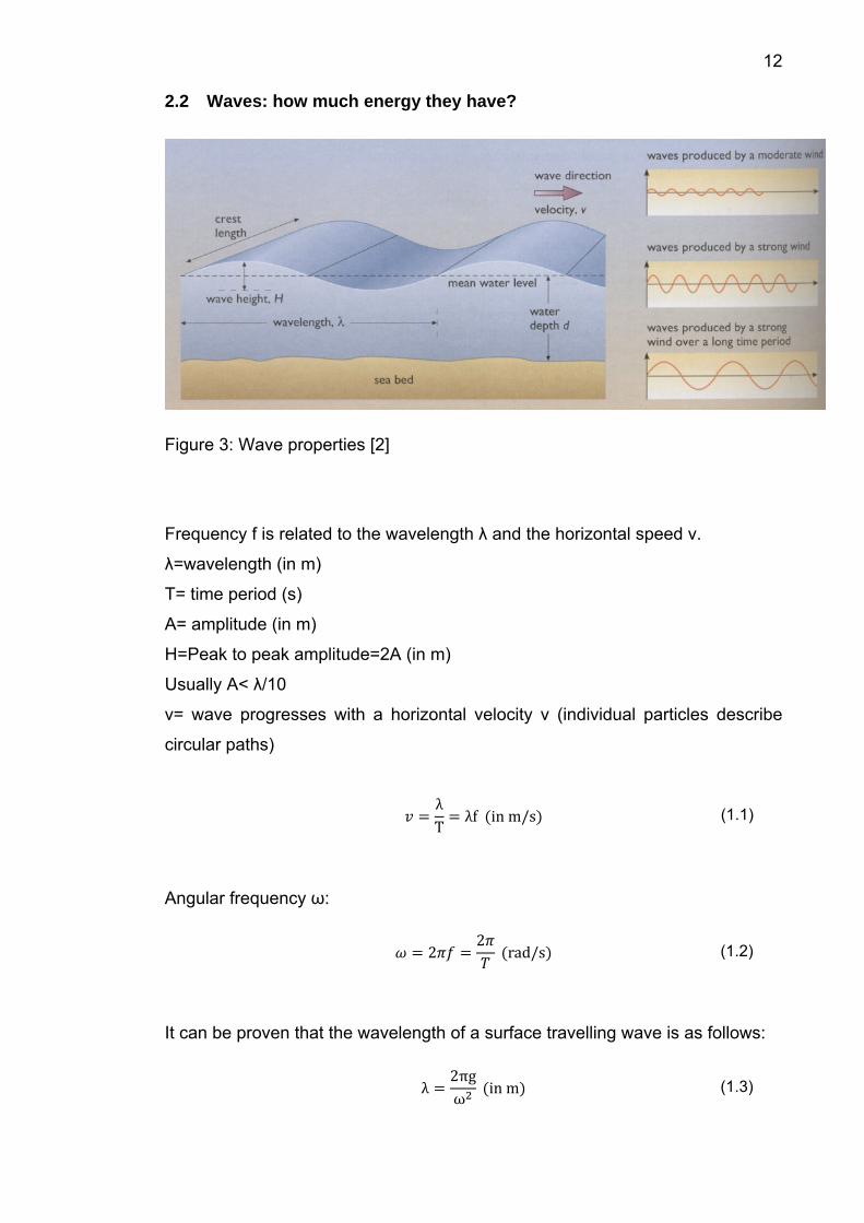
12 2.2 Waves: how much energy they have?
Figure 3: Wave properties [2]
Frequency f is related to the wavelength λ and the horizontal speed v.
λ=wavelength (in m)
T= time period (s)
A= amplitude (in m)
H=Peak to peak amplitude=2A (in m)
Usually A< λ/10
v= wave progresses with a horizontal velocity v (individual particles describe
circular paths)
λ
Tλf in m/s (1.1)
Angular frequency ω:
22
rad/s (1.2)
It can be proven that the wavelength of a surface travelling wave is as follows:
λ
2πgω
in m (1.3)

13 The last two expressions together give us:
2 λs (1.4)
With g = 9.81 m/s²
In the Atlantic ocean waves typically have periodic times of 10 seconds. This
equals a wavelength of approximately 156 meters.
• Horizontal speed.
λf
λ2
(1.5)
λf2πgω
f2πgωω 2π
gω
g2πf
gT2π
g2 λ 2
λg2
(1.6)
The velocity v is independent of the wave amplitude H.
What is the total energy in the wave? This is important to know because we
cannot extract more than maximum 50% of the energy that the wave contains.
The total energy E (caused by potential and kinetic energy) in each wavelength,
per unit width of wave crest of an individual wave is found to be (linear wave
theory):
8
J/m/λ J/mP2P (1.7)
For a certain wavelength per unit crest width:
λ8
J/m (1.8)
This is the energy per meter coast wave front length

14 λ
ω2πg
(1.9)
8
2πgω
J/m (1.10)
4
(1.11)
And
2 (1.12)
So:
116
(1.13)
The theoretical maximum power, P ideal, corresponding to the total energy con-
tent, per unit crest width, under ideal conditions (one sinus, deep water) is:
116
(1.14)
Fill in with common values:
1000
9,81
1915 (1.15)
2.3 How much energy can we extract from an ideal wave?
In reality, a wave consists of more than one sine, it is a complicated combina-
tion of waves having different wavelengths, directions and time-phase dis-
placements.
15 Mathematically it can be shown that the speed of the overall average wave mo-
tion, for random waves, is only half of the power of an individual wave. The en-
ergy content of a group of waves is transmitted at only one half of this velocity.
So the practical power extractable per meter of wave front is:
18 2
in W/m (1.16)
But even this value is not realistic. The best way to determine the overall effect
is to measure it repeatedly and use statistical data based on measured previous
performance.
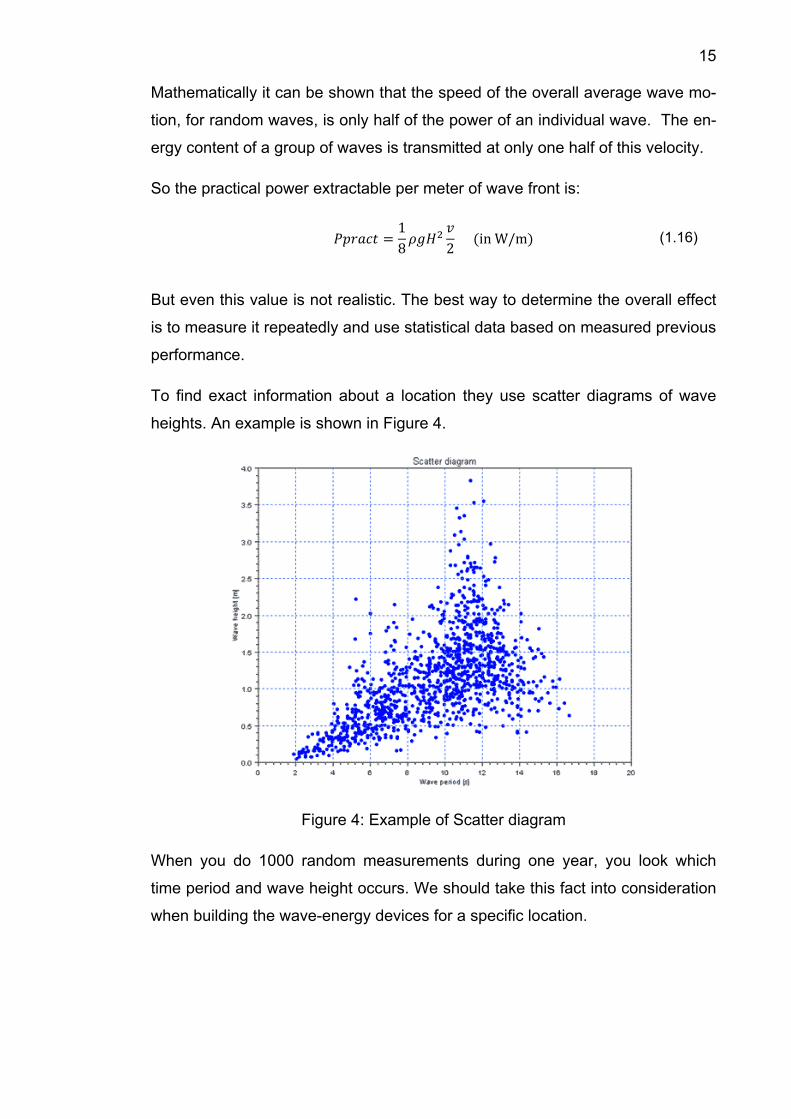
To find exact information about a location they use scatter diagrams of wave
heights. An example is shown in Figure 4.
Figure 4: Example of Scatter diagram
When you do 1000 random measurements during one year, you look which
time period and wave height occurs. We should take this fact into consideration
when building the wave-energy devices for a specific location.

16 2.4 Which part of the power can a buoy extract?
In this project (ASWEC) we use a buoy as a wave energy convertor. In our
models we use another formula. Since a buoy has a certain volume, it can only
extract power within its reach. A formula has been developed for the energy that
can be collected from a buoy:
4 2
(1.17)
This formula is used in all of our models.
2.5 Global wave energy possibilities
The theoretical potential is all wave energy there is on earth. As I mentioned
before, waves are generated by the wind and the wind energy is produced by
solar energy. So the theoretical potential is the amount of energy of the sun
that is being used for making waves.
It is logical that we cannot extract it all. The technical potential is what we are
able to extract. It takes the overall efficiency, and the available place in count.
And when we use economical potential, we look if it is a good investment in
comparison to the other energy sources. The global commercial wave-energy
potential is currently zero, only if the price drops with factor 3 it would be eco-
nomically responsible to use it. [3]
Type of potential Unit value
theoretical potential TW 14
Global theoretical potential TWh/year 18000
TW 2
Global technical potential Twhe/year 1460
Gwe 556
[3]
Considering these values some calculation can be made.
In 2005 the global electricity consumption was around 15 TW. With a total en-
ergy consumption of 131400TWh/year.

17
15 24 365 131400 /
So the technical potential is estimated on 1.1% (1460/131400) of the total elec-
trical energy production. This is not much, but all little efforts can help especially
for local consumption and remote places.
According to the world energy council, the global wave energy resource is esti-
mated to be 1-10 TW, we calculated with 2TW. The economic potential for fu-
ture devices could rise up to 2000TW (1,5%). Nowadays the economic potential
is 140-750 TWh/year (0,11% - 0,56%).
When waves move to shallower water, they lose a lot of their energy. But the
sea-bed can collect those waves and focus them in so called ‘hot spots’. Those
spots are the ideal areas for implementing our devices.
Properties of wave energy:
‐ Extractable at day – and night-time
‐ Changes during the year. In Belgium, for example, waves are bigger and
contain more energy during wintertime.
‐ Economic potential, only if the price drops with factor 3.
18 3 THE ASWEC PROJECT
ASWEC is the name of the machine that we try to develop in the project in
TAMK. ASWEC stands for ‘Aaltosorvi wave energy convertor’.
Several other students have worked or are working on this project. This means
a lot of different things have been done already. While previous tasks were
mainly theoretical, I had the luck to do the more practical part. As shown start-
ing from page 21 we started with mounting a test bench. This made us able to
do some practical measurements and compare these with previous made esti-
mations.
Thanks to a software program (see servo drive part further on), it was possible
to drive our servo motor in such a way that it simulates waves. We were able to
measure the generator output and think about how to solve the net connection
issues.
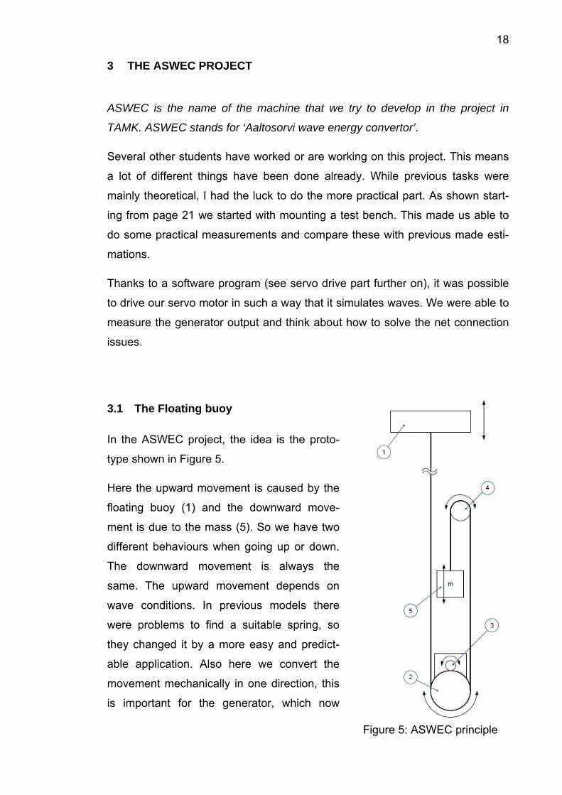
3.1 The Floating buoy
In the ASWEC project, the idea is the proto-
type shown in Figure 5.
Here the upward movement is caused by the
floating buoy (1) and the downward move-
ment is due to the mass (5). So we have two
different behaviours when going up or down.
The downward movement is always the
same. The upward movement depends on
wave conditions. In previous models there
were problems to find a suitable spring, so
they changed it by a more easy and predict-
able application. Also here we convert the
movement mechanically in one direction, this
is important for the generator, which now
Figure 5: ASWEC principle

19 turns in only one direction.
This type of convertor has the disadvantage that there is a moment in which the
speed becomes zero. This results in a voltage dip at the generator output which
is not desirable for grid connection. One of the main issues is to deal with this
problem.
20 4 THEORETICAL MODEL
The generator is simulated in a Matlab model. This model helps us make pre-
dictions about e.g. the reaction of the generator when loaded with different
loads, when driven by different speeds etc.
One of the goals of the project was to get the theoretical model as accurate as
possible. Due to this, a practical test setup was made to measure the genera-
tor’s practical parameters.
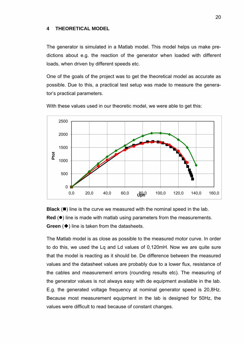
With these values used in our theoretic model, we were able to get this:
0
500
1000
1500
2000
2500
0,0 20,0 40,0 60,0 80,0 100,0 120,0 140,0 160,0
Ptot
Uph
Black ( ) line is the curve we measured with the nominal speed in the lab.
Red ( ) line is made with matlab using parameters from the measurements.
Green ( ) line is taken from the datasheets.
The Matlab model is as close as possible to the measured motor curve. In order
to do this, we used the Lq and Ld values of 0,120mH. Now we are quite sure
that the model is reacting as it should be. De difference between the measured
values and the datasheet values are probably due to a lower flux, resistance of
the cables and measurement errors (rounding results etc). The measuring of
the generator values is not always easy with de equipment available in the lab.
E.g. the generated voltage frequency at nominal generator speed is 20,8Hz.
Because most measurement equipment in the lab is designed for 50Hz, the
values were difficult to read because of constant changes.

21 5 TEST EQUIPMENT
Preliminary to my thesis, a lot of theoretical models and estimations were made.
The next step of the project is to compare the theoretical estimations with real
measurements. In order to do so, we had to make a test setup, which is shown
in Figure 6. This setup exists out of a generator, a gearbox and a motor. The
goal is to simulate the waves with the motor and compare the practical genera-
tor voltage with the theoretic model.
Figure 6: Test equipment
Servomotor Gearbox 6/1 Permanent Magnet
Generator

22 5.1 Permanent Magnet Generator
Main characteristics:
nn nmax fs Pn In UY
rpm rpm Hz kW A V
250 500 20,8 2,0 5,0 250
The most important part of the setup is the Permanent Magnet Generator. The
generator generates an AC voltage. This voltage will change when the genera-
tor speed changes.

23 5.1.1 Theoretical generator characteristics
The manufacturer of the generator gave us following properties of the genera-
tor. The full generator datasheet can be found in Annex 1.
There are different characteristics for passive and active loading. A passive load
is a load acting as a resistor. An active load is a load which behaves as a non-
linear resistor e.g. capacitor or inductance.
Passive loading:

24 Active loading:
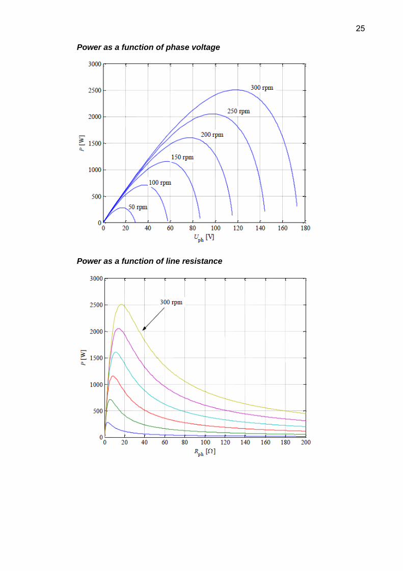
25 Power as a function of phase voltage
Power as a function of line resistance

26 5.1.2 Practical generator characteristics
Out of the datasheet of the manufacturer (Annex 1) we could find some pa-
rameters. To be sure we are using the correct parameters; we measured and
calculated them from our generator. The flux can vary when the Permanent
Magnets are getting older.
Used Given by manufacturer Note
RRs 2,05 1,6
Used value is the value of WARM
engine
Ld 0,12 0,12
Found by testing different values
(fits best)
Lq 0,12 0,12
Found by testing different values
(fits best)
Flux 1,35 1,56* Calculated from the no load test
* flux calculated out of datasheet parameters
Resistance: measured with ohm meter and calculated for 1 phase (Calculation
is needed since motor is switched in star-connection)
Ld & Lq: found by comparing several values in Matlab, chosen the best fitting
one.
Ld is the direct axis inductance and Lq the quadrature axis inductance. These
are fundamental inductances of the generator since a permanent magnet gene-
rator is usually presented with two axis circuits.
Flux: found by measuring the induced line voltage, then took the average of the
three phases, converted it to phase voltage (= Epm) and peak phase voltage
(amplitude). Flux is calculated out of this.
s
PM
s
PMPMPMsPM 2
2ˆˆf
EEΨΨE⋅⋅
⋅==⇒⋅=
πωω
The flux 1,35Wb is found at constant speed. For changing speed measure-
ments the best fitting flux is 1,38Wb.

27 5.1.3 Comparison between theoretical and practical values
To be sure the generator is reacting as it should be; we reproduced the meas-
urements found in the generator datasheet and compared them with the theo-
retical values. Since this was not the subject of this thesis, results of those
measurements are not written down here. Anyone who is interested in these
results can find them in the thesis of Henri Toijala.
[Henri Toijala, Aaltovoimalaitteiston PM generaattorin ja tasasuuntauksen mal-
lintaminen ja testaus, Tampere University of Applied Sciences, 2011]
5.2 Servo Motor
Characteristics:
nn Mn Mk
rpm Nm Nm
3000 18 23,4
In a real sea-wave situation, the generator is driven by waves. This means the
buoy goes up and down and stands still for a short moment when changing di-
rection. The generator axis stands still as well. To simulate this, the servomotor
is controlled by a computer program, which enables the motor to act like real
waves. The program is made by another student. It is possible to load an Excel-
file with wave data in the program. This way, different waves (high, low,…) can
be simulated. A print screen of the program is shown in Figure 7.

28
Figure 7: Print screen of the servomotor control program
5.3 Gear
The gearbox is used because the nominal generator speed is 250rpm while the
servomotors’ nominal speed is 3000rpm. The ratio of the gearbox is 6/1.
Characteristics:
Manufacturer: SEW-EURODRIVE
Model: R47 AD2
n1: 1400 rpm
n2: 233 rpm

29 6 INDUCED VOLTAGE SHAPING
To inject the generated energy into the grid, the power has to be smooth
enough. This means that the unwanted oscillations are minimized. The goal is a
perfect sinus with a frequency of 50Hz. The first step is rectifying the voltage,
and then we try to keep this DC voltage as constant as possible, even if the
generated voltage varies. The next step is to produce a sine wave of 50Hz to
inject the generated energy in the grid. These three steps are explained hereaf-
ter.
Theoretically the DC link and net connection can be schematized as follows in
Figure 8:
Figure 8: DC link and net connection
The power available for extraction varies dramatically depending on the sea-
state, leading to a high ratio of peak powers to the long term average value. The
end requirement of any grid-connected electrical generation system is a positive
power-flow of sinusoidal AC at the appropriate line frequency (in our case
50Hz). Power flow should be substantially constant over a time period of min-
utes or more, so as to provide a stable (and saleable) contribution of energy to
the grid.
A conventional strategy for conditioning the output of a variable frequency gen-
erator is controlled rectification of its output. This provides a steady DC-link
voltage, which is then used to feed the main grid via a 3-phase inverter bridge.

30 6.1 Step 1: diode bridge
Figure 9: Basic diode bridge
The first step is rectifying the voltage. A 3-phase diode bridge is used for this
purpose. A basic diode bridge is shown in Figure 9. As we can see on Figure
10, the generated voltage has dips. This is caused by the tops and bottoms of
the waves. That moment, the buoy does not move, so the induced voltage is
zero.
2.5 3 3.5 4 4.5-400
-300
-200
-100
0
100
200
300
400Jännite (V)
Figure 10: Generated voltage

31
2.5 3 3.5 4 4.50
2
4
6
8
10
12
14
16
18
20Teho (kW)
Figure 11: Rectified generator voltage
After rectification, the voltage dips are still visible as shown in Figure 11. Due to
grid connection, this problem has to be solved. Some possibilities are explained
in 6.2.
6.1.1 Losses in the bridge of diodes
To measure the practical losses in the diode bridge, we compare the ingoing
power with the outgoing power. The differences between both are the losses.
The efficiency can be easily calculated by dividing the outgoing power by the
incoming power.
The measurements learn us that the diode bridge efficiency at peak generated
power is 0,93. At other speeds and powers, the efficiency is between 0,90 and
0,93.
For example:
At the nominal speed of 250rpm, the generator’s generated peak power is
1709W. After the bridge of diodes, we have left 1597,5W. So, there is a loss of
111,6W. Out of this we can calculate the efficiency, which is 0,93 in this case.

32 6.2 Step 2: DC link voltage
When this voltage is rectified, the voltage-dips are still visible. Before we trans-
form the DC-voltage in to a 50Hz AC voltage which is suitable for the grid, we
want to make the DC-voltage as smooth as possible.
6.2.1 Super capacitor
One of the ways to smoothen the DC-voltage is to implement a super capacitor.
Theoretically, this is a good solution, but there are some practical disadvan-
tages. The biggest issue is that the estimated life of the capacitor is too short,
which results in an increased maintenance level and higher costs, especially if
this is implemented in off-shore applications. If we use the super capacitor only
in extreme wave conditions, we can extend the lifetime of the capacitor. Another
solution is to mount the capacitor at the coastline, which facilitates the mainte-
nance.
In our project we try to avoid the super capacitor because of the expensiveness
and sensitivity.
6.2.2 DC-DC converter: Boost convertor
Another way to smoothen the DC side can be a boost convertor. A basic boost
converter is shown in Figure 12. As said, the main problem was the voltage-dips
in the rectified voltage. As the name implies, the output voltage of a boost con-
vertor is always greater than the input voltage. So, if we can use the boost con-
vertor to increase the voltage in the dip points, this could result in a more
smooth voltage. The boost-converter is a type of DC-DC converter. The output
voltage of DC-DC converters can be adju ted by changing the duty cycle D. s
Here, the switches are treated as being ideal, and the losses in the inductive
and the capacitive elements are neglected. Such losses can limit the opera-
tional capacity of the converter. The DC input voltage to the converters is as-

33 sumed to have zero internal impedance. In our case, the voltage is generated
by the generator and will have an internal impedance, one of the difficulties of
this subject is the question how we can use this impedance as part of the con-
verter.
Basic principle
When the switch is on, the diode is reversed biased, thus isolating the output
stage. The input supplies energy to the inductor. When the switch is off, the
output stage receives energy from the inductor as well as the input. In the
steady-state analysis presented here, the output filter capacitor is assumed to
be very large to ensure a constant output voltage vo(t) ≅ Vo.
Continuous-conducting mode
Figure 13 shows the steady-state waveforms for this mode of conduction where
the inductor current flows continuously [iL(t) > 0]. Since in steady state the time
integral of the inductor voltage over one time period must be zero,
Vdton + (Vd – V0)toff = 0
Figure 12: Step-up DC-DC convertor [4]

34
Figure 13: Continuous-conducting mode: (a) switch on; (b) switch off. [4]
Dividing both sides by Ts and rearranging terms yields:
11
(2.1)
Assuming a lossless circuit, Pd = P0,
VdId = V0I0 (2.2)
And
1 (2.3)
Boundary between continuous and discontinuous conduction Figure 14a shows the waveforms at the edge of continuous conduction. By
definition, in this mode iL goes to zero at the end of the off interval. The average
value of the inductor current at this boundary is
12 , (2.4)

35
21
(2.5)
2
1 (2.6)
Figure 14: Step-up DC-DC converter at the boundary of continuous-
discontinuous conduction. [4]
Recognizing that in a step-up converter the inductor current and the input cur-
rent are the same (id = iL) and using Eq.(2.3) and (2.6), we find that the average
output current at the edge of continuous conduction is
2
1 ² (2.7)
Most applications in which a step-up converter is used require that V0 be kept
constant. Therefore, with V0 constant, I0B are plotted in Figure 14b as a function
of duty ratio D. Keeping V0 constant and varying the duty ratio imply that the
input voltage is varying.
Figure 14b shows that ILB reaches a maximum value at D = 0,5:
, 8 (2.8)
Also, I0B has its maximum at D = = 0,333:
,
227
0,074 (2.9)
In terms of their maximum va es an be expressed as lu , ILB and I0B c
4 1 , (2.10)
36 And
274
1 ² , (2.11)
Figure 14b shows that for a given D, with constant V0, if the average load cur-
rent drops below IOB (and, hence, the average inductor current below ILB), the
current conduction will become discontinuous.
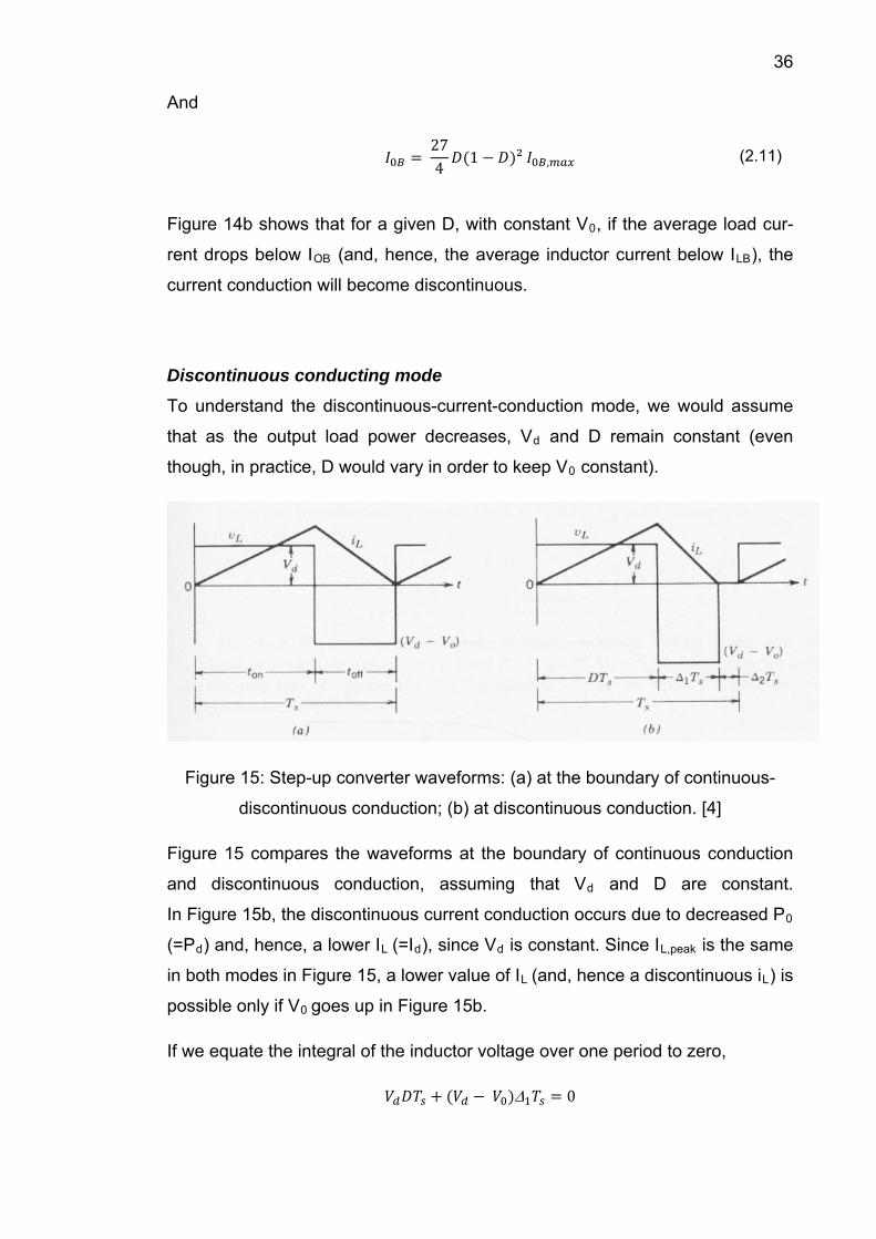
Discontinuous conducting mode
To understand the discontinuous-current-conduction mode, we would assume
that as the output load power decreases, Vd and D remain constant (even
though, in practice, D would vary in order to keep V0 constant).
Figure 15: Step-up converter waveforms: (a) at the boundary of continuous-
discontinuous conduction; (b) at discontinuous conduction. [4]
Figure 15 compares the waveforms at the boundary of continuous conduction
and discontinuous conduction, assuming that Vd and D are constant.
In Figure 15b, the discontinuous current conduction occurs due to decreased P0
(=Pd) and, hence, a lower IL (=Id), since Vd is constant. Since IL,peak is the same
in both modes in Figure 15, a lower value of IL (and, hence a discontinuous iL) is
possible only if V0 goes up in Figure 15b.
If we equate the integral of the inductor voltage over one period to zero,
Δ 0

37 Δ
Δ (2.12)
And
ΔΔ
(2.13)
From Figure 15b, the average input current, which is also equal to the inductor
current, is
2Δ (2.14)
Using equation (2.13) in the foregoing equation yields
2
Δ (2.15)
In practice, since V0 is held constant and D varies in response to the variation in
Vd, it is more useful to obtain the required duty ratio D as a function of load cur-
rent for various values of V0/Vd. By using Eqs. (2.12), (2.15) and (2.9), we de-
termine that
427
1,
(2.16)
In Figure 16, D is plotted as a function of I0/I0B,max for various values of Vd/V0.
The boundary between continuous and discontinuous conduction is shown by
the dashed curve.
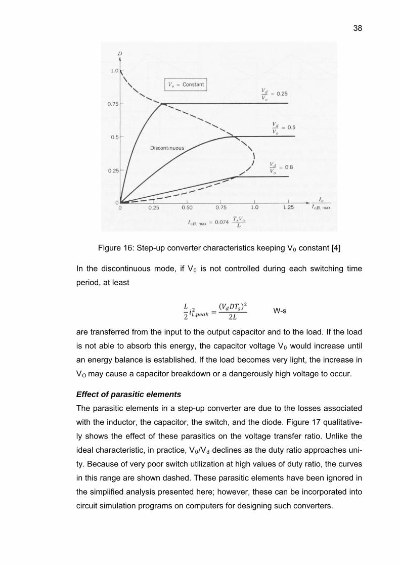
38
Figure 16: Step-up converter characteristics keeping V0 constant [4]
In the discontinuous mode, if V0 is not controlled during each switching time
period, at least
2 ,²
2W-s
are transferred from the input to the output capacitor and to the load. If the load
is not able to absorb this energy, the capacitor voltage V0 would increase until
an energy balance is established. If the load becomes very light, the increase in
VO may cause a capacitor breakdown or a dangerously high voltage to occur.
Effect of parasitic elements
The parasitic elements in a step-up converter are due to the losses associated
with the inductor, the capacitor, the switch, and the diode. Figure 17 qualitative-
ly shows the effect of these parasitics on the voltage transfer ratio. Unlike the
ideal characteristic, in practice, V0/Vd declines as the duty ratio approaches uni-
ty. Because of very poor switch utilization at high values of duty ratio, the curves
in this range are shown dashed. These parasitic elements have been ignored in
the simplified analysis presented here; however, these can be incorporated into
circuit simulation programs on computers for designing such converters.

39
Figure 17: Effect of parasitic elements on voltage conversion ratio (step-up con-
verter) [4]
Output voltage ripple
The peak-to-peak ripple in the output voltage can be calculated by considering
the wave-forms shown in Figure 18 for a continuous mode of operation. Assum-
ing that all the ripple current component of the diode current iD flows through
the capacitor and its average value flows through the load resistor, the shaded
area in Figure 18 represents charge ΔQ. Therefore, the peak-peak voltage rip-
ple is given by
Δ Δ (assuming stant output current) a con
Δ
(2.17)
τ (where τ = RC time constant) (2.18)

40 A similar analysis can be performed for the discontinuous mode of conduction.
Figure 18: Step-up converter output voltage ripple [4]
Boost Converter Control
One of the methods for controlling the output voltage employs switching at a
constant frequency (hence, a constant switching time period Ts = ton + toff) and
adjusting the on duration of the switch to control the average output voltage. In
this method, called pulse-width modulation (PWM) switching, the switch duty
ratio D, which is defined as the ratio of the on duration to the switching time
period, is varied.
Another control method is more general, where both the switching frequency
(and hence the time period) and the duration of the switch are varied. This
method is used only in DC-DC converters utilizing force-commutated thyristors.
In our PSpice simulation control, we use the first method with constant
switching frequency.

41
Figure 19: Pulse-width modulator: (a) block diagram; (b) comparator signals [4]
In the PWM switching at a constant frequency, the switch control signal, which
controls the state (on or off) of the swith, is generated by comparing a signal-
level control voltage vcontrol with a repetitive waveform as shown in Figure 19 (a)
and (b). The control voltage signal generally is obtained by amplifying the error,
or the difference between the actual output voltage and its desired value. The
frequency for the repetetive waveform with a constant peak, which is shown to
be a sawtooth, establishes the switching frequency. This frequency is kept
constant in a PWM control and is chosen to be in a 1kHz to 8kHz range in our
case. When the amplified error signal, which varies very slowly with time
relative tot the switching frequency, is greater than the sawtooth waveform, the
switch control signal becomes high, causing the switch to turn on. Otherwise,
the switch is off. In terms of vcontro l and the peak of the sawtooth waveform Vst
in Figure 19, the switch duty ratio can be expressed as
The DC-DC converters can have two distinct modes of operation: (1)
continuous current conduction and (2) discontinuous current conduction. In
practice, a converter may operate in both modes, which have significantly

42 different characteristics as shown in 6.2.2. Therefore, a converter and its control
should be designed based on both modes of operation. [4]
6.3 Step 1 + 2: Unidirectional boost rectifier
This information is taken from a wave energy conversion example with a linear
generator. Because our voltage and current have similar shapes, we can use
the same technology.
6.3.1 Unidirectional rectifier
If the mechanical power take-off system can achieve the desired response to
input waves without the need for bi-directional power flow with the generator, a
unidirectional rectifier topology can potentially be used to afford cost savings in
the power electronics. For machines with sufficiently high intrinsic power factor,
such as an air-cored tubular linear generator a unidirectional Power Factor
Converter stage can achieve the desired current shaping.
The boost topology shown in Figure 20 has been proposed and demonstrated
by Ran et al. [5]; where each generator coil is connected to its own boost con-
verter feeding an intermediate DC-link. We can use a single boost converter per
phase, operating directly into a high voltage DC-link.
The topology consists of an uncontrolled rectification stage, followed by a boost
mode Power Factor Correction circuit, where the generator’s phase inductance
is used as the boost inductor, placed before the input diodes.
Figure 20: Unidirectional boost rectifier [6]
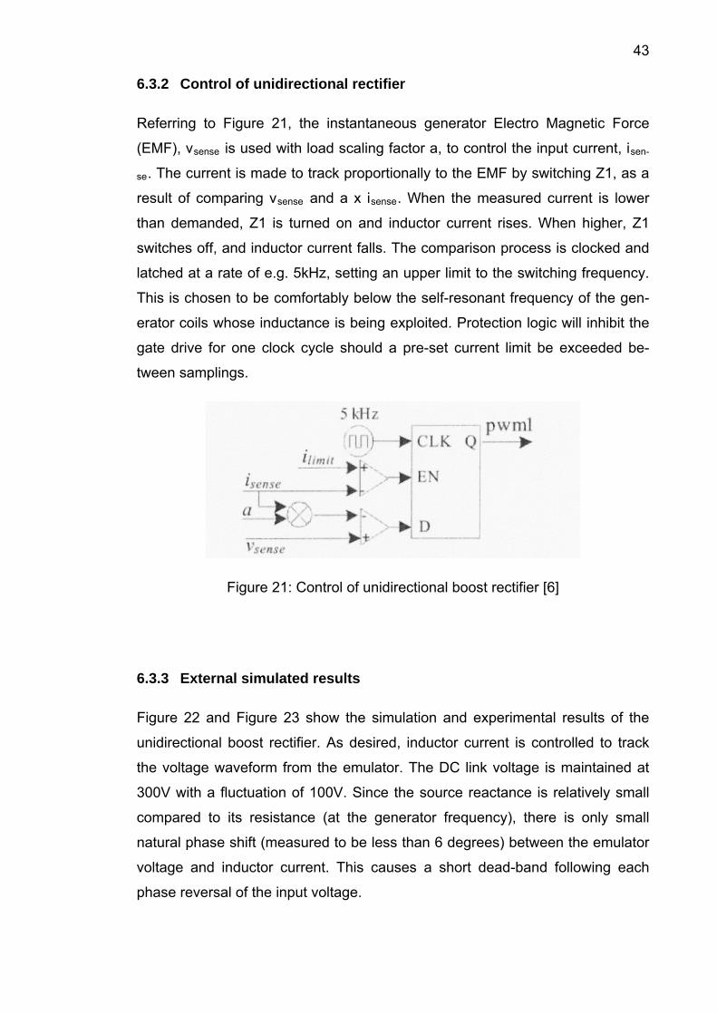
43 6.3.2 Control of unidirectional rectifier
Referring to Figure 21, the instantaneous generator Electro Magnetic Force
(EMF), vsense is used with load scaling factor a, to control the input current, isen-
se. The current is made to track proportionally to the EMF by switching Z1, as a
result of comparing vsense and a x isense. When the measured current is lower
than demanded, Z1 is turned on and inductor current rises. When higher, Z1
switches off, and inductor current falls. The comparison process is clocked and
latched at a rate of e.g. 5kHz, setting an upper limit to the switching frequency.
This is chosen to be comfortably below the self-resonant frequency of the gen-
erator coils whose inductance is being exploited. Protection logic will inhibit the
gate drive for one clock cycle should a pre-set current limit be exceeded be-
tween samplings.
Figure 21: Control of unidirectional boost rectifier [6]
6.3.3 External simulated results
Figure 22 and Figure 23 show the simulation and experimental results of the
unidirectional boost rectifier. As desired, inductor current is controlled to track
the voltage waveform from the emulator. The DC link voltage is maintained at
300V with a fluctuation of 100V. Since the source reactance is relatively small
compared to its resistance (at the generator frequency), there is only small
natural phase shift (measured to be less than 6 degrees) between the emulator
voltage and inductor current. This causes a short dead-band following each
phase reversal of the input voltage.

44
Figure 22: PSpice results for the emulator voltage, coil current and output vol-
tage for the unidirectional rectifier [6]
Figure 23: Experimental results for the emulator voltage, coil current and output
voltage for unidirectional rectifier [6]
6.3.4 Losses
One system design challenge is to balance the trade-off between system effi-
ciency and maximum power extraction. In conventional generation, system effi-
ciency is a critical concern due to the cost of wasted fuel. However, in renew-
able generation, the “fuel” is free, skewing the economics to focus more on
capital and operating costs for a given output rating. Due to this, it is possible to
choose to operate with high losses in order to increase power output for a given
size generator. [6]
45 6.3.5 Test equipment: theoretical boost converter parameters
The externally simulated results indicate that we should be able to get our volt-
age much better with the boost converter. To simulate this for our equipment,
we need a realistic value of boost converter’s L.
Out of Eq. (2.8) and our equipment parameters we are able to define the L
value which should be used in our boost converter simulation.
, 8
8 ,
With
ILB, max= 8A
Ts= 1/f with f = 10000Hz
Vo= 326V
Which leads to
110000 . 326
8.8
0,50938

46
6.4 Step 3: DC Transport basics
Instead of thinking in the traditional way and transport the energy in AC, the
choice of DC transportation has its benefits. Especially; because we already
use a boost converter which should make a smooth DC-voltage. This means
that we are converting the energy back to AC only when the energy is on land
already. If we try to use a boost converter to get a smoother DC voltage, if cor-
rectly designed, we might be able to use this output voltage directly as High Vol-
tage Direct Current transport line. An example of DC transportation is shown in
Figure 24.
Figure 24: DC topology
Using a DC transport line has its benefits, especially for longer distances e.g. at
sea. The biggest benefit is the absence of a third cable. This means a lower
copper price, or, if used the same amount of copper for 2 lines: less losses. In
some cases, there is only one DC line used, the seabed acts as the 2nd line. If
so, the copper price is even lower.
6.4.1 Common DC bridge
As shown on Figure 25, one option can be that the DC transport line is used to
couple different wave energy conversion devices. In this case the fluctuation of
the DC voltage might be minimalized. Another advantage is that we need only
one HVDC cable for several devices.

47
Figure 25: DC connection + transportation
6.4.2 Main HVDC advantage
The advantage of HVDC is that long distance transmission is more efficient as
there is no need to charge the capacitance of a transmission line with the alter-
nating voltage.
HVDC has a number of properties which make it different from AC-
transmission. The most important are:
- The two stations can be connected to networks that are not synchronized or
do not even have the same frequency.
- Power can be transmitted over very long distances without compensation for
the reactive power. Reactive power is power that does not add to the transmit-
ted power, but is a by-product at AC-transmission as the line or cable capaci-

48 tances have to be charged 50 or 60 times per second. As HVDC has a constant
voltage it does not generate reactive power.
- Only two conductors are needed (or even one conductor if the ground or the
sea is used as return) for HVDC compared to three conductors for alternating
current. [7]
6.4.3 Conclusion
A DC transporting line can have benefits for the wave energy, but many pa-
rameters influence the choice. First we have to know the distance, power, etc.
before a good decision can be made.

49 6.5 Step 4: Three phase inverter
6.5.1 PWM - converter
In applications such as uninterruptible AC power supplies and AC motor drives,
three-phase inverters are commonly used to supply three-phase loads. It is
possible to supply a three-phase load by means of three separate single-phase
inverters, where each inverter produces an output displaced by 120° (of the
fundamental frequency) with respect to each other. Though this arrangement
may be preferable under certain conditions, it requires either a three-phase out-
put transformer or separate access to each of the three phases of the load. In
practice, such access is generally not available. Moreover, it requires 12
switches.
The most frequently used three-phase inverter circuit consists of three legs, one
for each phase, as shown in Figure 26. The output of each leg, for example vAN
(with respect to the negative DC bus), depends only on Vd and the switch
status; the output voltage is independent of the output load current since one of
the two switches in a leg is always on at any instant. Here, we ignore the blank-
ing time required in practical circuits by assuming the switches to be ideal.
Therefore, the inverter output voltage is independent of the direction of the load
current.
Most frequency converters are using a PWM control, which is obtained by using
a sawtooth voltage and a control voltage. Its working is not discussed here.
Figure 26: a three-phase converter [4]

50 6.5.2 Solution when incoming voltage varies
Because it is not easy to get a perfect smooth DC-voltage in the DC-link, the
converter which transforms the DC into 50Hz AC can have a slightly variable
voltage. To deal with this, we can use a ‘Feed Forward’ PWM converter. This is
a PWM converter which can directly change the duty cycle. In this way, the
output voltage stays the same, when the input voltage varies. Voltage Feed
Forward regulation is shown in Figure 27.
This technique is realized by adding the input voltage to the PWM-control. The
only difference with the normal PWM-converter is that now the amplitude of the
sawtooth voltage VT is not constant, but changes proportionally with the input
voltage.
Figure 27: Voltage 'Feed-Forward' PWM regulation [8]
Since we are expecting to have a not perfect smooth DC-link, this can be very
useful.

51 7 BOOST CONVERTER SIMULATION
As said in 6.3.3, others were able to simulate a boost converter on a voltage
which has the same shape as in our case. We know they have it, and it might
be a solution for our case. But, in the found external result, nothing was said
about the transmitted power and eventually used capacitors. A simulation suit-
able for our case has to be made to ensure this.
Note: In the simulation schemes colored pins are used to show where meas-
urements are taken. The colours of the pins do not match with the colours of the
lines in the result graphs.
7.1 PSpice boost converter topology
Both Matlab and PSpice simulations are commonly used. Because a working
boost converter simulation in PSpice was available, I tried to work with this.
Figure 28 shows the first made boost converter simulation topology. There are
four main components. The generator, DC-bridge, boost converter, and the
load.
Figure 28: Boost Converter Topology
The model shown in Figure 28 had a lot of errors, because of undefined rea-
sons the model did not recognize the switching part of the boost converter.
Many alternatives were tried, but the result was always the same. The model
was not running at all, or it was running with a non-active boost converter.

52 7.2 Basic boost converter – DC input
Since the first model was not working, another model was made; starting from a
different working boost converter model. The difference here is the boost con-
verter which is build out of alternative parts. Comparison between Figure 28 and
Figure 29 show this difference.
Figure 29: Basic boost converter
To test if this converter is working, a 200V DC voltage is placed at the input.
The simulation result is given in Figure 30. As shown, the output voltage varies
around the 400V DC, while the input voltage is 200V DC. One leads to the con-
clusion this boost converter is working.
In Figure 31 a zoom of the result is given. As shown, the switching moments of
the boost converter are clearly detected in the output voltage. The output volt-
age varies approximately 50V.

53
Figure 30: Basic DC boost result
Figure 31: Zoom of basic DC boost result
Figure 32: Close up of basic DC boost result
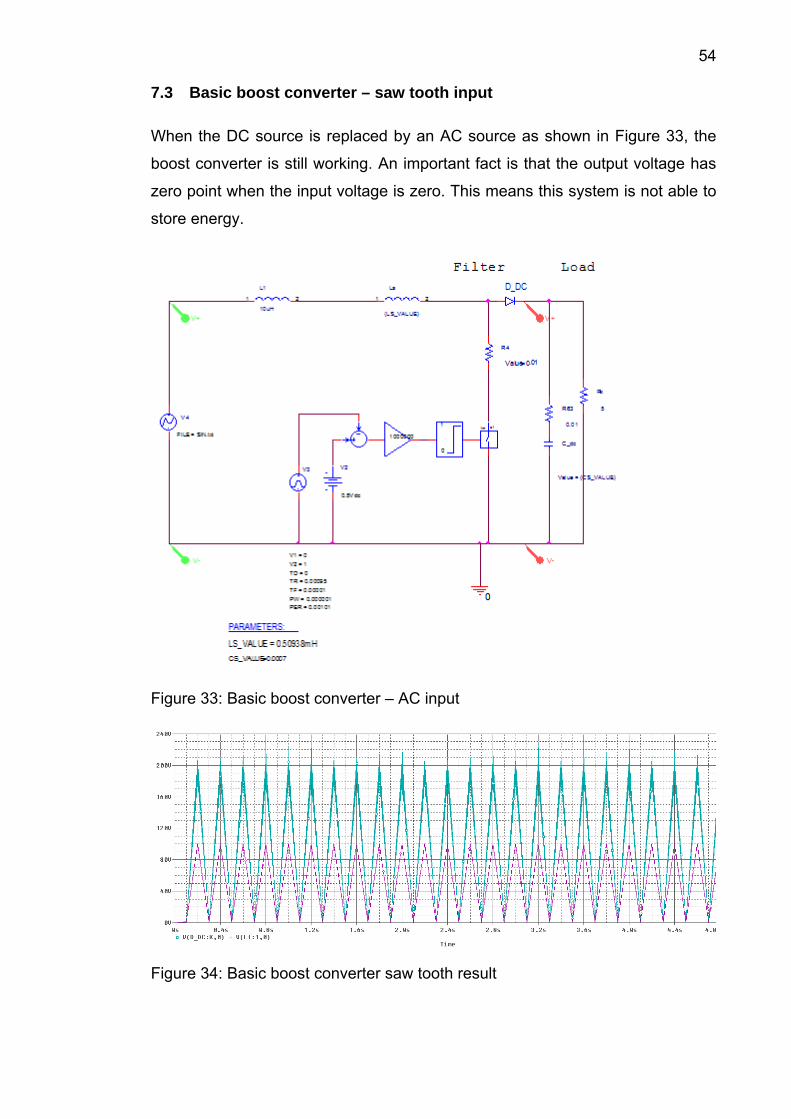
54 7.3 Basic boost converter – saw tooth input
When the DC source is replaced by an AC source as shown in Figure 33, the
boost converter is still working. An important fact is that the output voltage has
zero point when the input voltage is zero. This means this system is not able to
store energy.
Figure 33: Basic boost converter – AC input
Figure 34: Basic boost converter saw tooth result

55
Figure 35: Close up of saw tooth result
7.4 Basic boost convertor – 1 phase wave form input
As shown on Figure 36, the boost converter is still doing its job, but the zero
points are still present.
Figure 36: Basic boost converter - wave form input

56
Figure 37: Close up from wave form result
7.5 Basic boost converter – 1 phase rectified input
By adding a one phase diode bridge as shown in Figure 38, the input voltage is
now rectified.
Figure 38: Basic boost converter - one phase rectified input
The output result is shown in Figure 39. Compared with Figure 36, the average
output power is increased.

57
Figure 39: 1 phase rectified output
Figure 40: Close up of phase rectified result
7.6 Three-phase boost converter input
Since we know the boost converter is working, we can now try to simulate again
with the generator. This part is copied from the first –not working- simulation.
Generator parameters are set on L=120mH and R=2,05Ω for each line. A 3-
phase bridge rectifies the induced voltage.

58
Figure 41: 3-phase basic boost converter
Figure 42: 3-phase boost converter result

59
Figure 43: Close up of 3 phase boost converter result
Figure 44: 3-phase boost converter result zoom
As we look closer to the output voltage, we see the output voltage is still very
close to zero on the crucial moment. The boost converter simply has no voltage
to boost.
Trying to avoid this, a capacitor was added.

60
Figure 45: 3-phase boost converter with DC capacitor
Figure 46: 3-phase boost converter with DC-capacitor result
Another option was placing a capacitor at the load side of the boost converter,
as shown in Figure 47.

61
Figure 47: 3-phase basic boost converter with extra C at load side
Figure 48: 3-phase boost converter with extra C at load side - result
As shown in Figure 48, the output voltage is now more constant, but still very
low.
62 7.7 Optimizing simulation Load value
Previous simulations showed the influence of the parameters is not that big.
Only one parameter is left, the load value. To calculate the optimal load we can
use a formula from wave energy converters with linear generators. Knowing the
components of the lumped circuit the active power in the load can be calcu-
lated:
² ² (3.1)
With
Pl = output power (W)
E = induced voltage (no load)
RRl = Load resistance
RgR = Generator resistance
Xs = 2.π.f.L with L = generator coil inductance 120mH
Xl = assumed zero
The active output power of a generator depends on the induced emf, the syn-
chronous reactance, the armature winding resistance and the load. The induced
emf varies with the translator speed (which we take constant 200rpm in this ex-
ample) and the output power will thus vary as the translator changes speed dur-
ing a wave period. By changing the load the output power for a given translator
speed can also change. By varying the load, the damping of the generator can
be varied. This can be used as control strategy to control the power absorbed
by the Wave Energy Converter. [1]

63 Since we want extract maximum power out of the generator, the optimal load
has to be found using (3.1). We assume a constant induced voltage of 111,8V.
Rload (Ω) Rgen (Ω) Xs (Ω) Xl (Ω) E (V) Pphase (W) 3*Pphase (W)
1 2,05 12,59 0 111,8 74,5 223,45 2,05 12,59 0 111,8 300,1 900,36 2,05 12,59 0 111,8 335,8 1007,37 2,05 12,59 0 111,8 363,9 1091,68 2,05 12,59 0 111,8 385,3 1155,89 2,05 12,59 0 111,8 400,8 1202,510 2,05 12,59 0 111,8 411,5 1234,511 2,05 12,59 0 111,8 418,1 1254,3
12 2,05 12,59 0 111,8 421,4 1264,2
13 2,05 12,59 0 111,8 422,0 1266,0
14 2,05 12,59 0 111,8 420,5 1261,515 2,05 12,59 0 111,8 417,3 1252,016 2,05 12,59 0 111,8 412,9 1238,717 2,05 12,59 0 111,8 407,5 1222,518 2,05 12,59 0 111,8 401,4 1204,119 2,05 12,59 0 111,8 394,7 1184,2
20 2,05 12,59 0 111,8 387,7 1163,2
Out of the calculations we see the highest output power is with a load of 13Ω.
Using this value in a simulation with constant input voltage, we should get a to-
tal output power of 1266W.
This is the output power of a load directly connected to a generator rotating at
constant speed. If we replace the generator and the diode bridge by a DC-
source, the value of this source can be calculated:
1,35 . √3 . (3.2)
1,35 . √3 . 11
261,42
1,8
The load Rdc in a DC-simulation is calculate d
3.² ²
(3.3)

64
.²
3. ² (3.4)
261,42²8²
13.3.111,
23,69Ω
Optimized load scheme is shown in Figure 49.
Figure 49: Optimized load scheme
65
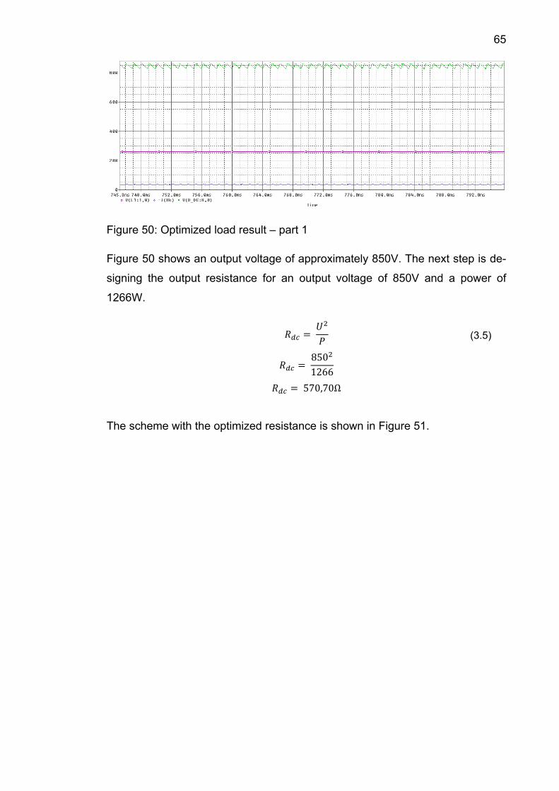
Figure 50: Optimized load result – part 1
Figure 50 shows an output voltage of approximately 850V. The next step is de-
signing the output resistance for an output voltage of 850V and a power of
1266W.
850
(3.5)
1266
570,70Ω
The scheme with the optimized resistance is shown in Figure 51.

66
Figure 51: Scheme with optimized resistance
Figure 52: Optimized load result – part 2

67
Figure 53: Optimized load result, zoom in on current
Figure 52 and Figure 53 show the result of the simulation with the optimized
load resistance of 570,69Ω. An output voltage of approximately 850V and an
output current of approximately 1,5A lead to an output power of approximately
1250W, which is close to the calculated value of 1266W.
Important is that we had to adjust the duty cycle of the boost converter by
changing the control voltage from 0,5V to 0,1V manually to get the simulation
running correctly. This proves the need of a good control which should do this
automatically.
7.8 3-phase boost & non-boost comparison
To see the effect of the boost converter in the three phase system, a compari-
son is made here.
7.8.1 3-phase without boost
3-phase without boost converter scheme is shown in Figure 54.

68
Figure 54: 3-phase no boost converter scheme
This leads to
Figure 55: 3-phase no boost converter result
69
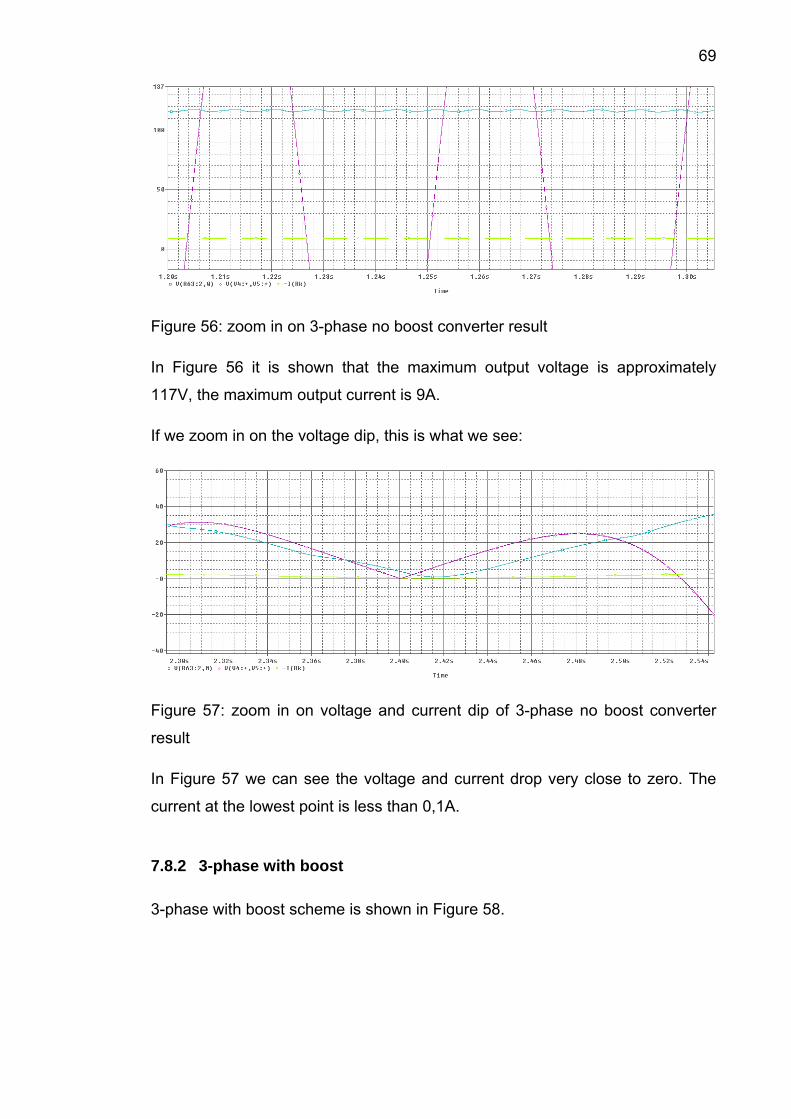
Figure 56: zoom in on 3-phase no boost converter result
In Figure 56 it is shown that the maximum output voltage is approximately
117V, the maximum output current is 9A.
If we zoom in on the voltage dip, this is what we see:
Figure 57: zoom in on voltage and current dip of 3-phase no boost converter
result
In Figure 57 we can see the voltage and current drop very close to zero. The
current at the lowest point is less than 0,1A.
7.8.2 3-phase with boost
3-phase with boost scheme is shown in Figure 58.

70
Figure 58: 3-phase with boost converter scheme
This leads to
Figure 59: 3-phase with boost converter result
Figure 60: zoom in on 3-phase with boost converter result
As we can see in Figure 60, there is a maximum output voltage of approximate-
ly 62V. The output current is 5A.

71 If we zoom in on the voltage dip, this is what we see:
Figure 61: zoom in on voltage and current dip of 3-phase with boost converter
result
Figure 61 shows the output voltage drops to 18V, and the output currents’ low-
est point is 1,2A.
7.8.3 Comparison
Both results are listed in following table.
NO boost With boost
Max. voltage 117V 62V
Max. current 9A 5A
Min. voltage (dip) 2V 18V
Min. current (dip) 0,1A 1,2A
It is clear that the voltage and current drop without the boost converter is lower
than with the boost converter. The maximum voltage and current without the
boost converter is higher, this is logic, because the boost converter stores ener-
gy, so less energy is at the output with a boost converter.
The main conclusion we can make is that the boost converter is working and
the dip is not as low as before.

72 7.9 Higher boost switching frequency
All previous simulations are made with a boost switching frequency of 1 kHz. In
our calculation of the L value of the boost converter in 6.3.5 we used a frequen-
cy of 10 kHz. A simulation using this frequency might give better results.
Figure 62: 3-phase with 10 kHz boost frequency
As shown in Figure 62 nothing changes in the scheme. Only the boost con-
verter parameters shown in Figure 63 are adjusted.
Figure 63: Boost converter parameters
73
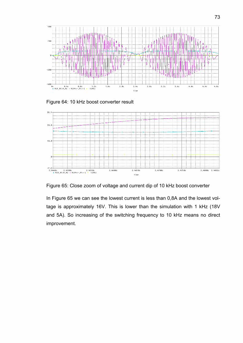
Figure 64: 10 kHz boost converter result
Figure 65: Close zoom of voltage and current dip of 10 kHz boost converter
In Figure 65 we can see the lowest current is less than 0,8A and the lowest vol-
tage is approximately 16V. This is lower than the simulation with 1 kHz (18V
and 5A). So increasing of the switching frequency to 10 kHz means no direct
improvement.

74 8 MEASUREMENTS
8.1 Optimal power at fixed speed
In order to extract maximum energy from the ocean, we have to find the optimal
load value. A dynamic boost DC-DC converter is used to control the optimal
power extraction from the generator. These measurements and optimal power
are not linked to the previous simulations.
To perform these measurements, we kept the generator speed fixed. Then we
used an adjustable resistive load (connected in triangle). By measuring the
generator’s phase current Iph and voltage over the resistor Ur we were able to
calculate the power. Doing this for different speeds we found the optimal power
at those speeds.
The total power which is given in the graphics s calculated by: i
, 3
, √3
(4.1)with (4.2)
8.1.1 Load seen from generator side

75 Loaded with only resistance
0200400600800
1000120014001600180020002200
0 20 40 60 80 100 120 140 160 180 200
P tot
(W)
Rph (Ω)
300 rpm300 rpm300 rpm
Optimized points:
Resistance n RRph
rpm Ω 300 17 250 14 200 11 150 9 100 6 0 0
trendline equation: y = 0,0567x
02468
101214161820
0 20 40 60 80 100 120 140 160 180 200 220 240 260 280 300
R ph
(Ω)
n (rpm)

76 Loaded with resistance + diode bridge
0200400600800
1000120014001600180020002200
0 10 20 30 40 50 60 70 8
P tot
(W)
R0
ph (Ω)
300 rpm
250 rpm200 rpm
150 rpm100 rpm
Optimized points
Resistance + bridge n RRph
rpm Ω 300 16 250 14 200 11 150 9 100 6 0 0
trendline equation: y = 0,0553x
02468
1012141618
0 20 40 60 80 100 120 140 160 180 200 220 240 260 280 300
R ph
(Ω)
n (rpm)
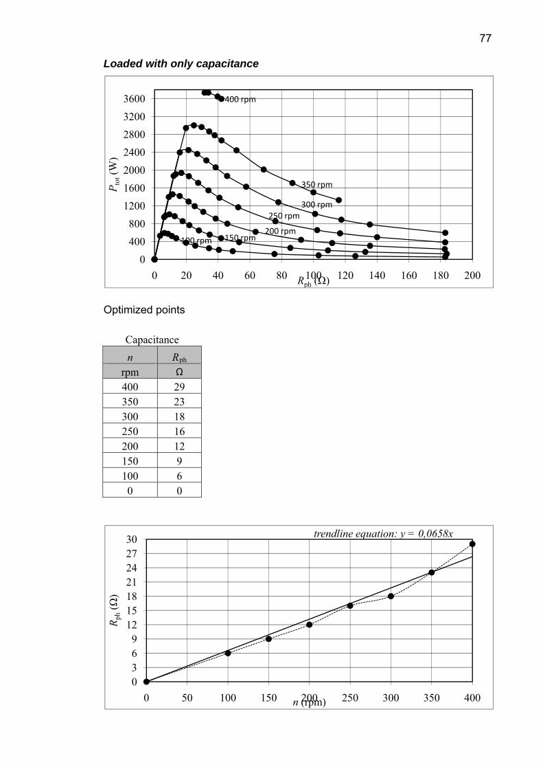
77 Loaded with only capacitance
0400800
1200160020002400280032003600
0 20 40 60 80 100 120 140 160 180 200
P tot
(W)
Rph (Ω)
350 rpm
300 rpm250 rpm
200 rpm150 rpm100 rpm
400 rpm
Optimized points
Capacitance n RRph
rpm Ω 400 29 350 23 300 18 250 16 200 12 150 9 100 6 0 0
trendline equation: y = 0,0658x
0369
12151821242730
0 50 100 150 200 250 300 350 400
R ph
(Ω)
n (rpm)

78 Loaded with capacitance and bridge
0
400
800
1200
1600
2000
2400
2800
3200
0 10 20 30 40 50 60 70 80 90
P tot
(W)
Rph (Ω)
250 rpm
200 rpm
150 rpm
100 rpm
300 rpm
Optimized points
Capacitance + bridge
n RRph rpm Ω 300 21 250 16 200 13 150 9 100 6 0 0
trendline equation: y = 0,066x
02468
1012141618202224
0 50 100 150 200 250 300
R ph
(Ω)
n (rpm)

79 8.1.2 Load seen from DC-side
Note: depends on DC-bridge, these are measurements with our DC-bridge.
Lines with show the power measured before the DC-bridge, lines with show
the power after the DC-bridge. The difference between the two are the losses.
DC-side without capacitance
0200400600800
1000120014001600180020002200
0 20 40 60 80 100 120 140 160
P (W
)
RDC (Ω)
300 rpm
250 rpm200 rpm150 rpm100 rpm
Optimized points
DC - side n RRDC
rpm Ω 300 24 250 21 200 17 150 13 100 9
0 0

80
trendline equation: y = 0,0831x
0369
12151821242730
0 50 100 150 200 250 300
R DC
(Ω)
n (rpm)
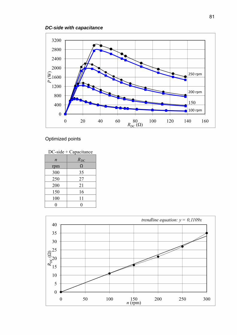
81 DC-side with capacitance
Optimized points
0
400
800
1200
1600
2000
2400
2800
3200
0 20 40 60 80 100 120 140 160
P(W
)
RDC (Ω)
250 rpm
200 rpm
150 100 rpm
DC-side + Capacitance n RRDC
rpm Ω 300 35 250 27 200 21 150 16 100 11 0 0
trendline equation: y = 0,1109x
0
5
10
15
20
25
30
35
40
0 50 100 150 200 250 300
R DC
(Ω)
n (rpm)

82 8.1.3 Conclusion
We can see clearly that the total power is changing depending on speed and
load. We have to notice that the capacitance, which is switched directly after the
generator at the AC side, can boost the total available power to a higher level.
This is due to the neutralization of some generator inductance.
We also notice that the curve with load as a function of the speed is near to lin-
ear. The trend line is shown and the trend line’s equation is calculated. This
equation might be useful when the load has to become adjusted to the genera-
tor speed. A dynamic system using these equations might be a solution.
8.2 First changing speed measurement
This is the first measurement we did with the generator driven by a changing
speed.
0
500
1000
1500
2000
2500
0,000 0,500 1,000 1,500 2,000 2,500 3,000 3,500 4,000 4,500 5,000
Power (W)
Time (s)20 ohm SmallWaves 50 ohm HighWaves20 ohm HighWaves 50 ohm SmallWaves
The horizontal lines represent the average generated power. There are two
waves, the high waves and the small waves. The high waves are higher (ampli-
tude A) and have a longer wavelength.
83
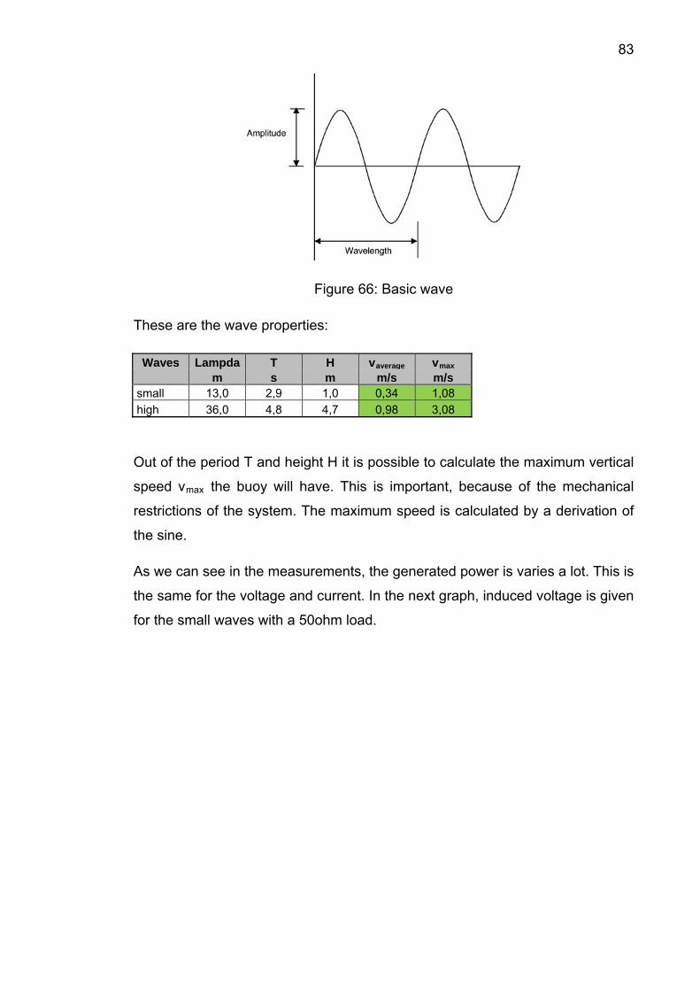
Figure 66: Basic wave
These are the wave properties:
Waves Lampda T H vaverage vmax m s m m/s m/s
small 13,0 2,9 1,0 0,34 1,08 high 36,0 4,8 4,7 0,98 3,08
Out of the period T and height H it is possible to calculate the maximum vertical
speed vmax the buoy will have. This is important, because of the mechanical
restrictions of the system. The maximum speed is calculated by a derivation of
the sine.
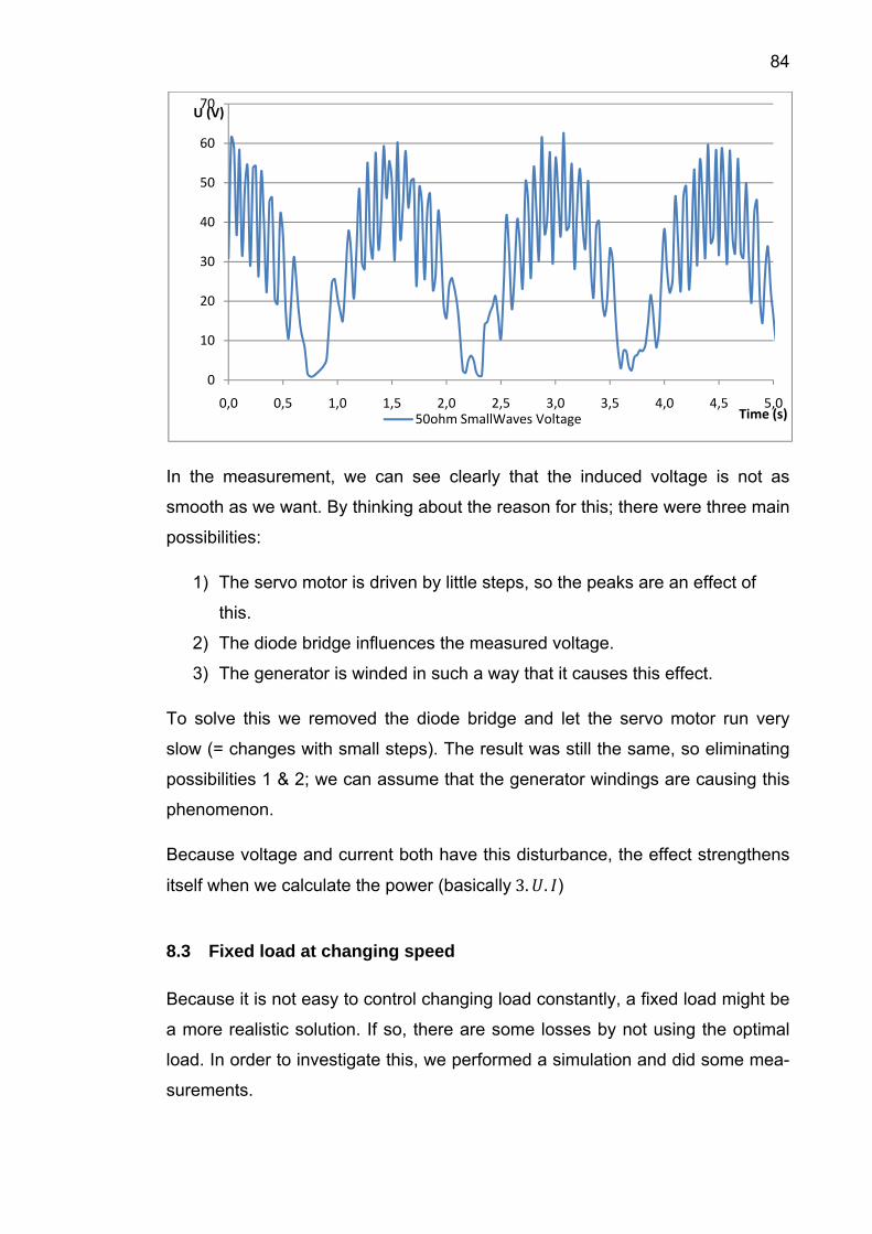
As we can see in the measurements, the generated power is varies a lot. This is
the same for the voltage and current. In the next graph, induced voltage is given
for the small waves with a 50ohm load.
84
0
10
20
30
40
50
60
70
0,0 0,5 1,0 1,5 2,0 2,5 3,0 3,5 4,0 4,5 5,0
U (V)
Time (s)50ohm SmallWaves Voltage
In the measurement, we can see clearly that the induced voltage is not as
smooth as we want. By thinking about the reason for this; there were three main
possibilities:
1) The servo motor is driven by little steps, so the peaks are an effect of
this.
2) The diode bridge influences the measured voltage.
3) The generator is winded in such a way that it causes this effect.
To solve this we removed the diode bridge and let the servo motor run very
slow (= changes with small steps). The result was still the same, so eliminating
possibilities 1 & 2; we can assume that the generator windings are causing this
phenomenon.
Because voltage and current both have this disturbance, the effect strengthens
itself when we calculate the power (basically 3. . )
8.3 Fixed load at changing speed
Because it is not easy to control changing load constantly, a fixed load might be
a more realistic solution. If so, there are some losses by not using the optimal
load. In order to investigate this, we performed a simulation and did some mea-
surements.

85 8.3.1 Fixed load - Model simulation
This is a model simulation for the same high waves as used in 8.2. The model
simulation says that there will be losses, as shown. The red line shows the si-
mulation with an optimized load for each speed. The black line is with a fixed
load.
Red ‐ Rph = 0..14,55 ohm Black ‐ Rph = 14,55 ohm
0
200
400
600
800
1000
1200
1400
1600
1800
2000
0,0 0,5 1,0 1,5 2,0 2,5 3,0 3,5 4,0 4,5 5,0
P tot
(W)
t (s)
Calculation of the average power of both the fixed load and the varying load
gives:
Average power fixed load: , = 1053,46 W
Average power optimized load: , 1209,59 W
We notice a difference of 156,13 W.
8.3.2 Fixed load – Measurements
When we keep the load constant at 14,55Ω the black line shows us the meas-
ured power during a test drive. We can see a small difference between the
theoretical simulated value (red line).

86 When we calculate the average power out of the measurements and the simula-
tion data, this is given:
Average power simulation: , 1046,58 W
Average power measurements: , 1073,19 W
We notice a difference of 26,61 W.
0200400600800
100012001400160018002000
0,0 0,5 1,0 1,5 2,0 2,5 3,0 3,5 4,0 4,5 5,0
P tot
t (s)

87 9 CONCLUSIONS
There are enough possibilities to extract wave energy. The technology is surely
worth further investment.
When working in this field, we have to keep in mind that theoretical models are
not always reliable, and it is difficult to compare them with the reality if there are
no practical examples available. Nevertheless, theoretical models -if dimen-
sioned correctly- are very important to estimate the result. Theoretical modeling
and simulation is a very time consuming activity, but indispensable in this field.
Since the ASWEC project has now a test setting in the lab, the project has
made progress. In the future it will be easier to do practical measurements. The
next step is undoubtedly trying to get energy into the grid.
Nonetheless, further research is required to optimize the boost converter. Now
simulation programs show the usefulness of the boost converter in the project,
further dimensioning and later controlling of the boost converter is necessary.
Measurements on the test setting have showed that the dimensioning of the
load can change the energy extraction. Research on how the load can be con-
stantly optimized may be useful.
While using the servo motor control program, we have to keep in mind that the
computer running the program has to be powerful enough. It is proven that the
measurements of a powerful computer are more precise than the one from a
less powerful computer. The main reason may be that the powerful computer
can take much more measuring points due to a faster processor.
The PSpice simulations of the boost converter have shown that the boost con-
verter is useful. However, other things may be useful to improve the DC voltage
even more. The use of a flywheel might be the first choice. When using this, the
axis is expected to have no stops anymore, which makes sure the generator
keeps on generating (lower) power. The more power there is at the input of the
boost converter, the better it is working. Simulations have shown the boost con-
verter is not able to keep up the output voltage while the input voltage is drop-
ping to zero. The flywheel can help to increase the input voltage when needed.

88 Combined with the flywheel, a capacitance might also be useful. The advantage
with the boost converter might be that the capacitor can be smaller than before.
So, we are still avoiding the use of an expensive super capacitor.
In all the simulations, the boost converter has no control. The next step in the
development of the boost converter might be the design of the control. This
should ensure the boost converter is only working in the points where the vol-
tage is dropping, and the more the voltage drops, the more the converter has to
boost. A good control can help to make the DC-voltage smoother.
Theoretically, the switching frequency of the boost converter can improve the
results. In this thesis only 1 kHz and 10 kHz is simulated. Further research to
find an optimal switching frequency might be useful.
Since the generator is acting very inductive in the simulations (comparable to a
current source), calculations made to calculate the boost converter’s inductance
and the optimized load might be irrelevant in this situation.
89 10 REFERENCES
[1] Book: João Cruz, 2008, Ocean Wave Energy – Current status and future
perspectives, Springer
[2] Book: Godfrey Boyle, 2004, Renewable Energy – Power for a sustainable future, 2nd edition, Oxford
[3] Book: William D’haeseleer, 2005, Energie vandaag en morgen.
Beschouwingen over energievoorziening en -gebruik, ACCO
[4] Book: Mohan/ Undeland/ Robbins, 2003, Power Electronics: Converters,
Applications, and Design, 3rd edition, WILEY
[5] L. Ran, P. Tavner, M. Mueller, N. Baker & S. Mc Donald, “Power Conversion
and Control for a Low Speed, Permanent Magnet, Direct-Drive, Wave Energy
Converter”, Power Electronics Machines and Drives, Dublin 2006.
[6] Paper: Z.Nie, P.C.J. Clifton & R.A. McMahon, 2008, Wave Energy Emulator and AC/DC Rectifiers for Direct Drive Wave Energy Converters, Cambridge University Engineering Department, England
[7] Paper: Gunnar Asplund, Sustainable energy systems with HVDC transmis-
sion
[8] Course: G. Merlevede, Inleiding tot de vermogenselektronica, KHBO