Analysis and Forest Service Visualizationforsys.sefs.uw.edu/Software/FUSION/FUSION_manual.pdf326- W, Whitten Building, 14th and Independence Avenue, SW, Washington, DC 20250-9410 or

United States Department of Agriculture Forest Service Pacific Northwest Research Station

FUSION/LDV: Software for LIDAR Data Analysis and

Visualization

Robert J. McGaughey

August 2018 – FUSION Version 3.80

The Forest Service of the U.S. Department of Agriculture is dedicated to the principle of multiple use management of the Nation’s forest resources for sustained yields of wood, water, forage, wildlife, and recreation. Through forestry research, cooperation with the States and private forest owners, and management of the National Forests and National Grasslands, it strives—as directed by Congress—to provide increasingly greater service to a growing Nation. The U.S. Department of Agriculture (USDA) prohibits discrimination in all its programs and activities on the basis of race, color, national origin, gender, religion, age, disability, political beliefs, sexual orientation, or marital or family status. (Not all prohibited bases apply to all programs.) Persons with disabilities who require alternative means for communication of program information (Braille, large print, audiotape, etc.) should contact USDA’s TARGET Center at (202) 720-2600 (voice and TDD). To file a complaint of discrimination, write USDA, Director, Office of Civil Rights, Room 326- W, Whitten Building, 14th and Independence Avenue, SW, Washington, DC 20250-9410 or call (202) 720-5964 (voice and TDD). USDA is an equal opportunity provider and employer. USDA is committed to making its information materials accessible to all USDA customers and employees.

Author Robert J. McGaughey is a research forester, U.S. Department of Agriculture, Forest Service, Pacific Northwest Research Station, University of Washington, Box 352100, Seattle, WA 98195-2100, [email protected]

Contents FUSION Disclaimer ......................................................................................................... 1 LIDAR Overview .............................................................................................................. 2

How Does LIDAR Work? ............................................................................................. 2 Overview of the FUSION/LDV Analysis and Visualization System .................................. 3 Using FUSION/LDV......................................................................................................... 6

Getting Data into FUSION ........................................................................................... 6 Converting LIDAR Data Files into LDA Files ............................................................... 7

Creating Images Using LIDAR Data ............................................................................ 7 Building a FUSION Project .......................................................................................... 8 FUSION Preferences ................................................................................................... 8

Keyboard Commands for FUSION .................................................................................. 9 Keyboard Commands for LDV ...................................................................................... 10

Keyboard Commands for PDQ ...................................................................................... 14 Command Line Utility and Processing Programs .......................................................... 17

Command Line Options Shared By All Programs ...................................................... 17

Command Log Files ................................................................................................... 17 Reading Compressed LAS Files (LAZ format) ........................................................... 19 FUSION-LTK Overview ............................................................................................. 19

ASCII2DTM ............................................................................................................... 23 ASCIIImport ............................................................................................................... 25

CanopyMaxima .......................................................................................................... 26 CanopyModel ............................................................................................................ 29 Catalog ...................................................................................................................... 34

ClipData ..................................................................................................................... 40 ClipDTM ..................................................................................................................... 44

CloudMetrics .............................................................................................................. 45 Cover ......................................................................................................................... 54

CSV2Grid .................................................................................................................. 57 DensityMetrics ........................................................................................................... 58 DTM2ASCII ............................................................................................................... 61

DTM2ENVI ................................................................................................................ 62 DTM2TIF ................................................................................................................... 63

DTM2XYZ .................................................................................................................. 64 DTMDescribe ............................................................................................................. 65 DTMHeader ............................................................................................................... 66

FilterData ................................................................................................................... 67 FirstLastReturn .......................................................................................................... 70

GridMetrics ................................................................................................................ 72 GridSample ................................................................................................................ 85

GridSurfaceCreate ..................................................................................................... 87 GridSurfaceStats ....................................................................................................... 90 GroundFilter ............................................................................................................... 93 ImageCreate .............................................................................................................. 97 IntensityImage ........................................................................................................... 99 JoinDB ..................................................................................................................... 104

LDA2ASCII .............................................................................................................. 105

LDA2LAS ................................................................................................................. 106 MergeData ............................................................................................................... 108

MergeDTM ............................................................................................................... 110 MergeRaster ............................................................................................................ 113 PDQ ......................................................................................................................... 115 PolyClipData ............................................................................................................ 118 RepairGridDTM........................................................................................................ 121

ReturnDensity .......................................................................................................... 123 SplitDTM .................................................................................................................. 125 SurfaceSample ........................................................................................................ 127 SurfaceStats ............................................................................................................ 131 ThinData .................................................................................................................. 132

TiledImageMap ........................................................................................................ 134 TINSurfaceCreate .................................................................................................... 136

TopoMetrics ............................................................................................................. 138

TreeSeg ................................................................................................................... 141 UpdateIndexChecksum/RefreshIndexChecksum .................................................... 145 ViewPic .................................................................................................................... 147

XYZ2DTM ................................................................................................................ 148 XYZConvert ............................................................................................................. 150

Copyright Notifications ................................................................................................ 152 Acknowledgements ..................................................................................................... 153 References .................................................................................................................. 154

Appendix A: File Formats ............................................................................................ 157 PLANS Surface Models (.DTM) ............................................................................... 158

LIDAR Data Files (.LDA) .......................................................................................... 161 Data Index Files (.LDX and .LDI) ............................................................................. 162

LAS LIDAR Data Files (.LAS) .................................................................................. 164 XYZ Point Files ........................................................................................................ 165 Hotspot Files ............................................................................................................ 166

Tree Files ................................................................................................................. 169 Appendix B: DOS Batch Programming and the FUSION LIDAR Toolkit ..................... 175

Batch Programming Overview ................................................................................. 176 Getting help with batch programming commands .................................................... 176 Using the FUSION Command Line Tools ................................................................ 177

Automating Processing Tasks ................................................................................. 178 Appendix C: Using LTKProcessor to Process Data for Large Acquisitions ................. 180

Overview .................................................................................................................. 181 Considerations for Processing Data from Large Acquisitions .................................. 181

Computer software and hardware conflicts .............................................................. 182 Subdividing large datasets ....................................................................................... 187 Batch File for Pre-processing .................................................................................. 188 Batch File for Processing Individual Data Tiles or Analysis Grid Cells..................... 188 Batch File for Final Processing ................................................................................ 189 Example Batch Files ................................................................................................ 189

Appendix D: Building multi-processor workflows using AreaProcessor ....................... 191

Overview .................................................................................................................. 192 Configuring AreaProcessor on your computer ......................................................... 193

Preparing data for AreaProcessor ........................................................................... 194 Processing tile and block strategies ......................................................................... 195 Processing batch files .............................................................................................. 196 Configuring the run for multiple processors ............................................................. 197 What to do when something goes wrong ................................................................. 198

Appendix E: Retiling point data using AreaProcessor ................................................. 200

Using AreaProcessor to retile point files .................................................................. 201 Appendix F: Using AreaProcessor to produce return density raster layers ................. 205

Appendix G: Converting ESRI GRID data to ASCII raster format using GDAL ........... 208 Overview .................................................................................................................. 209

Converting Data from GRID to ASCII Raster Format ............................................... 209

1

FUSION Disclaimer FUSION and all related programs are developed at the US Department of Agriculture, Forest Service, Pacific Northwest Research Station by an employee of the Federal Government in the course of his official duties. Pursuant to Title 17, Section 105 of the United States Code, this software is not subject to copyright protection and is in the public domain. FUSION is primarily a research tool. USDA Forest Service assumes no responsibility whatsoever for its use by other parties, and makes no guarantees, expressed or implied, about its quality, reliability, or any other characteristic.

2

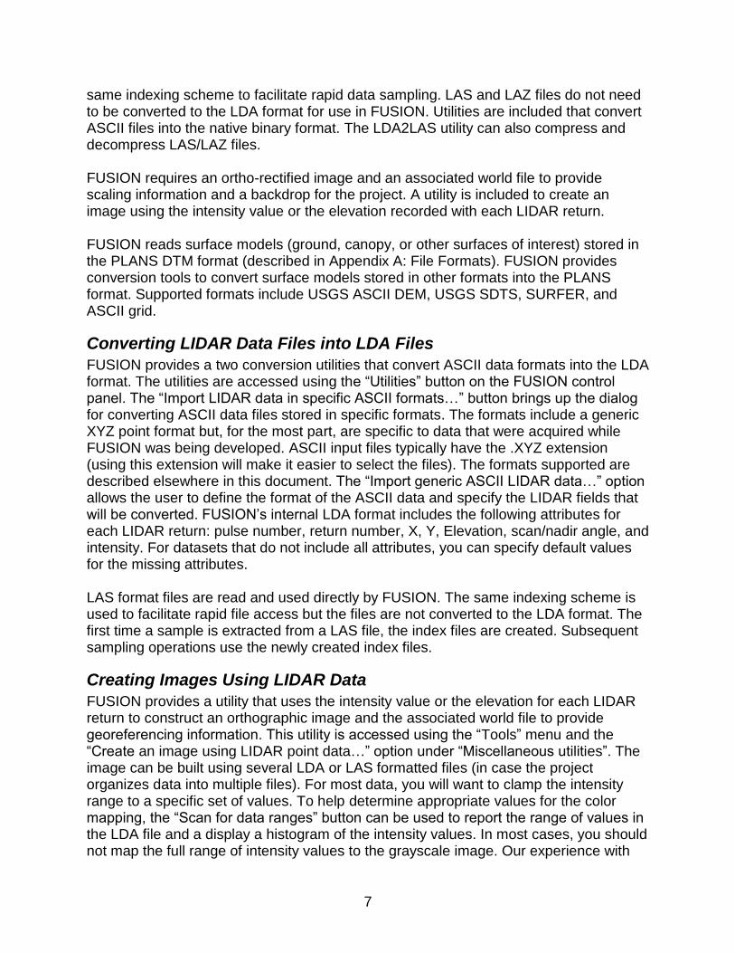
LIDAR Overview Light detection and ranging systems (LIDAR) use laser light to measure distances. They are used in many ways, from estimating atmospheric aerosols by shooting a laser skyward to catching speeders in freeway traffic with a handheld laser-speed detector. Airborne laser-scanning technology is a specialized, aircraft-based type of LIDAR that provides extremely accurate, detailed 3-D measurements of the ground, vegetation, and buildings. Developed in just the last 15 years, one of LIDAR’s first commercial uses in the United States was to survey power line corridors to identify encroaching vegetation. Additional uses include mapping landforms and coastal areas. In open, flat areas, ground contours can be recorded from an aircraft flying overhead providing accuracy within 6 inches of actual elevation. In steep, forested areas accuracy is typically in the range of 1 to 2 feet and depends on many factors, including density of canopy cover and the spacing of laser shots. The speed and accuracy of LIDAR made it feasible to map large areas with the kind of detail that before had only been possible with time-consuming and expensive ground survey crews.

Figure 1. Schematic of an airborne laser scanning system.

Federal agencies such as the Federal Emergency Management Administration (FEMA) and U.S. Geological Survey (USGS), along with county and state agencies, began using LIDAR to map the terrain in flood plains and earthquake hazard zones. The Puget Sound LIDAR Consortium, an informal group of agencies, used LIDAR in the Puget Sound area and found previously undetected earthquake faults and large, deep-seated, old landslides. In other parts of the country, LIDAR was used to map highly detailed contours across large flood plains, which could be used to pinpoint areas of high risk. In some areas, entire states have been flown with LIDAR to produce more accurate digital terrain data for emergency planning and response. LIDAR mapping of terrain uses a technique called “bare-earth filtering.” Laser scan data about trees and buildings are stripped away, leaving just the bare-ground data. Fortunately for foresters and other natural resource specialists, the data being “thrown away” by geologists provide detailed information describing vegetation conditions and structure.

How Does LIDAR Work?

The use of lasers has become commonplace, from laser printers to laser surgery. In airborne-laser-mapping, LIDAR systems are taken into the sky. Instruments are

3

mounted on a single- or twin-engine plane or a helicopter and data are collected over large land areas. Airborne LIDAR technology uses four major pieces of equipment (Figure 1). These are a laser emitter-receiver scanning unit attached to the aircraft; global positioning system (GPS) units on the aircraft and on the ground; an inertial measurement unit (IMU) attached to the scanner, which measures roll, pitch, and yaw of the aircraft; and a computer to control the system and store data. Several types of airborne LIDAR systems have been developed; commercial systems commonly used in forestry are discrete-return, small-footprint systems. “Small footprint” means that the laser beam diameter at ground level is typically in the range of 6 inches to 3 feet. The laser scanner on the aircraft sends up to 200,000 pulses of light per second to the ground and measures how long it takes each pulse to reflect back to the unit. These times are used to compute the distance each pulse traveled from scanner to ground. The GPS and IMU units determine the precise location and attitude of the laser scanner as the pulses are emitted, and an exact coordinate is calculated for each point. The laser scanner uses an oscillating mirror or rotating prism (depending on the sensor model), so that the light pulses sweep across a swath of landscape below the aircraft. Large areas are surveyed with a series of parallel flight lines. The laser pulses used are safe for people and all living things. Because the system emits its own light, flights can be done day or night, as long as the skies are clear. Thus, with distance and location information accurately determined, the laser pulses yield direct, 3-D measurements of the ground surface, vegetation, roads, and buildings. Millions of data points are recorded; so many that LIDAR creates a 3-D data cloud. After the flight, software calculates the final data points by using the location information and laser data. Final results are typically produced in weeks, whereas traditional ground-based mapping methods took months or years. The first acre of a LIDAR flight is expensive, owing to the costs of the aircraft, equipment, and personnel. But when large areas are covered, the costs can drop to about $1 to $2 per acre. The technology is commercially available through a number of sources.

Overview of the FUSION/LDV Analysis and Visualization System The FUSION/LDV software was originally developed to help researchers understand, explore, and analyze LIDAR data. The large data sets commonly produced by LIDAR missions could not be used in commercial GIS or image processing environments without extensive preprocessing. Simple tasks such as extracting a sample of LIDAR returns that corresponded to a field plot were complicated by the sheer size of the data and the variety of ASCII text formats provided by various vendors. The original versions of the software allowed users to clip data samples and view them interactively. As a new data set was delivered, the software was modified to read the data format and features were added depending on the needs of a particular research project. After a year or so of activity, scientists at the Pacific Northwest Research Station and the University of Washington decided to design a more comprehensive system to support their research efforts.

4

The analysis and visualization system consists of two main programs, FUSION and LDV (LIDAR data viewer), and a collection of task-specific command line programs. The primary interface, provided by FUSION, consists of a graphical display window and a control window. The FUSION display presents all project data using a 2D display typical of geographic information systems. It supports a variety of data types and formats including shapefiles, images, digital terrain models, canopy surface models, and LIDAR return data. LDV provides the 3D visualization environment for the examination and measurement of spatially-explicit data subsets. Command line programs provide specific analysis and data processing capabilities designed to make FUSION suitable for processing large LIDAR acquisitions. In FUSION, data layers are classified into six categories: images, raw data, points of interest, hotspots, trees, and surface models. Images can be any geo-referenced image but they are typically orthophotos, images developed using intensity or elevation values from LIDAR return data, or other images that depict spatially explicit analysis results. Raw data include LIDAR return data and simple XYZ point files. Points of interest (POI) can be any point, line, or polygon layer that provides useful visual information or sample point locations. Hotspots are spatially explicit markers linked to external references such as images, web sites, or pre-sampled data subsets. Tree files contain data, usually measured in the field, representing individual trees. Surface models, representing the bare ground or canopy surface, must be in a gridded format. FUSION uses the PLANS format for its surface models and provides utilities to convert a variety of formats into the PLANS format. The current FUSION implementation limits the user to a single image, surface model, and canopy model, however, multiple raw data, POI, tree, and hotspot layers are allowed. The FUSION interface provides users with an easily understood display of all project data. Users can specify display attributes for all data and can toggle the display of the different data types. FUSION allows users to quickly and easily select and display subsets of large LIDAR data. Users specify the subset size, shape, and the rules used to assign colors to individual raw data points and then select sample locations in the graphical display or by manually entering coordinates for the points defining the sample. LDV presents the subset for the user to examine. Subsets include not only raw data but also the portion of the image and surface models for the area sampled. FUSION provides the following data subset types:

Fixed-size square,

Fixed-size circle,

Variable-size square,

Variable-size circle,

Variable-width corridor. Subset locations can be “snapped” to a specific sample location, defined by POI points to generate subsets centered on or defined by specific locations. Elevation values for LIDAR returns can be normalized using the ground surface model prior to display in LDV. This feature is especially useful when viewing data representing forested regions

5

in steep terrain as it is much easier to examine returns from vegetation and compare trees after subtracting the ground elevation. LDV strives to make effective use of color, lighting, glyph shape, motion, and stereoscopic rendering to help users understand and evaluate LIDAR data. Color is used to convey one or more attributes of the LIDAR data or attributes derived from other data layers. For example, individual returns can be colored using values sampled from an orthophoto of the project area to produce semi-photorealistic visual simulations. LDV uses a variety of shading and lighting methods to enhance its renderings. LDV provides point glyphs that range from single pixels, to simple geometric objects, to complex superquadric objects. LDV operates in monoscopic, stereoscopic, and anaglyph display modes. To enhance the 3D effect on monoscopic display systems, LDV provides a simple rotation feature that moves the data subset continuously through a simple pattern (usually circular). We have dubbed this technique “wiggle vision”, and feel it provides a much better sense of the 3D spatial arrangement of points than provided by a static, fixed display. To further help users understand LIDAR data, LDV can also map orthographic images onto a horizontal plane that can be positioned vertically within the cloud of raw data points. Bare-earth surface models are rendered as a shaded 3D surface and can be textured-mapped using the sampled image. Canopy surface or canopy height models are rendered as a mesh so the viewer can see the data points under the surface. FUSION and LDV have several features that facilitate direct measurement of LIDAR data. FUSION provides a “plot mode” that defines a buffer around the sample area and includes data from the buffer in a data subset. This option, available only with fixed-size plots, makes it easy to create LIDAR data subsets that correspond to field plots. “Plot mode” lets the user measure tree attributes for trees whose stem is within the plot area using all returns for the tree including those outside the plot area but within the plot buffer. The size of the plot buffer is usually set to include the crown of the largest trees expected for a site. When in “plot mode”, FUSION includes a description of the fixed-area portion of the subset so LDV can display the plot boundary as a wire frame cylinder or cube and inform the user when measurement locations are within or outside the plot boundary.. LDV provides several functions to help users place the measurement marker and make measurements within the data cloud. The following “snap functions” are available to help position the measurement marker:

Set marker to the elevation of the lowest point in the current measurement area (don’t move XY position of marker)

Set marker to the elevation of the highest point in the current measurement area (don’t move XY position of marker)

Set marker to the elevation of the point closest to the marker (don’t move XY position of marker)

Move marker to the lowest point in the current measurement area

Move marker to the highest point in the current measurement area

Move marker to point closest to the marker

6

Set marker to the elevation of the surface model (usually the ground surface)

Change the shape and alignment of the measurement marker to better fit the data points that represent a tree crown

The measurement marker in LDV can be elliptical or circular to compensate for tree crowns that are not perfectly round. The measurement area can be rotated to better align with an individual tree crown. Once an individual tree has been isolated and measured, the points within the measurement area can be “turned off” to indicate that they have been considered during the measurement process. This ability makes it much easier to isolate individual trees in stands with dense canopies.

Using FUSION/LDV To start using the FUSION system, launch FUSION and load the example project named “demo_4800K.dvz” using the File…Open menu option. The default sample options are set to use a stroked box. LIDAR returns will be colored according to their height above ground. To extract and display a sample of data, stroke a rectanglar area using the mouse. The status display in the lower left corner of the FUSION window shows the size of the stroked area. Try for a sample that is about 250 feet by 250 feet. This should yield a sample of about 22,000 points. After a short time, the data subset will be displayed in LDV. To facilitate rapid sample extraction, FUSION uses a simple indexing scheme to organize the LIDAR data. This indexing process is necessary the first time FUSION uses a new dataset. Subsequent samples will take less time because the data files only need to be indexed once. To manipulate the LIDAR data in LDV, it is easiest to imagine that the data is contained in a glass ball. To rotate the data, use the mouse (with the left button held down) to roll the ball and thus manipulate the data. As you move the data, LDV may display only a subset of the points depending on the size of the sample. Options in LDV are accessed using the right mouse button to activate a menu of options. There are many options and the best way to understand them is to try them. Additional functions are assigned to keystrokes. These functions are described when you click the “About LDV” button located in the lower left corner of the LDV window. Keyboard shortcuts are also listed on the right mouse menu.

Getting Data into FUSION

FUSION merges imagery, LIDAR data, GIS layers, field data, and surface models to provide an intuitive interface to large project datasets. FUSION requires an ortho-rectified image for the project area (image can be created in FUSION using LIDAR return data) and LIDAR data. Other data types are optional. FUSION currently reads several ASCII file formats, LAS files, and compressed LAS files (LAZ format). Its native format, called LDA, is an indexed binary format that allows rapid random access to large datasets. FUSION also reads LAS and LAZ files and uses the

7

same indexing scheme to facilitate rapid data sampling. LAS and LAZ files do not need to be converted to the LDA format for use in FUSION. Utilities are included that convert ASCII files into the native binary format. The LDA2LAS utility can also compress and decompress LAS/LAZ files. FUSION requires an ortho-rectified image and an associated world file to provide scaling information and a backdrop for the project. A utility is included to create an image using the intensity value or the elevation recorded with each LIDAR return. FUSION reads surface models (ground, canopy, or other surfaces of interest) stored in the PLANS DTM format (described in Appendix A: File Formats). FUSION provides conversion tools to convert surface models stored in other formats into the PLANS format. Supported formats include USGS ASCII DEM, USGS SDTS, SURFER, and ASCII grid.

Converting LIDAR Data Files into LDA Files

FUSION provides a two conversion utilities that convert ASCII data formats into the LDA format. The utilities are accessed using the “Utilities” button on the FUSION control panel. The “Import LIDAR data in specific ASCII formats…” button brings up the dialog for converting ASCII data files stored in specific formats. The formats include a generic XYZ point format but, for the most part, are specific to data that were acquired while FUSION was being developed. ASCII input files typically have the .XYZ extension (using this extension will make it easier to select the files). The formats supported are described elsewhere in this document. The “Import generic ASCII LIDAR data…” option allows the user to define the format of the ASCII data and specify the LIDAR fields that will be converted. FUSION’s internal LDA format includes the following attributes for each LIDAR return: pulse number, return number, X, Y, Elevation, scan/nadir angle, and intensity. For datasets that do not include all attributes, you can specify default values for the missing attributes. LAS format files are read and used directly by FUSION. The same indexing scheme is used to facilitate rapid file access but the files are not converted to the LDA format. The first time a sample is extracted from a LAS file, the index files are created. Subsequent sampling operations use the newly created index files.

Creating Images Using LIDAR Data

FUSION provides a utility that uses the intensity value or the elevation for each LIDAR return to construct an orthographic image and the associated world file to provide georeferencing information. This utility is accessed using the “Tools” menu and the “Create an image using LIDAR point data…” option under “Miscellaneous utilities”. The image can be built using several LDA or LAS formatted files (in case the project organizes data into multiple files). For most data, you will want to clamp the intensity range to a specific set of values. To help determine appropriate values for the color mapping, the “Scan for data ranges” button can be used to report the range of values in the LDA file and a display a histogram of the intensity values. In most cases, you should not map the full range of intensity values to the grayscale image. Our experience with

8

several vendors has taught us that most vendors don’t know much about the intensity values and can’t even tell you the correct range of values recorded in their data. You can change the pixel size for the image but the default of 1 unit (same planimetric units in LIDAR data) generally provides a reasonable image. For low density datasets (<1 return per square meter), increasing the pixel size will produce an image with fewer voids and will decrease the size of the image file. FUSION provides command line programs that also produce intensity images from LIDAR data. The first, ImageCreate, basically duplicates the functions described above. The second program, IntensityImage, was developed more recently to produce more useful images using the LIDAR intensity data. IntensityImage provides automatic scaling for the range of intensity values and incorporates a point to pixel conversion process that helps create high-resolution images from LIDAR point data.

Building a FUSION Project

Once you have an image and some LIDAR data files, you are ready to build the FUSION project. Click the “Image…” button and select the image you created from the LIDAR data values. Next, click the “Raw data…” button and select LAS files or the LDA files created from your ASCII data files. The default symbol type, “None”, is suitable for most projects so just click the OK button. When the symbol type is set to “None”, FUSION will draw a box that represents the extent of each indexed LIDAR data file when you “turn-on” display of the raw data. You now have a FUSION project ready to go. Click the “Sample options” button to specify sampling options for the LIDAR subsets, or just stroke a rectangular area to cut out a subset of data and launch the 3D viewer. The first time data files are used with FUSION, they will be indexed. The indexing process may take a few minutes depending on the size of the project area and LIDAR return density. Indexing is only done once so subsequent samples will display much faster.

FUSION Preferences

FUSION provides a number of setting to control its overall behavior. These include communications settings for using a GPS receiver to provide a “moving marker” showing the current GPS in the FUSION display, settings for the buffer used when FUSION is in “plot mode”, and setting that control how FUSION clips data for display in LDV and the location used to store temporary files. For many managed computer systems, users do not have access to all folders. In many configurations, users may not have permission to write files into the “Program Files” folder or other folders where FUSION might be installed. When FUSION is used in such environments, the option to store temporary data files in the user’s temporary folder should be checked to ensure that FUSION can pass data sample to LDV. If this option is not enabled, you will often get a message indicating that there are no data points within the sample area even when you know for sure that you are sampling within the data coverage area.

9

Keyboard Commands for FUSION The following keystroke and mouse commands area available in FUSION after an image has been loaded.

Keystroke/mouse action

Description

Middle mouse button

Pan the display to the location of the mouse cursor

Left mouse button Begin a sample using the location of the mouse cursor

Right mouse button

Cancel a sample (the right mouse button must be pressed while the left button is pressed)

Mouse wheel up/down

Scroll the display up and down

Shift & mouse wheel up/down

Scroll the display left and right

Ctrl & mouse wheel up/down

Zoom the display in and out

Left arrow Pan display to the right

Right arrow Pan display to the left

Up arrow Pan display down

Down arrow Pan display up

(+) plus key Zoom in

(-) minus key Zoom out

Home Zoom to image extent

F5 Redraw the display

10

Keyboard Commands for LDV The following keystroke and mouse commands are available in LDV. Many of these commands can also be accessed using the right-mouse menu.


Context Description

Up arrow 8 on numeric keypad

Viewing Rotate around screen X axis (away from viewer)

Down arrow 2 on numeric keypad

Viewing Rotate around screen X axis (toward viewer)

Right arrow 6 on numeric keypad

Viewing Rotate around screen Y axis (away from viewer)

Left arrow 4 on numeric keypad

Viewing Rotate around screen Y axis (toward viewer)

Page up 9 on numeric keypad

Viewing Rotate around screen Z axis (counter-clockwise)

Page down 3 on numeric keypad

Viewing Rotate around screen Z axis (clockwise)

Home 5 on numeric keypad 7 on numeric keypad

Viewing Reset rotation to original state

Shift & right mouse drag

Measurement marker on

Raise/lower the measurement marker

Mouse wheel Measurement marker on

Raise/lower the measurement marker

Ctrl & right mouse drag


Move measurement marker

Ctrl & Shift & right mouse drag


Increase/decrease measurement marker diameter

Shift & left arrow Measurement marker on

Move marker in negative direction along the X axis of the data (not X axis of screen)

Control & left arrow


Rotate marker 1 degree in positive direction

Shift & control & left arrow


Rotate marker 10 degrees in positive direction

Shift & right arrow Measurement marker on

Move marker in positive direction along the X axis of the data (not X axis of screen)

11


Context Description

Control & right arrow


Rotate marker 1 degree in negative direction

Shift & control & right arrow


Rotate marker 10 degrees in negative direction

Shift & up arrow Measurement marker on

Move marker in positive direction along the Y axis of the data (not Y axis of screen)

Control & up arrow Measurement marker on

Increase long axis of marker making the marker more elliptical (small step)

Shift & control & up arrow


Increase long axis of marker making the marker more elliptical (large step)

Shift & down arrow Measurement marker on

Move marker in negative direction along the Y axis of the data (not Y axis of screen)

Control & down arrow


Decrease long axis of marker making the marker more elliptical (small step)

Shift & control & down arrow


Decrease long axis of marker making the marker more elliptical (large step)

Escape Wiggle-vision on Scan-vision on Measurement marker on

Stop motion or stop scanning of clipping planes Clear marks and measurement points

Backspace Measurement marker on with measurement line

Deletes last measurement point

Enter Measurement marker on

Save measurement point

Space Viewing Activate right-mouse-button menu

+ (plus key) Viewing with image plate active

Increase transparency of the image plate

+ (plus key) Viewing with surface active

Increase transparency of the surface model

Control & + (plus key)

Viewing using fixed size markers

Increase size of point markers

- (minus key) Viewing with image plate active

Decrease transparency of the image plate

- (minus key) Viewing with surface active

Decrease transparency of the surface model

Control & - (minus key)

Viewing using fixed size markers

Decrease size of point markers

12


Context Description

Letter A Measurement marker on

Turn on display of points within measurement area and above current marker height

Shift & letter A Viewing Turn on display of all data points

Letter B Measurement marker on

Turn on display of points within measurement area and below current marker height

Letter C Measurement marker on

Move marker to the height of the closest point within the measurement area

Shift & letter C Measurement marker on

Center the measurement area on the closest point and move the marker to the height of the closest point within the measurement area

Letter F Measurement marker on

Fits the measurement marker to the data points above the measurement plate. Use this option to rotate and adjust the dimensions of the marker to better “fit” the marker to a tree crown.

Letter G Measurement marker on and surface display enabled

Move measurement marker to ground elevation

Letter H Measurement marker on

Move marker to the height of the highest point within the measurement area

Shift & letter H Measurement marker on

Center the measurement area on the highest point and move the marker to the height of the highest point within the measurement area

Letter I Image plate enabled

Lower image plate (small step)

Shift & letter I Image plate enabled

Raise image plate (small step)

Control & letter I Image plate enabled

Lower image plate (large step)

Shift & letter I Image plate enabled

Raise image plate (large step)

Letter L Measurement marker on

Move marker to the height of the lowest point within the measurement area

Shift & letter L Measurement marker on

Center the measurement area on the lowest point and move the marker to the height of the lowest point within the measurement area

Letter O Measurement marker on

Reset measurement marker to a circle

13


Context Description

Letter R Measurement marker on

Turn off display of points within measurement area

Letter S Measurement marker on

Move measurement area to the current marked point (indicated with a 3D “+”)

Letter T Measurement marker on

Toggle display of points within measurement area

Letter X YZ clipping enabled

Lower clipping plane (small step)

Shift & letter X YZ clipping enabled

Raise clipping plane (small step)

Control & letter X YZ clipping enabled

Lower clipping plane (large step)

Shift & letter X YZ clipping enabled

Raise clipping plane (large step)

Letter Y XZ clipping enabled


Shift & letter Y XZ clipping enabled


Control & letter Y XZ clipping enabled


Shift & letter Y XZ clipping enabled


Letter Z XY clipping enabled


Shift & letter Z XY clipping enabled


Control & letter Z XY clipping enabled


Shift & letter Z XY clipping enabled


F3 Viewing Open ground augmentation point dialog

F4 Viewing Open bare ground model dialog*

F5 Viewing Open segmentation dialog*

F7 Viewing Open plot location dialog*

F8 Viewing Open attribute clipping dialog

F9 Viewing Open tree measurement dialog

*These features are considered experimental and not available in publicly released versions of FUSION/LDV.

14

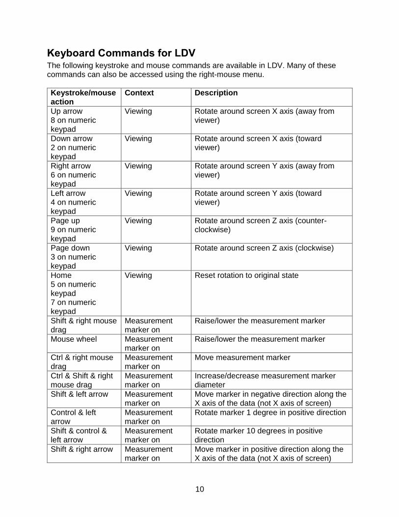
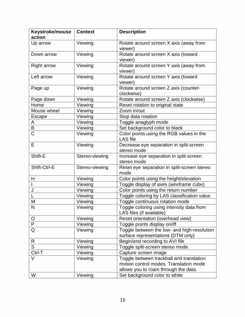
Keyboard Commands for PDQ PDQ is a data visualization tool that provides a more robust data structure and provides more responsive manipulation of large point clouds. It can be used in place of LDV to view samples generated by FUSION by checking the box next to “Use PDQ” in the FUSION control panel. PDQ does not offer the same capabilities as LDV so it may not be suitable for all applications. The following keystroke and mouse commands are available in PDQ. PDQ offers a few special capabilities to help evaluate and view data:

Shade data using the intensity value for each return. Low intensity values are colored brown and high Values are colored green.

Shade data points using the LAS classification codes (LAS format files only). Color returns according to the value in the LAS classification field. The colors are shown in Figure 2.

Color returns using the RGB value stored in the point records within LAS files. By default, PDQ will use the RGB values, when present, to color points in LAS format files.

Provide a scanning mode useful when viewing .DTM format files representing ground and canopy surfaces. This mode sets up an overhead view and allows you to move the surface under the point-of-view using the “+” and “-“ keys.

PDQ supports drag-and-drop for .LDA, .LAS, and .DTM files so you can view files by simply dragging them from a folder view and dropping them into PDQ’s window.

Figure 2. Colors used to represent LAS classification codes in PDQ.

0 Created, never classified 1 Unclassified 2 Ground 3 Low vegetation 4 Medium vegetation 5 High vegetation 6 Building 7 Low point (noise) 8 Model key-point (mass point) 9 Water 10 Reserved 11 Reserved 12 Overlap points 13+ Reserved

15


Context Description

Up arrow Viewing Rotate around screen X axis (away from viewer)

Down arrow Viewing Rotate around screen X axis (toward viewer)

Right arrow Viewing Rotate around screen Y axis (away from viewer)

Left arrow Viewing Rotate around screen Y axis (toward viewer)

Page up Viewing Rotate around screen Z axis (counter-clockwise)

Page down Viewing Rotate around screen Z axis (clockwise)

Home Viewing Reset rotation to original state

Mouse wheel Viewing Zoom in/out

Escape Viewing Stop data rotation

A Viewing Toggle anaglyph mode

B Viewing Set background color to black

C Viewing Color points using the RGB values in the LAS file

E Viewing Decrease eye separation in split-screen stereo mode

Shift-E Stereo-viewing Increase eye separation in split-screen stereo mode

Shift-Ctrl-E Stereo-viewing Reset eye separation in split-screen stereo mode

H Viewing Color points using the height/elevation

I Viewing Toggle display of axes (wireframe cube)

J Viewing Color points using the return number

L Viewing Toggle coloring by LAS classification value

M Viewing Toggle continuous rotation mode

N Viewing Toggle coloring using intensity data from LAS files (if available)

O Viewing Reset orientation (overhead view)

P Viewing Toggle points display on/iff

Q Viewing Toggle between the low- and high-resolution surface representations (DTM only)

R Viewing Begin/end recording to AVI file

S Viewing Toggle split-screen stereo mode

Ctrl-T Viewing Capture screen image

V Viewing Toggle between trackball and translation motion control modes. Translation mode allows you to roam through the data.

W Viewing Set background color to white

16


Context Description

X Stereo-viewing Toggle x-eyed/parallel-eyed viewing in split-screen mode

Z DTM-scanning Lower DTM while in scanning mode

Shift-Z DTM-scanning Raise DTM while in scanning mode

Ctrl + Viewing Increase symbol size

Ctrl - Viewing Decrease symbol size

F5 Viewing Toggle scanning mode for DTM evaluation use + and - to move model

17

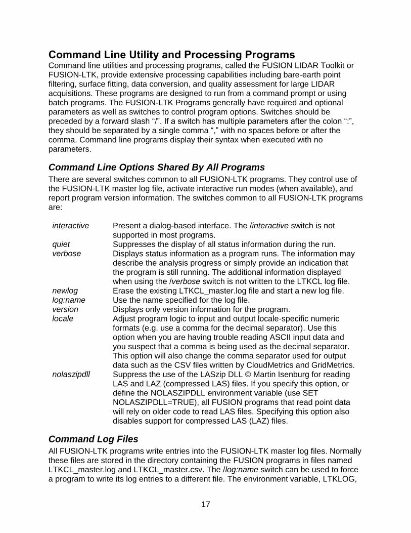
Command Line Utility and Processing Programs Command line utilities and processing programs, called the FUSION LIDAR Toolkit or FUSION-LTK, provide extensive processing capabilities including bare-earth point filtering, surface fitting, data conversion, and quality assessment for large LIDAR acquisitions. These programs are designed to run from a command prompt or using batch programs. The FUSION-LTK Programs generally have required and optional parameters as well as switches to control program options. Switches should be preceded by a forward slash “/”. If a switch has multiple parameters after the colon “:”, they should be separated by a single comma “,” with no spaces before or after the comma. Command line programs display their syntax when executed with no parameters.

Command Line Options Shared By All Programs

There are several switches common to all FUSION-LTK programs. They control use of the FUSION-LTK master log file, activate interactive run modes (when available), and report program version information. The switches common to all FUSION-LTK programs are: interactive Present a dialog-based interface. The /interactive switch is not

supported in most programs. quiet Suppresses the display of all status information during the run. verbose Displays status information as a program runs. The information may

describe the analysis progress or simply provide an indication that the program is still running. The additional information displayed when using the /verbose switch is not written to the LTKCL log file.

newlog Erase the existing LTKCL_master.log file and start a new log file. log:name Use the name specified for the log file. version Displays only version information for the program. locale Adjust program logic to input and output locale-specific numeric

formats (e.g. use a comma for the decimal separator). Use this option when you are having trouble reading ASCII input data and you suspect that a comma is being used as the decimal separator. This option will also change the comma separator used for output data such as the CSV files written by CloudMetrics and GridMetrics.

nolaszipdll Suppress the use of the LASzip DLL © Martin Isenburg for reading LAS and LAZ (compressed LAS) files. If you specify this option, or define the NOLASZIPDLL environment variable (use SET NOLASZIPDLL=TRUE), all FUSION programs that read point data will rely on older code to read LAS files. Specifying this option also disables support for compressed LAS (LAZ) files.

Command Log Files

All FUSION-LTK programs write entries into the FUSION-LTK master log files. Normally these files are stored in the directory containing the FUSION programs in files named LTKCL_master.log and LTKCL_master.csv. The /log:name switch can be used to force a program to write its log entries to a different file. The environment variable, LTKLOG,

18

can also be used to change the default log file. When using LTKLOG, set the variable to the full path for the log file (include the folder) unless you want the log file created in the current directory. The .csv log name will be created from the LTKLOG variable using and extension of .csv. The LTKLOG environment variable can be set from a command prompt using the following DOS command:

set LTKLOG=mylogfile.log

Once the variable is set, it will be available for all programs run in the same DOS window (command prompt window). Other windows will not be able to “see” the variable. The variable can be cleared using the following DOS command:

set LTKLOG=

Use of the LTKLOG environment variable is most effective when the variable is set at the beginning of a batch program used to accomplish some processing task and cleared at the end of the program. In this way you can direct all log entries associated with a project to the same log files. The .log entries include all output normally displayed on the screen when one of the FUSION-LTK programs runs. All command line parameters are reported and any output files are listed along with their creation date and time. Output related to the use of the /verbose switch is not included in the log file. The .csv entries simply list the command lines used to invoke various FUSION-LTK programs. The following columns are included in the .csv log:

Program name Version Program build date Command line parameters Start time Stop time Elapsed time (seconds) Status indicator

The logs have proven very useful when trying to remember the command line options used to create a specific output product or the program version used to conduct an analysis. By matching the file name, date and time to a log entry, you can easily repeat a processing task. The log file can become quite large over time so it is important to either manage the log by archiving the file and then deleting it (a new log file will be started the next time FUSION-LTK program is used) or by using specific log files for different projects. The latter option is facilitated by the /log:name switch but this switch must be used for all programs that are to write to the specified log file. Using the LTKLOG (see Appendix B: DOS Batch Programming and the FUSION LIDAR Toolkit for details) environment variable allows you to change the log file without specifying the log on each program command line.

19

Reading Compressed LAS Files (LAZ format)

All command line programs, FUSION, and PDQ can read compressed LAS files stored in the LAZ format developed by Martin Isenburg if the LASzip DLL is installed in the FUSION install folder. The DLL is available on the LAStools website (the DLL is distributed as part of LAStools). To install the DLL, unpack the LAStools distribution and copy the laszip.dll file from the lastools\LASzip\dll folder to the folder where FUSION is installed. When the DLL is available, FUSION programs will use it to read LAS and LAZ format files. You can disable use of the DLL using either the NOLASZIPDLL environment variable or the /nolaszipdll option available for all command line programs. To disable use of the DLL using the environment variable, use the following command in a command prompt window prior to running FUSION programs: set NOLASZIPDLL=TRUE

To enable use of the DLL in the same command prompt window, clear the variable as follows: set NOLASZIPDLL=

Compressed LAS files (LAZ format) are typically 75-85% smaller than the corresponding LAS format file. However, using LAZ files will be slower than similar operations using LAS files. The FUSION viewing system does not perform well when using compressed files. Extracting and viewing even small samples takes much longer compared to the times when using uncompressed data. Command line tools all perform well with compressed data. The FUSION utility LDA2LAS can be used to compress and decompress LAS files. Input for LDA2LAS is not limited to FUSION’s older LDA format.

FUSION-LTK Overview

The command line utility and processing programs are grouped into six types: Point Operates on point data. Surface Operates on surfaces. Image Operates on images. Conversion Converts data from one format to another. Info Provides descriptive information for a data source. Misc Miscellaneous utilities.

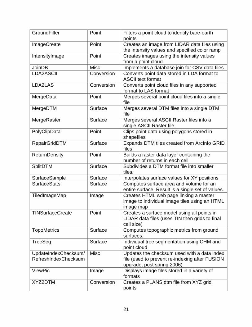
In general, Point utilities use point cloud data to produce either new point clouds or surfaces and Surface utilities use surfaces to produce new surfaces or point data. The set of programs included in the toolkit has, and will continue to, evolve as new analysis methods are discovered or developed. The current set of programs addresses most tasks commonly needed when LIDAR data are obtained for a forestry-related project. The following table summarizes the toolkit programs:

20

Program name Category Description

ASCII2DTM Conversion Converts an ASCII raster surface model into the PLANS format used by FUSION

ASCIIImport Conversion Converts variable format ASCII LIDAR data to LDA or LAS format

CanopyModel Point Creates a canopy surface model from a point cloud

Catalog Point Prepares a report describing a LIDAR dataset and optionally indexes all data files for use in FUSION

ClipData Point Clips subsamples of data using the lower left and upper right corners of the area

ClipDTM Surface Clips a portion of a DTM using a user-specified extent.

CloudMetrics Point Computes metrics for a LIDAR data set (usually a data sample)

Cover Point Computes cover estimates using a bare-earth surface model and point cloud

CSV2Grid Conversion Converts data stored in commas separated value (CSV) format into PLANS dtm format

DensityMetrics Point Computes point density metrics using elevation-based slices

DTM2ASCII Conversion Converts PLANS dtm files into ASCII raster format

DTM2ENVI Conversion Converts PLANS dtm files into ENVI standard format files with associated header files

DTM2TIF Conversion Converts PLANS dtm files into TIF grayscale images

DTM2XYZ Conversion Converts PLANS dtm files into XYZ points

DTMDescribe Misc Outputs information from PLANS dtm file headers to CSV file

DTMHeader Info Display header information for PLANS format surface models and edit some header elements

FilterData Point Applies various filters to return data

FirstLastReturn Point Extracts first and last returns from a point cloud

GridMetrics Point Computes metrics for points falling within each grid cell

GridSample Surface Extracts samples of grid values around an XY position

GridSurfaceCreate Point Creates a gridded surface model from point data

GridSurfaceStats Surface Computes surface area and volume for the surface. Result is a raster layer.

21

GroundFilter Point Filters a point cloud to identify bare-earth points

ImageCreate Point Creates an image from LIDAR data files using the intensity values and specified color ramp

IntensityImage Point Creates images using the intensity values from a point cloud

JoinDB Misc Implements a database join for CSV data files

LDA2ASCII Conversion Converts point data stored in LDA format to ASCII text format

LDA2LAS Conversion Converts point cloud files in any supported format to LAS format

MergeData Point Merges several point cloud files into a single file

MergeDTM Surface Merges several DTM files into a single DTM file

MergeRaster Surface Merges several ASCII Raster files into a single ASCII Raster file

PolyClipData Point Clips point data using polygons stored in shapefiles

RepairGridDTM Surface Expands DTM tiles created from ArcInfo GRID files

ReturnDensity Point Builds a raster data layer containing the number of returns in each cell

SplitDTM Surface Subdivides a DTM format file into smaller tiles.

SurfaceSample Surface Interpolates surface values for XY positions

SurfaceStats Surface Computes surface area and volume for an entire surface. Result is a single set of values.

TiledImageMap Image Creates HTML web page linking a master image to individual image tiles using an HTML image map

TINSurfaceCreate Point Creates a surface model using all points in LIDAR data files (uses TIN then grids to final cell size)

TopoMetrics Surface Computes topographic metrics from ground surfaces.

TreeSeg Surface Individual tree segmentation using CHM and point cloud

UpdateIndexChecksum/RefreshIndexChecksum

Misc Updates the checksum used with a data index file (used to prevent re-indexing after FUSION upgrade, post spring 2006)

ViewPic Image Displays image files stored in a variety of formats

XYZ2DTM Conversion Creates a PLANS dtm file from XYZ grid points

22

XYZConvert Conversion Converts ASCII data files into LDA format and indexes the LDA files

In general, point utilities that produce new point data files create data in LAS format when the input data are also in LAS format. The LAS files produced by the utilities are complete in every way and include the projection information and other variable length records from the source LAS files (if this information is available in the source files). This allows you to mix FUSION tools with other tools that read and write LAS format files. When input data are in FUSION’s LDA format, the tools produce LDA format output since some information present in the LAS format is not available in the LDA format. The following sections describe the LTK programs in detail. These descriptions include a brief overview of each program, detailed syntax information and command line parameter descriptions, a technical description of the algorithms involved, and examples showing common uses for the program. For programs that implement algorithms developed by other researchers, appropriate citations are included.

23

ASCII2DTM

Overview

ASCII2DTM converts raster data stored in ESRI ASCII raster format into a PLANS format data file. Data in the input ASCII raster file can represent a surface or raster data. ASCII2DTM converts areas containing NODATA values into areas with negative elevation values in the output data file.

Syntax

ASCII2DTM [switches] surfacefile xyunits zunits coordsys zone horizdatum vertdatum gridfile surfacefile Name for output canopy surface file (stored in PLANS DTM format

with .dtm extension). xyunits Units for LIDAR data XY:

M for meters, F for feet.

zunits Units for LIDAR data elevations: M for meters, F for feet.

coordsys Coordinate system for the canopy model: 0 for unknown, 1 for UTM, 2 for state plane.

zone Coordinate system zone for the canopy model (0 for unknown). horizdatum Horizontal datum for the canopy model:

0 for unknown, 1 for NAD27, 2 for NAD83.

vertdatum Vertical datum for the canopy model: 0 for unknown, 1 for NGVD29, 2 for NAVD88, 3 for GRS80.

Gridfile Name of the ESRI ASCII raster file containing surface data. Switches

The standard FUSION-LTK toolkit switches are supported multiplier:# Multiply all data values in the input surface by the constant. offset:# Add the constant to all data values in the input surface. The constant

can be negative. nan Use more robust (but slower) logic when reading values from the

input file to correctly parse NAN values (not a number).

Technical Details

ASCII2DTM recognizes both the (xllcorner, yllcorner) and (xllcenter, yllcenter) methods for specifying the location of the raster data. The PLANS DTM format used in FUSION

24

always assumes that the data point (grid point) in the lower left corner is the model origin and adjusts the location of the raster data accordingly. ASCII2DTM examines the ASCII raster file to determine whether the elevation values are integers or floating point numbers. It creates the PLANS DTM file using either integer or 4-byte floating point values for the elevations. ASCII2DTM always assumes that the data stored in ASCII raster format is interpreted as a raster. That is, the value is representative of the entire grid cell. For data that represent a surface where the values are actually elevations at specific points, the origin of the DTM file is set to the center of the lower left cell in the grid. If you receive surface data in ESRI’s GRID format it is possible to use GDAL (http://www.gdal.org/) to convert the GRID data into ASCII raster format. Refer to Appendix D: Building multi-processor workflows using AreaProcessor for more details. If you are using DTM2ASCII to convert data from the PLANS DTM format into ASCII raster format, you should always use the /raster switch in DTM2ASCII to ensure that you can convert the data back to the PLANS DTM format using ASCII2DTM.

Examples

The following command converts the ASCII raster file named canopy_southern.asc into a PLANS format data file named canopy.dtm. Data use the UTM projection in zone 10, NAD83, NAVD88, and meters for both planimetric and elevation values.

ASCII2DTM canopy.dtm m m 1 10 2 2 canopy_southern.asc

http://www.gdal.org/

25

ASCIIImport

Overview

ASCIIImport allows you to use the configuration files that describe the format of ASCII data files to convert data into FUSION’s LDA format. The configuration files are created using FUSION’s Tools…Data conversion…Import generic ASCII LIDAR data… menu option. This option allows you to interactively develop the format specifications needed to convert and ASCII data file into LDA format.

Syntax

ASCIIImport [switches] ParamFile InputFile [OutputFile] ParamFile Name of the format definition parameter file (created in FUSION's

Tools...Data conversion...Import generic ASCII LIDAR data... menu option.

InputFile Name of the ASCII input file containing LIDAR data. OutputFile Name for the output LDA or LAS file (extension will be provided

depending on the format produced). If OutputFile is omitted, the output file is named using the name of the input file and the extension appropriate for the format (.lda for LDA, .las for LAS).

Switches

The standard FUSION-LTK toolkit switches are supported. Progress information for the conversion is displayed when the /verbose switch is used.

LAS Output file is stored in LAS version 1.0 format.

Technical Details

ASCIIImport allows FUSION to read most ASCII LIDAR data and convert it to the LDA format. In operation, each line of the data file is read and parsed according the format specifications. In general, one point record is created for each line in the input file. The format specifications allow you to specify a variety of characters that separate data values and assign specific columns of the data to LIDAR returns variables. ASCII files with descriptive headers can be processed by specifying the number of lines to skip at the beginning of the file.

Examples

The following command line converts the ASCII data file named tile0023.txt into an LDA file named tile0023.lda using the format specifications stored in the parameter file named project.importparam:

ASCIIImport project.importparam tile0023.txt

The following command line provides progress feedback while converting the ASCII data file named tile0023.txt into an LDA file named 0023.lda using the format specifications stored in the parameter file named project.importparam:

ASCIIImport /verbose project.importparam tile0023.txt 23.lda

26

CanopyMaxima

Overview

CanopyMaxima uses a canopy height model to identify local maxima using a variable-size evaluation window. The window size is based on the canopy height. For some forest types, this tool can identify individual trees. However, it does not work in all forest types and it can only identify dominant and codominant trees in the upper canopy. The local maxima algorithm in CanopyMaxima is similar to that reported in Popescu et al. (2002) and Popescu and Wynn (2004) and implemented in the TreeVAW software (Kini and Popescu, 2004).

Syntax

CanopyMaxima [switches] inputfile outputfile inputfile Name for the input canopy height model file. outputfile Name for the output CSV file containing the maxima. Switches

ground:file Use the specified surface mode(s)l to represent the ground surface: file may be wildcard or text list file (extension .txt).

threshold:# Limit analysis to areas above a height of # units (default: 10.0).

wse:A,B,C,D, [E,F]

Constant and coefficients for the variable window size equation used to compute the window size given the canopy surface height window: width = A + B*ht + C*ht^2 + D*ht^3 + E*ht^4 + F*ht^5 Defaults values are for metric units: A = 2.51503, B = 0, C = 0.00901, D = 0, E = 0, F = 0. Use A = 8.251, B = 0, C = 0.00274, D = E = F = 0 when using imperial units.

mult:# Window size multiplier (default: 1.0). res:# Resolution multiplier for intermediate grids (default: 2.0).

A value of 2 results in intermediate grids with twice the number of rows and columns

outxy:minx,miny,maxx,maxy

Restrict output of tree located outside of the extent defined by (minx,miny) and (maxx,maxy). Tree on the left and bottom edges will be output, those on the top and right edges will not.

crad Output 16 individual crown radii for each tree. Radii start at 3 o'clock and are in counter-clockwise order at 22.5 degree intervals.

shape Create shapefile outputs for the canopy maxima points and the perimeter of the area associated with each maxima.

img8 Create an 8-bit image showing local maxima and minima (use when 24 bit image fails due to large canopy model).

img24 Create a 24-bit image showing local maxima and minima.

27

new Create a new output file (erase output file if one exists). summary Produce a summary file containing tree height summary

statistics. projection:filename Associate the specified projection file with shapefile and

raster data products. minmax:# Change the calculation method for the min/max crown width.

Options: 0 = report the maximum and minimum crown radii 1 = report the maximum and minimum diameters

computed using radii offset by 180 degrees. There is no constraint to the relationship between the minimum and maximum diameters so they could be offset by ±22.5, ±45, ±67.5, or 90 degrees.

2 = report diameter along a N-S line and the diameter along an E-W line

3 = report the maximum diameter and the diameter perpendicular to the max diameter line and the rotation to the max line

Technical Details

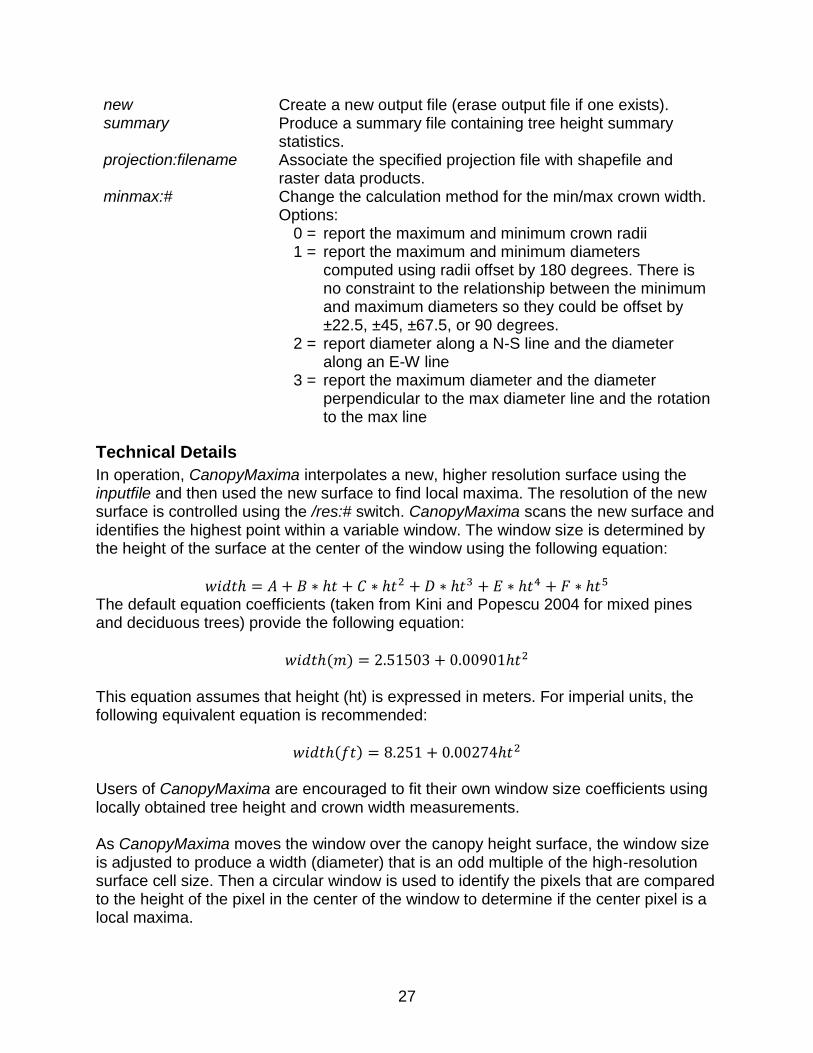
In operation, CanopyMaxima interpolates a new, higher resolution surface using the inputfile and then used the new surface to find local maxima. The resolution of the new surface is controlled using the /res:# switch. CanopyMaxima scans the new surface and identifies the highest point within a variable window. The window size is determined by the height of the surface at the center of the window using the following equation:

𝑤𝑖𝑑𝑡ℎ = 𝐴 + 𝐵 ∗ ℎ𝑡 + 𝐶 ∗ ℎ𝑡2 + 𝐷 ∗ ℎ𝑡3 + 𝐸 ∗ ℎ𝑡4 + 𝐹 ∗ ℎ𝑡5 The default equation coefficients (taken from Kini and Popescu 2004 for mixed pines and deciduous trees) provide the following equation:

𝑤𝑖𝑑𝑡ℎ(𝑚) = 2.51503 + 0.00901ℎ𝑡2 This equation assumes that height (ht) is expressed in meters. For imperial units, the following equivalent equation is recommended:

𝑤𝑖𝑑𝑡ℎ(𝑓𝑡) = 8.251 + 0.00274ℎ𝑡2 Users of CanopyMaxima are encouraged to fit their own window size coefficients using locally obtained tree height and crown width measurements. As CanopyMaxima moves the window over the canopy height surface, the window size is adjusted to produce a width (diameter) that is an odd multiple of the high-resolution surface cell size. Then a circular window is used to identify the pixels that are compared to the height of the pixel in the center of the window to determine if the center pixel is a local maxima.

28

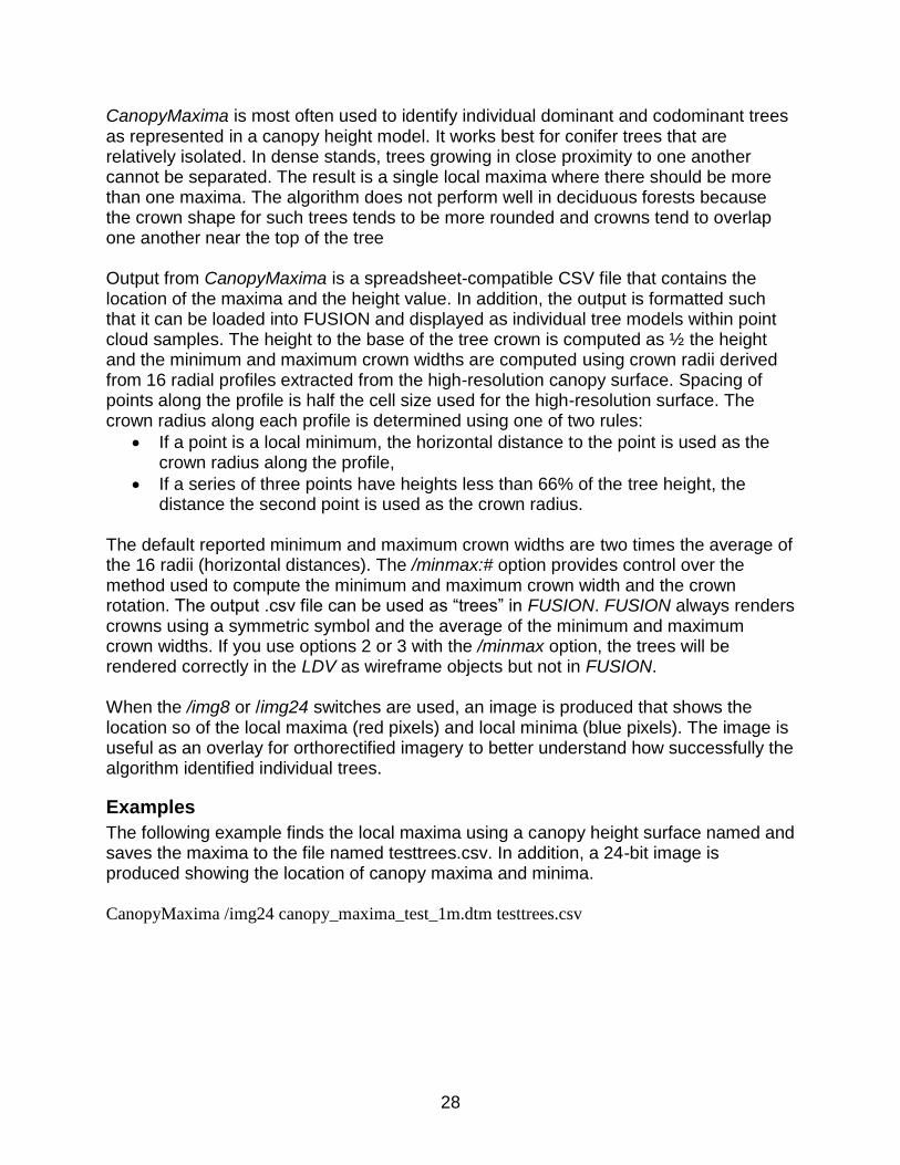
CanopyMaxima is most often used to identify individual dominant and codominant trees as represented in a canopy height model. It works best for conifer trees that are relatively isolated. In dense stands, trees growing in close proximity to one another cannot be separated. The result is a single local maxima where there should be more than one maxima. The algorithm does not perform well in deciduous forests because the crown shape for such trees tends to be more rounded and crowns tend to overlap one another near the top of the tree Output from CanopyMaxima is a spreadsheet-compatible CSV file that contains the location of the maxima and the height value. In addition, the output is formatted such that it can be loaded into FUSION and displayed as individual tree models within point cloud samples. The height to the base of the tree crown is computed as ½ the height and the minimum and maximum crown widths are computed using crown radii derived from 16 radial profiles extracted from the high-resolution canopy surface. Spacing of points along the profile is half the cell size used for the high-resolution surface. The crown radius along each profile is determined using one of two rules:

If a point is a local minimum, the horizontal distance to the point is used as the crown radius along the profile,

If a series of three points have heights less than 66% of the tree height, the distance the second point is used as the crown radius.

The default reported minimum and maximum crown widths are two times the average of the 16 radii (horizontal distances). The /minmax:# option provides control over the method used to compute the minimum and maximum crown width and the crown rotation. The output .csv file can be used as “trees” in FUSION. FUSION always renders crowns using a symmetric symbol and the average of the minimum and maximum crown widths. If you use options 2 or 3 with the /minmax option, the trees will be rendered correctly in the LDV as wireframe objects but not in FUSION. When the /img8 or /img24 switches are used, an image is produced that shows the location so of the local maxima (red pixels) and local minima (blue pixels). The image is useful as an overlay for orthorectified imagery to better understand how successfully the algorithm identified individual trees.

Examples

The following example finds the local maxima using a canopy height surface named and saves the maxima to the file named testtrees.csv. In addition, a 24-bit image is produced showing the location of canopy maxima and minima. CanopyMaxima /img24 canopy_maxima_test_1m.dtm testtrees.csv

29

CanopyModel

Overview

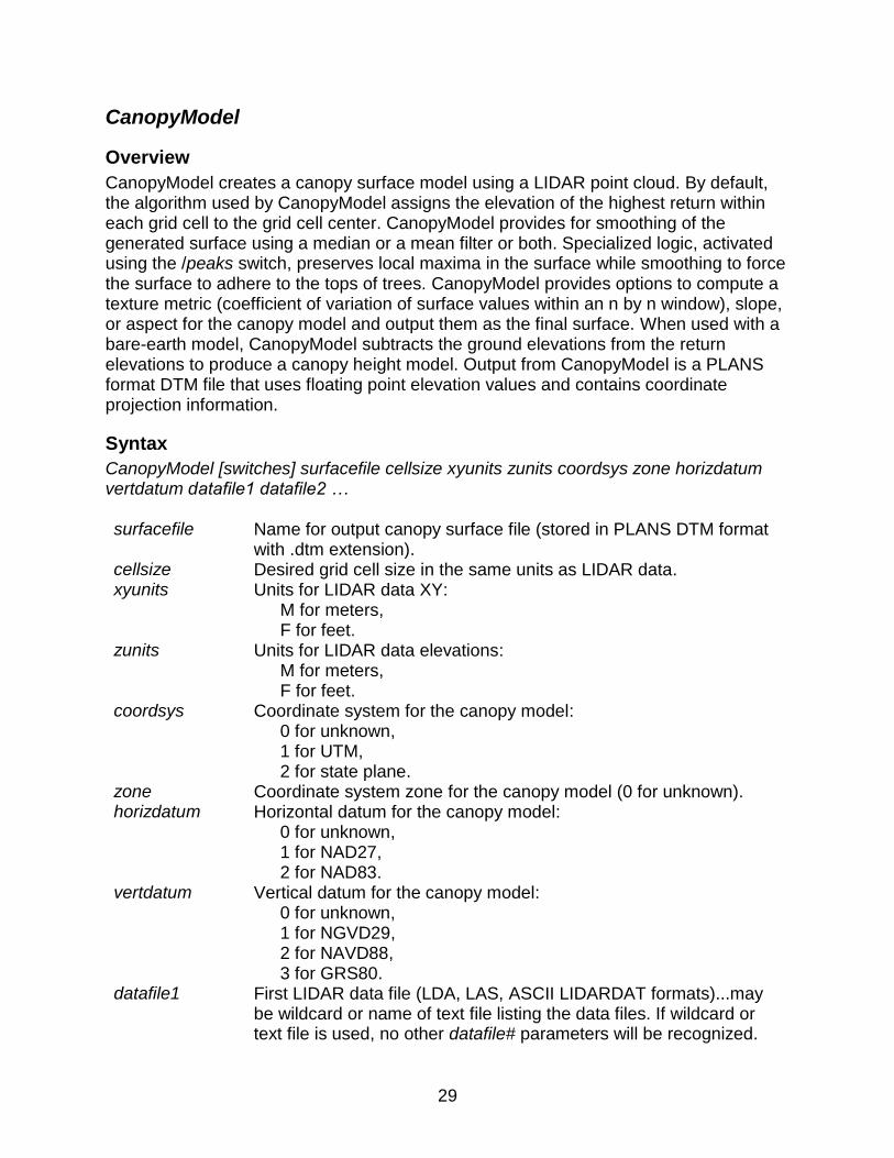
CanopyModel creates a canopy surface model using a LIDAR point cloud. By default, the algorithm used by CanopyModel assigns the elevation of the highest return within each grid cell to the grid cell center. CanopyModel provides for smoothing of the generated surface using a median or a mean filter or both. Specialized logic, activated using the /peaks switch, preserves local maxima in the surface while smoothing to force the surface to adhere to the tops of trees. CanopyModel provides options to compute a texture metric (coefficient of variation of surface values within an n by n window), slope, or aspect for the canopy model and output them as the final surface. When used with a bare-earth model, CanopyModel subtracts the ground elevations from the return elevations to produce a canopy height model. Output from CanopyModel is a PLANS format DTM file that uses floating point elevation values and contains coordinate projection information.

Syntax

CanopyModel [switches] surfacefile cellsize xyunits zunits coordsys zone horizdatum vertdatum datafile1 datafile2 … surfacefile Name for output canopy surface file (stored in PLANS DTM format

with .dtm extension). cellsize Desired grid cell size in the same units as LIDAR data. xyunits Units for LIDAR data XY:



coordsys Coordinate system for the canopy model: 0 for unknown, 1 for UTM, 2 for state plane.

zone Coordinate system zone for the canopy model (0 for unknown). horizdatum Horizontal datum for the canopy model:


vertdatum Vertical datum for the canopy model: 0 for unknown, 1 for NGVD29, 2 for NAVD88, 3 for GRS80.

datafile1 First LIDAR data file (LDA, LAS, ASCII LIDARDAT formats)...may be wildcard or name of text file listing the data files. If wildcard or text file is used, no other datafile# parameters will be recognized.

30

datafile2 Second LIDAR data file (LDA, LAS, ASCII LIDARDAT formats). Several data files can be specified. The limit depends on the length of each file name. When using multiple data files, it is best to use a wildcard for datafile1 or create a text file containing a list of the data files and specifying the list file as datafile1.

Switches

median:# Apply median filter to model using # by # neighbor window. smooth:# Apply mean filter to model using # by # neighbor window. texture:# Calculate the surface texture metric using # by # neighbor window. slope Calculate surface slope for the final surface. aspect Calculate surface aspect for the final surface. outlier:low,high Omit points with elevations below low and above high if used with a

bare-earth surface this option will omit points with heights below low or above high.

multiplier:# Multiply the output values by the constant (#). return:string Specifies the returns to be included in the sample (can include

A,1,2,3,4,5,6,7,8,9,F,L,O) Options are specified without commas (e.g. /return:123) For LAS files only: F indicates first and only returns, L indicates last of many returns.

class:string Used with LAS format files only. Specifies that only points with classification values listed are to be used when creating the canopy surface. Classification values should be separated by a comma e.g. (2,3,4,5) and can range from 0 to 31. If the first character of string is “~”, all classes except those listed will be used.

ground:file Use the specified bare-earth surface model(s) to normalize the LIDAR data. The file specifier can be a single file name, a “wildcard” specifier, or the name of a text file containing a list of model files (must have “.txt” extension). In operation, CanopyModel will determine which models are needed by examining the extents of the input point data.

ascii Write the output surface in ASCII raster format in addition to writing the surface in DTM format.

grid:X,Y,W,H Force the origin of the output grid to be (X,Y) instead of computing an origin from the data extents and force the grid to be W units wide and H units high...W and H will be rounded up to a multiple of cellsize.

gridxy:X1,Y1, X2,Y2

Force the origin of the output grid (lower left corner) to be (X1,Y1) instead of computing an origin from the data extents and force the upper right corner to be (X2, Y2). X2 and Y2 will be rounded up to a multiple of cellsize.

align:dtmfile Force alignment of the output grid to use the origin (lower left corner), width and height of the specified dtmfile. Behavior is the same as /gridxy except the X1,Y1,X2,Y2 parameters are read from the dtmfile.

31

extent:dtmfile Force the origin and extent of the output grid to match the lower left corner and extent of the specified PLANS format DTM file but adjust the origin to be an even multiple of the cell size and the width and height to be multiples of the cell size.

rasterorigin Offset the origin and adjust the extent of the surface so raster data products created using the surface will align with the extent specified with the /grid or /gridxy options. /rasterorigin is only used in conjunction with the /grid or /gridxy option.

surface Use the bare-earth surface model in conjunction with values specified in /outlier to omit points based on their height above the ground surface but create a surface that is not normalized relative to the bare-earth surface (the surface uses the point elevations).

peaks Preserve localized peaks in the final surface. Only useful with /median or /smooth.

pointcount Output the number of data points in each cell in addition to the canopy surface/height values. Counts are output in .DTM format. If there are no points for a cell, the elevation/height value for the cell is set to 999.0.

nofill Don’t fill holes in the surface model. In general, holes result from a lack of data within a cell. The default behavior is to fill holes in the interior of the surface model.

The order of the filter median and smooth switches is important. The first filter specified on the command line will be the first filter applied to the model (median or smooth). You cannot use /texture:#, /slope, and /aspect in combination.

Technical Details

CanopyModel uses the return with the highest elevation to compute the canopy surface model. If the /ground switch is used to produce a canopy height model, the ground elevation interpolated from the bare-earth surface model(s) is subtracted from the return elevation prior to determining the highest return value. It is important that the bare-earth model(s) truly represents the ground surface as any spikes due to residual vegetation returns in the point set used to create the bare-earth model will result in incorrect return heights and possible an incorrect canopy height model. The behavior of the /outlier switch depends on whether of not the /ground switch is used. Without the /ground switch, /outlier uses the return elevations and the low and high values to filter out returns based on the elevation. When used with the /ground switch, the height above ground is used to filter out returns. In general, the /outlier switch is more useful when used with the /ground switch. When either of the smoothing switches is used (/smooth or /median), an initial surface is computed using the highest return elevation for each cell. Then the initial surface is used to produce the final, smoothed surface. During the smoothing operation, the /peaks switch activates logic that compares the cell being modified to the other cells in

32

the smoothing window. If the target cell elevation is higher that all the neighboring cell elevations, its elevation will not be changed. CanopyModel can be used with bare-earth point sets to create a ground surface model that sits on top of the bare-earth points. In contrast, GridSurfaceCreate creates a surface that represents the average elevation for all points within a cell so the final surface it produces lies within the bare-earth point set. The /texture, /slope, and /aspect switches can be used with bare-earth point sets to produce descriptive layers for the ground surface. By default, CanopyModel fills “holes” in the surface where there were no points. The filling logic uses an eight-way search to find valid values on the surface and then uses a distance weighted average to compute values for the “holes”. This hole-filling logic can be disabled with the /nofill switch.

Examples

The following command will create a canopy surface model using a 5- by 5-meter grid. XY and elevation data are in meters. Data are referenced in the UTM coordinate system in zone 10. The horizontal datum is NAD83 and the vertical datum is NAVD88. Data files used to create the surface are listed in a text file named list.txt (shown below).

CanopyModel canopy_surface.dtm 5 m m 1 10 2 2 list.txt

The text file used to specify data file names contains the following:

000263.las

000264.las

000265.las

The following command will create the same canopy surface model but in this example, data files are listed explicitly on the command line.

CanopyModel canopy_surface.dtm 5 m m 1 10 2 2 000263.las 000264.las 000265.las

The following command will create the same canopy surface model but in this example, a wildcard specifier is used to reference the data files. When using wildcard specifiers, you need to make sure the specifier will result in the correct list of data files. You can test this by using the DIR command along with the specifier to verify the files that will be used to create the surface model (e.g., DIR *.las)

CanopyModel canopy_surface.dtm 5 m m 1 10 2 2 *.las

The following command line will create a canopy height model using the ground models contained in the current directory and the same data files as the precious example.

CanopyModel /ground:*.dtm canopy_height.dtm 5 m m 1 10 2 2 *.las

The following command will create the surface model and then apply a 5 by 5 cell median filter to smooth the surface (/median:5). Local maxima will be preserved in the surface (/peaks) to force the surface to adhere to the tops of trees.

33

CanopyModel /peaks /median:5 canopy_surface.dtm 5 m m 1 10 2 2 *.las

34

Catalog

Overview

Catalog produces a set of descriptive reports describing several important characteristics of LIDAR data sets. It is most often used to evaluate a new acquisition for internal quality, completeness of data coverage and return or pulse density. The primary output of Catalog is a web page that contains a summary of all data tiles evaluated including attribute summaries for each tile and overall summaries for the entire data set. Catalog provides options that will create the index files needed to use the LIDAR data with FUSION making it the logical first step in any analysis procedure. In addition to the web page, Catalog can produce images representing the coverage area, pulse and return densities, and intensity values for the entire acquisition. When data are stored in LAS format, Catalog includes a summary of points by classification code from the LAS data. All images produced by Catalog have associated world files so they can be used within FUSION to provide a frame-of-reference for analysis. Catalog also produces a FUSION hotspot file that provides specific details for each data tile in the FUSION environment.

Syntax

Catalog [switches] datafile [catalogfile] datafile LIDAR data file template or name of a text file containing

a list of file names (list file must have .txt extension). catalogfile Base name for the output catalog file (extensions will be

added). Switches

image Create image files showing the coverage area for each LIDAR file.

index Create LIDAR data file indexes if they don't already exist. newindex Create new LIDAR data file indexes for all files (even if

they already exist). drawtiles Draw data file extents and names on the intensity image. coverage Create one image that shows the nominal coverage area

for all data files included in the catalog. Also creates a FUSION hotspot file that provides details for each file in the catalog.

countreturns Adds columns in the CSV and HTML output to show the number of returns by return number for each data file and all data files combined. Runs that use this option can take much longer to process because Catalog has to read every point in the data files to count up the different returns. In theory, LAS files have this information in their header. However, file produced by some version of TerraScan do not have these fields populated with the actual number of data points by return number.

35

uselascounts Use the return counts stored in LAS file headers when /countreturns is specified to speed up the processing. Some software does not populate these items in the header so you have to make sure that the LAS header contains the return counts. When /countreturns is specified without /uselascounts or when processing data not stored in LAS format, the entire file is scanned to count the number of returns by return number.

rawcounts Outputs the number of returns (or first returns) in each cell. Used in conjunction with the /density and /firstdensity options. The output is in PLANS DTM format.

density:area,min,max Creates an image for all data files that shows the return density for the area represented by each pixel. area is the pixel area, min is the minimum acceptable point density per unit area, and max is the upper limit for the acceptable density range. Cells with point densities falling within the min-max range are colored green, cells with point densities below the minimum are colored red, and cells with densities above the maximum are colored blue.

firstdensity:area,min,max Creates an image for all data files that shows the density of first returns for the area represented by each pixel. area is the pixel area, min is the minimum acceptable point density per unit area, and max is the upper limit for the acceptable density range. Cells with first return densities falling within the min-max range are colored green, cells with point densities below the minimum are colored red, and cells with densities above the maximum are colored blue.

intensity:area,min,max Creates an intensity image for all data files using the average intensity for all first returns within each pixel. area is the pixel area, min is the minimum intensity value, and max is the maximum intensity value. A black to white color ramp is mapped to the range of intensity values defined by min and max. Ideally, min and max correspond to the range of intensity values present in the data. However, you may not always know the range of values for a given data set.

imageextent:minx, miny, maxx, maxy

Limit the area covered by image products to the specified extent.

bmp Save second copy of intensity image in BMP format with associated world file.

outlier:multiplier Performs a simple analysis to identify data tiles that might contain elevation outliers. The analysis marks tiles where the minimum, maximum, or range of elevations are outside the range defined by: mean value +- multiplier * std dev

36

The default multiplier is 2.0. noclasssummary Do not create a summary of return counts by LAS

classification values. This summary requires an extra read of the entire point data set and can add a significant amount of time to processing. If you don’t need the summary, use this option to speed things up.

class:string (LAS files only) Specifies that only points with classification values listed in string are to be included in the processing. Classification values should be separated by a comma e.g. (2,3,4,5). If the first character of string is “~”, all classes except those listed will be used. Older versions used /lasclass. /lasclass will still work but new scripts should use /class.

validate:maxreturn Produce report describing potential errors in point data files. Report will contain files with errors the might cause problems for other FUSION programs.

projection:filename Associate the specified projection file with image products. Make sure the projection file uses the one-line format and not a multiline format as some programs won’t recognize the multiline format files.

The "image" switch requires data file indexes. If indices do not already exist for all data files, use the "index" option to force their creation.

Technical Details

When creating intensity images, Catalog uses the average intensity for all returns within a cell to compute the grayscale color for the cell. This logic differs from that of the CreateImage program which uses the maximum intensity value for a cell. As a result, the images created by Catalog will differ from those created by CreateImage. The outlier detection logic in Catalog is very limited. In areas dominated by flat or relatively flat topography, the logic will usually identify data tiles with erroneous returns due to birds, multipathing, or system noise. In areas with steep topography, the logic will often miss such artifacts since the erroneous returns have elevations that may be outside the range in the vicinity of the return but are within the range for the entire data tile. The /density and /firstdensity switches should not be used with very small cell sizes (area <= 1 data unit). In general, LIDAR acquisitions result in uniformly spaced points on the ground. However, the spacing varies across the scan for most systems and using a cell that is too small will result in misleading results in the density images. When evaluating the density images, the user should consider the type of scan pattern used by the LIDAR system and the acquisition specifications. The point densities will vary depending on the position within the scan area, the total scan width (angle), pulse rate, and flying speed. For acquisitions with minimal side lap, densities at the edge of the

37

scan will be highly variable (for zig-zag scan patterns) when evaluated using a small cell size. The parameters for the /density and /firstdensity switches define the area of the cell and the thresholds used to classify pulse/return density for the cell. Cells used for these products are always square and the width/height is:

cellareacellsize

Density thresholds are expressed in pulses (or return) per square unit using the same units as those used for horizontal positions of the returns. The Table 1 shows equivalent density values when the horizontal units are meters and feet. The /image switch is obsolete. Use the /intensity switch instead. /image produces one image for each data tile and while this may be useful for small data sets containing only a few tiles, it produces a large number of images that must be examined when the data set is large with many tiles. In addition, /image requires data indexing prior to creation of the images. /intensity does not require index files and may be much faster when index files are not needed for other analysis tasks.

Table 1. Equivalent pulse (or return) densities for metric and imperial units of measure.

Density (pulses (or returns) per unit2) when horizontal units are:

Meters Feet

0.5 0.0464

1 0.0929

2 0.1858

4 0.3716

6 0.5574

8 0.7432

10 0.9291

12 1.1149

The /rawcounts switch produces raster output that provides detailed information describing the pulse (first return) and return density. The outputs are stored in the PLANS DTM data format and can be converted to ASCII raster format using the DTM2ASCII utility. The /rawcounts switch is used in conjunction with the /density and/or /firstdensity switches and the output products use the same grid cell size specified in these switches. If you plan to process the point data to produce metrics over large areas using scripts created by LTKProcessor, it is highly recommended that you use the /rawcounts switch in combination with /firstdensity switch and a fairly small cell size. This will produce a pulse density data layer that can be used by the LTKProcessor program to optimize the tile sizes used for processing. Cell size of around 10 m (100 m2) provide sufficient detail

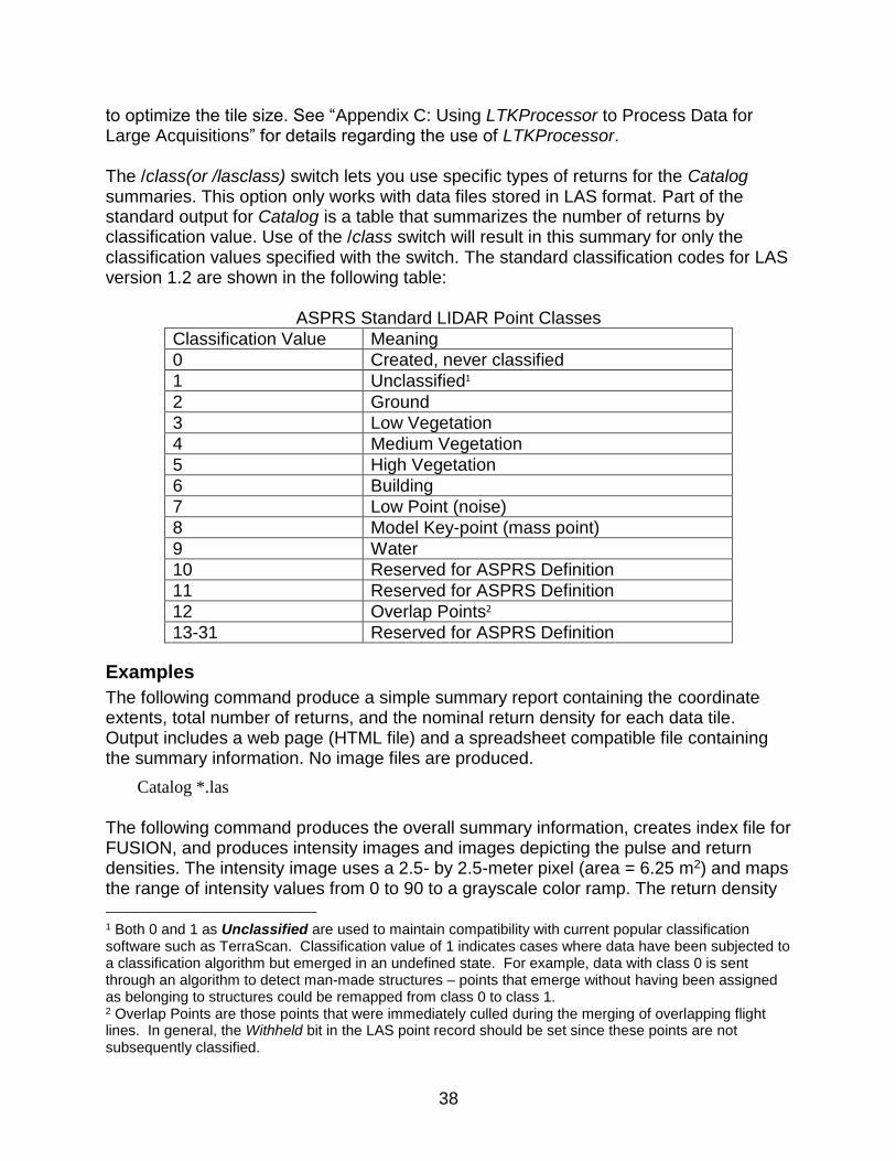
38

to optimize the tile size. See “Appendix C: Using LTKProcessor to Process Data for Large Acquisitions” for details regarding the use of LTKProcessor. The /class(or /lasclass) switch lets you use specific types of returns for the Catalog summaries. This option only works with data files stored in LAS format. Part of the standard output for Catalog is a table that summarizes the number of returns by classification value. Use of the /class switch will result in this summary for only the classification values specified with the switch. The standard classification codes for LAS version 1.2 are shown in the following table:

ASPRS Standard LIDAR Point Classes

Classification Value Meaning

0 Created, never classified

1 Unclassified1

2 Ground

3 Low Vegetation

4 Medium Vegetation

5 High Vegetation

6 Building

7 Low Point (noise)

8 Model Key-point (mass point)

9 Water

10 Reserved for ASPRS Definition


12 Overlap Points2

13-31 Reserved for ASPRS Definition

Examples

The following command produce a simple summary report containing the coordinate extents, total number of returns, and the nominal return density for each data tile. Output includes a web page (HTML file) and a spreadsheet compatible file containing the summary information. No image files are produced.

Catalog *.las

The following command produces the overall summary information, creates index file for FUSION, and produces intensity images and images depicting the pulse and return densities. The intensity image uses a 2.5- by 2.5-meter pixel (area = 6.25 m2) and maps the range of intensity values from 0 to 90 to a grayscale color ramp. The return density

1 Both 0 and 1 as Unclassified are used to maintain compatibility with current popular classification software such as TerraScan. Classification value of 1 indicates cases where data have been subjected to a classification algorithm but emerged in an undefined state. For example, data with class 0 is sent through an algorithm to detect man-made structures – points that emerge without having been assigned as belonging to structures could be remapped from class 0 to class 1. 2 Overlap Points are those points that were immediately culled during the merging of overlapping flight lines. In general, the Withheld bit in the LAS point record should be set since these points are not subsequently classified.

39

image uses a 5- by 5-meter pixel (area = 25 m2) and colors areas with less the 2 returns/m2 red, cells with 2 to 8 returns/m2 green and cells with more than 8 returns/m2 blue. The first return (or pulse) density image uses a 5- by 5-meter pixel (area = 25 m2) and colors areas with less the 1 pulse/m2 red, cells with 1 to 6 pulses/m2 green and cells with more than 6 pulses/m2 blue.

Catalog /index /intensity:6.25,0,90 /density:25,2,8 /firstdensity:25,1,6 *.las

40

ClipData

Overview

ClipData creates sub-samples of LIDAR data for various analysis tasks. The sub-sample can be round or rectangular and can be large or small. ClipData provides many of the same sampling options found in FUSION but it is not used by FUSION to perform subsampling of LIDAR data sets (FUSION has its own logic to accomplish this task). ClipData is often used to create sample of LIDAR returns around a specific point of interest such as a plot center or GPS measurement point. Subsequent analyses using programs like CloudMetrics facilitate comparing field data to LIDAR point cloud metrics. ClipData can extract a single sample or multiple samples using a single command. When creating several samples, it is much more efficient to use the optional syntax to clip several samples using a single command line. ClipData can also sub-sample data within the sample area using the elevation values for the returns. When used in conjunction with a bare-earth surface model, this logic allows for sampling a range of heights above ground within the sample area. ClipData can extract specific returns (1st, 2nd, etc) or first and last returns (LAS files only) for the sample area. This capability, when used with a large sample area, can extract specific returns from an entire data file. As part of the sampling process, ClipData can add (or subtract) a fixed elevation from each return elevation effecting adjusting the entire sample up or down. This capability, when used with a large sample area, can adjust entire data files up or down to help align data from different LIDAR acquisitions.

Syntax

ClipData [switches] InputSpecifier SampleFile [MinX MinY MaxX MaxY] InputSpecifier LIDAR data file template, name of a text file containing a list of file

names (must have .txt extension), or a FUSION Catalog CSV file. SampleFile Name for subsample file (extension will be added) or a text file

containing sample information for 1 or more samples. Each line in the text file should have the subsample filename and the MinX MinY MaxX MaxY values for the sample area separated by spaces or commas. The output filename cannot contain spaces.

MinX MinY Lower left corner of the sample area bounding box. MaxX MaxY Upper right corner of the sample area bounding box. Switches

shape:# Shape of the sample area: 0 rectangle, 1 circle.

decimate:# Skip # points between included points (must be > 0).

41

dtm:file ground:file

Use the specified bare-earth surface model to normalize the LIDAR data (subtract the bare-earth surface elevation from each lidar point elevation). Use with /zmin to include points above zmin or with /zmax to include points below zmax (file must be FUSION/PLANS format). file may be wildcard or text list file (extension .txt only) that specifies more than one ground surface model. In operation, only the models that cover the sample area will be used to normalize point data. The /ground switch was added to make ClipData more consistent with other LTK programs.

zmin:# Include points above # elevation. Use with /dtm to include points above # height.

zmax:# Include points below # elevation. Use with /dtm to include points below # height.

zpercent:# Include only the upper # percent of the points. If # is (-) only the lower # percent of the points. # can be -100 to +100.

height Convert point elevations into heights above ground using the specified DTM file. Always Used with /dtm.

timemin:# Include points with GPS times greater than # (LAS only). timemax:# Include points with GPS times less than or equal to # (LAS only).

Interpretation of # depends on the GPS time recorded in the LAS point records.

anglemin:# Include points with scan angles greater than # (LAS only). anglemax:# Include points with scan angles less than or equal to # (LAS only). zero Save subsample files that contain no data points. This is useful

when automating conversion and analysis tasks and expecting a subsample file every time ClipData is executed.

biaselev:# Add an elevation offset to every LIDAR point: # can be + or -. return:string Specifies the returns to be included in the sample. String can

include A,1,2,3,4,5,6,7,8,9,F,L. A includes all returns. For LAS files only: F indicates first and only returns, L indicates last of many returns. F and L will not work with non-LAS files.

class:string Used with LAS format files only. Specifies that only points with classification values listed are to be included in the subsample. Classification values should be separated by a comma e.g. (2,3,4,5) and can range from 0 to 31. If the first character of string is “~”, all classes except those listed will be used.

line:# LAS files only: Only include returns from the specified flight line. Line numbering varies by acquisition so you need to know your data to specify values for the flight line number.

noindex Do not use the data index files to access the data. This is useful when the order of the data points is important or when all returns for a single pulse need to stay together in the subsample file.

index Create FUSION index files for the SampleFile. lda Write output files using FUSION's LDA format when using LAS

input files. The default behavior after FUSION version 3.00 is to

42

write data in LAS format when the input data are in LAS format. When using input data in a format other than LAS, sample files are written in LDA format.

nooffset Produce an output point file that no longer has the correct geo-referencing. This is used when you need to work with the point cloud but cannot reveal the actual location of the features represented in the point cloud. This option modifies the header values in the LAS header for the output files.

precision:scaleX, scaleY,scaleZ

Control the scale factor used for X, Y, and Z values in output LAS files. These values will override the values in the source LAS files. There is rarely any need for the scale parameters to be smaller than 0.001.

Technical Details

ClipData uses FUSION index files, when they are available, to determine which data files need to be read to find returns within the sample area and to help reduce the number of points that need to be read within a given data file. Performance will be significantly slower if the data has not been indexed. Indexing is best accomplished using the Catalog program. If the /noindex switch is used, the index files will not be used. This is most often used when you need to preserve the original pulse and point order after the clipping process. When you specify the /index switch, ClipData creates FUSION index files for the sample file if it contains points. Having the index file significantly improves the performance of several LTK programs. The method used to compute the radius for round sample uses the average of the width and height of the sample area. This means that you should use sample corner coordinates that define a square area. Anything other than a square area will yield unexpected results when used with the /shape:1 switch. The /class switch allows you to include or omit returns based on the value stored in the LAS classification field. The LAS format specification includes a set of “standard” codes used to classify points. Some of the codes indicate specific features or structures and other indicate that the return is an outlier or point that should otherwise be ignored. The standard classification codes for LAS version 1.2 are shown in the following table:

ASPRS Standard LIDAR Point Classes


0 Created, never classified

1 Unclassified3

3 Both 0 and 1 as Unclassified are used to maintain compatibility with current popular classification software such as TerraScan. Classification value of 1 includes cases in which data have been subjected to a classification algorithm but emerged in an undefined state. For example, data with class 0 is sent

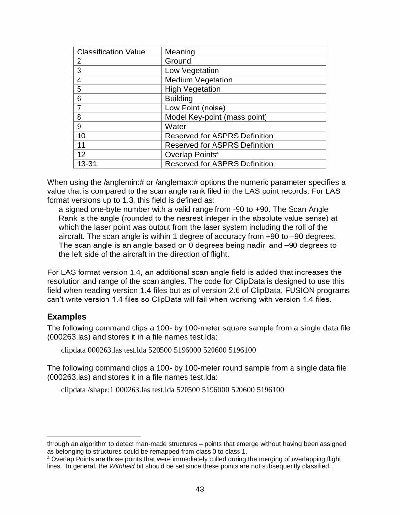
43


2 Ground

3 Low Vegetation

4 Medium Vegetation

5 High Vegetation

6 Building

7 Low Point (noise)

8 Model Key-point (mass point)

9 Water



12 Overlap Points4

13-31 Reserved for ASPRS Definition

When using the /anglemin:# or /anglemax:# options the numeric parameter specifies a value that is compared to the scan angle rank filed in the LAS point records. For LAS format versions up to 1.3, this field is defined as:

a signed one-byte number with a valid range from -90 to +90. The Scan Angle Rank is the angle (rounded to the nearest integer in the absolute value sense) at which the laser point was output from the laser system including the roll of the aircraft. The scan angle is within 1 degree of accuracy from +90 to –90 degrees. The scan angle is an angle based on 0 degrees being nadir, and –90 degrees to the left side of the aircraft in the direction of flight.

For LAS format version 1.4, an additional scan angle field is added that increases the resolution and range of the scan angles. The code for ClipData is designed to use this field when reading version 1.4 files but as of version 2.6 of ClipData, FUSION programs can’t write version 1.4 files so ClipData will fail when working with version 1.4 files.

Examples

The following command clips a 100- by 100-meter square sample from a single data file (000263.las) and stores it in a file names test.lda:

clipdata 000263.las test.lda 520500 5196000 520600 5196100

The following command clips a 100- by 100-meter round sample from a single data file (000263.las) and stores it in a file names test.lda:

clipdata /shape:1 000263.las test.lda 520500 5196000 520600 5196100

through an algorithm to detect man-made structures – points that emerge without having been assigned as belonging to structures could be remapped from class 0 to class 1. 4 Overlap Points are those points that were immediately culled during the merging of overlapping flight lines. In general, the Withheld bit should be set since these points are not subsequently classified.

44

ClipDTM

Overview

ClipDTM clips a portion of the gridded surface model and stores it in a new file. The extent of the clipped model is specified using the lower left and upper right corner coordinates.

Syntax

ClipDTM [switches] InputDTM OutputDTM MinX MinY MaxX MaxY InputDTM Name of the existing PLANS format DTM file to be clipped. OutputDTM Name for the new PLANS format DTM file. MinX MinY Lower left corner for the output DTM. MaxX MaxY Upper right corner for the output DTM. Switches

shrink Shrink the extent of the input model by the amounts specified by MinX MinY MaxX MaxY. MinX is removed from left side, MinY is removed from bottom, MaxX is removed from right side, and MaxY is removed from top.

Technical Details

When clipping a DTM, the lower left corner will be rounded down and the upper right corner will be rounded up to the nearest multiple of the InputDTM cell size. If the specified extent is outside the DTM area, the extent will be adjusted to match the extent of the InputDTM. The OutputDTM will use the same cell size and projection information as the InputDTM.

Examples

The following command line clips a subsample of the surface stored in FL_allarea.dtm and stores the resulting surface in clip.dtm:

ClipDTM FL_allarea.dtm clip.dtm 567320.4 7654984.2 569490.6 7655439.9

The following reduces the size of a surface stored in FL_allarea.dtm by 50 units on all sides and stores the result in shring.dtm:

ClipDTM /shrink FL_allarea.dtm cshrink.dtm 50.0 50.0 50.0 50.0

45

CloudMetrics

Overview

CloudMetrics computes a variety of statistical parameters describing a LIDAR data set. Metrics are computed using point elevations and intensity values (when available). In operation, CloudMetrics produces one record of output for each data file processed. Input can be a single LIDAR data file, a file template that uses DOS file specifier rules, a simple text file containing a list of LIDAR data file names, or a LIDAR data catalog produced by the Catalog utility. Output is appended to the specified output file unless the /new switch is used to force the creation of a new output data file. Output is formatted as a comma separated value (CSV) file that can be easily read by database, statistical, and MS-Excel programs. CloudMetrics is most often used with the output from the ClipData program to compute metrics that will be used for regression analysis in the case of plot-based LIDAR samples or for tree classification in the case of individual tree LIDAR samples.

Syntax

CloudMetrics [switches] InputDataSpecifier OutputFileName InputDataSpecifier LIDAR data file template, name of text file containing a list of

LIDAR data file names (must have .txt extension), or a catalog file produced by the Catalog utility.

OutputFileName Name for output file to contain cloud metrics (using a .csv will associate the files with MS-Excel).

Switches

above:# Compute various cover estimates using the specified heightbreak (#). See the technical detail for specific cover metrics that are computed.

new Creates a new output file and deletes any existing file with the same name. A header is written to the new output file.

firstinpulse Use only the first return for a pulse to compute metrics. Such returns may not always be labeled as return 1.

firstreturn Use only first returns to compute metrics. highpoint Produce a limited set of metrics that includes only the highest

return within the data file. subset Produce a limited set of metrics ([ID], #pts, Mean ht, Std dev ht,

75th percentile, cover). Must be used with the /above:# option. id Parse the data file name to create an identifier for the output

record. Data file names should include a number (e.g. sample003.lda) or the default identifier of 0 will be assigned to the file. The identifier is placed in the first column of the output record before the input file name.

46

rid Parse the data file name to create an identifier for the output record but start at the end of the filename. Data file names can include any characters but the end of the name should include a number preceded by a non-numeric character (e.g. 2017_01_13_sample003.las). The identifier is placed in the first column of the output record before the input file name.

minht:# Use only returns above # (use when data in the input data files have been normalized using a ground surface model. In older versions of CloudMetrics this switch was htmin.

maxht:# Use only returns below # (use when data is normalized to ground) to compute metrics. The maxht is not used when computing metrics related to the /strata or /intstrata options.

outlier:low,high Omit points with elevations below low and above high. When used with data that has been normalized using a ground surface, low and high are interpreted as heights above ground. You should use care when using /outlier:low,high with /minht and /maxht options. If the low value specified with /outlier is above the value specified with /minht, the value for /outlier will override the value specified for /minht. Similarly, if the high value specified with /outlier is less than the value specified for /maxht, the /outlier value will override the value for /maxht.

strata:[#,#,#,…] Count returns in various height strata. # gives the upper limit for each strata. Returns are counted if their height is >= the lower limit and < the upper limit. The first strata contains points < the first limit. The last strata contains points >= the last limit. Default strata: 0.15, 1.37, 5, 10, 20, 30.

intstrata:[#,#,#,…] Compute metrics using the intensity values in various height strata. Strata for intensity metrics are defined in the same way as the /strata option. Default strata: 0.15, 1.37.

kde:[window,mult] Compute the number of modes and minimum and maximum node using a kernal density estimator. Window is the width of a moving average smoothing window in data units and mult is a multiplier for the bandwidth parameter of the KDE. Default window is 2.5 and the multiplier is 1.0

rgb:color Compute intensity metrics using the color value from the RGB color for the returns. Valid with LAS version 1.2 and newer data files that contain RGB information for each return (point record types 2 and 3). Valid color values are R, G, or B.

relcover Obsolete as of CloudMetrics version 2.0. Metrics are computed as part of the default set of metrics. Compute the proportion of first (or all) returns above the mean and mode values.

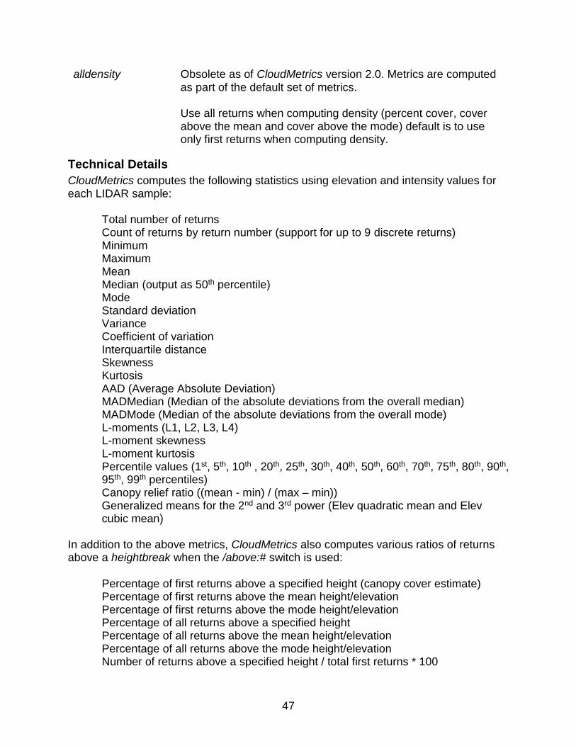
47

alldensity Obsolete as of CloudMetrics version 2.0. Metrics are computed as part of the default set of metrics. Use all returns when computing density (percent cover, cover above the mean and cover above the mode) default is to use only first returns when computing density.

Technical Details

CloudMetrics computes the following statistics using elevation and intensity values for each LIDAR sample:

Total number of returns Count of returns by return number (support for up to 9 discrete returns) Minimum Maximum Mean Median (output as 50th percentile) Mode Standard deviation Variance Coefficient of variation Interquartile distance Skewness Kurtosis AAD (Average Absolute Deviation) MADMedian (Median of the absolute deviations from the overall median) MADMode (Median of the absolute deviations from the overall mode) L-moments (L1, L2, L3, L4) L-moment skewness L-moment kurtosis Percentile values (1st, 5th, 10th , 20th, 25th, 30th, 40th, 50th, 60th, 70th, 75th, 80th, 90th, 95th, 99th percentiles) Canopy relief ratio ((mean - min) / (max – min)) Generalized means for the 2nd and 3rd power (Elev quadratic mean and Elev cubic mean)

In addition to the above metrics, CloudMetrics also computes various ratios of returns above a heightbreak when the /above:# switch is used:

Percentage of first returns above a specified height (canopy cover estimate) Percentage of first returns above the mean height/elevation Percentage of first returns above the mode height/elevation Percentage of all returns above a specified height Percentage of all returns above the mean height/elevation Percentage of all returns above the mode height/elevation Number of returns above a specified height / total first returns * 100

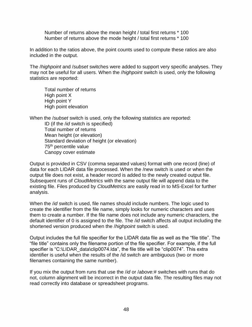
48

Number of returns above the mean height / total first returns * 100 Number of returns above the mode height / total first returns * 100

In addition to the ratios above, the point counts used to compute these ratios are also included in the output. The /highpoint and /subset switches were added to support very specific analyses. They may not be useful for all users. When the /highpoint switch is used, only the following statistics are reported:

Total number of returns High point X High point Y High point elevation

When the /subset switch is used, only the following statistics are reported:

ID (if the /id switch is specified) Total number of returns Mean height (or elevation) Standard deviation of height (or elevation) 75th percentile value Canopy cover estimate

Output is provided in CSV (comma separated values) format with one record (line) of data for each LIDAR data file processed. When the /new switch is used or when the output file does not exist, a header record is added to the newly created output file. Subsequent runs of CloudMetrics with the same output file will append data to the existing file. Files produced by CloudMetrics are easily read in to MS-Excel for further analysis. When the /id switch is used, file names should include numbers. The logic used to create the identifier from the file name, simply looks for numeric characters and uses them to create a number. If the file name does not include any numeric characters, the default identifier of 0 is assigned to the file. The /id switch affects all output including the shortened version produced when the /highpoint switch is used. Output includes the full file specifier for the LIDAR data file as well as the “file title”. The “file title” contains only the filename portion of the file specifier. For example, if the full specifier is “C:\LIDAR_data\clip0074.lda”, the file title will be “clip0074”. This extra identifier is useful when the results of the /id switch are ambiguous (two or more filenames containing the same number). If you mix the output from runs that use the /id or /above:# switches with runs that do not, column alignment will be incorrect in the output data file. The resulting files may not read correctly into database or spreadsheet programs.

49

The cover value computed in CloudMetrics when the /above:# switch is used is computed as follows: (# of first returns > heightbreak) / (total number of first returns) Figure 3 illustrates the concept of estimating canopy cover using LIDAR first return data: In Figure 3, overstory canopy is defined as any vegetation greater than the height break (3 meters in this example) above the ground. Of the 21 LIDAR pulses that enter the canopy, 16 first returns are recorded above the 3-meter threshold. The LIDAR-based overstory cover estimate would be computed as 16/21 or 76 percent. The height break is specified with the /above:# switch.

Figure 3. Schematic of the cover calculation process.

The /firstinpulse and /firstreturn switches cause different behaviors. When /firstinpulse is used, logic tries to figure out which returns represent the first return for a each laser pulse. When data are clipped into tiles for delivery or into samples representing specific areas (e.g., forest measurement plots), returns for a specific pulse may be split between two data files. The result is that the return labeled as the first return for a pulse may not be included in the sample. When /firstinpulse is specified, the first return for each pulse is used to compute metrics even if it is not labeled as return 1. When /firstreturn is used, only returns identified as the first return (return number 1) are used to compute metrics. The percentile values are computed using the following method (http://www.resacorp.com/method_5.htm, last accessed August 2016):

http://www.resacorp.com/method_5.htm

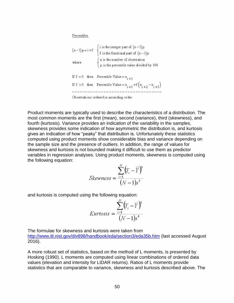
50

Product moments are typically used to describe the characteristics of a distribution. The most common moments are the first (mean), second (variance), third (skewness), and fourth (kurtosis). Variance provides an indication of the variability in the samples, skewness provides some indication of how asymmetric the distribution is, and kurtosis gives an indication of how “peaky” that distribution is. Unfortunately these statistics computed using product moments show considerable bias and variance depending on the sample size and the presence of outliers. In addition, the range of values for skewness and kurtosis is not bounded making it difficult to use them as predictor variables in regression analyses. Using product moments, skewness is computed using the following equation:

and kurtosis is computed using the following equation:

The formulae for skewness and kurtosis were taken from http://www.itl.nist.gov/div898/handbook/eda/section3/eda35b.htm (last accessed August 2016). A more robust set of statistics, based on the method of L moments, is presented by Hosking (1990). L moments are computed using linear combinations of ordered data values (elevation and intensity for LIDAR returns). Ratios of L moments provide statistics that are comparable to variance, skewness and kurtosis described above. The

http://www.itl.nist.gov/div898/handbook/eda/section3/eda35b.htm

51

first four L moments (𝜆1, 𝜆2, 𝜆3, 𝜆4) are estimated using the direct sample estimators proposed by Wang (1996) and the L moment ratios corresponding to coefficient of variation (𝜏2), skewness (𝜏3), and kurtosis (𝜏4) are computed as follows (theoretical parameter ranges are also shown):

𝜏2 =𝜆2

𝜆1 0 < 𝜏2 < 1

𝜏3 =𝜆3

𝜆2 −1 < 𝜏3 < 1

𝜏4 =𝜆4

𝜆2

1

4(5𝜏3

2 − 1) ≤ 𝜏4 < 1

Average Absolute Deviation (AAD) is computed using the following equation:

Median absolute deviation from the median (MADMedian) is a robust estimator of the variability within a data sample. MADMedian is compute using the following equation:

𝑀𝐴𝐷𝑚𝑒𝑑𝑖𝑎𝑛 = 𝑚𝑒𝑑𝑖𝑎𝑛𝑖(|𝑋𝑖 − 𝑚𝑒𝑑𝑖𝑎𝑛𝑗(𝑋𝑗)|)

Median absolute deviation from the mode (MADMode) is another estimator of variability within a data sample. MADMode is computed using the following equation:

𝑀𝐴𝐷𝑚𝑜𝑑𝑒 = 𝑚𝑒𝑑𝑖𝑎𝑛𝑖(|𝑋𝑖 − 𝑚𝑜𝑑𝑒𝑗(𝑋𝑗)|)

Generalized means for the 2nd (Elev quadratic mean) and the 3rd (Elev cubic mean) power are computed using the following equation with p=2 and p=3 respectively:

𝑀𝑝 = (1

𝑛∑ 𝑥𝑖

𝑝

𝑛

𝑖=1

)

1𝑝

Mode is computed by dividing the data range (either elevation or intensity) into 64 classes and counting the number of returns in each class. The mode is then the class with the largest number of values. In cases where several classes have the same number of returns, the mode will be the class with the lowest value. Mode values are not necessarily unique since several values may occur with equal frequency. In addition, the precision of the mode estimate varies depending on the height range of the point data. Data with a smaller range of heights will have a more precise value for the mode while data with a larger range will have a less precise value. This occurs because 64 bins are always used to partition the data regardless of the height range of the data.

52

For these reasons, the mode should be used with caution. Mean or median may be better measures of the central tendency of the elevation or intensity values in a point cloud. The /strata and /intstrata options compute a subset of the metrics for points within the specified height bands. The default strata heights (0.15, 1.37, 5, 10, 20, 30 for /strata and 0.15, 1.37 for /intstrata) are provided to simplify use of these options. The following metrics are computed for each height band when /strata is used:

Number of returns in the strata Minimum elevation/height for the points in the strata Maximum elevation/height for the points in the strata Average elevation/height for the points in the strata Mode value for elevation/height for the points in the strata Median value for elevation/height for the points in the strata Standard deviation of the elevation/height for the points in the strata Skewness of the elevations/heights for the points in the strata Kurtosis of the elevations/heights for the points in the strata

When /intstrata is used, the same metrics are computed using the intensity values for the points in each height band. The /kde option uses kernel density estimation (KDE) with a Gaussian kernel to construct a probability density function for the point heights in the sample. KDE is essentially a data smoothing approach used to make inferences regarding the distribution of target elements based on the collection of returns in the sample. Outputs from the KDE approach are the number of modes (peaks), the minimum and maximum mode values (peak heights), and the range between the minimum and maximum mode values. The formula for the kernel density estimator with a Gaussian kernel is:

�̂�(𝑥) = 1

𝑁√2𝜋ℎ∑ 𝑒

−((𝑥−𝑥𝑖)2

2ℎ2 )𝑁

𝑖=1

The x values range over the extent of the point heights. The number of samples, N, is fixed at 512. xi is the height of the i th point. The smoothing constant (h) is calculated using Silverman’s rule-of-thumb (Silverman 1986, p 48, eqn 3.31):

ℎ = 0.9 ∗ 𝐴 ∗ 𝑁−15

where:

𝐴 =min (𝑠𝑡𝑑 𝑑𝑒𝑣, 𝑖𝑛𝑡𝑒𝑟𝑞𝑢𝑎𝑟𝑡𝑖𝑙𝑒 𝑑𝑖𝑠𝑡𝑎𝑛𝑐𝑒)

1.34

53

The smoothing constant is multiplied by the optional mult parameter. Prior to peak detection, the probability density function is smoothed using a moving window average with a window size specified by the optional window parameter. A value of 0.0 for the window parameter disables the smoothing logic so peaks are derived from the “raw” density function. Peaks are detected by looking for changes from a positive slope to a negative slope. Use caution when using the /RGB switch since the output columns for the Intensity, R, G, and B metrics are the same. It is very easy to mix outputs from runs intended to compute the metrics using the color values with each other and those where the actual intensity value was used to compute metrics.

Examples

The following command line would generate metrics for all LIDAR data files in the current directory and store them in a CSV file named metrics.csv. If the output file, metrics.csv, already exists, output will be appended to the file and no header will be added to the file.

cloudmetrics *.lda metrics.csv

The following command would generate metrics for all LIDAR data files in the current directory and store them in a new file named metrics.csv. If the output file, metrics.csv, already exists, it will be overwritten and a new header line will be added before any metrics are written. The names of individual data files will be used to create an identifier that will be added as the first column of data in the output file.

cloudmetrics /new /id *.lda metrics.csv

54

Cover

Overview

Cover computes estimates of canopy closure using a grid. Output values for cover estimates range from 0.0 to 100.0 percent. Canopy closure us defined as the number of returns over a specified height threshold divided by the total number of returns within each cell. In addition, Cover can compute the proportion of pulses that are close to a bare-ground surface model to help assess canopy penetration by the laser scanner. Wit the addition of an upper height limit, Cover can compute the proportion of returns falling within specific height ranges providing estimates of relative vegetation density for various height strata.

Syntax

Cover [switches] groundfile coverfile heightbreak cellsize xyunits zunits coordsys zone horizdatum vertdatum datafile1 datafile2... groundfile File specifier for the bare-ground surface model used to normalize all

return elevations. The file specifier can be a single file name, a “wildcard” specifier, or the name of a text file containing a list of model files (must have “.txt” extension). In operation, Cover will determine which models are needed by examining the extents of the input point data.

coverfile Name for the cover data file. The cover data is stored in the PLANS DTM format using floating point values.

heightbreak Height break for the cover calculation. cellsize Grid cell size for the cover data. xyunits Units for LIDAR data XY:



coordsys Coordinate system for the cover data: 0 for unknown, 1 for UTM, 2 for state plane.

zone Coordinate system zone for the cover data (0 for unknown). horizdatum Horizontal datum for the cover data:


vertdatum Vertical datum for the cover data: 0 for unknown, 1 for NGVD29, 2 for NAVD88, 3 for GRS80.

55



Switches

all Use all returns to calculate the cover data. The default is to use only first returns.


penetration Compute the proportion of returns close to the ground surface by counting the number of returns within +-heightbreak units of the ground.

upper:# Use an upperlimit when computing the cover value. This allows you to calculate the proportion of returns between the heightbreak and upperlimit.

Technical Details

When computing cover, returns with elevations <= heightbreak are counted. When computing cover with an upper height limit, returns with elevations (or height above ground) >= heightbreak and <= upperlimit are counted. When computing penetration, returns with heights above ground >= -heightbreak and <= +heightbreak are counted. Cover values are computed as described in the CloudMetrics section. The specific equation when the /all switch is NOT used is:

(# of 1st returns > heightbreak) / (total number of 1st returns) When the /all switch is used the equation is:

(# of returns > heightbreak) / (total number of returns) To produce cover estimates that are meaningful, the cell size must be larger that individual tree crowns. With small cell sizes (less than 5 meters) the distribution of cover values of a large area tends to be heavy on values near 0 and 100 because each cell serves to test for the presence or absence of a tree instead of providing a reasonable sample area for assessing vegetation cover. For most forest types, cell sizes of 15-meter or larger produce good results.

56

By default, Cover uses only first returns to compute cover. All returns can be used by specifying the /all switch. Figure 3 illustrates the concept of estimating canopy cover using LIDAR first return data:

When not using the /all switch, the number of first returns will only be reported for data files that are .LDA files that have not been indexed or ASCII text files. The number of first returns will not be reported for indexed .LDA or .LAS files. This is due to the ability to obtain the data extent for a file from either the index file header or the .LAS file header making a point-by-point read of the file unnecessary. Only first returns will be used to compute the cover or penetration data regardless of the file format.

Examples

The following command creates cover estimates using a 15- by 15-meter grid and a heightbreak of 3 meters. Data are in the UTM coordinate system, zone 10, with units for both horizontal values and elevations of meters. The data uses the NAD83 horizontal and NAVD88 vertical datums.

Cover 000263_ground_1m.dtm 000263_cover_15m.dtm 3 15 m m 1 10 2 2 000263.las

The following command computes the proportion of the pulses that penetrate canopy to reach the ground using a 30- by 30-meter grid and a ground tolerance of 2 meters.

Cover /penetration 000263_ground_1m.dtm 000263_grndpen_30m.dtm 2 30 m m 1 10 2 2

000263.las

57

CSV2Grid

Overview

CSV2Grid converts data stored in comma separated value (CSV) format into ASCII raster format. In operation, users specify the column from the CSV file to convert. CSV2Grid expects a header file that corresponds to the input file. The header file name is formed from the input file name by appending the text “_ascii_header” and changing the extension to “.txt”. Normally, the CSV files used with CSV2Grid are produced by GridMetrics.

Syntax

CSV2GRID [switches] inputfile column outputfile inputfile Name of the input CSV file. This file is normally output from

GridMetrics. column Column number for the values to populate the grid file (column

numbers start with 1). outputfile Name for the output ASCII raster file. Switches

multiplier:# Multiply all data values by the constant (#). ndzero:# If the value in the target column is NODATA, look at the value in

column # and, if it is a valid value (not NODATA), change the value for the target column to 0.0 for output to the ASCII grid file. This option is useful when the ASCII grid file will be used for further analysis in GIS or statistical packages.

Technical Details

CSV2Grid must be able to find the header file associated with inputfile. The header contains the ASCII raster grid header and is copied directly into the outputfile. For use with ArcInfo, the outputfile should be named using an extension of “.asc”.

Examples

The following command converts the data from the third column of the CSV file named return_density.csv into ASCII raster file named return_density.asc:

CSV2Grid return_density.csv 3 return_density.asc

58

DensityMetrics

Overview

DensityMetrics is designed to output a series of grids where each grid contains density information for a specific range of heights above ground. Densities are reported as the proportion of the returns within the layer. Output consists of a CSV file with columns that correspond to the layers and PLANS format DTM files (one for each layer) containing the point density information.

Syntax

DensityMetrics [switches] groundfile cellsize slicethickness outputfile datafile1 datafile2 ... datafileN groundfile File specifier for the bare-ground surface model used to normalize

all return elevations. The file specifier can be a single file name, a “wildcard” specifier, or the name of a text file containing a list of model files (must have “.txt” extension). In operation, DemsityMetrics will determine which models are needed by examining the extents of the input point data.

cellsize Desired grid cell size for the point density data in the same units as the point data.

slicethickness Thickness for each “slice” in the same units as the point elevations. outputfile Base file name for output. Metrics are stored in CSV format with the

extension .csv unless the /nocsv switch is specified, Other outputs are stored in files named using the base name and additional descriptive information.



Switches

outlier:low,high Ignore points with elevations below low and above high. Low and high are interpreted as heights above ground as defined by the groundfile.

maxsliceht:high Limit the range of height slices to 0 to high. nocsv Do not create a CSV output file for cell metrics. class:string Used with LAS format files only. Specifies that only points with

classification values listed are to be included when computing density metrics. Classification values should be separated by a comma e.g. (2,3,4,5) and can range from 0 to 31. If the first character of string is “~”, all classes except those listed will be used.

59

first Use only first returns to compute all metrics. The default is to use all returns to compute the metrics.

slices:#,#,#,… Use specific slice height breaks rather that evenly spaced breaks based on the range of heights in the data. You can specify a maximum of 64 slice heights. The first slice always starts at 0.0. Slice heights must be specified in ascending order. The highest slice will contain the count of all points with heights greater than or equal to the last height break. Slice height ranges are defined as: lower ht <= point height < upper height.


gridxy:X1,Y1, X2,Y2



buffer:width Add an analysis buffer of the specified width (same units as LIDAR data) around the data extent when computing metrics but only output metrics for the area specified via /grid, /gridxy, or /align. When /buffer is used without one of these options, metrics are output for an area that is inside the actual extent of the return data as metrics within the buffer area are not output.

cellbuffer:width Add an analysis buffer specified as the number of extra rows and columns around the data extent when computing metrics but only output metrics for the area specified via /grid, /gridxy, or /align. When /cellbuffer is used without one of these options, metrics are output for an area that is inside the actual extent of the return data as metrics for the buffer area are not output.

Technical Details

The CSV files output (CSV file output is suppressed if the /nocsv switch is specified) from DensityMetrics include the row and column of the cell (0, 0 is upper left row/col), the maximum return height for the cell, the total number of returns in the cell, and the number of returns within each height slice. Returns are considered “in a slice” if the height above ground is greater than or equal to the base height for the slice and less than the upper height for the slice. If a return is below the ground surface, the elevation is changed to 0.0 and it is counted in the lowest slice. A text file that contains the header information for the CSV file is included for use with CSV2Grid. The header file is named using the name of the output file with the phrase “_ascii_header” appended and the extension “.txt”.

60

When the /grid, /gridxy, or /align switches are used, DensityMetrics tests the extent of indexed LDA files and LAS files to see if any points in the file fall within the specified grid area. If the file extent and the grid area do not overlap, the file is skipped. This allows you to use DensityMetrics to compute statistics for small sample areas without identifying the specific data tiles that contain the sample. You specify the desired sample area and all data tiles and let DensityMetrics figure out which tiles contain points within the sample area. If you are not using indexed LDA files or LAS files, such an approach will result in slow performance as every point in all tiles must be read and tested to see if it is within the grid area. A PLANS format surface file is produced for each height slice. The cell values in the surface are the proportion of returns within the slice expressed as a percentage ranging from 0 to 100. The number of slices that can be used in DensityMetrics depends on the extent of the data, the cell size, and the amount of available memory. For processing efficiency, DensityMetrics must hold the point count data for all slices in memory. Specifying a small slicethickness without using a maxsliceht can result in too many slices in which case, DensityMetrics will fail.

Examples

The following command creates density metrics for the data stored in tile0023.lda and outputs both a CSV and PLANS surface files. Height slices are 3 meter in thickness and return densities are summed using a 5- by 5-meter cell.

DensityMetrics bareearth.dtm 5 3 tile0023_density.csv tile0023.lda

61

DTM2ASCII

Overview

DTM2ASC converts data stored in the PLANS DTM format into ASCII raster files. Such files can be imported into GIS software such as ArcInfo. DTM2ASCII provides the same functionality as the Tools…Terrain model…Export model… menu option in FUSION.

Syntax

DTM2ASCII [switches] inputfile [outputfile] inputfile Name of the PLANS DTM file to be converted into ASCII raster format. outputfile Name for the converted file. If outputfile is omitted, the output file name

will be constructed from the inputfile name and the extension .asc. When the csv switch is specified, the default extension used to construct an output file name is .csv.

Switches

csv Output data values in comma separated value format. Header is the column number. Data are arranged in rows with the northern-most row first in the file.

raster Interpret the DTM points as the attribute for a cell and adjust the origin of the ASCII grid file so that the lower left data point is the center of the lower left grid cell. For almost all applications, you should use the /raster option.

multiplier:# Multiply the output values by the constant (#).

Technical Details

If the PLANS DTM file uses floating point data values, the ASCII raster file will use floating point values with 6 digits to the right of the decimal point. If the PLANS DTM uses integer values, the ASCII raster file will use integer values. NODATA will be labeled with a value of -9999.0000 for floating point files or -9999 for integer files.

Examples

The following command will convert a PLANS DTM file into ASCII raster format. The output file will be named 000263_ground_1m.asc.

DTM2ASCII /raster 000263_ground_1m.dtm

62

DTM2ENVI

Overview

DTM2ENVI converts data stored in the PLANS DTM format into ENVI standard format raster files. Such files can be imported into GIS software such as ENVI and ArcInfo.

Syntax

DTM2ENVI [switches] inputfile [outputfile] inputfile Name of the PLANS DTM file to be converted into ASCII raster format. outputfile Name for the converted file. If outputfile is omitted, the output file name

will be constructed from the inputfile name and the extension .nvi. The associated ENVI header file is named by appending “.hdr” to the inputfile name.

Switches

south Specifies that data are located in the southern hemisphere.

Technical Details

The ENVI data file is created using the same numeric format as the PLANS DTM file. All PLANS DTM data types are supported. Geo-referencing information is included in the ENVI header file using the “map info” tag. Areas in the DTM grid that have no data will be “marked” with a value of -9999.0 in the ENVI format file and the appropriate value will be included in the “data ignore value” tag in the ENVI header file.

Examples

The following command will convert a PLANS DTM file into ENVI standard raster format. The output file will be named 000263_ground_1m.nvi and the associated header file will be named 000263_ground_1m.nvi.hdr.

DTM2ENVI 000263_ground_1m.dtm

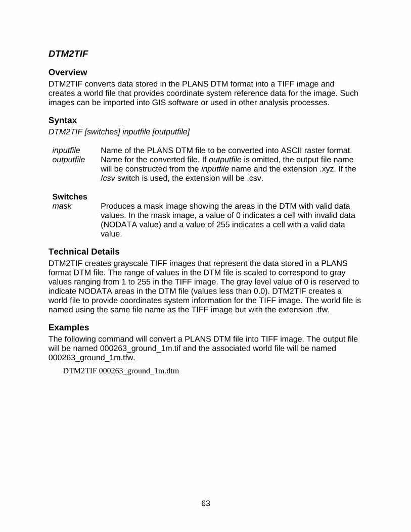
63

DTM2TIF

Overview

DTM2TIF converts data stored in the PLANS DTM format into a TIFF image and creates a world file that provides coordinate system reference data for the image. Such images can be imported into GIS software or used in other analysis processes.

Syntax

DTM2TIF [switches] inputfile [outputfile] inputfile Name of the PLANS DTM file to be converted into ASCII raster format. outputfile Name for the converted file. If outputfile is omitted, the output file name

will be constructed from the inputfile name and the extension .xyz. If the /csv switch is used, the extension will be .csv.

Switches

mask Produces a mask image showing the areas in the DTM with valid data values. In the mask image, a value of 0 indicates a cell with invalid data (NODATA value) and a value of 255 indicates a cell with a valid data value.

Technical Details

DTM2TIF creates grayscale TIFF images that represent the data stored in a PLANS format DTM file. The range of values in the DTM file is scaled to correspond to gray values ranging from 1 to 255 in the TIFF image. The gray level value of 0 is reserved to indicate NODATA areas in the DTM file (values less than 0.0). DTM2TIF creates a world file to provide coordinates system information for the TIFF image. The world file is named using the same file name as the TIFF image but with the extension .tfw.

Examples

The following command will convert a PLANS DTM file into TIFF image. The output file will be named 000263_ground_1m.tif and the associated world file will be named 000263_ground_1m.tfw.

DTM2TIF 000263_ground_1m.dtm

64

DTM2XYZ

Overview

DTM2XYZ converts data stored in the PLANS DTM format into ASCII text files containing XYZ points. Such files can be imported into GIS software as point data with the elevation as an attribute or used in other analysis processes.

Syntax

DTM2XYZ [switches] inputfile [outputfile] inputfile Name of the PLANS DTM file to be converted into ASCII raster format. outputfile Name for the converted file. If outputfile is omitted, the output file name

will be constructed from the inputfile name and the extension .xyz. If the /csv switch is used, the extension will be .csv.

Switches

csv Output XYZ points in comma separated value format (CSV). If /csv is used with no outputfile, an extension of .csv will be used to form the output file name.

void Output points from DTM with NODATA value (default is to omit). NODATA value is -9999.0 for the elevation.

noheader Do not include the column headings in CSV output files. Ignored if /csv is not used

Technical Details

The XYZ point file consists of one record for each grid point. Each record contains the X, Y, and elevation for the DTM grid point. If creating an ASCII text file, the values are separated by spaces and if creating a CSV format file, by commas. For CSV files, the first line contains column labels unless the /noheader switch is specified.

Examples

The following command will convert a PLANS DTM file into XYZ points stored in ASCII format. The output file will be named 000263_ground_1m.xyz.

DTM2XYZ 000263_ground_1m.dtm

65

DTMDescribe

Overview

DTMDescribe reads header information for PLANS format DTM files and outputs the information to an ASCII text file compatible with most spreadsheet and database programs. DTMDescribe can provide information for a single file or multiple files.

Syntax

DTMDescribe [switches] inputfile outputfile inputfile DTM file name, DTM file template, or name of a text file containing a list

of file names (must have .txt extension). outputfile Name for the output ASCII CSV file. If no extension is provided, an

extension (.csv) will be added. Switches

The standard FUSION-LTK toolkit switches are supported,

Technical Details

DTMDescribe produced output files in comma separated value (CSV) format and includes column labels in the first line of the file. The following header information from the DTM file is included in the CSV file:

File name Descriptive name Origin (X, Y) Upper right (X, Y) Number of columns Number of rows Column spacing Row spacing Minimum data value Maximum data value Horizontal units Vertical units Variable type Coordinate system Coordinate zone Horizontal datum Vertical datum

Examples

The following example outputs the header information for all DTM files in the current directory to the CSV file named summary.csv.

DTMDescribe *.dtm summary.csv

66

DTMHeader

Overview

DTMHeader is an interactive program. It is described in the Command Line Utility section because it provides a means to examine and modify PLANS DTM file header information. DTMHeader allows you to easily view and change the header information for a PLANS DTM file. To make it most convenient, associate the .dtm extension with DTMHeader so you can simply double-click a .dtm file to view the header. The values in the header that can be modified are:

Planimetric units, Elevation units, Descriptive name, Coordinate system and zone, Horizontal datum, Vertical datum.

Syntax

DTMHeader [filename] filename Name of the PLANS DTM file to be examined.

Technical Details

The standard FUSION-LTK switches are not recognized by DTMHeader and it does not write entries to the FUSION-LTK master log file. When run with no filename, DTMHeader allows the user to interactively select a DTM file for examination. If you make changes to a header value, you will be prompted to save the file when you exit the program or when you try to access a different DTM file.

67

FilterData

Overview

FilterData applies various filters to return data files to produce new return data files with only the returns that meet the filter requirements. The most common application for FilterType is to remove “outliers” from return data files. Other filter options overlay the return data with a user-specified grid and produce output return files that contain only the returns with the minimum or maximum elevation for each grid cell.

Syntax

FilterData [switches] FilterType FilterParms WindowSize OutputFile DataFile FilterType Filtering algorithm used to remove returns from the DataFile(s).

The following options (by name) are supported: outlier removes returns above or below the mean

elevation plus or minus FilterParms * standard deviation of the elevations

outlier2 More robust outlier removal (experimental) minimum removes all returns except the return with the

minimum elevation maximum removes all returns except the return with the

maximum elevation FilterParms Parameters specific to the filtering method. For outlier this is the

multiplier applied to the standard deviation. For minimum and maximum, FilterParms is ignored (but a value must be included on the command line...use 0)

WindowSize Size of the window used to compute the standard deviation of elevations or the minimum/maximum return

OutputFile Name of the output file. If any part of the name includes spaces, include the entire name in double quotation marks

DataFile LIDAR data file name or template or name of a text file containing a list of file names (list file must have .txt extension).

Switches

index Create FUSION index files for the output file. minsd:# Minimum standard deviation for points within a comparison

window for filtering to take place. Default is 1.0 (same units as elevation data). This switch is only useful when using the outlier filter.

minpts:# Minimum number of points in the comparison window for filtering to take place. This option can be used with all filters but must specify at least 3 points when used with the outlier filter.

minrange:# Minimum range in elevations within a window for outlier filtering to take place. Default is 150.0 elevation units Used only with the outlier2 filter.

68

mingap:# Minimum vertical distance that define a gap. Used to isolate points above the majority of points in the filter window. Used only with the outlier2 filter.

gapratio:# Proportion of points in window that can be above a vertical gap. Ranges from 0.0 to 1.0 Used only with the outlier2 filter.


lda Write output files using FUSION's LDA format when using LAS input files. The default behavior after FUSION version 3.00 is to write data in LAS format when the input data are in LAS format. When using input data in a format other than LAS, sample files are written in LDA format.



reclass:[#] Change the classification code for points identified as outliers and write them to the output file. The optional value is the classification code assigned to the points. Only valid when used with the outlier and outlier2 filters.

Technical Details

FilterData was developed to help LIDAR data users eliminate outliers from files delivered by vendors. In general, vendors identify outliers (returns above expected elevations for vegetation and structures or returns below the ground surface) and either use the LAS classification field to label the return as an outlier or delete them from the files delivered to their client. However, sometimes not all outliers are removed. The presence of unlabeled outliers can cause problems for bare-earth filtering algorithms and vegetation analysis as well as other analyses. FilterData offers a way for the data user to produce “clean” data files for use in subsequent analyses. FilterData provides an outlier filter that identifies and removes returns based on the range of observed elevation values in the comparison window. In operation, the outlier filter works by computing the mean elevation and standard deviation of elevations for each cell in the comparison grid. Then, individual return elevations are compared to range defined as follows:

ationStdDevElevsFilterParmionMeanElevat *

Only returns with elevations within the range are written to the output file. Generally, using a range of ± 5.0 * Standard deviation and a large window size (100 m) eliminates most outliers. In areas if steep terrain with returns from birds, a range of ± 3 * Standard deviation may produce better results. The outlier filter can also be used on return files

69

produced using the maximum filter to eliminate high returns from small objects such as transmission towers and lines. Flat areas with no above-ground features can result in a very low standard deviation of the return elevations. For data files containing such areas, it may be necessary to use the /minsd:# switch to control filtering in cells with small standard deviations. The default is to use a minimum threshold standard deviation of 1.0 (same units as the return elevations). For most areas, this will be sufficient. If you specify a smaller threshold, you may find that all returns within the comparison window are removed. FilterData also provides a minimum and maximum classification feature that produces output files that contain only the return with the minimum or maximum elevations for each cell in the comparison grid.

Examples

The following command line produces an output file (q1334585_NO.lda) that contains only returns with elevations that are within 4 standard deviations of the mean elevation for all returns in the 10- by 10-meter grid cell:

FilterData outlier 4.0 10 q1334585_NO.lda q1334585.las

The following command line produces an output file (q1334585_max.lda) that contains the returns with the maximum elevation within each 5- by 5-meter grid cell:

FilterData maximum 0 5 q1334585_max.lda q1334585.las

70

FirstLastReturn

Overview

FirstLastReturn extracts first and last returns from a LIDAR point cloud. It is most commonly used when the point cloud data are provided in a format that does not identify the last return of a pulse. FirstLastReturn provided two definitions of last returns: the last return recorded for each pulse and the last return recorded for pulse with more than one return. The former includes first returns that are also the last return recorded for a pulse and the latter does not.

Syntax

FirstLastReturn [switches] OutputFile DataFile OutputFile Base file name for output data files. First and last returns are

written to separate files that are named by appending “_first_returns” and “_last_returns” to the base file name.

DataFile LIDAR data file template or name of a text file containing a list of file names (list file must have .txt extension).

Switches

index Create FUSION index files for the files containing the first and last returns.

lastnotfirst Do not included first returns that are also last returns in the last returns output file.

uselas Use information stored in the LAS point records to determine which returns are first and last returns.




Technical Details

FirstLastReturn provides two options for determining which returns are the first and last of a pulse. The first method, used with ASCII and LDA format files, identifies a new pulse (and a new first return) whenever it encounters a first return or a 2nd, 3rd, 4th, .etc. return without a corresponding 1st, 2nd, 3rd, etc. return. The first return of the pulse is saved to the first return output file and the last return of the previous pulse is saved to the last return output file. The second method, available for use with LAS format files only, relies on information stored in each point record to determine if a return is the first or last return of the pulse. With both methods, use of the /lastnotfirst switch determines whether or not first returns for pulses with only one return are included in the last return

71

output files. When the /lastnotfirst switch is specified, the last return output file will contain only returns that are the “last of many” for the pulse. FirstLastReturn does not use FUSION index files to read data as this could lead to separation of returns from the same pulse when the returns occur in different tiles within the indexing grid. For projects where the data have been divided into tiles for delivery to the client, returns from the same pulse will inevitably end up in different tiles and thus in different files. For such projects, the first and last return output files will contain returns that may not truly be a first or last return. If data for such projects is delivered in LS format, using the /uselas switch will prevent this problem and result in output files that contain the correct returns. OutputFile and DataFile can be the same since the actual output file names will be modified.

Examples

The following command extracts the first and last returns from the LDA data file named tile0023.lda and stores the returns in files named tile0023_resample_first_returns.lda and tile0023_resample_last_returns.lda:

FirstLastReturn tile0023_resample.lda tile0023.lda

The following command extracts the first and “last of many” returns from the LDA data file named tile0023.lda and stores the returns in files named tile0023_resample_first_returns.lda and tile0023_resample_last_returns.lda and creates FUSION index files for the output files:

FirstLastReturn /lastnotfirst /index tile0023_resample.lda tile0023.lda

72

GridMetrics

Overview

GridMetrics computes a series of descriptive statistics for a LIDAR data set. Output is a raster (grid) represented in database form with each record corresponding to a single grid cell. GridMetrics is similar to CloudMetrics except it computes metrics for all returns within each cell in the output grid. Cloudmetrics computes a single set of metrics for the entire data set. The default output from GridMetrics is an ASCII text file with comma separated values (CSV format). Field headings are included and the files are easily read into database and spreadsheet programs. Optionally, GridMetrics can output raster layers stored in PLANS DTM format. GridMetrics compute statistics using both elevation and intensity values in the same run. GridMetrics can apply the fuel models developed to predict canopy fuel characteristics in Douglas-fir forest type in Western Washington (Andersen, et al. 2005). Application of the fuel models to other stand types or geographic regions may produce questionable results.

Syntax

GridMetrics [switches] groundfile heightbreak cellsize outputfile datafile1 [datafile2 ... datafileN] groundfile Name for ground surface model(s) (PLANS DTM with .dtm

extension)...may be wildcard or name of text file listing the data files. Multiple ground models can be used to facilitate processing of large areas where a single model for the entire acquisition is too large to hold in memory.

heightbreak Height break for cover calculation. cellsize Desired grid cell size in the same units as LIDAR data. outputfile Base name for output file. Metrics are stored in CSV format with

.csv extension unless the /nocsv switch is used. Other outputs are stored in files named using the base name and additional descriptive information.



Switches

outlier:low,high Omit points with elevations below low and above high. low and high are interpreted as heights above ground.

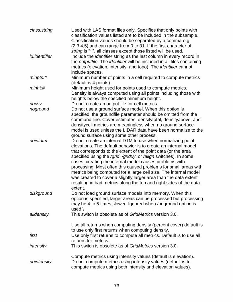
73


id:identifier Include the identifier string as the last column in every record in the outputfile. The identifier will be included in all files containing metrics (elevation, intensity, and topo). The identifier cannot include spaces.

minpts:# Minimum number of points in a cell required to compute metrics (default is 4 points).

minht:# Minimum height used for points used to compute metrics. Density is always computed using all points including those with heights below the specified minimum height.

nocsv Do not create an output file for cell metrics. noground Do not use a ground surface model. When this option is

specified, the groundfile parameter should be omitted from the command line. Cover estimates, densitytotal, densityabove, and densitycell metrics are meaningless when no ground surface model is used unless the LIDAR data have been normalize to the ground surface using some other process.

nointdtm Do not create an internal DTM to use when normalizing point elevations. The default behavior is to create an internal model that corresponds to the extent of the point data (or the area specified using the /grid, /gridxy, or /align switches). In some cases, creating the internal model causes problems with processing. Most often this caused problems for small areas with metrics being computed for a large cell size. The internal model was created to cover a slightly larger area than the data extent resulting in bad metrics along the top and right sides of the data extent.

diskground Do not load ground surface models into memory. When this option is specified, larger areas can be processed but processing may be 4 to 5 times slower. Ignored when /noground option is used.\

alldensity This switch is obsolete as of GridMetrics version 3.0. Use all returns when computing density (percent cover) default is to use only first returns when computing density.

first Use only first returns to compute all metrics. Default is to use all returns for metrics.

intensity This switch is obsolete as of GridMetrics version 3.0. Compute metrics using intensity values (default is elevation).

nointensity Do not compute metrics using intensity values (default is to compute metrics using both intensity and elevation values).

74

rgb:color Compute intensity metrics using the color value from the RGB color for the returns. Valid with LAS version 1.2 and newer data files that contain RGB information for each return (point record types 2 and 3). Valid color values are R, G, or B.

fuel Apply fuel parameter models (cannot be used with /first switch). grid:X,Y,W,H Force the origin of the output grid to be (X,Y) instead of

computing an origin from the data extents and force the grid to be W units wide and H units high...W and H will be rounded up to a multiple of cellsize.

gridxy:X1,Y1, X2,Y2




buffer:width Add an analysis buffer of the specified width (same units as LIDAR data) around the data extent when computing metrics but only output metrics for the area specified via /grid, /gridxy, or /align. When /buffer is used without one of these options, metrics are output for an area that is inside the actual extent of the return data as metrics within the buffer area are not output.

cellbuffer:width Add an analysis buffer specified as the number of extra rows and columns around the data extent when computing metrics but only output metrics for the area specified via /grid, /gridxy, or /align. When /cellbuffer is used without one of these options, metrics are output for an area that is inside the actual extent of the return data as metrics for the buffer area are not output.

strata:[#,#,#,…] Count returns in various height strata. # gives the upper limit for each strata. Returns are counted if their height is >= the lower limit and < the upper limit. The first strata contains points < the first limit. The last strata contains points >= the last limit. Default strata: 0.15, 1.37, 5, 10, 20, 30.

intstrata:[#,#,#,…] Compute metrics using the intensity values in various height strata. Strata for intensity metrics are defined in the same way as the /strata option. Default strata: 0.15, 1.37.

kde:[window,mult] Compute the number of modes and minimum and maximum node using a kernel density estimator. Window is the width of a moving average smoothing window in data units and mult is a multiplier for the bandwidth parameter of the KDE. Default window is 2.5 and the multiplier is 1.0

75

ascii Store raster files in ASCII raster format for direct import into ArcGIS. Using this option preserves metrics with negative values. Such values are lost when raster data are stored using the PLANS DTM format. This switch is ignored unless it is used with the /raster switch.

topo:dist,lat Compute topographic metrics using the groundfile(s) and output them in a separate file. Distance is the cell size for the 3 by 3 cell analysis area and lat is the latitude (+north, -south).

raster:layers It is likely that this option will be removed at some point. The amount of code required to implement this option is quite large and the DTM files produced by the option cannot support negative numbers. There are better ways to get individual metrics for input into other analyses. For example, you can use the CSV2Grid utility to extract specific columns from the .CSV files produced by GridMetrics. Use of the /raster option is discouraged. Create raster files containing the point cloud metrics. layers is a list of metric names separated by commas. Raster files are stored in PLANS DTM format or ASCII raster format when the /ascii switch is used. Topographic metrics are not available with the /raster:layers switch. Available metrics are:

count Number of returns above the minimum height

densitytotal total returns used for calculating cover densityabove returns above heightbreak densitycell Density of returns used for calculating

cover min minimum value for cell max maximum value for cell mean mean value for cell mode modal value for cell stddev standard deviation of cell values variance variance of cell values cv coefficient of variation for cell cover cover estimate for cell abovemean proportion of first (or all) returns above

the mean abovemode proportion of first (or all) returns above

the mode skewness skewness computed for cell kurtosis kurtosis computed for cell AAD average absolute deviation from mean

for the cell

76

p01 1st percentile value for cell (must be p01, not p1)

p05 5th percentile value for cell (must be p05, not p5)

p10 10th percentile value for cell p20 20th percentile value for cell p25 25th percentile value for cell p30 30th percentile value for cell p40 40th percentile value for cell p50 50th percentile value (median) for cell p60 60th percentile value for cell p70 70th percentile value for cell p75 75th percentile value for cell p80 80th percentile value for cell p90 90th percentile value for cell p95 95th percentile value for cell p99 99th percentile value for cell iq 75th percentile minus 25th percentile for

cell 90m10 90th percentile minus 10th percentile for

cell 95m05 95th percentile minus 5th percentile for

cell r1count Count of return 1 points above the

minimum height r2count Count of return 2 points above the








minimum height rothercount Count of other returns above the

minimum height allcover (all returns above cover ht) / (total

returns)

77

afcover (all returns above cover ht) / (total first returns)

allcount number of returns above cover ht allabovemean (all returns above mean ht) / (total

returns) allabovemode (all returns above ht mode) / (total

returns) afabovemean (all returns above mean ht) / (total first

returns) afabovemode (all returns above ht mode) / (total first

returns) fcountmean number of first returns above mean ht fcountmode number of first returns above ht mode allcountmean number of returns above mean ht allcountmode number of returns above ht mode totalfirst total number of 1st returns totalall total number of returns

For example, /raster:min,max,p75 would produce raster files containing the minimum, maximum and 75th percentile values for each cell.

Technical Details

Output from GridMetrics is divided into several files. The point cloud metrics are stored in two files. The first is identified as “elevation_stats” and the second as “intensity_stats”. The file with elevation metrics also contains a variety of cover metrics computed using combinations of first and all returns. If the /kde switch is used, its output variables (4 values) are placed at the end of all other metrics in the “elevation_stats” file. In addition, header files containing coordinate system and grid cell size information are created in the same folder as the metrics. The header files are used when data in CSV format are converted into ASCII raster format. When either the /strata or /intstrata options are used, their output is stored in a separate file (both elevation and intensity strata metrics in the same file). The file is identified as “strata_stats”. A header is also created that contains the coordinate systems and grid cell size information. When the /topo:dist,lat switch is used, a third set of output files containing topographic attributes is produced. For example, when /strata, /intstrata, and /topo switches are used and the outputfile is specified as “metrics.csv” the following output files are produced:

metrics_all_returns_elevation_stats.csv metrics_all_returns_elevation_stats_ascii_header.csv metrics_all_returns_intensity_stats.csv metrics_all_returns_intensity_stats_ascii_header.csv metrics_all_returns_strata_stats.csv metrics_all_returns_strata_stats_ascii_header.txt metrics_topo_stats.csv metrics_topo_stats_ascii_header.csv

78

If the /first switch is specified, the file names would change as follows:

metrics_first_returns_elevation_stats.csv metrics_first_returns_elevation_stats_ascii_header.csv metrics_first_returns_intensity_stats.csv metrics_first_returns_intensity_stats_ascii_header.csv metrics_first_returns_strata_stats.csv metrics_first_returns_strata_stats_ascii_header.txt metrics_topo_stats.csv metrics_topo_stats_ascii_header.csv

GridMetrics computes the following descriptive statistics:

Column Elevation metric Intensity metric

1 Row Row 2 Col Col 3 Center X Center X 4 Center Y Center Y 5 Total return count above htmin Total return count above htmin 6 Elev minimum Int minimum 7 Elev maximum Int maximum 8 Elev mean Int mean 9 Elev mode Int mode 10 Elev stddev Int stddev 11 Elev variance Int variance 12 Elev CV Int CV 13 Elev IQ Int IQ 14 Elev skewness Int skewness 15 Elev kurtosis Int kurtosis 16 Elev AAD Int AAD 17 Elev L1 Int L1 18 Elev L2 Int L2 19 Elev L3 Int L3 20 Elev L4 Int L4 21 Elev L CV Int L CV 22 Elev L skewness Int L skewness 23 Elev L kurtosis Int L kurtosis 24 Elev P01 Int P01 25 Elev P05 Int P05 26 Elev P10 Int P10 27 Elev P20 Int P20 28 Elev P25 Int P25 29 Elev P30 Int P30 30 Elev P40 Int P40 31 Elev P50 Int P50 32 Elev P60 Int P60 33 Elev P70 Int P70 34 Elev P75 Int P75 35 Elev P80 Int P80 36 Elev P90 Int P90 37 Elev P95 Int P95 38 Elev P99 Int P99

79

Column Elevation metric Intensity metric 39 Return 1 count above htmin 40 Return 2 count above htmin 41 Return 3 count above htmin 42 Return 4 count above htmin 43 Return 5 count above htmin 44 Return 6 count above htmin 45 Return 7 count above htmin 46 Return 8 count above htmin 47 Return 9 count above htmin 48 Other return count above htmin 49 Percentage first returns above

heightbreak

50 Percentage all returns above heightbreak

51 (All returns above heightbreak) / (Total first returns) * 100

52 First returns above heightbreak 53 All returns above heightbreak 54 Percentage first returns above

mean

55 Percentage first returns above mode

56 Percentage all returns above mean 57 Percentage all returns above mode 58 (All returns above mean) / (Total

first returns) * 100

59 (All returns above mode) / (Total first returns) * 100

60 First returns above mean 61 First returns above mode 62 All returns above mean 63 All returns above mode 64 Total first returns 65 Total all returns 66 Elev MAD median 67 Elev MAD mode 68 Canopy relief ratio

((mean - min) / (max – min))

69 Elev quadratic mean 70 Elev cubic mean 71 KDE elev modes 72 KDE elev min mode 73 KDE elev max mode 74 KDE elev mode range

When the /topo:dist,lat switch is used, the following metrics are computed:

Column Topographic metric

1 Row 2 Col 3 Center X 4 Center Y 5 Surface elevation 6 Surface slope (degrees)

80

Column Topographic metric 7 Surface aspect (degrees azimuth, 0

degrees at 12 o’clock, increasing clockwise)

8 Profile curvature * 100 (in direction of slope)

9 Plan curvature * 100 (perpendicular to slope)

10 Solar radiation index 11 Overall curvature

When the /strata or /intstrata switch is used, the computed metrics are stored in the same file. The first set of columns contains the elevation metrics and the second set of columns contains the intensity metrics. The bounding elevations for the elevation and intensity strata can be different so care should be taken to ensure that any additional analyses use the metric s correctly. The following strata metrics are computed:

Column Strata metric

1 Row

2 Col

3 Total return count for 1st strata

4 Minimum elevation for 1st strata

5 Maximum elevation for 1st strata

6 Average elevation for 1st strata

7 Mode of elevations for 1st strata

8 Median elevation for 1st strata

9 Standard deviation of elevations within the 1st strata

10 Coefficient of variation for elevations within the 1st strata

11 Skewness of elevations within the 1st strata

12 Kurtosis of elevations within the 1st strata

… Metrics for remaining elevation strata

Total return count for 1st strata

Minimum intensity for 1st strata

Maximum intensity for 1st strata

Average intensity for 1st strata

Mode of intensity for 1st strata

Median intensity for 1st strata

Standard deviation of intensity within the 1st strata

Coefficient of variation for intensity within the 1st strata

Skewness of intensity within the 1st strata

Kurtosis of intensity within the 1st strata

… Metrics for remaining intensity strata

The /raster switch is provided to make it easy to compute a few metrics and convert the layers into files compatible with ArcInfo. The PLANS DTM format used for the layers cannot represent negative values so you should be careful using this option as a few of the layers will often have negative values. In addition, the layers produced when the /raster switch is used must be held in memory so fewer points (returns) can be processed when the /raster switch is used. The actual effect on the number of points

81

depends on the number of raster layers requested and the size of the bare-ground surface models used to normalize return elevations. In general, use of the /raster switch is not recommended. You can easily extract specific metrics from the CSV output file to create ASCII raster files using the CSV2Grid utility and you can merge several ASCII raster files into a single file using the MergeRaster utility. When computing cover, returns with elevations <= heightbreak are counted. Cover values are computed as described in the CloudMetrics section. The specific equation is:

nstotalretur

kheightbreareturnsCover

#

To produce cover estimates that are meaningful, the cell size must be larger than individual tree crowns. With small cell sizes (less than 5 meters) the distribution of cover values over a large area tends to be heavy on values near 0 and 100 because each cell serves to test for the presence or absence of a tree instead of providing a reasonable sample area for assessing vegetation cover. For most forest types, cell sizes of 15-meters or larger produce good results. Figure 3 illustrates the concept of estimating canopy cover using LIDAR first return data. If the densitycell raster data layer is requested, it will specify the proportion of the returns above the cover height limit. Normally this would be the proportion of first returns. If the alldensitycell raster data layer is requested, the resulting layer would represent the proportion of all returns above the cover height limit. When the /grid, /gridxy, or /align switches are used, GridMetrics tests the extent of indexed LDA files and LAS files to see if any points in the file fall within the specified grid area. If the file extent and the grid area do not overlap, the file is skipped. This allows you to use GridMetrics to compute statistics for small sample areas without identifying the specific data tiles that contain the sample. You specify the desired sample area and all data tiles and let GridMetrics figure out which tiles contain points within the sample area. If you are not using indexed LDA files or LAS files, such an approach will result in slow performance as every point in all tiles must be read and tested to see if it is within the grid area. Distribution statistics (skewness and kurtosis) are computed using product moments and L moments as described in the CloudMetrics description. The median of the absolute deviations from the median (MADMedian) and the median of the absolute deviations from the mode (MADMode) are compute as described in the CloudMetrics description. The generalized mean for the 2nd power (also called the quadratic mean and labeled as “Elev quadratic mean”) and the 3rd power (labeled as “Elev cubic mean”) are computed as described in the CloudMetrics description.

82

When GridMetrics is used with the /topo:dist,lat switch, a solar radiation index (SRI) and other topographic indices are computed for each input point. SRI combines information about the aspect, slope, and latitude into a single index that describes the amount of solar radiation theoretically striking an arbitrarily oriented surface during the hour surrounding noon on the equinox (Keating et al. 2007). The parameters for the /topo switch define the size of the surface cell and the latitude for the study area. In operation, elevations are interpolated for points defining a three- by three-cell grid where each grid cell is dist by dist units. These elevations are then used to compute the slope, aspect, and curvature for the surface patch (Zevenbergen and Thorne 1987). For most applications, the distance (or cell size) should not be small. The overall goal is to describe the terrain shape and not to capture every micro-topographic detail. SRI as defined by Keating et al. (2007) ranges from -1.0 to 1.0 but the full range is not possible at every location due to the effect of latitude on the index. For GridMetrics, this range has been adjusted to range from 0.0 to 2.0. SRI does not consider the change in the amount of solar radiation that occurs over the course of a day or year or changes that result from topographic shading. However it distills information about slope, aspect, and latitude into a single linear value useful for comparing locations. When /topo:dist,lat is specified, output includes the slope, aspect, profile curvature (along the slope), plan curvature (across the slope), and SRI all reported with 6 decimal digits regardless of the storage type for the elevations in the surface model. The formula used to compute SRI (adapted from Keating et al. 2007) is:

aspectslopelatitudeslopelatitudeSRI cos*sin*sincos*cos0.1

where: latitude is the latitude in degrees with north latitudes positive and south latitudes

negative slope is the inclination of the surface from the horizontal position in degrees aspect is the surface azimuth angle in degrees relative to south (180.0 – calculated

aspect) The median, quartile and percentile values calculated for the points are computed using the following method (http://www.resacorp.com, last accessed December 2005):

83

The fuel models available in GridMetrics are taken from Andersen et al. (2005). The models are applicable to Douglas-fir forest types in Western Washington. Application to other forest types or geographic regions may produce questionable results. The specific parameters estimated are: canopy fuel weight, bulk density, base height, and height.

29025 6.1067.19.27.22)/( Dhhhakgweightfuelcanopy

037.1*)/(4.212.013.002.02.33.43 902510 Dhhhhcvemkgdensitybulkcanopy

Dhhhhmheightbasecanopy cv 8.88.10.27.03.192.3)( 755025

Dhhhhmheightcanopy 5.35.10.125.025.08.2)( 755025max

These models assume elevations are in meters and require that the bare-earth surface model be a good representation of the true ground surface. Multiple ground surface models can be used in GridMetrics to facilitate processing of large acquisitions. When using multiple ground surface models, the default behavior is to load only those models into memory that overlap the data extent or the extent specified using /grid, /gridxy, or /align (possibly in combination with the /buffer or /cellbuffer options). If you find that your computer has insufficient memory to process the desired area, you can try the /diskground option to use logic that does not read the ground surface models into memory. Use of the /diskground option will allow processing for larger areas but also slows the processing by a factor of 4 to 5. To maximize processing speed, it is best to reduce the extent of the area processed rather than use the /diskground option. When using the /RGB option, you can only specific a single color component. This means that to compute metrics using the Red, Green, and Blue components requires three separate runs of GridMetrics. Output from the color metrics will be stored in separate files labeled to identify the color component used to compute the metrics.

Examples

The following command will compute metrics using elevations values and store them in CSV format. Cover values are computed using a height break of 3 meters and the metrics are computed for a 15- by 15-meter grid.

GridMetrics 000263_ground_1m.dtm 3 15 000263_metrics.csv 000263.las

The following command will compute metrics using elevations values and store them in CSV format. Metrics will cover a 1000 by 1000 meter area. The analysis area is buffered by 100 meters on all sides but the output metrics will only cover the extent specified in the /gridxy option. The ground model specification is expanded into a list containing several ground models. However, only the ground surface models that

84

overlap the buffered analysis area are loaded and used for processing. Cover values are computed using a height break of 3 meters and the metrics are computed for a 15- by 15-meter grid.

GridMetrics /gridxy:634000,7546000,635000,7547000 /buffer:100 *.dtm 3 15

Tile38_metrics.csv *.las

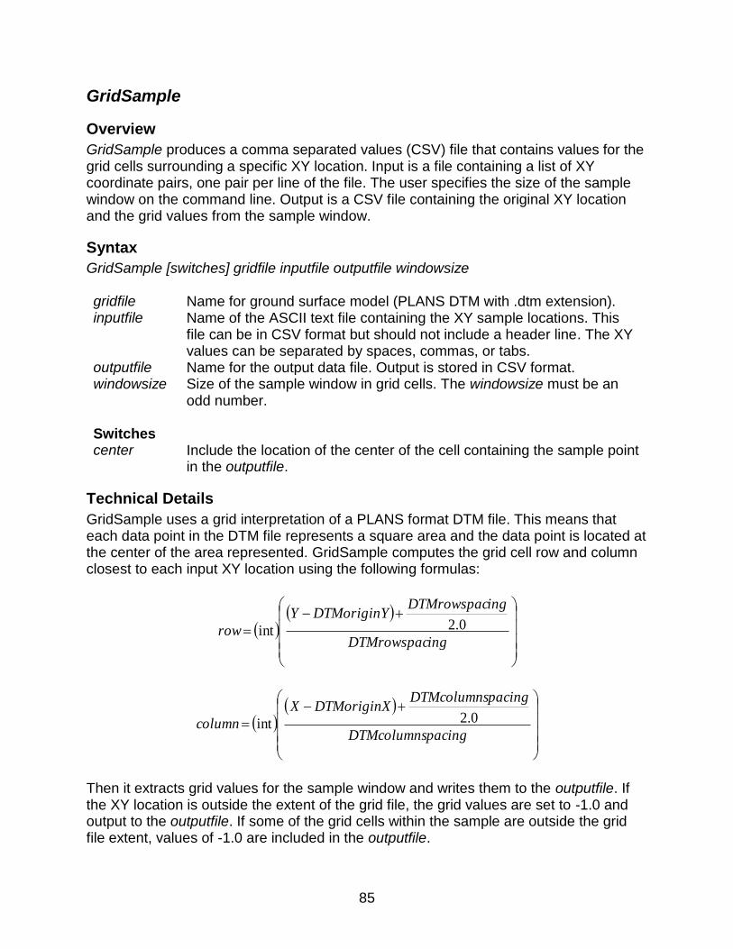
85

GridSample

Overview

GridSample produces a comma separated values (CSV) file that contains values for the grid cells surrounding a specific XY location. Input is a file containing a list of XY coordinate pairs, one pair per line of the file. The user specifies the size of the sample window on the command line. Output is a CSV file containing the original XY location and the grid values from the sample window.

Syntax

GridSample [switches] gridfile inputfile outputfile windowsize gridfile Name for ground surface model (PLANS DTM with .dtm extension). inputfile Name of the ASCII text file containing the XY sample locations. This

file can be in CSV format but should not include a header line. The XY values can be separated by spaces, commas, or tabs.

outputfile Name for the output data file. Output is stored in CSV format. windowsize Size of the sample window in grid cells. The windowsize must be an

odd number. Switches

center Include the location of the center of the cell containing the sample point in the outputfile.

Technical Details

GridSample uses a grid interpretation of a PLANS format DTM file. This means that each data point in the DTM file represents a square area and the data point is located at the center of the area represented. GridSample computes the grid cell row and column closest to each input XY location using the following formulas:

ingDTMrowspac

ingDTMrowspacDTMoriginYY

row 0.2int

pacingDTMcolumns

pacingDTMcolumnsDTMoriginXX

column 0.2int

Then it extracts grid values for the sample window and writes them to the outputfile. If the XY location is outside the extent of the grid file, the grid values are set to -1.0 and output to the outputfile. If some of the grid cells within the sample are outside the grid file extent, values of -1.0 are included in the outputfile.

86

Grid values are output by rows starting at the upper left corner of the sample area. Column labels are provided in the outputfile to indicate the arrangement of sample values. All samples associated with a location are output on a single line within the CSV file. Users that want to use the CSV files with Excel should be aware that there are limits on the number of columns that can be read from CSV files. This limit varies depending on the Excel version. The output CSV file reports grid values with 6 decimal digits for grid files that contain floating point values and with 0 decimal digits for grid files that contain integer values.

Examples

The following example reads locations from the file named plotsSE.txt and outputs grid values in a 5 by 5 pixel window from the grid surface canopy_complexity.dtm into the outputfile named plot_samples.csv.

GridSample canopy_complexity.dtm plotsSE.txt plot_sample.csv 5

The inputfile, plotsSE.txt contains the following records:

524750.0,5200000.0

524750.0,5200250.0

524750.0,5200500.0

524750.0,5200750.0

524750.0,5201000.0

525000.0,5200000.0

525000.0,5200250.0

525000.0,5200500.0

525000.0,5200750.0

525000.0,5201000.0

The outputfile, plot_samples.csv contains the following values (values were truncated to one decimal place for this example):

X,Y,"R+1 C-1","R+1 C+0","R+1 C+1","R+0 C-1","R+0 C+0","R+0 C+1","R-1 C-1","R-1 C+0","R-1 C+1"

524750.0,5200000.0,156.2,156.6,156.7,156.7,156.9,157.1,156.8,157.0,157.2

524750.0,5200250.0,162.5,162.2,161.7,162.6,162.4,161.8,162.4,162.5,162.0

524750.0,5200500.0,-1.0,-1.0,-1.0,-1.0,-1.0,-1.0,-1.0,-1.0,-1.0

524750.0,5200750.0,-1.0,-1.0,-1.0,-1.0,-1.0,-1.0,-1.0,-1.0,-1.0

524750.0,5201000.0,-1.0,-1.0,-1.0,-1.0,-1.0,-1.0,-1.0,-1.0,-1.0

525000.0,5200000.0,146.9,147.0,146.9,146.8,147.0,147.0,147.1,147.1,146.7

525000.0,5200250.0,143.9,143.6,143.3,144.0,143.8,143.5,144.3,144.0,143.7

525000.0,5200500.0,-1.0,-1.0,-1.0,-1.0,-1.0,-1.0,-1.0,-1.0,-1.0

525000.0,5200750.0,-1.0,-1.0,-1.0,-1.0,-1.0,-1.0,-1.0,-1.0,-1.0

525000.0,5201000.0,-1.0,-1.0,-1.0,-1.0,-1.0,-1.0,-1.0,-1.0,-1.0

87

GridSurfaceCreate

Overview

GridSurfaceCreate creates a gridded surface model using collections of random points. The surface model is stored in PLANS DTM format using floating point elevation values. Individual cell elevations are calculated using the average elevation of all points within the cell. GridSurfaceCreate is most often used with bare-earth point sets obtained from LIDAR vendors or by using the GroundFilter program.

Syntax

GridSurfaceCreate [switches] surfacefile cellsize xyunits zunits coordsys zone horizdatum vertdatum datafile1 datafile2... surfacefile Name for output surface file (stored in PLANS DTM format with .dtm

extension). cellsize Grid cell size for the surface. xyunits Units for LIDAR data XY:



coordsys Coordinate system for the surface: 0 for unknown, 1 for UTM, 2 for state plane.

zone Coordinate system zone for the surface (0 for unknown). horizdatum Horizontal datum for the surface:


vertdatum Vertical datum for the surface: 0 for unknown, 1 for NGVD29, 2 for NAVD88, 3 for GRS80.



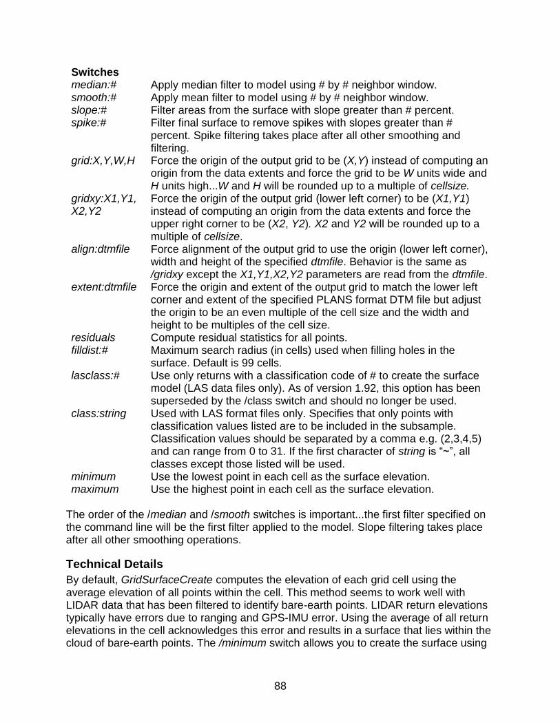
88

Switches median:# Apply median filter to model using # by # neighbor window. smooth:# Apply mean filter to model using # by # neighbor window. slope:# Filter areas from the surface with slope greater than # percent. spike:# Filter final surface to remove spikes with slopes greater than #

percent. Spike filtering takes place after all other smoothing and filtering.


gridxy:X1,Y1, X2,Y2




residuals Compute residual statistics for all points. filldist:# Maximum search radius (in cells) used when filling holes in the

surface. Default is 99 cells. lasclass:# Use only returns with a classification code of # to create the surface

model (LAS data files only). As of version 1.92, this option has been superseded by the /class switch and should no longer be used.


minimum Use the lowest point in each cell as the surface elevation. maximum Use the highest point in each cell as the surface elevation.

The order of the /median and /smooth switches is important...the first filter specified on the command line will be the first filter applied to the model. Slope filtering takes place after all other smoothing operations.

Technical Details

By default, GridSurfaceCreate computes the elevation of each grid cell using the average elevation of all points within the cell. This method seems to work well with LIDAR data that has been filtered to identify bare-earth points. LIDAR return elevations typically have errors due to ranging and GPS-IMU error. Using the average of all return elevations in the cell acknowledges this error and results in a surface that lies within the cloud of bare-earth points. The /minimum switch allows you to create the surface using

89

the lowest point in each cell as the surface elevation. For some applications, this results in surfaces that are better behaved that those using the average of all return elevations in the cell. However, when using the /minimum switch you should specify a small cell size to avoid producing a surface that lies below the bare-earth point set. In general, you need to experiment with settings for GroundFilter and GridSurfaceCreate to find the combination of options that produce bare-earth surfaces that meet your needs. In general, smoothing using the /median or /smooth switches is unnecessary provided that the data points used to create the surface are truly bare-earth points. Smoothing will result in some loss of surface detail particularly in areas with sharply defined features such as road cut banks, stream banks, and eroded areas. For data point sets that included some residual returns from vegetation, smoothing (especially using the /median switch) may be necessary to produce a useable ground surface. For data sets acquired over urban areas, it is not uncommon to have returns from building rooftops included in the bare-earth point set. For such data, smoothing with a window size that is larger than the largest building footprint is required to remove the surface anomalies associated with the returns from rooftops. Such smoothing generally degrades the terrain features to a point where most surface detail is lost. Filtering to remove steep spikes, specified using the /spike switch, works well to remove spikes related to residual returns from vegetation in areas of moderate topography. Spikes are only removed if they are also a local maximum within a 3 by 3 point window. In areas with steep topography, spike filtering may result in excessive smoothing of terrain features; especially those features that define transitions from low slope to high slop areas. Cells that contain no points are filled by interpolation using neighboring cells. Cells on the edge of the data coverage with no neighbors with valid elevations in one or more directions are flagged with NODATA values.

Examples

The following command produces a surface model using a 1- by 1-meter grid. No smoothing is done for the final surface. Data are in the UTM coordinate system, zone 10, with units for both horizontal values and elevations of meters. The data uses the NAD83 horizontal and NAVD88 vertical datums.

GridSurfaceCreate 000263_gnd_1m.dtm 1 m m 1 10 2 2 000263_gnd_pts.lda

The following command produces a surface model using a 1- by 1-meter grid. A median smoothing filter using a 3 by 3 cell window is used to smooth the final surface.

GridSurfaceCreate /median:3 000263_gnd_1m.dtm 1 m m 1 10 2 2 000263_gnd_pts.lda

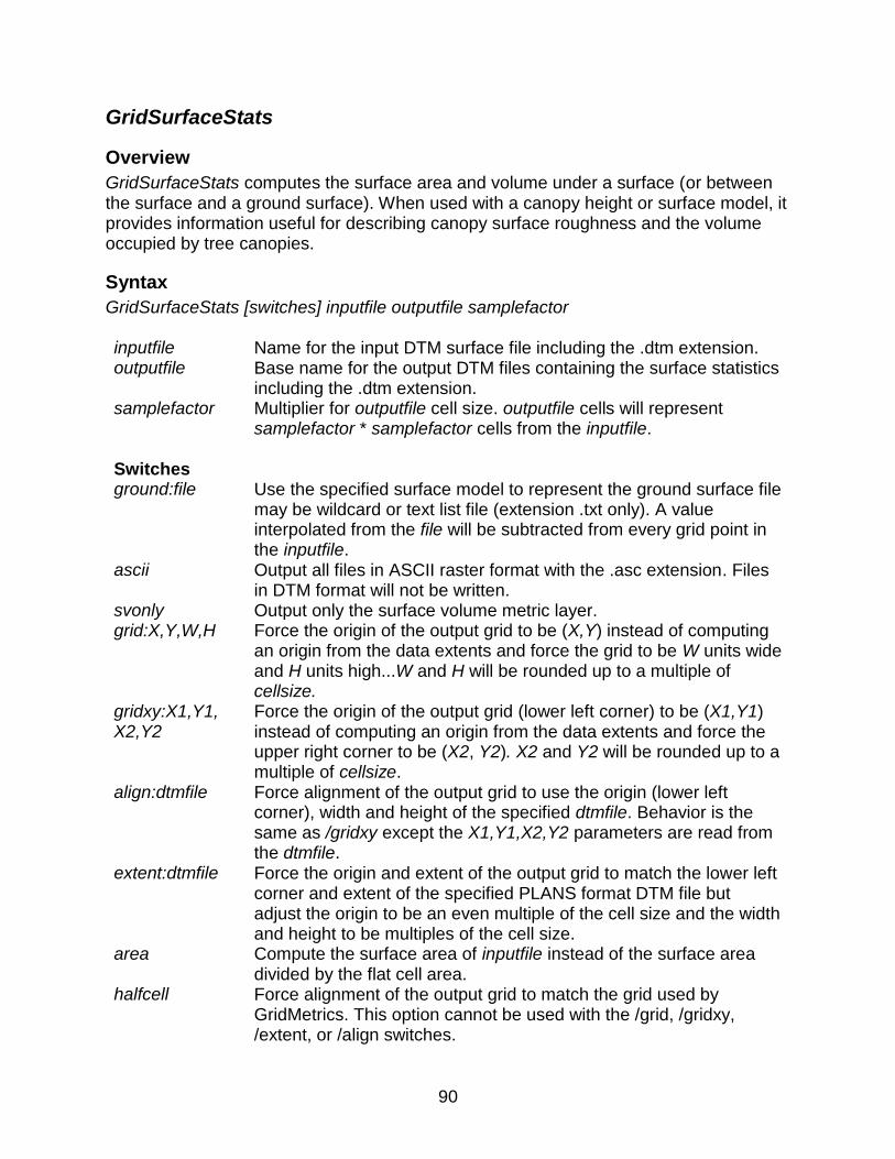
90

GridSurfaceStats

Overview

GridSurfaceStats computes the surface area and volume under a surface (or between the surface and a ground surface). When used with a canopy height or surface model, it provides information useful for describing canopy surface roughness and the volume occupied by tree canopies.

Syntax

GridSurfaceStats [switches] inputfile outputfile samplefactor inputfile Name for the input DTM surface file including the .dtm extension. outputfile Base name for the output DTM files containing the surface statistics

including the .dtm extension. samplefactor Multiplier for outputfile cell size. outputfile cells will represent

samplefactor * samplefactor cells from the inputfile. Switches

ground:file Use the specified surface model to represent the ground surface file may be wildcard or text list file (extension .txt only). A value interpolated from the file will be subtracted from every grid point in the inputfile.

ascii Output all files in ASCII raster format with the .asc extension. Files in DTM format will not be written.

svonly Output only the surface volume metric layer. grid:X,Y,W,H Force the origin of the output grid to be (X,Y) instead of computing

an origin from the data extents and force the grid to be W units wide and H units high...W and H will be rounded up to a multiple of cellsize.

gridxy:X1,Y1, X2,Y2




area Compute the surface area of inputfile instead of the surface area divided by the flat cell area.

halfcell Force alignment of the output grid to match the grid used by GridMetrics. This option cannot be used with the /grid, /gridxy, /extent, or /align switches.

91

Technical Details

Surface area and volume are computed by dividing each grid cell in the surface into two triangles from the lower left to the upper right corner. Then the area of each triangle is computed using the 3D coordinates of the triangle vertices. Area is the magnitude of the cross product of the three vertices. Volume under the surface for each triangle is computed by multiplying the flat triangle area (1/2 of the grid cell area) by the average elevation (or height) of the three vertices. Totals for each cell in the outputfile are computed by summing the areas and volumes for the samplefactor * samplefactor cells from the inputfile. Area and volume are only computed when all four corners of a cell in the inputfile have valid data. If any vertex has an invalid elevation (or height), the area and volume for the entire cell is 0.0. The /grid, /gridxy, /align, and /extent switches allow you to force the extent of the surface metrics to provide better alignment with output from GridMetrics.

92

GridSurfaceStats computes the following values for each samplefactor * samplefactor cell area from the input surface:

Value Description Maximum height Maximum height value for the samplefactor *

samplefactor cell window in the input surface Potential volume Volume under the samplefactor * samplefactor cell

window using the maximum height. Surface area ratio 𝑆𝑢𝑟𝑓𝑎𝑐𝑒 𝑎𝑟𝑒𝑎 𝑜𝑓 𝑠𝑎𝑚𝑝𝑙𝑒𝑓𝑎𝑐𝑡𝑜𝑟 ∗ 𝑠𝑎𝑚𝑝𝑙𝑒𝑓𝑎𝑐𝑡𝑜𝑟 𝑐𝑒𝑙𝑙

𝐹𝑙𝑎𝑡 𝑎𝑟𝑒𝑎 𝑜𝑓 𝑡ℎ𝑒 𝑠𝑎𝑚𝑝𝑙𝑒𝑓𝑎𝑐𝑡𝑜𝑟 ∗ 𝑠𝑎𝑚𝑝𝑙𝑒𝑓𝑎𝑐𝑡𝑜𝑟 𝑐𝑒𝑙𝑙

Surface area (with /area switch)

Surface area of samplefactor * samplefactor cell

Surface volume Volume under the samplefactor * samplefactor cell window using the cell heights.

Surface volume ratio 𝑆𝑢𝑟𝑓𝑎𝑐𝑒 𝑣𝑜𝑙𝑢𝑚𝑒

𝑃𝑜𝑡𝑒𝑛𝑡𝑖𝑎𝑙 𝑣𝑜𝑙𝑢𝑚𝑒

Examples

The following example computes area and volume for the canopy height model named ALLAREA_CHM.DTM using a 5 by 5 window and writes the results to files whose names use the base name: CHM_STATS.DTM:

GridSurfaceStats ALLAREA_CHM.DTM CHM_STATS.DTM 5

Five output files are produced with names formed by adding the following to the base outputfile name:

_max_height _potential_volume _surface_area_ratio _surface_volume _surface_volume_ratio

In the example above the following files would be created:

CHM_STATS _max_height.dtm CHM_STATS _potential_volume.dtm CHM_STATS _surface_area_ratio.dtm CHM_STATS _surface_volume.dtm CHM_STATS _surface_volume_ratio.dtm

93

GroundFilter

Overview

GroundFilter is designed to filter a cloud of LIDAR returns to identify those returns that lie on the probable ground surface (bare-earth points). GroundFilter does not produce a perfect set of bare-earth returns in that it does not completely remove returns from large, relatively flat, elevated surface such as building roofs. Most vegetation returns are removed with the appropriate coefficients for the weight function and sufficient iterations. Experimentation with GroundFilter has shown that the default coefficients for the weight function produce good results in high-density point clouds (> 4 returns/sq m). The program can be used with low-density point clouds but some experimentation may be needed to select appropriate coefficients. In general, GroundFilter produces point sets that result in surface models that are adequate for calculating vegetation heights. The point set and resulting models may not be adequate when the bare-earth surface is the primary product. The output from GroundFilter is a file containing only the points classified as ground returns stored in LDA format. The output file can be used with the GridSurfaceCreate or TINSurfaceCreate utilities to produce a ground surface model.

Syntax

GroundFilter [switches] outputfile cellsize datafile1 datafile2 ...

outputfile The name of the output LIDAR data file containing points classified as bare-earth returns.

cellsize The cell size used for intermediate surface models. This is used for intermediate surfaces and is not the cell size for the final ground surface model created using GridSurfaceCreate or TINSurfaceCreate.



Switches

surface Create a surface model using the final ground points.

median:# Use a median filter for the intermediate surface model with # by # window.

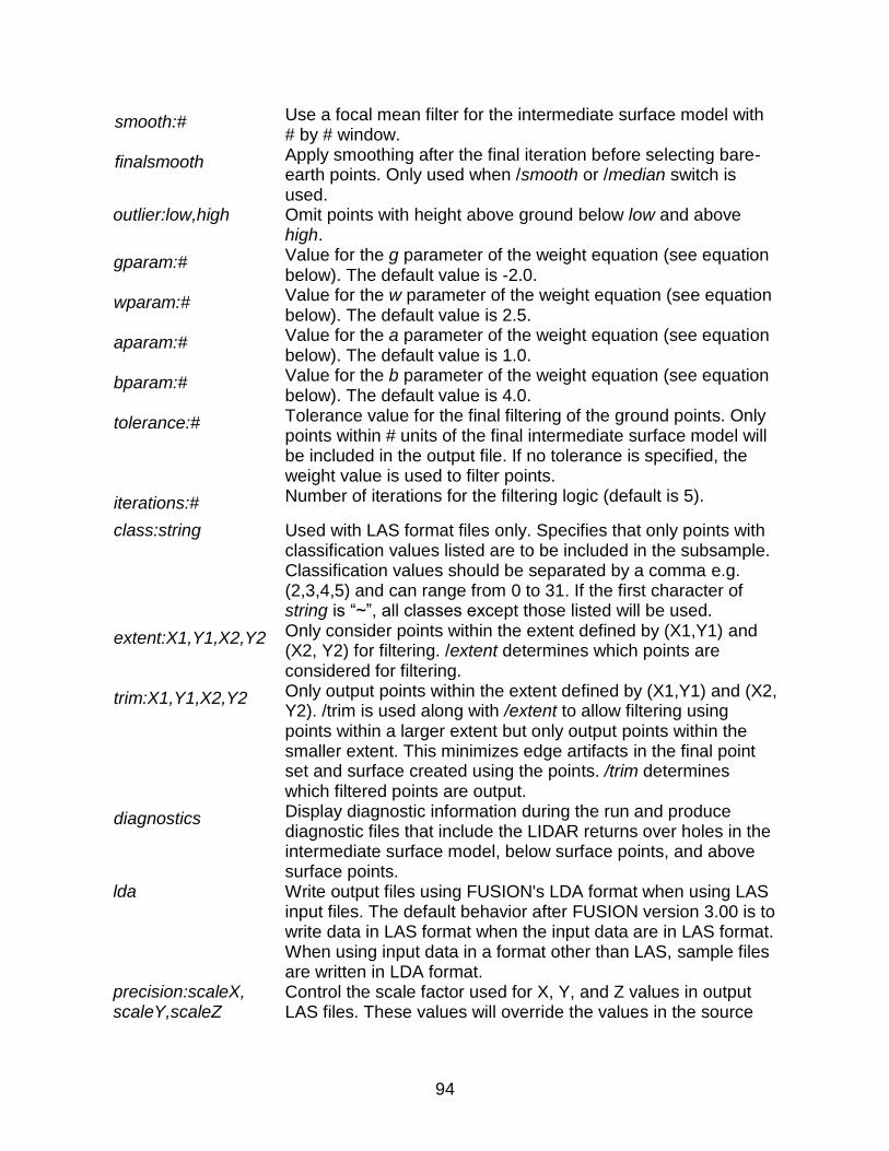
94

smooth:# Use a focal mean filter for the intermediate surface model with # by # window.

finalsmooth Apply smoothing after the final iteration before selecting bare-earth points. Only used when /smooth or /median switch is used.

outlier:low,high Omit points with height above ground below low and above high.

gparam:# Value for the g parameter of the weight equation (see equation below). The default value is -2.0.

wparam:# Value for the w parameter of the weight equation (see equation below). The default value is 2.5.

aparam:# Value for the a parameter of the weight equation (see equation below). The default value is 1.0.

bparam:# Value for the b parameter of the weight equation (see equation below). The default value is 4.0.

tolerance:# Tolerance value for the final filtering of the ground points. Only points within # units of the final intermediate surface model will be included in the output file. If no tolerance is specified, the weight value is used to filter points.

iterations:# Number of iterations for the filtering logic (default is 5).


extent:X1,Y1,X2,Y2 Only consider points within the extent defined by (X1,Y1) and (X2, Y2) for filtering. /extent determines which points are considered for filtering.

trim:X1,Y1,X2,Y2 Only output points within the extent defined by (X1,Y1) and (X2, Y2). /trim is used along with /extent to allow filtering using points within a larger extent but only output points within the smaller extent. This minimizes edge artifacts in the final point set and surface created using the points. /trim determines which filtered points are output.

diagnostics Display diagnostic information during the run and produce diagnostic files that include the LIDAR returns over holes in the intermediate surface model, below surface points, and above surface points.



Control the scale factor used for X, Y, and Z values in output LAS files. These values will override the values in the source

95

LAS files. There is rarely any need for the scale parameters to be smaller than 0.001.

The order of the /median and /smooth switches is important...the first filter specified on the command line will be the first filter applied to the model. Slope filtering takes place after all other smoothing operations. The /extent and /trim options allow you to filter data for specific areas with a project or to overlay a processing grid over large datasets. When filtering large datasets, you can manually generate a processing tile arrangement and then specify the corner coordinates of each tile using the /trim option. Add a buffer to the corner coordinates and use the buffered coordinates with the /extent option. This should provide a set of filtered ground points that will produce surface models with minimal edge artifacts. If you are processing data using scripts generated by LTKProcessor or AreaProcessor, use the buffered tile coordinates with the /extent option and the unbuffered coordinates with the /trim option in the batch file used to process each tile.

Technical Details

The filtering algorithm (adapted from Kraus and Pfeifer, 1998) is based on linear prediction (Kraus and Mikhail, 1972) with an individual accuracy for each measurement. It is implemented as an iterative process. In the first step, a surface is computed with equal weights for all LIDAR points. This results in a surface that lies between the true ground and the canopy surface. Terrain points are more likely to be below the surface and vegetation points above the surface. The distance and direction to the surface is used to compute weights for each LIDAR point using the following weight function:

The parameters a and b determine the steepness of the weight function. For most applications values of 1.0 and 4.0 for a and b respectively have produced adequate results. The shift value, g, determines which points are assigned a weight of 1.0 (the maximum weight value). Points below the surface by more than g, are assigned a weight of 1.0. The above ground offset parameter, w, is used to establish an upper limit for points to have an influence on the intermediate surface. Points above the level defined by (g + w) are assigned a weight of 0.0. In the current implementation, values for g and w are fixed throughout the filtering run. Kraus and Pfeifer, 1998 used an adaptive process to modify the g parameter for each iteration. After the final iteration, bare-earth points are selected using the final intermediate surface. All points with elevations that satisfy the first two conditions of the weight function are considered bare-earth points. If the /tolerance:# switch is used, all points within the specified tolerance of the final surface are considered bare-earth points.

96

The /finalsmooth switch will result in slightly more aggressive smoothing of the intermediate surface model just before the final point selection process. In general, the additional smoothing results in a bare-earth point set that does not include points along sharply defined features such as road cut banks, stream banks, and eroded areas. Users should experiment with this switch to see if it meets their needs. When the /surface switch is used, a surface model is created using the final bare-earth points. The cell elevation is the average elevation of all points in a cell. The model cell size is the same as the intermediate surface cell size (specified by cellsize and smoothing is done depending on the /smooth and /median switches. In general, the surface model produced by GroundFilter is too coarse to be useful. It provides a quick check on the results of the bare-earth filtering as the resulting PLANS DTM file can be displayed for evaluation in the PDQ viewer. Diagnostics, enabled using the /diagnostics switch, can help diagnose situations where GroundFilter does not seem to be producing good bare-earth point sets. Diagnostics include descriptive summaries for each iteration and the intermediate surface models produced for each iteration. In addition, the PDQ viewer will be launched to show each intermediate surface as it is created.

Examples

The following command filters a data file and produces a new data file that contains only bare-earth points:

GroundFilter 000263_ground_pts.lda 5 000263.las

The following command uses 8 iterations, a g value of 0.0, and a w value of 0.5 to filter a data file and produces a new data file that contains only bare-earth points:

GroundFilter /gparam:0 /wparam:0.5 /iterations:8 000263_ground_pts.lda 5 000263.las

97

ImageCreate

Overview

ImageCreate creates an image from LIDAR data using the intensity value or elevation of the highest return within an image pixel. Optionally uses the height above a surface model to create the image. The output image is geo-referenced using a world file. The extent of the image is computed so that the image origin is a multiple of the pixel size. The default image file format is JPEG.

Syntax

ImageCreate [switches] ImageFileName PixelSize DataFile1 DataFile2 ... DataFileN

ImageFileName Name for the output image file. The file will be stored in the specified format regardless of the extension.

PixelSize Size (in the same units as the LIDAR data) of each pixel in the output image.

DataFile1…DataFileN LIDAR data files stored in binary LDA or LAS formats or ASCII LIDARDAT format (LIDARDAT format may not be supported in future versions).

Switches

bmp Store the output image file in Windows BMP format and set output image file extension to “.bmp”.

jpeg Store the output image file in JPEG format and set output image file extension to “.jpg”.

coloroption:n Method used to assign color to each image pixel. Valid values for n and their interpretation are: 0 Assign color using intensity 1 Assign color using elevation 2 Assign color using height above surface.

dtm:filename Name of the surface file used to compute heights. Only PLANS format surface models are recognized.

minimum:value Minimum value used to constrain the color assigned to a pixel. Returns with values less than value will be colored using the starting color.

maximum:value Maximum value used to constrain the color assigned to a pixel. Returns with values greater than value will be colored using the ending color.

startcolor:value Starting color in the color ramp used to assign pixel colors. Value can be a single number representing a combined RGB color or a series of three values separated by commas representing the R, G, and B color components.

stopcolor:value Ending color in the color ramp used to assign pixel colors. Value can be a single number representing a combined RGB color or a series of three values separated by commas representing the R, G, and B color components.

98

hsv Use the HSV color model to create the color ramp. rgb Use the RGB color model to create the color ramp. backgroundcolor:value Background color for areas of the image not covered by

LIDAR data. Value can be a single number representing a combined RGB color or a series of three values separated by commas representing the R, G, and B color components.

Technical Details

When creating an image using intensity values for individual LIDAR returns, ImageCreate automatically scales the range of values from 0.0 to the intensity value corresponding to the 95th percentile of intensity values in the data. You can override this behavior by specifying a minimum and maximum range value. Image extents are computed after scanning the LIDAR data for minimum and maximum XY values. The min/max values are adjusted so the area covered by the image always begins on an even multiple of the cell size. To make the adjustments, the area covered by the image is expanded and shifted to the correct origin. ImageCreate creates images using the JPEG format by default. The /bmp switch allows creation of images in windows BMP format. The extension of the ImageFileName will be changed depending on the image format. This means that the image created by ImageCreate may have a name different from that specified by ImageFileName if you specify the wrong extension for the image file format being produced.

Examples

The following example creates an image using the intensity values stored in tile001.lda. The range of intensity values is truncated using a minimum value of 10 and a maximum value of 90 and the image uses pixels that are 2- by 2-meters.

ImageCreate /rgb /min:10 /max:90 /back:0,0,0 tile001_intensity.bmp 2 tile001.lda

99

IntensityImage

Overview

Airborne laser scanning (commonly referred to as LIDAR) data have proven to be a good source of information for describing the ground surface and characterizing the size and extent of man-made features such as road systems and buildings. The technology has gained a strong foothold in mapping operations traditionally dominated by photogrammetric techniques. In the forestry context, airborne laser scanning data have been used to produce detailed bare-earth surface models and to characterize vegetation structure and spatial extent. Hyyppä et al. (2004) provide an overview of LIDAR applications for forest measurements. One often overlooked component of LIDAR data, return intensity, is seldom used in analysis procedures. LIDAR return intensity is related to the ratio of the amount of the laser energy detected by the receiver for a given reflection point to the amount of total energy emitted for the laser pulse (Baltsavias, 1999; Wehr and Lohr, 1999). Because this ratio is quite small (Baltsavias, 1999), intensity values reported in LIDAR data are scaled to a more useful range (8-bit values are common). Intensity values are collected by most sensors in use today and providers include the intensity values in point cloud data files stored in the standard LAS format (ASPRS, 2005). Flood (2001) points out that while intensity data have been available for some time, their use in commercial data processing workflows is limited. Song et al. (2002) evaluated the potential for identifying a variety of surface materials (asphalt, grass, house roof, and trees) using LIDAR intensity in an urban environment. Charaniya et al. (2004) used LIDAR point data, LIDAR intensity, USGS 10m-resolution digital elevation model, and black-and-white ortho-photographs to classify LIDAR points into the same categories. Hasegawa (2006) conducted experiments to investigate the effects of target material, scan geometry and distance-to-target on intensity values using a typical airborne scanner attached to a fixed mount on the ground. He also evaluated the use of airborne LIDAR data to identify a variety of materials. He concluded that some materials were easily separated (soil, gravel, old asphalt, and grass) while others were not easy to separate (cement, slate, zinc, brick, and trees). Brennan and Webster (2006) utilized a rule-based object-oriented approach to classify a variety of land cover types using LIDAR height and intensity data. They found that both height and intensity information were needed to separate and classify ten land cover types. Brandtberg (2007) also found that use of intensity data significantly improved LIDAR detection and classification of leaf-off eastern deciduous forests.

Syntax

IntensityImage [switches] CellSize ImageFile DataFile1 DataFile2 CellSize The pixel size used for the intensity image (same units as LIDAR

data). ImageFile Name for the image file. datafile1 First LIDAR data file (LDA, LAS, ASCII LIDARDAT formats)...may be

wildcard or name of text file listing the data files. If wildcard or text file is used, no other datafile# parameters will be recognized.

100


Switches

minint:# Minimum intensity percentile used for the image. Default is 2 percent.

maxint:# Maximum intensity percentile used for the image. Default is 98 percent.

intrange:min,max

Force the scaling of intensity values using the specified min and max values. Setting the min value to -1 should force the output range to start with 1 instead of 0. Doing this in combination with /void:0,0,0 will allow you to identify areas with no data in the output image as they will have a value of 0 for all color bands.

intcell:# Cell size multiplier for intermediate images. Default is 1.5. void:R,G,B Color for areas with no data values. Default is red (255, 0, 0). allreturns Use all returns to create the intensity image instead of only first

returns. lowest Use the lowest return in the pixel area to assign the intensity value.

The /lowest switch should be used with the /allreturns switch for best effect.

lowall Combines the /lowest and /allreturns switches. /lowall will have no effect when used with either the /lowest or /allreturns switches.

saveint Save the intermediate image files. Usually used to diagnose problems.

rasterorigin Force alignment to match other raster products generated from point data (offsets the origin of the image by 1/2 pixel).

diskonly Do not attempt to read all returns into memory for processing. hist Produce the intensity histogram data files. Histogram data files are

produced in CSV format for both the raw frequency histogram and the normalized cumulative frequency histogram.

jpg Save the intensity image using the JPEG format. The default format is BMP.

projection:filename

Associate the specified projection file with image products.


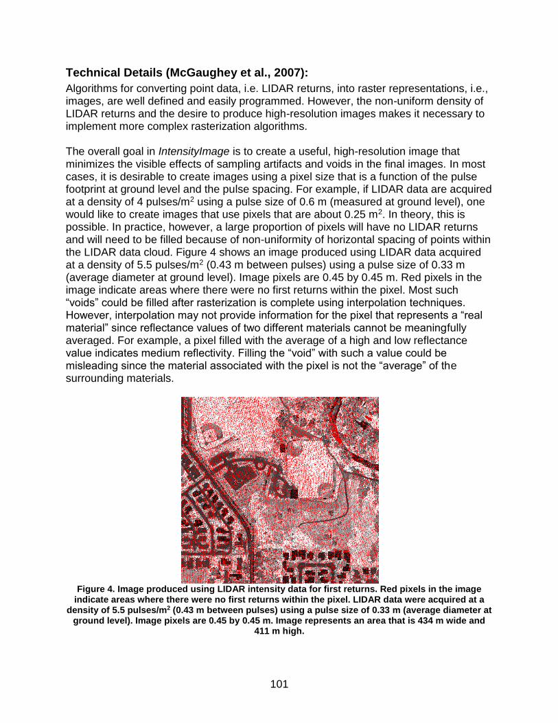
101

Technical Details (McGaughey et al., 2007):

Algorithms for converting point data, i.e. LIDAR returns, into raster representations, i.e., images, are well defined and easily programmed. However, the non-uniform density of LIDAR returns and the desire to produce high-resolution images makes it necessary to implement more complex rasterization algorithms. The overall goal in IntensityImage is to create a useful, high-resolution image that minimizes the visible effects of sampling artifacts and voids in the final images. In most cases, it is desirable to create images using a pixel size that is a function of the pulse footprint at ground level and the pulse spacing. For example, if LIDAR data are acquired at a density of 4 pulses/m2 using a pulse size of 0.6 m (measured at ground level), one would like to create images that use pixels that are about 0.25 m2. In theory, this is possible. In practice, however, a large proportion of pixels will have no LIDAR returns and will need to be filled because of non-uniformity of horizontal spacing of points within the LIDAR data cloud. Figure 4 shows an image produced using LIDAR data acquired at a density of 5.5 pulses/m2 (0.43 m between pulses) using a pulse size of 0.33 m (average diameter at ground level). Image pixels are 0.45 by 0.45 m. Red pixels in the image indicate areas where there were no first returns within the pixel. Most such “voids” could be filled after rasterization is complete using interpolation techniques. However, interpolation may not provide information for the pixel that represents a “real material” since reflectance values of two different materials cannot be meaningfully averaged. For example, a pixel filled with the average of a high and low reflectance value indicates medium reflectivity. Filling the “void” with such a value could be misleading since the material associated with the pixel is not the “average” of the surrounding materials.

Figure 4. Image produced using LIDAR intensity data for first returns. Red pixels in the image

indicate areas where there were no first returns within the pixel. LIDAR data were acquired at a density of 5.5 pulses/m2 (0.43 m between pulses) using a pulse size of 0.33 m (average diameter at

ground level). Image pixels are 0.45 by 0.45 m. Image represents an area that is 434 m wide and 411 m high.

102

To help fill void areas and produce high resolution images, we have implemented an algorithm similar to full-scene anti-aliasing algorithms common in computer graphics (Woo et al., 1997). The basic approach is to render the point data (convert from points to a raster image) several times using a slightly offset, or “jittered”, raster origin. Our implementation uses eight iterations using origin offsets shown in Table 2 and Figure 5. The offsets are multiplied by the raster cell size. In Figure 5, the black diamond in the center of the gray “cell” is the origin for the final image. The final image is produced by sampling the eight images at a location that corresponds to the center of the final image pixels. The grayscale intensity for the final image is computed as the average of the valid values (non-void) from the eight images. To help eliminate void pixels, we create the images for the iterations using a slightly larger pixel size, 1.5 times the final pixel size, and then create the final image using the user-specified pixel size. Final images include geo-referencing information stored in a world file. Figure 6 shows the final composite image produced from the same data used for the intermediate image shown in Figure 4. Notice that most of the void areas have been eliminated. The remaining large, red areas are open water (swimming pools, river) and a glass-covered atrium in the building in the lower-left corner of the image. For most applications, the remaining void pixels do not detract from the overall appearance and utility of the image.

Table 2. Grid origin offsets used to “jitter” the image origin. Offsets are multiplied by the image pixel width (X offset) and height (Y offset) to compute an image origin for each iteration.

Iteration X offset Y offset

1 0.0625 -0.0625 2 -0.4375 0.4375 3 -0.1875 0.1875 4 0.1875 0.3125 5 0.3125 -0.3125 6 0.4375 0.0625 7 -0.0626 -0.4375 8 -0.3125 -0.1875

Figure 5. Pattern used to offset image grid origins to implement spatial anti-aliasing. Each of the

red dots represents a grid origin used in one of eight point-to-raster conversions. The black diamond represents the origin of the final image.

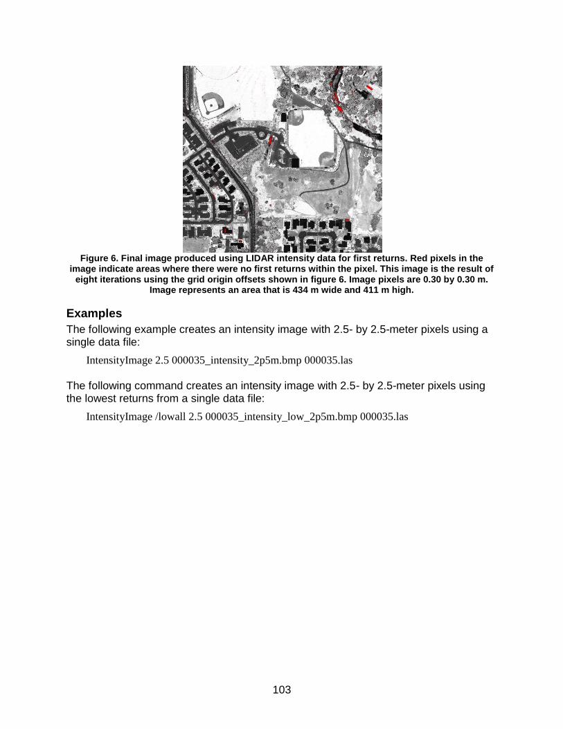
103

Figure 6. Final image produced using LIDAR intensity data for first returns. Red pixels in the

image indicate areas where there were no first returns within the pixel. This image is the result of eight iterations using the grid origin offsets shown in figure 6. Image pixels are 0.30 by 0.30 m.

Image represents an area that is 434 m wide and 411 m high.

Examples

The following example creates an intensity image with 2.5- by 2.5-meter pixels using a single data file:

IntensityImage 2.5 000035_intensity_2p5m.bmp 000035.las

The following command creates an intensity image with 2.5- by 2.5-meter pixels using the lowest returns from a single data file:

IntensityImage /lowall 2.5 000035_intensity_low_2p5m.bmp 000035.las

104

JoinDB

Overview

JoinDB merges merge two CSV files into a single file using a key field. This is a JOIN operation in database programs.

Syntax

JoinDB [switches] BaseFile BaseField AddFile AddField StartField OutputFile BaseFile Primary data file in CSV format. BaseField Field in the primary data file that will be matched to records in the

secondary data file. AddFile Secondary data file in CSV format. AddField Field in the secondary data file that will be matched to records in the

primary data file. StartField Starting field in the secondary data file. All fields (columns) starting with

the StartField will be added to records in the OutputFile. OutputFile Name for the new data file. The extension should be .csv. OutputFile

can be the same as BaseFile. OutputFile cannot be the same as AddFile.

Switches

noheader Treat the first line of the BaseFile and AddFile as data. Default behavior assumes the first line of each file contains column names. Valid for CSV format files only.

Technical Details

JoinDB performs a join operation using two data files. This is typically done in database systems but the capability was needed to implement object metrics for the output of TreeSeg. Initially, I wanted this to work with CSV and DBF formats but there are some limitations in DBF that may cause problems. Namely there is a limit of 255 fields. While this seems like it would work for most cases, the output from CloudMetrics with the /strata option with 9 height breaks produces 213 columns. Additional height breaks add 11 columns per strata so the limit of 255 columns would be reached with 12 height breaks.

Examples

The following command joins two CSV files, HighPoints.csv and SegmentMetrics.csv matching the value in column 3 in HighPoints.csv to those in column 1 of SegmentMetrics.csv. Columns starting with column 7 and beyond from SegmentMetrics.csv will be added to the outputfile (TreeMetrics.csv):

JoinDB HighPoints.csv 3 SegmentMetrics.csv 1 7 TreeMetrics.csv

105

LDA2ASCII

Overview

LDA2ASCII converts LIDAR data files into ASCII text files. It provides simple conversion capabilities for all LIDAR formats supported by FUSION. It was originally developed as a way to check the values being stored in LDA format files but still has utility as a conversion tool. It provides capabilities similar to the Tools…Data conversion…Export data from LAS or LDA formats to other formats… menu option.

Syntax

LDA2ASCII inputFile outputFile format [identifier] [noheader] inputFile Name of the input data file. Format must be LDA, LAS, or ASCII XYZ. outputFile Name for the output ASCII text file. format Format identifier:

0 X Y Elevation 1 Pulse Return X Y Elevation Nadir Intensity 2 FUSION-LTK CSV (X,Y,Elevation,Intensity,Pulse number,Return

number,Returns per pulse,Nadir angle) identifier Identifier for format 3 output, cannot include spaces (optional) noheader If zero, suppress the heading in the output file. Can only be used when

[identifier] is used

Technical Details

LDA2ASCII does not recognize the standard FUSION-LTK command line switches and it does not write entries to the FUSION-LTK master log file.

Examples

The following command converts an LDA file into ASCII text with X, Y, and Elevation values only:

LDA2ASCII 000263.lda 000263.txt 0

The following command converts an LAS file to the FUSION-LTK comma separated value (CSV) format:

LDA2ASCII 000263.las 000263.csv 2

106

LDA2LAS

Overview

LDA2LAS was originally developed to convert LIDAR data stored in FUSION’s LDA format to LAS format. When used with LDA format input, LDA2LAS writes LAS files that, while they can be read by most other programs that read LAS format, are not complete. Some of the fields for each return are not populated because the required information is not available in the LDA file. Specifically the field that details the number of returns for a pulse is always set to 0. This information would allow you to determine that a particular return is, for example, return 2 of 3 for the pulse. In addition, LDA2LAS will produce LAS files for LIDAR data that are missing items such as the GPS time, scan angle, and intensity. If you are producing data to be used by other people, you should not use the LAS files produced by LDA2LAS with LDA format input as they would lead people to think that all required fields in the LAS format specification are included. Command line programs were changed in FUSION release version 3.00 to output LAS format files when using LAS format input files. The LAS files produced by all command line programs (except LDA2LAS when using LDA format files for input) are complete and contain the projection information and other variable length records present in the source LAS format files. Output files will be written using the same LAS version as the first input LAS file and the variable length records from the first input LAS file will be copied to the output LAS file. When support for compressed LAS files was added to FUSION (Version 3.40), LDA2LAS provides the capability to act as a compression/decompression tool to convert between LAS and LAZ formats. When used for this purpose, the output LAS files are fully compliant with the LAS specification and should be readable by all programs that read LAS and LAZ format files.

Syntax

LDA2LAS [switches] InputFile OutputFile

InputFile Name of the input file. File must be in LDA, LAS or LAZ format. OutputFile Name for the output LAS format data file. Switches

cleanlas Only output points that adhere to the LAS format specification (valid GPS time, return # from 1 to 5, within header extent, points not flagged as withheld. Valid for LAS format input.

bylines Output a separate file for data from each flightline contained in the input file. The line number will be appended to the outputfile name. Files can contain data from a maximum of 256 flight lines. This option is only valid when the input files are in LAS or LAZ format.

107


Technical Details

Examples

The following example converts LIDAR data stored in LDA format into the LAS format:

LDA2LAS 000035.lda 000035.las

The following example compresses data stored in an LAS file into a file stored in the LAZ format develop by Martin Isenburg: LDA2LAS 42122-SW-AC.LAS 42122-SW-AC.LAZ

The following example decompresses data stored in the LAZ format into a standard LAS format file: LDA2LAS 42122-SW-AC.LAZ 42122-SW-AC.LAS

108

MergeData

Overview

MergeData combines several point cloud files into a single output file. The merge is accomplished by sequentially reading each input file and writing the point data to the output file.

Syntax

MergeData [switches] DataFile OutputFile DataFile LIDAR data file template or name of a text file containing a list of

file names (list file must have .txt extension). OutputFile Name for the output data file with extension. Switches


index Create FUSION index files for the output file. lda Write output files using FUSION's LDA format when using LAS

input files. The default behavior after FUSION version 3.00 is to write data in LAS format when the input data are in LAS format. When using input data in a format other than LAS, sample files are written in LDA format.



Technical Details

Data sampling in FUSION seems to be more efficient if all data for a project are contained in one file. Testing on various computers shows that, for some configurations, samples are created much faster when all point data are contained in one file. Merging data files is not recommended unless you are experiencing slow performance when using FUSION. MergeData only writes data in LDA format so the additional point information contained in LAS format files is lost when files are merged. Because MergeData simply reads point data from the input files and writes the data to the output file, it cannot reassemble pulse data when the returns for the pulse were separated into different data files. This happens when point cloud data are divided into “tiles” for processing and delivery to the client.

109

Many of the FUSION-LTK command line programs were not designed to handle more than 20 million data points in a single file. These programs may become unstable when used with very large files (more than 20 million points) or their performance may be poor. If you find it necessary to merge data to improve FUSION’s performance, maintain the original data files for use with FUSION-LTK programs.

Examples

The following command merges all LDA format data files in the current directory into a single file named alldata.lda and creates FUSION index files for the output file:

MergeData /index *.lda alldata.lda

110

MergeDTM

Overview

MergeDTM combines several PLANS format DTM files into a single output file. MergeDTM can merge hundreds of DTM files and is not limited by the amount of memory available on the computer, only the amount of disk space on the output device. MergeDTM provides the same capability as the Tools…Terrain model…Combine… menu option in FUSION except MergeDTM does not automatically fill voids areas in the final output model (FUSION provides an option to do this).

Syntax

MergeDTM [switches] OutputFile InputFile OutputFile Name for the output DTM file. If no extension is specified .DTM

will be used. InputFile DTM file template, name of a text file containing a list of DTM

file names (list file must have .txt extension), or a list of DTM file names.

Switches

cellsize:size Resample the input DTM data to produce an output DTM with size by size grid cells.

overlap:operator Specify how overlap areas (two or more input DTM files cover the same grid points) should be treated. Supported operators are:

average: average the value from the input file being processed with the value already present in the output file

min: use the minimum of the data from the input file being processed and the value already present in the output file

max: use the maximum of the data from the input file being processed and the value already present in the output file

add: add the data from the input file being processed to a values already present in the output file

new: use the data from the input file being processed to populate the grid point

verbose Provides detailed progress and status information as MergeDTM runs.

disk Merge the .DTM files to a disk file. The default behavior is to try to hold the merged model in memory but there can be problems when there is not quite enough memory for the model. Only use this option when attempts to merge models using the default method (without the /disk switch) fail.

precision:# Override the default precision for the merged output file. The default behavior is to use the highest precision of the input

111

models to establish the precision of the output model. Valid values for precision are: 0 2-byte integer 1 4-byte integer 2 4-byte floating point (C type: float) 3 8-byte floating point (C type: double)

nofill Do not fill holes in the merged DTM. This option should be used when merging DTM files that contain raster data (as opposed to surface data). The hole filling logic can end up adding data to areas not covered by the original input DTM files.

exactextent Preserve the exact extent of the input models in the output model. The default behavior is to expand the extent to the nearest multiple of the output cell size.

Technical Details

MergeDTM was designed to merge very large surface models consisting of several tiles. In operation, MergeDTM first scans the list of input models and determines the overall extent of the coverage area. The coverage area is expanded so the origin of the output model is a multiple of the output cell size. Then it verifies that there is sufficient space on the output storage device and creates an “empty” surface model file. The empty model is populated with NODATA values. Finally MergeDTM begins scanning the list of input models and uses them to populate portions of the output model. The value for the output model is interpolated from the input models so you can merge models with different cell sizes. In addition, the grids in the input models do not need to align. The default behavior of MergeDTM is to populate a grid point in the output model using the first input file that covers the point. Once a valid value has been stored for a grid point in the output model, it will not be overwritten even if subsequent input models cover the point. Use of the overlap area operator “new” changes this behavior. When the “new” operator is specified, points in the output model are populated using the last input model that covers the point. This operation allows you to “patch” a terrain model with new data by specifying the “patch” last in the list of input files. MergeDTM will try to create the output model in memory. If there is insufficient memory, it will create the model directly on the output device. Performance will be slower when the output model cannot be held in memory. MergeDTM will try to load each input model into memory as it is used to populate the output model. If the input model will not fit in available memory, it will be accessed from the disk as needed. Performance will be slower if the input models cannot be loaded into memory as they are needed. The worst case scenario for MergeDTM is when the output model is too large for memory and all of the input files are also too large for memory, i.e., combining several very large models. Performance in such situations may be very slow. Use of the /verbose option is encouraged to provide status messages describing the progress of the merge operation. MergeDTM looks at the cell size, coordinate system, measurement units and datums for the first input model and then compares all other input models to the first. MergeDTM

112

cannot combine models that use different coordinate systems, measurement units, or datums. MergeDTM uses the cell size of the first input model as the cell size for the output model. However, MergeDTM can merge models with different cell sizes. In such cases, the cell size of the first model is used for the output model and new values are interpolated from the input models. Use of the /cellsize:size switch forces MergeDTM to use the specified cell size for the output model regardless of the cell sizes in the input models.

Examples

The following example merges all of the DTM files in the current directory into a single model named combined.dtm:

MergeDTM combined.dtm *.dtm

The following example uses the data contained in the model file improved.dtm to “patch” the values in the model named original.dtm. The resulting “patched” model is stored in a file named patched.dtm:

MergeDTM patched.dtm original.dtm improved.dtm

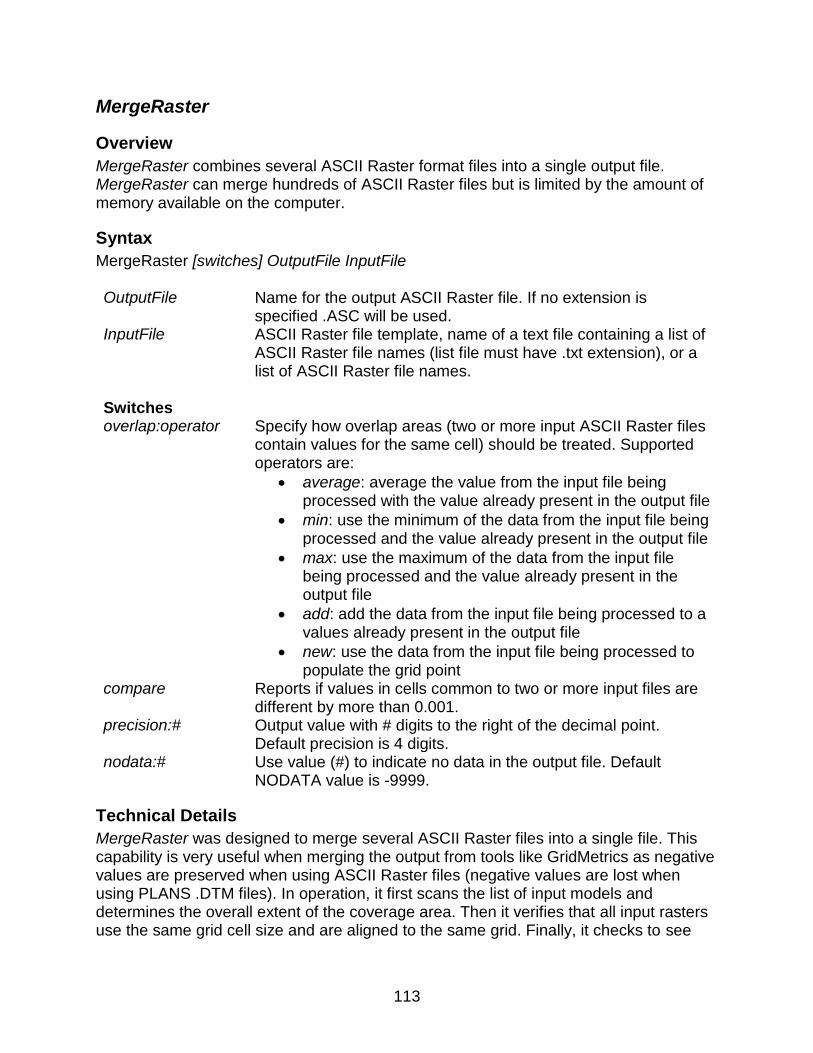
113

MergeRaster

Overview

MergeRaster combines several ASCII Raster format files into a single output file. MergeRaster can merge hundreds of ASCII Raster files but is limited by the amount of memory available on the computer.

Syntax

MergeRaster [switches] OutputFile InputFile OutputFile Name for the output ASCII Raster file. If no extension is

specified .ASC will be used. InputFile ASCII Raster file template, name of a text file containing a list of

ASCII Raster file names (list file must have .txt extension), or a list of ASCII Raster file names.

Switches

overlap:operator Specify how overlap areas (two or more input ASCII Raster files contain values for the same cell) should be treated. Supported operators are:

average: average the value from the input file being processed with the value already present in the output file

min: use the minimum of the data from the input file being processed and the value already present in the output file

max: use the maximum of the data from the input file being processed and the value already present in the output file

add: add the data from the input file being processed to a values already present in the output file

new: use the data from the input file being processed to populate the grid point

compare Reports if values in cells common to two or more input files are different by more than 0.001.

precision:# Output value with # digits to the right of the decimal point. Default precision is 4 digits.

nodata:# Use value (#) to indicate no data in the output file. Default NODATA value is -9999.

Technical Details

MergeRaster was designed to merge several ASCII Raster files into a single file. This capability is very useful when merging the output from tools like GridMetrics as negative values are preserved when using ASCII Raster files (negative values are lost when using PLANS .DTM files). In operation, it first scans the list of input models and determines the overall extent of the coverage area. Then it verifies that all input rasters use the same grid cell size and are aligned to the same grid. Finally, it checks to see

114

that there is sufficient space on the output storage device and creates an “empty” surface model file. The empty model is populated with NODATA values. Finally MergeRaster begins scanning the list of input rasters and uses them to populate portions of the output model. The default behavior of MergeRaster is to populate a cell in the output model using the first input file that covers the point. Once a valid value has been stored for a grid cell in the output model, it will not be overwritten even if subsequent input models cover the cell. Use of the overlap area operator “new” changes this behavior. When the “new” operator is specified, cells in the output model are populated using the last input model that covers the cell. This operation allows you to “patch” a raster with new data by specifying the “patch” last in the list of input files. MergeRaster looks at the cell size, and grid alignment for the first input raster and then compares all other rasters to the first. MergeRaster cannot combine models that use different grid cell sizes or that are not aligned to a common grid.

Examples

The following example merges all of the ASCII raster files with an extension of .ASC in the current directory into a single model named combined.asc:

MergeRaster combined.asc *.asc

The following example uses the data contained in the raster file improved.asc to “patch” the values in the raster named original.asc. The resulting “patched” model is stored in a file named patched.asc:

MergeRaster patched.asc original.asc improved.asc

115

PDQ

Overview

PDQ is a simple, fast data viewer for .LDA, .LAS, and .DTM files. PDQ supports drag-and-drop so you can drag data files onto an icon (shortcut) for PDQ or you can drop data files onto a running instance of PDQ. For point cloud data, PDQ automatically applies a color ramp to the data using the point elevations. The color ramp runs from brown (lowest) to green (highest).

Syntax

PDQ datafle

Datafile Name of the input data file. File must be in LDA, LAS, or PLANS DTM format.

Switches

m Allows multiple instances of PDQ. To use this option, you must run PDQ from a DOS command line.

s Synchronize multiple instances of PDQ so data manipulation in one instance will be mirrored in all other instances. To use this option, you must run PDQ from a DOS command line.

Technical Details

PDQ is written using a programming model similar to that used for computer games. It constantly redraws whether or not the user has adjusted the view or changed display settings. PDQ supports stereoscopic viewing using anaglyph, split-screen (parallel or cross-eyed viewing), or specialized stereo viewing hardware. While the user is manipulating the view, PDQ attempts to maintain a refresh rate of 30 frames/second. To do this, point data is divided into 32 layers and PDQ only draws as many layers as it can while maintaining the desired frame rate. For surface models, PDQ creates a low-resolution version of the surface model and draws this version when the user is manipulating the view. For both data types, the full-resolution data are rendered whenever the user stops manipulating the view. To use stereo viewing hardware, the hardware must be capable of supporting OpenGL quad-buffered stereo. When PDQ starts, it will look for stereo hardware and use it if available. If you prefer that PDQ run in monoscopic mode, you will need to disable the stereo hardware using the display driver configuration utility provided by the hardware (graphics card) manufacturer. PDQ is very useful for checking both point cloud data and surface model data. For maximum convenience, the .LDA, .LAS, and .DTM file extensions can be associated with PDQ. Then users simply need to double-click a data file to have it displayed in PDQ.

116

PDQ offers a scanning mode that can be used to examine large ground or canopy surface models. This mode is initiated by pressing F5 when a .DTM file is loaded into the viewer. The (+) and (-) keys move the surface model left and right and the Z and shift-Z keys move the model up and down. The zoom feature (mouse wheel) can be used to zoom into or away from the surface model. PDQ can also provide specialize coloring for LAS point files. Colors are assigned to individual points based on the classification field in the LAS data records. For the list of colors assigned to codes, see the Help…about dialog in PDQ. PDQ can display different data sets in different windows and synchronize movement of the windows. To launch a “clone” window while PDQ is running, use the Clone PDQ menu option. You can then drag a data file into the new window for viewing. To run multiple copies of PDQ from a command prompt, use the /m switch. To synchronize movement in multiple copies, use the /s switch along with the /m switch. The following keystroke commands are available in PDQ:

117


Description

Left mouse button and mouse movement

Manipulate the PDQ data display. The viewing model assumes that the data is inside a glass ball. To manipulate the view, hold down the left mouse button and roll to “glass ball”.

Mouse wheel Zoom in and out.

Escape Stop data rotation (only when continuous rotation mode is enabled).

A Toggle anaglyph mode.

B Set background color to black.

E Decrease eye separation in split-screen stereo modes.

Shift & E Increase eye separation in split-screen stereo modes.

Shift & Ctrl & E Reset eye separation to default value in split-screen stereo modes.

I Toggle display of axes (wireframe cube).

L Toggle coloring by LAS classification values (LAS data files only).

M Toggle continuous rotation mode. When this is on, the data cloud or surface continue to move after the user releases the left mouse button.

N Toggle coloring using intensity data from LAS files (if available).

O Reset the orientation of the view to an overhead view.

R Begin/end recording an AVI video file.

S Toggle split-screen stereo mode.

Ctrl & T Capture the current screen image to a file.

W Set the background color to white

X Toggle between cross-eyed and parallel viewing in split-screen stereo mode.

Z Lower the DTM model while in scanning mode.

Shift & Z Raise the DTM model while in scanning mode.

Ctrl & + (plus key) Increase the symbol size.

Ctrl & - (minus key)

Decrease the symbol size.

F5 Toggle scanning mode for DTM evaluation (use + and – along with and shift-Z to move model).

Examples

The following command displays the data file named tile20023.lda using PDQ:

PDQ tile0023.lda

118

PolyClipData

Overview

PolyClipData clips point data using polygons stored in ESRI shapefiles. The default behavior of PolyClipData is to produce a single output file that contains all points that are inside all of the polygons in the shapefile. Optional behaviors include including only points outside the polygons, producing individual files containing the points within each polygon in the shapefile, and clipping points within a single polygon specified using a field from the shapefile database.

Syntax

PolyClipData [switches] PolyFile OutputFile DataFile PolyFile Name of the ESRI shapefile containing polygons. Only polygon

shapefiles can be used with PolyClipData. OutputFile Base name for output data files. Default behavior is to create

one output file named OutputFile that contains all of the points within all of the polygons in PolyFile.

DataFile LIDAR data file template or name of a text file containing a list of file names (list file must have .txt extension).

Switches

index Create FUSION index files for the output file. outside Create output file containing all points outside of all polygons in

PolyFile. When used with /shape switch, output file will contain all points outside the specified polygon.

multifile Create separate output data files for each polygon in PolyFile. shape:field#,value Use the feature in PolyFile identified by value in field field#.

Output file will contain all points within the specified polygon. field# is a 1-based index that refers to fields in the DBASE file associated with the shapefile. The /shape switch is ignored for other formats. If the polygon identifier contains a space, enclose the identifier in quotes. Use a “*” for value to force indexing of the polygon file and parse polygon identifiers from field#. If you do not use the /shape switch in conjunction with the /multifile switch, output files will be identified using the sequential number associated with the polygon rather than a value from a database field.

119

class:string Used with LAS format files only. Specifies that only points with classification values listed are to be included in the output. Classification values should be separated by a comma e.g. (2,3,4,5) and can range from 0 to 31. If the first character of string is “~”, all classes except those listed will be used.




Technical Details

PolyClipData recognizes only ESRI shapefiles containing polygons. Polygons can be simple, one-part shapes, multi-part polygons, or polygons with holes. To ensure accurate clipping, the shapefile should be “cleaned” in ArcInfo to ensure that the arrangement of polygons and especially holes in polygons are correctly arranged and ordered. When used with the /multifile switch, PolyClipData produces a separate point file for each polygon. PolyClipData tries to minimize the number of times the point data area read during the clipping process. However, due to limitations with the programming language used for PolyClipData, only 64 polygons can be used at once. This means that PolyClipData may need to divide the polygons into groups a 64 and process each group using a separate pass through the point data. This process is transparent to the user except for the status messages indicating that only a portion of the polygons are being processed.

Examples

The following command clips all points in tile0023.lda that are inside to polygons contained in stand_polys.shp and saves them in a single file names stand_pts_tile0023.lda:

PolyClipData stand_polys.shp stand_pts_tile0023.lda tile0023.lda

The following command clips points from tile0023.lda that are inside of polygons identified by the value “plantation” in the fourth column of the shapefile database for stand_polys.shp and stores the point data in a file named plantations.lda:

PolyClipData /shape:4,plantation stand_polys.shp plantations.lda tile0023.lda

120

The following command clips points from tile0023.lda that are inside polygons stored in stand_polys.shp creating a separate file for point inside each stand polygon. Output files are labeled using the values in the third column of the shapefile database.

PolyClipData /shape:3,* stand_polys.shp stand.lda tile0023.lda

121

RepairGridDTM

Overview

RepairGridDTM creates a new set of DTM tiles for datasets where the set of DTM tiles do not provide full coverage for the area. This occurs most often when DTMs are delivered in a raster format where the vendor has not considered the correct alignment of the cells in adjacent tiles. Basically, the DTMs have been treated as raster data where the entire cell is represented by the value for the cell instead of lattice data where the values represent points located at the center of each cell. When the individual files are interpreted as surfaces, there is a 1 cell gap between adjacent tiles.

Syntax

RepairGridDTM [switches] groundfile extraspace groundfile File specifier for ground surface models in PLANS DTM format.

May be wildcard or text list file (extension .txt only). Normally this will specify all DTM files for a project area or acquistition.

extraspace Distance added around all sides of a DTM tile. Same units as the source groundfiles.

Switches

The standard FUSION-LTK toolkit switches are supported,

Technical Details

Bare ground surface models delivered in ARC GRID format (or other raster formats) assume that the elevation represents the entire cell instead of a single point. In ArcInfo, the lattice structure is more appropriate. When converted to ASCII raster format, the location of the lower left corner of the lower left cell is reported in the ASCII raster header. When FUSION converts the ASCII raster file into the PLANS DTM format, it understands that the elevation value is actually a point sample for the ground surface and adjusts the origin of the model to the center of the lower left cell (Figure 7). This behavior is fine for a single model. However for two adjacent models the result is a 1-cell gap between the extents of the two models (Figure 8). If the two or more models are merged, FUSION interpolates elevations to fill the gap. However, if the two models are maintained as separate files for subsequent use, the gap will remain and any program that tries to use the model will “see” the gap and report that there are no valid elevations for the area covered by the gap. This is especially problematic when we want to use the model to normalize the LIDAR return elevations relative to the ground elevation (produce a return height instead of return elevation). Programs like GridMetrics can produce results with distinct stripes that correspond to the gaps between models.

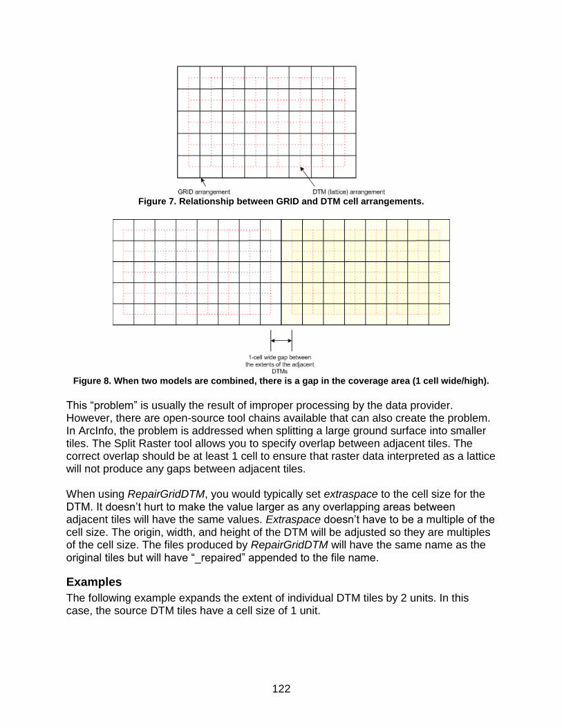
122

Figure 7. Relationship between GRID and DTM cell arrangements.

Figure 8. When two models are combined, there is a gap in the coverage area (1 cell wide/high).

This “problem” is usually the result of improper processing by the data provider. However, there are open-source tool chains available that can also create the problem. In ArcInfo, the problem is addressed when splitting a large ground surface into smaller tiles. The Split Raster tool allows you to specify overlap between adjacent tiles. The correct overlap should be at least 1 cell to ensure that raster data interpreted as a lattice will not produce any gaps between adjacent tiles. When using RepairGridDTM, you would typically set extraspace to the cell size for the DTM. It doesn’t hurt to make the value larger as any overlapping areas between adjacent tiles will have the same values. Extraspace doesn’t have to be a multiple of the cell size. The origin, width, and height of the DTM will be adjusted so they are multiples of the cell size. The files produced by RepairGridDTM will have the same name as the original tiles but will have “_repaired” appended to the file name.

Examples

The following example expands the extent of individual DTM tiles by 2 units. In this case, the source DTM tiles have a cell size of 1 unit.

123

ReturnDensity

Overview

ReturnDensity produces raster outputs containing the number of returns in each cell. This type of output can also be produced using the Catalog utility but ReturnDensity is more efficient and only produces the return count layer. Output from ReturnDensity is useful in the LTKProcessor and AreaProcessor workflow tools to help subdivide large acquisitions into manageable chunks for processing. ReturnDensity also produces percentile values for first return intensity values. These are useful for establishing scaling values when creating intensity images or comparing intensity values for different acquistitions.

Syntax

ReturnDensity [switches] outputfile cellsize datafile1 datafile2... outputfile Name for output raster file (stored in PLANS DTM format with

.dtm extension). cellsize Desired grid cell size in the same units as LIDAR data. datafile1 First LIDAR data file (LDA, LAS, ASCII LIDARDAT

formats)...may be wildcard or name of text file listing the data files. If a wildcard or text file is used, no other datafile# parameters will be recognized.


Switches

first Use first returns when computing return counts (default is all returns).

ascii Output raster data in ASCII raster format instead of PLANS DTM format. Output file extension will be “.asc”.

nointpercentile Do not compute percentile values associated with first return intensity and output to CSV file. These values are useful to determine the range of values to scale intensity products.

projection:filename Associate the specified projection file with ASCII raster products.

class:string LAS files only: Specifies that only points with classification values listed are to be included in the subsample. Classification values should be separated by a comma, e.g., (2,3,4,5) and can range from 0 to 31. If the first character of string is “~”, all classes except those listed will be used.

124

grid:X,Y,W,H Force the origin of the output grid to be (X,Y) instead of computing an origin from the data extents and force the grid to be W units wide and H units high...W and H will be rounded up to a multiple of CellSize.

gridxy:X1,Y1,X2,Y2 Force the origin of the output grid to be (X1,Y1) instead of computing an origin from the data extents and force the grid to use (X2,Y2) as the upper right corner of the coverage area. The actual upper right corner will be adjusted to be a multiple of CellSize.

align:filename Force the origin and extent of the output grid to match the lower left corner and extent of the specified PLANS format DTM file.

extent:filename Force the origin and extent of the output grid to match the lower left corner and extent of the specified PLANS format DTM file but adjust the origin to be an even multiple of the cell size and the width and height to be multiples of the cell size.

Technical Details

ReturnDensity is typically used to produce a raster layer containing point density information and a csv file containing percentile values for first-return intensity. It produces the same output as produced by the Catalog utility when the /rawcounts and /density options are used. The output from ReturnDensity can be used along with LTKProcessor to develop an arrangement of processing tiles that contain a specific number of returns. By default, the output contains the total number of returns in each cell. Using the /first switch outputs only the number of first returns in each cell. ReturnDensity displays some of the intensity percentile values on the command line and produces a CSV file containing all percentile values.

Examples

The following example produces a raster file (stored in .DTM format) containing the number of first returns in each 5 by 5-unit cell:

ReturnDensity /first pulsedensity.dtm 5 *.las

The following example produces a raster file (stored in .DTM format) containing the number of returns (all returns) in each 5- by 5-unit cell:

ReturnDensity pulsedensity.dtm 5 *.las

125

SplitDTM

Overview

SplitDTM divides a .DTM file into smaller tiles. It is most often used when bare-ground surface models are delivered in large tiles that cannot be managed efficiently. The command-line tools in FUSION all provide the ability to work with multiple ground surface files. In operation, the tools either build new, temporary grids covering the area of interest or access the ground models from disk. When creating workflows for processing data covering large areas, LTKProcessor allows users to specify the maximum number of returns in a processing tile. For datasets where the ground model tiles are large, some tools have problems loading the large models while trying to build a temporary model to support the analysis tasks. The result is that the programs start to page data in and out of memory and performance suffers by several orders of magnitude. By subdividing large ground tiles into smaller tiles, memory is used more efficiently and the paging behavior is avoided. SplitDTM offers two ways to specify the arrangement of the new tiles. In the first, the user specifies the number of rows and columns of new tiles and for the second the user specifies the maximum number of cells in a new tile. SplitDTM provides a default maximum number of cells (25 million) that produces tiles that are about 100Kb and cover an area that is 5000 by 5000 cells. This size seems to work well with all processing tools and improves the overall processing efficiency.

Syntax

SplitDTM [switches] inputDTM outputDTM columns rows inputDTM Name of the existing PLANS format DTM file to be subdivided. outputDTM Base name for the new PLANS format DTM tiles. The actual tile name

will have the column and row appended to it. columns Number of columns of tiles. rows Number of rows of tiles. Switches

maxcells:[#] Maximum number of cells in the output tiles. When this option is used, the column and row parameters are ignored but values for them are needed on the command line. The number of columns and rows will be calculated to produce tiles that contain fewer that the specified number of cells. The default maximum number of cells is 25,000,000.

Technical Details

SplitDTM is a simple program that was designed to help improve processing efficiency for large areas. When the user specifies the number of columns and rows of output tiles, the program simply cuts the large inputDTM into the needed number of tiles. It does not evaluate the tiles to see if they contain valid data so it is possible, when the coverage area within a large tile does not cover the full extent of the tile, to produce tiles that are filled with NODATA values. If the user uses the /maxcells option, the logic in SplitDTM tries to produce reasonably square tiles that do not exceed the size constraint. The logic

126

that calculates the number of columns and rows is not perfect. In some cases, SplitDTM will produce more tiles that it needs to but all tiles will contain valid data and have fewer that the maximum number of cells. For example, it might split an area into 24 tiles when it could have split it into 22 tiles and still met the size constraint. In all cases, the tiles created by SplitDTM can be merged together to create a model that is identical to the original (except the model description will be changed to reflect the use of the SplitDTM and MergeDTM tools) using the MergeDTM tool. The inputDTM and outputDTM names can be the same since SplitDTM appends the column and row numbers to the tiles it creates.

Examples

The following example splits a large surface model into 20 smaller tiles:

SplitDTM q557432.dtm q5574232_tiles.dtm 4 5

The following example splits a large model into smaller tiles based on the default maximum number of cells in the output tiles (note that you must still include the column nd row parameters on the command line when using the /maxcells option):

SplitDTM /maxcells q557432.dtm q557432.dtm 1 1

The following example splits a large model into smaller tiles based on a specifc maximum number of cells in the output tiles:

SplitDTM /maxcells:40000000 q557432.dtm q557432.dtm 1 1

127

SurfaceSample

Overview

SurfaceSample produces a comma separated values (CSV) file that contains a value interpolated from the surface at a specific XY location. Input is a file containing a list of XY coordinate pairs, one pair per line of the file. Output is a CSV file containing the original XY location and the surface value. Optionally SurfaceSample can generate a network of radial profiles given center point, the number of radial lines, length of each line and the desired point spacing. SurfaceSample can also generate a series of evenly spaced sample points along a line specified by two endpoints. The formats of the input and output files vary depending on the options used.

Syntax

SurfaceSample [switches] surfacefile inputfile outputfile surfacefile Name for surface model (PLANS DTM with .dtm extension). inputfile Name of the ASCII text file containing the XY sample locations. This

file can be in CSV format including a header line to identify data columns. If a header is included, column names should not start with numbers. The XY values can be separated by spaces, commas, or tabs. If the /pattern option is used with type 3, the inputfile should contain two coordinate pairs that specify the endpoint of the line. If the /id option is used, the inputfile should contain a point identifier in the first column.

outputfile Name for the output data file. Output is stored in CSV format. The format and arrangement of the output data varies depending on the use of the /id and /pattern options.

Switches

pattern:type,p1,p2,p3

Generate a test pattern of sample points centered on the XY location from the inputfile. Pattern type 1 is a radial network of p1 lines that are p2 long with sample points every p3 units. The first radial is at 3 o’clock and radials are generated in counter-clockwise order. Pattern type 2 is a radial network of p1 lines that are p2 long with sample points every p3 units ON AVERAGE. The sample point spacing decreases as the distance from the XY location increases to provide sample point locations that represent a uniform area. The first radial is located at 3 o’clock and radials are generated in counter-clockwise order.

128

Pattern type 3 expects two coordinate pairs in the input data. The pairs specify the endpoints of a line. Lines with points spaced p1 units apart are created and written to the output.

topo:dist,lat Compute and output a solar radiation index (SRI) based on Keating et al. (2007). The algorithm for SRI uses a three- by three-cell grid where each grid cell is dist by dist units to compute topographic attributes. Then the slope and aspect are combined with the input latitude (lat) to compute SRI. When /topo:dist,lat is specified, output includes the slope, aspect, profile curvature (along the slope), plan curvature (across the slope), and SRI. Latitude values are positive for the northern hemisphere and negative for the southern.

noheader Suppress the header line in the outputfile. This option is useful when you want to use PDQ to view the outputfile.

novoid Suppress output for XY sample points outside the surface extent or for points with invalid surface elevations.

id Read a point identifier from the first field of each line from the inputfile and output it as the first field of the outputfile. If id is used with pattern, a separate output file is created for each point in the inputfile. Output files are named using outputfile as the base name with the point identifier appended to the filename. Even when inputfile contains a single point, the outputfile name is modified to reflect the point identifier.

Technical Details

SurfaceSample interpolates a value from a surface for each input XY location. If the XY location is outside the extent of the grid file, the value is set to -1.0 and output to the outputfile. The input file can be a single XY coordinate, a simple list of XY coordinates, or a list of identifiers and XY coordinates. If the input file contains a header in the first line of the file, the column labels cannot start with numbers. If they do, they first line of data in the output file will contain erroneous data. The output CSV file reports the surface value with 6 decimal digits for surface files that contain floating point values and with 0 decimal digits for surface files that contain integer values. When SurfaceSample is used with the /topo:dist,lat switch, a solar radiation index (SRI) and other topographic indices are computed for each input point. SRI combines information about the aspect, slope, and latitude into a single index that describes the amount of solar radiation theoretically striking an arbitrarily oriented surface during the hour surrounding noon on the equinox (Keating et al. 2007). The parameters for the topo switch define the size of the surface cell and the latitude for the study area. In operation, elevations are interpolated for points defining a three- by three-cell grid where each grid cell is dist by dist units. These elevations are then used to compute the slope, aspect, and curvature for the surface patch (Zevenbergen and Thorne 1987). For

129

most applications, the distance (or cell size) should not be small. The overall goal is to describe the terrain shape and not to capture every micro-topographic detail. SRI as defined by Keating et al. (2007) ranges from -1.0 to 1.0 but the full range is not possible at every location due to the effect of latitude on the index. For SurfaceSample, this range has been adjusted to range from 0.0 to 2.0. SRI does not consider the change in the amount of solar radiation that occurs over the course of a day or year or changes that result from topographic shading. However distills information about slope, aspect, and latitude into a single linear value useful for comparing locations. When topo is specified, output includes the slope, aspect, profile curvature (along the slope), plan curvature (across the slope), and SRI all reported with 6 decimal digits regardless of the storage type for the elevations in the surface model. The formula used to compute SRI (adapted from Keating et al. 2007) is:

aspectslopelatitudeslopelatitudeSRI cos*sin*sincos*cos0.1

where: latitude is the latitude in degrees with north latitudes positive and south latitudes

negative slope is the inclination of the surface from the horizontal position in degrees aspect is the surface azimuth angle in degrees relative to south (180.0 – calculated

aspect) When SurfaceSample is used with the pattern switch and pattern types 1 and 2, each radial line contains the surface value for the XY location from the inputfile (i.e. the center point) followed by sample points for the first line of the radial pattern. Radial lines start at 3 o’clock and proceed in counter-clockwise order. The length of each radial line is at least p2 units long (length is rounded up to be an even multiple of the point spacing (p3)). If the /id option is used, separate files are created for each center point and the identifier for each point includes the identifier read from the inputfile and an identifier for the radial line. When SurfaceSample is used with the pattern switch and pattern type 3, the inputfile should consist of two coordinate pairs. The output contains evenly-spaced points (spacing specified using p1) starting with the first coordinate pair and ending with the second pair. Point spacing between the last and next to last points may not match the value specified by p1.

Examples

The following example reads locations from the file named plotsSE.txt and outputs surface values interpolated the surface bare_ground.dtm into the outputfile named plot_elevations.csv.

SurfaceSample bare_ground.dtm plotsSE.txt plot_elevations.csv

The inputfile, plotsSE.txt contains the following records:

524750.0,5200000.0

524750.0,5200250.0

130

524750.0,5200500.0

524750.0,5200750.0

524750.0,5201000.0

525000.0,5200000.0

525000.0,5200250.0

525000.0,5200500.0

525000.0,5200750.0

525000.0,5201000.0

The outputfile, plot_ elevations.csv contains the following values (values were truncated to one decimal place for this example):

X,Y,Value

524750.0,5200000.0,156.2

524750.0,5200250.0,162.5

524750.0,5200500.0,-1.0

524750.0,5200750.0,-1.0

524750.0,5201000.0,-1.0

525000.0,5200000.0,146.9

525000.0,5200250.0,143.9

525000.0,5200500.0,-1.0

525000.0,5200750.0,-1.0

525000.0,5201000.0,-1.0

The following examples generate a sample of points along radial lines around a single XY location (stored in single_plot.csv). There are 8 lines that are 85 meters long. The first command line creates evenly-spaced sample points every 1 meter and the second creates points spaced to represent equal areas:

SurfaceSample /pattern:1,8,85,1 bare_ground.dtm plotsSE.txt single_plot.csv

SurfaceSample /pattern:2,8,85,1 bare_ground.dtm plotsSE.txt single_plot.csv

Output as displayed in PDQ is shown below (uniformly spaced on the left and equal-area on the right).

131

SurfaceStats

Overview

SurfaceStats computes surface area and volume under the surface (or between the surface and the ground) for an entire surface. Output is a single set of values stored in a CSV format file.

Syntax

SurfaceStats [switches] inputfile outputfile inputfile Name for the input DTM surface file including the .dtm extension. outputfile Name for the output CSV file containing the surface statistics. Switches

ground:file Use the specified surface model to represent the ground surface file may be wildcard or text list file (extension .txt only). A value interpolated from the file will be subtracted from every grid point in the inputfile.

Technical Details

SurfaceStats is useful for computing measures of canopy surface roughness and volume for small areas such as sample plots. It computes a single set of values for the entire area covered by the inputfile. Surface area and volume are computed by dividing each grid cell in the surface into two triangles from the lower left to the upper right corner. Then the area of each triangle is computed using the 3D coordinates of the triangle vertices. Area is the magnitude of the cross product of the three vertices. Volume under the surface for each triangle is computed by multiplying the flat triangle area (1/2 of the grid cell area) by the average elevation (or height) of the three vertices. Totals for the entire surface are simply the sum of the values for each triangle. Area and volume are only computed when all four corners of a cell in the inputfile have valid data. If any vertex has an invalid elevation (or height), the area and volume for the entire cell is 0.0.

132

SurfaceStats computes and outputs the following values:

Value Description Upper surface (canopy) Name of the input surface file Lower surface (ground) Name of the ground file specified with the /ground

switch Min X Minimum X in the input surface Min Y Maximum X in the input surface Min Elev Minimum Y in the input surface Max Elev Maximum Y in the input surface Columns Number of columns in the input surface Rows Number of rows in the input surface Cell Width Width of each cell in input surface Cell Height Height of each cell in input surface Overall Planimetric Area Total horizontal area covered by the surface

(includes areas with invalid elevations (or heights) Planimetric Area (Data only)

Total horizontal area covered by cells with valid elevations (or heights).

Upper Surface Area Total area of the surface Volume Under Upper Surface

Total volume under the surface

Examples

The following example computes the surface area and volume for the canopy model stored in PLOT1139.DTM and writes the values to the CSV file named PLOTSUMM.CSV:

SurfaceStats PLOT1139.DTM PLOTSUMM.CSV

ThinData

Overview

ThinData allows you to thin LIDAR data to specific pulse densities. This capability is useful when comparing analysis results from several LIDAR acquisitions that were collected using different pulse densities. ThinData is also useful when the density within a single LIDAR data set is not uniform. This is often the case with data collected from a slow-flying helicopter or when flightline overlap was not closely monitored. ThinData has also been used in simulation experiments to assess the effect of LIDAR pulse density on the accuracy of estimated forest inventory metrics such as overall tree height.

Syntax

ThinData [switches] OutputFile Density CellSize DataFile

OutputFile The name of the output LIDAR data file containing the new dataset thinned to the desired density.

133

Density Desired pulse density per square unit.

CellSize The cell size used to compute data density specified in square units.



Switches

rseed:# Use random number stream #. ThinData provides 100 different streams of random numbers so # can range from 0 to 99.

index Create FUSION index files for the thinned data file.





Technical Details

ThinData is designed to produce output data sets that have uniform pulse densities throughout the coverage area. To accomplish this, ThinData first scans the entire dataset specified by DataFile and computes pulse density using the specified CellSize. For each cell, the proportion of pulses that will be retained is computed using the calculated pulse density and the desired pulse density. Logic within ThinData identifies a new pulse whenever it encounters a new first return or when it encounters a 2nd, 3rd, 4th, .etc. return without a corresponding 1st, 2nd, 3rd, etc. return. ThinData does not use the FUSION index files to read data as this could lead to separation of returns from the same pulse when the returns occur in different tiles within the indexing grid.

134

In general it is best to use a large CellSize to compute the pulse densities (25 m2 or larger). Smaller cells can be used but it will be harder to obtain specific pulse densities if only a few pulses are contained in each cell. Experience using ThinData has shown that it algorithm will generally produce output datasets with pulse densities within 1 to 3 percent of the specified Density. When using the /class:string switch, ThinData uses all returns to determine the pulse structure and then thins the pulses. However, only returns from a pulse included in the thinned data with classification values that match those specified in the /class:string switch are written to the output file.

Examples

The following command thins and indexes a dataset consisting of all .lda files in the current directory to 5 pulses/meter2 computed using a 25 meter2 cell (5- by 5-meter):

ThinData /index newdata.lda 5 25 *.lda

TiledImageMap

Overview

TiledImageMap creates a web page consisting of a single image map that corresponds to a mosaic of image tiles. The image map is linked to individual tile images allowing the user of the page to browse the coverage area switching between the larger overview image and the higher-resolution individual image tiles. For colored overview images, a legend image that describes the image can be included. TiledImageMap is most often used to organize intensity images created from LIDAR data but it can be used to provide web-ready display of any spatial information that is organized into tiles. TiledImageMap is particularly useful when LIDAR data have been delivered in “tiles” and subsequent data products have been produced using files representing individual “tiles”. Creating web pages with TiledImageMap makes it easy to browse analysis results and facilitates access to analysis products without using GIS.

Syntax

TileImageMap [Switches] OutputHTML IndexImage TileTemplate OutputHTML Name for the output HTML page (extension is not needed). IndexImage Name of the large image used to create the image map. The image

must have a corresponding world file to provide coordinate system information.

TileTemplate File template for image tiles or the name of a text file containing a list of image tiles.

Switches

Legend:file Add a legend image to the HTML page to the left of the image map. file is the name of the image to use for the legend.

135

Technical Details

TiledImageMap uses the world files for the IndexImage and the individual tile images to locate the tile images within the area represented in the IndexImage. All images must have world files. The web page created by TiledImageMap allows you to click on the area of the IndexImage and display the corresponding tile image. The IndexImage is shown at the top of the page with the legend (if specified) located below the IndexImage.

Examples

The following example creates a web page that contains the results of canopy cover analyses done using Cover:

TiledImageMap CoverSummary.html MergedCover.jpg cover*.jpg

136

TINSurfaceCreate

Overview

TINSurfaceCreate creates a gridded surface model from point data. The algorithm used in TINSurfaceCreate first creates a TIN surface model using all of the points and then interpolates a gridded model from the TIN surface. TINSurfaceCreate works well when all points in a dataset are to be used as surface points. For example, after filtering a LIDAR point cloud to identify bare-ground points, TINSurfaceCreate can be used to create a gridded surface model. However, if any non-ground points remain in the dataset, they will be incorporated into the TIN ground surface model and will, most likely, affect the resulting gridded surface model. In general, TINSurfaceCreate should be used only when you know all points in the dataset are surface points. If this is not the case, use GridSurfaceCreate to create the gridded surface model.

Syntax

TINSurfaceCreate [switches] surfacefile cellsize xyunits zunits coordsys zone horizdatum vertdatum datafile1 datafile2... surfacefile Name for output surface file (stored in PLANS DTM format with .dtm

extension). cellsize Grid cell size for the surface in the same units as the LIDAR data. xyunits Units for LIDAR data XY:








datafile2 Second LIDAR data file (LDA, LAS, ASCII LIDARDAT formats).

137

Several data files can be specified. The limit depends on the length of each file name. When using multiple data files, it is best to use a wildcard for datafile1 or create a text file containing a list of the data files and specifying the list file as datafile1.

Switches

return:string Specifies the returns to be included in the sample. String can include A,1,2,3,4,5,6,7,8,9,F,L. A includes all returns. For LAS files only: F indicates first and only returns, L indicates last of many returns. F and L will not work with non-LAS files.


Technical Details

TINSurfaceCreate uses triangulation algorithms developed by Jonathan Richard Shewchuk at the University of California at Berkeley5. These algorithms comprise are one of the fastest, most robust triangulation applications available and were well suited for use with millions of data points. When creating a gridded surface model from the TIN, TINSurfaceCreate uses special logic near the edges of the TIN surface to prevent interpolation anomalies in the output grid. For data that is processed in tiles, most edge-matching problems are minimized using this approach. If your data is stored in tiles, you can process each tile to produce a gridded surface model and then combine the models using the Tools menu in FUSION or the MergeDTM utility. As tiles are combined, edge areas will contain voids if the TIN surface did not extend fully to the data extent. After combining tiles, the logic in FUSION, scans the final model looking for void areas and fills these areas by interpolating from surrounding grid values. As stated in the overview, non-ground points included in the input data will have an effect on the final gridded surface. The magnitude of the effect will depend on the number of non-ground points and their distribution. Single non-ground points will likely influence the final surface only slightly. However, groups of non-ground points will cause significant “bumps” in the final surface.

Examples

The following example creates a gridded surface model with a 2.5- by 2.5-meter cell using the point data stored in tile0023_groundpts.lda:

TinSurfaceCreate tile0023_ground.dtm 2.5 m m 1 10 2 2 tile0023_groundpts.lda

5 http://www.cs.cmu.edu/~quake/triangle.html last visited September 9, 2009.

138

TopoMetrics

Overview

TopoMetrics computes topographic metrics using surface models. The logic it uses is exactly the same as that used in GridMetrics except TopoMetrics computes a topographic position index (TPI) based on methods described by Weiss (2001) and Jenness (2006).

Syntax

TopoMetrics [switches] SurfaceFile CellSize TopoPointSpacing Latitude TPIWindowSize OutputFile

SurfaceFile Name for the input surface file (PLANS DTM format). SurfaceFile may be wildcard or text list file (extension .txt).

CellSize Size of the cell used to report topographic metrics TopoPointSpacing The spacing for the 3 by 3 array of points used to compute the

basic topographic metrics. Latitude Latitude for the center of the data area. North latitude is

positive, South is negative. Latitude is used to compute the solar radiation index.

TPIWindowSize The size of the window used to compute the topographic position index. When the /square option is used, the TPI window will be TPIWindowSize by TPIWindowSize. For round windows, the diameter will be TPIWindowSize.

OutputFile Base name for the output metrics (CSV format). "_topo_metrics" will be appended to the name provided on the command line.

Switches grid:X,Y,W,H Force the origin of the output grid to be (X,Y) instead of

computing an origin from the data extents and force the grid to be W units wide and H units high...W and H will be rounded up to a multiple of CellSize.

gridxy:X1,Y1,X2,Y2 Force the origin of the output grid to be (X1,Y1) instead of computing an origin from the data extents and force the grid to use (X2,Y2) as the upper right corner of the coverage area. The actual upper right corner will be adjusted to be a multiple of CellSize.

align:filename Force the origin and extent of the output grid to match the lower left corner and extent of the specified PLANS format DTM file.

extent:filename Force the origin and extent of the output grid to match the lower left corner and extent of the specified PLANS format DTM file but adjust the origin to be an even multiple of the cell size and the width and height to be multiples of the cell size.

square Use a square-shaped mask when computing the topographic position index. The default mask shape is a circle.

139

annulusinnerdia:dia Use a donut-shaped mask when computing the topographic position index. The outer diameter is TopoDistance and the inner diameter is dia. When using this option to define a narrow ring, use the /verbose option to display the computed mask to ensure it meets your expectations.

annuluswidth:width Use a donut-shaped mask when computing the topographic position index. The outer diameter is TPIWindowSize and the inner diameter is TPIWindowSize-(width*2). When using this option to define a narrow ring, use the /verbose option to display the computed mask to ensure it meets your expectations.

diskground Do not load ground surface models into memory or create a temporary surface in memory. When this option is specified, larger areas can be processed but processing will be very much slower.

nointernalground Do not create a temporary surface in memory. When this option is specified, larger areas can be processed but processing will be much slower. This option has no effect when used with /diskground.

lockdtmcellsize Force the cell size used when creating an internal ground model to be the same as the highest resolution input ground surface model. The default behavior will increase the cell size until the internal model will fit in the available memory.

Technical Details

TopoMetrics uses the same logic as GridMetrics to compute topographic metrics. The additional output: topographic position index (TPI) is calculated using a moving window centered on the grid-cell center. The size of the window is controlled by the TPIWindowSize parameter. The default window is circular so TPIWindowSize specifies the window diameter. You can use the /square switch to use a square moving window. The two annulus options allow you to do a “donut” shape. The /annulusdia:dia option lets you specify the inner diameter and the /annulus:width option allows you to specify the thickness of the “donut.” These options should never be used together. Topographic Position Index (TPI) is a method that compares the elevation of each cell in a surface to the mean elevation of a specified neighborhood around that cell. Local mean elevation of the n cell values within the window (Zi) is subtracted from the elevation value at center of the local window (Z0).

𝑇𝑃𝐼 = 𝑖𝑛𝑡 (((𝑍0 −∑ 𝑍𝑖

𝑛1

𝑛) ∗ 100) + 0.5)

The multiplication by 100 scales the values into a more easily visualized range. The addition of 0.5 and truncation to an integer effectively rounds the index to the next larger integer value.

140

When run using small windows (5-150m), TPI captures local topographic variations down to the micro-site level. As the window size is increased the index begins to give information describing landform position but still captures watershed-scale features. For even larger windows, the TPI values related to major landform features and smaller features become less obvious. For information describing the use of TIP to classify landform features refer to Weiss (2001).

Examples

The following command will calculate topographic metrics using all of the .DTM files in the BE_models folder. The area is centered on a latitude of 44.375 degrees. All metrics will be reported for 30 unit cells. The basic topographic metrics will be computed using a 3 by 3 array of elevation values spaced 30 units apart. TPI will use the default circular window with a diameter of 150 units. The output will be stored in CSV format in a file named topo_metrics_30m.csv:

TopoMetrics BE_models\*.dtm 30 30 44.375 150 topo_metrics_30m.csv

This command will compute the same topographic metrics but will use an annulus-shaped window with a thickness of 5 units instead of a circular window:

TopoMetrics /annuluswidth:5 BE_models\*.dtm 30 30 44.375 150 topo_metrics_30m.csv

141

TreeSeg

Overview

The TreeSeg program applies a watershed segmentation algorithm to a canopy height model to produce “basins” that correspond to dominate clumps of tree foliage and branches. In some cases, the segments represent individual trees but it is common for segments to encompass several tree crowns. The resulting segments also represent dominant and co-dominant trees better that mid-story and under-story/suppressed trees. Output can consist of several products:

Basin list in CSV format containing the basin number (first basin is 2), the location of the high point, number of canopy height model cells within the basin, maximum surface height for the basin, and the row and column within the canopy height model for the basin high point.

Basin map in ASCII raster format: Each basin is assigned a unique number starting with 2. Areas not part of any basin are given a value of 1.

Maximum basin height map in ASCII raster format. Each basin is assigned a value corresponding to the maximum height for the basin.

High point list in shapefile format with the same fields as the basin list.

Basin/crown perimeter polygons in shapefile format. Polygon attributes include the location of the highest point (from the basin), the actual area of the polygon, and the maximum height of the basin.

Syntax

TreeSeg [switches] CHM ht_threshold outputfile CHM Name for canopy height model (PLANS DTM with .dtm

extension). May be wildcard or text list file (extension .txt only) This can be a canopy surface model if the /ground option is used to specify a ground surface for normalization.

ht_threshold Minimum height for object segmentation. Portions of the CHM below this height are not considered in the segmentation.

outputfile Base name for output file. Metrics are stored in CSV format with .csv extension. Other outputs are stored in files named using the base name and additional descriptive information.

Switches height Normalize height model(s) using ground model(s) specified with

the /ground option. ptheight Normalize point heights using ground model(s) specified with

the /ground option. maxht:height Force the maximum height for the segmentation. This will

override the actual maximum value in the CHM. Use this option to force equal vertical resolution across areas with varying maximum canopy heights.

grid:X,Y,W,H Force the origin of the analysis area to be (X,Y) instead of computing an origin from the CHM extent and force the width and height to be W and H.

142

gridxy:X1,Y1,X2,Y2 Force the origin of the analysis area to be (X1,Y1) instead of computing an origin from the CHM extent and force the area to use (X2,Y2) as the upper right corner.

align:filename Force the origin and extent of the analysis area to match the lower left corner and extent of the specified PLANS format DTM file.

buffer:width Add a buffer to the data extent specified by /grid, /gridxy or /align when segmenting but only output data for the segments located within the extent.

ground:filename Use a surface file to normalize the canopy surface and point data. (PLANS DTM with .dtm extension). May be wildcard or text list file (extension .txt only).

points:filename LIDAR point data file(s) in LDA or LAS format. May be wildcard or text list file (extension .txt only). Points are assigned to individual basins or crown polygons and a separate file (in LDA format only) is output for each basin or polygon.

segmentpts Output points for the raster segments. Default is to output points for crown polygons when the /shape option is used and for raster segments when /shape is not used. Used only with the /points option.

clipfolder:path Folder name where point files for individual clips are stored. Used only with the /points option. If not specified, point files are stored in the same folder with other outputs The folder name must end with a trailing backslash and must already exist.

shape Create a shapefile containing the high points and basin metrics and another shapefile containing basin/crown outline.

cleantile Output an ASCII raster map that only includes basins within the reporting extent defined by the /grid, /gridxy, and /align options.

htmultiplier:# Multiply the high point heights by # for output products. projection:filename Associate the specified projection file with shapefile and raster

data products.

Technical Details

The current version of TreeSeg does not use the points data files specified using the /points option. A future version will likely compute and output metrics using all points within each basin. It is important to recognize that TreeSeg does not necessarily produce outputs that represent individual trees. In open stand conditions, the basins may correspond well to individual trees but as canopy density increases, the algorithm is more likely to produce basins that represent more than one tree. In addition, as the upper canopy structure becomes more complex (rough), individual trees may be represented as several basins. TreeSeg is also sensitive to the resolution and amount of smoothing used to produce the input canopy height surface. There is a “sweet spot” that balances the point density, canopy surface resolution and amount of smoothing to produce outputs that do the best

143

job of capturing individual trees. Unfortunately, this combination can vary across an acquisition area or between acquisitions making it difficult to produce outputs over large areas where there are a variety of forest types and ages with consistent accuracy or level of detail. TreeSeg implements a generalized watershed segmentation algorithm as described in Vincent and Soille, 1991. In concept, the canopy height model is inverted making tree crowns or clumps of vegetation appear as “basins”. The model is then immersed in water and the filling process is simulated using an efficient queue of pixels. As water fills the basins fill and joins with water from adjacent basins, watershed edges are established. The final product is a raster map where every pixel in a basin has been assigned the same numeric code. Pixels at basin edges, designated as edges in the filling process, are assigned to an adjacent basin using a simple majority algorithm and the eight adjacent pixels. Basins that are located along the edge of the surface are eliminated. Basin numbers start with 2. A value of 1 in the output basin map indicates that the pixel was below the height threshold. When the /shape option is used, a secondary algorithm in invoked using the input canopy height surface. For each basin, the highpoint is used as the central point for 18 evenly-spaced radial profiles that are evaluated to find the edge of the actual basin/crown on the surface. Three criteria are tested for each point along the profile to find the edge: the point is a local minima, the point and the adjacent points are all lower than 0.66 * maximum height for the basin, the change in height before the point is more than 4 times the change in height after the point. This set of rules produces basin/crown polygons that seem to represent objects visible on the canopy surface. The resulting polygons can overlap and they will not usually fully encompass the basin. Output when using the /shape option is a shapefile with the crown polygons where the attributes for each polygon include polygon identifier (matches the number if basins in the basin map), the location of the highest point (from the basin), the actual area of the polygon, and the maximum height of the basin. The internal logic in TreeSeg converts the input canopy height surface into a raster of values ranging from 0-255. To do this scaling, TreeSeg uses the maximum height value in the entire surface by default. This behavior works for small areas but can result in varying results over large areas where processing is done in tiles and the maximum height for each tile is different. If you use the /maxht option and provide a reasonable height, results will be consistent from tile to tile. If you are processing data using several tiles and you want consistent segment outputs with no duplicates, you must use the /grid or /gridxy option to specify the extent of the area, the /buffer option to include a buffer around the desired extent, and the /cleantile option to output only segments that have their high point within the desired extent. In addition, you must use care if you are smoothing canopy surface models as the alignment of the smoothing window may not be the same in adjacent tiles. TreeSeg will use the buffered extent to perform the segmentation but will only output the segments that have their high point within the unbuffered extent. For raster outputs, the extent of the raster will included the buffer. The size of the buffer should be larger than the largest expected tree crown. If the /shape option is used, only features associated with

144

segments that have their high point within the specified extent will be written to shapefile outputs. Using this set of options and switches over a set of tiles will produce outputs that do not include duplicate segments, high points, and crown polygons. TreeSeg uses the same starting number for basins each time it runs so it can be hard to combine outputs developed for adjacent areas since basin numbers will be duplicated. This is somewhat a limitation of GIS where raster data can only have a single attribute for each cell and the absolute number of objects (basins) is finite as defined by the largest number that can be represented given the data type used for the raster layer. The /cleantile option is provided so you can use a buffer (at least as wide as the largest expected tree crown) around the area of interest to produce a complete set of basins. Only the basins that have their high point within the area of interest (defined by the /grid or /gridxy options) are labeled in the raster output and included in the CSV and shapefile outputs. If you are using the /points option in TreeSeg, the points will be assigned to individual segments (either using the objects in the object shapefile or the raster segments) and a separate file in LDA format will be created for each object. Points that fall within several objects are duplicated. This can produce many files so processing workflows need to manage these files and potentially delete them as they are further processed.

Examples

The following command will perform the watershed segmentation using all areas in the TreeTop_CHM.dtm surface higher than 2m and output a raster map and CSV file of the basins. Output file names will start with “Segments” and will have additional information appended to identify specific products. For the raster output, a project file will be created based on the information contained in UTM10.prj:

TreeSeg /projection:UTM10.prj TreeTop_CHM.dtm 2 Segments.csv

The following command will produce a segment map and shapefile outputs for the area from (420000,7165000) to (425000,7170000) (/gridxy: 420000, 7165000, 425000, 7170000) using a set of canopy height surfaces that cover a larger area. The area will be expanded by 120 units on each side (/buffer:120) but only segments that have their high point within the extent will be included in the output (/cleantile). Outputs will include a raster map of the segments, a csv format file and shapefile containing the highpoints, and a shapefile containing the segments outlines:

TreeSeg /projection:UTM10.prj /gridxy:420000,7165000,425000,7170000 /buffer:120

/cleantile /shape *.dtm 2 segments.csv

145

UpdateIndexChecksum/RefreshIndexChecksum

Overview

The UpdateIndexChecksum program was renamed to RefreshIndexChecksum in FUSION version 3.60 and later to allow the program to run without administrator rights. This “feature” in Windows prevents any executable with the word “update” in the program name from running without administrator rights. UpdateIndexChecksum is used to modify the index file checksum computed to help detect when a data file has been changed and needs to be re-indexed. It is not needed for index files created after May 2006. Versions of FUSION prior to May 2006 used a method to compute the checksum that relied on the time and date that the data file was last modified. For external hard drives formatted using FAT16 or FAT32 the time reported by Windows changes depending on whether daylight savings time is in effect. The new checksum does not rely on the time and is stable across different drive types. When FUSION accesses a data file, it verifies the checksum before using the index information. If a change is detected, the data file is re-indexed. UpdateIndexChecksum does not re-index the data file making it much faster. In operation, you run UpdateIndexChecksum from the directory containing your data and it will quickly update the index file information without re-indexing the data files. Once updated, the data files and associated index files will function properly in FUSION.

Syntax

UpdateIndexChecksum [FileSpecifier]

FileSpecifier Name of the data file for which the index should be updated. If omitted, UpdateIndexChecksum will check and update index files as necessary for all LDA and LAS files in the directory.

Technical Details

UpdateIndexChecksum does not recognize any of the standard FUSION-LTK switches and it does not write entries into the FUSION-LTK master log file. The checksum is computed using the minutes and seconds of the last write time reported by Windows and the file size. The checksum should be the same regardless of drive type and format and the status of daylight savings time.

Examples

The following command will check and update index files for all recognized LIDAR data files in the current directory:

UpdateIndexChecksum

The following command will check and update the index for the data file named 000263.las:

UpdateIndexChecksum 000263.las

146

147

ViewPic

Overview

ViewPic is a simple image viewer that displays BMP, JPEG, PCX, and portable bitmap format images. It can view individual images or all images in a folder. It supports drag-and-drop so you can drop images or folders onto it shortcut to display the images.

Syntax

ViewPic file file Name of an image file of folder containing image files.

Technical Details

ViewPic doesn’t support any command line switches and does not write output to the LTK log files. ViewPic includes preferences to control its resizing behavior, window background color, delay between images in slideshows, and number of directories to recurse when display images in a folder. ViewPic can read lists of images stored in ASCII text files and display the files in the list in the same manner as files in a folder.

Examples

The following command displays the image named watershed.bmp:

ViewPic watershed.bmp

The following command displays all image files in supported formats within the folder named Images:

ViewPic Images

148

XYZ2DTM

Overview

XYZ2DTM converts surface models stored as ACSII XYZ point files into the PLANS DTM format. Input point files include one record for each grid point with the X, Y, and elevation values separated by commas, spaces, or tabs. In general, this utility is only used when surface models are delivered in this format. FUSION provides the ability to export a PLANS DTM model in XYZ point format but this format is not the most efficient in terms of storage space. In addition, most GIS packages cannot directly convert this format into a surface model. They often use the XYZ points as if they were random XYZ data and interpolate a new grid using the point data. XYZ2DTM offers an optional switch to fill void areas by interpolating from surrounding grid elevations.

Syntax

XYZ2DTM [switches] surfacefile xyunits zunits coordsys zone horizdatum vertdatum datafile1 [datafile2…datafileN] surfacefile Name for output surface file (stored in PLANS DTM format with .dtm

extension). xyunits Units for LIDAR data XY:







datafile1 First XYZ point file...may be wildcard or text list file (extension .txt only)...omit other datafile# parameters.

datafile2 Second XYZ point file. Several point files can be specified. The limit depends on the length of each file name. When using multiple data files, it is best to use a

149

wildcard for datafile1 or create a text file containing a list of the data files and specifying the list file as datafile1.

Switches

fillholes:# Fill holes (NODATA areas) in the final surface model that are up to # by # cells. Larger holes will not be filled.

Technical Details

XYZ2DTM scans all data files to determine the extent of the final surface model and the grid cell size. XYZ data files should be ordered in either rows or columns for the cell size detection logic to work correctly. XYZ2DTM will not work with random XYZ point data. Prior to populating the surface with grid elevations, all grid points are initialized to indicate NODATA (value of -1.0). As XYZ point files are read and processed, grid cell elevations are inserted into the appropriate row/column location. After all XYZ point files have been processed, the model is written using the PLANS DTM file format with floating point elevation values. When the /fillholes:# switch is specified. Void areas in the final surface are filled by interpolating values from adjacent grid cells. The parameter, #, specifies the largest distance that will be searched for valid point elevations. In operation, the void filling logic searches in eight directions to find valid grid point elevations to use in the interpolation. If four or more of the directional searches find a valid elevation, the hole is filled using the average of all the values.

Examples

The following command will create a surface model named test.dtm using the XYZ point files listed in the file named list.txt. The surface model will be labeled to identify the XY units as meters and the elevation units as meters. The surface will be referenced to the UTM coordinates system in zone 5, NAD83, with elevations referenced to NAVD88. Holes (void or NODATA areas) in the final surface will be filled if they are smaller than 9 by 9 cells.

xyz2dtm /fillholes:5 test.dtm m m 1 5 2 2 list.txt

150

XYZConvert

Overview

XYZConvert converts LIDAR return data stored in specific ASCII text formats into binary LDA files. The formats recognized by XYZConvert include formats provided by several vendors and for several projects. For the most part, XYZConvert will not be needed by most users. Its functionality has been superseded by FUSION’s tools to import generic ASCII point data.

Syntax

XYZConvert inputfile outputfile pulse return angle intensity readangle positiveonly format inputfile Name for the input ASCII text file containing LIDAR return data. outputfile Name of the output binary LDA data file. Using “NULL” for the name

forces XYZConvert to create a file name using the inputfile (changes the extension to .lda).

pulse Pulse number to be assigned to every XYZ point in inputfile. This value is usually ignored (use 0).

return Return number to be assigned to every XYZ point in inputfile. This value is usually ignored (use 0).

angle Scan or nadir angle to be assigned to every XYZ point in inputfile. This value is usually ignored (use 0).

intensity Intensity value to be assigned to every XYZ point in inputfile. This value is usually ignored (use 0).

readangle Flag to control reading of the scan or nadir angle from the fourth column of simple ASCII XYZ data files (format = 0). A value of 1 results in reading the fourth column.

positiveonly Flag to control conversion of points with positive elevations only. A value of 1 results in conversion of only points with positive elevations.

format Format indicator. Valid values for format are: 0 = Simple ASCII XYZ 1 = Terrapoint data 2 = AeroTec 1999 ASCII 3 = AeroTec 1998 ASCII 4 = Aeromap CXYZI 5 = Aeromap XYZI 6 = Cyrax XYZI 7 = Aeromap Kenai project 8 = Aeromap Kenai final ALL RETURNS 9 = Aeromap Kenai final GROUND POINTS ONLY 10 = Aeromap Kenai final FIRST RETURNS ONLY 11 = Aeromap Kenai final LAST RETURNS ONLY 12 = Aeromap UW campus project ALL RETURNS 13 = Aeromap UW campus project GROUND RETURNS ONLY 14 = PSLC 2003 data from Terrapoint 15 = LAST RETURNS ONLY...PSLC 2003 data from Terrapoint

151

16 = Terrapoint data for Fort Lewis, WA 17 = Spectrum Mapping data for King County 18 = PSLC 2004 data for Pierce County, WA 19 = PSLC 2000 data for Tiger Mountain area, WA

Formats are described in the Appendices.

Technical Details

XYZConvert is simply a format conversion tool to help use data stored in a variety of project-specific file formats in FUSION. Data acquired early in FUSION’s development was delivered in ASCII text format and each vendor used a slightly different format for their data products. After the LAS format specification was developed (version 1.0 in 2003 and version 1.1 in 2005), FUSION was modified to read LAS files directly with no conversion required. LAS versions 1.1, 1.2, and 1.3 are the preferred formats for LIDAR data used with FUSION. Many of the ASCII formats include “extra” information not useful for most LIDAR analyses. XYZConvert only transfers the following information to the LDA files:

Pulse number, Return number, Easting (X), Northing (Y), Elevation, Nadir angle (or scan angle if not adjusted for aircraft attitude), Intensity.

Any other information in the ASCII file will not be stored in the LDA file.

Examples

The following command will convert an ASCII text file containing LIDAR return data stored as RXYZI (Return number, X, Y, Elevation , and Intensity) separated by commas:

XYZConvert scan001.txt scan001.lda 1 0 0 0 0 0 4

Notice in this example that the format code of 4 indicates the Aeromap CXYZI format. This format is in fact a “generic” data format that expects the Return number, X, Y, Elevation, and Intensity values separated by commas or spaces.

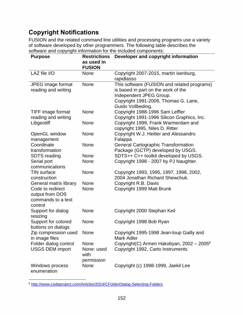
152

Copyright Notifications FUSION and the related command line utilities and processing programs use a variety of software developed by other programmers. The following table describes the software and copyright information for the included components:

Purpose Restrictions as used in FUSION

Developer and copyright information

LAZ file I/O None Copyright 2007-2015, martin isenburg, rapidlasso

JPEG image format reading and writing

None This software (FUSION and related programs) is based in part on the work of the Independent JPEG Group. Copyright 1991-2009, Thomas G. Lane, Guido Vollbeding.

TIFF image format reading and writing

None Copyright 1988-1996 Sam Leffler Copyright 1991-1996 Silicon Graphics, Inc.

Libgeotiff None Copyright 1999, Frank Warmerdam and copyright 1995, Niles D. Ritter

OpenGL window management

None Copyright W.J. Heitler and Alessandro Falappa

Coordinate transformation

None General Cartographic Transformation Package (GCTP) developed by USGS.

SDTS reading None SDTS++ C++ toolkit developed by USGS. Serial port communications

None Copyright 1998 - 2007 by PJ Naughter.

TIN surface construction

None Copyright 1993, 1995, 1997, 1998, 2002, 2004 Jonathan Richard Shewchuk.

General matrix library None Copyright R.B. Davis Code to redirect output from DOS commands to a text control

None Copyright 1999 Matt Brunk

Support for dialog resizing

None Copyright 2000 Stephan Keil

Support for colored buttons on dialogs

None Copyright 1998 Bob Ryan

Zip compression used in image files

None Copyright 1995-1998 Jean-loup Gailly and Mark Adler

Folder dialog control None Copyright(C) Armen Hakobyan, 2002 – 20056 USGS DEM import None: used

with permission

Copyright 1992, Carto Instruments

Windows process enumeration

None Copyright (c) 1998-1999, Jaekil Lee

6 http://www.codeproject.com/Articles/2024/CFolderDialog-Selecting-Folders

http://www.codeproject.com/Articles/2024/CFolderDialog-Selecting-Folders

153

Command line parsing logic

Unknown Copyright 1999-2003 Santronics Software, Inc.

Acknowledgements The FUSION software has been used by many people around the world. Some use the software in complete anonymity but others provide feedback and ask questions. In almost all cases, this feedback results in improvements or modifications to the software. I would like to personally thank fellow Forest Service researchers Steve Reutebuch and Hans-Erik Andersen for the endless hours of discussion and suggestions regarding the processing LIDAR data to produce useful information. Graduate students at the University of Washington, all of whom have moved on in their own careers, Yuzhen Li, Sooyoung Kim, Tobey Clarkin, and Jacob Strunk served as unofficial testers and helped to uncover lots of bugs during FUSION’s early development. Dr. Van Kane, also at the University of Washington, has processed more LIDAR data than most and his observations and suggestions have greatly improved the software and documentation. His focus on deriving ecologically important information from LIDAR point clouds and the subsequent enhancements and additions to FUSION will benefit all users of the software. I also want to thank Gordon W. Frazer, post-doctoral fellow in the Forest Geomatics Group at the Pacific Forestry Centre, Canadian Forest Service, in Victoria, British Columbia for suggesting the addition of L-moments and L-moment ratios to the suite of metrics computed by CloudMetrics and GridMetrics. These metrics have proved useful for a variety of applications. FUSION would not be successful without the training materials and first-line support provided by the Forest Service’s Remote Sensing Application Center (RSAC). The folks at RSAC provide support for anyone wanting to use FUSION or LiDAR. In particular, Denise Laes and Brent Mitchell developed the original tutorials. While Denise has moved on to another job, her diligence and organization while testing and developing workflows made FUSION a better product. Brent has taught FUSION and general LiDAR analysis to over 1800 people including groups in Mexico, Brazil, and the Philippines. The FUSION/LiDAR helpdesk maintained by RSAC fields questions from all over the United States. Finally I want to thank Martin Isenburg for all the work he has done to promote LIDAR data standards and develop the LAStools package. His efforts have benefitted all who work with both airborne and terrestrial scanner data. FUSION relies on his LASzip.dll to support the compressed point data files stored in his LAZ format. In addition, LAStools provides many capabilities that are not available in FUSION. Martin’s tools allow users to directly manipulate LAS data and his ground filtering and surface generation tools help users without ground surface models fully realize the potential of their data.

154

References Andersen, H.-E., R.J. McGaughey, and S.E. Reutebuch. 2005. Estimating forest canopy fuel parameters using LIDAR data. Remote Sensing of Environment 94(4):441-449. Baltsavias, E. P. 1999. Airborne laser scanning: basic relations and formulas. ISPRS Journal of Photogrammetry and Remote Sensing, 54(2-3): 199–214. Brandtberg, T. 2007. Classifying individual tree species under leaf-off and leaf-on conditions using airborne lidar. ISPRS Journal of Photogrammetry and Remote Sensing, 61(5): 325–340. Brennan, R. and Webster, T.L. 2006. Object-oriented land cover classification of lidar-derived surfaces. Canadian Journal of Remote Sensing, 32(2):162-172. Charaniya, A.P., Manduchi, R., and Lodha, S.K. 2004. Supervised parametric classification of aerial LIDAR data. In, CVPRW’04, Proceedings of the IEEE 2004 Conference on Computer Vision and Pattern Recognition Workshop, June 27 – July 2, 2004, Baltimore, Md. Vol. 3, pp. 1-8. Flood, M. 2001. LIDAR activities and research priorities in the commercial sector. International Archives of Photogrammerty and Remote Sensing, Vol. XXXIV Part 3/W4, Annapolis, MD, pp. 3-7. Hasegawa, H. 2006. Evaluations of LIDAR reflectance amplitude sensitivity towards land cover conditions. Bulletin of the Geographical Survey Institute, 53:43-50. Hosking, J.R.M. 1990. L-moments: analysis and estimation of distributions using linear combinations of order statistics. Journal of the Royal Statistical Society. Series B (Methodological). 52(1):105-124. Hug, C. and Wehr, A. 1997. Detecting and identifying topographic objects in imaging laser altimeter data. International Archives of Photogrammetry and Remote Sensing, Vol. XXXII Part 3-4/W2, Stuttgart, Germany, pp. 19-26. Hyyppä, J., Hyyppä, H., Litkey, P., Yu, X., Haggrén, X. H., Ronnholm, P., Pyysalo, U., Pitkänen, J., Maltamo, M. 2004. Algorithms and methods of airborne laser scanning for forest measurements. International Archives of Photogrammetry and Remote Sensing, Vol. XXXVI Part 8/W2, Freiburg, Germany, pp. 82-89. Jenness, J. 2006. Topographic Position Index (tpi_jen.avx) extension for ArcView 3.x, v. 1.2. Jenness Enterprises. Available at: http://www.jennessent.com/arcview/tpi.htm. Keating, Kim A.; Gogan, Peter J.P.; Vore, John M.; Irby, Lynn R. 2007. A simple solar radiation index for wildlife habitat studies. Journal of wildlife management 71(4):1344-1348.

http://www.jennessent.com/arcview/tpi.htm

155

Kini, A.U.; Popescu, S.C. 2004. TreeVaw: A versatile tool for analyzing forest canopy Lidar data – a preview with an eye towards future. Kansas City, MO: SPRS Images to Decision: Remote Sensing Foundation for GIS Applications. Kraus, K., and N. Pfeifer. 1998. Determination of terrain models in wooded areas with airborne laser scanner data. ISPRS Journal of Photogrammetry and Remote Sensing. 53: 193-203. McGaughey, R.J., Reutebuch, S.E., Andersen, H.-E. 2007. Creation and use of lidar intensity images for natural resource applications. In: 21st Biennial Workshop on Aerial Photography, Videography, and High Resolution Digital Imagery for Resource Assessment, May 15-17, 2007, Terre Haute, Indiana. ASPRS, Bethesda, MD. Unpaginated CD-ROM. Popescu, S.C., R.H. Wynne, and R.F. Nelson, 2002. Estimating plot-level tree heights with lidar: local filtering with a canopy-height based variable window size, Computers and Electronics in Agriculture, 37(1-3):71-95 Popescu, S.C., and R.H. Wynne, 2004. Seeing the trees in the Forest: Using Lidar and Multispectral Data Fusion with Local Filtering and Variable Window Size for Estimating Tree Height, Photogrammteric Engineering & Remote Sensing, Vol. 70, No. 5, May 2004, pp. 589-604. Silverman, B. W. 1986. Density Estimation. London: Chapman and Hall. Song, J.-H., Han, S.-H., Yu, K., and Kim, Y.-I. 2002. Assessing the possibility of land-cover classification using LIDAR intensity data, International Archives of Photogrammetry and Remote Sensing, Graz, Austria, 2002, Vol. XXXIV, Part 3B, pp. 259-262. Vincent, L and Soille, P. 1991. Watersheds in digital spaces: an efficient algorithm based on immersion simulations, IEEE Transactions on Pattern Analysis and Machine Intelligence, Vol. 13, No. 6, pp. 583-598. Weiss, A.D. 2001. Topographic position and landforms analysis. Poster Presentation, ESRI Users Conference, San Diego, CA (2001). Wang, O.J. 1996. Direct sample estimators of L moments. Water Resources Research. 32(12):3617-3619. Wehr, A. and Lohr, U. 1999. Airborne laser scanning—an introduction and overview. ISPRS Journal of Photogrammetry and Remote Sensing, 54:68–82. Woo, M., Neider, J, Davis, T. 1997. OpenGL programming guide: the official guide to learning OpenGL, version 1.1. Addison-Wesley.

156

Zevenbergen, Lyle W.; Thorne, Colin R. 1987. Quantitative analysis of land surface topography. Earth surface processes and landforms, 12:47-56.

157

Appendix A: File Formats

158

PLANS Surface Models (.DTM)

The Preliminary Logging Analysis System (PLANS) is a cable logging analysis system developed by the US Forest Service, Pacific Northwest Research Station in the early 1990’s. PLANS uses a binary format for its digital terrain models (DTM). The binary format offers several advantages over an ASCII format used in the early releases of PLANS:

1. A model stored in binary format, using two-byte Z-values, requires approximately 60 percent less storage space than the ASCII equivalent.

2. The binary format can be read faster than the ASCII format. Tests conducted in

1992 indicated the time required to read an entire model was about 50 percent less using the binary format.

3. Using the binary format it is possible to consistently calculate the byte position of

the elevation for a specific grid point in the model file. Using the ASCII format, which is flexible in the position of elevation values within the model file, it can be difficult (if not impossible) to consistently calculate the byte position of a given elevation. This allows PLANS programs to utilize the model without actually loading the entire model into memory. This final advantage becomes important when working with larger models that cannot be loaded into memory. Using the binary format, programs can use any size model as only small portions of the model are loaded into memory at any given time.

The binary format is relatively simple and contains the same information as the ASCII format. Additional descriptive parameters are included to facilitate DTM file management and future enhancements to PLANS, e.g., the ability to use non-integer elevations and the use of metric units (implemented 7/2002). When reading a PLANS DTM, it is tempting to define a structure for the header variables and then read the header as a block. Unfortunately, this approach often fails due to packing of structures by many compilers. To ensure a successful read, read the variables in the header one at a time.

Byte Offset Type Description

0-20 String *21 ASCIIZ terminated (chr$(0)) file signature for a PLANS DTM…must be "PLANS-PC BINARY .DTM" (20 characters long plus chr$(0)).

21-81 String *61 ASCIIZ terminated DTM name...entered by user to facilitate DTM file management. The DTM name will always be expanded with spaces to be 60 bytes long then the chr$(0) will be added.

82-85 Real*4 DTM file format version identifier: Original binary format (version 1.0): 3/7/90 Extended format (version 2.0): 1998 Modified to support all elevation storage types

159

(version 3.0): 7/2002 Added horizontal and vertical datum to header (version 3.1): 6/1/2005

86-93 Real*8 Lower left corner X-coordinate of the DTM area.

94-101 Real*8 Lower left corner Y-coordinate of the DTM area.

102-109 Real*8 Minimum Z-coordinate in the DTM.

110-117 Real*8 Maximum Z-coordinate in the DTM.

118-125 Real*8 Rotation of the DTM area within the coordinate system in radians. All versions: NO ROTATION IS ALLOWED.

126-133 Real*8 Spacing between columns in the DTM.

134-141 Real*8 Spacing between points along a column in the DTM.

142-145 Integer * 4 Number of columns in the DTM.

146-149 Integer * 4 Number of points in each column of the DTM.

150-151 Integer * 2 Flag indicating the units used for the DTM's lower left corner and the row and column spacing. 0 Feet 1 Meters 2 Other

152-153 Flag indicating the units used for the DTM's Z-coordinates. 0 Feet 1 Meters 2 Other

154-155 Integer * 2 Flag indicating the variable type used for Z-coordinate storage in the DTM file. 0 2-byte integer 1 4-byte integer 2 4-byte real number 3 8-byte real number 3/30/1990 ONLY TYPE 0 IS ALLOWED IN VERSION 1.0 and 2.0 FILES. 7/2002 Version 3.0 and newer supports all variable types

156-157 Integer * 2 Flag indicating the coordinate system for planimetric values.

0 Unknown (for compatibility with format 1.0 models) 1 UTM 2 State plane 3 Unknown 3+ Undefined…do not use values greater than 3 Format 2.0 and newer.

158-159 Integer * 2 Coordinate zone.

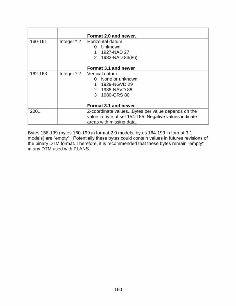
160

Format 2.0 and newer.

160-161 Integer * 2 Horizontal datum 0 Unknown 1 1927-NAD 27 2 1983-NAD 83(86) Format 3.1 and newer

162-163 Integer * 2 Vertical datum 0 None or unknown 1 1929-NGVD 29 2 1988-NAVD 88 3 1980-GRS 80 Format 3.1 and newer

200... Z-coordinate values...Bytes per value depends on the value in byte offset 154-155. Negative values indicate areas with missing data.

Bytes 156-199 (bytes 160-199 in format 2.0 models, bytes 164-199 in format 3.1 models) are "empty”. Potentially these bytes could contain values in futures revisions of the binary DTM format. Therefore, it is recommended that these bytes remain "empty" in any DTM used with PLANS.

161

LIDAR Data Files (.LDA)

The LDA format was developed as an alternative to ASCII text files commonly delivered by LIDAR providers. LDA files are binary and provide a moderately compact storage format. The advantage of the LDA format when compared to ASCII text files is that return data can be read randomly rather than serially (sequentially). When combined with the FUSION indexing scheme, the format allows efficient extraction of data samples. As of version 3.00 of FUSION, most utility programs write data in LAS format when input data are also in LAS format. This allows you to mix FUSION tools with other tools to analyze your data. After version 3.00, the LDA format will continue to be recognized by all programs. LDA files consist of a header and data records. The header is always 16 bytes long and contains the following items:


0-8 char *8 File signature used to identify the format. This field must contain the string “LIDARBIN”.

9-12 int * 4 Major version identifier.

13-16 int * 4 Minor version identifier.

The file version is formed using the following formula (C code):

Version = (float) major + (float) minor / 10.0f

Each point record is 36 bytes long and contains the following items:


0-3 int * 4 Pulse number.

4-7 int * 4 Return number.

8-15 real * 8 Easting (X).

16-23 real * 8 Northing (Y).

24-27 real * 4 Elevation.

28-31 real * 4 Nadir angle (or scan angle if not adjusted for aircraft attitude).

32-35 real * 4 Intensity.

When reading or writing LDA files from either C or C++, you must instruct the compiler to align structures on 4-byte boundaries if you want to read an entire point record into a structure.

162

Data Index Files (.LDX and .LDI)

The indexing scheme used by FUSION is simple and can be applied to all data files recognized by FUSION including the LDA format, LAS format, and ASCII text files. Indexing does not require modifications to the original data files. The indexing procedure first scans a LIDAR data file to determine the extent of the data coverage. The area is then overlaid with a 256 by 256 grid. A new file, called the index, is created containing one record for each LIDAR return in the source file. The record contains the column and row for the cell containing the data point and an offset into the raw data file to the start of the point record. After completing the index, it is sorted using the column and row values and a second file, called the first point file, is created listing the offset into the index file to the start of the first index entry for each cell in the index grid. Using the index and first point file, we can quickly locate and read all data points contained in a specific cell in the index grid. When extracting a data sample, FUSION determines the grid cells that potentially contain points in the sample and only reads data from these cells. The index file and the first point file use the same header record format. The header contains a checksum value that is computed from the data file modification time to help identify situations where a data file has been changed since it was indexed and, thus, should be re-indexed before use. The header contains the following items:


0-11 char * 12 File signature used to identify the format. This field must contain the string “LDAindex”.

12-15 real * 4 Version identifier.

16-19 int * 4 Checksum that will be compared to a checksum computed from the data file modification data and time to see if the data file has changed since the index was created.

20-23 int * 4 Format identifier for the data file. Format values are: 1 ASCII data 2 Binary LDA data 3 LAS data

23-30 real * 8 Minimum X value for the data.

31-38 real * 8 Minimum Y value for the data.

39-46 real * 8 Minimum Z (elevation) value for the data.

47-54 real * 8 Maximum X value for the data.

55-62 real * 8 Maximum Y value for the data.

63-70 real * 8 Maximum Z (elevation) value for the data.

70-73 int * 4 Number of grid cells in the X direction for the index grid. This value is usually 256.

74-77 int * 4 Number of grid cells in the Y direction for the index grid. This value is usually 256.

78-81 int * 4 Total number of points in the data file.

163

82-127 char * 46 Empty space. These byte locations can contain any value in index file versions 1.1 and older. Future version of the index files may use these bytes for additional data.

When reading or writing index files from either C or C++, you must instruct the compiler to align structures on 2-byte boundaries if you want to read an entire header record into a structure. For index files, the remainder of the file contains one record for each data point in the data file. The records contain the following items:


0-1 char * 1 Grid row containing the point.

2-3 char * 1 Grid column containing the point.

3-7 int * 4 Offset, in bytes, from the beginning of the data file to the start for the data for the point.

The records are stored in sorted order based on the column and row values (ascending). The origin of the column/row numbering scheme uses (0, 0) for the lower left corner. For the first point files the remainder of the file contains one value for each grid cell in the data index. The value represents the offset (int * 4) from the beginning of the index file to the first point in each cell. Offsets are stored by columns starting with the leftmost column and by row starting at the bottom of the column. The first value is the offset to first point in the lower left cell. The second value is the offset to the first point in the second row (from the bottom) of the leftmost column.

164

LAS LIDAR Data Files (.LAS)

The following description was taken from https://www.asprs.org/committee-general/laser-las-file-format-exchange-activities.html (last accessed 8/2016):

The LAS file format is a public file format for the interchange of LIDAR data between vendors and customers. This binary file format is a alternative to proprietary systems or a generic ASCII file interchange system used by many companies. The problem with proprietary systems is obvious in that data cannot be easily taken from one system to another. There are two major problems with the ASCII file interchange. The first problem is performance because the reading and interpretation of ASCII elevation data can be very slow and the file size can be extremely large, even for small amounts of data. The second problem is that all information specific to the LIDAR data is lost. The LAS file format is a binary file format that maintains information specific to the LIDAR nature of the data while not being overly complex.

FUSION reads version 1.0, 1.1, 1.2, 1.3, and some variants of version 1.4 LAS files as defined in the LAS format specification maintained on the web site listed above. When working with data stored in LAS format, FUSION writes LAS files that are fully compliant with the LAS specification. FUSION attempts to output data in the same version of the LAS format as the input data files. In cases where input data are stored in multiple LAS formats, FUSION will produce LAS outputs in the format that matches the lowest input LAS format version. When working with input data stored in ASCII text format, FUSION will produce LAS output files that, while they can be read by most other programs that read LAS format, are not complete. Some of the fields for each return are not populated. Specifically the field that details the number of returns for a pulse is always set to 0. This information would allow you to determine that a particular return is, for example, return 2 of 3 for the pulse. In addition, FUSION will produce LAS files for data that is missing items such as the GPS time, scan angle, and intensity.

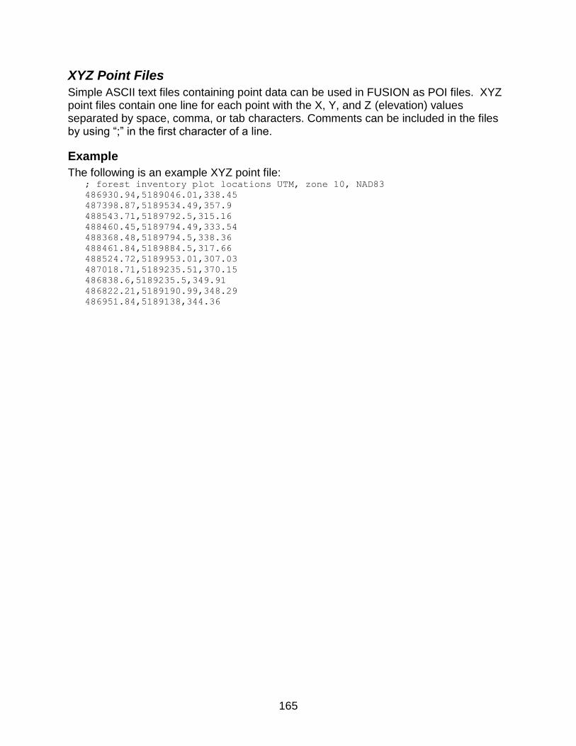
https://www.asprs.org/committee-general/laser-las-file-format-exchange-activities.html

https://www.asprs.org/committee-general/laser-las-file-format-exchange-activities.html

165

XYZ Point Files

Simple ASCII text files containing point data can be used in FUSION as POI files. XYZ point files contain one line for each point with the X, Y, and Z (elevation) values separated by space, comma, or tab characters. Comments can be included in the files by using “;” in the first character of a line.

Example

The following is an example XYZ point file: ; forest inventory plot locations UTM, zone 10, NAD83

486930.94,5189046.01,338.45

487398.87,5189534.49,357.9

488543.71,5189792.5,315.16

488460.45,5189794.49,333.54

488368.48,5189794.5,338.36

488461.84,5189884.5,317.66

488524.72,5189953.01,307.03

487018.71,5189235.51,370.15

486838.6,5189235.5,349.91

486822.21,5189190.99,348.29

486951.84,5189138,344.36

166

Hotspot Files

Hotspots are used to define specific locations that are liked to some action. Possible actions include loading a pre-defined data set, displaying an image file, running an external program, or just about anything else. Hotspot implementation in FUSION is similar to a link on a web page. You move the mouse over the hotspot, the cursor changes to a hand, and the information about the hotspot is displayed in the status display at the bottom of the FUSION window. Hotspot files are ASCII text files. They usually have an .HST extension. Each record (line) of the file defines a single hotspot. Lines starting with “#” or “;” in the first character position are treated as comments. The fields that define the hotspot are listed below in the order they should appear in the hotspot file. Field name Data type Description Minimum X Number Minimum X value that defines the hotspot

area. For icon hotspots, the minimum X and maximum X can be the same.

Minimum Y Number Minimum Y value that defines the hotspot area. For icon hotspots, the minimum Y and maximum Y can be the same.

Maximum X Number Maximum X value that defines the hotspot area.

Maximum Y Number Maximum Y value that defines the hotspot area.

Shape code Integer Code identifying the shape or type for the hotspot. Valid codes are:

4 rectangle 5 circle

100 icon:

101 icon:

102 icon:

103 icon:

104 icon:

105 icon:

106 icon:

107 icon:

167

108 icon:

109 icon: Action code Integer The action that FUSION should take

when the user selects a hotspot. Valid action codes are:

0 open the target object for viewing using the Windows application associated with the object type

1 display the target object using the old Scatter3D 3D visualization program

2 display the target object using the prototype 3DV visualization program

3 display the target object using the LDV 3D visualization program

99 treat the target object as a valid windows/DOS command line and execute the command using the WinExec function

Descriptive message

Quote-delimited string

Message that will be displayed on the status line along the bottom of the FUSION window. The actual message will be formed by concatenating the descriptive message and the command target.

Command target Quote-delimited string

The target object for the action code. In the case of Windows/DOS commands, the command target is use as-is with the WinExec function.

Examples

The following is a hotspot file that defines two types of hotspots. The first display the bullseye icon (type 101) and link to a pre-defined data set for LDV. The second set displays the information icon (type 100) and use a DOS command line to display an image file using the VIEWPIC program (VIEWPIC is distributed with FUSION and can display many image formats). For both types of hotspots, the same point could have been used for the minimum and maximum XY because icons do not rely on the hotspot area specified in the hotspot file but rather use a 32-pixel square area centered on the average of the minimum and maximum X and Y values to define the selection area.

168

; pre-defined LDV data files

976079.8661 567461.4061 976288.5761 567670.1161 101 3 "Display 1-acre data file containing blowdown using LDV: " "blowdown.set"

975383.5783 567601.0277 975800.9983 568018.4477 101 3 "Display 4-acre block from control unit using LDV: " "control4.set"

977367.9156 567913.5081 977733.9946 568279.5871 101 3 "Display 3-acre block for layer display using LDV: " "layers.set"

974776.5375 566912.6891 976503.1621 566942.6891 101 3 "Display 1727 by 30 ft corridor using LDV: " "corridor.set"

; treatment area images

975400 568100 975500 568200 100 99 "Display image showing conditions in control unit: " "viewpic control.jpg"

;975400 568100 975500 568200 100 99 "Display image showing conditions in control unit: " "viewpic images.lst"

976700 567100 976800 567200 100 99 "Display image showing conditions in 2-age unit: " "viewpic 2a.jpg"

976800 568200 976900 568300 100 99 "Display image showing conditions in clearcut unit: " "viewpic cc.jpg"

974300 566400 974400 566500 100 99 "Display image showing conditions in lightly thinned unit: " "viewpic lt.jpg"

169

Tree Files

Tree data files contain data representing the size and location of individual trees. Such data are usually measured in the field but analysis tools in the LIDAR Data Viewer (LDA) can output files of individual tree parameters extracted from LIDAR data. In FUSION, tree data are displayed like other point data except that the size of the point marker (except single pixels) is scaled to match the average width of the tree crown. When extracting samples, tree data can optionally be included in the sample. Tree data are used in LDV to display wire frame tree models consisting of a stem and a crown. Optional data specifying the color used when drawing the tree crown can be specified for each tree. This allows you to differentiate between species or condition classes when viewing the trees in LDV. Tree data are stored in CSV (comma separated values) format for compatibility with spreadsheet and database programs. The first line of the file contains column headings and subsequent lines contain the parameters for each tree. The first line of the file is ignored when reading trees even if it contains a valid tree record. Data for the tree measurements should use the same units as you LIDAR data. All heights and crown diameters should use the same units. The following values are needed for each tree: Field name Data type Description Tree identifier Number Identifier for the tree. The identifier can be a number

of a label. If the tree identifier is a negative number, the tree crown is drawn in LDV using a cylinder with a rounded top. If the tree identifier is positive, the tree crown is drawn using a paraboloid (rounded cone).

X Number X coordinate for the tree. Y Number Y coordinate for the tree. Elevation Number Elevation at the tree base. If this is 0.0, the elevation

will be adjusted in FUSION using the current terrain model.

Height Number Total tree height. Height to crown base

Number Height to the crown base. Definition of the crown base varies depending on the application and field protocols.

Maximum crown diameter

Number Maximum crown diameter. If the maximum and minimum crown diameters are 0.0, crown diameter will be estimated as 16% if the total tree height.

Minimum crown diameter

Number Minimum crown diameter. If the maximum and minimum crown diameters are 0.0, crown diameter will be estimated as 16% if the total tree height.

170

Crown rotation Number Rotation of the crown (degrees azimuth) used to properly orient elliptical crowns. If crowns are circular, the rotation should be 0.0.

Red (optional) Number Red color component for the color used to represent the tree crown in LDV.

Green (optional) Number Green color component for the color used to represent the tree crown in LDV.

Blue (optional) Number Blue color component for the color used to represent the tree crown in LDV.

Example

The following is an example tree file without color data for individual trees: ID,X,Y,Elev,Height,Ht To Crown Base,Max Crown Dia,Min Crown Dia,Crown Rotation

1,976311.380200,566629.267600,0.000000,174.016312,0.000000,55.883287,55.883287,0.000000

2,976347.328300,566651.065800,0.000000,172.034225,83.689568,41.537985,41.537985,0.000000

-3,977218.112900,567075.240000,0.000000,172.856262,102.127383,46.984066,46.984066,0.000000

4,976410.159500,567050.810000,0.000000,165.341171,74.987727,45.400783,45.400783,0.000000

5,976255.164700,566605.805300,0.000000,170.129089,0.000000,49.816029,49.816029,0.000000

Notice that negative identifier in the third record will cause the crown for this tree to be draw using a rounded-top cylinder. All other tree crowns will be drawn as paraboloids. The following is an example tree file with color information for each tree: ID,X,Y,Elev,Height,Ht To Crown Base,Max Crown Dia,Min Crown Dia,Crown Rotation,Red,Green,Blue

1,976311.380200,566629.267600,0.000000,174.016312,0.000000,55.883287,55.883287,0.0,0,255,0

2,976347.328300,566651.065800,0.000000,172.034225,83.689568,41.537985,41.537985,0.0,0,255,0

3,977218.112900,567075.240000,0.000000,172.856262,102.127383,46.984066,46.984066,0.0,255,0,0

4,976410.159500,567050.810000,0.000000,165.341171,74.987727,45.400783,45.400783,0.0,0,255,0

5,976255.164700,566605.805300,0.000000,170.129089,0.000000,49.816029,49.816029,0.0,0,255,0

In this example, the tree represented by the third record will be drawn with a red crown and all other trees will be drawn with green crowns.

171

ASCII LIDAR Data File Formats FUSION can process a variety of ASCII file formats to convert them to its own LDA format and create the index files to allow rapid random access. In addition, the XYZConvert command line utility also converts data in specific formats to FUSION’s LDA format. The formats listed below are formats that we have encountered in data sets from several vendors. Additional formats may be added in the future. FUSION also offers a generic ASCII data parser that allows you to define the format on the fly and save the format definition for later use both within FUSION and using the ASCIIImport utility. Use of the generic ASCII data parser is preferred over one of the fixed format conversion options. However, some formats cannot be parsed correctly by the generic parser. Namely, formats that included duplication of returns with one return coded as return # of # and the duplicate coded to indicate that the return was also identified as a bare-earth return. ASCII file conversion functions are accessed using the “Utilities” button and the “Convert ASCII file to binary LDA” button. All ASCII formats consist of one record per return with data fields separated by commas, spaces, or tabs. In general, the separator doesn’t matter even if the format description indicates that a specific character is used to separate data values. All lines in a data file that start with “#” or “;” are considered comments and ignored.

Simple ASCII XYZ (format 0)

Each record contains X, Y, elevation, [scan angle]. The scan angle is optional (see the “Convert and index XYZ files” dialog, “Read scan/nadir angle from fourth column” checkbox).

Terrapoint data (format 1)

Each record contains GPS time, return number, Y, X, elevation, aircraft X, aircraft Y, aircraft elevation, and intensity.

AeroTec 1999 ASCII (format 2)

Each record contains pulse number, return number, X, Y, elevation, scan angle, and intensity separated by spaces

AeroTec 1998 ASCII (format 3)

Each record contains pulse number, Y, X, and elevation separated by spaces.

Aeromap CXYZI (format 4)

Each record contains return number, X, Y, elevation, and intensity separated by commas.

Aeromap XYZI (format 5) and Cyrax XYZI (format 6)

Each record contains X, Y, elevation, and intensity separated by commas.

172

Aeromap Kenai project (format 7)

Each record contains GPS time, X, Y, elevation, return number, intensity, nadir angle, and roll angle separated by commas.

Aeromap Kenai final ALL RETURNS (format 8)

Each record contains the GPS time, X, Y, Z, planeX, planeY, planeZ, class (return), intensity, scan angle, and a bare earth flag separated by commas. This format also includes a 14 line header that is ignored during the conversion process.

Aeromap Kenai final GROUND POINTS ONLY (format 9)

Each record contains the GPS time, X, Y, Z, planeX, planeY, planeZ, class (return), intensity, scan angle, and a bare earth flag separated by commas. Only points with the bare earth flag set to 1 are converted. This format also includes a 14 line header that is ignored during the conversion process.

Aeromap Kenai final FIRST RETURNS ONLY (format 10)

Each record contains the GPS time, X, Y, Z, planeX, planeY, planeZ, class (return), intensity, scan angle, and a bare earth flag separated by commas. Only points with class set to 1 are converted. This format also includes a 14 line header that is ignored during the conversion process.

Aeromap Kenai final LAST RETURNS ONLY (format 11)

Each record contains the GPS time, X, Y, Z, planeX, planeY, planeZ, class (return), intensity, scan angle, and a bare earth flag separated by commas. Only points that are the last return for the pulse are converted. Special logic is used to compare GPS times for returns and the class value to determine which return is the last return. This format also includes a 14 line header that is ignored during the conversion process.

Aeromap UW campus (format 12)

Each record contains the GPS time, X, Y, Z, return number, and intensity separated by commas. For these data, only returns 1 through 3 are valid returns. Return number 4 indicates that the return is a last return and it may or may be a duplicate of one of the other returns for the pulse. Return number 5 indicates that the return is a bare-earth point and is always a duplicate of one of the other returns.

Aeromap UW campus GROUND RETURNS ONLY7 (format 13)

Each record contains the GPS time, X, Y, Z, return number, and intensity separated by commas. Using this format in XYZConvert produces files that contain only the returns classified as bare-earth returns. For these data, only returns 1 through 3 are valid returns. Return number 4 indicates that the return is a last return and it may or may be a duplicate of one of the other returns for the pulse. Return number 5 indicates that the return is a bare-earth point and is always a duplicate of one of the other returns.

7 These format are only available in XYZConvert.

173

Puget Sound LIDAR Consortium 2003 data from Terrapoint7 (format 14)

Each record contains the GPS week, GPS second, X, Y, Z, # returns for pulse, Return #, Off-nadir angle, Intensity, and Return classification separated by commas. Interpretation of the Return number is as follows:

Return number in data

Interpretation

1-4 The return is return 1, 2, 3, or 4. 5 The return was a first return and also the

last return for the pulse (only one return was recorded for the pulse).

6 The return was the second return and also the last return for the pulse.

7 The return was the third return and also the last return for the pulse.

8 The return was the fourth return and also the last return for the pulse.

Return classification values are as follows:

Return classification

Interpretation

B Blunder (the returns should be ignored for must processing).

G The return is a bare-earth return. V The return represents vegetation. S The return represents a structure.

Puget Sound LIDAR Consortium 2003 data from Terrapoint LAST RETURNS ONLY7 (format 15)

Each record contains the GPS week, GPS second, X, Y, Z, # returns for pulse, Return #, Off-nadir angle, Intensity, and Return classification separated by commas. Using this format in XYZConvert produces files that contain only the last returns recorded for each pulse. Interpretation of the Return number and Return classification are the same as for the previous format.

Terrapoint data for Fort Lewis, WA7 (format 16)

Each record contains the Return name, X, Y, Elevation, and Intensity separated by commas.

Spectrum Mapping data for King County, WA7 (format 17)

Each record contains the X, Y, Z, Return number, and Number of returns for the pulse separated by commas.

174

PSLC 2004 data for Pierce County, WA (format 18)

Each record contains the GPS week, GPS second, X, Y, Z, Ellipsoid Ht, Nadir angle, and Return number separated by spaces.

PSLC 2000 data for Tiger Mountain area, WA (format 19)

Each record contains the X, Y, Z, Ell ipsoid ht, GPStime, Return #, Scan angle, ABS scan angle, and GPS week separated by commas.

175

Appendix B: DOS Batch Programming and the FUSION LIDAR Toolkit

176

Batch Programming Overview

In MS-DOS and Windows, a batch file is a text file containing a series of commands intended to be executed by the command interpreter. When a batch file is run, the shell program (usually COMMAND.COM or cmd.exe) reads the file and executes its commands, normally line-by-line. A batch file is analogous to a shell script in Unix-like operating systems. Batch files are useful for running a series of executables automatically. Many system administrators use them to automate tedious processes. Although batch files support elementary program flow commands such as IF and GOTO, they are not well-suited for general-purpose programming. DOS batch files have the filename extension .BAT and are normally executed from a command prompt window. To launch a command prompt window, go to “Start”, “Programs”, “Accessories” and select “Command Prompt”. An alternative method for launching a command prompt window is to go to “Start”, select Run…” and type “CMD” followed by [Enter]. Once the command prompt window is running, you can use DOS commands to manually accomplish various tasks. Use the HELP command to get help for additional DOS commands. To run a batch file from a command prompt, simply type the name of the batch file without the .BAT extension.

Getting help with batch programming commands

All versions of Windows

Open a command prompt window and type “help” followed by pressing [Enter]. This will display a list of all available batch file commands. You can also get information for specific commands by typing “help” followed by the command name.

Windows XP

Go to "Start", then "Help and Support", then under the Pick a Task" section, select the "Tools" link. At the very bottom of the Tools list, you'll find three entries that will help you with your command-line batch questions. The best thing there is the "Command-line reference A-Z". If you have an OEM version of Windows (Like Dell, where they replaced the Help section with something else), you may need to read the XP Command-line reference A-Z on the web.

Windows 2000

Go to "Start", then "Help", then click the “Contents” tab, then "Reference", then "MS-DOS Commands".

177

Using the FUSION Command Line Tools

The FUSION command line tools are used from a command prompt. The command prompt provides a low-level interface to your computer system. The command prompt in Windows 2000 and newer versions is similar to a DOS prompt. FUSION commands can be run from any folder by typing the full path to the program. This means you have to know the install directory for FUSION and type its folder name before the command name. For example to run the FUSION Catalog program, you would type the following:

c:\fusion_install\catalog

If the FUSION install folder name includes spaces, you need to enclose the folder and program name in quotation marks like this:

“c:\Program files\fusion\catalog”

Command line options go outside the quotation marks. Anytime you use a folder name that includes spaces as part of a file specification on a command line, you need to enclose the folder and file name in quotation marks. Typing the full path is acceptable for a few commands but it is much easier to add the FUSION install directory to the search path for your computer. Then you can type FUSION commands from any folder on your computer without the install folder name. This can be accomplished in a command prompt window or by modifying the system properties. From a command prompt, the following command adds the FUSION install directory “C:\FUSION” to the search path:

Path %PATH%;C:\FUSION

This will only affect the open command prompt window so it needs to be repeated each time a command prompt window is opened. For a system wide change that will be in effect whenever a command prompt is opened, you can modify the system properties as described on the following web site (the exact steps will vary depending on your operating system):

https://helpdeskgeek.com/windows-10/add-windows-path-environment-variable/ (last accessed April 2018)

You will need to edit the system variable named “path” and append a semi-colon and the full folder name for the FUSION install directory (without the final “\”).

For Windows 7 and newer, the command prompt must be run using administrator privileges to prevent warning messages each time a new command in executed from a batch file This can be accomplished by right clicking on the icon for cmd.exe in the Windows file explorer and selecting the “Run as administrator” option. If you cannot use this option or it is not available in the list of options, consult your system administrator for assistance.

https://helpdeskgeek.com/windows-10/add-windows-path-environment-variable/

178

Automating Processing Tasks

Perhaps the easiest way to automate batch processing is through the use of the DOS FOR statement to queue processing on a series of data files. To do this, you need to create two batch files and one list of files to process. The first batch file processes a single data file and the second queues the processing of a series of data files by calling the first batch file with different data file names. Development of the first batch file is relatively straight forward in that it is just like the commands you type at the command prompt. The only difference is that instead of typing a data file name, you use the command line substitution parameter, %1, to call the batch file to run with a file name passed from the second batch file. The second batch file uses the DOS FOR command and a separate text file that lists all of the data files to process. To illustrate, let’s try an example where we want to filter ground points from a series of data files and create gridded surface models using the ground points. The list of files to process contains the names of each data file. Such a list can be generated using the DOS DIR command as follows:

DIR /b *.las > filelist.txt

This command will produce a file named filelist.txt that contains all LAS data files in the current folder. For more information on the DIR command, type HELP DIR at the command prompt. The list file will also contain the extension for each file. In some cases, you want to use only the data file name to construct the name of output files. This can be accomplished two ways. First, you can edit the file list and delete the extensions from the file name. Second, you can use parameters in the DOS FOR command to read the filename but omit the extension. This example uses the second method. The list file should look something like this:

The first batch file, named process_tile.bat, processes an individual data file. Notice that the substitution variable, %1, has been used instead of explicit file names. This allows us to pass the data file name from the second batch file to the first. Also notice that we have to provide the extension for the data file (.las) as it will not be read from the list of file names. Process_tile.bat contains the following commands:

DA75_LI080204.las

DA76E1_LI080204.las

DB72E1_LI080204.las

DB73_LI080204.las

DB76_LI080204.las

DC71A5_LI080204.las

DC71_LI080204.las

groundfilter %1_ground_pts.lda 3.5 %1.las

gridsurfacecreate %1_ground.dtm 1 m m 1 10 2 2 %1_ground_pts.lda

179

The second batch file, named process.bat, reads the list of file names and calls the first batch file for each data file. Process.bat contains the following commands:

In the command above, notice that there is a space before the second quotation mark (after the first period). If the file names listed in filelist.txt contain spaces, the names will not be parsed correctly and the process_tile.bat file will not function as expected. To start the processing, make the directory containing the data files the current directory and simply type process at the command prompt. All of the files listed in filelist.txt will be processed and the outputs stored in the current directory. If you want to use different folders to better organize outputs, include the folder names in the file names specified for outputs in process_tile.bat.

Mixing FUSION processing with other software packages

FUSION tools can be called from a variety of analysis tools including Python, R, and PERL. FUSION tools can even be called from within GIS environments allowing you to conduct analyses and view outputs in a common environment. Such applications can be very powerful but there are some cautions when calling tools from within GIS environments. The biggest issue is that most GIS platforms, and tools like Excel, lock files for read and write access when they are displayed on screen or included in a workspace. This behavior will prevent other software, including FUSION tools, from opening the files and can lead to errors or behaviors that are hard to track down. If you are working in these environments, be sure that files you are using for your analyses are not open in any other software package.

for /F "eol=; tokens=1* delims=,. " %%i in (filelist.txt) do call process_tile %%i

180

Appendix C: Using LTKProcessor to Process Data for Large Acquisitions

181

Overview

LTKProcessor is designed to facilitate the application of FUSION-LTK tools to large data acquisitions. It uses multiple data files to create seamless data products covering the entire acquisition area. In operation, LTKProcessor allows you to process data tiles individually, clip new data tiles that optionally include a buffer around the tile, or overlay an analysis grid over the entire acquisition extent. LTKProcessor does not actually process data. Instead, it creates a batch file that directs the processing. This batch file can be run from within LTKProcessor or from a command prompt. While the batch file is running, additional programs (LTKStatusMessenger8 and LTKStatusMonitor) graphically show the status of the processing job. The batch file produced by LTKProcessor is modular and can be used to accomplish several processing tasks by simply replacing the commands used to process each data tile or analysis grid cell. In addition, the batch file includes simple error checking logic that can alert users when errors are encountered while processing specific data tiles. Users of LTKProcessor still have to write batch files to process a single tile of data but they do not have to worry about the details of subdividing the point cloud into manageable data tiles or developing the batch logic to direct the processing flow. When processing data using batch files generated by LTKProcessor, LTKStatusMonitor displays the status of all data tiles (Figure 9). Tiles are gray if they have not been processed, yellow if they are currently being processed, green if processing ended without errors, and red if processing ended with errors. You can click on a tile to display its name at the bottom of the LTKStatusMonitor window. Once a tile is selected, you can use the “Show tile status” button to display the processing log for the individual tile (provided the option in LTKProcessor was checked to maintain log files for individual tiles). In addition, the tile status dialog (Figure 10) shows the commands needed to reprocess a single tile or to restart the processing job beginning with the selected tile. When an individual tile fails, you can reprocess the individual tile and then run the post-processing commands.

Considerations for Processing Data from Large Acquisitions

LIDAR systems produce large quantities of data—even for relatively small project areas. The sheer volume of the data makes it difficult to copy data sets and can lead to problems when processing data to provide information products from the point clouds. Limitations of computer operating systems can further complicate processing. The following sections discuss some of the issues that should be considered when planning the processing of data from LIDAR acquisitions. These discussions are based on experience processing data from several acquisitions ranging in size from 30,000 to 250,000 acres and containing up to 20 billion points. For the most part, FUSION and the LTK toolkit are designed to operate with large data sets. However, careful planning can ensure that processing is accomplished efficiently and reduce the chance for errors related to file sizes or computer memory limitations.

8 The LTKStatusMessenger program was called LTKStatusUpdate in FUSION versions prior to 3.60. The name was changed to allow the use of the program without administrator rights.

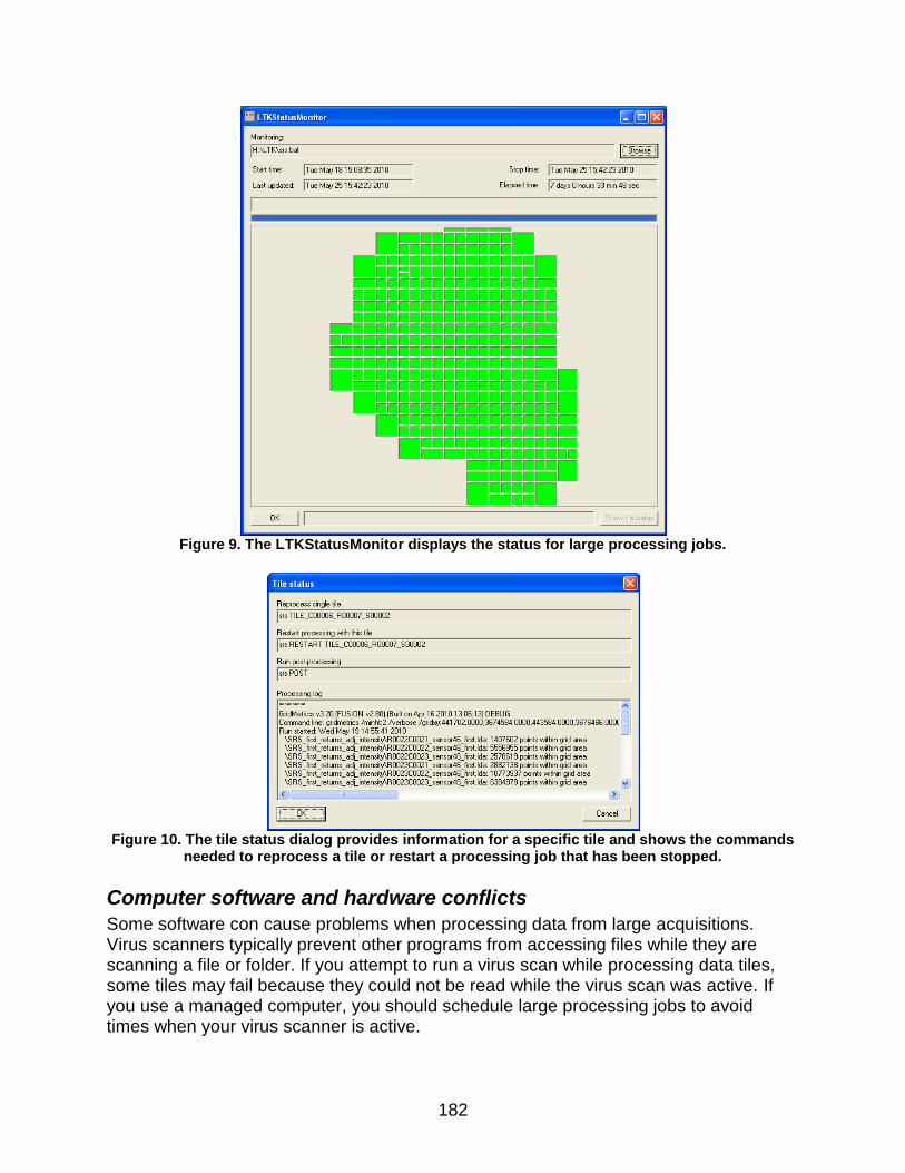
182

Figure 9. The LTKStatusMonitor displays the status for large processing jobs.

Figure 10. The tile status dialog provides information for a specific tile and shows the commands

needed to reprocess a tile or restart a processing job that has been stopped.

Computer software and hardware conflicts

Some software con cause problems when processing data from large acquisitions. Virus scanners typically prevent other programs from accessing files while they are scanning a file or folder. If you attempt to run a virus scan while processing data tiles, some tiles may fail because they could not be read while the virus scan was active. If you use a managed computer, you should schedule large processing jobs to avoid times when your virus scanner is active.

183

If you have LIDAR data stored on network attached storage devices and other people or computers are working on the same files, access to a tile may be blocked. Most LTK programs open files in read-only modes. However, other software may completely lock the files so no other applications can access the files. For output files in CSV format, you cannot have the file open in MS Excel while you are trying to read or write the file in any LTK program. This is a common problem when using CloudMetrics to compute metrics for a series of files. The typical scenario is that you are experimenting with options for CloudMetrics and then viewing the output (a CSV file) in Excel. You forget to close the file in Excel and then run CloudMetrics and find that the file was not updated and you get an error in CloudMetrics. The solution is to make sure that you don’t have the CSV file open in Excel before running a tool that will write to the open file. This is not a problem if you are using Notepad or Wordpad to view a file.

Pulse density and tile size

Pulse density (and therefore return density) is relatively uniform during a LIDAR acquisition. The flight pattern, aircraft speed, and scanner setting are all adjusted to obtain a desired pulse density. However, when the final data are assembled, it is not uncommon to have areas with pulse densities higher or lower than planned. As data are packaged for delivery, a tiling scheme is used to organize the data into blocks that provide a compromise between the size of each file and the number of files that must be managed. For areas covered by “extra” flight lines, the pulse density within a single tile may be double that of other tiles. Such areas result when a flight line is re-flown or when lines perpendicular to the bulk of the lines are flown to assist in relative error assessment and minimization. Processing workflows that are designed with the “normal” pulse density as an input may run into problems when they encounter a tile with twice as many pulses. FUSION and the LTK toolkit were designed using a simple philosophy. It was assumed that all the points contained in a single file and needed for any analyses could be held in memory for processing. While this basic assumption greatly simplified development efforts, it does not necessarily result in the most efficient processing. In general, all of the LTK tools can process at least 30 million data points in a single block on a computer with 1Gb of available memory (available when the program is invoked not simply the amount of memory installed in the computer). However, some tools can handle more points. As a general rule, processing is much more efficient when the data for an acquisition can be divided into as few tiles as possible. This is especially true when data are read from external hard drives where the time required to read the data is a significant portion of the overall processing time. Internal hard drives (or possibly external drives using the eSATA interface) tend to be much faster when reading large files. LTKProcessor provides several options to help “re-tile” data to make processing more efficient. These options are discussed in Subdividing large datasets.

Tile buffering

The ideal processing situation is when all data for a project can be loaded into memory and processed in a single step. However, almost all LIDAR acquisitions are simply too large to process in such a manner. Data are delivered in “tiles”. The size of each tile is

184

usually a function of the point density but many projects simply subdivide standard 7.5-minute quadrangles into a manageable number of tiles. While this approach produces individual files that are generally smaller than 1 Gb, it presents special problems when deriving information products that must span several tiles. Processing workflows that process each tile independently often result in discontinuities along tile edges that become problematic when adjacent tiles are combined. To overcome these problems and produce information that is not affected by tiling arrangements, it is possible to add a buffer around each tile, process the data, and then clip the resulting products using the original tile boundary. In general the buffer is one or two “cells” wide and requires that return data from the eight tiles adjacent to each tile being processed are read. Many of the LTK tools offer the option to use a buffer around the analysis area to make processing results more consistent. LTKProcessor provides options to specify the buffer size and to ensure that the tiling grid and buffer size is arranged to produce tiles that are exact multiples of the analysis cell size

Acquisition area arrangement (single area or multiple areas in 1 delivery)

When LIDAR acquisition contracts include more than one project area, special care must be taken to make sure processing occurs for each of the areas independently. A single data delivery may include data for multiple geographic areas separate by large distances. Attempts to process all the data in one “pass” will result in output products that have large areas with invalid results since the outputs will be sized to an area defined by the overall data extent. The easiest way to organize the data is to arrange point files using a separate folder for each distinct project area. In addition, LTKProcessor provides an option to view the input data tile arrangement. This option allows you to make sure the data is geographically “connected”.

Available drive space

There is no denying that LIDAR acquisitions produce large data sets. Delivered data totaling over 200 Gb are not uncommon. Most LIDAR data are delivered on external hard drives as it is too time consuming to burn data to DVD or other media. As data are processed, additional storage space is required for intermediate and final products. As a general rule, you will need free storage space totally at least 25 percent of the space needed for the point data alone.

Directory structure for processing and LTK outputs

Everyone has their own system for organizing files on their computer. FUSION and the LTK toolkit do not expect or impose a directory (folder) structure. However, it is useful to consider the organization before you start processing a data set. I have found that it works well to have all of the data and processing outputs for a project stored in a single folder at the root level of the storage drive. This folder should contain sub-folders to help organize the data and outputs. This makes copying the data much easier and helps ensure that batch files will work when the data are copied to a different drive. In addition, I keep all batch files used for processing in a separate folder and all data products in a separate folder with sub-folders as needed to keep things organized. When developing batch files (scripts), I include as little of the directory path for input and output files in commands as possible and never include the drive letter in any

185

commands. For batch files, I assume that their execution will start in the folder containing all of the batch files. If the current folder needs to be changed, the change is handled by the batch files and the current folder is always set back to the folder that contains all the batch files when processing is complete. The overall goal for the file arrangement is to have the data and processing relationships be independent of the drive letter and the structure above the project folder.

Data storage device (internal versus external hard drive)

LIDAR data are typically delivered on external hard drives. While this media is very convenient and low cost, it is usually not the best choice for processing. External drives fail!! You should not rely on the drive delivered by the data provider as the only copy of your data. One simple strategy is to copy the data onto a second drive as soon as you receive it and put the original drive in a safe place. Then copy the data onto a fast drive (either a fast external drive, network drive, or an internal drive) for processing. For tasks that involve processing of all point data files, simply copying the data to an internal drive and then processing from the internal drive can reduce processing times significantly. As you develop batch files for processing data, you will find that a similar sequence of commands is used for each data acquisition—maybe even the same sequence. If you are careful when developing your batch files, they can be used for different projects with a minimum of changes. I find it useful to make backup copies of all batch files (on a different drive than the data). This way if something happens to the drive containing the data, I can quickly recover the data from the original hard drive (stored in a safe place), copy the processing batch files, and start reprocessing the data. Ideally, backup copies of derived layers should be made on a regular basis. At a minimum, creating backup copies of the batch files allows you to easily (not necessarily quickly) recreate derived layers.

Error detection and recovery

LTKProcessor and LTKStatusMonitor provide limited error detection. It is likely that this capability will be enhanced in future versions of LTKProcessor. The master batch file created by LTKProcessor includes logic to detect errors while processing individual tiles and LTKStatusMonitor will show the tiles affected by the error in red. However, this logic will detect errors from the last process run for each tile. If you include multiple commands in the tile batch file, only the return status from the last command will be used to detect an error. To overcome this limitation, the LTKERROR environment variable can be set to any non-zero value to indicate an error when processing an individual tile. Upon return from the tile batch file, this variable is checked in addition to the DOS ERRORLEVEL to see if any errors occurred. If multiple commands are used in the tile batch file, you should set the LTKERROR variable to indicate an error using the following code fragment:

186

For example, suppose we want to use GroundFilter to identify bare-ground returns in a data tile and then use GridSurfaceCreate to produce a gridded terrain model using the bare-ground points. The simple commands added to the tile batch file would look like this:

If this sequence of commands were added to the tile processing batch file, the master batch file would only detect errors that occurred in GridSurfaceCreate. If GroundFilter failed, the data tile would still be reported in LTKStatusMonitor as complete. To remedy this problem we could insert use the following command sequence:

This would allow the master batch file to detect errors in both programs. However, it is likely that we don’t want to run GridSurfaceCreate if GroundFilter fails so the best command sequence to use would look like this:

This command sequence only runs GridSurfaceCreate if GroundFilter is successful and still sets the LTKERROR variable to indicate that an error occurred just in case the tile batch file contains other statements.

rem command to do something

IF ERRORLEVEL set LTKERROR=1

rem command to do something


GroundFilter parameters…

GridSurfaceCreate parameters…






IF NOT ERRORLEVEL (



)

ELSE (

set LTKERROR=1

)

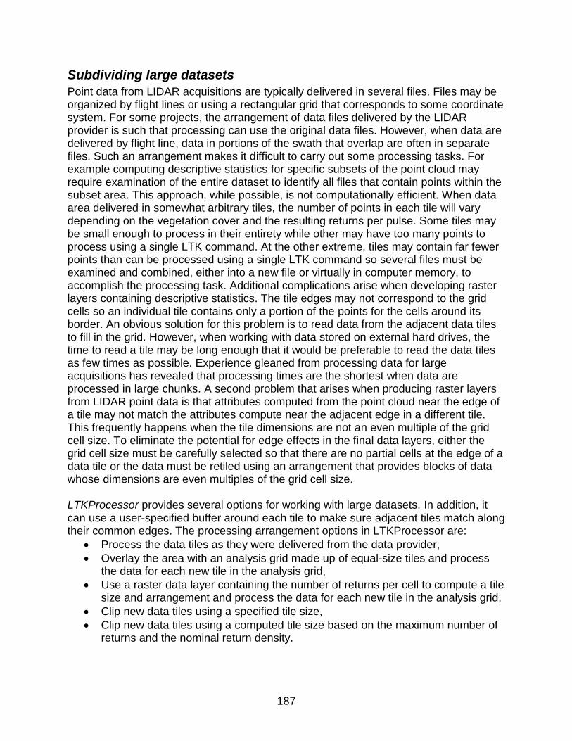
187

Subdividing large datasets

Point data from LIDAR acquisitions are typically delivered in several files. Files may be organized by flight lines or using a rectangular grid that corresponds to some coordinate system. For some projects, the arrangement of data files delivered by the LIDAR provider is such that processing can use the original data files. However, when data are delivered by flight line, data in portions of the swath that overlap are often in separate files. Such an arrangement makes it difficult to carry out some processing tasks. For example computing descriptive statistics for specific subsets of the point cloud may require examination of the entire dataset to identify all files that contain points within the subset area. This approach, while possible, is not computationally efficient. When data area delivered in somewhat arbitrary tiles, the number of points in each tile will vary depending on the vegetation cover and the resulting returns per pulse. Some tiles may be small enough to process in their entirety while other may have too many points to process using a single LTK command. At the other extreme, tiles may contain far fewer points than can be processed using a single LTK command so several files must be examined and combined, either into a new file or virtually in computer memory, to accomplish the processing task. Additional complications arise when developing raster layers containing descriptive statistics. The tile edges may not correspond to the grid cells so an individual tile contains only a portion of the points for the cells around its border. An obvious solution for this problem is to read data from the adjacent data tiles to fill in the grid. However, when working with data stored on external hard drives, the time to read a tile may be long enough that it would be preferable to read the data tiles as few times as possible. Experience gleaned from processing data for large acquisitions has revealed that processing times are the shortest when data are processed in large chunks. A second problem that arises when producing raster layers from LIDAR point data is that attributes computed from the point cloud near the edge of a tile may not match the attributes compute near the adjacent edge in a different tile. This frequently happens when the tile dimensions are not an even multiple of the grid cell size. To eliminate the potential for edge effects in the final data layers, either the grid cell size must be carefully selected so that there are no partial cells at the edge of a data tile or the data must be retiled using an arrangement that provides blocks of data whose dimensions are even multiples of the grid cell size. LTKProcessor provides several options for working with large datasets. In addition, it can use a user-specified buffer around each tile to make sure adjacent tiles match along their common edges. The processing arrangement options in LTKProcessor are:

Process the data tiles as they were delivered from the data provider,

Overlay the area with an analysis grid made up of equal-size tiles and process the data for each new tile in the analysis grid,

Use a raster data layer containing the number of returns per cell to compute a tile size and arrangement and process the data for each new tile in the analysis grid,

Clip new data tiles using a specified tile size,

Clip new data tiles using a computed tile size based on the maximum number of returns and the nominal return density.

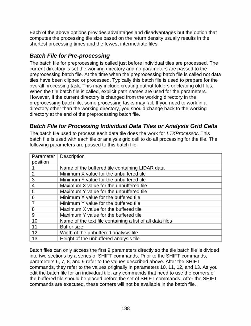
188

Each of the above options provides advantages and disadvantages but the option that computes the processing tile size based on the return density usually results in the shortest processing times and the fewest intermediate files.

Batch File for Pre-processing

The batch file for preprocessing is called just before individual tiles are processed. The current directory is set the working directory and no parameters are passed to the preprocessing batch file. At the time when the preprocessing batch file is called not data tiles have been clipped or processed. Typically this batch file is used to prepare for the overall processing task. This may include creating output folders or clearing old files. When the tile batch file is called, explicit path names are used for the parameters. However, if the current directory is changed from the working directory in the preprocessing batch file, some processing tasks may fail. If you need to work in a directory other than the working directory, you should change back to the working directory at the end of the preprocessing batch file.

Batch File for Processing Individual Data Tiles or Analysis Grid Cells

The batch file used to process each data tile does the work for LTKProcessor. This batch file is used with each tile or analysis grid cell to do all processing for the tile. The following parameters are passed to this batch file:

Parameter position

Description

1 Name of the buffered tile containing LIDAR data

2 Minimum X value for the unbuffered tile

3 Minimum Y value for the unbuffered tile

4 Maximum X value for the unbuffered tile

5 Maximum Y value for the unbuffered tile

6 Minimum X value for the buffered tile

7 Minimum Y value for the buffered tile

8 Maximum X value for the buffered tile

9 Maximum Y value for the buffered tile

10 Name of the text file containing a list of all data files

11 Buffer size

12 Width of the unbuffered analysis tile

13 Height of the unbuffered analysis tile

Batch files can only access the first 9 parameters directly so the tile batch file is divided into two sections by a series of SHIFT commands. Prior to the SHIFT commands, parameters 6, 7, 8, and 9 refer to the values described above. After the SHIFT commands, they refer to the values originally in parameters 10, 11, 12, and 13. As you edit the batch file for an individual tile, any commands that need to use the corners of the buffered tile should be placed before the set of SHIFT commands. After the SHIFT commands are executed, these corners will not be available in the batch file.

189

The file name passed to the batch (parameter 1) file looks like this: TILE_C00001_R00002_S00001. The row and column numbers specify the tile location and the subtile designation identifies the tile within an analysis grid cell when tile sizes have been optimized. The origin of the row and column coordinate system is the lower left corner of the data extent. When developing this batch file, only commands that are needed for each data tile should be included. This batch file will be called for each data tile so any extra commands will slow the overall processing.

Batch File for Final Processing

The batch file for final processing is called after all tiles have been processed. If new data tiles were clipped and saved, they will be available to this batch file. Outputs created in the preprocessing batch file and the tile processing batch file will also be available. This batch file is typically used to combine outputs produced for each data tile and to convert the combined output into formats more useful to non-LTK applications. The final processing batch file can change the current directory if needed and does not need to change it back to the working directory.

Example Batch Files

The FUSION distribution includes example batch files for pre-processing, tile processing, and final processing. The examples present one way to approach processing for large acquisitions and are intended to help users get started using LTKProcessor. Use of LTKProcessor is required to create the over-arching runstream that calls the example batch files. Output from the example processing batch files includes a set of raster data layers containing elevation, intensity, and topographic metrics for point data. Additional outputs can include canopy surface and height models, metrics computed from the canopy height model, and metrics computed for various height strata. The example processing requires a bare-earth surface model in FUSION’s DTM format, point files, and a return density raster layer (created by the RUNQAQC.BAT batch file). It is possible to modify the TILE.BAT file to create a bare-earth surface model for each processing tile but this is not the ideal processing flow since processing tiles can vary in size and the resulting bare-earth surface model may not work well for all processing tasks. The pre-processing batch file is named SETUP.BAT. It includes environment variable definitions that specify parameters to control most processing tasks and commands to create a directory structure for FUSION outputs. Variables are included that control creation of canopy surface and canopy height models and whether or not metrics are computed for elevation/height strata. Typical modifications to SETUP.BAT to customize it for a specific situation include changing the HOMEFOLDER, DTMSPEC, UNITS, CELLSIZE, LATITUDE, HTCUTOFF, COVERCUTOFF, COORDINFO, and OUTLIER variables. You can control computation of the canopy surface and strata metrics by changing the DOCANOPY and DOSTRATA variables. The CANOPYSTATSFILEIDENTIFIER variable must be changed to reflect the cell size for the canopy surface metrics.

190

The tile processing batch file, named TILE.BAT, creates canopy height and surface models for each analysis tile and computes metrics for the point data. It uses the CanopyModel, GridSurfaceStats, ClipDtm, and GridMetrics programs with parameters specified in SETUP.BAT. The example file assumes that bare-earth surface models already exist and have been converted in to FUSION’s DTM format. If this is not the case, you can use a call to GroundFilter to identify bare-earth points and then call GridSurfaceCreate to create a surface file. You will also need to change commands that use the bare-earth surface model (CanopyModel and GridMetrics). The post-processing batch file, named BUILDLAYERS.BAT, extracts individual point-cloud metrics from the GridMetrics outputs and merges the results for all analysis tiles into a single raster layer for each metric. In addition, this batch file merges canopy height and surface models and canopy metrics into individual raster layers. The example BUILDLAYERS.BAT extracts all of the metrics computed by GridMetrics and GridSurfaceStats. If you do not require all of the metrics, make changes to BUILDLAYERS.BAT to extract only the metrics you require. The RUNQAQC.BAT batch file is designed to be run before any LTKProcessor activity. It creates a basic QA report for the data acquisition and, most importantly, creates a return density raster layer that is used in LTKProcessor to compute the layout of analysis tiles for subsequent processing.

191

Appendix D: Building multi-processor workflows using AreaProcessor

192

Overview

AreaProcessor, like LTKProcessor, is a tool that helps you create processing workflows for your data. It does not necessarily replace LTKProcessor but it does offer better logic to subdivide and area into processing tiles, more control over the arrangement of output products, and support for multi-core processing. A companion tool, LTKStatusMonitorMDI provides status monitoring for the workflows created by AreaProcessor. You should read the appendix covering LTKProcessor before you start using AreaProcessor as most of the discussion applies to AreaProcessor. AreaProcessor relies on a set of batch files to perform the actual configuration and processing for files containing point data (referred to as processing tiles). The basic steps in a typical workflow include clipping and normalizing point data, computing products for the processing tile, and checking for errors. Once all processing tiles have been completed, outputs are merged and converted into GIS-ready formats. The example set of batch files included in the FUSION distribution produces the following products:

First-return metrics (elevation and intensity)

All-return metrics (elevation and intensity)

Metrics by height strata (all returns)

Metrics by height strata (first returns)

Canopy height models

Intensity images

Bare-ground surface models (optional)

Topographic metrics While I generally use AreaProcesor to produce product sets similar to those listed above, the tool is extremely flexible and can be used to create workflows that accomplish a wide variety of processing tasks. The AreaProcessor dialog, shown in Figure 11, includes options to specify information required for a run and information that may or may not be required depending on the processing options and tools used. The dialog also shows information summarizing the point data and the processing layout. All parameters used to configure a processing run can be saved and recalled for later use. AreaProcessor provides extensive error checking for all input parameters and the option to create the actual workflow (batch files) are not enabled until the inputs are free of errors or inconsistencies.

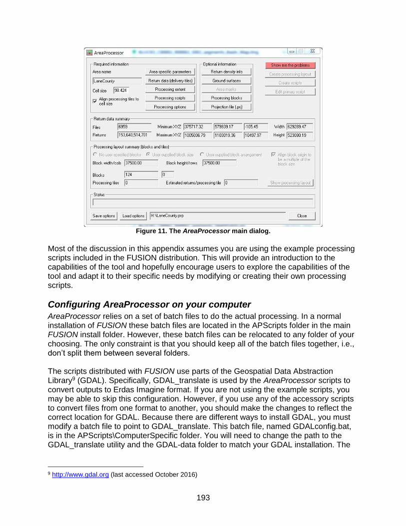
193

Figure 11. The AreaProcessor main dialog.

Most of the discussion in this appendix assumes you are using the example processing scripts included in the FUSION distribution. This will provide an introduction to the capabilities of the tool and hopefully encourage users to explore the capabilities of the tool and adapt it to their specific needs by modifying or creating their own processing scripts.

Configuring AreaProcessor on your computer

AreaProcessor relies on a set of batch files to do the actual processing. In a normal installation of FUSION these batch files are located in the APScripts folder in the main FUSION install folder. However, these batch files can be relocated to any folder of your choosing. The only constraint is that you should keep all of the batch files together, i.e., don’t split them between several folders. The scripts distributed with FUSION use parts of the Geospatial Data Abstraction Library9 (GDAL). Specifically, GDAL_translate is used by the AreaProcessor scripts to convert outputs to Erdas Imagine format. If you are not using the example scripts, you may be able to skip this configuration. However, if you use any of the accessory scripts to convert files from one format to another, you should make the changes to reflect the correct location for GDAL. Because there are different ways to install GDAL, you must modify a batch file to point to GDAL_translate. This batch file, named GDALconfig.bat, is in the APScripts\ComputerSpecific folder. You will need to change the path to the GDAL_translate utility and the GDAL-data folder to match your GDAL installation. The

9 http://www.gdal.org (last accessed October 2016)


194

following lines from the GDALconfig.bat file show the path for a typical stand-alone installation of GDAL.:

set GDAL_TRANSLATE_LOCATION=C:\Program Files\GDAL\gdal_translate set GDAL_DATA=C:\Program Files\GDAL\gdal-data

If you update your installation of FUSION you should turn off the option to install computer-specific configuration information in the installer to preserve your changes to the GDALconfig.bat file.

Preparing data for AreaProcessor

As with other FUSION tools, there is some preparation needed before you can process data using AreaProcessor. If ground surface models were provided as part of the acquisition, they will need to be converted into FUSION’s DTM format. If you are planning to create the ground surfaces as part of the processing this task is not needed. Depending on the options used in AreaProcessor to develop the processing tile layout, you may need to create a return density raster layer. This can be done using the Catalog utility with the /density option or with the ReturnDensity tool. In general, ReturnDensity is faster but if you are using Catalog to do a quality check of your data, the added time to create the return density layer is minimal. Refer to Appendix F: Using AreaProcessor to produce return density raster layers for example that builds return density layers using a workflow generated by AreaProcessor. If you use another, non-FUSION tool to create the return density layer, you may need to convert it into FUSION’s DTM format. The sample processing batch files include the calculation of several topographic metrics using ground surfaces. Some of these metrics (e.g. topographic position index) look beyond the edges of the acquisition to compute values for areas within the acquisition. You can provide a secondary, or “background”, ground surface model that coves the area outside the acquisition boundary. Such a surface will generally be lower resolution compared to the LIDAR-derived surfaces but will still provide surface data to make the metrics reasonably valid within the acquisition boundary. The logic in all of the FUSION tools will use elevations from the highest-resolution source provided and will only use the “background” surface values when there are no other elevation sources covering a point location. Point data delivered in either LAS or LAZ format is generally ready for processing. If you have data delivered in individual flight lines, you may want to retile the data to make processing more efficient. Data for entire flight lines typically has a very large extent but only a small area within the extent actually contains data. As the workflow clips data for processing, the large extent results in testing of every point in the flight line to see if it is within the new processing tile extent. By retiling the data, only points within the tiles that overlap the processing tile extent need to be considered. Refer to Appendix E: Retiling point data using AreaProcessor for a sample retiling procedure.

195

For large acquisitions with several thousand delivery tiles, you can increase processing efficiency for multi-core runs by separating the delivery tiles onto different physical drives. This helps prevent disk I/O from being the bottleneck in processing especially if drives are connected to different USB ports (instead of sharing the same port through a USB hub. If you have a solid state drive on your computer, you can also move the delivery data onto this drive to further increase processing efficiency. Finally, you can help balance the I/O load on your computer if you specify a different drive for outputs than the drive containing your data, If you are using vendor-supplied ground surfaces, you may want to subdivide the files into smaller pieces. Processing efficiency can be increased substantially by splitting large ground surfaces into smaller, more manageable tiles. FUSION provides the SplitDTM tool to do the splitting. Smaller tiles allow all of the FUSION tools to better manage loading of ground surface used when normalizing point elevations. IN general, ground tiles with 125,000 cells or less provide a good balance between the number of tiles and the overall processing efficiency.

Processing tile and block strategies

The basic strategy when deciding on tile and block sizes is that you want the number of returns in each tile to be such that all of the FUSION tools that you are using for processing will operate on the tile. In addition, you want block outputs to be small enough to work in other, non-FUSION analysis tools. Most FUSION tools will work with at least 60,000,000 returns. The IntensityImage program is the most restrictive but it should still work with 60,000,000 returns unless you are producing very high resolution (pixels less than 1m) images. If you need to produce such images, drop the target number of returns to 40,000,000. For blocks, you want the output raster data layers sized so they will work in other analysis tools. In general, I find that raster outputs smaller than 30,000 by 30,000 cells will work in most other tools. When considering the block sizes you also want to have enough blocks to take advantage of the computing capability of your computer. You want to have at least as many blocks as you have cores that you want to allocate to processing. In general, I find it convenient to use the same size blocks across different acquisitions (and to force the block origin to be a multiple of the block size). This way data products from adjacent acquisitions will align. The logic used to determine the processing order for blocks looks at the size of the individual blocks (actual area within the block extent that contains point data) and queues the largest blocks first. The starting order for “complete” blocks, i.e. those completely covered by return data, is randomized in an attempt to prevent having blocks that share the same delivery tiles from running concurrently. After the “complete” blocks, the remaining blocks are ordered by the amount of area within the block covered by point data. In general, processing will seem to go slower at the beginning of a run and then speed up as the “complete” blocks are finished. If you specify a block size that is a multiple of the desired tile size, the processing layout will be slightly more efficient because there will be fewer “slivers” near the edges of the blocks. In general, processing will be faster for layouts with fewer tiles so it is often

196

worthwhile to try different combinations of tile and block sizes (without changing the desired maximum number of returns per tile) to see if you can find a combination that produces the fewest tiles. The logic used to compute the tile layout includes an optimization component but it is based on the specified tile size so trying different tile sizes might lead to a better solution.

Processing batch files

The set of batch files provided as part of the FUSION installation provide an example of what you can do with AreaProcessor. The batch files generated by AreaProcessor call the batch files that the user specifies to do most of the actual work involved in processing. While these processing batch files are somewhat complicated, you can modify them to further customize processing options or add new products. Figure 12 shows the processing script dialog with the batch files for a typical processing run.

Figure 12. Processing script dialog showing the batch files used for a typical processing run

using AreaProcessor.

The basic structure of the processing flow is that you have batch files to accomplish the following tasks:

Provide basic configuration information (basic_setup.bat)

Perform any actions needed before block processing is started (preblock.bat)

Process a single block of return data (tile.bat)

Deal with results for each processing block (merge tile outputs, convert formats, move products to the final output folders) (posttile.bat)

Perform any actions needed after all blocks have been processed (final merging of outputs, convert format, move products to the final output folders) (postblock.bat)

197

If you just want to produce the “standard” set of FUSION metrics using 30 m cells, you really don’t need to change any of the batch files. If you want to add or remove some of the outputs, you can do this at the beginning of the basic_setup.bat file in the section labeled “Overall options to compute metrics”. In this section you turn options on (be setting them to TRUE) or off (by setting them to FALSE) to control the outputs produced during a run. These changes are easy to make. However, if you want to change the cell sizes, you will need to make several changes in the basic_setup.bat file. The cell size specified in AreaProcessor is used to align all of the processing tiles and blocks. It should always be the same as the cell size specified in the basic_setup.bat file. Normally, this is the cell size used for GridMetrics. The cell sizes for all other products (canopy surfaces, intensity images, ground surfaces and topographic metrics) should divide evenly into the cell size specified in AreaProcessor. Failure to do this will result in problems when the posttile.bat and postblock.bat files attempt to merge outputs. For data using imperial units, I have used the conversion of 1 meter = 3.2808 feet when computing cell sizes. I realize that this isn’t an exact conversion and it makes it hard to work between U.S. survey feet and international feet but this conversion provides a level of precision that is “computer friendly” when you are storing data in ASCII text format with limited decimal precision. You can do more precise conversions and include more decimal digits but doing so will likely result in alignment problems when adjacent blocks of data are merged.

Configuring the run for multiple processors

The most significant feature of AreaProcessor is its ability to generate workflows that run on several processors/cores. To accomplish this, AreaProcessor takes advantage of features in the Windows operating system that attempt to balance the load on the cores. AreaProcessor creates separate batch files for each processing block and then queues these batch files in a way that allows Windows to assign them to the least busy processor. The net effect is that block processing occurs in parallel thereby making processing much more efficient. Users can control the number of cores used for a job by specifying the number of processing streams in the processing options. Blocks are assigned to processing streams based on the area within the block that actually contains data in an attempt to balance the time needed to complete each processing stream. In addition, all processing streams contain logic that monitors the status of the entire processing job so they can launch post-processing tasks after all block processing is complete. Specifying too many cores can effectively swamp the computer making it unusable for any other tasks while the AreaProcessor scripts are running. In general, I have found that leaving 2-3 cores for the other tasks produces reasonably efficient processing while still allowing the computer to be used for other tasks. When determining the number of processing streams, you also should consider the amount of memory on your computer and specify a number of processing streams so each stream has at least 2 Gb of memory available for use.

198

What to do when something goes wrong

The logic used to check for errors is written into the batch files created by AreaProcessor. This logic is identical to the logic inserted by LTKProcessor so you can refer to Appendix C: Using LTKProcessor to Process Data for Large Acquisitions for details. When an error is detected, the processing tile is highlighted in red on the LTKStatusMonitorMDI display. You can view the processing log and determine the cause of the error. To do this simply click on the tile shown in red and then select the button labeled “Show tile status” in the lower right corner of the status display. This brings up the dialog shown in Figure 13. At the bottom of the dialog you can view the processing log for the tile. If you scroll to the end of the log, you might be able to determine the cause of the error. If the error is related to a DOS command or non-FUSION software, it may be harder to find the cause of the error.

Figure 13. Status information for a processing tile displayed in LTKStatusMonitorMDI.

The most common error during a processing run occurs when a processing tile doesn’t contain any point data. This happens most often around the edges of the data coverage when the return density layer used to compute the processing tile layout is of low resolution. Basically, the cells in the return density layer indicate that there are points within the tile extent but, in reality, there are no points in the cell that are within the extent. These error can be ignored and they will not affect the final outputs. The second most common error, and the most difficult to recover from, occurs when your computer is restarted during a processing run. When this happens, you can manually run the LTKStatusMonitorMDI program and load the primary batch file. This should show you the status of the processing job when the computer was restarted. It is possible to restart all of the processing steams but things get complicated when there were

199

processing tiles being clipped when the computer restarted. This leaves behind corrupt point files that will need to be deleted manually before restarting any processing. These files will be located in the same folder as the primary batch file. Given the difficulty and complexity of restarting a job that was interrupted by a system restart, it is often better to just restart the entire job by running the primary batch file again. The dialog shown in Figure 13 also provides command lines that can be used to correct a tile that had errors of restart a processing job. Each of these command lines should be run in the folder containing the master batch file for the processing run. If you find the source of an error associated with an individual tile and can correct the error, you can reprocess the tile using the command at the top of the dialog. You can copy this command from the dialog and paste it into a command prompt window to start the processing. You would use this first command if there are several tile that had errors running (run the reprocessing command for each tile). The second command in the dialog restarts processing with a specific tile and then runs all post-tile and post-block scripts. You would use this command to restart the processing if you only had one tile with an error. The third command runs to post-tile processing script for the processing block. The fourth command runs the post-processing for the processing stream. The fifth command runs the post-block processing script for the entire area. When errors occur but processing ran to completion, you need to reprocess each of the tiles that had errors using the first command. Then run the post-processing (third command) for each of the blocks that had tiles with error. Once all block post-processing is complete, you can use the fourth command to run post-processing for the processing stream. Finally, once all post-processing is done for the streams you can use the fifth command to run the final post-processing for the entire area. If you are monitoring the processing and notice that an error occurred in a single block, you can stop the associated processing stream and use the second command to restart the processing for the block. In this case, all of the post-processing tasks will be automatically run as blocks and processing streams finish.

200

Appendix E: Retiling point data using AreaProcessor

201

Using AreaProcessor to retile point files

There are situations where it is desirable to retile point data. For cases where points are delivered in very large files, processing can be slow because clipping operations need to read the entire file. Point file indexing can be used to speed up clipping operations but this results in a different point order data (at least this is true for FUSION but it may be possible to sort the outputs back into the original order in LAStools). For cases where points are delivered in separate files for each flight line, the rectangular extent for the tile can make it appear that there is data covering a much larger area so tiles are read unnecessarily when performing clipping operations. The options available in AreaProcessor allow you to create a tile layout where you have control over the tile size and the tile origin. You can use the multi-processor capability in some situations to improve the performance when retiling. You can also clip tiles with buffers (although a better approach is to clip tiles without buffers and then use these tiles with AreaProcessor and specify a buffer around the temporary tiles it creates for processing). The only real “trick” when building a run stream to retile data is that the tile processing batch file has nothing to do because the commands to clip new data tiles are written into the batch files created by AreaProcessor. This does mean that you need to use a special tile processing batch file that doesn’t do any processing. In addition, the cell size doesn’t really matter so long as the tile size is a multiple of the cell size. If you have data in large files or flight lines, the best strategy is to clip a new set of tiles that are still fairly large and then use these tiles to clip a final set of smaller tiles. The reason for the two-step process is that the time to clip a tile from large files is almost independent of the new tile size. This means that clipping a small tile from a few very large files will take just as long as clipping a large tile. If you do the initial clip to create set of new (still large) tiles and then use these tiles to clip small tiles, the small tile clipping will go faster. In most circumstances, the total time to produce the small tiles will be shorter compared to clipping the small tiles in a single pass. For clipping tiles when you have a few very large files you generally want to use a single run stream to avoid having multiple processes trying to simultaneously read from the same file. For the processing scripts you need to specify the output folder, primary batch file name, folder with secondary batch files, and the tile processing batch file (the one that doesn’t do anything). None of the other batch files are needed. Figure 14 shows an example of the processing scripts needed when retiling data when you have return density layer(s) available. If you don’t have return density layers, you would use option 2 to compute the processing tile layout.

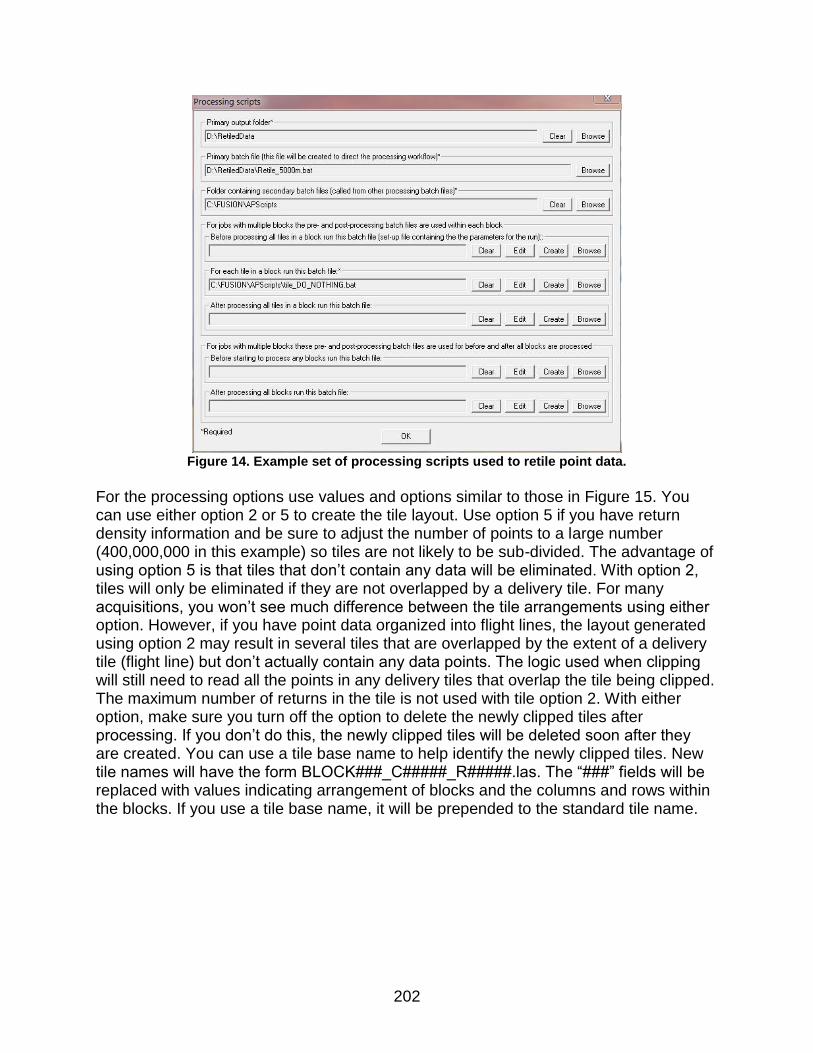
202

Figure 14. Example set of processing scripts used to retile point data.

For the processing options use values and options similar to those in Figure 15. You can use either option 2 or 5 to create the tile layout. Use option 5 if you have return density information and be sure to adjust the number of points to a large number (400,000,000 in this example) so tiles are not likely to be sub-divided. The advantage of using option 5 is that tiles that don’t contain any data will be eliminated. With option 2, tiles will only be eliminated if they are not overlapped by a delivery tile. For many acquisitions, you won’t see much difference between the tile arrangements using either option. However, if you have point data organized into flight lines, the layout generated using option 2 may result in several tiles that are overlapped by the extent of a delivery tile (flight line) but don’t actually contain any data points. The logic used when clipping will still need to read all the points in any delivery tiles that overlap the tile being clipped. The maximum number of returns in the tile is not used with tile option 2. With either option, make sure you turn off the option to delete the newly clipped tiles after processing. If you don’t do this, the newly clipped tiles will be deleted soon after they are created. You can use a tile base name to help identify the newly clipped tiles. New tile names will have the form BLOCK###_C#####_R#####.las. The “###” fields will be replaced with values indicating arrangement of blocks and the columns and rows within the blocks. If you use a tile base name, it will be prepended to the standard tile name.

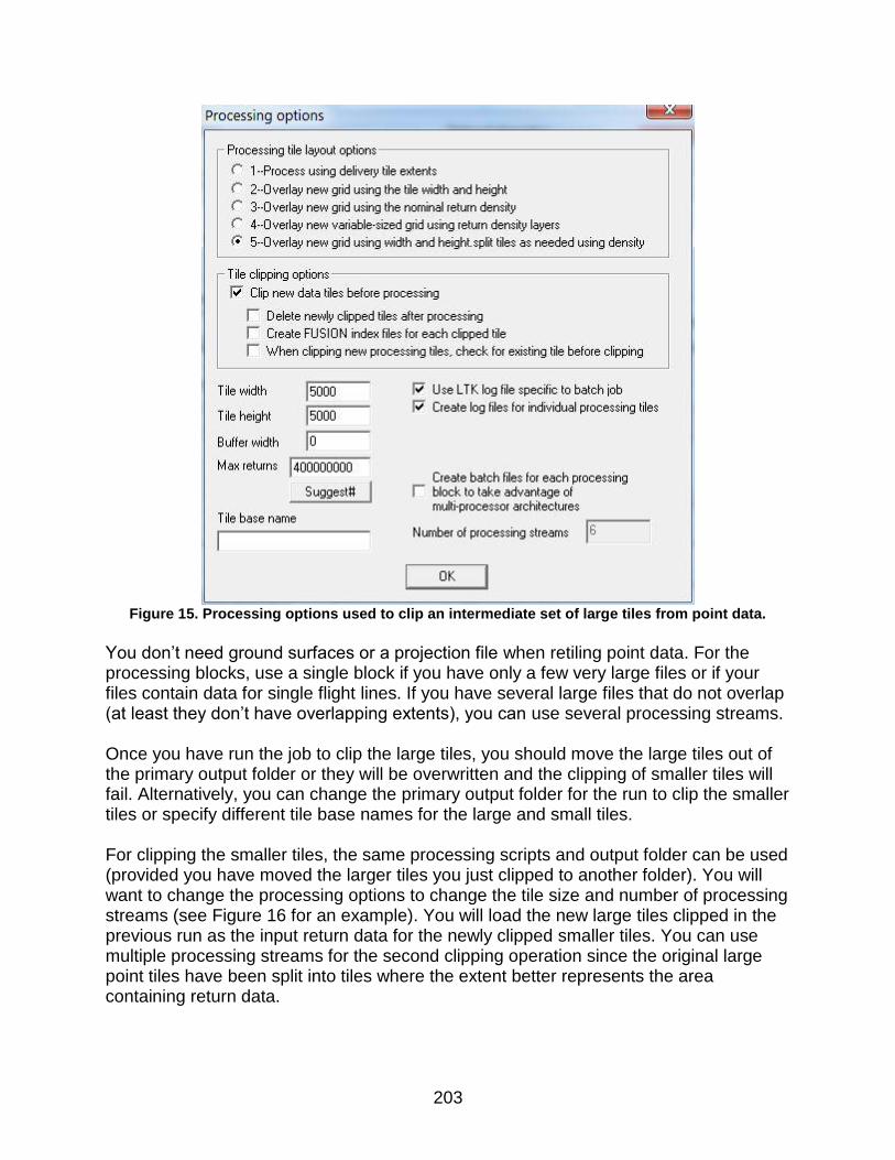
203

Figure 15. Processing options used to clip an intermediate set of large tiles from point data.

You don’t need ground surfaces or a projection file when retiling point data. For the processing blocks, use a single block if you have only a few very large files or if your files contain data for single flight lines. If you have several large files that do not overlap (at least they don’t have overlapping extents), you can use several processing streams. Once you have run the job to clip the large tiles, you should move the large tiles out of the primary output folder or they will be overwritten and the clipping of smaller tiles will fail. Alternatively, you can change the primary output folder for the run to clip the smaller tiles or specify different tile base names for the large and small tiles. For clipping the smaller tiles, the same processing scripts and output folder can be used (provided you have moved the larger tiles you just clipped to another folder). You will want to change the processing options to change the tile size and number of processing streams (see Figure 16 for an example). You will load the new large tiles clipped in the previous run as the input return data for the newly clipped smaller tiles. You can use multiple processing streams for the second clipping operation since the original large point tiles have been split into tiles where the extent better represents the area containing return data.

204

Figure 16. Processing options use to clip the final tiles from point data.

When creating the processing blocks for the final tiling operation, subdivide the area using a block width and height that are multiples of the tile size. Once you have computed the tile arrangement, check the processing layout to verify that you are getting tiles that make sense. If you are using return density layers, you shouldn’t have tiles outside the area covered by point data. If you are not using return density layers, you may have new tiles that end up with no data. For these tiles, the status monitor will show a red tile indicating that an error occurred. You can ignore these errors as they simply indicate that there were no points clipped in the new tile. Once you have run the job to clip the smaller tiles, you can move the smaller tiles to their final location. The tile naming will again reflect the arrangement of processing blocks. Unfortunately, there is no good strategy for renaming the tiles to reflect an overall row/column reference grid for the entire data set.

205

Appendix F: Using AreaProcessor to produce return density raster layers

206

To develop the most efficient layout of processing tiles, AreaProcessor uses a raster data layer describing the total number of returns in each cell. This layer can be generated using the Catalog tool but, for large data sets, you must use a very large cell size. This coarse resolution limits the algorithm used to computer the tile layout. The following describes the steps and configuration needed to use AreaProcessor to create a workflow that builds return density layers. The workflow produces a set of high-resolution tiles that can then be used to develop a processing workflow. The basic strategy is to build a processing layout so that the return density layers are created for each processing block without clipping new point tiles. To do this, the processing tiles and blocks will be the same size and you will use a tiling option that simply overlays a grid on the data extent. The basic steps to create the workflow are:

Set the cell size on AreaProcessor’s main dialog (set to 50 m for this example)

Load all the point data files into the Return data

Set the processing options as shown in Figure 17 (tile size may vary depending

on units and cell size). For this example, the final tiles will only be 500 by 500

cells. For a “real” configuration, try to specify a combination of the cell size and

tile size to produce outputs smaller than 2500 by 2500 cells. Be sure to uncheck

the option to clip data tiles before processing.

Figure 17. Processing options used to create return density raster layers.

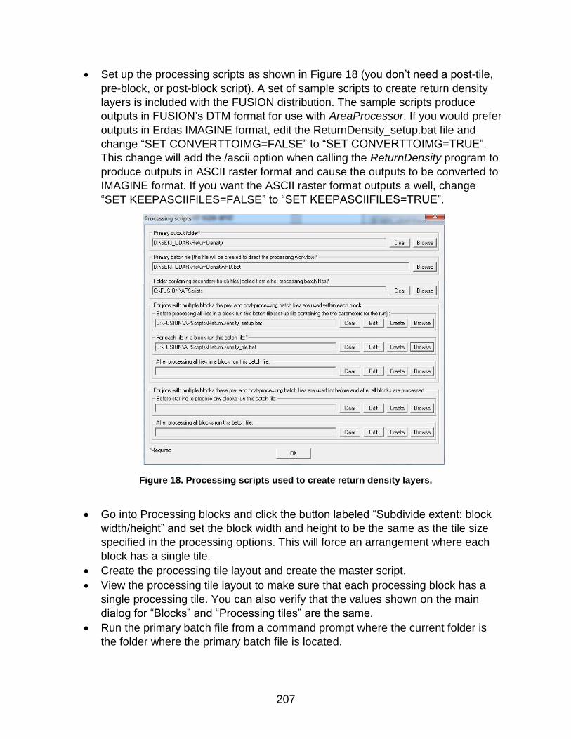
207

Set up the processing scripts as shown in Figure 18 (you don’t need a post-tile,

pre-block, or post-block script). A set of sample scripts to create return density

layers is included with the FUSION distribution. The sample scripts produce

outputs in FUSION’s DTM format for use with AreaProcessor. If you would prefer

outputs in Erdas IMAGINE format, edit the ReturnDensity_setup.bat file and

change “SET CONVERTTOIMG=FALSE” to “SET CONVERTTOIMG=TRUE”.

This change will add the /ascii option when calling the ReturnDensity program to

produce outputs in ASCII raster format and cause the outputs to be converted to

IMAGINE format. If you want the ASCII raster format outputs a well, change

“SET KEEPASCIIFILES=FALSE” to “SET KEEPASCIIFILES=TRUE”.

Figure 18. Processing scripts used to create return density layers.

Go into Processing blocks and click the button labeled “Subdivide extent: block

width/height” and set the block width and height to be the same as the tile size

specified in the processing options. This will force an arrangement where each

block has a single tile.

Create the processing tile layout and create the master script.

View the processing tile layout to make sure that each processing block has a

single processing tile. You can also verify that the values shown on the main

dialog for “Blocks” and “Processing tiles” are the same.

Run the primary batch file from a command prompt where the current folder is

the folder where the primary batch file is located.

208

Appendix G: Converting ESRI GRID data to ASCII raster format using GDAL

209

Overview

Surface data, including bare-ground and canopy surface models, are often provided in ESRI’s GRID format. While this format is common to users of ESRI’s products, it is a proprietary format that is not used by many applications. The Geospatial Data Abstraction Library (GDAL) is an open-source library and collection of applications (http://www.gdal.org/) that can read surface data stored GRID format and convert it to other formats. The most useful conversion for FUSION users is that from GRID to ASCII raster format used by the ASCII2DTM program. In general, conversion from GRID to ASCII raster format using GDAL is faster than the same conversion using the RasterToASCII command in ArcMap. In addition, conversion of several GRID files can files can be accomplished using a batch file containing a simple FOR loop that process all folders (GRID layers) in an acquisition.

Converting Data from GRID to ASCII Raster Format

GDAL provides the gdal_translate utility to convert raster data between different formats. This utility is useful and allows this conversion without any need for ESRI’s GIS products. Complete documentation for gdal_translate can be found here: http://www.gdal.org/gdal_translate.html. While gdal_translate provides a number of useful features, the most important options when converting GRID data for use by ASCII2DTM are:

-co FORCE_CELLSIZE=YES

-co DECIMAL_PRECISION=4 (# of decimal digits in ASCII raster output)

The first option forces grid cells to be square and the second specifies the number of decimal digits “printed” to the ASCII raster files. The DECIMAL_PRECISION option can dramatically affect the size of the output files so you should not specify excessive precision. Three or four decimal digits are usually sufficient for airborne LIDAR data. When converting GRID data, the input “file” is simply the folder name used to store all of the files associated with the GRID layer. Gdal_translate will find the file in this folder that contains the actual grid values and convert these to the ASCII raster format. Syntax for the command line to convert data stored in GRID format into ASCII raster format is:

gdal_translate –co FORCE_CELLSIZE=YES –co DECIMAL_PRECISION=4 –of AAIGrid

folder_name output_file.asc

The –co options are described above. The –of AAIGrid option specifies that the output is to be ASCII raster format. folder_name specifies the name of the folder containing the GRID layer and output_file.asc specifies the desired name for the output data. The “.asc” extension is not mandatory but this is the extension expected by the ASCII2DTM utility.


http://www.gdal.org/gdal_translate.html

Documents

Analysis and Forest Service Visualizationforsys.sefs.uw.edu/Software/FUSION/FUSION_manual.pdf326- W, Whitten Building, 14th and Independence Avenue, SW, Washington, DC 20250-9410 or