ANALYSIS AND EXTENSION OF THE FURTER EQUATION, AND …relative volatility. This approach allowed systematic extensions of the Furter equation and a brief review of the theoretical

Brazilian Journalof ChemicalEngineering

ISSN 0104-6632Printed in Brazil

www.abeq.org.br/bjche

Vol. 34, No. 02, pp. 607 - 621, April - June, 2017dx.doi.org/10.1590/0104-6632.20170342s20150102

*To whom correspondence should be addressed

ANALYSIS AND EXTENSION OF THE FURTER EQUATION, AND ITS APPLICATION IN THE

SIMULATION OF SALINE EXTRACTIVE DISTILLATION COLUMNS

E. O. Timmermann1† and C. R. Muzzio2*

1Instituto de Investigación y Desarrollo, Academia Nacional de Ciencias de Buenos Aires,Av. Alvear 1711, Buenos Aires, Argentina.

† passed away.2Departamento de Química, Facultad de Ingeniería, Universidad de Buenos Aires,

Paseo Colón 850, Buenos Aires, Argentina.Phone: +54 11 4343-0893E-mail: [email protected]

(Submitted: February 25, 2015; Revised: November 7, 2015; Accepted: February 5, 2016)

Abstract – Simulation of saline extractive distillation columns is a difficult task owing to the high nonlinearity of the rigorous models that represent these systems. The use of simple models to obtain initial estimates of equilibrium compositions may improve the stability and rate of convergence. One of the simplest models to study the vapor-liquid equilibrium of binary liquid mixtures + salt systems is the Furter equation. This model was analyzed in the present work by means of the incorporation of activity coefficient models in the ratio of relative volatility. This approach allowed systematic extensions of the Furter equation and a brief review of the theoretical basis of the original equation. As a result of these extensions, two simple equations were proposed and tested with experimental data from 20 systems, including binary liquid mixtures + salt systems and binary liquid mixtures + ionic liquid systems. Finally, one of these proposed equations was incorporated into the GKTM software in order to assess the utility of these simple models in the simulation of saline extractive distillation columns. The obtained results showed a significant improvement over the previous algorithm.Keywords: Electrolyte; Salt effect; Furter equation; Regular solution; Solvation; Extractive Distillation; Simulation

INTRODUCTION

Distillation is one of the most important unit operations in chemical engineering, owing to its frequent use in separation processes and the cost associated with them in the chemical industry (Gmehling, 2009). Sometimes, the separation of liquid mixtures through distillation is hindered by the existence of an azeotropic point. As is well known, conventional distillations are not able to purify binary liquid mixtures beyond the concentration of this

azeotropic point. Nonetheless, distillation of mixtures that present an azeotropic point can be improved by using a separating agent, sometimes called an entrainer (Kiss & Suszwalak, 2012; Matsuda et al., 2011; Bastos et al., 2015; Zhang et al., 2015). The entrainer is added in order to change the volatility of the components, and depending on its effects on the mixture, it leads mainly to two different distillations: azeotropic or extractive distillation. In the first case, the entrainer induces minimum-boiling azeotropes and liquid-liquid immiscibilities to modify

Brazilian Journal of Chemical Engineering

E. O. Timmermann and C. R. Muzzio608

the behavior of the mixture and allow the distillation. In the second case, the entrainer is a relatively non-volatile component that allows the distillation by shifting or even eliminating the binary azeotrope, as a result of its differential affinity with the components of the original binary liquid mixture. In comparison with azeotropic distillation, extractive distillation is simpler, can use more entrainers, and is less expensive than azeotropic distillation (Tassios, 1972). The use of high-boiling point solvents or non-volatile components in extractive distillations leads to lower energy consumptions in comparison to azeotropic distillation, because the entrainer does not need to be vaporized (Kiss & Suszwalak, 2012). In addition, the third component added in extractive distillations is often safer than the organic solvents commonly used in azeotropic distillation; this is the case, for example, of saline extractive distillations, where the entrainer is a salt, which presents very low toxicity and flammability. Although not as safe as inorganic salts as a consequence of a higher toxicity, the use of ionic liquids has recently become an interesting alternative as entrainer in SED because of their recognized advantages: in addition to their low vapor pressure, which allows an efficient recovery, ionic liquids are less corrosive and have higher solubility than inorganic salts (Bastos et al., 2015; Calvar et al., 2007; Pereiro et al., 2012; Vicent Orchillés et al., 2008; Vicent Orchillés et al., 2011, Zhang et al., 2015).

The addition of small quantities of dissolved salts or ionic liquids (Pereiro et al., 2012) can shift or even eliminate the presence of the azeotropic point, thus making it possible to obtain high purity products from the top of the distillation column. The effect of the separating agent on the mixed solvent equilibrium is known as the salt effect. This salt effect of dissolved salts on liquid mixtures had already been studied and reported at the end of the nineteenth century (Kablukov, 1891; Miller, 1897) , then followed by systematic investigations on the subject from the 1950’s (Cardoso and O’Connell, 1987; Jaques and Furter, 1974; Loehe and Donohue, 1997; Robinson and Stokes, 1959). The appearance of new materials that better withstand the highly corrosive medium associated with salt systems, the fact that the addition of salts to azeotropic mixtures avoids the requirement of a third solvent, which is usually harmful to the environment, and the increasing necessity of processes with low energy consumption, leads to a renewed interest in saline extractive distillation (SED). In this direction, several papers (Llano-Restrepo and Aguilar-Arias, 2003; Muzzio and Timmermann, 2014; Pinto et al., 2000) have been recently published in order to better understand and optimize the SED process through the use of computer simulators. Computer simulation arose as one of the principal tools to improve the knowledge of the SED process, but this tool requires reliable models that allow the calculation of the phase equilibrium behavior of the system to be separated.

Several models were published as part of the aforementioned investigations, e.g., E-NRTL (Chen and Song, 2004; Mock et al., 1986), LiQUAC-E (Li et al., 1994; Mohs and Gmehling, 2013) and the Extended UNIQUAC (Iliuta et al., 2000; Sander et al., 1986). These models are capable of very accurate VLE data regression by considering the Gibbs energy as the combination of three different range contributions: long-range, middle-range and short-range. Since some contributions are mainly theoretical (for example Debye-Hückel) and other ones are semi-empirical, with several parameters that have to be regressed from VLE data, these are limited to the range, quantity and precision of the correlated data; any extrapolation may lead to significant deviations and should be avoided. In addition, the regression of parameters is not always clear (Muzzio and Timmermann, 2014) and, often, the parameter values required for a proper data regression lack physical meaning.

On the other hand, a very useful and simple relationship was proposed by Johnson and Furter (1960):

This equation relates the ratio of relative volatilities with (αs) and without (α0) salt present to the salt concentration in the liquid phase (x3). Owing to its simplicity and capacity to correlate experimental data, this model has been studied and extended by different authors (Hashitani and Hirata, 1969; Wu et al., 1999; Wu et al., 2001). In spite of not having a deep thermodynamic basis, the fact that only one constant is needed for a binary liquid mixture + solute system gives this equation an advantage over other semi-empirical methods like E-NRTL, which requires the regression of nine parameters for a binary liquid mixture + salt system. Nevertheless, as stated by Meranda and Furter (1971), the value of k is not expected to remain constant when the solvent compositions are varied owing to the interactions between the different components in the liquid phase (including volatile and nonvolatile). Understanding this limitation in the Furter equation, Hashitani and Hirata (1969) reported an empirical model which takes into account these interactions within the salt system, related not only to the electrolyte composition but also to the proportion of components in the binary liquid mixture:

where z+ is the mole fraction of the more volatile component in the liquid phase (salt free basis).

The current interest in extending the Furter equation throughout the entire composition range of the two volatile

ln 𝛼𝑠 𝛼0⁄ = 𝑘 . 𝑥3

ln 𝛼𝑠 𝛼0⁄ = 𝑘1𝑘2𝑧+.

𝑥31− 𝑥3

(1)

(2)

Brazilian Journal of Chemical Engineering Vol 34, No 02, pp. 607 - 621, April - June, 2017

Analysis and Extension of The Furter Equation, and Its Application in The Simulation of Saline Extractive Distillation Columns

609

components leads to more recent developments (Wu et al., 1999; Wu et al., 2001). For example, the interesting model proposed by Wu et al. (1999) includes a quadratic term and a second constant, i.e.:

The additional term improves the correlation of the model, as expected. Surprisingly, the proposed model does not include a term related to the proportion of the components in the binary liquid mixture.

In the present work, the Furter equation was analyzed from the consideration of activity models in the ratio of solvent volatilities. The analysis not only increased the knowledge on the Furter equation, but also set a basis for systematic extensions of this model. As a result of this approach, two new extensions of the Furter equation were proposed. One of these extensions was incorporated into a SED column simulator (GKTM, Muzzio and Timmermann, 2014) in order to improve the stability and rate of convergence of the previous algorithm, by obtaining better initial estimates of the vapor compositions at each stage. The simulation results proved that the inclusion of Furter extended models into the simulator software led to a more efficient algorithm.

FURTER EQUATION ANALYSIS

The expressions of fugacity and relative volatility of the volatile components in a binary liquid mixture + salt systems can be combined as following:

The ratio of relative volatilities (binary mixture and binary mixture-salt systems) is defined as:

where zi is the mole fraction of component i on a salt-free basis.

At moderate pressures, Eq. (5) can be simplified with negligible error considering an ideal gas in the vapour phase and replacing the fugacity of pure liquid by the vapour

pressure of the pure liquid at the considered temperature:

Replacing in (6):

If the temperature variation in the system after adding the salt is low enough, or if the relationships between pressures for both volatile components after adding the salt are similar, the effect related with vapour pressures of the pure liquids can be neglected in comparison to the effect related with activity coefficients. As a result, the Furter equation may be expressed as:

It is convenient to introduce some additional useful definitions:

ln 𝛼𝑠 𝛼0⁄ = 𝑘1 .𝑥3 + 𝑘2 . 𝑥32

𝑃𝜙�𝑖𝑦𝑖 = 𝑓𝑖𝑜𝛾𝑖𝑥𝑖

𝑦𝑖 =𝑓𝑖𝑜𝛾𝑖𝑥𝑖𝑃𝜙�𝑖

𝛼𝑠𝛼0

=𝑦1,𝑠𝑧1,𝑠

𝑧2,𝑠𝑦2,𝑠

𝑦1,0𝑥1,0

𝑥2,0𝑦2,0

� =𝑦1,𝑠𝑦1,0

𝑦2,0𝑦2,𝑠

𝑦𝑖 =𝑃𝑖𝑜𝛾𝑖𝑥𝑖𝑃

𝛼𝑠𝛼0

=𝛾1 ,𝑠𝛾2 ,0𝑥1,𝑠𝑥2,0𝛾1 ,0𝛾2 ,𝑠𝑥2,𝑠𝑥1,0

𝑃1𝑜 𝑇𝑠 𝑃2𝑜 𝑇𝑃2𝑜 𝑇𝑠 𝑃1𝑜 𝑇

=𝛾1 ,𝑠𝛾2 ,0𝛾1 ,0𝛾2 ,𝑠


ln𝛼𝑠𝛼0

= ln𝛾1,𝑠𝛾2 ,0𝛾1,0𝛾2 ,𝑠

𝛼𝑠𝛼0

=𝛾1 ,𝑠𝛾2 ,0𝑥1,𝑠𝑥2,0𝛾1 ,0𝛾2 ,𝑠𝑥2,𝑠𝑥1,0


=𝛾1 ,𝑠𝛾2 ,0𝛾1 ,0𝛾2 ,𝑠


𝑧1 ≡𝑛1𝐿

𝑛1𝐿 + 𝑛2𝐿= 1− 𝑧2 =

𝑥11 −𝑥3

𝑧3 ≡𝑛3𝐿

𝑛1𝐿 + 𝑛2𝐿=

𝑥31− 𝑥3

𝑦1 =𝑛1𝑉

𝑛1𝑉 + 𝑛2𝑉= 1 −𝑦2

𝛽 =1

1 + 𝑧3

𝑥𝑖 = 𝛽. 𝑧𝑖

(3)

(4)

(5)

(6)

(7)

(8)

(9)

(10)

(11)

(12)

(13)

(14)



where z1 and z3 are the mole fractions of component 1 and salt respectively, on a salt free basis. The usual mole fractions of component 1 and salt are designed x1 and x3, respectively.

Regular solution model

The simplest expression for the activity coefficient is the regular solution model. For the components in binary liquid mixtures, the expressions are the following (Prigogine and Defay, 1954):

For ternary mixtures (two volatile components and a salt), if the electrolyte is regarded as a solute, the regular solution model can be expressed as:

where A ≡ A12 = A21; ∆A ≡ A13 – A23, the subscripts 1 and 2 are reserved for the volatile components, and the subscript 3 for the salt.

Then, Eq. (15a) and (15b) can be related by:

Similarly, Eq. (17a) and (17b) can be related by:

Finally, by considering equations (6-19), and expressing the logarithm of the ratio of relative volatilities with and without salt present, the following expressions can be derived:

From Eq. (13), β may be approximated by 1 when z3 is low enough and, as a consequence, Eq. (21) can be reduced to the usual Furter expression, where k = ∆A. Nonetheless, if this approximation is not considered, and taking into account that (β – 1) = –z3β, the salt parameter can be expressed from Eq. (21) as

Equation (22) shows the functionality of the parameter with the composition of the volatile components. A more useful expression of Eq. (21) and Eq. (22) is the Furter-Regular Solution (FRS) equation

ln 𝛾1 ,0 = 𝑥2,02 .𝐴12 = 𝑧22 .𝐴12

ln 𝛾2 ,0 = 𝑥1,02 .𝐴21 = 𝑧12 .𝐴21

ln 𝛾1 ,𝑠 = 𝑥2,𝑠2 .𝐴12 + 𝑥3,𝑠

2 .𝐴13 + 𝑥2,𝑠 .𝑥3,𝑠 . 𝐴12 + 𝐴13 − 𝐴23

ln 𝛾2 ,𝑠 = 𝑥1,𝑠2 .𝐴21 + 𝑥3,𝑠

2 .𝐴23 + 𝑥1,𝑠 .𝑥3,𝑠 . 𝐴21 + 𝐴23 − 𝐴13

ln 𝛾1 ,𝑠 = 𝛽2 𝑧22.𝐴 + 𝑧32 .𝐴13 + 𝑧2 .𝑧3 . 𝐴+ Δ𝐴

ln 𝛾2 ,𝑠 = 𝛽2 𝑧12 .𝐴 + 𝑧32 .𝐴23 + 𝑧1.𝑧3 . 𝐴− Δ𝐴

ln𝛾1,0𝛾2 ,0

= 1 − 2. 𝑧1 .𝐴

ln 𝛾1 ,𝑠 = 𝑥2,𝑠2 .𝐴12 + 𝑥3,𝑠

2 .𝐴13 + 𝑥2,𝑠 .𝑥3,𝑠 . 𝐴12 + 𝐴13 − 𝐴23

ln 𝛾2 ,𝑠 = 𝑥1,𝑠2 .𝐴21 + 𝑥3,𝑠

2 .𝐴23 + 𝑥1,𝑠 .𝑥3,𝑠 . 𝐴21 + 𝐴23 − 𝐴13

ln 𝛾1 ,𝑠 = 𝛽2 𝑧22.𝐴 + 𝑧32 .𝐴13 + 𝑧2 .𝑧3 . 𝐴+ Δ𝐴

ln 𝛾2 ,𝑠 = 𝛽2 𝑧12 .𝐴 + 𝑧32 .𝐴23 + 𝑧1.𝑧3 . 𝐴− Δ𝐴

ln𝛾1 ,𝑠𝛾2 ,𝑠

= 𝛽2 𝑧22 .𝐴+ 𝑧32 .𝐴13 + 𝑧2 .𝑧3 . 𝐴+ Δ𝐴 − 𝑧12.𝐴 + 𝑧32 .𝐴23 + 𝑧1 .𝑧3 . 𝐴− Δ𝐴 =

= 𝛽2 1− 2. 𝑧1 .𝐴 + 1− 2. 𝑧1 .𝑧3𝐴+ 𝑧32 .Δ𝐴+ 𝑧3Δ𝐴 = 𝛽 𝐴. 1− 2.𝑧1 + 𝑧3Δ𝐴 ln𝛾1 ,𝑠𝛾2 ,𝑠




= 𝛽2 1− 2. 𝑧1 .𝐴 + 1− 2. 𝑧1 .𝑧3𝐴+ 𝑧32 .Δ𝐴+ 𝑧3Δ𝐴 = 𝛽 𝐴. 1− 2.𝑧1 + 𝑧3Δ𝐴

ln𝛾1 ,𝑠𝛾2 ,𝑠




= 𝛽2 1− 2. 𝑧1 .𝐴 + 1− 2. 𝑧1 .𝑧3𝐴+ 𝑧32 .Δ𝐴+ 𝑧3Δ𝐴 = 𝛽 𝐴. 1− 2.𝑧1 + 𝑧3Δ𝐴

ln𝛼𝑠𝛼0

= ln𝛾1,𝑠𝛾2 ,0𝛾1,0𝛾2 ,𝑠

=𝛽 𝐴. 1− 2. 𝑧1 + 𝑧3Δ𝐴 − 1− 2. 𝑧1 .𝐴

ln𝛼𝑠𝛼0

= 𝛽 − 1 𝐴. 1− 2.𝑧1 + 𝑥3Δ𝐴

ln𝛼𝑠𝛼0

= ln𝛾1,𝑠𝛾2 ,0𝛾1,0𝛾2 ,𝑠

=𝛽 𝐴. 1− 2. 𝑧1 + 𝑧3Δ𝐴 − 1− 2. 𝑧1 .𝐴

ln𝛼𝑠𝛼0

= − 1− 2.𝑧1 𝐴+ Δ𝐴 .𝑥3=𝑘.𝑥3

ln𝛼𝑠𝛼0

= Δ𝐴− 𝐴 . 𝑥3+2𝐴β

𝑥1.𝑥3 = 𝑘.𝑥3+𝑘′.𝑥1𝑥3

ln𝛼𝑠𝛼0

= Δ𝐴− 𝐴 . 𝑥3+2𝐴β

𝑥1.𝑥3 = 𝑘.𝑥3+𝑘′.𝑥1𝑥3

(15a)

(15b)

(18)

(19)

(20)

(22)

(23)

(16a)

(16b)

(17a)

(17b)

(21)



611

where β has been considered constant, since it is mostly between 0.9 and 1.

In comparison with the model proposed in Wu’s work (Wu et al., 1999), Eq. (23) includes a term of interaction between solvent and solute that could explain its better capacity of regression.

Solvation model

More accurate models can be introduced in Eq. (9). If the excess Gibbs energy is calculated as the sum of long-range (LR) and short-range (SR) contributions,

the expression for calculation of the activity coefficient of solvent i is:

In this approach, the long-range contribution is related to the interactions between ions, while the short-range (SR) contribution is related to interactions between all the species. Therefore, in a mixture without ions, only the short-range contribution should be considered. Replacing Eq. (25) in Eq. (9), the following equation is obtained:

In this equation, yi,0 was replaced with yi,0SR because

there are no ions in the system.The Debye-Hückel (DH) model is considered to take

into account the long-range (LR) contribution in mixed solvent systems. If the partial molar volume of the solvent in the solution is approximated as the molar volume of the pure solvent, the LR logarithm can be expressed as (Li et al., 1994)

where Mi is the molecular weight of the solvent, di is the molar density of the pure solvent i, d is the mixed-solvent molar density; I, A and b are DH parameters, where I = 0.5 Σimizi

2, mi is the molality of ion i, vi is the salt stoichiometric

number, A = 1.3278.105 d0.5/(DT)1.5 and b = 6.360.d0.5/(DT)0.5.

Nevertheless, if the DH expression is considered to have negligible effect on the phase equilibrium behaviour, as stated by Chen and Evans (1986), especially in systems with high salt concentration (m>0.1), Eq. (26) can be simplified to:

As a result, the objective is to find the effect of the salt on the activity coefficient of each solvent for the SR contribution. An interesting approach to consider in Eq. (28) is related to the solvation of ions, in which the effect of the salt is taken into account from the decrease of free solvent molecules by the solvated molecules (Robinson and Stokes, 1959). In this approach, the number of moles (ni,F) of free solvent i is given by:

and the mole fraction (xi,F) of free solvent i can be expressed as:

wherein hi is the solvation number of the salt with pure component of the mixed solvent system i and n3 is the number of moles of salt. For binary liquid mixtures + salt systems, Eq. (30) yields:

For the resolution of this solvation model, the following general thermodynamic rule is applied (Nothnagel et al., 1973; Prigogine and Defay, 1954). At equilibrium, when a fluid exists in several associated forms, the chemical potential (µi,F) of the monomer (free) molecule is equal to the stoichiometric (or apparent) chemical potential (µi,),

𝐺𝐸 = 𝐺𝐸,𝐿𝑅 + 𝐺𝐸,𝑆𝑅

ln 𝛾𝑖 = ln 𝛾𝑖𝐿𝑅 + ln 𝛾𝑖𝑆𝑅 = ln 𝛾𝑖𝐿𝑅𝛾𝑖𝑆𝑅

ln𝛼𝑠𝛼0

= ln𝛾1 ,𝑠𝛾2 ,0𝛾1 ,0𝛾2 ,𝑠

=ln𝛾1 ,𝑠𝐿𝑅𝛾1 ,𝑠

𝑆𝑅𝛾2 ,0𝑆𝑅

𝛾2 ,𝑠𝐿𝑅𝛾2,𝑠

𝑆𝑅𝛾1,0𝑆𝑅

ln 𝛾𝑖𝐿𝑅 = 2𝐴𝑀𝑖𝑑 𝑏3𝑑𝑖⁄ 1 + 𝑏𝐼1 2⁄ − 1 + 𝑏𝐼1 2⁄ −1− 2ln 1 + 𝑏𝐼1 2⁄

ln 𝛾𝑖𝐿𝑅 = 2𝐴𝑀𝑖𝑑 𝑏3𝑑𝑖⁄ 1 + 𝑏𝐼1 2⁄ − 1 + 𝑏𝐼1 2⁄ −1− 2ln 1 + 𝑏𝐼1 2⁄

ln𝛼𝑠𝛼0

= ln𝛾1 ,𝑠𝛾2 ,0𝛾1 ,0𝛾2,𝑠

=ln𝛾1 ,𝑠𝑆𝑅𝛾2 ,0

𝑆𝑅

𝛾2 ,𝑠𝑆𝑅𝛾1,0

𝑆𝑅

𝑛𝑖 ,𝐹=𝑛𝑖−ℎ𝑖𝑛3

𝑥𝑖,𝐹=𝑛𝑖−∑ ℎ𝑖𝑖 𝑛3

∑ 𝑛𝑗𝑗 + 𝜈3 −∑ ℎ𝑗𝑗 𝑛3=

𝑧𝑖−∑ ℎ𝑖𝑖 𝑧31 + 𝜈3 − ∑ ℎ𝑗𝑗 𝑧3

; j =1,2

𝑥𝑖,𝐹=𝑛𝑖−∑ ℎ𝑖𝑖 𝑛3

∑ 𝑛𝑗𝑗 + 𝜈3 −∑ ℎ𝑗𝑗 𝑛3=

𝑧𝑖−∑ ℎ𝑖𝑖 𝑧31 + 𝜈3 − ∑ ℎ𝑗𝑗 𝑧3

; j =1,2

𝑥𝑖,𝐹=𝑧1− ℎ1 + ℎ2 𝑧3

1 + 𝜈3 − ℎ1 − ℎ2 𝑧3

𝜇𝑖=𝜇𝑖 ,𝐹

(24)

(25)

(26)

(27)

(28)

(29)

(30)

(31)



In the case under study, the chemical potential of the free solvent molecule is equal to the chemical potential of solvent on a stoichiometric basis, an expression which yields:

If the free solvent non-ideality is considered to be only due to electrostatic forces (DH) with ions and the interaction with the other solvent, then the activity coefficient can be rearranged from Eq. (33) as

For a binary system, Eq. (34) can be written as:

In the present work, hi is calculated as a function of zi, i.e., hi = hi

∞zi2 where hi

∞ is the solvation number of salt with component i at infinite dilution of the salt. Replacing Eq. (34) in Eq. (28), the Furter-Solvation (FS) model is obtained:

EVALUATION OF EXTENDED MODELS

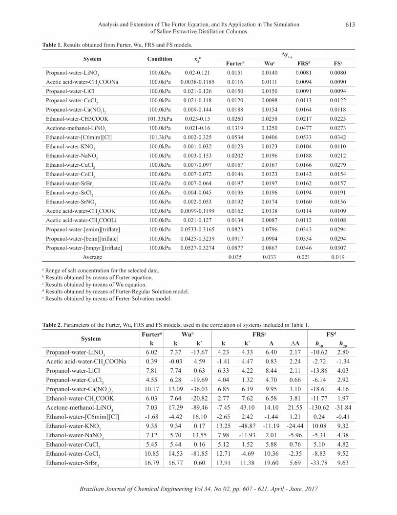
The results of applying Eq. (1), Eq. (3), Eq. (23) and Eq. (38) are reported in Table 1. Correlation of experimental data (Calvar et al., 2007; Peña et al., 1994; Peña et al., 1995; Peña et al., 1996; Vercher et al., 1994; Vercher et al., 1995; Vercher et al., 1996a; Vercher et al., 1996b; Vercher et al., 1999; Vercher et al., 2001; Vercher et al., 2002; Vercher et al., 2003; Vercher et al., 2004a; Vercher et al., 2004b; Vercher et al., 2005; Vercher et al., 2006; Vicent Orchillés et al., 2008; Vicent Orchillés et al., 2011; Zemp and Francesconi, 1992) through the four models was carried out by seeking the parameters that minimized the objective function, defined by:

where N is the number of experimental points, yexp1,s is the

experimental vapour phase mole fraction, and ycal1,s is the

vapour phase mole fraction calculated from yexp1,s = z1/[z1

+ (1 – z1)/αs]. In order to obtain the best parameters from experimental data, the Solver tool of the Microsoft Excel spreadsheet was used to minimize the objective function.

The FRS and FS models yielded better results than the original Furter equation, as was expected since the proposed equations comprise two parameters. In comparison to the two-parameter Wu model (Wu et al., 1999), the FRS and FS models have a better performance in most of the analyzed systems. The average errors for every model show to what extent the models developed in this work improved the correlation of experimental data. The parameters regressed for each model are summarized in Table 2; in particular, parameters for both forms of the FRS model are informed. As can be seen, the restriction of positive values for the solvation parameters at infinite dilution (hi

0) has been relaxed in order to obtain the best OF result (Eq. (39)). A comparison of the curves obtained from each model for the VLE data of the acetone + methanol + lithium nitrate system (Vercher et al., 2006) is depicted in Fig. 1. Both the FRS and FS models yielded the better correlations.

PROCESS SIMULATION

The extended models proposed in this work can be readily incorporated in a simulator of SED columns.

RTln 𝛾𝑖𝑥𝑖 = RTln 𝛾𝑖 ,𝐹𝑥𝑖,𝐹

𝛾𝑖 =𝑥𝑖,𝐹𝑥𝑖

𝛾𝑖 ,𝐹

ln 𝛾𝑖 = ln𝑥𝑖,𝐹𝑥𝑖

+ ln 𝛾𝑖 ,0𝑆𝑅 + ln 𝛾𝑖𝐷𝐻

ln 𝛾1 = ln1− ℎ1𝑧3

𝑧11 + 𝜈3𝑧3

1 + 𝜈3 − ℎ1 − ℎ2 𝑧3+ ln 𝛾1 ,0

𝑆𝑅 + ln 𝛾1𝐷𝐻


𝑧21 + 𝜈3𝑧3

1 + 𝜈3 − ℎ1 − ℎ2 𝑧3+ ln 𝛾2 ,0


ln𝛼𝑠𝛼0

= ln𝛾1 ,𝑠𝑆𝑅𝛾2 ,0

𝑆𝑅

𝛾2,𝑠𝑆𝑅𝛾1,0

𝑆𝑅 =ln𝑥1,𝐹𝑥2𝑥2,𝐹𝑥1

ln𝛼𝑠𝛼0

= ln 1−ℎ1∞𝑧1𝑧3 1−ℎ2∞𝑧2𝑧3⁄


𝑧11 + 𝜈3𝑧3

1 + 𝜈3 − ℎ1 − ℎ2 𝑧3+ ln 𝛾1 ,0



𝑧21 + 𝜈3𝑧3

1 + 𝜈3 − ℎ1 − ℎ2 𝑧3+ ln 𝛾2 ,0


𝑂𝐹 = � 𝑦1,𝑠𝑐𝑎𝑙 − 𝑦1,𝑠

𝑒𝑥𝑝 𝑁⁄𝑛

𝑖=1

= ∆𝑦1,𝑠

(32)

(33)

(34)

(35)

(36)

(37)

(38)

(39)



613

Table 1. Results obtained from Furter, Wu, FRS and FS models.

System Condition x3a

∆y1,s

Furterb Wuc FRSd FSe

Propanol-water-LiNO3 100.0kPa 0.02-0.121 0.0151 0.0140 0.0081 0.0080Acetic acid-water-CH3COONa 100.0kPa 0.0038-0.1185 0.0116 0.0111 0.0094 0.0090Propanol-water-LiCl 100.0kPa 0.021-0.126 0.0150 0.0150 0.0091 0.0094Propanol-water-CuCl2 100.0kPa 0.021-0.118 0.0120 0.0098 0.0113 0.0122Propanol-water-Ca(NO3)2 100.0kPa 0.009-0.144 0.0188 0.0154 0.0164 0.0118Ethanol-water-CH3COOK 101.33kPa 0.025-0.15 0.0260 0.0258 0.0217 0.0223Acetone-methanol-LiNO3 100.0kPa 0.021-0.16 0.1319 0.1250 0.0477 0.0273Ethanol-water-[C6mim][Cl] 101.3kPa 0.002-0.325 0.0534 0.0406 0.0533 0.0342Ethanol-water-KNO3 100.0kPa 0.001-0.032 0.0123 0.0123 0.0104 0.0110Ethanol-water-NaNO3 100.0kPa 0.003-0.153 0.0202 0.0196 0.0188 0.0212Ethanol-water-CuCl2 100.0kPa 0.007-0.097 0.0167 0.0167 0.0166 0.0279Ethanol-water-CoCl2 100.0kPa 0.007-0.072 0.0146 0.0123 0.0142 0.0154Ethanol-water-SrBr2 100.6kPa 0.007-0.064 0.0197 0.0197 0.0162 0.0157Ethanol-water-SrCl2 100.0kPa 0.004-0.045 0.0196 0.0196 0.0194 0.0191Ethanol-water-SrNO3 100.0kPa 0.002-0.053 0.0192 0.0174 0.0160 0.0156Acetic acid-water-CH3COOK 100.0kPa 0.0099-0.1199 0.0162 0.0138 0.0114 0.0109Acetic acid-water-CH3COOLi 100.0kPa 0.021-0.127 0.0134 0.0087 0.0112 0.0108Propanol-water-[emim][triflate] 100.0kPa 0.0533-0.3165 0.0823 0.0796 0.0343 0.0294Propanol-water-[beim][triflate] 100.0kPa 0.0425-0.3239 0.0917 0.0904 0.0334 0.0294Propanol-water-[bmpyr][triflate] 100.0kPa 0.0527-0.3274 0.0877 0.0867 0.0346 0.0307

Average 0.035 0.033 0.021 0.019

a Range of salt concentration for the selected data.b Results obtained by means of Furter equation.c Results obtained by means of Wu equation.d Results obtained by means of Furter-Regular Solution model.e Results obtained by means of Furter-Solvation model.

Table 2. Parameters of the Furter, Wu, FRS and FS models, used in the correlation of systems included in Table 1.

System Furtera Wub FRSc FSd

k k k´ k k´ A ∆A h10 h20

Propanol-water-LiNO3 6.02 7.37 -13.67 4.23 4.33 6.40 2.17 -10.62 2.80Acetic acid-water-CH3COONa 0.39 -0.03 4.59 -1.41 4.47 0.83 2.24 -2.72 -1.34Propanol-water-LiCl 7.81 7.74 0.63 6.33 4.22 8.44 2.11 -13.86 4.03Propanol-water-CuCl2 4.55 6.28 -19.69 4.04 1.32 4.70 0.66 -6.14 2.92Propanol-water-Ca(NO3)2 10.17 13.09 -36.03 6.85 6.19 9.95 3.10 -18.61 4.16Ethanol-water-CH3COOK 6.03 7.64 -20.82 2.77 7.62 6.58 3.81 -11.77 1.97Acetone-methanol-LiNO3 7.03 17.29 -89.46 -7.45 43.10 14.10 21.55 -130.62 -31.84Ethanol-water-[C6mim][Cl] -1.68 -4.42 16.10 -2.65 2.42 -1.44 1.21 0.24 -0.41Ethanol-water-KNO3 9.35 9.34 0.17 13.25 -48.87 -11.19 -24.44 10.08 9.32Ethanol-water-NaNO3 7.12 5.70 13.55 7.98 -11.93 2.01 -5.96 -5.31 4.38Ethanol-water-CuCl2 5.45 5.44 0.16 5.12 1.52 5.88 0.76 5.10 4.82Ethanol-water-CoCl2 10.85 14.53 -81.85 12.71 -4.69 10.36 -2.35 -8.83 9.52Ethanol-water-SrBr2 16.79 16.77 0.60 13.91 11.38 19.60 5.69 -33.78 9.63



Figure 1. Isobaric z'-y diagrams for acetone + methanol + lithium nitrate system (•: experimental data obtained from Vercher et al. ( 2006); – – – –: calculated data using Furter equation; – – –: calculated data using Wu equation; –––: calculated data using FRS model; –––: calculated data using FS model).

Table 2. Cont.

System Furtera Wub FRSc FSd

k k k´ k k´ A ∆A h10 h20

Ethanol-water-SrCl2 17.28 17.28 -0.02 16.04 7.20 19.64 3.60 -29.44 12.01Ethanol-water-SrNO3 10.03 3.39 177.80 13.11 -31.36 -2.57 -15.68 6.77 9.27Acetic acid-water-CH3COOK 2.01 -1.93 48.79 -1.46 7.56 2.32 3.78 -6.00 -1.51Acetic acid-water-CH3COOLi -1.69 -4.60 31.41 -3.15 3.19 -1.55 1.59 -0.04 -3.33Propanol-water-[emim][triflate] 1.45 3.32 -8.02 -2.30 10.39 2.89 5.20 -8.99 -3.37Propanol-water-[beim][triflate] 0.03 1.44 -5.03 -3.69 10.33 1.47 5.16 -7.34 -6.57Propanol-water-[bmpyr][triflate] 0.48 1.49 -4.01 -3.10 9.79 1.80 4.90 -7.32 -5.15

a Parameters obtained for Furter equation.b Parameters obtained for Wu equation.c Parameters obtained for Furter-Regular Solution model.d Parameters obtained for Furter-Solvation model.



615

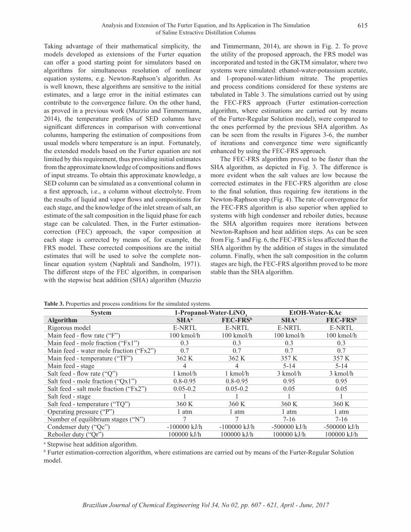
Taking advantage of their mathematical simplicity, the models developed as extensions of the Furter equation can offer a good starting point for simulators based on algorithms for simultaneous resolution of nonlinear equation systems, e.g. Newton-Raphson’s algorithm. As is well known, these algorithms are sensitive to the initial estimates, and a large error in the initial estimates can contribute to the convergence failure. On the other hand, as proved in a previous work (Muzzio and Timmermann, 2014), the temperature profiles of SED columns have significant differences in comparison with conventional columns, hampering the estimation of compositions from usual models where temperature is an input. Fortunately, the extended models based on the Furter equation are not limited by this requirement, thus providing initial estimates from the approximate knowledge of compositions and flows of input streams. To obtain this approximate knowledge, a SED column can be simulated as a conventional column in a first approach, i.e., a column without electrolyte. From the results of liquid and vapor flows and compositions for each stage, and the knowledge of the inlet stream of salt, an estimate of the salt composition in the liquid phase for each stage can be calculated. Then, in the Furter estimation-correction (FEC) approach, the vapor composition at each stage is corrected by means of, for example, the FRS model. These corrected compositions are the initial estimates that will be used to solve the complete non-linear equation system (Naphtali and Sandholm, 1971). The different steps of the FEC algorithm, in comparison with the stepwise heat addition (SHA) algorithm (Muzzio

and Timmermann, 2014), are shown in Fig. 2. To prove the utility of the proposed approach, the FRS model was incorporated and tested in the GKTM simulator, where two systems were simulated: ethanol-water-potassium acetate, and 1-propanol-water-lithium nitrate. The properties and process conditions considered for these systems are tabulated in Table 3. The simulations carried out by using the FEC-FRS approach (Furter estimation-correction algorithm, where estimations are carried out by means of the Furter-Regular Solution model), were compared to the ones performed by the previous SHA algorithm. As can be seen from the results in Figures 3-6, the number of iterations and convergence time were significantly enhanced by using the FEC-FRS approach.

The FEC-FRS algorithm proved to be faster than the SHA algorithm, as depicted in Fig. 3. The difference is more evident when the salt values are low because the corrected estimates in the FEC-FRS algorithm are close to the final solution, thus requiring few iterations in the Newton-Raphson step (Fig. 4). The rate of convergence for the FEC-FRS algorithm is also superior when applied to systems with high condenser and reboiler duties, because the SHA algorithm requires more iterations between Newton-Raphson and heat addition steps. As can be seen from Fig. 5 and Fig. 6, the FEC-FRS is less affected than the SHA algorithm by the addition of stages in the simulated column. Finally, when the salt composition in the column stages are high, the FEC-FRS algorithm proved to be more stable than the SHA algorithm.

Table 3. Properties and process conditions for the simulated systems.System 1-Propanol-Water-LiNO3 EtOH-Water-KAc

Algorithm SHAa FEC-FRSb SHAa FEC-FRSb

Rigorous model E-NRTL E-NRTL E-NRTL E-NRTLMain feed - flow rate (“F”) 100 kmol/h 100 kmol/h 100 kmol/h 100 kmol/hMain feed - mole fraction (“Fx1”) 0.3 0.3 0.3 0.3Main feed - water mole fraction (“Fx2”) 0.7 0.7 0.7 0.7Main feed - temperature (“TF”) 362 K 362 K 357 K 357 KMain feed - stage 4 4 5-14 5-14Salt feed - flow rate (“Q”) 1 kmol/h 1 kmol/h 3 kmol/h 3 kmol/hSalt feed - mole fraction (“Qx1”) 0.8-0.95 0.8-0.95 0.95 0.95Salt feed - salt mole fraction (“Fx2”) 0.05-0.2 0.05-0.2 0.05 0.05Salt feed - stage 1 1 1 1Salt feed - temperature (“TQ”) 360 K 360 K 360 K 360 KOperating pressure (“P”) 1 atm 1 atm 1 atm 1 atmNumber of equilibrium stages (“N”) 7 7 7-16 7-16Condenser duty (“Qc”) -100000 kJ/h -100000 kJ/h -500000 kJ/h -500000 kJ/hReboiler duty (“Qr”) 100000 kJ/h 100000 kJ/h 100000 kJ/h 100000 kJ/h

a Stepwise heat addition algorithm.b Furter estimation-correction algorithm, where estimations are carried out by means of the Furter-Regular Solution model.



Figure 2. Comparison between the SHA (left) and FEC-FRS (right) approach.

Figure 3. Comparison of convergence time for the SHA approach (dark grey columns), and the FEC-FRS approach (light grey columns). Simulated system: 1-Prop-H2O-LiNO3.



617

Figure 4. Comparison of the number of iterations required to achieve convergence, for the SHA approach (dark grey columns), and the FEC-FRS approach (light grey columns). Simulated system: 1-Prop-H2O-LiNO3.

Figure 5. Comparison of convergence time for the SHA approach (dark grey columns), and the FEC-FRS approach (light grey columns). Simulated system: EtOH -H2O-KAc.



CONCLUSIONS

In this work, the Furter equation has been studied and extended by means of the activity models approach. As a result of this analysis, two new models have been proposed as extensions of the Furter equation. These new models retain the simplicity and improve the average deviation of vapor phase mole fraction in comparison to previous models, including another two-parameter model proposed by Wu et al. (1999), even when applied to the entire salt/solvent concentration range. In addition, through the consideration of activity coefficients, the interactions between the different components (volatile and nonvolatile) were included in the model. As a consequence, the relationship between the Furter constant and the proportion of the volatile components arose naturally.

Although the new models developed in this work are an improvement over previous equations, more important is the possibility offered by the activity coefficient approach to be used as a tool to extend the Furter equation toward even more accurate models.

Finally, the Furter extended models have been integrated into a SED column simulator in order to enhance the stability and rate of convergence. Since these models are not affected by the uncertainty in the temperature profile of the distillation column, the vapor compositions at each stage can be corrected from a conventional distillation column to a SED column. As has been proved from the

simulation results of two different systems, the inclusion of Furter extended models into the simulator software led to a more efficient algorithm.

NOMENCLATURE

Aij : parameter of the regular solution model.C,C',C'': constant of integrationfi : fugacity of component i in the liquid phaseGE : molar excess Gibbs free energyh1 : solvation number of salt with component i.Hi: molar enthalpy of component “i”k, k': parameter of the salt effect.nα

i: number of moles “i” in α phase.P: pressure.R: universal constant gas.Si: molar entropy of component “i”.T: temperature.Vi: molar volume of component “i”.xi: liquid phase mole fraction of component “i” based on undissociated species.xia: effective mole fraction of solvent “i” on a salt free basis.yi: vapor phase mol fraction of component “i” in the salt-free system.

1sy∆ : N , N is the number of data

points considered.

Figure 6. Comparison of the number of iterations required to achieve convergence, for the SHA addition approach (dark grey columns), and the FEC-FRS approach (light grey columns). Simulated system: EtOH -H2O-KAc.

( )1, 1,1

ncal exp

s si

y y N=

−∑



619

zi : liquid phase mol fraction for component “i”, on a salt free basis.Greek lettersα : relative volatility β : 1/(1+z3) : fugacity coefficient of the component i in the mixture. : activity coefficient for the solvent i : chemical potencial of component “i” in the α phase. : derivative of chemical potential of component “i” with respect to “j” component in the α phase.v3 : electrolyte stoichiometric coefficient.σ : saline coefficient.SubscriptsF : free molecules : system with salt+ : property of the more volatile component 0 : salt-free system1,2 : volatile components3 : non-volatile component (salt or ionic-liquid)SuperscriptsLR : long-range.SR : short-range.∞ : infinite dilution of the salt° : pure component

REFERENCES

Bastos, P.D.A., Oliveira, F.S., Rebelo, L.P.N., Pereiro, A.B., Marrucho, I.M., Separation of azeotropic mixtures using high ionicity ionic liquids based on 1-ethyl-3-methylimidazolium thiocyanate. Fluid Phase Equilibria, 389, p. 48–54 (2015).

Calvar , N., González, B., Gómez, E., Domínguez, A., Study of the behaviour of the azeotropic mixture ethanol–water with imidazolium-based ionic liquids. Fluid Phase Equilibria, 259, p. 51–56 (2007).

Cardoso, M. and O’Connell, J., Activity coefficients in mixed solvents electrolyte solutions. Fluid Phase Equilibria, 33, p. 315–326 (1987).

Chen, C.C., Song Y., Generalized electrolyte-NRTL model for mixed-solvent electrolyte systems, AIChE Journal, 50, p. 1928-1941 (2004).

Gmehling, J., Present status and potential of group contribution methods for process development. The Journal of Chemical Thermodynamics, 41, p. 731–747 (2009).

Hashitani, M. and Hirata, M., Salt effect in vapor-liquid equilibrium - acetic ester-alcohol with potassium acetate and zinc chloride -. Journal of Chemical Engineering of Japan, 2, p. 149-153 (1969).

Iliuta, M. C., Thomsen, K., Rasmussen, P., Extended UNIQUAC model for correlation and prediction of vapour-liquid-solid equilibria in aqueous salt systems containing non-electrolytes. Part A. Methanol-water-salt systems. Chemical Engineering Science 55, p. 2673-2686 (2000).

Jaques, D. and Furter, W.F., Effect of a dissolved salt on vapor-liquid equilibrium with liquid composition held constant. Industrial & Engineering Chemistry Fundamentals, 13, p. 238-241 (1974).

Johnson, A.I. and Furter., W.F., Salt effect in vapour-liquid equilibrium, Part II. The Canadian Journal of Chemical Engineering, 38, p. 78-87 (1960).

Kablukov, I.A. Zhurnal Fizicheskoi Khimii – Khimii Obshchei, 23, p. 388 (1891) (from Furter and Cook (1967))

Kiss, A.A. and Suszwalak, D.J.P.C. Enhanced bioethanol dehydration by extractive and azeotropic distillation in dividing-wall columns. Separation and Purification Technology, 86, p. 70–78 (2012).

Li, J., Polka, H.M., Gmehling, J., A gE model for single and mixed solvent electrolyte systems. 1. Model and results for strong electrolytes. Fluid Phase Equilibria, 94, p. 89–114 (1994).

Llano-Restrepo, M. and Aguilar-Arias, J., Modeling and simulation of saline extractive distillation columns for the production of absolute ethanol. Computers and Chemical Engineering, 27, p. 113-121 (2003).

Loehe, J.R. and Donohue, M.D., Recent advances in modeling thermodynamic properties of aqueous strong electrolyte systems. AIChE Journal, 43, p. 180-195 (1997).

Matsuda, H. , Takahara, H., Fujino, S., Constantinescu, D., Kurihara, K., Tochigi, K., Ochi, K., Gmehling, J., Selection of entrainers for the separation of the binary azeotropic system methanol + dimethyl carbonate by extractive distillation. Fluid Phase Equilibria, 310, p. 166– 181 (2011).

Meranda D. and Furter, W.F., Vapor-liquid equilibrium in alcohol-water systems containing disolved acetate salts. AIChE Journal, 17, p. 38-42 (1971).

Miller,W.L., On the second differential coefficients of Gibbs’ function ζ. The vapour tensions, freezing and boiling points of ternary mixtures. The Journal Physical Chemistry, 1, p. 633 (1897) (from Johnson and Further, 1960)

Mock, B., Evans, L.B., Chen, C.C., Thermodynamic representation of phase equilibria of mixed-solvent electrolyte systems. AIChE Journal, 32, p. 1655-1664 (1986).

Mohs, A., Gmehling, J., A revised LIQUAC and LIFAC model (LIQUAC*/LIFAC*) for the prediction of

iφ

iγiαµ

ijαµ



properties of electrolyte containing solutions. Fluid Phase Equilibria, 337, p. 311– 322 (2013)

Muzzio, C.R. and Timmermann, E.O., Effect of electrolytes on the temperature profile of saline extractive distillation columns. Latin American Applied Research, 44, p. 41-46 (2014).

Naphtali, L. M. and Sandholm, D. P., Multicomponent separation calculations by linearization. AIChE Journal, 17, p. 148–153 (1971).

Nothnagel, K.H., Abrams, D.S., Prausnitz, J.M., Generalized correlation for fugacity coefficients in mixtures at moderate pressures. Industrial & Engineering Chemical Process Design and Development, 12, p. 25–35 (1973).

Peña, M. P., Vercher, E., Martinez-Andreu, A., Isobaric vapor-liquid equilibrium for ethanol + water + sodium nitrate. Journal of Chemical & Engineering Data, 41, 1097-1100 (1996).

Peña, M. P., Vercher, E., Martinez-Andreu, A., Isobaric vapor-liquid equilibrium for ethanol + water + cobalt(ii) chloride. Journal of Chemical & Engineering Data, 39, p. 763-766 (1994).

Peña, M. P., Vercher, E., Martinez-Andreu, A., Isobaric vapor-liquid equilibrium for ethanol + water + strontium chloride. Journal of Chemical & Engineering Data, 40, p. 311-314 (1995).

Pereiro, A.B., Araújo, J.M.M., Esperança, J.M.S.S., Marrucho, I.M., Rebelo, L.P.N., Ionic liquids in separations of azeotropic systems – A review. The Journal of Chemical Thermodynamics, 46, p. 2–28 (2012).

Pinto, R.T.P., Wolf-Maciel, M.R., Lintomen, L., Saline extractive distillation process for ethanol purification. Computers and Chemical Engineering 24, p. 1689-1694 (2000).

Prigogine, I. and Defay, R., Chemical Themodynamics, Longmans Green and Co. Ltd., London (1954).

Robinson, R.A. and Stokes, R.H, Electrolyte Solutions, 2nd. ed. Butterworths, London (1959).

Sander, B., Fredenslund, A., Rasmussen, P., Calculation of vapour-liquid equilibria in mixed solvent/salt systems using an extended Uniquac equation. Chemical Engineering Science, 41, p. 1171-1183 (1986).

Tassios, D. P., Rapid screening of extractive distillation solvents. In: R.F. Gould, Extractive and azeotropic distillation, Advances in Chemistry Series 115, p. 46-63 (1972).

Vercher, E. , Orchillés, A. V., Miguel, P- J., González-Alfaro, V., Martínez-Andreu, A., Isobaric vapor–liquid equilibria for acetone + methanol + lithium nitrate at 100 kPa. Fluid Phase Equilibria, 249, p. 97–103 (2006).

Vercher, E., Peña, M. P., Martinez-Andreu, A., Isobaric vapor-liquid equilibrium for ethanol + water +

potassium nitrate. Journal of Chemical & Engineering Data, 41, p. 66-69 (1996a).

Vercher, E., Peña, M. P., Martinez-Andreu, A., Isobaric vapor-liquid equilibrium for ethanol + water + copper(ii) chloride. Journal of Chemical & Engineering Data, 40, p. 657-661 (1995).

Vercher, E., Peña, M. P., Martinez-Andreu, A., Isobaric vapor-liquid equilibrium data for the ethanol + water + strontium bromide system. Journal of Chemical & Engineering Data, 39, p. 316-319 (1994).

Vercher, E., Peña, M. P., Martinez-Andreu, A., Isobaric vapor-liquid equilibrium for ethanol + water + strontium nitrate. Journal of Chemical & Engineering Data, 41, p. 748-751 (1996b).

Vercher, E., Rojo, F. J., Martínez-Andreu, A., Isobaric vapor-liquid equilibria for 1-propanol + water + calcium nitrate. Journal of Chemical & Engineering Data, 44, p. 1216-1221 (1999).

Vercher, E., Vázquez, M. I., Martínez-Andreu, A., Isobaric vapor-liquid equilibria for 1-propanol + water + lithium nitrate at 100 kPa. Fluid Phase Equilibria, 202, p. 121–132 (2002).

Vercher, E., Vázquez, M. I., Martínez-Andreu, A., Isobaric vapor-liquid equilibria for water + acetic acid + sodium acetate. Journal Chemical & Engineering Data, 48, p. 217-220 (2003).

Vercher, E., Vázquez, M. I., Martínez-Andreu, A., Isobaric vapor-liquid equilibrium for water + acetic acid + lithium acetate. Journal of Chemical & Engineering Data, 46, p. 1584-1588 (2001).

Vercher, E., Vicent Orchillés, A., González-Alfaro, V., Martínez-Andreu, A., Isobaric vapor–liquid equilibria for 1-propanol +water + copper(II) chloride at 100 kPa. Fluid Phase Equilibria, 227, p. 239–244 (2005).

Vercher, E., Vicent Orchillés, A., Vázquez, M. I., Martínez-Andreu, A., Isobaric vapor–liquid equilibria for 1-propanol + water + lithium chloride at 100 kPa. Fluid Phase Equilibria, 216, p. 47–52 (2004a).

Vercher, E., Vicent Orchillés, A., Vázquez, M. I., Martínez-Andreu, A., Isobaric vapor-liquid equilibrium for water + acetic acid + potassium acetate. Journal of Chemical & Engineering Data, 49, p. 566-569 (2004b).

Vicent Orchillés, A., Miguel, P. J., González-Alfaro, V., Vercher, E., Martínez-Andreu, A., Isobaric vapor-liquid equilibria of 1-propanol + water + acetic acid + trifluoromethanesulfonate-based ionic liquid ternary systems at 100kPa. Journal of Chemical & Engineering Data, 56, p. 4454–4460 (2011).

Vicent Orchillés, A., Miguel, P. J., Vercher, E., Martínez-Andreu, A., Isobaric vapor-liquid equilibrium for 1-propanol + water + acetic acid + 1-ethyl-3-methylimidazolium trifluoromethanesulfonate at



621

100kPa. Journal of Chemical & Engineering Data, 53, p. 2426–2431 (2008).

Wu, W.L., Zhang, Y.M., Lu, X.H., Wang, Y.R., Shi, J., Lu, Benjamin C.-Y., Modification of the Furter equation and correlation of the vapor–liquid equilibrium for mixed-solvent electrolyte systems. Fluid Phase Equilibria, 154, p. 301-310 (1999).

Wu, Y.G., Tabata, M., Takamuku, T., Yamaguchi, A., Kawaguchi, T., Chung, N.H., An extended Johnson–Furter equation to salting-out phase separation of

aqueous solution of water-miscible organic solvents. Fluid Phase Equilibria, 192, p. 1–12 (2001).

Zemp, R. J. and Francesconi, A. Z., Salt effect on phase equilibria by a reclrculating still. Journal of Chemical & Engineering Data, 37, p. 313-316 (1992).

Zhang, Z., Hu, A., Zhang, T., Zhang, Q., Sun, M., Sun, D., Li, W., Separation of methyl acetate + methanol azeotropic mixture using ionic liquids as entrainers, Fluid Phase Equilibria, 401, p. 1–8 (2015).

Documents

ANALYSIS AND EXTENSION OF THE FURTER EQUATION, AND …relative volatility. This approach allowed systematic extensions of the Furter equation and a brief review of the theoretical