Embed Size (px)
Citation preview

Analysis and Evaluation of Register Transfer Logic
Software Defined Radio Performance
WPI – MIT Lincoln Laboratory A Major Qualifying Project
Submitted to the faculty of the
WORCESTER POLYTECHNIC INSTITUTE
in partial fulfillment of the requirements for the
Degree of Bachelor of Science
in Electrical and Computer Engineering
by
____________________________________
Krishna (Dylan) Mahalingam
Date: October 11, 2016
____________________________________
Stephen Michelini
Date: October 11, 2016
Approved: ____________________________________
Edward A. Clancy, Faculty Advisor, WPI
Date: October 11, 2016
This work is sponsored by the Department of the Air Force under Air Force Contract
#FA8702-15-D-0001. Opinions, interpretations, conclusions, and recommendations are
those of the authors and not necessarily endorsed by the United States Government.

2
Abstract
When determining the capabilities of adversaries, it is important to consider what
they can do with relatively inexpensive technology. The Register Transfer Logic
Software Defined Radio (RTL-SDR) is a low-cost software-defined radio (SDR) built
around a television tuner, which is actively supported by the open-source community
for use as a radio receiver. Group 108 at MIT Lincoln Laboratory has interest in
determining the potential capabilities of SDR receivers for air surveillance. Several RTL-
SDRs were put through various tests to compare their performance characteristics to
those of the Ettus Universal Software Radio Peripheral (USRP), a more expensive
commercial SDR. These tests have shown that a standalone RTL-SDR could be a
suitable replacement for a USRP within a reception frequency range of 50-1600 MHz at
a sample rate no higher than 2.85 MHz. The RTL-SDRs have notably good performance,
despite more limitations when compared to the Ettus USRP. Prototypes were built for
both a two-channel and three-channel clock-synchronized RTL-SDR system; these
systems were tested for phase offset between their receiver channels. Further work can
be done to implement multi-channel RTL-SDR systems for geolocation or wideband
signal reception purposes. RTL-SDRs cannot compete directly on performance with
more expensive SDRs specifically built for reception, but since they show good
performance for their price and can be utilized in a multi-channel receiver, they are
worth continuing to research in the future.

3
Statement of Authorship
Over the course of a summer internship at MIT Lincoln Laboratory, Dylan
completed certain portions of the performance testing of the received sample ratio and
noise floor characteristics, as detailed in Sections 3.3 and 3.4. Both group members
contributed equally to all other components of the project during the formal project
period.
Both group members contributed to the editing and revision of all sections of the
report, but sections were originally written as specified below:
Dylan Mahalingam: Sections 2.3, 2.4, 3.1.1, 3.2, 3.3, 3.4, 3.5, 3.6
Stephen Michelini: Sections 2.1, 2.2, 2.5, 2.6, 3.1.2, 3.7, 3.8, 3.9, 3.10, 3.11
Both Team Members: Abstract, Executive Summary, and all other sections and chapters

4
Acknowledgements
We would like to express our sincerest gratitude to Sarah Curry, Lisa Basile, Chris
Massa, Matt Beals, and Vito Mecca, our supervisors and mentors at MIT Lincoln
Laboratory. Their continued support and assistance throughout the duration of the
project was invaluable.
We also thank Professor Edward Clancy, our WPI faculty advisor, for providing
valuable feedback on our project and report, regularly attending meetings with our
team, and always challenging us to improve.
Special thanks go to Sarah Curry, Katie Haas, Seth Hunter, and Emily Anesta for
coordinating the MIT Lincoln Laboratory MQP program, and to Jim Burke, Bob
Giovannucci, Andrew Daigle, Dave McQueen, John Palmer, Jeremy VanSchalkwyk, and
Michael Stillwell for all of their contributions to our work.

5
Table of Contents
Abstract ................................................................................................................... 2
Statement of Authorship ............................................................................................ 3
Acknowledgements ................................................................................................... 4
Table of Contents...................................................................................................... 5
Table of Figures ........................................................................................................ 8
Table of Tables ....................................................................................................... 11
Executive Summary ................................................................................................. 13
1.0 Introduction ...................................................................................................... 18
2.0 Background ...................................................................................................... 20
2.1 Software Defined Radios ................................................................................. 20
2.2 ADS-B Signals ................................................................................................ 20
2.3 SDR Models ................................................................................................... 22
2.3.1 The RTL-SDR ........................................................................................... 22
2.3.2 The USRP as Compared to the RTL-SDR .................................................... 23
2.4 SDR Performance Characteristics ..................................................................... 24
2.4.1 Received Sample Ratio ............................................................................. 24
2.4.2 Noise Floor .............................................................................................. 25
2.4.3 Noise Figure ............................................................................................. 26
2.4.4 Center Frequency ..................................................................................... 26
2.5 Radar Range Equation .................................................................................... 28
2.6 Multi-Channel RTL-SDR System ....................................................................... 28
2.6.1 Synchronized-Clock System ....................................................................... 29
2.6.2 Clock Stability and Clock Jitter ................................................................... 29

6
2.6.3 Phase of Receivers ................................................................................... 30
3.0 Methods and Results ......................................................................................... 32
3.1 Equipment Used ............................................................................................. 32
3.1.1 Hardware ................................................................................................. 32
3.1.2 Software .................................................................................................. 33
3.2 Analog-to-Digital Converter Unit Calibration ..................................................... 34
3.3 Received Sample Ratio Performance Testing .................................................... 38
3.3.1 Methods .................................................................................................. 38
3.3.2 Results .................................................................................................... 39
3.4 Noise Floor Performance Testing ..................................................................... 41
3.4.1 Methods .................................................................................................. 41
3.4.2 Results .................................................................................................... 41
3.5 Noise Figure Performance Testing ................................................................... 43
3.5.1 Methods .................................................................................................. 43
3.5.2 Results .................................................................................................... 44
3.6 Frequency Coverage Performance Testing ....................................................... 48
3.6.1 Methods .................................................................................................. 48
3.6.2 Results .................................................................................................... 49
3.7 RTL-SDR Clock Stability Measurement ............................................................. 51
3.7.1 Methods .................................................................................................. 52
3.7.2 Results .................................................................................................... 53
3.8 Two-Channel RTL-SDR System Build ............................................................... 54
3.9 Two-Channel RTL-SDR System Phase Testing .................................................. 57
3.9.1 Rise Time Delay Methods .......................................................................... 57

7
3.9.2 Rise Time Delay Results ............................................................................ 60
3.9.3 Reception Stability Methods ...................................................................... 61
3.9.4 Reception Stability Results ........................................................................ 63
3.9.5 Increased Frequency of Injected Signal Methods ........................................ 67
3.9.6 Increased Frequency of Injected Signal Results .......................................... 68
3.10 Three-Channel RTL-SDR Build ....................................................................... 69
3.11 Three-Channel RTL-SDR Reception Stability ................................................... 72
3.11.1 Reception Stability Methods .................................................................... 72
3.11.2 Reception Stability Results ...................................................................... 74
4.0 Discussion......................................................................................................... 77
5.0 Conclusion ........................................................................................................ 84
Works Cited ............................................................................................................ 86

8
Table of Figures
Figure 1 – Average Received Magnitude of -20-dBm CW Signal at Various Center
Frequencies .................................................................................................. 16
Figure 2 – Diagram of ADS-B Showing How Aircraft Can Use GPS Signals and Send
These Data to a Ground Station (Smyrna Air Center, Inc.) ............................... 21
Figure 3 – Example Frequency Domain Plot of a Signal with a Center Frequency of 9
MHz ............................................................................................................. 27
Figure 4 - Measuring Time Interval Error of Edge with One Ideal Clock Signal and One
Actual Clock Signal (SiTime Corporation, 2014) ............................................... 30
Figure 5 – Three RTL-SDR models. SQdeal RTL-SDR, RTL-SDR Blog RTL-SDR, and
NooElec RTL-SDR, from Top to Bottom. ......................................................... 33
Figure 6 – ADC Unit Calibration Hardware Setup ....................................................... 35
Figure 7 - RTL-SDR Volt Conversion Factor Vs. dBm at Input ..................................... 36
Figure 8 - USRP Volt Conversion Factor Vs. dBm at Input .......................................... 37
Figure 9 – Received Sample Ratio Testing Hardware Setup ........................................ 39
Figure 10 - Received Sample Ratio ........................................................................... 40
Figure 11 - Noise Floor Testing Hardware Setup ....................................................... 41
Figure 12 - Noise Floor (Line Terminated)................................................................. 42
Figure 13 - Noise Floor (Line Unterminated) ............................................................. 42
Figure 14 - Recorded Power vs. Input Power Calibration Curves ................................ 45
Figure 15 - Output SNR vs. Input SNR Calibration Curve (RTL-SDR Blog 1) ................. 46
Figure 16 - Output SNR vs. Input SNR Calibration Curve (USRP) ................................ 47
Figure 17 – CW Frequency Coverage Testing Hardware Setup ................................... 48
Figure 18 - Wideband Frequency Coverage Testing Hardware Setup .......................... 49
Figure 19 - Average Received Magnitude of -20-dBm CW Signal at Various Center
Frequencies .................................................................................................. 50
Figure 20 - Wideband Frequency Response at Center Frequency of 1090 MHz ............ 51
Figure 21 – SQdeal RTL-SDR Top ............................................................................. 54

9
Figure 22 - SQdeal RTL-SDR Bottom ........................................................................ 54
Figure 23 – Modified Two-Channel RTL-SDR. Upper RTL-SDR with Oscillator Removed.
Connection Soldered to Oscillator on Lower RTL-SDR. ..................................... 55
Figure 24 – Modified Two-Channel RTL-SDR. Upper RTL-SDR Oscillator Soldered to
Lower RTL-SDR. ........................................................................................... 56
Figure 25 – Modified Two-Channel RTL-SDR with Casing ........................................... 56
Figure 26- Two-Channel Phase Testing Hardware Setup ............................................ 58
Figure 27 - Time Lag of Two-Channel RTL-SDR System without Time Correction ........ 59
Figure 28 – Enlarged Portion of Figure 27 Showing when RTL-SDR 2 Comes on with
Respect to RTL-SDR 1 ................................................................................... 59
Figure 29 - Phase Lag of Two-Channel RTL-SDR System w/ Phase Correction for First
Sample Reception ......................................................................................... 60
Figure 30- Two-Channel Reception Stability Setup with Signal Generator at 895.05 MHz
.................................................................................................................... 62
Figure 31 - 50 kHz Wave Received by the Two-Channel RTL-SDR System Filtered by a
Band-Pass Filter ............................................................................................ 62
Figure 32 - Histogram of Test 2 of the Time Error for the Two-Channel RTL-SDR System
with Signal Generator at 895.05 MHz ............................................................. 65
Figure 33 - Two-Channel Reception Stability Setup with Signal Generator at 895.10 MHz
.................................................................................................................... 68
Figure 34 - NooElec RTL-SDR Top ............................................................................ 69
Figure 35 - NooElec RTL-SDR Bottom ....................................................................... 69
Figure 36 - NooElec RTL-SDR Top View Driving the Three-Channel System ................ 70
Figure 37 - NooElec RTL-SDR Bottom View Driving the Three-Channel System ........... 71
Figure 38 – Three-Channel RTL-SDR System with Casing .......................................... 72
Figure 39 - Three-Channel RTL-SDR Reception Stability Hardware Setup .................... 73
Figure 40 - 50 kHz Wave Received by the Three-Channel RTL-SDR System Filtered by a
Band-Pass Filter ............................................................................................ 75
Figure 41 - Histogram of Peak Location Time Error in Three-Channel System Receiving
an 895.05 MHz wave ..................................................................................... 76

10
Figure 42 - Receiver SNR as a Function of Radar Range with High-Strength ADS-B
Transmitter................................................................................................... 80
Figure 43 - Receiver SNR as a Function of Radar Range with Low-Strength ADS-B
Transmitter................................................................................................... 80

11
Table of Tables
Table 1 - Two-Channel RTL-SDR Reception Stability Phase Results ............................ 17
Table 2 - Overview of General Specifications for SDR Grades ..................................... 19
Table 3 - ADS-B Signal Transmit Powers (International Civil Aviation Organization,
2007) ........................................................................................................... 21
Table 4 - RTL-SDR Tuners and Frequency Ranges (About RTL-SDR, 2013) ................ 23
Table 5 - USRP and RTL-SDR Comparison ................................................................ 24
Table 6 – Volt Conversion Factors ............................................................................ 38
Table 7 - Noise Figure Calculated by 3-dB Increase from Noise Floor ......................... 45
Table 8 - Noise Figure Calculated by Offset between Input and Output SNR ............... 47
Table 9 – Results from Time Interval Error Test ........................................................ 53
Table 10 - Results from the Clock Frequency Test ..................................................... 53
Table 11 – Two-Channel RTL-SDR System Time Delays ............................................. 61
Table 12 - Time Difference over 50 ms of Two-Channel Multi-RTL System with a Signal
Generator Operating at 895.05 MHz ............................................................... 64
Table 13 - Comparison of Interpolated Data Vs. Data with No Interpolation................ 64
Table 14 - Phase Difference over 50 ms of Two-Channel Multi-RTL System with a Signal
Generator Operating at 895.05 MHz(f=50kHz) ................................................ 67
Table 15 - Time Difference over 50 ms of Two-Channel Multi-RTL System with a Signal
Generator Operating at 895.10 MHz ............................................................... 68
Table 16 - Phase Difference over 50 ms of Two-Channel RTL-SDR System with a Signal
Generator Operating at 895.10 MHz (f = 100 kHz) .......................................... 68
Table 17 – Mean Time Difference of Signal Detected by Three-Channel RTL-SDR System
.................................................................................................................... 74
Table 18 – Standard Deviation Time Difference of Signal Detected by Three-Channel
RTL-SDR System ........................................................................................... 74
Table 19 - Mean Phase Difference of Signal Detected by Three-Channel RTL-SDR
System ......................................................................................................... 75

12
Table 20 - Standard Deviation of Phase Difference of Signal Detected by Three-Channel
RTL-SDR System ........................................................................................... 75

13
Executive Summary
The objective of this project was to determine the performance characteristics of
the hobbyist-level Register Transfer Logic Software Defined Radios (RTL-SDRs) as
compared to the commercial-level Ettus Universal Software Radio Peripheral (USRP).
After determining the performance characteristics of RTL-SDRs, a multi-channel RTL-
SDR system prototype was developed and tested. This project was carried out for
Group 108 at MIT Lincoln Laboratory. Group 108 works on air defense issues such as
air vehicle survivability, vulnerability of United States Air Force aircraft to weapons
systems, electronic countermeasures, and air surveillance for homeland defense. Group
108 is interested in how a standalone RTL-SDR may be used for air surveillance, and
how the device’s capabilities may be expanded in a multi-channel system.
Software defined radios (SDRs) are radios with some of a typical radio’s
hardware components controlled by software instead. SDRs enable easy changes of
certain parameters such as gain, sample rate, center frequency, and digital signal
processing without requiring any hardware modifications. Two types of SDRs were used
in the project: RTL-SDRs and the USRP. RTL-SDRs are hobbyist radios with DVB-T
television tuners on a USB dongle that are used by the open-source community as
general-purpose SDR receivers. The USRP X310 is a commercial device produced by
Ettus Research.
The USRP X310 is a well-known device that is often used for research and
testing purposes. The USRP X310 costs approximately $6,000 (Ettus Research, 2016).
RTL-SDRs have a smaller form factor and are much less expensive at approximately
$20, but their performance specifications are not well documented and are expected to
be poorer. This project initially focused on comparing the performance of RTL-SDRs to
the performance of a USRP to see how the inexpensive devices compare against a well-
established SDR. There are several major device parameters that were tested on each
standalone device: received sample ratio, noise floor, noise figure, and frequency
coverage. Since it is known that the USRP has a larger sample rate range, a larger

14
reception frequency range, and generally more configurable parameters, all
performance testing was done within the parameter range of the RTL-SDRs.
The sample rate of an SDR is the rate at which the device collects samples
(individual points of data) from an input signal during analog-to-digital conversion. The
received sample ratio of an SDR is the number of samples that are received (as
opposed to being dropped) per the total number of samples that should have been
received over a given period of time. After testing, it was determined that the USRP
maintains a perfect received sample ratio across the RTL-SDR sample rate range of 2.0-
3.2 MHz. The RTL-SDRs maintain a steady received sample ratio up through a sample
rate of 2.85 MHz, but drop samples significantly once above this sample rate. The RTL-
SDRs match USRP performance in terms of received sample ratio up to a sample rate of
2.85 MHz, but not beyond. The RTL-SDRs do meet their advertised requirements for
received sample ratio, though, as they are reported to be operational up through a
sample rate of 3.2 MHz, but they are only guaranteed to not drop samples up through
2.8 MHz.
The noise floor of an SDR is a metric to characterize how much noise, or
undesired signal content, is introduced into the system by the device itself. The
hardware components within a device will introduce a certain amount of noise to the
system. The noise floor is generally considered to be the magnitude of reception from
an SDR when the input is terminated. Testing of the noise floor concluded that the RTL-
SDRs have a very consistent noise floor of about -60 dBm, both across frequencies and
across each device. The USRP, however, has a much lower noise floor of about -85
dBm, so the USRP has much better noise floor performance than the RTL-SDR.
Noise figure is another metric to characterize the noise introduced into a system
by the system itself. The signal-to-noise ratio (SNR) of a device is defined as the
magnitude of the desired signal divided by the magnitude of the noise floor around the
desired signal. Because of noise introduced to an input signal by hardware components
of a device, the SNR of the signal at the input will be greater than the SNR at the

15
output. Noise figure is a quantity describing the relationship between the SNR at the
input of a system as compared to the SNR at the output of the same system (Agilent
Technologies, 2010). The advertised noise figure for the USRP is 8 dB (Ettus Research,
2016). There is no advertised noise figure for RTL-SDRs, but members of the hobbyist
radio community have determined noise figure values ranging from 13.6 dB to 17 dB
(RTL-SDR Blog, 2015). Testing found noise figure values that were inconsistent with
these specifications. One method of testing found a USRP noise figure of 12 dB and
RTL-SDR noise figures ranging from 20 dB to 24 dB. Another method of testing found a
USRP noise figure of 23 dB and RTL-SDR noise figures ranging from 50 dB to 52 dB.
Since these results are inconsistent between the two test methods and inconsistent with
expectations, they are not yet credible.
Although signals are commonly viewed in the time domain, it is often more
useful to analyze a signal in the frequency domain. Testing was done on the SDRs to
characterize how the consistency of the gain of both a continuous-wave (CW) signal
and a bandlimited white noise signal of 50-kHz bandwidth when received at various
frequencies across the RTL-SDRs center frequency range of 24–1766 MHz. The results
of this test can be seen in Figure 1. Testing revealed that the USRP receives an input
signal across the relevant frequency range, with about a 10-dB drop in reception across
a frequency range of 50–450 MHz. The RTL-SDRs receive the input signal across their
frequency range, but have significant drops in reception at the ends of their frequency
range. For many RTL-SDRs, the received signal was at the level of the noise floor at
frequencies below 50 MHz and above 1600 MHz. For each SDR in this test, all CW and
wideband input signals received above the noise floor were received with the correct
bandwidth.

16
Figure 1 – Average Received Magnitude of -20-dBm CW Signal at Various
Center Frequencies
The second major focus of the project was the development and testing of a
multi-channel RTL-SDR system. A two-channel RTL-SDR system was built by connecting
the oscillator of one RTL-SDR to the oscillator input of another RTL-SDR. The system
was verified by collecting data samples from both devices simultaneously.
Initial testing was done on this two-channel system with the receiver inputs of
both devices receiving the same signal from a signal generator via a splitter, to
determine the time difference between the data streams. Both devices were identically
configured and set to immediately start receiving samples. It was determined that the
startup time for the RTL-SDRs to begin receiving samples varied from test to test. The
USB connection that was used to transmit the collected samples from the receiver to
the computer also introduced an unknown delay. These results show that if this multi-
channel system were to be used in an application where synchronization mattered, the
channels would have to be synchronized through software at the start of each data
collection.

17
The next part of the testing for the two-channel RTL-SDR was phase testing.
This test had both devices connected to the same signal generator and each received a
sine wave at 895.05 MHz while receiving at a center frequency of 895 MHz. This offset
gave each RTL-SDR an approximately 50-kHz sine wave after the wave from the signal
generator was down converted to baseband. Sine wave peak locations during a 50-ms
segment were compared between devices. These results show the phase difference
between the devices in various tests.
Table 1 - Two-Channel RTL-SDR Reception Stability Phase Results
Test #
Mean of Phase Difference
Std. Dev. of Phase Difference
Mean of Time Difference
Std. Dev. Of Time Difference
1 4.86 degrees 5.76 degrees 270.27 ns 320.08 ns
2 -4.01 degrees 5.57 degrees -222.78 ns 309.78 ns
3 1.43 degrees 5.75 degrees 79.579 ns 319.57 ns
4 1.66 degrees 4.94 degrees 92.151 ns 274.55 ns
5 -5.37 degrees 5.25 degrees -298.18 ns 292.09 ns
6 3.11 degrees 5.11 degrees 173.32 ns 284.10 ns
After successfully testing the two-channel RTL-SDR system, a three-channel RTL-
SDR system was built and tested. A reception stability test for the phase of the three-
channel system was completed. The three-channel system had similar phase differences
as the two-channel system with a standard deviation of phase difference of around 6
degrees.
This project was able to successfully determine some of the performance
characteristics of RTL-SDRs and compare them to the USRP. As expected, the USRP
outperformed the RTL-SDRs in most of the tests; however, depending on the
requirements of a certain situation, the RTL-SDR may be a suitable receiver. Two-
channel and three-channel RTL-SDR systems were built and tested. With further work
put into signal processing and software synchronization of the devices in these multi-
channel receiver systems, it is possible that such a system could improve upon the
functionality of a standalone RTL-SDR.

18
1.0 Introduction
Software-defined radios (SDRs) are a newer version of the traditional radio
where some hardware components are controlled by software. SDRs have a distinct
advantage over traditional radio equipment because they can easily be reprogrammed.
This feature enables an SDR to have its software modules modified to accommodate
changes such as a new center frequency, whereas a standard radio would require a
physical change of hardware components to modify such parameters. This adaptability
is especially important in the world today because communication systems are always
changing and radios need to be able to suit new needs quickly and effectively. In
addition, this feature adds new functionality such as cognitive radio.
A real-world application for SDRs that can be examined is aircraft surveillance.
According to the Federal Aviation Association, aircraft emit a radio signal called
Automatic Dependent Surveillance-Broadcast (ADS-B), which provides information
about the aircraft to receivers. It is designed to use GPS to locate the aircraft and then
broadcast that position (Federal Aviation Administration, 2016).
SDR usage for air surveillance is an important topic to the sponsor of the project,
MIT Lincoln Laboratory’s Group 108, Tactical Defense Systems. MIT Lincoln Laboratory
is a federally funded research and development center established in 1951. Stationed
on Hanscom Air Force Base, MIT Lincoln Laboratory puts heavy emphasis on its key
mission of air, missile, and maritime defense technology (MIT Lincoln Laboratory).
Group 108 has a strong focus in understanding and analyzing the vulnerabilities of
current U.S. Air Force aircraft, which makes air surveillance a point of interest (MIT
Lincoln Laboratory, 2016).
There are different grades of SDRs on the market, including military-grade,
commercial, and hobbyist devices. A brief overview of some general characteristics for
these grades of SDRs can be found in Table 2.

19
Table 2 - Overview of General Specifications for SDR Grades
Military-Grade Commercial Hobbyist
Performance High Moderate ?
Availability Export-Controlled COTS COTS
Price High Medium Low
Military-grade SDRs are expected to have the highest level of performance, but
their availability is limited and they can be quite expensive. They are also harder to
acquire than commercial SDRs because they are typically export-controlled. Commercial
SDRs have lower performance than military-grade SDRs, but they are much more
common because they are commercially available. Hobbyist SDRs are also highly
available; however, their performance characteristics are generally unknown and
expected to be poorer than commercial radios. If the performance of the less expensive
hobbyist SDRs is sufficient in certain applications, the commercial SDRs can be replaced
by the hobbyist SDRs in that application.
The purpose of this project was to test and characterize the performance of an
inexpensive hobbyist SDR class, the Register Transfer Logic Software Defined Radios
(RTL-SDRs), for applications in air surveillance. The performance specifications of the
RTL-SDRs are compared against the performance specifications of a commercial SDR,
the Ettus Universal Software Radio Peripheral (USRP). In addition, this project involved
the development and testing of a multi-channel RTL-SDR system in an effort to
demonstrate the capabilities of the RTL-SDR for air surveillance purposes.

20
2.0 Background
This chapter provides relevant background information about SDRs, aircraft
signals, the models of SDRs used for this project, the theory behind the relevant
performance parameters for SDRs, and the possible implementations of a multi-channel
SDR reception system.
2.1 Software Defined Radios
The SDR is a radio in which some of the components and processing are
controlled by software rather than hardware. Examples of these components are filters,
mixers, and modulators. This configuration allows for easy modification of such
software components of an SDR. For example, if an SDR is receiving a high amount of
noise at certain frequencies, a digital filter can easily be implemented to reduce the
impact of the noise on the radio system. The center frequency and even the reception
bandwidth of the SDR may also be modifiable within software. This functionality makes
SDRs reprogrammable to receive different signals and process them accordingly.
2.2 ADS-B Signals
Aircraft are constantly sending and receiving radio transmissions. An SDR can be
used for aircraft surveillance purposes by receiving such transmissions. One way to use
a radio for aircraft surveillance is receiving and decoding ADS-B signals. The ADS-B
message-encoding scheme was developed as an alternative to traditional radar tracking
of aircraft. ADS-B signals are automatically sent from an aircraft, and they contain
position data from the plane’s onboard global positioning system and navigational
systems. They can broadcast metadata about the aircraft such as the call sign, plane
model, and even the departure and arrival airports. These data make the ADS-B signals
a readily available and relevant candidate for air surveillance (Federal Aviation
Administration, 2016). ADS-B signals have a carrier frequency of 1090 MHz and a
bandwidth of 50 kHz (National Telecommunications & Information Administration,
2014). A diagram of ADS-B functionality can be seen in Figure 2.

21
Figure 2 – Diagram of ADS-B Showing How Aircraft Can Use GPS Signals and
Send These Data to a Ground Station (Smyrna Air Center, Inc.)
According to the International Civil Aviation Organization, ADS-B signals must
transmit inside the range of powers shown in Table 3. There are three different
strengths of transmitters, low, medium, and high, which respectively have the following
intended transmit distances: 20, 40, and 120 nautical miles (International Civil Aviation
Organization, 2007).
Table 3 - ADS-B Signal Transmit Powers (International Civil Aviation Organization, 2007)
Transmitter Type Minimum Transmit Power Maximum Transmit Power
Low Strength 7 watts 18 watts
Medium Strength 16 watts 40 watts
High Strength 100 watts 250 watts

22
2.3 SDR Models
This section discusses the hobbyist-grade RTL-SDR and compares it to the more
expensive commercial-grade USRP.
2.3.1 The RTL-SDR
The RTL-SDR is a hobbyist level SDR that was adapted from a television tuner on
a USB dongle produced by Realtek. Developers in an open-source community
attempted to modify this television tuner to gain access to the raw signal data received
by the device (About RTL-SDR, 2013). The raw data the developers attempted to
access were in the form of in-phase and quadrature (IQ) data.
IQ signal data are in complex-valued form, where the in-phase (I) data represent
the real portion of the signal and the quadrature (Q) data represent the imaginary
portion of the signal (Pu & Wyglinski, 2013). According to National Instruments, IQ data
are the representation of amplitude and phase data in a Cartesian coordinate system
(National Instruments, 2016). IQ data are used to encode information on signals
because together they define the magnitude and phase of the signal.
The developers of the RTL-SDR system were successful and found that they
could access the raw IQ data received by the device and configure it as though it were
an SDR. The tuner as used for this purpose was then referred to as the RTL-SDR
(About RTL-SDR, 2013).
There are a few different tuners made by different manufacturers that are
loaded into different RTL-SDRs. Each of the tuners has a different reception frequency
range. Table 4 shows different tuners and their frequency ranges (About RTL-SDR,
2013).

23
Table 4 - RTL-SDR Tuners and Frequency Ranges (About RTL-SDR, 2013)
Tuner Frequency Range
Elonics E4000 52 – 2200 MHz
Rafael Micro R820T and R820T2 24-1766 MHz
Fitipower FC0013 22-1100 MHz
Fitipower FC0012 22-948.6 MHz
FCI FC 2580 146 – 208 MHz and 438-924 MHz
The tuners with the highest frequency ranges are the Elonics E4000 and the
Rafael Micro R820T and R820T2. Since Elonics E4000 RTL-SDRs are no longer actively
produced and Rafael Micro R820T is currently obsolete, the Rafael Micro R820T2 is
currently the most commonly recommended tuner by the RTL-SDR hobbyist community
(About RTL-SDR, 2013). All of the RTL-SDRs used in this project contained the Rafael
Micro R820T2 tuner.
Some of the recorded performance characteristics of the R820T2 are proprietary
and have not been formally defined. Some of these characteristics were determined in
the performance characterization phase of this project. Other specifications, however,
have been widely advertised. An RTL-SDR with an R820T2 tuner chip is advertised to
operate with a reception frequency range of 24-1766 MHz, have a 28.8 MHz oscillator
with a maximum operational sample rate of 3.2 MHz, and have an ADC resolution of
eight bits, with a price of about $20 (About RTL-SDR, 2013).
2.3.2 The USRP as Compared to the RTL-SDR
The USRP is created by Ettus Research. It is a commercial SDR advertised with
mid-range performance. According to Ettus Research, the USRP uses a highly
compatible driver architecture that can interface with a wide variety of devices. One
specific model, the USRP X310, contains an on-board Xilinx Kintex-7 field-programmable
gate array to handle high-speed digital logic. It also has four customizable slots to load
transmission and reception daughterboards depending on desired functionality. The

24
USRP X310 with a UBX-160 daughterboard can receive frequencies up to 6 GHz, has a
maximum sample rate of 160 MHz, and has an analog-to-digital converter (ADC)
resolution of 14 bits, all at a cost of about $6000 (Ettus Research, 2016). A summary of
the comparison between the USRP and RTL-SDR can be seen in Table 5.
Table 5 - USRP and RTL-SDR Comparison
Commercial Hobbyist
USRP X310 w/ UBX-160 RTL-SDR R820T2
Frequency Range 10-6000 MHz 24-1766 MHz
Rx Bandwidth 160 MHz 3.2 MHz
ADC Resolution 14 bits 8 bits
Transmitter? Yes No
Price ~$6,000 ~$20
It can be easily concluded that the USRP has better performance specifications
than the RTL-SDR; however, the RTL-SDR is much less expensive. Further comparison
and testing of the RTL-SDR and the USRP may indicate whether the RTL-SDR is a
sufficient alternative to the USRP for certain reception purposes associated with air
surveillance.
2.4 SDR Performance Characteristics
This section details the SDR performance characteristics that were tested and
analyzed on the RTL-SDR and the USRP. Several major device parameters were tested:
received sample ratio, noise floor, noise figure, and center frequency.
2.4.1 Received Sample Ratio
The sample rate of an SDR is the rate at which the device collects digital
samples, or individual points of data, from an analog input signal. Sample rate is often
described in Hertz (Hz), a unit of measurement defined as a cycle per second. A higher
sample rate corresponds to a higher rate of data collection from the SDR per unit of

25
time. In addition, the Nyquist Sampling Theorem indicates that sample rate is directly
related to reception bandwidth (Pu & Wyglinski, 2013). For these reasons, a high
sample rate is generally a desirable characteristic for SDRs.
Occasionally, SDR hardware or software may fail during reception, and a sample
that should have been received may be dropped. This failure generally happens at
higher sample rates, since the device would be sampling more quickly and would be
more prone to error. The received sample ratio of an SDR is the number of samples
that are received (as opposed to being dropped) per the total number of samples that
should have been received over a given period of time.
Testing the received sample ratio performance of the RTL-SDRs and the USRP
allowed for a full characterization of the received sample ratio of each SDR at all sample
rates for the RTL-SDR. The results of this test allowed conclusions about which sample
rates are feasible to use for each device, and which sample rates are not reasonable
because of their low received sample ratios.
2.4.2 Noise Floor
Noise is a general term that is used to describe undesired signals or portions of
signals. Noise is often measured in dBm (decibel-milliwatts), a logarithmic power ratio
as referenced to one milliwatt. Noise can be introduced into a system by the
environment around it. Noise can present itself in many ways such as attenuation and
attenuation distortion, delay distortion, signal interference, and other forms (Stallings,
2014).
The noise floor of an SDR is a metric to characterize how much noise is
introduced into the system by the device itself. The hardware components within a
device will introduce a certain amount of noise to the system. The noise floor is
generally considered to be the magnitude of reception from an SDR when there is no
intended signal being received by the device.

26
The noise floor performance test showed the noise floor of the RTL-SDR and
USRP across the RTL-SDR frequency range. With this information, it is possible to
determine how strong an input signal to the device needs to be in order to be
recognized above the noise floor. This test was done with the reception line of the SDRs
both terminated and unterminated, to show the noise floor of the devices caused solely
by internal hardware as well as the total noise floor caused by internal hardware and
environmental factors, respectively.
2.4.3 Noise Figure
Noise figure is another metric to characterize the noise introduced into a system
by the system itself. The signal-to-noise ratio is defined as the magnitude of the
received signal divided by the magnitude of the noise floor around the received signal.
Because of noise introduced to an input signal by hardware components of a device,
the SNR of the signal at the input will be greater than the signal-to-noise ratio at the
output. Noise figure is a quantity describing the relationship between the signal-to-noise
ratio at the input of a system as compared to the signal-to-noise ratio at the output of
the same system. The noise figure is often described as a logarithmic ratio in terms of
decibels (dB) (Agilent Technologies, 2010). Characterizing the noise figure of the RTL-
SDR shows how much noise is introduced into a system by the hardware components
within the device, therefore showing how prominent a signal must be to be discernible
at the output.
2.4.4 Center Frequency
Although signals are commonly viewed in the time domain, it is often more
useful to analyze a signal in the frequency domain. The magnitude frequency response
of a system is a representation of how the system treats input signals with different
frequencies. If the magnitude response is viewed in the frequency domain, a higher
magnitude corresponds to allowing frequencies to pass through well, whereas a lower
magnitude corresponds to blocking frequencies from passing (Pu & Wyglinski, 2013).
Figure 3 shows an example plot of a frequency response magnitude.

27
Figure 3 – Example Frequency Domain Plot of a Signal with a Center
Frequency of 9 MHz
The center frequency of a signal can be defined as the frequency at which the
signal’s frequency response reaches its maximum magnitude. As can be seen from the
example plot in Figure 3, the maximum magnitude response is at a frequency of 9 MHz,
making this the example signal’s center frequency. It can also be seen that at 8 MHz
and 10 MHz, the signal magnitude response drops to 3 dB below the maximum
magnitude. This indicates that the 3-dB bandwidth of the signal is 2 MHz, spanning
from 8 MHz to 10 MHz. If Figure 3 were an SDR frequency response, this plot would
correspond to good signal reception in the 2-MHz bandwidth between 8 MHz and 10
MHz, with a peak around 9 MHz, and decreased signal reception outside of this range.
If the signal were to be viewed in the time domain instead of the frequency domain
there would be no readily available information about center frequency or bandwidth.
Signals are received more effectively at some frequencies than others. Testing of
signal reception at various center frequencies provides a detailed description of
reception performance across a frequency range. Such testing will also indicate any

28
potential frequencies within the bandwidth of an SDR at which the SDR does not
receive signals well, therefore showing the effective frequency range of each SDR.
2.5 Radar Range Equation
The radar range equation provides the detection range between a target and
receiver in a radar system, given various input parameters. The relationship between
the relevant parameters for determining detection range of a radar system is Equation
1.
𝑹 = √𝑷𝑻 ∗ 𝑮𝑻 ∗ 𝑮𝑹 ∗ 𝒄𝟐 ∗ 𝞼
(𝟒𝝅)𝟐 ∗ 𝒇𝟎𝟐 ∗ (𝑺𝑵𝑹) ∗ 𝒌𝑻𝟎 ∗ 𝑩 ∗ 𝑭𝒏
𝒎𝒆𝒕𝒆𝒓𝒔
Equation 1 – Radar Range Equation (Richards, Scheer, & Holm, 2010)
The variables and constants for the equation are as follows:
𝑹: The detection range from the radar (meters).
𝑷𝑻: The peak transmit power (watts).
𝑮𝑻: The gain at the transmitter (dimensionless).
𝑮𝑹: The gain at the receiver (dimensionless).
𝒄: The speed of light (3x10⁸ m/sec).
𝞼: The radar cross section (meters squared).
𝒇𝟎: The signal carrier frequency (Hz).
𝑺𝑵𝑹: The signal to noise ratio of the receiver (dimensionless).
𝒌𝑻𝟎: Boltzmann’s Constant and standard temperature (4x10-21 w/Hz).
𝑩: The instantaneous noise bandwidth at the receiver (Hz).
𝑭𝒏: The receiver noise figure (dimensionless).
2.6 Multi-Channel RTL-SDR System
This section will detail considerations for the implementation of a multi-channel
RTL-SDR system. A multi-channel RTL-SDR system was implemented with two and
three RTL-SDR devices synchronized and using the same clock source. Clock jitter is a

29
characteristic of the oscillators which is pertinent to the implementation of either
system.
2.6.1 Synchronized-Clock System
A multi-channel RTL-SDR system can be implemented through clock
synchronization of two or more RTL-SDR devices. The synchronization procedure can
involve the physical connection of one clock source to the clock inputs of multiple RTL-
SDR devices in order to have each SDR collect samples at the same time.
This clock-synchronized multi-channel RTL-SDR system has certain potential
benefits that a single RTL-SDR would not have. One benefit is the potential to expand
the reception bandwidth of the system. Slightly offsetting the center frequencies of
each RTL-SDR in the system should allow for each RTL-SDR in the system to receive
within a certain bandwidth adjacent to the bandwidth of one of the other RTL-SDRs.
This addition would allow for the total system to multiply the total reception bandwidth
of the system by a factor of N, where N is the number of RTL-SDRs in the synchronized
system (Krysik, 2016). The benefit of this system is the increased total reception
bandwidth.
2.6.2 Clock Stability and Clock Jitter
Although an ideal clock source will output a square wave signal of a constant
frequency and consistent period, real-world error causes some deviation from these
expected values. Clock jitter is defined as the variations in timing of signal edges from
their ideal values, as caused by noise and disturbances from the device and the
environment (SiTime Corporation, 2014).
A clock jitter test showed the reliability of the oscillators within the RTL-SDR. If
the devices were used in a situation where exact timing is pertinent, such as a multi-
channel reception system, then clock jitter is an important metric to consider. The clock
jitter test results effectively showed whether each SDR could feasibly be used in a
multi-channel system.

30
According to SiTime Corporation, two useful ways to measure jitter are
calculating the time interval error and sampling the instantaneous frequency of the
signal over a long period. The time interval error is the time deviation of a clock edge
from when it is supposed to occur in seconds (SiTime Corporation, 2014). Figure 4
shows an example of how to measure time interval error given an actual clock signal
and the ideal clock signal.
The second test that can be used to measure jitter is to sample the frequency of
a clock signal over one period, repeated for an extended duration of time. This test will
reveal the maximum and minimum values of the actual clock frequency, along with the
standard deviation of the frequency. This information is useful to determining the
stability of a clock.
Figure 4 - Measuring Time Interval Error of Edge with One Ideal Clock Signal
and One Actual Clock Signal (SiTime Corporation, 2014)
2.6.3 Phase of Receivers
When the multi-channel RTL-SDR system is constructed, the receivers will be
receiving at different phases. Although the RTL-SDRs are driven by one RTL-SDR clock,
there will be a clock delay and thus a phase shift associated with the length of the wire

31
used to connect the oscillator of one RTL-SDR to other RTL-SDRs. Another
consideration is figuring out exactly when each sample was taken on the SDR. Each
RTL-SDR will start receiving at some point after it is turned on. This time varies with
each start-up of an RTL-SDR. It will need to be tested if this non-deterministic startup
time can be corrected in software processing of the data, whether it be real-time
processing or post-processing. Since the RTL-SDRs stream data to the computer via
USB, there could be a delay in this transfer as well. Some applications, such as a
phased array radar, require very tight phase tolerances. The RTL-SDR’s delays must be
tested and considered in order for the devices to be used in such an application.
An alternative method of synchronization might be needed for the multi-channel
RTL-SDR if the delays described above cannot be corrected. One method is using a
synchronization frequency where each RTL-SDR tunes to the same frequency and the
software determines and adjusts the delay between all the RTL-SDRs. This method is
the way that Piotr Krysik, a RTL-SDR hobbyist, implemented for one of the first known
two-channel systems (Krysik, 2016).

32
3.0 Methods and Results
The following section describes the methods used to analyze the performance of
various RTL-SDRs and the USRP, build a multi-channel RTL-SDR, and test the multi-
channel RTL-SDR system, as well as the results of testing throughout this process.
3.1 Equipment Used
3.1.1 Hardware
In order to complete the testing and development necessary for the project,
several specialized pieces of equipment were needed. Below is a list of hardware used
throughout the project.
Linux computer
Tripp Lite USB 3.0 SuperSpeed Hub
Tektronix MDO4104B-6 Oscilloscope
Tektronix MSO5204B Mixed Signal Oscilloscope
Agilent N5181A Signal Generator
Agilent E4438C Vector Signal Generator
6x RTL-SDR Blog SDR
6x NooElec NESDR Mini 2+ RTL-SDR
6x SQdeal Mini USB RTL-SDR
Ettus USRP X310 SDR with UBX-160 daughterboard
Soldering iron and solder
Assorted wires, cables, and adapters
A picture of the three different types of RTL-SDRs can be seen in Figure 5.

33
Figure 5 – Three RTL-SDR models. SQdeal RTL-SDR, RTL-SDR Blog RTL-SDR, and NooElec RTL-SDR, from Top to Bottom.
3.1.2 Software
In order to collect and visualize the data from the project, software applications
were used to control the SDRs and process their recorded data.
GNU Radio and Python
To collect data from the devices, the GNU Radio application was used. GNU
Radio is an open-source application supported on multiple operating systems, such as
Linux, which was used for this project. The application lets a user create block diagrams
for radio communications and signal processing, and generates Python scripts based on
these block diagrams. GNU Radio function blocks exist that allow for the use of the
USRP and the RTL-SDRs as receivers, and blocks also exist for data logging to a file.

34
Python scripts generated from block diagrams can also be modified manually to provide
additional functionality not supported within GNU Radio.
MATLAB
MATLAB is a computing environment that excels at data processing and
visualization, with the capability to read in binary data files, perform calculations, and
generate plots. MATLAB was used in this project for off-line processing of much of the
data collected from the SDRs through testing. MATLAB also has the capability to
interface with test equipment, as well as run external scripts in software. MATLAB can
therefore be used for automation of many test procedures by configuring the
parameters of test equipment and modifying the reception parameters of the SDRs.
DPOJET
DPOJET is a software package that runs on Tektronix oscilloscopes, such as the
MSO5204B mixed domain oscilloscope used in this project. This software was used for
timing analysis and determining clock stability.
RTL-SDR Library
RTL-SDR is an open-source C library that runs on a master computer and
interfaces with the RTL-SDRs. It provides methods for configuration of the radios and
allows for recording of data from the RTL-SDRs.
USRP Hardware Driver Library
The USRP Hardware Driver (UHD) library is a library produced by Ettus Research
that runs on a master computer and interfaces with USRP devices. It allows for
configuration and testing of certain USRP parameters.
3.2 Analog-to-Digital Converter Unit Calibration
Many performance tests that the SDRs went through required measurement of
the magnitude of a received signal. The analog-to-digital converter (ADC) within each

35
SDR converts the continuous analog signal into a discrete digital signal; however, the
value that is collected is not in terms of a calibrated unit of measurement such as volts
or dBm. Through GNU Radio, a returned datum is an uncalibrated floating point number
related to ADC counts but scaled by an unknown factor. Certain tests needed to be
done on each SDR to find a conversion factor between the floating point values from
GNU Radio and a calibrated unit, namely volts.
MATLAB was configured to make the Agilent N5181A signal generator transmit a
continuous-wave (CW) sinusoidal signal at 895 MHz, the center frequency of the RTL-
SDR’s frequency range. The signal generator was set to transmit at each of many
power levels for 3.5 seconds at each power level. The RTL-SDRs have a maximum input
power of 10 dBm. As such, the power levels transmitted to the RTL-SDRs were -105
through 0 dBm in 5-dB increments, and 1 dBm through 10 dBm in 1-dB increments.
The USRP has a maximum input power of -15 dBm. As such, the power levels
transmitted to the USRP were -105 through -25 dBm in 5-dB increments, and -24
through -15 dBm in 1-dB increments. Power levels were tested in smaller increments at
higher powers to determine more accurately at what power level the devices reached
saturation. Simple receivers were configured in GNU Radio to receive these signals at
895 MHz with a sample rate of 2 MHz from an RTL-SDR or USRP, then output the
received signal to a data file storing raw IQ data. The hardware setup for this operation
can be seen in Figure 6 below.
Figure 6 – ADC Unit Calibration Hardware Setup
This calibration test was performed on two RTL-SDRs of each type, as well as the
USRP, and 3.5 seconds of data from each power level on each SDR were stored.
Calculations were then performed to determine the volt conversion factor for each SDR.

36
First, the mean complex magnitude from each of these 3.5-second data segments was
calculated. Then, each known input dBm value from the signal generator in testing was
converted to volts. Next, each mean magnitude value collected from the receivers was
divided by the signal generator’s corresponding input voltage level, resulting in a
magnitude-per-volt value. For each SDR, these results were plotted according to their
input dBm values. The results for the RTL-SDRs and the USRP can be seen in Figure 7
and Figure 8, respectively.
Figure 7 - RTL-SDR Volt Conversion Factor Vs. dBm at Input

37
Figure 8 - USRP Volt Conversion Factor Vs. dBm at Input
As can be seen from the plots, there is a section of each curve where the
magnitude-per-volt value converges to a stable value of approximately zero slope. This
section of each curve is the section at which the input power is above the noise floor for
the SDR but below the point of saturation (highest input power that can be properly
read) for the SDR. For each SDR, the mean of the magnitude-per-volt values on a linear
scale in the convergent section of the curve is the volt conversion factor for the device.
The volt conversion factor for each device can be seen in Table 6 below. Dividing the
raw magnitude data from each SDR by this conversion factor provides these data in
volts, allowing for test results in terms of a calibrated unit.

38
Table 6 – Volt Conversion Factors
SDR GNU Radio Magnitude per Volt
USRP 9.293
RTL-SDR Blog 1 22.280
RTL-SDR Blog 2 23.457
NooElec 1 20.436
NooElec 2 25.789
SQdeal 1 26.898
SQdeal 2 26.509
3.3 Received Sample Ratio Performance Testing
3.3.1 Methods
The RTL-SDR software library contains a Linux command called rtl_test that
allows for the sample rate of a connected RTL-SDR to be tested. If given a specified
sample rate to test on a given RTL-SDR, rtl_test outputs the minimum number of
samples per million that were dropped until the user stopped the test. Similarly, the
UHD library for the Ettus USRP contains a script called benchmark_rate. This script
allows users to specify duration and a reception sample rate, then outputs the total
number of samples received as well as the total number of samples dropped over this
duration. The outputs of the tests for both the RTL-SDRs and the USRP can be easily
converted to a received sample ratio, in terms of samples received per samples that
should have been received. The setup for the hardware in this test is shown in Figure 9.

39
Figure 9 – Received Sample Ratio Testing Hardware Setup
To verify received sample ratio performance, the test commands detailed above
were run at sample rates from 2.0 MHz to 3.1 MHz in 50-kHz increments and from 3.1
MHz to 3.2 MHz in 10-kHz increments. The USRP and all RTL-SDRs were initially put
through the test for a brief duration of one second to verify test functionality. Then, the
USRP and the seven RTL-SDRs that dropped the most samples were more thoroughly
tested at each sample rate for a duration of one minute, with the received sample ratio
being calculated and recorded each time.
3.3.2 Results
The results of the received sample ratio test can be seen in Figure 10. Note that
the USRP results are in blue, and since all the RTL-SDR’s results were visually identical,
the data for only one RTL-SDR is plotted in red.

40
Figure 10 - Received Sample Ratio
It can be seen that the USRP maintains a perfect received sample ratio across
the relevant sample rate range. The RTL-SDRs maintain a perfect received sample ratio
up through a sample rate of 2.85 MHz, but begin to drop samples significantly once
above this sample rate. The RTL-SDRs therefore match USRP performance in terms of
received sample ratio up to a sample rate of 2.85 MHz, but they begin to dramatically
fall behind after this point. RTL-SDRs are only specified to have a perfect received
sample ratio up through a 2.8-MHz sample rate, so they slightly exceed their specified
requirements; however, for applications requiring a sample rate above 2.85 MHz, the
USRP would be necessary and an RTL-SDR would not be a suitable replacement.

41
3.4 Noise Floor Performance Testing
3.4.1 Methods
In order to measure noise floor, a simple receiver was configured in GNU Radio
that receives signals at a sample rate of 2 MHz from an RTL-SDR (or USRP) and outputs
this received signal both to a frequency domain plot and to a data file storing raw IQ
data. The receiver was configured to receive a bandwidth of 2 MHz with unity gain at
various center frequencies: the minimum 24 MHz, the maximum 1766 MHz, and every
multiple of 100 MHz in between. At each center frequency, the receiver stored IQ data
for two RTL-SDRs of each model, along with the USRP. The hardware setup for this test
can be seen in Figure 11.
Figure 11 - Noise Floor Testing Hardware Setup
This test was performed twice for each SDR: once with the reception port
unterminated and once with the reception port terminated with a 50-ohm terminator, in
order to characterize the noise floor at each frequency without any received signal in
both cases. After these tests were performed, the average noise floor magnitude for
each SDR at each frequency value (using five seconds of data) for both sets of results
was calculated.
3.4.2 Results
The results of the noise floor performance testing can be seen in Figure 12 and
Figure 13, with the USRP in blue and the RTL-SDRs in all other colors.

42
Figure 12 - Noise Floor (Line Terminated)
Figure 13 - Noise Floor (Line Unterminated)
It can be seen from Figure 12 and Figure 13 that the RTL-SDR has a very
consistent noise floor, both across frequencies and across each device. It is also true
that the RTL-SDRs have a significantly higher noise floor than the USRP and in general
the USRP has much better noise floor performance than the RTL-SDR. These results are

43
consistent whether or not the reception line is terminated. If device cost is not a
consideration, the USRP would be preferable for reception of signals with lower
magnitude, as they would be more discernible above the noise floor in the USRP than
the RTL-SDR.
3.5 Noise Figure Performance Testing
3.5.1 Methods
The hardware setup for the noise figure test is the same as the hardware setup
for the ADC unit calibration, as shown in Figure 6. Similarly, the data collection process
for the noise figure test is identical to the data collection process for the ADC unit
calibration procedure: a sample rate of 2 MHz, a signal frequency of 895 MHz, a
duration of 3.5 seconds, and power levels ranging from -105 dBm to the maximum
input power of 10 dBm for the RTL-SDRs and -15 dBm for the USRP. For the noise
figure test, however, data points were more finely collected at power levels at or above
the measured noise floor for the SDRs. For the RTL-SDRs, power data were collected
from -105 dBm to -85 dBm in 5-dB increments, from -85 dBm to -55 dBm in 1-dB
increments, from -55 dBm to 0 dBm in 5-dB increments, and from 0 dBm to 10 dBm in
1-dB increments. For the USRP, power data were collected from -105 dBm to -80 dBm
in 1-dB increments, from -80 dBm to -25 dBm in 5-dB increments, and from -25 dBm to
-15 dBm in 1-dB increments. This finer data collection was necessary for accurately
analysis measuring the noise figure.
One way to measure noise figure is by determining the change in input power
required to cause the recorded power of the SDR to increase 3 dB above the measured
noise floor of the device. Once the data described above were collected, they were
plotted in calibration curves. These calibration curves show the mean recorded power
from the SDRs converted into dBm versus the input power from the signal generator in
dBm. Since data were finely collected in 1-dB increments at the power levels around
and slightly above the noise floor, the calibration curves can be used to determine the
change in input power that corresponds to a 3-dB increase in recorded power.

44
Another way to measure noise figure deals with displaying the calibration curves
in terms of output SNR versus input SNR. The output SNR is represented as the
logarithmic ratio of the mean recorded power to the recorded power of the noise floor
for that SDR. The input SNR is represented as the logarithmic ratio of the input power
from the signal generator to the theoretical value for the thermal noise power. Equation
2 below shows how to calculate thermal noise power in terms of dBm.
𝑵 = 𝟏𝟎 ∗ 𝐥𝐨𝐠 (𝒌𝑻𝑩) + 𝟑𝟎
Equation 2 - Thermal Noise Power (Rosu)
The variables for the equation are as follows: N is the thermal noise power in
terms of dBm, k is Boltzmann’s constant of 1.38x10⁻²³ Joules/Kelvin, T is temperature in
Kelvin, and B is the receiver bandwidth in Hz. Given T at 290 K for room temperature
and B at 2 MHz, the relevant thermal noise power for the noise figure test is -111 dBm.
Since the noise figure is the ratio of the input SNR to the output SNR, the noise figure
can be determined by finding the offset between these two SNR values.
3.5.2 Results
It is important to note the expected values for the noise figure of the RTL-SDRs
and the USRP. The USRP X310 specifications detail a noise figure of 8 dB for the device
(Ettus Research, 2016). No formal noise figure specifications have been detailed for
RTL-SDRs, but members of the hobbyist radio community have determined values for
noise figure ranging from 13.6 dB to 17 dB (RTL-SDR Blog, 2015).
The calibration curves from the noise figure test in terms of dBm can be seen in
Figure 14 below, for the RTL-SDRs and the USRP, respectively.

45
Figure 14 - Recorded Power vs. Input Power Calibration Curves
This figure shows that the noise floor magnitude was collected for each SDR at
an input power -105 dBm and some points above this power. MATLAB was used to
determine the noise figure of each SDR by calculating the difference in input power
between the final point of the noise floor and the point at 3 dB above the noise floor.
These noise figure results can be seen in Table 7 below.
Table 7 - Noise Figure Calculated by 3-dB Increase from Noise Floor
SDR Noise Figure
USRP 12 dB
RTL-SDR Blog 1 21 dB
RTL-SDR Blog 2 20 dB
NooElec 1 23 dB
NooElec 2 24 dB
SQdeal 1 21 dB
SQdeal 2 21 dB

46
It can be seen that the noise figure results determined through this test for each
device are higher than the expected values for noise figure. The measured USRP noise
figure of 12 dB is higher than the expected value of 8 dB, and the measured RTL-SDR
noise figure range of 20 dB to 24 dB is higher than the expected range of 13.6 dB to 17
dB. Since these noise figure results differ from their expected values, another
measurement was performed in an attempt to confirm them.
Example calibration curves from the alternative noise figure test method in terms
of SNR can be seen in Figure 15 and Figure 16 below, for the RTL-SDR Blog 1 and the
USRP, respectively. The blue curves represent the output SNR versus the input SNR,
and the orange curves represent the input SNR on both axes. Similar curves were
generated for all tested SDRs.
Figure 15 - Output SNR vs. Input SNR Calibration Curve (RTL-SDR Blog 1)

47
Figure 16 - Output SNR vs. Input SNR Calibration Curve (USRP)
There is a section of each calibration curve that is linear. This section
corresponds to the power levels above the noise floor and below saturation for a given
SDR. Using MATLAB, the noise figure was determined by calculating the offset between
the input SNR and the output SNR in the linear region for each SDR. These noise figure
results can be seen in Table 8 below.
Table 8 - Noise Figure Calculated by Offset between Input and Output SNR
SDR Noise Figure
USRP 23 dB
RTL-SDR Blog 1 51 dB
RTL-SDR Blog 2 51 dB
NooElec 1 52 dB
NooElec 2 50 dB
SQdeal 1 50 dB
SQdeal 2 50 dB

48
It can be seen that the noise figure results determined through this test for each
device are much higher than the expected values for noise figure. The measured USRP
noise figure of 23 dB is much higher than the expected value of 8 dB, and the
measured RTL-SDR noise figure range of 50 dB to 52 dB is much higher than the
expected range of 13.6 dB to 17 dB. In addition, these noise figure results are not
consistent with the noise figure results from the previous noise figure test method
shown in Table 7. Since these noise figure results significantly differ from their expected
values and from the previous measured values, neither set of noise figure results can
be considered credible.
3.6 Frequency Coverage Performance Testing
3.6.1 Methods
The frequency coverage performance testing had two separate portions. First,
MATLAB was configured to use the Agilent N5181A signal generator to transmit a
continuous-wave (CW) signal with a constant input power of -20 dBm at various
frequencies, iterating through these frequencies one at a time. This input power was
chosen because it is well above the noise floor and well below the point of saturation
for all SDRs. The frequency values used were the minimum RTL-SDR frequency 24 MHz,
the maximum RTL-SDR frequency 1766 MHz, and every multiple of 50 MHz between
the minimum and maximum values. A diagram of the hardware setup can be seen in
Figure 17.
Figure 17 – CW Frequency Coverage Testing Hardware Setup
When receiving the CW signal at each frequency, two of each model of RTL-SDR,
as well as the USRP, were configured through GNU Radio to receive and store four

49
seconds worth of IQ data at a sample rate of 2 MHz. The mean received magnitude for
each SDR at each frequency was then calculated from these complex IQ data.
The second portion of the frequency coverage testing dealt with the reception of
a bandlimited white noise signal with a bandwidth of 50 kHz and a power level of -20
dBm centered at all of the frequencies listed in the previous test above as well as 1090
MHz, the ADS-B signal frequency. This test was done to emulate the reception of an
ADS-B signal, which has a bandwidth of 50 kHz at its transmission frequency of 1090
MHz. MATLAB was configured to use the Agilent E4438C signal generator to transmit a
noise signal with equal power across the 50-kHz bandwidth at each frequency. Two of
each model of the RTL-SDRs and the USRP were configured through GNU Radio to
receive this wideband signal at a sample rate of 2 MHz for a short duration, and then
MATLAB was used to plot the power spectrum of this received signal to quantify the 3-
dB bandwidth of this signal. Note that since the frequency response is in terms of
power rather than magnitude, the 3-dB bandwidth must be measured instead at 6 dB
below the peak. The hardware setup for this test is shown in Figure 18.
Figure 18 - Wideband Frequency Coverage Testing Hardware Setup
3.6.2 Results
The results of the CW-signal center frequency performance testing can be seen
in Figure 19. Note that the USRP results are shown in blue, and all other results
represent the RTL-SDRs. The dotted curves in blue and orange near the bottom of the
plot represent the noise floor of the USRP and one of the RTL-SDRs, respectively.

50
Figure 19 - Average Received Magnitude of -20-dBm CW Signal at Various
Center Frequencies
It can be seen that the USRP properly receives the input CW signal across its
frequency range, with about a 10-dB drop in reception within a frequency range of 50-
450 MHz. The RTL-SDRs in general receive the input signal across their specified
frequency range, but have significant drops in reception at the ends of this frequency
range. For many RTL-SDRs, the received signal is at the level of the noise floor at
frequencies below 50 MHz and above 1600 MHz. Figure 19 also shows that the SNR of
the USRP ranges from about 55-65 dB whereas the SNR of the RTL-SDRs range from
about 30-40 dB, indicating that the USRP signals are more discernible over the noise
floor. In general, the USRP has better reception performance than the RTL-SDRs.
Assuming device cost is not a factor, the USRP is preferable for applications that require
reception within the RTL-SDR frequency range, and the RTL-SDRs are simply not
effective at the ends of their frequency range.
In the wideband-signal frequency coverage testing, all reception magnitude
performance was similar to that in the CW-signal frequency coverage testing. In both
tests, the signal was received at all the same frequencies for each SDR, and the signal
was not discernible above the noise floor at all the same frequencies. Figure 20 shows

51
plots of the received signal frequency response at 1090 MHz for one RTL-SDR (the RTL-
SDR Blog 1) and the USRP, to demonstrate reception at the ADS-B transmission
frequency. These plots were generated by using a Fast Fourier Transform, averaging
with no overlap across Hanning windows 512 samples in size, then smoothing with a
moving average filter. MATLAB was used to calculate the 3-dB bandwidth of these
received signals by measuring the bandwidth at 6 dB below the peak of these power
spectrum plots. It was determined that the 3-dB bandwidth of the signal for the USRP
was 49.359 kHz, and the 3-dB bandwidth of the signal for the RTL-SDR was 49.293
kHz. These bandwidth values are consistent with the 50-kHz input signal. All plots at
every frequency that received a signal looked similar and reveal similar bandwidth
information, indicating that the signal was received as expected.
Figure 20 - Wideband Frequency Response at Center Frequency of 1090 MHz
3.7 RTL-SDR Clock Stability Measurement
One of the concerns with the RTL-SDRs is the stability of its default clock. This
section details measurements to determine whether the default clock for the RTL-SDRs
is sufficient to drive multiple RTL-SDRs synchronously.

52
3.7.1 Methods
The two oscillators compared in this test are the non-temperature-controlled
oscillator from the SQdeal Mini USB RTL-SDR and the temperature-controlled oscillator
from NooElec NESDR Mini 2+ RTL-SDR. The RTL-SDR Blog RTL-SDR temperature-
controlled oscillator was not tested, because the form factor of the casing makes
hardware modification for testing more difficult, and because the NooElec oscillators are
advertised to perform better than the RTL-SDR Blog oscillators.
The first method used to measure the clock stability was determining the time
interval error of the oscillator. Since there are two different types of RTL-SDR
oscillators, temperature-controlled oscillators from the NooElec devices and non-
temperature-controlled oscillators from the SQdeal devices, the time interval error test
was run on one oscillator of each type. The time interval error was calculated using the
MSO5204B Mixed Signal Oscilloscope running the DPOJET software, which measured
the time interval error for the clock source crystals within each of the two oscillators.
The test was run for twenty seconds, which ensured that the time interval error had
stabilized. The timing of an ideal clock edge compared to the actual clock edge was
repeatedly measured. This oscilloscope is capable of sampling at 2 GHz which enables
accurate measurement of the clock stability of the RTL-SDR to within 0.5 ns.
The second method of determining the clock stability was finding the average,
maximum, and minimum clock frequency, along with the standard deviation of the clock
frequency. Again, the test was performed on the NooElec oscillators and the SQdeal
oscillator with the DPOJET software being used to determine the results. The DPOJET
software made one frequency measurement per clock period and then calculated the
mean of these measurements. As with the time interval error test, the frequency test
was set to run for twenty seconds. The expected clock frequency of each oscillator was
28.8 MHz according to the datasheet of the RTL-SDRs.

53
3.7.2 Results
Table 9 shows the results of the time interval error test. As expected, the
temperature-controlled NooElec oscillator has a lower time interval error standard
deviation and better performance than the non-temperature-controlled SQdeal
oscillator.
Table 9 – Results from Time Interval Error Test
Oscillator Std Dev Max Lag Max Lead
NooElec NESDR Mini 2+ 56.00ps 193.33ps 180.00ps
SQdeal Mini USB RTL-SDR 98.71ps 315.00ps 382.50ps
Table 10 details the results from the clock frequency test. In line with the time
interval error results, the temperature-controlled NooElec oscillator shows a lower clock
frequency standard deviation and better performance than the non-temperature-
controlled SQdeal oscillator.
Table 10 - Results from the Clock Frequency Test
Oscillator Avg
Frequency
Std Dev Max
Frequency
Min
Frequency
NooElec NESDR
Mini 2+
28.799 MHz 80.969 kHz 29.049 MHz 28.571 MHz
SQdeal Mini
USB RTL-SDR
28.803 MHz 149.36 kHz 29.340 MHz 28.349 MHz
These tests suggest that the temperature-controlled-oscillator performed better
than the non-temperature-controlled oscillator. This result shows that when
constructing a multi-channel time-synchronized RTL-SDR system, it is best to use the
temperature controlled oscillator from a NooElec RTL-SDR to drive other RTL-SDRs.
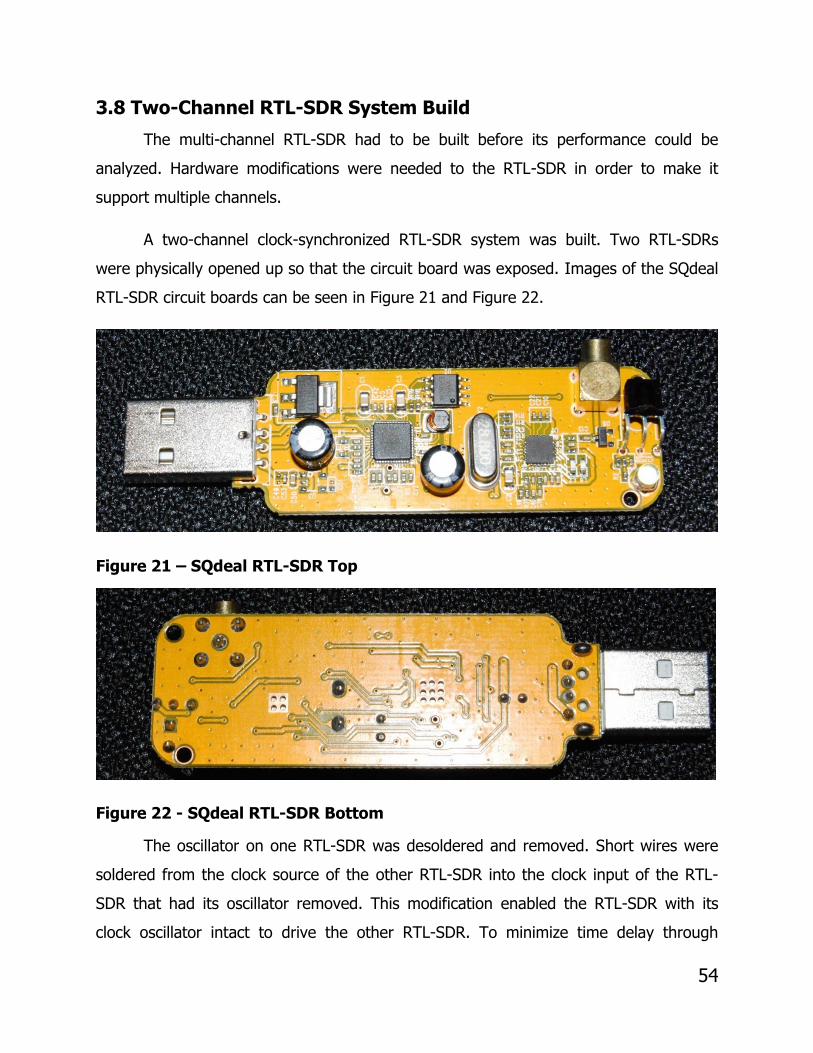
54
3.8 Two-Channel RTL-SDR System Build
The multi-channel RTL-SDR had to be built before its performance could be
analyzed. Hardware modifications were needed to the RTL-SDR in order to make it
support multiple channels.
A two-channel clock-synchronized RTL-SDR system was built. Two RTL-SDRs
were physically opened up so that the circuit board was exposed. Images of the SQdeal
RTL-SDR circuit boards can be seen in Figure 21 and Figure 22.
Figure 21 – SQdeal RTL-SDR Top
Figure 22 - SQdeal RTL-SDR Bottom
The oscillator on one RTL-SDR was desoldered and removed. Short wires were
soldered from the clock source of the other RTL-SDR into the clock input of the RTL-
SDR that had its oscillator removed. This modification enabled the RTL-SDR with its
clock oscillator intact to drive the other RTL-SDR. To minimize time delay through

55
wiring, the wires used were the shortest wires available that still allowed for the
physical connection of the RTL-SDRs to separate USB ports. Figure 23 and Figure 24
each show one side of the two-channel RTL-SDR. In Figure 24, the crystal oscillator is
the large silver component with the marking that reads 28.800. Figure 25 shows the
two-channel RTL-SDR system with the blue casing put back on after the modifications
were made.
Figure 23 – Modified Two-Channel RTL-SDR. Upper RTL-SDR with Oscillator Removed. Connection Soldered to Oscillator on Lower RTL-SDR.

56
Figure 24 – Modified Two-Channel RTL-SDR. Upper RTL-SDR Oscillator
Soldered to Lower RTL-SDR.
Figure 25 – Modified Two-Channel RTL-SDR with Casing
To confirm that the modification worked, each RTL-SDR in the two-channel
system was connected to its own USB port on the computer. Next, the rtl_test

57
command from the RTL-SDR software package was run to ensure that both RTL-SDR
devices were detected on the computer. Then, GNU Radio was used to receive data
along with a signal generator that was used to ensure that reception was possible from
both devices. These tests verified that the two-channel RTL-SDR system was functional
and that both devices were able to receive signals from the signal generator properly.
3.9 Two-Channel RTL-SDR System Phase Testing
After the two-channel RTL-SDR system was built, the next step was to determine
the phase offset between the two receivers.
3.9.1 Rise Time Delay Methods
The phase delay of the two-channel RTL-SDR system was measured by sending
a CW tone from the Agilent N5181A signal generator to each of the RTL-SDRs through
a splitter. A diagram of the hardware setup can be seen in Figure 26. Both RTL-SDRs in
the two-channel setup were connected directly to USB ports on the Linux computer.
First, the signal generator was initially off. Second, both RTL-SDRs were configured to
collect data at a center frequency of 895 MHz and a sample rate of 2 MHz for five
seconds, simultaneously. Third, after both RTL-SDRs began collecting data, the signal
generator was manually turned on and began outputting a -10-dBm signal at 895 MHz.
The -10 dBm amplitude signal was chosen because it is well above the noise floor and
below the saturation region. Fourth, the signal generator was then turned off about two
seconds after being turned on. The two RTL-SDRs were configured identically to acquire
data as soon as they were turned on via the modified rtl_sdr command on the
computer. As soon as the first sample was received on the computer, the modified
program would print out the current Unix timestamp in seconds and nanoseconds since
1970. The only difference between the original rtl_sdr program and the modified
program is that the modified one was recompiled to print the timestamp when the first
USB packet was processed by the rtl_sdr program on the computer. The collected data
points can be used to determine how much lag there was between the startup of both
RTL-SDRs.

58
Figure 26- Two-Channel Phase Testing Hardware Setup
The phase delay can be calculated by finding the time delay of a known input
into the receivers. Since samples occur at a fixed rate, the time delay is the number of
samples in the delay between the leading edge samples in the collected files, divided by
the sample rate. This calculation is shown in Equation 3, where t is the time delay,
sample diff is the difference in sample count between the start of the input signal in the
data files, and sample rate is the rate at which the receiver accumulates data samples.
In the case of this test setup, the sample rate is 2 MHz.
𝒕 = (𝒔𝒂𝒎𝒑𝒍𝒆 𝒅𝒊𝒇𝒇)/(𝒔𝒂𝒎𝒑𝒍𝒆 𝒓𝒂𝒕𝒆)
Equation 3 - Time Delay Calculation
A plot of the two-channel magnitude data collected without any phase correction
can be seen in Figure 27. In addition, since there were five seconds of sample data
collected and the time delay was only 1.529 milliseconds, an enlarged version of Figure
27 is shown in Figure 28.

59
Figure 27 - Time Lag of Two-Channel RTL-SDR System without Time Correction
Figure 28 – Enlarged Portion of Figure 27 Showing when RTL-SDR 2 Comes
on with Respect to RTL-SDR 1

60
Since the timestamp printed by the rtl_sdr program contained both the seconds
and nanoseconds since the year 1970, the two timestamps could be compared to see
their time difference. Next, with both timestamps from sample collection known, these
data could be fed into MATLAB to adjust for the phase lag. A plot of the two-channel
magnitude data shown in Figure 28 and Figure 29, with the correction for when the first
sample was received can be seen in Figure 29.
Figure 29 - Phase Lag of Two-Channel RTL-SDR System w/ Phase Correction
for First Sample Reception
3.9.2 Rise Time Delay Results
When the known signal was injected, it was possible to check which sample was
the first sample to record the input signal by checking which sample first had its
magnitude be greater than a noise threshold. The magnitude values recorded directly
correspond to the output of the ADC on the RTL-SDR.
After the Unix timestamp program was implemented and time correction was
performed, the time delay between starting samples was reduced from 1.529
milliseconds to 47.83 microseconds. After five tests with the sample being corrected, it
was determined that the time delay in the samples varied. Table 11 shows the time
delay data collected with and without the Unix timestamp correction.

61
Table 11 – Two-Channel RTL-SDR System Time Delays
Test Number Time Delay Time Delay (Corrected)
1 1.529 ms 47.83 usec
2 1.503 ms 30.19 usec
3 0.148 ms 41.28 usec
4 1.530 ms 80.19 usec
5 0.157 ms 4.26 usec
This variation is most likely caused by the USB interface. USB is a packet-based
protocol in which data are streamed to the computer from the RTL-SDR. Samples are
sent in the order they are collected, however data about when they were collected on
the RTL-SDRs are not available. There is also overhead on the Linux systems itself. The
way that the program interfaces with USB is event driven. This method of event
notification means that Linux will alert the program when there is USB data to read.
The time that it requires to do this notification depends on variables such as system
load. Although there is the Linux and USB overhead, the timestamp correction
significantly reduced the delay between channels.
3.9.3 Reception Stability Methods
Although the RTL-SDR was configured to receive at 895 MHz and the signal
generator was configured to output an 895 MHz signal, there was a low frequency wave
caused by the differences between the oscillators in the signal generator and the multi-
channel RTL-SDR. To compensate for this difference, the signal generator was instead
configured to output a known 895.05 MHz wave. This offset gave the RTL-SDR a 50
kHz wave that could be processed and used to determine the phase stability of the two
and three-channel RTL-SDR.

62
Figure 30- Two-Channel Reception Stability Setup with Signal Generator at
895.05 MHz
The low frequency wave caused by the oscillator difference, along with any high
frequency noise was filtered using a 6th order Butterworth band-pass filter with a pass-
band of 47 kHz to 56 kHz.
Figure 31 - 50 kHz Wave Received by the Two-Channel RTL-SDR System
Filtered by a Band-Pass Filter

63
After receiving and filtering the 50 kHz wave, the phases of the two channels of
the RTL-SDR system were compared. First, the filtered data were interpolated by a
factor of 10 using MATLAB’s interp function. Second, the peaks of each of the recorded
sine waves were found using the findpeaks command in MATLAB. Third, the difference
between the index corresponding to the first peak in the data from one channel and the
index corresponding to the first peak in the data from the second channel was
computed. Fourth, all of the indices of the second channel’s peaks were offset by this
difference. This offset essentially overlapped the 50 kHz wave present in both data sets
from the two-channels. Fifth, a difference between each peak index in the data from
the first channel and each peak index from the data from offset second channel was
taken. This time difference provided the phase results and gave a picture of how stable
the wave was reported in each RTL-SDR present in the two-channel system.
To ensure that the interpolation was helping to align the signal in time, the data
collected from the interpolated wave were compared against the data from the wave
that was not interpolated. It was suspected that interpolation would help because
interpolation effectively increases the sample rate in post-processing. This function was
implemented in MATLAB by using a low-pass filter and predicting the points that will fall
in between two points in a data set.
3.9.4 Reception Stability Results
The mean difference in time, along with the standard deviation between the
peaks in the data from the first channel and the peaks in the offset data from the
second channel, can be seen in Table 12. The test was repeated six times under the
same conditions.

64
Table 12 - Time Difference over 50 ms of Two-Channel Multi-RTL System
with a Signal Generator Operating at 895.05 MHz
Test Number Mean Time Difference Standard Deviation Time Difference
1 270.27 ns 320.08 ns
2 -222.78 ns 309.78 ns
3 79.579 ns 319.57 ns
4 92.151 ns 274.55 ns
5 -298.18 ns 292.09 ns
6 173.32 ns 284.10 ns
The interpolated data from the first three tests were compared against the data
from the signals that were not interpolated. A comparison of the interpolated data
versus the data without interpolation can be seen in Table 13. A histogram of the time
error from the interpolated data of Test 2 can be seen in Figure 32. On average, the
interpolated data had a lower standard deviation than the data that was not
interpolation by around 60 ns. This reduction was significant when compared to the full
standard deviation of around 380 ns.
Table 13 - Comparison of Interpolated Data Vs. Data with No Interpolation
Interpolated Data No Interpolation
Test # Mean(ns) Std. Dev(ns) Mean(ns) Std. Dev(ns)
1 270 320 317 381
2 -222 309 -226 378
3 79.5 319 -119 383

65
Figure 32 - Histogram of Test 2 of the Time Error for the Two-Channel RTL-
SDR System with Signal Generator at 895.05 MHz
To convert the results from samples into seconds, the samples had to be divided
by the sample rate to obtain the time difference in seconds. The time difference
calculation is shown in Equation 3. In order to determine phase from the time
difference in seconds, the time difference was multiplied by the frequency and then 360
to convert to degrees as shown in Equation 4. The results can be seen

66
Table 14. The frequency used for the phase calculation was the expected
frequency of 50 kHz which is found by using the difference of the signal generator
output frequency and the RTL-SDR reception frequency.
𝒑 = 𝒕 ∗ 𝒇 ∗ 𝟑𝟔𝟎
Equation 4 – Phase Difference Calculation

67
Table 14 - Phase Difference over 50 ms of Two-Channel Multi-RTL System
with a Signal Generator Operating at 895.05 MHz(f=50kHz)
Test # Mean of Phase Difference Standard Deviation of Phase Difference
1 4.86 degrees 5.76 degrees
2 -4.01 degrees 5.57 degrees
3 1.43 degrees 5.75 degrees
4 1.66 degrees 4.94 degrees
5 -5.37 degrees 5.25 degrees
6 3.11 degrees 5.11 degrees
3.9.5 Increased Frequency of Injected Signal Methods
In the original test, the frequency of the signal produced by the signal generator
that was fed into the two-channel RTL-SDR was 895.05 MHz. For this test, the
frequency was increased to 895.10 MHz with all other test conditions held constant. The
hardware setup for this test can be seen in Figure 33. The reason that this test was
conducted was because due to the offset of the oscillator in the signal generator vs the
oscillator in the RTL-SDR, a low noise wave of around 10 kHz was present in the data
collected by the RTL-SDR. Increasing the frequency of the injected signal to 895.10
MHz would allow for a higher frequency signal that was further away in frequency from
the predicted noise. The test was repeated three times under the same conditions.

68
Figure 33 - Two-Channel Reception Stability Setup with Signal Generator at
895.10 MHz
3.9.6 Increased Frequency of Injected Signal Results
The results of the increased frequency from the signal generator into the two-
channel RTL-SDR had worse phase results than the previous test at 895.05 MHz. These
results can be seen in Table 15 and Table 16 below.
Table 15 - Time Difference over 50 ms of Two-Channel Multi-RTL System
with a Signal Generator Operating at 895.10 MHz
Test # Mean of Time Difference Standard Deviation of Time Difference
1 -381.03 ns 275.30 ns
2 375.71 ns 364.80 ns
3 -179.89 ns 475.43 ns
Table 16 - Phase Difference over 50 ms of Two-Channel RTL-SDR System with a Signal Generator Operating at 895.10 MHz (f = 100 kHz)
Test # Mean of Phase Difference Standard Deviation of Phase Difference
1 13.75 degrees 9.91 degrees
2 13.53 degrees 13.13 degrees
3 6.48 degrees 17.12 degrees

69
3.10 Three-Channel RTL-SDR Build
After creating a two-channel RTL-SDR, a three-channel clock-synchronized RTL-
SDR system was created. Using the results from the clock stability test, the NooElec
NESDR Mini 2+ was chosen to drive two SQdeal Mini USB RTL-SDRs. Equal length wire
was used between the NooElec and each of the SQdeal receivers. The way that the
three-channel RTL-SDR was setup was comparable to the two-channel with the
difference that instead of one RTL-SDR clock coming off of the driving RTL-SDR, two
RTL-SDR clock lines were coming off one separate RTL-SDR. The NooElec RTL-SDR
looks different than the previous SQdeal RTL-SDR. Pictures of the NooElec RTL-SDR
opened up can be seen in Figure 34 and Figure 35.
Figure 34 - NooElec RTL-SDR Top
Figure 35 - NooElec RTL-SDR Bottom

70
The NooElec has a different oscillator, so the solder point going to the oscillator
inputs of the SQdeal RTL-SDRs is different than when using the SQdeal RTL-SDR as a
clock driver. Regardless, all of the three RTL-SDRs in the three-channel setup (NooElec
and two SQdeal models) were configured to collect data. The reason that the SQdeal
RTL-SDRs were chosen to be included in the three-channel SDR was because the way
to interface with them as a clock slave was known. Figure 36, Figure 37, and Figure 38
show different views of portions of the three-channel RTL-SDR system.
Figure 36 - NooElec RTL-SDR Top View Driving the Three-Channel System

71
Figure 37 - NooElec RTL-SDR Bottom View Driving the Three-Channel System

72
Figure 38 – Three-Channel RTL-SDR System with Casing
3.11 Three-Channel RTL-SDR Reception Stability
3.11.1 Reception Stability Methods
The process for the two-channel reception stability phase test was repeated
again three times for the three-channel RTL-SDR test. The hardware setup for the
three-channel test can be seen in Figure 39. The differences between the three-channel
test setup and the two-channel test setup are listed below:
1. Three SMA splitters were used to evenly distribute the signal from the signal
generator into the channels of the three-channel RTL-SDR.
2. Due to the number of USB ports present on the computer, a USB hub was used
to connect all three RTL-SDRs to one USB port on the computer.

73
Figure 39 - Three-Channel RTL-SDR Reception Stability Hardware Setup
The increased frequency of the signal generator from the two-channel test showed
that the phase difference of the two-channel RTL-SDR was worse when the frequency
of the signal generator was 895.10 MHz compared to 895.05 MHz. For this reason, the
signal generator was configured to output at 895.05 MHz. The three RTL-SDRs were
configured to collect 10 million samples (5 seconds of data) at a center frequency of
895.00 MHz, a sampling rate of 2 MHz, and a gain of 1.
In a very similar process as the two-channel RTL-SDR system, the three-channel
RTL-SDR system was started while the signal generator was initially off. After the RTL-
SDRs were verified to collect data, the signal generator outputted a -10 dBm amplitude
signal. Before the RTL-SDRs had each collected 10 million samples, the signal generator
was turned off.
Each test produced three data files, each data file held 10 million samples. These
data files were loaded into MATLAB for processing. First, each file was inspected to see
at what point in the file the data first started receiving the signal generator’s signal. The

74
data from each of the files was then reduced to the points in time from when the last
file to see the signal first saw data to 50 milliseconds later. The data were then filtered
using a band-pass filter with a pass-band of 47 kHz to 56 kHz with an order of 6. This
filter was a Butterworth filter. Next, the data were interpolated by a factor of 10 using
the interp command in MATLAB to make it easier to find the peaks of the signal in the
data. Next, the peaks of the wave were found using the findpeaks command in
MATLAB. The peaks were then overlapped by finding the lag between them. The
difference between the location of the peak in the first data file vs. the second data file
was added to the difference between the location of the peak in the first data file vs.
the second data file. This test would yield on average how stable the injected signal
was received in each of the three channels.
3.11.2 Reception Stability Results
The results of the three-channel test, shown in Table 17, Table 18, Table 19, and
Table 20, were generally higher by around a degree than the two-channel system. The
phase difference and time error for this test can be seen in Figure 40 and Figure 41,
respectively.
Table 17 – Mean Time Difference of Signal Detected by Three-Channel RTL-SDR System
Test # Ch. 1 vs. Ch. 2 Ch. 1 vs. Ch. 3 Ch. 2 vs Ch. 3
1 -336 ns -77.2 ns 258 ns
2 -613 ns -361 ns 253 ns
3 617 ns 619 ns 2.19 ns
Table 18 – Standard Deviation Time Difference of Signal Detected by Three-
Channel RTL-SDR System
Test # Ch. 1 vs. Ch. 2 Ch. 1 vs. Ch. 3 Ch. 2 vs Ch. 3
1 350 ns 369 ns 374 ns
2 319 ns 331 ns 349 ns
3 341 ns 376 ns 344 ns

75
Table 19 - Mean Phase Difference of Signal Detected by Three-Channel RTL-
SDR System
Test # Ch. 1 vs. Ch. 2 Ch. 1 vs. Ch. 3 Ch. 2 vs Ch. 3
1 -6.05 degrees -1.39 degrees 4.64 degrees
2 -11.1 degrees -6.50 degrees 4.55 degrees
3 11.1 degrees 11.1 degrees .039 degrees
Table 20 - Standard Deviation of Phase Difference of Signal Detected by
Three-Channel RTL-SDR System
Test # Ch. 1 vs. Ch. 2 Ch. 1 vs. Ch. 3 Ch. 2 vs Ch. 3
1 6.30 degrees 6.64 degrees 6.73 degrees
2 5.74 degrees 5.96 degrees 6.28 degrees
3 6.14 degrees 6.77 degrees 6.19 degrees
Figure 40 - 50 kHz Wave Received by the Three-Channel RTL-SDR System Filtered by a Band-Pass Filter

76
Figure 41 - Histogram of Peak Location Time Error in Three-Channel System Receiving an 895.05 MHz wave
Overall, the three-channel RTL-SDR could successfully receive the signal
generated by the signal generated and was around a degree more out of phase than
the two-channel system.

77
4.0 Discussion
All performance testing of standalone SDRs showed that RTL-SDRs do not match
the performance of the USRP. The received sample ratio testing revealed that RTL-
SDRs regularly drop samples above a sample rate of 2.85 MHz, while the USRP never
dropped samples up through 3.2 MHz, the maximum sample rate in the test. This result
indicates that RTL-SDRs would not be able to replace a USRP in a situation where
sampling above 2.85 MHz is necessary.
The noise floor performance testing indicated that the noise floor of RTL-SDRs at
approximately -60 dBm is much higher than the noise floor of the USRP at
approximately -85 dBm. This result indicates that the input power of a signal would
have to be higher to be discernible in an RTL-SDR than in a USRP. This noise floor
information also implies that the SNR of the RTL-SDRs is significantly lower than that of
the USRP.
The noise figure performance testing did not provide any conclusive noise figure
values for RTL-SDRs or the USRP, though the testing did show that the noise figure
performance of the RTL-SDRs is worse than that of the USRP. Since the recorded noise
figure values through two separate testing methods produced drastically different
results from one another, as well as different results from the expected values, no
further conclusions can be drawn from this information.
The frequency coverage performance testing indicated that the RTL-SDR can
reliably receive signals except at the ends of its frequency range of 24-1766 MHz,
whereas the USRP can reliably receive signals throughout this frequency range. This
result indicates that an RTL-SDR would not be able to replace a USRP where reception
of a signal at the ends of this frequency range is required. The frequency coverage
performance testing did show, however, that both the RTL-SDRs and the USRP did
receive a wideband signal, notably a 50-kHz noise signal meant to simulate ADS-B.

78
During the standalone performance testing of the RTL-SDRs, there were certain
issues that arose. The first issue was in the ADC unit calibration of the SDRs. For most
of the standalone performance testing of RTL-SDRs and the USRP, the data were
collected through GNU Radio. It was expected that the data recorded from GNU Radio
would be in terms of ADC counts, providing a range of values from 0 through 255 from
the RTL-SDR 8-bit ADCs and from 0 through 16383 from the USRP 14-bit ADC. The
data that were collected, however, was in terms of very small floating-point values with
much finer precision between one another than the separation between ADC counts in
bits.
Initially, there were concerns about whether the data were being read in the
correct format through MATLAB, but direct viewing of the bits within the data files
through a hex editor verified the collected results. It was eventually found possible to
find volt conversion factors from these floating-point values; therefore, it was possible
to convert the magnitude data from GNU Radio from these floating-point values to
calibrated units such as volts or dBm. It seems as though GNU Radio scales the raw
ADC count data from the SDRs by a linear factor to produce floating-point values.
Although it is not clear why this scaling occurs, it did not tangibly affect any test results.
Another issue that arose was in the noise figure testing results. As mentioned
previously, the results for noise figure cannot be considered credible, since the results
from different tests are so different from one another and so different from the
expected results. Although it is not known why the noise figure values collected from
these tests are inconsistent with expectations, there are certain tasks that can be
completed in the future to more conclusively determine the noise figures of SDRs. For
example, certain methods for measuring noise figure require knowledge of a parameter
of the input signal generator called the excess noise ratio (Agilent Technologies, 2010).
None of the equipment used for this project had a documented excess noise ratio
value, which made any noise figure measurement methods requiring this metric
impossible. In addition, the hardware setup did not include a low-noise amplifier. This
may have caused the noise floors of the SDRs in the calibration curves to be much

79
higher than expected, which would affect calculation of noise figure results. In the
future, performing the noise figure testing using equipment with a known excess noise
ratio and including a low noise amplifier would provide a better potential method of
measuring noise figure.
Given that air surveillance is a potential use case for RTL-SDRs, it is important to
consider its capabilities for this purpose. The radar range equation can be used to show
an example of how effectively both RTL-SDRs and a USRP could be used to detect ADS-
B signals from aircraft. The radar range equation can be solved for SNR of a signal at
the receiver. Assuming an ideal environment with unity transmitter and receiver gain,
no consideration for radar cross section since no radar reflection occurs, and a one-way
path, solving Equation 1 for SNR in dB provides Equation 5 below.
𝑺𝑵𝑹 = 𝟏𝟎 ∗ 𝐥𝐨𝐠𝟏𝟎 (𝑷𝑻 ∗ 𝒄𝟐
(𝟒𝝅)𝟐 ∗ 𝒇𝟎𝟐 ∗ 𝑹𝟐 ∗ 𝒌𝑻𝟎 ∗ 𝑩 ∗ 𝑭𝒏
) 𝒅𝑩
Equation 5 – Radar Range Equation (Richards, Scheer, & Holm, 2010)
For this example, f0 is 1090x106 Hz for the ADS-B signal carrier frequency, B is
2x10⁶ Hz for the bandwidth at the receiver, and c and kT0 are known constants. PT is
either 175 watts or 12.5 watts for the average power from a high-strength or low-
strength ADS-B transmitter given in Table 3. Since the noise figure results from testing
were inconclusive, the values for Fn used for this example are the documented values of
8 dB for the USRP, 13.6 dB for the RTL-SDR minimum, and 17 dB for the RTL-SDR
maximum. R is the range between the ADS-B transmitter and the SDR receiver in
meters, which is used as the independent variable for this example. Substituting all
values as described in the example above into Equation 5 gives results as shown below
in Figure 42 and Figure 43 for a high-strength and low-strength ADS-B transmitter,
respectively.

80
Figure 42 - Receiver SNR as a Function of Radar Range with High-Strength
ADS-B Transmitter
Figure 43 - Receiver SNR as a Function of Radar Range with Low-Strength
ADS-B Transmitter
In Figure 42 and Figure 43, the blue curves represent the USRP performance,
the orange curves represent the RTL-SDR best-case performance, and the yellow
curves represent the RTL-SDR worst-case performance. These curves show the SNR for

81
each SDR as a function of the range between an ADS-B transmitter and the given SDR
receiver. As can be seen in each figure, the USRP consistently has a higher SNR than
the RTL-SDR at each value for range, given its lower noise figure. In addition, the USRP
maintains a positive SNR up through a higher range than the RTL-SDR. These results
indicate that a USRP in either of these example situations can better receive ADS-B
signals than an RTL-SDR at a higher range. In the high-strength transmitter scenario,
the USRP maintains a positive SNR until a range of 1289 km, while the RTL-SDR
maintains a positive SNR until a range between 457 km and 677 km. In the low-
strength transmitter scenario, the USRP maintains a positive SNR until a range of 345
km, while the RTL-SDR maintains a positive SNR until a range between 122 km and 181
km. It is important to note that an RTL-SDR is still able to receive an ADS-B signal with
a high SNR up through a certain range, meaning that an RTL-SDR would be sufficient
for ADS-B reception in applications within a certain proximity.
The two-channel RTL-SDR system and the three-channel RTL-SDR system were
successfully built with a synchronized system clock oscillator, though certain issues
arose during development of these systems. An issue that occurred between all
channels in each multi-channel system was synchronization of sample collection. The
rise time testing showed that each RTL-SDR device within a multi-channel system would
begin data collection at different times, meaning that further processing would need to
be done on the data to properly align samples collected by each device. This method
could either be done via signal processing in real time to synchronize the devices after a
calibration period, or it could be done in post-processing by analyzing similar features at
different sample offsets within the collected data.
An issue faced with the three-channel RTL-SDR system involved the different
brands of RTL-SDRs used in the system. In the two-channel system, only SQdeal
devices were used, and available documentation indicated exactly where on the boards
of SQdeal RTL-SDRs soldering connections were needed. The three-channel system
used a NooElec RTL-SDR as a driver for two SQdeal RTL-SDRs. The clock oscillator and
the board layout of NooElec RTL-SDRs are different than those for SQdeal RTL-SDRs, so

82
it was initially difficult to determine where soldering connections needed to be made for
the three-channel system. This issue was resolved by using an oscilloscope to find the
pins of the clock oscillator from the NooElec device, and then soldering necessary
connections to these locations.
The phase testing of the two-channel and three-channel RTL-SDR systems
showed that, on average, the two-channel system was more in phase than the three-
channel system. It might be possible to decrease the standard deviation of the phase
difference within these systems through more advanced digital signal processing on the
input signal. It might also be possible to lower the standard deviation of the phase
difference by increasing the sample rate of the RTL-SDRs within the systems from the 2
MHz used during the phase tests. Doing such work might show improved stability of the
phase difference between devices in a multi-channel RTL-SDR system, thus increasing
the capabilities of such a system.
Geolocation might be possible using a multi-channel RTL-SDR system. Since
geolocation requires at least three channels, it would not be possible to use a two-
channel RTL-SDR system for this purpose, but a three-channel system or larger may be
sufficient for this purpose. It is difficult to know how low a phase tolerance is necessary
for geolocation, given that there are many possible methods of geolocation and phase
noise can have a variety of effects on such an application. Future work could be done to
test a multi-channel RTL-SDR system for geolocation of a known signal at a known
location in order to check its accuracy for this purpose. If such testing determines that
geolocation is not feasible with such a system, further signal processing could be
implemented in an effort to minimize phase noise and hopefully produce more accurate
results. Simulation can be done with these phase tolerances to see how feasible
geolocation is with the three-channel RTL-SDR.
The two-channel or three-channel RTL-SDRs can be tested to receive the same
signal and see if they can reduce the noise of the signal. The multi-channel RTL-SDRs

83
can be tested to see if they can receive a signal in which the bandwidth of it is larger
than the reception bandwidth of a single RTL-SDR.
84
5.0 Conclusion
One goal of this project was to analyze the performance characteristics of
hobbyist-grade RTL-SDRs and compare this performance to a well-known commercial-
grade radio, the USRP. Testing of the SDRs at various sample rates indicated that the
RTL-SDRs maintain a perfect received sample ratio up through 2.85 MHz but show very
poor performance above this sample rate, whereas the USRP has a perfect received
sample ratio throughout a sample rate range of 2.0 MHz to 3.2 MHz. The noise floors of
the RTL-SDRs at around -60 dBm were found to be much higher than the USRP noise
floor of about -85 dBm. The frequency coverage testing of the SDRs indicated that both
SDRs could properly receive a 50-kHz bandlimited white signal. The RTL-SDRs were
only reliably able to receive signals within a center frequency range of 50 MHz to 1600
MHz, while the USRP was able to receive signals through the entire tested center
frequency range of 24 MHz to 1766 MHz. Testing to determine the noise figure was
inconclusive in terms of absolute results, but showed that the noise figure of the RTL-
SDRs is higher than the noise figure of the USRP. These results indicate that the USRP
consistently performs better than RTL-SDRs, but that an RTL-SDR may be acceptable
for signal reception depending on situational requirements.
Another goal of this project was to build and test a multi-channel RTL-SDR
system. The oscillators of the RTL-SDRs were tested for clock jitter. The NooElec RTL-
SDR was chosen to have its oscillator drive the other two RTL-SDRs in the three-
channel system. Two-channel and three-channel RTL-SDR systems were built by using
the clock from one of the RTL-SDRs in each system to drive the other RTL-SDRs in the
system. These multi-channel systems were verified to be functional, and all RTL-SDR
channels were able to connect to a computer and collect data. The phase offset
between RTL-SDRs in each multi-channel system was tested by injecting a known 50-
kHz CW signal from a signal generator through splitters to each channel within each
system. Digital filtering and interpolation were performed in post-processing to make
the received signal clearer, and analysis was performed to determine the phase offset

85
of each received signal between RTL-SDRs within a multi-channel system. The RTL-
SDRs within the two-channel system were consistently within six degrees of one
another(around 300 ns at 50 kHz), and the RTL-SDRs within the three-channel system
were also consistently within six degrees of one another.
The two-channel and three-channel RTL-SDR systems given to Group 108 at the
end of the project were functional and their system clock oscillators were synchronized
via hardware. The remaining standalone RTL-SDR devices were also operational.
Further testing and signal processing can be done to determine the capabilities of a
standalone RTL-SDR to receive a signal over the air, such as an ADS-B signal from an
aircraft. Further testing and signal processing can also be done to determine whether or
not a multi-channel RTL-SDR system can feasibly be used for geolocation of a signal
source.

86
Works Cited
About RTL-SDR. (2013). Retrieved August 15, 2016, from RTL-SDR.COM:
http://www.rtl-sdr.com/about-rtl-sdr/
Agilent Technologies. (2010, August 5). Agilent Fundamentals of RF and Microwave
Noise Figure Measurements. Retrieved from Agilent Technologies:
http://cp.literature.agilent.com/litweb/pdf/5952-8255E.pdf
Ettus Research. (2016). USRP X310. Retrieved from Ettus Research:
https://www.ettus.com/product/details/X310-KIT
Federal Aviation Administration. (2016, July 27). Automatic Dependent Surveillance -
Broadcast. Retrieved from Federal Aviation Administration:
http://www.faa.gov/nextgen/programs/adsb/
International Civil Aviation Organization. (2007, February 26). Aeronautical
Telecommunications. Retrieved September 26, 2016, from ADS-B Technologies:
http://www.ads-b.com/PDF/UAT%20SARP.pdf
Krysik, P. (2016, May). Multi-RTL. Retrieved from Piotr Krysik's Webpage:
https://ptrkrysik.github.io/
MIT Lincoln Laboratory. (2016). Technical Divisions. Retrieved from MIT Lincoln
Laboratory: http://www.ll.mit.edu/employment/division10.html#108
MIT Lincoln Laboratory. (n.d.). Air, Missile, & Maritime Defense Technology. Retrieved
from Lincoln Laboratory:
http://www.ll.mit.edu/mission/airmissle/airmissledefense.html
National Instruments. (2016, March 30). What is I/Q Data? Retrieved from National
Instruments: http://www.ni.com/tutorial/4805/en/

87
National Telecommunications & Information Administration. (2014, March 1). 960-1164
MHz. Retrieved October 7, 2016, from National Telecommunications &
Information Administration:
http://www.ntia.doc.gov/files/ntia/publications/compendium/0960.00-
1164.00_01MAR14.pdf
Pu, D., & Wyglinski, A. M. (2013). Nyquist Sampling Theorem. In Digital Communication
Systems Engineering with Software-Defined Radio (pp. 26-27, 98). Boston,
Massachusetts: Artech House.
Richards, M. A., Scheer, J. A., & Holm, W. A. (2010). Basic Principles. In Principles of
Modern Radar (pp. 59-66). Edison, NJ: SciTech Publishing.
Rosu, I. (n.d.). Understanding Noise Figure. Retrieved October 3, 2016, from YO3DAC -
VA3IUL: www.qsl.net/va3iul/Noise/Understanding%20Noise%20Figure.pdf
RTL-SDR Blog. (2015, March 31). Some E4000 RTL-SDR Noise Figure Measurements.
Retrieved October 3, 2016, from RTL_SDR.COM: http://www.rtl-sdr.com/some-
e4000-rtl-sdr-noise-figure-measurements/
SiTime Corporation. (2014). Clock Jitter Definitions and Measurements Methods.
Sunnyvale, California: SiTime Corporation.
Smyrna Air Center, Inc. (n.d.). ADS-B1. Retrieved from
http://www.smyrnaaircenter.com/wp-content/uploads/2012/08/ADS-B1.jpg
Stallings, W. (2014). Data and Computer Communications. 72.