Embed Size (px)
Citation preview

Analysis and Design of Software-Based
Optimal PID Controllers
Olof Garpinger
Department of Automatic Control

Present, Past, Future. The picture on the upper hand of the front covershows two parts of a longcase clock made by the Swedish woodcarverand artist Jöns Mårtensson. The parts have been slightly modified by thethesis author.
PhD ThesisISRN LUTFD2/TFRT--1105--SEISBN 978-91-7623-271-2 (print)ISBN 978-91-7623-272-9 (web)ISSN 0280–5316
Department of Automatic ControlLund UniversityBox 118SE-221 00 LUNDSweden
© 2015 by Olof Garpinger. All rights reserved.Printed in Sweden by Media-Tryck.Lund 2015

To Linda-Marie and Wilmer


Abstract
A large process industry can have somewhere between five hundred andfive thousand control loops, and PID controllers are used in 90–97% of thecases. It is well-known that only 20–30% of the controllers in the processindustry are tuned satisfactorily, but with the methods available today itis considered too time-consuming to optimize each single controller. Thisthesis presents tools for analysis and design of optimal PID controllers,and suggests when and how to use them efficiently. High performing low-level controllers are also likely to be beneficial for higher-level advancedprocess control, thus promoting the economy of whole factories.Controller design is often a trade-off between conflicting criteria, such
as load disturbance attenuation, robustness, and noise sensitivity. In thisthesis, a MATLAB®-based software tool is used to solve a constrainedoptimization problem, with respect to all three requirements. This givestuning of both the PID parameters and a low-pass filter time constant.A large batch of benchmark models, representative for the process in-
dustry, has been used throughout the whole thesis for controller analysis.This includes comparisons between PID controllers derived using eitheroptimization or tuning rules. Trade-off plots are also presented, which ex-plicitly show the relationships between performance, robustness and thePID parameters.A new procedure for software-based optimal PID design is suggested,
which leads to a set of PID, PI, and I controllers. The user can then selectthe best performing controller with an acceptable control signal activity. Itis shown that the resulting controllers are optimal or near optimal withrespect to the three above mentioned criteria. The same procedure canalso be used to analyze the benefit of the derivative part by comparingoptimal PI and PID controllers with the same level of noise sensitivity. Theefficiency of the procedure is demonstrated on an industrial friction stirwelding machine. For a more wide-spread use of the proposed procedure,it is shown that better modeling techniques are needed, and guidelinesfor such methods are also included.
5


Acknowledgments
First, I would like to thank all my colleagues at the Department of Auto-matic Control, Lund University, for giving me such a warm welcome backafter spending a few years in the industry. I am especially grateful toTore Hägglund and Karl-Johan Åström for asking me to come back andfor convincing me that it was a good idea. I have really enjoyed workingtogether with all of you again.I am very fortunate to have had Tore Hägglund as my supervisor.
My work is deeply influenced by his ambition to make research usefulin practice, and he has opened my eyes to the beauty of simplicity. Froma personal point of view, I truly believe that his wisdom has helped mebecome a better man.It is a rare luxury to have worked with someone as talented and full
of energy as Karl-Johan Åström. I want to thank you for all your adviceover the years, it has granted me a lot of insight into PID control.During my first years at the department, I shared (countless) offices
with Per-Ola Larsson. I am very thankful for the many discussions wehave had, and during which I think we converged to more or less thesame visions for the future of PID design.I would like to thank SKB for giving me the opportunity to work on
their friction stir welding machine. A special thanks to Lars Cederqvist,for helping me regain my self confidence and for introducing me to FSW.I am grateful to Anders Robertsson for introducing me to Lars. I amalso glad that I have had the chance to work with two brilliant controlengineers on the SKB project, namely Anton Cervin and Isak Nielsen.Several of my colleagues have helped me proofread my articles and
thesis. Therefore, I would like to thank: Tore Hägglund, Per-Ola Lars-son, Karl-Johan Åström, Lars Cederqvist, Anton Cervin, Kristian Soltesz,Martin Hast, and Anders Robertsson.I am very thankful for all the help Leif Andersson has provided during
the work on this thesis. His knowledge in LATEX is invaluable. I would also
7

like to thank the rest of our Research Engineers as well as our Adminis-trators for making the department run so smoothly. This includes our pre-vious employees: Eva Schildt, Britt-Marie Mårtensson, Agneta Tuszynski,Lizette Borgeram, and Rolf Braun.I would like to send my warmest appreciations to both my own par-
ents and my parents-in-law, for helping me and my wife finish our thesesthrough countless hours of babysitting. Finally, I would like to say that Iam the most fortunate man to have such a wonderful wife as Linda-Marie,and such lovely son as Wilmer. You mean the world to me.
8

Contents
1. Introduction 181.1 The closed-loop system . . . . . . . . . . . . . . . . . . . . 181.2 The PID controller . . . . . . . . . . . . . . . . . . . . . . . 191.3 Process industrial context . . . . . . . . . . . . . . . . . . . 22
2. Models and modeling for the process industry 262.1 Process models and process classification . . . . . . . . . . 262.2 Modeling methods . . . . . . . . . . . . . . . . . . . . . . . 272.3 Benchmark models for the process industry . . . . . . . . 28
3. Criteria and trade-offs for PID design 313.1 Performance . . . . . . . . . . . . . . . . . . . . . . . . . . 313.2 Robustness . . . . . . . . . . . . . . . . . . . . . . . . . . . 333.3 Noise sensitivity . . . . . . . . . . . . . . . . . . . . . . . . 333.4 Constrained optimization of PID controllers . . . . . . . . 35
4. PID design methods 364.1 Tuning rules . . . . . . . . . . . . . . . . . . . . . . . . . . 364.2 Optimization-based methods . . . . . . . . . . . . . . . . . 41
5. Friction stir welding 445.1 Background . . . . . . . . . . . . . . . . . . . . . . . . . . . 445.2 FSW of thick copper canisters for nuclear waste . . . . . . 455.3 PID design for an FSW process . . . . . . . . . . . . . . . 46
6. Thesis contributions 486.1 Thesis objectives . . . . . . . . . . . . . . . . . . . . . . . . 486.2 Contributions . . . . . . . . . . . . . . . . . . . . . . . . . . 486.3 Visions and future work . . . . . . . . . . . . . . . . . . . . 51
Bibliography 53
Paper I. Performance and robustness trade-offs in PIDcontrol 61
1 Introduction . . . . . . . . . . . . . . . . . . . . . . . . . . . 622 Controllers and design criteria . . . . . . . . . . . . . . . . 63
9

Contents
3 The trade-off plot . . . . . . . . . . . . . . . . . . . . . . . . 654 Tuning methods . . . . . . . . . . . . . . . . . . . . . . . . 695 Assessment of tuning methods . . . . . . . . . . . . . . . . 746 PID control . . . . . . . . . . . . . . . . . . . . . . . . . . . 777 Conclusions . . . . . . . . . . . . . . . . . . . . . . . . . . . 81References . . . . . . . . . . . . . . . . . . . . . . . . . . . . . . . 83
Paper II. A software tool for robust PID design 871 Introduction . . . . . . . . . . . . . . . . . . . . . . . . . . . 882 Design criterion . . . . . . . . . . . . . . . . . . . . . . . . 893 Algorithm overview . . . . . . . . . . . . . . . . . . . . . . 904 Algorithm details . . . . . . . . . . . . . . . . . . . . . . . . 925 Examples . . . . . . . . . . . . . . . . . . . . . . . . . . . . 986 Conclusions . . . . . . . . . . . . . . . . . . . . . . . . . . . 101References . . . . . . . . . . . . . . . . . . . . . . . . . . . . . . . 103
Paper III. Modeling for optimal PID design 1051 Introduction . . . . . . . . . . . . . . . . . . . . . . . . . . . 1062 Theory . . . . . . . . . . . . . . . . . . . . . . . . . . . . . . 1063 Comparison of the tuning methods . . . . . . . . . . . . . 1094 Model quality . . . . . . . . . . . . . . . . . . . . . . . . . . 1125 Results . . . . . . . . . . . . . . . . . . . . . . . . . . . . . . 1146 Conclusions . . . . . . . . . . . . . . . . . . . . . . . . . . . 117References . . . . . . . . . . . . . . . . . . . . . . . . . . . . . . . 118
Paper IV. Software-based optimal PID design withrobustness and noise sensitivity constraints 121
1 Introduction . . . . . . . . . . . . . . . . . . . . . . . . . . . 1222 Theoretical background . . . . . . . . . . . . . . . . . . . . 1243 Performance and noise sensitivity trade-off . . . . . . . . 1324 Controller optimality and robustness level selection . . . 1365 PID design procedure . . . . . . . . . . . . . . . . . . . . . 1396 Benefits of the derivative part . . . . . . . . . . . . . . . . 1427 Conclusions and discussion . . . . . . . . . . . . . . . . . . 1468 Acknowledgements . . . . . . . . . . . . . . . . . . . . . . . 150References . . . . . . . . . . . . . . . . . . . . . . . . . . . . . . . 150
Paper V. Cascade control of the friction stir weldingprocess to seal canisters for spent nuclear fuel 153
1 Introduction . . . . . . . . . . . . . . . . . . . . . . . . . . . 1542 Process description . . . . . . . . . . . . . . . . . . . . . . . 1553 Controlling the FSW process . . . . . . . . . . . . . . . . . 1614 Experimental setup . . . . . . . . . . . . . . . . . . . . . . 1675 Results and discussion . . . . . . . . . . . . . . . . . . . . 1716 Conclusions . . . . . . . . . . . . . . . . . . . . . . . . . . . 180References . . . . . . . . . . . . . . . . . . . . . . . . . . . . . . . 182
10

Contents
Supplement to Paper V 185S.1 Inner-loop control design . . . . . . . . . . . . . . . . . . . 185S.2 Outer-loop control design . . . . . . . . . . . . . . . . . . . 187S.3 Results on the FSW process . . . . . . . . . . . . . . . . . 190S.4 Conclusions . . . . . . . . . . . . . . . . . . . . . . . . . . . 191
11


Preface
Contents and contributions of the thesis
This thesis consists of six introductory chapters and five papers. Thissection describes the contents of the introductory chapters and the con-tributions of each paper.
Chapter 1 – Introduction
The closed-loop system used to formulate a constrained optimization prob-lem for PID controller design is defined in this chapter. The differentparts of the PID controller are also defined. Finally, the thesis is put intoa process industrial context. Notice that the theory presented in Sections1.1–1.2 is standard PID material, see e.g. [Åström and Hägglund, 2005].
Chapter 2 – Models and modeling for the process industry
Some commonly used process models and modeling techniques for theprocess industry are introduced here together with a simple measure forprocess classification. A large batch of process models representative forthe process industry is also presented and motivated.
Chapter 3 – Criteria and trade-offs for PID design
Several commonly used performance, robustness and noise sensitivity cri-teria are presented, and the specific choices made for this thesis aremotivated. The chapter is ended with the formulation of a constrainedoptimization problem for design of a PID controller with a low-pass mea-surement noise filter.
Chapter 4 – PID design methods
Several commonly used PID tuning rules are introduced and their popu-larity is explained. The second section of the chapter presents differentoptimization-based PID design methods.
13

Contents
Chapter 5 – Friction stir welding
The friction stir welding process is explained here together with a briefdescription of the specific control application to seal copper canisters fornuclear waste.
Chapter 6 – Thesis contributions
Thesis objectives, contributions and future visions for software-based op-timal PID design are presented in this chapter.
Paper I
Garpinger, O., T. Hägglund, and K. J. Åström (2014). “Performance androbustness trade-offs in PID control”. Journal of Process Control 24:5,pp. 568–577.
This paper introduces new trade-off plots for PID control that showexplicitly how performance, with respect to load disturbances, and robust-ness depend on the controller parameters. Plots are given for processeswith lag-dominated, balanced and delay-dominated dynamics, for both PIand PID control. Both input and output disturbances are considered forPI control, and for PID control noise filtering is briefly analyzed. Theplots are also used to show strengths and weaknesses of some common PItuning rules.O. Garpinger and K.J. Åström constructed the trade-off plots. The
development of the plots has been carried out by all three authors throughnumerous discussions. The idea to compare different tuning rules camefrom O. Garpinger. The parametrization of optimal controllers was derivedby K.J. Åström. K.J. Åström and O. Garpinger have written most of thepaper, with assistance from T. Hägglund.
Paper II
Garpinger, O. and T. Hägglund (2008). “A Software Tool for Robust PIDDesign”. In: 17th IFAC World Congress. Seoul, South Korea.
The MATLAB®-based software presented in this paper finds optimalPID controllers with respect to minimum integrated absolute error dur-ing a unit load disturbance on the process input and H∞ robustness con-straints on the sensitivity and complementary sensitivity functions. Theoptimization problem is solved using a simplex-based algorithm called theNelder-Mead method. The resulting controllers are shown to give goodcontrol for a large batch of process models that are representative for theprocess industry. The software can both provide very good controllers ina short amount of time and be useful for PID control analysis.
14

Contents
The MATLAB®-based software was written by O. Garpinger, inspiredby the previous work by P. Nordfeldt (see citation in the paper). T. Häg-glund contributed with support and experience from PID design. The pa-per was written by O. Garpinger with assistance from T. Hägglund.
Paper III
Garpinger, O. and T. Hägglund (2014). “Modeling for Optimal PID De-sign”. In: 19th IFAC World Congress. Cape Town, South Africa.
In this paper, three commonly used PI and PID tuning rules are com-pared to optimal controller design with respect to performance and robust-ness. First order time delayed model approximations, derived from stepresponse tests, are used. All four methods are shown to have weaknessesin terms of performance and robustness variation or the lack of a tuningparameter, especially for PID control. It is investigated what process in-formation is desirable for design based on constrained optimization. ForPI control it is enough to have information around a single phase angle,while for PID control the desirable information depends on the normal-ized time delay of the process. Given such improved models it is shownthat performance and robustness can be kept close to optimal.The comparison of different tuning methods was carried out by
O. Garpinger. The desired process information for optimal PI and PIDdesign was investigated by O. Garpinger. O. Garpinger also derived theimproved models that are shown to work well with the given optimalPID design. T. Hägglund contributed with support and experience fromPID design. The paper was written by O. Garpinger with assistance fromT. Hägglund.
Paper IV
Garpinger, O. and T. Hägglund (2015). “Software-Based Optimal PID De-sign with Robustness and Noise Sensitivity Constraints”. Submittedto Journal of Process Control.
This paper presents a new optimal PID design method that takes per-formance, robustness and control signal noise sensitivity into account tofind both the three PID parameters and a low-pass filter time constant.The tuning method uses a Matlab-based software tool and results in aset of optimal or near-optimal PID, PI and I controllers, which the usercan switch between to select the best controller giving a maximum al-lowed control signal activity. No noise modeling is needed in the finaldesign procedure. A large batch of process models representative for theprocess industry is used to compare optimal PI and PID controllers with
15

Contents
the same noise sensitivity and robustness measures. This shows whichprocesses have the most to benefit from derivative action.O. Garpinger has plotted the performance, robustness and noise sen-
sitivity trade-offs that illustrate the relationship between optimal PID, PIand I controllers. O. Garpinger has developed the proposed PID designprocedure with support from T. Hägglund. The method for showing thebenefit of the derivative part has also been developed by O. Garpinger.The paper was written by O. Garpinger with support from T. Hägglund.
Paper V
Cederqvist, L., O. Garpinger, T. Hägglund, and A. Robertsson (2012).“Cascade control of the friction stir welding process to seal canistersfor spent nuclear fuel”. Control Engineering Practice 20:1, pp. 35 –48.
The Swedish Nuclear Fuel and Waste Management Company plans tojoin at least 12,000 lids and bases to the extruded copper tubes containingSweden’s nuclear waste, using friction stir welding. To ensure high qual-ity welds without defects or tool fractures, it is important to control thewelding temperature. The process is exposed to both quick torque distur-bances and power losses due to changing thermal boundary conditions.A cascade controller with two PI controllers for control of power inputand temperature is proposed and applied to the custom-built machine.It is shown that the cascade controller manages very well to keep thetemperature within the specified process window of 790− 910○C.The PID design method used in this paper is older than the one pre-
sented in Paper IV. The paper has thus been extended with a supplementto show the advantages of the new method when applied to the FSW pro-cess.The experimental set-up and all welds have been carried out by L. Ced-
erqvist. The high-level controller objectives were specified by L. Ced-erqvist. O. Garpinger developed the cascade control structure with sup-port from L. Cederqvist. Process modeling, controller selection and de-sign was carried out by O. Garpinger. Control strategies during thestart-up and parking sequences were developed by L. Cederqvist andO. Garpinger. T. Hägglund and A. Robertsson have contributed with theirexperience through numerous discussions. The paper has mostly beenwritten by O. Garpinger with support from L. Cederqvist, T. Hägglundand A. Robertsson. The paper supplement is work by O. Garpinger.
Additional peer-reviewed publications
Below is a list of additional peer-reviewed publications by the thesis au-thor that were decided not to be included in the thesis.
16

Contents
Cederqvist, L., O. Garpinger, T. Hägglund, and A. Robertsson (2010).“Cascaded Control of Power Input and Welding Temperature DuringSealing of Spent Nuclear Fuel Canisters”. In: Proc. ASME DynamicSystems and Control Conference. Cambridge, Massachusetts.
Garpinger, O., T. Hägglund, and K. J. Åström (2012a). “Criteria andTrade-offs in PID Design”. In: IFAC Conference on Advances in PIDControl. Brescia, Italy.
Garpinger, O., T. Hägglund, and L. Cederqvist (2012b). “Software for PIDDesign: Benefits and Pitfalls”. In: IFAC Conference on Advances in PIDControl. Brescia, Italy.
Nielsen, I., O. Garpinger, and L. Cederqvist (2013). “Simulation basedEvaluation of a Nonlinear Model Predictive Controller for Friction StirWelding of Nuclear Waste Canisters”. In: 2013 European Control Con-ference. Zürich, Switzerland.
17

1
Introduction
1.1 The closed-loop system
The single-input single-output feedback loop in Fig. 1.1 will be usedthroughout this thesis both for analysis and to set up a constrained opti-mization problem for the design of proportional integral derivative (PID)controllers. The process, P(s), is manipulated by a controller, C(s), suchthat the controlled variable, z, is kept as close as possible to a set-point, r,in order to minimize the control error, e. The process is affected by a loaddisturbance, d, at the process input. The measurements of the controlledvariable, y, typically contain noise, n, and are fed through a low-pass filter,F(s), to keep the noise level of the control signal, u, low.The choice of letting the load disturbance act on the process input is
supported by e.g. [Shinskey, 1996, p 5], that claims that this is the usualcase in process industrial control. The case of having a process outputdisturbance is, however, briefly investigated in Paper I.Assuming regulatory control around a constant set-point, r = 0, the
ΣΣΣ
e u y
P(s)C(s)
−F(s)
d n
r z
Figure 1.1 A load disturbance, d, measurement noise, n, and set-point,r, act on the closed-loop system with process P(s), controller C(s) andmeasurement filter F(s).
18

1.2 The PID controller
closed-loop system can be described by three equations
Z(s) = P(s)1+ P(s)C(s)F(s)D(s) −
P(s)C(s)F(s)1+ P(s)C(s)F(s)N(s), (1.1)
Y(s) = P(s)1+ P(s)C(s)F(s)D(s) +
11+ P(s)C(s)F(s)N(s), (1.2)
U(s) = − P(s)C(s)F(s)1+ P(s)C(s)F(s)D(s) −
C(s)F(s)1+ P(s)C(s)F(s)N(s), (1.3)
with frequency-domain signals in capital letters. It is well-known that thefour transfer functions
S(s) = 11+ P(s)C(s)F(s) , (1.4)
T(s) = P(s)C(s)F(s)1+ P(s)C(s)F(s) , (1.5)
Sp(s) =P(s)
1+ P(s)C(s)F(s) , (1.6)
Sc(s) =C(s)F(s)
1+ P(s)C(s)F(s) , (1.7)
are sufficient to describe the closed-loop system in Fig. 1.1. S(s) is calledthe sensitivity function and T(s) the complementary sensitivity function.
1.2 The PID controller
The main objectives of this thesis are to suggest methods for both designand analysis of the PID controller. The three PID controller parts willbe described in this section, together with some possible PID controllerforms and measurement filters.
Proportional part
The proportional part (P-part) of the control signal is proportional to thecontrol error,
up(t) = K ep(t) + u0, ep(t) = br(t) − y(t), (1.8)
such that it reacts to present deviations from the set-point. The propor-tional gain, K , is the parameter normally associated with the P-part, butit is sometimes replaced by a parameter called the proportional band, see
19
Chapter 1. Introduction
e.g. [Shinskey, 1996]. A P controller alone cannot guarantee zero staticcontrol errors, since the control signal becomes zero for ep(t) = 0. The biasterm u0 is used to reduce this effect in controllers that lack an integralpart. The magnitude of the static error depends on K . The speed andnoise sensitivity of the closed-loop system will typically increase with anincreasing K at the same time as the robustness decreases. The P-part issensitive to noise since K is multiplied directly with the measurements,y(t), unless filtered first. Abrupt changes in the set-point can be smoothedout in the control signal by choosing a set-point weight 0 ≤ b < 1.
Integral part
The integral part (I-part) integrates past values of the control error,
ui(t) =K
Ti
t∫
0
e(τ )dτ = kit∫
0
e(τ )dτ , e(t) = r(t) − y(t), (1.9)
and will thus remove static control errors due to step load disturbancesand set-point changes. It introduces the integral time Ti, but also dependson the proportional gain K unless the fraction K/Ti is replaced by anindependent parameter, ki, called the integral gain. Reducing Ti normallyleads to a faster, although less robust, closed-loop system. The summationof past control errors makes the I-part insensitive to noise. A drawback ofthe I-part is that the controller implementation needs to handle so-calledintegrator wind-up, see e.g. [Åström and Hägglund, 2005, pp 76–77] formore information.
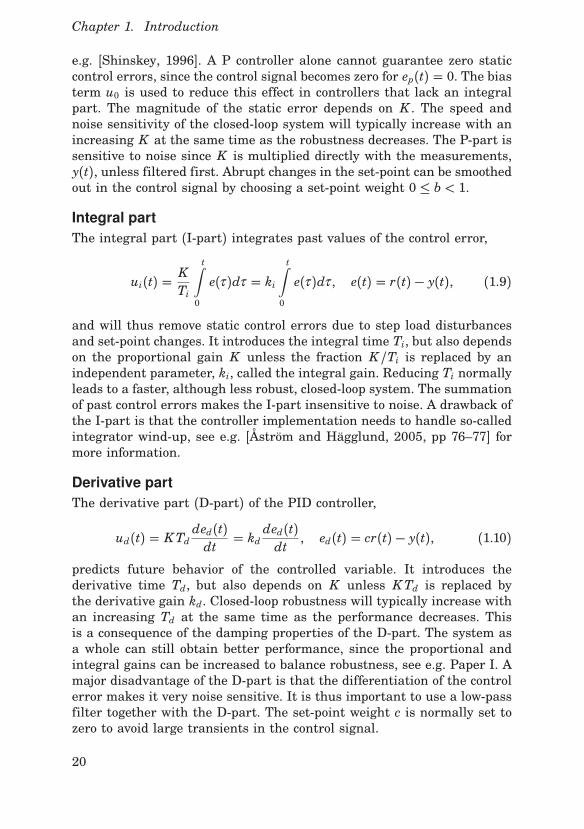
Derivative part
The derivative part (D-part) of the PID controller,
ud(t) = KTdded(t)dt
= kdded(t)dt
, ed(t) = cr(t) − y(t), (1.10)
predicts future behavior of the controlled variable. It introduces thederivative time Td, but also depends on K unless KTd is replaced bythe derivative gain kd. Closed-loop robustness will typically increase withan increasing Td at the same time as the performance decreases. Thisis a consequence of the damping properties of the D-part. The system asa whole can still obtain better performance, since the proportional andintegral gains can be increased to balance robustness, see e.g. Paper I. Amajor disadvantage of the D-part is that the differentiation of the controlerror makes it very noise sensitive. It is thus important to use a low-passfilter together with the D-part. The set-point weight c is normally set tozero to avoid large transients in the control signal.
20

1.2 The PID controller
Controller forms and measurement filters
There are several possible controller combinations that can be formedwith the three parts (1.8–1.10). The most common ones are P, I, PI, PDand PID control. I, PI and PID controllers will be considered in this thesis,since the majority of process industrial control applications benefit fromthe I-part.In the remaining part of this thesis all controllers will be described in
the frequency domain rather than in the time domain. The I controller,
CI(s) =ki
s, (1.11)
has only one parameter, ki. The PI controller is given by
CPI(s) = K(
1+ 1sTi
)
. (1.12)
For PID control there are two common forms: the parallel form,
CPID(s) = K(
1+ 1sTi
+ sTd)
, (1.13)
which just adds the D-part to the PI controller, and the series form,
C′PID(s) = K ′(1+ sT ′i )
(
1+ sT ′d)
sT ′i, (1.14)
which is convenient for design based on lead-lag compensation, see e.g.[Franklin et al., 2010]. For Ti ≥ 4Td, the parallel and series forms areequivalent. The parallel form is, however, more general since it can havecomplex zeros. [Hägglund and Åström, 2004] among others have previ-ously shown that this is often preferred. For this reason, the parallelform will be the main focus in this thesis, while the series form will onlybe used for comparison of different PID tuning methods.The low-pass filter is an important component of the PID controller
since the derivative part is very noise sensitive. There are several waysin which filtering can be implemented together with a PID controller, butit is common practice to use filters of order one either on the derivativepart alone,
CPIDF(s) = K(
1+ 1sTi
+ sTd
s(Td/N) + 1
)
, (1.15)
where N is usually a number between 5 and 10, or on the whole mea-surement signal,
F(s) = 1sT f + 1
. (1.16)
21

Chapter 1. Introduction
See e.g. [Isaksson and Graebe, 2002; Kristiansson and Lennartson, 2002;Šekara and Mataušek, 2009; Sadeghpour et al., 2012] for studies on thesefilter forms. An advantage with the measurement signal filter is that onecan design controllers for the combination P(s)F(s). This is the approachused in this thesis, but a second-order filter
FPID(s) =1
(sT f )2/2+ sT f + 1, (1.17)
has been used with PID control in order to guarantee amplitude roll-offfor high frequencies. FPID has two complex poles with relative dampingζ = 1/
√2, which is the smallest damping ratio for which there is no
amplitude increase caused by the filter. Some other studies [Larsson andHägglund, 2011; Romero Segovia et al., 2013; Micić and Mataušek, 2014]have also explored higher-order low-pass filters for PID control. A first-order filter
FPI(s) =1
sT f + 1, (1.18)
will be used here for PI control, also for the sake of high-frequency roll-off.The filter time constant T f is the only parameter that needs to be set inboth FPI and FPID . They would have been more general with two or moreparameters, but these forms were chosen to keep the amount of controllerparameters low. [Larsson and Hägglund, 2011] showed that the filters FPIand FPID are well suited for the closed-loop system in Fig. 1.1 and thatfilters of lower and higher order are not likely to give any performancebenefits for equivalent noise sensitivity when using white Gaussian noise.I control has natural roll-off, so FI(s) = 1.
1.3 Process industrial context
Even though the research presented in this thesis can be used on a widerange of processes (see e.g. Paper V), its main target is regulatory controlin the process industry. This section will, therefore, provide some back-ground on the process industrial control situation and show why the PIDcontroller fits so well into its framework.According to e.g. [Yamamoto and Hashimoto, 1991; Bialkowski, 1993;
Ender, 2001] the two main objectives of process control are to ensure asafe and stable process around the set-point and to minimize the vari-ation of the control error. This has to be accomplished in spite of con-stantly changing environment, equipment and raw materials [Forsman,2005]. Disturbances are typically not accessible before they have alreadyinfluenced the process under control.
22

1.3 Process industrial context
Large process industries typically have somewhere between five hun-dred and five thousand control loops [Yamamoto and Hashimoto, 1991;Bialkowski, 1993; Desborough and Miller, 2002]. The PID control algo-rithm is used to control almost all of these loops with relative numbersnormally as high as 90–97% [Yamamoto and Hashimoto, 1991; Bialkowski,1993; Ender, 1993; Desborough and Miller, 2002; Kano and Ogawa, 2010;Kuzu, 2012]. This predominance is largely a result of the following PIDcontroller properties:
1. Easy to understand [Desborough and Miller, 2002; Isaksson, 2012]
2. Works well for a majority of processes [Desborough and Miller, 2002;Isaksson, 2012]
3. Pre-programmed in all control systems [Desborough and Miller,2002]
4. Easy to tune (PI control) [Isaksson, 2012]
5. Tradition
Furthermore, a recent study [Piechottka and Hagenmeyer, 2014] pointsout that two major obstacles for a more frequent use of advanced pro-cess control are the lack of qualified personnel and a quantification of itsbenefits.Several surveys of the current process control status points out that
only 20–30% of all controllers operate satisfactorily [Bialkowski, 1993; En-der, 1993; Desborough and Miller, 2002]. Moreover, 30% of the loops run inmanual mode [Ender, 1993; Desborough and Miller, 2002], while another30% of the loops increase variability over manual control [Bialkowski,1993; Ender, 1993]. [Ender, 2001] also points out that
"Findings indicate the typical regulatory control system con-
tributes to as much as 50% of the non-uniformity of the final
product."
While all of these studies and reports are more than 10 years old, thereare few, if any, recent reports suggesting that the situation would havechanged dramatically since then.There are several reasons why process industrial control loops are not
performing satisfactorily. For example:
1. The sheer number of controllers, i.e. lack of tuning time [Kuzu, 2012]
2. The low level of control knowledge in industry [Bialkowski, 1993]
23

Chapter 1. Introduction
3. Equipment problems, like control valve stiction [Desborough andMiller, 2002]
Manual model-free tuning of controllers is still the most commonlyused PID design method in industry. More experienced control engineerstend to rather use simple modeling methods, like bump tests, and model-based tuning rules to determine the controller parameters. Two of themost commonly used PID tuning rules in the process industry are theInternal model control (IMC) and Lambda methods [Ang et al., 2005;Kuzu, 2012], see Section 4.1. Some key aspects behind the success of thesemethods are that they are simple, fast and intuitive. Important propertiesgiven the first two reasons for poor control tuning stated above.Note that almost all PID controllers in the process industry have the D-
part turned off, so that they are actually PI controllers [Bialkowski, 1993].However, process control experts like Shinskey, Isaksson and Graebe, andGonzales [Shinskey, 1996; Isaksson and Graebe, 2002; Gonzales, 2012]agree that the derivative part can add considerable value in many controlapplications. [Ender, 2001; Isaksson and Graebe, 2002; Isaksson, 2012]list several reasons why the D-part is still seldom used:
• PI control is often sufficient.
• The many ways in which the PID controller can be implementedmust be matched with the parameters given from the PID designmethod.
• The D-part can lead to excessive control signal activity, i.e. highnoise sensitivity.
• There is a lack of simple four-parameter controller design methodsfor both the noise filter and PID parameters.
Excessive control signal activity may lead to wear and tear of controlvalves or other final control elements [Buckbee, 2002; Seborg et al., 2004;Jelali and Huang, 2010]. In Paper III it is also pointed out that:
• High performing PID control requires better models than PI control.
Note that even the simplest dynamic process models are rarely availablefor most process industrial control loops [Desborough and Miller, 2002]. Inconclusion, it is not so surprising that the D-part is not used more often.On the other hand, almost all academic research in the field of PID tuningincludes the D-part and this thesis is no exception. For academic work tobe accepted in the process industry, it is thus important to consider allabove mentioned reasons for preferring PI control over PID.
24

1.3 Process industrial context
Advanced process control methods like model predictive control (MPC)is typically applied on a higher hierarchical plant level than PID con-trollers, such that its control signals become the set-points of the PIDloops [Ender, 2001; Desborough and Miller, 2002; Kuzu, 2012]. Better per-forming PID controllers are therefore important also from a plant-wideoptimization point of view.In summary, there are still many opportunities and reasons for im-
proving the performance of process industrial PID control loops. It is safeto say that the most frequently used PID tuning rules are mainly focusedon the robustness of the closed-loop system. This thesis will show thatdesign methods that can handle performance, robustness and noise sen-sitivity all at the same time have an advantage over methods based ontuning rules.
25

2
Models and modeling for
the process industry
Short modeling time is just as important to the process industry as fastcontroller design and the goal is to find simple models that provide justenough process information for a given tuning method. This is probablythe reason why more advanced system identification methods are typicallynot used in the industry.
2.1 Process models and process classification
First-order time-delayed (FOTD) models
Pm(s) =Kp
sT + 1 e−sL, (2.1)
are commonly used for controller design in the process industry. Kp givesthe static gain relation between the process input and output. The speed ofthe process is captured by the time constant T , where a low value indicatesa fast process response. Lastly, L contains the time delay between an inputchange and the corresponding output reaction.Second-order time-delayed (SOTD) process models without zeros
Pm(s) =Kp
(sT1 + 1)(sT2 + 1)e−sL, (2.2)
will also be considered in this thesis for the purpose of controller tuning.This model holds two time constants, T1 and T2, that describe the shapeof the process response to input changes. The special case T1 = T2 isalso investigated in this thesis. In Paper III it is shown that the twoclasses of models (2.1–2.2) are sufficient to keep closed-loop robustness
26

2.2 Modeling methods
and performance close to optimal PID design on a large batch of processesrepresentative for the process industry.Processes can be classified based on the normalized time delay τ , see
e.g. [Åström and Hägglund, 2005]. For FOTD models,
τ = L
L + T , (2.3)
and for SOTD models,
τ = L
L + T1 + T2, (2.4)
such that its value ranges from 0 to 1. In this thesis, process dynamicswill be defined as lag-dominated if 0 ≤ τ ≤ 0.2, balanced if 0.2 < τ < 0.7,or delay-dominated if 0.7 ≤ τ ≤ 1.0.
2.2 Modeling methods
Many tuning rules are based on the FOTD model (2.1) and typicallyhave two ingredients: a method to determine the model parameters anda method to determine controller parameters from the model parameters.Both ingredients influence the behavior of the closed-loop system and it istherefore important to be aware of both aspects. A common way to deter-mine Kp, T and L is based on an open-loop step response of the process.Kp is the steady state gain. The apparent time delay L is the t-coordinateof the intersection of the steepest tangent with the time axis, and L + Tis the time when the step response has reached 63% of its steady statevalue. This method is called the 63%-rule in this thesis.The SIMC tuning rules (see Section 4.1) are instead based on the
reduction of an accurate process model [Skogestad, 2003]. Kp is the steadystate gain. The apparent time constant T is the largest time constant ofthe process plus half of the greatest neglected time constant. The apparenttime delay L is the sum of the true time delay, half of the largest neglectedtime constant and all other time constants. The rule is called the half-rulebecause the biggest neglected time constant is distributed evenly to theapparent delay and the apparent lag. A nice feature of the half-rule isthat it can also be used to obtain SOTD models (2.2). A drawback is thatit requires an accurate process model.A relay test is made in closed loop where the control signal switches
amplitude whenever the process output crosses a certain hysteresisthreshold. This method is less sensitive to disturbances than the steptest and keeps the process closer to its set-point during the modeling ex-periment. The relay typically only gives information about one frequency
27
Chapter 2. Models and modeling for the process industry
point in the process spectrum and it is seldom used to find transfer func-tion models. There are, however, modifications of the relay experimentthat give more process information, see e.g. [Berner et al., 2014].Other possible modeling methods, using both step response and re-
lay tests are collected in a recent review article [Liu et al., 2013]. Thesemethods have, however, not been evaluated in this thesis.
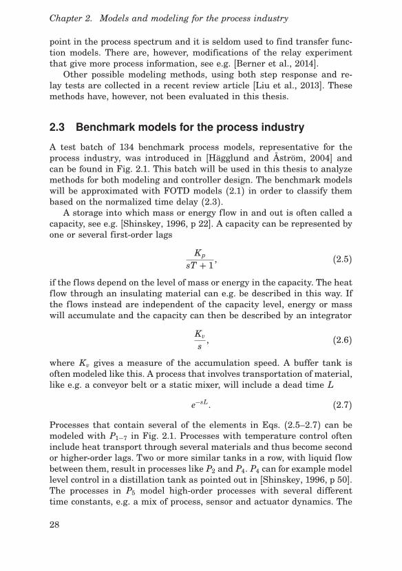
2.3 Benchmark models for the process industry
A test batch of 134 benchmark process models, representative for theprocess industry, was introduced in [Hägglund and Åström, 2004] andcan be found in Fig. 2.1. This batch will be used in this thesis to analyzemethods for both modeling and controller design. The benchmark modelswill be approximated with FOTD models (2.1) in order to classify thembased on the normalized time delay (2.3).A storage into which mass or energy flow in and out is often called a
capacity, see e.g. [Shinskey, 1996, p 22]. A capacity can be represented byone or several first-order lags
Kp
sT + 1, (2.5)
if the flows depend on the level of mass or energy in the capacity. The heatflow through an insulating material can e.g. be described in this way. Ifthe flows instead are independent of the capacity level, energy or masswill accumulate and the capacity can then be described by an integrator
Kv
s, (2.6)
where Kv gives a measure of the accumulation speed. A buffer tank isoften modeled like this. A process that involves transportation of material,like e.g. a conveyor belt or a static mixer, will include a dead time L
e−sL. (2.7)
Processes that contain several of the elements in Eqs. (2.5–2.7) can bemodeled with P1−7 in Fig. 2.1. Processes with temperature control ofteninclude heat transport through several materials and thus become secondor higher-order lags. Two or more similar tanks in a row, with liquid flowbetween them, result in processes like P2 and P4. P4 can for example modellevel control in a distillation tank as pointed out in [Shinskey, 1996, p 50].The processes in P5 model high-order processes with several differenttime constants, e.g. a mix of process, sensor and actuator dynamics. The
28

2.3 Benchmark models for the process industry
P1(s) =e−s
1+ sT ,
T = 0.02, 0.05, 0.1, 0.2, 0.3, 0.5, 0.7, 1,1.3, 1.5, 2, 4, 6, 8, 10, 20, 50, 100, 200, 500, 1000
P2(s) =e−s
(1+ sT)2 ,
T = 0.01, 0.02, 0.05, 0.1, 0.2, 0.3, 0.5, 0.7, 1,1.3, 1.5, 2, 4, 6, 8, 10, 20, 50, 100, 200, 500
P3(s) =1
(s+ 1)(1+ sT)2 ,
T = 0.005, 0.01, 0.02, 0.05, 0.1, 0.2, 0.5, 2, 5, 10
P4(s) =1
(s+ 1)n ,
n = 3, 4, 5, 6, 7, 8
P5(s) =1
(1+ s)(1+α s)(1+α 2s)(1+α 3s) ,
α = 0.1, 0.2, 0.3, 0.4, 0.5, 0.6, 0.7, 0.8, 0.9
P6(s) =1
s(1+ sT1)e−sL1 ,
L1 = 0.01, 0.02, 0.05, 0.1, 0.2, 0.3, 0.5, 0.7, 0.9, 1.0, T1 + L1 = 1
P7(s) =1
(1+ sT)(1+ sT1)e−sL1 , T1 + L1 = 1,
T = 1, 2, 5, 10 L1 = 0.01, 0.02, 0.05, 0.1, 0.3, 0.5, 0.7, 0.9, 1.0
P8(s) =1−α s
(s+ 1)3 ,
α = 0.1, 0.2, 0.3, 0.4, 0.5, 0.6, 0.7, 0.8, 0.9, 1.0, 1.1
P9(s) =1
(s+ 1)((sT)2 + 1.4sT + 1) ,
T = 0.1, 0.2, 0.3, 0.4, 0.5, 0.6, 0.7, 0.8, 0.9, 1.0
Figure 2.1 Test batch of 134 processes representative for the processindustry.
29

Chapter 2. Models and modeling for the process industry
integrating processes in P6 could e.g. model the concentration in a batchwith sensor lag and transportation delay. Right half plane zeros, like thosein P8, could be the result of e.g. boiler water level control or concentrationcontrol in a series of two continuous stirred-tank reactors [Marlin, 1995;Desborough and Miller, 2002]. A mechanical process or a recirculationloop are examples of processes with complex poles, like P9.According to [Shinskey, 1996, p 99]many processes have static gains in
the range Kp = 1− 10. It is reasonable to believe, however, that Kv couldbe a much smaller number e.g. for large tanks. In this thesis both Kp andKv have been set to 1 for the batch. It seems reasonable to believe thatthese two gains will vary randomly from process to process, i.e. similar tothe characteristics of the measurement noise. This is relevant informationsince the noise sensitivity measure used in this thesis depends on thesegains, see Section 3.3.
30

3
Criteria and trade-offs for
PID design
A rational way to design a controller is to derive a process model and acollection of requirements. Constrained optimization can then be appliedto make a trade between often conflicting requirements. Tuning of PIDcontrollers for the process industry is seldom done this way since the effortthat can be devoted to a single loop is severely limited.Requirements typically include specifications on load disturbance at-
tenuation, robustness to process uncertainty, noise sensitivity and set-point tracking. Load disturbance attenuation is a primary concern in pro-cess control where steady-state regulation is a key issue, see [Shinskey,1996], while set-point tracking is a major concern in motion control. Set-point tracking can, however, be treated separately by using a control ar-chitecture having two degrees of freedom, see e.g. [Åström and Hägglund,2005] for more information. Therefore, the focus of this thesis will be onload disturbance attenuation.
3.1 Performance
Load disturbance attenuation will be characterized here by the integratedabsolute error (IAE)
IAE =∞∫
0
pe(t)pdt, (3.1)
for a unit step load disturbance on the process input. The IAE-value isthus equal to the total area under the response, as shown in Fig. 3.1.[Shinskey, 1996, p 17] points out that the IAE is a valuable performancemeasure since it can be related to the economic cost of adding either too
31

Chapter 3. Criteria and trade-offs for PID design
0 5 10 15 20 25-0.1
0
0.1
0.2
0.3
0.4
Controlerror
Time
Figure 3.1 The IAE-value is equal to the shaded area of the load dis-turbance response.
much or too little of a valuable ingredient. Other integral criteria forcontrol performance such as the integrated error (IE)
IE =∞∫
0
e(t)dt, (3.2)
the integrated square error (ISE)
ISE =∞∫
0
e2(t)dt, (3.3)
and the integrated time-weighted absolute error (ITAE)
ITAE =∞∫
0
tpe(t)pdt, (3.4)
have also been suggested by e.g. [McMillan, 1983; Marlin, 1995].When performance is considered, it is important to remember that
not all control loops need optimal performance. The process in Paper Vis a good example of this since the acceptable range for the temperaturecontrol is rather wide.
32

3.2 Robustness
3.2 Robustness
As stated in Section 1.3, it is very important to ensure that all plantprocesses are safe and stable around the set-point. For this reason, theprimary goal of many PID design methods is to secure the robustness ofthe closed-loop system, i.e. to keep good margins to the point of instability.The phase margin and the gain margin are classical robustness mea-
sures that are still used today [Sanchis et al., 2010; Romero et al., 2011].See [Åström and Hägglund, 2005, pp 104–105] for definitions.According to e.g. [Åström and Hägglund, 2005, pp 112–116] and [Zhou
and Doyle, 1998, pp 142–143] robustness can be captured by the sensitiv-ity function, S(s), and the complementary sensitivity function, T(s), seeEqs. (1.4–1.5). The maximum values of these functions
pS(iω )p ≤ Ms, pT(iω )p ≤ Mt, ∀ω ∈ R+, (3.5)
i.e. the H∞-norms, will be used in this thesis as robustness constraintson the closed-loop system. Note that ω is the frequency in [rad/s] and R+denotes the set of all non-negative real numbers. As shown in [Åström andHägglund, 2005, pp 116–117], this corresponds to the open-loop Nyquistcurve of P(iω )C(iω )F(iω ) not entering the Ms- or Mt-circles shown inFig. 3.2. The circles expand with decreasing values of Ms and Mt, resultingin greater closed-loop robustness. Values of Ms and Mt ranging between1.2 and 2.0 are said to give reasonable robustness [Åström and Hägglund,2005, p 127] and correspond to gain margins between 6 and 2, as well asphase margins between 49○ and 29○. The measure
Mst = max(pS(iω )p, pT(iω )p), ∀ω ∈ R+ (3.6)
will also be used here to quantify the robustness of the closed-loop systemgiven some controller C(s).The so called M -circle is the smallest circle that encircles the Ms and
Mt-circles and it is sometimes used as an alternative robustness criteria,see e.g. [Hägglund and Åström, 2004]. A few other robustness measurescan be found in e.g. [Alfaro, 2007; Larsson and Hägglund, 2009; Hansen,2012].
3.3 Noise sensitivity
Large control signal activity generated by measurement noise could causeundesirable actuator wear and tear. The impact of the transfer functionfrom measurement noise to control action, Sc(s), depends on many fac-tors, with the controller parameters and low-pass filter being particularly
33

Chapter 3. Criteria and trade-offs for PID design
-4 -3 -2 -1 0 1-2
-1
0
1
2
Imaginaryaxis
Real axis
Figure 3.2 The robustness constraints in (3.5) are fulfilled if the open-loop Nyquist curve (solid) does not enter the Ms-circle (dashed) or theMt-circle (dash-dotted).
important. As with both performance and robustness, there are severalpossible measures of the closed-loop noise sensitivity. [Garpinger, 2009]and Paper V use the ratio between control signal and measurement noisevariance
σ 2uσ 2n
≤ Vk, (3.7)
to constrain the impact of the measurement noise. σu denotes the stan-dard deviation of the control signal due to noise and σ n is the standarddeviation of the noise itself. A drawback with this measure is that oneneeds information about the noise profile, e.g. the spectral density, in or-der to calculate it. For this reason, the more recent Paper IV instead usesthe H2 norm of Sc(s)
qSc(s)q2 ≤ κu, (3.8)
to constrain the noise sensitivity. This condition is also used by e.g. [Lars-son and Hägglund, 2011]. Assuming continuous-time white Gaussian mea-surement noise with unit spectral density, qSc(s)q2 can be derived using
34

3.4 Constrained optimization of PID controllers
the integral formula
qSc(s)q2 =
√
√
√
√
√
12π
∞∫
−∞
pSc(iω )p2dω . (3.9)
This equation will mainly be used for the purpose of controller analysis inthis thesis. For control of real processes where the noise characteristicsis typically different, it makes more sense to use σu as the measure ofnoise sensitivity. However, one of the biggest advantages with the PIDdesign procedure proposed in Paper IV, is that there is no need to deriveσu explicitly for real processes.Two other options would be to use either the H∞-constraint
qSc(s)q∞ ≤ cu, (3.10)see e.g. [Kristiansson and Lennartson, 2006; Micić and Mataušek, 2014],or the total variation (TV) of the control signal
TV =∞∑
i=1pui+1 − uip, (3.11)
where pui+1−uip denotes the control signal change between two consecutivesamples, see e.g. [Skogestad, 2003].
3.4 Constrained optimization of PID controllers
PID control studies seldom treat more than one or two tuning criteria forcontroller design. Taking all three criteria of performance, robustness andnoise sensitivity into consideration, one can formulate several differentconstrained optimization problems. The one that will be the main focusof this thesis is
minimizeK ,Ti,Td,T f∈R+
∞∫
0
pe(t)pdt,
subject to pS(iω )p ≤ Ms,pT(iω )p ≤ Mt, ∀ω ∈ R
+,
qSc(s)q2 ≤ κu,
(3.12)
with the cost function and constraints as defined in Eqs. (3.1), (3.5) and(3.8). This optimization problem can be used to design any of the con-trollers C(s) given in Eqs. (1.11–1.13) as well as the filters in Eqs. (1.17–1.18). However, the non-convexity of this optimization problem makes itdifficult to solve directly.
35

4
PID design methods
In this chapter we distinguish between PID design based on tuning rulesand optimization. Tuning rules are a set of formulas from which onecan determine the controller parameters, and they typically depend onthe parameters of some specific process model, e.g. FOTD or SOTD.In optimization-based methods, the controller parameters are insteadderived from the solution to an optimization problem like (3.12), alsogiven some model of the process. The aim of tuning rules is thus tofind universal relations between model and controller parameters, whileoptimization-based design treats each process model individually.
4.1 Tuning rules
A good PID tuning method should both be fast and easy to carry out forthe large number of control loops in a factory. This has led to the greatpopularity of formula-based tuning rules. A measure of this popularity isgiven by the book [O’Dwyer, 2009], in which there are 1,730 PI and PIDtuning rules collected. Some of the most commonly used tuning rules arecompared in this thesis (see Papers I and III), both with respect to eachother and optimal PID design. Another example of a study that comparesseveral different tuning rules is [Lin et al., 2008].
The Ziegler-Nichols methods
During the second world war, [Ziegler and Nichols, 1942] presented twomethods for design of P, PI and PID controllers that have received con-siderable attention. The step response method uses only two parameters,Kv and L. These are determined from a step response where Kv is thesteepest slope and L is the intersection of the steepest tangent with thetime axis. L is therefore the same as in the 63%-rule, see Section 2.2. The
36

4.1 Tuning rules
step response method gives the PI controller parameters
K = 0.9KvL
, Ti = 3L. (4.1)
The Ziegler-Nichols frequency response method is based on a closed-looptest with a P controller. The proportional gain is increased until the pro-cess is on the border to instability. This proportional gain is called the ul-timate gain, Ku, and the oscillation period is called the ultimate period,Tu. The frequency response method is tuned to give quarter amplitudedamping of load disturbance responses and is given by
K = 0.4Ku, Ti = 0.8Tu. (4.2)
The Ziegler-Nichols methods are included in this thesis only for historicalreasons. Several studies have concluded that the tuning methods are notsuited for industrial practice, but they are still quite frequently used. Forexample, [Bialkowski, 1993] states that
"Most trade schools deal with the loop tuning issue by teaching
the Ziegler Nichols quarter-amplitude-decay method as the only
reasonable fallback position. Unfortunately, for the pulp and
paper industry, this method is very oscillatory and is one of the
reasons for the destabilization of paper uniformity."
Internal model control
IMC is based on the configuration in Fig. 4.1 where P(s) is the pro-cess, Pm(s) is the process model and CIMC(s) is the internal model con-troller. The process model is separated into two parts, one minimumphase part P−(s) and a non-minimum phase part P+(s) such that Pm(s) =P−(s)P+(s). The IMC controller is then defined as CIMC(s) = P−1− (s) f (s)e.g. with
f (s) = 1(Tcls+ 1)r
, (4.3)
where the integer r is set such that the IMC controller is proper. Assumingthat the process model is perfect and minimum phase, i.e. P(s) = Pm(s) =P−(s), the closed-loop system from R(s) to Y(s) becomes T(s) = f (s). Tclcan thus be viewed as a tuning parameter adjusting the speed of theclosed-loop system. The IMC configuration in Fig. 4.1 can be transformedto the closed-loop system in Fig. 1.1 by the formula
C(s) = CIMC(s)1− Pm(s)CIMC(s)
= P−1− (s)f−1(s) − P+(s)
. (4.4)
37

Chapter 4. PID design methods
Σ
Σ
Σ
e u y
P(s)CIMC(s)
−Pm(s)
d
r z
−1
Figure 4.1 The IMC configuration.
[Rivera et al., 1986] points out that most process models used in industrialapplications lead to IMC controllers on the PID form. Based on differentforms of process models, a large number of IMC PID tuning rules arepresented in this paper [Rivera et al., 1986, Table 1]. These formulas are,however, known to give poor performance to e.g. input load disturbanceson lag dominated processes since the slow process pole is still presentin this response. Some modifications to IMC-based PID are presented ine.g. [Lee et al., 1998; Shamsuzzoha and Lee, 2007; Vilanova, 2008]. In thisthesis, however, two other IMC-related methods are used for PID designcomparison, namely Lambda tuning and SIMC.
Lambda tuning
Lambda tuning originates from early computer control [Dahlin, 1968;Higham, 1968], was rediscovered in connection with the development ofIMC PID [Rivera et al., 1986], and is today widely adopted in the industry,see e.g. [Sell, 1995; Bialkowski, 1996; Forsman, 2005]. Modeling is typi-cally based on step responses, and an FOTD model can be obtained usingfor example the 63%-rule. The desired closed-loop time constant to a set-point change, Tcl, is used as a tuning parameter. This parameter admitsa compromise between performance and robustness where low values onTcl give aggressive control, while higher values give smooth control. Inthe original paper [Dahlin, 1968], 1/Tcl was called λ , which explains thename of the tuning method. For PI control the tuning formulas are
K = T
Kp(Tcl + L), Ti = T , (4.5)
38

4.1 Tuning rules
and for series form PID they are
K ′ = T
Kp(Tcl + L), T ′i = T , T ′d =
L
2, (4.6)
given the notations from (1.12), (1.14) and (2.1). These two tuning formu-las can be derived directly from rules D and F in [Rivera et al., 1986, Table1] using either a first-order Taylor expansion (PI) or a first-order Padéapproximation (PID) of the time delay. The Lambda tuning rules inheritthe problem with sluggish load disturbance responses from IMC tuningfor processes with lag-dominated dynamics. There are several suggestionsfor choosing Tcl, some of which can be found in [Sell, 1995; Bialkowski,1996; Janvier and Bialkowski, 2005]. [Janvier and Bialkowski, 2005] alsogives instructions for Lambda tuning modifications of integrating andlag-dominated processes. In this thesis, however, Tcl will be chosen pro-portional to the process time constant T .
Skogestad’s methods
[Skogestad, 2003] introduced modifications of the Lambda tuning methodcalled SIMC, that improves performance especially for lag-dominant pro-cesses. The FOTD model is obtained by model reduction of a high-orderprocess model using the half-rule. The proportional gain K is chosen asin (4.5) and the integral time as
T ′i = min(T , 4(Tcl + L)). (4.7)
This choice avoids cancellation of a slow process pole by a controller zerowhen T > 4(Tcl + L). Furthermore, Skogestad recommends PID controlmainly for processes with dominant second-order dynamics, which canbe modeled using (2.2). In this case, T is replaced by the largest timeconstant T1 in (4.5) and (4.7). The derivative time is set to
T ′d = T2. (4.8)
Notice that the PID series form is used. Unlike the original Lambda tun-ing, the desired closed-loop time constant Tcl is chosen as a factor of theapparent time delay L. Skogestad recommends Tcl = L as the primarychoice which typically gives a sensitivity close to Ms = 1.6. Less aggres-sive tuning is obtained for larger values of Tcl and can be found throughselection of an upper limit on the controller gain, see [Skogestad, 2006].A modified version of SIMC PI control, here called SIMC+, was in-
troduced in [Skogestad and Grimholt, 2012] to improve performance fordelay-dominated systems where the original SIMC rule typically results
39
Chapter 4. PID design methods
in controllers with too low proportional gain. The PI parameters wereinstead chosen as
K = T + L/3Kp(Tcl + L)
, Ti = min(T + L/3, 4(Tcl + L)). (4.9)
For delay-dominated and balanced processes the integral gain is the sameas for SIMC, while the proportional gain K and integral time Ti arelarger than for SIMC. Recently [Grimholt and Skogestad, 2013], made yetanother extension to the SIMC rules that also designs PID controllers forFOTD processes. This new study is, however, not considered in this thesis.
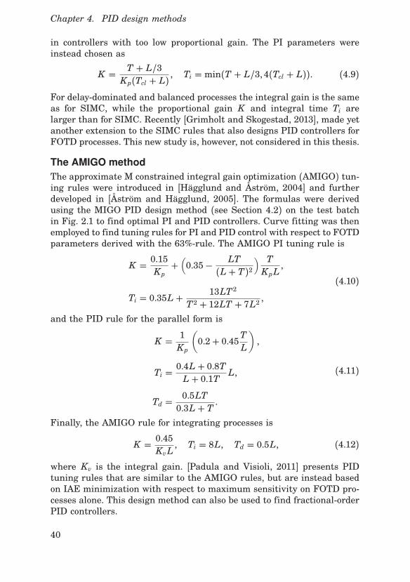
The AMIGO method
The approximate M constrained integral gain optimization (AMIGO) tun-ing rules were introduced in [Hägglund and Åström, 2004] and furtherdeveloped in [Åström and Hägglund, 2005]. The formulas were derivedusing the MIGO PID design method (see Section 4.2) on the test batchin Fig. 2.1 to find optimal PI and PID controllers. Curve fitting was thenemployed to find tuning rules for PI and PID control with respect to FOTDparameters derived with the 63%-rule. The AMIGO PI tuning rule is
K = 0.15Kp
+(
0.35− LT
(L + T)2) T
KpL,
Ti = 0.35L +13LT2
T2 + 12LT + 7L2 ,(4.10)
and the PID rule for the parallel form is
K = 1Kp
(
0.2+ 0.45TL
)
,
Ti =0.4L + 0.8TL + 0.1T L,
Td =0.5LT0.3L + T .
(4.11)
Finally, the AMIGO rule for integrating processes is
K = 0.45KvL
, Ti = 8L, Td = 0.5L, (4.12)
where Kv is the integral gain. [Padula and Visioli, 2011] presents PIDtuning rules that are similar to the AMIGO rules, but are instead basedon IAE minimization with respect to maximum sensitivity on FOTD pro-cesses alone. This design method can also be used to find fractional-orderPID controllers.
40
4.2 Optimization-based methods
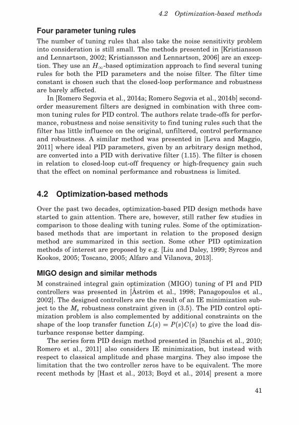
Four parameter tuning rules
The number of tuning rules that also take the noise sensitivity probleminto consideration is still small. The methods presented in [Kristianssonand Lennartson, 2002; Kristiansson and Lennartson, 2006] are an excep-tion. They use an H∞-based optimization approach to find several tuningrules for both the PID parameters and the noise filter. The filter timeconstant is chosen such that the closed-loop performance and robustnessare barely affected.In [Romero Segovia et al., 2014a; Romero Segovia et al., 2014b] second-
order measurement filters are designed in combination with three com-mon tuning rules for PID control. The authors relate trade-offs for perfor-mance, robustness and noise sensitivity to find tuning rules such that thefilter has little influence on the original, unfiltered, control performanceand robustness. A similar method was presented in [Leva and Maggio,2011] where ideal PID parameters, given by an arbitrary design method,are converted into a PID with derivative filter (1.15). The filter is chosenin relation to closed-loop cut-off frequency or high-frequency gain suchthat the effect on nominal performance and robustness is limited.
4.2 Optimization-based methods
Over the past two decades, optimization-based PID design methods havestarted to gain attention. There are, however, still rather few studies incomparison to those dealing with tuning rules. Some of the optimization-based methods that are important in relation to the proposed designmethod are summarized in this section. Some other PID optimizationmethods of interest are proposed by e.g. [Liu and Daley, 1999; Syrcos andKookos, 2005; Toscano, 2005; Alfaro and Vilanova, 2013].
MIGO design and similar methods
M constrained integral gain optimization (MIGO) tuning of PI and PIDcontrollers was presented in [Åström et al., 1998; Panagopoulos et al.,2002]. The designed controllers are the result of an IE minimization sub-ject to the Ms robustness constraint given in (3.5). The PID control opti-mization problem is also complemented by additional constraints on theshape of the loop transfer function L(s) = P(s)C(s) to give the load dis-turbance response better damping.The series form PID design method presented in [Sanchis et al., 2010;
Romero et al., 2011] also considers IE minimization, but instead withrespect to classical amplitude and phase margins. They also impose thelimitation that the two controller zeros have to be equivalent. The morerecent methods by [Hast et al., 2013; Boyd et al., 2014] present a more
41

Chapter 4. PID design methods
general framework of convex-concave optimization which can be solvedvery quickly, but it is still based on IE minimization with robustnessconstraints. [Grimholt and Skogestad, 2015], on the other hand, presentsa fast algorithm for minimization of input and output disturbance IAEwith respect to the robustness constraints in (3.5). This new method isthus very similar to the next one presented here.
SWORD
A MATLAB®-based software tool for robust PI and PID design is pre-sented in Paper II. This tool extends the one presented in [Nordfeldt andHägglund, 2006], and solves a modified version of Eq. (3.12) without thenoise sensitivity constraint. The optimization problem is
minimizeK ,Ti,Td∈R+
∞∫
0
pe(t)pdt,
subject to pS(iω )p ≤ Ms,pT(iω )p ≤ Mt, ∀ω ∈ R
+,
pS(iω s)p = Ms, and/orpT(iω t)p = Mt,
(4.13)
where ω s are frequencies for which the open-loop frequency response istangent to the Ms-circle and vice versa for ω t and the Mt-circle. Eitherω s or ω t could be an empty set, but not simultaneously. As a direct resultof these additional equality constraints, at least one of the inequalityconstraints will be active, thus forcing the solution to have contact with atleast one of the Ms- and Mt-circles. This makes the optimization problemeasier to solve than the problem with only inequality constraints. Thedrawback is that there could be a controller with greater robustness thatyields better performance. Several studies by [Garpinger, 2009; Grimholtand Skogestad, 2012; Garpinger et al., 2014] do, however, indicate that thesolution to the optimization problem (4.13) is, in most cases, optimal alsowithout equality constraints just as long as the robustness is reasonablewith Ms and Mt roughly below 1.8. The low-pass filter time constant, T f , isfixed in this optimization problem such that the controllers are designedfor the process and filter combination P(s)F(s). This design method iscalled SWORD (Software-based optimal robust design) and it needs astable linear process model as well as specified values of Ms, Mt and T f towork. A more detailed description of the program is given in Paper II. Alsonote that the tool can easily be modified to deal with e.g. discrete-timePID control, other performance measures and different low-pass filterconfigurations. The software tool is freely available at:
42

4.2 Optimization-based methods
http://www.control.lth.se/project/PID
Other similar design methods can be found in [Oviedo et al., 2006;Harmse et al., 2009; Sadeghpour et al., 2012], which present software toolsthat can be readily used for constrained optimization of the PID parame-ters. This collection of methods will here be referred to as Software-basedoptimal design methods. Notice that MATLAB® has a PID optimizationtool of its own [MathWorks®, 2015].
Four parameter optimization methods
The optimization-based methods presented so far, except [Panagopouloset al., 2002], have in common that performance and robustness are theirmain focus. They exploit constrained optimization, but they do not ex-plore the noise sensitivity problem. Studies by [Šekara and Mataušek,2009; Larsson and Hägglund, 2011; Micić and Mataušek, 2014] show howconstrained optimization can be used to design PID controllers and noisefilters of different orders. The methods do, however, only describe howthe optimization can be carried out, and they do not present any softwaretools for solving their respective optimization problems.The method for design of PID controllers and noise filters proposed in
Paper IV is based on the method from [Garpinger, 2009]. The original ideauses the MATLAB® toolbox presented in the previous subsection to solve aconstrained optimization problem for the design of robust PID controllers.The noise filter time constant is fixed each time a new controller is de-signed and the closed-loop noise sensitivity is then constrained throughrepeated PID design, similar to the method presented in [Panagopouloset al., 2002]. With this approach there is no need to keep the performanceclose to the unfiltered, nominal, case. An increase of the filter time con-stant does not affect the robustness as it would in the earlier mentionedmethods by [Romero Segovia et al., 2014a; Romero Segovia et al., 2014b;Kristiansson and Lennartson, 2002; Kristiansson and Lennartson, 2006].Noise sensitivity is measured by the variance gain from measurementnoise to control signal (see Eq. 3.7), and Simulink® simulations are usedto calculate this measure by the use of process noise data.
43

5
Friction stir welding
The author of this thesis has had the opportunity to work on the tempera-ture control of an industrial friction stir welding (FSW) process. While thegiven machine is not part of any process industry, it is still a good exam-ple of a process where PID control is sufficient. One of the measurementsignals used in the final cascade controller also includes a lot of noise,which makes the process suitable for analysis of the proposed control de-sign technique. The first controller tuning made for the FSW process isdescribed in Paper V and uses the design method proposed in the author’slicentiate thesis [Garpinger, 2009]. A supplement has been added to Pa-per V in this thesis, to show that the design procedure proposed in PaperIV is better to use.
5.1 Background
FSW is a thermo-mechanical solid-state process that was invented in 1991at The Welding Institute (TWI) [Thomas et al., 1991]. A rotating non-consumable tool, consisting of a tapered probe and shoulder, is plungedinto the weld metal and traversed along the joint line, see Fig. 5.1. Fric-tional heat is generated between the tool and the weld metal, causingthe metal to soften, normally without reaching the melting point, and al-lowing the tool to traverse the joint line. The three most common inputparameters are (see Fig. 5.1)
1. Tool rotation rate
2. Welding speed along the joint
3. Axial force
Temperature control could be an important part of the FSW process if ithas non-uniform thermal boundary conditions or if it is used on a material
44

5.2 FSW of thick copper canisters for nuclear waste
Figure 5.1 Illustration of the friction stir welding process.
with a smaller allowed temperature range, the so-called process window.If the welding temperature gets too high for a longer period of time, thereis a risk for probe fracture. Similarly, too low temperatures may result indiscontinuities in the weld. A previous study by [Cederqvist et al., 2008]has shown that the rotation rate is the best suited control signal for weldtemperature control and is used here.As of today, most friction stir welds are made on plates with rather
uniform thermal boundary conditions. For this reason, there are currentlyonly a small, although growing, amount of FSW applications using tem-perature control. [Fehrenbacher et al., 2008] have approached closed-loopcontrol of the welding temperature by manipulation of the welding speedand more recently by adjusting the tool rotation rate [Fehrenbacher et al.,2010]. Another study [Mayfield and Sorensen, 2010] suggests a cascadedcontrol strategy similar to that previously presented in [Cederqvist et al.,2009] and in Paper V. Recently, there have been two more studies ontemperature control, see [De Backer et al., 2014; Ross, 2014].The need for reliable control of the welding temperature should in-
crease as FSW is used on metals like titanium and steels. In addition,more complex geometries of welding objects will result in non-uniformthermal boundary conditions and thus also a need for temperature con-trol.
5.2 FSW of thick copper canisters for nuclear waste
The Swedish Nuclear Fuel and Waste Management Company (SKB) plansto join at least 12,000 lids and bases to the extruded copper tubes con-taining Sweden’s nuclear waste, using FSW. The canisters produced (5m height, 1 m diameter) are a major component of the Swedish system
45

Chapter 5. Friction stir welding
T
Figure 5.2 The cascaded control structure proposed for the FSW process.
for managing and disposing nuclear waste. They will be stored in theSwedish bedrock and must remain intact for 100,000 years. A corrosionbarrier of 5 cm thick copper and a cast iron insert are used to meet thisrequirement.The friction stir welding machine currently used to seal the copper
canisters measures the welding temperature [○C] and the torque [Nm]required to maintain the tool rotation rate. Another important variableis the power input [kW] which is proportional to the tool rotation ratemultiplied with the torque. [Cederqvist et al., 2008] showed that the powerinput is well correlated to the welding temperature.Of all process outputs, the welding temperature is the most crucial one
to control. It is, therefore, very important to keep the temperature withinthe process window, which is roughly between 790 and 910○C for FSWon the copper canisters, when measured inside the probe. Several aspectsof the welds make the temperature challenging to control. Depending onthe position of the tool, a full weld cycle can be divided into five separatesequences each with challenges of different nature. For example, the start-up typically contain a lot of fast and high-magnitude torque disturbances.Other disturbances are caused either by the tool moving in and out ofpreheated areas or by greater heat conduction at the joint line comparedto the lid. Each of these disturbances has to be counteracted to make surethe temperature stays within the process window.
5.3 PID design for an FSW process
A cascaded control strategy seems ideal for the characteristics of thisspecific FSW application with its fast torque disturbances, and slowertemperature counterparts. It was, therefore, decided to use the controllerstructure displayed in Fig. 5.2. The process has been divided into twosubsystems. Process G1 holds the dynamics from the tool rotation rate,
46

5.3 PID design for an FSW process
u (rpm), to the power input, P (kW). Step response modeling resulted inthe process model
G1(s) = 0.12 ⋅4.62
s2 + 2 ⋅ 0.8 ⋅ 4.6s+ 4.62 . (5.1)
This system mainly holds the servo characteristics of the spindle motorthat drives the probe. The outer process, G2, on the other hand, describeshow the power input is related to the probe temperature, T (○C). Thisprocess model,
G2(s) =11.6
(7s+ 1)2 e−5s, (5.2)
was also derived using step response modeling as described in Paper V.The process was originally controlled by two PI controllers, C1 and C2,
which were sufficient to keep the temperature within the process window,see Paper V. The design procedure was based on the one proposed in[Garpinger, 2009], but no low-pass filters, Cf1 or Cf2 , were used in thecontrol solution. Since Paper V was written, the PID design procedure hasbeen updated, see Paper IV. In the Supplement to Paper V it is shown howan inner I controller and outer PID controller, with low-pass filter Cf2(s),can be derived using the updated design procedure in order to improvethe temperature control at the joint line.
47

6
Thesis contributions
6.1 Thesis objectives
In industry, PID control is by far the most common control strategy andmore advanced control techniques are often rejected due to lack of timeand personnel with the required knowledge. In an effort to present PIDtuning methods for the industry, most PID researchers strive to developtuning rules which can easily be used by practitioners. This has led toseveral methods that are good at finding robust PI controllers. However,these methods often fail to design controllers with respect to optimal per-formance as well as noise sensitivity.The objectives of this thesis are to propose new tools for design and
analysis of PID controllers. These should show advantages of tuning basedon constrained optimization as well as how and when to use it. This isa standpoint that recognizes both the academic efforts on constrainedoptimization and the industry in which the PID algorithm is likely toremain for many years to come.
6.2 Contributions
The low order of the PID controller makes it easier to analyze, with respectto the different controller criteria, than more complex control strategies.This property is exploited in Paper I, where new trade-off plots are pre-sented. Performance and robustness level curves are drawn as functionsof the PID parameters. This is a tool that can provide tuning insight andintuition for practitioners as well as students. It is also used to showweaknesses and strengths of different PI tuning rules.The trade-off plots are also used to show the set of optimal controllers
for different robustness values. This set can be derived directly by theMATLAB®-based software design method which was briefly mentionedin Section 4.2 (i.e. SWORD). It is thoroughly described in Paper II. As far
48

6.2 Contributions
as the author of this thesis knows, this is the only freely available PIDdesign tool that minimizes IAE with respect to robustness constraints.The usefulness of the software is demonstrated in Papers III–V, both forcontroller analysis and PID design on real processes. So far, the programhas mainly been used for academic purposes, but similar software-basedoptimal design methods should be commercially viable in the future. How-ever, as shown in Paper III, it is important to find a modeling method thatworks well together with the optimal PID design. FOTD models based onthe 63%-rule (see Section 2.2) are e.g. not good enough to use togetherwith SWORD neither for PI nor PID control and several common tuningrules share this weakness, at least in the PID case. It is shown that amoderate amount of process knowledge, concentrated around single phaseangles, is enough to provide both PI and PID control close to optimal.Knowing that the closed-loop robustness variation can be decreased com-pared to other tuning methods, it is also pointed out that Ms and Mt canbe increased to improve performance even further.The design method presented in Paper IV shows how SWORD can be
used to find optimal or near-optimal PID controllers also with respectto control signal noise sensitivity. The procedure uses the low-pass filtertime constant T f and the integral gain ki as tuning variables to create aset of PID, PI and I controllers. For example, Bode magnitude plots of aset of 17 PID, 7 PI, and 7 I controllers, derived for the balanced process,
P(s) = 1(s+ 1)4 , (6.1)
with Ms = Mt = 1.4, are shown in in Fig. 6.1. Such a set of controllerscan also be used to slow down the closed-loop system if it is deemedtoo fast. In Paper IV, performance and noise sensitivity trade-off curvesare plotted for different robustness levels and give insight into designwith respect to all three criteria. The article also presents a new methodfor quantifying the benefit of the derivative part, by comparing optimalPI and PID controllers with the same robustness and noise sensitivityconstraints. Besides these major contributions, which the thesis authorbelieve are novel, the paper ends with a comparison of tuning rules andsoftware-based optimal design. The main conclusions from this compari-son are that even though tuning rules are a good tool for present use inindustry, software-based optimal tuning has a greater research potential.In Paper V, the SWORD method is used to design two PI controllers
in a cascade-loop for control of a friction stir welding process. As far asthe thesis author knows, this is the first time that a cascade controllerhas been systematically designed and applied to the temperature con-trol problem of an FSW process. Since the PID design procedure usedin Paper V is older than the one presented in Paper IV, a supplement
49

Chapter 6. Thesis contributions
10-3
10-2
10-1
100
101
102
103
10-3
10-2
10-1
100
101
102
103
pC(iω)p
ω (rad/s)
Figure 6.1 Bode magnitude plots of a set of PID (blue), PI (green), andI controllers (red), with Ms = Mt = 1.4, derived for the balanced process(6.1).
has been added just after the main paper to show the improvements ofthe updated method. The results also give some nice insights about thenoise content of the control signal showing that PI controllers should beused together with a low-pass filter, at least in this application. Besidesthe design of PID controllers, Paper V also contributes with strategiesfor control during the start and end of the welds, a task that presentsmuch greater challenges than the control during the joint line sequence.One should also remember that for this specific FSW process, the choicesof cascade control and strategies during start-up are much more crucialfor the overall temperature control than the choices of parameters for theindividual PID controllers. For the sake of the thesis, however, one couldinstead view the FSW process as part of e.g. a chemical factory. If allcontrollers of the factory were optimized like this single process, it wouldbe reasonable to expect synergy effects benefiting the factory as a whole.Unfortunately, the level of such benefits is rather difficult to predict andlikely part of the reason why optimal PID control has not already beendeveloped in the industry.
50

6.3 Visions and future work
6.3 Visions and future work
In this thesis, it is suggested that software-based optimal PID designmethods are the future. The future, however, is not here yet, and thequestion is what is missing to fulfill the prediction. The most importantkey still missing is a modeling method that is tailor made for optimalPID control. Some desired properties of such a method have already beensuggested. It should ideally be as fast as possible and therefore providejust the process information that is absolutely necessary for the controldesign. Closed-loop identification experiments, like relay tests, are pre-ferred, since they are less sensitive to disturbances than their open-loopcounterparts. A reasonable approach would be to first develop somethingthat works for PI control and then move on to more general alternatives.The software behind the SWORD method is just one suggestion of how
such a tool could work, and some improvements are necessary before theproposed design procedure from Paper IV can be employed in industry. Forexample, it would be desirable to obtain faster solutions to the optimiza-tion problem. That way it would be possible to quickly determine a wholeset of PID controllers, both with respect to noise sensitivity and robust-ness. A possible way to speed up the solver is to simplify the optimizationproblem even further. What matters is that the software reliably providesPID controllers and low-pass filters that are decently close to optimal,with at least one robustness constraint (e.g. Ms).Experienced control engineers are probably able to use optimization-
based design techniques as stand-alone methods. But in order to attracta broader audience and to speed up controller tuning, they should ideallybe part of future autotuners together with the desired modeling method.One suggestion is to let modeling experiments be run by a PLC (Pro-grammable Logic Controller) or DCS (Distributed Control System), whilesystem identification and optimal PID design could be handled by an ex-ternal unit, like a laptop or tablet computer. The autotuning could thenbe scheduled to run either periodically by an operator or when changeshave been made to the process. This routine should preferably be reliableenough to use without the need of careful supervision.There should be plenty of possibilities to add new interesting features
to future versions of the SWORD software. For example, it would be de-sirable to add optimization of other PID and filter forms, like the seriesform (1.14) and the derivative filter (1.15). It should also be possible tochange the cost function to e.g. minimize ISE (3.3) or ITAE (3.4), bothwith respect to input and output disturbances. In industrial applicationsit is important to have a strategy for set-point changes, and the final soft-ware should thus include some options to design the reference weightsor a reference filter. For educational purposes, it seems like a good idea
51

Chapter 6. Thesis contributions
to combine the optimal PID control design software with functions frompedagogic software tools, like the one presented in [Guzman et al., 2008].Finally, it is important that software-based optimal PID design meth-
ods are tested on more industrial applications and that their functionsare discussed together with experienced control engineers. This will helpfacilitate the acceptance of such methods in the industry.
52

Bibliography
Alfaro, V. M. (2007). “PID controllers’ fragility”. ISA transactions 46:4,pp. 555–559.
Alfaro, V. M. and R. Vilanova (2013). “Performance and Robustness Con-siderations for Tuning of Proportional Integral/Proportional IntegralDerivative Controllers with Two Input Filters”. Industrial & Engineer-ing Chemistry Research 52:51, pp. 18287–18302.
Ang, K. H., G. Chong, and Y Li (2005). “PID Control System Analysis,Design and Technology”. IEEE Transactions on Control Systems Tech-nology 13:4, pp. 559–576.
Åström, K. J. and T. Hägglund (2005). Advanced PID Control. ISA – TheInstrumentation, Systems, and Automation Society, Research TrianglePark, NC.
Åström, K. J., H. Panagopoulos, and T. Hägglund (1998). “Design ofPI Controllers based on Non-Convex Optimization”. Automatica 34:5,pp. 585–601.
Berner, J., K. J. Åström, and T. Hägglund (2014). “Towards a New Gener-ation of Relay Autotuners”. In: 19th IFAC World Congress. Cape Town,South Africa.
Bialkowski, W. L. (1993). “Dreams versus reality: A view from both sidesof the gap”. Pulp & Paper Canada 94:11, pp. 19–27.
Bialkowski, W. L. (1996). “Control of the Pulp and Paper Making Process”.In: Levine, W. S. (Ed.). The Control Handbook. CRC Press, Inc, BocaRaton, Florida. Chap. 72, pp. 1219–1242.
Boyd, S., M. Hast, and K. J. Åström (2014). “MIMO PID Tuning via It-erated LMI Restriction”. Unpublished manuscript. URL: https://web.
stanford.edu/~boyd/papers/mimo_pid_tuning.html.
Buckbee, G. (2002). “Poor Controller Tuning Drives Up Valve Costs”. Con-trol Magazine, pp. 67–77.
53

Bibliography
Cederqvist, L., C. D. Sorensen, A. P. Reynolds, and T. Öberg (2008). “Im-proved process stability during friction stir welding of 5 cm thick cop-per canisters through shoulder geometry and parameter studies”. Sci-ence and Technology in Welding and Joining 46:2, pp. 178–184.
Cederqvist, L., R. Johansson, A. Robertsson, and G. Bolmsjö (2009).“Faster Temperature Response and Repeatable Power Input to aid Au-tomatic Control of Friction Stir Welded Copper Canisters”. In: FrictionStir Welding and Processing V. San Francisco, USA.
Dahlin, E. B. (1968). “Designing and tuning digital controllers”. Instru-ments and Control Systems 41:6, pp. 77–83.
De Backer, J., G. Bolmsjö, and A.-K. Christiansson (2014). “Tempera-ture control of robotic friction stir welding using the thermoelectriceffect”. The International Journal of Advanced Manufacturing Tech-nology 70:1-4, pp. 375–383.
Desborough, L. and R. Miller (2002). “Increasing Customer Value of In-dustrial Control Performance Monitoring-Honeywell’s Experience”. In:AIChE Symposium Series, Number 326 (Volume 98), pp. 169–189.
Ender, D. B. (1993). “Process Control Performance: Not as Good as youThink”. Control Engineering 40:10, pp. 180–190.
Ender, D. B. (2001). “Regulatory Control is the Foundation for AdvancedProcess Control”. Control Engineering.
Fehrenbacher, A., F. E. Pfefferkorn, M. R. Zinn, N. J. Ferrier, and N.A. Duffie (2008). “Closed-loop Control of Temperature in FrictionStir Welding”. In: 7th International Friction Stir Welding Symposium.Awaji Island, Japan.
Fehrenbacher, A., N. A. Duffie, N. J. Ferrier, M. R. Zinn, and F. E. Pf-efferkorn (2010). “Temperature measurement and closed-loop controlin friction stir welding”. In: 8th International Friction Stir WeldingSymposium. Timmendorfer Strand, Germany.
Forsman, K. (2005). Reglerteknik för processindustrin. Studentlitteratur,Lund, Sweden.
Franklin, G. F., J. D. Powell, and A. Emami-Naeini (2010). Feedback Con-trol of Dynamic Systems. 6th Edition. Pearson, Upper Saddle River,NJ.
Garpinger, O. (2009). Design of Robust PID Controllers with ConstrainedControl Signal Activity. Licentiate Thesis ISRN LUTFD2/TFRT--3245--SE. Department of Automatic Control, Lund University, Swe-den.
Garpinger, O., T. Hägglund, and K. J. Åström (2014). “Performance androbustness trade-offs in PID control”. Journal of Process Control 24:5,pp. 568–577.
54
Bibliography
Gonzales, R. (2012). “Future Perspectives of PID Control - Panel Session”.In: IFAC Conference on Advances in PID Control. Brescia, Italy.
Grimholt, C. and S. Skogestad (2012). “Optimal PI-Control and Verifica-tion of the SIMC Tuning Rule”. In: IFAC Conference on Advances inPID Control. Brescia, Italy.
Grimholt, C. and S. Skogestad (2013). “Optimal PID-Control on First Or-der Plus Time Delay Systems & Verification of the SIMC Rules”. In:10th IFAC International Symposium on Dynamics and Control of Pro-
cess Systems. Mumbai, India.
Grimholt, C. and S. Skogestad (2015). “Improved Optimization-based De-sign of PID Controllers Using Exact Gradients”. In: 12th InternationalSymposium on Process Systems Engineering and 25th European Sym-
posium on Computer Aided Process Engineering. Copenhagen, Den-mark.
Guzman, J. L., K. Astrom, S. Dormido, T Hagglund, M. Berenguel, and Y.Piguet (2008). “Interactive learning modules for PID control [LectureNotes]”. Control Systems, IEEE 28:5, pp. 118–134.
Hägglund, T. and K. J. Åström (2004). “Revisiting the Ziegler-Nichols stepresponse method for PID control”. Journal of Process Control 14:6,pp. 635–650.
Hansen, P. (2012). “Parametric Robustness”. In: IFAC Conference on Ad-vances in PID Control. Brescia, Italy.
Harmse, M., R. Hughes, R. Dittmar, H. Singh, and S. Gill (2009). “Ro-bust optimization-based multi-loop PID controller tuning: A new tooland an industrial example”. In: 7th IFAC International Symposiumon Advanced Control of Chemical Processes, ADCHEM’09. Istanbul,Turkey.
Hast, M., K. J. Åström, B. Bernhardsson, and S. P. Boyd (2013). “PIDdesign by convex-concave procedure”. In: 2013 European Control Con-ference. Zürich, Switzerland.
Higham, J. D. (1968). “‘Single-term’ control of first- and second-orderprocesses with dead time”. Control 12, pp. 136–140.
Isaksson, A. (2012). “Future Perspectives of PID Control - Panel Session”.In: IFAC Conference on Advances in PID Control. Brescia, Italy.
Isaksson, A. and S. Graebe (2002). “Derivative filter is an integral part ofPID design”. Control Theory and Applications, IEE Proceedings 149:1,pp. 41–45.
Janvier, B. and B. Bialkowski (2005). “On lambda tuning – the how andwhy”. In: PAPTAC 91st Annual Meeting. Montreal, Canada.
55

Bibliography
Jelali, M. and B. Huang (2010). Detection and Diagnosis of Stiction inControl Loops: State of the Art and Advanced Methods. Springer Lon-don, London.
Kano, M. and M. Ogawa (2010). “The state of the art in chemical processcontrol in japan: Good practice and questionnaire survey”. Journal ofProcess Control 20:9, pp. 969–982.
Kristiansson, B. and B. Lennartson (2002). “Robust and optimal tuningof PI and PID controllers”. Control Theory and Applications, IEE Pro-ceedings D 149:1, pp. 17–25.
Kristiansson, B. and B. Lennartson (2006). “Evaluation and simple tuningof PID controllers with high-frequency robustness”. Journal of ProcessControl 16 (2), pp. 91–102.
Kuzu, E. (2012). “Future Perspectives of PID Control - Panel Session”. In:IFAC Conference on Advances in PID Control. Brescia, Italy.
Larsson, P.-O. and T. Hägglund (2009). “Robustness Margins SeparatingProcess Dynamics Uncertainties”. In: 2009 European Control Confer-ence. Budapest, Hungary.
Larsson, P.-O. and T. Hägglund (2011). “Control Signal Constraints andFilter Order Selection for PI and PID Controllers”. In: 2011 AmericanControl Conference. San Francisco, California, USA.
Lee, Y., S. Park, M. Lee, and C. Brosilow (1998). “PID Controller Tun-ing for Desired Closed-Loop Responses for SI/SO Systems”. AIChEJournal 44:1, pp. 106–115.
Leva, A. and M. Maggio (2011). “A systematic way to extend ideal PIDtuning rules to the real structure”. Journal of Process Control 21:1,pp. 130–136.
Lin, M., S. Lakshminarayanan, and G. Rangaiah (2008). “A ComparativeStudy of Recent/Popular PID Tuning Rules for Stable, First-OrderPlus Dead Time, Single-Input Single-Output Processes”. Industrial &Engineering Chemistry Research 47:2, pp. 344–368.
Liu, G. and S. Daley (1999). “Optimal-tuning PID controller design inthe frequency domain with application to a rotary hydraulic system”.Control Engineering Practice 7:7, pp. 821–830.
Liu, T., Q.-G. Wang, and H.-P. Huang (2013). “A tutorial review on pro-cess identification from step or relay feedback test”. Journal of ProcessControl 23:10, pp. 1597 –1623.
Marlin, T. (1995). Process Control – Designing Processes and Control Sys-tems for Dynamic Performance. Chemical Engineering. McGraw-Hill,New York, USA.
56

Bibliography
MathWorks® (2015). Design Optimization-Based PID Controller for Lin-earized Simulink Model (GUI). Accessed: 2015-04-01. URL: http://se.
mathworks.com/help/sldo/gs/design- an- optimization- based-
pid-controller-for-a-linearized-simulink-model.html.
Mayfield, D. W. and C. D. Sorensen (2010). “An improved temperaturecontrol algorithm for friction stir processing”. In: 8th InternationalFriction Stir Welding Symposium. Timmendorfer Strand, Germany.
McMillan, G. (1983). Tuning and Control Loop Performance. ISA, Re-search Triangle Park, NC.
Micić, A. D. and M. R. Mataušek (2014). “Optimization of PID con-troller with higher-order noise filter”. Journal of Process Control 24:5,pp. 694–700.
Nordfeldt, P. and T. Hägglund (2006). “Decoupler and PID controller de-sign of TITO systems”. Journal of Process Control 16:9, pp. 923–936.
O’Dwyer, A. (2009). Handbook of PI and PID Controller Tuning Rules.3rd Edition. Imperial College Press, London.
Oviedo, J. J. E., T. Boelen, and P. van Overschee (2006). “Robust AdvancedPID Control (RaPID) - PID Tuning Based on Engineering Specifica-tions”. IEEE Control Systems Magazine 26, pp. 15–19.
Padula, F. and A. Visioli (2011). “Tuning rules for optimal PID andfractional-order PID controllers”. Journal of Process Control 21:1,pp. 69 –81.
Panagopoulos, H., K. J. Åström, and T. Hägglund (2002). “Design of PIDcontrollers based on constrained optimisation”. IEE Proceedings - Con-trol Theory & Applications 149:1, pp. 32–40.
Piechottka, U. and V. Hagenmeyer (2014). “A discussion of the actualstatus of process control in theory and practice: a personal view fromGerman process industry”. Automatisierungstechnik 62:2, pp. 67–77.
Rivera, D. E., M. Morari, and S. Skogestad (1986). “Internal Model Con-trol. 4. PID Controller Design”. Ind. Eng. Chem. Process Des. Dev. 25,pp. 252–265.
Romero, J. A., R. Sanchis, and P. Balaguer (2011). “PI and PID auto-tuning procedure based on simplified single parameter optimization”.Journal of Process Control 21:6, pp. 840–851.
Romero Segovia, V., T. Hägglund, and K. J. Åström (2013). “Noise fil-tering in PI and PID Control”. In: 2013 American Control Conference.Washington, D.C., USA.
Romero Segovia, V., T. Hägglund, and K. J. Åström (2014a). “Measure-ment noise filtering for PID controllers”. Journal of Process Control24:4, pp. 299–313.
57

Bibliography
Romero Segovia, V., T. Hägglund, and K. J. Åström (2014b). “Measure-ment noise filtering for common PID tuning rules”. Control Engineer-ing Practice 32, pp. 43–63.
Ross, K. (2014). “Temperature Control in Friction Stir Welding for Indus-trial and Research Applications”. In: 10th International Symposiumon Friction Stir Welding. Beijing, China.
Sadeghpour, M., V. de Oliveira, and A. Karimi (2012). “A toolbox for robustPID controller tuning using convex optimization”. In: IFAC Conferenceon Advances in PID Control. Brescia, Italy.
Sanchis, R., J. A. Romero, and P. Balaguer (2010). “Tuning of PID con-trollers based on simplified single parameter optimisation”. Interna-tional Journal of Control 83:9, pp. 1785–1798.
Seborg, D. E., T. F. Edgar, and D. A. Mellichamp (2004). Process dynamicsand control. 2. ed. Wiley, Hoboken, N.J.
Sell, N. J., (Ed.) (1995). Process Control Fundamentals for the Pulp &Paper Industry. Tappi Press, Technology Park, Atlanta, GA.
Shamsuzzoha, M and M. Lee (2007). “IMC-PID Controller Design for Im-proved Disturbance Rejection of Time-Delayed Processes”. Industrial& Engineering Chemistry Research 46:7, pp. 2077–2091.
Shinskey, F. G. (1996). Process-Control Systems. Application, Design, andTuning. 4th. McGraw-Hill, New York, NY.
Skogestad, S. (2003). “Simple analytic rules for model reduction and PIDcontroller tuning”. Journal of Process Control 13:4, pp. 291–309.
Skogestad, S. and C. Grimholt (2012). “The SIMC Method for Smooth PIDController Tuning”. In: Vilanova, R. et al. (Eds.). PID Control in theThird Millenium. Springer-Verlag, London. Chap. 5, pp. 147–175.
Skogestad, S. (2006). “Tuning for Smooth PID Control with AcceptableDisturbance Rejection”. Industrial & Engineering Chemistry Research45:23, pp. 7817–7822.
Syrcos, G. and I. K. Kookos (2005). “PID controller tuning using math-ematical programming”. Chemical Engineering and Processing 44:1,pp. 41–49.
Thomas, W. M., E. D. Nicholas, J. C. Needham, M. G. Murch, P. Temple-Smith, and C. J. Dawes (1991). Friction stir butt welding. InternationalPatent Application No. PCT/GB92/02203.
Toscano, R (2005). “A simple robust PI/PID controller design via numer-ical optimization approach”. Journal of Process Control 15:1, pp. 81–88.
Vilanova, R. (2008). “IMC based Robust PID design: Tuning guidelinesand automatic tuning”. Journal of Process Control 18:1, pp. 61–70.
58

Bibliography
Šekara, T. B. and M. R. Mataušek (2009). “Optimization of PID controllerbased on maximization of the proportional gain under constraints onrobustness and sensitivity to measurement noise”. IEEE Transactionson Automatic Control 54:1, pp. 184–189.
Yamamoto, S. and I. Hashimoto (1991). “Present status and future needs:the view from Japanese industry”. In: Chemical Process Control-CPCIV. Padre Island, Texas, USA.
Zhou, K. and J. Doyle (1998). Essentials of Robust Control. Prentice HallInternational, Upper Saddle River, NJ.
Ziegler, J. G. and N. B. Nichols (1942). “Optimum Settings for AutomaticControllers”. Trans. ASME 64:11, pp. 759–768.
59


Paper I
Performance and robustnesstrade-offs in PID control
Olof Garpinger Tore Hägglund Karl Johan Åström
Abstract
Control design is a rich problem which requires consideration of manyissues such as load disturbance attenuation, set-point tracking, ro-bustness with respect to process variations and model uncertainty,and effects of measurement noise. The purpose of this paper is toprovide insight into the trade-offs between performance and robust-ness explicitly. This is accomplished by introducing plots that show thetrade-offs for PI and PID control. These also provide valuable under-standing of design compromises used for common PI design methods.
©2014 Elsevier. Reprinted, with permission, from Journal of Process Con-trol, 24:5, pp. 568–577, 2014.
61

Paper I. Performance and robustness trade-offs in PID control
1. Introduction
A rational way to design a controller is to derive a process model and acollection of requirements. Constrained optimization can then be appliedto make a trade-off between often conflicting requirements. Tuning ofPID controllers is typically not done in this way since the large numberof PID loops encountered limits the effort that can be devoted to a singleloop. Methods for design of PID controllers have instead focused on devel-opment of simple tuning rules based on process models characterized byfew parameters, like the first-order time-delayed (FOTD) model.Requirements typically include specifications on load disturbance at-
tenuation, robustness to process uncertainty, measurement noise and set-point tracking. Load disturbance attenuation is a primary concern in pro-cess control where steady-state regulation is a key issue, see [Shinskey,1996], while set-point tracking is a major concern in motion control. Set-point tracking can, however, be treated separately by using a control archi-tecture having two degrees of freedom, which is simply done by set-pointweighting in PID control, see e.g. [Åström and Hägglund, 2005] for moreinformation. The set-point response will thus not be treated in this paper.The trade-off between performance and robustness is a key issue in
control design. In this paper we introduce new trade-off plots for PID con-trol that show explicitly how performance and robustness depend on thecontroller parameters. The plots give both insight and tuning intuition,useful for practitioners as well as students. For example they show thatIE and IAE are similar in some parameter regions and different in other.The trade-off plots also show the effect of the controller parameters thatin some regions the integral gain controls performance while proportionalgain controls robustness.The plots are also useful to understand the properties of different
tuning methods. We use them to compare some popular tuning methods:Lambda tuning, Skogestad’s SIMC tuning and the AMIGO tuning rules.The trade-off plots show clearly the strengths and the weaknesses of thedifferent methods and they also indicate how they can be improved.The trade-offs depend on the nature of the process dynamics. In PID
tuning it has been common to separate processes with and without in-tegral action. We show that a more refined classification can be madebased on the normalized time delay, which is in the range between 0 and1. Trade-off plots are presented for three illustrative types of processes;processes that are lag-dominant, processes that are delay-dominant, andprocesses with a balance between lag and delay. The insight provided bythese plots clearly demonstrates that there are significant differences inthe trade-offs for these processes. By obtaining e.g. a first-order time-delayed model of the process, one can then choose the corresponding plot
62

2 Controllers and design criteria
for tuning analysis.Since the PID controller has three parameters, three-dimensional
trade-off plots are required to get full insight. To avoid this complica-tion, two-dimensional projections are presented with the derivative gainkept constant. The paper ends with a discussion of how to incorporate therequirements on measurement noise attenuation using filtering in thetrade-off plots.
2. Controllers and design criteria
A PI controller can be parametrized either in terms of proportional gainkp and integral gain ki or in terms of kp and integral time Ti. A PIDcontroller includes either the derivative gain kd or derivative time Td. Wewill consider ideal PI and PID controllers
CPI(s) = kp +ki
s= kp
(
1+ 1sTi
)
,
CPID(s) = kp +ki
s+ kds = kp
(
1+ 1sTi
+ sTd) (1)
with first- or second-order filtering of the measured signal
G f (s) =1
1+ sT f, G f (s) =
11+ sT f + s2T2f /2
. (2)
The transfer function of the controller and filter combination becomes
C(s) = CPI(s)G f (s), C(s) = CPID(s)G f (s) (3)
An advantage with filtering the measured signal instead of the commonprocedure of filtering only the derivative term is that one can accountfor filtering by designing ideal controllers for the combination PG f ofprocess dynamics P and the filter G f . Computer control can be dealt withby adding the transfer function of the sample and hold.The PID controller in (1) is on parallel form. The series form is an-
other parametrization which is convenient for design based on lead-lagcompensation, see e.g. [Franklin et al., 2010].Control performance can be characterized by the integrated error and
the integrated absolute error
IE =∫ ∞
0e(t)dt, IAE =
∫ ∞
0pe(t)pdt, (4)
where e is the control error due to a unit step load disturbance. The loaddisturbance may enter at many different places, we will investigate the
63

Paper I. Performance and robustness trade-offs in PID control
extreme cases when they enter at the process input or at the process out-put, respectively. For a system with error feedback the error response to adisturbance at the process output is equivalent to the set-point response.The integrated error for a unit step disturbance at the process input
is the inverse of the controller integral gain, IEid = 1/ki, see e.g. [Åströmand Hägglund, 2005, p 129]. For a unit step output disturbance it is in-stead IEod = 1/(Kpki), where Kp is the static gain of the process. Whenthe closed-loop system is well damped, IE and IAE are approximately thesame. The criteria IE and IAE are widely used in process control applica-tions but other criteria such as the integrated square error, ISE, and theintegrated time-weighted absolute error, ITAE, have also been suggestedby e.g. [McMillan, 1983; Marlin, 1995].Robustness to process uncertainty can be captured by the sensitivity
functions
S(iω ) = 11+ Gl(iω )
, T(iω ) = Gl(iω )1+ Gl(iω )
, (5)
where Gl(s) = P(s)C(s) is the loop transfer function. We will use
Mst = maxω(pS(iω )p, pT(iω )p), ∀ω ∈ R
+ (6)
as our robustness measure. Reasonable values of Mst are in a range be-tween 1.2 and 2.0, which correspond to gain margins between 6 and 2 andphase margins between 49○ and 29○.The control actions generated by measurement noise should not be
large. The transfer function from measurement noise to control action is
Gun(s) =C(s)
1+ Gl(s). (7)
The impact of this transfer function depends on many factors, the con-troller parameters and the low-pass filter being particularly important.To determine the magnitude of the fluctuations of the control signal wemust also know the characteristics of the measurement noise, for exampleits power spectral density. Such detailed information is rarely availableand simpler measures must then be used. The high frequency gain of thetransfer function (7) is essentially determined by kp and T f for PI controland kd and T f for PID control. More detailed discussions of the effect ofmeasurement noise are given in e.g. [Isaksson and Graebe, 2002; Kris-tiansson and Lennartson, 2006; Garpinger, 2009; Larsson and Hägglund,2011; Romero Segovia et al., 2013].Summarizing, our criteria for performance, robustness and noise in-
jection are IAE, Mst and some characterization of Gun. Under certain con-ditions IAE can be approximated by 1/ki and criteria for noise injectionby kp (PI control) and kd/T f (PID control).
64

3 The trade-off plot
3. The trade-off plot
Fig. 1 shows trade-off plots for PI control of processes with the transferfunctions
P1(s) =1
(s+ 1)(0.1s+ 1)(0.01s+ 1)(0.001s+ 1) , (8)
P2(s) =1
(s+ 1)4 , (9)
P3(s) =1
(1+ 0.05s)2 e−s. (10)
The plots show the level curves for performance (IAE) during input distur-bances and robustness (Mst) as functions of proportional (kp) and integralgain (ki).In process control, process models are often approximated by the FOTD
model
P(s) = Kp
1+ sT e−sL. (11)
Two methods for FOTD modeling are presented in Section 4.1. Processescan be characterized based on the normalized time delay τ = L/(L + T),which ranges from 0 to 1. A process is lag-dominated if τ is small, delay-dominated if τ is large, and balanced if τ is around 0.5. There are no sharpboundaries between these three categories, but reasonable limits are 0 ≤τ ≤ 0.2 for lag-dominated, 0.2 < τ < 0.7 for balanced, and 0.7 ≤ τ ≤ 1.0for delay-dominated processes. Process P1 is lag-dominated (τ = 0.067),P2 is balanced (τ = 0.33), and P3 is delay-dominated (τ = 0.92).The shaded areas represent controller parameters that give unstable
closed-loop systems. The solid blue contours are the level curves of IAE,whose values are related to 1/ki. For example, an IAE level along theline ki = 0.1 corresponds to IAE = 1/0.1 = 10. Therefore, the readermust beware the non-linear scale of the IAE levels. Level curves of IEwould have been horizontal lines in the plots since IE = 1/ki. Thus, levelcurves for IE would be identical to IAE in the lower central parts of thegraph where the IAE curves are horizontal. The IAE is greater than theIE outside these regions where the controller parameters give closed-loopsystems with oscillatory time response to load disturbances.The solid red, parabola-shaped, contours are loci for constant Mst. High
robustness (low values of Mst) are obtained for small values on the con-troller gains. The Mst values are indicated by numbers in the plots. Con-troller parameters that minimize IE for a given robustness correspond tothe maxima of the robustness curves since they give the greatest ki.Controller parameters that minimize IAE for a given robustness are
indicated by a green dash-dotted line in the graphs. Parameters that give
65

Paper I. Performance and robustness trade-offs in PID control
1.2 1.41.6 1.822.5
34
5 67 8
1.2 1.41.6 1.822.5
34
5 67 8
0 20 40 60 80 100 1200
50
100
150
200
250
300
kp
ki
P1 - Lag-dominant dynamics
1.1 1.2
1.3
1.4
1.5
1.6
1.7
1.8
1.9
2
2.5
3
0 0.5 1 1.5 2 2.5 3 3.5 40
0.1
0.2
0.3
0.4
0.5
0.6
0.7
0.8
0.9
1
kp
ki
P2 - Balanced dynamics
1.2
1.3
1.4
1.5
1.6
1.7
1.8
1.9
2
0 0.1 0.2 0.3 0.4 0.5 0.6 0.7 0.8 0.9 1 1.10
0.10.20.30.40.50.60.70.80.9
11.11.21.31.41.51.61.71.8
kp
ki
P3 - Delay-dominant dynamics
Figure 1. Trade-off plots for PI control of the processes P1, P2 and P3with the transfer functions (8)-(10). Level curves of IAE for a step dis-turbance at the process input are shown in blue and loci of constant Mstin red. IAE-values are equal to 1/ki in the region where the levels arehorizontal. The dash-dotted line gives the locus of controller gains thatminimize IAE.
66

3 The trade-off plot
the smallest IAE are indicated by green dots. The trade-off plots show thecompromise between performance and robustness directly.Controller parameters obtained by the Ziegler-Nichols step method
are indicated with squares (✷) while those given by the Ziegler-Nicholsfrequency method are marked with stars (⋆). These and other tuningmethods will be presented in more detail in Section 4.
3.1 Controller parametrization
PI controllers can be parametrized in terms of kp, ki or kp,Ti = kp/ki. Thetrade-off plot gives an interesting insight into the different parametriza-tions.Figure 1 shows that the integrated absolute error is close to 1/ki ex-
cept for low and high values of proportional gain. There is, however, adifference between processes with lag-dominated and delay-dominated dy-namics. For delay-dominated processes robustness is reasonable even forrelatively low values of kp, but processes with lag-dominated dynamicshave very poor robustness for low kp. For fixed integral gain, robustnessincreases when the proportional gain is increased from kp = 0, it reachesa maximum and will then decrease as the proportional gain increases.There is a region for low values of kp where the level curves for the per-formance have vertical tangents. Any changes of kp within this region willthus have a great influence on the closed-loop performance.Now consider controllers parametrized in kp and Ti = kp/ki. A constant
integral time Ti corresponds to a line through the origin in Fig. 1 withthe slope 1/Ti. The figure shows that there is a choice of Ti that givesgood balance between robustness and performance. A conservative choiceis the value of Ti for the controller that gives the absolute minimum ofIAE.If Ti is fixed, kp can be used as a parameter that controls both robust-
ness and performance. Increasing kp increases performance and decreasesrobustness. This is not the case for the kp − ki parametrization since achange in kp does not influence ki. It is thus safer to use kp and Ti asparameters for PI hand-tuning even though kp and ki give trade-off plotsthat are easier to interpret.We will now discuss the features of the different processes in Fig. 1 in
more detail.
3.2 PI control of processes with different dynamics
Table 1 summarizes controller parameters, IAE, and Mst that give theabsolute minimum of IAE for each process P1, P2, and P3. The maximumvalues of Mst for which IE = IAE are also specified in the table. Thetrade-off plot for process P1, which has lag-dominated dynamics, is shown
67

Paper I. Performance and robustness trade-offs in PID control
Table 1. Controller parameters koptp and kopt
i , that gives the absolute IAEminimum, IAEopt, with robustness M optst for the processes P1, P2 and P3.M IEst denotes the largest value of Mst for which IE = IAE.
koptp k
opti IAEopt M
optst M IEst
P1 54.7 110.9 0.0102 7.68 1.95P2 1.64 0.4 2.8 2.75 1.5P3 0.36 0.69 1.49 1.9 1.6
in the top graph of Fig. 1. The unconstrained minimum is obtained forMst = 7.68, which corresponds to a closed loop with very poor robust-ness. Minimization of IE and IAE give the same results if the maximumsensitivity is less than Mst = 1.95, which is a larger region than for theother two processes. For lag-dominant processes, the gains are so largethat it is necessary to take measurement noise into account. Assume forexample that the robustness requirement is Mst = 2. The controller thatminimizes IE has kp = 10. Measurement noise of 1% of the signal spanthen results in control signal variations of about 10% of the signal span.The large control actions can be reduced by filtering or by requiring lowercontroller gain kp. A natural way is to specify the largest proportional gainkp that is acceptable from the view point of measurement noise and topick the integral gain ki from the dash-dotted line. The Ziegler-Nicholsstep response method gives a controller with low IAE, but poor robustnessMst > 3. The Ziegler-Nichols frequency method gives an unstable closedloop system.The trade-off plot for process P2, which has balanced dynamics, is
shown in the middle graph in Fig. 1. The absolute minimum of IAE is 2.8,which also corresponds to poor closed-loop robustness with Mst = 2.75.IAE is decreased from 10 to 5.2 when Mst is increased from 1.2 to 1.4,indicating that there is an incentive to do frequent tuning or adaptation.Figure 1 shows that minimization of IE and IAE give the same resultsfor Mst lower than 1.5. For larger values of Mst, minimization of IAEgives higher values of kp and lower values of ki. IE optimization will thenstart inducing worse oscillations than IAE tuning. Ziegler-Nichols stepmethod results in both very poor robustness and bad performance, whilethe frequency response method gives controller parameters that are closeto the parameters that minimize IAE.The trade-off plot for the delay-dominated process P3 is shown in the
lower graph in Fig. 1. The green dot shows that the absolute minimumIAE = 1.49 occurs when the maximum sensitivity is Mst = 1.9, whichcorresponds to reasonable robustness. Minimization of IAE and IE give
68

4 Tuning methods
the same controller parameters if the robustness is restricted to Mst < 1.6.The figure shows that there is significant freedom in choosing controllergains. For example, if ki = 0.2 then proportional gains between 0 and0.26 give Mst smaller than 1.4. Measurement noise is of little concern forthis process since the controller gains are so small. Ziegler-Nichols steprule gives a controller with very low gains and thus performance is bad.Ziegler-Nichols frequency method on the other hand chooses a controllerwith high proportional gain, but low integral gain. This results in decentrobustness, but the same performance can be achieved for a much smallervalue on the maximum sensitivity.
3.3 Output disturbance
So far, we have only investigated load disturbances that enter at the pro-cess input. To assess what happens when disturbances enter the processdifferently we will explore the other extreme case, when the disturbancesenter at the process output. This case is identical to tuning for the set-point response.Figure 2 shows trade-off plots for PI control of P1, P2 and P3 where
IAE is minimized with a robustness constraint for a unit step disturbanceat the process output. The grey, dash-dotted, curves show the optimal pa-rameters, for comparison we have also plotted the locus of the parametersthat optimized performance for a step disturbance at the input, in green.Notice that there is practically no difference between the case of input andoutput disturbance for the delay-dominated process but a large differencefor lag-dominated systems. The same result was reported by e.g. [Alcán-tara et al., 2013]. Minimization for an output disturbance gives higherproportional gains and lower integral gains if the robustness requirementis the same.The plots are similar to the corresponding plots for an input distur-
bance in Fig. 1, but there are larger differences between controllers thatminimize IE and IAE, particularly for processes with lag-dominated dy-namics. Notice that the absolute minima for output disturbance controlgive closed-loop systems with reasonable robustness, Mst = 1.92 for P1,Mst = 1.83 for P2 and Mst = 1.90 for P3.
4. Tuning methods
In Section 3 we showed that the trade-off plots can give good qualitativeinsight into the relations between controller gains, process dynamics anddesign criteria. In Section 5 we will show that the trade-off plots can giveguidance to the properties of different tuning methods as well. Before
69

Paper I. Performance and robustness trade-offs in PID control
1.21.4
1.4
1.61.8
2
3
4
56
7
7
8
8
1.21.4
1.4
1.61.8
2
2.5
3
4
5
6
7
7
8
81.2
1.41.4
1.61.8
2
2.5
3
4
5
6
7
7
8
8
0 10 20 30 40 50 60 700
20
40
60
80
100
120
ag
kp
ki
P1 - Lag-dominant dynamics
1.1 1.2
1.3
1.4
1.5
1.6
1.7
1.8
1.9
2
2.5
3
3
0 0.5 1 1.5 20
0.05
0.1
0.15
0.2
0.25
0.3
0.35
0.4
0.45
0.5
kp
ki
P2 - Balanced dynamics
1.2
1.3
1.4
1.5
1.6
1.7
1.8
1.9
2
0 0.1 0.2 0.3 0.4 0.50
0.1
0.2
0.3
0.4
0.5
0.6
0.7
0.8
0.9
kp
ki
P3 - Delay-dominant dynamics
Figure 2. Trade-off plots for PI control of the processes P1 (8), P2 (9)and P3 (10). Level curves of IAE for a step disturbance at the processoutput are shown in blue, and the loci of constant Mst in red. IAE-valuesare equal to 1/ki in the region where the levels are horizontal. The grey,dash-dotted line shows the loci of optimal controller parameters. The greendash-dotted line shows the optimal parameters for an input disturbance.
70
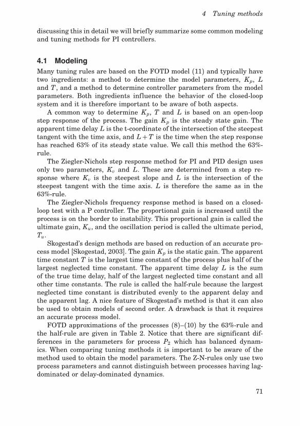
4 Tuning methods
discussing this in detail we will briefly summarize some common modelingand tuning methods for PI controllers.
4.1 Modeling
Many tuning rules are based on the FOTD model (11) and typically havetwo ingredients: a method to determine the model parameters, Kp, Land T , and a method to determine controller parameters from the modelparameters. Both ingredients influence the behavior of the closed-loopsystem and it is therefore important to be aware of both aspects.A common way to determine Kp, T and L is based on an open-loop
step response of the process. The gain Kp is the steady state gain. Theapparent time delay L is the t-coordinate of the intersection of the steepesttangent with the time axis, and L+T is the time when the step responsehas reached 63% of its steady state value. We call this method the 63%-rule.The Ziegler-Nichols step response method for PI and PID design uses
only two parameters, Kv and L. These are determined from a step re-sponse where Kv is the steepest slope and L is the intersection of thesteepest tangent with the time axis. L is therefore the same as in the63%-rule.The Ziegler-Nichols frequency response method is based on a closed-
loop test with a P controller. The proportional gain is increased until theprocess is on the border to instability. This proportional gain is called theultimate gain, Ku, and the oscillation period is called the ultimate period,Tu.Skogestad’s design methods are based on reduction of an accurate pro-
cess model [Skogestad, 2003]. The gain Kp is the static gain. The apparenttime constant T is the largest time constant of the process plus half of thelargest neglected time constant. The apparent time delay L is the sumof the true time delay, half of the largest neglected time constant and allother time constants. The rule is called the half-rule because the largestneglected time constant is distributed evenly to the apparent delay andthe apparent lag. A nice feature of Skogestad’s method is that it can alsobe used to obtain models of second order. A drawback is that it requiresan accurate process model.FOTD approximations of the processes (8)–(10) by the 63%-rule and
the half-rule are given in Table 2. Notice that there are significant dif-ferences in the parameters for process P2 which has balanced dynam-ics. When comparing tuning methods it is important to be aware of themethod used to obtain the model parameters. The Z-N-rules only use twoprocess parameters and cannot distinguish between processes having lag-dominated or delay-dominated dynamics.
71

Paper I. Performance and robustness trade-offs in PID control
Table 2. Apparent time delay L, apparent time constant T and normal-ized time delay τ for the processes P1 (8), P2 (9) and P3 (10) obtained bythe 63%-rule and Skogestad’s half-rule (1/2).
P1 P2 P3
63% 1/2 63% 1/2 63% 1/2
L 0.075 0.061 1.42 2.50 1.014 1.025T 1.041 1.050 2.93 1.50 0.093 0.075τ 0.067 0.055 0.33 0.63 0.92 0.93
4.2 The Ziegler-Nichols methods
The Ziegler-Nichols methods are included only for historical reasons. Ro-bustness to process uncertainty and measurement noise were not consid-ered. The step response method give the controller parameters
kp =0.9KvL
, ki =0.3KvL2
, Ti = 3L. (12)
The frequency response method is tuned to give quarter amplitudedamping of load disturbance responses and is given by
kp = 0.4Ku, ki =0.5KuTu
, Ti = 0.8Tu. (13)
As we have seen in Fig. 1, the Ziegler-Nichols methods result in poorcontrol for all three processes P1, P2 and P3. We should revere the Ziegler-Nichols rules for the original ideas, but they are not useful for practicalPID tuning and there are better methods to teach in e.g. basic controlcourses.
4.3 Lambda tuning
Lambda tuning originated in early computer control [Dahlin, 1968;Higham, 1968], was rediscovered in connection with the development ofinternal model control [Rivera et al., 1986] and is today widely adopted inthe industry, see e.g. [Sell, 1995; Bialkowski, 1996]. Modeling is typicallybased on measured step responses and the 63%-rule is used to obtainan FOTD model. The desired closed-loop time constant Tcl is used as atuning parameter. In the original work by Dahlin, Tcl was called λ , whichexplains the name of the tuning method. This parameter admits a com-promise between performance and robustness. For PI control the tuningformulas are
kp =T
Kp(Tcl + L), ki =
1Kp(Tcl + L)
, Ti = T (14)
72

4 Tuning methods
The process time constant is canceled by the controller zero which givessluggish load disturbance responses for processes with lag-dominated dy-namics. There are several suggestions for choosing Tcl, some can be foundin [Sell, 1995; Bialkowski, 1996]. We will mark the original choices ofTcl = T , 2T or 3T in the trade-off plots, but the whole set of possible con-trollers will also be plotted as a line through these three choices. Tcl = Tcorresponds to aggressive tuning and Tcl = 3T to robust tuning.
4.4 Skogestad’s methods
Skogestad [Skogestad, 2003] introduced modifications of the Lambda tun-ing method called SIMC that improves performance especially for lag-dominant processes. The FOTD model is obtained by model reduction ofa high-order process model using the half-rule.SIMC is closely related to Lambda tuning. Unlike the original Lambda
tuning, however, the desired closed-loop time constant Tcl is chosen as afactor of the apparent time delay L. Skogestad recommends Tcl = L asthe primary choice which typically gives a sensitivity close to Mst = 1.6.Less aggressive tuning is obtained for larger values of Tcl such as 2L and3L. In the trade-off plots we will examine these three choices of Tcl. Theparameters in the tuning rules were obtained by fitting to controllers thatwere optimized both for input and output disturbances.The proportional gain is chosen as kp in (14) and the integral time as
Ti = min(T , 4(Tcl + L)). (15)
This choice avoids cancellation of a slow process pole by a controller zerowhen T > 4(Tcl + L).A modified method, here called SIMC+, was introduced in [Skogestad
and Grimholt, 2012] to improve performance for delay-dominated systemswhere the SIMC rule results in controllers with too low proportional gain.Proportional gain and integral time were instead chosen as
kp =T + L/3Kp(Tcl + L)
, Ti = min(T + L/3, 4(Tcl + L)). (16)
For delay-dominated and balanced systems, the integral gain is the sameas for SIMC, the proportional gain kp and integral time Ti are larger thanfor SIMC.
4.5 Constrained optimization - AMIGO
The MIGO tuning method presented in [Panagopoulos et al., 2002] mini-mizes IE subject to the robustness constraint Mst ≤ 1.4. AMIGO [Åströmand Hägglund, 2005] is a design method obtained by applying MIGO to
73

Paper I. Performance and robustness trade-offs in PID control
a large test batch of process models and using simple parameter fitting.The parameters of the model are determined by the 63%-rule. The AMIGOtuning rule is
kp =0.15Kp
+(
0.35− LT
(L + T)2) T
KpL
Ti = 0.35L +13LT2
T2 + 12LT + 7L2
(17)
5. Assessment of tuning methods
The trade-off plots will now be used to assess the tuning methods for PIcontrol described in Section 4. The processes P1 (8), P2 (9) and P3 (10) willbe used to represent processes with lag-dominated, balanced and delay-dominated dynamics, and we will consider controllers that minimize IAEfor unit step load disturbances at the process input. Figure 3 is similarto Fig. 1 but the scales are different to show the parameter ranges ofinterest for tuning more clearly. The parameters corresponding to thedifferent tuning rules are shown in the diagram.The Ziegler-Nichols rules fall outside the plots except for the process
with delay-dominated dynamics in the case of the step response method,see Fig. 1. Both Lambda tuning, marked λ , and the SIMC rules, markedS and S+ respectively, use the tuning parameter, Tcl. These rules arerepresented by lines with marks for the choices of the design parametergiven in Sections 4.3 and 4.4. The AMIGO rule is marked with a bluecross and the letter A. The black line marked with triangles show thefollowing approximation
ki =kp + 0.1Kpk2p0.3L + 0.7T (18)
of the optimal, dash-dotted line. The approximation is valid for sensi-tivities Mst ≤ 1.6 and the model parameters L and T are given by the63%-rule.
5.1 Lag-dominated dynamics
The trade-off plot for the system P1 with lag-dominated dynamics is shownin the top plot of Fig. 3. Lambda tuning, with Tcl = T , 2T , 3T gives closed-loop systems with very low gains. The sensitivities are all less than 1.1,but the performance is poor because the gains are much too low. Lowervalues on Tcl give better performance, but it is still poor compared tothe optimal controllers. Comparing the set of controllers obtainable usingLambda tuning with the output disturbance optimal curve in Fig. 2, how-ever, shows that they are almost identical. Both SIMC rules give similar
74

5 Assessment of tuning methods
1.21.3
1.41.5
1.6
1.71.8
1.9
2
0 2 4 6 8 100
2
4
6
8
10
12
14
16
18
20
kp
ki
S
S
S
S+
S+
S+
A
λ
P1 - Lag-dominant dynamics
1.11.2
1.3
1.4
1.5
1.6
1.7
1.8
1.9
2
2.5
3
0 0.2 0.4 0.6 0.8 1 1.20
0.05
0.1
0.15
0.2
0.25
0.3
0.35
0.4
kp
ki S
SS
S+
S+
S+
A
λ
λ
λ
P2 - Balanced dynamics
1.2
1.3
1.4
1.5
1.6
1.7 1.8
1.9
2
0 0.05 0.1 0.15 0.2 0.25 0.3 0.35 0.40
0.1
0.2
0.3
0.4
0.5
0.6
0.7
0.8
0.9
1
kp
ki S
SS
S+
S+
S+
A
λλλ
Z-N
P3 - Delay-dominant dynamics
Figure 3. Trade-off plots for PI control of the processes P1, P2 and P3with controller parameters obtained with the tuning methods: Lambdatuning (λ), SIMC (S), modified SIMC (S+) and AMIGO (A). IAE-valuesare equal to 1/ki in the region where the levels are horizontal. The blacklines, marked by triangles, show a parametrization of the dash-dotted linesfor reasonable robustness given by (18).
75

Paper I. Performance and robustness trade-offs in PID control
performance with the choices Tcl = L, 2L and 3L. The sensitivity for thenominal design is Mst = 1.7 which is close to the design value 1.6. Thecontroller gains are generally higher than the constrained IAE-optimalcontrollers. The AMIGO method provides a controller which is close to itsdesign value Mst = 1.4.
5.2 Balanced dynamics
The trade-off plot for the system P2 with balanced dynamics is shown inthe center plot of Fig. 3. Lambda tuning gives closed-loop systems withgood performance and robustness, but the proportional gains are a littletoo high compared to the optimal controllers. SIMC gives good controllers,but the proportional gains are a little too low. SIMC+ gives close to opti-mal performance, but the sensitivities are lower than the design values.Notice, however, that by using SIMC and SIMC+ on the FOTD modelderived using the 63%-rule, with Tcl = L, the resulting controllers wouldhave the gains kp = 1.04, ki = 0.36 and kp = 1.20, ki = 0.36 respectively.Both controllers give poor closed-loop robustness with Mst > 2, showinghow important it is to use the recommended modeling procedure togetherwith the design method. AMIGO tuning gives a controller close to that ofthe Lambda tuning with a robustness slightly higher than the designedvalue.
5.3 Delay-dominated dynamics
The trade-off plot for the system P3 with delay-dominated dynamics isshown in the bottom plot of Fig. 3. The original Lambda tuning choices ofTcl = T , 2T and 3T give closed-loop systems with very poor robustness.The sensitivities are all larger than 2. Choosing a smaller value of Tclgives better robustness, but the proportional gains are still too low andthe integral gains too high compared with the optimal controllers. TheSIMC rule gives robustness that agrees well with the design value, butthe proportional gains are much too low. SIMC+ have the same integralgains, but larger proportional gains than SIMC. The performance is closeto optimal while the sensitivity for the case Tcl = L is slightly lower thanthe design value. The AMIGO rule gives a controller close to optimal withMst = 1.46, to compare with the design value 1.4.
5.4 Parametrization of optimal controllers
The green line that corresponds to optimal tuning is close to a straightline through the origin for balanced and delay-dominated systems andit is slightly curved for systems with lag-dominated dynamics. Choos-ing a Ti that corresponds to that line is a convenient way of describinghow performance and robustness varies simply by changing the gain. The
76
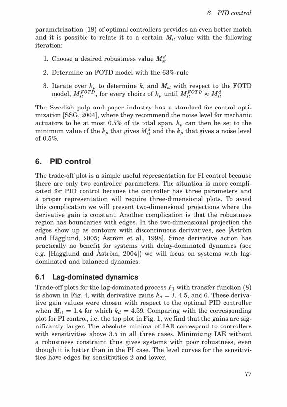
6 PID control
parametrization (18) of optimal controllers provides an even better matchand it is possible to relate it to a certain Mst-value with the followingiteration:
1. Choose a desired robustness value Mdst
2. Determine an FOTD model with the 63%-rule
3. Iterate over kp to determine ki and Mst with respect to the FOTDmodel, M FOTDst , for every choice of kp until M FOTDst ( Mdst
The Swedish pulp and paper industry has a standard for control opti-mization [SSG, 2004], where they recommend the noise level for mechanicactuators to be at most 0.5% of its total span. kp can then be set to theminimum value of the kp that gives Mdst and the kp that gives a noise levelof 0.5%.
6. PID control
The trade-off plot is a simple useful representation for PI control becausethere are only two controller parameters. The situation is more compli-cated for PID control because the controller has three parameters anda proper representation will require three-dimensional plots. To avoidthis complication we will present two-dimensional projections where thederivative gain is constant. Another complication is that the robustnessregion has boundaries with edges. In the two-dimensional projection theedges show up as contours with discontinuous derivatives, see [Åströmand Hägglund, 2005; Åström et al., 1998]. Since derivative action haspractically no benefit for systems with delay-dominated dynamics (seee.g. [Hägglund and Åström, 2004]) we will focus on systems with lag-dominated and balanced dynamics.
6.1 Lag-dominated dynamics
Trade-off plots for the lag-dominated process P1 with transfer function (8)is shown in Fig. 4, with derivative gains kd = 3, 4.5, and 6. These deriva-tive gain values were chosen with respect to the optimal PID controllerwhen Mst = 1.4 for which kd = 4.59. Comparing with the correspondingplot for PI control, i.e. the top plot in Fig. 1, we find that the gains are sig-nificantly larger. The absolute minima of IAE correspond to controllerswith sensitivities above 3.5 in all three cases. Minimizing IAE withouta robustness constraint thus gives systems with poor robustness, eventhough it is better than in the PI case. The level curves for the sensitivi-ties have edges for sensitivities 2 and lower.
77

Paper I. Performance and robustness trade-offs in PID control
1.41.5
1.6
1.7
1.8
1.9
22.5
2.5
3
3
33.5
3.5
3.5
44
4
4
0 50 100 150 200 250 300 350 4000
500
1000
1500
2000
2500
3000
3500
4000
4500
5000
kp
ki
P1 - Lag-dominant dynamics with kd = 6
1.3
1.3 1.41.5
1.6
1.7
1.8
1.9
2
2.5
3
3
33.5
3.5
3.5
4
4
4
0 50 100 150 200 250 3000
500
1000
1500
2000
2500
3000
kp
ki
P1 - Lag-dominant dynamics with kd = 4.5
1.21.4
1.61.8
2
2.5
3
3
4
4
4
55
5
5
0 50 100 150 200 2500
200
400
600
800
1000
1200
1400
1600
1800
2000
kp
ki
P1 - Lag-dominant dynamics with kd = 3
Figure 4. Trade-off plots for PID control of the process P1(s) = 1/((s+1)(0.1s + 1)(0.01s + 1)(0.001s + 1)), and derivative gains kd = 3 (lowergraph), kd = 4.5 (middle graph), and kd = 6 (top graph). The dash-dottedlines are the loci of controller gains that minimize IAE for a given ro-bustness. IAE-values are equal to 1/ki in the region where the levels arehorizontal.
78

6 PID control
If we require that the maximum sensitivity is Mst = 1.4, Fig. 4 showsthat the controllers with kd = 3, 4.5 and 6 have the IAE values 0.0021,0.0013, and 0.0016. The constrained minimum is IAE = 0.0013 for kp =89.48, ki = 1037.5, and kd = 4.59. The IAE value can be compared withthe corresponding value for PI control IAE = 0.1175. Adding derivativeaction thus improves performance by a factor 90. Since the gains are largeit is important to consider the effect of measurement noise and it maytherefore be essential to either impose constraints on the proportionaland derivative gains or add a noise filter. The dash-dotted lines in thetrade-off plots give guidance for detuning.
6.2 Balanced dynamics
Fig. 5 presents trade-off plots for the process P2 with derivative gainskd = 1, 2, and 3. The derivative gains were chosen with respect to theoptimal PID controller when Mst = 1.4 for which kd = 1.78. Comparingwith the corresponding plot for PI control, the center plot in Fig. 1, wefind that the plots are similar. The gains are larger with derivative ac-tion and the sensitivity curves have peaks with discontinuous derivatives.The absolute minima of IAE without robustness constraint correspond tocontrollers with poor robustness, the sensitivities are close to 2.5 in allthree cases. If we require that the sensitivities are less than 1.4, Fig. 5shows that the controllers with kd = 1, 2 and 3 have the IAE values 2.5,2.2 and 3.5. The constrained minimum for Mst = 1.4 is IAE = 2.14 forkp = 1.33, ki = 0.63, and kd = 1.78. The IAE value can be comparedwith the corresponding value for PI control, IAE = 4.4, adding derivativeactions thus improves performance by a factor 2.Figure 5 also shows that minimization of IE and IAE do not give the
same controllers except if the robustness constraint requires very lowsensitivity. The dash-dotted line which corresponds to the constrainedminimum has a plateau for large values of kd, giving it quite a differentshape than for PI control. Notice that the dash-dotted line is close tothe robustness constraint levels for small values of the sensitivities. Thismeans that the performance can be improved quite a bit almost withoutcosting anything in terms of robustness. This was also the case for processP1 in Fig. 4.
6.3 Measurement noise filtering
One reason why derivative action is not so commonly used in processindustry is that undesired valve motions are created by measurementnoise. The effect can be reduced by filtering the measurement signal, butgood rules for finding the filter time constant are missing. As pointed
79
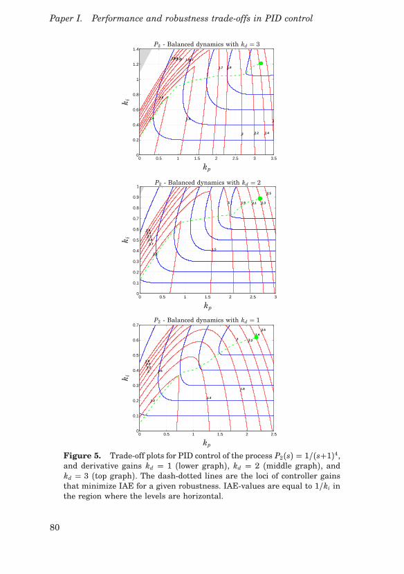
Paper I. Performance and robustness trade-offs in PID control
1.4 1.5
1.6
1.7
1.7
1.8
1.8
2
2
2.2
2.2
2.4
2.4
2.6
2.6
0 0.5 1 1.5 2 2.5 3 3.50
0.2
0.4
0.6
0.8
1
1.2
1.4
kp
ki
P2 - Balanced dynamics with kd = 3
1.3
1.5
1.7
1.7
1.9
1.9
2.1
2.1
2.3
2.3
2.5
2.5
0 0.5 1 1.5 2 2.5 30
0.1
0.2
0.3
0.4
0.5
0.6
0.7
0.8
0.9
1
kp
ki
P2 - Balanced dynamics with kd = 2
1.21.4
1.6
1.8
2
2
2.2
2.2
2.4
2.4
2.6
2.6
0 0.5 1 1.5 2 2.50
0.1
0.2
0.3
0.4
0.5
0.6
0.7
kp
ki
P2 - Balanced dynamics with kd = 1
Figure 5. Trade-off plots for PID control of the process P2(s) = 1/(s+1)4,and derivative gains kd = 1 (lower graph), kd = 2 (middle graph), andkd = 3 (top graph). The dash-dotted lines are the loci of controller gainsthat minimize IAE for a given robustness. IAE-values are equal to 1/ki inthe region where the levels are horizontal.
80

7 Conclusions
out by Isaksson and Graebe [Isaksson and Graebe, 2002], the filter timeconstant should be included in the control design.To illustrate the effect of measurement noise, we consider the balanced
process, P2, with discrete-time white Gaussian measurement noise withstandard deviation σ n = 1% and a sampling time of 0.01 seconds. ThePID controller designed for Mst = 1.4 in Section 6.2 has the parameterskp = 1.33, ki = 0.63 and kd = 1.78. Using a first-order filter on thederivative part with filter time constant T f = Td/N, and the commonchoice N = 10, we get T f = 0.13. A Matlab Simulink simulation givesthe standard deviation of the control signal σu = 14.4%. The maximumsensitivity increase to Mst = 1.52 from 1.4 because of the added dynamics,at the same time as the IAE-value for an input disturbance improves toIAE = 2.07 from 2.14. A greater N-value would give better noise filtering,but at the same time also give worse robustness.Garpinger’s PID tuning method in [Garpinger, 2009] can deal with
filtering and at the same keep the robustness constraints satisfied. As-suming that we want to decrease the variation in the control signal fromσu = 14.4% to σu = 0.5%, as suggested in Section 5.4, we can proceedas follows. Introduce a second order measurement filter with fixed filterdynamics and perform the controller optimization. Then iterate on T f un-til the standard deviation of the control signal satisfies the constraints.Using this procedure, we find that T f = 0.38, kp = 0.91, ki = 0.40 andkd = 1.22, with IAE = 3.18, fulfill both the robustness and the noisecriteria. The trade-off plot with kd = 1.22 and T f = 0.38 is shown inFig. 6. As one could expect, the controller gains are lower than withoutfiltering, however, the level curves look similar to those without filtering.Notice that T f is significantly larger than the value obtained by the ruleof thumb N = 10. The IAE-value is 49% higher than with the unfilteredcontroller. The best PI controller has IAE = 5.2, 63% higher than thefiltered PID controller, and σu = 0.43%. This shows that there is a lot togain from using derivative action, even when measurement noise is takencare of.
7. Conclusions
A graphical tool which provides insight into the trade-offs between perfor-mance and robustness for PID control has been introduced. The trade-offis represented by charts which show the level curves of performance, ex-pressed by integrated absolute error (IAE), and robustness, expressed bythe maximum sensitivity (Mst), as functions of proportional and integralgain. For PID control the charts are drawn for fixed values of the deriva-tive gain. The trade-off charts are useful to provide intuition about tuning,
81

Paper I. Performance and robustness trade-offs in PID control
1.3
1.3
1.4
1.5
1.6
1.7
1.8
1.9
1.9
2
2
2.1
2.1
2.2
2.2
0 0.5 1 1.5 20
0.1
0.2
0.3
0.4
0.5
0.6
kp
ki
P2 - Balanced dynamics with kd = 1.22, T f = 0.38
Figure 6. Trade-off plot for PID control of the balanced process P2(s) =1/(s+1)4, with derivative gain kd = 1.22 and low-pass filter time constantT f = 0.38. IAE-values are equal to 1/ki in the region where the levels arehorizontal.
both for practitioners and students. They can also show the difference be-tween tuning criteria based on input and output disturbances.The level curves of performance are practically horizontal in large ar-
eas of the plots, which indicate that the integral gain is directly relatedto performance and the proportional gain directly related to robustness.These areas have interesting properties: IAE is a monotone function ofki and close to IE, Mst is a function of kp with a maximum for each ro-bustness value. For fixed integral time, controllers are represented bystraight lines in the plots, and adjustments of the proportional gain theninfluence both robustness and performance. This fact can be used empir-ically by exploring a few values of the proportional gain. There is also aparametrization of controllers (18) that corresponds to optimal tuning forinput disturbances, which can be related to a certain robustness throughiteration over kp.In process control it has been a tradition to separate processes with
and without integral action. A more graduated separation can be obtainedby introducing the normalized time delay τ , which is in the range 0 to1. For an FOTD model we have τ = L/(L + T). Analysis of the trade-off charts shows that there is a significant difference between processeswith lag-dominant (τ ≤ 0.2), balanced 0.2 < τ < 0.7, or delay-dominant(τ ≥ 0.7) dynamics. By obtaining an FOTD model e.g. with the 63%-rule
82

References
one can then calculate τ and choose a corresponding plot to analyze. Thebenefit of derivative action is marginal for processes with delay-dominateddynamics but significant for processes with lag-dominated dynamics. Theproportional gain is typically high for processes with lag-dominated dy-namics indicating the necessity to take measurement noise into accounteven with PI control. With PID control the proportional gains are higheven for processes with balanced dynamics indicating the necessity of fil-tering the measured signal. The trade-off plot with filtering is similar tothe unfiltered case, but the gains are smaller.The trade-off plots were used to compare different tuning methods
for PI control. For input disturbances, Lambda tuning only gives good re-sults for processes with balanced dynamics, although it is close to optimalfor output disturbances on lag-dominant processes. The weakness of theLambda method lies in the choice Ti = T , which gives a set of controllerswith the slope 1/T . As the plots indicate, this slope deviates significantlyfrom the set of optimal controllers. For delay-dominant processes, Lambdatuning will either give poor robustness or poor performance, dependingon the choice of Tcl. SIMC gives decent results for at least lag-dominantand balanced processes. SIMC+ is a real improvement since it gives closeto optimal tuning also for systems with delay-dominated dynamics. BothSIMC methods depend on having an accurate process model which is re-duced using Skogestad’s half-rule. The predicted sensitivity of Mst = 1.6for Skogestad’s rules with Tcl = L is close to the truth. The AMIGOmethod is based on FOTD models, where the parameters are determinedusing the step response method. It gives controllers with sensitivity closeto the specified value Mst = 1.4.
Acknowledgements
This work was partly funded by the Swedish Foundation for Strategic Re-search through the PICLU center. The authors are members of the LCCCLinnaeus Center and the ELLIIT Excellence Center at Lund University.
References
Alcántara, S., R. Vilanova, and C. Pedret (2013). “PID control in termsof robustness/performance and servo/regulator trade-offs: A unifyingapproach to balanced autotuning”. Journal of Process Control 23:4,pp. 527–542.
Åström, K. J. and T. Hägglund (2005). Advanced PID Control. ISA – TheInstrumentation, Systems, and Automation Society, Research TrianglePark, NC.
83

Paper I. Performance and robustness trade-offs in PID control
Åström, K. J., H. Panagopoulos, and T. Hägglund (1998). “Design ofPI Controllers based on Non-Convex Optimization”. Automatica 34:5,pp. 585–601.
Bialkowski, W. L. (1996). “Control of the Pulp and Paper Making Process”.In: Levine, W. S. (Ed.). The Control Handbook. CRC Press, Inc, BocaRaton, Florida. Chap. 72, pp. 1219–1242.
Dahlin, E. B. (1968). “Designing and tuning digital controllers”. Instru-ments and Control Systems 41:6, pp. 77–83.
Franklin, G. F., J. D. Powell, and A. Emami-Naeini (2010). Feedback Con-trol of Dynamic Systems. 6th Edition. Pearson, Upper Saddle River,NJ.
Garpinger, O. (2009). Design of Robust PID Controllers with ConstrainedControl Signal Activity. Licentiate Thesis ISRN LUTFD2/TFRT--3245--SE. Department of Automatic Control, Lund University, Swe-den.
Hägglund, T. and K. J. Åström (2004). “Revisiting the Ziegler-Nichols stepresponse method for PID control”. Journal of Process Control 14:6,pp. 635–650.
Higham, J. D. (1968). “‘Single-term’ control of first- and second-orderprocesses with dead time”. Control 12, pp. 136–140.
Isaksson, A. and S. Graebe (2002). “Derivative filter is an integral part ofPID design”. Control Theory and Applications, IEE Proceedings 149:1,pp. 41–45.
Kristiansson, B. and B. Lennartson (2006). “Evaluation and simple tuningof PID controllers with high-frequency robustness”. Journal of ProcessControl 16 (2), pp. 91–102.
Larsson, P.-O. and T. Hägglund (2011). “Control Signal Constraints andFilter Order Selection for PI and PID Controllers”. In: 2011 AmericanControl Conference. San Francisco, California, USA.
Marlin, T. (1995). Process Control – Designing Processes and Control Sys-tems for Dynamic Performance. Chemical Engineering. McGraw-Hill,New York, USA.
McMillan, G. (1983). Tuning and Control Loop Performance. ISA, Re-search Triangle Park, NC.
Panagopoulos, H., K. J. Åström, and T. Hägglund (2002). “Design of PIDcontrollers based on constrained optimisation”. IEE Proceedings - Con-trol Theory & Applications 149:1, pp. 32–40.
Rivera, D. E., M. Morari, and S. Skogestad (1986). “Internal Model Con-trol. 4. PID Controller Design”. Ind. Eng. Chem. Process Des. Dev. 25,pp. 252–265.
84

References
Romero Segovia, V., T. Hägglund, and K. J. Åström (2013). “Noise fil-tering in PI and PID Control”. In: 2013 American Control Conference.Washington, D.C., USA.
Sell, N. J., (Ed.) (1995). Process Control Fundamentals for the Pulp &Paper Industry. Tappi Press, Technology Park, Atlanta, GA.
Shinskey, F. G. (1996). Process-Control Systems. Application, Design, andTuning. 4th. McGraw-Hill, New York, NY.
Skogestad, S. (2003). “Simple analytic rules for model reduction and PIDcontroller tuning”. Journal of Process Control 13:4, pp. 291–309.
Skogestad, S. and C. Grimholt (2012). “The SIMC Method for Smooth PIDController Tuning”. In: Vilanova, R. et al. (Eds.). PID Control in theThird Millenium. Springer-Verlag, London. Chap. 5, pp. 147–175.
SSG (2004). Regleroptimering (in Swedish). 3rd. SSG 5253.
85


Paper II
A software tool for robust PIDdesign
Olof Garpinger Tore Hägglund
Abstract
This paper presents a fast, interactive and easily modifiable softwaretool for robust PID design. The MATLAB®-based program is supposedto give people with moderate knowledge on PID control a possibility tolearn more and also be a future part of an autotuner. The PID designis made by minimizing the integrated absolute error value during aload disturbance on the process input. The optimization is performedwith H∞-constraints on the sensitivity and complementary sensitiv-ity function, providing a robust closed-loop system. Nelder-Mead op-timization is used with the AMIGO method providing an initial con-troller. The proposed method works well, and is very efficient, on alarge batch of systems common in process industry. The design toolis also shown to work on a highly oscillatory process model.
©2008 IFAC. Reprinted, with permission, from Proceedings of the 17thIFAC World Congress, Seoul, South Korea, 2008.
87

Paper II. A software tool for robust PID design
1. Introduction
The PID controller is by far the most common controller in industry today.Even so, a lot of these controllers are poorly tuned. Two of the mainreasons for that is lack of knowledge and time among the operators. Asa consequence, many controllers are set to default values. In other cases,the derivative part is turned off because it was not used correctly, givingnoisy signals. It would therefore be a good idea to educate the operators inthe possibilities of the PID controller and to provide them with simple andfast design tools. This paper describes a program that achieves both goalsand should be useful for people in the industry as well as for academics.There are many PID design methods available today and some of the
most famous are collected and analysed in [Åström and Hägglund, 2005].Of these, the MIGO and AMIGO methods (also see [Panagopoulos et al.,2002] and [Hägglund and Åström, 2004]) are probably those most worthmentioning in connection to this paper. They are based on optimization ofload disturbance rejection under robustness constraints. A further devel-opment of the MIGO method, and largely based on the same method asused in this paper, was presented in [Nordfeldt, 2005]. An advantage withNordfeldt’s method is that it also works for some more advanced processstructures. This paper focuses on the software that solves the optimiza-tion problem and how it can be used to increase people’s understandingof PID control.The proposed PID control design method is incorporated in several
MATLAB® functions. There are many good reasons to have a softwarebased tool for control design and analysis. In [Åström and Hägglund, 2001]it is pointed out that it would be of great value to have software that cangive persons with moderate knowledge on PID controllers a possibility toexperiment on those and at the same time be able to use the program tobuild controllers for a real plant, by incorporating it into an autotuningprocedure. For simulation experiments and real use purposes, the pre-sented software is able to provide a well working controller with analysistools in just a few seconds time. The advanced user should also be ableto modify the optimization problem to broaden the possibilities. Besidesthe proposed program, which is intended to be free of charge and down-loadable, there are already several commercial software packages able toprovide PID design tools using a variety of methods. Many of these arecollected in [Li et al., 2006] and another one with very similar features tothe proposed is presented in [Oviedo et al., 2006].
88

2 Design criterion
C(s) P (s)
−1
d
yue
n
ΣΣ
Figure 1. A load disturbance, d, and measurement noise, n, act on theclosed-loop system with process P(s) and PID controller C(s).
2. Design criterion
The proposed PID controller design tool is mainly meant to work wellfor systems common in process industry. The kind of plants encounteredthere are often stable, monotone and primarily affected by low frequencyload disturbances.In order for the controller design to work well on a process, P(s), it
is important to take all system signals into consideration, especially ifoptimization is used. Figure 1 shows a block diagram of the system thatthe PID controller, C(s), is designed for. There are two external signalsentering the system, namely load disturbance d (mainly low frequency)and measurement noise n (assumed high frequency). Of the closed-looptransfer functions, those of greatest interest for this paper are the com-plementary sensitivity function T(s) and the sensitivity function S(s),defined as
T(s) = P(s)C(s)1+ P(s)C(s) , S(s) =
11+ P(s)C(s) .
The PID controller is on parallel form with a second order low pass filter
C(s) = K(
1+ 1sTi
+ sTd)
⋅1
1+ sT f + (sT f )2/2,
on the measurement signal. T f , is chosen to weight the degree of mea-surement noise rejection.The objective of the proposed PID design method is to find the PID
controller giving the least integrated absolute error (IAE) value when aload disturbance d, modelled as a step, is acting on the closed-loop system.
89

Paper II. A software tool for robust PID design
The optimization is done under the constraints that the closed-loop systemis stable and that the open loop Nyquist curve is tangent to one or twoprespecified circles in the complex plane without entering either of them(see Fig. 2), thus maximizing the gain. These two circles are called theMs- and Mt-circles, which sizes and positions are given by
Ms = maxωpS(iω )p, Mt = max
ωpT(iω )p,
hence the names. The resulting, non-convex, optimization problem can bewritten as
minK ,Ti,Td∈R+
∞∫
0
pe(t)pdt = IAEload (1)
subject to pGo(iω ) − CMs p2 ≥ R2Ms ∀ω ∈ R+,
pGo(iω ) − CMt p2 ≥ R2Mt ∀ω ∈ R+,
pGo(iω s) − CMs p2 = R2Ms ,pGo(iω p) − CMt p2 = R2Mt ,
where e(t) is the control error, Go(iω ) is the open-loop frequency response,ω s are frequencies for which Go(iω ) is tangent to the Ms-circle and viceversa for ω p on the Mt-circle. Either ω s or ω p could be an empty vector,but not at the same time. The radius and centre point of the Ms-circleare denoted by RMs and CMs respectively, with corresponding measuresfor the Mt-circle, RMt and CMt . Small Ms- and Mt-values result in largecircles. In the software, the maximum allowed Ms- and Mt-values can beprespecified by the user (Ms = Mt = 1.4 is default, resulting in 41.8○ phasemargin). The Ms- and Mt- criterions are known to set the closed-looprobustness towards process variations, disturbances and nonlinearitiesas described in [Åström and Hägglund, 2005]. MIGO on the other handuses a simplified robustness criterion called the M -circle, defined as thesmallest circle that can be drawn around both the Ms- and Mt-circle.
3. Algorithm overview
The main goal of the new design algorithm was to develop a fast, inter-active and easily modifiable software tool for robust PID design.A non-convex optimization problem like (1) may have many local min-
ima. It is therefore hard to guarantee that the solution obtained always isthe global solution. It is also difficult to draw any general analytical con-clusions as the problem is far from trivial. The method of gridding does
90

3 Algorithm overview
-4 -3 -2 -1 0 1-2
-1.5
-1
-0.5
0
0.5
1
1.5
2
Real axis
Imag
inar
y ax
is
Figure 2. The Ms-circle (dashed), Mt-circle (dash-dotted) and the open-loop Nyquist curve (solid) when the optimization criterions are fulfilled.
however give a possibility of drawing surface plots of the cost function.These can be used to determine whether or not it is likely that a givensolution is in fact the global minimum. This is also the major reason whygridding is an optional optimization method in the proposed design pro-gram.Analysis of many cost function surfaces have shown that if not all,
then at least a lot of them only have one minimum. This finding gave theidea to use a faster and more advanced optimization tool than gridding,called the Nelder-Mead (NM) method, [Nelder and Mead, 1965], in orderto find the minimum in the Ti-Td plane, see below.The new algorithm can be summarized by
1. Given a linear transfer function, initial PID parameters are chosenusing the AMIGO method.
2. NM optimization finds the PID controller giving the minimum costfunction in the Ti-Td plane.
91

Paper II. A software tool for robust PID design
a) For each Ti-Td couple, a proportional gain, K , is found suchthat the constraints are fulfilled.
b) Simulink® simulations are used to calculate IAE-values in thepoints through which the NM method proceeds.
An interactive program menu has been added to make it possible forthe user to change a number of settings in the algorithm as well as forthe presentation of the results. When the program is run in MATLAB®,the menu will come up unless the opposite is stated by the user. Newdefault values for the optimization can also be set as input parameter.This is especially useful for batch runs, when you may want to choose thesettings before a number of program runs are started. An experienceduser should easily be able to modify the program, to for instance, changethe optimization method or at least to change the cost function.
4. Algorithm details
In this section, the optimization algorithm will be explained in furtherdetail.
4.1 The Nelder-Mead method
Nelder-Mead optimization belongs to the subclass of optimization methodscalled direct search methods. The main theme among these is that theyonly use function values without creating approximations of the functiongradients explicitly. These methods are especially useful if, for instance,the cost to evaluate the function is high and if it is impossible to derive theexact gradient. These statements apply to the optimization problem (1).Whenever the cost function is evaluated, the feasible proportional gainsmust be calculated and Simulink® simulations run. The simulations areparticularly costly if the given PID parameters, at a certain grid point,gives a very sluggish closed loop.The Nelder-Mead method is a simplex-based method. There are many
papers and books which describe in detail how the NM algorithm works(see for instance [Walters et al., 1991] and [Lagarias et al., 1998]). Two ofthe reasons why the method is popular are that it is easy to both under-stand and implement. It is only necessary to look at two dimensional NMoptimization in this paper as (1) can be viewed as an unconstrained min-imization problem in R
2, when K is chosen separately. Two dimensionalNM optimization can be interpreted as triangle search progression withvariable area. In order to begin the NM optimization, an initial trianglehas to be specified. The function to be minimized - lets call it f - is eval-uated at all three edges and the points are sorted in the order: B (best,
92

4 Algorithm details
1.5 2 2.5 3 3.5 4 4.5-0.5
0
0.5
1
1.5
2
2.5
3
3.5
W
B G
M
C1
C2
R
E
S
Figure 3. The Nelder-Mead progression in one iteration. The initial sim-plex is the one with corners in B, G and W. The simplex will change it’sshape depending on function evaluations in closely situated points.
lowest function value f (B)), W (worst, highest function value f (W)) andG (good, function value, f (G), in between the other two). From this point,the algorithm will alter the shape of the triangle to give a new one withless total cost. These steps are well explained in the given sources andwill not be presented in further detail here. Figure 3 gives a hint of pos-sible new simplexes. When a new simplex has been determined - againwith corners B, G and W - the algorithm will iterate until a terminationcondition has been fulfilled.
4.2 Initial values
It is preferable to have a good initial guess of where the minimum islocated to have fast convergence of the optimization. Another reason isthat there is a chance - although not so big when solving (1) - of endingup in a local minimum. The method used to receive an initial controllerin the proposed algorithm is called AMIGO, which is a tool for robustPID (and PI) synthesis. To understand AMIGO, it is also important tounderstand the MIGO method for PID design.The optimization problem that the MIGO design deals with is very
93

Paper II. A software tool for robust PID design
similar to (1). But instead of minimizing over the IAE-value, it uses theIntegrated Error,
IEload =∞∫
0
e(t)dt,
as cost function and the M -circle as robustness constraint, to determinethe PID parameters. The IE cost is proportional to 1/ki = Ti/K , whichreduces the problem to maximizing the ki-gain over the robustness area.The AMIGO design is basically a set of formulas yielding K , Ti and
Td. In order to determine these, the MIGO method was run on a largenumber of systems common in process industry (with Ms = Mt = 1.4).Secondly, each and every process in the batch was approximated as afirst-order system with time delay (FOTD)
Gp(s) =Kp
sT + 1 e−sL. (2)
The PID-parameters were then plotted versus the normalized time de-lay, τ = L/(L + T), and parameter fittings were made on these curvesresulting in the formulas.In the proposed PID design method, the system of interest is approx-
imated as a FOTD system, (2), through a step response test and theAMIGO parameters are then determined. Let the index A denote theAMIGO PID parameters. The AMIGO parameters provided are used asone of the corners, (T Ad ,T Ai ), in the initial Nelder-Mead simplex. Takinginto account that the evaluation time is usually greater far out in theTi-Td plane, the two remaining corners have been set to (0.4T Ad ,T Ai ) and(T Ad , 0.4T Ai ).
4.3 Determining the proportional gain K
The key idea to find K in every point (Td,Ti), is to determine all K -valuesputting the open-loop Nyquist curve on a circle in the complex plane (atevery frequency point ω ), resulting in a function K (ω ). Since the methodis numerical, the frequency span is divided into a finite number of pointsω k, k = 1, 2, .... In order to determine K (ω ), let us first assume that theopen-loop frequency response, Go(iω ), can be written as
Go(iω ) = K (X (ω ) + iY(ω )), (3)
where X (ω ) and Y(ω ) are the real and imaginary parts of G′o(iω ) =Go(iω )/K . From the optimization problem (1) we have the constraint
pGo(iω ) − Cp2 = R2, (4)
94

4 Algorithm details
for any circle with center in C and radius R. Using (3) and (4), butchanging K to K (ω ), will lead to
(K (ω )X (ω ) − C)2 + (K (ω )Y(ω ))2 = R2 [
K (ω )2 − 2CX (ω )X (ω )2 + Y(ω )2 K (ω ) +
C2 − R2X (ω )2 + Y(ω )2 = 0. (5)
The two solutions correspond to the gains for which the open-loop Nyquistcurve will cross the front and back side of the circle respectively (seeFig. 4)
K1,2(ω ) =CX (ω ) ±
√
R2(X (ω )2 + Y(ω )2) − C2Y(ω )2)X (ω )2 + Y(ω )2 . (6)
K1,2(ω ) could for instance look like the plots in Fig. 5. For some fre-quency points, (6) will assume imaginary or negative numbers, whichare discarded. In the intervals for which K assumes positive real values,there can be multiple minima and maxima.There are a few observations needed in order to conclude which K -
values will fulfill the constraints in (1).THEOREM 1The open-loop Nyquist curve, (3), of an arbitrary controlled process, willbe tangent to a circle in the complex plane, given by the center point Cand radius R, if and only if
dK1(ω )dω
= 0 or dK2(ω )dω
= 0 (7)
Proof In vector form, the open-loop frequency response becomes
Go(iω ) = K(
X (ω )Y(ω )
)
. (8)
There are two conditions that has to be fulfilled in order for the open-loop Nyquist curve to be tangent to the circle at a given frequency pointω ∗. The open-loop Nyquist curve should lie on the circle determined by
(K X (ω ∗) − C)2 + (KY(ω ∗))2 = R2, (9)
while the tangent of the open-loop Nyquist curve and the vector betweenthe center point and Nyquist curve should be orthogonal
(
dGo(iω ∗)dω
)T (K X (ω ∗) − CKY(ω ∗)
)
= 0. (10)
95

Paper II. A software tool for robust PID design
-4 -3.5 -3 -2.5 -2 -1.5 -1 -0.5 0 0.5-2
-1.5
-1
-0.5
0
0.5
1
1.5
2
Real Axis
Imag
inar
y A
xis
K1(iωk)
K2(iωk)
G′
o(iωk)
Figure 4. Proportional gain functions K1(ω k), K2(ω k), for whichK jG
′o(iω k), j ∈ [1, 2], is tangent to a circle in the complex plane. G ′o(iω k) is
the open-loop frequency response with K = 1 and ω k denotes the discretefrequency points.
Denoting X ′(ω ) = dX (ω )/dω , Y ′(ω ) = dY(ω )/dω , (10) can be rewrittenas
(
K X ′(ω ∗)KY ′(ω ∗)
)T (K X (ω ∗) − CKY(ω ∗)
)
=
K 2X (ω ∗)X ′(ω ∗) − KCX ′(ω ∗) + K 2Y(ω ∗)Y ′(ω ∗) = 0,
and in turn, by solving for K , we end up with
K = CX ′(ω ∗)X (ω ∗)X ′(ω ∗) + Y(ω ∗)Y ′(ω ∗) . (11)
Let us now go back to Eq. (5). Taking the derivative with respect to ω ,
96

4 Algorithm details
0.8 1 1.2 1.4 1.6 1.80
2
4
6
8
10
12
14
16
18
ω (rad/s)
Pro
port
iona
l gai
n K
Figure 5. A constructed sketch of how the functions K1(ω ) (solid) andK2(ω ) (dashed) could look for a time-delayed system. Only K -valuesunique in ω - i.e. the first two minima and first maximum in this case- will fulfill the circle constraints in (1).
given that K ′(ω ) = dK (ω )/dω , leaves us with
2KK ′X 2 + 2K 2X X ′ − 2CK ′X − 2CK X ′+2KK ′Y2 + 2K 2YY ′ = 0, (12)
with ω omitted. Using K ′(ω ) = 0, results in
K (ω )X (ω )X ′(ω ) − CX ′(ω ) + K (ω )Y(ω )Y ′(ω ) = 0[
K (ω ) = CX ′(ω )X (ω )X ′(ω ) + Y(ω )Y ′(ω ) , (13)
which is identical to (11) in ω ∗. Since (9) is fulfilled for all frequencies inK (ω ), the proof is concluded. ✷
Go(iω ) can, however, be tangent to the circle on both the inside oroutside, but still have points within (thus giving an infeasible solution).To explain why, it is a good idea to once again view Fig. 4. At a given fre-quency point ω k, it is obvious that all proportional gains between K1(ω k)
97

Paper II. A software tool for robust PID design
and K2(ω k) will place Go(iω ) inside the circle, thus resulting in infeasibleK . Looking at Fig. 5, this means that only the minima and maxima, forwhich K is unique in ω , are feasible. For this particular case, it corre-sponds to the first two minima and first maximum.Once all possible K -values have been determined (the two minima and
the maximum from Fig. 5 for example), closed-loop stability is evaluated.If there is stability, the optimal proportional gain at a given point in theTi-Td plane, is then given by the K resulting in the lowest IAE-value(determined by Simulink® simulations).Up to now it has been assumed that it is just one circle in the com-
plex plane that the open-loop Nyquist curve may be tangent to. Since theconstraints of (1) demands that the Nyquist curve is located outside boththe Ms- and Mt-circles, the algorithm has to be run twice.
5. Examples
In this section there will be a few examples highlighting the benefits ofthe proposed program and algorithm compared to other methods. It willalso show that the new method is reliable in many design cases.
EXAMPLE 1—THE AMIGO TEST BATCH
The AMIGO formulas, [Hägglund and Åström, 2004], were derived usingMIGO on a test batch, which includes 134 essentially monotone systemscommon in process industry.In order to compare with the MIGO PID designs on the batch, the PID
design software presented in this paper was modified to use the M -circleas constraint. It took the program just more than one hour to run throughall sub-batches except some integrating processes. This gives an averagetime of 30 seconds per process in the batch. The batch was however runto get a high accuracy on the optimal solution rather than optimized fora fast design. If speed is of essence, the average design time per processcould be cut by at least two thirds of the time. The designs was run onan Intel® Dual-Core™, 2.13 GHz with 1 GB RAM and Fedora™ 7 usingMATLAB® 7 R2007a. The only two parameters that had to be modifiedfrom the default values (depending on the process) in order for the batchto run through properly, were T f and the frequency grid.The PID parameters derived by the proposed algorithm were compared
to those given by the MIGO method. Since the MIGO method was notderived to minimize IAE, the proposed method should give lower valuesat all times. The MIGO method is however a good indicator to see if thenew algorithm works or not. The batch run showed that the two methodsare very similar. In average, the new controllers resulted in IAE values at
98

5 Examples
0 0.2 0.4 0.6 0.8 130
40
50
60
70
80
90
100
Normalized time delay τ
Per
cent
ual I
AE
diff
eren
ce (
%)
Figure 6. IAE values comparison for the testbatch using the M -circleconstraint alone or both the Ms- and Mt-circles. The plot displays 100 ⋅IAEMs ,Mt/IAEM as a function of τ .
95% of what the MIGO controllers gave over the whole batch. This givesboth a strong indicator that the new program works properly and that theMIGO method gives essentially IAE minimized controllers for the batch.To see the benefit of using the Ms- and Mt-circles instead of the M -
circle, the whole batch was compared when the two different constraintswere used respectively. Figure 6 shows that the biggest percentual gainis given for low values on the normalized time delay, τ , while more delaydominated systems are less dependent on the choice of the constraints.This indicates that the IAE can be decreased a great deal without chang-ing the essential robustness constraints.The one subbatch where the newly proposed PIDs gave IAE values
with the most deviation from the MIGO ones was
P(s) = 1(s+ 1)((sT)2 + 1.4sT + 1) , (14)
with T = 0.1, 0.2, 0.3, 0.4, 0.5, 0.6, 0.7, 0.8, 0.9, 1.0.,
i.e. processes with complex poles. In particular, when T = 0.1, the newIAE is as small as 62.5% of the MIGO IAE, corresponding to a significantimprovement. Figure 7 shows the output signal, y, and control signal, u,when a load disturbance, d (see Fig. 1), is acting on this process. The
99
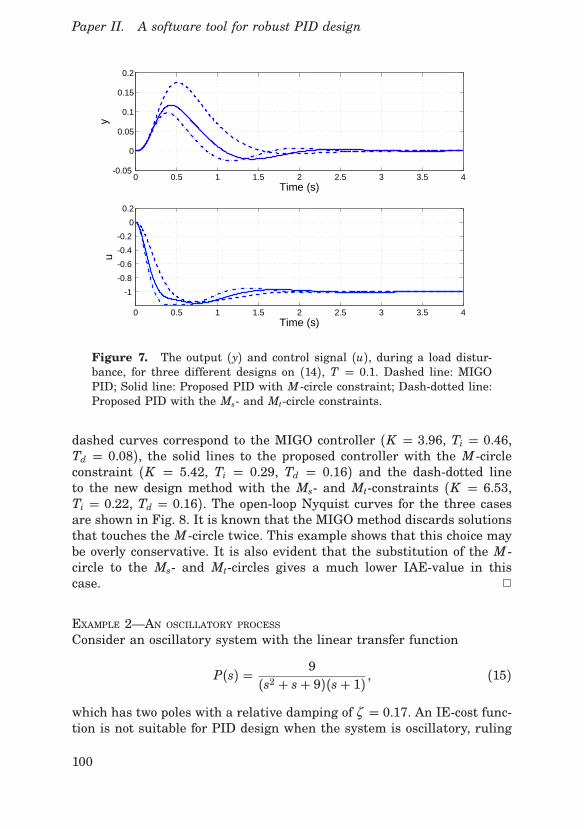
Paper II. A software tool for robust PID design
0 0.5 1 1.5 2 2.5 3 3.5 4
-1
-0.8
-0.6
-0.4
-0.2
0
0.2
Time (s)
u
0 0.5 1 1.5 2 2.5 3 3.5 4-0.05
0
0.05
0.1
0.15
0.2
Time (s)
y
Figure 7. The output (y) and control signal (u), during a load distur-bance, for three different designs on (14), T = 0.1. Dashed line: MIGOPID; Solid line: Proposed PID with M -circle constraint; Dash-dotted line:Proposed PID with the Ms- and Mt-circle constraints.
dashed curves correspond to the MIGO controller (K = 3.96, Ti = 0.46,Td = 0.08), the solid lines to the proposed controller with the M -circleconstraint (K = 5.42, Ti = 0.29, Td = 0.16) and the dash-dotted lineto the new design method with the Ms- and Mt-constraints (K = 6.53,Ti = 0.22, Td = 0.16). The open-loop Nyquist curves for the three casesare shown in Fig. 8. It is known that the MIGO method discards solutionsthat touches the M -circle twice. This example shows that this choice maybe overly conservative. It is also evident that the substitution of the M -circle to the Ms- and Mt-circles gives a much lower IAE-value in thiscase. ✷
EXAMPLE 2—AN OSCILLATORY PROCESSConsider an oscillatory system with the linear transfer function
P(s) = 9(s2 + s+ 9)(s+ 1) , (15)
which has two poles with a relative damping of ζ = 0.17. An IE-cost func-tion is not suitable for PID design when the system is oscillatory, ruling
100

6 Conclusions
-2 -1.5 -1 -0.5 0 0.5-1.5
-1
-0.5
0
0.5
1
Real Axis
Imag
inar
y A
xis
Figure 8. The open-loop Nyquist curves when three different designmethods were used on (14), T = 0.1. Dashed line: MIGO control; Solidline: Proposed design with M -circle constraint; Dash-dotted line: Proposeddesign with the Ms- and Mt-circle constraints.
out use of the MIGO method. The proposed design algorithm, however,can derive a PID design without problems. For Ms = Mt = 1.4 the pro-gram gave the parameters: K = 0.37, Ti = 0.23, Td = 0.80. Figure 9shows the control- and output signals. ✷
6. Conclusions
This paper has presented a new software tool that can help educate peo-ple in PID control systems as well as provide them with controller designsin short time. The controller designs are made to minimize the integratedabsolute error during a load disturbance on the process input. The opti-mization is constrained by robustness conditions on two of the sensitivityfunctions. The finding that a lot of processes only give one unique mini-mum solution to the optimization problem lead to the use of the Nelder-Mead method. The initial simplex is provided by the AMIGO method, a
101

Paper II. A software tool for robust PID design
0 5 10 15-0.2
0
0.2
0.4
0.6
Time (s)
y
0 5 10 15
-1
-0.5
0
Time (s)
u
Figure 9. The output signal, y, and control signal, u, when the proposeddesign method was used to find a controller for the oscillatory process (15).Ms = Mt = 1.4.
choice made rather for the speed of the algorithm than it being necessaryto find the global minimum.The software tool was shown to give reasonable controllers on a large
batch of processes common in process industry. The use of IAE as costfunction also give the possibility to run the program on highly oscillatorysystems, as was shown in an example.Future research should provide a better way of handling the effect of
measurement noise on the control signal, providing a sophisticated way ofchoosing the filter constant T f . It may also be needed to include even moreconstraints in the optimization problem in order to, e.g, give robustnessto time delay uncertainty. With these modifications it should be possibleto use the program for PID controller design on real plants.
Acknowledgements
This work was supported by the Swedish Research Council (VR).
102

References
References
Åström, K. J. and T. Hägglund (2005). Advanced PID Control. ISA – TheInstrumentation, Systems, and Automation Society, Research TrianglePark, NC.
Åström, K. and T. Hägglund (2001). “The future of PID control”. ControlEngineering Practice 9, pp. 1163–1175.
Hägglund, T. and K. J. Åström (2004). “Revisiting the Ziegler-Nichols stepresponse method for PID control”. Journal of Process Control 14:6,pp. 635–650.
Lagarias, J. C., J. A. Reeds, M. H. Wright, and P. E. Wright (1998).“Convergence properties of the Nelder-Mead simplex algorithm in lowdimensions”. SIAM Journal on Optimization 9, pp. 112–147.
Li, Y., K. Ang, and G. Chong (2006). “PID control system analysis anddesign - Problems, remedies, and future directions”. IEEE Control Sys-tems Magazine 26, pp. 32–41.
Nelder, J. A. and R. Mead (1965). “A simplex method for function mini-mization”. Computer Journal 7, pp. 308–313.
Nordfeldt, P. (2005). PID Control of TITO Systems. Licentiate ThesisISRN LUTFD2/TFRT--3238--SE. Department of Automatic Control,Lund University, Sweden.
Oviedo, J. J. E., T. Boelen, and P. van Overschee (2006). “Robust AdvancedPID Control (RaPID) - PID Tuning Based on Engineering Specifica-tions”. IEEE Control Systems Magazine 26, pp. 15–19.
Panagopoulos, H., K. J. Åström, and T. Hägglund (2002). “Design of PIDcontrollers based on constrained optimisation”. IEE Proceedings - Con-trol Theory & Applications 149:1, pp. 32–40.
Walters, F. H., L. R. Parker Jr, S. L. Morgan, and S. N. Deming (1991).Sequential Simplex Optimization. CRC Press LLC.
103


Paper III
Modeling for optimal PID design
Olof Garpinger Tore Hägglund
Abstract
Even though PID controllers have been around for a long time, fewindustrial controllers use derivative action and the remaining PI con-trollers are often designed with formula-based tuning rules ratherthan through computer-based optimization. This paper will delve intosome of the reasons behind these choices and show potential benefitsof instead using software-based PID tuning. Three commonly usedtuning rules are compared to software tuning with respect to perfor-mance and robustness over a large process batch. The study showsthe importance of combining a fast, accurate modeling tool with thesoftware design method and gives guidelines for future modeling toolswith regards to desired process information. With moderate processknowledge it is possible to design controllers that are much closerto optimal than the three tuning rules, with significant performanceimprovements as a result.
©2014 IFAC. Reprinted, with permission, from Proceedings of the 19thIFAC World Congress, Cape Town, South Africa, 2014.
105
Paper III. Modeling for optimal PID design
1. Introduction
The low order of the PID controller is well-suited for use in the processindustry where tuning time is of the essence. A good PID tuning methodshould thus both be fast and easy to carry out for the large number ofcontrol loops in a factory. This has led to the great popularity of formula-based tuning rules, which typically need some basic knowledge or modelof the process. In [O’Dwyer, 2009], there are 1,730 PI and PID tuningrules collected. We will, however, compare some commonly used tuningrules to computer-driven optimization and argue that there should be atleast one more tuning method.Although the benefits of derivative action are well-known, it is most
often turned off in industrial PID controllers. Reasons for this includeincreased noise sensitivity, variety of controller structure, and the dif-ficulty of tuning 1–2 more parameters including noise filter design. Tohand-tune a PID controller quickly is thus rather difficult, and there areno PID tuning rules that have gained wide acceptance in industry. In thispaper, we will show the importance of combining the tuning method with asuitable modeling tool, similar to the results by [Leva and Schiavo, 2005].Together with our software-based design tool we will also show the poten-tial benefits of using such a tuning method both in terms of robustnessand performance.
2. Theory
A PI controller is often parametrized in terms of proportional gain K andintegral time Ti, while a PID controller also includes the derivative timeTd. In this paper we will mainly consider ideal PI and PID controllers
CPI(s) = K(
1+ 1sTi
)
, (1)
CPID(s) = K(
1+ 1sTi
+ sTd)
, (2)
without noise filtering.
2.1 Criteria for control comparison
Closed-loop requirements typically include specifications on load distur-bance attenuation, robustness to process uncertainty, measurement noiseand set-point tracking. Load disturbance attenuation and robustness areprimary concerns in process control and will therefore be in focus herewhen comparing the different tuning methods. The set-point response can
106

2 Theory
be handled separately, see e.g. [Åström and Hägglund, 2005], and the ef-fect of noise will only be discussed briefly in the end of this paper.Minimization of the integrated absolute error (IAE)
IAE =∫ ∞
0pe(t)pdt, (3)
will define optimal control performance in this paper, where e(t) is thecontrol error due to a unit step load disturbance, d(t), on the processinput.Robustness to process uncertainty can be captured by the sensitivity
functions
S(iω ) = 11+ Gl(iω )
, T(iω ) = Gl(iω )1+ Gl(iω )
, (4)
where Gl(s) = P(s)C(s) is the loop transfer function with process P(s)and controller C(s). We will use
pS(iω )p ≤ Ms, pT(iω )p ≤ Mt, ∀ω ∈ R+ (5)
to constrain IAE optimization, and
Mst = max(pS(iω )p, pT(iω )p), ∀ω ∈ R+ (6)
to provide a robustness measure of the closed-loop system. Mst will varydepending on process model and tuning method. Reasonable robustnessis given for Mst ranging between 1.2–2.0.
2.2 Modeling
Since the modeling time should be as short as possible, it is reasonableto believe we only have time for quick experiments that provides limitedprocess knowledge. We will therefore assume that our models are of loworder, either a first-order time-delayed (FOTD) system
Pm(s) =Kp
sT + 1 e−sL, (7)
or a second-order time-delayed (SOTD) model
Pm(s) =Kp
(sT1 + 1)(sT2 + 1)e−sL, (8)
with the special case T1 = T2. Processes can be characterized based onthe normalized time delay τ = L/(L+T) (FOTD) or τ = L/(L+T1+T2)(SOTD), ranging from 0 to 1. A process is lag-dominated if τ is small,delay-dominated if τ is large, and balanced if τ is around 0.5.
107

Paper III. Modeling for optimal PID design
A common way to determine Kp, L and T in (7) is based on an open-loop step response of the process. Kp is the steady state gain. The apparenttime delay L is the t-coordinate of the intersection of the steepest tangentwith the time axis, and L + T is the time when the step response hasreached 63% of its steady state value. We call this method the 63%-rule.Another way to determine either an FOTD or SOTD model is through
reduction of a higher-order process model with the so called half-rule, see[Skogestad, 2003].A relay test is made in closed loop where the control signal switches
amplitude whenever the process output crosses a certain hysteresisthreshold. This method is less sensitive to disturbances than the step testand keeps the process closer to its set-point during the modeling exper-iment. However, it typically only gives information about one frequencypoint in the process spectrum and it is seldom used for deriving modelslike (7) and (8).
2.3 Tuning methods
We have chosen to compare our own software-based tuning method withthree commonly used tuning rules: Lambda tuning; SIMC; and AMIGO.
Lambda tuning Lambda tuning is today widely adopted in the processindustry, see e.g. [Sell, 1995]. Modeling is typically based on measuredstep responses and the 63%-rule is used to obtain an FOTD model. Thedesired closed-loop time constant Tcl is used as a tuning parameter, forwhich we have used the classic choice Tcl = T in this paper even thoughthere are better recommendations for delay-dominated processes. Lambdatuning does not refer to any specific robustness, but here we have chosento compare it to IAE-optimal controllers with Ms = Mt = 1.4.
SIMC [Skogestad, 2003] introduced modifications of the Lambda tun-ing method called SIMC, that improves performance especially for lag-dominant processes. An FOTD (PI) or SOTD model (PID) is obtained bymodel reduction using the half-rule. SIMC is closely related to Lambdatuning, but uses the desired closed-loop time constant Tcl = L, whichtypically gives a sensitivity close to Mst = 1.6.A modified method for PI control, here called SIMC+, was presented
in [Skogestad and Grimholt, 2012] to improve performance for delay-dominated systems. For PI control we therefore use SIMC+ and for PIDcontrol we use the original SIMC rule.
AMIGO The AMIGO method, [Hägglund and Åström, 2004], was ob-tained by applying constrained optimization to a large test batch of pro-cess models and then use parameter fitting to find the tuning rules. The
108

3 Comparison of the tuning methods
parameters of an FOTD model are determined by the 63%-rule. The con-troller is tuned for a robustness of Ms = Mt = 1.4.SWORD Our own Software-based optimal robust design (SWORD) ofPI and PID controllers was first introduced in [Garpinger and Hägglund,2008]. Using a linear process model of any order and any robustness con-straints on the sensitivity and complementary sensitivity functions, onecan find the IAE-optimal controller. Here, we will choose Ms = Mt forsimplicity. The user can also specify a first (PI) or second-order (PID)measurement noise filter before the optimization. This can then be usedto set an upper limit for the control signal activity due to measurementnoise, as shown in [Garpinger, 2009].
3. Comparison of the tuning methods
3.1 Approach
It is reasonable to believe that the four tuning methods would be usedtogether with the 63%-rule in practice since the step response test isthe most common modeling experiment in industry. SIMC and SWORDwill also be compared when used on perfect process models, which meansthat SWORD will use an exact model of the process while SIMC will usemodels derived with the half-rule from the exact model. Given the needfor modeling speed, however, it is unlikely that one would have access toan accurate model in every process case.The four tuning methods will be compared with respect to IAE and Mst
for the batch of processes common in process industry, that was presentedin [Hägglund and Åström, 2004] and used to derive the AMIGO rules.The integrating processes in the batch are left out of our study since theLambda tuning method does not handle such systems.For each process in the batch, we have derived one 63%-rule FOTD
model to use with all tuning methods, as well as half-rule FOTD andSOTD models to also use with the SIMC method. PI and PID controllerswere derived based on these models, after which Mst and IAE were de-rived with respect to the nominal process. The IAE-values were com-pared with the PI and PID controllers giving minimal IAE = IAEopt withMs = Mt = 1.4 for Lambda tuning, AMIGO, SWORD and Ms = Mt = 1.6for the SIMC-methods. The measure 100⋅IAE/IAEopt was used to compareperformance to the optimal (100%).
3.2 Comparison
The results from the comparison of PI controllers are collected in Fig. 1.The variation in both closed-loop robustness and performance is large for
109

Paper III. Modeling for optimal PID design
0 0.2 0.4 0.6 0.8 11
1.21.41.61.8
22.22.42.62.8
33.2
0 0.2 0.4 0.6 0.8 110
1
102
103
104
105
106
107
0 0.2 0.4 0.6 0.8 11
1.21.41.61.8
22.22.42.62.8
33.2
0 0.2 0.4 0.6 0.8 10
20406080
100120140160180200
1/263%
1/263%
0 0.2 0.4 0.6 0.8 11
1.21.41.61.8
22.22.42.62.8
33.2
0 0.2 0.4 0.6 0.8 10
20406080
100120140160180200
0 0.2 0.4 0.6 0.8 11
1.21.41.61.8
22.22.42.62.8
33.2
0 0.2 0.4 0.6 0.8 10
20406080
100120140160180200
Mst
PI, LAMBDA
τ
100
⋅IAE/IAEopt(%)
PI, SIMC+
τ
PI, AMIGO
τ
PI, SWORD
τ
Figure 1. Comparison of the four different tuning methods for PI con-trol. The upper plots compare robustness with respect to the nominal pro-cess. The lower plots compare nominal closed-loop performance to optimalperformance given a robustness associated with the specific methods. 1/2denotes controllers derived from half-rule models and 63% denotes con-trollers given by 63%-rule models. Notice the log-scaled performance plotfor the Lambda method.
the Lambda method, even if we disregard delay-dominant processes. Onthe other hand, it seems quite easy to predict both of them if the normal-ized time delay, τ , is known. If SIMC+ is used together with the half-rule(1/2), the robustness will vary roughly between 1.4 and 1.8. Assuminguse of 63%-rule (63%) models instead, the robustness will vary between1.45 and 2.45, resulting in poor robustness for quite a few processes. Thevariation in the performance of the SIMC+ method, on the other hand,does not depend that much on the modeling method. Even though theAMIGO method does not need as advanced models as SIMC+, the ro-bustness varies less, between 1.2 ≤ Mst ≤ 1.5 with performance on parwith SIMC+. On the other hand, AMIGO does not come with a tuningparameter like SIMC+, Lambda tuning and SWORD, which means thatone can not trade robustness for better performance and vice versa. UsingSWORD with a perfect process model gives controllers that are exactly asgood as the optimal controllers. However, if 63%-rule models are used, therobustness will instead vary between 1.4 and 1.85. Notice that there is aclear correlation between loss in robustness and gain in performance.The results from the PID controller comparison are collected in Fig. 2.
Lambda tuning results in poor performance for τ < 0.3 and poor robust-
110

3 Comparison of the tuning methods
0 0.2 0.4 0.6 0.8 11
1.2
1.4
1.6
1.8
2
2.2
2.4
0 0.2 0.4 0.6 0.8 110
1
102
103
104
105
106
107
108
0 0.2 0.4 0.6 0.8 11
1.2
1.4
1.6
1.8
2
2.2
2.4
0 0.2 0.4 0.6 0.8 110
1
102
103
104
105
106
107
108
1/2
1/2
0 0.2 0.4 0.6 0.8 11
1.2
1.4
1.6
1.8
2
2.2
2.4
0 0.2 0.4 0.6 0.8 110
1
102
103
104
105
106
107
108
0 0.2 0.4 0.6 0.8 110
0
101
102
0 0.2 0.4 0.6 0.8 110
1
102
103
104
105
106
107
108
Mst
PID, LAMBDA
τ
100
⋅IAE/IAEopt(%)
PID, SIMC
τ
PID, AMIGO
τ
PID, SWORD
τ
Figure 2. Comparison of the four different tuning methods for PID con-trol. The upper plots compare robustness with respect to the nominal pro-cess. The lower plots compare nominal closed-loop performance to optimalperformance given a robustness associated with the specific methods. 1/2denotes controllers derived from half-rule models. Notice that several plotshave log-scales.
ness for τ > 0.5. Since SIMC needs an SOTD model to work, we haveonly used the half-rule for the comparison. The spread in both robustnessand performance is on par or better than AMIGO, but the need for agood model is still very limiting for this method. For most processes, therobustness of the AMIGO method is within ±0.2 from the design valuesMs = Mt = 1.4. Performance is good for τ > 0.3, but almost as widespreadas the Lambda method for τ ≤ 0.3. SWORD is obviously in need of a dif-ferent modeling method than the 63%-rule.
3.3 Visions for better tuning methods
The comparison shows that there is a great deal of variation in bothrobustness and performance for all four tuning methods. PI control can beimproved considerably and it is easy to understand why people in industryhesitate to use PID control. Lambda tuning is intuitive and easy to use,but varies too much in quality. The SIMC methods and SWORD needstoo accurate models to work properly and, while AMIGO is the best outof the four tuning methods it still lacks a tuning variable. Clearly, thereis room for an improved tuning method.A properly working SWORD method, with Mst close to the design
values and almost optimal IAE, would have great benefits. One could
111

Paper III. Modeling for optimal PID design
use Ms = Mt as a tuning variable and get much better control perfor-mance than the other methods given the same maximum value of Mst.The biggest challenge is to find a fast, robust and simple modeling toolthat provides good enough models for the tuning method to work. Stepresponse modeling seems to limit the four tuning methods and we willtherefore investigate possibilities to use relay modeling instead. The aimis to handle tuning with robustness constraints from Ms = Mt = 1.4 to1.8 and provide guidelines for autotuning of PI and PID controllers.
4. Model quality
Ideally, we would like a process model that preserves closed-loop robust-ness as well as performance. For simplicity, we will focus on robustness inthis article and hope that good performance follows. We would thus likeour models to be as accurate as possible around the frequency for whichMst is given with optimal control.Assume that our relay test can give us process knowledge around a sin-
gle phase angle, φ ○, of the process, which should it be? Say that we deriveFOTD models (7) and SOTD models (8), with T1 = T2, using exact processinformation about the static process gain, Kp, and around the phase φ .The static gain is only used to simplify the modeling and we would havepreferred if the model was based only on information around φ . To seehow important the static gain information is, we have also investigatedmodels with a 10% static gain error, Pm(0) = 1.1Kp, and found little tono difference in the results. Therefore, the rest of the study will assumeperfect knowledge about the static gain, Kp. Such FOTD and SOTD mod-els were derived for phase angles φ = −105,−110, ...,−250,−255○ on arepresentative subset of the process batch and SWORD was used to ob-tain IAE-optimal PI and PID controllers for each model with the designvalues Ms = Mt = 1.4. The closed-loop robustness Mst was calculatedfor each relay-based model and the intervals of phase angles for which1.35 ≤ Mst ≤ 1.45, were noted. Figure 3 shows these intervals for PI andPID control. For PI control, only FOTD models were used and for PIDcontrol SOTD models, with T1 = T2, were used for all processes except forthe FOTD processes. The red circles in the plots show the largest phaseangle, within the range of investigated φ , that satisfies the given robust-ness interval, while the blue crosses indicate the least phase angle. Allprocess models within this interval will thus also satisfy the robustnessinterval. For PI control, this means that all process models based on phaseangles between at least −105○ and −130○ will give accurate closed-looprobustness. For PID control, the dependence is more complex, but priorknowledge of τ can help.
112

4 Model quality
0 0.1 0.2 0.3 0.4 0.5 0.6 0.7 0.8 0.9 1-260
-240
-220
-200
-180
-160
-140
-120
-100
0 0.1 0.2 0.3 0.4 0.5 0.6 0.7 0.8 0.9 1-260
-240
-220
-200
-180
-160
-140
-120
-100
τ
Phaseangle,
φ(○)
PI Control
τ
Phaseangle,
φ(○)
PID Control
Figure 3. The plots (PI upper, PID lower) show phase angle intervalsbetween the blue crosses (lower boundary) and red circles (upper bound-ary) for which the phase angle models need to be accurate to preserve Mst.The green dash-dotted lines show reasonable phase angle functions φ(τ ).
113

Paper III. Modeling for optimal PID design
Given the information from the plots, we want process knowledgesomewhere around the phase angles
φ(τ ) = −125○, τ ∈ [0, 1] (9)
for PI control and
φ(τ ) = min(135τ − 235,−125)○, τ ∈ [0, 1] (10)
for PID control. These functions are plotted as green, dash-dotted, linesin Fig. 3. The reason why the functions are closer to the lower boundary(crosses) than the upper (circles) is because we want our tuning methodto work for Ms- and Mt-values larger than 1.4. Such closed-loop systemswill typically have greater bandwidth and should thus use lower valuesof φ . In the next Section, we will show that these two choices of functionsare reasonable.
5. Results
Equation (9) was used to determine relay FOTD models for the wholeprocess batch in the same way modeling was carried out in Section 4. PIcontrollers with Ms = Mt = 1.4, 1.6 and 1.8 were then determined throughSWORD and compared with IAE-optimal PI controllers for the same ro-bustness values. The results are plotted in Fig. 4 and show that the choiceof the phase angle φ is almost perfect for PI control with Ms = Mt = 1.6.The robustness varies between 1.58 ≤ Mst ≤ 1.62 and the performanceis within 10% higher than the optimum. For Ms = Mt = 1.4 the perfor-mance variation is the same, but Mst varies between 1.4 ≤ Mst ≤ 1.45.The design choice of Ms = Mt = 1.8, will also have reasonable variationswith 1.72 ≤ Mst ≤ 1.8 and IAE less than 30% worse than optimum. Noticethat for Ms = Mt = 1.4 we have slightly more aggressive controllers thanoptimum, while for Ms = Mt = 1.8 we are more conservative.PID control was handled in the same way as PI control, but with
equation (10) and SOTD models (T1 = T2) for all processes except theFOTD processes. The results are shown in Fig. 5. For the design choiceMs = Mt = 1.4 robustness varies between 1.37 ≤ Mst ≤ 1.53 and IAEbetween 90 − 165% of the optimal. The corresponding values for Ms =Mt = 1.6 are 1.57 ≤ Mst ≤ 1.80 and 80 − 165%, and for Ms = Mt = 1.8they are 1.76 ≤ Mst ≤ 2.04 and 75−180%. The robustness variation is thusalmost the same in all three cases while performance variation is greaterfor higher values of Ms and Mt. Thus, unlike PI control, both robustnessand performance deteriorates at the same time. Even so, the robustnessis kept within the boundaries for decent robustness 1.2 ≤ Mst ≤ 2.0 forall cases except one.
114

5 Results
0 0.1 0.2 0.3 0.4 0.5 0.6 0.7 0.8 0.9 11.3
1.4
1.5
1.6
1.7
1.8
1.9
0 0.1 0.2 0.3 0.4 0.5 0.6 0.7 0.8 0.9 180
90
100
110
120
130
τ
Mst
PI, SWORD, Phase angle model
τ
100
⋅IAE/IAEopt(%)
Figure 4. Results in terms of robustness (upper plot) and performance(lower plot) when using SWORD to design PI controllers for the processbatch with three design choices, Ms = Mt = 1.4 (blue crosses), 1.6 (redcircles), 1.8 (green diamonds) on phase angle models derived using processknowledge given by (9).
115

Paper III. Modeling for optimal PID design
0 0.1 0.2 0.3 0.4 0.5 0.6 0.7 0.8 0.9 11.2
1.4
1.6
1.8
2
2.2
0 0.1 0.2 0.3 0.4 0.5 0.6 0.7 0.8 0.9 160
80
100
120
140
160
180
200
τ
Mst
PID, SWORD, Phase angle model
τ
100
⋅IAE/IAEopt(%)
Figure 5. Results in terms of robustness (upper plot) and performance(lower plot) when using SWORD to design PID controllers for the processbatch with three design choices, Ms = Mt = 1.4 (blue crosses), 1.6 (redcircles), 1.8 (green diamonds) on phase angle models derived using processknowledge given by (10).
116

6 Conclusions
6. Conclusions
The comparison of the four tuning methods showed some severe short-comings. For PI control, closed-loop robustness and performance varies alot, especially for the Lambda method. The SIMC and SWORD methodsneed accurate models to work well and the AMIGO method lacks a tun-ing parameter. Furthermore, none of the methods give satisfactory PIDcontrol since the performance varies too much.The biggest benefit of finding a method with less robustness variation
is that an increase in Ms and Mt will still guarantee the same Mst asthe other methods and at the same time improve the performance. Accu-racy in performance will of course add further to this. We have focusedour study on a software-based tuning method because it can easily adaptitself directly to the process when trying to find the optimal controller.Finding a good tuning rule is hard because it needs to describe everypossible case, which is a difficult task especially for PID control. Withthe optimization software one can also use robustness as a tuning vari-able. Improving the robustness will thus give worse performance and viceversa, which makes it possible to trade one for the other directly and stillguarantee good enough robustness. It is thus our belief that a robust soft-ware optimization tool is the future for PI and PID tuning, the questionis just how it needs to be built to work properly.Even if a really good PID software tool is available, it is imperative
that it is combined with a fast modeling method that provides good enoughmodels. In this paper, we have shown that the amount of process knowl-edge needed for both less robustness and performance variation is quitemodest. An FOTD model (7) accurate around the phase φ = −125○, withdecent static gain knowledge, is enough to provide PI control very closeto optimum when used together with SWORD tuning on the whole pro-cess batch. PID controller tuning is more complex since SOTD models (8)are needed and because the necessary process knowledge depends on thenormalized time delay, τ . Adding a noise filter after the process modelingwill also alter τ , thus posing even greater demands on model accuracy.Finding a tuning method that works for both PI and PID control will alsopresent a challenge since the suggested phase angles are different for thetwo choices.We have suggested use of relay-based modeling even though there is
little research done on relay methods for transfer function modeling. Workby [Friman and Waller, 1997] as well as [Soltesz and Hägglund, 2011],however, suggest that it should be possible to concentrate the relay testsaround the suggested phase angles by use of alternative strategies. Oneimportant advantage of the relay test to other more advanced modelingmethods is that it is already implemented in many commercial control
117

Paper III. Modeling for optimal PID design
systems and thus readily used.The main purpose of this article has been to show the potential for
future tuning methods rather than to present a method ready to use.SWORD is our choice of design tool, but the ideas can be used togetherwith any other software-based tuning method. It may even provide guide-lines for making better tuning rules for those who wish to continue onthat track. No matter the method, however, we think that the key to de-velop a really good tuning method is to combine both modeling and designin the research and find balance in model accuracy and tuning speed.
Acknowledgements
This work was partly funded by the Swedish Foundation for Strategic Re-search through the PICLU center. The authors are members of the LCCCLinnaeus Center and the ELLIIT Excellence Center at Lund University.
References
Åström, K. J. and T. Hägglund (2005). Advanced PID Control. ISA – TheInstrumentation, Systems, and Automation Society, Research TrianglePark, NC.
Friman, M. and K. V. Waller (1997). “A two-channel relay for autotuning”.Industrial and Engineering Chemistry Research 36:7, pp. 2662–2671.
Garpinger, O. and T. Hägglund (2008). “A Software Tool for Robust PIDDesign”. In: 17th IFAC World Congress. Seoul, South Korea.
Garpinger, O. (2009). Design of Robust PID Controllers with ConstrainedControl Signal Activity. Licentiate Thesis ISRN LUTFD2/TFRT--3245--SE. Department of Automatic Control, Lund University, Swe-den.
Hägglund, T. and K. J. Åström (2004). “Revisiting the Ziegler-Nichols stepresponse method for PID control”. Journal of Process Control 14:6,pp. 635–650.
Leva, A. and F. Schiavo (2005). “On the role of the process model inmodel-based autotuning”. In: 16th IFAC World Congress. Praha, CzechRepublic.
O’Dwyer, A. (2009). Handbook of PI and PID Controller Tuning Rules.3rd Edition. Imperial College Press, London.
Sell, N. J., (Ed.) (1995). Process Control Fundamentals for the Pulp &Paper Industry. Tappi Press, Technology Park, Atlanta, GA.
118

References
Skogestad, S. (2003). “Simple analytic rules for model reduction and PIDcontroller tuning”. Journal of Process Control 13:4, pp. 291–309.
Skogestad, S. and C. Grimholt (2012). “The SIMC Method for Smooth PIDController Tuning”. In: Vilanova, R. et al. (Eds.). PID Control in theThird Millenium. Springer-Verlag, London. Chap. 5, pp. 147–175.
Soltesz, K. and T. Hägglund (2011). “Extending the relay feedback exper-iment”. In: 18th IFAC World Congress. Milano, Italy.
119


Paper IV
Software-based optimal PID designwith robustness and noisesensitivity constraints
Olof Garpinger Tore Hägglund
Abstract
Even though PID control has been available for a long time, there arestill no tuning methods including derivative action that have gainedwide acceptance in industry. Also, there is still no general consensusfor when one should use PID, PI or even I control on a process. Thefocus of this article is to present a new method for optimal PID con-trol design that automatically picks the best controller type for theprocess at hand. The proposed PID design procedure uses a software-based method to find controllers with optimal or near optimal loaddisturbance response subject to robustness and noise sensitivity con-straints. It is shown that the optimal controller type depends on max-imum allowed noise sensitivity as well as process dynamics. The de-sign procedure thus results in a set of PID, PI and I controllers withdifferent noise filters that the user can switch between to reach anacceptable control signal activity. The software is also used to com-pare PI and PID control performance with equivalent noise sensitivityand robustness over a large batch of processes representative for theprocess industry. This can be used to show how much a particularprocess benefits from using the derivative part.
Submitted to Journal of Process Control.
121

Paper IV. Software-based optimal PID design
1. Introduction
The derivative part (D-part) of the proportional integral derivative (PID)controller has been available for a long time, but most process controlapplications still only exploit proportional and integral action. However,process control experts like Shinskey [Shinskey, 1996, p 105], Isakssonand Graebe [Isaksson and Graebe, 2002] agree that the derivative partcan add considerable value in many control applications. [Isaksson andGraebe, 2002] lists several reasons why the D-part is seldom used inindustry:
• The D-part can lead to extensive control signal activity, i.e. highnoise sensitivity.
• The many ways in which the PID controller can be implementedmust be matched with the parameters given from the PID designmethod.
• The lack of a simple four-parameter controller design method thatdetermines both the noise filter parameter and the controller pa-rameters.
In [Garpinger and Hägglund, 2014] it is also pointed out that:
• High performing PID control requires better models than PI control.
First-order time-delayed models derived from step response tests werefor example shown to be especially unsuitable for the design of PID con-trollers on lag-dominated processes and could simultaneously lead to poorrobustness and performance.The most common way to handle noise sensitivity in industry is to
low-pass filter either the derivative part alone or the whole measurementsignal. The filter is typically designed either before or after the modelingexperiments and controller design. Both approaches have their disadvan-tages. With the first method it is difficult to decide on a reasonable filterwithout knowing how it affects the closed-loop dynamics. In the lattermethod the final controller will be different from the one designed, whichcould lead to worse robustness and performance than intended. As [Isaks-son and Graebe, 2002] points out, the filter should ideally be designed atthe same time as the PID controller parameters. However, there are stillfew methods that support such an approach and none of these have gainedwide acceptance in industry. This is also one of the reasons why the D-part is so seldom used. In this article we will argue that software-basedoptimal PID design has several advantages over commonly used tuningrules like Lambda and IMC tuning [Dahlin, 1968; Rivera et al., 1986],
122

1 Introduction
especially when designing the D-part and low-pass filter. In Section 7 wesummarize both advantages and disadvantages of both approaches withrespect to the results presented in this article.Several studies, like [Åström et al., 1998; Panagopoulos et al., 2002;
Hast et al., 2013; Alfaro and Vilanova, 2013], exploit constrained opti-mization to determine the PID parameters, but their main objective wasnot to explore the noise sensitivity problem. Other studies like [Nordfeldtand Hägglund, 2006; Oviedo et al., 2006; Harmse et al., 2009; Sadegh-pour et al., 2012], present software tools that can be readily used forconstrained optimization of the PID parameters, but they too are littleconcerned with the noise sensitivity problem. In [Romero Segovia et al.,2014a; Romero Segovia et al., 2014b] second-order measurement filtersare designed in combination with three common tuning rules for PIDcontrol. The authors relate trade-offs for performance, robustness andnoise sensitivity to find tuning rules such that the filter has little influ-ence on the original, unfiltered, control performance and robustness. Asimilar method is presented in [Leva and Maggio, 2011] where ideal PIDparameters, given by an arbitrary design method, are converted into aPID with derivative filter. The filter is chosen in relation to closed-loopcut-off frequency or high-frequency gain such that the effect on nominalperformance and robustness is limited. However, neither of these meth-ods [Romero Segovia et al., 2014a; Romero Segovia et al., 2014b; Levaand Maggio, 2011] use controller optimization. The methods presented in[Kristiansson and Lennartson, 2002; Kristiansson and Lennartson, 2006],on the other hand, use constrained optimization to find several tuningrules for both the PID parameters and the noise filter. They too choosethe filter time constant such that performance is barely affected. Stud-ies by [Šekara and Mataušek, 2009; Larsson and Hägglund, 2011; Micićand Mataušek, 2014] show how constrained optimization can be used todesign PID controllers and noise filters of different orders. These meth-ods only describe how the optimization can be carried out, they do notinclude derivation of tuning rules nor do they present any software toolsfor solving their respective optimization problems.In this article we will base our method for design of PID controllers
and noise filters on the one presented in [Garpinger, 2009]. The originalidea uses the MATLAB® toolbox presented in [Garpinger and Hägglund,2008] to solve a constrained optimization problem for design of robustPID controllers. The noise filter time constant is fixed each time a newcontroller is designed and the closed-loop noise sensitivity is constrainedthrough repeated PID design. In this method there is no need to keepthe performance close to the unfiltered, nominal, case. An increase ofthe filter time constant does not affect the robustness like it would in theearlier mentioned methods [Romero Segovia et al., 2014a; Romero Segovia
123

Paper IV. Software-based optimal PID design
et al., 2014b; Leva and Maggio, 2011; Kristiansson and Lennartson, 2002;Kristiansson and Lennartson, 2006]. Noise sensitivity is measured by thegain in variance from measurement noise to control signal and Simulink®
simulations are used to calculate this measure by use of process noisedata. In this study we will determine a set of PID, PI and I controllers thatthe user can switch between to select the best performing controller thatstill gives an acceptable level of control signal variation. Noise sensitivityis thus only defined by the variation of the control signal such that there isno need to collect noise data nor to model the noise in any other way. Theuser can thus find a preferred controller only through use of the softwareand visual feedback of the control signal activity. In this article, we alsoshow that the preferred controller type follows naturally from the trade-offbetween performance and noise sensitivity, given a fixed robustness level.While the optimization toolbox solves an optimization problem that is notconcerned with noise sensitivity, we show that repeated PID design giveoptimal or near optimal controllers also with noise sensitivity in mind. Thenoise sensitivity for which the transition from PID to PI control occursis shown to depend on the process dynamics. By plotting the relativeperformance between PID and PI control for different noise sensitivities,we can also reveal how much or how little a process benefits from usingderivative action.
2. Theoretical background
2.1 The closed-loop system
The closed-loop system in Fig. 1 will be used to set up a constrainedoptimization problem for design of PID controllers. The process, P(s), ismanipulated by a controller, C(s), such that the controlled variable, z, iskept as close as possible to a set-point, r, in order to minimize the controlerror, e. The process is affected by a load disturbance, d, on the processinput. The measurements of the controlled variable, y, typically containnoise, n, and are fed through a low-pass filter, F(s), to keep the noisesensitivity of the control signal, u, low.The choice of letting the load disturbance act on the process input is
supported by e.g. [Shinskey, 1996, p 5] that claims that this is the usualcase in process control. For research on the output disturbance case, seee.g. [Alcántara et al., 2013] and [Garpinger et al., 2014].
2.2 Controller transfer functions
While some process control applications benefit less from the integratorpart, we have chosen to focus on the majority that does. Therefore, we
124
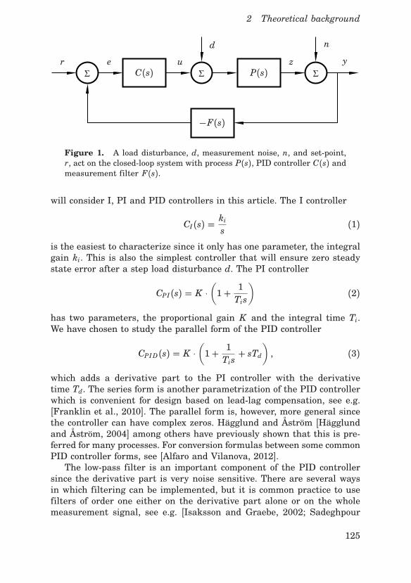
2 Theoretical background
ΣΣΣ
e u y
P(s)C(s)
−F(s)
d n
r z
Figure 1. A load disturbance, d, measurement noise, n, and set-point,r, act on the closed-loop system with process P(s), PID controller C(s) andmeasurement filter F(s).
will consider I, PI and PID controllers in this article. The I controller
CI(s) =ki
s(1)
is the easiest to characterize since it only has one parameter, the integralgain ki. This is also the simplest controller that will ensure zero steadystate error after a step load disturbance d. The PI controller
CPI(s) = K ⋅
(
1+ 1Tis
)
(2)
has two parameters, the proportional gain K and the integral time Ti.We have chosen to study the parallel form of the PID controller
CPID(s) = K ⋅
(
1+ 1Tis
+ sTd)
, (3)
which adds a derivative part to the PI controller with the derivativetime Td. The series form is another parametrization of the PID controllerwhich is convenient for design based on lead-lag compensation, see e.g.[Franklin et al., 2010]. The parallel form is, however, more general sincethe controller can have complex zeros. Hägglund and Åström [Hägglundand Åström, 2004] among others have previously shown that this is pre-ferred for many processes. For conversion formulas between some commonPID controller forms, see [Alfaro and Vilanova, 2012].The low-pass filter is an important component of the PID controller
since the derivative part is very noise sensitive. There are several waysin which filtering can be implemented, but it is common practice to usefilters of order one either on the derivative part alone or on the wholemeasurement signal, see e.g. [Isaksson and Graebe, 2002; Sadeghpour
125

Paper IV. Software-based optimal PID design
et al., 2012; Leva and Maggio, 2011; Kristiansson and Lennartson, 2002;Šekara and Mataušek, 2009]. An advantage with the measurement signalfilter is that one can design controllers for the combination P(s)F(s). Wehave thus chosen this approach, but decided to use a second-order filter
FPID(s) =1
(sT f )2/2+ sT f + 1, (4)
for PID control in order to guarantee amplitude roll-off for high fre-quencies. Some other studies [Larsson and Hägglund, 2011; Micić andMataušek, 2014; Garpinger, 2009; Romero Segovia et al., 2013] also ex-plore higher-order low-pass filters for PID control. For PI control we havechosen to use a first-order filter
FPI(s) =1
sT f + 1, (5)
also for the sake of high-frequency roll-off. The filter time constant T f isthe only parameter that needs to be set in both FPI and FPID . They wouldhave been more general with two or more parameters, but this form waschosen to keep the amount of controller parameters as low as possible.FPID has two complex poles with relative damping ζ = 1/
√2, which is the
smallest damping ratio for which there is no amplitude increase caused bythe filter. Larsson and Hägglund [Larsson and Hägglund, 2011] showedthat the filters FPI and FPID are well suited for the closed-loop system inFig. 1 and that filters of lower and higher order are not likely to give anyperformance benefits for equivalent noise sensitivity when using whiteGaussian noise. I control has natural roll-off, so FI(s) = 1.
2.3 Constrained optimization for PID design
Closed-loop requirements typically include specifications on load distur-bance attenuation, set-point tracking, robustness to process uncertaintyand measurement noise sensitivity. Set-point and load disturbance con-trol can be handled separately as shown in e.g. [Åström and Hägglund,2005]. Furthermore, Shinskey [Shinskey, 1996, p 11] indicates that mostset-points remain constant in continuous process control. For these tworeasons we have chosen to focus on load disturbance attenuation, robust-ness and noise sensitivity in this article, leaving the set-point r = 0.We choose to minimize the integrated absolute error (IAE)
IAE =∞∫
0
pe(t)pdt (6)
126

2 Theoretical background
during a unit step load disturbance, to optimize closed-loop performance.The variable t denotes time in [s] and the IAE-value is equal to the totalarea of the load disturbance response. Shinskey [Shinskey, 1996, p 17]points out that the IAE is a valuable performance measure since it canbe related to the economic cost of adding either too much or too little of anexpensive ingredient. Other criteria for control performance such as theintegrated square error, ISE, and the integrated time-weighted absoluteerror, ITAE, have also been suggested by e.g. [McMillan, 1983; Marlin,1995].According to e.g. [Åström and Hägglund, 2005, pp 112–116] and [Zhou
and Doyle, 1998, pp 142–143] robustness can be captured by the sensitivityfunction
S(s) = 11+ P(s)C(s)F(s) , (7)
and the complementary sensitivity function
T(s) = P(s)C(s)F(s)1+ P(s)C(s)F(s) . (8)
We choose to set robustness constraints on the maximum values of thesefunctions
pS(iω )p ≤ Ms, pT(iω )p ≤ Mt, ∀ω ∈ R+, (9)
where ω is the frequency in [rad/s] and R+ denotes the set of all non-
negative real numbers. As shown in [Åström and Hägglund, 2005, pp 116–117] this corresponds to the open-loop Nyquist curve of P(iω )C(iω )F(iω )not entering the Ms- or Mt-circles shown in Fig. 2. The circles expandwith decreasing values of Ms and Mt, resulting in greater closed-loop ro-bustness. Ms- and Mt-values ranging between 1.2 and 2.0 give reasonablerobustness and correspond to gain margins between 6 and 2, as well asphase margins between 49○ and 29○.Large control signal activity generated by measurement noise could
cause undesirable actuator wear and tear. The transfer function frommeasurement noise to control action is
Sc(s) =C(s)F(s)
1+ P(s)C(s)F(s) , (10)
and its impact depends on many factors, with the controller parametersand low-pass filter being particularly important. In this article we havechosen to constrain the H2-norm of Sc(s)
qSc(s)q2 ≤ κu, (11)
127
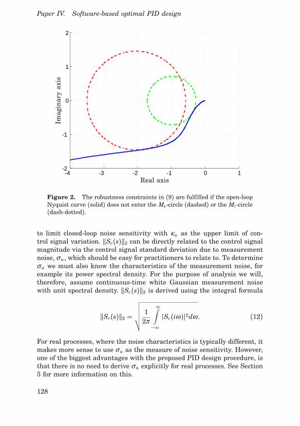
Paper IV. Software-based optimal PID design
-4 -3 -2 -1 0 1-2
-1
0
1
2
Imaginaryaxis
Real axis
Figure 2. The robustness constraints in (9) are fulfilled if the open-loopNyquist curve (solid) does not enter the Ms-circle (dashed) or the Mt-circle(dash-dotted).
to limit closed-loop noise sensitivity with κu as the upper limit of con-trol signal variation. qSc(s)q2 can be directly related to the control signalmagnitude via the control signal standard deviation due to measurementnoise, σu, which should be easy for practitioners to relate to. To determineσu we must also know the characteristics of the measurement noise, forexample its power spectral density. For the purpose of analysis we will,therefore, assume continuous-time white Gaussian measurement noisewith unit spectral density. qSc(s)q2 is derived using the integral formula
qSc(s)q2 =
√
√
√
√
√
12π
∞∫
−∞
pSc(iω )p2dω . (12)
For real processes, where the noise characteristics is typically different, itmakes more sense to use σu as the measure of noise sensitivity. However,one of the biggest advantages with the proposed PID design procedure, isthat there is no need to derive σu explicitly for real processes. See Section5 for more information on this.
128

2 Theoretical background
Taking all three criteria of performance, robustness and noise sensitiv-ity into consideration, we can now formulate a constrained optimizationproblem
minimizeK ,Ti,Td,T f∈R+
∞∫
0
pe(t)pdt,
subject to pS(iω )p ≤ Ms,pT(iω )p ≤ Mt, ∀ω ∈ R
+,
qSc(s)q2 ≤ κu,
(13)
which can be used to design any of the controllers C(s) given in Eqs. (1–3) as well as the filters in Eqs. (4–5). However, the non-convexity of thisoptimization problem makes it difficult to solve directly.
2.4 A software tool for robust PID design
A MATLAB®-based software tool for robust PID design was presented in[Garpinger and Hägglund, 2008]. This tool solves a modified version ofEq. (13) without the noise sensitivity constraint
minimizeK ,Ti,Td∈R+
∞∫
0
pe(t)pdt,
subject to pS(iω )p ≤ Ms,pT(iω )p ≤ Mt, ∀ω ∈ R
+,
pS(iω s)p = Ms, and/orpT(iω t)p = Mt,
(14)
where ω s are frequencies for which the open-loop frequency response istangent to the Ms-circle and vice versa for ω t and the Mt-circle. Eitherω s or ω t could be an empty set, but not simultaneously. As a direct resultof these additional equality constraints at least one of the inequality con-straints will be active, thus forcing the Nyquist curve to touch either oneor both robustness circles. This makes the optimization problem easier tosolve than the problem with only inequality constraints. The drawback isthat there could be a controller with greater robustness that yields betterperformance. Several studies by [Garpinger, 2009; Garpinger et al., 2014;Grimholt and Skogestad, 2012] do, however, indicate that the solutionto the optimization problem (14) is, in most cases, optimal also withoutequality constraints just as long as the robustness is reasonable with Msand Mt roughly below 1.8. The low-pass filter time constant, T f , is fixed inthis optimization problem such that we design controllers for the processand filter combination P(s)F(s).
129

Paper IV. Software-based optimal PID design
We have chosen to call this PID controller tuning method Software-based optimal robust design (SWORD). The software tool needs a stablelinear process model as well as specified values of Ms, Mt and T f to work.The optimization problem is solved using a simplex-based algorithm calledthe Nelder-Mead method, see e.g. [Walters et al., 1991; Lagarias et al.,1998]. The simplex propagates through the space of (Ti,Td) for PID controland (Ti) for PI control. The proportional gain K is chosen such that eachopen-loop Nyquist curve fulfills either or both equality constraints. TheIAE-value is derived through Simulink® simulations for every controllerthat the algorithm propagates through. More detailed descriptions of theprogram are given in [Garpinger, 2009; Garpinger and Hägglund, 2008].The software tool is freely available at:
http://www.control.lth.se/project/PID
2.5 A process batch for controller evaluation
A batch of 134 stable processes with monotonous step responses, represen-tative for the process industry, was presented in [Hägglund and Åström,2004]. These processes will be utilized here to show which types of pro-cesses have the greatest benefit of the derivative part of the PID con-troller. The nine different process types from the batch can be found inFig. 3, while the parameter values used are the same as in [Hägglund andÅström, 2004]. Each process has been assigned a symbol in the figure thatwill later be used in plots.Notice that the process gains will affect the value of qSc(s)q2. According
to [Shinskey, 1996, p 99] many processes have static gains in the range1−10. It is reasonable to believe, however, that integrating processes (likeP6) could have much smaller integral gains e.g. for large tanks. In thisarticle we have chosen to set both static and integral process gains to 1 forthe batch. Like the characteristics and intensity of the noise, we believethat these gains vary more or less randomly from process to process. In ourcontroller comparisons in Section 6, we will make conclusions with regardsto this assumption. However, processes with e.g. high noise intensity, asensitive actuator or small process gain, will always be more sensitive tonoise throughput.The processes in Fig. 3 will be approximated with first-order time-
delayed (FOTD) models
Pm(s) =Kp
sT + 1 e−sL, (15)
in order classify them using the normalized time delay,
τ = L
L + T , (16)
130

2 Theoretical background
P1 :e−s
1+ sT (○) P2 :e−s
(1+ sT)2 (+)
P3 :1
(s+ 1)(1+ sT)2 ($) P4 :1
(s+ 1)n (�)
P5 :3∏
i=0
1(1+α is) (◊), P6 :
e−sL1
s(1+ sT1)(∗)
P7 :e−sL1
(1+ sT)(1+ sT1)(J), P8 :
1−α s
(s+ 1)3 (⋆)
P9 :1
(s+ 1)((sT)2 + 1.4sT + 1) (✶)
Figure 3. Test batch of processes representative for the process industry.The parameter values used are the same as in [Hägglund and Åström,2004]. Notice that each type of process has been assigned a symbol inparenthesis.
which ranges from 0 to 1. We define a process as lag-dominated if 0 ≤ τ ≤0.2, balanced if 0.2 < τ < 0.7, and delay-dominated if 0.7 ≤ τ ≤ 1.0. TheFOTD model parameters have been derived through step response testsusing the 63%-rule, described in e.g. [Garpinger and Hägglund, 2014]. Inthis article we will mainly run SWORD with the actual process models,not the FOTD models. The principal reason for doing so is because wewant to analyze the control at its maximum potential, using other modelswould lead to comparisons that has as much to do with the modelingmethod as it has to do with controller design. In Section 5, however, wewill briefly comment on why the step response models should not be usedtogether with SWORD. For a more thorough discussion on modeling foroptimal PID control, see [Garpinger and Hägglund, 2014].We will use three processes from the batch to further analyze the
trade-offs between performance, robustness and noise sensitivity. The firstprocess
PI(s) =1
(s+ 1)(0.1s+ 1)(0.01s+ 1)(0.001s+ 1) , (17)
is lag-dominated (τ = 0.067), the second process
PI I(s) =1
(s+ 1)4 , (18)
131

Paper IV. Software-based optimal PID design
is balanced (τ = 0.33), and the third process
PI I I(s) =e−s
(0.05s+ 1)2 , (19)
is delay-dominated (τ = 0.93).
3. Performance and noise sensitivity trade-off
In Section 5 we suggest a PID design method where robustness is set toa fixed value M = Ms = Mt, with Ms equal to Mt for simplicity. For now,we will assume M = 1.4, see Section 4 for a discussion on how the ro-bustness level affects PID controller design. The filter time constant, T f ,is varied to create a set of controllers given by the SWORD method. Fig-ure 4 shows how the IAE-value depends on qSc(s)q2 for an example set ofPID controllers on the process PI I(s), (18). As pointed out in [Garpinger,2009], there is little to gain in terms of performance for small valueson T f , but it costs a lot in terms of noise sensitivity. For low values onqSc(s)q2 the opposite holds, where decreasing noise sensitivity quickly de-teriorates performance. A good trade-off between performance and noisesensitivity for the curve in Fig. 4 would be to choose the controller thatgives qSc(s)q2 ( 10. A different approach is to pick the controller that re-sults in a specified maximum allowed noise sensitivity, κu. Figure 5 showshow performance (top plot) and noise sensitivity (bottom plot) depend onT f . The filter has a major impact on the PID controller and the closed-loop performance for filter time constants roughly between T f = 0.1− 10.In discrete-time control, sampling will also act as a filter which will limitthe best possible performance and the maximum noise sensitivity, see e.g.[Garpinger, 2009].The transfer functions of the controller and filter combinations will be
CI , CPIFPI and CPIDFPID . As the filter time constant T f increases, thePID controller will gradually become similar to a PI controller, while thePI controller becomes similar to an I controller. The PI and PID formsare fundamentally different since the PI controller will not use a second-order filter and because it has no D-part. However, in order to simplifyour analysis we will say that the combination CPIDFPID becomes a PIcontroller when its proportional, derivative and filter parts
K ⋅ (1+ sTd) ⋅1
(sT f )2/2+ sT f + 1, (20)
have no phase greater than 0○, i.e. if
arctan(ωTd) − arctan(
ωT f1− 0.5ω 2T2f
)
≤ 0,∀ω ∈ R+. (21)
132

3 Performance and noise sensitivity trade-off
10-1
100
101
102
103
104
105
106
2
3
4
5
6
7
8
9
10
IAE
qSc(s)q2
T f = 0.01
T f = 100T f = 10
T f = 1T f = 0.1
Figure 4. Varying the filter time constant T f in SWORD, for a givenrobustness M = Ms = Mt, results in a set of controllers, in this case PID.For the balanced process PI I(s) and M = 1.4 both performance and noisesensitivity will decrease along the curve as the filter time constant T fincreases. Values of T f are indicated in the plot.
The phase will always be zero for ω = 0. The arctangent function ismonotonically increasing and the order of the filter is higher than thatof a PD controller. Thus, (21) is only true if the phase has no more zerocrossings, i.e. if
Td =T f
1− 0.5ω 2T2f, (22)
has no solution. Solving (22) with respect to ω gives
ω =√2T f
√
1− T fTd, (23)
which only has a solution ω > 0 if Td > T f . Therefore, our PID con-trollers will be called PI controllers if T f ≥ Td. Notice that Td ,= 0 whenthis happens. As T f increases, the PI and PID forms in (2) and (3) willeventually converge to the same I controller (1) when the zeros of thecontrollers cancel the poles of the filters. This effect can be seen in Fig. 5for the PID case, where the performance and noise sensitivity curves arealmost flat for T f > 10. Notice that the filter time constant for the PIcontroller will not be the same as for the PID controller at this point.
133

Paper IV. Software-based optimal PID design
10-2
10-1
100
101
102
2
3
4
5
6
7
8
9
10
IAE
T f
10-4
10-3
10-2
10-1
100
101
102
10-1
100
101
102
103
104
105
106
qSc(s)q2
T f
Figure 5. The relation of the filter time constant T f with performanceIAE (top) and noise sensitivity qSc(s)q2 (bottom) for the balanced processPI I(s) with M = 1.4 when SWORD is used to derive PID controllers.
134

3 Performance and noise sensitivity trade-off
10-1
100
101
3
4
5
6
7
8
9
10T fPID = 100
T fPID = 10
T fPID = 1
T fPI = 100
T fPI = 10
T fPI = 1
T fPI = 0.1
T fPI = 0.01
qSc(s)q2
IAE
Figure 6. Performance and noise sensitivity trade-offs for PI I(s) withM = 1.4, comparing the sets of PI (dashed) and PID controllers (solid)derived with the SWORD method. The green part of the PID curve showswhen they are defined as PI controllers, i.e. when T f ≥ Td. PI (left) andPID (right) values of T f are indicated in the plot.
In [Garpinger, 2009], optimal Youla parametrized controllers of highorder were derived for almost the same optimization problem as (13). Itwas shown that the optimal controller type depends on the maximum al-lowed noise sensitivity. Higher-order controllers are preferable for highernoise sensitivity, while PID, PI and even I controllers become optimal asthe maximum noise sensitivity limit is gradually decreased. It was alsoshown in the same thesis that for a certain value on qSc(s)q2, the PI con-trollers from SWORD become better than the PID controllers. Figure 6shows this effect, which stems from the different controller forms. Theset of PID controllers (3) are shown as the solid line in the figure, whilethe set of PI controllers (2) are given by the dashed line. The PID con-trollers become PI controllers (T f ≥ Td) almost at the same point as thePI form becomes better than the PID form, around qSc(s)q2 = 0.48. Asthe two controller sets approaches qSc(s)q2 = 0.29, they both converge tothe same I controller. If the noise sensitivity is still higher than specifiedat this point, we suggest that the user switch to an I controller and de-
135
Paper IV. Software-based optimal PID design
crease the integral gain ki until qSc(s)q2 is small enough. We will explainwhy in Section 4. The relative performance gain from using a PID con-troller depends on the maximum allowed noise sensitivity. If we can allowqSc(s)q2 = 10, the IAE-value for PI control is up to 80% higher than forPID control, while for qSc(s)q2 = 1 the IAE value is 16% higher. Thesetrade-off curves will help us determine which processes have the biggestbenefits from the D-part. They will also show us when to switch from PIDto PI, and finally from PI to I control.
4. Controller optimality and robustness level selection
The SWORD method is used to design PI and PID controllers with differ-ent values on T f . This is done by solving the optimization problem (14)with the given controller forms (2) and (3). But, how close to optimalwill the set of controllers be with respect to the full optimization problem(13) and how will different choices of the robustness level M affect thedesign? In Section 2.4 we have already reasoned why controllers that giveactive robustness constraints in most cases also give the same solutionas optimization without equality constraints. However, we still need toexamine how close the set of controllers with different T f and fixed ro-bustness M = Ms = Mt are to the optimal of (13) for different κu. Thelag-dominated, balanced and delay-dominated processes PI(s) − PI I I(s)(17–19) will be used to represent the batch of processes in Fig. 3, whichis motivated in [Garpinger et al., 2014]. Varying T f and M we can find allcontrollers that could possibly solve (13). To be sure we have found theoptimal controller, however, there are two conditions that needs to be ful-filled. First of all, the performance and noise sensitivity trade-off curvesshould be monotonically decreasing with qSc(s)q2, i.e. as T f decreases.Otherwise, we could miss controllers with both better performance andlower noise sensitivity unless we examine a set of controllers large enoughto find these local minima. Secondly, we should beware that the trade-offcurves do not intersect each other for different values on M , or else thereare controllers with higher robustness that give better performance for thesame noise sensitivity. To investigate whether or not we can expect anyof these two cases when using SWORD, we have chosen to plot the trade-off curves for PI(s) − PI I I(s) with the different robustness constraintsM = 1.2, 1.25, 1.3, 1.35, 1.4, 1.45, 1.5, 1.55, 1.6.We will define our controllers as PID controllers if they have the form
(3) and T f < Td. PID controllers with T f ≥ Td and PI controllers (2) willbe defined as PI controllers until they converge to the same I controller forhigh enough values on T f . Thereafter, all controllers will be I controllerswith different integral gains ki.
136
4 Controller optimality and robustness level selection
The top plot of Fig. 7 shows the nine, tightly packed, trade-off curvesfor the lag-dominated process PI(s). Blue dash-dotted curves indicate PIDcontrollers, green solid lines PI controllers, and red dashed curve I con-trollers. Notice that the IAE-value generally decreases as M increases.A closer look at the trade-off curves shows that they are all monoton-ically decreasing. Several of the curves with the highest M -values do,however, intersect each other when the PI controllers are close to becomeI controllers. The largest relative difference in performance due to theseintersections is found between the curves for M = 1.4 and 1.6. The latterhas an IAE-value 20% higher than the former at the qSc(s)q2-value whereit becomes an I controller. Even so, we think it is fair to say that almostall controllers derived in the nine sets are optimal or at least near optimalfor the full optimization problem (13).The trade-off curves for the balanced process PI I(s) are shown in the
middle plot of Fig. 7. Notice that the span of PI controllers is narrowerthan for the lag-dominated process in the top plot of Fig. 7. This indicatesthat we gain more from using the D-part on this balanced process. Similarto the lag-dominated process, all curves are monotonically decreasing withqSc(s)q2. Some curves still intersect each other, but they are both fewerand give less relative increase in IAE compared to PI(s).The delay-dominated process PI I I(s), has PID trade-off curves that
are not monotonically decreasing. While this can be handled with oursuggested method by collecting a large enough set of controllers, we havechosen to only consider the trade-off curves given by PI and I controllers.Several studies have reported that derivative action has practically nobenefit for delay-dominated processes, see e.g. [Hägglund and Åström,2004], and we will add further evidence to this standpoint in Section 6.The nine trade-off curves for PI I I(s) are presented in the bottom plotof Fig. 7. Notice that the highest obtainable noise sensitivity is naturallylower than for PID controllers. All nine trade-off curves are monotonicallydecreasing and the relative IAE loss due to intersecting curves is lowerthan for both PI(s) and PI I(s).Given the three examples, we now conclude that our suboptimal rou-
tine for the optimization problem (13) gives either optimal or close to op-timal control for these three processes representing lag-dominated, bal-anced and delay-dominated processes. At least for the case with whiteGaussian noise. Figure 7 also reveals that trade-off curves for higherrobustness are generally above those for lower robustness. This meansthat M should always be set as high as possible to optimize performance,given that the user can still feel comfortable with the choice. Notice thatthe qSc(s)q2-value for which the PID to PI controller transition occursdecreases as the robustness increases. This has to do with the PID con-trollers having lower gains for higher robustness.
137

Paper IV. Software-based optimal PID design
10-1
100
101
102
10-2
10-1
100
101
102
replacements
qSc(s)q2
IAE
PI(s) - Lag-dominated dynamics
10-1
100
101
102
100
101
102
qSc(s)q2
IAE
PI I(s) - Balanced dynamics
10-1
100
101
100
101
102
qSc(s)q2
IAE
PI I I(s) - Delay-dominated dynamics
Figure 7. Performance and noise sensitivity trade-off curves for theprocesses PI(s) (top), PI I(s) (middle) and PI I I(s) (bottom) with M =1.2, 1.25, 1.3, ..., 1.6. Blue dash-dotted curves indicate PID controllers, greensolid lines show PI controllers and red dashed curves I controllers. Noticethat the trade-off curves with higher relative IAE-values have lower rela-tive values on M .
138

5 PID design procedure
5. PID design procedure
In this section we will introduce our proposed software-based PID designmethod for real processes. Given the information in Sections 3 and 4, wesuggest the following procedure:
1. Determine a process model and specify a maximum allowed robust-ness measure M = Ms = Mt. For example M = 1.4.
2. Find an initial controller along the trade-off curve and employ it onthe process.
3. Derive a set of controllers along the trade-off curve by adjusting T ffor PI and PID control and ki for I control.
4. Use e.g. a control knob for online selection of controllers along theset until finding the best controller that keeps the high-frequencycontrol signal variations below a maximum allowed level.
The same set of controllers can be used to detune the controller if it isdeemed too aggressive. Here we suggest use of the SWORD method tofind the set of controllers, but it should be possible to use roughly thesame steps with other methods, e.g. the one presented in [Hast et al.,2013]. Steps 1–3 should be easy enough to automate, but the fourth step ispreferably carried out manually. The initial controller could be determinedin several ways. If the process is either lag-dominated or delay-dominatedone option is to start with the I controller that gives the chosen robustnessM . If the process is balanced, one can instead find the best PI controlleralong the trade-off curve, i.e. at the transition to PID controllers. The setof controllers could initially contain somewhere between 10 to 20 differentcontrollers, with the possibility to expand it if desired. It can be expectedto take somewhere between 2–10 minutes to find the entire set of con-trollers with SWORD on a computer with reasonable performance. If theset of controllers is dense enough, parameters could also be interpolatedin order to derive a continuous set of parameters. The final controllercan be chosen either by visual feedback of the control signal level or byfinding a controller for which the losses in performance and noise sen-sitivity are balanced. There should also be some information to the useron how much of the nominal performance is lost when selecting differentcontrollers from the set.We will illustrate the design procedure with an example. Assume that
we want to find a controller for the balanced process PI I(s) that givesgood closed-loop performance with the constraints that M = 1.4 and thecontrol signal amplitude should be roughly below 5. Using SWORD onPI I(s) we derive an initial PID controller with T f = 0.5, called PID1.
139

Paper IV. Software-based optimal PID design
Table 1. A set of PID, PI and I controller parameters derived for theprocess PI I(s) using the constraint M = 1.4 in SWORD.
Controller K Ti Td ki T f IAE qScq2PID1 0.84 2.32 1.36 - 0.50 3.47 3.31PID2 0.72 2.39 1.43 - 0.78 4.10 1.61PID3 0.59 2.59 1.75 - 1.50 5.40 0.70PI1 0.39 2.57 - - 1.00 7.34 0.40PI2 0.47 4.29 - - 3.70 9.10 0.31I1 - - - 0.05 - 20.00 0.17
The reason for choosing an initial PID is just to show monotonous de-creases in both control signal activity and control performance. The topplot of Fig. 8 shows the performance and noise sensitivity trade-off plot forPI I(s). PID1 is marked with the blue triangle furthest to the right in thetrade-off curve. This controller results in the solid blue load disturbanceresponse in the middle plot and the control signal noise response furthestto the left (0–200 seconds) in the bottom plot. The measurement noise re-sponse was simulated in MATLAB® Simulink® using band-limited whitemeasurement noise with unit spectral density and a sampling period ofh = 0.01 seconds. From this response, we see that the control signal am-plitude is greater than our specification allows. Next we derive five morecontrollers, two PID controllers with T f = 0.78 (PID2) and T f = 1.50(PID3), two PI controllers with T f = 1.00 (PI1) and T f = 3.7 (PI2), aswell as an I controller (I1) with ki = 0.05. This gives us a total set of sixcontrollers with the parameters, IAE and qSc(s)q2-values given in Table 1.In Fig. 8 (top plot) the PID controllers are marked with blue triangles,PI controllers with green squares and the I controller with a red circle.The load disturbance responses are collected in the middle plot with thesame color scheme as the top plot. I1, PI1 and PID1 are marked with solidlines, PI2 and PID2 with dash-dotted lines, while PID3 is marked with adashed line. The measurement noise responses are shown within the timeintervals: 0− 200 (PID1), 200− 400 (PID2), 400− 600 (PID3), 600− 800(PI1), 800−1000 (PI2), and 1000−1200 seconds (I1). Since PID2 satisfiesour noise sensitivity specification of a control signal amplitude roughlybelow 5, we finally select this controller for our process.Notice that we have used a perfect model of PI I(s) in the example. In
[Garpinger and Hägglund, 2014], it was pointed out that SWORD shouldnot be combined with FOTD models derived from step responses, as de-scribed in the same paper. For the process batch in Fig. 3, such modelsresult in robustness values on Ms and Mt between 1.4− 2.3 for the choiceof M = 1.4. For the previous example, the resulting Ms-values would be
140

5 PID design procedure
10-1
100
101
0
5
10
15
20
25
30
qSc(s)q2
IAE
Trade-off plot
0 20 40 60 80 100
0
0.2
0.4
0.6
0.8
1
Time (s)
Controlerror
Load disturbance responses
0 200 400 600 800 1000 1200-15
-10
-5
0
5
10
15
Time (s)
Controlsignal
Measurement noise responses
PID1
PID2PID3 PI1 PI2 I1
Figure 8. Given the process PI I(s) and the constraint M = 1.4, theperformance and noise sensitivity trade-off curve is shown in the top plotwhere the six different controllers in Table 1 are marked with triangles(PID), squares (PI) and a circle (I). The load disturbance and control signalnoise responses are shown in the middle and bottom plots respectively. PIDcontrollers are shown in blue, PI controllers in green and the I controllerin red. From this information, the user can select the best performingcontroller that gives the maximum acceptable noise sensitivity.
141

Paper IV. Software-based optimal PID design
1.70 (PID1), 1.65 (PID2), 1.58 (PID3), 1.55 (PI1), 1.47 (PI2), 1.17 (I1).In [Garpinger and Hägglund, 2014], it is also shown that the same stepresponse models work poorly together with PID tuning rules like Lambdatuning [Dahlin, 1968], AMIGO [Hägglund and Åström, 2004] and SIMC[Skogestad, 2003]. It is thus highly desirable to find modeling methodsthat work well together with PID design methods.
6. Benefits of the derivative part
As we could see in Fig. 7, the qSc(s)q2-values for which the transitionsbetween PID, PI and I controllers occur depends on the process and therobustness constraints. To investigate which processes have the most togain from using the D-part of the PID controller, we will assume a ro-bustness of M = 1.4 and examine where the controller transition fromPI to PID occurs for the processes in Fig. 3. We will also compare theperformance of the PI and PID controllers for qSc(s)q2 = 0.7, 2, 10, whichwill be referred to as low, medium and high noise sensitivity respectively.Hägglund and Åström [Hägglund and Åström, 2004] used the in-
tegrated errors of PI and PID controllers derived with the method in[Panagopoulos et al., 2002] to show which processes in the test batch havethe most to gain from using the derivative part. This study showed thatlag-dominated processes have the most to gain from using the D-partalthough the variation in relative performance increase is large. Thesecontrollers were, however, designed without any filter or noise sensitivityconstraint. A PID/PI performance plot, similar to the one in [Hägglundand Åström, 2004], could be made with SWORD if it is run with low valueson the filter time constant T f , but we believe that the addition of a noisesensitivity constraint is the key to reveal when the control really benefitsfrom the D-part. Figure 9 shows how the value of qSc(s)q2 for which thePI controller is as good as the PID controller, qSc(s)q2 = κ eq, varies withnormalized time delay τ over the process batch. Most processes seem tofollow the same general pattern that κ eq increases as τ decreases. Thisshows that many lag-dominated processes should be controlled with PIcontrollers even if we can allow relatively high values on the noise sensi-tivity. There are, however, some processes that deviate from this pattern.The integrating processes in P6 with τ = 0 have low values on κ eq, sug-gesting that they have a lot to gain from the D-part. The second-ordertime-delayed processes with identical poles, P2 in the same figure, obtainthe smallest values on κ eq as τ decreases. This indicates that they too willbenefit a lot from the D-part. The processes in P3 that resembles second-order processes, P4, and P8 with larger values on α also have slightlylower κ eq than most other processes.
142

6 Benefits of the derivative part
0 0.2 0.4 0.6 0.8 110
-2
10-1
100
101
102
103
τ
κeq
Figure 9. Variation of the noise sensitivity for which PI controllers per-form equally well to PID controllers, qSc(s)q2 = κ eq, with normalized timedelay τ . The different symbols are associated with the processes of thebatch as shown in Fig. 3.
The SWORD method gives either a PI or a PID controller and it isuseful to know when to switch from PID to PI form. Figure 10 showshow T f /Td, for which the PI form in (2) performs equally well to thePID form (3), varies with normalized time delay τ . The function f (τ ) =0.43τ 2 + 0.45τ + 0.78 is marked as a dashed green line in the figure andprovides a lower limit for the test batch. If the ratio between T f and Tdsurpasses this function, one should start comparing PID controllers withPI controllers or perhaps even switch over to PI control altogether.While Fig. 9 indicates which processes have the best potential to ben-
efit from the D-part, it says nothing about the relative performance gainone can expect when going from PI to PID. To give a measure of this, wehave calculated the IAE-values of the PI and PID controllers for three spe-cific noise sensitivities, qSc(s)q2 = 0.7, 2 and 10. These will correspond tolow, medium and high noise sensitivity. This study covers the whole testbatch, but we will start by looking at the process types P1 and P2. Fig-ure 11 shows the relative performance loss in using PI control comparedto PID control for the first-order time-delayed processes P1. The circlesalong the red line show the ratios for qSc(s)q2 = 0.7, the green squaresshow the same for qSc(s)q2 = 2, and the blue triangles show the benefitsfor qSc(s)q2 = 10. For the low noise sensitivity, there is nothing to gain forany of the processes in P1. With medium noise sensitivity, processes with
143
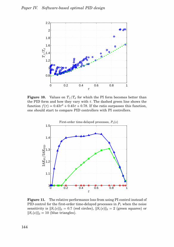
Paper IV. Software-based optimal PID design
0 0.2 0.4 0.6 0.8 1
0.8
1
1.2
1.4
1.6
1.8
2
2.2
τ
Tf/Td
Figure 10. Values on T f /Td for which the PI form becomes better thanthe PID form and how they vary with τ . The dashed green line shows thefunction f (τ ) = 0.43τ 2 + 0.45τ + 0.78. If the ratio surpasses this function,one should start to compare PID controllers with PI controllers.
0 0.2 0.4 0.6 0.8 11
1.1
1.2
1.3
1.4
1.5
τ
IAEPI/IAEPID
First-order time-delayed processes, P1(s)
Figure 11. The relative performance loss from using PI control instead ofPID control for the first-order time-delayed processes in P1 when the noisesensitivity is qSc(s)q2 = 0.7 (red circles), qSc(s)q2 = 2 (green squares) orqSc(s)q2 = 10 (blue triangles).
144

6 Benefits of the derivative part
0 0.2 0.4 0.6 0.8 110
0
101
τ
IAEPI/IAEPID
Second-order time-delayed processes, P2(s)
Figure 12. The relative performance loss from using PI control insteadof PID control for the second-order time-delayed processes in P2 whenthe noise sensitivity is qSc(s)q2 = 0.7 (red circles), qSc(s)q2 = 2 (greensquares) or qSc(s)q2 = 10 (blue triangles). Notice the logarithmic scale forthe performance ratio.
τ = 0.3 − 0.9 have the most to gain from using the D-part. The relativegains are, however, rather low for all processes. The process with τ = 0.77has the biggest performance loss ratio, with its PI controller having 30%worse IAE than the PID controller. For the high noise sensitivity, pro-cesses with τ = 0.1− 0.8 have the most use of the D-part. This covers thewhole field of balanced processes. The highest relative losses in IAE fromPID to PI are, however, still quite modest. It is obvious from looking atFig. 11, that the most lag-dominated and delay-dominated processes havevery little to gain from using the D-part. These lag-dominant processescould, however, benefit from the D-part if the noise sensitivity is allowedto be very high. Given that PI control is not more than 43% worse thanPID control for any of the processes with any of the three noise sensitivi-ties, one could argue that PI control could be used for all processes withessentially first-order time-delayed dynamics unless noise is not an issue.Figure 12 shows the relative performance losses for second-order pro-
cesses with identical poles, P2. The processes and relative noise sensi-tivities are marked with the same signs and color schemes as in Fig. 11.Notice the logarithmic scale for the performance loss ratio. For τ = 0.5−1,the three curves are similar to those for P1, although there is now also aslight benefit in going from PID to PI for the low noise sensitivity. The
145
Paper IV. Software-based optimal PID design
main difference between process type P1 and P2 is, however, what happensfor the most lag-dominated second-order processes. For qSc(s)q2 = 0.7,there is as much as a 225% performance loss in using PI controllers in-stead of PID. The same numbers for qSc(s)q2 = 2 and 10 are 464% and1590% respectively. This shows that process dynamics with two identi-cal poles and small relative time delay have a lot to gain from using theD-part.Figure 13 displays how IAEPI/IAEPID varies over the whole test batch
in Fig. 3, for qSc(s)q2 = 0.7 (top plot), qSc(s)q2 = 2 (middle plot) andqSc(s)q2 = 10 (bottom plot). Notice the different scales for the perfor-mance loss ratios. As expected, process types P2 and P6 stand out of allthree plots as those where PID control is the most beneficial. We have al-ready described the pattern for P2 and for P6 the processes with least timedelay give the largest performance loss ratios. Notice, however, that forintegrating processes with low values on the integral gain, this effect willbe much smaller. These could be compared with the most lag-dominatedprocesses in P1 if these are approximated as integrating processes withKv = 1/T . For low noise sensitivity, process types P4 and P8 also standout as those where PID is preferred. For the rest of the process types thereis more of a general pattern that differs over the three noise sensitivities.The conclusions are, however, pretty much the same as those for P1 alone.Lag- and delay-dominated processes, besides P2 and P6, have little to gainfrom using PID control. Processes roughly in the interval τ = 0.1 − 0.8have somewhat more to gain, but for processes with requirements on lownoise sensitivity there seems to be generally little to gain from using theD-part. Second-order processes with similar poles and little time delay aswell as second-order integral processes are, however, worthwhile to designPID controllers for even in these cases.
7. Conclusions and discussion
In this article, we have stated a non-convex optimization problem (13) fordesign of optimal PID controllers with respect to robustness and noisesensitivity constraints. We have also shown how to derive optimal or nearoptimal controllers for this problem by repeated use of a MATLAB®-basedsoftware method called SWORD. Variation of the noise filter time con-stant, its order and the controller form for the least acceptable robust-ness, lead to a set of PID, PI and I controllers which the user can switchbetween until the control signal activity is acceptable. This way, the op-timization can be handled without any noise modeling. The same set ofcontrollers can also be used to detune the controller if it is deemed tooaggressive for the actuator. Even though we have chosen to only use our
146

7 Conclusions and discussion
0 0.2 0.4 0.6 0.8 11
1.2
1.4
1.6
1.8
2
2.2
2.4
replacements
τ
IAEPI/IAEPID
qSc(s)q2 = 0.7
0 0.2 0.4 0.6 0.8 11
1.5
2
2.5
3
3.5
4
4.5
5
τ
IAEPI/IAEPID
qSc(s)q2 = 2
0 0.2 0.4 0.6 0.8 110
0
101
τ
IAEPI/IAEPID
qSc(s)q2 = 10
Figure 13. The relative performance loss from using PI control insteadof PID control for the test batch in Fig. 3 when the noise sensitivity isqSc(s)q2 = 0.7 (top plot), qSc(s)q2 = 2 (middle plot) or qSc(s)q2 = 10(bottom plot). Notice the different scales for the performance loss ratios,especially the logarithmic scale in the bottom plot. The different symbolsare associated with the processes as shown in Fig. 3.
147

Paper IV. Software-based optimal PID design
own PID design tool in this study, it seems reasonable to believe that thesame method could also work with other toolboxes like those presented ine.g. [Oviedo et al., 2006; Harmse et al., 2009; Sadeghpour et al., 2012].The H2-norm of the sensitivity function between measurement noise
and control signal is used as a measure of the closed-loop noise sensitivity.We show that by deriving the PI and PID controllers that give equivalentnoise sensitivity, one can compare how useful the derivative part is for acertain process. A batch of processes representative for the process indus-try was used to highlight some types of processes that benefit more fromthe D-part as well as some processes that benefit less. The same methodshould also work to determine which processes gain the most from us-ing even higher-order controllers if the PI controllers are exchanged fore.g. optimal Youla parametrized controllers derived in the same way asin [Garpinger, 2009]. From our study of PI and PID controllers, one canconclude that the optimal controller type depends on both the maximumallowed noise sensitivity of the closed-loop system and the process dynam-ics. For example, many lag-dominated processes benefit very little fromthe D-part unless the noise sensitivity is allowed to be very high. In ac-cordance with other studies, delay-dominated processes are also shown tohave little use of the D-part, even for high values on the noise sensitivity.Balanced processes have more to gain from the derivative action. How-ever, of the processes examined the two process types that have shown tohave the biggest benefit of the D-part are:
• Second-order processes with two identical poles and small relativetime delay.
• Second-order integrating processes with high integral gain and littledelay.
These two process types are both lag-dominated, which separate themfrom the rest of the lag-dominated processes that benefit less from theD-part. We believe that this has to do with the difference in relative orderbetween the processes since the other lag-dominated processes are essen-tially first-order systems. For this reason there seems to be room for aneven better classification of process dynamics than what can be done withthe normalized time delay, τ . The fact that PID control is superior to PIfor these two process types also makes it highly desirable to be able todistinguish them from other processes. There should be a lot to gain fromusing the D-part on these processes even if non-optimal control design isused.Tuning rules, like Lambda and IMC tuning, are the most commonly
used methods for systematic PID tuning in the process industry. In thisarticle we have proposed a new software-based optimal design method for
148

7 Conclusions and discussion
Table 2. Pros and cons of software-based tuning and tuning rules
Tuning Rules Software Tuning
Pros 1. Fast 1. Optimality2. Intuitive 2. Three criteria3. Easy to use 3. Pedagogic tool
Cons 1. Less than three criteria 1. Need better models2. Not optimal 2. Need autotuning
3. Poor availability
PID controllers and in Table 2 we have summarized some of the most im-portant advantages (pros) and disadvantages (cons) of both tuning rulesand software-based optimal design. Tuning rules have the advantagesthat they are fast, intuitive and simple to use, at least the ones mentioned.These properties make them popular in the process industry where gen-eral control knowledge often is poor and there is little time to spend ontuning each loop. It is, on the other hand, very difficult to capture allthree criteria of performance, robustness and noise sensitivity in just acouple of simple formulas and they can thus be quite far from optimal,see e.g. [Garpinger et al., 2014]. As soon as the complexity and numberof tuning rules needed to tune a process increase, people will stop usingthem. Tuning rules are thus not so suitable for design of controllers withderivative action and a low-pass filter. As we have shown in this arti-cle, software-based optimal design methods are able to provide optimalcontrollers with respect to performance, robustness and noise sensitivity.They are also pedagogic tools that can help us understand PID design bet-ter, for example by showing which processes benefit the most from the D-part. In [Garpinger and Hägglund, 2014] we also showed that optimal PIDcontrol design needs better models than what is typically given in processindustry today. The level of control knowledge needed to understand anduse software-based optimal design methods together with this demand onmore accurate models make us believe that the methods should ratherbe part of a new generation of autotuners than stand-alone methods. Thelack of such tools in industry rules out current use of software-based op-timal design methods, at least on a broader scale. We do, however, believethat the development potential is much greater for software-based opti-mal design than for tuning rules and that the key to success in the fieldis to find fast modeling tools that provide just enough process knowledgeto work with optimal control design, see [Garpinger and Hägglund, 2014].For these reasons, we believe that easy to use software tools for optimalcontroller design will be the future for PID control rather than tuningrules.
149
Paper IV. Software-based optimal PID design
8. Acknowledgements
This study was partly funded by the Swedish Foundation for Strategic Re-search through the PICLU center. The authors are members of the LCCCLinnaeus Center and the ELLIIT Excellence Center at Lund University.
References
Alcántara, S., R. Vilanova, and C. Pedret (2013). “PID control in termsof robustness/performance and servo/regulator trade-offs: A unifyingapproach to balanced autotuning”. Journal of Process Control 23:4,pp. 527–542.
Alfaro, V. M. and R. Vilanova (2012). “Conversion Formulae and Per-formance Capabilities of Two-Degree-of-Freedom PID Control Algo-rithms”. In: 17th. IEEE Conference on Emerging Technologies & Fac-tory Automation (ETFA). IEEE. Krakow, Poland.
Alfaro, V. M. and R. Vilanova (2013). “Performance and Robustness Con-siderations for Tuning of Proportional Integral/Proportional IntegralDerivative Controllers with Two Input Filters”. Industrial & Engineer-ing Chemistry Research 52:51, pp. 18287–18302.
Åström, K. J. and T. Hägglund (2005). Advanced PID Control. ISA – TheInstrumentation, Systems, and Automation Society, Research TrianglePark, NC.
Åström, K. J., H. Panagopoulos, and T. Hägglund (1998). “Design ofPI Controllers based on Non-Convex Optimization”. Automatica 34:5,pp. 585–601.
Dahlin, E. B. (1968). “Designing and tuning digital controllers”. Instru-ments and Control Systems 41:6, pp. 77–83.
Franklin, G. F., J. D. Powell, and A. Emami-Naeini (2010). Feedback Con-trol of Dynamic Systems. 6th Edition. Pearson, Upper Saddle River,NJ.
Garpinger, O. and T. Hägglund (2008). “A Software Tool for Robust PIDDesign”. In: 17th IFAC World Congress. Seoul, South Korea.
Garpinger, O. (2009). Design of Robust PID Controllers with ConstrainedControl Signal Activity. Licentiate Thesis ISRN LUTFD2/TFRT--3245--SE. Department of Automatic Control, Lund University, Swe-den.
Garpinger, O. and T. Hägglund (2014). “Modeling for Optimal PID De-sign”. In: 19th IFAC World Congress. Cape Town, South Africa.
150

References
Garpinger, O., T. Hägglund, and K. J. Åström (2014). “Performance androbustness trade-offs in PID control”. Journal of Process Control 24:5,pp. 568–577.
Grimholt, C. and S. Skogestad (2012). “Optimal PI-Control and Verifica-tion of the SIMC Tuning Rule”. In: IFAC Conference on Advances inPID Control. Brescia, Italy.
Hägglund, T. and K. J. Åström (2004). “Revisiting the Ziegler-Nichols stepresponse method for PID control”. Journal of Process Control 14:6,pp. 635–650.
Harmse, M., R. Hughes, R. Dittmar, H. Singh, and S. Gill (2009). “Ro-bust optimization-based multi-loop PID controller tuning: A new tooland an industrial example”. In: 7th IFAC International Symposiumon Advanced Control of Chemical Processes, ADCHEM’09. Istanbul,Turkey.
Hast, M., K. J. Åström, B. Bernhardsson, and S. P. Boyd (2013). “PIDdesign by convex-concave procedure”. In: 2013 European Control Con-ference. Zürich, Switzerland.
Isaksson, A. and S. Graebe (2002). “Derivative filter is an integral part ofPID design”. Control Theory and Applications, IEE Proceedings 149:1,pp. 41–45.
Kristiansson, B. and B. Lennartson (2002). “Robust and optimal tuningof PI and PID controllers”. Control Theory and Applications, IEE Pro-ceedings D 149:1, pp. 17–25.
Kristiansson, B. and B. Lennartson (2006). “Evaluation and simple tuningof PID controllers with high-frequency robustness”. Journal of ProcessControl 16 (2), pp. 91–102.
Lagarias, J. C., J. A. Reeds, M. H. Wright, and P. E. Wright (1998).“Convergence properties of the Nelder-Mead simplex algorithm in lowdimensions”. SIAM Journal on Optimization 9, pp. 112–147.
Larsson, P.-O. and T. Hägglund (2011). “Control Signal Constraints andFilter Order Selection for PI and PID Controllers”. In: 2011 AmericanControl Conference. San Francisco, California, USA.
Leva, A. and M. Maggio (2011). “A systematic way to extend ideal PIDtuning rules to the real structure”. Journal of Process Control 21:1,pp. 130–136.
Marlin, T. (1995). Process Control – Designing Processes and Control Sys-tems for Dynamic Performance. Chemical Engineering. McGraw-Hill,New York, USA.
McMillan, G. (1983). Tuning and Control Loop Performance. ISA, Re-search Triangle Park, NC.
151

Paper IV. Software-based optimal PID design
Micić, A. D. and M. R. Mataušek (2014). “Optimization of PID con-troller with higher-order noise filter”. Journal of Process Control 24:5,pp. 694–700.
Nordfeldt, P. and T. Hägglund (2006). “Decoupler and PID controller de-sign of TITO systems”. Journal of Process Control 16:9, pp. 923–936.
Oviedo, J. J. E., T. Boelen, and P. van Overschee (2006). “Robust AdvancedPID Control (RaPID) - PID Tuning Based on Engineering Specifica-tions”. IEEE Control Systems Magazine 26, pp. 15–19.
Panagopoulos, H., K. J. Åström, and T. Hägglund (2002). “Design of PIDcontrollers based on constrained optimisation”. IEE Proceedings - Con-trol Theory & Applications 149:1, pp. 32–40.
Rivera, D. E., M. Morari, and S. Skogestad (1986). “Internal Model Con-trol. 4. PID Controller Design”. Ind. Eng. Chem. Process Des. Dev. 25,pp. 252–265.
Romero Segovia, V., T. Hägglund, and K. J. Åström (2013). “Noise fil-tering in PI and PID Control”. In: 2013 American Control Conference.Washington, D.C., USA.
Romero Segovia, V., T. Hägglund, and K. J. Åström (2014a). “Designof measurement noise filters for PID control”. In: 19th IFAC WorldCongress. Cape Town, South Africa.
Romero Segovia, V., T. Hägglund, and K. J. Åström (2014b). “Measure-ment noise filtering for PID controllers”. Journal of Process Control24:4, pp. 299–313.
Sadeghpour, M., V. de Oliveira, and A. Karimi (2012). “A toolbox for robustPID controller tuning using convex optimization”. In: IFAC Conferenceon Advances in PID Control. Brescia, Italy.
Shinskey, F. G. (1996). Process-Control Systems. Application, Design, andTuning. 4th. McGraw-Hill, New York, NY.
Skogestad, S. (2003). “Simple analytic rules for model reduction and PIDcontroller tuning”. Journal of Process Control 13:4, pp. 291–309.
Šekara, T. B. and M. R. Mataušek (2009). “Optimization of PID controllerbased on maximization of the proportional gain under constraints onrobustness and sensitivity to measurement noise”. IEEE Transactionson Automatic Control 54:1, pp. 184–189.
Walters, F. H., L. R. Parker Jr, S. L. Morgan, and S. N. Deming (1991).Sequential Simplex Optimization. CRC Press LLC.
Zhou, K. and J. Doyle (1998). Essentials of Robust Control. Prentice HallInternational, Upper Saddle River, NJ.
152

Paper V
Cascade control of the friction stirwelding process to seal canisters for
spent nuclear fuel
Lars Cederqvist Olof Garpinger Tore HägglundAnders Robertsson
Abstract
This article presents the development to reliably seal copper canisterscontaining the Swedish nuclear waste, using friction stir welding. Toavoid defects and welding tool fractures, it is important to control thewelding temperature within a span of 790 to 910○C. A cascade con-troller is used to efficiently suppress fast power input disturbancesreducing their impact on the temperature. The controller is tuned us-ing a recently presented method for robust PID control. Results showthat the controller keeps the temperature within ±10○C during the40 minute long joint line sequences. Apart from the cascaded controlstructure, good process knowledge and control strategies adapted todifferent weld sequences have contributed to the successful results.
©2012 Elsevier. Reprinted, with permission, from Control EngineeringPractice, 20:1, pp. 35–48, 2012.
153

Paper V. Cascade control of the friction stir welding process
Figure 1. Protection barriers in the Swedish method for nuclear wastemanagement.
1. Introduction
1.1 Background
The Swedish Nuclear Fuel and Waste Management Company (SKB) plansto join at least 12,000 lids and bases to the extruded copper tubes con-taining Sweden’s nuclear waste, using friction stir welding (FSW) as de-scribed by [Thegerström, 2004]. The canisters produced (5 m height, 1 mdiameter, made out of oxygen-free copper) are a major component of theSwedish system for managing and disposing of radioactive waste. Theywill be stored in the Swedish bedrock and must remain intact for 100,000years. A corrosion barrier of 5 cm thick copper and a cast iron insert formechanical strength are used to meet this requirement. Figure 1 illus-trates the barriers that will jointly prevent the radioactive substances inspent fuel from spreading into the environment.To ensure that high quality welds are produced repeatedly during more
than 40 years of production, there is an evident need for automated weld-ing instead of the past procedure depending on a skilled welding operator.A correctly tuned controller will not only be able to react to process dis-turbances faster, but also produce a more reliable process throughout theapproximately 45 minute long weld cycles.
1.2 Friction stir welding
FSW is a thermo mechanical solid-state process that was invented in 1991at The Welding Institute (TWI) in Cambridge, England [Thomas et al.,
154

2 Process description
Figure 2. Illustration of the friction stir welding process to seal coppercanisters.
1991]. A rotating non-consumable tool, consisting of a tapered probe andshoulder, is plunged into the weld metal and traversed along the joint line,see Fig. 2. For thick section welds (e.g. the copper canisters), a pilot holehas to be drilled to make the plunge sequence possible without significantprobe wear. Frictional heat is generated between the tool and the weldmetal, causing the metal to soften, normally without reaching the meltingpoint, and allowing the tool to traverse the joint line. Deeper knowledgeof FSW and its applications in industry can be gained from reading e.g.[Mishra and Mahoney, 2007], [Nandan et al., 2008] and [Lohwasser andChen, 2009].
2. Process description
2.1 Technical data
In 2003, a purpose-built machine from ESAB was installed at SKB’s Can-ister laboratory in Oskarshamn (see Fig. 3). In this machine, the weldinghead rotates up to 425 degrees around the canister, which is clamped witha force of 3200 kN. The lid is pressed down with a force of 390 kN.All welds are carried out under force control, i.e. constant axial force
(input 3 in Fig. 2) throughout the weld cycle. For more information onthe machine, see e.g. [Ronneteg et al., 2006].
2.2 Available control and measurement signals
One reason for the fast (and growing) implementation of FSW in industryis that the method has few input variables. The input parameters, thatcan be modified during the copper canister welds, are listed according toFig. 2; 1. tool rotation rate, 2. welding speed along the joint, and 3. axial
155

Paper V. Cascade control of the friction stir welding process
Figure 3. Purpose-built FSW machine for copper canister welding.
force (controls the position of the tool in relation to the canister surface,i.e. the tool depth). The measured variables are the welding (tool) temper-ature, the torque required by the spindle (that drives the tool rotation) tomaintain the tool rotation rate, and the depth of the tool into the weldedmaterial.There are also some elementary relationships between the signals that
are important to understand. The tool rotation rate multiplied with thespindle torque is equal to the power input in units of kW. In additionto this, the heat input (J/mm) can be derived by dividing the power in-put with the welding speed. Both quantities are closely correlated to thewelding (tool) temperature.
2.3 Argon shielding gas
[Upadhyay and Reynolds, 2010] investigated the effects of varying thermalboundary conditions by for example, welding under water. Similarly, theprocess stabilizing effect that argon gas has on the copper canister welds,was described by [Cederqvist et al., 2010a]. Today, all welds are producedin argon gas by placing a gas chamber over the tool. The main reasons forusing argon as a shielding gas are to achieve a weld zone with minimaloxide inclusions and to get a more robust process, partly thanks to lessshoulder wear. As a direct result of this, the spindle torque variationsare smaller and the controller will thus have an easier task obtaining itsobjectives.
156

2 Process description
Figure 4. Placements of the three thermocouple sensors used to mea-sure the welding temperature.
2.4 Temperature measurements and process window
Measuring the welding temperature is not a trivial matter. The sensors,so called thermocouples, should ideally be placed such that the tempera-ture response has as little delay as possible, but they should also correlatewell with weld quality. Typically, the sensors are placed in the weldingtool. Figure 4 shows the tool in profile and the location of the three ther-mocouples currently used to measure the welding temperature (ID andOD stands for Inner and Outer Diameter, respectively). All three ther-mocouples have reaction times that are less than 620 ms, and calibrationerrors of 0.1%, i.e. < 1○C. The probe sensor is situated 10 mm from thesurface, while the shoulder ID and OD sensors are only 1 and 2 mmaway, respectively. It should also be mentioned that the probe materialis a nickel-based superalloy called Nimonic 105. The shoulder material,on the other hand, is made of a tungsten alloy called Densimet D176.Depending on the sensor position and the probe/shoulder material, themeasurement signals will have slightly different dynamic relations to theinput signals of the process. In terms of delay, the probe temperaturetakes the longest time to react, followed by the shoulder OD and then theshoulder ID, which has the least dead time.If the welding temperature gets too high, for a longer period of time,
there is a risk for probe fracture resulting in a rejected canister with bothextensive and expensive work to take out the nuclear waste. Similarly,too low temperatures may result in discontinuities in the weld (so calledwormholes) that could, depending on size, also lead to a rejected canister.It is, in other words, very important to keep the temperature within this,so called, process window. The process window for FSW on the copper can-
157
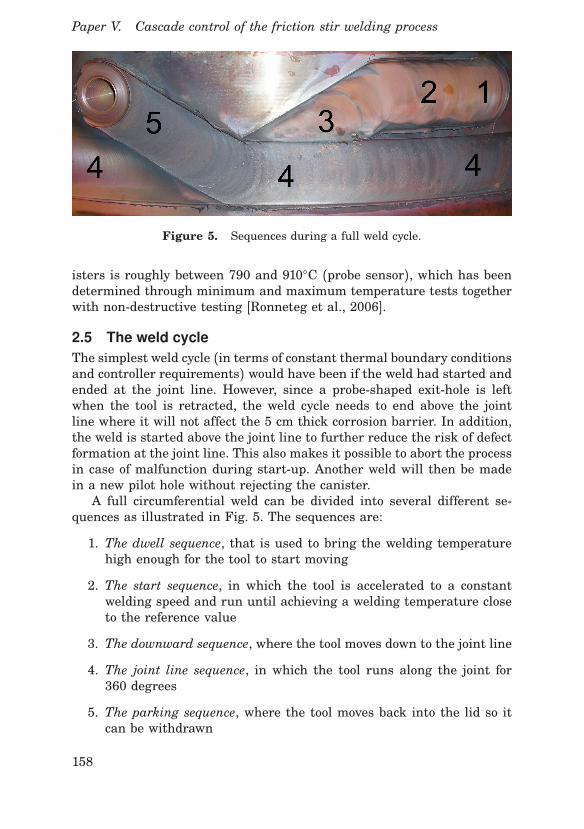
Paper V. Cascade control of the friction stir welding process
Figure 5. Sequences during a full weld cycle.
isters is roughly between 790 and 910○C (probe sensor), which has beendetermined through minimum and maximum temperature tests togetherwith non-destructive testing [Ronneteg et al., 2006].
2.5 The weld cycle
The simplest weld cycle (in terms of constant thermal boundary conditionsand controller requirements) would have been if the weld had started andended at the joint line. However, since a probe-shaped exit-hole is leftwhen the tool is retracted, the weld cycle needs to end above the jointline where it will not affect the 5 cm thick corrosion barrier. In addition,the weld is started above the joint line to further reduce the risk of defectformation at the joint line. This also makes it possible to abort the processin case of malfunction during start-up. Another weld will then be madein a new pilot hole without rejecting the canister.A full circumferential weld can be divided into several different se-
quences as illustrated in Fig. 5. The sequences are:
1. The dwell sequence, that is used to bring the welding temperaturehigh enough for the tool to start moving
2. The start sequence, in which the tool is accelerated to a constantwelding speed and run until achieving a welding temperature closeto the reference value
3. The downward sequence, where the tool moves down to the joint line
4. The joint line sequence, in which the tool runs along the joint for360 degrees
5. The parking sequence, where the tool moves back into the lid so itcan be withdrawn
158

2 Process description
Figure 6. Varying power input requirements for multiple circumferen-tial welds, using manual control. The different sequences are indicated byvertical lines and numbers in parentheses.
These will be indicated by a number from 1–5, in parenthesis, every timea sequence is referred to. This includes some of the plots.The different sequences in a weld cycle results in non-uniform thermal
boundary conditions throughout the weld. As a consequence, the powerinput requirement to keep the welding temperature within the processwindow varies throughout the 45 minute long weld cycle (see Fig. 6).
2.6 Known process disturbances
During a full weld cycle, there are three types of disturbances typically en-countered. Two of these can be directly related to the temperature signal,while the third is spotted in the torque measurements. These disturbances(including the variable thermal boundary conditions due to the path ofthe weld cycle) motivates why closed-loop control of the process is needed.Temperature disturbances The first type of temperature disturbanceis associated with the tool moving to or from areas that have been sig-nificantly heated already. During, e.g., the dwell sequence (1) the tem-perature increases while the tool still have not started moving. This willmainly affect the immediate area around the tool which is later left be-hind when the tool starts moving. Such disturbances are also encounteredduring the joint line sequence (4) as the tool constantly moves towards
159

Paper V. Cascade control of the friction stir welding process
a warmer area after approximately half the cycle. Due to the relativelyslow welding speed (86 mm/min), this kind of disturbance is rather lowfrequent in nature. Figure 6 shows how the power input varies during 5full weld cycles in order to keep a constant probe temperature. Note espe-cially how the mentioned temperature disturbance requires the power todrop (in order to keep a constant temperature) from around 200 degreesaround the lid and forward. In addition to this, the power input require-ment profile will vary from weld cycle to weld cycle according to the samefigure. Reasons for these variations can be; different properties in themanufactured components (tubes and lids), wear in spindle gear and/orreplaced spindle (necessary several times during a production period of40+ years). As a result, it is not advisable to control towards a presetpower input requirement for every weld cycle like the early proposed reg-ulator [Cederqvist et al., 2009], but to have an adjustable power inputrequirement.The second type of temperature disturbance occurs during the down-
ward and parking sequences (3 and 5) and is caused by greater heatconduction at the joint line compared to the lid. A consequence of thisis that the power input will have to increase by a fair amount duringthe downward sequence (3). Similarly, during the parking sequence (5),the power input will have to drop instead. Together with the first type oftemperature disturbance, this explains why the power inputs will need todrop rather fast at the end of the welds in Fig. 6 (360 degrees and on-wards). Even though these conduction disturbances are rather slow, theywill still have quite an impact on the temperature profile. The main rea-son is that they are relatively large in magnitude. The results of this willbe described thoroughly in Section 5.3.
Torque disturbances The torque required by the spindle to maintainthe tool rotation rate will vary depending on the properties of the ma-terial. The tool is, e.g., more likely to penetrate a bit deeper into thecopper in areas that have been significantly preheated, thus resulting ina higher torque value. The slightly different characteristics of the tubeand lid will also give rise to such torque variations that will primarily af-fect the power input, but secondarily also the welding temperature. Whilethese disturbances appear in all five sequences, it is only during the jointline sequence (4) that they are relatively insignificant. Figure 7 showsan abrupt torque disturbance that takes place during the downward se-quence (3) (occurs at time t = 127 seconds in the figure, which is 13seconds before the joint line sequence (4) starts). If such a disturbance isnot compensated for, by changing the tool rotation rate, the power inputwill drop by approximately 8%, causing the probe temperature to changein the order of −40○C. While this particular disturbance is both faster and
160

3 Controlling the FSW process
Figure 7. Torque disturbance during the downward sequence (3). Thetool depth signal confirms that the torque disturbance is not related to asudden change in the tool position.
of larger magnitude than most torque variations, it still gives a hint ofwhat one can expect will happen occasionally during production. Consid-ering that 1 degree in Fig. 6 corresponds to 6 seconds, it is also evidenthow much faster these disturbances are compared to their temperaturecounterparts. In Section 5.3, Fig. 18, it is shown how well this particulardisturbance was handled by the current controller (in terms of power andtemperature changes).
3. Controlling the FSW process
3.1 Background on FSW control
As of today, most friction stir welds are made on plates with more uniformthermal boundary conditions than cylinders (as well as other complex ge-ometries), and in aluminum, that has a relatively large process window,compared to steel, nickel and titanium alloys. For these reasons, thereare currently only a small (although growing) amount of FSW applica-tions using temperature control. The welding temperature is, for instance,rarely even measured. Instead, a welding operator might just decrease ax-
161

Paper V. Cascade control of the friction stir welding process
ial force if the tool depth increases as the tool and plate get hotter at theend of a long weld cycle.Robotic FSW applications face several challenges that the process de-
scribed in this article does not share; e.g. axial force control that is influ-enced by limited force capacity and deflection in the linkages and jointsof the robot (see e.g. [Soron, 2007]). [Longhurst et al., 2010], on the otherhand, use torque control to control tool depth instead of axial force con-trol. With this method, they also present an alternative way of controllingthe power input and thus also the temperature indirectly, although theaxial force remains uncontrolled.[Fehrenbacher et al., 2008] have approached closed-loop control of the
welding temperature through non-uniform boundary conditions (varyingbacking plate materials) by manipulation of the welding speed, and morerecently by adjusting tool rotation rate [Fehrenbacher et al., 2010]. A newstudy by [Mayfield and Sorensen, 2010] suggests development of a cas-caded control strategy similar to those presented by [Cederqvist et al.,2009] and in this article. [Wang et al., 2004] control the spindle torquewithin limited values by adjusting the depth of the tool into the weldedmaterial.Furthermore, the need for reliable control of the welding temperature
should increase as FSW is used on metals like titanium and steels thatwill have much smaller process windows. In addition, more complex ge-ometries of welding objects will result in non-uniform thermal boundaryconditions and thus also a need for welding temperature control.
3.2 Past and present control of the current process
While open-loop control may be a suitable solution for aluminum platewelding, it is just not sufficient for welding the copper canisters describedin this article. Such an approach would suffer from the many disturbancesoccurring during a full weld cycle, possibly bringing the welding temper-ature outside the process window. A series of 20 high quality welds of thecopper canisters have, however, already been produced thanks to manualchanges of the tool rotation rate by a skilled welding operator [Cederqvistand Öberg, 2007]. Still, to not be dependent on such an operator for 40+years of production, an automatic welding procedure needs to be devel-oped. A well-tuned controller will, in addition, react faster to disturbancesand be more reliable and repeatable than a welding operator.A previously used cascaded control strategy, controlling both towards
a fixed power input and temperature reference, was examined by [Ced-erqvist et al., 2009]. The current control strategy, presented in this arti-cle, has a clearer control design method as well as a better suited cascadestructure (further described in Sections 3.5 and 3.6).
162

3 Controlling the FSW process
3.3 Controller objectives
The main objective of the controller is to minimize the risk of the tem-perature ending up outside the process window. It is particularly crucialthat the probe does not break and, therefore, necessary to keep the probetemperature below 910○C. The temperature disturbances occurring dur-ing the downward sequence (3) will, however, generally make it easierto end up close to the lower limit of the window rather than the upper.During the parking sequence (5), the opposite will hold. Taking all theseobservations into consideration, it has been decided to generally use atemperature reference slightly below the middle of the process window.Another option would be to vary the set-point depending on the sequence.This is utilized during the parking sequence (5).To make sure that the controller can fulfill its main objective, it is
important that it can suppress disturbances in the spindle torque andtemperature efficiently. In addition, the controller should be able to re-spond quickly enough to reference tracking during the start-up and park-ing sequences (1–3 and 5) without experiencing any significant under orovershoots.
3.4 Choice of control- and measurement signals
A previous study by [Cederqvist et al., 2008] investigated the significanceof tool rotation rate, axial force and welding speed on the most importantoutput variable, the welding temperature (measured in the probe). It wasclear that changes in the tool rotation rate had the largest effect, whichmakes sense since it is directly proportional to heat and power inputs(defined in Section 2.2). Additionally, it was noted that power input hadbetter linear correlation with welding temperature than heat input. Asa direct result, changes in welding speed and/or axial force have beendeemed less useful to control the welding temperature and are, therefore,held constant. Changes in the tool rotation rate are instead used to controlthe welding temperature (and power input).[Cederqvist et al., 2009] proposed that the controller should use the
fastest responding tool temperature measurements, i.e. from the shoulderID sensor (see Fig. 4). This signal has a time delay of approximately 1second to disturbances in the power input, while the probe temperature,on the other hand, has about 5 seconds delay. From a control theoreticalperspective it is important to have as little dead time as possible in theprocess [Åström, 2000]. However, since the probe temperature measure-ments, to current knowledge, have the best correlation with regards toprobe fractures and wormhole defects [Cederqvist, 2011], it was decidedto let the controller use this signal rather than the less delayed ones. Inaddition, it has been found that the repeatability of the three tempera-
163
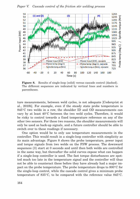
Paper V. Cascade control of the friction stir welding process
Figure 8. Results of single-loop (solid) versus cascade control (dashed).The different sequences are indicated by vertical lines and numbers inparentheses.
ture measurements, between weld cycles, is not adequate [Cederqvist etal., 2010b]. For example, even if the steady state probe temperature is845○C two welds in a row, the shoulder ID and OD measurements canvary by at least 40○C between the two weld cycles. Therefore, it wouldbe risky to control towards a fixed temperature reference on any of theother two sensors. For these two reasons, the shoulder measurements willonly be used as back-up signals, and a future controller should be able toswitch over to these readings if necessary.One option would be to only use temperature measurements in the
controller. This would result in a single-loop controller with simplicity asits main advantage. Figure 8 shows the probe temperature, power inputand torque signals from two welds on the FSW process. The downwardsequences (3) start at 0 seconds and until then both welds are controlledin the same way, but thereafter the solid curves expose what can happenif a single-loop controller is used. The fast torque disturbances are spot-ted much too late in the temperature signal and the controller will thusnot be able to counteract these before they have already had a major im-pact on the probe temperature. The probe temperature drops to 800○C forthe single-loop control, while the cascade control gives a minimum probetemperature of 835○C, to be compared with the reference value 845○C.
164

3 Controlling the FSW process
T
Figure 9. The proposed cascaded control structure.
The dotted curves, on the other hand, show the potential of using feed-back of the power input signal. The cascade controller used in this weldis the one presented in the next section. A possible challenge with theuse of a cascaded strategy is that the power input signal is rather noisy.If the controller design is made without taking this into consideration,one could risk ending up with a very high control signal variance, de-scribed by e.g. [Garpinger, 2009]. While an aggressive controller may giveoptimal performance, it could also result in unnecessary wear and tearon the equipment. Section 3.6 will include a deeper discussion on controltrade-offs.
3.5 Cascade control of the FSW process
A cascaded control strategy seems ideal for the characteristics of thisspecific FSW application with its fast, multiplicative, torque disturbancesand slower temperature counterparts. It has, therefore, been decided touse the controller structure displayed in Fig. 9. The process has beendivided into two subsystems. Process G1 holds the dynamics from thetool rotation rate (i.e. the control signal), u (rpm), to the power input,P (kW). This system will mainly hold the servo characteristics of thespindle motor. The outer process, G2, on the other hand, describes howthe power input is related to the probe temperature, T (○C). If needed,the measurements can be fed through low-pass filters, Cf1(s) and Cf2(s)respectively, for a less noise sensitive closed loop.The controllers C1 and C2 will be tuned in accordance with the control
objectives, such that disturbances are handled efficiently. One can assumethat the power input reference, Pr, will be low-frequent enough to not setany major challenges on the servo qualities of the inner loop. Set-pointtracking will thus mainly be an issue for the outer loop. In case the outer,load disturbance optimized, controller is not able to handle tracking wellenough, it will be handled separately through e.g. set-point filtering.
165

Paper V. Cascade control of the friction stir welding process
3.6 Controller design principle
The decision of how to best choose controllers C1 and C2 depends on thedynamics of G1 and G2. Since initial step response tests on the FSWprocess have shown that both processes have relatively simple dynamics(the final models are presented in Sections 5.1 and 5.2), the choice fellon either PI or PID controllers. These controllers also have the advan-tage that they are easier to tune and understand than more advancedalternatives. The tuning of the controllers will be very similar to that ofa newly presented method for design of robust PI- and PID-controllerswith constrained control signal activity [Garpinger, 2009]. The techniqueis based on optimization and built around a MATLAB® software tool, firstdescribed by [Garpinger and Hägglund, 2008]. The software uses a lineartransfer function model to find the PI or PID controller (either continuousor discrete time) minimizing the integrated absolute error (IAE)
IAE =∞∫
0
pe(t)pdt, (1)
during a unit step disturbance on the process input. The control error, e,is the difference between the controlled variable and its reference value.The IAE optimization guarantees stability and is constrained by H∞
robustness conditions
pSs(iω )p ≤ MS, pTs(iω )p ≤ MT , ∀ω ∈ R+, (2)
pSs(iω S)p = MS and/or pTs(iωT)p = MT , (3)
where Ss(s) and Ts(s) are the sensitivity function and the complementarysensitivity function respectively. The conditions stated in Eq. (3) force atleast one of the constraints to be active (in the frequency pointsω S and/orωT) and will, therefore, simplify the optimization. These constraints areknown to set closed-loop robustness towards process variations, distur-bances and non-linearities as described by for example [Åström and Häg-glund, 2005]. MS and MT are by default set to 1.4, known to give goodrobustness (e.g. phase margin 41.8○ and gain margin 3.5), but they canalso be changed by the user if desired.This PID design method is similar to some earlier presented methods
by [Panagopoulos et al., 2002], [Hägglund and Åström, 2004] and [Nord-feldt, 2005]. The biggest difference is the use of the fast software that isalso robust, easy to use and freely available on the web.The software can be used as described by [Garpinger, 2009] to limit
the control signal sensitivity to measurement noise by tuning of a low-pass filter acting on the measurement signal (like Cf1 and Cf2 do). This
166

4 Experimental setup
sensitivity is measured in terms of relative variance between the controlsignal and measurement noise
σ 2uσ 2n
≤ Vk. (4)
Vk is a user-specified upper limit on the maximum allowed gain of thecontrol signal variance, σ 2u, due to the measurement noise (with varianceσ 2n). The method suggests that the controller design is then a trade-offbetween maximum allowed wear on the equipment, robustness and controlperformance. If the equipment is sensitive, one will simply have to relyon a slower closed loop.
4. Experimental setup
4.1 Modeling and control design procedure
A significant part of the work behind this article was done to make surethat the procedure for process modeling and controller design are bothsimple and intuitive. The FSW process is expected to operate for morethan 40 years and it is likely to change during this time period. It is,therefore, wise to retune the controllers either when the FSW processhas known modifications or if the control starts to perform worse (e.g.determined through monitoring). A simple design method should enablepeople in the industry, without deep knowledge in automatic control the-ory, to carry out the steps needed to tune the controller if necessary. Clearinstructions and an intuitive strategy are also important for making surethat the necessary competence can be maintained within the company.
Modeling method and challenges Step response tests have been uti-lized for modeling the FSW process (i.e. determine G1 and G2). Two ad-vantages of the method are that it is fast and simple. Both are propertiesthat make it frequently used in the process industry today. A couple of itsdownsides are that it is disturbance sensitive and insufficient for iden-tification of higher order systems. But, the FSW process can most likelybe modeled well using only low-order models and it will also be modeledduring the joint line sequence (4), when disturbances are less significant.The FSW process is, however, also partly irreversible when using a
constant axial force. A somewhat simplified explanation of the behaviorwill be presented here. For example, if the weld metal gets colder it willresult in less tool depth and hence a lower power input. This will makethe weld even colder, and so forth. Similarly, if the process gets warmer itwill lead to a softer material, a greater tool depth and thus result in aneven hotter process. This theoretical behavior, sketched in Fig. 10 (dashed
167

Paper V. Cascade control of the friction stir welding process
Figure 10. Theoretical sketch of the process behaviors to open-loop(dashed) and closed-loop (solid) power input changes.
curves), makes it rather hard to use step response tests to determine amodel directly from tool rotation rate, u, to welding temperature, T . How-ever, since the power input responds much faster to changes in the toolrotation rate than the temperature, it is still possible to get around theseproblems by closing the inner loop. This way, it will be possible to do well-behaved step responses from power input reference, Pr, to temperature,T , similar to the solid curves in Fig. 10.
Controller design procedure The steps below follow the currently rec-ommended procedure for tuning of the controllers C1 and C2.
1. Do step response tests from u to P.
Make several steps of different magnitudes in both up- and downwarddirection to capture all relevant dynamics and possible non-linearities.
2. Find a linear model of G1.
Use any method available to estimate a model from step response data.See e.g. [Åström and Hägglund, 2005] for some possible methods.
3. Extract noise data from the power input signal.
Make sure there are no trends left in the resulting noise series.
168

4 Experimental setup
4. Design a robust PI or PID controller, C1 (possibly with a low-passfilter Cf1), for the inner loop.
Use e.g. the previously mentioned PID design tool to determine a robustcontroller, taking the trade-off between relative noise level, Vk, and per-formance, IAE, into consideration.
5. Close the inner loop and do step response tests from Pr to T .
Steps should be made in both up- and downward direction to reveal pos-sible non-linearities and differences in the dynamics.
6. Derive a linear model of G2 from the step response data.
Use the power input and temperature data to derive the model.
7. If relevant, get representative noise data from the temperature mea-surements.
Since the temperature measures contain very little noise, it could be thatthe noise throughput to Pr is so small that it literally drowns in the noiseof the power measurements. If not, the procedure will be the same as forstep 3.
8. Design a robust PI or PID controller, C2 (possibly with a low-passfilter Cf2), for the outer loop.
The design of C2 will be similar to the tuning of C1.While some of these steps are specific for the used PID design method,
the overall procedure is far from uncommon. Similar tuning schedulesfor cascade controllers are proposed by for instance [Forsman, 2005] and[Hägglund, 2008].
4.2 Performance test procedures on the FSW process
Once the two controllers have been derived, their performance will be tri-alled through two types of tests. The most common of these tests is thestart-up test, which normally run until about 60 seconds into the jointline sequence (4). The main reason why these tests are so common isthat the dwell, start and downward sequences (1–3) have shown to bethe most difficult to handle from a control perspective (see Section 2.6).Throughout the start and downward sequences (2 and 3), the temperaturedisturbances will act to increase the power input needed to maintain thetemperature at its set-point. These tests will determine how well the cas-cade controller acts to suppress the temperature reducing elements. Thedisturbances do, however, not come instantly once a new sequence hasbegun. So, while the controller should counteract temperature decreases,
169

Paper V. Cascade control of the friction stir welding process
Figure 11. Results of high power input during start-up. The differentsequences are indicated by vertical lines and numbers in parentheses.
it must not let the power input reach too high magnitudes before the startand downward sequences (2 and 3) begin. This is especially crucial justbefore the downward sequence (3) when the temperature is close to itsset-point. Figure 11 shows the results of a weld start-up where the powerinput got too high before the downward sequence (3), resulting in a tem-perature overshoot of 48○C. In an act to eliminate this unwanted feature,the power controller alone will be used before the downward sequence (3).The start-up is, therefore, currently handled according to the following 3steps:
1. Once the temperature reaches a first limit, the inner regulator startscontrolling towards a constant set-point, Pr.
2. A second temperature limit indicates when the tool should startmoving. At this moment, the power input reference, Pr, will start toincrease slowly along a linear slope.
3. The downward sequence (3) will start once a third temperature limithas been reached (typically about 10○C from its set-point, Tr). Thisis when the cascade controller is finally turned on.
Results showing the benefits of this new strategy are presented in Section5.3.
170
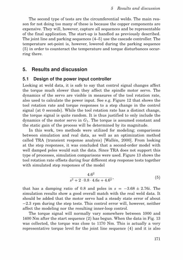
5 Results and discussion
The second type of tests are the circumferential welds. The main rea-son for not doing too many of these is because the copper components areexpensive. They will, however, capture all sequences and be representableof the final application. The start-up is handled as previously described.The joint line and parking sequences (4–5) use the cascade controller. Thetemperature set-point is, however, lowered during the parking sequence(5) in order to counteract the temperature and torque disturbances occur-ring there.
5. Results and discussion
5.1 Design of the power input controller
Looking at weld data, it is safe to say that control signal changes affectthe torque much slower than they affect the spindle motor servo. Thedynamics of the servo are visible in measures of the tool rotation rate,also used to calculate the power input. See e.g. Figure 12 that shows thetool rotation rate and torque responses to a step change in the controlsignal (at 0 seconds). While the tool rotation rate has a distinct change,the torque signal is quite random. It is thus justified to only include thedynamics of the motor servo in G1. The torque is assumed constant andthe static gain of the process will be determined by its magnitude.In this work, two methods were utilized for modeling; comparisons
between simulation and real data, as well as an optimization methodcalled TRA (transient response analysis) [Wallén, 2000]. From lookingat the step responses, it was concluded that a second-order model withwell damped poles would suit the data. Since TRA does not support thistype of processes, simulation comparisons were used. Figure 13 shows thetool rotation rate offsets during four different step response tests togetherwith simulated step responses of the model
4.62
s2 + 2 ⋅ 0.8 ⋅ 4.6s+ 4.62 , (5)
that has a damping ratio of 0.8 and poles in s = −3.68 ± 2.76i. Thesimulation results show a good overall match with the real weld data. Itshould be added that the motor servo had a steady state error of about−2.3 rpm during the step tests. This control error will, however, neitheraffect the modeling nor the resulting inner-loop control.The torque signal will normally vary somewhere between 1000 and
1400 Nm after the start sequence (2) has begun. When the data in Fig. 13was collected, the torque was close to 1170 Nm. This is actually a veryrepresentative torque level for the joint line sequence (4) and it is also
171

Paper V. Cascade control of the friction stir welding process
Figure 12. Changes in the tool rotation rate and torque signals to a stepchange in the control signal.
fairly in the middle of the interval stated above. The power input, P (kW),can be determined by
P = π
30000⋅ u ⋅ τ , (6)
where τ is the torque in (Nm) and u is the tool rotation rate in (rpm).Since the model (5) is described in u, a static gain of 0.12 seems suitablefor the process G1, such that the final model becomes
G1(s) = 0.12 ⋅4.62
s2 + 2 ⋅ 0.8 ⋅ 4.6s+ 4.62 . (7)
Due to the torque variations, however, the gain can vary between 0.105and 0.145.A time series of measurement noise data was then gathered by crop-
ping parts of the step responses and then piecing them back together afterapplying a linear detrending. This data could then be used in closed-loopsimulations to determine the Vk-value (see Eq. (4)) for each new controllerdesign.As described in section 4.1, it is a good idea to make the tuning as
easy as possible, as long as the controller objectives are met. Therefore,it makes sense to start out optimizing PI controllers, rather than PID,
172

5 Results and discussion
-0.5 0 0.5 1 1.5 2 2.5-10
-8
-6
-4
-2
0
Time (s)
Too
l rot
. rat
e of
fset
(rp
m) Experimental
Simulated
-0.5 0 0.5 1 1.5 2 2.50
5
10
15
20
Time (s)
-0.5 0 0.5 1 1.5 2 2.5
-20
-15
-10
-5
0
Time (s)
Too
l rot
. rat
e of
fset
(rp
m)
-0.5 0 0.5 1 1.5 2 2.5
0
5
10
15
20
Time (s)
Figure 13. Experimental (dashed) and model (solid) step responses inthe tool rotation rate during welding and simulation. The offsets were allclose to 400 rpm.
for the process. Using Garpinger’s MATLAB® tool on the process modelin Eq. (7) showed that tuning of a low-pass filter together with the PIcontroller had little effect on the relative noise throughput, Vk (previouslydefined in Section 3.6). As a way to still be able to set Vk, [Garpinger, 2009]has suggested that one can instead vary the robustness measures MS andMT . Therefore, 10 different PI controllers, with 10 different MS- and MT -values (from 1.015 to 1.35), were tuned using the design tool. Figure 14shows the trade-off curve between performance (IAE, previously definedin Section 3.6) and noise sensitivity (Vk) for these controllers. While afast controller results in good performance (low IAE-value), it will alsolead to a noise sensitive system (high Vk). A slower closed loop will, onthe other hand, give too bad performance. The key in the design is totry choosing a controller somewhere around where the curve bends themost. If the controller is made faster, one will not benefit that much inbetter performance compared to how much is lost in noise sensitivity. Ifthe closed loop is made slower, the noise sensitivity does not change much,
173

Paper V. Cascade control of the friction stir welding process
Figure 14. Performance and noise sensitivity trade-off curve for the in-ner control loop. The chosen controller is marked with a blue circle.
while the performance rapidly deteriorates. The controller
C1(s) = 1.07(
1+ 10.36s
)
, (8)
has an IAE-value of 0.34, a Vk-value of 3.15 (marked with a blue circlein Fig. 14) and MS = MT = 1.065 (very good robustness). It is thusclose to where the trade-off curve bends the most at the same time asthe proportional gain is close to 1. The latter argument suggests that thecontroller will prevent unnecessary amplification of quick changes in themeasurement noise. The inner closed loop has a bandwidth of 0.37 rad/s.In the end, it was decided to use this PI controller over a PID. While a
PID regulator may result in slightly better performance, it is not justifiedto add the extra complexity here. In section 5.3 it will be evident whythe inner loop does not need to be tuned any faster. It is fast enough forhandling the torque disturbances.Furthermore, it should be pointed out that the static gain variations
in G1 will have little effect on the power control since the closed-looprobustness is as good as it is. Also note that all controllers derived in thisarticle had to be discretized in order to implement them. This was doneusing the forward Euler method on the integral part, with a samplingtime of h = 0.1 s. All experiments presented here were thus carried outusing this sampling time.
174

5 Results and discussion
5.2 Tuning the temperature controller
Activating the inner-loop control, it is possible to do step response testsfrom power input reference, Pr, to probe temperature, T . Several stepchanges, of different magnitudes, were carried out in the vicinity of mul-tiple temperatures (from 815 to 845○C). Looking at the data, the processdynamics seem to vary a bit, possibly both with temperature and directionof the step. The reason why the process is direction dependent is becausethe control signal can only actively influence the heating of the process.For practical reasons, all step response tests have been made during thejoint line sequence (4). So, while it is useful to know how the process dy-namics depend on temperature, it is more important to know the modelaround the temperature reference, Tr. Figure 15 shows responses to apower input step in upward direction (at 0 seconds) that was made closeto the temperature set-point. Running the step response data throughTRA gave the following process model
G2(s) =11.6
(7s+ 1)2 e−5s. (9)
The simulated model output is marked as a dashed blue curve in Fig. 15.Controller design on the model showed that it gives good robustness andalmost unchanged performance for all process models derived (i.e. theones modeled at different temperatures and in downward direction too).Note that G2 is both of order two and has a rather significant time
delay. These characteristics could possibly be explained by the fact that theprobe temperature sensor is situated inside the tool. Therefore, the toolhas to be warmed up before the sensor can react to changes in the weldingtemperature. The reason why the probe sensor has a larger delay thanthe other two sensors is because the probe material has a lower thermalconductivity than the shoulder material, and the shoulder thermocouplesare placed closer to the weld metal.It was decided to use PI control for the outer loop as well. As will
be shown in the next section, it is quite enough for achieving the controlobjectives. For FSW applications with narrower process windows, however,a PID controller may be useful in the outer loop.The probe temperature measures hardly contain any noise at all. There
is, therefore, no reason to take the noise sensitivity into account whendesigning C2. Especially after choosing a PI controller to do the job. Thelow-pass filter is thus also left out. The trade-off between robustness andperformance will instead be the important part of the outer control-loopdesign.Two controllers were tuned using the PID design software, one with
175

Paper V. Cascade control of the friction stir welding process
Figure 15. Step test (at 0 seconds) from power input reference to probetemperature. A model simulation gives the dashed, blue, curve.
MS = MT = 1.4 and the other with MS = MT = 1.8. The first controller
C2(s) = 0.033 ⋅
(
1+ 111.2s
)
, (10)
is used during the joint line sequence (4) and gives a closed-loop band-width of 0.064 rad/s. The second, more aggressive, controller
C2(s) = 0.065 ⋅
(
1+ 114.0s
)
, (11)
is active during the downward and parking sequences (3 and 5) and re-sults in a closed-loop bandwidth of 0.14 rad/s. The reason for using a fastercontroller at those stages is because of the temperature disturbances ac-tive there (described in Section 2.6).
5.3 Performance experiment results
Start-up tests Figure 16 shows four weld start-ups (probe temperaturesin (a), power inputs in (b)) with the downward sequences (3) starting at0 seconds. These were produced using open-loop (dwell sequence (1)) andcascade control (start, downward and joint line sequences (2–4)) of thetemperature, similar to the weld in Fig. 11. The temperature reference
176

5 Results and discussion
Figure 16. Four old weld start-ups showing bad repeatability in probetemperature (a) and power input (b). The different sequences are indicatedby vertical lines and numbers in parentheses.
was set to 840○C. As one can see, this gave very bad repeatability betweenthe welds, with a power input that varied between 44 and 50 kW beforethe downward sequence (3) had even started. As a result, the probe tem-perature dropped below 800○C during one downward sequence (3) whileanother had a peak temperature above 890○C. While this is within thelimits of the process window, it is still a bit too close to really be on thesafe side.Making the changes to the control switches described in Section 4.2,
four new start-up tests were run and these are presented in Fig. 17 (probetemperatures in (a), power inputs in (b)). The power input control (be-fore 0 seconds) clearly makes the first three sequences more repeatable,producing welds that are within a satisfactory interval of 830 to 850○C.
177

Paper V. Cascade control of the friction stir welding process
Figure 17. Four new start-up tests using an improved control strategy,thus giving better repeatability in probe temperature (a) and power input(b). The different sequences are indicated by vertical lines and numbersin parentheses.
178

5 Results and discussion
Figure 18. Torque disturbance rejection during the downward sequence(3).
The temperature reference was set to 845○C in these tests. The temper-ature disturbances acting on the process are also visible in the figure.At 0 seconds, all welds have approximately the same power input andtemperature. Even though this temperature is close to the set-point, thepower input has to be increased considerably for the process to achievesteady-state during the joint line sequence (4). The temperature curvesalso tend to drop a bit after the downward sequence (3) has started. Theseare typical results of the temperature disturbances acting on the process.The fact that a more aggressive controller is used during the downwardsequence (3) will, however, reduce the temperature drop a bit.The large amount of torque disturbances occurring during the start-up
tests are good for showing how well the inner controller works. Figure 18displays the process data during the same disturbance that was shown inFig. 7. Although the power input instantaneously drops from 51 to 45.5kW, the controller increases the tool rotation rate by 20 rpm in the next 2seconds such that the power input is back at 50 kW. While the shoulder IDand OD signals have small bumps due to the disturbance, no significantprobe temperature deviations can be registered. This supports the claimthat the current inner PI controller is fast enough for the FSW process.
Circumferential welds Two sets of four circumferential welds were runusing the cascade controller strategy. The temperature reference was setto 840 and 845○C respectively. Figure 19 (a) shows how the temperaturesvaried during the joint line sequences (4), which can be compared to
179

Paper V. Cascade control of the friction stir welding process
Figure 19. Probe temperatures at the joint line using the cascade con-troller (a) compared to using manual control (b). A * refers to values onthe right y-axis.
20 circumferential welds (with a temperature reference of 850○C) thatwere made, in air (not argon), by a skilled welding operator in 2004 (seeFig. 19 (b)). It can be seen that there have been vast improvements sincethe argon gas and cascade controller were introduced.Figure 20 shows the parking sequences (5) for two of the first four
welds. In the first weld (ID 353), the temperature reference was set toa constant value during this sequence. The results of this were that allthree temperature measurements showed rather large increases, due tothe two temperature disturbances that are active during this sequence(see Section 2.6). To avoid the risk of ending up with a probe fracture,the temperature reference was manipulated to reduce this effect. Thesame figure shows that this change, although a bit primitive, is enoughto keep the probe temperature at a safe level. The shoulder OD signalwent up a bit even though the probe temperature decreased. This effectwas, however, much smaller than during the first weld.
6. Conclusions
The results presented in this article have shown that a combination ofa cascaded control structure and individual PI controllers is successfulin controlling the FSW process to seal copper canisters. While this isquite a specific process, the authors still believe that the methods andideas behind the results can be put into a wider context such that otherFSW applications can benefit from them too. In particular, applicationsthat have either varying thermal boundary conditions or narrow processwindows. Apart from this, any process that can be divided into two sepa-rate processes with distinctly different time constants will likely benefita great deal from a cascade controller.
180

6 Conclusions
Figure 20. Two parking sequences (5). t is here an abbreviation fortemperature.
Apart from the cascade structure, good process knowledge and a con-trol strategy adapted to the changing weld sequences have probably beenthe biggest contributors behind the satisfactory control of this application.The choice of the individual controllers has, however, not been as crucial.PI controllers in both loops have shown to be more than enough for han-dling the three types of disturbances as well as the reference tracking.This also fits well with the ambition of developing a simple procedure forcontroller design, such that people without a major education in controltheory can carry out the steps necessary.
Acknowledgments
The authors would like to thank the Swedish Nuclear Fuel and WasteManagement Company (SKB) for their financial support to this project.Thanks also to the ESAB personnel for their many visits to update theresearch possibilities of the welding equipment including controller im-plementation.
181
Paper V. Cascade control of the friction stir welding process
References
Åström, K. J. (2000). “Limitations on Control System Performance”. Eu-ropean Journal of Control 6:1, pp. 2–20.
Åström, K. J. and T. Hägglund (2005). Advanced PID Control. ISA – TheInstrumentation, Systems, and Automation Society, Research TrianglePark, NC.
Cederqvist, L. and T. Öberg (2007). “Reliability study of friction stirwelded copper canisters containing Sweden’s nuclear waste”. Relia-bility Engineering & System Safety 93:10, pp. 1491–1499.
Cederqvist, L., C. D. Sorensen, A. P. Reynolds, and T. Öberg (2008). “Im-proved process stability during friction stir welding of 5 cm thick cop-per canisters through shoulder geometry and parameter studies”. Sci-ence and Technology in Welding and Joining 46:2, pp. 178–184.
Cederqvist, L., R. Johansson, A. Robertsson, and G. Bolmsjö (2009).“Faster Temperature Response and Repeatable Power Input to aid Au-tomatic Control of Friction Stir Welded Copper Canisters”. In: FrictionStir Welding and Processing V. San Francisco, USA.
Cederqvist, L., A. P. Reynolds, C. D. Sorensen, and O. Garpinger (2010a).“Reliable sealing of copper canisters using new tool geometry and reg-ulator controlling tool temperature and power input”. In: 8th Interna-tional Friction Stir Welding Symposium. Timmendorfer Strand, Ger-many.
Cederqvist, L. (2011). Friction Stir Welding of Copper Canisters UsingPower and Temperature Control. PhD thesis. Department of MachineDesign, Lund University.
Cederqvist, L., O. Garpinger, T. Hägglund, and A. Robertsson (2010b).“Cascaded Control of Power Input and Welding Temperature DuringSealing of Spent Nuclear Fuel Canisters”. In: Proc. ASME DynamicSystems and Control Conference. Cambridge, Massachusetts.
Fehrenbacher, A., F. E. Pfefferkorn, M. R. Zinn, N. J. Ferrier, and N.A. Duffie (2008). “Closed-loop Control of Temperature in FrictionStir Welding”. In: 7th International Friction Stir Welding Symposium.Awaji Island, Japan.
Fehrenbacher, A., N. A. Duffie, N. J. Ferrier, M. R. Zinn, and F. E. Pf-efferkorn (2010). “Temperature measurement and closed-loop controlin friction stir welding”. In: 8th International Friction Stir WeldingSymposium. Timmendorfer Strand, Germany.
Forsman, K. (2005). Reglerteknik för processindustrin. Studentlitteratur,Lund, Sweden.
182
References
Garpinger, O. and T. Hägglund (2008). “A Software Tool for Robust PIDDesign”. In: 17th IFAC World Congress. Seoul, South Korea.
Garpinger, O. (2009). Design of Robust PID Controllers with ConstrainedControl Signal Activity. Licentiate Thesis ISRN LUTFD2/TFRT--3245--SE. Department of Automatic Control, Lund University, Swe-den.
Hägglund, T. (2008). Praktisk processreglering. Studentlitteratur, Malmö,Sweden.
Hägglund, T. and K. J. Åström (2004). “Revisiting the Ziegler-Nichols stepresponse method for PID control”. Journal of Process Control 14:6,pp. 635–650.
Larsson, P.-O. and T. Hägglund (2011). “Control Signal Constraints andFilter Order Selection for PI and PID Controllers”. In: 2011 AmericanControl Conference. San Francisco, California, USA.
Lohwasser, D. and Z. Chen, (Eds.) (2009). Friction Stir Welding: Frombasics to applications. Woodhead Publishing Ltd, 80 High Street, Cam-bridge CB22 3HJ, UK.
Longhurst, W. R., A. M. Strauss, G. E. Cook, and P. A. Fleming (2010).“Torque control of friction stir welding for manufacturing and automa-tion”. International Journal of Advanced Manufacturing Technology51:9, pp. 905–913.
Mayfield, D. W. and C. D. Sorensen (2010). “An improved temperaturecontrol algorithm for friction stir processing”. In: 8th InternationalFriction Stir Welding Symposium. Timmendorfer Strand, Germany.
Mishra, R. S. and M. W. Mahoney, (Eds.) (2007). Friction Stir Weldingand Processing. ASM International, Materials Park, Ohio 44073-0002.
Nandan, R., T. DebRoy, and H. K. D. H. Bhadeshia (2008). “Recent ad-vances in friction-stir welding – Process, weldment structure and prop-erties”. Progress in Materials Science 53:6, pp. 980–1023.
Nordfeldt, P. (2005). PID Control of TITO Systems. Licentiate ThesisISRN LUTFD2/TFRT--3238--SE. Department of Automatic Control,Lund University, Sweden.
Panagopoulos, H., K. J. Åström, and T. Hägglund (2002). “Design of PIDcontrollers based on constrained optimisation”. IEE Proceedings - Con-trol Theory & Applications 149:1, pp. 32–40.
Ronneteg, U., L. Cederqvist, H. Rydén, T. Öberg, and C. Müller (2006). Re-liability in sealing of canister for spent nuclear fuel. Tech. rep. SwedishNuclear Fuel and Waste Management Company.
Soron, M. (2007). Robot System for Flexible 3D Friction Stir Welding. PhDthesis. Department of Technology, Örebro University.
183

Paper V. Cascade control of the friction stir welding process
Thegerström, C. (2004). “Down to Earth and Below: Sweden’s Plans forNuclear Waste”. IAEA Bulletin 46:1, pp. 36–38.
Thomas, W. M., E. D. Nicholas, J. C. Needham, M. G. Murch, P. Temple-Smith, and C. J. Dawes (1991). Friction stir butt welding. InternationalPatent Application No. PCT/GB92/02203.
Upadhyay, P. and A. P. Reynolds (2010). “Effects of thermal boundaryconditions in friction stir welded AA7050-T7 sheets”.Materials Scienceand Engineering: A 527:6, pp. 1537–1543.
Wallén, A. (2000). Tools for Autonomous Process Control. PhD thesis ISRNLUTFD2/TFRT--1058--SE. Department of Automatic Control, LundInstitute of Technology, Sweden.
Wang, X. J., Z. K. Zhang, R. J. Guo, X. H. Han, and A. Rong (2004).“Application of MCGS for process control and realtime detection inthe process of Friction Stir Welding”. In: 8th International Conferenceon Control, Automation, Robotics and Vision. Kumming, China.
184

Supplement to Paper V
This supplement has been added to the thesis since Paper V uses the oldcontroller design procedure from [Garpinger, 2009]. Here we will showthat the newly proposed PID design method from Paper IV gives evenbetter control of the FSW process.Notice that all references made in this supplement are collected within
the reference list of Paper V.
S.1 Inner-loop control design
The inner-loop noise sensitivity and performance trade-off shown in Pa-per V, Fig. 14, was derived for PI controllers and with respect to variouslevels of robustness. This can be compared to the procedure proposed inPaper IV, which suggests that a given robustness is used to derive a setof controllers with respect to different filter time constants and integralgains.Since the sampling time of the FSW process, h = 0.1 seconds, is rather
long for the power input control, a discrete-time version of SWORD wasused to derive the inner-loop controllers in Paper V. Since the article waswritten, this tool has been updated to only use backward Euler consis-tently for the discrete-time controller approximations. This gives a slightimprovement in both closed-loop robustness and performance. Figure S.1shows the performance and noise sensitivity trade-off curves using boththe procedure from Paper IV (solid line) and Paper V (dashed line). PIDcontrollers are indicated by blue color, PI controllers by green and I con-trollers by red. The PI and PID controllers in the solid curve were derivedusing Ms = Mt = 1.4. Real noise data from the FSW process was usedin closed-loop Simulink® simulations, in order to derive the noise sensi-tivities, here given by the by the standard deviation of the control signal.The PI controller chosen in Paper V, Eq. (8), is indicated by a black circlein the figure. Notice that it lies slightly above the dashed trade-off curve
185

Supplement to Paper V
0 1 2 3 4 5 60
0.1
0.2
0.3
0.4
0.5IAE
σu [rpm]Figure S.1 Performance and noise sensitivity trade-off curves for the in-ner loop, with respect to control signal standard deviation. The solid lineshows the proposed set of PID (blue), PI (green) and I (red) controllers,while the dashed green line shows the previously proposed set of PI con-trollers. The formerly used PI controller is marked with a black circle andthe newly chosen controller is marked with a black square.
since it uses the old discrete-time version of SWORD. A new and moreaggressive I controller,
C1(s) =10s, (S.1)
marked with a black square in the figure, was chosen for the inner loop.This controller has considerably better performance than the old one, butthe noise sensitivity is also greater. However, we get a different pictureif we instead plot the trade-off curves with respect to a noise sensitivitygiven by the total variation (TV, Eq. (3.11) in the introductory chapters)per second, see Fig. S.2. Here, we see that there is a considerable dif-ference in the two trade-off curves, and the unfiltered PI controllers givea much higher noise sensitivity than the filtered controllers do. In fact,the old controller leads to a higher TV than the new one, even though ithad a much lower standard deviation. This result agrees well with those
186

S.2 Outer-loop control design
0 10 20 30 40 500
0.1
0.2
0.3
0.4
0.5IAE
TV per second [rpm/s]
Figure S.2 Performance and noise sensitivity trade-off curves for theinner loop, with respect to the total variation per second of the controlsignal. The solid line shows the proposed set of PID (blue), PI (green)and I (red) controllers, while the dashed green line shows the previouslyproposed set of PI controllers. The formerly used PI controller is markedwith a black circle and the newly chosen controller is marked with a blacksquare.
from [Larsson and Hägglund, 2011], which suggested to use a measure-ment noise filter of the least order that gives a high frequency roll-off.From Fig. S.2 it now makes even more sense to pick the best perform-ing I controller (S.1). Performance quickly deteriorates for lower integralgains at the same time as the TV does not decrease much. The relativeperformance gain in using PI control is also low in comparison to what itcosts in terms of noise sensitivity.
S.2 Outer-loop control design
The outer temperature control loop is much slower than the inner powerinput loop. Continuous-time and discrete-time PID control design will
187

Supplement to Paper V
0 0.1 0.2 0.3 0.4 0.5155
160
165
170
175
180
185
190
195
200IAE
σu [kW]Figure S.3 Performance and noise sensitivity trade-off curve for theouter temperature loop, with respect to control signal standard deviationdue to noise. The solid blue line shows the proposed set of PID controllers.The selected controller is marked with a black square.
thus lead to more or less the same controller, and we have chosen to usethe continuous-time version of SWORD.The temperature measurements contain relatively little noise, and it
should thus be fine to use an outer PID controller, rather than a PI con-troller as suggested in Paper V. A ten second sequence of temperaturenoise data was used to derive a performance and noise sensitivity trade-off curve for PID controllers with Ms = Mt = 1.4, see Fig. S.3. Controlsignal noise responses with several of these controllers were plotted toget visual feedback of their behavior. Two of them, with filter time con-stants T f = 0.2 and T f = 1.0, are shown in Fig. S.4. The blue curvesshow the outer-loop control signal, and the red curves show the resultinginner-loop control signal. Given this information, we choose the filter withT f = 1.0, which results in slow and relatively low magnitude variationsof the tool rotation rate, even though the performance loss is significant
188

S.2 Outer-loop control design
0 2 4 6 8 10-1
-0.5
0
0.5
1
0 2 4 6 8 10-1
-0.5
0
0.5
1
Time (s)
Magnitude
T f = 0.2
Time (s)
T f = 1.0
Figure S.4 Simulated control signal noise responses using real temper-ature noise data from the FSW process. Red signals show the inner-loopcontrol signal (rpm) and the blue signals show the outer-loop control sig-nal (kW). The responses to the left correspond to a low-pass filter withT f = 0.2, while the right hand plot shows the same with T f = 1.0.
in comparison to controllers with σu ( 0.1. This controller,
C2(s)Cf2(s) = 0.071(
1+ 110.55s
+ 5.13s)
⋅1
0.5s2 + s+ 1, (S.2)
gives IAE = 184.4, i.e. 16% worse performance than the best possible PIDcontroller,
C2(s) = 0.081(
1+ 110.26s
+ 4.8s)
.
The FSW process is especially sensitive to high power input valuesduring start-up, see Section 5.3 in Paper V. It is thus important that thefinal cascade controller does not give significant temperature overshootsduring the first weld sequences. Closed-loop reference step responses weresimulated on the system in Fig. 9, Paper V, using the PID controller fromEq. (S.2). Even if both the proportional and derivative set-point weightsare set to zero (i.e. b = c = 0, see Eqs. (1.8) and (1.10) in the introductorychapters), the simulations still show an 11% temperature overshoot. Sincethere are no other options for set-point weighting on the FSW process, wechoose to instead manipulate the overshoot using the Mt-value. ChoosingMt = 1.002 and T f = 1.0 in SWORD gives the PID controller and low-passfilter,
C2(s)Cf2(s) = 0.071(
1+ 112.63s
+ 4.63s)
⋅1
0.5s2 + s+ 1, (S.3)
189

Supplement to Paper V
0 50 100 150 200 250 3000
2
4
6
8
10
12
14
16
18
Temperature(○C)
Time (s)Figure S.5 Step set-point and load disturbance responses using outerPID controllers designed with Ms = Mt = 1.4 (blue) and Ms = 1.4, Mt =1.002 (red).
which results in the red reference and load disturbance responses shownin Fig. S.5. These can be compared to the responses in blue, given withthe previous controller (S.2). The overshoot has been decreased 3.2% atthe same time as the load disturbance IAE is just 2.8% worse. The PIDcontroller (S.3) was finally chosen to the control the FSW process togetherwith the I controller in (S.1).For comparison, the old PI controllers from Paper V have 79% (Ms =
Mt = 1.4) and 17% (Ms = Mt = 1.8) worse IAE than (S.3). The bestpossible, unfiltered, PI and I controllers with Ms = Mt = 1.4 give 58%and 189% worse performance respectively.
S.3 Results on the FSW process
So far, all plots have shown simulated data. But the improved cascadecontroller has also been tested on full welds. Probe temperatures of twofull welds during the joint line sequences are shown in Fig. S.6. The blue
190

S.4 Conclusions
0 500 1000 1500 2000838
840
842
844
846
848
850
852Temperature(○C)
Time (s)
Figure S.6 Probe temperatures during 60 seconds of the joint line se-quences of two full welds on the FSW process. The blue line shows the weldusing the old cascade controller from Paper V, while the red line shows theweld using the proposed cascade controller.
curve indicates a weld made with the two old PI controllers, and the redcurve shows the result with the new cascade controller. The temperaturereference was set to 845○C in both cases. The old cascade controller resultsin an IAE that is 58% higher than that of the new controller, i.e. fairlyclose to the previously predicted value of 79%. An example of the controlsignals from the two welds is plotted in Fig. S.7, showing 60 seconds ofweld data. As expected, the control signal of the new controller is slightlysmoother than the old one. This agrees with the prediction from SectionS.1.
S.4 Conclusions
It has been shown that the overall performance of the FSW temperaturecontrol can be significantly improved by using the new controller designmethod. We could probably have improved the cascade control even further
191

Supplement to Paper V
0 10 20 30 40 50 60415
420
425
430
435
Time (s)
Toolrotationrate(rpm)
Figure S.7 Tool rotation rate during part of the joint line sequences fromtwo full welds. The blue line corresponds to the old cascade controller fromPaper V and the red line to the proposed controller.
by using more realistic disturbance profiles in the SWORD software. But,this supplement was rather made to show how well the general optimalPID design method presented in Paper IV would work on the FSW process.
192