Analysis and Design Development ofParallel3-D Mesh ... · Analysis and Design Development ofParallel3-D Mesh Refinement Algorithms for Finite Element Electromagnetics with Tetrahedra

Analysis and Design Development ofParallel3-D Mesh

Refinement Algorithms for

Finite Element Electromagnetics with Tetrahedra

by

Da Qi Ren, B.Eng., M.A.Sc.

A thesis submitted to the Faculty of Graduate Studies and Research in partial fulfillment

of the requirements for the degree of Doctor ofPhilosophy.

Computational Analysis and Design Laboratory

Department of Electrical and Computer Engineering

McGill University

Montréal, Canada

September 2006

©Da Qi Ren 2006

1+1 Library and Archives Canada

Bibliothèque et Archives Canada

Published Heritage Branch

Direction du Patrimoine de l'édition

395 Wellington Street Ottawa ON K1A ON4 Canada

395, rue Wellington Ottawa ON K1A ON4 Canada

NOTICE: The author has granted a nonexclusive license allowing Library and Archives Canada to reproduce, publish, archive, preserve, conserve, communicate to the public by telecommunication or on the Internet, loan, distribute and sell th es es worldwide, for commercial or noncommercial purposes, in microform, paper, electronic and/or any other formats.

The author retains copyright ownership and moral rights in this thesis. Neither the thesis nor substantial extracts from it may be printed or otherwise reproduced without the author's permission.

ln compliance with the Canadian Privacy Act some supporting forms may have been removed from this thesis.

While these forms may be included in the document page count, their removal does not represent any loss of content from the thesis.

• •• Canada

AVIS:

Your file Votre référence ISBN: 978-0-494-32234-5 Our file Notre référence ISBN: 978-0-494-32234-5

L'auteur a accordé une licence non exclusive permettant à la Bibliothèque et Archives Canada de reproduire, publier, archiver, sauvegarder, conserver, transmettre au public par télécommunication ou par l'Internet, prêter, distribuer et vendre des thèses partout dans le monde, à des fins commerciales ou autres, sur support microforme, papier, électronique et/ou autres formats.

L'auteur conserve la propriété du droit d'auteur et des droits moraux qui protège cette thèse. Ni la thèse ni des extraits substantiels de celle-ci ne doivent être imprimés ou autrement reproduits sans son autorisation.

Conformément à la loi canadienne sur la protection de la vie privée, quelques formulaires secondaires ont été enlevés de cette thèse.

Bien que ces formulaires aient inclus dans la pagination, il n'y aura aucun contenu manquant.

ABSTRACT

Optimal partitioning of three-dimensional (3-D) mesh applications necessitates

dynamically determining and optimizing for the most time-inhibiting factors, such as load

imbalance and communication volume. One challenge is to create an analytical model

where the programmer can focus on optimizing load imbalance or communication

volume to reduce execution time. Another challenge is the best individual performance of

a specific mesh refinement demands precise study and the selection of the suitable

computation strategy. Very-Iarge-scale finite element method (FEM) applications require

sophisticated capabilities for using the undedying parallel computer' s resources in the

most efficient way. Thus, c1assifying these requirements in a manner that conforms to

the programmer is crucial.

This thesis contributes a simulation-based approach for the algorithm analysis and

design of parallel, 3-D FEM mesh refinement that utilizes Petri Nets (PN) as the

modeling and simulation tool. PN models are implemented based on detailed software

prototypes and system architectures, which imitate the behaviour of the parallel meshing

process. Subsequently, estimates for performance measures are derived from discrete

event simulations. New communication strategies are contributed in the thesis for parallel

mesh refinement that pipeline the computation and communication time by means of the

workload prediction approach and task breaking point approach. To examine the

performance of these new designs, PN models are created for modeling and simulating

1

each of them and their efficiencies are justified by the simulation results. Aiso based on

the PN modeling approach, the performance of a Random Polling Dynamic Load

Balancing protocol has been examined. Finally, the PN models are validated by a MPI

benchmarking pro gram running on the real multiprocessor system. The advantages of

new pipelined communication designs as weU as the benefits of PN approach for

evaluating and developing high performance paraUel mesh refinement algorithms are

demonstrated.

ii

SOMMAIRE

Pour partitionner des applications de maillage tridimensionnel (3-D) de façon

optimale, il faut déterminer et optimiser dynamiquement les facteurs qui ralentissent le

plus le processus, comme le déséquilibre de charge et le volume de communication. Un

des défis les plus difficiles à relever consiste à créer un modèle analytique dans lequel le

programmeur puisse se concentrer sur l'optimisation du déséquilibre de charge et du

volume de communication afin de réduire le temps d'exécution. Autre défi: pour que la

décomposition d'un maillage spécifique se traduise par une excellente performance

individuelle, il est impératif d'étudier et de choisir soigneusement la stratégie

informatique la mieux adaptée. Les applications FEM (Méthode des éléments finis) à très

grande échelle nécessitent des fonctionnalités sophistiquées pour pouvoir exploiter le plus

efficacement possible les ressources parallèles sous-jacentes d'un ordinateur. Par

conséquent, il est essentiel de classer ces spécifications de façon à faciliter au maximum

le travail du programmeur.

Cette thèse propose une approche fondée sur la simulation pour l'analyse

algorithmique et la conception d'une méthode de décomposition de maillage 3-D FEM

utilisant les réseaux de Petri (RdP) comme outil de modélisation et de simulation. Les

modèles RdP mis en œuvre reposent sur des architectures système et des prototypes

logiciels détaillés, qui reproduisent le comportement du processus de maillage parallèle.

Par la suite, les estimations effectuées pour les mesures de la performance sont dérivées

iii

de simulations par événements discrets. Cette thèse présente de nouvelles stratégies de

communication pour la décomposition de maillage parallèle qui canalisent le temps de

communication et de calcul informatique via deux approches: l'une repose sur la

prédiction de la charge de travail, l'autre sur le point de rupture de processus. Pour étudier

la performance de ces nouvelles stratégies, nous avons procédé à leur modélisation et à

leur simulation par le biais de modèles RdP créés à cet effet. Les résultats de la

simulation prouvent l'efficacité de ces modèles. Nous avons étudié la performance du

protocole équilibrage de charge dynamique. En dernier lieu, les modèles RdP ont été

validés par un programme MPI de conduite de tests de performance

benchmarking tournant sur le véritable système multiprocesseur. Nous démontrons ainsi

les atouts de ces nouvelles méthodes de communication ainsi que les avantages d'une

approche utilisant les RdP pour évaluer et développer des algorithmes de décomposition

de maillage parallèle hautement performants.

iv

ACKNOWLEDGMENTS

1 would like to express my Slllcere gratitude to my supervIsor Dr. Dennis D.

Giannacopoulos for the invaluable suggestions, inspiration, guidance, insightful

discussions, encouragement and support throughout these past four years. He showed

constant attention and care about my research, personal needs and future career

development. 1 would like to thank Dr. J. S. McFee for the discussion and suggestions. 1

would also like to thank Dr. J. S McFee and Dr. Zilic Zeljko for their care, support and

helpfulness in my research work. 1 am also grateful to Drs. Dennis Giannacopoulos,

Milica Popovic, J. P. Webb and D. A. Lowther, for the use of the hardware and research

software in the CAD labo

Most of aU, 1 thank my parents for their kindness and support. 1 also thank my brother

and my sister for their help.

v

TABLE OF CONTENTS

TABLE OF CONTENTS ................................................................................................ vi

LIST OF TABLES ........................................................................................................... x

LIST OF FIGURES ........................................................................................................ xi

PREFACE ......................................................................................................................... 1

Conceming the Format of This Thesis ........................................................................ .1

Contributions of Authors .............................................................................................. 2

CHAPTER 1: Introduction ............................................................................................... 4

1.1 Mesh Refinement in Finite Element Method ......................................................... .4

1.2 Statement of Problem .............................................................................................. 5

1.3 Challenges of Algorithm Design Development in the Scope of the Thesis ........... 9

1.4 Motivation ............................................................................................................. 1 0

1.5 Thesis Objectives .................................................................................................. 11

1.6 Claim of Originality .............................................................................................. 13

1.7 Overview of the Thesis ......................................................................................... 14

CHAPTER 2: Literature Review .................................................................................... 15

2.1 Problem Formulation and Component Issues of the Thesis ................................ .15

2.2 Modeling and Simulation for Performance Prediction in Parallel Algorithm

Design ......................................................................................................................... 16

2.3 Modeling and Simulation Tools Design ............................................................... 21

vi

2.4 Petri Nets ............................................................................................................... 23

2.5 Dynamic Load Balancing for Structured Adaptive Mesh Refinement.. ............... 26

2.6 Inter-Proeessor Communication in ParaUel Mesh Refinement ........................... .28

CHAPTER 3: A Preliminary Approach to Simulate ParaUel Mesh Refinement

with Petri Nets for 3-D Finite Element Electromagneties .............................................. 32

3.1 Introduction ........................................................................................................... 32

3.2 Geometrie Mesh Refinement Model.. ................................................................... 34

3.3 ParaUel Algorithm Analysis .................................................................................. 36

3.4 ParaUel Meshing Environments ............................................................................ 38

3.5 Modeling ofComponents ..................................................................................... 40

3.6 Simulation Results ................................................................................................ 43

3.7 Conclusion and Future Work ............................................................................... .44

CHAPTER 4: Analysis and Design ofParaUel3-D Mesh Refinement Dynamic

Load Balaneing Algorithms for Finite Element Eleetromagnetics with Tetrahedra ..... .47

4.1 Introduction ........................................................................................................... 48

4.2 Geometrie Mesh Refinement Model. .................................................................... 50

4.3 RP-DLB ParaUel Mesh Refinement Model .......................................................... 51

4.4 Results ................................................................................................................... 59

4.5 Conclusion ............................................................................................................ 62

CHAPTER 5: ParaUel Mesh Refinement for 3-D Finite Element Electromagnetics

with Tetrahedra: Strategies for Optimizing System Communication ............................. 64

5.1 Introduction ........................................................................................................... 65

5.2 ParaUel Mesh Refinement Approach .................................................................... 66

vii

5.3 Communication Model ......................................................................................... 68

5.4 Pipelined Communication Design ........................................................................ 70

5.5 Petri Nets Model and Simulation .......................................................................... 72

5.6 Results ................................................................................................................... 75

5.7 Conclusion ............................................................................................................ 79

CHAPTER 6: Efficient Pipelined Communication Design for Parallel Mesh

Refinement in 3-D Finite Element Electromagnetics with Tetrahedra ........................... 81

6.1 Introduction ........................................................................................................... 82

6.2 Parallel Hierarchical Tetrahedra and Octahedra Subdivision ............................... 83

6.3 Communication Model ......................................................................................... 85

6.4 Pipelined Communication Design ........................................................................ 88

6.5 Petri Nets Model and Simulation .......................................................................... 90

6.6 Results ................................................................................................................... 93

6.7 Conclusion ............................................................................................................ 95

CHAPTER 7: Parallel Hierarchical Tetrahedral-Octahedral Subdivision Mesh

Refinement: Performance Modeling, Simulation and Validation ................................... 99

7.1 Introduction ......................................................................................................... 100

7.2 Parallel HTO Subdivision ................................................................................... 102

7.3 Modeling with Petri Nets .................................................................................... 104

7.4 MPI Benchmark .................................................................................................. 109

7.5 Results ................................................................................................................. 109

7.6 Conclusion .......................................................................................................... 112

CHAPTER 8: Conclusion ............................................................................................. 114

viii

8.1 Summary and Discussion .................................................................................... 114

8.2 Future Work ........................................................................................................ 116

REFERENCES ............................................................................................................. 117

ix

LIST OF TABLES

Table 3.1: The sub-domain partitioning ......................................................................... 37

Table 3.2: Theoretical timing estimations ..................................................................... 38

Table 3.3: Simulation results for 1, 3, 4 and 6 CPUs in a Mater-Slave model. ............. 42

Table 3.4: Comparison ofload imbalance ..................................................................... 42

Table 5.1: Workload Assignment: ................................................................................. 73

Table 5.2: Number of Elements: .................................................................................... 74

x

LIST OF FIGURES

Figure 2.1: Components of the research ......................................................................... 15

Figure 3.1: Subdivision of a tetrahedron for mesh refinement. ...................................... 35

Figure 3.2: Octahedron subdivision ................................................................................ 35

Figure 3.3: The adjacent surface between each element after subdivision .................... .35

Figure 3.4: ParaUel mesh refinement environment. ........................................................ 39

Figure 3.5: Petri Nets model of a processor assigned to a sub-domain ......................... .41

Figure 3.6: Petri Nets model for master processor in 6 CPU system ............................ .41

Figure 3.7: Number of geometric entities vs. execution time ......................................... 44

Figure 4.1: Mesh refinement model: (a) tetrahedron subdivision; (b) primary

octahedron subdivision; (c) secondary octahedron subdivision ................... 51

Figure 4.2: Conceptual outline ofparallel mesh refinement with RP-DLB. .................. 52

Figure 4.3: Discrete events chart for a slave PE ............................................................. 53

Figure 4.4: Timing diagram for proof of (4.7) ................................................................ 55

Figure 4.5: Framework for mesh refinement Petri Nets model. ..................................... 56

Figure 4.6: Petri Nets Module: (a) RP-DLB task sub-division; (b) tetrahedron

and octahedron sub-division ......................................................................... 58

Figure 4.7: The OveraU structure ofPN model for paraUel mesh refinement in a

6 PE system. (a)Workload Reassigning; (b) Polling Process. (Note:

this is a complete version of the original figure in the paper.) ..................... 60

xi

Figure 4.8: RP-DLB performance results: (a) speedup vs. number of elements

for different numbers of PEs; (b) parallel efficiency vs. number of

PEso ............................................................................................................... 61



Figure 5.2: Parallel mesh refinement approach .............................................................. 67

Figure 5.3: Timing for parallel mesh refinement in typical master-slave model.. .......... 70

Figure 5.4: Timing for pipelined communication design ............................................... 72

Figure 5.5: Petri-Nets parallel communication model for 6 PEso ................................... 74

Figure 5.6: Petri Nets module for pipelined communication of Pk and Pj .............. 75

Figure 5.7: Performance results (without designed pipeline):

(a)communication cost; (b) load imbalance ............................................... 77

Figure 5.8: Performance results (with designed pipeline): (a) communication

cost; (b) load imbalance ................................................................................ 78



Figure 6.2: Parallel mesh refinement approach ............................................................. 87

Figure 6.3: Timing for parallel mesh refinement in typical master-slaves design .......... 88

Figure 6.4: Timing for parallel mesh refinement of pipelined communication

design ............................................................................................................ 90

Figure 6.5: Sub-domain decomposition ofrectangular resonant cavity ......................... 91

Figure 6.6: PN parallel communication model for 8 PEso .............................................. 92

xii

Figure 6.7: Parallel Speedup: (A) non-pipelined communication, (B) with

pipelined communication ............................................................................. 94

Figure 6.8: Pipeline Speedup: Pipeline vs. non-pipelined communication .................... 95


octahedron subdivision; (c) secondary octahedron subdivision ................. 103

Figure 7.2: Parallel mesh refinement approach ........................................................... .104

Figure 7.3: Timing for parallel mesh refinement in master-slaves mode!. ................... 106

Figure 7.4: The PN Co-Module: tetrahedron and octahedron sub-division .................. 107

Figure 7.5: The PN model for parallel mesh refinement with six PEso ........................ 108

Figure 7.6: Validation results for mesh computation processes .................................. .111

Figure 7.7: Validation results for data formatting processes ....................................... .111

Figure 7.8 : Validation results for data gathering processes .......................................... 112

xiii

PREFACE

Concerning the Format of This Thesis

This thesis is prepared in the form of five self-contained research papers designated

Chapters 3-7.

Chapter 3 entitled "A preliminary Approach to Simulate ParaUel Mesh Refinement

with Petri Nets for 3-D Finite Element Electromagnetics" appears in the refereed

conference proceedings of the 10th International Symposium on Antenna Technology

and Applied Electromagnetics (ANTEM 2004).

Chapter 4 entitled "Analysis and Design of paraUel 3-D Mesh Refinement Dynamic

Load Balancing Aigorithms for Finite Element Electromagnetics with Tetrahedra" and

Chapter 5 entitled "ParaUel Mesh Refinement for 3-D Finite Element Electromagnetic

with Tetrahedra: Strategies for Optimizing System Communication" are published in the

IEEE Transactions on Magnetics, Volume 42, Issue 4, Pages 1235-1238 and pages 1251-

1254, respectively.

Chapter 6 entitled "Efficient Pipelined Communicaiton Design for ParaUel Mesh

Refinement in 3-D Finite Element Electromagnetics with Tetrahedra" and Chapter 7

1

entitled "Parallel Hierarchical Tetrahedral-Octahedral Subdivision Mesh Refinement:

Performance Modeling, Simulation and Validation" are submitted to the IEEE

Transactions on Magnetics.

The five papers are organized into a cohesive dissertation with the addition of three

chapters and five connecting pages: Chapter 1 serves as an introduction to the thesis,

Chapter 2 gives a comprehensive literature review, and Chapter 8 provides the discussion

and conclusion. The short linking pages are also included to provide logical bridges

between the different papers, one of each conjunction of two papers.

Contributions of Authors

The applicant, Da Qi Ren is the primary author of chapters 1-3, 5-8, and the second

author of chapter 4 of which Prof. Dennis D. Giannacopoulos is the primary author.

Prof. Dennis Giannacopoulos initiated the research, and contributed ideas, suggestions,

guidance, challenges, inspirations, insightful discussions, manuscript editing, support and

other invaluable supervision through out the thesis. The design, execution, interpretation

and reporting of the research were primarily performed by the applicant Da Qi Ren.

Prof. Steve McFee is the co-author of chapter 7 and 8 who contributed suggestions,

insightful discussions and manuscript editing.

2

Chulhoon Park and Baruyr Mirican are co-authors of chapter 8. They contributed the

MPI co ding work.

3

CHAPTER 1: Introduction

1.1 Mesh Retinement in Finite Element Method

The finite element method (FEM) is a powerful numerical technique for the

approximate solution of continuum electromagnetic problems [1]. The FEM requires the

discretization of the spatial domain with finite elements: for two dimensional problem

triangles and rectangles, in three dimensions tetrahedral and hexahedral elements are

commonly used. Aiso a mixture of different types of elements is possible, but after the

evaluation of various other implementations and for simplicity, tetrahedral discretization

is the most popular to be applied in solving the electromagnetic problems.

The resolution of the finite element mesh, i.e. the maximum size of the finite elements,

is determined by the smallest features in the solution of the goveming partial difference

equations. These features need to be properly resolved, and the approximation of the

exact solution by the test functions has to be sufficiently accurate to give meaningful

results. In order to reduce the size of the initial finite element mesh so as to make it fine

enough to resolve the details of the geometrical model, global or partial mesh refinement

can be do ne at mn time. This makes the mesh geometry in the input data files much

smaller. Moreover, convergence of the results will usually be checked with a refined

4

finite element mesh. Thus, the creation of the geometrical model and its mesh refinement

are very demanding tasks, which require sophisticated tools [2][3].

An ideal mesh generation and refinement method can lead to optimal complexity and

give the most accurate results with the smallest numerical computational effort. High

performance mesh refinement algorithm development is a very active research are a,

which is significant in many FEM applications such as numerical electromagnetics.

1.2 Statement of Problem

Determining accurate 3-D finite element solutions for very-large-scale problems in

electromagnetics can be highly challenging and computationally expensive. A number of

the component procedures and stages involved in the FEM solution process can be

accelerated with parallel processing. 3-D mesh refinement is one of them, because

modem FEM applications can require extremely large numbers of elements.

There are two basic issues to consider in parallel 3-D mesh refinement. The first is

data parallelism: i.e. exploiting the concurrency in the mesh refinement by subdividing

the complete space into sub-domains. The second is function parallelism and distributed

shared memory management: i.e. exploiting parallelism inherent in the algorithm itself,

including the load balancing, inter-processor communication etc. In data parallelism, an

existing method to handle the complexities of full 3-D mesh refinement is geometry

decomposition. This takes apart the topological features of the upper level domain into

5

sub-domains, refines meshes in each sub-domain, and then reassembles the sub-domains

to create a comprehensive model for the complete space [4]. Function parallelism

manages the mapping of logical shared address space and the locating and accessing of a

needed data item among processing elements (PEs), and facilitates an efficient

communication scheme in a parallel or shared memory system. Most approaches handle

this by utilizing sorne kind of distributed shared memory management and inter processor

communication method.

Complexities of load balancing and inter-processor communications are two of the

crucial challenges in developing high performance parallel mesh refinement software. In

a parallel program the problem is initially split up into parts and assigned to each

processor in the parallel system. In order to achieve the maximum parallel speedup,

every processor working for the parallel pro gram should be busy all the time, otherwise

delays and idle time will reduce the overall performance. For a heterogeneous

environment composed of different speeds and capabilities processors, the numerical

problem has to be distributed following an approach that makes all processors complete

their assignment at the same time, thus no one has to wait for others to synchronize their

results. [5] Dynamic load balancing (DLB) schemes are taken into consideration to

efficiently utilize the computing resources provided by distributed systems. The

underlying DLB algorithm methods insert and remove finite elements and modify the

number of unknowns at run time, thus, the computational effort will increase for

processors working on a partition of the finite element mesh where elements have been

inserted, and decrease for those where elements have been removed. These operations

6

will disturb the initial load balancing and require a new partitioning of the finite element

mesh, redistribution of the current data to the processors and re-initialization, before the

calculation can be resumed [6]. The partitions generated by load balancing algorithms

should be optimized with the following goals in mind: first to balance the workload on

every level; second to maintain data locality; third to minimize inter-processor

communication; and fourth to minimize number and optimize the size of patches. A patch

is a piece of space in a sub-domain that is to be relocated by the load balancing algorithm.

On the other hand, research in inter-processor communication (IPC) on parallel and

distributed memory multiprocessors involves the investigation of efficient routing and

collective communication algorithms relative to different kinds of networks. IPC has

generally been implemented using shared memory, local networks, seriaI communication

links or first in first out ports [7]. The performance of shared memory systems is limited

by the multiprocessor bus bandwidth. As processors are added to the system, message

traffic may overload the bus and performance may degrade. In cases where bus

bandwidth is not a limiting factor, shared memory systems offer the advantage that

globally accessible data is directly available for every task. In general, the performance

requirements inc1ude high throughput, low latency and low overhead. To analyze a

parallel algorithm' determining the number of computational steps, estimating

communication overhead and transmission speed are integral. In a message passing

system, the time required to send any message must be considered in the overall

execution time of a problem. The parallel execution time is composed of two parts: a

computation part and a communication part. The computation time can be estimated in a

7

similar way to that of a sequential algorithm. In the case when more than one process is

being executed simultaneously, the computation time is the steps of the most complex

process. In the analysis of the computation time it is usually assumed that aIl the

processors are identical and operating at the same speed. This is suitable for a specially

designed multiprocessor, but may not be the case for workstation clusters because one of

the powerful features of such clusters is that the computers need not be the same. Taking

into account heterogeneous computers would be difficult in a mathematical analysis,

which is why the use of identical computers is assumed. Different types of computers are

taken into account by choosing implementation methods that balance the computational

load across the available computers. The communication time depends upon the size of

the message, the underlying interconnection structure, and the mode of data transfer [8].

The high performance IPe for parallel mesh refinement requires maintaining data locality

and communication in the synchronization phase when adjacent patches are not in the

same partition. The efficient inter-processor communication strategy does the following:

first it minimizes inter-processor data transmission latency; second it minimizes the

number of patches; third it adjusts the size of patches for cache optimizations; and fourth

it minimizes data movements while re-balancing [9].

Due to the computational complexity of paraUe1 mesh refinement systems, the

parallelisation of real applications is a complex and time consuming task. Even with

powerful multiprocessors and distributed systems, the performance of paraUe1 FEM mesh

refinement is highly dependent on the efficiency of programming paradigms and the

architecture of parallel computing systems. In the development of a parallel mesh

8

refinement system the programmer must consider both the results generated by the

pro gram under development and the behaviour of the parallel pro gram in order to obtain

the best possible performance.

1.3 Challenges of Algorithm Design Development in the Scope of the Thesis

The main challenge is to create an analytical model where the programmer can focus

on optimizing load imbalance or communication volume to reduce execution time in

parallel 3-D mesh refinement. A desired model helps the programmer select and

configure the optimal mesh configuration, simulation and computer characteristics.

Individual suitability needs to be considered. No single partitioning scheme performs

best for all types of parallel mesh refinement applications and systems. For a given

application, the most suitable partitioning technique depends on input parameters and the

application's run-time state [10]. This necessitates adaptive run-time management,

inc1uding the use of application runtime state to select and configure the best partitioning

strategy.

Another challenge arises from large-scale parallel mesh refinement applications, such

as meshing implementations which produce up to 109 elements. Parallel mesh refinement

applications place different requirements on the partitioning strategy to enable efficient

use of computer resources. Significantly improving the scalability of large-scale mesh

refinement requires sophisticated capabilities for using the resources of the underlying

9

parallel computer in the most efficient way. A way of classifying these requirements in a

way that conforms to the programmer is crucial.

Parallel mesh refinement methods offer the potential for more efficient accurate FEM

solutions in electromagnetics, however, its parallel implementation presents many

challenges in dynamic resource allocation, data-distribution, load-balancing, and run-time

management. The implementation efficiency of parallel mesh refinement applications is

limited by the computational capacity, parallel infrastructure, load balance,

communication and synchronization overheads minimization.

Finally, validating the performance predictions of the model by comparing them with

actual measurements from real computation is another challenge. The results must show

that the proposed model generally captures the inherent optimization needs in parallel

mesh refinement applications. To conclude that a model is making a useful contribution,

tracking and adapting to the behaviour of the model optimization should potentially lead

to a decrease in execution times.

1.4 Motivation

The primary motivation for this research is to explore performance prediction facility

in the development of parallel mesh refinement, with the focus on the usability of

simulation tools for reducing the user effort in the parallel programming cycle. Based on

the prediction facility, the programmer can pro vide a synthetic skeleton of the parallel

10

meshing application, including sorne parameters that characterise it. This skeleton can be

used as input to the simulator and the performance prediction analysis can be done before

completely developing the application. Therefore, the information obtained is related to

an application that has not been completely developed and this fact saves the time and

effort of the programmer.

A secondary motivation is to investigate the improvement of the scalability of large

scale mesh refinement from the underlying simulation model, and to explore the

dependency between the computation performance and the number of processing

elements in the computer resource.

The final motivation is to explore efficient communication strategies to reduce latency

for paraUel 3-D finite element mesh refinement in electromagnetics.

1.5 Thesis Objectives

The goal is to investigate effective modeling and simulation technologies for the

performance and computational complexity prediction in the design development and

optimization of three-dimensional (3-D), paraUel mesh refinement. It is also to design

and test new pipelined communication strategies for minimizing the inter-processor

communication costs in this mesh refinement. The outcome from this analysis will help

paraUel program developers determine which options provide the best performance. In

detail, the objectives are described as follows.

11

The first objective is to model and simulate the performance of parallel Hierarchical

Tetrahedral-Octahedral (HTO) Subdivision mesh refinement by Petri Nets, and provide

the paraUel speedup results with increasing number of elements. The second objective is

to sample and translate to latency characteristics in the simulation model from the given

application parameters such as the grid hierarchy and the number of processors; and

system parameters such as CPU speed and communication bandwidth. Thirdly, to model

and simulate the performance of the Random Polling Dynamic Load Balancing (DLB) in

parallel HTO mesh refinement, and examine the results by comparing them with the

performance of parallel HTO mesh refinement without DLB. The fourth objective is to

develop efficient communication strategies for improving the parallel inter-processor

communication performance. The finally objective is to conduct an experimental

evaluation and validation of this PN model, showing its effectiveness for accurately

capturing the dynamic behaviour of parallel mesh refinement applications. This will be

achieved using MPI benchmarks running on the real parallel computer.

The following research achievements are produced: first, the performance model and

simulation of parallel HTO mesh refinement by Petri Nets is created, and the speedup

results are measured; second, the system parameters are successfully abstracted and

verified through the model validation; third, the Random Polling Dynamic Load

Balancing is applied to parallel mesh refinement and the performance is examined by its

PN models; fourth, two pipelined communication strategies are designed, prediction

scheduling strategy and break point strategy. Finally, the performances of the two new

designs have been examined by PN models and the validation of the PN models are

12

successfully performed by MPI benchmarks. Note that, the tetrahedral elements

considered in this work are appropriate for use in both vector and nodal finite element

implementations.

1.6 Claim of Originality

This thesis, to the best of author' s knowledge, presents the following original

contributions:

• A methodology ofmodeling and simulating the performance ofparallel3-D mesh

refinement by using Petri Nets;

• A new pipelined communication design: prediction scheduling approach, and its

performance examination;

• A new pipelined communication design: break points approach, and the design's

performance examination;

• A performance study for the application of Random Polling Dynamic Load

Balancing on the parallel 3-D HTO mesh refinement and;

• Inception of concepts: Workload Prediction Pipelined Communication; Breaking

Points Pipelined Communication; Load Imbalance Ratio.

13

1. 7 Overview of the Thesis

Chapter 2 presents a comprehensive review of the literature conceming the existing

approach for performance prediction. It addresses the following themes: formaI modeling

and simulating techniques; the application of Petri Nets (PN); the design and

development of Dynamic Load Balancing (DLB); and inter-processor communication in

parallel mesh refinement. Chapter 3 introduces the preliminary approach to apply the PN

method in modeling and simulation of parallel 3-D mesh refinement. In Chapter 4 both

the application of PN method for the performance evaluation of a specifie DLB scheme

in 3-D parallel mesh refinement and the Random Polling Dynamic Load Balancing

Protocol are described. Chapter 5 presents a new pipelined communication design in

parallel mesh refinement, namely load prediction approaches, and examines its

performance with the PN method. Chapter 6 elaborates on another new pipelined

communication design for efficient inter-processor communication, namely, a breaking

point approach, and the efficiency of the design is also examined by the PN model. To

validate the PN method in developing high performance parallel mesh refinement

algorithms, the PN models and simulations in terms of MPI benchmark computation

results obtained from actual software implementation and experimental performance

measurement on the real parallel environment are compared and evaluated. The

validation results are provided in Chapter 7. Chapter 8 is a brief summary and conclusion,

and suggestions for future work.

14

CHAPTER 2: Literature Review

2.1 Problem Formulation and Component Issues of the Thesis

The structured contents of the research include the design, modeling, implementation

and evaluation ofparalle13-D mesh refinement, as shown in Figure 2.1.

Dcsign Dcvcloprncnt

Parallel Algoritluns in 3-D FEM Mesh Refmernent

! Dcsign Modcling - Validation Tirned Petri Nets

l Modeling J Simulation Expcrimcnts Vs.

Dcsign Simulation ExperirnentsJ Computing C J MPI Irt;'lernentation 1---

Tirned Petri Nets

l Output ofDcsign Analysis

Performance Results and Best Solution

Figure 2.1: Components of the research.

15

As part of this research, techniques for parallelization, task mapping and parallel

pipelined communications have been developed and deployed. Another important goal of

this project is to "develop a performance modeling tool in parallel FEM mesh refinement

optimization by using the Petri Nets approach. As shown in Figure 2.1, the work

involves: (1) the design model and design simulation by timed Petri Nets created for

examining and evaluating the performance of the new algorithm design; (2) experimental

evaluation of the new algorithm design by applying MPI benchmarks running on the real

parallel computer; (3) validation of the correctness of the PN models by checking the

simulation results with the computation results; (4) determining the best solution to a

specific problem by analyzing the results from PN modeling and performance simulation.

Other studies have shown significant efforts related to the work in each component of

the the sis shown in Figure 2.1. The literature review below is discussed and organized

thematically and methodologically.

2.2 Modeling and Simulation for Performance Prediction in Parallel Algorithm

Design

Performance prediction evaluates an algorithm with modeling and simulation tools in

the earlier design stage of software development to provide valuable information and

optimizations that will result in increased performance. Performance study requires an in

depth knowledge of the system being evaluated and a careful selection of the

performance evaluation technique depending on the intended goals of that study.

16

Converting a given performance problem to a form in which established performance

evaluation techniques are applicable and time constraints imposed by system designers

can be met constitutes an important part of the performance analyst art.

Simulation models can be categorized broadly as being probabilistic or deterministic.

Trace driven and execution-driven simulation belong to deterministic simulation. Among

situations where probabilistic models are more suitable, often a representation is given by

considering a collection or a family of random variables instead of a single one.

Collections of random variables indexed by a parameter such as time and space are

known as stochastic processes. CUITent performance prediction techniques are

investigated in the literature review and sorne typical simulation modeling techniques and

architectures developed by research institutes and technology companies are summarized.

A traditional modeling and simulation technique is using benchmarking and cyc1e

accurate simulators to enable quantitative modeling of performance for high performance

computing applications. Performance Modeling and Characterization (PMac) developed

by the San Diego Supercomputer Center [11] characterizes influential factors affecting

performance by measuring each in isolation, and then integrating these factors to arrive at

models predictive of performance. PMac is built upon three distinct techniques: first, they

use machine profiles for the characterizations of the rates at which a machine can carry

out fundamental operations abstract from the particular application; second, the memory

access pattern signature for determining the loads and stores depending on the size of the

problem and access pattern; and third, the application signatures, i.e. the characterizations

17

of an application which independent of host machine, III detailed summaries of the

fundamental operations to be carried out.

Trace driven and execution-driven simulation are very popular in computer system

analysis due to their high credibility. In trace driven simulation, data parameters

previously measured from traces of memory references have been first collected, these

data are the input of system model that simulates the behavior of the computer system

under consideration. A trace is a time-ordered record of events of the system under

construction. Both trace-driven and execution-driven simulation belong to the class of

deterministic performance evaluation techniques because each simulation repetition

produces exactly the same results for the measures of interest and there is no randomness.

Integrated Software Infrastructure Centers (ISIC) in Scientific Discovery through

Advanced Computing created automated modeling tools that are able to characterize

large applications running at scale while simultaneously simulating the memory

hierarchies of multiple machines in parallel [12]. They ported the requisite tracer tools to

multiple platforms, added control-flow and data dependency analysis to the tracers used

in the performance tools. Also they used the modeling tools to develop performance

models for certain strategic codes and applied the modeling methodology to make a large

number of "blind" performance predictions on certain applications targeting the most

available system architectures at present. Researchers at the University of Califomia at

San Diego address the problem of modeling time-sensitive, dynamic and heterogeneous

performance information and using it to predict performance of distributed applications

in a meta computing environment [13]. This methodology involves the design and

18

development of structural models / performance grammars. Performance predictions

made by the system are generated from compositional models. Structural models consist

of components which represent the performance activities of the application. Each

component can be instantiated using time-dependent dynamic parameters at the level of

"accuracy" appropriate for its use. Quality of Information (Qoln) measures measure each

prediction generated by a processing element (PE). Qoln measures and values provide a

way of quantifying qualitative information so that it can be used to improve application

schedules and ultimately application performance.

In parallel stochastic processes, the knowledge of the behavior of the stochastic

process is highly desirable in understanding the real-life situation. Stochastic modeling is

a more high-Ievel abstraction of the system. The Chaos Project is the performance

prediction for large scale data intensive applications on large scale parallel machines at

the University of Maryland [14]. The Chaos project mainly focuses on performance

prediction for applications for existing and future parallel machines. The vast amount

data processed requires expensive hardware configurations and renders direct

experimentation on the target machine virtually impossible. Chaos developed a

simulation-based framework to predict the performance of data intensive applications for

it. The framework consists of two components: application emulators and a suite of

simulators. Application emulators accurately capture the behavior of data intensive

applications. The simulators model the IIO and communication subsystems of the parallel

machine at a level sufficient for accurately predicting application performance. They

introduced a new technique called loosely coupled simulation that abstracts the

19

processing structure as a simple dependency graph into the simulator while preserving the

application workload. The technique allows accurate and relatively inexpensive

performance prediction for very large scale parallel machines.

Analytical / numerical models and queumg theory are used to explore and solve

fundamental, theoretical problems in the analysis of application data, mathematical

models of system, workloads and performance. The IBM research group has focused on

the analysis of data from a wide range of systems to demonstrate complex arrivaI and

service patterns that include timing dependencies and non-stationary effects. The IBM

research group shows that these complexities can have a significant impact on

performance. These theoretical results may be further exploited to develop practical

solutions for performance problems in many different areas of research such as traffic

generation and benchmarking, model validation, workload and performance

forecasting [15].

A modem complex system is often composed of many interconnected components that

exhibit rich behaviors due to the complex system-wide interactions. Modeling these

systems leads to complex stochastic hybrid models that capture the large number of

operational and failure modes. The distributed and parallel systems group at the

University of Innsbruck separates the performance simulation into two parts: system level

prediction [16] and application level prediction [17]. In system level prediction, a

distributed system called "network weather service" is used to periodically monitor and

forecast the performance of the network and the computational resources. The

20

information can be delivered over a given time interval. Also they designed a Resource

Prediction System which is an extensible toolkit for designing, building, and evaluating

systems that predict the dynamic behavior of resources in distributed systems.

Application level prediction including the application behavior, data transfer predictions,

grid information, and run times use historical information. In detail, the hybrid approach

is implemented in two steps. (1) Modeling: employs the Unified Modeling Language

(UML) to model parallel and distributed applications. To provide an adequate tool

support they have developed Teuta, which is a graphical editor for UML. (2) Simulation:

a parameterized simulation tool was developed for cluster and grid architectures based on

the UML model of an application and a simulator for a target architecture in the building

blocks approach.

2.3 Modeling and Simulation Tools Design

This is a review of the design of modeling and simulation software in author' s scope

during the research work. A modeling and simulation tool is always required to

accurately demonstrate all aspects of parallel systems, especially sorne graphical based

software packages are used for model debugging, validation, and verification.

UML (Uniform Modeling Language) has been used to model the application and a

simulator for target paraUel architecture which can predict the execution behavior of the

application model on cluster and grid architectures. Researchers at the University of

21

Innsbruck developed the UML based modeling tool "The Performance Prophet" [18] for

high performance computing system modeling and simulation.

Based on the MPI and OpenMP paradigms, IBM High Performance Computing

Toolkit (HPCT) [19] is an integrated environment for performance analysis of sequential

and parallel applications. It provides a common framework for IBM's mid-range servers,

including pSeries and eSeries servers and Blue Gene systems, for both AIX and Linux.

They also have projects that aim to strengthen the HPCT toolkit and exp and to coyer

most aspects of performance analysis for high-performance computing, including CPU,

memory, communication and 1/0 profiling.

VHDL based simulation kemel has been implemented on top of general purpose time

warp simulation kemel, this combination provides paraUel VHDL simulation capability,

namely TyVIS. The TyVIS aUows user to simulate and execute VHDL codes that have

been translated into the TyVIS C++ intermediate form. The VHDL simulator provides

the functionality required by a VHDL simulation kemel as specified by the VHDL LRM

[20].

C-based simulation language is developed by the ParaUel Computing Laboratory at

UCLA, namely Parsec, for sequential and parallel execution of discrete-event simulation

models. It can also be used as a paraUel programming language. It is available in binary

form for academic institutions only [21] [22]. GloMoSim is a scalable simulation

environment for wireless and wired network systems. It employs the parallel discrete-

22

event simulation capability provided by Parsec. GloMoSim currently supports protocols

for a purely wireless network. If s anticipated that in the future it will be possible to

simulate a wired as weIl as a hybrid network with both wired and wireless capabilities.

GloMoSim and the binary code can be downloaded by academic institutions for research

purposes only. Commercial us ers must use QualNet, the commercial version of

GloMoSim [23].

Software Performance Engineering (SPE) techniques have the potential to reduce cost

and improve a systems' reliability. These techniques use performance models to provide

data for the quantitative assessment of the performance characteristics of software

systems as they are developed. SPE·ED is a tool designed specifically to support the SPE

methods and models defined in Connie U. Smith's book [24]. Using a small amount of

data about envisioned software processing, SPE·ED creates and solves performance

models, presenting visual results. It provides performance data for requirements and

design choices and facilitates the comparison of software and hardware alternatives for

solving performance problems.

2.4 Petri Nets

A Petri Net (PN) is a graphical and mathematical modeling tool which consists of

places, transitions, and arcs that conne ct them. The concept of Petri Nets has its origin in

Carl Petri's 1962 dissertation. Petri Nets are a promising tool for describing and studying

systems that are characterized as being concurrent, asynchronous, distributed, paraIlel,

23

deterministic, and stochastic. The development of high-Ievel Petri Nets in the late 70's

and hierarchical Petri Nets in the late 80's promoted Petri Nets with data concepts and

hierarchy concepts. Coloured Petri Nets (CPN) is one of the two most weU known

dialects of high level Petri Nets. CPN incorporates both data structuring and hierarchical

decomposition without compromising the qualities of the original Petri Nets. CPN

combine the strengths of ordinary Petri Nets with the strengths of a high-Ievel

programming language. Petri Nets provide the primitives for process interaction, while

the programming language provides the primitives for the definition of data types and the

manipulations of data values. A CPN model consists of a set of modules and each

contains a network of places, transitions and arcs. The modules interact with each other

through a set of well-defined interfaces, which is similar to many modem programming

languages. Another most weU known approach, Stochastic Petri Nets, were formaUy

developed in the field of computer science for modeling system performance. They

exponentiaUy distribute firing time which is attached to each transition. In Generalized

Stochastic Petri Nets (GSPN), transitions are aUowed to be either timed exponentiaUy

distributed firing time or immediate zero firing time. Immediate transitions always have

priority over timed transitions. GSPN analysis can be separated into four stages:

generating the extended graph which contains the markings of stochastic information

attached to the arcs so aU the markings are related to each other; eliminating the

vanishing markings with zero sojoum times and the corresponding transitions; analyzing

the steady state transient and cumulative behaviour; outputting the measures such as the

average number of tokens in each place and the throughput of each timed transition.

24

Petri Nets are popular in computer performance study and evaluations. There are

existing varieties of Petri Nets software developed for different purposes in system

modeling and simulation. We review sorne typical approaches in this chapter.

The work in [25] presents an experimental implementation of the asynchronous

decomposition method for the high level Petri net named Stochastic Well formed Nets

(SWN). The method combines multi-valued decision diagram methods for structured

Markov chains with the theoretical results for decomposable SWN. The implementation

allows computing performance indices for very large and very symmetric systems.

Jeremy T. Bradly [26] present an extended Continuous Stochastic Logic (eCSL) that

provides an expressive way to articulate performance queries at the Semi-Markov

Stochastic Petri Nets (SM-SPNs) model. SM-SPNs are a high level formalism for

defining semi-Markov processes. It supports queries involving steady-state, transient and

passage time measures. Computational Algorithm for Product-Form of Competing

Markov Chain [27] considers a particular class of stochastic Petri Nets exhibiting a

product form solution over sub-nets. The considered product form solution criterion is

based on a factorisation of the equilibrium distribution of the model in terms of

distributions of the continuous time Markov chains of the basic sub-models. They can

easily be adapted for other performance formalisms where the identification is considered

in [27]. There are different kinds of stochastic Petri Net-based modeling paradigms in

[28]: Generalized Stochastic Petri Nets (GSPNs), Deterministic and Stochastic Petri Nets

(DSPNs), and Fluid Stochastic Petri Nets (FSPNs). Marsan et al. modeled a wireless

internet access system via the global system for mobile (GSM) communications [29].

25

Their work shows that aIl three Petri Net-based paradigms considered provide very

similar performance predictions for sorne configurations of GSM/GPRS systems, and for

sorne of the performance metrics of interest. A timed hierarchical coloured Petri Nets

framework for modeling distributed computing environments is used in the web server

performance analysis [29]. Analysis of the performance of the web server model reveals

how the web server will respond to changes in the arrivaI rate of requests, and alternative

configurations of the web server model were examined.

In this thesis, Petri Nets is introduced for the modeling, analysis and design of

algorithms in parallel finite element mesh refinement. Petri Nets-based models allow for

a relatively detailed description of a system due to their formaI syntax and functional

semantics, and can reveal key characteristics of system performance stochastically. While

Petri Nets have been used for discrete event-based simulation of various applications, to

our best knowledge, they have not been considered previously for parallei 3-D mesh

refinement for finite element electromagnetics with tetrahedra. In addition, we use the

proposed approach for the design of a random polling (RP)-DLB algorithm and new

design of pipelined communication algorithms for a specific 3D parallei mesh refinement

model suitable for FEM electromagnetics with tetrahedra.

2.5 Dynamic Load Balancing for Structured Adaptive Mesh Retinement

Load balancing is an important performance issue in parallel algorithm design. It

intends to achieve the minimum execution time by spreading the tasks evenly across the

26

processors. Based on this, the redistribution of load among the processors during

execution time is performed in order to make each processor have the same or nearly the

same amount of work load. Dynamic load balancing (DLB) methods decide which

processor an idle processor should ask for more work, these methods can be divided into

two categories: (1) in the pool-based method (PBM), one control processor has all the

incomplete work, and an idle processor asks this fixed processor for more work. (2) In a

peer-based DLB method, aIl the work is initially distributed among different processors,

and an idle processor selects a peer processor as the work donor by using a DLB method

such as random polling, nearest neighbour, and global round robin (GRR) or

asynchronous (local) round robin (ARR). This thesis examines the performance of

random polling DLB in parallel HTO mesh refinement, and this review lists the CUITent

dynamic load balancing approaches for parallel3-D mesh refinement applications.

There are a number of infrastructures that support dynamic load balancing for parallel

and distributed implementations of a parallel mesh refinement application algorithm.

Pollack [33] proposed a scalable hierarchical approach that considers dynamic load

balancing in parallel and distributed systems, and implemented a system named Parallel

Load Balancer (PaLaBer) on the Intel Paragon XP/S. It uses multilevel control for

dynamic load balancing and for the communication manager. This hierarchical load

balancer uses both a non-pre-emptive and pre-emptive process migration to balance load

between the processors. PaLaBer targets overall scheduling and load-balancing of tasks

from multiple applications rather than dynamic load-balancing for adaptive applications

such as parallel mesh refinement.

27

Hierarchical Partitioning Aigorithms (HP A) partitions the computational domain into

sub-domains which assign each sub-domain to dynamically configure hierarchical

processor groups. Processor hierarchies and groups are formed to match natural

hierarchies in the grid structure [34]. This approach is more flexible and can be static or

adaptive, allowing the distribution to reflect the state of the adaptive grid hierarchy and

exploit it to reduce synchronization requirements, improve load-balance, and enable

concurrent communications and incremental redistribution.

In addition, there are adaptive computational and data-management engines for

parallel mesh refinement, such as: Paramesh [30], which adds adaptation to existing seriaI

structured grid computations; SAMRAI [31], which is an object-oriented framework for

implementing parallel structured adaptive mesh refinement simulations; and other

approaches such as AMROC [32].

2.6 Inter-Processor Communication in Parallel Mesh Refinement

The network connection and communication speed, and the communication patterns of

the parallel programs can critically affect the performance of the message passing

machines. In distributed-memory multi-computers, synchronization, data sharing and the

speed and efficiency of communication are very important for overall performance. The

general study of inter-processor communication is not covered in this review. The inter-

28

processor communication in parallel mesh refinement has its specific characteristics to be

investigated in this thesis.

Two important factors are the size of work transfer and the data arrangement. If

communication cost is negligible, the smallest possible piece of work may be transferred

for achieving best possible performance. In general, the size of work-transfer depends on

communication cost among other parameters. The data arrangement in parallel inter

processor communication between each adjunct do main is another important issue that

can affect the blocks in communication. This review provides in detail the inter-processor

communication schemes that are currently used in 3-D parallel meshing software.

To optimize inter-processor communication at the level of algorithm design, a typical

method is patch strategy. Patch strategy is an algorithm that supports solution at the

algorithm level description of data transfer [36]. It works as an interface to user-defined

coarsen 1 refine operations and boundary conditions. The phases of computation are

expressed using variables, and coarsen/refine operators that are independent of mesh

configuration. The communication schedule manages data transfers, and the algorithm

automatically treats complexity of different data types.

Sorne existing schemes in parallel mesh refinement software are developed to manage

data transfer between adjacent partitions. The approach is defined in the data packaging

level of the communication layers. Amortize cost [35] is one of the inter-processor

communication approaches for structured adaptive mesh refinement. It creates sending

29

and receiving sets over multiple communication cycles, data from various sources are

packed into single message stream. This approach supports complicated variable-Iength

data, one send per processor pair with low latency.

Another approach developed at the task level parallel implementation is given in [37].

It aims to reduce the re-gridding cost of parallel mesh generation for large-scale parallel

computers. The clustering algorithm is parallelized by packaging the SPMD (Single

Program Multiple Data) implementation as asynchronous, interruptible tasks. A task

manager selects active tasks to minimize communication wait times. This task parallel

implementation significantly Improves scaling trend over the synchronous

implementations. Clustering cost scales much better than output globalizing cost.

Different from the above inter-processor communication approaches, the goal of the

research in this thesis is to design new pipelined communication methods, and apply

the se new designs to the specific problem of hierarchical tetrahedral and octahedral

subdivision. Aiso the behaviour of the communication components in the new designs are

modeled, and their performances are simulated.

30

CHAPTER 3: A Preliminary Approach to Simulate

Parallel Mesh Refinement with Petri Nets for 3-D Finite

Element Electromagnetics

Preface

The following chapter is included as a paper published in the Conference Proceedings

of the 10th International Symposium on Antenna Technology and Applied

Electromagnetics (ANTEM 2004), pages 127-130, Ottawa, Canada, July 20-23,2004.

The paper's role is to introduce the Petri Nets methodology and the preliminary

application ofPN on modeling and simulating parallel3-D mesh refinement, specifically,

the Hierarchical Tetrahedral and Octahedral Sub-division mesh refinement algorithm.

Based on the PN model presented in this paper Random Polling Dynamic Load

Balancing protocol was examined in chapter 4 and the new design of pipelined

communication approaches were evaluated in chapters 5 and 6.

31

CHAPTER 3: A Preliminary Approach to Simulate Parallel Mesh

Refinement with Petri Nets for 3-D Finite Element Electromagnetics

Da Qi Ren and Dennis D. Giannacopoulos

Abstract:

An approach utilizing Petri Nets for modeling and evaluating parallel, unstructured

mesh refinement is developed. A model is implemented based on a detailed software

prototype and system architecture, which mimics the behavior of the parallel meshing.

Subsequently, estimates for performance measures are derived from discrete event

simulations. The potential benefits and related costs of this new approach for developing

high performance parallel mesh refinement algorithms are examined.

Key Words:

Finite Element Method, Performance Modeling, Parallel Mesh Generation, Petri Nets

3.1 Introduction


approximate solution of electromagnetic engineering problems. Due to the computational

32

complexity of three-dimensional (3-D), paraUe1, unstructured mesh generation for

modem applications, the performance of the method is highly dependent on the

efficiency of programming paradigms and the architecture of paraUe1 computing systems:

for example, the underlying algorithm; the inter-processor communication pattern; the

synchronization of tasks; etc. The goal of modeling paraUel computing systems is to

examine the specific paraUe1 system architecture and software techniques in advance, in

order to enhance the paraUe1 computing performance. The main advantage of this

approach is that the design and implementation of a paraUe1 mesh generator can,

potentiaUy, be optimized in order to achieve the best performance for a given cost among

different alternatives.

Today, several techniques are used for paraUe1 meshing performance analysis.

However, many of them are based on benchmarks, i.e., executing programs on known

environments. Unfortunately, these types of deterministic evaluation techniques are

inefficient for performance studies in the early design stages of a computer system. On

the other hand, Petri Nets mode1s can reveal the key characteristics of a system

stochasticaUy. Moreover, Petri Nets aUow for a relative1y detailed description of systems

due to their formaI syntax and functional semantics. In addition, algebraic reasoning,

deduction of properties and equational transformation preserving behavior are valuable

characteristics of Petri Nets. These properties have proven useful for the functional and

temporal specification of both software and hardware for paraUel and distributed systems.

33

3.2 Geometrie Mesh Refinement Model

The quality of finite element solutions depends on several factors including the size

and shape of the elements, the approximation properties of the underlying finite element

solution space, and the nature of the true solution to the problem under consideration. For

3-D electromagnetic analysis and design with the FEM, tetrahedra are often employed to

achieve the geometric discretization of the problem domain [38]. From a computational

viewpoint, tetrahedra possess several desirable modeling properties, such as the ability to

define complete polynomial interpolation functions throughout their volume. However,

one difficulty associated with employing tetrahedra, is the geometric complexity involved

in mesh refinement, which is often necessary to improve the solution accuracy to required

engineering tolerances [39].

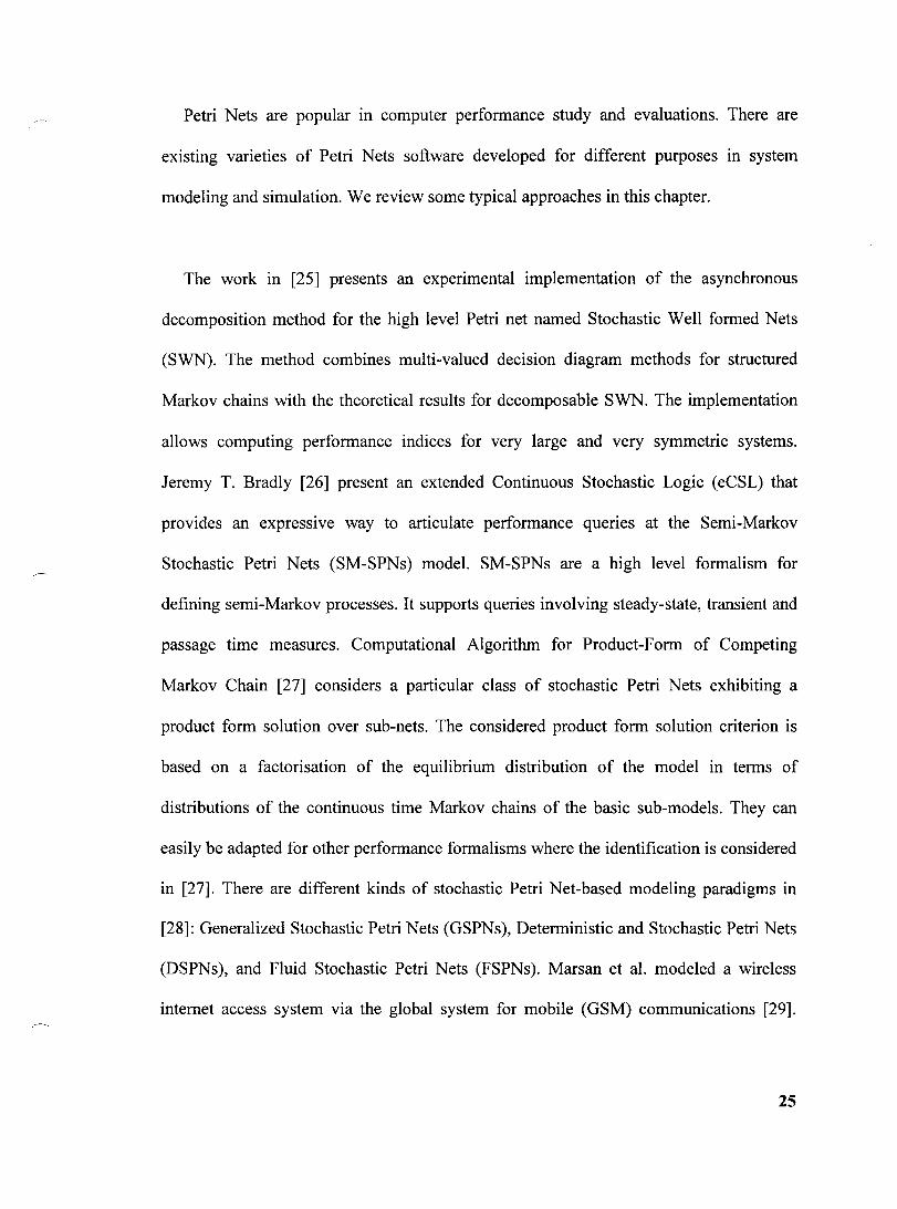
To solidify concepts, consider the subdivision of a tetrahedron. As shown in Fig. 3.1,

one method consists of cutting every edge into two and every face into four subtriangles

[38] [39]. This results in four tetrahedra, each a half-scale duplicate of the original, and

an octahedron, as shown in Fig.3.1. The resulting octahedron can, subsequently be

subdivided in various ways. For example, one approach is to cut it along its vertices from

one on top to another on the opposite bottom, so that each tetrahedron has one edge

which is the line joining these two vertices. However, these tetrahedra are no longer

similar to the original one. Another approach is to cut the Octahedron into 6 half-size

octahedra and 8 tetrahedra, as shown in Fig. 3.2 [38][39]. For this refinement scheme, the

34

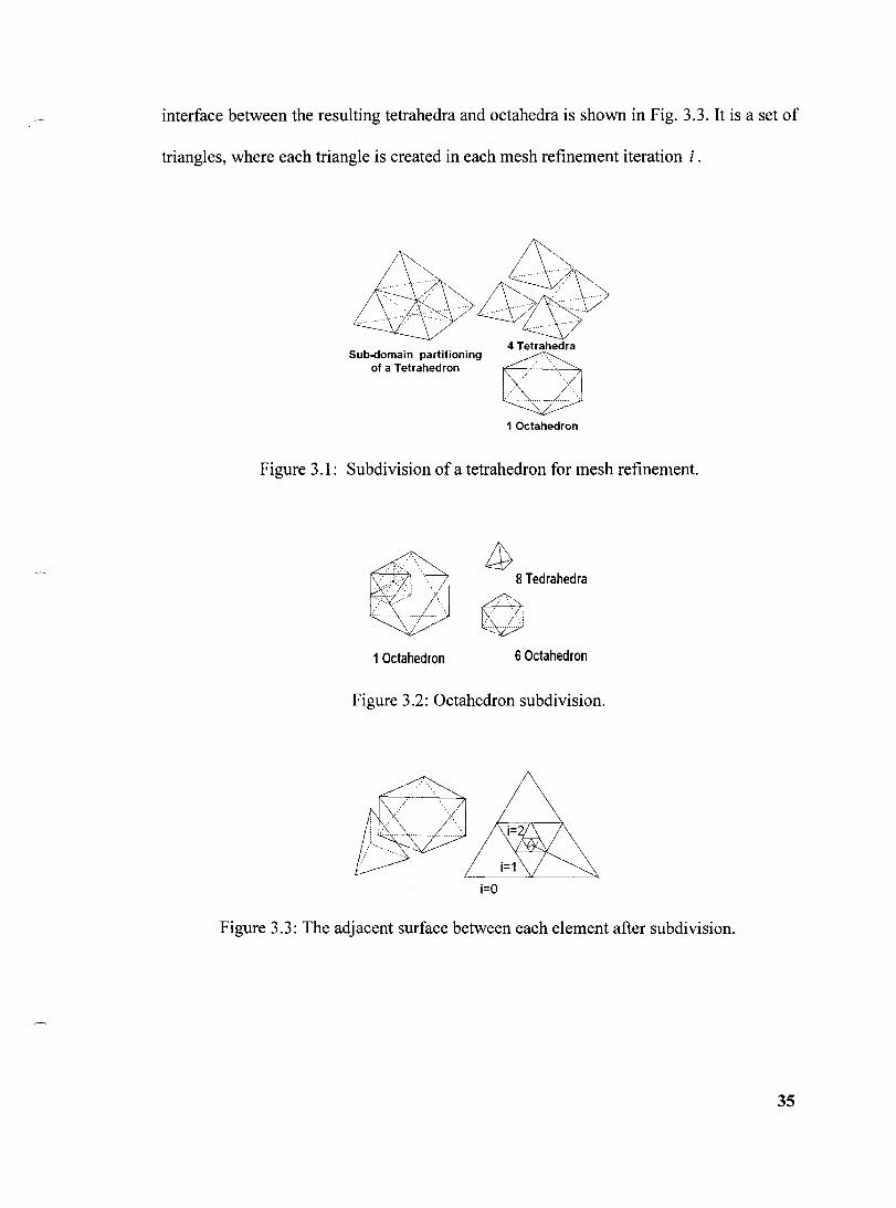
interface between the resulting tetrahedra and octahedra is shown in Fig. 3.3. It is a set of

triangles, where each triangle is created in each mesh refinement iteration i .

Figure 3.1: Subdivision of a tetrahedron for mesh refinement.

~:;'::;; ....

,,:,::<.::j :\ \, ~ ..... ----- ---------.. _-_ ...... :

W 8 Tedrahedra

~ 1 Octahedron 6 Octahedron

Figure 3.2: Octahedron subdivision.

i=O

Figure 3.3: The adjacent surface between each element after subdivision.

35

3.3 Parallel Algorithm Analysis

To parallelize the refinement strategy described in Section 3.2, each processor may be

assigned to one or more tetrahedra and octahedra. Computationally, the geometric model

can be described by a boundary representation consisting of free form entities: vertices,

curves, surfaces, and regions. We use the following terms in this paper:

i: Iteration number of each refinement;

7;: Number oftetrahedra at refinement iteration i;

0i: Number of octahedra at refinement iteration i;

Tpartitioning : Tetrahedron partitioning algorithm;

o partitioning : Octahedron partitioning algorithm;

The initial tetrahedron Ta in the ith (i ~ 1) refinement can generate 7; =47;-1 +8 0i-1 and

Oi = 7;-1 +6 OH . There are 5 computational steps in partitioning a tetrahedron and 14

steps in partitioning an octahedron. Thus the computation time and communication time

for a single processor p is

i-l

Pi (tcomputal;o n) = l (5Ti-! + 140;_1 +)t part (3.1)

(3.2)

36

Here {part represents time cost of one unit step of mesh partitioning. {startup is the startup

time, l.e. message latency. {data is the transmission time to send data of one element.

These parameters are dependent on the actual parallel computing system employed, and

can be assumed constant corresponding to the actual environment.

For p CPUs in a master-slave mode, there will be p -1 slave processors in charge of

p -1 sub-domains. The overall run time including communication will be

p

Toveral/ = max(p i (t computation)) + L Pi (t communication) i;1 (3.3)

The sub-domain partitioning is given in Table 3.1. Theoretical timing estimations are

given in Table 3.2 for the case {startup' {part and {data are constants.

Table 3.1: The sub-domain partitioning.

1 CPU 1 tetrahedron

3 CPUs Pl: 3 Tetrahedra; P2: 1 Tetrahedron+ 1 Octahedron

4CPUs Pl: 2 Tetrahedra; P2: 2 Tetrahedra; P3: IOctahedron

6 CPUs PI-P4: 1 Tetrahedron; P5: IOctahedron

37

Table 3.2: Theoretical timing estimations.

Overall Time (time units) Number of Elements

ICPU 3CPUs 4CPUs 6CPUs

5 15 Il 9 7

34 112 78 66 64

260 858 620 540 538 2056 6766 4968 4368 4366

16400 53910 39776 35064 35062 131104 430822 318288 280776 280774

3.4 Parallel Meshing Environments

A weU-known paradigm for paraUel computations is the divide-and-conquer approach.

It consists of solving a problem by dividing it into several sub-problems, solving the sub-

problems and then merging the partial solutions together [40]. In the case of our mesh

refinement model, the problem domain can be easily divided into a set of fairly balanced

sub-domains, i.e. the divide-and conquer approach divides each initial tetrahedron into

four tetrahedra and one octahedron, for a total of 5 entities.

The paraUelization strategy involves two levels: the model level (partitioning will be

done by the master processor of a multiprocessor system); and the entity level (single

processor assigned to a sub-domain). Specifically, the parallel mesh refinement

environment consists of: (1) a meshing algorithm run by a processing element assigned to

a sub-domain; (2) a data exchange and control substrate that implements low-Iatency

message passing among the processing elements (we model this based on the

communication functions in MPI); and (3) a global address space and automatic message

38

forwarding for load balancing (in a master-slave model, this will be handled by the

master processor). A conceptual diagram ofthis paraUel mesh refinement environrnent is

shown in Fig. 3.4.

The Master Proeessor

P-1 :number of slave proeessors beast(Graphic_Data. p-1. P _slaves); reev(): Wait for results from slaves;

Buildup new graphic file and rearrangement

The Slave Processor

1

beast(Graphic_Data. P-1. P _master); start meshing ........

Buildup new graphie file Send( Graphic_New. P _master)

1

The Slave Processor

bcast(Graphic_Data, P-1, P _master); start meshing

Buildup new graphic file Send( Graphic_New. P _master)

Figure 3.4: ParaUel mesh refinement environrnent.

The paraUel meshing scenario is straightforward. The initiaUy partitioned 4 tetrahedra

and one octahedron are first sent from the master processor to slave processors. The slave

processors load the Tpartitioning and 0 partitioning algorithms for subdividing the entity assigned

to them, operating independently and concurrently. Once an iteration is complete, the

output data is written back to the master processing element. The master processor will

merge the meshing surfaces between each sub-domain. FinaUy, the master processor adds

the partial meshes to form the result. The output of an iteration of mesh refinement will

be the input of the next iteration. For this work, the data dependency is managed by a

queue structure.

39

3.5 Modeling of Components

The Petri Nets simulation model is a specification of the parallei mesh refinement

system in terms of a set of states and events. Performing the simulation is, essentially,

mimicking the occurrence of events as they evolve in time and recognizing their effects

as represented by states during the parallel meshing. We selected two parts of our model

for illustrating our methodology. The entire model is available upon request. The first

part represents a processor assigned to a sub-domain, and is shown in Fig. 3.5. One

tetrahedron produces 5 entities. The nurnber of entities produced is defined in the model

by weights and the timing delay is defined in the transitions. The octahedron is among the

5 entities produced, and will be subdivided subsequently within the same iteration. The

number of elements is represented by tokens. Once the subdivision of the tetrahedron is

completed, a synchronizing token will be sent to the control part of the model. At this

time, the octahedron subdivision will commence. The control part will wait for the end of

the octahedron subdivision, and then one iteration is completed for the slave processor. A

token will be fired to the master processor and then aIl the data will be written back to the

master processor.

Fig. 3.6 shows the second part, which is the data collecting and broadcasting process

in the master processor for a 6 CPU system. The data writing delay is defined in the

transitions. Once aIl the data from slave processors have been collected at the end of an

iteration, the master processor will merge the results together. AIso, the data is distributed

to each slave processor for the next iteration of mesh refinement.

40

Tetrahedra Dis8ssemble

,'initiai TetrGl1eâa storage

1 , , , ,

1----------'1

- ......... '\

\ \ \ \ \ \ \ l , l i J

: o:tahedra Disassemble )4'+1 -+-_+--,

1

1"~iGl OctBh!~B

S'larage

Figure 3.5: Petri Nets model of a processor assigned to a sub-domain.

r 1

L

-----, Data Write Back ta 1 Master Processor _____ --.J

--------, Data Assembling :

1

1

1 _____ -.J

Broadcast Data to' Slave Processors 1 _____ --.J

Figure 3.6: Petri Nets model for master processor in 6 CPU system.

41

Table 3.3: Simulation results for 1,3,4 and 6 CPUs in a Mater-Slave model.

lCPU 3CPUs

Elements Number Simulation Time Elements Number Simulation Time

(time units) (time units)

1 36 16 36 14

2 624 198 624 162

3 10368 3174 10368 2598

4 171648 48046 171648 42918

5 2840832 867462 2840832 710214

4CPUs 6CPUs

Elements Number Simulation Time Elements Number Simulation Time

(time units) (time units)

1 176 30 176 18

2 2976 390 2968 198

3 49344 6342 48848 3174

4 816768 104838 171648 52422

5 13459588 1734918 13077128 867462

Table 3.4: Comparison ofload imbalance (number of elements).

1 CPU 3 CPUs 4CPUs 6CPUs

1 0 12 1 0

2 0 192 22 6

3 0 3168 372 20

4 0 52416 6168 1822

5 0 867456 102096 29120

42

3.6 Simulation Results

The performance results presented below have been obtained from the Petri Nets model

described above with the analysis tool Hpsim [41]. In the model, we set {part =2 and

{data =1 (time units). Table 3.3 presents the simulation results for parallel mesh refinement

using 1,3,4, and 6 CPUs ..

Fig. 3.7 shows a comparison ofmesh refinement estimation times (E-l, E-3, E-4, E-6)

with corresponding Petri Nets simulation times (R-l, R-3, R-4, R-6). We can observe that

the Petri Nets simulation results are in close agreement, to within a time constant related

the selection of system parameter values (part' (data and (startup in the Petri Nets model

that was used.

The time estimation curve of 6 CPUs, (E-6), is almost identical to the curve for 4 CPUs

(E-4). Similarly, there is sorne overlap of the 6 CPUs (R-6) and 4 CPUS (R-4) Petri Nets

simulation results. This may be attributed to the overall computation time being

determined by the most complex processor. In our case, they are P3 of the 4 CPUs system

and P5 in the 6 CPUs system (refer to Table 3.2).

The load balancing (see Table 3.4) in this case is closely related to the sub-domain

partitioning used. To minimize the algorithmic complexity, we partitioned the sub

domains by subdividing the original tetrahedron into 5 geometric entities, and assigning

one or more entities to each slave processor according to the total number of CPU s

43

employed. Obviously, computation In a 3 CPU system has the most senous load

balancing problem, because the sub-domains could not be created fairly. This is actually

a trade-offbetween load balancing and algorithmic complexity.

(IJ "-Q)

> 0

107r-----------.------------r-----------,----------~

102

101

_________________ ~ _________________ ~ _________________ 4 __ _

1 1 1 1 1 1 1 1

1 1 1

_ ........................... __ ............... L ...... __ ...................................... ! __ ...

-+- E-1-CPU + R-1-CPU ___ E-3-CPUs -B- R-3-CPUs ........ E-4-CPUs

.............................. ~ .................................................. !............................................ -A- R-4-CPUs 1 1

...... E-6-CPUs -e- R-6-CPUs

10° 10° 10

4

Number of Elements

Figure 3.7: Number of geometric entities vs. execution time.

3.7 Conclusion and Future Work

Parallel mesh refinement can be effectively described and analyzed using the timed

Petri Nets formalism. The system execution time and load balancing situation can be

estimated in our example. Future work should include utilizing Petri Nets for adynamie

44

load balancing protocol analysis, and more detailed communication cost analysis in order

to optimize parallel mesh refinement performance.

45

CHAPTER 4: Analysis and Design ofParallel3-D Mesh

Refinement Dynamic Load Balancing Aigorithms for Finite

Element Electromagnetics with Tetrahedra

Preface

The following chapter is inc1uded as a paper published by the IEEE Transactions on

Magnetics, Volume 42, Issue 4, Pages 1251-1254, April 2006.

The paper's role is to apply the Petri Nets methodology introduced in Chapter 3 for

modeling and simulating a Random Polling Dynamic Load Balancing (RPDLB)

algorithm for parallel Hierarchical Tetrahedral and Octahedral Sub-division mesh

refinement. The Performance of RPDLB is examined in this chapter, and through this

work the benefits of the PN approach for developing high performance parallel mesh

refinement algorithms are demonstrated and evaluated.

46

CHAPTER 4: Analysis and Design ofParallel3-D Mesh Refinement

Dynamic Load Balancing Aigorithms for Finite Element Electromagnetics

with Tetrahedra

Dennis D. Giannacopoulos and Da Qi Ren

Abstract:

We develop a simulation-based approach for the computational analysis and design of

dynamic load balancing algorithms in parallel, 3-D, unstructured mesh refinement with

tetrahedra. A Petri Nets model is implemented based on a random polling algorithm and

the target multiprocessor architecture, which simulates the behavior of the parallel mesh

refinement. Subsequently, estimates for performance measures are derived from discrete

event simulations. The benefits of this new approach for developing high performance

parallel mesh refinement algorithms are demonstrated with results for an example

geometric mesh refinement mode!.

Index Terms:

Adaptive systems, electromagnetic analysis, finite element methods, parallel

processing, software methodology.

47

4.1 Introduction


approximate solution of continuum electromagnetic problems. However, efficient and

accurate solutions for sorne 3-D modem applications require extremely large numbers of

elements. In such cases, parallel processing is beneficial for each stage of the FEM

including mesh refinement [40], [42], [43]. Due to the computational complexity of 3-D,

parallel, unstructured mesh generation and refinement, the performance of the method is

highly dependent on several factors, e.g., the underlying algorithm, the inter-processor

communication pattern, the synchronization of tasks, etc. The goal of modeling and

simulating parallel mesh refinement is to examine the specific parallel system

architecture and software techniques in advance, in order optimize its design and thus

achieve the best possible performance for a given cost.

Today, techniques used for parallel mesh refinement performance analysis are,

typically, based on benchmarking programs on known environments. Unfortunately,

these types of deterministic evaluations are inefficient for performance studies in the

early design stages of a parallel system. For example, various analysis and design

methodologies reported in the literature have been used to address separately specific

load balancing algorithms or mesh refinement models. In other words, these approaches

focus, typically, on only one particular aspect of a whole parallel mesh refinement system

[43]-[45]. Thus, such separately focused analyses, cannot predict the performance of the

whole parallel mesh refinement system accurately. One promising route for overcoming

48

these limitations is based on extending a preliminary approach developed previously by

the authors for using Petri Nets to simulate parallel mesh refinement [46]. In order to

obtain more accurate simulation results for the performance analysis of a whole parallel

mesh refinement system, the distributed data structure, geometric mesh refinement

model, dynamic load balancing (DLB) algorithm, parallel system architecture, and the

inter-processor communication details must all be incorporated in the Petri Nets model in

a realistic fashion. This type of holistic simulation is an original approach that we believe

willlead to improved analysis and design methods for parallel3-D mesh refinement DLB

algorithms for finite element electromagnetics.

In this paper, we develop a new approach for the modeling, analysis and design of

DLB algorithms in parallel finite element mesh refinement that utilizes Petri Nets. Petri

Nets-based models allow for a relatively detailed description of a system due to their

formaI syntax and functional semantics, and can reveal key characteristics of system

performance stochastically. While Petri Nets have been used for discrete event-based

simulation of various applications, to our knowledge, they have not been considered

previously for parallel 3-D mesh refinement DLB for finite element electromagnetics

with tetrahedra [46]-[48]. In addition, we use the proposed approach for the design of a

random polling (RP)-DLB algorithm for a specific 3D parallel mesh refinement model

suitable for FEM electromagnetics with tetrahedra [46], [48], [49].

49

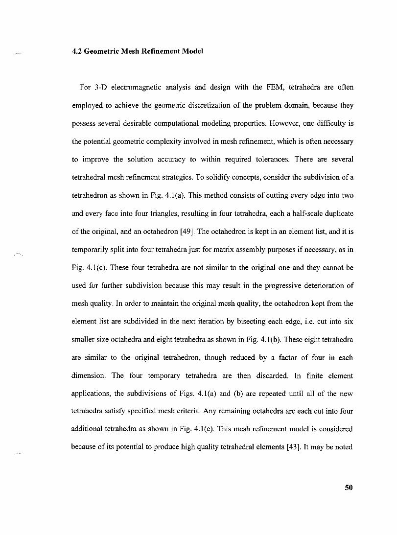
4.2 Geometrie Mesh Refinement Model

For 3-D electromagnetic analysis and design with the FEM, tetrahedra are often

employed to achieve the geometric discretization of the problem domain, because they

possess several desirable computational modeling properties. However, one difficulty is

the potential geometric complexity involved in mesh refinement, which is often necessary

to improve the solution accuracy to within required tolerances. There are several

tetrahedral mesh refinement strategies. To solidify concepts, consider the subdivision of a

tetrahedron as shown in Fig. 4.1(a). This method consists of cutting every edge into two

and every face into four triangles, resulting in four tetrahedra, each a half-scale duplicate

of the original, and an octahedron [49]. The octahedron is kept in an element list, and it is

temporarily split into four tetrahedra just for matrix assembly purposes if necessary, as in

Fig. 4.1(c). These four tetrahedra are not similar to the original one and they cannot be

used for further subdivision because this may result in the progressive deterioration of

mesh quality. In order to maintain the original mesh quality, the octahedron kept from the

element list are subdivided in the next iteration by bisecting each edge, i.e. cut into six

smaller size octahedra and eight tetrahedra as shown in Fig. 4.1 (b). These eight tetrahedra

are similar to the original tetrahedron, though reduced by a factor of four in each

dimension. The four temporary tetrahedra are then discarded. In finite element

applications, the subdivisions of Figs. 4.l(a) and (b) are repeated until all of the new

tetrahedra satisfy specified mesh criteria. Any remaining octahedra are each cut into four

additional tetrahedra as shown in Fig. 4.1(c). This mesh refinement model is considered

because ofits potential to produce high quality tetrahedral elements [43]. It may be noted

50

that the tetrahedral and octahedral refinement rules of Fig. 4.1(a) and (b) generate

tetrahedra of the same quality as the original [49]; however, this is not necessarily the

case when the sub-division rule of Fig. 4.1 (c) is applied to terminate the mesh refinement

process for FEM applications, and other mesh optimization techniques can be applied to

improve the quality of the resulting elements.

(a) 1 Tetrahedron 4 Tedrahedra 1 Octahedron

(b)~q©+j) 1 Octahedron 6 Octahedra 8 Tetrahedra 1 Octahedron 4 Tetrahedra

Figure 4.1: Mesh refinement model: (a) tetrahedron subdivision; (b) primary octahedron

subdivision; (c) secondary octahedron subdivision.

4.3 RP-DLB Parallel Mesh Refinement Model

In this section, the RP-DLB modeling strategy is briefly explained, and key algorithmic

details are given. A master-slaves parallel computing scheme is considered for this work.

A. RP-DLB Algorithm

1) Overview of Parallel Mesh Refinement with RP-DLB

Fig. 4.2 shows a conceptual outline of the key elements for our parallel mesh

refinement with RP-DLB algorithm. To begin, the input data are read, parsed, and

51

checked by the master processor. The initial geometric mesh model is then broadcast to

aIl slave processing elements (PEs), which, in tum, estimate their anticipated work load

and send it to the master PE. Model entities with an expected excessive work load are

split into smaller units by slave PEso During this phase, a RP-DLB mechanism is applied

[44]: while the work is not finished aIl slave PEs will work in parallei asynchronously;

however, if a PE's local tasks are done, it will repeat sending a request R to other

randomly determined PEs until R is not rejected. The "polled" PE will split its remaining

tasks and reinitialize them asynchronously as sorne are sent to the PE that initiated R .

Master PE

Broadcast complete domain decomposition and

sub-domain assignrnent to slave PEs

Slave PEs

Random Polling Dynamic Load Balancing among the slave PEs

Build up new data flle and send itback

to the master PE • • •

Build up new data flle and senditback

to the master PE

Figure 4.2: Conceptual outline ofparallei mesh refinement with RP-DLB.

o ::l (1)

A discrete events chart for the operation of a slave PE performing mesh refinement in

our model is shown in Fig 4.3; it is constituted of five states and eight transitions. The

slave PE starts with tasks assigned by the master PE, and subsequently its state will

52

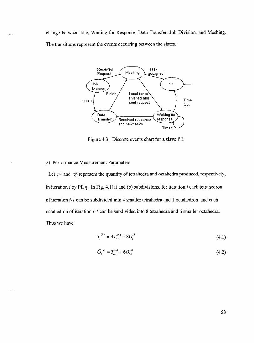
change between Idle, Waiting for Response, Data Transfer, Job Division, and Meshing.

The transitions represent the events occurring between the states.

sent request

Received response and new tasks

Time Out

Figure 4.3: Discrete events chart for a slave PE.

2) Performance Measurement Parameters

Let 7;(k) and qk)represent the quantity oftetrahedra and octahedra produced, respectively,

in iteration i by PE~. In Fig. 4.1 (a) and (b) subdivisions, for iteration i each tetrahedron

of iteration i-l can be subdivided into 4 smaller tetrahedra and 1 octahedron, and each

octahedron of iteration i-l can be subdivided into 8 tetrahedra and 6 smaller octahedra.

Thus we have

T(k) = 4T(k) + 80(k) i ;-1 ;-1 (4.1)

O(k) = r(k) + 6O<k) , 1-1 ,-1 (4.2)

53

In any iteration of the mesh refinement, if matrix assembly is required, aIl the octahedra

in the element list will be subdivided into 4 tetrahedra each as in Fig. 4.1 (c), and in this

case

T(k) = T(k) + 40(k) j ;-} 1-1 (4.3)

O(k) =0 1

(4.4)

Let tpart and Opart be the time required for a tetrahedron or octahedron subdivision, as

shown in Figs. 4.1(a) and (b), respectively. For iteration i, the computation time t;omp and

communication time çmm for p" are given by (4.5) and (4.6), respectively. Here tstartup

represents the message startup time and tdata is the transmission time to send the data for

one element. These parameters can be adjusted to simulate their effect on the parallei

computing environment performance. For n PEs in a master-slave model, there will be

n-l slave PEs in charge of n-l sub-domains. The time ti for the slave PEs to complete the

mesh refinement for iteration i satisfies (4.7), (since the PEs start the refinement iteration

i at the same time in our model) [51]. The proofis shown in Fig.4.4.

tomp

( ) = 5T(k)·t + 140(k) '0 1 Pk 1-1 parI 1-1 parI (4.5)

tomme )=t +(rk) +OCk))"t

1 Pk slartup 1 1 data (4.6)

n-I

ti ::; max(ttomp

(Pk)) + L (ttomm (Pk)) (4.7) k=1

A standard performance measure is the parallel efficiency E:

54

E = n.t W parallel(n,w)

(4.8)

where w is the size of the mesh refinement process measured in units of sequential

execution time, and tparalle/(n, w) is the parallel execution time for a system consisting of n

identical PEs [44]. In this work we examine the performance of our approach both with

respect to parallel speedup and efficiency.

B. Modeling Framework

Our Petri Nets model is a specification ofthe parallel mesh refinement system with RP-

DLB in terms of a set of states and events. Performance simulation involves modeling the

occurrence of events as they evolve in time and recognizing their effects as represented

by transitions of states during the parallel mesh refinement process[ 47], [48].

, :.

:Tcomm(P 1) : Teom", (Pli) :Teo .... (P 2)

PG~ ____________________ ~I ____ ~I ______ ~ __ -+-. , ,

Teo",p (P 1) :Teo .... (P 1) : P'-L __________________ L--JI ____ ~I ______ ~ __ ~ __

Tco",p (P 2) Teo",", (P 2):

" max(tcomp (Pk» L (t~omm(Pk»

k-1

Figure 4.4: Timing diagrarn for proof of (4.7).

-, , ,

55

Parallel Mesh Reflnem ent Discrete Events Simulation

The Geometty Entity Mesh r----- Support Functions Refme ment Algorithm Layer 3

'" +

Parallel Computing Sehe me Diserete Events Modeling Load Balane ing Algorithm f+----. SynchrolÙZation Simulation Layer 2

"- + Me$age Passing Intenace

~ Model of Timed TIallSitions

Parallel System Structure Parameters S etup Layer 1

Figure 4.5: Framework for mesh refinement Petri Nets model.

We map the algorithm with the supporting formulae (4.1)-(4.7) into the Petri Nets

model by modifying the parameters related to the states, events and transition delays. The

parallel mesh refinement process can be conceived at three levels, each corresponding to

one layer of our Petri Nets model, as shown in Fig 4.5. The first layer comprises the

parallel computing environment module. The parameters involved in this layer are the

communication timing delay and computation cost. The value estimation of the

parameters are conc1uded from the system implementation (we use the MPI of SUN

HPC5.0). The corresponding part in the Petri Nets model is the timed transitions. Layer 2

is the parallelization and load balancing algorithm module. The specification of the

processor interactions and the DLB schemes is built up in this layer. In the Petri Nets

model, this part is the discrete events logic. Layer 3 is the application layer. The

geometrical properties of the tetrahedral and octahedral subdivisions are specified in this

module. On the right, for the same layer of the Petri Nets model, we use the transition-

arc-weight to model the geometrical mesh refinement scheme. The details of the model

are provided below.

56

C. Petri Nets Model

1) RP-DLB Protocol

FigA.6 (a) shows the Petri-Nets model of the RP-DLB proto col. In a PE, tasks to be

executed are stored in Data _ Storage, while the geometric computations are being

processed. When a request R arrives, the PE wiU send half of the tasks in Data _ Storage to

the sender of R. When the PE has executed aU the tasks in Data Storage, it will send R to

another randomly selected PE and simultaneously start to build up a new data file.

2) Meshing Computation

The Petri Nets model in Fig.4.6 (b) shows the procedure of tetrahedral and octahedral

subdivision: this starts with a scan of tetrahedral/octahedral entities; next the refinement

rule is applied to each individual tetrahedron/octahedron. Once an individual element is

processed, a signal is generated by Scan Trigger for loading the next geometrical entity.

3) ParaUel System Model

The overaU model we developed is shown schematicaUy in FigA.7. It involves six

modules, representing one master and five slave PEs that we have in a symmetric

multiprocessor. The communication costs are defined by transitions that connect the PEs

in the system, as shown in the figure. The system parameters (part, 0part, (data, and (startup,

are defined in the transition delays in each stage of the mesh refinement model.

57

Request Received ~-------~-------~ • )----t---fI._ If the task pool Il Building up the new data file 1

is not empty 1 1 spltt half of 1 T35

l4----i __ the tasks. Il

fseparated Tasks

1 o 1 Half of the task

splitto the 1 request sender 1

1

another half remain local hosto

1

l ____ ~_~=-1 -+-__ ...... --~ Send Request

(a)

(b)

P26 1

-------1,-;--------, Il T elrahedra 1 1 1 1

Data Wr~e 1 Il 1 Octahedra 1 1 Baek 1 Data Write 1

1 Back 1

1 1

1 1

1 J

-----, 1

Geomelry Sean Trigger: T elrahedra 1

1 1 Part~io~ing Done

Figure 4.6: Petri Nets Module: (a) RP-DLB task sub-division; (b) tetrahedron and

octahedron sub-division.

58

3) Parallel System Model

The overall model we developed is shown schematically in Fig.4.7. It involves six

modules, representing one master and five slave PEs that we have in a symmetric


in the system, as shown in the figure. The system parameters tparr, Opart, tdata, and tstartup,

are defined in the transition delays in each stage of the mesh refinement model.

4.4 Results

The efficiency of a RP-DLB algorithm specifically designed for the mesh refinement

model described in this work is examined in this section. Performance results for the RP

DLB parallel mesh refinement simulation are shown in Fig.4.8. It may be noted from Fig.

4.8(a) that the parallel speedup for different numbers of PEs differs with increasing

problem size as the mesh refinement progresses. In each case, RP-DLB improves the

performance compared to the same number of PEs without DLB. Furthermore, it can

bene fit the system by saving PEs: (e.g., 5 PEs with RP is as good, or better, than 6 PEs

without RP). Fig. 4.8(b) shows the parallel efficiency versus the number of PEs in the

system. The results are based on the mean speedups observed over the entire range of the

number of elements produced during the refinement procedure. Clearly, the parallel

efficiency of the new RP-DLB mesh refinement model is better than without load

balancing. In addition, note that the parallel efficiency increases as the number of PEs

increases up to the 6 PEs in our model.

59

r------l 1 1

1 ~::= 1 1 1 1 1 1 1 1

1

1

1

1

1

1

1

1

1

1

1

1

1

1

1

1

1

1

1

1

1

1

1

1

1

1

1

1

1

1

1

1

1

1

1

1

1

1

1

1

1

1

1

1

1

1

1

1

1

1

1

1

1

1

1

1

: (a) : L ______ -.J

Figure 4.7: The Overall structure ofPN model for parallel mesh refinement in a 6 PE

system. (a)Workload Reassigning; (b) Polling Process. (Note: this is a complete version

of the original figure in the paper.)

60

~

5.5

5

4.5 6 PEs

4

3.5 a. ::J 3 "'0 <D ~2.5

CI) 2

1.5

3 PEs

0.5

° (a) 102

103

104

105

Number of Elements 10

6

0.9 ............... -- -- ---- ------:-- ---- ----~------- --~- ---- ---- -:--- ... _-- ---~--_ ... --- ...

0.8 ---------

>uO.7 c: <D

ë:; 0.6 ~ W _0.5 <D

~0.4 (0

a.. 0.3

0.2 ---------

0.1 ---------

, , , , : No Load ~alancing qontrol

---- ...... -- --,-- ......... --- -r-- ---- ... -'''' ---- ... ----,--- ---- ---r ---- ----, , , , , , 1 1 1 1

1 1 1 1 1

... -_ ... ---_ ... -:- ----- --~ ... -- --_ ... --~----- ---- -:--- --- --_ ... ~_ ... ---_ ...... 1 1 1 1 1

1 1 1 1

-------- -~-- ------~---------~---------~----------~--------1 1 1 1 1 , , , , , , , , ,

107

O~----e_----~----~----~------~----~----~

(b) ° 3 4 Number of PEs

7

Figure 4.8: RP-DLB performance results: (a) speedup vs. number of elements for

different numbers of PEs; (b) parallel efficiency vs. number of PEso

61

4.5 Conclusion

A new approach for the modeling, analysis and design of DLB algorithms in parallel

finite element mesh refinement that utilizes Petri Nets has been proposed and evaluated.

This new simulation-based approach allows for a relatively detailed description of a

system and can reveal key performance characteristics. The results for the 3D parallel

mesh refinement model considered demonstrate the benefits of the new approach for

developing RP-DLB algorithms for the target parallel architecture. Future work should

include further performance optimization of the new RP-DLB parallel tetrahedral mesh

refinement algorithm for systems of heterogeneous multiprocessors and through a more

detailed communication cost analysis. Finally, the new modeling approach may be

extended to other aspects of the FEM, such as matrix assembly and solution methods.

62

CHAPTER 5: Parallel Mesh Refinement for 3-D Finite

Element Electromagnetics with Tetrahedra: Strategies for

Optimizing System Communication

Preface

The following chapter is included as a paper published by the IEEE Transactions on

Magnetics, Volume 42, Issue 4, Pages 1235-1238, April 2006.

Continuing with the aim of improving the parallel mesh generator's performance, the

workload prediction approach, which is a new pipelined communication design, is

introduced in this chapter. The Petri Nets methodology form Chapter 3 is applied to

model and simulate this new workload prediction pipelined communication approach

through a case study in parallel Hierarchical Tetrahedral and Octahedral Sub-division

mesh refinement. The performance efficiency of the new design is examined.

63

_/--

CHAPTER 5: Parallel Mesh Refinement for 3-D Finite Element

Electromagnetics with Tetrahedra: Strategies for Optimizing System

Communication

Da Qi Ren and Dennis D. Giannacopoulos

Abstract:

Communication strategies in parallel finite element methods can greatly affect system

performance. The communication cost for a proposed parallel 3-D mesh refinement

method with tetrahedra is analyzed. A Petri Nets-based model is developed for a target

mesh refinement algorithm and parallel computing system architecture, which simulates

the inter-processor communication. Subsequently, estimates for performance measures

are derived from discrete event simulations. The potential benefits of this approach for

developing high performance parallel mesh refinement algorithms are demonstrated by

optimizing the system communication costs for varying problem size and numbers of

processors.

Index Terms:

Adaptive systems, electromagnetic analysis, finite element methods, parallel

processing, software methodology.

64

5.1 Introduction

The accuracy and efficiency of approximate solutions obtained with the finite e1ement

method (FEM) for practical electromagnetic problems can be highly dependent on 3-D

mesh refinement algorithms. Advances in parallel computing have made higher fidelity at

finer solution resolution possible. However, inter-processor communication costs in

parallel FEM can greatly degrade the system performance and diminish the potential

benefits of utilizing increased numbers of processors. The communication cost in paralle1

mesh refinement is dependent on the underlying computational algorithm as well as the

system architecture. The objective of analyzing paralle1 communication paradigms for

specific architectures in advance is to optimize use of system resources and improve

performance.

In this paper, we develop a new approach for the modeling, analysis, and design of

communication schemes in parallel finite e1ement mesh refinement that utilizes Petri

Nets. Petri Nets-based models allow for a relative1y detailed description of a system due

to their formaI syntax and functional semantics, and can reveal key characteristics of

system performance stochastically. While Petri Nets have been used for discrete event

based simulation of various applications, to our knowledge, they have not been

considered previously for communication costs in paralle1 3-D FEM mesh refinement

[46]-[48]. In addition, we use the proposed approach for the optimization of the

communication strategy for a 3-D paralle1 mesh refinement model suitable for FEM

e1ectromagnetics with tetrahedra [49], [51].

65

5.2 Parallel Mesh Refinement Approach

Tetrahedra are employed frequently in 3-D electromagnetic analysis and design with

the FEM to achieve the geometric discretization of the problem domain. Several

tetrahedral mesh refinement schemes are possible to improve the solution accuracy

required for engineering tolerances [51]. To solidify concepts, consider the subdivision of

a tetrahedron indicated by Fig. 5.1. This refinement rule initially subdivides a tetrahedron

into four scaled duplicate tetrahedra and one octahedron as shown in Fig. 5.1(a). Next,

the octahedron is further subdivided into six octahedra and eight tetrahedra, as illustrated

in Fig. 5.1 (b). Finally each octahedron from Fig. 5.1 (b) will be subdivided into four

tetrahedra as shown in Fig. 5.l(c) [40], [43], [46], and [49].

A master-slaves parallel computing model is assumed for implementing the mesh

refinement method considered in this work [40], [46]. The master processing element

(PE) initiates the pro gram by checking the input data, gathering load information from

slave PEs, and partitioning the initial set of geometric entities into sub-domains. The

master PE then broadcasts the complete domain decomposition data and sub-domain

assignments to corresponding slave PEs, which proceed with the mesh refinement of their

assigned sub-domains, as shown in Fig. 5.2. The time for each slave PE to finish

receiving a workload assignment from the master PE may not be the same because of

differences in the workloads and communication delays. At this stage, the master PE will

wait until each slave PE has acknowledged complete receipt of its workload assignment.

Next the master PE broadcasts an instruction to aIl slave PEs to (approximately)

66

synchronously start parallel computing [51]. The slave PEs executing the tetrahedral-

octahedral subdivision algorithm (Fig. 5.1) work in parallel independently in each

domain. When a slave PE completes its local tasks its data are written back to the master

PE, where data from each sub-domain is merged to form the global result for the overall

problem domain.

~ ~~ (a) ~qLl>~+ ~

1 Tetrahedron 4 Tedrahedra 1 Octahedron

(.)~q©+4 1 Octahedron 6 Octahedra 8 Tetrahedra 1 Octahedron 4 Tetrahedra



MasterPE Slave PEs

1 Reac!, parse and check input data l ~ .... 0+ .... Ilol .... ....

1 Broadcast model description to slave PEs Rece ive model description l N Ilol

l l 0+

o' 1 Loon Start l ~

l l - ---_ ..

( Broadcast complete domain decomposition Receive complete domain decomposition ......

0+

and sub-domain assignment to slave PEs Receive sub-domain assignrnent Cl)

'"' l ~.

1 0

Refme mesh on assigned sub-domain ~ II>

and build up new data flle 0 ..., l El

1 Rece ive new data file fro m all slave PEs Send new data file back to the master PE l Cl) II>

1 ::r '"'

1 Checking data and scheduling new iteration J Cl)

~ 1 Cl)

1 Loon End l El l Cl)

1 Write output data ofmeshes J a

Figure 5.2: Parallel mesh refinement approach.

67

5.3 Communication Model

In this section, a Petri Nets-based communication model is developed for the parallel

mesh refinement strategy considered. Let T,(k) and d;k) represent the quantity of tetrahedra

and octahedra produced, respectively, in iteration i by PE ~ . In Fig. 5.1(a) and (b)

subdivisions, for iteration i each tetrahedron of iteration i-1 can be subdivided into four

smaller tetrahedra and one octahedron, and each octahedron of iteration i -1 can be

subdivided into eight tetrahedra and six smaller octahedra. Thus we have

r(k) = 4r(k) + 80(k) i ;-} ;-1 (5.1)

O(k) = r(k) + 60(k) 1 1-1 1-1 (5.2)

In any iteration of the mesh refinement, if matrix assembly is required, each octahedron

in the element list will be subdivided into four tetrahedra as in Fig. 5.1 (c), and in this case

r(k) = r(k) + 40(k) 1 I-} 1-1 (5.3)

O(k) = 0 1 (5.4)

Let tpart and Opart be the time required for a tetrahedron or octahedron subdivision, as

shown in Figs. 5.1(a) and (b), respectively. For iteration i, the computation time tjcomp and

communication time çmm for ~ are given by (5) and (6), respectively [51].

68

tomp ( ) = 5T(k) . t + 140(k) . 0 1 Pk 1-1 part 1-1 part (5.5)

t comm ( ) = t + (T(k) + O(k)) . t 1 Pk starlup 1 1 data (5.6)

Here t"ar'ur represents the message startup time and t dala is the transmission time to send the

data for one element.

For n PEs in a master-slave model, there will be n-l slave PEs in charge of n-l sub-

domains. Let t,-'(po)be the time for the master PE po to broadcast sub-domain workload

assignments to an slave PEso In total, n processors participate in the broadcast operation

and the broadcast procedure involves log(n) point-to-point simple message transfers [51],

each at a time cost of t'tartup +tdata '(0;-1 + 1";-1)' Therefore, the total time taken by the

procedure is

(5.7)

The time I, to complete the mesh refinement for iteration i satisfies (5.8)-(5.9). The proof

is given in the timing chart of Fig. 5.3.

.-1

t < t comm () (t comp ( )) " (t comm ( )) i - i Po + max i Pk + ~ i Pk (5.8)

k=1

t> (tcomm

() t comp( )) i - max i Pk + i Pk (5.9)

69

After each iteration of its computationalloop (Fig. 5.2), a slave PE performs point-to-

point communication to send data back to the master PE. As shown in the timing chart of

Fig. 5.3, a PE's communication will be potentially blocked until another PE has fini shed

sending/receiving data to/from it (point A and B). It would be preferable if we could

overlap the transmission of these blocks with the computation for the mesh refinement, as

many recent distributed-memory parallel computers have dedicated communication

controllers that can perform the transmission of messages without interrupting the PE's

cpu.

, ,

Po 1 , c===]

, , 1 1

1 j t,.comp(p\) P1 t==d P2

1 1 t j

comp(P2)

~l Pk , t/omp(p,.)

1 1

tcomm~o).--- max(tcomp(Pk» , . '

B: .. 1 1 1 •

n 1

--._,'-2: (t/om"'(Pk» i , k=!

Figure 5.3: Timing for parallel mesh refinement in typical master-slave model.

5.4 Pipelined Communication Design

A pipelined communication strategy is designed for our mesh refinement scheme,

which overlaps communication and computation in order to avoid inter-processor

communication blocks (as described above). Briefly, the idea is to adjust the workload

assigned to each PE so as to create load imbalances in the of sub-domain partitioning

stage. The load imbalances will result in differences in computation times for each PE.

This time difference between PEs is used for overlapping (pipelining) one PE's

70

computation time with the data transmission time of another PE. This is illustrated in

Fig. 5.4.

respectively. The difference in computation time between Pk and Pj is tjcomf..p)_tjcom'(A)

(assuming that Pk finishes its computation first). Thus, the overlap in the communication

time for Pk' in this case, is given by (5.10). When Pk finishes its computation it starts

transferring result to the master PE Pa, while Pj keeps computing results for its domain.

After tjcom~)_({)mf..pk)' Pk completes its data transfer and Pj finishes computing, and then

Pj starts sending data to Po . The time slot tjcomf..p)_tjcomf..pk) allows pipelining the

communication of Pk and computation of Pj. To achieve this communication pipeline

that satisfies (5.10), the appropriate difference in workloads between Pk and 1'; must be

determined, and is given by (5.11); where IJ.1';_1 and IJ.0i _1 are the required differences

in quantities of the input tetrahedra and octahedra, respectively, between the two PEs

~and~.

( (k) 140 (k») t startup + 51(i-l) + (i-I) • t data

= 5 . t part· (1';-1 (j) - 1';-1 (k») + 14 . 0 part· (0(i-I) (j) - 0(i-I) (k»)

= 5 . t part • IJ.1';_1 + 14 . 0 part • IJ.0i _1

(5.10)

(5.11)

71

Po 1 1 j

P1 t==J!

i i t/ommcbl)

1 l , 1 1

P2 1 • 1 Il

: :t.·om",~:) 1 .2 ~

1 1 Pk 1

1 1 1

n 1 -+- L (t/omm(pk»-' . k-l •

tjcomm(po):_ max(tjCOmp(Pk»

Figure 5.4: Timing for pipelined communication design.

It should be noted that, the sub-domain workload adjustment is justified based on the

properties of the refinement rule in Fig. 5. 1 (a)-(c). That is, each element is covered

exactly by its parent element, and all meshes in the hierarchy are conforming (no hanging

nodes exist). Thus, the rule can be applied to neighbouring elements in adjacent sub-

domains without mesh consistency problems [43], [46], [49], [52].

5.5 Petri Nets Model and Simulation

The Petri Nets simulation developed for our parallel mesh refinement algorithm

involves modeling the occurrence of events as they evolve in time and their effects as

represented by transitions of states during the parallel mesh refinement process. We map

the algorithm with the supporting formulae (5.1)-(5.11) into the Petri Nets model, which

involves six modules: one master and five slave PEso The Petri Nets Model and initial

sub-domain distribution table are shown in Fig. 5.5 and Table 5.1, respectively. A

representative workload adjustment between two slave PEs is shown in Table 3.2, and the

corresponding Petri Nets module is shown in Fig. 5.6. The communication costs are

defined by transitions that connect PEs in the system together (Fig. 5.5). The system

72

parameters {part, Opart, {startup and {data are defined in the transition delays in each stage of

the computation and communication model. Note that the computation time of the mesh

refinement processes is comprised of tetrahedron and octahedron subdivision and data

preparation. An individual module named 'Co-Module' was developed for modeling this

computation time. In both Fig. 5.5 and Fig. 5.6 the 'Co- Module' is abbreviated as a

transition, namely "computation time".

Table 5.1: Workload Assignment:

T and 0 represent the number oftetrahedra and octahedra, respectively, assigned to each

slave PE at the 2nd or 3rd iteration refinement.

3 PEs 4 PEs 5 PEs 6 PEs

2nd iteration 3rd iteration 2nd iteration

PO: Master PO:Master PO:Master PO:Master

Pl:T=3 Pl:T=2: Pl:T=8,0=2 Pl:T=l

P2:T=1,0=11 P2:T=2 P2:T=8,0=2 P2:T=1

P3:0=1 P3:T=4,0=3 P3:T=1

P4:T=4, 0=3 P4:T=1

P5:0=1

73

r PE1

1

1

1

1

1

1

1

1

1 lime to Return New Data File L ________ _

T_data=l T-part=5 O-part=5

T_startup=100

Figure 5.5: Petri-Nets parallel communication model for 6 PEso

Table 5.2: Number of Elements:

M(i) is the total number oftetrahedra and octahedra to be adjusted between two slave

PEs at iteration i+ 1. F(i) is the final number oftetrahedra for iteration i after performing

the refinement mIe in Fig. 5.l(c).

Iteration MU) T(i) OU) FU)

4 52 176 84 512

5 410 1376 680 4096

6 3277 10944 5456 32768

7 26215 87424 43680 262144

8 209716 699136 349504 2097152

1 1

1

1

1

1

1

J

74

T_startup=100 Assignment 8roadcasting

T_data=l T ---.P art=5 o ---.P art=5

~---------------~~I---~.

start Receiving T asks P48

• )----...... _1--.,..; r.----i_ .... --------{ • o

Data Transfer

Time to Return New Data File Time to Return New Data File

Figure 5.6: Petri Nets module for pipelined communication of Pk and Pj .

5.6 Results

The performance results of the Petri-Nets simulations for 3 to 6 PEs are shown in

Fig. 5.7 (non-pipelined) and Fig. 5.8 (pipelined). It may be noted from Fig. 5.7(a), that

when the message size is greater than a specifie value (~ 450,000 bytes) the system

communication costs for 5 or 6 PEs are less than for 3 or 4 PEso This is due to the

'natural' pipelining effect caused by the increased number ofPEs, so that communication

and computation overlap to decrease the number of block points. Fig. 5.7(b) shows the

load imbalance ratio for different numbers of PEs over the range of communication costs

considered. The load imbalance ratio is the difference in work load between PEs divided

by the total work load in a given iteration i. Load imbalances cause PEs to complete their

individual tasks asynchronously, and can slow down the parallel computing speed.

75

However, differences in computing ending times can allow for effective overlap of

computation with communication, which can reduce the overall communication cost. It

may be noted from Fig. 5.7(b), that for a given system communication cost, different load

imbalance ratios result for different numbers of PEso This information is useful for

optimizing the design of the communication component of our mesh refinement strategy.

The corresponding results for the new pipelined design are shown in Fig. 5.8. The

curves in Fig. 5.8 (a) are ordered consistently, because the designed pipelined

communication is scheduled intentionally to optimize system resources. For example, the

communication cost for 6 PEs is greater than those for 5, 4, or 3 PEs at each iteration,

because the parallel scheduling is controlled and increases in complexity with the number

ofPEs. The system communication costs are comparable with Fig. 5.7(a) until the fourth

iteration, because the parallel scheduling cost is relatively large for smaller message

sizes. However, there is a significant reduction in cost for the new pipelined design

beginning with the fourth iteration. Fig. 5.8(b) shows a consistent increase in the load

imbalance ratio for increasing PEs, as the system overlaps more computation and

communication time. This is in agreement with the observation above: having more PEs

incurs more scheduling cost. However, this is a beneficial trade off required to avoid the

block points in the system.

76

---. (J)

"'C C o u Q) (J) o U ~ iiî o u c o .~

.S? C :::J

E E o u ~

106

105

~ 3 PEs ~ 4 PEs -.....- 5 PEs 1 1 1 1 -- 6 PEs -a-

------r-----------T-----------T-----------y----------. Q PEs

. . . -----------r-----------r-----------y----------. .

o (J) (J) Q)

u

e 101 D..

:5i ë

100~~~~~~~~~--~~~~~~~~~~~~~~~~ 101 102 103 104 105 106 107

Message Size (bytes)

106r-------O'========1------~--------r_----~

: -.....-------------,

3 PEs 4 PEs 5 PEs 6 PEs • -a-

5 PEs · -------------~--------------~-------------~ · .

· · . -------------,--------------~-------------

. - -----------~--------------~----------· .

100~~-------L--------~----------L---------~--------~ o 0.005 0.01 0.015 0.02 0.025

Load Imbalance Ratio

Figure 5.7: Performance results (without designed pipeline): (a) communication cost;

(b) load imbalance.

77

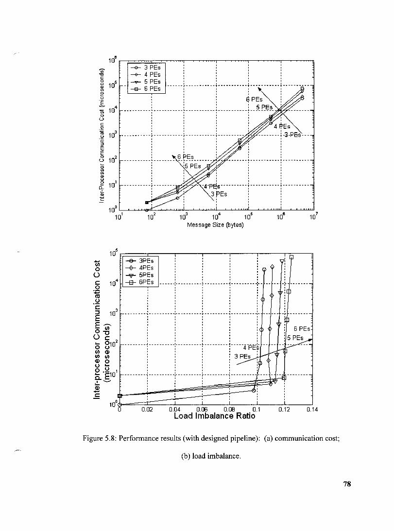
,,-... (1)

"'0 c: o u Q) (1)

~ u g (ï; o

Ü c: .'2 co u 'ë ~

E E o

ü

o

106~~~~==~~~~~~~~~:-~~~:-~~~ -&- 3 PEs ----+- 4 PEs , -;0- 5 PEs , ,

1 1 1 1

-a- 6 PEs ------r-----------T-----------T-----------T----------

Q PEs , , , , : : : : 5 PEs 1 ___________ L ___________ L ___________ ~ ___________ ~ ______ ___ _

,

, , , -----------r-----------r-----------T----------

, , , -------~-----------~----------, ,

(1) (1) Q) u

~ 101 0.... o!. Q)

ë

-(1)

o Ü

Message Size (bytes)

, , ,

~ 3PEs --+ 4PEs ~ 5PEs -;3-- 6PEs ........ .. -: .................... ~ .............. ... -,- .................. -:- - -:- --- ... ----: , , , ,

, : (

---------,----------~---------r---------,---------~-, , , , , ,

ui[

--------, u ~ J

: ( 6 PEs

----- --- -~ -------- --1- ---- ---- -~ -------- -1- ----4 -pË-1------:~ 3 PEs : .......-~!;1

, j t-'t:~" { : : : : ~ :~~

---------1- --------+ --------- r ----- ----1- --------1---- - -:i~- --- --- -"'"

~:

10011~::::::::~;;j,~====t,,=====Ji======li: ____ ~lL_ __ ~ o 0.02 0.04 0.06 0.08 0.1 0.12 0.14

Load Imbalance Ratio

Figure 5.8: Performance results (with designed pipeline): (a) communication cost;

(b) load imbalance.

78

5.7 Conclusion

A new approach has been proposed and evaluated that utilizes Petri Nets as a modeling

formalism for the analysis and design of communications strategies for parallei finite

element mesh refinement systems. Modules have been developed for modeling each stage

of the parallei algorithm, as weIl as the structure of the parallei system. The benefits of

the new approach for overall system performance evaluation and design optimization are

illustrated by the results for the new pipelined communication algorithm considered.

Future work should include further performance optimization of the computation and

communication cost in parallei FEM mesh refinement algorithm as weIl as other aspects

of the FEM.

79

CHAPTER 6: Efficient Pipelined Communication Design

for Parallel Mesh Refinement in 3-D Finite Element

Electromagnetics with Tetrahedra

Preface

The following chapter has been submitted to the IEEE Transactions on Magnetics.

Another new pipelined communication approach called the Task Break Point

approach, which is fundamentally different from the workload predication approach in

chapter 5 is introduced in this chapter. Once again the Petri Nets methodology of chapter

3 is applied to model and simulate this new approach in the case of parallel Hierarchical

Tetrahedral and Octahedral Sub-division mesh refinement. The performance efficiency of

the Task Break Point approach is examined.

The benefits of the PN approach for developing high performance parallel mesh

refinement algorithms are also demonstrated and evaluated in regards to chapter 1-3.

80

CHAPTER 6: Efficient Pipelined Communication Design for ParaUel Mesh

Refinement in 3-D Finite Element Electromagnetics with Tetrahedra

Da Qi Ren, Dennis Giannacopoulos and Steve McFee

Abstract:

Minimizing communication latency is an essential aspect of designing co st-effective

parallel finite element methods (FEM). A new, efficient pipelined communication

strategy that significantly reduces latency for parallel 3-D finite element mesh refinement

with tetrahedra is proposed. A Petri Nets (PN) based model is developed to simulate the

inter-processor communication costs for both the target mesh refinement algorithm and

parallel architecture. Performance measures derived from discrete event simulations

show that the new pipelined design yields improved communication speedup for a range

of refinement problem sizes, using different numbers of processors. In addition, the

potential benefits of using the PN-based model simulations for optimizing utilization of

the parallel system resources are demonstrated.

Index:

Parallel processing, finite element methods, mesh generation, Petri nets.

81

6.1 Introduction

ParaUel tetrahedral mesh refinement can be use fui for the modeling and simulation of

complex electromagnetics problems that require very large numbers of elements to obtain

high-accuracy 3-D finite element results. However, with sorne formulations, significant

inter-processor communication costs can significantly degrade system performance and

diminish the potential benefits of the paraUel processing approach. Further,

communication costs in paraUel mesh refinement are strongly dependent on the

underlying computational algorithm, as weU as the computational system architecture.

Therefore, accurately modeling and simulating the performance of communication

schemes in advance can help to yield improved paraUel speed-up, by optimizing the use

of the available system resources [53]. Recently it was shown that PN-based modeling

approaches can aUow for specific and detailed representations of paraUel mesh

refinement algorithms, which can be used effectively to reveal key characteristics of

paraUel system performance [46], [47], [53], and [54].

The primary objective of this contribution is to introduce a new and efficient pipelined

paraUel processing communication strategy for tetrahedral FEM mesh refinement. The

method is designed to minimize inter-processor communications latency, in order to limit

the potential performance degradation that can occur in paraUel tetrahedral mesh

refinement implementations. The new pipelined strategy is fundamentaUy different from

the communications strategies the authors reported earlier, and in particular, the previous

82

ca1culation and assignment of specific net workload imbalances for the processors is not

required [53].

A PN-based model is developed and used to investigate the performance of the new

pipelined communications design with detailed simulations of practical mesh refinement

applications, for a range of mesh sizes, and different numbers of processors. The parallel

processing performance characteristics of the new design are evaluated and compared to

non-pipelined methods, to assess the reduction in communications latency that can be

achieved and the potential impact on overall parallel speedup.

6.2 Parallel Hierarchical Tetrahedra and Octahedra Subdivision

Tetrahedral elements are often used in 3-D electromagnetic FEM to represent the

geometric discretization of the problem. Several tetrahedron refinement schemes are

possible for FEM applications, ranging from basic bisections to nested multi-cut

refinement schemes designed to preserve different aspects of the geometric quality of the

resulting mesh. To fix concepts, consider the subdivision of a tetrahedron illustrated by

Fig. 6.1. This refinement rule involves three steps: first, the tetrahedron is broken down

into four scaled duplicate tetrahedra (one for each corner) and one octahedron

(remainder) as shown in Fig. 6.1(a). Second, the resultant octahedron is then subdivided

into six octahedra and eight tetrahedra, as illustrated by Fig. 6.1 (b). Finally each of the

octahedra from Fig. 6.1 (b) is subdivided into four tetrahedra as given in Fig. 6.1 (c) [46],

[49], [53], and [54]. The recursive application of these tetrahedral and octahedral

83

refinement rules generate elements that belong to two congruence classes: one consisting

of all generated tetrahedra, and one consisting of all generated octahedra. This

refinement property is intentional, and it is useful for subsequent computations [53], [54].

~q~+A (a)~ ~& ~ 1 Telrahedran 4 Tedrahedra 1 Oclahedran

~) E©q@+Lî> (,)~q S~ 1 Octahedran 60clahedra B Telrahedra 1 Oclahedran 4 Telrahedra

Figure 6.1: Mesh refinement model : (a) tetrahedron subdivision; (b) primary octahedron


A master-slaves parallel computing model is assumed for implementing the mesh


(PE) initiates the pro gram by gathering load information from the slave PEs and then

partitioning the initial set of geometric entities into sub-domains. The master PE then

broadcasts the complete domain decomposition data and sub-domain assignments to the

related slave PEs, which proceed with the refinement of their assigned sub-domains, as

shown in Fig 6.2. Once each of the slave PEs has acknowledged the receipt of its full

workload assignment, the master PE broadcasts an instruction to all of the slave PEs to

(approximately) synchronously start parallel computing [51], [53]. Each of the slave PEs

executing the tetrahedral-octahedral subdivision algorithm (Fig. 6.1) work in parallel

independently in each sub-domain. Once a slave PE completes its assigned task its result

84

data must be sent back to the master PE, where the data associated with each refinement

sub-domain is merged to form the global result for the overall problem domain.

6.3 Communication Model

A straightforward PN-based communication model suitable for representing parallei

tetrahedral mesh refinement strategies based on the elemental subdivision scheme

described above is developed below. AlI the relevant modeling parameters and relations

between them need to be established at this time. To simplify the parallel model, it is

assumed that the slave PEs are initially assigned only one tetrahedron each. Let T(k) and ,

d;k) represent the numbers of tetrahedra and octahedra produced, respectively, by PEp",

in iteration i. For the Fig. 6.1(a) and (b) subdivisions, in iteration i each tetrahedron of

iteration i. 1 can be subdivided into four smaller similar tetrahedra and one octahedron,

and each octahedron of iteration i. 1 can be subdivided into eight tetrahedra and six

smaller octahedra. Therefore: T,(k) = 4T,~~) + 80i~i and O,(k) = T,~:) + 60i~I). The Fig. 6.1 (c)

subdivision is not covered in this accounting because it only occurs in the case that

matrix assembly is required. Let tpart and Opart be the times required for one tetrahedron

and one octahedron subdivision, respectively, as defined by Figs. 6.1(a) and (b). Then,

for iteration i, the computation time çmp and communication time tjcomm for PE lt can be

determined as [47]:

("omp ( ) = 5T(k) . t + 140(k) ·0 , Pk ,-( parI ,-( parI (6.1)

85

{comm( )=( +(T(k)+O(k»).{ 1 Pk slartup 1 1 data (6.2)

Here ~'tartuf represents the message startup time and (data is the transmission time required

to send the data for one element.

For n PEs used in a master-slaves model, there will be n-l slave PEs available to

retine n-l sub-domains. Let li~(Po) be the time required for the master PE, po, to

broadcast the sub-domain workload assignments to aIl slave PEso In total, n processors

will participate in this broadcast operation, and the broadcast procedure will involve

log(n) point-to-point simple message transfers, with each transfer counting for a time cost

of t'tartup + t data . (0 i-l + T;_l) [51]. Therefore, the total time required for one complete

broadcast procedure is

(6.3)

Finally, the overall time li required to complete aIl the mesh retinements for iteration i

will satisfy both (4) and (5) [46], [53], [54].

n-l

l, ~(NnmCp.)+maxCti""''I'CPk))+ LCÇ-CP.)) (6.4) k=l

{ > ((""""'(p) (c,,",P(p)) ;_rnax; k +; k (6.5)

86

. r___

Following each iteration of its computationalloop (Fig. 6.2), a slave PE initiates a point-

to-point communication to send data back to the master PE. As shown in the timing chart

of Fig. 6.3, a PE's communication can be potentially blocked until another PE has

fini shed sending/receiving data to/from it (point A). If practical, it would be preferable to

overlap the transmission of these blocks with the computation for the mesh refinement, as

many recent distributed-memory parallel computers now have dedicated communications

controllers which can perforrn the transmission of messages without interrupting the PE's

cpu.

MasterPE Slave PEs

Read, pme and check input data

Broadcast model description to slave PEs Rece ive model description ! !

1 Loon Start l l

[ Broadcast complete domain decomposition H Receive complete domain decomposition and sub-domain assignment to slave PEs Receive sub-domain assigrunent

l

0 Refme mesh on assigned sub-domain and build up MW data f!le

l Receive MW data file from all slave PEs Send MW data file b ack to the master PE

l

Checking data and scheduling MW iteration l

1 Loo]:) End l

Write output data of meshes

Figure 6.2: Parallel mesh refinement approach .

)

J

1

--

~ .... '"'" .... Ilol -.... N Ilol

'"'" .... o ::l

87

o C:omputs'IJon tlffie 0 Communication tlme

t/OI'tfP(po)

Po r::l 1 1 l' t,';"'''I.I'(PL) t,,"'t'l+ItIt(P,l)

P1r-T----~~~--_rI~1 . "

1 t/"m;(p.J '4~) P7~I __ +j _________________ '~I~A~~-+i ____ ~'r-+ Pk l' t,~"II'(Pl) : rl..~""""(p;) 1

~jc======~=====+==~=rl==~ __ Figure 6.3: Timing for parallel mesh refinement in typical master-slaves design.

6.4 Pipelined Communication Design

A new pipeline communication strategy that can effectively overlap communication

and computation operations to reduce inter-processor communication blocks without

compromising the load balancing is introduced. This approach is related to, but

fundamentally different from, the method proposed by the authors in [53]. Essentially,

this earlier contribution is based on pre-calculating and imposing systematic workload

imbalances across the processors to achieve the overlap. With the present scheme, the

master PE is free to assign the workload for each slave PE according to whatever net load

balancing allocation is most appropriate, provided that the master PE also specifies a

unique partitioning of each slave PE's total workload into a specifie number of equal

length sub-task segments. Based on this model it should be possible to ensure that each

slave PE receives a time period of unobstructed communication with the master PE,

immediately upon completion of each sub-task. An example, theoretical, limit case

overlap for communication and computation possible with this approach is illustrated in

Fig.6.4.

88

An efficient algorithm to partition the slave PE's workloads is the key to approach

realizing this potential performance. To meet this goal, recaIl that the workloads for

represent the number of the workload segments assigned to PE Pk and PE Pj' respectively.

For simplicity, aIl the workload segments for each individual slave PE can be set to equal

size. However, the segment size used for one slave PE can not be set the same as that of

any other. Then, for iteration i, the computation times per segment for PE Pk and PE lj

are:

comp( Q(k») (k) 140 (k) )/Q(k) f; Pk'; = 5Ti-! . (pari + ;-1 • 0 pari ; (6.6)

comp(p Q (j) ) (5T (j) 140 (j) ) / Q (j) (; j'; = i-! . (pari + ;-1 . 0 pari ; (6.7)

Therefore, the difference between the times defined by (7) and (6) defines the time

interval that can be used for pipelining the communications of PE p" with the

computations of PE p, i.e. }

(camp( . Q(j») _(camp( Q(k») = (camm( Q(k») 1 PI' 1 1 Pk' 1 1 Pk' 1 (6.8)

To achieve the communication pipeline that satisfies (8), the required difference in

workload segment size between PE Pk and PE Pj should be determined by:

89

( (k) 40 (k)) / Q (k) t startup + 5TO_1) + 1 (i-I) . t data i =

Q (j) .T. (k) _Q (k).T (j) i (,-1) i (i-I) 5

(k) () • t part + Qi ·Qi J

QU) .0 (k) _ Q(k) .0 (j) , ,-1 , ,-1 140

(k) (j) part Qi ·Qi (6.9)

c:::::::J Computation time c:::J Communication time

Q (1) = 1 (2) _) (3) _ 1 Q (k) = k <:< i ,Qi -""". Qi - 3 aIlC i . e.:=o .•

t comm(p~ Q (3) = t comp ( Q (2)) _ t comp ( Q (3) ) i 3 • i i P2 'i i P3 • i

Figure 6.4: Timing for parallel mesh refinement of pipelined communication design.

6.5 Petri Nets Model and Simulation

The efficacy of the new pipelined communication design is investigated using the 3-D

rectangular resonant cavity model, illustrated in Fig. 6.5. The cavity was initially

discretized to six smaller rectangular blocks (A-F), and each of these blocks was

subdivided into 6 tetrahedra. The resulting 36 tetrahedra are sub-domains assigned to the

slave PEs in the parallel system. The PN simulation developed for the parallel mesh

refinement algorithm involves modeling the occurrence of events as they evolve in time

and their effects as represented by transitions of states during the parallel mesh

90

refinement process. The mesh refinement algorithm and the supporting formulae, (6.1)-

(6.9), are mapped into the PN model, which has six modules: one master and five slave

PEs, as described in Fig. 6.6. The communication costs are defined by transitions that

connect PEs in this system. The system parameters (part, 0part, (data, and (startup are defined

in the transition delays in each stage of the computation and com-munication model.

Note that the computation time of the mesh refinement processes includes both

tetrahedron and octahedron subdivision and data preparation; an individual module

named 'Co-Module' was defined for modeling this computation time. In Fig. 6.6, the

'Co-Module' is abbreviated as a transition called "computation time".

1 ~.15 ()

3S1 '-'

Figure 6.5: Sub-domain decomposition ofrectangular resonant cavity.

91

\0 N

)

>Tj

~. 0\ 0\

~ "CS

[ -(Il -(') o

i ..... (')

~ ..... o ::l

3 o 0.. (Il -8" '"1

00

"0 tr:I tIl

}

6.6 Results

The performance results of the PN simulations for parallel refinement of the resonant

cavity using 3 to 8PEs are shown in Fig.6.7 and Fig. 6.8. Fig. 6.7(a) describes the regular

parallelization speedup without pipelined communication: using 3-8 PEs can yield a

speedup of 1.45~2.15 times faster than one PE. For the initial iterations, 5-6 PEs yields a

better speedup than 7-8 PEs, because the message size is too small, relative to the parallel

overhead. Fig. 6.7 (b) shows the parallel speedup achieved with the pipelined

communication design: for the initial iterations, the speedups of 7-8 PEs are less than 1,

because the workloads in the initial iterations are rather small and the pipelining cost

counteracts the design benefit; for the second iteration 3-8 PEs yields speedups of

1.65~2.5 times more than one PE. In each iteration of Fig. 6.7(b), 6PEs performed better

than 5, 7-8 PEso The reason is increasing the number of breakpoints can reduce the

probability of a collision between any oftwo slave PEs in the data transmission, but when

the number of segments is also increased, the pipelining cost and communication

overhead are increased accordingly. This is a beneficial trade off required to avoid the

block points in the system. The peak performance result for a specifie number of PEs

and break points, based on the different scenarios considered in this study, was achieved

for the case is 6 PEs with 1-6 breakpoints. To verify the computational advantage

provided by the new pipelined communication design, the performance of pipelined and

non-pipelined communication approaches are compared in Fig. 6.8. The plotted results

represent 3-8 PEs, operating over six mesh refinement iterations, ranging from 288 to

9,437,184 elements. Starting from the third iteration, there is an average speedup of

93

----

~ 10% compared to non-pipelined communication. It should be noted, this speed-up is in

addition to the paraUel speed-ups observed as the number ofPEs are increased for a given

mesh size. For more than 4 or 6 PEs in the first and second iterations, respectively, no

speed-up occurs because the message size is too small relative to the communication

startup frequency required, which decreases the pipeline efficiency.

2.6

c: 2.4 0

ro .~ 2.2 c: ::J

E E 2 0 u ~ 1.8 c: al

·~1 6 a. . C: 0

z 1.4 a. ::J -c ~ 1.2 a.

UJ al

~ CIl

0.. 0.8

0.6

(a)

.................................. . .

Pi" .:.* ..... $ ..... * ..... $

...... :,'.tj:.:. :.~.g:.:.:.:. 8:.:.:.:.:g:.:.:. :·8 ./".4·. ':-1' " .. <3 .... ~ .... .:;]

~.(·.·.·O ... ·.· {~'.'.'.' .';.' ....... ~ ......... ~ .~ ......... ~ .............. : ....... .

~ .......... ~.'.'.' .'~.'~'.' ..... ' .~.' .... : :r·.'.'.'.'·~

............ : ...................... .

·x· 3PEs ............. : ......... -0-. 4 PEs

: ·4· 5PEs : ·0· 6PEs .....................

·0· 7PEs "$' 8PEs

104

106

Number of Elements

2.6 r-----r------r------,

c: o

2.4

ro u 2.2 c: ::J

~ 2 o u ~ 1.8 c: c.. 0:: 1.6

.....

.~ 1.4 a. ::J -c ~1.2 a.

UJ al

~ CIl

0.. 0.8

: : .... 0 ........... -:.o .... ::·2:::::Q····. .. '. :·t~:··--· .. ~:·:·:·: ':~': ':':': ~ ....... <1 :" .. :.;.:....:::.n. ..... )'\. ..... r>.. 6 .):if ·v .... "f! .... V

. '.. . ..... //{/.':" .) .............. : ....... .

O···::::..,::'~:···f·············i······· x:/ /::::~::: j:~:::::~:::: :~::::: ~

. ." : <l : .. . :.::'?:: ...... : .............. : ...... .

6:: ... :·······:··············:········ '. : . x· 3PEs

.. ; . .:' ......... : ......... -0-. 4 PEs à' : ·4· 5PEs

: : . 0· 6 PEs ...................... ·0· 7PEs . '$" 8PEs

0.6 L __ .L-_=::::::L::==:J 10

4 10

6

(h) Number of Elements

Figure 6.7: ParaUel Speedup: (a) non-pipelined communication, (b) with pipelined

communication.

94

1.4 '---'--1, -----,~r-----r---~~---~------r---, Cil 1 o 1 1 1 1

1 :$ 1 1 1 1

~ : , •• , ------.== ••• --------~ : : E 1.2 _ .... _$_:_;~-~~~-t-~----f -------_-::~: ---~=-~~-::-~~;~~::;-~-;$L -- --------~ ----E ~ ,-' ~ ~~~

--_ ... _ 1 .,,_- 1...... 1 ...... =:::=~"I ....zf:z.. o ---"-E!l" 1 ........: -- ... __ -"""fC ~ ~---"'- À " ' ,'--,'<1 ~ : ---Vt "'[}._: 1

ru 1 1 .. 1 1 ...... 1 1

.~ 1 ......... -:- .................... t ............ - ............ -:- ....................... ~ ............ ":. ...... - .... -:- ................... -:- ...... .. ~ l ',: 1 ...... ~ : 1: 1 ...... 0.. , C , , o , ,

Z '~ , ,

~ 0.8 .......... _:- ..................... ~ .................... ~ .. ~ "1 ................ ~ ...................... ~ ...................... ~ ....... .. "'C Q)

.!::: Q)

0..

0::: 0.. 0.6 ::::J

"'C Q) Q)

0.. Cf)

1 1 1... 1 1 1 1 1... 1 1 1 1... 1 t

-<>. 288 elements - E3. 2304 elements -<]. 18432 elements -*. 1 47456 elements -+. 1179648 elements -o· 9437184 elements

3 4

" : "~"

1 1 ..... 1 1 ____ ~ ___________ L ____ ~.----J-----------~----

1 1.... 1 1 1 ...... 1 1

1 : ... ~.. :

, , i

, , 1 ...... 1

: ....... -<> il _1

5 6 7 8 Number of PEs

Figure 6.8: Pipeline Speedup: Pipeline vs. non-pipelined communication.

6.7 Conclusion

A new, efficient pipelined communication strategy to reduce latency for parallel

tetrahedral finite element mesh refinement applications has been introduced, and a PN-

based model has been developed to evaluate its performance. The PN model is a fully

detailed system representation, designed to simulate the actual inter-processor

communication costs associated with the mesh refinement algorithm and the parallel

architecture. The value of this model is illustrated by the variety of simulations obtained

for the new pipelined algorithm. It should be noted that this new pipelined

communication design is intrinsically different from that previously reported in [53] for

the following important reason: all slave PEs can be allocated, ideally, the same

95

(balanced) overall computational workload. Compared with the prevlOUS approach,

which required the master PE to compute optimal workload imbalances for each PE to

pipeline the communications, the new pipeline method avoids both this costly calculation

and also the idle periods that can occur when significant load imbalances are distributed

over the slave PEso

96

CHAPTER 7: Parallel Hierarchical Tetrahedral-Octahedral

Subdivision Mesh Refinement: Performance Modeling,

Simulation and Validation

Preface

The following chapter has been submitted to the IEEE Transactions on Magnetics.

A modeling and simulation approach for Hierarchical Tetrahedral and Octahedral

(HTO) subdivisions suitable for parallel 3-D unstructured mesh refinement in FE

electromagnetics was developed based on PN in chapters 3-6. The key value ofPN-based

approaches is that they are capable of representing systems which are characterized by

concurrent, distributed, parallel, nondeterministic and stochastic operation. As a

mathematical tool, PN make it possible to set up and use state equations, algebraic

equations, and related mathematical models which can be used to represent the behaviour

of parallel computations executed on very-large-scale architectures.

97

The mam objective of Chapter 7 is to validate the use of the PN approach for

developing and simulating high performance parallel mesh refinement algorithms. To

accomplish this goal, detailed estimates for key performance measures for the target

mesh refinement algorithm and parallel system configuration, which are determined from

PN simulations, are compared with and evaluated in terms of Massage Passing Interface

(MPI) benchmark computation results obtained from actual hardware implementations.

The computing architecture used in this work is modeled on the MPI for

multiprocessors. The model assumptions are based on the actual environment of the

CLUMEQ supercomputer facilities, which were used to perform the MPI benchmark

computations.

98

. ~

CHAPTER 7: Parallel Hierarchical Tetrahedral-Octahedral Subdivision

Mesh Refinement: Performance Modeling, Simulation and Validation

Da Qi Ren, Chulhoon Park, Baruyr Mirican, Dennis D. Giannacopoulos and Steve McFee

Abstract

Designing efficient parallel finite element methods is a complex task that can benefit

by simulating models of them. However, such simulations are useful only if they can

accurately predict the performance of the parallel system represented. An approach for

modeling and simulating Hierarchical Tetrahedral-Octahedral (HTO) subdivision in

parallel 3-D unstructured mesh refinement was recently developed based on Petri Nets

(PN). The purpose of this contribution is to validate that approach. To meet this goal, a

model is implemented based on a detailed software prototype, and parallel system

architecture parameters, to fully simulate the functionality and runtime behavior of the

algorithm. Estimates for key performance measures are derived from these simulations,

and the potential benefits of using this approach for developing high performance parallel

mesh refinement algorithms are validated with Message Passing Interface (MPI)

benchmark HTO subdivision problem computations obtained using McGill University's

CLUMEQ Supercomputer Centre facilities .

99

Index Terms

Parallel processing, finite element methods, mesh generation, Petri nets.

7.1 Introduction

Determining accurate finite element (FE) solutions for very-large-scale

electromagnetics problems can be highly challenging and computationally expensive. A

number of the component procedures involved in the FE solution process can be

accelerated with parallel processing; one important example is mesh refinement.

Programming parallel FE methods can be a very demanding and complex task, and

designing parallel FE systems can benefit significantly by simulating them first. For

example, modeling and simulation methods that can accurately predict the efficacy of

proposed parallel algorithms before they are implemented could provide system designers

with essential performance characteristics required for optimizing efficiency. However,

before such methods can be used with confidence, it is essential to be certain of the limits

imposed by the modeling approximations and to validate the accuracy of the simulations.

A modeling and simulation approach for HTO subdivisions suitable for parallel 3-D

unstructured mesh refinement in FE electromagnetics was recently developed based on

PN [46], [53], and [54]. The key value ofPN-based approaches is that they are capable of

representing systems which are characterized by concurrent, distributed, parallel,

nondeterministic and stochastic operation. As a mathematical tool, PN make it possible to

set up and use state equations, algebraic equations, and related mathematical models

100

which can be used to represent the behavior of parallel computations executed on very

large-scale architectures.

The mam objective of this paper is to validate the use of the PN approach for

developing and simulating high performance parallel mesh refinement algorithms. To

accomplish this goal, detailed estimates for key performance measures for the target

mesh refinement algorithm and parallel system configuration, which are determined from

PN simulations, are compared with and evaluated in terms of MPI benchmark

computation results obtained from actual hardware implementations.

GeneraIly, models are created as simplified representations of a system at particular

key points in time, which are critical to the specific operation and functionality of the

system. The objective of a simulation is to facilitate the manipulation of the model in a

manner appropriate for the way the system would operate. A model is considered valid

for a set of experimental conditions if its accuracy is within its acceptable range, which is

the amount of accuracy required for the intended purpose of the model [55]. Therefore,

validating a model typically requires comparing the input-output operations predicted by

the model to the corresponding input-output operations ofthe system.

The computing architecture used in this work is modeled on the MPI for

multiprocessors; the multiprocessors are assumed to operate independently however they

share the same memory resource. The MPI is a platform-independent communications

library that manages aIl aspects of inter-node communications and data transfers. The

101

model assumptions are identical to the actual environment of the CLUMEQ

supercomputer facilities, which were used to perform the MPI benchmark computations.

7.2 Parallel HTO Subdivision

Consider the HTO subdivision of a tetrahedron as shown in Fig. 7.l(a). This method

consists of bisecting each edge and sub-dividing every face into four similar triangles,

which results in four tetrahedra, each a half-scale duplicate of the original, and one

octahedron [49]. The octahedron is kept in an element list, and it is temporarily

subdivided into four tetrahedra for matrix assembly purposes, if necessary, as shown in

Fig.7.1(c). These four tetrahedra are not similar to the original and they will not be used

for further subdivisions because this may result in the progressive deterioration of mesh

quality. In order to maintain the original mesh quality, these octahedra are each

subdivided in the next iteration by bisecting each octahedron edge to yield six smaIler

sized octahedra and eight new tetrahedra, as shown in Fig. 7.1 (b). These eight tetrahedra

are similar to the original tetrahedron, but reduced by a factor of four in each dimension.

The four temporary tetrahedra are then discarded. In FE applications, the subdivisions of

Figs. 7.1(a) and (b) are repeated until aIl of the new tetrahedra satisfy specified mesh

criteria. Any remaining octahedra are each cut into four additional tetrahedra as shown in

Fig. 7.1(c). This mesh refinement model is considered because ofits potential to produce

high quality tetrahedral elements [49]. It may be noted that the tetrahedral and octahedral

refinement rules of Fig. 7.l(a) and (b) generate tetrahedra of the same quality as the

original [49]; however, this is not necessarily the case when the subdivision rule of

102

Fig. 7.l(c) is applied to terminate the mesh refinement process for FEM applications, and

other mesh optimization techniques can be applied to improve the quality of the resulting

elements.

A master-slaves parallel computing model was applied for implementing the mesh


(PE) initiates the pro gram by partitioning the initial set of geometric entities into sub-

domains. The master PE then broadcasts the full domain decomposition data and sub-

domain assignments to the corresponding slave PEs, which proceed with the mesh

refinement of their assigned sub-domains, as indicated in Fig 7.2. Next the master PE

broadcasts an instruction to aIl slave PEs to (approximately) synchronously start

computing [51]. The slave PEs executing the tetrahedral-octahedral subdivision

algorithm (Fig.7.1) work in parallel independently in each domain. When a slave PE

completes its local tasks its data will be sent back to the master PE, where data from each

sub-domain is merged to form the global result for the overall problem domain.

~ ~~ (a) ~q&&+ij

1 Telrahedron 4 Tedrahedra 1 OctahedrDn

(.)~c)O+4 1 OctahedrDn 6 Oclahedra 8 Telrahedra 1 OctahedrDn 4 Tetrahedra



103

Master PE Slave PEs

1 Read, parse and check input data 1

l 1 Broadcast model description to slave PEs Receive model description

J- ! 1 Loop ::itart

! l

[ Broadcast complete domain deco mposition Receive complete domain decomposition and sub-domain assignment to slave PEs Receive sub-domain assignment

J-

O Refme mesh on assigned sub-domain

J and build up new data flle J.

1 Rece ive new data flle fro m all slave PEs Send new data file b ack to the master PE J.

1 Checking data and scheduling new iteration 1 L

1 Looll &Id. L

1 Write output data of meshes 1 --

Figure 7.2: Parallel mesh refinement approach.

7.3 Modeling with Petri Nets

A tedrahedra file in Object File Format (OFF) is used in the algorithm. The OFF file

uses 3 ASCII integers to specify: Vertices, Faces, and Edges. The parallel program starts

with reading the geometry file. The time cost for mesh computation and inter-processor

data transmission are linear in the size of the data file, i.e. the number of mesh elements,

therefore its computational complexity iSO(n) , where n is the number of vertexes. To

assemble the final geometry file, the results data are put into OFF format. This requires

determining the vertex coordinates and the face number by computing the coordinates

offsets for different PEs in the parallel system. Theoretically, the average data sorting

complexity is G(4n/3)3). The precise performance is analyzed using the PN model.

104

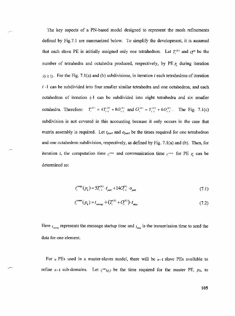
The key aspects of a PN-based model designed to represent the mesh refinements

defined by Fig.7.1 are summarized below. To simplify the development, it is assumed

that each slave PE is initially assigned only one tetrahedron. Let T/ k) and d,k) be the

number of tetrahedra and octahedra produced, respectively, by PE Jt during iteration

iCi ~ 1). For the Fig. 7.1 (a) and (b) subdivisions, in iteration i each tetrahedron ofiteration

i -1 can be subdivided into four smaller similar tetrahedra and one octahedron, and each

octahedron of iteration ~-1 can be subdivided into eight tetrahedra and six smaller

octahedra. Therefore: T(k) = 4T(k) + 80(k) and O(k) = T(k) + 60(k). The Fig. 7.1(c) 1 1-1 1-1 l ,-1 1-1

subdivision is not covered in this accounting because it only occurs in the case that

matrix assembly is required. Let (part and Opart be the times required for one tetrahedron

and one octahedron subdivision, respectively, as defined by Fig. 7.1(a) and (b). Then, for

iteration i, the computation time çmp and communication time çmm for PE Jt can be

determined as:

(7.1)

(7.2)

Here I"artul represents the message startup time and Idala

is the transmission time to send the

data for one element.

For n PEs used in a master-slaves model, there will be n-1 slave PEs available to

refine n-1 sub-domains. Let t,~(PO) be the time required for the master PE, Po, to

105

broadcast the sub-domain workload assignments to aIl slave PEso In total, n processors

will participate in the broadcast operation and the broadcast procedure will involve log(n)

point-to-point simple message transfers, with each transfer counting for a time cost of

tstartup + t data . (OH + Ti_ l ) [54]. Therefore, the total time that is required for one complete

procedure is

(7.3)

FinaIly, the overall time t, required to complete aH the mesh refinements for iteration i

will satisfy both (7.4) and (7.5), as se en from the timing chart presented in Fig. 7.3.

n-I

fi ~ ("""'(po) + max(fioomp(Pk)) + L(ticomm(Pk)) (7.4) k:1

= computation time = c o:m:munic ation time '1 ;:;;.

p~ ~C_-_-_""~~-~J~ __________ ~I---__ t~-~_-_=1~·_· __ "_~4j--~--~~. Il t/'"1V(P.) t/':'''!"'(Pj : ; 1 h j 1 1 : ; r •

l'"~-I-)!..-- rn"wl '--(P» • ~. .~J k

Figure 7.3: Timing for parallei mesh refinement in master-slaves model.

106

An individual module, named 'Co-Module', was developed for modeling the mesh

computation process, as shown in Fig. 7.4. The operation of the Co-Module procedure

starts with a scan of the tetrahedralloctahedral entities; then, the refinement rule is applied

to each individual tetrahedron/octahedron. Once an individual element is processed, a

signal is generated by Scan Trigger for loading the next geometrical entity.

The overall PN model development is shown schematically in Fig. 7.5. It involves six

modules, representing one master and five slave PEs, belonging to a symmetric


in the system, as indicated by Fig. 7.5. The system parameters tpart. 0part, tdata, and tstartup,

are each defined in the transition delays in each stage of the mesh refinement model. In

Fig. 7.5, the 'Co-Module' is abbreviated as a transition called "computation time".

t part

1 Tetrahedra

1

°8ta'lNrite Bock __ '----<

1

1

1

-----, 1 Geometry Scan Trigger: 1

1 T elrahedra 1 partlion"'\j Dono 1

P13

Octahedra 1

DataWrite 1 8ack 1

1

1 _J

Figure 7.4: The PN Co-Module: tetrahedron and octahedron sub-division.

107

1-" = QC

'"Ij

~. -....l V'I

~ ~ 3 o g. -8"' >-t

"0

[ -(1) -3 (1) tIl t:T" (il ::n ::s 3 a ~ §: tIl ~.

"'0 trl tIl

)

o

In~ialization

2

Receiving Tasks

Co- Module Computation Time

Co- Module Computation Time

Î

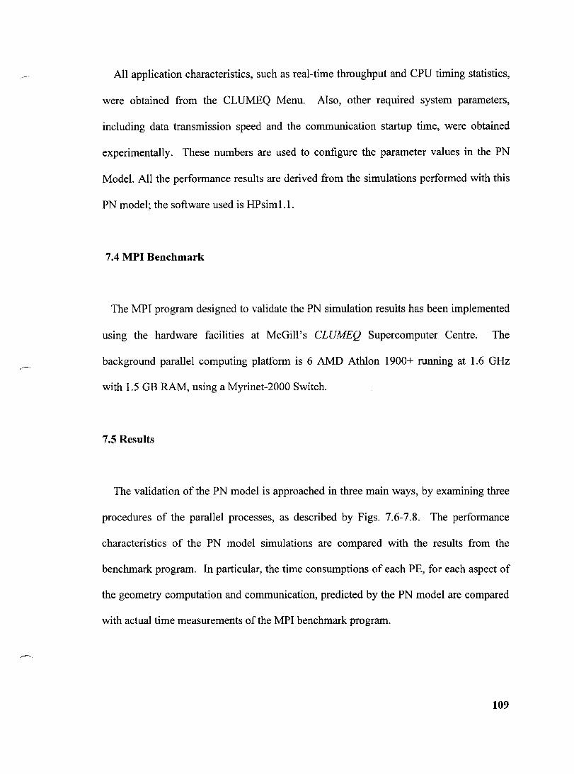
AlI application characteristics, such as real-time throughput and CPU timing statistics,

were obtained from the CLUMEQ Menu. AIso, other required system parameters,

including data transmission speed and the communication startup time, were obtained

experimentalIy. These numbers are used to configure the parameter values in the PN

Model. AlI the performance results are derived from the simulations performed with this

PN model; the software used is HPsiml.l.

7.4 MPI Benchmark

The MPI program designed to validate the PN simulation results has been implemented

using the hardware facilities at McGilI's CLUMEQ Supercomputer Centre. The

background parallei computing platform is 6 AMD Athlon 1900+ running at 1.6 GHz

with 1.5 GB RAM, using a Myrinet-2000 Switch.

7.5 Results

The validation of the PN model is approached in three main ways, by examining three

procedures of the parallel processes, as described by Figs. 7.6-7.8. The performance

characteristics of the PN model simulations are compared with the results from the

benchmark program. In particular, the time consumptions of each PE, for each aspect of

the geometry computation and communication, predicted by the PN model are compared

with actual time measurements of the MPI benchmark program.

109

The validation results for the mesh refinement computation performance for each PE in

the paraUel system are provided in Fig. 7.6. The master PE (0) does not have a mesh

computation workload; its dut y is to initiate slave PE processes at the start of each

iteration, and therefore the time costs of the master PE are approximately the same for

each iteration. Slave PEs 1 to 4 show similar computation times for each iteration since

their workloads are perfectly balanced. However, slave PE 5 was initiaUy assigned to

refine one octahedron, which is a larger workload than the other slave PEs, therefore its

time costs are higher.

The validation results for the data formatting processes are shown in Fig. 7.7. The

master and slave PEs work to write the result data into OFF files, to provide a graphical

file for each slave PE. During this phase of operations, the master PE will make every

slave PE wait until the master completes fixing an the coordinates offsets for an the

slaves; then the master win release an the slave PEs simultaneously. AH the PEs will

work synchronously in the system during this stage of operation.

The validation results for the data gathering processes are shown in Fig. 7.8. In this

stage, the master PE gathers data from each slave PE and writes out the final data file.

Each slave PE sends its data to the master PE asynchronously, and the master will wait

until the last communication is completed, usuaHy the last one is from PE 5 because PE 5

has the largest workload.

110

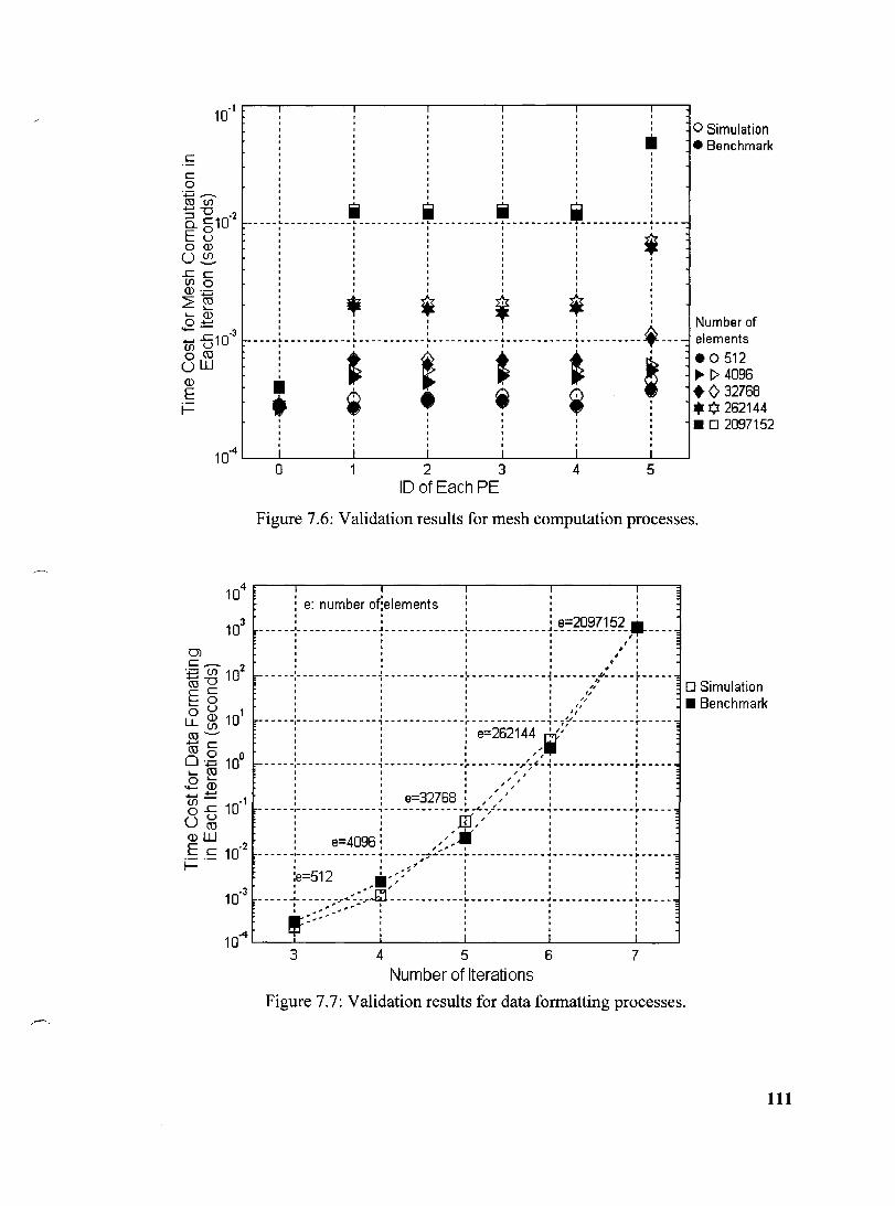
, 1 1. 1

: i i i ~ : _____ L ___________ ~-----------~-----------!-----------~ ___________ ~-----

$

: $

, ,

, , ,

• * 1 1 ~ 1 1

-----~-----------~-----------~-----------~-----------~----------~----, , • • ,

t ' ~ =

1 1 1 1 1

10.4 '-----'1 ____ ....... '1 ___ -'I ___ --'-I ___ -'I'--__ --LI_--' o 1 234 5

ID of Each PE

o Simulation .8enchmark

Number of elements

.0512 \III- t> 4096 +032768 • ô: 262144 .02097152

Figure 7.6: Validation results for mesh computation processes.

: : : : : e: number of:elements: : ,

: : : : e=2097152 .' ------:-------------~-------------~------------~------ ------, ----

1 1 lit 1

" . , . , . 1 1 1 1 # 1

............... _I ....................................... .! ...... __ ................ ___ 1 .............. __ ......... __ ... .! .................... 6 ............... !. ............ _ 1 1 1 1 JJ 1

l "'t 1 1 1", 1

, " 1 1 1,1

1 1 1 1 J, ............... -:- ................................. ~ ................................... -~ ......................... ~ .. fi'- ................... ~ ........ ...

: e=262144 '" : : ,i : 1 1 l '" 1 1

.......... -!-- ....................... ~ ..... -- .................. -~ ........ _ .... -r' .. " .. ~ .......................... ~ ........... -: 1 1 1 JI ,1' 1 1 ~ 1 1 1 JI '" 1 1 1 1 1 JI '" 1 1

: : e=32768: ,',': : .......... -:- ............................... ~ ... _ ... _ ..................... -"'r- ... ..c..~ ... ~.f_ ..................... ~_ ...... - --_ ... _ ...... - -~ - __ ... ...

1 1 m ~ 1

1 1 .l!.J ~ 1

: e=4096: /* : 1 1 ~,." 1 1 1 - _ ... - ... -:- - ........ - -- - ............ ~ ... - -- ... -~--:-... - -- -~ ... - - - -- - - - -- ... ~ .... - - ............. - - - i"" - _ ... 1 l ",'1 1 1 1

:e=512 .1 .. ~:"': : : 1 ,. '" 1 1 1 ..... _ .. .. _:- __ .. _ ........ ""' ... ---:...E:l- ....... -................... ~ __ ....... __ ........ __ ~ _ ... __ ..... __ .. _ ... _ ... ~ ___ .. ... f:::-=---- , , , ,

10·4~ __ J-________ L_ ______ ~ ________ ~ ________ ~~

3 456 Number of Iterati ons

7

Figure 7.7: Validation results for data formatting processes.

o Simulation .8enchmark

111

0).--. .2 e U') 10 'C "0 O)e

oC 0 ...... u roO) (.!)U')

ro ........... 10.3 ...... e roo 0'.;:::::; ,,-ro 0"..... 2 ...... - ·4 U') oC 10 Ou Uro O)W Ee i= ,- 10.5

~ ~ ~ ~ : : ~ ____ L ___________ L ___________ L ___________ ' ___________ l ___________ l ____ ~

"

: : : : .' 0 Simulation 1 1 1 1 : : : ! 1 :. 8enchmark : ! , , : :

----~----------~-----------~-----------!-----------!----------~---~ : : ~ ~ . : , ~ • T , , .' : : : : .' 1 1 1 1

-----r-----------~-----------~-----------~-----------~-----------T----~ , , , , , , , , , 1 1 1 1 1 1

----l----------t -----------t -----------1-----------1-----------1----~ Number of

i ~ * , ~ i elements : ' , , , ~. 0512

-----r --------- -t ---------t- ------ --t ---------t ---------~ ---~ : t ~~;~8 : : : : : :. Q 262144

.02097152 , , 10.6 l.----..JI'---__ ----1..I ____ I'---__ ----I.I ____ .L.." ___ --'1_-----'

o 1 2 3 4 5 ID of Each PE

Figure 7.8: Validation results for data gathering processes.

In summary, Figs. 7.6-7.8 all show close agreement between the timing results for the

PN model simulation (light symbols) and the corresponding MPI benchmarks (dark

symbols) for a series of five mesh refinement iterations. The small discrepancies

between the simulation and benchmark results may be due, in part, to the fact that the

potential effects of the processor cache is not accounted for in these PN model simulation

results.

7.6 Conclusion

A recently developed approach for modeling and simulating hierarchical tetrahedral-

octahedral mesh refinement in parallel has been validated using direct comparison with

measurements obtained from a prominent large-scale computing facility. The

112

comprehensive PN-based simulation model was implemented for the specifie HTO mesh

refinement algorithm under study, and the specifie computing architecture utilized at the

facility, in order to simulate the full functionality and runtime behavior of the combined

system. The HTO refinement algorithm was also implemented, according to the same

operating standards, for actual execution on the CLUMEQ supercomputer system. The

full series of primary comparative investigations examined confirm strong agreement

between the simulated performance results and the actual system performance results,

and together serve to validate the correctness of the PN modeling scheme. Further, as

indicated and illustrated by the model development and wide range of detailed simulation

results available, the PN approach has been demonstrated to be a versatile and powerful

modeling tool for producing realistic and detailed performance simulations for advanced

3-D FE mesh refinement algorithm implementations on large-scale parallel computing

facilities.

113

CHAPTER 8: Conclusion

8.1 Summary and Discussion

An effective modeling and simulation methodology is investigated for the performance

and computational complexity prediction in the design development and optimization of

3-D, parallel mesh refinement. The Petri Nets approach is proposed and evaluated as a

promising tool for describing and studying parallel meshing systems with properties of

being concurrent, parallel, and stochastic. This new mesh refinement simulation method

allows for a relatively detailed description of a system and can reveal key performance

characteristics in the parallel processes. The PN approach for modeling and simulating

the performance of the Random Polling Dynarnic Load Balancing protocol in parallel

Hierarchical Tetrahedral and Octahedral mesh refinement was applied. The efficiency

was exarnined by comparing the results with the algorithrn without a load balancing

mechanism.

New communication strategies were introduced for parallel mesh refinement that can

effectively overlap communication and computation operations to reduce inter-processor

communication blocks without compromising the load balancing. These are the

workload prediction approach and the task breaking point approach.

114

In the workload prediction approach, the workload is assigned to each slave PE by

predicting the consistency between each slave PE's local computation time and its result

data transmission time. The concept "load imbalance ratio" is introduced to de scribe the

workload difference between each slave PE, and it is the key parameter to pipeline the

computation time and communication time to make the slave PEs in the parallel system

communicate with the master PE one after another. Chapter 5 shows the improvement of

the speedup when workload prediction approach is applied to HTO mesh refinement.

The Task Break Point approach is fundamentally different from the workload

predication approach. The latter is based on pre-calculating and imposing systematic

workload imbalances across the processors to achieve the overlap. With the Task Break

Point scheme, the master PE is free to assign the workload for each slave PE according to

whatever net load balancing allocation is most appropriate. The master PE also specifies

a unique partitioning of each slave PE's total workload into a specific number of equal

length sub-task segments. This model ensures that each slave PE can receive a time

period of unobstructed communication with the master PE, immediately upon completion

of each sub-task. The Task Break Point pipelined communication can yield an average

speedup of ~ 10% compared to non-pipelined communication for large mesh refinement

in the resonant cavity case of chapter 6, and this speedup is in addition to the parallel

speedups.

The developed approach for modeling and simulating hierarchical tetrahedral

octahedral mesh refinement in parallel has been validated using direct comparison with

115

measurements obtained from a prominent large-scale computing facility. The

comprehensive PN-based simulation model was implemented for the specific HTO mesh

refinement algorithm under study, and the specific computing architecture utilized at the

facility and to simulate the full functionality and runtime behaviour of the combined

system. The HTO refinement algorithm was also implemented, according to the same

operating standards, for actual execution on the CLUMEQ supercomputer system. The

full series of primary comparative investigations examined confirms that there is a strong

agreement between the simulated performance results and the actual system performance

results. Together they serve to validate the PN modeling scheme. Further, as indicated

and illustrated by the model development and the wide range of detailed simulation

results available, the PN approach has been demonstrated to be a versatile and powerful

modeling tool for producing realistic and detailed performance simulations for advanced

3-D FE mesh refinement algorithm implementations on large-scale parallel computing

facilities.

8.2 Future Work

Future work should include utilizing Petri Nets for further performance optimization of

the computation and communication cost in parallel FEM mesh refinement algorithm for

systems of heterogeneous multiprocessors. Finally, the new modeling approach may be

extended to other aspects of the FEM, such as matrix assembly and solution methods.

116

REFERENCES

[1] Jianming Jin, The Finite Element Method in Electromagnetics, 2nd Edition,

Wi1ey-IEEE press, 2002.

[2] Nikos Chrisochoides, Andriy Fedorov, Bruce B. Lowekamp, Marcia Zangrill

and Craig Lee, "A case study of optimistic computing on the grid: paralle1 mesh

generation", Proceedings of the International ParaUel and Distributed

Processing Symposium (IPDPS'03), pp. 204-213, 2003.

[3] N. Chrisochoides, "A new approach to paralle1 mesh generation and partitioning

prob1ems", Computational Science, Mathematics and Software, pp. 335-359,

Purdue University Press, West Lafayette, USA, 2002.

[4] Y. Liu, H. Cheng, and C. King, "High performance computing on networks of

workstations through the exploitation of function paralle1ism", Journal of

Systems Architecture: the EUROMICRO Journal archive, Volume 45, Issue 15,

pp. 1307 -1321, 1999.

117

[5] Vladimir Zhulin, Steve Owen and Dale Ostergaard, "Finite element based

electrostatic-structural coupled analysis with automated mesh morphing" ,

Technical Proceedings of the 2000 International Conference on Modeling and

Simulation of Microsystems, pp. 501-504, San Diego, 2000.

[6] Roy D. Williams, "Performance of dynamic load balancing algorithms for

unstructured mesh calculations", Concurrency: Practice and Experience archive,

Volume 3, Issue 5, pp. 457 - 481, John Wiley and Sons Ltd., Chichester, UK,

1991.

[7] Kirk W. Cameron and Rong Ge, "Predicting and evaluating distributed

communication performance", Proceeding of the 2004 ACMlIEEE conference on

Supercomputing (SC 2004), pp.43-58, Pittsburgh, 2004.

[8] Y. Bi, S. Yang, and R. Smith, Distributed, Real-Time Systems: Monitoring,

Debugging, and Visualization, John Wiley & Sons, Inc., New York, 1996

[9] Jeffrey Tsai and T. Weigert, Knowledge-Based Software Development for Real

Time Distributed Systems, World Scientific Inc., New York, 1993.

[10] K. Erciyes, O. Ozkasap and N. Baykal, "A semi-distributed load balancing

model for parallel real-time systems", Informatica, Special Issue: ParaUel and

Distributed Real-lime Systems, Vol. 19-1, pp.97-109, 1995.

118

[11] A. Snavely, L. Carrington, N. Wolter, J. Labarta, R. Badia and A. Purkayastha,

"A framework for performance modeling and prediction", Proceedings of the

2002 ACMlIEEE conference on Supercomputing table of contents, pp 1 - 17,

Maryland 2002.

[12] L. Carrington, A. Snavely, N. Wolter and X. Gao, "A performance prediction

framework for scientific applications", Future Generation Computer Systems,

Volume 22, pp. 336-346, Elsevier Science, Amsterdam, 2006.

[13] Jennifer M. Schopf and Francine Berman "Performance Prediction in Production

Environments", 12th International ParaUel Processing Symposium & 9th

Symposium on ParaUel and Distributed Processing (IPPS/SPDP), pp. 647-653,

Orlando, 1998.

[14] Ruoming Jin, Ge Yang and G. Agrawal, "Shared memory parallelization of

data mining algorithms: techniques, programming interface, and performance",

IEEE Transactions on Knowledge and Data Engineering, Volume 17, Issue 1,

pp. 71- 89,2005.

[15] Y. Dallery, Z. Liu and D. Towsley, "Properties of Fork/Join queuing networks

with blocking under various operating mechanisms", IEEE Trans. on Robotics

and Automation, Vol. 13, No. 4, pp. 503-518, 1997.

119

[16] Wijesinghe, H. S., R. D. Homung, A. L. Garcia, and N. G. Hadjiconstantinou,

"Three-dimensional hybrid continuum-atomistic simulations for multiscale

hydrodynamics", Journal of Fluids Engineering, Number 126, pp. 768-777,

2004.

[17] P. Dinda, "Online Prediction of the Running Time of Tasks", Cluster Computing,

Volume 5, Number 3, 2002.

[18] S. Pllana and T. Fahringer, "Performance Prophet: A Performance Modeling and

Prediction Tooi for Parallel and Distributed Programs", The 2005 International

Conference ParaUel Processing, pp. 509- 516, 2005.

[19] Simone Sbaraglia, "the IBM high performance computing too1kit", IBM Petascale

Strategy Workshop, 2006.

[20] D.M. Rao and P. A. Wilsey, "Performance Prediction of Dynamic Component

Substitutions," Proceedings of the Winter Simulation Conference, pp. 816-824,

2002.

[21] AnyLogic 4.0 User Manual, URL: http://www.xjtek.comlproducts/anylogic/40.

[22] The Parsec Project, URL: http://www.parsec.org.

120

[23] Xiang Zeng, Rajive Bagrodia, and Mario Gerla, "GloMoSim: a Library for

Parallel Simulation of Large-scale Wireless Networks", Proceedings of the 12th

Workshop on Parallel and Distributed Simulations, pp.154-161, Banff, Canada,

1998.

[24] Connie U. Smith and Lloyd G. Williams, Performance Solutions: A Practical

Guide to Creating Responsive, Scalable Software, Addison-Wesley, 2001.

[25] D. Delamare, Y. Gardan and P. Moreaux, "Performance evaluation with

asynchronously decomposable SWN: implementation and case study",

Proceedings of lOth International Workshop on Petri Nets and Performance

Models, pp. 20- 29, 2003.

[26] J. Bradley, N. Dingle, P. Harrison and W. Knottenbelt, "Performance queries on

semi-Markov stochastic Petri nets with an extended continuous stochastic logic",

Proceeding of lOth International Workshop on Petri Nets and Performance

Models, pp. 62-71, 2003.

[27] M. Sereno, "Computational algorithms for product-form of competing Markov

chains", Proceedings of lOth International Workshop on Petri Nets and

Performance Models, pp. 93 - 102, 2003.

121

[28] Ajmone Marsan, M. Gribaudo and M. Sereno, "On Petri Net-based modeling

paradigms for the performance analysis of wireless Internet accesses",

Proceedings of 9th International Workshop on Petri Nets and Performance

Models, Page 19- 28, 2001.

[29] L. Wells, S. Christensen, L. Kristensen and K. Mortensen, "Simulation based

performance analysis of web servers ", Proceedings of 9th International

Workshop on Petri Nets and Performance Models, Page 59 - 68,2001.

[30] Peter MacNeice, Kevin M. OIson, Clark Mobarry, Rosalinda deFainchtein and

Charles Packer, "PARAMESH : A parallel adaptive mesh refinement community

toolkit.", Computer Physics Communications, vol. 126, p.330-354, 2000.

[31 ] J. Steensland, S. Chandra and M. Parashar, "An Application-Centric

Characterization of Domain-Based SFC Partitioners for ParaUel SAMR", IEEE

Transactions on Parallel and Distributed Systems archive, Volume 13, Issue

12, pp.1275 - 1289,2002.

[32] Ralf Deiterding, "AMROC, A generic framework for blockstructured Adaptive

Mesh Refinement in Object-oriented C++", URL: http://amroc.sourceforge.net.

[33] S. Crivelli and T. Head-Gordon, "A new load-balancing strategy for the solution

of dynamical large-tree-search problems using a hierarchical approach", IBM

122

Journal of Research and Development archive, Volume 48, Issue 2, pp. 153-

160,2004.

[34] X. Li and M. Parashar, "Hierarchical Partitioning Techniques for Structured

Adaptive Mesh Refinement Applications", Journal of Supercomputing, Kluwer

Academic Publishers, Vol. 28(3), pp.265-278, 2004.

[35] R. Hornung and S.R. Kohn, "Managing Application Complexity in the SAMRAI

Object-Oriented Framework," Concurrency and Computation: Practice and

Experience, Number 14, pp.347-368, 2002.

[36] R. Hornung, "AMR Application Development with the SAMRAI Library",

Workshop on Adaptive Mesh Refinement, LACSI Symposium, NM, 2004.

[37] Gunney, B., and A. Wissink, "Parallelizing the Point Clustering Algorithm in

Structured Adaptive Mesh Refinement," Presentation at 2005 SIAM CSE05

meeting, Orlando, FL , 2005.

[38] Shin'ichi Ezure, Hiroshi Okuda, Kengo Nakajima, "Parallel Mesh Relocator: A

Parallel Refining Software for Large-Scale Parallel FE Analysis", GeoFEM

Report Number 012,2002.

123

[39] J.P.Webb and S. McFee, "Nested Tetrahedral Finite Elements for h-Adaption",

IEEE Transactions on magnetics, Volume 35, Issue 3, pp.1338-1341, 1999.

[40] P. Jean Frey and P. L. George, Mesh Generation: application to jinite elements,

Hermes Science Publishing, Oxford, 2000.

[41] HPsim, URL: http://www.winpesim.de/petrinetlelhpsim_e.htm

[42] L. Oliker, R. Biswas and H. N. Gabow, "ParaUel tetrahedral mesh adaptation

with dynamic load balancing," ParaUe! Computing, vol. 26 (12), pp. 1583-1608,

2000.

[43] B.H.V. Topping, J. MuyUe, P. Ivanyi, R. Putanowicz and B. Cheng, Finite

Element Mesh Generation, Kippen: Saxe-Coburg, 2004.

[44] P. Sanders, "Asynchronous Random PoUing Dynamic Load Balancing", lOth

International Symposium on Aigorithms and Computation, pp. 37-48, 1999.

[45] K. Vip in, y. G. Ananth and R Venpaty, "Scalable load balancing techniques for

paraUel computers", Journal ofParaUel and Distributed Computing, Volume 22,

pp. 60-79, 1994.

124

[46] D. Q. Ren and D. D. Giannacopoulos, "A Preliminary Approach to Simulate

Parallel Mesh Refinement with Petri Nets for 3D Finite Element

Electromagnetics," Proceeding. of ANTEM 2004, pp.127-130, 2004.

[47] C. Girault and R. Valk, Petri Nets for Systems Engineering: A Guide to

Modeling, Verification, and Applications, Berlin:Springer-Verlag, 2002.

[48] C. Lindemann, Performance Modeling with Deterministic and Stochastic Petri

Nets, John Wiley & Sons Ltd., New York, 1998.

[49] G. Greiner and R. Grosso, "Hierarchical tetrahedral-octahedral subdivision for

volume visualization", The Visual Computer, Volume 16, pp. 357-369,2000.

[50] M.Dorica and D.Giannacopoulos, "Impact of mesh quality improvement systems

on the accuracy of adaptive finite element electromagnetics," IEEE Trans. on

Magnetics, Volume 41, Issue 5, pp, 1692-1695,2005.

[51] A. Grama, A. Gupta, G. Karypis and V. Kumar, Introduction to ParaUe!

Computing, second edition, New York: Addison Wesley Press, 2003.

[52] W. P. Petersen and P. Arbenz, Introduction to ParaUe! Computing: A Practical

Guide with Examples in C, Oxford: Oxford University Press, 2004.

125

[53] D. Q. Ren and D. D. Giannacopoulos, "Parallel mesh refinement for 3-D finite

element electromagnetics with tetrahedra: strategies for optimizing system

communication", IEEE Transactions on Magnetics, Volume 42, Issue 4, pp.

1251-1254,2006.

[54] Dennis D. Giannacopoulos and Da Qi Ren, "Analysis and Design of Parallel 3-D

Mesh Refinement Dynamic Load Balancing Aigorithms for Finite Element

Electromagnetics with Tetrahedra", IEEE Transactions on Magnetics, Volume

42, Issue 4, pp. 1235-1238,2006.

[55] Robert G. Sargent, "Verification and Validation of Simulation Models",

Proceedings of the 1998 Winter Simulation Conference, pp.121-130, 1998.

126

Documents

Analysis and Design Development ofParallel3-D Mesh ... · Analysis and Design Development ofParallel3-D Mesh Refinement Algorithms for Finite Element Electromagnetics with Tetrahedra