Embed Size (px)
Citation preview


Licentiate Thesis in Electrical Systems
Analysis and Control of a Hybrid
Vehicle Powered by a Free-Piston
Energy Converter
by
Jorgen Hansson
Electrical Machines and Power ElectronicsSchool of Electrical Engineering
Royal Institute of Technology (KTH)Stockholm, Sweden 2006
Submitted to the School of Electrical Engineering, KTH, in partialfulfillment of the requirements for the degree of Licentiate of
Engineering.

TRITA-EE 2006:047ISSN 1653–5146ISBN 91–7178–485–3
Elektriska Maskiner och EffektelektronikSkolan for Elektro- och Systemteknik, KTHTeknikringen 33SE-100 44 StockholmSweden
Copyright c© Jorgen Hansson, November 2006Printed by Universitetsservice US–AB

Abstract
The introduction of hybrid powertrains has made it possible to utiliseunconventional engines as primary power units in vehicles. The free-piston energy converter (FPEC) is such an engine. It is a combinationof a free-piston combustion engine and a linear electrical machine. Themain features of this configuration are high efficiency and a rapid tran-sient response.
In this thesis the free-piston energy converter as part of a hybridpowertrain is studied. One issue of the FPEC is the generation of pulsat-ing power due to the reciprocating motion of the translator. These pul-sations affect the components in the powertrain. However, it is shownthat these pulsations can be handled by a normal sized DC-link capac-itor bank. In addition, two approaches to reduce these pulsations aresuggested: the first approach is using generator force control and thesecond approach is based on phase-shifted operation of two FPEC units.The latter approach results in higher frequency and lower amplitude ofthe pulsations, which reduce the capacitor losses.
The FPEC start-up requirements are analysed and by choosing thecorrect amplitude of the generator force during start-up the energyconsumption can be minimised.
The performance gain of utilising the FPEC in a medium sized se-ries hybrid electric vehicle (SHEV) is also studied. An FPEC modelsuitable for vehicle simulation is developed and a series hybrid power-train, with the same performance as the Toyota Prius, is dimensionedand modelled.
Optimisation is utilised to find a lower limit on the SHEV’s fuelconsumption for a given drivecycle. In addition, three power manage-ment control strategies for the FPEC system are investigated: two load-following strategies using one and two FPEC units respectively and onestrategy based on the ideas of an equivalent consumption minimisation(ECM) proposed earlier in the literature.
The results show a significant decrease in fuel consumption, com-pared to a diesel-generator powered SHEV, just by replacing the diesel-generator with an FPEC. This result is improved even more by usingtwo FPEC units to generate the propulsion power, as this increases theefficiency at low loads. The ECM control strategy does not reduce thefuel consumption compared to the load-following strategies but gives abetter utilisation of the available power sources.
Keywords: free-piston energy converter, FPEC, series hybrid elec-tric vehicle, SHEV, power management, energy management, power-train evaluation, equivalent consumption minimisation, linear engine.


Preface
When I started this work, in December 2003, hybrid vehicles were nota common thing. Only a few models were available on the market andvery few were seen on the streets. On the other hand, one litre of gaso-line costed 9 SEK and no subsidisations for owning an environmentallyfriendly vehicle was available.
Today I often see hybrid vehicles driving in the city. In principleall large car manufacturers, which do not have a hybrid vehicle onthe market today, have announced that they will shortly. This risinginterest has been a great inspiration for me in my work.
Project History
The free-piston engine considered in this thesis has been investigatedfor quite some time now in Sweden. Sometime in 1996-97 a memberof the department of Mechanical Engineering, at the Royal Institute ofTechnology (KTH), contacted the department of Electrical Engineer-ing. He had an idea of combining a free-piston combustion engine witha linear electrical machine for generation of electric power. They in turnpresented the idea to ABB Corporate Research that also was interestedin investigating such a configuration.
In 1998 members from KTH and ABB visited Volvo Technology(VTEC) to discuss the idea. It turned out that VTEC already haddone a small study about such a machine but chosen not to go furtheras they believed that an electrical machine fulfilling the requirementsfor such an application would be too bulky.
Nevertheless, when the electrical engineers had convinced Volvo thatan electrical machine suitable for a free-piston engine could be devel-oped, they all decided to start a project under the name ”Fridolf”.The division, which nowadays has the name Combustion and Multi-phase Flow, at Chalmers University of Technology, was contacted forcombustion studies and funding was raised from the Swedish EnergyAgency.
In 2002 the Fridolf project turned into an European project withEU funding. Partners, both from university and industry in severalEuropean countries, then joined to develop a new technology with theaim to be efficient and suitable for vehicle propulsion, auxiliary powerunits and distributed generation. The result was a 45 kW free-pistonenergy converter (FPEC) prototype.
To complement this work two national projects funded by the SwedishEnergy Agency were initiated in 2003. One project at Chalmers thatis investigating homogenous charge compression ignition combustion infree-piston engines. The results so far from that project is presented in[19]. The other project has resulted in the work presented in this thesis.


Acknowledgement
This project is part of the Swedish Energy Agency (STEM) nationalresearch program ”Energisystem i Vagfordon”and the work presented inthis licentiate thesis has been made possible by their financial support,which is gratefully acknowledged.
During the years several people has contributed both to the workand to a good atmosphere at the division. I will, in no particular order,acknowledge them below.
First, I would like thank my supervisor Mats Leksell, for help,for support and for always taking the time to answer my questions.The two project leaders that have passed over the years, Peter The-lin and Fredrik Carlsson, are also acknowledged. Thanks to ChandurSadarangani for the interest in this project.
I would also like to acknowledge the external members of the refer-ence committee: Erland Max (VTEC), Hector Zelaya (ABB), MiriamBergman, Valeri Golovitchev, and Ingemar Denbratt (all three fromChalmers University of Technology). The committee meetings havebeen most fruitful to me, with interesting discussions around the FPECsystem.
Thanks to Jakob Fredriksson (Chalmers) who always has tried toanswer my combustion related questions, and to Martin West for up-dating us on the prototype’s control system.
The newsletter from Kaneheira Maruo has kept me updated on thedevelopments in the hybrid area around the world, which is acknowl-edged.
Special thanks goes to my roommate during the last two years, AlijaCosic, for joined laughter, for interesting discussions, for answering myquestions on electrical machines, and for always opening the windowon my demand.
When I started at the division I was ”raised” by Erik Nordlund andBjorn Allebrand to be a good PhD student the EME-way. Thanks forgiving me a good start.
I would like to thank the staff and my fellow PhD students at thedivision during the years for contributing to a relaxed work atmosphere.Thank you Janne, Stefan, Chandur, Mats, Fredrik, Hansi, Eva, Lennart,Sture, Olle, Emma, Robert, Tommy, Tomas, Dmitry, Bjorn, Erik, Syl-vain, Alija, Samer, Peter L, Peter T, Stephan, Florence, Mattias, Juli-ette, Mattias, Alexander, Henrik, Freddy, Karsten, Staffan, Hailian,Lilantha, Nicklas, and Torbjorn.
Finally, I would like to thank my family, Lennart, Karin and Nicklasand my girlfriend and ”in-laws” Malena, Bjorn and Eivi for their helpand support during the years.
Stockholm, November 2006Jorgen Hansson


Contents
Abstract i
Preface iii
Acknowledgement v
Contents vii
Notation xi
1 Introduction 11.1 Motivation and Scope of the Thesis . . . . . . . . . . . . 21.2 Contribution . . . . . . . . . . . . . . . . . . . . . . . . 31.3 Publications . . . . . . . . . . . . . . . . . . . . . . . . . 4
2 Free-Piston Engines 52.1 Components . . . . . . . . . . . . . . . . . . . . . . . . . 5
2.1.1 The Combustion Chamber . . . . . . . . . . . . . 62.1.2 The Rebound Device . . . . . . . . . . . . . . . . 62.1.3 The Load . . . . . . . . . . . . . . . . . . . . . . 6
2.2 The Free-Piston Energy Converter . . . . . . . . . . . . 62.2.1 Integrated Electrical Machine . . . . . . . . . . . 72.2.2 Free-piston Dynamics . . . . . . . . . . . . . . . 72.2.3 Resonant Behaviour . . . . . . . . . . . . . . . . 92.2.4 Low Mechanical Losses . . . . . . . . . . . . . . 92.2.5 Size, Weight and Robustness . . . . . . . . . . . 102.2.6 Efficient Combustion . . . . . . . . . . . . . . . . 10
2.3 Challenges . . . . . . . . . . . . . . . . . . . . . . . . . . 122.3.1 A Robust Electrical Machine . . . . . . . . . . . 122.3.2 Sophisticated Combustion Control . . . . . . . . 122.3.3 Elimination of Vibrations . . . . . . . . . . . . . 13
2.4 State of the Art . . . . . . . . . . . . . . . . . . . . . . . 132.4.1 The Free-Piston Energy Converter . . . . . . . . 132.4.2 The Linear Engine–Alternator . . . . . . . . . . 14
vii

2.4.3 The Free Piston Power Pack . . . . . . . . . . . 152.5 Suitable Applications . . . . . . . . . . . . . . . . . . . . 15
2.5.1 Primary Power Unit . . . . . . . . . . . . . . . . 152.5.2 Auxiliary Power Unit . . . . . . . . . . . . . . . 15
3 Hybrid concepts 173.1 Losses in a Vehicle . . . . . . . . . . . . . . . . . . . . . 183.2 Hybrid Topologies . . . . . . . . . . . . . . . . . . . . . 19
3.2.1 The Parallel Hybrid . . . . . . . . . . . . . . . . 193.2.2 The Series Hybrid . . . . . . . . . . . . . . . . . 203.2.3 Combined Configurations . . . . . . . . . . . . . 23
3.3 Commercial Hybrid Vehicles . . . . . . . . . . . . . . . . 243.4 Using the FPEC for Hybridisation . . . . . . . . . . . . 253.5 Conclusions . . . . . . . . . . . . . . . . . . . . . . . . . 25
4 Related Work 274.1 FPEC Models and Properties . . . . . . . . . . . . . . . 274.2 Propulsion Unit Configuration . . . . . . . . . . . . . . 284.3 Powertrain Evaluation . . . . . . . . . . . . . . . . . . . 294.4 Power Management . . . . . . . . . . . . . . . . . . . . . 29
5 FPEC Models 315.1 Cycle-to-cycle FPEC Model . . . . . . . . . . . . . . . . 31
5.1.1 Controller . . . . . . . . . . . . . . . . . . . . . . 315.2 Vehicle Simulation FPEC Model . . . . . . . . . . . . . 33
5.2.1 Efficiency Estimation . . . . . . . . . . . . . . . 335.2.2 Transient Response . . . . . . . . . . . . . . . . . 355.2.3 Start-up Requirements . . . . . . . . . . . . . . . 36
5.3 Conclusions . . . . . . . . . . . . . . . . . . . . . . . . . 39
6 Power Pulsations 416.1 Reduction by Force Control . . . . . . . . . . . . . . . . 42
6.1.1 Conclusions . . . . . . . . . . . . . . . . . . . . . 456.2 Reduction by Phase Shifted Operation . . . . . . . . . . 46
6.2.1 The DC-link Capacitor . . . . . . . . . . . . . . 476.2.2 Finding a Suitable DC-link . . . . . . . . . . . . 486.2.3 Conclusions . . . . . . . . . . . . . . . . . . . . . 49
7 Modelling of Vehicle Components 517.1 Vehicle Parameters . . . . . . . . . . . . . . . . . . . . . 527.2 Powertrain Components . . . . . . . . . . . . . . . . . . 53
7.2.1 Traction Electrical Machine . . . . . . . . . . . . 537.2.2 Gearbox . . . . . . . . . . . . . . . . . . . . . . . 557.2.3 Battery . . . . . . . . . . . . . . . . . . . . . . . 567.2.4 Power Electronics . . . . . . . . . . . . . . . . . 60
viii

7.2.5 DC-link . . . . . . . . . . . . . . . . . . . . . . . 60
7.2.6 Auxiliary Load . . . . . . . . . . . . . . . . . . . 61
7.2.7 Diesel Generator . . . . . . . . . . . . . . . . . . 61
7.3 Modelling for Optimisation . . . . . . . . . . . . . . . . 62
7.3.1 State-space Model . . . . . . . . . . . . . . . . . 63
7.3.2 Discretisation . . . . . . . . . . . . . . . . . . . . 64
7.4 Drive Cycle Analysis . . . . . . . . . . . . . . . . . . . . 64
8 Finding the Optimal Fuel Consumption 69
8.1 Linear programming . . . . . . . . . . . . . . . . . . . . 69
8.1.1 Cost Function . . . . . . . . . . . . . . . . . . . . 70
8.1.2 Constraints . . . . . . . . . . . . . . . . . . . . . 71
8.2 Implementation . . . . . . . . . . . . . . . . . . . . . . . 73
8.2.1 Optimisation Formulation . . . . . . . . . . . . . 74
8.2.2 Sample Time . . . . . . . . . . . . . . . . . . . . 74
8.3 Results and Conclusions . . . . . . . . . . . . . . . . . . 76
9 Power Management 79
9.1 Load Following Strategies . . . . . . . . . . . . . . . . . 80
9.2 The Equivalent Consumption Minimisation Strategy . . 82
9.2.1 The ECMS Cost Function . . . . . . . . . . . . . 83
9.3 The Algorithm . . . . . . . . . . . . . . . . . . . . . . . 84
9.3.1 Equivalent Discharge Consumption . . . . . . . . 85
9.3.2 Equivalent Charge Consumption . . . . . . . . . 86
9.3.3 The Equivalence Factor . . . . . . . . . . . . . . 87
9.3.4 Cost Function Analysis . . . . . . . . . . . . . . 88
9.3.5 Control Surface Calculation . . . . . . . . . . . . 89
9.3.6 Tuning of the Equivalence Factor . . . . . . . . . 91
9.4 Results and Conclusions . . . . . . . . . . . . . . . . . . 92
9.4.1 Behaviour . . . . . . . . . . . . . . . . . . . . . . 92
9.4.2 Battery Utilisation . . . . . . . . . . . . . . . . . 96
9.4.3 Fuel Consumption . . . . . . . . . . . . . . . . . 96
10 Conclusions and Future Work 99
10.1 The FPEC System . . . . . . . . . . . . . . . . . . . . . 99
10.2 Efficiency Estimation . . . . . . . . . . . . . . . . . . . . 100
10.3 Power Management . . . . . . . . . . . . . . . . . . . . . 100
10.4 Future Work . . . . . . . . . . . . . . . . . . . . . . . . 101
10.5 Conclusions . . . . . . . . . . . . . . . . . . . . . . . . . 102
A The Mass-Spring System 105
ix

B Longitudinal Vehicle Dynamics 109B.1 Vehicle Model . . . . . . . . . . . . . . . . . . . . . . . . 109
B.1.1 Aerodynamic Drag . . . . . . . . . . . . . . . . . 109B.1.2 Grading Resistance . . . . . . . . . . . . . . . . . 110B.1.3 Rolling Resistance . . . . . . . . . . . . . . . . . 110
B.2 Acceleration Parameters . . . . . . . . . . . . . . . . . . 110
Paper IMinimizing Power Pulsations in a Free Piston Energy Converter
Paper IIOperational Strategies for a Free Piston Energy Converter . . .
Paper IIIPerformance of a Series Hybrid Electric Vehicle with a FPEC .
References
x

Notation
Symbols
∆t Sample timeηch Battery charge efficiencyηdis Battery discharge efficiencyηconv Power converter efficiencyηgear Gearbox efficiencyηFP FPEC efficiencyn(i) Gear ratio n of gear iAf Vehicle frontal areaFel FPEC generator forceAp FPEC piston areaPbatt Battery powerPfuel Fuel powerPFP FPEC power
PFP FPEC power ratePFPref FPEC power referencePFPold Present FPEC power statePload Load powerPbr Brake chopper powerUDC DC-link voltageWbatt Battery energyWcond Capacitor energyWfuel Fuel energySoC Battery state-of-charge
Acronyms
APU Auxiliary Power UnitCI Compression IgnitedEGR Exhaust Gas RecirculationECMS Equivalent Consumption Minimisation StrategyEM Electrical MachineFPEC Free-Piston Energy ConverterHCCI Homogenous Charge Compression IgnitionHEV Hybrid Electric VehicleICE Internal Combustion EngineLP Linear ProgrammingPPU Primary Power UnitSHEV Series Hybrid Electric VehicleSI Spark IgnitedTDC Top Dead Centre
xi


Chapter 1
Introduction
The interest in hybrid electrical vehicles (HEV) and dual-fuel vehicleshas increased dramatically the last few years. These vehicles have po-tential to have lower emissions and fuel consumption than conventionalvehicles of the same size. However, the rising interest in these vehiclesis probably not a result of a sudden environmental awareness from ve-hicle customers. Instead, this interest may be explained by economicalfactors.
The rising oil price has made it somewhat more painful for peopleto refuel their vehicle, which has increased the demand for vehicleswith good fuel economy. Moreover, subsidisations and tax reductionshave made it more beneficial to buy and own these types of cars. Thisdevelopment came as a surprise to most car manufactures, but Toyotawas early with hybrid vehicles on the market and is dominating theHEV sales today.
Most hybrid vehicles have a drivetrain consisting of a conventionalinternal combustion engine (ICE) complemented in some way by anelectrical machine and an energy storage. As the ICE does not haveto provide all the propulsion power by itself, it can be utilised moreefficiently.
However, some hybrid solutions make it possible to rethink totallywhen it comes to the ICE. In the series hybrid topology the primarypower unit (PPU), which usually is an ICE, is only electrically coupledto the propelling electrical machine. As electrical power is required,and not mechanical torque like in a conventional vehicle, the use of arotating engine and generator is not the only solution.
A promising non-rotating alternative as PPU is the free-piston en-ergy converter (FPEC). The FPEC is a combination of a free-pistoncombustion engine and a linear electrical machine. The moving part inthis engine, the translator, has a reciprocating motion determined bythe forces acting on the piston and not by a crankshaft. This gives ben-
1

2 Chapter 1. Introduction
efits, both from combustion and mechanical points of view, resulting inhigh efficiency and a rapid transient response. In a project parallel tothis the prototype in Figure 1.1 has been built.
This type of energy converter has achieved increased attention dur-ing the last years. However, most published material focuses on mechan-ical design, electrical machine design, low-level control or combustion.Few results where entire FPEC systems are considered can be found.
Figure 1.1: The 45 kW prototype developed in the European FPECproject.
1.1 Motivation and Scope of the Thesis
The work in this thesis looks at the FPEC from a system perspective,that is, as part of a series hybrid drivesystem. The objectives are tostudy the FPEC related issues of such a system, to estimate the overallefficiency and to find suitable power management strategies.
Several models of free-piston engines have been presented earlier forexample in the parallel EU-project. However, all these models describethe FPEC dynamics and power output from cycle to cycle. For investi-gations on a larger time scale, for example, drive cycle simulations andpower management evaluations, another type of model is more suitable.Such a model is suggested in chapter 5.
The FPEC has properties that differ from conventional rotatingmachines and combustion engines. For example, the generated poweris pulsating due to the reciprocating motion of the translator. Thesepulsations affect the electrical part of the powertrain and the compo-nents must be dimensioned for this. In chapter 6 a DC-link capacitorbank that can handle these pulsations is dimensioned. In addition, two

1.2. Contribution 3
approaches that may reduce the influence of the pulsations are investi-gated.
To be able to analyse the FPEC system, a series electric hybridvehicle with same performance as the Toyota Prius is dimensioned andmodelled in chapter 7.
To get an efficient hybrid system, the available power sources mustbe controlled in a good way, hence, a good power management strategyis required. However, it is hard to know how good a strategy can bejust by doing simulations. Therefore, in chapter 8, linear optimisationis utilised to find a control independent benchmark value for the givenpowertrain and drivecycle.
The FPEC features make it suitable for load-following strategies butmany studies about series hybrid systems utilises on-off strategies forthe primary power unit. Power management strategies more suitablefor the FPEC system, and their influence on fuel consumption, areinvestigated in chapter 9.
1.2 Contribution
The work presented in this thesis extends the knowledge concerningseries hybrid systems with FPECs when it comes to:
• Generator force influence on system requirements.
• Ways to reduce the power pulsations.
• Energy and power requirements for FPEC start-up.
• FPEC models suitable for optimisation, high-level control evalu-ation and system simulation.
• Performance of an FPEC powered medium sized vehicle.
• Efficiency improvements by utilising several small FPEC modulesinstead of one large.
• Power management.

4 Chapter 1. Introduction
1.3 Publications
This work has, apart from this thesis, resulted in three publicationspresented at international conferences:
1. Minimizing Power Pulsations in a Free Piston EnergyConverterJorgen Hansson, Mats Leksell and Fredrik CarlssonProceedings of the 11th European Conference on Power Electron-ics and Applications (EPE05), Dresden, September 2005.
2. Operational Strategies for a Free Piston Energy ConverterJorgen Hansson, Mats Leksell, Fredrik Carlsson and ChandurSadaranganiProceedings of the Fifth International Symposium on Linear Drivesfor Industry Applications (LDIA2005), Kobe-Awaji, Japan,September 2005.
3. Performance of a Series Hybrid Electric Vehicle with a Free-Piston Energy ConverterJorgen Hansson and Mats LeksellProceedings of the 2006 IEEE Vehicle Power and PropulsionConference (VPPC06), Windsor, U.K., September 2006.

Chapter 2
Free-Piston Engines
Free-piston engines with internal combustion have been used success-fully in applications such as gasifiers, hydraulic pumps and compressorsfor more than 60 years. During recent years there has been a rising in-terest in combining the free-piston engine with a linear generator.
This chapter describes the functionality of free-piston engines ingeneral with emphasis on the dual piston type, which is the configu-ration used in the FPEC prototype. For a deeper review of free-pistonengines [15] is recommended.
2.1 Components
Independent of the intended application and configuration a free-pistonengine needs three fundamental components [15]: a combustion cham-ber, a rebound device (energy storing device) and a load (energy ab-sorbing device). These devices are coupled through a free-piston andthe interaction between the parts is what makes the free-piston enginework. A basic schematic view can be seen in Figure 2.1.
Combustionchamber
Rebound device
Load
Free Piston
Figure 2.1: Fundamental parts of a free-piston engine.
5

6 Chapter 2. Free-Piston Engines
Combustion chambers
Combustionchamber
Load
Combustion chamber
Dual piston typeOpposed piston typeSingle piston type
Load Load Load
Figure 2.2: Free-piston engine configurations.
Free-piston engines are usually classified based on the piston layoutsshown in Figure 2.2. Possible layouts are single piston, dual piston oropposed piston.
2.1.1 The Combustion Chamber
The energy is put into the system in form of fuel injected into the com-bustion chamber. Conventional combustion techniques such as sparkignition or diesel combustion have been used but lately there has beena rising interest to utilise Homogeneous Charge Compression Ignition(HCCI) due to the special properties of the free-piston engine.
2.1.2 The Rebound Device
To make the free piston reciprocate some kind of rebound device isrequired. This device stores part of the energy produced during theexpansion stroke and utilises it to force the translator to reverse itsdirection. The rebound device can for example be a gas spring or achamber where air is compressed.
2.1.3 The Load
Usually it is desirable to use the engine to produce or generate some-thing else but heat. It could for example be compression of air in acompressor, pressure to pump oil in a hydraulic application or gener-ation of electrical power. This useful energy is absorbed by the load,which can utilise the energy remaining after losses and storage in therebound device.
2.2 The Free-Piston Energy Converter
The free-piston engine considered in this thesis is of dual piston typeand a cross section is shown in Figure 2.3. It is working as follows.Two-stroke combustion in the chambers makes a translator, coveredwith magnets and with pistons at the ends, reciprocate. Thus, the re-bound device is alternate compression in the two combustion chambers.Electrical energy is generated by loading the translator with the linear

2.2. The Free-Piston Energy Converter 7
Exhaust valveIntake port
Fuel Injector
MagnetsStator winding
TranslatorPiston
Combustion chamber
Figure 2.3: Cross section of a free-piston energy converter.
electrical machine. This configuration has special properties and fea-tures that are described below.
2.2.1 Integrated Electrical Machine
Having an electrical machine integrated in the combustion engine givesa number of interesting features. The main purpose of the electrical ma-chines is of course to transform part of the translator’s kinetic energyinto electrical energy. It will also be used to stabilise the combustionprocess. Moreover, it can be used as a starter-motor to initiate the com-bustion process and for stop and emergency braking of the translator.In case of misfire it can provide additional power to the translator tocompensate for the lost combustion power.
2.2.2 Free-piston Dynamics
In the free-piston engine the motion is determined by the forces actingon the piston. If losses are neglected the piston motion is determined bythe pressure in each cylinder p1 and p2, and the force from the electricalmachine Fel. This can be described using Newton’s second law
mpd2x
dt2= p1(x)Ap − p2(x)Ap + Fel, (2.1)
where Ap is the piston top area and mp is the translator mass. From(2.1) it can be concluded that to affect the translator position x, ei-ther the force or the pressure must be adjusted. Furthermore, the onlything restraining the translator motion is the cylinder head, thus thecompression ratio is determined by the current force balance and canquite easily be varied.
In a crank engine, on the other hand, the piston trajectory is deter-mined by a slider-crank mechanism as shown in Figure 2.4. This resultsin a sinusoidal piston motion and a fixed peak compression ratio pre-determined by the pistons top position, the top dead centre (TDC).Furthermore, energy is stored in a flywheel, which evens out pulsationsand provides power during non-power strokes.

8 Chapter 2. Free-Piston Engines
Flywheel
Connecting rodCrankshaft
Cylinder
Piston
Figure 2.4: Components in a crankshaft engine. (Picture fromwww.wikipedia.org.)
0 10 20 30 40
−10
−5
0
5
10
15
20
Time [ms]
[cm
], [m
/s], [km
/s2]
Pos. [cm]
Vel. [m/s]
Acc. [km/s2]
Figure 2.5: FPEC translator position, speed and acceleration as func-tion of time.

2.2. The Free-Piston Energy Converter 9
In Figure 2.5 the motion of the FPEC translator is illustrated.As seen, the translator position over time is not sinusoidal as in thecrankshaft engine.
The translator’s reciprocating motion results in a pulsating gener-ated power. As no flywheel is present in a free-piston engine there is noeasy mechanical way to even out the pulsations. Instead, the electricalcounterpart to a flywheel, a capacitor, can be used. The pulsating poweris an important issue that affects the supply system and is discussedfurther in chapter 6.
2.2.3 Resonant Behaviour
A free-piston engine will behave almost like a mass-spring system, as thegas in the combustion chambers is acting like nonlinear springs. A mass-spring system reciprocates with a natural frequency and is preferablyoperated near, or at, this frequency as this requires the least additionalenergy.
If only pressure forces are considered, the reciprocating frequencyfFP of the translator can be approximated as
fFP ≈1
2π
√
2p0Apγ
mpL. (2.2)
The pressure p0 is the cylinder pressure when the translator is in themiddle, γ is the gas constant, Ap is the bore, L is the maximal strokelength and mp is the translator mass. A full derivation of (2.2) is givenin Appendix A.
The engine is operating in a two-stroke cycle, thus every stroke gen-erates power. Consequently, increasing the operating frequency resultsin an increased average output power. From (2.2) it can be concludedthat a low translator mass mp, short stroke length L or large bore Ap
are desired hardware properties if a high natural frequency should beachieved. However, the frequency is limited by the combustion process.To assure sufficient time for ignition, combustion and scavenging thereciprocating frequency cannot be too high.
2.2.4 Low Mechanical Losses
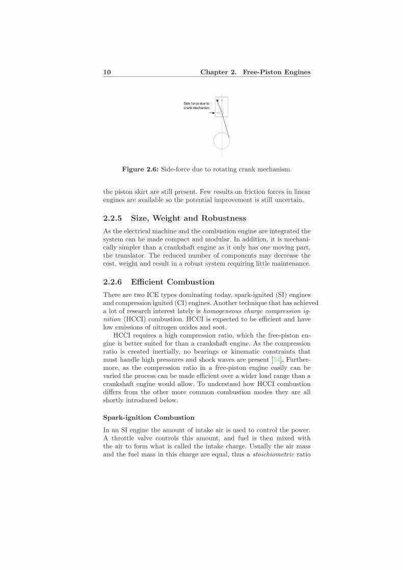
The reduced mechanical loss is one great benefit of the free-piston en-gine. As mentioned earlier, the engine has no slider-crank mechanism,flywheel or camshaft, and the friction loss is therefore expected to belower than in a crankshaft engine. In addition, a great source of loss,the piston side force originating from the crank mechanism, as seenin Figure 2.6, is reduced or eliminated due to the linear motion [25].Nevertheless, one of the main sources of friction, the piston rings and
10 Chapter 2. Free-Piston Engines
Side force due to
crank mechanisn.
Figure 2.6: Side-force due to rotating crank mechanism.
the piston skirt are still present. Few results on friction forces in linearengines are available so the potential improvement is still uncertain.
2.2.5 Size, Weight and Robustness
As the electrical machine and the combustion engine are integrated thesystem can be made compact and modular. In addition, it is mechani-cally simpler than a crankshaft engine as it only has one moving part,the translator. The reduced number of components may decrease thecost, weight and result in a robust system requiring little maintenance.
2.2.6 Efficient Combustion
There are two ICE types dominating today, spark-ignited (SI) enginesand compression ignited (CI) engines. Another technique that has achieveda lot of research interest lately is homogeneous charge compression ig-nition (HCCI) combustion. HCCI is expected to be efficient and havelow emissions of nitrogen oxides and soot.
HCCI requires a high compression ratio, which the free-piston en-gine is better suited for than a crankshaft engine. As the compressionratio is created inertially, no bearings or kinematic constraints thatmust handle high pressures and shock waves are present [54]. Further-more, as the compression ratio in a free-piston engine easily can bevaried the process can be made efficient over a wider load range than acrankshaft engine would allow. To understand how HCCI combustiondiffers from the other more common combustion modes they are allshortly introduced below.
Spark-ignition Combustion
In an SI engine the amount of intake air is used to control the power.A throttle valve controls this amount, and fuel is then mixed withthe air to form what is called the intake charge. Usually the air massand the fuel mass in this charge are equal, thus a stoichiometric ratio

2.2. The Free-Piston Energy Converter 11
is achieved. The intake charge is then compressed by the piston andignited by a spark plug. The fuel utilised should have a high octanenumber, that is, a high autoignition resistance. Premature autoignitionof the charge in an SI engine may result in a phenomenon called knockthat can damage the engine.
Compression Ignition Combustion
The CI engine compresses the intake air with the piston, until it ap-proaches its top position, the top dead centre (TDC). Fuel is theninjected and it ignites by itself as a result of the high pressure andtemperature in the combustion chamber. The amount of injected fuelis used to control the output power. In contrast to the fuel in the SI-engine, the fuel used here should have a high cetane number, whichmeans a high ability to autoignite under compression.
A CI engine has higher efficiency than an SI engine mainly for threereasons [52]:
The throttle valve present in the SI engine results in pump losses.As the CI engine does not have this component these losses areeliminated.
Higher compression ratio results in higher efficiency. An SI enginecannot have too high compression ratio as this may lead to knock.In a CI engine autoignition is desired and controlled, so the com-pression ratio is limited by other factors such as component strengthand heat loss.
Lower equivalence ratio which is the ratio of fuel over air. In an SIengine the amount of air mass over fuel mass is usually stoichio-metric as mentioned earlier, whereas the amount of fuel can bedecreased in a CI engine resulting in a lean charge.
Homogeneous Charge Compression Ignition combustion
An HCCI engine is compression ignited like a diesel engine, but thefuel is injected early in the stroke like in the SI engine. The fuel is thenmixed with air during the compression resulting in a nearly homoge-neous mixture. The mixture autoignites near the top dead centre andcombustion occurs almost simultaneously in the whole cylinder.
The heat release is very rapid and in a free-piston engine combustionclose to the ideal Otto cycle, that is, constant volume combustion, canbe achieved. This results in a high indicated1 efficiency. In addition, thealmost homogeneous mixture results in very low emissions of soot, and
1Also called thermal efficiency, a measurement on how well fuel is converted tomechanical work.

12 Chapter 2. Free-Piston Engines
a combustion temperature below 1800 K results in very low emissionsof nitrogen oxides.
However, during heavy loads the combustion temperature can goabove 1800 K. To prevent this, exhaust gas circulation (EGR) can beused, a technique common in diesel engines. As the name implies someof the already burnt exhaust gases are then recirculated into the com-bustion chamber (external EGR) or kept inside to the next cycle (in-ternal EGR). Mixing the charge with already burnt gas slows down thecombustion process and decreases the peak temperature.
However, the low temperature results in increased emissions of car-bon monoxide and unburned hydrocarbons. From an emission point ofview this can be handled by an oxidising catalyst. But as these emis-sions still contains chemical energy that is lost, the HCCI efficiency isstill reported to be close to the efficiency of conventional diesel com-bustion [19].
2.3 Challenges
The three challenges before a commercial free-piston engine with HCCIcombustion and a linear electrical machine for electric power generationwill be seen are discussed below. However, after the European FPECproject these issues do not seem impossible to solve.
2.3.1 A Robust Electrical Machine
The demands on the electrical machine used in this application arehigh. It should have a low specific weight and a high force density. Inaddition, it must work properly in a hostile environment and manageboth heat and vibrations.
Heat from losses in the electrical machine and from combustionmay expose the magnets on the translator to high temperatures. Asthe temperature increases the magnet flux starts to decrease and if thetemperature gets too high the magnets will be permanently demagne-tised.
However, investigations about this have been made in the FPECproject and FEM simulations indicate that the flux from the transla-tor magnets will be sufficient, even with temperatures as high as 100degrees at the translator ends.
2.3.2 Sophisticated Combustion Control
As the fuel is injected early in the stroke and ignites when the pressureand temperature are sufficient there exist no mechanical way, such as
2.4. State of the Art 13
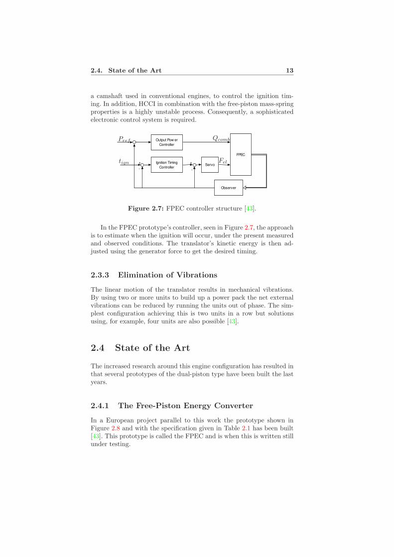
a camshaft used in conventional engines, to control the ignition tim-ing. In addition, HCCI in combination with the free-piston mass-springproperties is a highly unstable process. Consequently, a sophisticatedelectronic control system is required.
Output Pow er
Controller
Ignition Timing
Controller
Observer
FPEC
Servo+
-
+
-
Qcomb
Feltign
Pref
Figure 2.7: FPEC controller structure [43].
In the FPEC prototype’s controller, seen in Figure 2.7, the approachis to estimate when the ignition will occur, under the present measuredand observed conditions. The translator’s kinetic energy is then ad-justed using the generator force to get the desired timing.
2.3.3 Elimination of Vibrations
The linear motion of the translator results in mechanical vibrations.By using two or more units to build up a power pack the net externalvibrations can be reduced by running the units out of phase. The sim-plest configuration achieving this is two units in a row but solutionsusing, for example, four units are also possible [43].
2.4 State of the Art
The increased research around this engine configuration has resulted inthat several prototypes of the dual-piston type have been built the lastyears.
2.4.1 The Free-Piston Energy Converter
In a European project parallel to this work the prototype shown inFigure 2.8 and with the specification given in Table 2.1 has been built[43]. This prototype is called the FPEC and is when this is written stillunder testing.

14 Chapter 2. Free-Piston Engines
Figure 2.8: Prototype developed in FPEC project.
Table 2.1: Specification of the FPEC prototype.
Parameter ValuePeak power 45 kWPeak generator force 4 kNBore 102 mmTranslator mass 9 kg
2.4.2 The Linear Engine–Alternator
A group at West Virginia University has investigated, what theyrefer to as, a linear engine–alternator and two prototypes have beenbuilt. They have reported stable operation of a small spark-ignited lin-ear engine and an output of 316 W.
Figure 2.9: Second generation prototype from West Virginia Univer-sity [52].
Shown in Figure 2.9 is their second–generation prototype. A ma-chine with a bore of 76 mm and the possibility to vary the translatormass. An output of 2.8 kW with a translator mass of 2.8 kg and dieselcombustion has been reported [52]. Extensive computer simulations andparameter studies on both these engines have also been performed.

2.5. Suitable Applications 15
2.4.3 The Free Piston Power Pack
PEMPEK systems in Australia are suggesting a Free Piston PowerPack or FP3 as they call it [21]. The suggested power pack consists offour 25 kW FPECs integrated into one 100 kW unit as shown in Figure2.10.
Figure 2.10: The Free PistonPower Pack [8].
Figure 2.11: FP3 protoype [8].
One special feature of their concept is the integration of the com-pressor required for scavenging into the translator. Even though a fullprototype system appears to have been built no results seems to havebeen reported since 2003.
2.5 Suitable Applications
In this thesis the use of the FPEC as a primary power unit (PPU) isinvestigated. However, efficient power generation with low emissions isa desirable feature and several suitable applications can be proposed.
2.5.1 Primary Power Unit
A PPU is the primary source of power in a vehicle. The potential fea-tures of the FPEC making it appealing for vehicle applications are highefficiency over a large operational area, high power density, rapid tran-sient behaviour and low emissions.
2.5.2 Auxiliary Power Unit
An Auxiliary Power Unit (APU) is a selfcontained generator that couldbe used in for example, boats, trucks and tanks to provide electricityfor onboard systems. The FPEC’s compactness, modularity, efficiencyand low emissions make it suitable for such applications.

16 Chapter 2. Free-Piston Engines
A similar application is as a ”range extender” in an electric vehicle.The FPEC would then be used to charge the batteries when required,and not to provide the primary power. Hence, a lower power rating issufficient for that application. Moreover, the possibility to remove theFPEC from the vehicle when not needed could be implemented. Thiswould be desirable when, for example, going on shorter trips to thestore and more space in the vehicle is required.
Other possible applications could be as small power plants used forback-up power in hospitals, or for electrification of vacation cabins thatare not used all around the year.

Chapter 3
Hybrid concepts
In this chapter the benefits of hybridisation and the most commonhybrid topologies are presented.
A definition of a hybrid vehicle was given by the UN in 2003 [9]:
”A hybrid vehicle is a vehicle with at least two different energy convert-ers and two different energy storage systems (on-board the vehicle) forthe purpose of vehicle propulsion.”
But why is it beneficial to have ”at least two different energy con-verters”?
In a conventional vehicle the internal combustion engine has to pro-vide all the power and match the load at all times. The engine shouldtherefore ideally have high efficiency when the vehicle is starting, cruis-ing and accelerating. This is hard to fully achieve and as a result theaverage ICE efficiency is much lower than its peak efficiency. Moreover,when an ICE follows transient loads emissions may increase.
In a hybrid electric vehicle, however, one or more sources of powerare available and can support the ICE. This gives the possibility to op-erate the ICE more efficiently and avoid transients. In addition, mosthybrid systems have the ability to regenerate some of the vehicles ki-netic energy when decelerating, thus energy is regained ”for free” so tospeak. Furthermore, idling losses can be decreased or eliminated.
The main potentials of HEVs compared to conventional vehicles canbe summarised as
• Lower fuel consumption as a result of higher system efficiency.
• Lower fuel consumption as a result of energy regeneration.
• Lower emissions as a result lower fuel consumption and avoidanceof emission forming ICE transients.
17

18 Chapter 3. Hybrid concepts
These benefits are usually achieved without performance degradationsas electrical machines are good for propulsion.
3.1 Losses in a Vehicle
Approximately 15% of the fuel energy put into the tank of a conven-tional vehicle is used for propulsion and auxiliary loads; the rest is lostin the system. The typical energy distribution is shown in Figure 3.1.However, most if these losses can be reduced by hybridisation of thesystem. The loss numbers presented below are taken from [11].
Engine loss 62.4%Auxiliaries 2.2%
Idling 17.2%
Driveline 5.6%Propulsion 12.6%
Figure 3.1: Typical input energy distribution in a conventional vehicle[11].
Engine losses - 62.4%
A gasoline spark-ignited internal combustion engine has a peak effi-ciency of approximately 30% and diesel engine peaks around 40%. How-ever, in a conventional powertrain the ICE is not working at optimalworking points so much, which makes the average efficiency much lowerthan the peak efficiency.
By introducing additional power sources that can help the ICE, itcan be operated more frequently close to its peak efficiency. Moreover,the additional power source makes it possible to design ICEs that aremore efficient. For example, the ICE in the Toyota Prius is utilising theAtkinson cycle that has higher peak efficiency than a traditional en-gine. But at part load this ICE has lower efficiency than a conventionalengine. However, the overall system efficiency is not affected negativelyby this, as the electrical parts of the drivetrain are supporting the ICEduring these load levels.
Idling - 17.2%
When a vehicle with an ICE is at standstill, at red lights or in trafficjams for example, almost all of the energy is used to keep the enginerunning. These idling losses can be significantly reduced or eliminatedwith hybridisation.

3.2. Hybrid Topologies 19
In a parallel hybrid the combustion engine can be turned off atred lights as the electrical machine can rapidly start the engine andprovide the start torque. A series hybrid does not have to idle at all, asthe propulsion is pure electric. The series and parallel topology will bedescribed later on.
Transmission losses - 5.6 %
Hybridisation will not decrease the losses in the transmission as thesecomponents still are needed in a hybrid powertrain. However, develop-ment of more advanced transmissions in addition to improvement ofexisting technologies may improve the transmission performance in thefuture. Examples of advanced transmissions are the automated manualtransmission and the continuously variable transmission.
Auxiliary loads - 2.2%
The sub- and support systems in a vehicle requires energy. These sys-tems are for example, air conditioning, windshield wipers and powersteering. The trend seems to be that more and more electrical power isrequired on a vehicle. In a hybrid vehicle power from the high voltagesystem can be transformed to provide power for the auxiliary loads ifneeded.
3.2 Hybrid Topologies
Generally, hybrids are classified into two categories, depending on theconfiguration of the powertrain, series and parallel. Combinations ofthese configurations are also used, for example, in the Toyota Prius.
3.2.1 The Parallel Hybrid
In a parallel hybrid, a primary power unit (PPU) and an electric ma-chine (EM) are connected to the shaft through a transmission or clutchas seen in Figure 3.2. This makes it possible for the EM to provideadditional torque to complement the PPU when needed, for examplewhen starting from stand still or during heavy acceleration. The EMcan also be used for regeneration, charging of the energy storage, andfor pure electric propulsion. However, pure electric mode requires thatthe PPU is disengaged using the clutch. One drawback with this con-figuration is that if only one EM is present this EM cannot be used topropel the vehicle and charge the battery simultaneously. Moreover, asthe EM only delivers torque and cannot change the speed, the PPU’soperating point cannot be chosen to be fully optimal.

20 Chapter 3. Hybrid concepts
Electric
Motor/Generator
Energy
storage
DC/
AC
Gear-
box
Electric Power
Mechanical Power
ClutchPPU
Figure 3.2: Parallel hybrid topology.
If the clutch is removed and the EM is placed directly on the drive-shaft the configuration is usually called an integrated starter generator(ISG) system. The power rating of the EM in such a system is usuallyquite low.
Figure 3.3: The Honda IMA system, a 1.0 litre 3-cylinder gasoline di-rect injection engine combined with a 10 kW electric motor/generator.
Honda has developed a parallel system they refer to as the IntegratedMotor Assist (IMA). One example of their system is given in Figure3.3.
3.2.2 The Series Hybrid
In the series hybrid electric vehicle (SHEV), electrical power is gen-erated by a PPU driving a generator as shown in Figure 3.4. As thePPU must generate electrical power, alternatives for electricity gener-ation, besides a common ICE-generator combination, are fuel cells orthe FPEC.
Nevertheless, the generated power in combination with power fromthe energy storage is used by the propelling EM. Thus, the PPU doesnot have to be rated for the peak traction power as the energy storagecan assist.

3.2. Hybrid Topologies 21
The energy storage can be recharged with power either from thePPU or from regeneration when breaking. As the PPU is mechanicallydecoupled from the driveshaft its operating points can be chosen in-dependent of the required torque and speed of the vehicle. Thus, theefficiency may be increased. In addition, it can be located at a suitableplace in the vehicle body as only electrical connections are required.
Generator
Electric
Motor/Generator
DC-
linkDC/
AC
DC/
DC
AC/
DCPPU
Energy
storage
Electric Power
Mechanical Power
Figure 3.4: Series hybrid topology.
Drawbacks usually mentioned for the SHEV are the many powerconversions and that the traction EM must be sized for the total trac-tion power.
There is to my knowledge no commercial available series hybridtoday. However, the Orion VII series electric hybrid busses, shown inFigure 3.5, are currently being tested in New York. These busses haveachieved up to 45 % better fuel economy than a diesel bus [1]. In ad-dition, they are appreciated by the drivers due to the increased torqueoutput.
Figure 3.5: Orion VII series electric hybrid bus [1]
Furthermore, BAE Systems Hagglunds AB are developing a modulararmoured tactical system, seen in Figure 3.6, with the abbreviation SEP.This vehicle is an SHEV powered by diesel generators and with a totaltraction power of 100kW. It is propelled by electric motors integratedin the wheel hubs [1].

22 Chapter 3. Hybrid concepts
Figure 3.6: BAE systems ”Splitterskyddad Enhetsplatform” SEP [1].
If the PPU and generator are removed the result is a pure electricvehicle. One interesting electric vehicle reaching the market in 2007 isthe Tesla Roadster from Tesla Motors [13] seen in Figure 3.7. It hasquite impressive performance as seen in Table 3.1 but also a price tagof $100 000.
Figure 3.7: The Tesla Roadster [13].
Table 3.1: Performance of the Tesla Roadster.
Parameter DataAcceleration 0-100 km/h 4 sTop speed 210 km/hRange 150 kmBattery Lithium-IonInduction Machine peak power 135 kW@13500rpmGears 2-speed electric shift

3.2. Hybrid Topologies 23
3.2.3 Combined Configurations
Topologies that cannot be categorised as series or parallel drivetrainsalso exists and two such configurations will be described here. However,others may already exist or be developed in the future.
The Series-Parallel Configuration
In the Toyota Prius and Ford Escape for example, a configuration thatis a combination of the series and parallel system is used. The topologyis shown in Figure 3.8 and as seen it utilises two electrical machines.One is connected to the drive shaft like in the parallel topology. Thatelectric motor is used to provide additional traction power to the wheelsusing power from the PPU or the energy storage. It can also be usedfor pure electric propulsion and for regeneration of energy. The otheris a generator used to convert the ICE power to electrical power. The
Energy
storage
AC/
DC
Gear-
box
Electric
Motor/Generator
Electric Power
Mechanical Power
ICEPower
split
Generator
Figure 3.8: Series parallel topology.
key component in this system is the power split device, which is aplanetary gear in the Prius. It is connected to the generator, the ICEand the driveshaft, and controls the direction of the powerflow.
A similar concept to this, with the name two-mode hybrid, is an-nounced by the hybrid alliance between BMW group, DaimlerChryslerAG and General Motors [3].
The Four-Quadrant Transducer
The Four-Quadrant Transducer (4QT) system shown in Figure 3.9 isworking like an electrical gearbox with the ability to add and reducepower from the drive shaft. This ability and the two electrical machinesmake it possible to adapt both the speed and the torque of the ICEto the torque and speed needed for propulsion. Hence, the ICE can beoperated more efficiently. The two electrical machines are preferably

24 Chapter 3. Hybrid concepts
EM1
AC/
DC
ICE
Energy storage
Electric Power
Mechanical Power
EM2
AC/
DC
Figure 3.9: The 4QT system.
integrated into one double-rotor machine to reduce the system size andweight. The 4QT system can regenerate energy and a pure electric modeis possible if the electrical machines can deliver sufficient power.
3.3 Commercial Hybrid Vehicles
The last year a number of hybrid vehicles have been released on themarket and more are expected. Examples of hybrid vehicles that canbe bought today are given in Table 3.2.
Table 3.2: Examples of hybrid vehicles available on the market 2006.
Manufacturer Model Hybrid typeToyota
Highlander Series-parallelLexus RX400h Series-parallelPrius Series-parallel
HondaAccord ParallelCivic ParallelInsight Parallel
FordEscape Series-parallel
Toyota are today dominating the market, of approximately 200 000sold hybrids in the U.S. in 2005, 70 % were Toyota vehicles and theToyota Prius was the best selling model with 100 000 units sold inthe U.S.[12]. Honda is in second place with 20 % of the U.S market.However, most other manufacturers have not released their hybrid al-ternatives yet, but as mentioned earlier they have announced releases.

3.4. Using the FPEC for Hybridisation 25
3.4 Using the FPEC for Hybridisation
So why should an FPEC be used in hybrid vehicle? As the FPECgenerates electrical power it must be used in a series hybrid system.Most series systems so far utilises a conventional ICE combined witha generator; both the Orion bus and the SEP mentioned earlier havethat solution. However, an FPEC system has the following potentialadvantages over such a diesel-generator system:
Higher efficiency. The FPEC is expected to have approximately 45%peak efficiency from fuel to electricity, whereas a diesel-generatorhas around 38%. The other components in the system are essen-tially the same. Nevertheless, the total FPEC system efficiencywill probably be higher than for other series systems due to theincreased PPU efficiency.
Rapid transient response. HCCI and the free-piston dynamics re-sults in an ability to change between load levels very fast. Thistransient behaviour is usually undesirable when conventional ICEsare used as emissions then may increase. Furthermore, the FPEChas high efficiency over a wide load range whereas an ICE usuallyhas a peak. These two features make it possible to have a fairlysmall complementing energy storage. On the other hand, to utiliseregenerated energy in a good way the energy storage cannot betoo small.
Lower emissions. HCCI combustion in combination with an oxidis-ing catalyst will result in very low emissions.
Cylinder deactivation. An FPEC system will probably be realisedusing two or more FPEC units to reduce vibrations and electricpulsations. In such a configuration it is possible to shut down someunits when the load demand is low. This forces the still activeunits to operate at a higher load level and thus higher efficiency.A similar procedure has been used, in large crankshaft-engines,under the name cylinder deactivation.
3.5 Conclusions
In this chapter an overview over the most common hybrid topologieswas given. As discussed, several benefits can be achieved by hybridisinga powertrain.
On the other hand, hybridisation introduces some issues. For ex-ample, a hybrid powertrain is more complex than a conventional pow-ertrain, as components such as power electronics, battery packs and

26 Chapter 3. Hybrid concepts
electrical machines are required. Some of these components are quiteexpensive and, in addition, an increased number of components mayincrease the risk for failure. Furthermore, if hybrid vehicles becomemore common, car repair shops must gain the capability to handle theelectrical drivesystem.
Nevertheless, the hybrid technology is one way to reduce the fuelconsumption and lower the emissions of vehicles. But it still has to beseen if it is the way that the car manufacturers will choose.

Chapter 4
Related Work
The combination of a free-piston engine and a linear electrical machinehas gained increased research interest the last years. Published stud-ies are covering areas such as electrical machine design, low-level con-trol, combustion, and parameter studies. However, few studies on entireFPEC systems and FPEC related issues are available. Thus, these areareas requiring more attention. Modelling, analysis and control of hy-brid vehicles, on the other hand, are presently quite popular researchareas and large number of studies can be found.
4.1 FPEC Models and Properties
Several mathematical models of free-piston energy converters have beenpresented. For example, a model suitable for combustion investigations[27] and a model, including combustion, translator dynamics and losses,used for parameters studies [16]. In the FPEC project, a model for theinitial studies and controller design has been developed. This modelwas, for example, used in [25] and is discussed more in chapter 5.
However, the above mentioned models describe the FPEC dynam-ics from cycle to cycle. When doing quasi-stationary vehicle simula-tions a model describing the average power output over several cyclesis sufficient. Using the above models, for such investigations, results inunnecessary long simulation times.
One feature of the FPEC is the use of the integrated electrical ma-chine as a starter motor. However, the requirements for such a proce-dure are so far uninvestigated. The electrical machine can also be usedto stop the translator; both for regular engine shutdown and in caseof system faults. By using the electrical machine it is possible to stopthe translator within 40 % of the total stroke length [56]. However, thisrequires that the machine is used actively. Just using a resistive load
27

28 Chapter 4. Related Work
on the electrical machine does not give sufficient force to fully retardthe translator in less than one stroke when it is operating at ratedconditions [56].
Furthermore, by suitable control of the generator force it may bepossible to reach secondary goals besides combustion stabilisation, forexample pulsation reduction. Another goal could be high electrical ma-chine efficiency, which can be achieved by having speed and force pro-files that match [38].
The translator velocity, on the other hand, is hard to influence asit is almost totally determined by the combustion forces. In fact, acomplex shape of the force profile is required to influence the almostresonant translator motion [16].
4.2 Propulsion Unit Configuration
Internal combustion engines usually have lower efficiency at low loads.Cylinder deactivation is one approach utilised in large crankshaft en-gines to increase the part load efficiency [10]. A number of cylinders arethen deactivated when the power demand is low, temporarily turning,for example, a V8 into a V4.
A similar efficiency increase can also be achieved in an FPEC systemby building a propulsion unit using several small units instead of onelarge. The number of active units should then be determined by theload power to assure that each active unit is operating at a fairly highload level and thus, high efficiency.
The total volume of the FPEC system may be decreased by usingseveral smaller units. The first-order analysis presented in [21] suggeststhat when the engine is scaled the relationship between power changedue to scaling dP , and the volume change dV is described by
dP = dV (2/3). (4.1)
This indicates that building an FPEC propulsion unit using two FPECs,instead of one large, results in that the two-FPEC unit has only 70 % ofthe volume occupied by the one-FPEC unit. The total output power ofthe propulsion units are the same. However, the analysis in [21] makesmany simplifications and does not consider secondary effects.
Other benefits can also be achieved. Mechanical vibrations can bereduced by running the units out of phase [43] or the power pulsationamplitude can be decreased and the reciprocating frequency increased,as suggested in chapter 6.

4.3. Powertrain Evaluation 29
4.3 Powertrain Evaluation
When a powertrain or a control algorithm is developed it must be eval-uated. One common way for evaluation is utilisation of simulation mod-els. However, it is hard to know how good the powertrain can be justby doing simulations. In addition, when simulating a hybrid power-train a control law deciding the powerflow is usually required and thepowertrain’s final performance is very dependent on this control law.
To achieve results that do not depend on how the control law isdesigned, many recent studies suggest optimisation as a tool for pow-ertrain evaluation. By choosing powerflow as optimisation variable, theresult is independent of the control law. In addition, the controllershould often minimise objectives, such as fuel consumption, driveabil-ity or emissions, under system constraints. Constraints can easily beincluded in an optimisation formulation.
The most common optimisation method seems to be dynamic pro-gramming, which is utilised in several studies, for example [20, 34].However, one major drawback of dynamic programming is the curseof dimensionality. As both time and state-space must be discretised,to solve the problem numerically, the number of optimisation variablesmay be quite large. This number grows fast when additional states areincluded or a long time is to be studied.
Other suggested approaches are quadratic programming and linearprogramming. In [51], linear programming is used to find the lowest fuelconsumption for a small SHEV. The fuel consumption map is approx-imated by a piecewise linear function, and everything else is approxi-mated with linear functions. The optimisation result is used to find afigure of merit for causal controllers.
Combining a simulation model and a search method has also beensuggested [28]. However, these methods usually have nonlinear problemformulations resulting in that local optimums are found. Thus, they aremore suitable for finding suitable starting values for parameters thanfor evaluating the best performance of a powertrain.
4.4 Power Management
As mentioned earlier, a hybrid vehicle requires a power managementstrategy. In the literature the term energy management is also com-monly used, but as it is flow, and thus power, that is controlled theterm power management is used in this thesis. Nevertheless, this strat-egy is not required in a conventional vehicle as the only source of poweris the ICE. The redundancy of power sources in a hybrid, however, re-quires a systematic way to decide how the power should flow in thepowertrain and which power sources to utilise.

30 Chapter 4. Related Work
The raising interest in hybrid vehicles is also reflected in the increas-ing number of published power management investigations. One trendseems to be that older publications often have the SHEV as the in-tended application for the strategy, whereas parallel and series-paralleltopologies are common in more recent publications. This is probablyjust a reflection of the commercially available topologies.
For series hybrid vehicles two power management strategies are com-mon in the literature. The first one appears under several names: On-Off, Thermostat or Duty-Cycle strategy [18, 31]. This type of strategyutilises the primary power unit (PPU), operating at a working pointwith high efficiency, to recharge the battery to an upper limit when thestate-of-charge has reached a lower limit. In addition, the PPU pro-vides extra power to the wheels when the load is high. Some advancedvariants estimate the average mean traction load, and provides thataverage power by duty-cycle the PPU [17].
The second type of strategy is the load-following strategy [33], wherethe PPU follows the power load demand, usually with a rate-of-changelimit. The PPU’s working point having the highest efficiency for thecurrent power demand is preferably chosen. The power difference be-tween the PPU and the load, due to the rate-of-change limit, is providedby the energy storage.
Strategies similar to the above described have been investigated in[36] by simulation of a heavy-duty truck powered by an FPEC. Theload-following approach seems to have the greatest potential and upto 25 % lower fuel consumption than a conventional truck is reported.However, that result is achieved with an assumed FPEC efficiency thatpeaks above 50 %, which may be optimistic.
Even though a load-following strategy suits the FPEC, such a strat-egy requires optimisation of start and stop thresholds to achieve re-ally good performance. A more systematic approach to decide how thepower sources on a hybrid vehicle should be utilised is desirable.
The equivalent consumption minimisation strategy (ECMS) is a newpromising theory. It controls the power flow so an equivalent energycost is minimised each time step. The earliest published appearanceof a method of this type seems in the paper by [46]. Variations ofthe strategy have been presented since then and some versions havesuccessfully been used on real vehicle applications [47].

Chapter 5
FPEC Models
For the investigations in this thesis different types of FPEC models arerequired. The pulsation study in chapter 6 requires a dynamic FPECmodel describing every stroke and combustion. However, for the opti-misation in chapter 8 and the power management studies in chapter 9,it is sufficient with a simplified model. A drive cycle is usually severalminutes long and when internal FPEC dynamics are not to be stud-ied a model describing the FPEC properties on a higher level is moresuitable.
This chapter describes both an FPEC model available from the par-allel EU-project and the development of an FPEC model more suitablefor drive cycle simulations.
5.1 Cycle-to-cycle FPEC Model
An FPEC model has been developed in the parallel EU project, mainlyby Dr. Erland Max, for investigations of FPEC control, dynamics andparameters. This model, seen in Figure 5.1, is described in the thesis[25] and in the appended paper [29]. It is therefore not described indetail here. In general it can be said that the model is constructed bya combination of thermodynamic laws to describe pressure and tem-perature variations, ignition and heat release models for combustionand Newton’s second law for translator dynamics. This model will bereferred to as the EU-model.
5.1.1 Controller
The version of the EU-model used in this thesis does not have thekinetic energy controller described in section 2.3. Instead it utilises an
31

32 Chapter 5. FPEC Models
Project: FPEC, G3RD−CT−2002−00814Subject: Basic simulations 4.Work package: WP2−6.Erland Max, VTEC, 2003−03−31.
FPECFPEC_Engine_4
v xforce acc
Combustion force
4
p_cylinders
3
acceleration
2
position
1
P_el
1s
v
xvalves
valves_2
v
xvalves
valves_1
1s
p_diff
x injection
injection_2
x injection
injection_1
Vol, S
v_mean
valves
dQ/dt
p
T
cylinder_2
Vol, S
v_mean
valves
dQ/dt
p
T
cylinder_1
x Vol, s
Volume−Surface_2
x Vol, s
Volume−Surface_1
Mux
v_mean
F_el
T1
p1
a
T2
p2
x
F_fric
Q_comb
freq
v
[el_eff]
[F_el]
[p1]
[p2]
[a]
[x]
[v_mean]
[v_mean]
[v]
[x]
[v]
v
p2
p1
F
FrictionA_p
F_diff
v
x
F_el_request
F_el_output
Electrical machineEl_force
−1
injection
p
T
Q_comb.
dQ/dt
Combustion_2
injection
p
T
Q_comb.
dQ/dt
Combustion_1
1/m
P_el
v
x
v_mean
freq
v_mean computations
2
F_el_req
1
Q_combustion
Combustion force
"Electrical" force
Friction force
Figure 5.1: FPEC simulation model.
event triggered PI-controller. For decoupling a matrix with values froma relative gain array (RGA) analysis is used.
FPEC
-
Deco
uplin
g
PI-controller
PI-controller
Qcomb
Fel
tignref
Pref
tign
Pout
Figure 5.2: EU-model controller structure.
An illustration of the controller structure is shown in Figure 5.2.The controlled variables are output power Pout and ignition timingtign. They are controlled using electrical machine force Fel and fuelenergy Qcomb as control signals. This controller was developed in theearly stages of the European FPEC project and it is working as follows:
1. When the pressure in a combustion chamber reaches its peakvalue, over a combustion cycle, a trigger signal is sent to the con-troller, thus the controller is triggered once each stroke.

5.2. Vehicle Simulation FPEC Model 33
2. The PI-controllers controls ignition timing tign and the averageoutput power Pout. Each time they are triggered new output val-ues are sent to the decoupling block.
3. The FPEC is a multivariable system and the output signals Pout
and tign depends on both Qcomb and Fel. The decoupling blocktries to reduce this cross coupling. This is achieved by using amatrix with values determined from an RGA analysis. More in-formation about this method can be found in most textbooks onmultivariable control theory.
4. After decoupling suitable values for Qcomb and Fel are sent asinputs to the FPEC.
It should be noted that this controller was already given and is notpart of the work in this thesis. However, the performance is satisfactoryfor the investigations in this thesis where the EU-model is utilised.
5.2 Vehicle Simulation FPEC Model
The EU-model is suitable when studying dynamic properties and pa-rameters of the FPEC. However, for fuel consumption and power man-agement investigations, based on drive cycles that are several minutes,it is not necessary to have a dynamic model describing the pressurechanges and power output for each stroke. Instead, to decrease thesimulation time, a high-level FPEC model describing the power out-put averaged over several cycles is desirable. Such a model should alsocapture the following properties:
• The fuel consumption or efficiency of the engine.
• The transient response, that is, how fast the engine can changeits operating point and how it behaves during the change.
• Start-up time and power consumed during start-up.
This type of model was not available and has to be developed for thiswork. An estimation of the transient response can be obtained directlyfrom the EU-model whereas a modification of the model is requiredto get a proper efficiency estimation. The start-up requirements areinvestigated in a study of its own.
5.2.1 Efficiency Estimation
The EU-model considers losses from heat transfer, friction and a non-ideal thermodynamic cycle. These losses are important from combus-tion and mechanical point of view, however, no losses due to the conver-sion from mechanical to electrical power are considered. The EU-model

34 Chapter 5. FPEC Models
is therefore extended with the efficiency map shown in Figure 5.3 de-scribing the electrical machine and the rectifier efficiency.
Figure 5.3: Efficiency map for the FPEC’s electrical machine andpower converter [55].
In addition, the FPEC system requires a compressor for scavenging.A compressor consumes power and consequently decreases the systemefficiency. In conventional engines the power consumption of compres-sors used for turbo or super charging is dependent on the engine speed.In the FPEC, however, the frequency is almost constant over the loadrange and the compressor power consumption will consequently notvary much. A constant consumption of 1 kW over the entire load rangeis therefore assumed.
An estimation of the efficiency, from fuel to electrical power, asfunction of load power can now be achieved by simulating the modifiedEU-model with output power from 1 kW to 45 kW.
0 10 20 30 400
0.1
0.2
0.3
0.4
Load power [kW]
Effic
iency
Figure 5.4: Conversion efficiency from fuel to electrical power. Thethick line is the FPEC efficiency and the thin line is typical diesel-generator efficiency.

5.2. Vehicle Simulation FPEC Model 35
As seen in Figure 5.4, the estimated efficiency is several percenthigher than for a typical diesel-generator, thus very promising. In ad-dition, the efficiency increases over the entire load range, this may beexplained by:
1. The translator frequency is almost constant over the load range,which results in an almost constant friction loss, thus a decreasingrelative friction loss.
2. The relative heat loss decreases with increasing load.
5.2.2 Transient Response
To investigate the dynamic behaviour a step in power demand is appliedto the EU-model. As seen in Figure 5.5 the power output shows thetypical behaviour of a first order linear system. Thus, the FPEC output
0 5 10 15
5
10
15
20
Time [s]
Pow
er
[kW
]
Power reference
Sim. EU−model
Sim. 1:st order system
Figure 5.5: Output power response for step changes in power refer-ence.
power PFP as function of power reference PFPref can be approximatedwith a first order transfer function
PFP =1
τs + 1PFPref , (5.1)
where τ is the time constant and s is the Laplace variable. However,the estimated time constant from simulation is rather slow, 0.85 s. Thismay be a result of the controller used in the model. The combustionexperts participating in this project claims that two to four combustioncycles should be sufficient. Hence, a time constant closer to τ = 0.05 sis more realistic and captures one of the main features of the FPEC:the rapid transient response.

36 Chapter 5. FPEC Models
5.2.3 Start-up Requirements
Besides combustion control and energy conversion the electrical ma-chine can be used as a motor for start in a similar way an electricstarter motor is used to start a crank engine. This is achieved by mov-ing the translator back and forth, with the electrical force from the EM,until the first combustion occurs. To assure ignition the pressure andtemperature must be above a certain level for a sufficient amount oftime.
The FPEC will probably be started using Diesel mode, as this modeis easier to control, and after a few combustion cycles the mode can bechanged to HCCI. Diesel mode means that the fuel is injected firstwhen sufficient pressure and temperature are reached in the cylinder.Nevertheless, start-up is similar for both Diesel and HCCI mode andthe desired properties of the FPEC starting procedure are:
• A rapid start-up so no major delays are noticed before power isdelivered.
• The required start-up power should not be the dimensioning cri-terion for the supplying components.
• Low energy consumption so the total system efficiency not de-creases.
To estimate suitable values for the above properties a case study ofFPEC start-up using a constant force is made. This study is describedbelow but is more thoroughly documented in the appended paper [30].
The start-up procedure is movement of the translator using a con-stant force until the pressure reaches 35 bar and the temperature isabove 700 K. This procedure is investigated, for forces from 1 kN to 4kN, on both an ideal model and a model considering friction loss, heatloss to cylinder walls and losses in the electrical system.
During the first milliseconds, when everything is starting up, theelectrical losses in the system may be quite large. The electrical effi-ciency is therefore assumed to be as low as 0.25 during the first stroke.After the first stroke the FPEC efficiency is taken from the map dis-played in Figure 5.4. Translator motion, from the middle to one sideand back to the middle, is referred to as one stroke. The required en-ergy and power, for the forces investigated, are presented in Figure 5.6and Figure 5.7.
As seen in Figure 5.6, the energy consumption decreases when therequired number of strokes is reduced. Thus, for a given number ofstrokes the power and energy can be minimised. For example, usingforces between 1.9 kN and 3.7 kN requires two strokes to reach thedesired values for ignition, but the power and energy demand for thesecases differs quite much.

5.2. Vehicle Simulation FPEC Model 37
0.5 1 1.5 2 2.5 3 3.5 40
0.5
1
1.5
Generator force [kN]
Energ
y [kJ]
15
10 8 7 6 5 4 4
4 3
3 3
3 3
3
2 2 2 2 2 2 2 2 2 2 2 2 2 2 2 2 2 2
1 1 1 1
IdealFriction lossElectrical machine loss
Figure 5.6: Energy requirement for one start-up. The required numberof strokes for each force level is given above the bars.
0.5 1 1.5 2 2.5 3 3.5 40
10
20
30
40
50
60
70
80
90
Generator force [kN]
Pow
er
[kW
]
1510 8 7 6 5 4 4 4 3 3 3 3 3 3 2 2
2 2
2 2
2 2
2 2
2 2
2 2
2 2
2 2
1 1
1 1
IdealFriction lossElectrical machine loss
Figure 5.7: Power required for start-up. The required number ofstrokes for each force is given above the bars.

38 Chapter 5. FPEC Models
Another observation is that the low initial efficiency assumption hasa major effect on the energy and power consumption for the high forcecases as seen in Figure 5.6 and Figure 5.7. Thus, the assumption maybe too pessimistic.
0.5 1 1.5 2 2.5 3 3.5 40
50
100
150
200
250
300
350
400
450
Generator force [kN]
Tim
e for
sta
rtup [m
s]
15
10
8 7
6 5
4 4 4 3 3 3 3 3 3
2 2 2 2 2 2 2 2 2 2 2 2 2 2 2 2 2 2 1 1 1 1
Figure 5.8: Time for start-up.
For the same number of strokes the start-up time are essentiallythe same as seen in Figure 5.8, especially for the one, two and threestroke cases. Thus, for a fixed number of start-up strokes, no majortime reduction is made by using a larger force.
Finally, the time with pressure and temperature above the thresholdlevels are given in Figure 5.9.
0.5 1 1.5 2 2.5 3 3.5 40
0.5
1
1.5
2
2.5
Generator force [kN]
Tim
e a
bove level [m
s]
1510
8 7
6 5
4
4
4
3
3 3
3 3 3
2
2
2 2
2 2 2 2 2 2 2 2 2 2 2 2 2 2
1
1
1 1
Figure 5.9: Time with pressure and temperature above the requiredlevel.
It should be noted that this start-up study have uncertainties, espe-cially when it comes to friction, and should only be seen as an indicationof the system requirements for a start-up. Nevertheless, the above re-sults can be used to finalise the FPEC model.
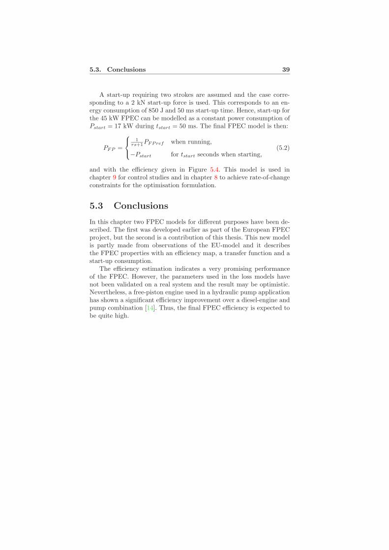
5.3. Conclusions 39
A start-up requiring two strokes are assumed and the case corre-sponding to a 2 kN start-up force is used. This corresponds to an en-ergy consumption of 850 J and 50 ms start-up time. Hence, start-up forthe 45 kW FPEC can be modelled as a constant power consumption ofPstart = 17 kW during tstart = 50 ms. The final FPEC model is then:
PFP =
1τs+1PFPref when running,
−Pstart for tstart seconds when starting,(5.2)
and with the efficiency given in Figure 5.4. This model is used inchapter 9 for control studies and in chapter 8 to achieve rate-of-changeconstraints for the optimisation formulation.
5.3 Conclusions
In this chapter two FPEC models for different purposes have been de-scribed. The first was developed earlier as part of the European FPECproject, but the second is a contribution of this thesis. This new modelis partly made from observations of the EU-model and it describesthe FPEC properties with an efficiency map, a transfer function and astart-up consumption.
The efficiency estimation indicates a very promising performanceof the FPEC. However, the parameters used in the loss models havenot been validated on a real system and the result may be optimistic.Nevertheless, a free-piston engine used in a hydraulic pump applicationhas shown a significant efficiency improvement over a diesel-engine andpump combination [14]. Thus, the final FPEC efficiency is expected tobe quite high.

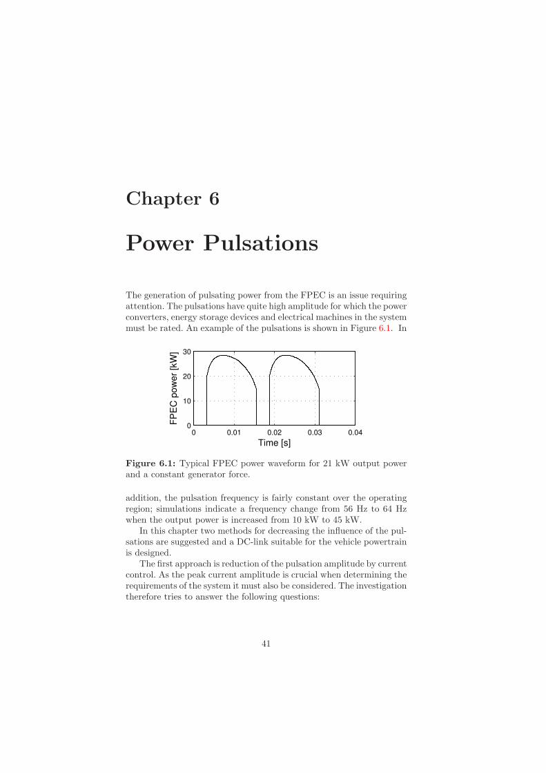
Chapter 6
Power Pulsations
The generation of pulsating power from the FPEC is an issue requiringattention. The pulsations have quite high amplitude for which the powerconverters, energy storage devices and electrical machines in the systemmust be rated. An example of the pulsations is shown in Figure 6.1. In
0 0.01 0.02 0.03 0.040
10
20
30
FP
EC
pow
er
[kW
]
Time [s]
Figure 6.1: Typical FPEC power waveform for 21 kW output powerand a constant generator force.
addition, the pulsation frequency is fairly constant over the operatingregion; simulations indicate a frequency change from 56 Hz to 64 Hzwhen the output power is increased from 10 kW to 45 kW.
In this chapter two methods for decreasing the influence of the pul-sations are suggested and a DC-link suitable for the vehicle powertrainis designed.
The first approach is reduction of the pulsation amplitude by currentcontrol. As the peak current amplitude is crucial when determining therequirements of the system it must also be considered. The investigationtherefore tries to answer the following questions:
41

42 Chapter 6. Power Pulsations
• Can the power pulsations be lowered by proper force control?
• How do the electric forces affect the current demand from thesupply system?
• Is the translator motion more affected by certain force profiles?
The second approach is based on the use of two FPEC units oper-ating with a phase shift. The phase shift makes it possible to increasethe ripple frequency and thus reduce the internal losses in the DC-linkcapacitor. Thus, a smaller and cheaper capacitor can be utilised, or thecooling requirements for a larger capacitor can be reduced. If a largecapacitor still is used its lifetime can be increased.
6.1 Reduction by Force Control
The instantaneous power is determined by the induced voltage andthe current, hence the translator velocity and the generator force. Thetranslator velocity is almost totally determined by the combustion pro-cess and the translator dynamics. The shape of the velocity profile isconsequently hard to influence. A typical waveform obtained from sim-ulation can be seen in Figure 6.2.
0 0.005 0.01 0.015 0.02 0.025 0.03
−10
−5
0
5
10
Tra
nsla
tor
velo
city [m
/s]
Time [s]
Figure 6.2: Translator velocity trajectory.
The current, on the other hand, is controllable. This gives the possi-bility to utilise it for tasks such as lowering power pulsations, increasingefficiency, reducing component demands or increase the time for faulthandling.
In the FPEC prototype it is the kinetic energy controller, describedin section 2.3, that decides the generator current. At present time itsonly task is to stabilise combustion, but if trajectory shaping is desiredit may to some extent be implemented in such a controller.

6.1. Reduction by Force Control 43
The electrical energy is produced by the electrical force doing workon the translator, transforming part of the translator’s kinetic energyto electrical. However, as mechanical energy W is an integral functionof force and position
W =
∫
F (x)dx, (6.1)
where x is translator position and F (x) is the generator force as afunction of position, the same work can be done with a number of forceprofiles F (x). Thus, in addition to combustion control some of the taskssuggested above can also be fulfilled.
Six profiles are investigated in this study, each for a specific reasonas described below.
−0.05 0 0.050
2
4
Forc
e [kN
]
Position [m]
Figure 6.3: Profile 1.
−0.05 0 0.050
2
4
Forc
e [kN
]
Position [m]
Figure 6.4: Profile 2.
Profile 1
Controlling the force to be constant over the stroke, as shown in Figure6.3, results in a square profile. Thus, it demands the lowest peak current.This profile is used for reference in the following analysis.
Profile 2
A square shaped power profile gives the highest average output powerfor a given power peak amplitude. Thus, it results in the lowest pulsa-tion amplitude. The generator force profile in Figure 6.4 is similar tothe inverse of the velocity profile so the product of force and velocityresults in a square power profile.

44 Chapter 6. Power Pulsations
Profile 3 and 4
Force profiles similar to the translator velocity give high efficiency [39].The two profiles in Figure 6.5 and Figure 6.6 are similar in shape tothe translator velocity, shown in Figure 6.2, and therefore investigated.
−0.05 0 0.050
2
4
Forc
e [
kN
]
Position [m]
Figure 6.5: Profile 3.
−0.05 0 0.050
2
4
Forc
e [
kN
]Position [m]
Figure 6.6: Profile 4.
Profile 5 and 6
To study if the translator motion is influenced more if loaded moreheavily during the initial or late part of the motion, the triangularprofiles shown in Figure 6.7 and Figure 6.8 are included in the analysis.They reduce 75% of the total load energy during the first respectivelysecond half of the stroke.
−0.05 0 0.050
2
4
Forc
e [kN
]
Position [m]
Figure 6.7: Profile 5.
−0.05 0 0.050
2
4
Forc
e [kN
]
Position [m]
Figure 6.8: Profile 6.
The profiles are implemented in the model described in section 5.1.The force controller, described in the same section, is modified so itdecides the required amplitude of the above force profiles. The profileitself is implemented as a predetermined function of position x. Thecontroller is still able to control the power output and ignition timing.

6.1. Reduction by Force Control 45
6.1.1 Conclusions
The resulting values of peak power, peak current and work are nor-malised with the values from the square profile and presented in Figure 6.9and the absolute values are provided in Table 6.1.
1 2 3 4 5 60
0.5
1
1.5
2
| Peak Power | Peak current | Work |
Norm
aliz
ed v
alu
e
Figure 6.9: Normalised values of peak power (black), peak currentdemand (medium gray) and work (white) for the investigated profiles.
Table 6.1: Results from simulation of force profiles
1 2 3 4 5 6
Ppeak [kW] 28.5 25.5 43.6 44.4 46.8 39.0Fpeak [kN] 2.9 5.0 4.3 4.5 5.9 5.4vpeak [m/s] 10.6 10.6 10.9 10.9 9.9 11.2fpower [Hz] 65 65 64 64 61 67Work [J] 329 328 330 330 339 312
−0.06 −0.04 −0.02 0 0.02 0.04 0.06
−10
−5
0
5
10
Postion [m]
Velo
city [m
/s]
Left triangle
Right triangle
Other
Figure 6.10: Velocity-position trajectories for the investigated profiles.
As seen in Figure 6.9 the inverse velocity profile results in the lowestpower pulsations, as expected. However, it also results in the third high-

46 Chapter 6. Power Pulsations
est current demand. Consequently, the price for lowering the pulsationsis a large current requirement.
Furthermore, by analysing the velocity-position waveforms in Figure6.10 it can be concluded that the translator motion is very similar forall cases except for the two triangular profiles. Hence, concentratingthe energy reduction to part of translator’s path seems to affect thetranslator motion more. This is consistent with the result in [16] wherea profile with a high force amplitude focused in the middle of translatormotion shows most influence.
6.2 Reduction by Phase Shifted Operation
When one FPEC unit is operating, the power pulsates between zeroand a peak power amplitude that is depending on the duty-cycle D.The duty-cycle is the part of the period when power is generated. Onealternative is to generate the same average power using two units, eachwith half the peak power rating and operated with 90 degrees1 phaseshift relative the other. The pulsations would then vary between thepeak power of one unit P and the peak power of two units, as seen inFigure 6.11. This reduces the ripple amplitude and increases the ripplefrequency as will be shown later.
PP
time
DT
T(a) Power ripple from one FPEC.
P
P
2P
time
DT
T(b) Power ripple from two FPECswith 90 degrees phase shift.
Figure 6.11: Power ripple, D is duty-cycle, T is pulsation period, Pis peak power and P is average output power.
However, even though this is beneficial from an electrical point ofview it may be bad from a mechanical point of view, as the mechanicalvibrations cannot be eliminated as described in section 2.3.
1Here 180 degrees corresponds to a half translator cycle, that is, start in themiddle, move to one side and back to the middle.

6.2. Reduction by Phase Shifted Operation 47
6.2.1 The DC-link Capacitor
In the middle of most electrical drive systems a DC-link capacitor issituated. This capacitor’s task is to smoothen out voltage variations andto provide short-term current capability from the primary or secondaryside of the system. It is not used for medium or long power demands,for that a super capacitor or a battery pack is more suitable. For thevoltage and energy requirements in the vehicle powertrain under studyhere, the electrolytic capacitor is commonly used.
A capacitor is very sensitive to heat, both ambient heat and heatgenerated inside, and its lifetime is determined by the internal temper-ature over time [24]. The heat inside is mainly generated by the ripplecurrent flowing through the capacitor and the model commonly usedis therefore an equivalent series resistance (ESR) in series with a ca-pacitor, as illustrated in Figure 6.12. The ESR includes, for example,
+
ESR C
Figure 6.12: Equivalent circuit of a capacitor.
resistance between the internal winding and the outer electrodes. Theinternal heat generation can then be estimated by the heat generatedin the ESR when a ripple current is flowing through it.
In Figure 6.13 the ESR as a function of the ripple current’s frequencyand the highest internal temperature, that is, the hot-spot temperature,is shown. As seen the ESR is lower for harmonics with higher frequency,hence, the capacitor losses and internal heat generation are lower for ahigh frequency ripple.
0.05 0.2
0.4 0.6
1 5
20 100 0
2040
6085
0
50
Frequency [kHz]Hot spot temp. [ °C]
ES
R [m
Ω]
Figure 6.13: Equivalent series resistance as a function of hot-spottemperature and ripple current frequency [22].

48 Chapter 6. Power Pulsations
An estimation of the FPEC ripple can be made by approximatingthe ripple curves in Figure 6.11 with Fourier series expansions. Theharmonics can then be expressed as functions of average power outputP and duty-cycle D,
p1FP(t) = P +
∞∑
n=1
2P
Dnπsin(nDπ) cos(2πfnt), (6.2)
p2FP(t) = P +
∞∑
n=1
P
Dnπsin(2πn(D − 1/2)) cos(2π2fnt). (6.3)
From (6.2) and (6.3) it can be concluded that using two units decreasesthe amplitude of the ripple power by 50% and doubles the fundamen-tal frequency. This frequency may in fact be even higher when usingtwo units, as a smaller FPEC unit probably has a higher operatingfrequency.
6.2.2 Finding a Suitable DC-link
To model the vehicle’s powertrain in chapter 7 the DC-link capacitormust be considered. However, to determine a suitable size a specificationof the DC-link demands is necessary. The following requirements weretherefore put on the capacitor bank:
1. A nominal DC-link voltage of 350 V.
2. Take one whole maximal FPEC power pulse without increasingthe voltage level from 350 V to more than 450 V.
3. Thermally handle the low frequency power ripple (60-65 Hz) fromthe FPEC.
4. Thermally handle the high frequency current ripple (10-20 kHz)from the power converter. This current is assumed to have a peakamplitude of 10% of the maximal average current.
The second dimensioning criteria will in fact decide the requiredcapacitance. By using the average current I, the power frequency f ,the maximal allowed voltage Umax and the nominal voltage U0 therequired capacitor size can be calculated as
C =I
f · (Umax − U0). (6.4)
For the numerical values given in Table 6.2 a bank with the capac-itance C ≈ 19.8 mF is required. Such a bank can be constructed by,for example, six parallel units of the EVOX-RIFA PEH169 electrolyticcapacitor. The specification for that capacitor is provided in Table 6.3.

6.2. Reduction by Phase Shifted Operation 49
Table 6.2: Specifications.
Parameter ValueNominal DC-link voltage U0 350 VMax. DC-link voltage Umax 450 VMax. average power P 45 kWMax. average current I = P /U0 130 ADuty cycle D 4/5Ripple frequency f 65 Hz
Table 6.3: Data for EVOX-RIFA PEH169 electrolytic capacitor [23].
Parameter ValueCapacitance C 3.3 mF ±20 %Rated voltage 450 VMax. hot-spot temp. 85 CRipple current at 10 kHz and 50 25 AMax. ESR at 20 and 100 Hz 34 mΩTyp. ESR at 20 and 100 Hz 15 mΩThermal resistance at 0.5 m/s 3.4 C/W
6.2.3 Conclusions
The losses in each branch, when considering the first 20 current harmon-ics IRMSnr, can be calculated by using the ESR values correspondingto each frequency ESRnr as,
Ppulse = ESR1 · IRMS1 +ESR2 · I2RMS2 + . . .+ESR20 · I
2RMS20. (6.5)
However, the losses from the ripple current produced by the power con-verter must also be considered as they will contribute to heat genera-tion. For the calculation the power converter is assumed to be switchingwith a frequency of 10 kHz and the ripple current is assumed to havean amplitude of 10 % of the load current. The converter ripple loss isthen
Pswitch = 0.1 · I2ESR10kHz. (6.6)
The losses is now calculated using ESR values interpolated from [22]and current RMS values derived from (6.2) and (6.3). The total ripplelosses Ppulse + Pswitch for each capacitor and the entire capacitor bankare given in Table 6.4.
As seen, by operating two FPECs with a phase delay the internalcapacitor losses are reduced by 70 %. This increases the lifetime of thecapacitor. However, this may not be a critical factor as the expectedlifetime of the PEH169 already is 58000 hours with a hot-spot tem-

50 Chapter 6. Power Pulsations
Table 6.4: DC-link capacitors ripple loss.
One FPEC Two FPECsSingle cap. loss 2.8 W 0.86 WCap. bank loss 17 W 5 W
perature of 85 C. In addition, the heat loss are almost negligible incomparison with a power flow through the DC-link of up to 45 kW.
Furthermore, it can be concluded that the allowed voltage levels,and not the ripple heat loss, is determining the required capacitor banksize despite the severe pulsations.

Chapter 7
Modelling of Vehicle
Components
For control and efficiency investigations a model of a vehicle powertrainis required. Vehicle simulation models are usually constructed using oneof two dominating approaches: backwards facing or forward facing. Acombination of these two can also be found in software such as Advisor[5]. A good review of available simulation packages and their differencesand application areas is given in [26].
In a backward facing model, a velocity profile is the input and it istransformed into the required power to move the vehicle. This powerdemand is propagated through the powertrain components resulting ina fuel and energy consumption. In other words, the required power iscalculated backwards from the speed profile. The drivetrain componentsare usually modelled as efficiency maps or static relationships resultingin fast simulations. The backward model is suitable for estimation offuel consumption and control strategies. The Quasi-Stationary Tool-box [7] is an example of a free Matlab/Simulink library utilising thebackwards approach.
In a forward simulation model the components are usually mod-elled using differential equations. The velocity profile is input to adriver model generating a torque and speed demand that is propagatedthrough the model. The physical flow is more like a real system andthe forward model is suitable for studies of dynamic phenomena in thepowertrain and control algorithms that should work on a real physicalplant. However, the simulation time is usually longer as the models aremore detailed and the differential equations must be solved.
For the analysis a backward facing model is utilised as fuel consump-tion of high-level control are of prime interest. The vehicle requirementsand the powertrain components and their mathematical representation
51

52 Chapter 7. Modelling of Vehicle Components
are described in this chapter. Even though modelling libraries, such asQSS or Advisor, are available most vehicle components used are mod-elled as part of this work so their behaviour can be fully understood.
Two versions of the vehicle model are developed: one model suitablefor the power management investigation in chapter 9 and the othersuitable for the linear optimisation in chapter 8.
7.1 Vehicle Parameters
A vehicle with parameters and performance corresponding to the Toy-ota Prius generation 2 is studied in this thesis. It was chosen for investi-gation for two reasons. Toyota Prius is the most successful commercialhybrid so far. This indicates that its performance is satisfactory for alarge number of customers. In addition, Toyota has been quite openabout the design and data about most drivetrain components can befound. The parameters are given in Table 7.1. From these parameters
Table 7.1: Toyota Prius vehicle specification [4].
Parameter ValueWeight, mv: 1500 kgFrontal area, Af : 1.490 × 1.725 mCoeff. of drag, Cd: 0.26Coeff. of rolling resistance, Cr: 0.01Wheel radius, rwheel : 0.3 m
the required power, torque and angular velocities for vehicle propulsioncan be calculated using the standard equations for vehicle longitudinaldynamics, given in Appendix B.
Table 7.2: Required electrical machine power, torque and speed.
Requirement Power Torque@SpeedMax. velocity 170 km/h 50 kW 70 Nm@6828 rpmAcc. 0-100 km/h at 10.9 s 121 kW 288 Nm@4010 rpmFTP75 max. torque 122 Nm@2406 rpmFTP75 max. power 37 kW 94 Nm@3770 rpm
The system must fulfil the Prius acceleration and top speed specifi-cation, thus the components must be able to deliver the required powerand torque. Furthermore, it must be able to follow a drive cycle. Thecycle used in the analysis is the FTP 75 and it is described in section7.4. To find the requirements on the electrical machine, part of themodel, that is, the longitudinal dynamics and the gearbox, is simulated

7.2. Powertrain Components 53
as explained in section 7.4. The resulting propulsion requirements aregiven in Table 7.2. As seen, the acceleration is requiring most powerfrom the system whereas the cycle demands are fairly low.
7.2 Powertrain Components
For the investigations a simulation model of a typical series drive sys-tem shown in Figure 7.1 is developed. A DC-link capacitor is used to
Electric Motor/Generator
DC-link
DC/AC
DC/DC
Battery
Electric Power
Mechanical Power
GearboxAC/DC
FPEC
Fin
al
driv
e
Brake chopper
Figure 7.1: Vehicle powertrain.
smoothen the voltage on the DC-bus. A nominal DC-link voltage of350 V is assumed. The FPEC is connected to the DC-bus via a rectifierand the battery is linked to the bus through a voltage converter. Inaddition, a brake chopper is used to prevent too high voltage levels onthe DC-link capacitor. Such levels can for example occur when energyis regenerated.
The traction electrical machine is supplied from the DC-link andcontrolled by a switch-mode inverter. It is connected to the wheels bya gearbox and a final drive.
7.2.1 Traction Electrical Machine
As the Prius has a power split hybrid topology the electrical machineand the ICE can propel the vehicle simultaneously or by themselves.Thus, neither of them has to be rated for the peak power demand asthey complement each other. The ratings for the Prius engines are givenin Table 7.3.
In an SHEV, on the other hand, the propelling electrical machinemust deliver all the traction power. But an electrical machine can beoverloaded with up to 250 % [44] for 10–30 s, which relaxes the contin-uous peak power rating of the machine. The electrical machine used insimulations is assumed to have the ratings shown in Table 7.3.

54 Chapter 7. Modelling of Vehicle Components
Table 7.3: Engine power and torque in the Toyota Prius [4] and as-sumed values for the vehicle model.
Engine Type Power@speed Torque@speedPriusGasoline (max.) 57 kW @ 5000 rpm 111 Nm @ 4200 rpmElectrical (max.) 50 kW @ 1200-1540 rpm 400 Nm @ 0-1200 rpmNet power (max.) 82 kWSHEVContinuous 42 kW @ 150–600 rad/s 280 Nm @ 0–150 rad/sOverload (250%) 105 kW @ 150–600 rad/s 700 Nm @ 0–150 rad/s
Electrical Machine Model
In the Prius a synchronous permanent magnet machine is used for elec-tric propulsion. The machine used in the model is assumed to be of thesame type. It is modelled using an efficiency map, shown in Figure 7.2,taken from the quasi-stationary toolbox [7].
ωEM
[rad/s]
TE
M [N
m]
0.8
0.85
0.9
1.15
1.2
1.3
0 100 200 300 400 500 600
−250
−200
−150
−100
−50
0
50
100
150
200
250
Figure 7.2: Efficiency map for propelling electrical machine. The thickline is enclosing the region where the machine is rated for continuousoperation.

7.2. Powertrain Components 55
7.2.2 Gearbox
The Toyota Prius has a continuously variable transmission (CVT), atransmission without fixed gear ratio. A CVT has slightly lower effi-ciency than a manual gearbox. However, the advantage is that it canconvert the incoming torque and speed to any torque-speed combina-tion resulting in the same power, as illustrated in Figure 7.3.
0 100 200 300 4000
100
200
300
ω [rad/s]
Torq
ue [
Nm
]
1 kW
5 kW
10 kW
Figure 7.3: Possible torque-speed combinations for fixed input power.
This is a desirable feature when a combustion engine is coupled tothe drive shaft using the CVT, as the engine then can be operated insuch a way that a high efficiency is obtained.
In an SHEV this is not required as the combustion engine already isdecoupled from the drive shaft. Moreover, an electrical machine is op-erating efficiently on fewer gears than a conventional engine. Therefore,a transmission with the fixed gear rations is used in this drivetrain.
Table 7.4: Gear ratios
Gear Gear ratioFirst gear, n(1) 6.5Second gear, n(2) 5.9Third gear, n(3) 4.1Fourth gear, n(4) 3.7Final gear, nfg 1.23
The gear ratios in Table 7.4 were chosen by running an optimisationprocedure on a vehicle model as suggested in [28]. This procedure findsthe gear ratios that minimises fuel consumption for the given model anddrive cycle. As the optimisation utilises a nonlinear simulation modelit cannot guarantee a global optimum. However, a local optimum issatisfactory as the procedure only is utilised to find reasonable valuesfor gear ratios.

56 Chapter 7. Modelling of Vehicle Components
Five gears are available when optimising but the result suggestsalmost the same ratio for two of the gears. This indicates that fourgears are sufficient for efficient utilisation of the electrical machine inthis powertrain.
Gearbox model
The gearbox is modelled as a torque and angular velocity conversionand a block diagram is shown in Figure 7.4. As a backwards model
Gearbox
Twheel
ωwheel
TEM
ωEM
Pwheel PEM
Figure 7.4: Gearbox model.
is used the EM torque TEM is calculated from the torque required forpropulsion Twheel using the gear ratio n(i), the final gear ratio nfg, andthe gearbox efficiency ηgear. The angular velocity is transformed in theinverse way. The expressions for the conversion are
TEM =Twheel
ηgearn(i)nfg, (7.1)
ωEM = ωwheeln(i)nfg. (7.2)
By combining (7.1) and (7.2) the relation for the powerflow on eachside of the gearbox can be expressed as
PEM = Pwheel/ηgear. (7.3)
A constant gearbox efficiency of ηgear = 95 % is assumed.
7.2.3 Battery
In the Prius system a 1.3 kWh Ni-MH battery pack is utilised. How-ever, future battery systems will be made of Lithium-Ion (Li-Ion) bat-teries. In fact, Toyota has announced that the third generation Priuswill use this technology. Li-Ion batteries have high efficiency, high en-ergy density and high power density, thus very promising properties.The battery investigated here is therefore a Li-Ion battery system.
A hybrid vehicle’s battery pack is expensive so it is desirable tominimise the aging processes to achieve a long battery lifetime.

7.2. Powertrain Components 57
The main factors that influence the aging of a Li-Ion battery are1:
• How large load that is applied.
• How long time the load is applied.
• How deep the battery is discharged during the load.
To summarise, it is not desirable to let the battery supply a large cur-rent for a long time.
The battery capacity c describes the total number of Ampere-hoursthat can be withdrawn from battery under specified conditions of dis-charge [37]. The load rate are described as parts of c [37], hence theload rate c/2 for a battery with 2 Ah capacity corresponds to 1 A loadcurrent.
Furthermore, when the same load energy is applied to a batteryhaving a large capacity, compared to one with smaller capacity, thelarger battery has shallower depth of discharge. Thus, the battery ca-pacity must be carefully chosen to achieve a reasonable lifetime underthe expected load.
Parameters for the battery system used in the model are taken from[41] where a Li-Ion battery pack is compared to the Prius Ni-MH bat-tery. This battery pack is constructed using ICR18650 Li-Ion cylindricalcells with the specification given in Table 7.5.
Battery model
The detail level of battery models in the literature varies from verydetailed models describing internal chemical reactions to simpler modelssuch as the Thevenin equivalent. As the battery efficiency is of greatimportance for the system efficiency, it must be modelled carefully. Therequired characteristics for a realistic model suitable for simulations are:
• The losses should depend on the battery load.
• The losses should depend on the present energy content.
A battery cell model with the above mentioned behaviour is a resistancein series with a state-of-charge dependent voltage source as illustratedin Figure 7.5. The battery model is described by the following mathe-matical expressions. The state-of-charge SoC is the integral of the netpowerflow into the battery, hence the power at the battery terminalsPbatt minus the loss Ploss,
SoC(t) = SoC(tstart) +1
Wbatt
∫ t
tstart
Pbatt(τ) − Ploss(τ) dτ. (7.4)
1Concluded after discussion with Dr. Marten Behm at the division of AppliedChemistry, KTH.

58 Chapter 7. Modelling of Vehicle Components
E
+
-
+
e(SoC)
R
Pbatt
Figure 7.5: Nonlinear battery model used in simulation.
The loss Ploss is the loss in the resistor R
Ploss(t) = Ri(t)2. (7.5)
The current i(t) is a nonlinear function of the internal voltage e(SoC),the resistance R and the power flow Pbatt
i(t) = −e(SoC)
2R+
√(
e(SoC)
2R
)2
+Pbatt
R. (7.6)
where the internal voltage e(SoC) has the following dependence ofstate-of-charge
e(SoC) = E0 − k(0.6 − SoC). (7.7)
The parameters used for the model are given in Table 7.5.A Li-Ion based battery pack with higher energy capacity and lower
weight than the battery pack in the Prius is suggested in [41]. Datacorresponding to that pack is used for modelling here. The value onthe internal resistance R is chosen so that the battery fulfils the powerrequirement and has a realistic efficiency.
The battery pack is assumed to consist of 100 series connected mod-ules. This results in the battery pack performance given in Table 7.5.
Table 7.5: Battery cell model parameters.
Model Parameter ValueOpen circuit voltage E0 3.95 Vk 0.625 V/SoCBattery pack data ValueNr. of modules in series, cellnr 100Nominal voltage (SoC = 0.5) 380 VEnergy capacity 2072 WhInternal resistance R 1.65 Ω

7.2. Powertrain Components 59
−20 0 200.4
0.6
0.8
1
0.20.40.60.81.0
Load power [kW]
Eff
icie
ncy
Figure 7.6: Instantaneouscharge and discharge efficiencyas function of load power andstate-of-charge.
0 5 10 15 200
0.5
1
Constant load power [kW]
Cycle
eff
icie
ncy
Figure 7.7: Cycle efficiency forconstant loads.
To validate the model’s behaviour two measures of battery efficiencyare studied. First, the instantaneous charge and discharge efficiency,where the discharge efficiency is the power at the terminals Pbatt overthe power delivered from the battery inside
ηdis =Pbatt
Pbatt + Ploss. (7.8)
The charge efficiency is the power that actually charges the batteryover the power entering the battery
ηch =Pbatt − Ploss
Pbatt. (7.9)
In Figure 7.6 efficiency curves for different state-of-charge values aredisplayed. As seen, the charge and discharge efficiency is dependent onboth the state-of-charge and the load. Furthermore, the efficiency de-creases with higher charge and discharge power, which is reasonable asloading a battery hard generates more losses. In addition, the efficiencydecreases for lower state-of-charge values. When charging, here repre-sented by positive power, the efficiency is slightly higher for a higherstate-of-charge. This is consistent with the behaviour of a Li-Ion battery[35].
The second efficiency measure analysed is the Joule efficiency or thecycle efficiency. It is the ratio of discharge energy over charge energy,required to reach the initial state-of-charge, when the battery is fullycycled. For a new Lithium-Ion battery cell this efficiency is roughly94 % when loaded with c/5 whereas a Lead-acid battery has a peakefficiency of 80 % [35].
The Joule efficiency for this model is displayed in Figure 7.7. Thecurve is achieved by totally discharging the battery using a constant

60 Chapter 7. Modelling of Vehicle Components
power and then recharging it using the same constant power level. Asseen, the cycle efficiency decreases during heavy load and for low loadsthe battery has an efficiency above 90 %, which is consistent with thevalues in [35].
The above observations indicate that this fairly simple battery modelhas the desired properties and behaves in a realistic way.
7.2.4 Power Electronics
Power electronics are essential for the hybrid electric system. It is usedfor control of the electrical machines and conversion between differentvoltage levels in the system.
As discussed earlier several power electronic devices are used in thispowertrain. The efficiency of these devices depends on the voltage andcurrent but the average efficiency is usually high. In addition, a powerelectronic device is fast compared to the other powertrain components.The devices are therefore simply modelled as a constant scaling ηconv
of the power input
Pinηconv = Pout. (7.10)
An efficiency of ηconv = 97 % is assumed for all power electronics inthis vehicle.
7.2.5 DC-link
The DC-link capacitor was discussed and dimensioned in chapter 6. Itis modelled as storage of the FPEC power flow PFP , the battery powerflow Pbatt and the load disturbance Pload, over the present DC-linkvoltage UDC
UDC(t) = UDC(tstart)+1
C
∫ t
tstart
(PFP (τ)+Pbatt(τ)−Pload(τ)
)/UDC(τ)dτ.
(7.11)
The power dissipated in the brake chopper is modelled as a sat-uration of the capacitor’s voltage level. Hence, when the capacitor issaturated any additional power entering the DC-link is dissipated.
As the load disturbance is acting directly on the DC-link the ca-pacitor’s voltage level must be controlled to assure that it is withinthe allowed limit. Furthermore, the capacitor cannot provide power forlong time intervals so it requires a controller to not be totally drainedfrom time to time. The DC-link voltage is preferably kept around itsnominal level of 350 V but variations are allowed and small variationshave minor effect on the system.

7.2. Powertrain Components 61
Recently, a nonlinear control law for buffer control has been sug-gested [47, 49]. The nonlinear law F (UDC) is the tangent function
F (UDC) = K · tan((UDC − a)/b
)(7.12)
where, UDC is the present DC-link voltage and a, b, and K are tuningparameters. This nonlinear controller gives a small control output forsmall variations around the nominal voltage value and a very largeoutput when the voltage is reaching the limits, as seen in Figure 7.8.This is a desirable behaviour that cannot be achieved using the morecommon proportional controller. The output of the DC-link controller
200 250 300 350 400 450 500
−50
0
50
DC−link voltage [V]
Contr
ol outp
ut
[kW
]
Figure 7.8: Controller output as function of DC-link voltage. Thecontroller parameters are a = 350, b = 400 and K = 13000.
is added to the power management controller’s load demand input.Power management is discussed more in chapter 9.
7.2.6 Auxiliary Load
The auxiliary loads, for example fuel pump and internal heating, aremodelled as a constant power consumption of 600 W. This is typicalaverage load power for a vehicle’s electrical system [2].
7.2.7 Diesel Generator
For comparison an SHEV equipped with a diesel generator is chosenas reference vehicle. In the reference vehicle the FPEC is replaced bya conventional diesel generator while the other powertrain componentsare the same. A diesel generator is a combination of an ICE and anelectrical generator. The generator can provide 45 kW power and theresulting efficiency is obtained by combining the two efficiency mapsfrom [6] shown in Figure 7.9 and Figure 7.10.
In an SHEV any torque-speed combination providing the requiredpower can be chosen, as the diesel-generator does not have a mechanical

62 Chapter 7. Modelling of Vehicle Components
0.2
0.25
0.3 0.350.4
Speed [rad/s]
Torq
ue [N
m]
0 100 200 300 4000
20
40
60
80
100
Figure 7.9: Diesel combustionengine efficiency map.
0.5
0.6
0.7
0.8
0.9
Speed [rad/s]
Torq
ue [
Nm
]
0 100 200 300 4000
50
100
Figure 7.10: Electrical genera-tor efficiency map.
connection to the drive shaft. However, the torque-speed combinationwith the highest efficiency for the given power is preferably chosen. Theoptimal points for the torque-speed map are displayed in Figure 7.11and the resulting efficiency as function of power is presented in Figure7.12.
0.25
0.35
Speed [rad/s]
0.2
Torq
ue [N
m]
0 100 200 300 4000
50
100
Figure 7.11: Diesel generatorefficiency map and optimal op-erating points.
0 10 20 30 400
0.1
0.2
0.3
0.4
Diesel generator power [kW]
Optim
al effic
iency
Figure 7.12: Optimal dieselgenerator efficiency as functionof power.
7.3 Modelling for Optimisation
For the optimisation procedure, that will be described in chapter 8, amodel simpler than the one described earlier is sufficient. As the powermanagement primary affects the DC-link capacitor, the battery andFPEC, these parts are most important to include in the optimisationformulation. The required power is precalculated by simulating part of

7.3. Modelling for Optimisation 63
the drivetrain as shown in Figure 7.13.
DC-link
Battery
Brakechopper
EM efficiencymap
Gear-boxVehicle
dynamics
Precalculation
Pload
ηdis ηchPchPdis
Poverload
PFP
ηFP
Figure 7.13: Structure of state-space optimisation model.
7.3.1 State-space Model
The system is modelled as two power buffers: the DC-link capacitor andthe battery. The battery is modelled with state-of-charge as the out-put. The powerflow in and out from the battery terminals is separatedinto two positive power flows, Pch and Pdis. This makes it possible tohave different values for the battery charge efficiency ηch and dischargeefficiency ηdis. The battery state-of-charge is described as the integralof the net powerflow into the battery
SoC(t) = SoC(tstart)+1
Wbatt
∫ t
tstart
ηchPch(τ)−ηdisPdis(τ) dτ. (7.13)
The capacitor can be charged using FPEC power PFP or the bat-tery power. The load power Pload is considered to be a disturbanceacting directly on the DC-link. Furthermore, it is possible to dischargeexcess power in the brake chopper Pbr. The present energy level of thecapacitor can be expressed as
Wcond(t) = Wcond(tstart)+
∫ t
tstart
PFP (τ)+Pdis(τ)−Pch(τ)−Pbr(τ)−Pload(τ) dτ.
(7.14)Equation (7.13)-(7.14) can be expressed as a continuous state-spacemodel
x(t) = Bu(t) + Fv(t), (7.15)
by choosing the state vector x(t) as
x(t) =
[SoC(t)
Wcond(t)
]
, (7.16)

64 Chapter 7. Modelling of Vehicle Components
the input vector u(t) as
u(t) =
PFP (t)Pch(t)Pdis(t)Pbr(t)
, (7.17)
and the disturbance v(t) as
v(t) = Pload(t). (7.18)
The matrices are
B =
[0 ηch/Wbatt −ηdis/Wbatt 01 −1 1 −1
]
, F =
[0−1
]
. (7.19)
As there is no dependence on x(t) in (7.15) and thus no dynamics thismodel simply represents two buffers that can be filled and drained usingthe control input vector u(t).
7.3.2 Discretisation
To be able to use this system description in a linear program it mustbe discretised. Several methods to convert continuous time models todiscrete time are available but here the zero-order hold approach [42]is chosen. This method can be seen as sampling the continuous systemwith the control signal kept constant during the sampling interval. Theresult is a discrete description of the system
x[k + 1] = Adx[k] + Bdu[k] + Fdv[k], (7.20)
where k is the time index. The matrices Bd and Fd differs from B andF due to the discretisation. Moreover, the discretisation introduces anadditional matrix Ad.
7.4 Drive Cycle Analysis
An initial analysis of the power and energy requirements for the systemis made by using part of the model, that is, vehicle dynamics, gearbox,and propelling electrical machine. This part of the model, shown inFigure 7.14 is creating the load disturbance acting on the DC-link andthis disturbance is the same for all investigations in this thesis. Themodel is also used to find the electrical machine requirements discussedin section 7.1. In addition, some interesting conclusions can be drawnusing this model.
The cycle that will be used in all investigations is the federal testprocedure 75 (FTP75) shown in Figure 7.15. This is a cycle used for

7.4. Drive Cycle Analysis 65
Vehicle
Dynamics
Gear-
boxEM efficiency
map
v(t)Tv(t)
ω(t)
TEM (t)
ωEM (t)
PEM (t)
Figure 7.14: Power
emission certification in the US, Sweden, Mexico, Switzerland and Aus-tralia. It is a real velocity profile measured during morning traffic inLos Angeles and as seen, it has both slow driving around 50 km/h,highway driving around 90 km/h and a number of standstills. Hence,it is representative for most driving conditions and therefore chosen forthis study.
0 500 1000 15000
20
40
60
80
100
FT
P75 d
rive c
ycle
[km
/h]
Time [s]
Figure 7.15: The federal test procedure 75 drive cycle
By analysis of the power flow shown it can be concluded that ideally26 % of the required propulsion energy can be acquired by regeneration.The power flow over time is shown in Figure 7.16. However, to utiliseall this energy the battery’s capacity must be sufficiently large.
Each time the vehicle is retarding, power is regenerated into thesystem for some time. This results in a different amount of energyregenerated each time the vehicle retards. This energy will be referredto as consecutive regenerated energy. The distribution of the consecutiveregenerated energy, for the FTP75 cycle, is shown in Figure 7.17.
As seen in Figure 7.17, the largest amount of energy continuouslyregenerated is approximately 150 kJ or 41.7 Wh, which is only 2 % ofthe total battery capacity of 2.072 kWh.
The distribution of power flowing in and out of the electrical ma-chine is shown in Figure 7.18. Most of the time the power level is be-
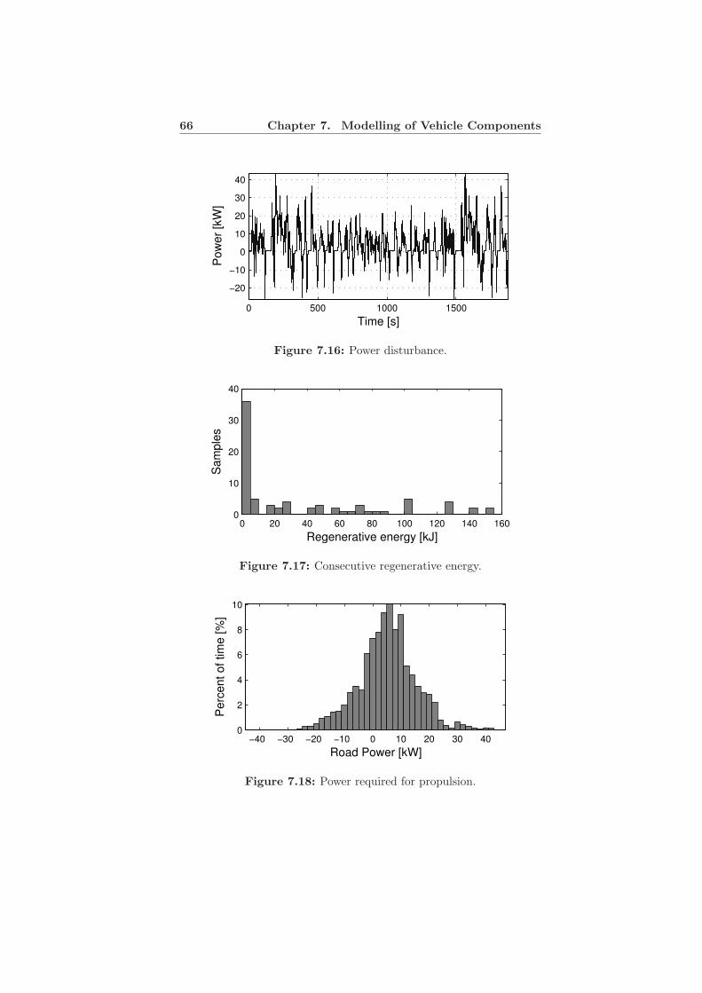
66 Chapter 7. Modelling of Vehicle Components
0 500 1000 1500
−20
−10
0
10
20
30
40
Time [s]
Pow
er
[kW
]
Figure 7.16: Power disturbance.
0 20 40 60 80 100 120 140 1600
10
20
30
40
Regenerative energy [kJ]
Sam
ple
s
Figure 7.17: Consecutive regenerative energy.
−40 −30 −20 −10 0 10 20 30 400
2
4
6
8
10
Road Power [kW]
Perc
ent of tim
e [%
]
Figure 7.18: Power required for propulsion.

7.4. Drive Cycle Analysis 67
tween -20 kW and 20 kW, hence it is desirable to have high systemefficiency for this load interval.
Finally, a benchmark value for the lowest fuel consumption for thispowertrain can be found. The FPEC model has an estimated peakefficiency of approximately 43 %. Simulating a powertrain where theFPEC provides all traction power, operating with the peak efficiencyall the time, and where all energy can be regenerated with 100 % effi-ciency results in a fuel consumption of 0.35 l/10 km. Thus, lower fuelconsumption is hard to achieve with this powertrain in the later in-vestigations, as battery losses, power converter losses and FPEC lossesthen are present. In addition, not all available regeneration energy canusually be utilised.
In the next chapter another benchmark value is found by usinglinear optimisation and the powertrain model.


Chapter 8
Finding the Optimal
Fuel Consumption
As there are several power sources in an HEV, the efficiency, and thusthe fuel consumption, is dependent on the power control strategy used.That is, a good utilisation and interaction between the power sourcesresults in a high efficiency. This dependence makes it hard to decidehow well a control strategy performs by just doing simulations of thesystem.
Optimisation is one tool that can be used to facilitate these tasks.The results from an optimisation procedure are hopefully close to thebest achievable, and can therefore be used as a benchmark to knowwhen a controller or powertrain design is good enough. Another fea-ture is that limits on the systems states can be incorporated in theevaluation.
In this chapter the ”optimal” fuel consumption for the powertraindescribed by the models developed in chapter 7 is investigated. Linearoptimisation is chosen to achieve a good compromise between solutiontime and accuracy. The state-space model developed in chapter 7 isused in the problem formulation. However, to reduce the number of ap-proximations the load disturbance is precalculated using the nonlinearsimulation model.
8.1 Linear programming
In a linear program (LP), a goal function is to be minimised or max-imised. This function is a linear combination of the optimisation vari-able vector u,
g(u) = minu
fT u, (8.1)
69

70 Chapter 8. Finding the Optimal Fuel Consumption
where f is a vector of constants. The optimisation constraints are linearequalities or inequalities of the optimisation vector u
Au ≤ b (8.2)
Cu = d, (8.3)
where b and d are vectors and A and C are matrices.One great benefit of LP is that the problem formulation is convex,
that is, only one optimal point exists. As a result, the optimal solutionfound is the global optimum. Moreover, efficient solvers are available,so problems with a large number of variables can still be solved inreasonable time.
The drawback when used for vehicle evaluation is that everythingmust be formulated as linear or piecewise linear functions. This mayrequire major approximations. In addition, the problem must be discre-tised in time, which may introduce discrepancy from the real solution.
8.1.1 Cost Function
Fuel consumption is directly related to FPEC usage. The volume fuelrate for diesel Vdiesel can be calculated from FPEC power PFP usingthe diesel density ρdiesel and the specific calorific value qHV ,
Vdiesel = PFP /(qHV · ρdiesel). (8.4)
Typical values for diesel are qHV = 42.5 MJ/l and ρdiesel = 0.83 J/kg[2]. The fuel consumption rate is estimated by using the FPEC efficiencymap from chapter 5 and expression (8.4). The fuel rate is shown inFigure 8.1 and it can be concluded that it is an almost linear functionof delivered power.
0 10 20 30 40 500
1
2
3
FPEC power [kW]
Fuel consum
ption r
ate
[ml/s]
Figure 8.1: Fuel consumption rate as function of power.
The energy consumption, on the other hand, is not linear. Figure 8.2illustrates the amount of fuel required to produce 1 kWh of electrical

8.1. Linear programming 71
energy when running the FPEC at a constant power. Thus, to achievethe lowest possible consumption the FPEC should not be operatedbelow 10 kW for longer periods.
10 20 30 400
0.2
0.4
0.6
0.8
FPEC power [kW]
Fuel consum
ption[l]
Figure 8.2: The amount of fuel required to produce 1 kWh as functionof power.
Nevertheless, this effect is ignored to achieve a fairly simple linearformulation. The cost minimised over the cycle is the total FPEC energyused
WFPEC = min ·N∑
k=0
PFP [k]. (8.5)
The fuel consumption is then calculated using FPEC power and thefuel rate map in Figure 8.1. Hence, the FPEC efficiency is consideredin the fuel consumption calculation but the optimisation procedure isnot affected by it.
8.1.2 Constraints
The constraints used in this optimisation are introduced for three rea-sons. The powertrain has physical limitations that introduce inequal-ity constraints. Charge sustaining behaviour is desired, which requiresequality constraints. Finally, the discrete state-space representation ofthe system introduces equality constraints.
Physical constraints
The components in an electrical powertrain have physical limitations.These limitations are, for example, sizes of the energy buffers or con-straints on how fast the power level can be changed. The FPEC power-train is assumed to be under the following constraints. The FPEC canonly generate power (not absorb) and has a limit on the peak power itcan generate
0 ≤ PFP ≤ Pmax. (8.6)

72 Chapter 8. Finding the Optimal Fuel Consumption
Moreover, it cannot change between power levels infinitely fast duringa sample interval, which results in a rate-of-change constraint
− PFPmax ≤ PFP ≤ PFPmax, (8.7)
which in discrete time can be formulated as
− ∆t · PFPmax ≤ |PFD[k] − PFD[k − 1]| ≤ ∆t · PFPmax, (8.8)
where k is the time index and ∆t the sample time. The battery haslimits on how much power it can provide
− Pbattmax ≤ Pdis − Pch ≤ Pbattmax, (8.9)
where Pdis − Pch is the net battery power flow at the terminals. TheDC-link capacitor has limitations on the allowed DC-link voltage
UDCmin ≤ UDC ≤ UDCmax, (8.10)
Finally, to achieve high efficiency and long lifetime of the battery itshould not be cycled too deep. Therefore it is desirable to keep the SoCwithin certain limits
SoCmin ≤ SoC ≤ SoCmax. (8.11)
Charge sustaining constraints
A charge sustaining power management strategy aims to keep thecharge of the energy storage within certain limits during driving. Thisis the desired behaviour of the FPEC vehicle and to assure charge sus-taining behaviour, the final values of the energy buffers are forced tobe same as the initial.
SoC[kstart] = SoC[kend] (8.12)
UDC [kstart] = UDC [kend] (8.13)
Without these end constraints the optimisation would favour a strategydraining the buffers as much as possible as this results in a lower FPECusage.
State-space constraints
The discrete formulation is determined by the initial value x0 = x[0],the known disturbance v[k] and the unknown control values u[k]. Toillustrate how this can be reformulated into an equality constraint, thestate-space description (7.20) is investigated over three timesteps,
x[1] = Adx0 + Bdu[0] + Fdv[0] (8.14)
x[2] = Adx[1] + Bdu[1] + Fdv[1] (8.15)
x[3] = Adx[2] + Bdu[2] + Fdv[2] (8.16)

8.2. Implementation 73
By substituting (8.14) into (8.15) and (8.15) into (8.16) and using vectornotation (8.14)-(8.16) can be expressed as
xd =
Ad
A2d
A3d
︸ ︷︷ ︸
A
x0 +
Bd 0 0AdBd Bd 0A2
dBd AdBd Bd
︸ ︷︷ ︸
B
ud +
Fd 0AdFd Fd 0A2
dFd AdFd Fd
︸ ︷︷ ︸
F
vd,
(8.17)with
xd =
x[1]x[2]x[3]
, ud =
u[0]u[1]u[2]
and vd =
v[0]v[1]v[2]
. (8.18)
Equation (8.17) can be expressed as a linear equality constraint on theLP form (8.3) by moving everything not depending on ud to the righthand side,
Bud = xd − Ax0 − F vd. (8.19)
The above procedure can be generalised for N timesteps by expandingthe matrices A, B and F . As seen, the size of these matrices and vec-tors depends on both the number of states and the number of discretetimesteps that are investigated. Hence, decreasing the sample time re-sults in more timesteps per second and larger matrices and vectors.
8.2 Implementation
Reformulating the problem and creating the matrices as described ear-lier are a quite tedious effort. An excellent modelling language thatfacilitates this in Matlab is Yalmip [40]. Yalmip also works as an in-terface to a large number of numerical solvers. The solver used in thisanalysis is SDPT3 [53], a Matlab software for semidefinite-quadratic-linear programming.
Vehicle
Dynamics
Gear-
box
EM efficiency
mapDC-link
v(t)Tv(t)
ωv(t)
Tg(t)
ωg(t)
Pdist(t)
Figure 8.3: Model for precalculation of power disturbance.
The power used to propel the vehicle is seen as a disturbance actingon the DC-link capacitor. The disturbance Pdist is originating from thedrive cycle and precalculated using a model of part of the powertrain,as shown in Figure 8.3 and discussed in section 7.4.

74 Chapter 8. Finding the Optimal Fuel Consumption
8.2.1 Optimisation Formulation
When the cost function and the constraints are determined, the finalformulation of the optimisation problem can be summarised as follows.
Optimisation Formulation
For the given powertrain under the power disturbance (7.18), keep theDC-link voltage within the given limits using the available power sourcesPFP , Pbatt and the brake chopper Pbr so that the energy consumptionis minimised
WFPEC = min
N∑
k=0
PFP [k]. (8.20)
This minimisation should be done subject to the powertrain limitations
0 ≤ PFP ≤ Pmax
−PFPmax ≤ PFP ≤ PFPmax
−Pbattmax ≤ Pdis − Pch ≤ Pbattmax
SoCmin ≤ SoC ≤ SoCmax
(8.21)
the buffer end constraints and the state-space model constraints
SoC[kstart] = SoC[kend]
UDC [kstart] = UDC [kend]
Bud = xd − Ax0 − F vd.
The numerical values used for the model and the constraints aregiven in Table 8.1.
8.2.2 Sample Time
As discussed earlier, using a small discretisation time results in largematrices and vectors. This may give numerical problems in the solveror computer memory issues. The calculation time is also increased. Onthe other hand, using a too large discretisation time may result in abad approximation of the continuous model.
To get an indication of how the discretisation time affects the fi-nal result, the optimisation is performed on the first 430 seconds ofthe FTP75 cycle using models discretised with different sample times.The times investigated are 1 s, 0.5 s, 0.25 s, 0.1 s and 0.05 s and theresult is presented in Table 8.2. The relative improvement on the lasttable row corresponds to how much lower the fuel consumption result iscompared to optimising with a model discretised with the sample timeto the left. That is, using Ts = 0.5 s gives approximately 2.1 % lower

8.2. Implementation 75
Table 8.1: Numerical values used in the optimisation formulation.
Model parameters ValueDC-link capacitor: 20 mFDiscretisation time, ∆t 0.1 sBattery energy content, Wbatt 2.072 kWhConstraintsPFPmax 45 kW
PFPmax 7.5 kW/∆tSoCmin 30 %SoCmax 70 %±Pbattmax ±24 kWUDCmax 400 VUDCmin 300 VInitial valuesSoCinit 70 %UDCinit 350 V
Table 8.2: Fuel consumption for the investigated sample times.
Parameter ValueSample time Ts 1s 0.5s 0.25s 0.1s 0.05sFuel consumption [l/10km] 0.392 0.3857 0.3814 0.3789 0.3780Relative improvement - 2.1 % 1.12 % 0.67 % 0.2 %

76 Chapter 8. Finding the Optimal Fuel Consumption
result than using Ts = 1 s. To get a reasonable compromise betweencalculation time and accuracy the discretisation time used in the fol-lowing optimisation analysis is chosen to 0.1 s. Using the even smallertimestep Ts = 0.05 s would only change the result with 0.2 % .
8.3 Results and Conclusions
First, it should be noted that this optimisation suggests control valuesfor battery and FPEC power when the entire drive cycle is known inadvance. Thus, the behaviour is non-casual and the resulting lowest fuelconsumption is hard to achieve with a real implementable controller.
The state-of-charge variation over the cycle can be seen as thethicker line in Figure 8.4. The full available range of 30–70 % SoCis far from fully utilised and the cycling is very shallow for the 2 kWhbattery. In fact, when solving with reduced battery capacity, it turnsout that the capacity can be reduced more than ten times withoutincrease of the optimal fuel consumption for the investigated cycle.
The variation when using a ten times smaller battery (0.2 kWh),is also shown in Figure 8.4. As seen, it utilises more of the availablerange but the smaller capacity results in deeper cycling. To assure areasonable battery lifetime a capacity somewhere in between the valuesinvestigated here is probably desirable.
0 500 1000 150030
40
50
60
70
Battery
SoC
[%
]
Time [s]
Figure 8.4: Battery state-of-charge variations. The thick line is for the2 kWh battery whereas the thinner line is for the 0.2 kWh battery.
The battery power flow is seen in Figure 8.5. The largest powerpeaks occur when charging, and from time to time they are close to therated battery peak power of 24 kW. Hence, an energy storage with lessenergy capacity and at least the same power capability is desirable. Asupercapacitor is a suitable alternative with these properties.

8.3. Results and Conclusions 77
0 500 1000 1500
−20
−10
0
10
20
Batt
ery
pow
er
[kW
]
Time [s]
Figure 8.5: Battery power, positive values are discharging the battery.
As seen in Figure 8.6, the FPEC is working frequently at low loadswhere the efficiency is poor. This is a result of the linear cost-function asdiscussed in section 8.2. The optimisation algorithm minimises the sumof FPEC power and does not consider the FPEC efficiency. It mightbe possible to include this into the problem formulation by having aquadratic or perhaps a nonlinear cost function. However, as the maingoal of this optimisation is to find a benchmark value for power man-agement strategies, no attempts were made to improve the formulation.
0 5 10 15 20 25 30 35 40 450
0.1
0.2
0.3
0.4
0.5
ηF
PE
C &
num
ber
of sam
ple
s
Power [kW]
Figure 8.6: Efficiency of the FPEC (cross points) and a histogramof the number of samples spent in a power interval. Operating pointsbelow 500 W are excluded.
Finally, the optimal fuel consumption for different battery efficien-cies are given in Table 8.3. For reference, a system without batteryis investigated. The optimisation finds a feasible solution for a system

78 Chapter 8. Finding the Optimal Fuel Consumption
Table 8.3: Fuel consumption results from optimisation.
Battery eff. Fuel cons. [l/10 km]No batt. 0.464
0.80 0.4000.85 0.3930.90 0.3850.95 0.3770.99 0.370
without battery. Hence, under the optimisation constraints used, theFPEC and the DC-link capacitor can handle the power disturbance bythemselves. However, as mentioned earlier this procedure is non-causalso it can compensate for the disturbances before they actually haveaffected the system. This compensation is hard to achieve, to the sameextent, in a real system. Thus, some kind of energy or power buffer isneeded. Nevertheless, the result indicates that a fairly small buffer maybe sufficient.
Using an almost ideal battery, that is, with 99 % efficiency results in0.37 l/10km. The almost ideal vehicle estimation in chapter 7 resultedin 0.35 l/10km. Hence, introducing a varying FPEC efficiency into themodel has increased the fuel consumption with 0.02 l/10 km or 5 %compared to the ideal vehicle.
In the next chapter the fuel consumption under different power man-agement strategies will be analysed. The results presented above willthen be useful when analysing how good these strategies really are.

Chapter 9
Power Management
To utilise the full potential of a hybrid vehicle it is important to use itsavailable power sources in an efficient way. As mentioned in chapter 4,common strategies for SHEVs are on-off or load-following strategies.However, controlling an FPEC using an on-off strategy would not takeadvantage of its main benefit: the rapid transient response.
In this chapter, three power management strategies are investigated.The first strategy is a load following strategy using one FPEC unit. Thesecond is a load-following strategy with two FPEC units; combiningtwo units may increase the system efficiency at low loads. Finally, astrategy, based on an equivalent consumption minimisation, is adaptedto the FPEC powertrain and analysed.
BatteryController
Measurements
Traction power demand
Traction EMController
E MFPECDC-link
BatteryController
DC-linkController
FPECcontroller
Power Management Controller
Figure 9.1: Example of controller structure.
The strategies investigated are operating on a high system level andshould only decide how the power should flow. This information is thensent to the low-level controllers in the system as seen in Figure 9.1.To make the decision, information about the system’s present states isrequired. The states can be measured or estimated but in this analysisthey are just assumed available.
79

80 Chapter 9. Power Management
The power demand is assumed to be available and is used as a feed-forward signal to the power management controller. This signal willprobably be available in a real system as the power demand mainly isdetermined by the required traction power, and the traction electricalmachine requires some kind of power control.
The control strategies investigated are all charge sustaining. There-fore, to make the simulation results regarding fuel consumption compa-rable, the battery is recharged to its initial state-of-charge value (70 %)at the end of the cycle. When recharging, the FPEC is assumed to beoperating at a power of 15 kW and thus quite high efficiency. The fuelconsumption after recharging will be referred to as corrected fuel con-sumption.
9.1 Load Following Strategies
As the FPEC has a rapid transient response and high efficiency overmajor part of its operating region it should be able to efficiently followa fluctuating power demand. In the heavy-duty truck study [36] such astrategy gave the most promising result. Two load-following strategiesfor the FPEC powertrain are therefore analysed here.
The first strategy is utilising a singular FPEC unit. The strategymakes the FPEC follow the load demand and the required additionaltransient power is provided by the battery.
510
1520
5
10
0.45
0.5
0.55
0.6
Start power [kW]Stop power [kW]
Corr
fuel [l/1
0km
]
Figure 9.2: Corrected fuel consumption as function of FPEC startand stop threshold values.
To avoid FPEC operation at low power levels, where the efficiencyalso is low, start and stop power thresholds are used. These thresholdlevels are the available tuning parameters for this strategy. To optimisethe values for this cycle the vehicle is simulated using 1–20 kN as astart threshold combined with 2–10 kN as stop values. The correctedfuel consumption for these combinations is presented in Figure 9.2.

9.1. Load Following Strategies 81
By analysis of the fuel consumption results, after iteration, a mini-mum corresponding to a start threshold of 7 kW and a stop thresholdof 1 kW is found. These levels are therefore chosen for further investi-gation. However, in the histogram of operating points, shown in Figure9.3, it can be seen that the FPEC is operating frequently at powerlevels lower than 10 kW and thus with a low efficiency.
10 20 30 400
0.1
0.2
0.3
0.4
FPEC power [kW]
Figure 9.3: FPEC operating point intensity and FPEC efficiency asfunction of power for 9 kW start threshold and 1 kW stop threshold.
One simple approach to avoid this operating region is to also set thestop threshold to 10 kW as the FPEC then would not operate at thelow power levels. However, by looking at the fuel consumption surfacein Figure 9.2 it can be concluded that using 10 kW as stop thresholdin fact increases the fuel consumption.
Another approach is to utilise two or more FPECs instead of justone. A smaller unit has higher efficiency at the lower power levels thana larger one. In addition, the number of active units can be determinedby the load. Hence, some units can be turned off when the load is low,which forces the active units to operate at higher power, thus withhigher efficiency.
10 20 30 400
0.1
0.2
0.3
0.4
Effic
iency
FPEC power [kW]
Figure 9.4: Efficiency curves for a 45 kW (dashed line) and 22.5 kW(solid line) FPEC unit.

82 Chapter 9. Power Management
The curves in Figure 9.4 illustrate the FPEC efficiencies under theassumption that downscaling the 45 kW FPEC to a 22.5 kW unit justscales the efficiency curve. As seen, the smaller unit has up to 10 %higher efficiency value at low loads. To investigate the potential effi-ciency increase of this approach a load-following strategy using twoFPEC units is studied.
Two units require four threshold levels to be tuned: the start thresh-olds for each unit as well as the stop thresholds. To find suitable valuesfor these threshold values, simulations is iterated in the same manneras for the one FPEC case and the thresholds resulting in the lowestfuel consumption is chosen. The thresholds for the two cases are givenin Table 9.1.
Table 9.1: Threshold levels for load following strategies.
Start 1 Stop 1 Start 2 Stop 2
One FPEC: 7 kW 1 kWTwo FPECs: 8 kW 1 kW 24 kW 8 kW
9.2 The Equivalent Consumption Minimi-
sation Strategy
Strategies defined by a set of rules and thresholds, as in the two load-following strategies just discussed, are probably used in most hybrid ve-hicles today. However, finding threshold levels and switching points forsuch strategies requires extensive simulations and testing on a real sys-tem to assure high efficiency. Furthermore, in a real vehicle the drivingcharacteristics and the cycle are changing over time and it is thereforehard to optimise the values for all possible driving conditions. A moresystematic way to find thresholds and control the power flow based onthe system properties and not on the drive cycle is desirable.
One method that may achieve this has been suggested in the lit-erature under the name equivalent consumption minimisation strategy(ECMS). It is based on the power flow and the efficiencies of the systemcomponents. Thus, it is a generic method that can be applied to anyhybrid powertrain.
The ECMS minimises a weighted cost of power source usage everysample time. The cost is calculated by transforming the required energyinto one common energy form: an equivalent consumption, hence thename. The combination of power sources minimising the stated cost,subject to the system constraints, is then used.
The strategy is derived under the assumption of a charge sustainingsystem. The main ideas behind the strategy are:

9.2. The Equivalent Consumption Minimisation Strategy 83
• Using power from the energy buffer at present time will require afuture recharge of the buffer using the PPU and thus an equivalentfuel cost. However, as regeneration of energy charges the bufferfor free, this cost can be reduced using a weighting factor.
• Recharging the energy buffer at the present time results in a fuelcost now, but also an equivalent fuel gain in the future, as energyis stored and can be used later.
9.2.1 The ECMS Cost Function
The cost used in this work is energy consumption. Other costs such asemissions or driveability could of course also be in included in the costfunction, but will not be considered here.
It is desirable to minimise the vehicle’s overall energy or fuel con-sumption
min Wfuel,
which for a discrete drive cycle with N timesteps, sample time ∆t andtime index k is
Wfuel = minPF P , Pbatt
∆t
N∑
k=0
Pfuel(k), (9.1)
which is similar to the global optimisation cost function used in chapter 8.However, the minimisation (9.1) would require total knowledge aboutthe future drive cycle, the losses in the system etc. and could never befully realised in reality.
The ECMS instead tries to reach an overall low energy consumptionby doing the minimisation every timestep k
Wfuel =N∑
k=0
minPF P , Pbatt
Pfuel(k)∆t. (9.2)
This does not result in a global minimisation but is implementable ina real-time system.
For the FPEC system the equivalent fuel cost WEQ is the sum of thepresent energy consumption by the FPEC WFP , and a future energyconsumption (or reduction) due to charging (or discharging) the batteryWbatt,
minPF P , Pbatt
WEQ = WFP + γ · Wbatt. (9.3)
The factor γ is an important parameter in the controller and discussedmore thoroughly in 9.3.3.

84 Chapter 9. Power Management
9.3 The Algorithm
The suggested power management strategy for the FPEC powertrainwill be stated below. In the presented cost functions the efficiency willbe denoted ηi(Pi) when it is a function of power, ηi when it is assumedto be constant and ηi when it is approximated by an average value.
ECMS strategy
For each sample time k, given the current states of the system PFP [k],SoC[k] and Pload[k], determine the control signals PFP [k + 1] andPbatt[k + 1] which provides the load power
Pload[k] = PFP [k + 1] + Pbatt[k + 1],
and minimises the equivalent consumption
minPF P , Pbatt
WEQ = WFP + γ · Wbatt,
where
WFP =PFP
ηFP (PFP ) · ηconv∆t (9.4)
Wbatt =
Pbatt · ηconv · ηch(Pbattηconv) · ηdis
ηFP
∆t when Pbatt < 0
Pbatt
ηdis(Pbatt) · η3conv · ηFP · ηch
∆t when Pbatt > 0
(9.5)
The minimisation should be done subject to the constraints
0 ≤ PFP ≤ Pmax
−PFPmax ≤ PFP ≤ PFPmax
−Pbattmax ≤ Pbatt ≤ Pbattmax
SoCmin ≤ SoC ≤ SoCmax
The equivalent consumptions are derived under the assumption thatno regeneration energy is utilised, that is, all battery recharge power isproduced by the FPEC. The effect of regeneration is then consideredby the equivalence factor γ. Other necessary assumptions are:
• The present battery discharge and charge occur over one sampleinterval k whereas the future discharge and charge can occur overany time interval.

9.3. The Algorithm 85
• The signals are constant over the sample interval.
If the sample time is chosen sufficiently small, the signal variation isalso small which justifies the last assumption.
To simplify notation the time index on all power and energy quanti-ties is removed, that is Wi[k] and Pi[k] is denoted Wi and Pi. Moreover,all power electronic devices are assumed to have a constant efficiencyηconv.
The fuel power Pfuel required to produce the FPEC power PFP anddeliver it to the DC-link through the rectifier can be expressed as
Pfuel =PFP
ηFP (PFP ) · ηconv. (9.6)
The FPEC fuel cost WFP is achieved by multiplying (9.6) with time.
9.3.1 Equivalent Discharge Consumption
The power flow, when the battery is discharged, Pbatt > 0, is illustratedin Figure 9.5.
DC-link
TractionE M
DC/DC
Load
Fuel
FPEC AC/DC DC/DC Battery
FPEC AC/DC DC/AC
ηFP
ηFP
ηconv
ηconv
ηconv
ηconv
ηdis
ηch
Pbatt
Figure 9.5: Powerflow when discharging. The path in the dashed boxrepresents the path for the equivalent consumption due to battery us-age.
From the paths in Figure 9.5, the equivalent fuel cost is derived.When the battery is providing the power Pbatt to the DC-link for ∆tseconds, its energy contents decreases with
Wbattout =Pbatt
ηdis(Pbatt) · ηconv∆t, (9.7)
as the battery and power converter have losses. This energy reductionmust be compensated for in the future by using the FPEC to chargethe battery through the path in the dashed box shown in Figure 9.5.After recharging, the battery should have regained the energy Wbattout
that was lost. However, the recharge may occur over any time interval

86 Chapter 9. Power Management
[t1, t2], which introduces an integral equation and complicates thingsas two unknown quantities appear
Wbattout =
∫ t2
t1
Pfuel(τ) · ηFP
(PFP (τ)
)· η2
conv · ηch
(PFP (τ)
)dτ. (9.8)
The factors in (9.8) can be recognised from the path in the dashed boxin Figure 9.5. However, the future battery charge efficiency ηch(x) isunknown as it depends on the future SoC and the future charge power.The future FPEC usage efficiency ηFP (x) is also unknown. To simplify,the unknown efficiencies are approximated with average values ηch andηFP . When these substitutions are made in (9.8), the equivalent fuelconsumption when discharging the battery can, after rearranging, beexpressed as
∫ t2
t1
Pfuel(τ)dτ =Wbattout
ηFP · ηch · η2conv
, (9.9)
with Wbattout given by (9.7).
9.3.2 Equivalent Charge Consumption
The equivalent cost when the battery is charged is derived from thepower flow shown in Figure 9.6.
DC-link
TractionE M
DC/DC
Load
Fuel
FPEC AC/DC DC/DC Battery
FPEC AC/DC DC/AC
ηFP
ηFP
ηconv
ηconv
ηconv
ηconv ηdis
Pbattin/out
Figure 9.6: Powerflow when charging.
When the battery is charged, by the power Pbattin from the DC-linkfor ∆t seconds, the battery energy content increases with
Wbattin = Pbattin · ηconv · ηch(Pbattinηconv)∆t. (9.10)
This energy, reduced by losses, can be used in the future, over an un-known time interval [t1, t2], to provide the power Pbattout(t) to the DC-link ∫ t2
t1
Pbattout(τ)
ηconv · ηdis
(Pbattout(τ)
)dτ = Wbattin. (9.11)
The future battery discharge efficiency above ηdis(Pbattout(τ)), is ap-proximated with a mean value ηdis. The available future battery energy

9.3. The Algorithm 87
can after rearranging (9.11) be expressed as
∫ t2
t1
Pbattout(τ)dτ = Wbattin · ηconv · ηdis. (9.12)
If the same amount of energy instead was provided by the FPEC, thefollowing relationship must hold
∫ t2
t1
Pfuel(τ) · ηFP
(PFP (τ)
)· ηconvdτ = Wbattin · ηconv · ηdis. (9.13)
Finally, by approximating the FPEC efficiency with a mean efficiencyηFP and rearranging again, the equivalent fuel cost for charging thebattery is
∫ t2
t1
Pfuel(τ)dτ =Wbattin · ηdis
ηFP
, (9.14)
with Wbattin given by (9.10).
9.3.3 The Equivalence Factor
In the derivation of the equivalent cost above, the battery power costis calculated under the assumption that all recharge power is providedby the FPEC. This is not true for a system that can regenerate brakingenergy. The actual battery cost is then reduced as part of the rechargeis made ”for free” by the regeneration energy. The equivalent fuel gainis also reduced for the same reason.
The effect of regeneration is considered by introducing the equiva-lence factor γ in (9.3). However, this factor will influence the controllerbehaviour. A large γ results in a large cost for battery usage and favoursFPEC power usage, whereas a small γ favours battery usage. Conse-quently, one approach when tuning the ECMS is to see γ as a designparameter and tune it until a good compromise between battery andFPEC usage is achieved.
Another approach is to estimate the amount of energy that usuallyis regenerated and choose γ according to this [48]. Using a time varyingγ [50] or an adaptively updated γ [45] has also been suggested.
In this analysis, the equivalence factor γ will be given a constantvalue. The average efficiencies, originating from the assumptions aboutthe future battery and FPEC efficiency, can then be factorised into theequivalence factor as they also are assumed to be constant
γ1 = γ ηdis/ηFP (9.15)
γ2 = γ/(ηch · ηFP ). (9.16)
This reduces the number of tuning parameters for this strategy, thus itis simpler to find suitable values. Furthermore, both the factors γ1 and

88 Chapter 9. Power Management
γ2 are assumed to be equal. Even though they theoretically should bedifferent, assigning them equal numerical values will not significantlyaffect the final fuel consumption result [45].
9.3.4 Cost Function Analysis
The ECMS power flow calculations have provided a systematic way tocompare the cost of power source usage. The ECMS control output isa function of the load Pload, the state-of-charge SoC and the currentFPEC power PFP . The output will be denoted ECMS(Pload, SoC, PFP ).
0 5 10 15 20 250
50
100
Energ
y [kJ]
Load power [kW]
γ=1
γ=1.5
γ=2
Figure 9.7: FPEC and battery cost as a function of load power forfixed state-of-charge and PFPold, ECMS(Pload, 0.65, 0). The thickestline is the FPEC cost.
In Figure 9.7 the cost of pure battery and FPEC propulsion for threeequivalence factors and low loads are compared. As seen, for γ = 1.5and γ = 2 a break point exists where the battery costs goes above theFPEC cost. These points are marked with a cross. Hence, if just onepower source should be used the one with lowest cost for the given loadis preferable. However, when driving it is the power source combinationthat is interesting. For a fixed load power of 15 kW, the cost function tominimise for each γ is visualised in Figure 9.8. It should be noted thatin this example the FPEC rate-of-change constraint is not considered.
As seen, for γ = 1 pure battery propulsion gives the lowest cost asthe minimum appears for PFP = 0. For γ = 3, on the other hand, op-erating the FPEC at 35 kW and using the additional power for batteryrecharge is the cheapest solution. This is a result of the higher penaltyon battery usage. By using γ = 2, a minimum for 13 kW FPEC powerand, consequently, 2 kW battery power is achieved. Thus, the result isvery dependent on the choice of equivalence factor γ.

9.3. The Algorithm 89
0 10 20 30 400
2
4
6
8x 10
4
FPEC power [kW]
EC
MS
cost γ=1
γ=2
γ=3
Figure 9.8: Cost as function of for fixed load and state-of-chargeECMS(15kW, 65%, PFP )
9.3.5 Control Surface Calculation
The ECMS needs information about the load, the state-of-charge andthe present FPEC state. The measured state vector z is
z =
PFPold[k]SoC[k]Pload[k].
(9.17)
The control outputs u are the power demand to the FPEC and to thebattery the next sample time
u =
[PFPref [k + 1]Pbatt[k + 1]
]
(9.18)
The control actions u are functions of the measurement vector z. Forthe simulation these are precalculated by dividing the measurementsignals into discrete points and optimising over all combinations. Theinstantaneous FPEC efficiency ηFP
(PFP (τ)
)is taken from the map in
section 5.2 and the instantaneous battery efficiency is calculated usingthe model in section 7.2.
By keeping one state fixed the control surfaces for the strategycan be visualised. In Figure 9.9 the FPEC control action for a fixedPFPold = 26 kW is displayed. The rate-of-change constraint is assumedto be 7.5 kW under a sample so the FPEC can for this case only gener-ate power between 18.5 kW and 33.5 kW. As seen, the FPEC referencesignal decreases when the load decreases. In addition, the FPEC powerreference is higher when the state-of-charge is approaching its lowerconstraints.
The complementary battery control action can be seen in Figure9.10 where positive power represents discharge power. As seen, it isonly for loads higher than 20 kW that the battery is discharged. For

90 Chapter 9. Power Management
020
400.4
0.6
20
30
Load power [kW]State of charge
Pfp
ec [
kW
]
Figure 9.9: FPEC reference surface as function of state-of-charge andload power for fixed PFPold = 26 kW.
020
400.4
0.6
−10
0
10
Load power [kW]State of charge
Pbatt [kW
]
Figure 9.10: Battery reference surface for fixed state-of-charge andload power PFPold = 26 kW.

9.3. The Algorithm 91
lower loads the battery is being recharged by the surplus FPEC power.Thus, the ECMS strategy automatically utilises and stores the availablepower.
When the optimisation was performed, solutions could not be foundfor some of the investigated points. As a result, not all achieved surfacesare as smooth as the two displayed here. This may affect the controllerbehaviour to some extent but the general behaviour should not be in-fluenced. In a real implementation smooth surfaces must of course beassured.
9.3.6 Tuning of the Equivalence Factor
As mentioned, the equivalence factors in this study are chosen to beconstant. To find the best value for the investigated cycle the system issimulated with a number of values. However, even lower fuel consump-tion can probably be achieved by optimising the equivalence factor ina better way. The results are presented in Table 9.2.
As seen, γ = 2.25 results in the lowest corrected fuel consumptionand an almost charge sustaining strategy as the SoC is 69 % at the endof the cycle. For γ = 2.18 the battery is drained almost to the lowestallowed level of 30 % , as the penalty on battery usage is reduced. Whenthe battery reaches the lowest allowed level the strategy will behavein a load-following way until the state-of-charge increases. For largerequivalence factors, battery usage is more penalised and the strategybecomes load-following. The FPEC and battery usage, in Table 9.2,describes the division of the onboard generated power, and as seenincreasing the equivalence factor reduces battery usage.
Table 9.2: ECMS simulation results.
γ 2.18 2.2 2.25 2.5Fuel sim. l/10km 0.335 0.388 0.429 0.447Fuel cor. l/10km 0.51 0.469 0.435 0.448FPEC usage % 66 73 87 93Battery usage % 34 27 13 7FPEC start-ups 90 105 135 117End SoC % 37 54 69 70Avg. FPEC eff. 34 36 36 36Avg. charge eff. 96 95 97 98Avg. discharge eff. 97 97 98 97Part regen. energy % 17 16 16 16

92 Chapter 9. Power Management
9.4 Results and Conclusions
The results when it comes to general behaviour, battery usage and fuelconsumption are now analysed. Three cases are investigated:
• One FPEC with a load-following strategy and thresholds.
• Two FPECs with a load-following strategy and thresholds.
• One FPEC with the ECMS.
As the start and stop thresholds for the load-following strategies,and the equivalence factor in the ECMS, were chosen from a discretenumber of investigated points better results may be achieved by opti-mising more systematically. In addition, the values were chosen basedon the fuel consumption on the FTP75 cycle. For another cycle theyare probably not the optimal. However, for comparison of strategiesand for efficiency estimation this approach will be sufficient.
9.4.1 Behaviour
The simulation results for the three strategies are summarised in Table9.3. As seen, using two FPECs reduces fuel consumption and increasesthe average efficiency of the two FPEC units compared to the one FPECsystem. The ECMS does not improve fuel consumption compared to theone FPEC case but it has high battery charge and discharge efficiency.Furthermore, it results in 135 start-ups, thus thresholds may be desir-able for this strategy as well. However, by analysing equivalent costs,suitable thresholds can be found in a systematic way.
Table 9.3: Results from the investigated strategies.
Results FP1 FP2 ECMSFuel sim. l/10km 0.415 0.378 0.429Fuel cor. l/10km 0.418 0.385 0.435FPEC usage % 89 78/9 87Battery usage % 11 13 13FPEC start-ups 74 74/15 135End SoC % 69 69 69Avg. FPEC eff. % 37 40/41 36Avg. charge eff. % 95 94 97Avg. discharge eff. % 98 97 98Part regen. energy % 14 16 16
The last row in Table 9.3, part regenerated energy, corresponds tohow much of the available regenerated energy that actually flows into

9.4. Results and Conclusions 93
the DC-link. As this flow mostly depends on the DC-link controller andthe size of the DC-link, and not on the power management strategy,the results are almost the same for all investigated cases.
By investigating the FPEC and battery operating point intensityfurther conclusions about the system’s behaviour can be drawn. In thefollowing plots darker colour corresponds to higher intensity.
Load power [kW]
FP
EC
pow
er
[kW
]
0 10 20 30 40
10
20
30
40
Figure 9.11: Operating point intensity for the one FPEC case withthe load-following strategy.
Load power [kW]
FP
EC
1 [kW
]
0 10 20 30 40
5101520
Load power [kW]
FP
EC
2 [kW
]
0 10 20 30 40
5
10
15
20
Figure 9.12: Operating point intensity for the two FPEC case.
For the load-following cases, seen in Figure 9.11 and Figure 9.12,the generated FPEC power is almost the same as the traction powerdemand. This is a natural result since the strategy is to let the FPECfollow the load. Furthermore, battery usage is very low for loads above

94 Chapter 9. Power Management
the start threshold, as seen in Figure 9.13 and Figure 9.14, as it onlyhas to provide the transient power difference for these load levels.
Load power [kW]
Batt
ery
[kW
]
−20 −10 0 10 20 30 40
−10
0
10
20
Figure 9.13: Operating point intensity for the battery in the oneFPEC case.
Load power [kW]
Battery
[kW
]
−20 −10 0 10 20 30 40
−10
0
10
20
Figure 9.14: Operating point intensity for the battery in the twoFPEC case.
It can also be concluded that for load levels below -5.3 kW, thuswhen regenerating, power starts to be dissipated. This is a result of themodelled saturation of the DC-link in combination with the DC-linkcontroller. When the capacitor bank is saturated at the highest allowedvoltage level of 400 V, the DC-link controller compensates for this byletting power up to 5.3 kW flow into the battery. This level can beadjusted by tuning the controller parameters.
When the ECMS is used, the FPEC is operated in a somewhatlarger region than with the load-following strategies, as can be seenin Figure 9.15. For low and medium load levels the generated FPEC

9.4. Results and Conclusions 95
Load power [kW]
FP
EC
[kW
]
0 10 20 30 40
10
20
30
40
Figure 9.15: Operating point intensity the ECMS case.
power is almost the same as the load power, thus the strategy is load-following. However, when the load is above 20 kW the FPEC generatesmore power than required for propulsion. This excess power is usedfor charging the battery, as can be seen in Figure 9.16 where a highintensity at negative battery power is present for these load levels. Forlower loads the battery is operated in a larger region than with theload-following strategies. The above observed behaviour is a result ofthe ECMS cost function, as discussed in 9.3.4.
Load power [kW]
Battery
[kW
]
−20 −10 0 10 20 30 40
−20
−10
0
10
20
Figure 9.16: Operating point intensity for the battery in the ECMScase.
Furthermore, the average battery charge and discharge efficiency arehigher or the same compared to the load-following cases. The ECMSseems to result in that the available power sources are working overmore of their allowed operating regions, while their resulting efficiency ismaintained at a high level. Consequently, the ECMS is a better control

96 Chapter 9. Power Management
strategy, than a load-following, when high utilisation of the availablepower sources is desired.
9.4.2 Battery Utilisation
The state-of-charge variations over time for the simulated cases arepresented in Figure 9.17. The cycling is very shallow for all cases and,as discussed in chapter 8, this is good for battery lifetime but also anindication that a smaller battery pack could be utilised for this system.As mentioned in chapter 8, one alternative is replacing or combining
0 500 1000 1500 20000.64
0.66
0.68
0.7
FP1
FP2
ECMS
Figure 9.17: SoC variations for the three strategies.
the battery with a super capacitor. A super capacitor is more of a powersource than an energy source and for load-following strategies, whereonly transient power differences are required, it would probably workfine. In addition it has quite high efficiency.
9.4.3 Fuel Consumption
The last analysis is a comparison of the fuel consumption results forall investigations in this thesis. The achieved results are presented inTable 9.4.
Table 9.4: Fuel consumption results.
Vehicle Strategy litres/10km
DG vehicle: Load following 0.510
FPEC vehicle: Load following one FPEC 0.418
Load following two FPECs 0.385
ECMS 0.435
Linear Optimisation one FPEC 0.377

9.4. Results and Conclusions 97
The reference diesel-generator vehicle under a load-following strat-egy has a fuel consumption of 0.51 l/10km. An improvement of 18% infuel consumption is achieved just by replacing the DG with an FPEC,a result of the higher FPEC efficiency. Even better results or behaviourcan be achieved by:
1. Utilising two FPECs, which results in 8 % lower consumptionthan the one FPEC case and 25 % lower consumption than forthe DG vehicle.
2. Utilising the power sources more by using the ECMS. More of thebattery is utilised and no thresholds have to be optimised as theycan be found from the cost functions.
Combining the two-FPEC system with the ECMS strategy would per-haps improve these numbers even more.
It is only fair to compare the DG result to the one FPEC loadfollowing strategy as the DG vehicle’s fuel consumption probably alsowould decrease with an ECMS strategy or by using cylinder deacti-vation. Nevertheless, the trend is apparent; the FPEC increases thesystem efficiency significantly.
Finally, by comparing the real-time strategies that utilise one FPECunit, with the optimal fuel consumption from chapter 8, it can be seenthat improvements still are possible.
To conclude the FPEC is a promising alternative as PPU in serieshybrid vehicles and can significantly improve the system efficiency. Itwill give good results with a load-following strategy. However, if a betterutilisation of the power sources is desired an ECMS is recommended.


Chapter 10
Conclusions and Future
Work
In the previous chapter a number of conclusions have been drawn andthe most important are summarised in this chapter. In addition, sug-gestions of possible future work are presented.
10.1 The FPEC System
One of the objectives of this work has been to investigate the intro-duction of an FPEC into a drivesystem. One potential problem for theelectrical system is the generated pulsating power. However, as shown inchapter 6, the DC-link capacitor does not have to be oversized to han-dle these pulsations thermally. In fact, the heat generated due to thesepulsations is almost negligible compared to the power flow through theDC-link. With the requirements on the DC-link, given in chapter 6, themain dimensioning criterion was the allowed voltage variation.
Nevertheless, if it is desired to reduce the pulsation amplitude, itwas shown that this to some extent could be achieved by proper choiceof the generator force profile. However, the cost was an increased peakamplitude of the current. Consequently, this approach may increasethe generator loss or require components with higher current rating. Inaddition, this procedure requires an advanced control algorithm thatcan control both the profile and control combustion simultaneously.
The capacitor losses could also be reduced by utilising two unitsoperating with a 90 degrees phase shift. The pulsation frequency wasthen doubled and the pulsation amplitude reduced. The drawback ofthis approach is that the mechanical vibrations cannot be reduced byout of phase operation.
99

100 Chapter 10. Conclusions and Future Work
Another observation from the force profile study was that profilesreducing most of the translator energy in the beginning or end of thestroke affected the translator velocity profile the most.
10.2 Efficiency Estimation
The second objective was to investigate how the FPEC, with its fasttransient response and high efficiency, can increase the performance ofan SHEV. For the analysis, models of the system were required and boththe FPEC and a series hybrid powertrain were modelled. The FPECefficiency was estimated using an available model that was modified.The start-up requirements were investigated and it could be concludedthat the energy and power consumption could be minimised for a givennumber of start-up strokes.
The fuel consumption achieved from the optimisation procedure wasvery promising. However, as the entire drivecycle was known in ad-vance when optimising, the same low consumption is hard to achievein a real-time system as driving conditions are changing all the time.Nevertheless, some kind of prediction can be utilised in a real powermanagement controller to get a behaviour similar to this. In fact, usingGPS, map databases and radar for this type of prediction is at presenttime a research area [32].
Furthermore, the optimisation result indicated that the energy stor-age used in the model was too large. It could, in fact, be reduced morethan ten times before the optimal fuel consumption increased. This re-sults makes it of course desirable to investigate a smaller energy storageand, as discussed, the use of super-capacitors.
10.3 Power Management
The third objective was to find suitable power management strategiesfor the FPEC powertrain. To utilise both the rapid transient responseand the high efficiency two load-following strategies were investigated.Even though these are fairly simple strategies they resulted in a goodperformance. However, these strategies require that the FPEC is al-lowed to have a transient behaviour. Potential limitations on FPECtransients are mostly combustion related. Transients may be emissionforming and in addition, emission reducing processes, such as EGR, mayrequire some time to adapt when the load is changed. Thus, the rapidtransient response may be constrained. Furthermore, a load-followingstrategy has threshold levels that must be tuned. The optimal valuesfor these levels depend on the driving behaviour and values that suitsall driving conditions are hard to find.

10.4. Future Work 101
The used load-following strategies utilised very little of the availablebattery energy, thus, for this type of strategy a super capacitor systemmay be more suitable.
Utilising the ECMS idea of transforming the power sources into acommon energy form made it possible to compare power source usageand minimise an equivalent cost function to achieve an efficient powersource usage. In the analysis in chapter 9 the ECMS resulting fuel con-sumption was not better than for the load-following strategies but thestrategy utilised the available power sources over wider operating re-gions than the load-following strategies. In addition, the threshold levelsfor start and stop can be achieved by analysing equivalent power costs,thus an optimisation does not have to be performed.
All investigated strategies resulted in a fuel consumption lower thanfor the diesel-generator system. Consequently, if the FPEC has theassumed properties, replacing a diesel-generator with an FPEC willincrease the system efficiency.
10.4 Future Work
In parallel to the ongoing work some additional questions have risen.However, as the time is limited, all desired investigations cannot be per-formed. Some additional studies regarding this powertrain that couldbe done in the future are stated below:
• Super capacitors are becoming a mature technology and theirproperties make them suitable for this powertrain. As the FPECmay follow a transient power demand quite efficiently an optimalenergy storage is probably a combination of a battery and super-capacitor. Analysis and control of such a system is therefore aninteresting future study.
• Analysis on how an FPEC with a slower transient response affectsthe strategies and the requirements on energy storage.
• The ECMS gave good system utilisation and the two FPEC sys-tem decreased the fuel consumption. Hence, investigating a com-bination of these two approaches would be interesting.
• Development of detailed dynamic models of the powertrain inorder to study, for example, how the power pulsations affectsthe DC-link and the traction electrical machine. By using sucha model the force control could be investigated more in detail.
• Including emissions in the model in some way, for example by us-ing a map with values from measurements or chemical combustionsimulations.

102 Chapter 10. Conclusions and Future Work
10.5 Conclusions
The major conclusions drawn from the analysis in this thesis can besummarised as follows.
• The pulsating power is not a major issue for the electrical system.If reduction is desired it can be achieved.
• The start-up energy can be minimised for the desired number ofstart-up strokes.
• Utilising an FPEC in a series hybrid electric vehicle gives a sig-nificant efficiency improvement compared to most series hybridsystems used today.
• The FPEC system has good performance under a load-followingstrategy. A large battery pack is not required.
• Building a propulsion unit from several FPEC units increases theefficiency.
• Utilising an equivalent minimisation strategy gives a better util-isation of the available power sources.
However, the achieved performance results are very dependent onthe estimation of the FPEC efficiency . As the efficiency so far is basedon assumed and estimated properties, a real FPEC may not be asbeneficial. Nonetheless, free-piston engines used in hydraulic pump ap-plications has shown a significant efficiency increase compared to con-ventional solutions [14]. Thus, efficiency improvements, compared tocrankshaft engines, may be achieved also for this configuration. Hope-fully, when measurements on the developed FPEC prototype are per-formed the properties can be confirmed and the actual figures on frictionand efficiency will be reported.
If the free-piston engine can be made operational and it lives up tothe expectations it will be a promising alternative to both conventionalcombustion engines and fuel cells. It is an engine that increases theefficiency and reduces emissions, thus a more environmentally friendlypower source for future vehicles. The work presented in this thesis is onestep towards introducing the FPEC in a hybrid vehicle’s powertrain.

Appendix


Appendix A
The Mass-Spring System
The free piston and the gas in the combustion chambers can be seen asa mass-spring system like the one in Figure A.1.
x=Lx=-L x=0
Figure A.1: Mass-spring equivalent.
The motion of a mass m attached to a spring with a linear springconstant k is described by the differential equation
x = −k
mx. (A.1)
Such a system has a periodic motion with the frequency f0 that dependson the mass m and spring constant k,
f0 =1
2π
√
k/m. (A.2)
More about this can be found in most introductory book on mechanics.A free-piston system, however, is not linear and the above prop-
erties cannot directly be found from the equations describing the pis-ton motion. However, by linearising the system, approximations of thefree-piston spring constant kFP and the natural frequency fFP can beachieved. The derivation of these properties will follow.
105

106 Appendix A. The Mass-Spring System
The volume in the left chamber is
Vl(x) = Ap · (L + x) (A.3)
where Ap is the piston area and L is given in Figure A.1. The rightchamber’s volume is
Vr(x) = Ap · (L − x). (A.4)
Let p0 be the pressure when the translator has position x = 0. Further-more, let V0 = Ap · L be the cylinder volume when the translator hasthis position. If the gas in the cylinders is assumed to be adiabatic, withthe gas constant γ, the pressure pi(x) and volume Vi(x) as functions ofthe position x, are related by
p0Vγ0 = p(x)V (x)γ . (A.5)
Hence, by using (A.3) and (A.4) in (A.5) the pressure in the left andright cylinder, pl(x) and pr(x), can be expressed as
pl(x) = p0Lγ · (L + x)−γ , (A.6)
pr(x) = p0Lγ · (L − x)−γ . (A.7)
The only force assumed to be acting on the translator is the forcecreated by the pressure difference in the two chambers. Newton’s secondlaw can then be used to describe the translator motion
mpx = Ap · (pl(x) − pr(x)), (A.8)
where mp is the translator mass. By substituting (A.6) and (A.7) into(A.8) a nonlinear differential equation with parameters correspondingto the physical properties of the system is achieved
x =p0ApL
γ
mp·((L + x)−γ − (L − x)−γ
). (A.9)
To compare the properties with a linear spring-mass system, thenonlinear expression on the right hand side of (A.9) is series expandedaround the equilibrium point x = 0. As a linear approximation is de-sired all higher order terms are neglected. Hence, let f(x) denote theright hand side of (A.9). As it is differentiable in x = 0 the linearapproximation is
f(x) ≈ f(0) + f ′(0)x, (A.10)
where
f(x) = β ·((L + x)−γ − (L − x)−γ
), (A.11)
f(0) = 0, (A.12)
f ′(0) = −β ·2γ
L(γ+1)(A.13)
β =p0ApL
γ
mp(A.14)
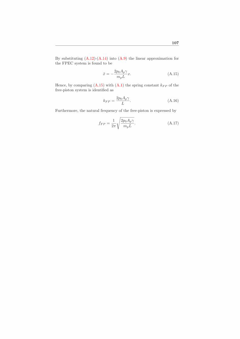
107
By substituting (A.12)-(A.14) into (A.9) the linear approximation forthe FPEC system is found to be
x = −2p0Apγ
mpLx. (A.15)
Hence, by comparing (A.15) with (A.1) the spring constant kFP of thefree-piston system is identified as
kFP =2p0Apγ
L. (A.16)
Furthermore, the natural frequency of the free-piston is expressed by
fFP =1
2π
√
2p0Apγ
mpL. (A.17)


Appendix B
Longitudinal Vehicle
Dynamics
B.1 Vehicle Model
A vehicle must overcome resistive forces caused by the environment tobe able to move. The equations describing this are usually referred toas the longitudinal dynamics of the vehicle. The three major resistiveforces are:
• Aerodynamic drag Fd, due to the viscous friction of the surround-ing air.
• Rolling resistance Fr, due to the friction between the tires andthe road.
• Road grading Fg, due to gravity when driving uphill or downhill.
The vehicle’s longitudinal motion can be described using Newton’ssecond law
mvdv(t)
dt= Ft − (Fd + Fr + Fg), (B.1)
where mv is the vehicle mass and Ft is the net traction force providedby the vehicle’s traction engine.
B.1.1 Aerodynamic Drag
The aerodynamic resistance is caused by viscous friction of the sur-rounding air and by the pressure difference between front and rear ofthe vehicle [28]. If the vehicle is assumed to be a prismatic body theresistive force can be expressed as
Fd(v) =1
2ρairAfCdv
2, (B.2)
109

110 Appendix B. Longitudinal Vehicle Dynamics
where ρair is the air density, Af is the vehicle frontal area, v is thecurrent speed and Cd is the coefficient of drag originating from theaerodynamic properties of the vehicle. As seen, in (B.2) the drag forcedepends quadratically on the speed v, hence it will make a large con-tribution at high speeds. It can also be concluded that decreasing thefrontal area Af or improving the aerodynamic properties, thus decreas-ing Cd, reduces the air friction loss.
B.1.2 Grading Resistance
The resistive force Fg originating from driving on non-horizontal roadsis a function of the roads inclination angle β, the vehicle mass mv andthe gravitational acceleration g
Fg = gmv sinβ. (B.3)
However, in the analysis in this thesis the road is assumed to be flat atall times, thus this force will not be considered.
B.1.3 Rolling Resistance
The rolling resistance is a result of deformation processes between thetire and road surface [2]. This resistance is usually modelled as a con-stant force that depends linearly on the speed, the coefficient of rollingresistance Cr, the vehicle mass mv and the gravitational acceleration g
Fr = Crmvg. (B.4)
In Figure B.1 a comparison of the resistive forces for the vehicle inthis study is given. It can be concluded that the rolling resistance is thelargest resistive loss until the vehicle reaches approximately 70km/h.For higher speeds the drag force is dominating.
B.2 Acceleration Parameters
The power, torque and angular velocity at the wheels can be foundfrom the tractive force Ft if the wheel radius rwheel is known. Thepower Pwheel at the wheels when the vehicle is moving with the speedvacc is
Pwheel = Ft · vacc. (B.5)
The angular velocity ω of the wheel shaft is
ω =vacc
rwheel. (B.6)

B.2. Acceleration Parameters 111
0 50 100 1500
100
200
300
400
500
600
700
800
Speed [km/h]
Resis
tance forc
e [N
]
Aerodynamic friciton
Rolling resistance
Figure B.1: Rolling and aerodynamic resistance for the Prius power-train.
When the two above parameters are known the torque at the wheelscan be expressed as
Twheel =Pwheel
ω. (B.7)
Consequently, by using the descriptions of the resistive forces (B.2)-(B.4), Newton’s second law (B.1), and (B.5)-(B.7) the torque, angularvelocity and power at the wheel shaft can be found. These values canthen be used to calculate, for example, the power into the transmissionor the required torque, speed and power from the electrical machine.


Minimizing Power Pulsations in a
Free Piston Energy Converter
Published in: Proceedings of the 11th EuropeanConference on Power Electronics and
Applications(EPE05)
Dresden, Germany, September 2005


Minimizing Power Pulsations in a Free Piston Energy Converter
Jörgen Hansson, Mats Leksell, Fredrik Carlsson
Dept. of Electrical Engineering, Royal Institute of Technology
Teknikringen 33, SE-100 44 Stockholm
Stockholm, Sweden
Tel: +46/(0)8 - 790.77.75
Fax: +46/(0)8 - 20.52.68
E-mail: jorgen / mats.leksell / fredrikc @ets.kth.se
URL: http://eme.ekc.kth.se
Acknowledgements
The authors gratefully acknowledge funding from the Swedish Energy Agency.
Keywords
«Energy converters for HEV», «Linear drive», «Converter Machine Interactions», «Hybrid ElectricVehicle (HEV)», «Generation of Electrical Energy», «Distributed power», «Emerging technology»
Abstract
A Free Piston Energy Converter (FPEC) is a combination of a linear combustion engine and a linearelectrical machine. This type of converter has many potential advantages like high efficiency, low fuelconsumption and low emissions, which make it suitable for a series hybrid vehicle. However, thegenerated power pulsates due to the reciprocating motion of the translator.
This paper presents a comparative study on how different generator force profiles affect the electricpower pulsations produced by the FPEC. In addition, the influence of these profiles on translatormotion and the needed power converter current is investigated.
A dynamic free piston model is used for the investigation. Results show that the generator force profilehas a major impact on the power pulsation amplitude and peak current demand. Thus the chosen forceprofile will affect dimensioning of power converter, electrical machine and energy storage.Furthermore, loading the translator heavily in the beginning or end of the stroke seems to affect thepeak translator velocity more than evenly distributed load profiles.
Introduction
With the raising oil prices, the debate on fossil fuels and the harder environmental legislationsalternative drivetrains and engines are gaining more interest. The Free Piston Energy Converter (FPEC)is an alternative with potential to be both environmental friendly and efficient. During recent yearsresearch around free piston engines has increased and several prototypes have been built [1–4].
Most work concerning FPECs has focused separately on the mechanical parts of the converter, thecombustion process, [5, 6], linear generator design [7] or control [8]. There has been little research atsystem level of the FPEC. To optimize system performance and reduce size and cost such investigationsare necessary.
One important system issue is the interaction between the generator force, the translator dynamics, andthe drive system. The generator force affects the size of the supplying power converters, the size of theelectrical machine, the amplitude of the generated power pulsations and thus the size of energy storage.This makes the force a critical parameter for system design and performance.

Earlier work in this area have been done by [9] who have investigated how different current and speedprofiles in an FPEC will affect the system efficiency. Moreover, a parameter study of an FPEC has beenperformed by [10] who suggest that a complex force profile is needed to affect the motion of the piston.
This paper investigates what could be gained by varying the force over time. It also examines theinfluence of force profile on the supplying power converter dimensioning and amplitude of powerpulsations. Furthermore, it studies how translator motion is affected by the force.
The Free Piston Energy Converter
Air intake
Exhaust pipe
Fuel injector
MagnetsStator windingValve
Figure 1: A Free Piston Energy Converter
A Free Piston Energy Converter is a combination of a linear combustion engine and a linear electricalmachine converting chemical energy into electrical. A translator with pistons at each end is placedbetween two opposing combustion chambers as seen in Fig. 1. Combustion makes the translatorreciprocate in an almost resonant way and a permanent magnetized linear electrical machine convertssome of the translator’s kinetic energy to electrical. The electrical machine is supplied by a switchmode power converter.
The features of the free piston energy converter are as follows:
• The electrical machine can be used as a motor to start and stop the translator, as a generator forenergy conversion and as an actuator to control the combustion.
• There is no crankshaft constraining the translator motion, which enables variable compression.This makes HCCI possible, a promising combustion process where the air-fuel mixture is selfignited when the pressure and temperature are sufficient. This process has almost 50% chemicalto mechanical conversion efficiency [6]. In addition, the emissions, especially of nitrous oxides(NOx) and particulate matter (PM), are very low.
• The variable compression ratio in combination with HCCI makes it possible to utilize differentfuels with minor hardware changes [5].
• The energy converter can be started and stopped very fast, and change rapidly between differentpower levels, which will minimize the use of a battery if used in a drivesystem [11].
• The system is compact, modular and has high power density.
These features make it very suitable as a power unit in a series hybrid vehicle. In fact, using a freepiston energy converter in a heavy duty application hybrid may reduce fuel consumption up to 25%[12]. Other possible applications could be auxiliary power units and distributed generation.
Power pulsations
The translator velocity and thus the delivered power reaches zero towards the end of the stroke. As aresult the delivered power pulsates. These pulsations introduce issues that must be considered:
• The supplying power converter must be dimensioned to handle the pulsations.

• If the converter is used in a vehicle the pulsations can introduce torque ripple in the propellingelectrical machine. To smoothen these pulsations an energy storage device could be used.Another solution is to overdimension the propelling electrical machine so it acts as an electricalflywheel. But to optimize size, cost and performance of the used components it is desirable not tohave larger pulsations than necessary.
The amplitude of the power pulsations is determined by the translator velocity and the generator force.As the free piston system is almost resonant, the velocity will not change significantly with differentforce profiles. This could potentially be utilized to reduce the amplitude of the power by controlling theforce the correct way.
Force profiles
To generate electric energy the force from the generator is doing work on the translator. The generatorforce is proportional to the current so the peak force decides the peak current the supplying powerconverter must be able to deliver. However, the same work, W , over the same distance can be doneusing different shapes of force, F(x), in accordance with the integral
W =
∫
F(x)dx, (1)
where x is translator position. This means that doing the same work using for example a triangular forceshape, compared to a rectangular one, twice the peak force and thus twice the peak current is needed.The question is what could be gained by using different profiles. Possible load control goals could be:
• Loading the translator more at the beginning of the stroke which results in more time for faulthandling and motion control.
• Loading the translator late in the stroke to utilize more of the kinetic energy for compression.
• Reducing power pulsations.
• High efficiency by using a force profile similar to the velocity profile [9].
• Minimizing the components.
These goals are in conflict with each other and will put different requirements on the converter andelectrical machine performance. In this study the force profiles described below and seen in Fig. 2 areinvestigated to see if the goals can be fulfilled.
Profile 1: Rectangular
Loading the generator using a constant force is a simple way of controlling the system. As this resultsin a rectangle, the lowest current of all profiles investigated is needed.
Profile 2: Inverse velocity
The power delivered is proportional to the translator velocity times the force. Using a force that ideallyshould be the inverse of the speed results in a square power profile. This could reduce the powerpulsations. To limit the peak force an approximation of the velocity inverse is used here.
Profile 3: Sinusoidal left
A sinusoidal profile starting with lower values.
Profile 4: Sinusoidal right
A sinusoidal profile starting with higher values.

−0.05 0 0.050
5
Gen. fo
rce [kN
]
Transl. position [m]
Profile 1
−0.05 0 0.050
5
Gen. fo
rce [kN
]
Transl. position [m]
Profile 2
−0.05 0 0.050
5
Gen. fo
rce [kN
]
Transl. position [m]
Profile 3
−0.05 0 0.050
5
Gen. fo
rce [kN
]
Transl. position [m]
Profile 4
−0.05 0 0.050
5
Gen. fo
rce [kN
]
Transl. position [m]
Profile 5
−0.05 0 0.050
5
Gen. fo
rce [kN
]
Transl. position [m]
Profile 6
−0.05 0 0.050
5
Gen. fo
rce [kN
]
Transl. position [m]
Profile 7
−0.05 0 0.050
5
Gen. fo
rce [kN
]
Transl. position [m]
Profile 8
Figure 2: Generator force as a function of translator position when the translator is moving from left toright.
Profile 5: Trapezoid
The force can not reach maximal value instantaneously as assumed in the rectangular case; a trapezoidprofile could be closer to reality. Furthermore, the translator velocity over time is similar to a trapezoid,which results in high efficiency when using trapezoidal current [9].
Profile 6: Half sinusoidal
Using this half-period sinusoidal profile may also result in high efficiency as it resembles the translatorvelocity [9].
Profile 7: Triangular left
A left triangular profile is used to investigate the effect of reducing much of the translator kineticenergy in the beginning of the stroke. Using this triangle, 75% of the total work is done within the firsthalf of the stroke.
Profile 8: Triangular right
To investigate the influence of loading the generator more at the end of the stroke a right triangularprofile is used. In contrast to the triangular left profile only 25% of the work is done within the first halfstroke.
System modeling
To study the influence of force on the translator movement, a dynamic model of the free piston isneeded. The motion of the piston is mainly determined by the combustion process and the generatorforce which means that both of these must be taken into account. However, a simplified model of thecombustion process will still capture the main translator motion and is therefore sufficient for thisstudy. Several papers suggest these types of simulation models and most approaches are quite similar.In this study the one suggested by [5] is used and described below.
Thermodynamics
The first law of thermodynamics and the ideal gas law are used to derive dynamic equations forpressure and temperature in each cylinder. Assuming the mechanical work done to be volume work theincylinder pressure and temperature can be expressed by
d p
dt=
∂Q
dt
p
mcvT−
γp
V
dV
dt(2)

dT
dt=
1
mcv
∂Q
dt+
T (1− γ)
V
dV
dt(3)
where V is cylinder volume, T cylinder gas temperature, p cylinder pressure, m gas mass, Q heat, cv isthe specific heat with constant volume and γ is the ratio of specific heats.
Mass fraction burned
When the air/fuel mixture ignites it burns for a while, the mass fraction burned is modeled using aWiebe function,
xb = 1− e−a
(t
td
)N+1
, (4)
and the heat released during combustion is
∂Q
dt= Qin
dxb
dt, (5)
where xb is the mass fraction burned. Qin is the total heat added during one combustion, td is theduration of combustion and τ is the time since combustion started. The constants N and a are used toform the shape.
Ignition delay
The combustion does not start instantaneously when the pressure and temperature in the combustionchamber are high enough, but is delayed until the integral
∆(τ) =
t+τ∫
t
1
Apne
EART dt (6)
reaches the value one. Ea is a fuel dependent constant, R is the universal gas constant and τ is the timeelapsed since fuel injection.
Heat transfer
During combustion not all heat generated is converted into work, losses to the cylinder walls occur inaccordance with
∂Qht
dt= αA(T −Tw) (7)
α = 130V−0.06( p
105
)0.8T−0.4(Up + 1.4)0.8, (8)
where Tw is the cylinder wall temperature and Up is the piston mean velocity. This model is valid forregular diesel engines and will overestimate the heat loss in a HCCI engine.
Electrical machine
Almost no power is delivered close to the translator turning points as the velocity, thus the inducedelectromotive force, reaches zero. Therefore the generator is not loaded around these points. Thisresults in a machine model
Fel = Fre f when |x| < xel
Fel = 0 when |x| > xel . (9)

The direction of the force is always opposite to the piston velocity. Furthermore, a constant electricalmachine efficiency of 94% is assumed.
Translator motion
Finally, the piston motion is described using Newton’s second law,
mp
dv
dt= Fel + Ap(p1 − p2). (10)
where mp is translator mass and Ap is piston area.
Control system
+
+
-
-
Power
Ignition Timing
Controller
Controller
P_el
P_ref
t_ign_refF_el
Q_comb
RG
A
t_ignition
FPEC
Figure 3: FPEC control system
The HCCI process in combination with the FPEC is a complex, unstable, multiple input multiple outputprocess, challenging to control. In this investigation a simple control system used for initial studies by[1] is utilized.
A block diagram of the control system is seen in Fig. 3. Using generator force amplitude and air/fuelmixture as control signals, two PI controllers control ignition delay and mean power output. The controlsignals are decoupled using a Relative Gain Array (RGA) with values determined from open-loopsimulations. The controller is event trigged using translator direction change. This control systemwould not be applicable on a real FPEC system since only one sample each stroke is taken which wouldbe too slow for advanced combustion control. However, it is sufficient for this investigation.
FPEC data
The FPEC used in the simulations has a translator weight of 9 kg, a bore of 100 mm and a maximumpower of 45 kW.
Simulation and results
The system is modeled using Matlab/Simulink. Simulations using the eight different force profiles areperformed until the system reaches steady state. The power control reference is set to 20 kW. Thesimulation results are presented in Table 1.
Table 1: Simulation results
1 2 3 4 5 6 7 8
Ppeak [kW] 28.5 25.5 33.2 30.9 43.6 44.4 46.8 39.0Fpeak [kN] 2.9 5.0 3.4 3.4 4.3 4.5 5.9 5.4vpeak [m/s] 10.6 10.6 10.5 10.7 10.9 10.9 9.9 11.2fpower. [Hz] 65.0 65.0 64.0 65.0 64.0 64.0 61.0 67.0Work [J] 329.0 328.0 332.0 328.0 330.0 330.0 339.0 312.0

Typical position, speed and acceleration curves from simulation can be seen in Fig. 4. Note that thevelocity over time resembles something between a sinusoid and trapezoid which was the motivation forthe high efficiency profiles 5 and 6.
0 10 20 30 40
−10
−5
0
5
10
15
time [ms]
Translator motion
Displacement [cm]
Velocity [m/s]
Acceleration [km/s2]
Figure 4: Typical free piston displacement, velocity and acceleration from simulation.
The peak current is assumed to be proportional to the peak force. As relative values are moreinteresting for comparison, the achieved simulation results are normalized. That is the peak powerlevel, peak current, and work from each simulation case is divided with the corresponding result fromthe rectangular profile. A barchart of the normalized values is presented in Fig. 5.
1 2 3 4 5 6 7 80
0.5
1
1.5
2
| Peak Power | Peak current | Work |
No
rma
lize
d v
alu
e
Peak power
Peak current
Work
Figure 5: Normalized peak power amplitude, peakcurrent, and work.
−0.08 −0.06 −0.04 −0.02 0 0.02 0.04 0.06 0.08−15
−10
−5
0
5
10
15
Position [m]
Ve
locity [
m/s
]
Velocity as function of position
Figure 6: Translator velocity as a function of posi-tion.
The velocity as a function of translator position in steady-state can be seen in Fig. 6. Six of the curvesare essentially the same but two extreme cases, corresponding to the triangular force profiles 7 and 8,occur. In these two cases the total work done differs slightly from the other simulation cases. The peakvelocity is 10% lower with only 3% higher work done for the early load force profile. For the late loadcase, the peak velocity has increased by 5% decreasing the work by the same amount. Increasedfrequency with lower load and vice versa is consistent with the work presented in [10].
Loading the translator early or late in the stroke seems to have more effect on the translator dynamicsthan other load strategies. However, looking at the peak current demand for these two profiles in Fig. 5almost twice the peak current compared to the rectangular case is needed and the power pulsations havehigh amplitude.
It can also be seen in Fig. 5 that the inverse velocity force (profile 2) results in the lowest powerpulsations but 70% higher peak current demand compared with a constant force. Thus power pulsationscan be somewhat reduced by generator force control, again at the price of a large peak current.
As expected, a constant force (profile 1) demands the lowest current, and it also results in quite lowpower pulsations.

Conclusions
Simulation results shows that the generator force has major influence on power pulsation amplitude.When choosing force control strategy this must be taken into account since large pulsations will requirelarge components. Moreover, goals like reduced power pulsations or improved translator control can befulfilled but at the price of a high peak current demand.
This study has not covered combustion issues. Translator motion and position relative to ignition willaffect the combustion process and thus emissions and efficiency. Furthermore, when using a highbandwidth control system, which updates several times during a stroke and considers both combustionand translator motion, an exact force profile can probably not be chosen in advance. But the controlsignal could still end up in a profile similar to the ones investigated here.
To conclude, the results provided here give an insight into how force control strategies will affectnecessary performance of converter, electrical machine and energy storage. High peak current demandsand power pulsations can be coped with, but it is important to consider them when designing the systemto achieve an efficient system with a reasonable size and cost. This is especially important if the FPECis placed in a vehicle application, as low cost and weight are key parameters for the automotive industry.
References
[1] EU founded free piston energy converter project. GRD2-2001-51813.
[2] D. Carter and E. Wechner. The free piston power pack: Sustainable power for hybrid electricvehicles. SAE Technical Paper 2003–01–3277, 2003.
[3] M. Prados. Towards a linear engine. Master’s thesis, Stanford University, 2002.
[4] P. V. Blarigan. Advanced internal combustion research. In Proceedings of the 2002 U.S. DOE
Program Review, 2002.
[5] J. Fredriksson. The Free Piston Engine – The Automotive Prime Mover of the Future. Licentiatethesis, Chalmers University of Technology, 2004.
[6] A. Kleemann, J. Dabadie, and S. Henriot. Computational design studies for a high-efficiency andlow-emissions free piston engine prototype. SAE Technical Paper 04FFL-39, 2004.
[7] W. M. Arshad. A Low-Leakage Linear Transverse-Flux Machine for a Free-Piston Generator.PhD thesis, Royal Institute of Technology, Stockholm, Sweden, 2003.
[8] T. A. Johansen, O. Egeland, E. A. Johannessen, and R. Kvamsdal. Dynamics and control of afree-piston engine. ASME Journal of Dynamic Systems, Measurement and Control, 125,September 2003.
[9] Y. Liu, W. M. Arshad, M. Leksell, and P. Thelin. Influence of speed and current profiles uponconverter dimensioning and electrical machine performance in a free-piston generator. InProceedings of the 4th international Symposium on Linear Drives for Industry Applications,LDIA, Birmingham, England, 2003.
[10] C. Atkinson, S. Petreanu, N. N. Clark, R. J. Atkinson, T. I. McDaniel, S. Nandkumar, andP. Famouri. Numerical simulation of a two-stroke linear engine-alternator combination. SAE
Technical Paper 1999-01-0921, 1999.
[11] E. Max. FPEC, Free piston energy converter. In Proceedings of the 21st Electric Vehicle
Symposium & Exhibition, EVS 21, Monaco, 2005.
[12] A. Cosic, J. Lindbäck, W. M. Arshad, M. Leksell, P. Thelin, and E. Nordlund. Application of afree piston energy converter in a series hybrid vehicle. In Proceedings of the 4th internationalSymposium on Linear Drives for Industry Applications, LDIA, Birmingham, England, 2003.

Operational Strategies for a
Free Piston Energy Converter
Published in: Proceedings of the FifthInternational Symposium on Linear Drives for
Industry Applications(LDIA05)
Kobe-Awaji, Japan, September 2005


Operational Strategies for a
Free Piston Energy Converter
Jorgen Hansson∗†, Mats Leksell∗, Fredrik Carlsson∗ and Chandur Sadarangani∗
∗Royal Institute of Technology, Departement of Electrical EngineeringTeknikringen 33, SE-100 44 Stockholm, SWEDEN,Phone +46-(0)8-790-7775, Facsimile +46-(0)8-205268
Email:†[email protected]
AbstractThis paper investigates how the losses in a Free Piston Energy Converter during start, stop and idling
affects energy consumption and required power from the supply system.Simulation results indicate that the electrical machine efficiency is the most critical factor during start.
Moreover, by choosing the correct amplitude of the starting force, energy consumption during start can bereduced. When it comes to idling, friction is the most significant loss factor. Nevertheless, by compensatingthe mechanical loss for short time intervals using the generator force, the reciprocating motion can be keptalive for a rapid start without major energy consumption.
Keywords: energy conversion, hybrid vehicle, Free Piston Energy Converter, auxiliary power unit, energy, power,HCCI
1. Introduction
As the world is reaching the peak of oil production,the oil prices are rising and the environmental legisla-tions for vehicles are getting harder there is a rising in-terest in alternative drivetrains and engines which canreduce fuel consumption and emissions. The Free Pis-ton Energy Converter (FPEC) is such an engine, whichconverts chemical energy to electrical. The intended ap-plication for the FPEC is as a power unit in a serieshybrid vehicle.
A hybrid electric vehicle’s (HEV) performance is verydependant on the vehicle’s energy management strat-egy. In fact, controlling the energy sources inappropri-ate may increase emissions and lower the system effi-ciency compared to a conventional vehicle. Therefore,to make efficient use of the FPEC in a HEV it is desir-able to know which operational mode the FPEC shouldbe in and what cost that mode is associated with. Fur-thermore, to design the supplying electrical system foroptimal performance, the required energy and power foreach mode must be known.
This paper studies the operational modes which arethe most essential for a vehicle application with the ex-ception of running: start, idling and to some extent stop.The associated cost will be energy consumption. More-over losses, required power and time issues are consid-ered.
2. Free Piston Energy Converter
The Free Piston Energy Converter consists of a linearelectrical machine placed between two opposing com-bustion chambers as seen in Fig. 1. Combustion in thechambers makes the translator reciprocate and generateelectrical energy.
Exhaust valve Intake port
Fuel Injector
Magnets Stator winding
Translator Piston
Combustion chamber
Fig. 1. Cross section of a Free Piston EnergyConverter
As no crankshaft is limiting the translator motionthe compression in the cylinders can be varied. Thismakes a modern combustion technique called Homoge-nous Charge Compression Ignition (HCCI) possible. Inthis combustion process the air-fuel mixture is injectedat the beginning of the stroke and compressed until igni-tion, hence the name. HCCI has an indicated efficiencyaround 50%, low fuel consumption and low emissionsespecially of NOx and particulate.
One of the drawbacks of linear engines and HCCI hasbeen that both the combustion process and the transla-tor motion are harder to control than in a conventionalengine. However, with the FPEC the electrical machinecan be used as an extra actuator to improve controlla-bility of the system.
During recent years the interest in FPECs has grownand prototypes have been built. One contribution canbe seen in Fig. 2.
3. Operational modes
As there is a choice between idling and a stop fol-lowed by a start, it is useful to have some cost associatedwith these operational modes to know which to utilize.In this study energy consumption has been chosen butother costs could be emissions or fuel consumption.
3.1 Start-up The start scenario investigated isto inject the air-fuel mixture, close the exhaust valves

Fig. 2. Free Piston Energy Converter prototypedeveloped in (3) (4) .
and use the electrical machine force to move the trans-lator back and forth until the mixture ignites. Ignitionis dependant on several parameters, the two most im-portant are: pressure and temperature. However, it isnot sufficient just to reach the required level of temper-ature and pressure. In addition this level or higher mustbe kept for a while to make the mixture ignite. Thatis, if the required levels of pressure and temperature arepassed early in the stroke, they will rise further and themixture may ignite. On the other hand, if the requiredlevel is reached near the end of a stroke, there may notbe enough time for the mixture to ignite and one addi-tional stroke is necessary.
A desirable starting procedure should be rapid so nomajor delay is noticed before power is delivered fromthe generator. At the same time, the power requiredto start should not exceed the rated values of the sup-plying components. Furthermore, a low energy demandmay increase the total system efficiency.
Using closable intake valves or not will also affect thestart strategy. If the valves are not closable the air-fuelmixture may be diluted if too many strokes are neededfor ignition during start-up.
3.2 Idling Idling mode can be useful if the powerdemand is low only for a short while and a rapid start-upis desired. From an emission point of view idling mayalso be favorable, as a transient start-up of a combustionengine usually results in high emissions.
When idling is required the fuel injection is stoppedand the exhaust valves is closed, forcing the translatorto bounce back and forth on the gases in the cylinders.This mode is very dependant on the mechanical lossesin the system as they are the energy reducing factor.Nevertheless, if idling is a desirable mode, it would bepossible to maintain a reciprocating translator motionwithout combustion by cancelling out the mechanicallosses using the generator force.
3.3 Stop When the system is stopped, time isnot an issue but as much energy as possible should beregenerated and stored for a good energy economy. Asfriction and other losses will reduce the translator kineticenergy over time a rapid stop is desirable.
The available electrical force acting on the translatoris not sufficient to stop the translator in one stroke, thusat least two strokes is required before the translator isdrained of all energy.
4. System modeling
To investigate the operational modes a dynamic sim-
Velocity [m/s]
Fo
rce
[N
]
0 5 10 15 20 25 300
500
1000
1500
2000
2500
3000
3500
4000
0.75
0.8
0.85
0.9
0.95
Fig. 3. Efficiency map (3) for the electrical machinewith working points for each start-up case.
ulation model of a 45 kW FPEC is implemented usingMatlab/Simulink. Reference (1) and (2) suggest modelsof Free Piston Engines and in this paper a similar ap-proach is used.
The gas in the cylinders is assumed to be ideal,
piVi = mgRTi, · · · · · · · · · · · · · · · · · · · · · · · · · · · · · · (1)
and the compression is assumed to be polytropic,
piVγi = const. · · · · · · · · · · · · · · · · · · · · · · · · · · · · · · · (2)
These two assumptions hold if the pressure is not toohigh. In (1)-(2) γ is the specific heat ratio, mg is thegas mass, pi is cylinder pressure, Vi is cylinder volume,R is the universal gas constant and Ti is the gas tem-perature. By using Newton’s second law and adding thelosses described below the differential equations shownin appendix 1 can be derived.
5. Losses
The most significant loss factors during start and stopwill probably be friction and electrical machine effi-ciency. However, as this is a combustion engine the heattransfer to the cylinder walls is also considered.
5.1 Electrical machine efficiency The electri-cal machine efficiency is modelled using an efficiencymap from (3). However, when starting from standstillthe losses in the electrical machine will probably be veryhigh the first milliseconds due to inertia, transient cur-rents etc. Therefore, the electrical machine efficiencyis assumed to be only 25% during the first stroke. Forthe following strokes it is taken from the efficiency mapgiven in Fig. 3.
5.2 Heat transfer to walls Some of the heatgenerated will leak out through the cylinder walls andthus delay the ignition. This heat transfer is mainly de-pendent on the temperature difference between the gasand the cylinder walls. However, during start-up thistemperature difference will not be as big as during com-bustion. Consequently, the heat transfer will not be amajor loss. Here the heat transfer is modelled accordingto Hohenberg (1):
∂Qloss
dt= αAp(T (t) − Tw(t)) · · · · · · · · · · · · · · · · · · · · · · · · (3)
α = 130V (t)−0.06
(p(t)
105
)0.8
T (t)−0.4(Vp + 1.4)0.8(4)

Vp is the piston mean velocity, Tw is the cylinder walltemperature, Qloss is the heat loss and Ap is the pistonarea.
5.3 Friction Friction is an essential parameterespecially if the FPEC is in idling mode. As this willbe the major loss factor, the size of the friction workwill determine how long the system can reciprocate be-fore reaching standstill.
Few empirical results are available for this type ofengine, therefore friction is hard to predict. However,as the crankshaft mechanism is eliminated the frictionshould be quite low and originates from the friction be-tween the cylinder wall and the piston skirt and pistonrings (2).
Reference (1) and (2) have utilized a model for a two-stroke engine with rolling element bearings and it is alsoused in this investigation. Since the shape of the frictionforce is unknown it is modelled using the Friction MeanEffective Pressure (FMEP) which is a mean value overthe stroke.
FMEP =Wf
Vd· · · · · · · · · · · · · · · · · · · · · · · · · · · · · · (5)
Wf = Ff2Lstroke · · · · · · · · · · · · · · · · · · · · · · · (6)
Wf is the friction work, Vd is the displaced cylinder vol-ume and Lstroke is the stroke length. The FMEP canalso be expressed as
FMEP = 6300Lstrokef · · · · · · · · · · · · · · · · · · · · · (7)
where f is the translator frequency. Combining (5)–(7)results in a mean friction force described by
Ffric =6300
2Vdf. · · · · · · · · · · · · · · · · · · · · · · · · · · · (8)
5.4 Model characteristics Implemented in thesimulation model are two other characteristics that mayaffect the result.
• Intake ports cannot be closed. As a result the cylin-der pressure takes the outer pressure value everytime the translator is uncovering the port. Thisintroduces losses if the cylinder pressure is higherthan the outer pressure at that time. However, sim-ulations with closed inlet ports indicate no majordifference in required energy and power for start.
• When the translator is reversing almost no power isdelivered, therefore the generator force cannot loadthe translator near the turning points.
6. Results and discussion
6.1 Start Start of the FPEC using a constantforce from 400 N–4000 N was simulated. Forces lowerthan 400 N were investigated initially; however, start-upbecame impossible for these cases as the friction forceeventually exceeded the generator force.
Furthermore, it is assumed that an ignition can beginwhen the pressure rises above 35 bar and the tempera-ture above 700 K. Just reaching these levels may not besufficient as discussed earlier. Therefore the time withpressure and temperature above the desired levels wasrecorded.
0.5 1 1.5 2 2.5 3 3.5 40
0.5
1
1.5
Generator force [kN]
En
erg
y [
kJ]
15
10 8 7 6 5 4 4
4 3
3 3
3 3
3
2 2 2 2 2 2 2 2 2 2 2 2 2 2 2 2 2 2
1 1 1 1
IdealFriction lossElectrical machine loss
Fig. 4. Required electrical energy to start a com-bustion. Full bar is total energy consumption. Therequired number of strokes is presented above thebars.
0.5 1 1.5 2 2.5 3 3.5 40
10
20
30
40
50
60
70
80
90
Generator force [kN]
Po
we
r [k
W]
1510 8 7 6 5 4 4 4 3 3 3 3 3 3 2 2
2 2
2 2
2 2
2 2
2 2
2 2
2 2
2 2
1 1
1 1
IdealFriction lossElectrical machine loss
Fig. 5. Required peak electrical power to start acombustion. Full bar is total peak power. Therequired number of strokes is presented above thebars.
It can be seen in Fig. 4 that every time the requirednumber of strokes to start combustion decreases so doesthe required energy. Consequently, the energy consump-tion can be minimized for a desired number of strokes.Furthermore, the total friction loss decreases with higherforce and thus shorter start-up time. In fact it only hasa minor influence for a two stroke or faster start-up. Theheat loss during start is negligible and cannot even bediscerned in the bars. This was an expected result dueto the low temperature difference as discussed earlier.
The required power increases with shorter start-uptime as seen in Fig. 5. The electrical machine efficiencyhas major effect on the required power. For a genera-tor force over 2700 N the power exceeds 45 kW whichis the maximal power of the FPEC. As the supplyingsystem has to manage 45 kW, using a start power up tothis level is acceptable, but it is not desirable to designthe system for higher powers just to be able to start.However, the assumption of only 25% electrical machineefficiency the first ms affects the result heavily for thehigh-force cases and may be too pessimistic.
The time for start-up is presented in Fig. 6. It can beseen that for the same number of strokes no major timeimprovement is made by using a larger force. This sup-ports the conclusion that the lowest possible force for adesired number of strokes should be used for low energyconsumption.
A realistic scenario could be a two-stroke start-up sce-nario which results in a start time of approximately50 ms. However, the time with required ignition level

0.5 1 1.5 2 2.5 3 3.5 40
50
100
150
200
250
300
350
400
450
Generator force [kN]
Tim
e f
or
sta
rtu
p [
ms]
15
10
8 7
6 5
4 4 4 3 3 3 3 3 3
2 2 2 2 2 2 2 2 2 2 2 2 2 2 2 2 2 2 1 1 1 1
Fig. 6. Time to reach ignition level. The requirednumber of strokes is presented above the bars.
0.5 1 1.5 2 2.5 3 3.5 40
0.5
1
1.5
2
2.5
Generator force [kN]
Tim
e a
bo
ve
le
ve
l [m
s]
1510
8 7
6 5
4
4
4
3
3 3
3 3 3
2
2
2 2
2 2 2 2 2 2 2 2 2 2 2 2 2 2
1
1
1 1
Fig. 7. Time with pressure and temperature aboverequired level for ignition. The required number ofstrokes is presented above the bars.
Table 1. Initial values for idling simulation.
p1 4.7 [MPa] p2 0.12 [MPa] x0 -6.3 [cm] a0 4000 [m/s2]
T1 977 [K] T2 360 [K] v0 0 [m/s]
is quite small for the first two-stroke case as seen inFig. 7. Hence, a larger start-up force may be necessaryto assure ignition.
6.2 Idling The simulation is started using theinitial values shown in Table. 1 which corresponds toa 29kW working point. A combustion has just occurredin cylinder 1, the velocity is zero and the acceleration ishigh as the translator has just reversed.
The friction force, during the first stroke after combus-tion, is approximately 330 N and a friction work of 42 Jis done. Consequently, the translator motion can be keptalive at an operating point near the FPEC rated powerof 29 kW by pushing the translator with a force of 330 N.Doing this with a frequency of 60 Hz over a distanceof 12 cm results in a energy consumption of 2400 J/sfor idling. On the other hand, looking at the requiredenergy to start in Fig. 4 it spans from 500–1300 J forthe cases investigated. Therefore, idling for long time-intervals may not be efficient from an energy point ofview. However, it may not be necessary to idle near thisworking point. Decreasing the reciprocating frequencyduring idling would lower the friction force and thus therequired energy. This would still result in high efficiencyas the electrical machine efficiency (Fig. 3) is acceptableover a large area. When deciding on a good idling work-ing point combustion issues should also be consideredand it is not the aim of this investigation.
It should be noted that the idling scenario’s numericalresult is heavily dependant on the friction model. Butas the start-up scenarios use the same friction model thelosses will be proportional and a comparison betweenthese two modes is possible.
6.3 Stop When running stationary at 29 kW themaximal translator velocity is approximately 11 m/swhich results in a kinetic energy of
Wk =mv2
2≈ 544J. · · · · · · · · · · · · · · · · · · · · · · · · · (9)
Consequently, this is the maximal energy that can beregenerated from the FPEC during a stop from this op-erating point.
7. Conclusions
Heat loss, and friction seems to have minor effect onthe required start-up power and energy levels due to therapid start-up time. Moreover, the required energy andpower for start can be minimized by choosing the min-imal force necessary for a desired number of start-upstrokes. Furthermore, idling for long time intervals maybe costly from an energy point of view.
It is planned to validate some of the results providedhere on the prototype developed in (4).
References
( 1 ) Jakob Fredriksson. The Free Piston Engine – The Automo-
tive Prime Mover of the Future. Licentiate thesis, Chalmers
University of Technology, Gothenburg, Sweden, 2004.
( 2 ) C.M. Atkinson, Sorin Petreanu, Nigel N. Clark, Richard J.
Atkinson, Thomas I. McDaniel, Subhash Nandkumar, and
Parvis Famouri. Numerical simulation of a two-stroke linear
engine-alternator combination. SAE Technical Paper 1999-
01-0921, 1999.
( 3 ) Erland Max. FPEC, Free piston energy converter. In Proceed-
ings of the 21st Electric Vehicle Symposium & Exhibition,
EVS 21, Monaco, 2005.
( 4 ) GRD2-2001-51813. EU founded free piston energy converter
project.
Appendix
1. ModelingSubscript i refers to cylinder one or two.
dpi
dt= −
dQloss
dt
pi(t)
mgcvTi(t)−
pi(t)γ
Vi(t)
dVi
dt· · · · · · · · · (A1)
dV1
dt= v(t)Ap · · · · · · · · · · · · · · · · · · · · · · · · · · · · · · · · · · (A2)
dV2
dt= −v(t)Ap · · · · · · · · · · · · · · · · · · · · · · · · · · · · · · · · (A3)
dv
dt=
Ap
mp(p1(t) − p2(t)) +
1
mp(Fel(t) − Ffric(t))(A4)
dx
dt= v(t) · · · · · · · · · · · · · · · · · · · · · · · · · · · · · · · · · · · · · (A5)
Table A1. Variables and constants used in (A1)–(A5)
pi(t) pressure [Pa] v(t) translator velocity [m/s]
Ti(t) temperature [K] Vi(t) cylinder inner volume [m3]
Fel(t) generator force [N] Ap piston area [m2]
mp translator mass [kg] x(t) translator position [m]
γ specific heat ratio [-] cv specific heat at const. vol. [ J
kgK]

Performance of a Series Hybrid
Electric Vehicle with a Free-Piston
Energy Converter
Published in: Proceedings of the 2006 IEEEConference on Vehicle Power and Propulsion
(VPPC2006)Windsor, U.K., September 2006

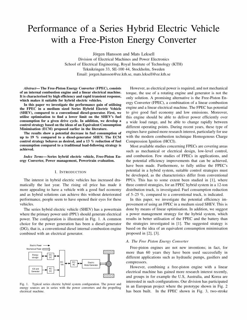
Performance of a Series Hybrid Electric Vehicle
with a Free-Piston Energy Converter
Jörgen Hansson and Mats Leksell
Division of Electrical Machines and Power Electronics
School of Electrical Engineering, Royal Institute of Technology (KTH)
Teknikringen 33, SE-100 44, Stockholm, Sweden
Email: [email protected], [email protected]
Abstract— The Free-Piston Energy Converter (FPEC), consistsof an internal combustion engine and a linear electrical machine.It is characterised by high efficiency and rapid transient response,which makes it suitable for hybrid electric vehicles.
In this paper we investigate the performance gain of utilisingthe FPEC in a medium sized Series Hybrid Electric Vehicle(SHEV), compared to a conventional diesel-generator. First, weutilise optimisation to find a lower limit on the SHEV’s fuelconsumption for a given drive cycle. In addition, we develop acontrol strategy based on the ideas of an Equivalent ConsumptionMinimisation (ECM) proposed earlier in the literature.
The results show a potential decrease in fuel consumption ofup to 19 % compared to a diesel-generator SHEV. The ECMcontrol strategy behaves as desired, and a 13 % reduction of fuelconsumption compared to a traditional load-following strategy isachieved.
Index Terms— Series hybrid electric vehicle, Free-Piston En-ergy Converter, Power management, Powertrain evaluation.
I. INTRODUCTION
The interest in hybrid electric vehicles has increased dra-
matically the last year. The rising oil price has made it
more appealing to have a vehicle with a good fuel economy
and as hybrid solutions can achieve this without deteriorated
performance, people seem to have opened their eyes for these
vehicles.
The series hybrid electric vehicle (SHEV) has a powertrain
where the primary power unit (PPU) should generate electrical
power. The configuration is illustrated in Fig. 1. A common
choice for the power generation has been a diesel-generator
(DG), that is, a conventional diesel internal combustion engine
combined with an electrical generator.
Electric
Motor/Generator
DC-
linkDC/
AC
DC/
DC
AC/
DC
Energy
storage
Electric Power
Mechanical Power
ICE and
Generator
Fig. 1. Typical series electric hybrid system configuration. The power andenergy sources are in series with the power converters and the propellingelectrical machine.
However, as electrical power is required, and not mechanical
torque, the use of a rotating engine and generator is not the
only solution. A promising alternative is the Free-Piston En-
ergy Converter (FPEC), a combination of a linear combustion
engine and a linear electrical machine. The FPEC has potential
to give good fuel economy and low emissions. Moreover,
this engine should be able to deliver power efficiently over
a wide load range, and be able to change rapidly between
different operating points. During recent years, these type of
engines have gained more research interest, particularly for use
with the modern combustion technique Homogenous Charge
Compression Ignition (HCCI).
Most available studies concerning FPECs are covering areas
such as mechanical or electrical design, low-level control,
and combustion. Few studies of FPECs in applications, and
the potential efficiency improvements that can be achieved,
have been made. Furthermore, to fully utilise the FPEC’s
potential in a hybrid system, suitable control strategies must
be developed, as the characteristics differ from conventional
PPUs. This has to some extent been studied in [1], where
three control strategies, for an FPEC hybrid system in a 12-ton
distribution truck, is investigated. Fuel consumption reduction
of 5–25 %, compared to a conventional truck, is indicated.
In this paper, we investigate the potential efficiency im-
provement of using an FPEC in a medium sized SHEV. This is
done by means of linear optimisation. In addition, we suggest
a power management strategy for the hybrid system, which
results in better utilisation of the FPEC and the battery than
the strategies investigated in [1]. The suggested strategy is
based on the idea of an equivalent consumption minimisation
proposed in [2], [3].
A. The Free Piston Energy Converter
Free-piston engines are not new inventions; in fact, for
more than 60 years they have been used successfully in
different applications such as hydraulic pumps, gasifiers and
compressors.
However, combining a free-piston engine with a linear
electrical machine has gained more research interest recently,
and groups in for example the U.S, Australia, and Korea are
interested in such configurations. Our division has participated
in an European project where the prototype shown in Fig. 2
has been built. In the FPEC shown in Fig. 3, two-stroke

Fig. 2. 45 kW FPEC prototype.
Exhaust valveIntake port
Fuel Injector
MagnetsStator winding
TranslatorPiston
Combustion chamber
Fig. 3. Cross section of an FPEC.
combustion makes the translator reciprocate in an almost
resonant way. Electrical power is generated by the integrated
linear electrical machine. The electrical machine is also used
to stabilise the combustion process and for start and stop of
the engine.
The FPEC has several advantages compared to a conven-
tional engine:
• The electrical machine and combustion engine are com-
bined into one single unit, which reduces the size, weight
and number of moving parts compared to conventional
crank engine-generator combinations.
• The compression ratio is variable, as the translator motion
is determined by the forces acting on the pistons and not
by a crankshaft. This makes it suitable for the modern
combustion technique Homogenous Charge Compression
Ignition (HCCI) with high efficiency and very low emis-
sions of NOx and soot.
• The lack of crankshaft and flywheel results in a good
transient response, which makes it possible to change the
delivered power fast.
• The reduced number of moving parts, results in low
mechanical losses and thus high efficiency.
However, it also has issues. The free piston in combination
with HCCI combustion is an highly unstable process that
requires a sophisticated control system. Moreover, due to
the reciprocating motion of the piston, the delivered power
pulsates. These pulsations must be handled somewhere in the
electrical system. One way to reduce them may be by suitable
force control [4].
In addition to low emissions, two features makes the FPEC
appealing for an SHEV powertrain. The system efficiency is
often lower in an SHEV than in other hybrid topologies, due
to the many power conversions. The efficiency of an FPEC,
however, is estimated to be higher than the efficiency of most
PPUs used today, for example a DG as shown in Fig. 4. Thus,
utilising an FPEC should increase the total system efficiency.
Furthermore, the battery pack in an SHEV is often large, as
it must provide the power difference between, for example, a
0 50 1000
0.1
0.2
0.3
0.4
Percent of max. load [%]
Effic
iency
FPEC
Dieselgen.
Fig. 4. Efficiencies from fuel to electrical power to the DC-link for an FPECand a typical diesel-generator
slow combustion engine and the instantaneous traction load.
The FPEC’s fast transient response makes it possible to reduce
the size of the battery pack.
B. Power Management
In a hybrid vehicle several power sources are available, and
the system efficiency is dependent on how these sources are
utilised, the states of the sources, and the path the power flows.
The power management controller1 decides how this should be
performed in the best way in order to satisfy the load demand.
Consequently, it is a key component in the hybrid system and
its decisions affects the system efficiency.
In addition, this controller should often minimise objectives,
such as fuel consumption, driveability or emissions, under
system constraints. These constraints can for example be a
limited rate of change on power generation or how much
energy it should be in the buffers for good lifetime and
efficiency.
To achieve results that do not depend on how good the con-
trol law is designed, many recent studies suggest optimisation
as a tool for powertrain evaluation. By choosing powerflow as
optimisation variable, the result is independent of the control
law.
In this study, we have used a linear programming (LP)
approach, similar to the one suggested in [5], to find the
best performance of the powertrain. In a linear program the
problem formulation is convex, which results in that the global
optimum, if it exists, is found. Moreover, efficient large-
scale solvers are available, making it possible to solve large
problems rather fast.
On the other hand, to achieve a convex problem formulation
everything must be described using linear or piecewise linear
functions, which may require approximations. In addition, the
drive cycle is described in discrete time points, which also
may introduce discrepancy from the true solution.
When it comes to real power management in SHEVs,
with a combustion engine-generator combination, two control
strategies are often used:
1) The Duty-Cycle, Thermostat or ON-OFF control strat-
egy [6], [7]. This strategy uses the PPU, operating at
a working point with high efficiency, to recharge the
1The term energy management controller is also common in the literature.

battery to an upper limit when the state-of-charge (SoC)
has decreased to a lower limit. In addition, the PPU
provides extra power to the wheels when the load is
high. Some advanced variants estimates the average
mean traction load, and provides that average power by
duty-cycle the PPU.
2) The load-following strategy [8], where the PPU follows
the power load demand, usually with a rate of change
limit. The PPU’s working point with the highest effi-
ciency for the current power demand is chosen. The
power difference between the PPU and the load, due
to the rate limit, is provided by the energy storage.
Both these strategies are also applicable in an FPEC system
but would not fully utilise its two main features: the rapid
transient response, and the high efficiency over a wide load
range. Using these strategies in an FPEC system has been
investigated in [1], and the results indicate that using the FPEC
over a wider load area, compared to duty-cycle control, has
the greatest potential.
We have studied a more sophisticated method for power
management control, the equivalent consumption minimisation
strategy (ECMS). The first appearance of such a strategy seems
to be in [2]. The ECMS aims to reach a good overall fuel
economy by controlling the power sources so that an equiva-
lent fuel cost at each time step is minimised. Strategies of this
type are intuitive, and have successfully been implemented on
real vehicles [9].
II. SYSTEM MODELLING
The best selling hybrid vehicle on the market today is the
Toyota Prius with over 100 000 vehicles sold in the U.S
during 2005. This indicates that its performance satisfies most
consumers. Therefore, we have chosen to investigate a vehicle
with the same performance as the Toyota Prius. However,
as the Prius powertrain is a combination of a parallel and
a series hybrid system, a pure series hybrid powertrain had to
be designed and sized.
Power sources in the vehicle investigated are an FPEC and
a battery. The FPEC has constraints on available power PFP ,
and power rate of change PFP , and the battery has constraints
on available power Pbatt, and state-of-charge SoC,
0 ≤ PFP ≤ PFPmax (1)
−PFPmax ≤ PFP ≤ PFPmax (2)
−Pbattmax ≤ Pbatt ≤ Pbattmax (3)
30% ≤ SoC ≤ 70%. (4)
The parameter and component data for the vehicle, and the
numerical values for the constraints, can be found in Table II
in Appendix.
For the analysis, dynamics and transient behaviour was not
of interest, therefore we used a backwards simulation model.
In such a model the required power is calculated backwards
through the powertrain from the drive cycle speed, using
component efficiencies, maps and static relationships, which
results in fast simulations.
VehicleDynamics
Gear-box
EM efficiencymap
DC-link
Battery &ConverterEfficiency
v[k] Pdist[k]
PF P [k]
Pbatt[k]
Wbatt[k]
Fig. 5. Block diagram of precalculation of the power disturbance Pdist[k]and the state-space model used for optimisation. k is time index.
For reference, we simulated an identical vehicle with a
diesel-generator as PPU instead of an FPEC. The generator
has the efficiency shown in Fig. 4. This reference vehicle was
controlled using a load-following strategy like strategy 2 in
Section I-B.
A. FPEC Model
As no real FPEC of this size is available for measurements
yet, the necessary parameters were gathered from simulations
of a nonlinear FPEC model. The model describes piston
dynamics, thermodynamics, losses and control, and is more
thoroughly documented in [4], [10].
Applying a step, in reference power PFPref to delivered
power PFP , in this model indicates linear behaviour. Hence,
a first order linear transfer function will capture the essential
dynamics. Moreover, for each start-up phase the power Pstart
for tstart seconds is required [11]. The FPEC can thus be
modelled as
PFP =
1
τs + 1PFPref when running,
−Pstart for tstart sec. when starting,
where s is the Laplace variable and τ is the FPEC time
constant.
III. EVALUATION USING OPTIMISATION
For the optimisation, we used a discrete linear state-space
representation of the battery and the DC-link capacitor. The
battery charge and discharge efficiencies were approximated
with constant values. The required power load for vehicle
propulsion over a drive cycle was acquired from simulation
of a nonlinear vehicle model, and seen as a disturbance acting
on the DC-link, as illustrated in Fig. 5. The cost minimised
is FPEC energy WFP , over a drive cycle of N samples
min WFP = minN∑
k=0
PFP [k] (5)
In addition to the system constraints (1)-(4) the battery SoCand the DC-link voltage UDC , at the end of the drive cycle,
are forced to be equal to the initial values
SoC[kstart] = SoC[kend] (6)
UDC [kstart] = UDC [kend]. (7)

Without these constraints the optimisation would favour a
strategy that drains the buffers as much as possible in the
end, as this results in a lower FPEC usage.
The power from the FPEC and battery, and the state of
the DC-link capacitor and battery for each sample, are chosen
as optimisation variables. They are related through the state-
space model. The problem is solved using Matlab with the
Yalmip toolbox [12] for easier implementation, and the SDPT3
semidefinite-quadratic-linear programming solver [13].
IV. EQUIVALENT CONSUMPTION MINIMISATION
This power management strategy transforms all power usage
to a common equivalent energy form, for example fuel, hence
the name equivalent consumption. The power combination
which minimises a cost function of this equivalent consump-
tion, subject to the system constraints, is then used.
Under the assumption that the system is charge sustaining,
that is, the charge of the energy storages are maintained over
time, the ideas of the ECMS can be summarised as:
• Using power from an energy buffer at present time will
require a future recharge of the buffer using the PPU and
thus an equivalent fuel cost. However, as regeneration
of energy charges the buffer for free, this cost can be
weighted by a suitable factor γ.
• Charging the energy buffer at present time results in a fuel
cost now, but also an equivalent fuel gain in the future,
as the recharged energy can be used later on.
The equivalent costs are derived below by using the pow-
erflow paths and efficiencies. Furthermore, FPEC energy is
used as the equivalent consumption, transforming this into fuel
is just a scaling. The controller is a function of the FPEC’s
current state, the SoC and the load. The parameter notation
used in the strategy statement is introduced in the derivation.
A. ECMS strategy
For each sample time k, given the systems current states
PFP [k], SoC[k] and Pload[k], find the control signals PFP [k+1] and Pbatt[k + 1] so that the present load power demand
Pload[k] = PFP [k + 1] + Pbatt[k + 1], (8)
is fulfilled, and the equivalent consumption minimised
WEQ = WFP + γWbatt (9)
subject to the constraints (1)-(4). The equivalent costs are
WFP =PFP
ηFP (PFP )ηconv∆t (10)
Wbatt =
Pbattηconvηch(Pbattηconv)ηdis
ηFP
∆t when Pbatt < 0
Pbatt
ηdis(Pbatt)η3convηFP ηch
∆t when Pbatt > 0
(11)
DC-link
TractionE M
DC/DC
Load
Fuel
FPEC AC/DC DC/DC Battery
FPEC AC/DC DC/AC
ηF P
ηF P
ηconv
ηconv
ηconv
ηconv
ηdis
ηch
Fig. 6. Powerflow when discharging. The path in the dashed box representsthe path for the equivalent consumption due to battery usage.
B. Equivalent discharge consumption
The powerflow paths and component efficiencies when
discharging the battery, Pbatt > 0, are shown in Fig. 6.
Let Pfuel denote the fuel power required to produce the
FPEC power PFP
Pfuel =PFP
ηFP
(PFP (τ)
) . (12)
Then (10) can be recognised as the amount fuel required to
deliver the power PFP to the DC-link with the FPEC running
for ∆t seconds.
Furthermore, when the battery is providing the power Pbatt,
to the DC-link for ∆t seconds, its energy contents is reduced
with
Wbattout =Pbatt
ηdis(Pbatt)ηconv∆t, (13)
as the battery and the DC/DC converter have losses and
thus efficiencies ηx smaller than one. This energy reduction
requires a future recharge, using the FPEC, through the path
in the dashed box in Fig. 6. However, this recharge does not
have to occur over just ∆t seconds but over any time interval
[t1, t2]. Hence, to restore the energy content this equation must
hold
Wbattout =
∫ t2
t1
Pfuel(τ)ηFP
(PFP (τ)
)η2
convηch
(PFP (τ)
)dτ.
(14)
But now quantities which are unknown appear. The future bat-
tery charge efficiency ηch(x) is unknown as it depends on the
future SoC and the future charge power. It is therefore approx-
imated with a mean charge efficiency ηch. The future FPEC
usage efficiency ηFP (x) is also unknown and approximated by
a mean FPEC efficiency ηFP . The converter efficiency ηconv
is assumed to be constant. By doing these substitutions in
(14) and rearranging, the equivalent fuel consumption when
discharging the battery can be expressed as∫ t2
t1
Pfuel(τ)dτ =Wbattout
ηFP ηchη2conv
, (15)
with Wbattout described by (13).
C. Equivalent charge consumption
When the battery is charged with the power Pbatt < 0 from
the DC-link for ∆t seconds, its energy content increases with
Wbattin = Pbattηconvηch(Pbattηconv)∆t (16)

DC-link
TractionE M
DC/DC
Load
Fuel
FPEC AC/DC DC/DC Battery
FPEC AC/DC DC/AC
ηF P
ηF P
ηconv
ηconv
ηconv
ηconv ηdis
ηch
Fig. 7. Powerflow when charging. The path in the dashed box is the futurefuel saving path by charging the battery now.
This energy, reduced by losses, can be used in the future, over
an unknown time interval, to provide the power Pbattout(t) to
the DC-link∫ t2
t1
Pbattout(τ)
ηconvηdis
(Pbattout(τ)
)dτ = Wbattin. (17)
By approximating the future battery discharge efficiency above
ηdis(Pbattout(τ)) with the mean value ηdis and rearranging,
the available future battery energy can be expressed as∫ t2
t1
Pbattout(τ)dτ = Wbattinηconvηdis. (18)
If the same amount of energy instead is provided by the FPEC,
the following relationship must hold∫ t2
t1
Pfuel(τ)ηFP
(PFP (τ)
)ηconvdτ = Wbattinηconvηdis.
(19)
Finally, by approximating the FPEC efficiency with a mean
efficiency ηFP and rearranging again, the equivalent fuel cost
for charging the battery is reached∫ t2
t1
Pfueldτ =Wbattinηdis
ηFP
, (20)
with Wbattin given by (16).
D. Tuning parameters
The above derivation does not consider regeneration. If
brake energy can be regenerated, the battery can be charged
”for free” which reduces the equivalent battery cost. By using
the factor γ in (9) this can be taken into account. This factor
is often referred to as the equivalence factor and a suitable
value can be found in several ways.
The factor can be seen as a design parameter and be
optimised until a good compromise between PPU and energy
storage is found. Another approach is to estimate how much
regeneration that usually occurs and choose a value based on
that [3]. Adaptive calculation during driving has also been
suggested [14].
In this study, we wanted to compare PPUs, but regeneration
of energy is also affecting the fuel consumption with an
amount mainly determined by the size of the energy storage
and the propelling electrical machine. To decrease this influ-
ence, we only allow regeneration to the DC-link, thus only a
small fraction of energy can be regained and little influence
on the total fuel consumption is expected. A γ = 1 was used
in our ECMS.
0
50
0.4
0.6
35
40
45
Pload
[kW]
FPEC reference
SoC
Pfp
ecre
f [kW
]
0
50
0.4
0.6
−30
−20
−10
0
10
Pload
[kW]
Battery reference
SoC
Pbatt
ref [
kW
]
Fig. 8. ECMS control surfaces for fixed PF Pold = 45 kW. Negative Pbatt
represents flow into the battery.
TABLE I
FUEL CONSUMPTION RESULTS.
Vehicle Strategy litres/10km
DG vehicle: Load following 0.510
FPEC vehicle: Load following 0.473
ECMS 0.414
Linear Optim. 0.385
The future mean efficiencies was chosen by iterating the
simulation model with the ECMS controller, until the mean
efficiencies at the end of the cycle, and the values used in the
controller, are the same.
An example of the control surfaces this strategy generates
are shown in Fig. 8. The surfaces represents the possible
reference signals when the FPEC’s current state is PFP = 45kW. As the FPEC only can change its value with up to 7.5
kW under a sample interval, the reference value exists only
for the points that are feasible, as seen in the left figure.
In the right figure the battery reference is shown. When the
load decreases, and the FPEC still has a high value, more of the
power is used for charging the battery. Hence, the controller
seems to behave in a desirable way and makes good use of
the available power.
V. RESULTS AND CONCLUSIONS
We simulated the FPEC vehicle with a load-following
strategy and with the ECMS strategy. The drive cycle used
was the Federal Test Procedure 75 (FTP75) shown in Fig. 9.
In addition, the optimal lowest fuel consumption for this cycle
was achieved from the LP approach.
The results are provided in Table I, and we see that the
FPEC vehicle has 7 % lower consumption than the DG
reference vehicle when in load following mode. This is mainly
a result of the higher PPU efficiency. With the ECMS strategy,
however, 19 % improvement compared to the DG vehicle,
and 13 % compared to the FPEC in load-following mode, is
achieved. The better utilisation of the battery-FPEC combina-
tion has paid of.

0 500 1000 15000
50
100
FT
P75 [km
/h]
0 500 1000 150050
60
70
Battery
SoC
[%
]
Time [s]
Fig. 9. The upper plot displays the FTP75 drive cycle. The lower plot showsthe SoC variation from optimisation (lower line), and from simulation withECMS (upper line).
However, it is not fair to directly compare the ECMS
result with the DG result, as the DG vehicle’s efficiency
also may increase with an ECMS strategy. Nevertheless, the
trend is apparent; a PPU with the FPEC’s performance would
significantly increase an SHEV’s performance.
By comparing the above results with the optimal solution
of 0.385 litres/10km, we conclude that, under the assumptions
and approximations made, further improvements in fuel con-
sumption are possible, but the ECMS still results in good per-
formance. However, the controller parameters have not been
optimised, hence other values of γ and the mean efficiencies
may result in even better performance.
In Fig. 9, we see that neither the ECMS strategy, nor the
LP procedure utilises the entire allowed SoC range. This is
good for battery lifetime, but also an indication that the size
of the Prius battery pack is larger than required for an FPEC
vehicle. Reduction of the battery pack and perhaps replacing
it, or combining it, with super capacitors is something that
needs further investigation. On the other hand, a small battery
pack reduces the ability to store regenerated energy.
To summarise, the FPEC is a promising emerging technol-
ogy for road vehicles that can reduce fuel consumption and
emissions in the future.
ACKNOWLEDGMENT
The authors gratefully acknowledge financial support from
the Swedish Energy Agency.
REFERENCES
[1] A. Cosic, J. Lindbäck, W. M. Arshad, M. Leksell, P. Thelin, andE. Nordlund, “Application of a free piston energy converter in a serieshybrid vehicle,” in Proc. of the 4th international Symposium on LinearDrives for Industry Applications (LDIA2003), Birmingham, England,2003.
[2] G. Paganelli, G. Ercole, A. Brahma, Y. Guezennec, and G. Rizzoni,“General supervisory control for the energy optimisation of charge-sustaining hybrid electric vehicles,” JSAE Review, no. 22, pp. 511–518,2001.
[3] P. Pisu and G. Rizzoni, “A supervisory control strategy for series hybridelectric vehicles with two energy storages,” in Proc. of the 2005 IEEE
Conference on Vehicle Power and Propulsion, 2005, pp. 65–72.
[4] J. Hansson, M. Leksell, and F. Carlsson, “Minimizing power pulsationsin a free piston energy converter,” in Proc. of the 11th European
Conference on Power Electronics and Applications (EPE05), Dresden,Germany, Sept. 2005.
[5] E. D. Tate and S. P. Boyd, “Finding ultimate limits of performance forhybrid electric vehicles,” SAE Technical Paper 2000-01-3099, 2000.
[6] S. Barsali, C. Miulli, and A. Possenti, “Control strategy to minimizefuel consumption in of series hybrid vehicles,” IEEE Transactions onEnergy Conversions, vol. 19, no. 1, pp. 187–195, March 2004.
[7] N. Jalil, N. A. Kheir, and M. Salman, “A rule-based energy managementstrategy for a series hybrid vehicle,” in Proc. of the American Control
Conference, Albuquerque, USA, 1997.[8] K. Jonasson, “Analysing hybrid drive system topologies,” Licentiate
Thesis, Lund University, Lund, Sweden, 2002.[9] G. Paganelli, M. Tateno, A. Brahma, G. Rizzoni, and Y. Guezennec,
“Control developement for a hybrid-electric sport-utility vehicle: strat-egy, implemenation and fiel test results,” in Proc. of the American
Control Conference, Arlington, USA, 2001.[10] J. Fredriksson, “The free piston engine – the automotive prime mover
of the future,” Licentiate Thesis, Chalmers University of Technology,Gothenburg, Sweden, 2004.
[11] J. Hansson, M. Leksell, F. Carlsson, and C. Sadarangani, “Operationalstrategies for a free piston energy converter,” in Proc. of the 5th
International Symposium on Linear Drives for Industry Applications
(LDIA2005), Kobe-Awaji, Japan, 2005.[12] J. Löfberg, “YALMIP : A toolbox for modeling and optimization in
MATLAB,” in Proc. of the CACSD Conference, Taipei, Taiwan, 2004,available from control.ee.ethz.ch/ joloef/yalmip.php.
[13] R. H. Tütüncü, K. C. Toh, and M. J. Todd, SDPT3 – a Matlab software
package for semidefinite-quadratic-linear programming, version 3.0,2001, available from www.math.cmu.edu/ reha/sdpt3.html.
[14] C. Musardo, G. Rizzoni, and B. Staccia, “A-ECMS: an adaptive algo-rithm for hybrid electric vehicle energy management,” in Proc. of the44th Conference on Decision and Control, and the European Control
Conference, 2005, pp. 1816–1823.
APPENDIX
TABLE II
VEHICLE PARAMETERS AND COMPONENT DATA.
Parameter Value
Weight, mv : 1500 kg
Frontal area, Af : 1.490 × 1.725 m
Coeff. of drag, Cd: 0.26 -
Coeff. of rolling resistance, Cr: 0.01 -
Wheel radius, rwheel : 0.3
FPEC peak power, PF Pmax: 45 kW
FPEC power rate, PF Pmax: 7.5 kW/∆t
FPEC start power, Pstart: 17 kW
FPEC start time, tstart: 50 ms
FPEC time constant, τ 0.05 s
Battery peak power, Pbattmax: 21 kW
Battery energy content Wbatt 1.3 kWh
Traction EM peak/overload power: 42/105 kW
DC-link capacitor: 20 mF
Auxiliary loads: 600 W
ηconv 0.97 -
ηdis, ηch used in optimisation 0.9 -
ηch, ηdis used in ECMS 0.95 -
ηF P used in ECMS 0.23 -
∆t sample time in ECMS 0.01 -

References


References
[1] BAE Systems Hagglunds AB official webpage.www.baesystems.se/Hagglunds, 2006-05-18.
[2] BOSCH Automotive Handbook. Bentley Publishers, 6th edition,2004.
[3] General Motors official webpage.www.gm.com/company/gmability/adv_tech/100_news/hybrid_090805.html,2006-05-22.
[4] Toyota prius specification. www.toyota.com, 2006-04-07.
[5] ADVISOR vehicle simulation software. www.avl.com, 2006-11-06.
[6] Hybrid Vehicle Drives laboratory material. www.iea.lth.se/hybr2006-10-29. Course within the Swedish Green Vehicle NationalUniversity Programme.
[7] The quasi-stationary toolbox. Available fromwww.imrt.ethz.ch/research/qss, 2006-11-06.
[8] PEMPEK systems webpage. www.freepistonpower.com, 2006-06-01.
[9] Toyota hybrid synergy drive information terminal.www.hybridsynergydrive.com, 2006-11-05.
[10] Chrysler official webpage. www.chrysler.com/300/features/performance/,2006-10-23.
[11] United states department of energy, energy efficiency and renew-able energy. www.fueleconomy.gov/feg/atv.shtml, 2006-05-19.
[12] Sales figures from hybridcar.com. www.hybridcar.com, 2006-10-20.
[13] TESLA motors webpage. www.teslamotors.com, 2006-10-19.
143

References
[14] P. A. Achten, J. P. van den Oever, J. Potma, and G. E. Vael.Horsepower with brains: The design of the chiron free piston en-gine. SAE Technical Paper 2000-01-2545, 2000.
[15] H. T. Aichlmayr. Design Considerations, Modeling, and Analysisof Micro-Homogeneous Charge Compression Ignition CombustionFree-Piston Engines. PhD thesis, University Of Minnesota, USA,2002. Available from www.menet.umn.edu/~haich/, 2006-05-31.
[16] C. Atkinson, S. Petreanu, N. N. Clark, R. J. Atkinson, T. I. Mc-Daniel, S. Nandkumar, and P. Famouri. Numerical simulation ofa two-stroke linear engine-alternator combination. SAE TechnicalPaper 1999-01-0921, 1999.
[17] S. Barsali, M. Ceraolo, and A. Possenti. Techniques to control theelectricity generation in a series hybrid vehicle. IEEE Transactionson Energy Conversion, 17(2):260–266, June 2002.
[18] S. Barsali, C. Miulli, and A. Possenti. Control strategy to min-imize fuel consumption of series hybrid electric vehicles. IEEETransactions on Energy Conversion, 19(1):187–195, March 2004.
[19] M. Bergman. CFD Modelling of a Free-Piston Engine Using De-tailed Chemistry. Licentiate thesis, Chalmers University of Tech-nology, Gothenburg, Sweden, 2006.
[20] A. Brahma, Y. Guezennec, and G. Rizzoni. Optimal energy man-agement in series hybrid electric vehicles. In Proc. of the AmericanControl Conference, pages 60–64, Chicago, USA, 2000.
[21] D. Carter and E. Wechner. The free piston power pack: Sustainablepower for hybrid electric vehicles. SAE Technical Paper 2003–01–3277, 2003.
[22] PEH 169 capacitor specification. EVOX RIFA, .
[23] Electrolytic Capacitors 2003-2004. EVOX RIFA, . Product speci-fication.
[24] Life-limiting Factors in Electrolytic Capacitors (and how to im-prove them). EVOX RIFA, .
[25] J. Fredriksson. The Free Piston Engine – The Automotive PrimeMover of the Future? Licentiate thesis, Chalmers University ofTechnology, Gothenburg, Sweden, 2004.
[26] B. Fridholm. Evaluation of libraries and software tools for mod-elling and simulation of hybrid electric vehicles. Master’s thesis,Chalmers University of Technology, Gothenburg, Sweden, 2002.
References
[27] S. S. Goldsborough and P. van Blarigan. A numerical study of afree piston IC engine operating on homogeneous charge compres-sion ignition combustion. SAE Technical Paper 1999–01–0619,1999.
[28] L. Guzzella and A. Sciaretta. Vehicle Propulsion Systems : Intro-duction to Modeling and Optimization. Springer, 2005.
[29] J. Hansson, M. Leksell, and F. Carlsson. Minimizing power pul-sations in a free piston energy converter. In Proc. of the of the11th European Conference on Power Electronics and Applications,Dreseden, Germany, 2005.
[30] J. Hansson, M. Leksell, F. Carlsson, and C. Sadarangani. Oper-ational strategies for a free piston energy converter. In Proc. ofthe Fifth International Symposium on Linear Drives for IndustryApplications, Kobe-Awaji, Japan, 2005.
[31] N. Jalil, N. A. Kheir, and M. Salman. A rule-based energy manage-ment strategy for a series hybrid vehicle. In Proc. of the AmericanControl Conference, Albuquerque, USA, 1997.
[32] L. Johannesson, M. Asbogard, and B. Egardt. Assessing the po-tential of predictive control for hybrid vehicle powertrains usingstochastic dynamic programming. In Proc. of the 8th Interna-tional IEEE Conference on Intelligent Transportation Systems,pages 366–371, Vienna, Austria, 2005.
[33] K. Jonasson. Analysing Hybrid Drive System Topologies. Licenti-ate thesis, Lund University, Lund, Sweden, 2002.
[34] M. Koot, T. Kessels, B. de Jager, W. Heemels, P. van den Bosch,and M. Steinbuch. Energy management strategies for vehicularelectric power systems. IEEE Transactions on Vehicular Technol-ogy, 54(3):771–782, May 2005.
[35] B. T. Kuhn, G. E. Pitel, and P. T. Krein. Electrical propertiesand equalization of lithium-ion cells in automotive applications. InProc. of the 2005 IEEE Conference on Vehicle Power and Propul-sion, pages 55–59. IEEE, 2005.
[36] J. Lindback and A. Cosic. Investigation and system simulation ofa free-piston generator. Master’s thesis, Royal Institute of Tech-nology, Stockholm, Sweden, 2003.
[37] D. Linden and T. B. Eddy. Handbook of Batteries. McGraw-Hill,third edition, 2002.

References
[38] Y. Liu. Comparative study of motion profiles for a free-piston gen-erator. Master’s thesis, Royal Institute of Technology, Stockholm,Sweden, 2002.
[39] Y. Liu, W. M. Arshad, M. Leksell, and P. Thelin. Influence ofspeed and current profiles upon converter dimensioning and elec-trical machine performance in a free-piston generator. In Proc.of the 4th international Symposium on Linear Drives for IndustryApplications, LDIA, Birmingham, England, 2003.
[40] J. Lofberg. YALMIP : A toolbox for modeling and op-timization in MATLAB. In Proceedings of the CACSDConference, Taipei, Taiwan, 2004. Available fromcontrol.ee.ethz.ch/~joloef/yalmip.php.
[41] S. Lukic, S. Khateeb, S.Al-Hallaj, J. Selman, and A.Emadi. Onthe suitability of a new high-power, lithium-ion battery for hybridelectric vehicle applications. SAE Technical Paper 2003-01-2289,2003.
[42] Control Systems Toolbox for use with Matlab. MathWorks, 2005.
[43] E. Max. FPEC, Free piston energy converter. In Proc. of the 21stElectric Vehicle Symposium & Exhibition, EVS 21, Monaco, 2005.
[44] J. M. Miller. Propulsion Systems for Hybrid Vehicles. ISBN0863413366. IEE, 2004.
[45] C. Musardo, G. Rizzoni, and B. Staccia. A–ECMS: An adaptivealgorithm for hybrid electric vehicle management. In Proc. of the44th European Conference on Decision and Control and the Euro-pean Control Conference, pages 1816–1823, Seville, Spain, 2005.
[46] G. Paganelli, T. M. Guerra, S. Delprat, J-J. Santin, M. Delhom,and E. Combes. Simulation and assessment of power control strate-gies for a parallel hybrid car. Proc. of the IMech part D, 214:705–717, 2000.
[47] G. Paganelli, G. Ercole, A. Brahma, Y. Guezennec, and G. Rizzoni.General supervisory control policy for the energy optimization ofcharge-sustaining hybrid electric vehicles. JSAE Review, (22):511–518, 2001.
[48] P. Pisu and G. Rizzoni. A supervisory control strategy for serieshybrid electric vehicles with two energy storages. In Proc. of the2005 IEEE Conference on Vehicle Power and Propulsion, pages65–72, 2005.

References
[49] P. Rutquist. On Infinite-Horizon State-Constrained Optimal Con-trol. Licentiate thesis, Chalmers University of Technology, Gothen-burg, Sweden, 2005.
[50] A. Sciaretta, M. Back, and L. Guzzella. Optimal control of parallelhybrid electric vehicles. IEEE Transactions on Control SystemsTechnology, 12(3):352–363, May 2004.
[51] E. D. Tate and S. P. Boyd. Finding ultimate limits of performancefor hybrid electric vehicles. SAE Technical Paper 2000-01-3099,2000.
[52] C. Toth-Nagy. Linear Engine Development for Series Hybrid Elec-tric Vehicles. PhD thesis, West Virgina University, USA, 2004.
[53] R. H. Tutuncu, K. C. Toh, and M. J. Todd. SDPT3– a Matlab software package for semidefinite-quadratic-linear programming, version 3.0, 2001. Available fromwww.math.cmu.edu/~reha/sdpt3.html.
[54] P. van Blarigan, N. Paradiso, and S. S. Goldsborough. Homo-geneous charge compression ignition with a free piston: A newapproach to ideal otto cycle performance. SAE Technical Paper982484, 1998.
[55] J. Wang and D. Howe. A linear permanent magnet generator fora free-piston energy converter. In Proc. of the IEEE InternationalConference on Electrical Machines and Drives, San Antionio, USA,2005.
[56] M. West, S. Long, J. Wang, C. Bingham, and D. Howe. Emergencybreaking[sic] for free piston energy converters. In Proc. of the11th European Conference on Power Electronics and Applications(EPE05), Dresden, Germany, 2005.