Analysis and Comparison of Two Composite Beams by Finite

Journal of Advancements in Material Engineering Volume 3, Issue 2

1 Page 1–25 © MAT Journals 2018. All Rights Reserved

Analysis and Comparison of Two Composite Beams by Finite

Element Method

Khan Shifa Khanam1

P. E. S. College of Engineering, Aurangabad 431001, India 1E-mail: [email protected]

Abstract For two beams of composite material an analysis using finite element method (FEM) is done to obtain

results for stresses, and deformations in different directions. For each beam same aspect ratios are

considered and different composite material layer patterns are used for each beam. The tool used for

analysis based on FEM is ANSYS workbench. Comparison of the results is done for both the beams

with respect to each other. For first beam the layering of the composite material layers is done such

that one type of composite material is inserted between two layers of another composite material.

While for the second beam all the layers are of the same composite material. Cross section of the

beams being hollow circular and are subjected to fixed supports at both ends.

Keywords: shear stress, normal stress, composite material, Graphite Epoxy, Kevlar epoxy,

directional deformation.

INTRODUCTION

A composite material is a blend of two or

more materials which as a result gives im-

proved properties and strength in different

directions that cannot be achieved by using

one of the materials used in making com-

posite materials. In composite materials

first part is reinforcement which contains

particles, fibers, and sheets set in second

part called matrix. Material being used for

reinforcement and the material for matrix

can be polymer, metal, or ceramic [1]. Key

load carrying part in a composite material

is particle or fiber phase because it is much

stronger and stiffer than matrix phase of

composite material. Matrix phase acts as a

load transferring phase between fibers, and

when conditions are not ideal it has to bear

some load that is transverse to axial fiber

direction. Matrix phase being flexible per-

forms as a basis of composite robustness.

At the time of composite processing fibers

are subjected to environmental damages

but matrix protects them from the same.

For analyzing components made by using

composite materials many theories have

been developed so far.

Simplest of these theories is classical plate

theory (CPT). Kirchhoff‟s hypothesis has

been used in CPT which overlooks trans-

verse shear and normal effects, stating de-

formation taking place is solely due to

bending and in-plane stretching. Further

research and advancement led to evolution

of classical plate theory into Classical la-

minated plate theory (CLPT) for laminated

composite plates. Shear deformation theo-

ries are also eminent theories for analysis

of composite material components. Lowest



in hierarchy is first order shear deforma-

tion plate theory (FSDT) [2]. Advanced

form of first order shear deformation plate

theory is third order shear deformation

plate theory (TSDT) which is more accu-

rate as compared to FSDT. Constitutive

equations are also used in computation of

results and these equations are dependent

on other equations that enumerate a pecu-

liar material and its end result to applica-

tion of loads. However for materials elastic

in nature constitutive behavior is related to

only deformation at a contemary state [3].

At a given point for an isotropic material,

material properties are different in differ-

ent directions along with governing equa-

tions [4]. In the plate theories of bending

the coordinate system taken is so that the

length of the beam lies in x-coordinate,

whereas width and thickness of the beam

lie in y and z-coordinates respectively [2].

Displacements u, v and w resulting from

applied loads are along x, y and z-

coordinates respectively being functions of

x and z-coordinates only. Another postula-

tion is that v is zero [2]. Rotational and

shear deformational effects into beam

theories are added for the first time in his-

tory [5,6,7]. Timoshenko first brought into

light the resultant effects of transverse vi-

brations. First order shear deformation

plate theory (FSDT) is also recognized as

Timoshenko beam theory as was put for-

ward by Timoshenko. To present the accu-

rate deformation resulting from strain

energy Timoshenko beam theory needs

shear correction factors because transverse

shear is distributed evenly all over the

thickness of the beam. A more accurate

illustration for calculating shear correction

factor for a particular section of a beam

was given by Cowper [8] also used plane

stress elasticity solution to authenticate the

precision for Timoshenko beam theory

proposed for beams that are simply sup-

ported. To eradicate divergence between

First order shear deformation theory and

Classical laminated plate theory refined

plate theories or higher order shear defor-

mation theories are approachable in aca-

demic journals for static and vibration

study of the beams [9]. “parabolic shear

deformation theories” are proposed assum-

ing a higher difference in inplane dis-

placement with reverence to z-coordinate

[10,11,12,13,14,15]. These theories do not

show any shear stress on boundary condi-

tions on top and bottom surface of the

beam hence there is no necessity of shear

correction factor.

Just right dynamical effects have been re-

searched in homogeneous and linear

beams and are in agreement with theories

[16]. These dynamical effects go beyond

the boundaries of Euler-Bernoulli beam

theory. Finite element models based on

refined shear deformation theories for

beams having uniform rectangular cross

section have been offered [17,18]. These

theories still lack in pointing out presence

of shear locking [19,20]. In addition to

higher order theories there‟s one more

theory that takes in functions of trigono-

metry to put up with shear deformation

from top to bottom surface of the beam i.e.

along thickness of the beam, advancement

in these theories by introducing sinusoidal

function for beams defined by thickness



coordinates in displacement fields is per-

formed [21,22].

Static structural analysis of two hollow

circular beams is performed by FEM using

ANSYS workbench for two aspect ratios, a

uniform downward pressure in z-direction

is applied and in first beam a Kevlar epoxy

layer is packed in between two graphite

epoxy layers Whereas for the second beam

all three layers are of graphite epoxy. The

reliability of this study is acclaimed by ac-

curate simulation of shear and normal

stresses, directional deformation in x, y,

and z directions, and total deformation.

THEORETICAL FORMULATION

For a uniform isotropic beam theoretical

formulae are presented on the basis of par-

ticular assumptions of kinematics and

physics. Assumed displacement field is

basis for derived differential equations us-

ing principle of virtual work method.

Region of the beam is well expressed by

using following equation:

0 ≤ 𝑥 ≤ 𝐿;−𝐵

2≤ 𝑦 ≤

+𝐵

2;−𝐻

2≤ 𝑧 ≤

+𝐻

2

(1)

x, y and z are Cartesian coordinates, L, B

and H stand for length, width and total

depth of the beam specimen respectively.

Assumption in Theoretical Formulation

1. Two parts of axial displacement

are:

(i) Displacement which is sim-

ilar to elementary theory of

bending.

(ii) Displacement due to shear

deformation, so that maxi-

mum shear stress occurs at

neutral axis as suggested by

elementary theory of bend-

ing.

2. Resultant axial stress σx due to axi-

al displacement „u‟ over cross sec-

tional area results solely in bending

moment and not in axial force.

3. Transverse displacement „w‟ is

supposed to be a function of x

coordinate.

4. Displacements in comparison to

the thickness of the beam are very

small.

5. Body forces can be calculated by

summation of all the forces acting

over the body, which are not consi-

dered.

6. Constitutive law in use for single

dimension is applied.

7. Beam in consideration is only sub-

jected to downward pressure ap-

plied to the outer surface.

Displacement Filed

For above mentioned assumptions, dis-

placement field is:

𝑢 𝑥, 𝑧 = −𝑧𝑑𝑤

𝑑𝑥+ 𝑢0(𝑥) (2)

𝑤 𝑥, 𝑧 = 𝑤0 𝑥 (3)

Here u is axial displacement along length

in x-direction and w is transverse dis-

placement along thickness in z-direction.

Different theories of bending need equili-

brium equations to work out strains in

bending or flexure which in reverence to

shear



stress distribution through length of the beam.

FEM is used for the same boundary conditions with ANSYS workbench.

Strains

Normal and transverse shear strains by beam theories are:

휀𝑥 =𝜕𝑢

𝜕𝑥=

𝜕(𝑢0𝑥−𝑧𝜕𝑤

𝜕𝑥)

𝜕𝑥 (4)

𝛾𝑥𝑦 =𝜕𝑣

𝜕𝑥+

𝜕𝑢

𝜕𝑦=

𝜕 𝑢0𝑥−𝑧𝜕𝑤

𝜕𝑥

𝜕𝑦 (5)

In concurrence with classical plate theory

휀𝑥 =𝜕𝑢0

𝜕𝑥− 𝑧

𝜕2𝑤0

𝜕𝑥 2 +1

2 𝜕𝑤0

𝜕𝑥

2

(6)

𝛾𝑥𝑦 = −𝑧𝜕2𝑤0

𝜕𝑥𝜕𝑦+

1

2 𝜕𝑢0

𝜕𝑦+

𝜕𝑣0

𝜕𝑥+

𝜕𝑤0

𝜕𝑥

𝜕𝑤0

𝜕𝑦 (7)

Stresses

According to 6th

assumption Constitutive laws used for single dimension are useful to find

stresses and bending, stresses which are:

𝜎𝑥𝜎𝑦𝜏𝑥𝑦

𝑘

=

𝑄 11 𝑄 12 𝑄 16

𝑄 12 𝑄 22 𝑄 26

𝑄 16 𝑄 26 𝑄 66

𝑘

휀0𝑥

휀0𝑦

𝛾0𝑥𝑦

+ 𝑍𝑘

휀1𝑥

휀1𝑦

𝛾1𝑥𝑦

(8)

Governing Equations and Boundary Conditions

By stresses and strains from equations (4) to (7) and making use of principal of virtual work,

differential equations and boundary conditions achieved for the beam. Principal of virtual

work gives final equation:

𝛿𝑈 = 𝜎𝑥𝛿휀𝑥 + 𝜏𝑥𝑦𝛿𝛾𝑥𝑦 𝑑𝑧+𝐻/2

−𝐻/2

𝐿

0𝑑𝑥𝑑𝑦 (9)

𝛿𝑉 = − 𝑞(𝑥)𝛿𝑤0𝑑𝑥𝐿

0 (10)

𝜎𝑥𝛿휀𝑥 + 𝜏𝑥𝑦𝛿𝛾𝑥𝑦 𝑑𝑧+𝐻

2

−𝐻

2

𝐿

0𝑑𝑥𝑑𝑦 − 𝑞 𝑥 𝛿𝑤0𝑑𝑥

𝐿

0= 0 (11)

Where δU represents strain energy and δV stands for potential energy.



An isotropic material obeys Hook‟s law. Hence the stress strain relationship that follows:

𝜎𝑥 =𝐸

(1−𝜈2)(휀𝑥+𝜈휀𝑦) (12)

𝜎𝑦 =𝐸

(1−𝜈2)(휀𝑦+𝜈휀𝑥) (13)

𝜏𝑥𝑦 =𝐸

2(1+𝜈)𝛾𝑥𝑦 = 𝐺𝛾𝑥𝑦 (14)

From equations (12) to (14) and using equation (8) governing equations are:

𝑀𝑥

𝑀𝑦

𝑀𝑥𝑦

=

𝜎𝑥𝜎𝑦𝜏𝑥𝑦

+𝐻

2

−𝐻

2

𝑧𝑑𝑧 (15)

Equations (9) to (15) help in derivation of governing equations for plate bending.

ILLUSTRATIVE EXAMPLE

Example 1: Static Structural Analysis: Uniform Downward Pressure

Composite beam with hollow circular cross section and middle layer of type Kevlar Epoxy

and material Aramid Epoxy and inner most and outer most layers of Graphite Epoxy

(AS/3501) layer over the part mentioned in equation (1) is used for performing a thorough

numerical analysis. Beam is regarded as a beam with fixed ends and subjected to a uniform

downward pressure in z-direction, length of the beam being 3200 mm used for aspect ratio

S=4 and 4800 mm for S=6.

The material properties of Kevlar Epoxy of the beam are

𝐸𝑥 = 75.84𝑒3 𝑀𝑃𝑎,𝐸𝑦 = 5.516𝑒3 𝑀𝑃𝑎, 𝜐 𝑥𝑦 = 𝜐 𝑦𝑥 = 0.34,𝐺𝑥𝑦 = 2.275𝑒3 𝑀𝑃𝑎

And material properties of Graphite Epoxy (AS/3501) layer of the beam are


E, G and υ being Young‟s modulus, shear modulus and poisson‟s ratio respectively. The go-

verning equations and associated boundary conditions can be easily acquired from above

mentioned equations from (9) to (15).

The beam has its starting point at x=0 and end is at x=L the pressure p (x) applied is acting

downwardly in z-direction as given in figure 3.1. In ANSYS workbench geometric modeling

comes out to be as shown in figure 3.2.

Example 2: Static Structural Analysis: Uniform Downward Pressure

Composite beam with hollow circular cross section and all three layers of Graphite Epoxy

(AS/3501) over the part mentioned in equation (1) is used for performing a thorough numeri-

cal analysis. Beam is regarded as a beam with fixed ends and subjected to a uniform down-



ward pressure in z-direction, length of the beam being 3200 mm used for aspect ratio S=4 and

4800 mm for S=6.

And material properties of Graphite Epoxy (AS/3501) layer of the beam are


E, G and υ being Young‟s modulus, shear modulus and poisson‟s ratio respectively. The go-

verning equations and associated boundary conditions can be easily acquired from above

mentioned equations from (9) to (15).

The beam has its starting point at x=0 and end is at x=L the pressure p (x) applied is acting

downwardly in z-direction as given in figure 3.1. In ANSYS workbench geometric modeling

comes out to be as shown in figure 3.2.

Fig. 3.1. fixed beam with uniform downward pressure p(x).



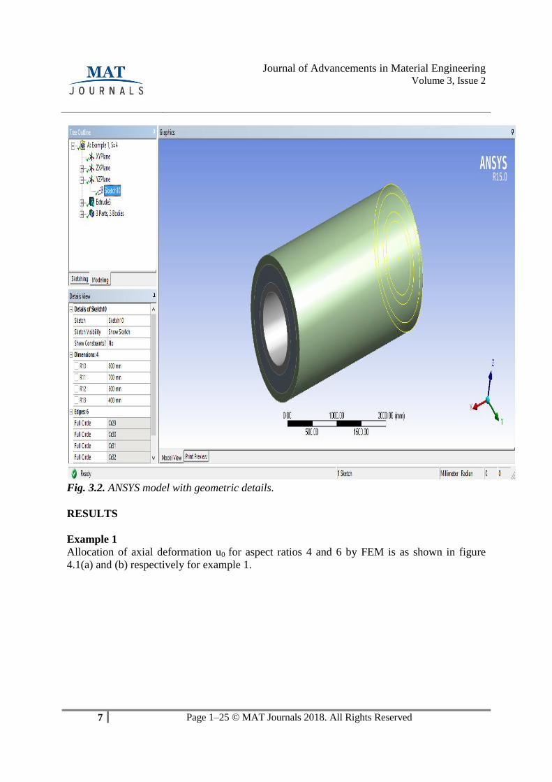
Fig. 3.2. ANSYS model with geometric details.

RESULTS

Example 1

Allocation of axial deformation u0 for aspect ratios 4 and 6 by FEM is as shown in figure

4.1(a) and (b) respectively for example 1.



4.1(a)

4.1(b)

Fig. 4.1. Axial deformation u0 for aspect ratios 4 and 6 by FEM for example 1.



Table 4.1. Axial deformation (u0) of composite beam for aspect ratios S=4 and S=6.

Source Method At S=4 S=6

ANSYS work-

bench

FEM x=0 1.2179E-5 1.2284E-5

x=0.5L 0 0

x=L 1.2179E-5 1.2284E-5

Variation of axial deformation (u0) of

composite beam subjected to uniform

downward pressure with FEM is tabula-

rized in table 4.1.

FEM results are plotted by keeping axial

deformation (u0) for aspect ratios 4 and 6

on Y-axis and length of the beam on X-

axis as in graphs of figure 4.2 (a) and (b)

respectively for example 1.

4.2(a)

4.2(b)

Fig. 4.2. Variation of axial deformation (u0) with length for aspect ratios 4 and 6 for example

1.

Allocation of transverse deformation (w0)

for aspect ratios 4 and 6 by FEM is as

shown in figure 4.3(a) and (b) respectively

for example 1.



4.3(a)

4.3(b)

Fig. 4.3. Transverse deformation (w0) for aspect ratios 4 and 6 by FEM for example 1.

Table 4.2. Transverse deformation (w0) of composite beam for aspect ratios S=4 and S=6.


ANSYS work-

bench

FEM x=0 0.00012372 0.00012374

x=0.5L 1.542E-7 8.315E-8

x=L 0.00012403 0.0001239

Variation of transverse deformation (w0) of composite beam subjected to uniform downward

pressure with FEM is tabularized in table 4.2.



FEM results are plotted by keeping transverse deformation (w0) for aspect ratios 4 and 6 on

Y-axis and length of the beam on X-axis as in graphs of figure 4.4(a) and (b) respectively for

example 1.

4.4(a)

4.4(b)

Fig. 4.4. Variation of transverse deformation (w0) with length for aspect ratios 4 and 6 for

example 1.

Allocation of normal stress (σx) for aspect ratios 4 and 6 by FEM is as shown in figure 4.5(a)

and (b) respectively for example 1.



4.5(a)

4.5(b)

Fig. 4.5. Distribution of normal stress (σx) for aspect ratios 4 and 6 by FEM.

Table 4.3. Normal stress (σx) of composite beam for aspect ratios S=4 and S=6.


ANSYS work-

bench

FEM x=0 0.021498 0.012219

x=0.5L 0.00467 2.2785E-5

x=L 0.012143 0.012265



Variation of normal stress (σx) of composite beam subjected to uniform downward pressure

with FEM is tabularized in table 4.3.

Distribution by FEM results are plotted by keeping normal stress (σx) for aspect ratios 4 and 6

on Y-axis and length of the beam on X-axis as in graphs of figure 4.6(a) and (b) respectively

for example 1.

4.6(a)

4.6(b)

Fig. 4.6. Variation of normal stress (σx) with length for aspect ratios 4 and 6 for example 1.

Allocation of shear stress (τxy) for aspect ratios 4 and 6 by FEM is as shown in figure 4.7(a)




4.7(a)

4.7(b)

Fig. 4.7. Distribution of shear stress (τxy) for aspect ratios 4 and 6 by FEM for example 1.

Table 4.4. Shear stress (τxy) of composite beam for aspect ratios S=4 and S=6.


ANSYS work-

bench

FEM x=0 0.0023153 0.0022734

x=0.5L 0 0

x=L 0.0023153 0.0022734



Variation of shear stress (τxy) of composite beam subjected to uniform downward pressure

with FEM is tabularized in table 4.4.

Distribution by FEM results are plotted by keeping transverse deformation (τxy) for aspect

ratios 4 and 6 on Y-axis and length of the beam on X-axis as in graphs of figure 4.8(a) and

(b) respectively for example 1.

4.8(a)

4.8(b)

Fig. 4.8. Variation of shear stress (τxy) with length for aspect ratios 4 and 6 for example 1.

Example 2

Allocation of axial deformation u0 for aspect ratios 4 and 6 by FEM is as shown in figure




4.9(a)

4.9(b)

Fig. 4.9. Axial deformation u0 for aspect ratios 4 and 6 by FEM for example 2.

Table 4.5. Axial deformation (u0) of composite beam for aspect ratios S=4 and S=6.


ANSYS work-

bench

FEM x=0 1.1046E-5 1.156E-5

x=0.5L 0 1.6544E-21

x=L 1.1046E-5 1.156E-5



Variation of axial deformation (u0) composite beam subjected to uniform downward pressure

with FEM is tabularized in table 4.5.for example 2.

FEM results are plotted by keeping axial deformation (u0) for aspect ratios 4 and 6 on Y-axis

and length of the beam on X-axis as in graphs of figure 4.10 (a) and (b) respectively for ex-

ample 2.

4.10(a)

4.10(b)

Fig. 4.10. Variation of axial deformation (u0) with length for aspect ratios 4 and 6 for exam-

ple 2.

Allocation of transverse deformation (w0) for aspect ratios 4 and 6 by FEM is as shown in

figure 4.11(a) and (b) respectively for example 2.



4.11(a)

4.11(b)

Fig. 4.11. Transverse deformation (w0) for aspect ratios 4 and 6 by FEM for example 2.

Table 4.6. Transverse deformation (w0) of composite beam for aspect ratios S=4 and S=6.


ANSYS work-

bench

FEM x=0 9.5564E-5 0.0001054

x=0.5L 1.2566E-7 1.6623E-7

x=L 9.58E-5 0.0001057



Variation of transverse deformation (w0) of composite beam subjected to uniform downward

pressure with FEM is tabularized in table 4.6.for example 2.

FEM results are plotted by keeping transverse deformation (w0) for aspect ratios 4 and 6 on

Y-axis and length of the beam on X-axis as in graphs of figure 4.12(a) and (b) respectively.

4.12(a)

4.12(b)

Fig. 4.12. Variation of transverse deformation (w0) with length for aspect ratios 4 and 6 for

example 2.

Allocation of normal stress (σx) for aspect ratios 4 and 6 by FEM is as shown in figure




4.13(a)

4.13(b)

Fig. 4.13. Distribution of normal stress (σx) for aspect ratios 4 and 6 by FEM for example 2.

Table 4.7. Normal stress (σx) of composite beam for aspect ratios S=4 and S=6.


ANSYS work-

bench

FEM x=0 0.018652 0.011176

x=0.5L 0.0048 0.0008

x=L 0.00910 0.00948



Variation of normal stress (σx) of composite beam subjected to uniform downward pressure

with FEM is tabularized in table 4.7 for example 2.

Distribution by FEM results are plotted by keeping transverse deformation (σx) for aspect ra-

tios 4 and 6 on Y-axis and length of the beam on X-axis as in graphs of figure 4.14(a) and (b)

respectively for example 2.

4.14(a)

4.14(b)

Fig. 4.14. Variation of normal stress (σx) with length for aspect ratios 4 and 6 for example 2.

Allocation of shear stress (τxy) for aspect ratios 4 and 6 by FEM is as shown in figure 4.15(a)




4.15(a)

4.15(b)

Fig. 4.15. Distribution of shear stress (τxy) for aspect ratios 4 and 6 by FEM for example 2.

Table 4.8. Shear stress (τxy) of composite beam for aspect ratios S=4 and S=6.


ANSYS work-

bench

FEM x=0 0.0020575 0.0021222

x=0.5L 5.8208E-11 0

x=L 0.0020575 0.0021222



Variation of shear stress (τxy) of composite beam subjected to uniform downward pressure

with FEM is tabularized in table 4.8 for example 2.

Distribution by FEM results are plotted by keeping transverse deformation (τxy) for aspect

ratios 4 and 6 on Y-axis and length of the beam on X-axis as in graphs of figure 4.16(a) and

(b) respectively for example 2.

4.16(a)

4.16(b)

Fig. 4.16. Variation of shear stress (τxy) with length for aspect ratios 4 and 6 for example 2.

DISCUSSIONS

Results acquired by FEM for two compo-

site beams with different layering pattern

of composite material for two different

aspect ratios S=4 and S=6.

1. Axial deformation (u0):

For aspect ratio S=4 as seen from

table 4.1 and 4.5 for example 2

value at x=0 is greater than value

for example 1 by 1.13E-06, at

x=0.5L there is no difference in

values and at x=L value for exam-

ple 2 is less than value for example

1 by 1.13E-06.





x=0.5L value is greater than value

for example 1 by 1.65E-21 and at

x=L value for example 2 is less



than value for example 1 by 7.24E-

07.

2. Transverse deformation (w0):





x=0.5L value is less than value for

example 1 by 2.85E-08 and at x=L

value for example 2 is less than

value for example 1 by 2.82E-05.





x=0.5L value is greater than value

for example 1 by 8.31E-08 and at

x=L value for example 2 is less

than value for example 1 by 1.82E-

05.

3. Normal stress (σx):

















4. Shear stress (τxy):













x=0.5L there is no difference in

values and at x=L value for exam-

ple 2 is less than value for example

1 by 1.51E-04.

REFERENCES

1. Meena, V. and A. Saroya. Study of

Mechanical Properties of Hybrid Nat-

ural Fiber Composite, 2011.

2. Wang, C., et al. Shear deformable

beams and plates: Relationships with

classical solutions, Elsevier, 2000.

3. Courtney, T. H., Mechanical behavior

of materials, Waveland Press, 2005.

4. Hull, D. and T. Clyne, An introduc-

tion to composite materials, Cam-

bridge university press, 1996.

5. Lord Rayleigh, J. The theory of

sound, vol. 1, New York, NY: Dover

Publications, 1945.

6. Timoshenko, S. P. "LXVI. On the

correction for shear of the differential

equation for transverse vibrations of

prismatic bars." The London, Edin-

burgh, and Dublin Philosophical

Magazine and Journal of Science,

1921. 41(245): 744–746.

7. Ghugal, Y. and R. Shimpi, "A review

of refined shear deformation theories

for isotropic and anisotropic lami-

nated beams." Journal of reinforced

plastics and composites, 2001. 20(3):

255–272.

8. Cowper, G. The shear coefficient in

Timoshenko's beam theory, ASME,

1966.



9. Reddy, J. N., Mechanics of laminated

composite plates and shells: theory

and analysis, CRC press, 2004.

10. Rehfield, L. W. and P. Murthy, "To-

ward a new engineering theory of

bending- Fundamentals." AIAA jour-

nal, 1982. 20(5): 693–699.

11. Bickford, W., "A consistent higher

order beam theory." Developments in

Theoretical and Applied Mechanics,

1982. 11: 137–150.

12. MURTY, K., "Toward a consistent

beam theory." AIAA journal, 1984.

22(6): 811–816.

13. Levinson, M., "A new rectangular

beam theory." Journal of Sound and

vibration, 1981. 74(1): 81–87.

14. Bhimaraddi, A. and K. Chandrashek-

hara, "Observations on higher-order

beam theory." Journal of Aerospace

Engineering, 1993. 6(4): 408–413.

15. Baluch, M. H., et al., "Technical

theory of beams with normal strain."

Journal of Engineering Mechanics,

1984. 110(8): 1233–1237.

16. Irretier, H., Refined effects in beam

theories and their influence on the

natural frequencies of beams. Refined

dynamical theories of beams, plates

and shells and their applications,

1987. Springer: 163–179.

17. Kant, T. and A. Gupta, "A finite ele-

ment model for a higher-order shear-

deformable beam theory." Journal of

Sound and vibration, 1988. 125(2):

193–202.

18. Heyliger, P. and J. Reddy, "A higher

order beam finite element for bending

and vibration problems." Journal of

Sound and vibration, 1988. 126(2):

309–326.

19. Averill, R. and J. Reddy, "An assess-

ment of four‐ noded plate finite ele-

ments based on a generalized

third‐ order theory." International

journal for numerical methods in en-

gineering, 1992. 33(8): 1553–1572.

20. Reddy, J. N., An introduction to the

finite element method, McGraw-Hill

New York, 1993.

21. Stein, M., "Vibration of beams and

plate strips with three-dimensional

flexibility." Journal of applied me-

chanics, 1989. 56(1): 228–231.

22. Vlasov, V. Z., "Beams, plates and

shells on elastic foundations." Israel

Program for Scientific Translations,

1966.

Documents

Analysis and Comparison of Two Composite Beams by Finite