Bayesian reconstruction of past land-cover from pollen data: model

robustness and sensitivity to auxiliary variables

Behnaz Pirzamanbein ∗1,2,3, Johan Lindstrom1 and Anneli Poska4,5

1Department of Applied Mathematics and Computer Science, Technical University of Denmark

2Centre for Mathematical Sciences, Lund University, Sweden

3Centre for Environmental and Climate Research, Lund University, Sweden

4Department of Physical Geography and Ecosystems Analysis, Lund University, Sweden

5Institute of Geology, Tallinn University of Technology, Estonia

Abstract

Realistic depictions of past land cover are needed to investigate prehistoric environmental changes,

effects of anthropogenic deforestation, and long term land cover-climate feedbacks. Observation

based reconstructions of past land cover are rare and commonly used model based reconstructions

exhibit considerable differences. Recently Pirzamanbein et al. (Spatial Statistics, 24:14–31, 2018)

developed a statistical interpolation method that produces spatially complete reconstructions of past

land cover from pollen assemblage. These reconstructions incorporate a number of auxiliary datasets

raising questions regarding the method’s sensitivity to different auxiliary datasets.

Here the sensitivity of the method is examined by performing spatial reconstructions for northern

Europe during three time periods (1900 CE, 1725 CE and 4000 BCE). The auxiliary datasets

considered include the most commonly utilized sources of past land-cover data — e.g. estimates

produced by a dynamic vegetation (DVM) and anthropogenic land-cover change (ALCC) models.

Five different auxiliary datasets were considered, including different climate data driving the DVM

and different ALCC models. The resulting reconstructions were also evaluated using cross-validation

for all the time periods. For the recent time period, 1900 CE, the different land-cover reconstructions

were compared against a present day forest map.

The validation confirms that the statistical model provides a robust spatial interpolation tool

with low sensitivity to differences in auxiliary data and high capacity to capture information in the

pollen based proxy data. Further auxiliary data with high spatial detail improves model performance

for areas with complex topography or few observations.

∗Corresponding author: Behnaz Pirzamanbein, bepi@dtu.dk

1

arX

iv:1

703.

0671

9v2

[st

at.A

P] 3

Nov

201

8

1 Introduction

The importance of terrestrial land cover for the global carbon cycle and its impact on the climate

system is well recognized (e.g. Claussen et al., 2001; Brovkin et al., 2006; Arneth et al., 2010; Christidis

et al., 2013). Many studies have found large climatic effects associated with changes in land cover.

Forecast simulations evaluating the effects of human induced global warming predict a considerable

amplification of future climate change, especially for Arctic areas (Zhang et al., 2013; Richter-Menge

et al., 2011; Chapman and Walsh, 2007; Koenigk et al., 2013; Miller and Smith, 2012). The past

anthropogenic deforestation of the temperate zone in Europe was lately demonstrated to have an

impact on regional climate similar in amplitude to present day climate change (Strandberg et al., 2014).

However, studies on the effects of vegetation and land-use changes on past climate and carbon cycle

often report considerable differences and uncertainties in their model predictions (de Noblet-Ducoudre

et al., 2012; Olofsson, 2013).

One of the reasons for such widely diverging results could be the differences in past land-cover

descriptions used by climate modellers. Possible land-cover descriptions range from static present-day

land cover (Strandberg et al., 2011), over simulated potential natural land cover from dynamic (or

static) vegetation models (DVMs) (e.g. Brovkin et al., 2002; Hickler et al., 2012), to past land-cover

scenarios combining DVM derived potential vegetation with estimates of anthropogenic land-cover

change (ALCC) (Strandberg et al., 2014; Pongratz et al., 2008; de Noblet-Ducoudre et al., 2012).

Differences in input climates, mechanistic and parametrisation differences of DVMs (Prentice et al.,

2007; Scheiter et al., 2013), and significant variation between existing ALCC scenarios (e.g. Kaplan

et al., 2009; Pongratz et al., 2008; Goldewijk et al., 2011; Gaillard et al., 2010) further contribute

to the differences in past land-cover descriptions. These differences can lead to largely diverging

estimates of past land-cover dynamics even when the most advanced models are used (Strandberg et al.,

2014; Pitman et al., 2009). Thus, reliable land-cover representations are important when studying

biogeophysical impacts of anthropogenic land-cover change on climate.

The palaeoecological proxy based land-cover reconstructions recently published by Pirzamanbein

et al. (2014, 2018) were designed to overcome the problems described above. And to provide a proxy

based land-cover description applicable for a range of studies on past vegetation and its interactions

with climate, soil and humans. These reconstructions use the pollen based land-cover composition

(PbLCC) published by Trondman et al. (2015) as a source of information on past land-cover composition.

The PbLCC are point estimates, depicting the land-cover composition of the area surrounding each

of the studied sites. Spatial interpolation is needed to fill the gaps between observations and to

2

produce continuous land-cover reconstructions. Conventional interpolation methods might struggle

when handling noisy, spatially heterogeneous data (Heuvelink et al., 1989; de Knegt et al., 2010), but

statistical methods for spatially structured data exist (Gelfand et al., 2010; Blangiardo and Cameletti,

2015).

In Pirzamanbein et al. (2018) a statistical model based on Gaussian Markov Random Fields (Lindgren

et al., 2011; Rue and Held, 2005) was developed to provide a reliable, computationally effective and

freeware based spatial interpolation technique. The resulting statistical model combines PbLCC data

with auxiliary datasets; e.g. DVM output, ALCC scenarios, and elevation; to produce reconstructions

of past land cover. The auxiliary data is subject to the differences and uncertainties outlined above and

the choice of auxiliary data could influence the accuracy of the statistical model. The major objectives

of this paper are: 1) To draw attention of climate modelling community to a novel set of spatially

explicit pollen-proxy based land-cover reconstructions suitable for climate modelling; 2) to present and

test the robustness of the spatial interpolation model developed by Pirzamanbein et al. (2018); and 3)

to evaluate the models capacity to recover information provided by PbLCC proxy data and to analyse

its sensitivity to different auxiliary datasets.

2 Material and Methods

The studied area covers temperate, boreal and alpine-arctic biomes of central and northern Europe

(45◦N to 71◦N and 10◦W to 30◦E). The PbLCC data published in Trondman et al. (2015) consists of

proportions of coniferous forest, broadleaved forest and unforested land presented as gridded (1◦ × 1◦)

data points placed irregularly across northern-central Europe. Altogether 175 grid cells containing proxy

data were available for 1900 CE, 181 for 1725 CE, and 196 for the 4000 BCE time-period (Figure 1,

column 2).

Four different model derived datasets, depicting past land cover, along with elevation were considered

as potential auxiliary datasets. In each case potential natural vegetation composition estimated by the

DVM LPJ-GUESS (Lund-Potsdam-Jena General Ecosystem Simulator; Smith et al., 2001; Sitch et al.,

2003) were combined with an ALCC scenario to adjust for human land use (see Pirzamanbein et al.,

2014, for details):

K-LRCA3: Combines the ALCC scenario KK10 (Kaplan et al., 2009) and the potential natural

vegetation from LPJ-GUESS. Climate forcing for the DVM was derived from RCA3 (Rossby

Centre Regional Climate Model, Samuelsson et al., 2011) at annual time and 0.44◦× 0.44◦ spatial

resolution (Figure 1, column 3),

3

K-LESM: Combines the ALCC scenario KK10 and the potential natural vegetation from LPJ-GUESS.

Climate forcing for the DVM was derived from the Earth System Model (ESM; Mikolajewicz

et al., 2007) at centennial time and 5.6◦ × 5.6◦ spatial resolution. To interpolate data into annual

time and 0.5◦ × 0.5◦ spatial resolution climate data from 1901–1930 CE provided by the Climate

Research Unit was used (Figure 1, column 4),

H-LRCA3: Combines the ALCC scenario from the History Database of the Global Environment (HYDE;

Goldewijk et al., 2011) and vegetation from LPJ-GUESS with RCA3 climate forcing (Figure 1,

column 5),

H-LESM: Combines the ALCC scenario from HYDE and vegetation from LPJ-GUESS with ESM

climate forcing (Figure 1, column 6).

The elevation data (denoted SRTMelev) was obtained from the Shuttle Radar Topography Mission

(Becker et al., 2009) (Figure 1, column 1 row 2).

Finally, a modern forest map based on data from the European Forest Institute (EFI) is used for

evaluation of the model’s performance for the 1900 CE time period. The EFI forest map (EFI-FM)

is based on a combination of satellite data and national forest-inventory statistics from 1990–2005

(Pivinen et al., 2001; Schuck et al., 2002) (Figure 1, column 1 row 1). All auxiliary data were up-scaled

to 1◦ × 1◦ spatial resolution, matching the pollen based reconstructions, before usage as model input.

2.1 Statistical Model for Land-cover Compositions

A Bayesian hierarchical model is used to interpolate the PbLCC data; here we only provide a brief

overview of the model, mathematical and technical details can be found in Pirzamanbein et al. (2018).

The model can be seen as a special case of a generalized linear mixed model with a spatially correlated

random effect. An alternative interpretation of the model is as an empirical forward model (direction

of arrows in Figure 2) where parameters affect the latent variables which in turn affect the data.

Reconstructions are obtained by inverting the model (i.e. computing the posterior) to obtain the latent

variables given the data.

The PbLLC derived proportions of land cover (coniferous forest, broadleaved forest and unforested

land), denoted Y PbLCC, are seen as draws from a Dirichlet distribution (Kotz et al., 2000, Ch. 49)

given a vector of proportions, Z, and a concentration parameter, α (controlling the uncertainty:

V(Y PbLCC) ∝ 1/α). Since the proportions have to obey certain restrictions (0 ≤ Zk ≤ 1 and∑3k=1 Zk = 1, were k indexes the land-cover types), a link function is used to transform between the

4

Figure 1: Data used in the modelling. The first column shows (from top to bottom) the EFI-FM,SRTMelev, and the colorkey for the land-cover compositions, coniferous forest (CF), broadleaved forest(BF) and unforested land (UF). The remaining columns give (from left to right) the PbLCC (Trondmanet al., 2015) and the four model based compositions considered as potential covariates: K-LRCA3,K-LESM, H-LRCA3, and H-LESM. Here K/H indicates KK10 (Kaplan et al., 2009) or HYDE (Goldewijket al., 2011) land use scenarios and LRCA3/LESM indicates the climate — Rossby Centre RegionalClimate Model (Samuelsson et al., 2011) or Earth System Model (Mikolajewicz et al., 2007) — used todrive the vegetation model. The three rows represent (from top to bottom) the time periods 1900 CE,1725 CE, and 4000 BCE.

Y PbLCCData model

ZLCRs = f (η)ZLCRs = f (η)

Parameters

Latent variablesη µ X= +

αβ

BCovariates

κ Σ

Figure 2: Hierarchical graph describing the conditional dependencies between observations (whiterectangle) and parameters (grey rounded rectangles) to be estimated. The white rounded rectanglesare computed based on the estimations. In a generalized linear mixed model framework, η is the linearpredictor — consisting of a regression term, µ, and a spatial random effect, X. The link function, f(η),transforms between linear predictor and proportions, which are matched to the observed land coverproportions, Y PbLCC, using a Dirichlet distribution.

5

Table 1: Six different models and corresponding covariates. SRTMelev is elevation (Becker et al., 2009),K/H indicates KK10 (Kaplan et al., 2009) or HYDE (Goldewijk et al., 2011) land use scenarios andLRCA3/LESM indicates vegetation model driven by climate from the Rossby Centre Regional ClimateModel (Samuelsson et al., 2011) or from an Earth System Model (Mikolajewicz et al., 2007).

ModelCovariates

Intercept SRTMelev K-LESM K-LRCA3 H-LESM H-LRCA3

Constant xElevation x xK-LESM x x xK-LRCA3 x x xH-LESM x x xH-LRCA3 x x x

proportions and the linear predictor, η:

Zk = f(η) =

eηk

1+∑2i=1 e

ηifor k = 1, 2

11+

∑2i=1 e

ηifor k = 3

ηk = f−1(Z) = log

(Zk

Z3

)for k = 1, 2

Here f−1(Z) is the additive log-ratio transformation (Aitchison, 1986), a multivariate extension of the

logit transformation.

The linear predictor consists of a mean structure and a spatially dependent random effect, η = µ+X.

The mean structure is modelled as a linear regression, µ = Bβ; i.e. a combination of covariates, B,

and regression coefficients, β. To aid in variable selection and suppress uninformative covariates a

horseshoe prior (Park and Casella, 2008; Makalic and Schmidt, 2016) is used for β. The main focus of

this paper is to evaluate the model sensitivity to the choice of covariates (i.e. the auxiliary datasets).

The PbLCC is modelled based on six different sets of covariates: 1) Intercept, 2) SRTMelev, 3) K-LESM,

4) K-LRCA3, 5) H-LESM, and 6) H-LRCA3; illustrated in Figure 1. A summary of the different models is

given in Table 1.

Finally, the spatially dependent random effect is modelled using a Gaussian Markov Random Field

(Lindgren et al., 2011) with two parameters: κ, controlling the strength of the spatial dependence and

Σ, controlling the variation within and between the fields (i.e. the correlation among different land

cover types).

Model estimation and reconstructions are performed using Markov Chain Monte Carlo (Brooks

et al., 2011) with 100 000 samples and a burn-in of 10 000 (See Pirzamanbein et al., 2018, for details.).

Output from the Markov Chain Monte Carlo are then used to compute land-cover reconstructions

6

(as posterior expectations, E(Z|Y PbLCC)) and uncertainties in the form of predictive regions. The

predictive regions describe the uncertainties associated with the reconstructions; including uncertainties

in model parameters and linear predictor.

2.2 Testing the Model Performance

To evaluate model performance, we compared the land-cover reconstructions from different models for

the 1900 CE time period with the EFI-FM by computing the average compositional distances (Aitchison

et al., 2000; Pirzamanbein et al., 2018). This measure is similar to root mean square error in R2 but it

accounts for compositional properties (i.e. 0 ≤ Zk ≤ 1 and∑3

k=1 Zk = 1).

Since no independent observational data exists for the 1725 CE and 4000 BCE time periods, we

applied a 6-fold cross-validation scheme (Hastie et al., 2001, Ch. 7.10) to all models and time periods.

The cross-validation divides the observations into 6 random groups and the reconstruction errors for

each group when using only observations from the other 5 groups are computed. To further compare

predictive performance of the models Deviance Information Criteria (DIC; see Ch. 7.2 in Gelman

et al., 2014) were computed for all models and time periods. The DIC is a hierarchical modelling

generalization of the Akaike and Bayesian information criteria (Hastie et al., 2001, Ch. 7).

3 Results and Discussion

Fossil pollen is a well-recognized information source of vegetation dynamics and generally accepted as

the best observational data on past land-cover composition and environmental conditions (Trondman

et al., 2015).

Today, central and northern Europe have, at the subcontinental spatial scale, the highest density

of palynologically investigated sites on Earth. However, even there the existing pollen records are

irregularly placed, leaving some areas with scarce data coverage (Fyfe et al., 2015). The collection of

new pollen data to fill these gaps is very time consuming and cannot be performed everywhere. All this

makes pollen data, in their original format, heavily underused, since the data is unsuitable for models

requiring continuous land-cover representations as input. The lack of spatially explicit proxy based

land cover data directly usable in climate models has been hampering the correct representation of past

climate-land cover relationship.

Regrettably, the commonly used DVM derived representations of past land cover exhibit large

variation in vegetation composition estimates. The model derived land-cover datasets used as auxiliary

data (Table 1) show large variation in estimated extents of coniferous and broadleaved forests, and

7

unforested areas for all of the studied time periods (Figure 1). These substantial differences illustrate

large deviances between model based estimates of the past land-cover composition due to differences in

applied climate forcing and/or ALCC scenarios. Differences in climate model outputs (Harrison et al.,

2014; Gladstone et al., 2005) and ALCC model estimates (Gaillard et al., 2010) have been recognized

in earlier comparison studies and syntheses. The effect of the differences in input climate forcing and

ALCC scenario on DVM estimated land-cover composition presented here are especially pronounced

for central and western Europe, and for elevated areas in northern Scandinavia and the Alps (Figure

1). In general the KK10 ALCC scenario produces larger unforested areas, notably in western Europe,

compared to the HYDE scenario. Compared to the ESM climate forcing; the RCA3 forcing results

in higher proportions of coniferous forest, especially for central, northern and eastern Europe. The

described differences are clearly recognizable for all the considered time periods and are generally larger

between time periods than within each time period. The purpose of the statistical model presented

in Section 2.1 is to combine the observed PbLCC with the spatial structure in the auxiliary data to

produce data driven spatially complete maps of past land-cover that can be used directly (as input) in

others models.

To illustrate the structure of the statistical model, step by step advancement from auxiliary data

(model derived land cover) to final statistical estimates of land cover compositions for 1725 CE are

given in Figures 3 and 4. The large differences in K-LRCA3 and K-LESM are reduced by scaling with

the regression coefficients, β, capturing the empirical relationship between covariates and PbLCC

data. Thereafter, the land-cover estimates are subjected to similar adjustments due to intercept and

SRTMelev, and finally similar spatial dependent effects.

The impact of different auxiliary datasets was assessed by using the statistical model to create a

set of proxy based reconstructions of past land cover for central and northern Europe during three

time periods (1900 CE, 1725 CE and 4000 BCE; see Figures 5 and 6). Each of these reconstructions

were based on the irregularly distributed observed pollen data (PbLCC), available for ca 25% of the

area, together with one of the six models (Table 1) using different combinations of the auxiliary data

(Figure 1).

The resulting land-cover reconstructions exhibit considerably higher similarity with the PbLCC

data than any of the auxiliary land-cover datasets for all tested models and time periods (Figures 5

and 6). At first the similarity among the reconstructions might seem contradictory, but recall that

the model allows for, and estimates, different weighting (the regression coefficients, β:s) for each of

the auxiliary datasets. Thus, the resulting reconstructions do not rely on the absolute values in the

auxiliary datasets, only their spatial patterns. As a result, model performance for elevated areas and

8

20

40

60

80

20 40 60 80

20

40

60

CF

BF

UF

80 20

40

60

80

20 40 60 80

20

40

60

CF

BF

UF

80

PbLCC K-LESM K-LRCA3

Figure 3: Advancement of the model for two locations at 1725 CE. Starting from the value of theK-LRCA3 and K-LESM covariates (∗), the cumulative effects of regression coefficients, β, (+); theintercept and SRTMelev covariates (•); and, finally, the spatial dependency structures (◦), are illustrated.With the final points (◦) corresponding to the land-cover reconstructions and � marking the observedpollen based land-cover composition.

Figure 4: Advancement of K-LESM models for the 1725 CE time period: (a) shows the effect of interceptand SRTMelev, (b) shows the mean structure, µ, including all the covariates, (c) shows the spatialdependency structure and finally (d) shows the resulting land-cover reconstructions obtained by adding(b) and (c).

9

Figure 5: Land-cover reconstructions using PbLCC for the 1900 CE time periods (top row). Thereconstructions are based on six different models (see Table 1) with different auxiliary datasets. Locationsand compositional values of the available PbLCC data are given by the black rectangles. Middle rowshows the compositional distances between each model and the Constant model. Bottom row showsthe compositional distances between each model and the EFI-FM.

10

Figure 6: Land-cover reconstructions using local estimates of PbLCC for the 1725 CE (top) and 4000BCE (bottom) time periods. The reconstructions are based on six different models (see Table 1) withdifferent auxiliary datasets. Locations and compositional values of the available PbLCC data are givenby the black rectangles. Third and fourth row show the compositional distances between each modeland the Constant model.

11

for the areas with low observational data coverage (e.g. eastern and south-eastern Europe) is improved

by including covariates that exhibit distinct spatial structures for the given areas (Figures 5 and 6).

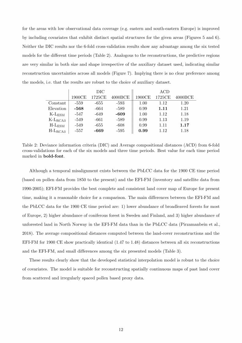
Neither the DIC results nor the 6-fold cross-validation results show any advantage among the six tested

models for the different time periods (Table 2). Analogous to the reconstructions, the predictive regions

are very similar in both size and shape irrespective of the auxiliary dataset used, indicating similar

reconstruction uncertainties across all models (Figure 7). Implying there is no clear preference among

the models, i.e. that the results are robust to the choice of auxiliary dataset.

DIC ACD1900CE 1725CE 4000BCE 1900CE 1725CE 4000BCE

Constant -559 -655 -593 1.00 1.12 1.20Elevation -568 -664 -589 0.99 1.11 1.21K-LESM -547 -649 -609 1.00 1.12 1.18K-LRCA3 -549 -661 -589 0.99 1.13 1.19H-LESM -549 -655 -608 0.99 1.11 1.17H-LRCA3 -557 -669 -595 0.99 1.12 1.18

Table 2: Deviance information criteria (DIC) and Average compositional distances (ACD) from 6-foldcross-validations for each of the six models and three time periods. Best value for each time periodmarked in bold-font.

Although a temporal misalignment exists between the PbLCC data for the 1900 CE time period

(based on pollen data from 1850 to the present) and the EFI-FM (inventory and satellite data from

1990-2005); EFI-FM provides the best complete and consistent land cover map of Europe for present

time, making it a reasonable choice for a comparison. The main differences between the EFI-FM and

the PbLCC data for the 1900 CE time period are: 1) lower abundance of broadleaved forests for most

of Europe, 2) higher abundance of coniferous forest in Sweden and Finland, and 3) higher abundance of

unforested land in North Norway in the EFI-FM data than in the PbLCC data (Pirzamanbein et al.,

2018). The average compositional distances computed between the land-cover reconstructions and the

EFI-FM for 1900 CE show practically identical (1.47 to 1.48) distances between all six reconstructions

and the EFI-FM, and small differences among the six presented models (Table 3).

These results clearly show that the developed statistical interpolation model is robust to the choice

of covariates. The model is suitable for reconstructing spatially continuous maps of past land cover

from scattered and irregularly spaced pollen based proxy data.

12

0

20

40

60

80

0 20 40 60 80

0

20

40

60

80

C

B

U

Ratio of ellipses:Intercept = 60%Elevation = 58%K-L RCA3 = 60%

K-L ESM = 61%

H-L RCA3 = 59%

H-L ESM = 60%

1900

CE

Obs. (PbLCC)EFI-FM Intercept Elevation K-LRCA3 H-LRCA3 H-LESM

0

20

40

60

80

0 20 40 60 80

0

20

40

60

80

C

B

U

Ratio of ellipses:Intercept = 56%Elevation = 52%K-L RCA3 = 60%

K-L ESM = 61%

H-L RCA3 = 60%

H-L ESM = 59% 0

20

40

60

80

0 20 40 60 80

0

20

40

60

80

C

B

U

Ratio of ellipses:Intercept = 60%Elevation = 59%K-L RCA3 = 58%

K-L ESM = 59%

H-L RCA3 = 56%

H-L ESM = 63%

0

20

40

60

80

0 20 40 60 80

0

20

40

60

80

C

B

U

Ratio of ellipses:Intercept = 60%Elevation = 59%K-L RCA3 = 58%

K-L ESM = 61%

H-L RCA3 = 59%

H-L ESM = 61%

1725

CE

0

20

40

60

80

0 20 40 60 80

0

20

40

60

80

C

B

U

Ratio of ellipses:Intercept = 60%Elevation = 59%K-L RCA3 = 60%

K-L ESM = 60%

H-L RCA3 = 59%

H-L ESM = 60% 0

20

40

60

80

0 20 40 60 80

0

20

40

60

80

C

B

U

Ratio of ellipses:Intercept = 61%Elevation = 61%K-L RCA3 = 60%

K-L ESM = 66%

H-L RCA3 = 59%

H-L ESM = 64%

0

20

40

60

80

0 20 40 60 80

0

20

40

60

80

C

B

U

Ratio of ellipses:Intercept = 65%Elevation = 65%K-L RCA3 = 65%

K-L ESM = 61%

H-L RCA3 = 64%

H-L ESM = 64%

4000

BC

E

0

20

40

60

80

0 20 40 60 80

0

20

40

60

80

C

B

U

Ratio of ellipses:Intercept = 71%Elevation = 71%K-L RCA3 = 72%

K-L ESM = 67%

H-L RCA3 = 71%

H-L ESM = 68% 0

20

40

60

80

0 20 40 60 80

0

20

40

60

80

C

B

U

Ratio of ellipses:Intercept = 71%Elevation = 71%K-L RCA3 = 71%

K-L ESM = 69%

H-L RCA3 = 71%

H-L ESM = 71%

K-LESM

Figure 7: The prediction regions and fraction of the ternary triangle covered by these regions arepresented for three locations, the six models, and the 1900 CE, 1725 CE and 4000 BCE time periods.

13

EFI-FM Elevation K-LESM K-LRCA3 H-LESM H-LRCA3

1900 CE

Constant 1.48 0.08 0.18 0.20 0.17 0.19Elevation 1.49 0.19 0.21 0.18 0.20K-LESM 1.48 0.09 0.07 0.09K-LRCA3 1.48 0.11 0.06H-LESM 1.48 0.08H-LRCA3 1.48

1725 CE

Constant 0.10 0.16 0.16 0.17 0.17Elevation 0.14 0.11 0.14 0.13K-LESM 0.14 0.06 0.16K-LRCA3 0.15 0.07H-LESM 0.15

4000 BCE

Constant 0.11 0.21 0.17 0.22 0.19Elevation 0.19 0.12 0.20 0.15K-LESM 0.19 0.07 0.21K-LRCA3 0.18 0.07H-LESM 0.20

Table 3: The average compositional distances among the six models fitted to the data for each of thethree time periods.

4 Conclusions

The statistical model and Bayesian interpolation method presented here has been specially designed

for handling irregularly spaced palaeo-proxy records like pollen data and, dependent on proxy data

availability, is globally applicable. The model produces land-cover maps by combining irregularly

distributed pollen based estimates of land cover with auxiliary data and a statistical model for spatial

structure. The resulting maps capture important features in the pollen proxy data and are reasonably

insensitive to the use of different auxiliary datasets.

Auxiliary datasets considered were complied from commonly utilized sources of past land-cover data

(outputs from a dynamic vegetation model using different climatic drivers and anthropogenic land-cover

changes scenarios). These datasets exhibit considerable differences in their recreation of the past land

cover. Emphasizing the need for the independent, proxy based past land-cover maps created in this

paper.

Evaluation of the model’s sensitivity indicates that the proposed statistical model is robust to

the choice of auxiliary data and only considers features in the auxiliary data that are consistent with

the proxy data. However, auxiliary data with detailed spatial information considerably improves the

interpolation results for areas with low proxy data coverage, with no reduction in overall performance.

This modelling approach has demonstrated a clear capacity to produce empirically based land-

14

cover reconstructions for climate modelling purposes. Such reconstructions are necessary to evaluate

anthropogenic land-cover change scenarios currently used in climate modelling and to study past

interactions between land cover and climate with greater reliability. The model will also be very useful

for producing reconstructions of past land cover from the global pollen proxy data currently being

produced by the PAGES (Past Global changES) LandCover6k initiative1.

5 Data availability

The database containing the reconstructions of coniferous forest, broadleaved forest and unforested

land, three fractions of land cover, for the three time-periods presented in this paper, along with

reconstructions for 1425 CE and 1000 BCE using only the K-LESM are available for download from

https://github.com/BehnazP/SpatioCompo. In addition the source code is available in the same

repository under the open source GNU General Public License.

Acronyms

DVM Dynamical vegetation model.

ALCC Anthropogenic land-cover change.

PbLCC Pollen based land-cover composition.

LPJ-GUESS The Lund-Potsdam-Jena General Ecosystem Simulator, a DVM.

EFI-FM European Forest Institute forest map.

Notation

Y PbLCC Observations, as proportions.

f Link function, transforming between proportions and linear predictor.

η Linear predictor, η = µ+X.

µ Mean structure; modelled as µ = Bβ using covariates, B, and regression coefficients, β.

X Spatially dependent random effect.

α Concentrated parameter of the Dirichlet distribution (i.e. observational uncertainty)

Σ Covariance matrix that determines the variation between and within fields

κ Scale parameter controlling the range of spatial dependency

1www.pastglobalchanges.org/ini/wg/landcover6k/intro

15

Acknowledgements

The research presented in this paper is a contribution to the two Swedish strategic research areas

Biodiversity and Ecosystems in a Changing Climate (BECC), and ModElling the Regional and Global

Earth system (MERGE). The paper is also a contribution to PAGES LandCover6k. Lindstrom has

been funded by Swedish Research Council (SRC, Vetenskapsradet) grant no 2012-5983. Poska has

been funded by SRC grant no 2016-03617 and the Estonian Ministry of Education grant IUT1-8. The

authors would like to acknowledge Marie-Jose Gaillard for her efforts in providing the pollen based

land-cover proxy data and thank her for valuable comments on this manuscript.

References

J. Aitchison. The statistical analysis of compositional data. Chapman & Hall, Ltd., 1986.

J. Aitchison, C. Barcelo-Vidal, J. Martın-Fernandez, and V. Pawlowsky-Glahn. Logratio analysis and

compositional distance. Math. Geol., 32(3):271–275, 2000.

A. Arneth, S. P. Harrison, S. Zaehle, K. Tsigaridis, S. Menon, P. J. Bartlein, J. Feichter, A. Korhola,

M. Kulmala, D. O’donnell, et al. Terrestrial biogeochemical feedbacks in the climate system. Nature

Geosci., 3(8):525–532, 2010. doi: 10.1038/ngeo905.

J. J. Becker, D. T. Sandwell, W. H. F. Smith, J. Braud, B. Binder, J. Depner, D. Fabre, J. Factor,

S. Ingalls, S. H. Kim, R. Ladner, K. Marks, S. Nelson, A. Pharaoh, G. Sharman, R. Trimmer,

J. VonRosenburg, G. Wallace, and P. Weatherall. Global bathymetry and elevation data at 30 arc

seconds resolution: SRTM30 PLUS. Marine Geol., 32(4):355–371, 2009.

M. Blangiardo and M. Cameletti. Spatial and Spatio-temporal Bayesian Models with R-INLA. Wiley,

2015.

S. Brooks, A. Gelman, G. L. Jones, and X.-L. Meng. Handbook of Markov Chain Monte Carlo. CRC

Press, 2011.

V. Brovkin, J. Bendtsen, M. Claussen, A. Ganopolski, C. Kubatzki, V. Petoukhov, and A. Andreev.

Carbon cycle, vegetation, and climate dynamics in the holocene: Experiments with the CLIMBER-2

model. Glob. Biogeochem. Cycles, 16(4):1139, 2002.

V. Brovkin, M. Claussen, E. Driesschaert, T. Fichefet, D. Kicklighter, M. Loutre, H. Matthews,

N. Ramankutty, M. Schaeffer, and A. Sokolov. Biogeophysical effects of historical land cover changes

16

simulated by six Earth system models of intermediate complexity. Clim. Dyn., 26(6):587–600, 2006.

doi: 10.1007/s00382-005-0092-6.

W. L. Chapman and J. E. Walsh. Simulations of Arctic temperature and pressure by global coupled

models. J. Clim., 20(4):609–632, 2007. doi: 10.1175/JCLI4026.1.

N. Christidis, P. A. Stott, G. C. Hegerl, and R. A. Betts. The role of land use change in the recent warming

of daily extreme temperatures. Geophys. Res. Lett., 40(3):589–594, 2013. doi: 10.1002/grl.50159.

M. Claussen, V. Brovkin, and A. Ganopolski. Biogeophysical versus biogeochemical feedbacks of

large-scale land cover change. Geophys. Res. Lett., 28(6):1011–1014, 2001.

H. J. de Knegt, F. van Langevelde, M. B. Coughenour, A. K. Skidmore, W. F. de Boer, I. M. A. Heitkonig,

N. M. Knox, R. Slotow, C. van der Waal, and H. H. T. Prins. Spatial autocorrelation and the scaling

of species–environment relationships. Ecology, 91(8):2455–2465, 2010. doi: 10.1890/09-1359.1.

N. de Noblet-Ducoudre, J.-P. Boisier, A. Pitman, G. Bonan, V. Brovkin, F. Cruz, C. Delire, V. Gayler,

B. van den Hurk, P. Lawrence, M. K. van der Molen, C. Muller, C. H. Reick, B. J. Strengers, , and

A. Voldoire. Determining robust impacts of land-use-induced land cover changes on surface climate

over North America and Eurasia: results from the first set of LUCID experiments. J. Clim., 25(9):

3261–3281, 2012. doi: 10.1175/JCLI-D-11-00338.1.

R. M. Fyfe, J. Woodbridge, and N. Roberts. From forest to farmland: pollen-inferred land cover change

across Europe using the pseudobiomization approach. Glob. Change Biol., 21(3):1197–1212, 2015.

doi: 10.1111/gcb.12776.

M.-J. Gaillard, S. Sugita, F. Mazier, A.-K. Trondman, A. Brostrom, T. Hickler, J. O. Kaplan, E. Kjell-

strom, U. Kokfelt, P. Kunes, , C. Lemmen, P. Miller, J. Olofsson, A. Poska, M. Rundgren, B. Smith,

G. Strandberg, R. Fyfe, A. Nielsen, T. Alenius, L. Balakauskas, L. Barnekov, H. Birks, A. Bjune,

L. Bjorkman, T. Giesecke, K. Hjelle, L. Kalnina, M. Kangur, W. van der Knaap, T. Koff, P. Lageras,

M. Lata lowa, M. Leydet, J. Lechterbeck, M. Lindbladh, B. Odgaard, S. Peglar, U. Segerstrom,

H. von Stedingk, and H. Seppa. Holocene land-cover reconstructions for studies on land cover-climate

feedbacks. Clim. Past, 6:483–499, 2010.

A. Gelfand, P. J. Diggle, P. Guttorp, and M. Fuentes. Handbook of spatial statistics. CRC Press, 2010.

A. Gelman, J. B. Carlin, H. S. Stern, D. Dunson, A. Vehtari, and D. B. Rubin. Bayesian Data Analysis.

Chapman & Hall/CRC, third edition, 2014.

17

R. M. Gladstone, I. Ross, P. J. Valdes, A. Abe-Ouchi, P. Braconnot, S. Brewer, M. Kageyama, A. Kitoh,

A. Legrande, O. Marti, O. R., O.-B. B., P. W. R., and V. G. Mid-Holocene NAO: A PMIP2 model

intercomparison. Geophys. Res. Lett., 32(16):L16707, 2005. doi: 10.1029/2005GL023596.

K. K. Goldewijk, A. Beusen, G. Van Drecht, and M. De Vos. The HYDE 3.1 spatially explicit database

of human-induced global land-use change over the past 12,000 years. Glob. Ecol. Biogeogr., 20(1):

73–86, 2011.

S. P. Harrison, P. J. Bartlein, S. Brewer, I. C. Prentice, M. Boyd, I. Hessler, K. Holmgren, K. Izumi,

and K. Willis. Climate model benchmarking with glacial and mid-Holocene climates. Clim. Dyn., 43

(3–4):671–688, 2014. doi: 10.1007/s00382-013-1922-6.

T. Hastie, R. Tibshirani, and J. Friedman. The Elements of Statistical Learning. Springer Series in

Statistics. Springer New York Inc., New York, NY, USA, 2001.

G. B. M. Heuvelink, P. A. Burrough, and A. Stein. Propagation of errors in spatial modelling with GIS.

Int. J. Geogr. Inf. Syst., 3(4):303–322, 1989. doi: 10.1080/02693798908941518.

T. Hickler, K. Vohland, J. Feehan, P. A. Miller, B. Smith, L. Costa, T. Giesecke, S. Fronzek, T. R.

Carter, W. Cramer, I. Kuhn, and M. T. Sykes. Projecting the future distribution of European

potential natural vegetation zones with a generalized, tree species-based dynamic vegetation model.

Glob. Ecol. Biogeogr., 21(1):50–63, 2012. doi: 10.1111/j.1466-8238.2010.00613.x.

J. O. Kaplan, K. M. Krumhardt, and N. Zimmermann. The prehistoric and preindustrial deforestation

of Europe. Quat. Sci. Rev., 28(27):3016–3034, 2009.

T. Koenigk, L. Brodeau, R. G. Graversen, J. Karlsson, G. Svensson, M. Tjernstrom, U. Willen, and

K. Wyser. Arctic climate change in 21st century CMIP5 simulations with EC-Earth. Clim. Dyn., 40

(11-12):2719–2743, 2013. doi: 10.1007/s00382-012-1505-y.

S. Kotz, N. Balakrishnan, and N. L. Johnson. Continuous Multivariate Distributions. Volume 1: Models

and Applications. Wiley, 2000.

F. Lindgren, H. Rue, and J. Lindstrom. An explicit link between Gaussian fields and Gaussian Markov

random fields: the stochastic partial differential equation approach. J. R. Stat. Soc. B, 73(4):423–498,

2011. doi: 10.1111/j.1467-9868.2011.00777.x.

E. Makalic and D. F. Schmidt. A simple sampler for the horseshoe estimator. IEEE Signal Processing

Lett., 23(1):179–182, 2016. doi: 10.1109/LSP.2015.2503725.

18

U. Mikolajewicz, M. Groger, E. Maier-Reimer, G. Schurgers, M. Vizcaıno, and A. M. Winguth. Long-

term effects of anthropogenic CO2 emissions simulated with a complex earth system model. Clim.

Dyn., 28(6):599–633, 2007. doi: 10.1007/s00382-006-0204-y.

P. A. Miller and B. Smith. Modelling tundra vegetation response to recent arctic warming. Ambio, 41

(3):281–291, 2012. doi: 10.1007/s13280-012-0306-1.

J. Olofsson. The Earth: climate and anthropogenic interactions in a long time perspective. PhD thesis,

Lund University, 2013. URL http://lup.lub.lu.se/record/3732052.

T. Park and G. Casella. The bayesian lasso. J. Am. Stat. Assoc., 103(482):681–686, 2008. doi:

10.1198/016214508000000337.

B. Pirzamanbein, J. Lindstrom, A. Poska, S. Sugita, A.-K. Trondman, R. Fyfe, F. Mazier, A. Nielsen,

J. Kaplan, A. Bjune, H. Birks, T. Giesecke, M. Kangur, M. Lata lowa, L. Marquer, B. Smith, and M.-J.

Gaillard. Creating spatially continuous maps of past land cover from point estimates: A new statistical

approach applied to pollen data. Ecol. Complex., 20:127–141, 2014. doi: 10.1016/j.ecocom.2014.09.005.

B. Pirzamanbein, J. Lindstrom, A. Poska, and M.-J. Gaillard. Modelling spatial compositional

data: Reconstructions of past land cover and uncertainties. Spatial Stat., 24:14–31, 2018. doi:

10.1016/j.spasta.2018.03.005.

A. Pitman, N. de Noblet-Ducoudre, F. Cruz, E. Davin, G. Bonan, V. Brovkin, M. Claussen, C. Delire,

L. Ganzeveld, V. Gayler, B. J. J. M. van den Hurk, P. J. Lawrence, M. K. van der Molen, C. Mller,

C. H. Reick, S. I. Seneviratne, B. J. Strengers, and A. Voldoire. Uncertainties in climate responses to

past land cover change: First results from the LUCID intercomparison study. Geophys. Res. Lett., 36

(14):n/a–n/a, 2009. doi: 10.1029/2009GL039076.

R. Pivinen, M. Lehikoinen, A. Schuck, T. Hme, S. Vtinen, P. Kennedy, and S. Folving. Combining

Earth observation data and forest statistics. Technical Report 14, European Forest Institute, Joint

Research Centre-European Commission., 2001. URL https://www.efi.int/publications-bank/

combining-earth-observation-data-and-forest-statistics. ISBN: 952-9844-84-0 ISSN: 1238-

8785.

J. Pongratz, C. Reick, T. Raddatz, and M. Claussen. A reconstruction of global agricultural areas

and land cover for the last millennium. Glob. Biogeochem. Cycles, 22(3):GB3018, 2008. doi:

10.1029/2007GB003153.

19

I. C. Prentice, A. Bondeau, W. Cramer, S. P. Harrison, T. Hickler, W. Lucht, S. Sitch, B. Smith,

and M. T. Sykes. Dynamic global vegetation modeling: quantifying terrestrial ecosystem responses

to large-scale environmental change. In J. G. Canadell, D. E. Pataki, and L. F. Pitelka, editors,

Terrestrial Ecosystems in a Changing World. Global Change — The IGBP Series, pages 175–192.

Springer, 2007. doi: 10.1007/978-3-540-32730-1 15.

J. A. Richter-Menge, M. O. Jeffries, and J. E. Overland, editors. Arctic Report Card 2011. National

Oceanic and Atmospheric Administration, 2011. URL www.arctic.noaa.gov/reportcard.

H. Rue and L. Held. Gaussian Markov Random Fields; Theory and Applications, volume 104 of

Monographs on Statistics and Applied Probability. Chapman & Hall/CRC, 2005.

P. Samuelsson, C. G. Jones, U. Willen, A. Ullerstig, S. Gollvik, U. Hansson, C. Jansson, E. Kjellstrom,

G. Nikulin, and K. Wyser. The Rossby Centre regional climate model RCA3: model description and

performance. Tellus A, 63(1):4–23, 2011.

S. Scheiter, L. Langan, and S. I. Higgins. Next-generation dynamic global vegetation models: learning

from community ecology. New Phytologist, 198(3):957–969, 2013. doi: 10.1111/nph.12210.

A. Schuck, J. van Brusselen, R. Paivinen, T. Hame, P. Kennedy, and S. Folving. Compilation of

a calibrated European forest map derived from NOAA-AVHRR data. EFI Internal Report 13,

EuroForIns, 2002.

S. Sitch, B. Smith, I. C. Prentice, A. Arneth, A. Bondeau, W. Cramer, J. Kaplan, S. Levis, W. Lucht,

M. Sykes, K. Thonicke, and S. Venevsky. Evaluation of ecosystem dynamics, plant geography and

terrestrial carbon cycling in the LPJ dynamic global vegetation model. Glob. Change Biol., 9(2):

161–185, 2003.

B. Smith, I. C. Prentice, and M. T. Sykes. Representation of vegetation dynamics in the modelling of

terrestrial ecosystems: comparing two contrasting approaches within European climate space. Glob.

Ecol. Biogeogr., 10:621–637, 2001.

G. Strandberg, J. Brandefelt, E. Kjellstrom, and B. Smith. High-resolution regional simulation of last

glacial maximum climate in Europe. Tellus A, 63(1):107–125, 2011.

G. Strandberg, E. Kjellstrom, A. Poska, S. Wagner, M.-J. Gaillard, A.-K. Trondman, A. Mauri, B. A. S.

Davis, J. O. Kaplan, H. J. B. Birks, A. E. Bjune, R. Fyfe, T. Giesecke, L. Kalnina, M. Kangur,

W. O. van der Knaap, U. Kokfelt, P. Kunes, M. Lata l owa, L. Marquer, F. Mazier, A. B. Nielsen,

20

B. Smith, H. Seppa, and S. Sugita. Regional climate model simulations for europe at 6 and 0.2 k

bp: sensitivity to changes in anthropogenic deforestation. Clim. Past, 10(2):661–680, 2014. doi:

10.5194/cp-10-661-2014. URL http://www.clim-past.net/10/661/2014/.

A.-K. Trondman, M.-J. Gaillard, S. Sugita, F. Mazier, R. Fyfe, J. Lechterbeck, L. Marquer, A. Nielsen,

C. Twiddle, P. Barratt, H. Birks, A. Bjune, C. Caseldine, R. David, J. Dodson, W. Dorfler, E. Fischer,

T. Giesecke, T. Hultberg, M. Kangur, P. Kunes, M. Lata lowa, M. Leydet, M. Lindbaldh, F. Mitchell,

B. Odgaard, S. Peglar, T. Persson, M. Rosch, P. van der Knaap, B. van Geel, A. Smith, and L. Wick.

Pollen-based quantitative reconstructions of past land-cover in NW Europe between 6k years BP and

present for climate modelling. Glob. Change Biol., 21(2):676–697, 2015. doi: 10.1111/gcb.12737.

W. Zhang, P. A. Miller, B. Smith, R. Wania, T. Koenigk, and R. Doscher. Tundra shrubification

and tree-line advance amplify arctic climate warming: results from an individual-based dynamic

vegetation model. Environ. Res. Lett., 8(3):034023, 2013.

21