Embed Size (px)
Citation preview

Analysing and Combining StaticPruning Techniques for Classical
Planning TasksMaster Thesis
Faculty of Science, University of BaselDepartment of Mathematics and Computer Science
Artificial Intelligence Research Grouphttp://ai.cs.unibas.ch/
Examiner: Prof. Dr. Malte HelmertSupervisor: Dr. Martin Wehrle
Michaja [email protected]
11-059-011
May 14, 2016


Abstract
In classical AI planning, the state explosion problem is a reoccurring subject: althoughthe problem descriptions are compact, often a huge number of states needs to be con-sidered. One way to tackle this problem is to use static pruning methods which reducethe number of variables and operators in the problem description before the planning.
In this work, we discuss the properties and limitations of three existing static pruningtechniques with a focus on satisficing planning. We analyse these pruning techniquesand their combinations, and identify synergy effects between them and the domainsand problem structures in which they occur. We implement the three methods into anexisting propositional planner, and evaluate the performance of different configurationsand combinations in a set of experiments on IPC benchmarks. We observe that staticpruning techniques can increase the number of solved problems, and that the synergyeffects of the combinations also occur on IPC benchmarks, although they do not lead toa major performance increase.
Contents
1. Introduction 1
2. Background 4
3. Static Pruning Methods Revisited 73.1. Safe Abstraction . . . . . . . . . . . . . . . . . . . . . . . . . . . . . . . 73.2. Redundant Operator Reduction . . . . . . . . . . . . . . . . . . . . . . . 113.3. Dominance Pruning . . . . . . . . . . . . . . . . . . . . . . . . . . . . . . 15
4. Combinations and Synergy Effects 224.1. Safe Abstraction and Redundant Operator Reduction . . . . . . . . . . . 234.2. Dominance Pruning and Safe Abstraction . . . . . . . . . . . . . . . . . 264.3. Redundant Operator Reduction and Dominance Pruning . . . . . . . . . 314.4. Summary on Synergy Effects . . . . . . . . . . . . . . . . . . . . . . . . . 33
5. Implementation 355.1. Safe Abstraction . . . . . . . . . . . . . . . . . . . . . . . . . . . . . . . 355.2. Redundant Operator Reduction . . . . . . . . . . . . . . . . . . . . . . . 385.3. Dominance Pruning . . . . . . . . . . . . . . . . . . . . . . . . . . . . . . 39
6. Experiments 426.1. Configuration . . . . . . . . . . . . . . . . . . . . . . . . . . . . . . . . . 426.2. Pruning Parameters . . . . . . . . . . . . . . . . . . . . . . . . . . . . . . 44
6.2.1. Safe Abstraction . . . . . . . . . . . . . . . . . . . . . . . . . . . 446.2.2. Redundant Operator Reduction . . . . . . . . . . . . . . . . . . . 476.2.3. Dominance Pruning . . . . . . . . . . . . . . . . . . . . . . . . . . 53
6.3. Pruning Power Synergies . . . . . . . . . . . . . . . . . . . . . . . . . . . 596.3.1. Safe Abstraction and Redundant Operator Reduction . . . . . . . 596.3.2. Dominance Pruning and Safe Abstraction . . . . . . . . . . . . . 606.3.3. Redundant Operator Reduction and Dominance Pruning . . . . . 62
6.4. Performances in combination . . . . . . . . . . . . . . . . . . . . . . . . . 646.5. Unsolvable instances . . . . . . . . . . . . . . . . . . . . . . . . . . . . . 69
7. Discussion on Safe Abstraction 71

8. Conclusion 76
A. Plot legend 78
B. Bibliography 79
1. Introduction
Classical Planning is a field in Artificial Intelligence in which, given a specific problem,the aim is to find a solution in form of an action sequence which can be applied to reacha defined goal. One approach to find a solution is state space search, where a problem ismodeled as a state space in which executing an action equals a transition to a differentstate. A solution to the problem, called a plan, is a sequence of actions leading fromthe initial state to a goal state. We distinguish between satisficing search, where anyplan needs to be found for the problem, and optimal search, where the plan to be foundneeds to have minimal cost among all plans.A reoccurring problem that has been subject to much research is the state explosionproblem, i.e. the problem that the size of the search space quickly explodes when prob-lems become bigger, and often a solution cannot be found anymore within reasonabletime and memory bounds, especially in optimal search. One possibility to decrease thenumber of states that need to be considered is to use heuristic search, which is basedon computing a heuristic function to estimate the distance of a state to a goal state.Heuristic search has been well studied and very good heuristics were discovered in thelast years, both for optimal (Helmert and Domshlak, 2009; Haslum et al., 2007; Pom-merening et al., 2014) and for satisficing planning (Hoffmann and Nebel, 2001; Helmertand Geffner, 2008).An orthogonal method to tackle the state explosion problem is to prune parts of thesearch space, in order to reduce the number of states that need to be expanded, thuseasing the effort of the search. Some pruning methods work in a dynamic way, meaningthey are active during the search, while static pruning methods reduce the problem sizebefore the search by modifying the problem description. Several of these static pruningmethods were discovered, but they are not fully explored yet.
In this work, we explore to what degree and in which domains problem solving algo-rithms can benefit from using recent static pruning methods that preserve at least oneplan for the problem. Further, we investigate possible synergies between techniques, andthe costs in time and loss of plan optimality resulting from combining them.
The thesis is organized as follows.In Chapter 2, we formally introduce planning tasks and other concepts which are relevantfor this work. Chapter 3 describes and explains the three static pruning techniques, andalso analyses some of their properties and limitations. In Chapter 4, we examine eachcombination of two pruning methods and discuss synergy effects by means of examples
1
or prove that no synergy effects exist.We then describe the implementation of the three methods into an existing propositionalplanner in Chapter 5. The implementation is used in Chapter 6 for a row of experimentson IPC benchmarks, where we first evaluate the techniques separately and then in com-bination with each other. We conclude the thesis with an idea for a possible extensionof one of the three techniques in Chapter 7, and summarize our results in Chapter 8.
Related Work
We conclude this introduction with a brief summary of the past research on static prun-ing methods.
A central concept of this work is Safe Abstraction, which has been discovered byHelmert (2006), later on applied to model checking (Wehrle and Helmert, 2009) andfurther researched by Haslum (2007). The idea of this static pruning method is to iden-tify safe variables, which can be abstracted from the problem in order to tackle thestate-space explosion. The property of a safe variable ensures that no state is reachablein the abstract problem which is not reachable in the concrete problem. Consequently,every plan for the abstract problem can be modified so it becomes a plan for the originalproblem.
The second pruning method relevant to this work is Redundant Operator Reduction.A redundant operator can be replaced in any plan by a sequence of different operators.As shown by Haslum and Jonsson (2000), redundant operators can be removed fromthe planning task before planning in order to reduce the problem complexity, and theproblem remains solvable.
Another method to reduce the size of the search space is Dominance Pruning, whichhas recently been researched by Torralba and Hoffmann (2015). The authors propose todetect states that dominate other states by computing simulation relations on Merge-and-Shrink abstractions. If a state is dominated by a previously explored state, it can bepruned during the search, meaning that it is not explored. This optimality-preservingtechnique can also be used in a static way, to remove operators from the planning taskwhose transitions are irrelevant as other transitions exist which lead to better states(Kissmann and Torralba, 2015). This static pruning method is the third technique weinvestigate in this work.
To complete the picture, we describe additional static pruning techniques in the fol-lowing, which are not directly relevant to the work.
As some problems have structural symmetries between variables and between actions,the search effort can be reduced by exploiting them. Fox and Long (1999) detect sym-
2
metric objects by forming symmetric groups. This information can be used to extendthe problem description with symmetric-breaking predicates as shown by Crawford et al.(1996), or during the search to avoid looking at plans which differ from already consid-ered plans only in symmetric objects (Pochter et al., 2011; Domshlak et al., 2012, 2013).
Another method, called Tunnel Macros, has been proposed by Junghanns and Scha-effer (2001) in the context of solving the Sokoban puzzle. Tunnel Macros have beengeneralized in a recent work by Nissim et al. (2012) and allow the composition of severalactions, which naturally should be executed subsequently, into a single action, eitherdynamically by pruning states, or statically by adding new operators to the problem.Nissim et al. (2012) also discovered a method to prune the search space following theidea to finish first what has been started. Their Partition-based Path Pruning uses adecomposition of the planning task, which allows grouping actions that somehow be-long together, and should be executed after another. The authors also suggest a wayto decompose a given problem based on a similarity score, and present a rule how thePartition-based Path Pruning can be combined with Tunnel Macros while preservingoptimality.
Lastly, Partial Order Reduction prunes the search space by only considering a subsetof the applicable transitions in each state. To identify the transitions to be considered,Valmari (1989) proposes stubborn sets, which contain all applicable transitions but thoseindependent of the transitions in the set, which can therefore still be applied later on.Godefroid (1996) describes an orthogonal concept, so-called sleep sets, which containtransitions that can be ignored since the states they lead to can be reached throughother paths. Both of these methods have recently found interest in the context ofplanning (Wehrle and Helmert, 2012; Holte et al., 2015; Alkhazraji et al., 2012; Wehrleand Helmert, 2014).
3

2. Background
In this chapter, we will introduce the relevant concepts and definitions concerning plan-ning tasks.
In classical planning, a problem is represented by a set of variables V = {v1, . . . , vn},where each Variable v ∈ V is associated with a finite domain Dv. A specific state s ofthe problem is captured by a distinct assignment of values to all variables:s = {(v1, s(v1)), . . . , (vn, s(vn))}, s(vi) ∈ Dvi , where each variable-value pair (v, s(v))in the set represents an assignment v ←− s(v) in the state s. A partial state p is anassignment of values to a subset of variables denoted by V (p) = {v1, . . . , vk}, V (p) ⊆ V :p = {(v1, p(v1)), . . . , (vk, p(vk))}, p(vi) ∈ Dvi .
The definition of a planning task (or planning problem) used in this work is based onthe SAS+ formalism (Backstrom and Nebel, 1995), extended with operator costs:
Definition 1. A Planning Task is a 4-tuple Π = 〈V ,O, s0, s?〉 consisting of
• a finite set of variables V,
• a finite set of operators O. Each operator o ∈ O is defined as a triple 〈preo, effo, c(o)〉where preo and effo are partial states capturing the preconditions and effects of theoperator, and c(o) ∈ R+
0 is its cost value,
• an initial state s0,
• and a partial state s?, called the goal. For every variable v ∈ V (s?), we call s?(v)its goal value.
The semantics of a planning task on the basis of states is formalized in a LabeledTransition System.
Definition 2. A Labeled Transition System (LTS) for a given planning taskΠ = 〈V ,O, s0, s?〉 is a tuple Θ(Π) = 〈S,L, T , I,SG〉 containing
• a set of all possible states of the planning task, S,
• a set of labels, L, which correspond to the operators O in the planning task. Wedenote the cost of the operators corresponding to a label l ∈ L by c(l),
4
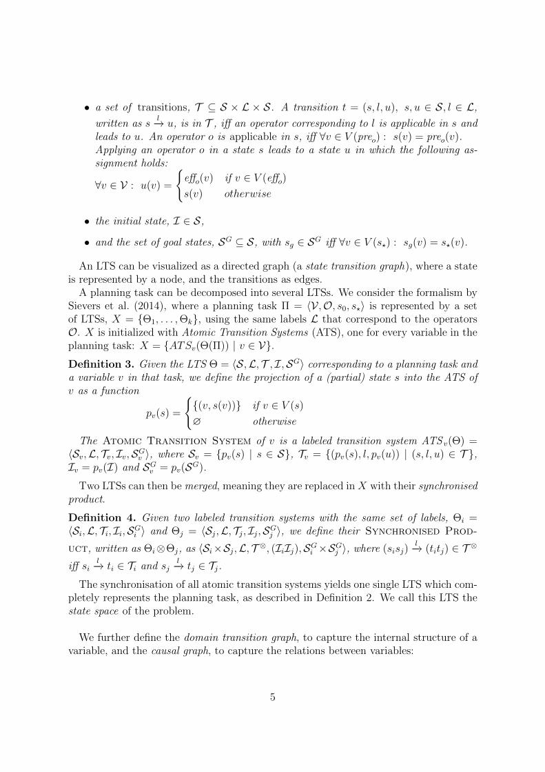
• a set of transitions, T ⊆ S × L × S. A transition t = (s, l, u), s, u ∈ S, l ∈ L,
written as sl−→ u, is in T , iff an operator corresponding to l is applicable in s and
leads to u. An operator o is applicable in s, iff ∀v ∈ V (preo) : s(v) = preo(v).Applying an operator o in a state s leads to a state u in which the following as-signment holds:
∀v ∈ V : u(v) =
{effo(v) if v ∈ V (effo)
s(v) otherwise
• the initial state, I ∈ S,
• and the set of goal states, SG ⊆ S, with sg ∈ SG iff ∀v ∈ V (s?) : sg(v) = s?(v).
An LTS can be visualized as a directed graph (a state transition graph), where a stateis represented by a node, and the transitions as edges.
A planning task can be decomposed into several LTSs. We consider the formalism bySievers et al. (2014), where a planning task Π = 〈V ,O, s0, s?〉 is represented by a setof LTSs, X = {Θ1, . . . ,Θk}, using the same labels L that correspond to the operatorsO. X is initialized with Atomic Transition Systems (ATS), one for every variable in theplanning task: X = {ATSv(Θ(Π)) | v ∈ V}.Definition 3. Given the LTS Θ = 〈S,L, T , I,SG〉 corresponding to a planning task anda variable v in that task, we define the projection of a (partial) state s into the ATS ofv as a function
pv(s) =
{{(v, s(v))} if v ∈ V (s)
∅ otherwise
The Atomic Transition System of v is a labeled transition system ATS v(Θ) =〈Sv,L, Tv, Iv,SG
v 〉, where Sv = {pv(s) | s ∈ S}, Tv = {(pv(s), l, pv(u)) | (s, l, u) ∈ T },Iv = pv(I) and SG
v = pv(SG).
Two LTSs can then be merged, meaning they are replaced in X with their synchronisedproduct.
Definition 4. Given two labeled transition systems with the same set of labels, Θi =〈Si,L, Ti, Ii,SG
i 〉 and Θj = 〈Sj,L, Tj, Ij,SGj 〉, we define their Synchronised Prod-
uct, written as Θi⊗Θj, as 〈Si×Sj,L, T ⊗, (IiIj),SGi ×SG
j 〉, where (sisj)l−→ (titj) ∈ T ⊗
iff sil−→ ti ∈ Ti and sj
l−→ tj ∈ Tj.The synchronisation of all atomic transition systems yields one single LTS which com-
pletely represents the planning task, as described in Definition 2. We call this LTS thestate space of the problem.
We further define the domain transition graph, to capture the internal structure of avariable, and the causal graph, to capture the relations between variables:
5
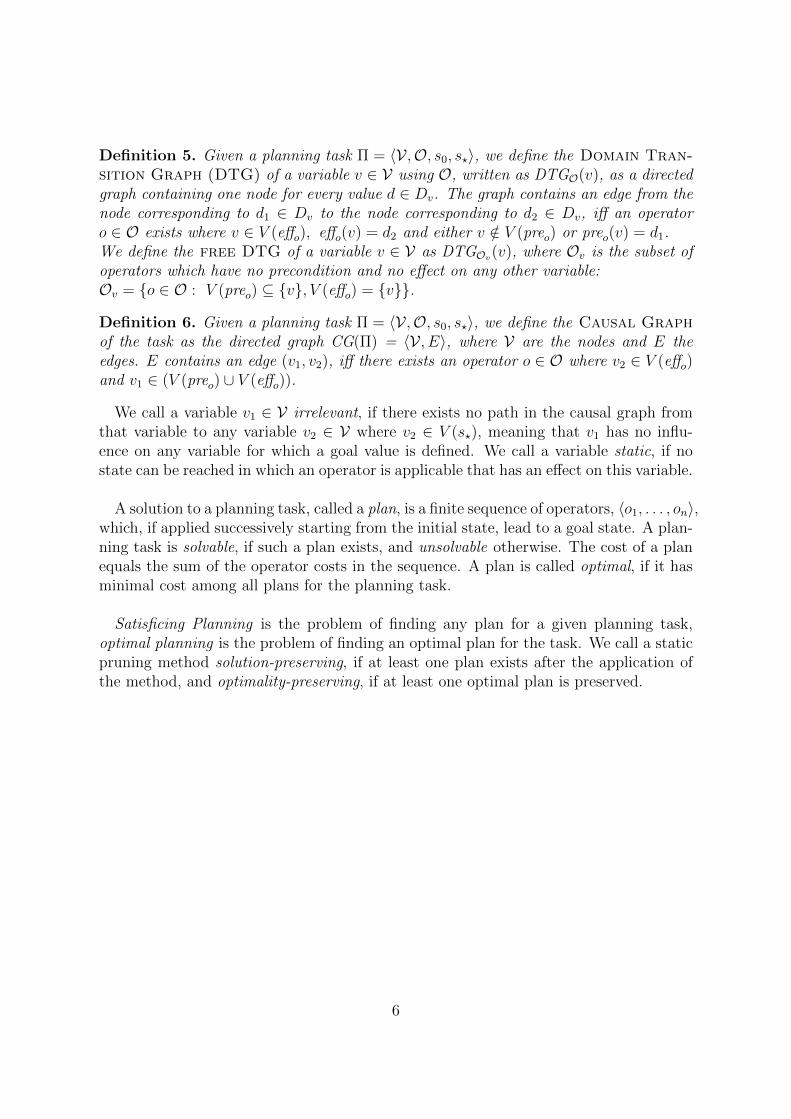
Definition 5. Given a planning task Π = 〈V ,O, s0, s?〉, we define the Domain Tran-sition Graph (DTG) of a variable v ∈ V using O, written as DTGO(v), as a directedgraph containing one node for every value d ∈ Dv. The graph contains an edge from thenode corresponding to d1 ∈ Dv to the node corresponding to d2 ∈ Dv, iff an operatoro ∈ O exists where v ∈ V (effo), effo(v) = d2 and either v /∈ V (preo) or preo(v) = d1.We define the free DTG of a variable v ∈ V as DTGOv(v), where Ov is the subset ofoperators which have no precondition and no effect on any other variable:Ov = {o ∈ O : V (preo) ⊆ {v}, V (effo) = {v}}.
Definition 6. Given a planning task Π = 〈V ,O, s0, s?〉, we define the Causal Graphof the task as the directed graph CG(Π) = 〈V , E〉, where V are the nodes and E theedges. E contains an edge (v1, v2), iff there exists an operator o ∈ O where v2 ∈ V (effo)and v1 ∈ (V (preo) ∪ V (effo)).
We call a variable v1 ∈ V irrelevant, if there exists no path in the causal graph fromthat variable to any variable v2 ∈ V where v2 ∈ V (s?), meaning that v1 has no influ-ence on any variable for which a goal value is defined. We call a variable static, if nostate can be reached in which an operator is applicable that has an effect on this variable.
A solution to a planning task, called a plan, is a finite sequence of operators, 〈o1, . . . , on〉,which, if applied successively starting from the initial state, lead to a goal state. A plan-ning task is solvable, if such a plan exists, and unsolvable otherwise. The cost of a planequals the sum of the operator costs in the sequence. A plan is called optimal, if it hasminimal cost among all plans for the planning task.
Satisficing Planning is the problem of finding any plan for a given planning task,optimal planning is the problem of finding an optimal plan for the task. We call a staticpruning method solution-preserving, if at least one plan exists after the application ofthe method, and optimality-preserving, if at least one optimal plan is preserved.
6
3. Static Pruning Methods Revisited
In this chapter, we explain three existing pruning techniques, which will be examined inthis work; two of which are solution-preserving, and one optimality-preserving. Further,we investigate some of their properties and possible extensions.
3.1. Safe Abstraction
The technique of Safe Abstractions has firstly been described by Helmert (2006). SafeAbstraction (SA) aims to abstract variables in a problem, so the search algorithm canrun on a smaller, abstracted problem without dependencies on these variables. Weformalize the abstraction of a variable from a planning task as follows:
Definition 7. Given a planning task Π = 〈V ,O, s0, s?〉 and a variable v ∈ V, we definethe effect of abstracting v from the planning task on a (partial) state s as a function
av(s) =
{s \ {(v, s(v))} if v ∈ V (s)
s otherwise
Using that function, the planning task that results from abstracting v from Π is definedas follows: SAv(Π) = 〈V \ v,O′, av(s0), av(s?)〉 where the set of operators is defined asO′ = {〈av(preo), av(effo), c(o)〉 | o ∈ O}.
A special property of Safe Abstractions is that they fulfill the downward refinementproperty: Every plan for the abstract problem can be extended into a plan for theconcrete problem, meaning no additional states are reachable in the abstract problemcompared to the concrete problem. This property is used in the formalization of SA byHaslum (2007), to define safe (safely abstractable) variables:
Definition 8. Given a planning task Π = 〈V ,O, s0, s?〉, we call a variable v ∈ V safe,if SAv(Π) fulfills the downward refinement property, meaning that a plan for SAv(Π)can be refined into a plan for Π by inserting operators from the set {o ∈ O | V (preo) ⊆{v}, V (effo) = {v}} which only depend on v and only affect v.
The original concept of SA by Helmert (2006) used the following conditions for safevariables:
Theorem 1. (Helmert, 2006)Given a planning task Π = 〈V ,O, s0, s?〉, a variable v ∈ V is safe, if its domain
7

transition graph DTGO(v) is strongly connected and v is a source node in the causalgraph CG(Π).
The intuition behind these conditions is that if a variable can arbitrarily take on anyvalue independently of any other variable, it is ensured that any plan for the problemresulting from removing that variable, called an abstract plan, can be modified to a planfor the original problem, called a concrete plan. Whenever an operator in the abstractplan has a precondition on the value of an abstracted variable, the precondition can besatisfied by inserting operators into the plan that change the variable’s value as required.If there exists a goal condition on the abstracted variable, it can be satisfied in a simi-lar way by inserting operators at the end of the abstract plan. We call this process ofmodifying an abstract plan to be a concrete plan refining the abstract plan.
The process of abstracting a set of safe variables {v1, . . . , vk} ⊆ V from a planning taskΠ = 〈V ,O, s0, s?〉 removes the safe variables and any precondition, effect, or goal condi-tion on them, creating an abstract planning task Π′ = SAvk(SAvk−1
(. . . (SAv1(Π)) . . . )).It is possible that further variables become safe in Π′ and can be abstracted, since someoperators lost dependencies they had in Π. We call this process a cascading abstraction.It can be repeated, until no more variables become safe.
The search is then executed on the most abstract planning task, yielding a plan for itif the problem is solvable. It is possible that after the abstraction process every variablewith a goal condition has been abstracted, in which case the abstract problem is solvedby a plan of zero length. No actual search is required to solve the problem in this case,we say that the problem has been solved by Safe Abstraction.Since variables which were abstracted lastly have preconditions on previously abstractedvariables, the refining of the abstract plan also needs to be performed in a successiveway, inserting the abstracted variables in the reversed ordering. With every insertedvariable, the plan becomes more concrete.
As Haslum (2007) explains, the conditions by Helmert are stronger than they needto be to make a variable safe. To ensure that every abstract plan can be refined, it isnot necessary that every abstracted variable is a source node in the causal graph, andonly a subset of the variable’s values needs to be connected in the variable’s free DTG.Haslum identifies the relevant conditions based on the following definitions:
Definition 9. Given a planning task Π = 〈V ,O, s0, s?〉 and a variable v ∈ V, we call avalue d2 ∈ Dv free reachable from another value d1 ∈ Dv, iff a path exists from d1to d2 in DTGOv(v).
We call a value d ∈ Dv externally required, iff there exists an operator o ∈ Osuch that v ∈ V (preo), preo(v) = d and V (effo) 6⊆ {v}, meaning o has d as a preconditionon v, and at least one effect on a variable other than v.
8

We call a value d ∈ Dv externally caused, iff there exists an operator o ∈ O suchthat v ∈ V (effo), effo(v) = d and V (effo) 6⊆ {v}, meaning o has d as an effect on v, andat least one effect on a variable other than v.
Theorem 2. (Haslum, 2007)Given a planning task Π = 〈V ,O, s0, s?〉, a variable v ∈ V is safe, if all externallyrequired values of v are strongly connected in its free DTG and free reachable from everyexternally caused value of v, and the goal value of v (if any) is free reachable from eachexternally required value.
The intuition behind Theorem 2 is that every value the abstract plan might requirea previously abstracted variable to have must be free reachable from every value thevariable might take on as a consequence of the plan. This ensures that whenever a valueof the variable is needed, an operator sequence exists which assigns this value to thevariable and is independent of other variables.
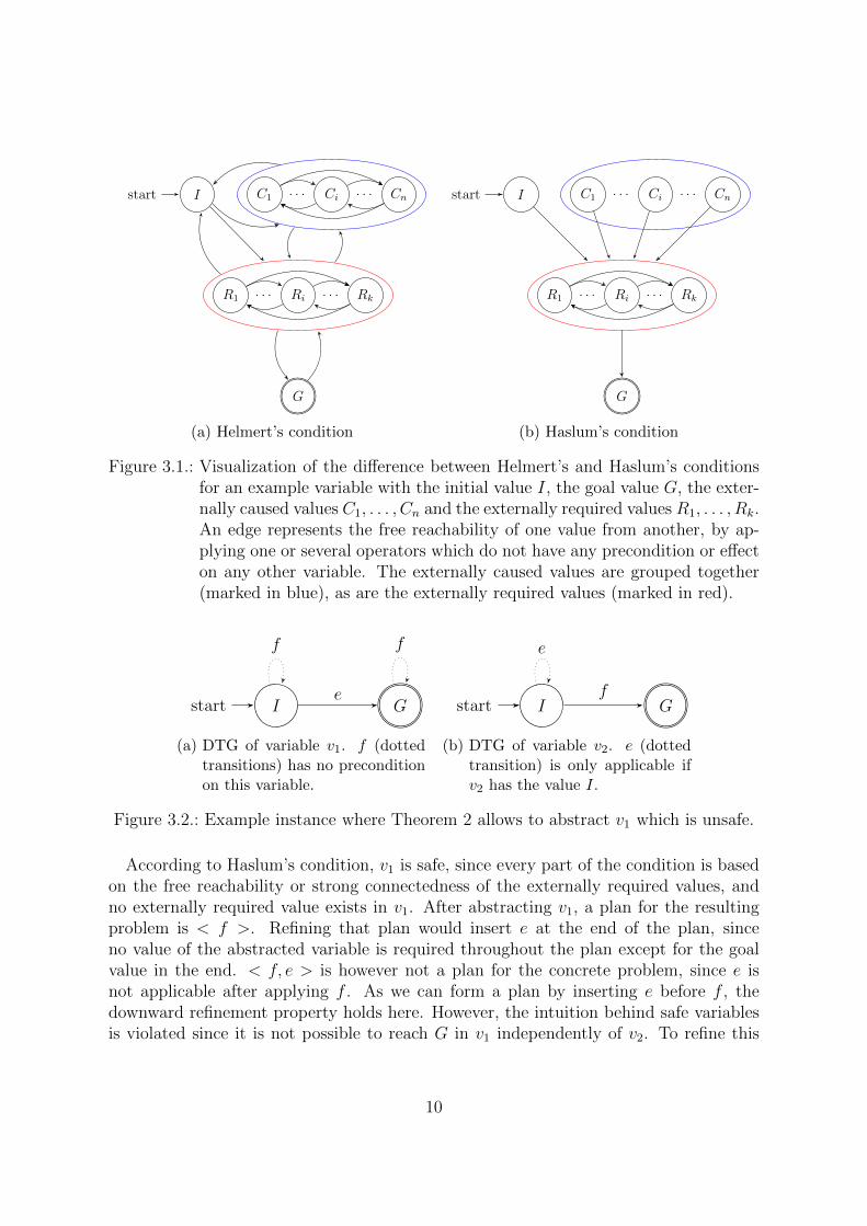
Figure 3.1 visualizes the different conditions for Safe Abstraction on the free DTGof a variable. The two depicted graphs show which structure has to exist in the freeDTG of the variable to make it safe. With Helmert’s condition, shown in Subfigure(a), the free DTG must be strongly connected, meaning that every value has to be freereachable from every other. Since free reachability is a transitive relation, at least oneof the caused/required values has to be free reachable from values outside of the group,which is depicted by a single edge to and from the group of values.As Helmert’s condition is stronger than it needs to be, some of the connections in thegraph are not necessary to make the variable safe. For example, it is not necessary thatother values are free reachable from the goal state G, since that value is only requiredat the end of the plan - except G was an externally required value.In Haslum’s condition, shown in Subfigure (b), fewer connections are required. Theinitial value and the externally caused values do not need to be free reachable, exceptthey overlap with the externally required values or contain the goal value. Similarly, thevalues of the variable do not need to be free reachable from the goal value.
Considering Theorem 2, one special case exists we’d like to discuss. When a variablehas no externally required values, and the goal value is not free reachable from the initialstate or an externally caused value, then the variable is safe according to the theorem.If it is abstracted, however, the previously described straight-forward refining algorithmis not necessarily going to produce a plan for the original problem. Figure 3.2 showsan example instance in which this applies, a planning task Π = 〈V ,O, s0, s?〉 with thevariables V = {v1, v2}, the domains Dv1 = Dv2 = {I,G}, the initial state s0 = (I, I),the goal state s? = (G,G), and the operators O = {e, f} where e has the preconditionspree(v1) = I, pree(v2) = I and the effect v1 ←− G, f has the precondition pref (v2) = Iand the effect v2 ←− G.
9
Istart C1 Ci Cn
R1 Ri Rk
G
. . . . . .
. . . . . .
(a) Helmert’s condition
Istart C1 Ci Cn
R1 Ri Rk
G
. . . . . .
. . . . . .
(b) Haslum’s condition
Figure 3.1.: Visualization of the difference between Helmert’s and Haslum’s conditionsfor an example variable with the initial value I, the goal value G, the exter-nally caused values C1, . . . , Cn and the externally required values R1, . . . , Rk.An edge represents the free reachability of one value from another, by ap-plying one or several operators which do not have any precondition or effecton any other variable. The externally caused values are grouped together(marked in blue), as are the externally required values (marked in red).
Istart Ge
f f
(a) DTG of variable v1. f (dottedtransitions) has no preconditionon this variable.
Istart Gf
e
(b) DTG of variable v2. e (dottedtransition) is only applicable ifv2 has the value I.
Figure 3.2.: Example instance where Theorem 2 allows to abstract v1 which is unsafe.
According to Haslum’s condition, v1 is safe, since every part of the condition is basedon the free reachability or strong connectedness of the externally required values, andno externally required value exists in v1. After abstracting v1, a plan for the resultingproblem is < f >. Refining that plan would insert e at the end of the plan, sinceno value of the abstracted variable is required throughout the plan except for the goalvalue in the end. < f, e > is however not a plan for the concrete problem, since e isnot applicable after applying f . As we can form a plan by inserting e before f , thedownward refinement property holds here. However, the intuition behind safe variablesis violated since it is not possible to reach G in v1 independently of v2. To refine this
10

plan correctly, the algorithm would need to look ahead, and detect that e needs to beapplied before f . In this example, v2 would be safely abstractable and v1 subsequentlywithout refinement problems, but with more than two variables this is not necessarilythe case.We propose to capture this special case with a further condition in Theorem 2: If theconsidered variable has no externally required values but a goal value, then the goalvalue must be free reachable from every externally caused value and the initial value.
3.2. Redundant Operator Reduction
The aim of the technique described by Haslum and Jonsson (2000), which we call Redun-dant Operator Reduction (ROR), is to remove redundant operators from the planningtask. An operator is called redundant, if we can replace its application in any plan by asequence of different operators and the resulting sequence, although potentially longer,will still be a plan for the problem. The state-transition graph of a problem with redun-dant operators contains many transitions which are not directly necessary to make theproblem solvable, meaning it is denser than it needs to be. Removing those operatorsresults in a decrease of the branching factor, so fewer edges have to be considered. Thiscan potentially speed up the search, as long as the solution depth (the plan length) doesnot increase too much.
The original description of the technique by Haslum and Jonsson (2000) is based onthe STRIPS problem formulation. In STRIPS, every variable is binary, and precondi-tions/goal conditions only exist on the True-value of the variables. Consequently, aneffect making a variable True can only increase the number of applicable operators,which is called an add -effect, while a delete-effect sets a variable to False and possiblycauses operator/goal conditions to not be satisfied anymore. As we consider non-binaryvariables in this work, such a split is not possible. Every effect is simultaneously an add-effect for the assigned value and a delete-effect for every other value of the variable’sdomain. For that reason, we rephrase the original definitions (Def. 3 and 4 in Haslumand Jonsson (2000)) in a SAS+ formulation.
To detect an operator o ∈ O as redundant, an operator sequence must exist thatimplements o, meaning it is applicable in all states in which o can be applied, and itmust lead to the same state o would lead to. A concept needed to define this implementsrelation is that of cumulative effects and preconditions of an operator sequence, which isdefined inductively in Definition 10: When the sequence is extended by an operator, itscumulative preconditions grow by those variable assignments which aren’t ensured by thecumulative effects of the sequence already. Only when these cumulative preconditions aremet in a state, the entire operator sequence can be applied successively. The cumulativeeffects are extended by the effects of the new operator if the sequence had no effect on
11

s
s′t
o
o1
o2
Figure 3.3.: Redundant operator: o (marked red) is implemented by 〈o1, o2〉.
the respective value, and overwritten by the new value if the sequence had an effecton this variable. The cumulative effects and preconditions together form the minimalassignment which is met after applying the operator sequence.
Definition 10. We define the cumulative preconditions and effects of a se-quence of SAS+ operators, denoted pre..., eff ... respectively, aspreo1,...,on,o = preo1,...,on ∪ {(var, val) ∈ preo | @(var, val) ∈ eff o1,...,on}eff o1,...,on,o = eff o ∪ {(var, val) ∈ eff o1,...,on | var 6∈ V (eff o)}
Definition 11. We say a sequence of operators o1, . . . , on implements an operator o,iff(i) o does not occur in the sequence,(ii) preo1,...,on ⊆ preo
(iii) eff o = eff o1,...,on
Based on Definition 11, a redundant operator can then be defined as an operator o ∈ Ofor which a sequence of operators o1, . . . , on ∈ (O\{o}) exists which implements o. Figure3.3 visualizes the state-transition graph of a problem containing a redundant operator,which is implemented by a sequence of length 2. Removing a redundant operator fromthe planning task means that a short-cut transition is removed in the state-transitiongraph, but the state is still reachable by applying a sequence of other operators, mean-ing no state is pruned: In the example, all three states are still reachable after pruning o.
Definition 11 differs from the formulation found in Haslum and Jonsson (2000) inthe third condition, where add- and delete-effects are not separable. Also, in the orig-inal version it was allowed for an operator sequence to have more delete-effects thanthe operator it implements, iff the additional values it deletes (changing the variable’svalue to false) are incompatible with the preconditions of the operator. A variable’svalue is incompatible with the preconditions, if no state can be reached in which thisvalue is assigned and the preconditions of the operator are satisfied. Consequently,deleting that value in the operator sequence does not change anything, since the valuedoes not hold. Haslum and Jonsson explain this special case with an example from
12
the Blocksworld domain. The operator Move(block A, from block B, to block C)
is redundant with the operator sequence of applying Unstack(block A, from block
B) and Stack(block A, on block C). The operator sequence has a cumulative delete-effect, ¬ ontable(block A), as the block was moved from the table onto block C. TheMove-operator does not have this delete-effect, the effect is, however, incompatible withthe precondition onblock(block A, on block B), since a block can’t be on top of an-other block and on the table simultaneously.As in SAS+ problem formulations such mutually exclusive facts are commonly expressedas different values of the same variable, the value ontable(block A) is overwritten bythe value onblock(block A, on block C) in the cumulative effects of the describedoperator sequence, which is a value the implemented Move-operator also assigns to thevariable. Therefore this special case does not need to be considered in the SAS+ formu-lation. In the case of other mutually exclusive facts which span across multiple variablesbeing known, they could be incorporated into Definition 11 as a modification of the thirdcondition: If an operator sequence o1, . . . , on has one effect on a variable, v ←− d, d ∈ Dv,on which the operator o has no effect, Definition 11 does not allow the sequence to im-plement the operator. However, if every other value e ∈ (Dv \{d}) is mutually exclusivewith at least one precondition of o, whenever o is applicable, v must already have thevalue d. In that case, permitting the additional effect of o1, . . . , on would allow to detecto as redundant. Since this exceptional case depends on the availability of additional in-formation about mutually exclusive facts, and to keep things simple, it is not consideredin Definition 11.
Haslum and Jonsson define a reduced set of operators as a set which does not containany redundant operators. Often operators are responsible for implementing each other,and by removing a redundant operator another previously redundant operator is notimplemented anymore. Depending on the order of operators removed, the size of theresulting reduced set can differ. As shown in the paper, finding a minimal reduced set isNP-hard, so in practice they make use of a greedy algorithm that removes a redundantoperator directly when it is detected. To further reduce the complexity of the algo-rithm, they define a maximum operator sequence length, and show that in the examinedinstances (Blocks, Logistics, Grid) a limit of 2 operators produces almost as smalloperator sets as higher limits do.
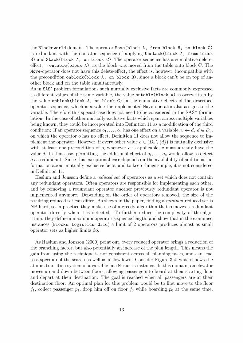
As Haslum and Jonsson (2000) point out, every reduced operator brings a reduction ofthe branching factor, but also potentially an increase of the plan length. This means thegain from using the technique is not consistent across all planning tasks, and can leadto a speedup of the search as well as a slowdown. Consider Figure 3.4, which shows theatomic transition system of a variable in a Miconic instance. In this domain, an elevatormoves up and down between floors, allowing passengers to board at their starting floorand depart at their destination. The goal is reached when all passengers are at theirdestination floor. An optimal plan for this problem would be to first move to the floorf1, collect passenger p1, drop him off on floor f3 while boarding p0 at the same time,
13

and then drop off the second passenger one floor lower.
f0start f1
f2 f3
board p1
depart p0
board p0
depart p1
Figure 3.4.: ATS of the elevator location variable in a Miconic instance. The label nota-tions at the transitions between floors have been left out, because they arenot relevant. The dotted edges correspond to operators which are removedby ROR. board pi and depart pi are operators with effects on other variablesand conditions on the elevator variable.
The elevator’s position is encoded in a variable whose values are strongly connectedin the graph of its ATS, so many redundant operators can be removed by ROR - in thisexample, it removes 8 operators. This leads to an increase in the number of states thatneed to be expanded (from 9 to 12 states), since some shortcuts, such as moving fromfloor f1 directly to f3, are not possible anymore.
The above example shows that it is not always beneficial in planning to remove aredundant operator. In that case, ROR is removing too many operators, since it onlyuses redundancy as criterion. One idea regarding this problem is that ROR could beextended with knowledge similar to what is used in the Tunnel Macros by Nissim et al.(2012). If the dynamic method of action tunneling was used after removing the redun-dant operators in this problem, it would tunnel the ascend from floor f1 to f3, sincewithout having passenger p0 boarded, there is nothing to be done on floor f2 except formoving on to a different floor. A dynamically pruning version of ROR with this knowl-edge could avoid pruning the f1 −→ f3 transition, since it is a tunnel for the implementingsequence.
14

3.3. Dominance Pruning
Another pruning method to speed up the search, recently researched by Torralba andHoffmann (2015), is Dominance Pruning (DP), which is in contrast to the previouslyexplained techniques optimality-preserving. It is based on the idea that some states arebetter to be in than others, and that a state does not need to be explored when a betterstate was previously considered already. Definition 12 describes the label-dominancesimulation that is used to define this state relation. It is calculated on labeled transitionsystems, {Θ1, . . . ,Θn}, which represent the problem, and contains those pairs of states(s, t) in an LTS where state t simulates s, written as s � t. Denoting the cost of theshortest path for a given state p to a goal state as h∗(p) (the perfect heuristic), s � tmeans that h∗(t) <= h∗(s) holds, so t is “at least as good” as s. Note, that Definition 12is based on the concept of label domination (Definition 13) and vice versa. They forma cyclic definition, which has to be accounted for using an iterative implementation.
Definition 12. (Label-Dominance Simulation). Def. 5 in Torralba and Hoffmann (2015)Let X = {Θ1, . . . ,Θk} be a set of LTSs sharing the same labels. Denote the states ofΘi by Si. A set R = {�1, . . . ,�k} of binary relations �i ⊂ Si × Si is a label-dominance simulation for X if, whenever s �i t, s ∈ SG
i implies that t ∈ SGi ,
and for every transition sl−→ s′ in Θi, there exists a transition t
l′−→ t′ in Θi such thatc(l′) <= c(l), s′ �i t
′, and, for all j 6= i, l′ dominates l in Θj given �j.We call R the coarsest label-dominance simulation if, for every label-dominance
simulation R′ = {�′1, . . . ,�′k} for X , we have �′i ⊆ �i for all i.
s s′
t t′
l
l′
sim? simdom
Figure 3.5.: State simulation according to Definition 12 for one example transition start-ing from s, for which a transition in t needs to exist which leads to a stateat least as good as s′.Whether t simulates s (sim?) depends on whether l′ dominates l in all otherLTS (dom) and whether t′ simulates s′ (sim)
Figure 3.5 visualizes the conditions for a pair of states to be an element in the label-dominance simulation: The state t simulates the state s, if for every transition from s to
15
a different state s′ there exists a transition from t to a different state t′ which simulatess′ (meaning the transition leads to a state which is at least as good as s in this LTS),and the label of the second transition dominates the label of the first transition in allother LTS.
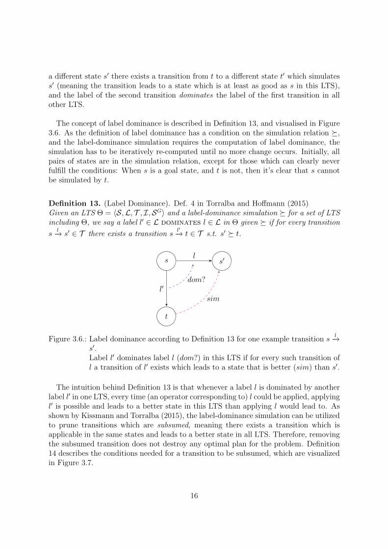
The concept of label dominance is described in Definition 13, and visualised in Figure3.6. As the definition of label dominance has a condition on the simulation relation �,and the label-dominance simulation requires the computation of label dominance, thesimulation has to be iteratively re-computed until no more change occurs. Initially, allpairs of states are in the simulation relation, except for those which can clearly neverfulfill the conditions: When s is a goal state, and t is not, then it’s clear that s cannotbe simulated by t.
Definition 13. (Label Dominance). Def. 4 in Torralba and Hoffmann (2015)Given an LTS Θ = 〈S,L, T , I,SG〉 and a label-dominance simulation � for a set of LTSincluding Θ, we say a label l′ ∈ L dominates l ∈ L in Θ given � if for every transition
sl−→ s′ ∈ T there exists a transition s
l′−→ t ∈ T s.t. s′ � t.
s s′
t
l
l′
sim
dom?
Figure 3.6.: Label dominance according to Definition 13 for one example transition sl−→
s′.Label l′ dominates label l (dom?) in this LTS if for every such transition ofl a transition of l′ exists which leads to a state that is better (sim) than s′.
The intuition behind Definition 13 is that whenever a label l is dominated by anotherlabel l′ in one LTS, every time (an operator corresponding to) l could be applied, applyingl′ is possible and leads to a better state in this LTS than applying l would lead to. Asshown by Kissmann and Torralba (2015), the label-dominance simulation can be utilizedto prune transitions which are subsumed, meaning there exists a transition which isapplicable in the same states and leads to a better state in all LTS. Therefore, removingthe subsumed transition does not destroy any optimal plan for the problem. Definition14 describes the conditions needed for a transition to be subsumed, which are visualizedin Figure 3.7.
16

Definition 14. (Subsumed Transitions). Definition 2 in Kissmann and Torralba (2015)
Given a set of LTS T = {Θ1, . . . ,Θk}, where Θi = 〈Si,L, Ti, Ii,SGi 〉, a transition si
l−→ti ∈ Ti is subsumed if and only if there exists another transition si
l′−→ t′i ∈ Ti such that
ti � t′i and l′ dominates l in all Θj for j 6= i. In that case, we say that transition sl−→ t
is subsumed by sl′−→ t′.
si ti
t′i
l
l′dom
sim
Figure 3.7.: A subsumed transition according to Definition 14.
sil−→ ti (marked in red) is subsumed by the transition si
l′−→ t′i if t′i simulatesti, and l′ dominates l in all other LTS.
In some cases, the pruning of transitions allows to remove entire operators from theplanning task if the corresponding label in a transition system becomes dead, meaningthere exist no more transitions of that label. That makes it possible to use DP as a staticpreprocessing method, while maintaining at least one optimal plan for the problem.As mentioned in Kissmann and Torralba (2015), we can obtain a coarser simulation byadding a noop-Operator without costs, that is applicable in every state and leads to nostate change. Transitions which only lead away from good states to worse ones can thenbe subsumed by noop-Transitions.By merging the labeled transition systems successively, potentially more transitions canbe detected to be subsumed. Instead of then recomputing the entire simulation on thenew set of LTS, Kissmann and Torralba (2015) suggest an incremental computation, inwhich only the simulation of the new LTS is computed. This strategy saves a lot of com-putation overhead, although with the drawback of obtaining a less coarse simulation.Also, the simulation relation does not need to be computed for every state pair in thenew LTS, the relation of some of them can be concluded from the known simulation inthe LTS which are being merged. Assume two LTS Θi and Θj are merged, and the sim-ulation for a state pair (s, t) is to be determined, where s and t are the synchronizationsof states in the two merged LTS: s = (s1s2), t = (t1t2), s1, t1 ∈ Si, s2, t2 ∈ Sj. It is asufficient criterion for s �ij t, if s1 �i t1 and s2 �j t2 holds. If one of the relations doesnot hold, the simulation needs to be computed for the state pair.
17

One important question when using DP as a static preprocessing method is when sub-sequent pruning of entire operators is solution- and optimality-preserving. As Kissmannand Torralba (2015) point out, after pruning a single subsumed transition it is in generalnot safe to prune further transitions which were previously detected to be subsumed.We try to answer the question when subsequent pruning is safe in the following theorem.
Theorem 3. A subsumed transition tx is still subsumed after pruning a subsumed tran-sition tr, except tr was only subsumed by tx.
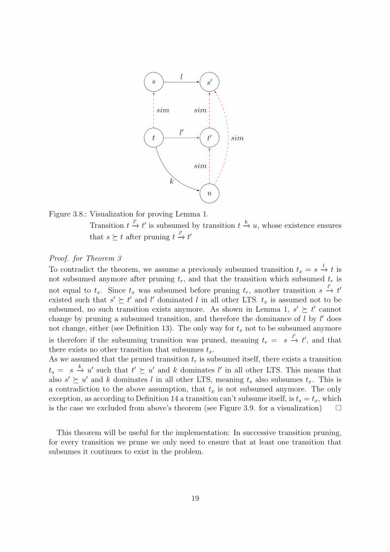
Lemma 1. Pruning a subsumed transition tr does not remove any state pairs from thelabel-dominance simulation �.
Proof. for Lemma 1We assume the contrary, i.e. there exists a state pair (s, t) ∈ � which is not in � after
pruning tr. According to Definition 12, (s, t) is in �, if for every transition sl−→ s′ a
transition tl′−→ t′ exists such that s′ � t′, l′ has less or equal costs than l and dominates
l in all other LTS.
If (s, t) was in � and is no longer in it after pruning tr, there must exist a transition
sl−→ s′, for which after pruning tr no longer any such transition t
l′−→ t′ exists, meaningeither s′ � t′ does not hold anymore, or l′ does not dominate l anymore in some other
LTS, or the transition tl′−→ t′ was pruned. The first two cases would assume that �
changed already for some other state pair, which has to be at some point caused by thepruning of a transition; we can assume without loss of generality that (s, t) is the first
pair for which the simulation changes. For that to be the case, for some sl−→ s′, tr needs
to be the only transition tl′−→ t′ which fulfills that s′ � t′ and l′ dominates l in all other
LTS. Once tr is pruned, no such transition exists anymore.As we assumed the removed transition tr was subsumed, that means there exists a tran-
sition ts = tk−→ u such that t′ � u and k had less or equal costs than and dominated
l′ in all other LTS. From definitions 12 and 13 we can conclude that � and the domi-nation relation are transitive, so if s′ � t′, and t′ � u, then s′ � u. Similarly for label
dominance, k must also dominate l. Therefore, for the transition sl−→ s′, ts takes over
the role of tr, as a transition tk−→ u such that s′ � u, k has less or equal costs than and
dominates l in all other LTS. That contradicts that there exists no such transition otherthan tr. Therefore, all pairs (s, t) stay in the label-dominance simulation � (see Figure3.8 for a visualization).
A very similar reasoning could be applied to show that the label-dominance simulationdoes not change at all, meaning no additional state pairs are added to it by pruning tr.We do not show it here, as it is not needed to prove the above theorem.
18
s s′
t t′
u
l
l′
k
sim
sim
sim
sim
Figure 3.8.: Visualization for proving Lemma 1.
Transition tl′−→ t′ is subsumed by transition t
k−→ u, whose existence ensures
that s � t after pruning tl′−→ t′
Proof. for Theorem 3
To contradict the theorem, we assume a previously subsumed transition tx = sl−→ t is
not subsumed anymore after pruning tr, and that the transition which subsumed tr is
not equal to tx. Since tx was subsumed before pruning tr, another transition sl′−→ t′
existed such that s′ � t′ and l′ dominated l in all other LTS. tx is assumed not to besubsumed, no such transition exists anymore. As shown in Lemma 1, s′ � t′ cannotchange by pruning a subsumed transition, and therefore the dominance of l by l′ doesnot change, either (see Definition 13). The only way for tx not to be subsumed anymore
is therefore if the subsuming transition was pruned, meaning tr = sl′−→ t′, and that
there exists no other transition that subsumes tx.As we assumed that the pruned transition tr is subsumed itself, there exists a transition
ts = sk−→ u′ such that t′ � u′ and k dominates l′ in all other LTS. This means that
also s′ � u′ and k dominates l in all other LTS, meaning ts also subsumes tx. This isa contradiction to the above assumption, that tx is not subsumed anymore. The onlyexception, as according to Definition 14 a transition can’t subsume itself, is ts = tx, whichis the case we excluded from above’s theorem (see Figure 3.9. for a visualization)
This theorem will be useful for the implementation: In successive transition pruning,for every transition we prune we only need to ensure that at least one transition thatsubsumes it continues to exist in the problem.
19

s
s′
t′
u′
l
l′
k
Figure 3.9.: Visualization for proving Theorem 3.
Transition sl′−→ t′ is subsumed by transition s
k−→ u′, whose existence ensures
that sl−→ s′ is still subsumed after pruning s
l′−→ t′
Subsumption relation is marked in green.
Another question of importance for the later implementation is whether it is beneficialto prune transitions when they are subsumed, even though the corresponding label doesnot become dead at that point. Theorem 4 prepares for that question by showing thatthe pruning of subsumed transitions can be delayed to a later point in time, at whichthe entire label becomes dead.
Theorem 4. Any subsumed transition is still subsumed after merging two labeled tran-sition systems.
Proof. Assuming a planning task represented by a set of labeled transition systems
{Θ1, . . . ,Θn}, we denote the subsumed transition by ail−→ si ∈ Ti and the subsuming
transition by ail′−→ ti ∈ Ti such that si � ti and l′ dominates l in all other LTS.
In the case that the transition system Θi, in which the transition is subsumed, is mergedwith another LTS, Θj, we can conclude from l being dominated in Θj that for every
transition ajl−→ sj a transition aj
l′−→ tj exists such that sj � tj. According to thedefinition of the synchronized product (see Definition 4), two transitions will therefore
exist in the merged LTS: (aiaj)l−→ (sisj), and (aiaj)
l′−→ (titj). As Kissmann and Torralba(2015) discussed, we can then conclude from si � ti and sj � tj that also (sisj) � (titj)holds. Together with the given label domination of l by l′ in the other LTS, whichstayed the same during the merging process, the necessary conditions for subsuming thetransition are met.
20
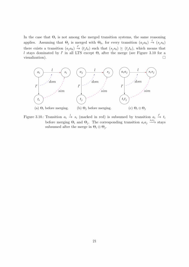
In the case that Θi is not among the merged transition systems, the same reasoning
applies. Assuming that Θj is merged with Θk, for every transition (ajak)l−→ (sjsk)
there exists a transition (ajak)l′−→ (tjtk) such that (sjsk) � (tjtk), which means that
l stays dominated by l′ in all LTS except Θi after the merge (see Figure 3.10 for avisualization).
ai si
ti
l
l′
sim
dom
(a) Θi before merging.
aj sj
tj
l
l′
sim
dom
(b) Θj before merging.
aiaj sisj
titj
l
l′
sim
dom
(c) Θi ⊗Θj
Figure 3.10.: Transition ail−→ si (marked in red) is subsumed by transition ai
l′−→ tibefore merging Θi and Θj. The corresponding transition aiaj
sisj−−→ stayssubsumed after the merge in Θi ⊗Θj.
21
4. Combinations and Synergy Effects
In this chapter we will examine the previously introduced pruning methods in combina-tion with each other. As all three techniques prune the search space in a different way,potentially an even smaller search space can be obtained by applying two techniques sub-sequently. Particularly interesting are synergies between two pruning methods, wherethe set of operators/variables pruned by the combination differs from the union of thepruning achieved by each technique individually. We say a pruning technique has a pos-itive synergy on a subsequently applied technique, if the second method benefits fromthe pruning of the first one and is able to prune more than it is able to on the originalproblem. Equivalently, a negative synergy lets the second technique prune less than itwould have been able to on the original problem, although less pruning is not considereda negative synergy when the first technique already pruned the operator/variable whichthe second method would have been able to. We abbreviate the three pruning techniquesas SA (Safe Abstraction), ROR (Redundant Operator Reduction) and DP (DominancePruning), and denote them, when applied successively to a planning task, with a plus.ROR+SA therefore describes an application of Redundant Operator Reduction, followedby Safe Abstraction.
For some of these combinations theoretical results can prove that no negative synergiesexist. In combinations where negative or positive synergies are possible, we find exampleinstances from the IPC benchmarks or construct instances in which they occur. In thischapter, we consider Haslum’s conditions for Safe Abstraction. Since the set of variablesabstracted with Helmert’s condition is a subset of the variables abstracted with Haslum’s,proofs which show that negative synergies do not exist also hold for the Helmert version.Similarly, we consider Dominance Pruning using the coarsest simulation.
22

4.1. Safe Abstraction and Redundant OperatorReduction
Negative synergies of Safe Abstraction on ROR do not occur, as Theorem 5 shows.SA+ROR allows ROR to remove all operators it could have on the original task, exceptfor those which SA already removed.
Theorem 5. The planning task resulting from the application of SA+ROR does not con-tain any operator which is not contained in the planning task resulting from applyingRedundant Operator Reduction.
Proof. We assume the contrary, i.e. there exists an operator o in the planning taskwhich is redundant, has at least one effect on a variable which is not safe abstractable(otherwise Safe Abstraction could remove this operator), and is not redundant anymoreafter applying Safe Abstraction.Then, according to the definition of redundancy as implementation by an operator se-quence, and Definition 11, there must exist a sequence of operators o1, . . . , on in theoriginal planning task which implements o, and after abstracting a variable v this is notthe case anymore. This could have the following causes:
1. The operator sequence has a (cumulative) precondition which o does not have:Clearly this means that a precondition of o was removed, as no preconditions areadded by the abstraction process. Only preconditions on v are removed by SafeAbstraction, which means the preconditions in the operator sequence on v are alsoremoved and the operator o stays redundant.
2. The (cumulative) effects of the operator sequence differ from those of o:In analogy to the preconditions, only effects on v are removed, and in both theoperator sequence and the operator o.
3. An operator oi in the operator sequence is removed by Safe Abstraction:If an operator is removed by Safe Abstraction, its only effects were on the variablev. As the preconditions on v are removed by Safe Abstraction, a shorter operatorsequence without oi now implements o and therefore o can still be removed.
Potentially, more operators can be removed by ROR after applying Safe Abstraction,as described in Theorem 6.
Theorem 6. SA+ROR can have positive synergy effects, if a sequence of operators wouldimplement an operator apart from preconditions or effects on safe variables.
23
Proof. An example that shows this type of positive synergy can be found in a Tpp
instance, where two trucks are available to move to different locations and buy goods.For each good, each location and each truck, one buy operator is available which movesthe truck to that location and loads the good into the store. After Safe Abstractionremoves the variables encoding the truck location, every two of these buy operatorsimplement each other, since they become equivalent when the location of the truck isnot stored; which results in the removal of all buy operators for one of the two trucks.
In reversed order, ROR+SA, negative synergies are again not possible as shown in The-orem 7.
Theorem 7. Safe Abstraction, executed after ROR, can abstract at least as many vari-ables as Safe Abstraction can on the original task.
Lemma 2. If there exists a variable v which is safe and an operator o which is redundant,then after removing o from the planning task, v is still safe.
Proof. for Lemma 2As explained in Theorem 2, the conditions for Safe Abstraction only depend on the freereachability of values of v. Under the assumption that after the removal of o the variableis not abstractable anymore, we can draw the conclusion that o needs to be part of thefree DTG, otherwise it could not have an effect on the safe abstractability.Being part of the free DTG of v, o does not have any precondition nor effect on anyother variable. As o was assumed to be redundant, it is implemented by a sequence ofoperators o1, . . . , on, which, according to Definition 11, cannot have preconditions noreffects on variables o has not. Therefore the sequence o1, . . . , on is also part of the freeDTG of v. Definition 11 also ensures that o1, . . . , on is applicable in at least all thestates in which o is applicable, and leads to the same target states. That means the freereachability of states of v does not change by removing o from the planning task, and vcan still be abstracted.Theorem 7 directly follows from Lemma 2.
Positive synergies of ROR+SA are not straight-forward to see, but do exist as the fol-lowing theorem shows.
Theorem 8. ROR+SA can have positive synergy effects, if redundant operators are re-sponsible for values in a variable being externally caused or required.
Proof. Figure 4.1 shows an example of a Pegsol problem instance where positive syner-gies are possible. We examine the DTG of a variable which keeps track of the last movethat was made, omitting the details about other variables for the sake of simplicity.The straight edges resemble operators which belong to the free DTG of the variable,
24

while the dotted edges mark operators with effects or preconditions on other variables(external operators).
move− endedstart
0− 2
0− 4
1− 21− 4
2− 2
2− 4
. . .
(a)
move− endedstart
0− 2
0− 4
1− 21− 4
2− 2
2− 4
. . .
(b)
Figure 4.1.: DTG of a variable from a Pegsol instance that becomes safe after removingredundant operators. The labels corresponding to the transitions are notdenoted in the graphs, since they are irrelevant.
The centered value move− ended (a, marked in red) is externally required by the ex-ternal operators which lead to the other values in this DTG (bent dotted edges), makingthose values externally caused. The other values in the DTG are also externally required
25

by the external operators which connect them with each other in this DTG (straightdotted edges). The variable is not safe abstractable, since the externally required valuesmarked in purple are not free reachable from the move− ended value.All connections of the outer values (straight dotted edges) are redundant with a detourto the center value, therefore ROR can remove them. After removing the redundantoperators, the outer values are not externally required anymore (b, marked in blue),hence they do not need to be free reachable from the move− ended value. The variablebecame safe.
4.2. Dominance Pruning and Safe Abstraction
The following two sections explore the application of Dominance Pruning in combina-tion with a satisficing pruning technique. The consequence of such combination is thatthe optimality-preserving property of Dominance Pruning is lost. A decrease in timeneeded to solve instances this way is not to be expected, since the gain of an optimality-preserving method applied to domains used for satisficing planning is often too smallcompared to the overhead. Still, it is of interest to investigate their relative pruningcapacities, including potential synergies, on a conceptual level. In this section, we in-vestigate DP combined with SA.
The combination of SA+DP removes at least the same operators from the problem asjust applying DP does: Theorem 9 shows this by proving that no operator can exist in aproblem which DP is able to prune, and that is still existent and not prunable anymoreafter applying SA. Since DP does not actively remove any variables from the problem,but variables can become static if the relevant operators are pruned, the same can besaid for variables: The combination of SA+DP never leaves behind a variable which couldhave been removed if just DP had been applied.
Theorem 9. Applying SA+DP removes at least the same operators from the planningtask as only applying DP to it does.
Proof. Let X = {Θ1, . . . ,Θn} be a set of LTS representing a planning task, and letΘi ∈ X be the atomic transition system of an abstracted variable vi. In all other LTS
Θj 6= Θi, Safe Abstraction only removes those transitions sjl−→ tj ∈ Tj which belong to
an operator it removed. Safe Abstraction only removes an operator from the problem ifit had no effect and no precondition on any non-abstracted variable. Since the removedoperators had no condition and no effect on any of the remaining variables, the removedlabels were dominated by the noop-label in all Θj 6= Θi. This means that the state sim-ulation relation �j does not change in any Θj 6= Θi, since for every removed transitionthere exists a noop-transition with the same origin, destination, and equal or less cost.
26
Assume Theorem 9 to be false, i.e. there exists an operator o which can be prunedby DP in the original planning task, but not anymore after Safe Abstraction has beenapplied abstraction, and it has not been removed by Safe Abstraction. This means atransition must exist which was previously subsumed, but is not subsumed anymoreafter Safe Abstraction was applied.A transition to is not subsumed anymore according to Definition 14, if either the simu-lation relation changed, or the subsuming transition is not existent anymore. As shownabove, the simulation relation is unchanged. Further, if to was previously subsumedby a transition tSA that has been removed by Safe Abstraction, it has to be subsumedby a noop-transition tnoop now, since tSA was subsumed by tnoop, and the subsumptionrelation is transitive (since label domination and state simulation are transitive).
So, if a transition was subsumed before abstracting vi and its corresponding operatorwas not removed by Safe Abstraction then it is still subsumed after the abstractionprocess. That means abstracting one variable does not reduce the set of operators thatcan be removed from the planning task by DP, and therefore abstracting an arbitraryamount of variables does not do so, either, which proves Theorem 9.
Positive synergies of Safe Abstraction on DP are possible, meaning Dominance Prun-ing is able to prune operators it couldn’t have otherwise.
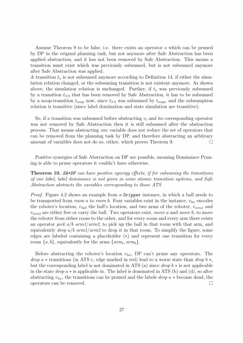
Theorem 10. SA+DP can have positive synergy effects, if for subsuming the transitionsof one label, label dominance is not given in some atomic transition systems, and SafeAbstraction abstracts the variables corresponding to those ATS.
Proof. Figure 4.2 shows an example from a Gripper instance, in which a ball needs tobe transported from room a to room b. Four variables exist in the instance, vloc encodesthe roboter’s location, vball the ball’s location, and two arms of the roboter, varm1 andvarm2 are either free or carry the ball. Two operators exist, move a and move b, to movethe roboter from either room to the other, and for every room and every arm there existsan operator pick a/b arm1/arm2, to pick up the ball in that room with that arm, andequivalently drop a/b arm1/arm2 to drop it in that room. To simplify the figure, someedges are labeled containing a placeholder (∗) and represent one transition for everyroom {a, b}, equivalently for the arms {arm1, arm2}.
Before abstracting the roboter’s location vloc, DP can’t prune any operators. Thedrop a ∗ transitions (in ATS c, edge marked in red) lead to a worse state than drop b ∗,but the corresponding label is not dominated in ATS (a) since drop b ∗ is not applicablein the state drop a ∗ is applicable in. The label is dominated in ATS (b) and (d), so afterabstracting vloc, the transitions can be pruned and the labels drop a ∗ become dead, theoperators can be removed.
27

room astart room b
move b
move a
pick a ∗, drop a ∗
pick b ∗, drop b ∗
(a) ATS of vloc, which is safely abstractable.The transitions resembled by dottededges modify only the other variables.The move ∗ transitions are applicable inany state of the other LTS, and are notdrawn there.
freestart
carry
pick ∗ arm1drop ∗ arm1
(b) Atomic Transition Systems ofvarm1
room astart robby room b
pick a ∗
drop a ∗ pick b ∗
drop b ∗
(c) Atomic Transition System of vball.
freestart
carry
pick ∗ arm2drop . . .
(d) Atomic Transition Systems ofvarm2
Figure 4.2.: Example of a positive synergy of SA on DP from the Gripper domain.
In the reverse direction, DP+SA, both positive and negative synergies are possible, asshown in Theorem 11 and 12.
Theorem 11. DP+SA can have positive synergy effects, where a variable becomes safe bypruning operators.
Proof. Figure 4.3 visualizes a positive synergy in a constructed example. The instancecontains two variables, v1 and v2, whose ATS are depicted in (a) and (b). The operatorsf1, f2, f3, f4 do not have any precondition or effect on v2, and are not depicted in thesubfigure (b) since they’re applicable in each of the states. Equivalently, the operatorsf5, f6, f7 are not drawn in the ATS 1.If Safe Abstraction is applied to that example, it is not able to abstract any variable, but
28

v1
Ystart
Z
X
TG
p
s f1
f2
e
f3
f4
(a) ATS 1 before pruning.
v2
Astart
C
B
D
G
p
s
f5
e
f6
f7
(b) ATS 2 before pruning.
v1
Ystart
Z
X
TG
s f1
f2 f3
f4
(c) ATS 1 after pruning.
v2
Astart
C
B
D
G
s
f5 f6
f7
(d) ATS 2 after pruning.
Figure 4.3.: Constructed example to show the positive synergy of DP on SA.Externally required values are marked in red, externally caused values inblue.
after applying Dominance Pruning it can do so. v1 is not safe (a), as the goal value G isnot free reachable from the externally caused value X. v2 is also not safe (b), as the ex-ternally required value A is not free reachable from the externally caused values B and C.
Transition Yp−→ X is subsumed in ATS 1 by Y
s−→ Z, and the label s dominates labelp in ATS 2, so after applying Dominance Pruning, p becomes dead in this LTS. Aftermerging the two transition systems it is possible to prune the operator e as well.
29
After pruning the p transition in ATS 1 (c), X is not externally caused anymore,with the consequence that v1 becomes safe: Y is free reachable from Z, and G is freereachable from Y. v2 is still not safe (d), as the goal value G is not free reachable fromthe externally required value A, although the variable becomes safe after abstractingv1.
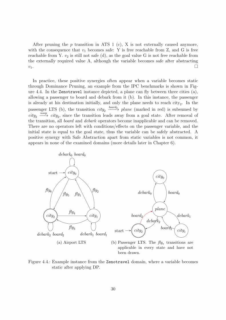
In practice, these positive synergies often appear when a variable becomes staticthrough Dominance Pruning, an example from the IPC benchmarks is shown in Fig-ure 4.4. In the Zenotravel instance depicted, a plane can fly between three cities (a),allowing a passenger to board and debark from it (b). In this instance, the passengeris already at his destination initially, and only the plane needs to reach city2. In the
passenger LTS (b), the transition city2board2−−−→ plane (marked in red) is subsumed by
city2noop−−→ city2, since the transition leads away from a goal state. After removal of
the transition, all board and debark operators become inapplicable and can be removed.There are no operators left with conditions/effects on the passenger variable, and theinitial state is equal to the goal state, thus the variable can be safely abstracted. Apositive synergy with Safe Abstraction apart from static variables is not common, itappears in none of the examined domains (more details later in Chapter 6).
city1
city0start
city2
fly1fly2
fly3
fly4
fly5fly6
debark1 board1
debark0 board0
debark2 board2
(a) Airport LTS
city0
city1city2start
plane
board0debark0
board1
debark1board2
debark2
(b) Passenger LTS. The fly∗ transitions areapplicable in every state and have notbeen drawn.
Figure 4.4.: Example instance from the Zenotravel domain, where a variable becomesstatic after applying DP.
30
wp0
wp1 wp2
wp3start
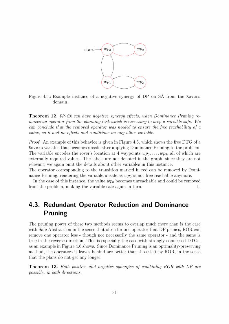
Figure 4.5.: Example instance of a negative synergy of DP on SA from the Rovers
domain.
Theorem 12. DP+SA can have negative synergy effects, when Dominance Pruning re-moves an operator from the planning task which is necessary to keep a variable safe. Wecan conclude that the removed operator was needed to ensure the free reachability of avalue, so it had no effects and conditions on any other variable.
Proof. An example of this behavior is given in Figure 4.5, which shows the free DTG of aRovers variable that becomes unsafe after applying Dominance Pruning to the problem.The variable encodes the rover’s location at 4 waypoints wp0, . . . , wp3, all of which areexternally required values. The labels are not denoted in the graph, since they are notrelevant; we again omit the details about other variables in this instance.The operator corresponding to the transition marked in red can be removed by Domi-nance Pruning, rendering the variable unsafe as wp0 is not free reachable anymore.
In the case of this instance, the value wp0 becomes unreachable and could be removedfrom the problem, making the variable safe again in turn.
4.3. Redundant Operator Reduction and DominancePruning
The pruning power of these two methods seems to overlap much more than is the casewith Safe Abstraction in the sense that often for one operator that DP prunes, ROR canremove one operator less - though not necessarily the same operator - and the same istrue in the reverse direction. This is especially the case with strongly connected DTGs,as an example in Figure 4.6 shows. Since Dominance Pruning is an optimality-preservingmethod, the operators it leaves behind are better than those left by ROR, in the sensethat the plans do not get any longer.
Theorem 13. Both positive and negative synergies of combining ROR with DP arepossible, in both directions.
31

f0start f1
f2 f3
(a) Original DTG
f0start f1
f2 f3
(b) ROR (also ROR+DP)
f0start f1
f2 f3
(c) Dominance Pruning
f0start f1
f2 f3
(d) DP + ROR
Figure 4.6.: Example Miconic instance, showing the overlapping pruning/reducing ofDP and ROR. The labels corresponding to the transitions are not denoted,since they are irrelevant.(a) DTG of the variable encoding the elevator’s location.(b) Applying ROR to the problem thins out the strongly connected DTG,after which DP is not able to prune anything.(c) Applying Dominance Pruning first, it is detected that a return to thestate f0 is not necessary and the operators leading to it can be pruned.(d) When ROR is applied after DP, it again thins out the DTG, the samenumber of operators stays in the problem as when just using ROR, but theplan can potentially be shorter, as reaching f2 from f3 does not need thedetour over f0 as it does in (b).
We do not show examples of these synergies here, since that would require to explainthe label-dominance simulation in detail for instances with a bigger number of variables.
One interesting case to look at are the positive synergies of DP on ROR, which areonly possible when by pruning an operator a variable becomes static and can be removed.In that case, it is possible for an operator to become redundant, if its conditions/effectsdiffered only on that variable from the cumulative conditions/effects of a now imple-menting sequence, and since the variable is removed, the sequence is able to implementthe operator. Otherwise, positive synergies are not possible, as shown in Theorem 14.
32

Theorem 14. An operator o, which is not redundant, cannot become redundant byapplying DP to the problem, except a variable becomes static and can be removed.
Proof. The effect of DP on the planning task, if no variable becomes static, is a reductionof the set of operators O to O′. As o is assumed not to be redundant, no sequence ofoperators in O exists which implements it, and since O′ ⊆ O, no such sequence can existin O′.
4.4. Summary on Synergy Effects
To conclude this chapter, we summarize the information gathered about the synergies.Consider Table 4.1, which lists each of the combinations.
Combination Positive Synergies Negative SynergiesSA+ROR yes noROR+SA yes noSA+DP yes noDP+SA (yes) yesROR+DP yes yesDP+ROR (yes) yes
Table 4.1.: Summary of synergy effects. Parenthesized entries indicate a synergy whichis often or always caused by variables becoming static.
Positive synergies exist for each combination, and appear in instances of the IPCbenchmarks. In DP+SA, the synergies are limited on these benchmarks in the sense thatDP often makes variables safe when it also makes them static. In DP+ROR, a variable hasto become static to cause positive synergies. Negative synergies are possible betweenROR and DP in either direction, but also in DP+SA.
Considering the benefit for the search, we can conclude from these synergies whichtechnique should preferably be applied first to the problem.For both SA+ROR and ROR+SA no negative synergies exist, and both allow positive syner-gies. Since removing redundant operators is not consistently beneficial for the search asshown in Section 3.2, it can be argued that the positive synergies of ROR+SA are likelyto be more important for reducing search effort than the positive synergies of SA+ROR.Since DP+SA allows negative synergies, and the positive synergies are rare, SA+DP shouldbe able to remove more variables and operators from any planning task. Additionally,abstracting variables before running Dominance Pruning has the benefit of speeding upthe heavy simulation computation.
33

Both ROR+DP and DP+ROR allow negative synergies, the positive synergies in DP+ROR how-ever are very infrequent. Additionally, similarly to SA+ROR, it can be argued that thepositive synergies on DP are more important than the positive synergies on ROR sinceDP does not cause an increase in the plan length.
34

5. Implementation
In this chapter, we describe the implementation of Safe Abstraction, Redundant Oper-ator Reduction and Dominance Pruning as static preprocessing methods into the FastDownward (Helmert, 2006) planning system. Fast Downward is a propositional plannerwhich consists of three components: The Translator takes as input a problem descrip-tion specified in PDDL and translates it into a SAS+-like (Backstrom and Nebel, 1995)formalism using finite-domain state variables. The Preprocessor performs a relevanceanalysis, removes irrelevant and static variables, and computes data structures such asthe causal graph and the domain transition graphs. The Search component then runsheuristic search on the output of the preprocessor.
5.1. Safe Abstraction
Although Haslum (2007) describes other preprocessing methods than Safe Abstraction- Reformulation of problem descriptions and composition of operators - they have notbeen implemented in this work, as they were at least partly performed manually and itis not clear whether and how they can be fully automated.
Safe Abstraction has been implemented into the preprocessor component of FastDownward, since after abstracting, some data structures need to be computed, for whichmethods are available in that component. The translator output file is parsed, and thedata is being stored inside a task object, which is then passed on to the abstraction.
For every variable of the task the conditions for safe abstractability are checked. Atthis point, the two conditions for Safe Abstraction demand different properties: The onedescribed by Helmert (2006) requires all values in the variable to be strongly connected,and the variable to be a source node in the causal graph. Haslum (2007) also needs atest for connectedness and reachability, but with only a selection of the values. For thatpurpose, the operators are separated into external operators, which have an effect onanother variable than the examined one, and internal operators, which have no condi-tion nor effect on other variables. The values of the variable’s domain are separated intoexternally required (precondition to an external operator) and externally caused (effectof an external operator, or initial state value).To detect whether each externally required value and the goal value are free reachablefrom all externally required and caused values, graph connectedness algorithms, such as
35

the one by Tarjan (1972), can be used. While Helmert’s condition can be implementedstraight-forwardly with an algorithm for strong connectedness, it is not as easy to cap-ture all relevant cases in Haslum’s condition. For that reason, this implementation usesan algorithm that creates a 2-dimensional array whose entries represent free reachability.Every value is free reachable from itself, and every internal operator further adds reacha-bility entries. As reachability is a transitive relation, the filling of the array was realizedas a recursive method. The reachability-array approach has a higher complexity thanTarjan’s algorithm, but it can easily be adapted to check either of the two conditions.
If at least one variable can be abstracted, a new task is generated in which the ab-stractable variables as well as conditions and effects of operators and goal conditions onthese variables, along with entries in mutually exclusive groups, are removed. Since byabstracting variables, other variables can become safe, the conditions for safe variablesare then again evaluated on all variables in the new task object, a repetitive process untileither no more variable can be abstracted or no more goal conditions remain (meaningthe problem is solved without search). Thus, each time the problem is abstracted, a newtask is created, which is stored inside a task vector.To be able to later on refine the abstract plan found by the search, the information isneeded which variable was abstracted in which order, and which operator has precondi-tions and effects on the abstracted variables. For that reason, each abstracted task inthat vector is saved to a file. As the preprocessor automatically performs a relevanceanalysis for the remaining variables, it is possible that an abstracted problem loses vari-ables which weren’t directly abstracted. These irrelevant variables cannot be part of anyplan, though.The process of refining an abstract plan loads the vector of abstracted tasks, and tra-verses the abstract plan (also loaded from a file output by the search engine) once foreach abstraction layer. It detects which variables have been abstracted, and keeps trackof them with a variable-value mapping, which is updated every time an operator in theplan requires the variable to change its value. When such a precondition on the variableexists, an operator sequence is inserted into the plan right before the value is needed.This operator sequence is determined by finding the shortest path (using the algorithmby Dijkstra (1959)) from the variable’s old value to its new one in the free domain tran-sition graph. The same procedure is done after traversing the plan, adding operatorsequences to the end of it to ensure that every abstracted variable gets assigned its goalvalue.
Complexity Analysis of the Implementation
The complexity of determining whether a variable is abstractable is dominated by thefree reachability analysis. In the recursive array implementation used, assuming nv asthe size of the variable domain, there are maximally nv(nv − 1) write operations on thearray, as the diagonal is already filled (every value is reachable from itself). For every
36

write operation, all possible predecessors of the source, and all possible successors ofthe target need to be read, leading to O(2(nv − 1)) reads per write operation. There-fore, the total complexity is dominated by the number of write operations, which isO(nv(nv − 1) ∗ 2(nv − 1)) = O(n3
v). If Tarjan’s strongly connectedness algorithm wasused for Helmert’s condition, this complexity could be reduced to O(nv + n2
v).In the worst-case, every variable can be abstracted, but each one only after the previoushas been abstracted. With v variables that leads to v+(v−1)+(v−2)+ · · ·+1 = v∗(v+1)
2
abstractability checks, meaning a total complexity for the abstraction process of O(v2n3v)
or, with Tarjan’s algorithm, O(v2n2v).
Refining a plan requires to loop through the abstract plan once for every abstractionlayer but the last one. Each iteration, for each operator in the plan, the preconditionsand effects on each abstracted variable need to be considered. In the worst case, eachoperator in the plan has a precondition on each abstracted variable, so the shortestoperator sequence from the old to the new value of that variable needs to be found.The shortest-path algorithm from Dijkstra has a complexity of O(n2
v), leading to a totalcomplexity of O(v ∗ p ∗ n2
v) with p as the maximum plan length of the refined plan.
37
5.2. Redundant Operator Reduction
The implementation of Redundant Operator Reduction is for the most part straight-forward. Same as Safe Abstraction, it is located in the preprocessor part of Fast Down-ward.In a first preparation step, the effects and preconditions of operators are transformedfrom condition/effect vectors into maps using the variable as key. This allows for fasterand simpler access later on.Then, for every operator o in the problem, a recursive method is called to look for an im-plementing operator sequence, using the operator sequence limit as maximum recursiondepth. It takes a sequence 〈o1, . . . , oi〉 as parameter, evaluates whether the sequence ful-fills the conditions of implementing o (Definition 11), and returns the sequence if that’sthe case. The conditions used differ from those found by Haslum and Jonsson (2000),where an implementing operator sequence is allowed to have additional effects whichare incompatible with preconditions of o. Because of the multi-valued domain variablesand the mutually exclusive value detection of the translator, most of these incompatiblevalue pairs appear in the problem as two values of one variable, so e.g. in the previouslydescribed Blocks example, the deletion of the axiom ontable(block) is implicitly con-tained in the move operation.The method is initially called with an empty operator sequence 〈〉. If the conditionsfor implementation of o are not satisfied by the given sequence, the method tries outevery possibly applicable operator (which doesn’t contradict a cumulative effect of thesequence up to that point), except for o, appends the new operator to the sequenceand accumulates the cumulative effects and preconditions before recursively calling it-self again. One criterion to abort appending operators to the sequence, besides therecursion depth, is when a precondition of an operator is neither a precondition of o, noris it ensured by a cumulative effect of the operator sequence, because this sequence cannever be extended to one which implements o (Haslum and Jonsson, 2000).It is important to note that this is a greedy implementation, which can produce verydifferent results on the same planning task depending on the order of operators.
Complexity Analysis of the Implementation
Let d be the maximum recursion depth (being the maximum length of an implement-ing operator sequence), nv the number of variables and no the number of operators.Then, the recursive method to find an implementing operator sequence is externallycalled exactly no times (once for every operator), calling itself (no − 1) ∗ (no − 2) ∗ · · · ∗(no − d) = (no − d+1
2)d times for each in the worst case. Each call, the cumulative
effects/preconditions need to be compared to the effects/preconditions of the operatorwhich is to be implemented. In the worst case, the operator and the operator sequencehave effects/preconditions on every variable (so nv in total), leading to a total complexityfor the reduction of operators of O(no ∗ (no − d+1
2)d ∗ nv) = O(nd+1
o ∗ nv).
38
5.3. Dominance Pruning
Unlike the other techniques, Dominance Pruning was implemented into the search com-ponent of Fast Downward because much of the required functionality regarding transitionsystems could be reused from the implementation of the Merge&Shrink heuristic. Nev-ertheless, it is implemented as a static preprocessing method. Therefore it effectivelyonly removes operators, whose labels become dead, and outputs a problem descriptionwithout them.The implementation used in this work is based on the algorithm described by Kissmannand Torralba (2015). The label-dominance simulation is initialized with all pairs ofstates, except for goal states which can’t be simulated by non-goal states. State pairsare then removed successively if they do not fulfill the conditions for simulation, aniterative process until the simulation does not change anymore. Once the simulationis computed, the subsumed transitions can be identified. As Kissmann and Torralba(2015) point out, it is in general not safe to prune subsumed transitions successively.When pruning a transition, the label-dominance simulation can change. To avoid hav-ing to recompute it, they do not prune transitions which could cause such change. Forexample, it is in general not safe to prune a transition of label A in one LTS, that isonly subsumed by a transition of label B, and later remove label B from the planningtask because it became dead in a different LTS.Such caution is necessary when single transitions of a label are pruned. However, in ourapplication of Dominance Pruning as a static preprocessing method, it is not beneficialto prune single transitions if the corresponding label does not become dead. Althoughwe then wouldn’t need to take those transitions into account in recomputations of thesimulation, directly pruning them has the drawback that mutually subsuming transi-tions cannot be pruned at all, as mentioned above. To maximize the achievable pruningof operators, the implementation used does not prune single transitions but an entirelabel from the problem, if all of its transitions in one LTS are subsumed by transitionsof other labels.
Theorem 3 shows that it is safe to prune several subsumed transitions successively,if we ensure that for each one at least one subsuming transition continues to exist. Inpractice, this is realized by storing a list of (subsumed, subsuming) transition pairs.When every transition of a label in one LTS is subsumed, the label is removed from theplanning task together with all of its transitions. Since we don’t allow transitions ofthe same label to subsume each other, all transitions of one label can be safely removedsuccessively as they are subsumed by transitions which still exist. After the removal,the list of subsumed transitions is cleaned from those transitions which were subsumedby a just-removed transition. This ensures that we prune no further transition whichis not subsumed anymore. As an example, if two transitions subsume each other, andthe label of the first transition is removed because all its transitions are subsumed, thesecond transition is not subsumed anymore, and the second label stays - except if there
39
was a third transition subsuming both of these transitions, in which case it is possibleto also remove the second label.One might think that by not pruning transitions right away when they are subsumed,information about subsumed transitions might be lost. Theorem 4 shows, though, thatsubsumed transitions stay subsumed throughout the merging process, and therefore wecan wait with the pruning until the entire label becomes dead without losing information.
In difference to Kissmann and Torralba (2015), who compute the coarsest simulationbefore the first merging step yet only prune transitions after it, this implementationdoes perform pruning on the atomic transition systems. After the pruning step, twoLTS are merged together using the DFP merging strategy (Sievers et al., 2014), andlabels are reduced if possible. Exact shrinking is not used, since it potentially reducesthe number of operators pruned, and irrelevance pruning is not performed during thepruning, either.The label-dominance simulation then needs to be updated. Kissmann and Torralba(2015) suggest to use an incremental computation: Instead of recomputing the coarsestsimulation for all LTS after every merge step, only the simulation for the new LTS iscomputed. Only when all LTS are merged together, the coarsest simulation is com-puted. This reduces the work needed for pruning, but has the potential downside ofmissing subsuming transitions because the intermediate simulations are not the coarsestpossible. Only after the final merge, the coarsest simulation is computed - but if thepruning method time-outs before that, the pruning achieved is smaller. In this imple-mentation, both versions were used; the one always calculating the coarsest simulation,to determine how much more pruning is possible, and the one using the incrementalcomputation, which would be more viable in practice.The mapping of reduced labels to the corresponding operators is stored during the merg-ing process. Since reduced labels are locally equivalent in a merged LTS, in case onelabel becomes dead in an LTS it can be translated back to the corresponding operators,which are then removed from the planning task.One option that was added in this implementation is to ignore the label costs, meaninga transition can be subsumed by a transition of a label with higher costs. Clearly, opti-mality of DP is lost using this option, but the pruning power could increase.
Potentially, after removing an operator, a variable can become static and be removedin the preprocessor, and certain data structures such as the causal graph have to berecomputed. For that reason, the dominance pruning component writes an output filein the format of the translator output, containing the planning task without the prunedoperators. This output file can then be read from the preprocessor which is thus runtwo times, once before dominance pruning and once before the search.
40
Complexity Analysis of the Implementation
The most complex component of dominance pruning is the coarsest dominance simu-lation computation. As described by Torralba and Hoffmann (2015), the simulation isinitialised with every two states simulating each other, except for goal states which arenot simulated by non-goal states. Let n be the number of labeled transition systems forwhich the simulation is to be computed, t/LTS the maximum number of transitions inone LTS, s/LTS the maximum number of states in an LTS, t/s the maximum number oftransitions of a state, and t/l the maximum number of transitions of a label in an LTS.The initial state simulation relation then contains O(n× s2/LTS) state pairs which needto be checked for simulation at least once. For each state pair, in the worst case everytransition of one state needs to be compared to each transition of the other state, andfor each of these transition pairs the label dominance of the corresponding labels needsto be calculated, resulting in a complexity of O(t2/s × dom) per state pair, with dombeing the complexity of calculating the label dominance relation between two labels.To calculate this relation, in every LTS minus one every transition of one label needs tobe compared to every transition of the other label, yielding a complexity of O(n × t2/l)with the state simulation lookup being of constant complexity.The domination of one label over the other in one LTS however doesn’t need to berecomputed for every state comparison, because it can only change when a state simu-lation pair from that LTS is removed. This means if we iterate over all state pairs inone LTS before the next one, we can store all previously computed label dominations forthe other LTS and only have to recompute them for this LTS: so every label dominationonly needs to be computed once per iteration, yielding a total complexity per iterationof O(n× s2/LTS × t2/s + n× l2 × n× t2/l). Using l × t/l = t/LTS, this complexity can be
rephrased as O(n × (s2/LTS × t2/s + n × t2/LTS)), which becomes O(n × t2/LTS × (1 + n))when using the equality of s/LTS× t/s = t/LTS. Finally, we can replace n× t/LTS by thetotal number of transitions summed over all LTS, which leads to the final complexityof O(t2total) per iteration. Although theoretically, n × s2/LTS iterations are possible, inpractice after few iterations a static point is reached in which nothing changes anymore.Since with very big problems the simulation computation will probably not be finishedwithin a reasonable time and memory limit, a complexity threshold was introducedfor the implementation which always calculates the coarsest simulation, to abort thecomputation if the effort would be too great. This complexity number is calculated asn× (s2/LTS × t2/s + n× t2/LTS).
In the case of the incremental computation, only the simulation for the merged LTSneeds to be computed, as well as the label dominance relation. The complexity ofcomputing the simulation quickly increases during the merging process, though, as thenumber of states and transitions rises.
41

6. Experiments
In this chapter, the implemented techniques are evaluated in a row of experiments. Sec-tion 6.1 describes how the experiments were performed, and which values were measured.In section 6.2 we evaluate different conditions and parameters and choose those whichseem best-suited for our purposes. Those parameters are then used in the successiveexperiments in section 6.3, where we investigate synergy effects and verify how well thetheoretical results hold, and in section 6.4, where we compare the overall performanceof different combinations with each other. Finally, we measure the performance of eachpruning technique on a set of unsolvable instances in section 6.5.As in Chapter 4, we abbreviate the subsequent application of two pruning techniques asA+B, where A and B are either SA (Safe Abstraction), ROR (Redundant Operator Reduc-tion), or DP (Dominance Pruning).
6.1. Configuration
All experiments were performed on computers with Intel Xeon E5-2660 CPUs running at2.2 GHz and with a time bound of 30 minutes (if not specified otherwise) and a memorybound of 3 GB.The experiments using Dominance Pruning alone were run on the optimal InternationalPlanning Competition (IPC) tasks up to IPC2011 (46 domains with a total of 1456tasks), using A? search (Hart and Raphael, 1968) together with the LM-Cut heuristic(Helmert and Domshlak, 2009). Other experiments were run on satisficing and optimalIPC tasks up to IPC2011 (92 domains with a total of 1886 tasks) using greedy searchtogether with the FF heuristic (Hoffmann and Nebel, 2001).The time limit for the pruning techniques used is noted in seconds in the plots in brackets.If no time limit is stated, then none was used. If several techniques are combined, theneach received the time limit noted in brackets separately. When the time limit is reached,the pruning method is aborted, and the pruning information gathered up to that pointis used.
42
Measures
In plots where the domain information is relevant, instances are displayed with a symbolindicating the domain. Appendix A lists all domains used, together with the symbolrepresenting that domain in the plots.The values displayed in the plots are:
• Reduced Operators: The number of redundant operators which could be re-moved by ROR itself.
• Pruned Operators: The number of operators which could be removed by DPitself because of subsumed transitions.
• Search Operators/Variables: The number of operators/variables remainingafter all preprocessing steps, indicating the size of the problem that needs to besearched.
• Planning Time: The CPU time in seconds needed to solve a problem/prove it isunsolvable, including the preprocessing (Fast Downward preprocessor and pruningmethods), the actual search, and, if necessary, the plan refining process of SafeAbstraction. Instances which exceeded the overall time limit are located in theplots at the value of the time limit (around 1800 seconds, above 103). Instanceswhich exceeded the memory bound during the search are located at the edges ofthe plot (at 104).
• Expanded States: The number of states expanded in the search before a solutionwas found. For experiments only using Dominance Pruning, the value of expan-sions before the last layer is used to avoid tie-breaking noise. Instances which couldbe solved without any search have zero expanded states. Instances with time- andmem-outs are both located at the edges of the plot.
• Plan Costs: The sum of all operator costs in the final plan (after potentialrefining). Problems without a plan (unsolvable, Time- or Mem-out) are located atthe edges of the plot.
One further important value to measure the benefit of a pruning technique is thecoverage, meaning the number of problems which could be solved in the given timebound.
43

6.2. Pruning Parameters
The experiments in this section evaluate the three pruning techniques separately. First,different parameter and conditions are compared with each other. The configurationobtaining the best result is then compared to the performance achieved without pruning,using the same heuristic function and search algorithm on the same domains. We callthis second run the baseline for the configuration. For Dominance Pruning, the baselineuses A* search with the LM-Cut heuristic, for the other two pruning techniques and anycombination of two techniques it uses greedy search with the FF heuristic.
6.2.1. Safe Abstraction
As there exist two different conditions for Safe Abstraction, it is of interest to determinein which domains and by how much their abstraction power differs. Table 6.1 shows acomparison of Helmert’s and Haslum’s conditions in coverage, abstraction achieved, andplan overhead.
Coverage Solved by SA Abstractable Safe Variables Plan overheadBaseline 1413Helmert 1489 4.23% 35.19% 22.08% 10.98%Haslum 1491 16.63% 58.08% 49.69% 20.33%
Table 6.1.: Comparison between Helmert’s and Haslum’s conditions. An instance iscalled solved by SA if no goal conditions remain after the abstraction, so nosearch is needed. It is called abstractable, if at least one variable in it is safe.The last two values measure for abstractable instances which percentage ofthe variables is safe with either condition and by how much the plan costsincrease.
The coverage increases by using Safe Abstraction as a preprocessing method witheither condition, the difference in coverage between them is marginal. Using the oneby Haslum (2007) allows to abstract variables in many more instances, and also morevariables in average: In more than half of the instances, roughly half of the variables canbe abstracted. The plans become more expensive, but only by about 20% on averagewhen an instance can be abstracted. Figure 6.1 visualizes the comparison. Since someinstances are solved without search with Haslum’s condition, but not with Helmert’s,they do not require any states to be expanded and are located at the bottom of the plot(a). A further considerable improvement is achieved in the Rovers domain. As plot (b)shows, using Haslum’s condition causes a relatively small plan cost increase (about 10%).
44

(a) Bottom edge: Miconic, MovieGreen crosses: Rovers
(b)
Figure 6.1.: Comparison of both Safe Abstraction conditions.
The two conditions also differ in how often cascading abstraction is possible. Thecomparison is shown in Table 6.2. Zero cascading abstractions mean that variables canbe abstracted in a planning task, but abstracting them causes no further variables tobecome safe. While with Helmert’s condition only one cascading abstraction is possible,up to 3 cascading abstractions are possible with Haslum’s condition, mostly in Rovers
and Miconic instances.
Cascading abstractions No safe variables 0 1 2 3Helmert 64.81% 30.96% 4.23%Haslum 41.92% 38.16% 6.77% 10.46% 2.68%
Table 6.2.: Comparison of cascading power between Helmert’s and Haslum’s condition.The numbers denote the percentage of total instances and add up row-wiseto 100%.
Table 6.3 shows a domain-wise comparison between the two conditions. While insome domains the two conditions produce very similar or equal abstraction results, thecondition by Haslum is considerably stronger in several domains. Movie and Miconic
can be completely solved by Safe Abstraction, which is not possible with the conditionby Helmert.
45

Domain Helmert-Cond. Haslum-Cond. Haslum (2007)Gripper 1 – 15% 1 – 15% SolvedLogistics Solved Solved SolvedMovie None Solved SolvedGrid None None 50%Blocksworld None None 0 – 20%Elevator 25 – 40% 25 – 40% SolvedDepots 1 – 15% 1 - 15% 1 – 10%DriverLog None 0 - 30% 0 – 25%Rovers 5 – 10% 75 – 95% 60 – 90%Satellite 1 – 5% 50 – 80% SolvedAirport None 45 – 55% 40 – 60%Pipesworld-tankage None 0 – 40% NonePSR-small None 0 – 60% 0 – 50%
Barman None 0 – 15%Floortile 5 – 15% 5 – 15%Miconic 1 – 35% SolvedParcprinter None 5 - 70%Pathways None 20 – 35%Storage None 5 – 55%Tpp 1 – 20% 1 – 20%Transport 10 – 35% 10 – 35%Trucks None 85 – 97%Visitall None 0 – 55%, one solvedWoodworking None 0 – 15%Zenotravel None 0 – 50%
Table 6.3.: Safe Abstraction performance per domain. The values state how high theminimum and maximum percentage of variables abstracted per instance inthe domain are. Domains marked with None do not contain safe variables,Solved instances were solved by Safe Abstraction.The following domains contained no safe variables under either condi-tion: Mystery, Mprime, FreeCell, Pipesworld-notankage, Openstacks,Parking, Pegsol, Scanalyzer, Sokoban, Tidybot. The first four of themwere also used by Haslum (2007) with the same results.
The table also contains the experimental results presented by Haslum (2007), al-though they are not directly comparable, as they were produced in combination withother techniques such as (partly manual) reformulation of the problem encoding andcomposition of operators. Apparently this considerably increases the abstraction powerin domains such as Grid, Gripper, Elevators and Satellite. It is not clear why the
46

performances reported by Haslum (2007) are worse in Depots, DriverLog, Rovers andPipesworld-tankage.
Since the abstraction power of Haslum’s condition is considerably stronger, it is usedin the successive experiments. In the following experiment, shown in Figure 6.2, it iscompared to the baseline. Recall that the baseline is defined to be an equivalent run withthe same search algorithm and heuristic, which is greedy search with the FF heuristicin this case. The attributes depicted are explained in detail in Section 6.1.
Subfigure (a) plots an overview over the domains in which at least one safe variableexists, corresponding to the numbers noted before in Table 6.3. The instances located atthe bottom were solved without search. In general, the plan costs (b) are not drasticallyhigher than in the baseline. Some noise is introduced by using suboptimal search, forwhich reason some plans become shorter. In (c), the clear benefit of Safe Abstractionis shown for the states which need to be expanded to find a solution. Many instanceswhich could previously not be solved become solvable. Again, in some instances, whichare solved without search, no states need to be expanded. Instances above the diagonalare caused by technical reasons (e.g. variable order variations). A slight time overhead(d) is introduced in small instances, as Safe Abstraction’s conditions are checked, butwith bigger instances a clear time benefit can be observed. As mentioned previously, theinstances located at the edge of the plot ran out of memory.
6.2.2. Redundant Operator Reduction
One important parameter in Redundant Operator Reduction is how long the operatorsequences that can implement an operator are allowed to be. Haslum and Jonsson (2000)have shown on a very small test suite that the number of redundant operators detectedincreases very little with a bound higher than 2. Table 6.4 shows the comparison oflimit 2, 3 and 4 in our experiments. Note that a sequence limit of 3 does not imply thesequences are exactly of length 3, it also detects redundant operators which are imple-mented by a sequence of two or one operators.
In most domains, a length greater than 2 does not improve the number of opera-tors that can be removed, though there is a significant increase in the Rovers domainwhere only sequences of 3 operators seem to implement another operator. In Miconic
instances, a greater length actually reduces the number of operators that can be removedslightly. This is caused by the greediness of the algorithm, as sometimes an operatorwhich is implemented by a sequence of three operators could be used in a sequenceto implement two different operators. Allowing a sequence length of 3, that operator isremoved and thus the two previously redundant operators are not implemented anymore.
In Figure 6.3 we show a comparison between limit 2 and 3. Only a small benefit for
47

(a) Bottom edge: Logistics, Movie, MiconicGreen crosses: RoversRed crosses: Trucks
(b)
(c) Bottom edge: Logistics, Movie, Miconic (d)
Figure 6.2.: Performance of Haslum’s condition.
redundancy reduction (a) is observed in domains besides Rovers when using the highersequence limit. In some instances (located at the bottom edge) the time limit was
48

Sequence Limit <= 2 <= 3 <= 4Barman + 3%Depot 0-8%Driverlog 7-28% + 1-9% + 1-11%Elevators 5-20%Grid 76-81% + 1% + 1%Logistics00 0-4%Logistics98 1-53%Miconic 0-96% - 1-0% - 1-0%Movie 74-96%NoMystery 0-5% + 0-7% +4-31%Parcprinter 0-3%Pegsol 39-41%Psr-small 0-98%Rovers +18-51% +18-51%Satellite 59-96%Tpp 0-1% + 0-1% + 0-1%Transport 0-5% + 0-1% + 0-5%Trucks 1-5%Woodworking 26-53% + 0-20% + 0-20%Zenotravel 56-78% + 3% + 4-9%
Table 6.4.: Range of operators removed per domain (in percentage). Column 3 and 4are relative to column 2, empty entries indicate that nothing changed in thatdomain.In the following domains, no redundant operators could be re-moved: Airport, Blocks, Floortile, Freecell, Gripper, Mprime,Mystery, Openstacks, Parking, Pathways-noneg, Pipesworld-notankage,Pipesworld-tankage, Scanalyzer, Sokoban, Storage, Tidybot, Visitall
reached before redundant operators were found, since the number of operator sequencesincreases exponentially with the limit. In terms of expanded states (b), there is no clearbenefit of using a longer sequence limit, except for the Miconic domain. Accordingly,the planning time increases in all other domains (c).
The increase in complexity with a higher limit does not pay off, as in most instancesthe number of operators does not change drastically. The Miconic domain is an excep-tion, as using a sequence limit of 3 has the effect that fewer operators are reduced andfewer search runs are aborted because of exceeded memory. It appears that the effects ofusing this technique can go either way, depending on the instance structure. The effectin Miconic is big enough for the limit of 3 to achieve a higher coverage.As apart from Miconic the limit of 3 does not pay off, we will use ROR with limit 2 in
49
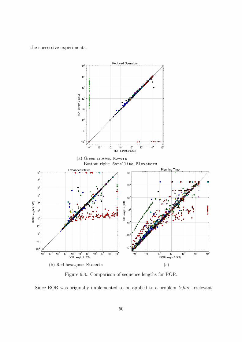
the successive experiments.
(a) Green crosses: RoversBottom right: Satellite, Elevators
(b) Red hexagons: Miconic (c)
Figure 6.3.: Comparison of sequence lengths for ROR.
Since ROR was originally implemented to be applied to a problem before irrelevant
50

and static variables are removed, one further experiment was conducted to see how ben-eficial it is to remove these variables before applying ROR. This was not considered forSafe Abstraction, as it is capable of abstracting irrelevant and static variables itself. Inthe case of Dominance Pruning, static variables are always removed before the pruningsince DP is implemented in the search component of Fast Downward.
(a) Red crosses: RoversGreen triangles: SatelliteGolden triangles: Trucks
(b)
Figure 6.4.: Comparison of ROR with and without previous static variable removal.
Instances solved aborted (time) aborted (memory) unsolvableBaseline 1406 401 71 8ROR 2 1368 411 99 8ROR 3 1382 418 78 8P+ROR 3 1397 410 71 8
Table 6.5.: Comparison of solved and aborted instances in different ROR configurationsout of 1886 total instances. ROR 2 uses an operator sequence limit of 2, P+ROR3 a limit of 3 and the removal of static variables.
Figure 6.4 shows the positive effect on reduced operators (a), together with a signif-icant benefit in runtime (b). The increased coverage is shown in Table 6.5, althoughhigher than in the previous experiments, it is still lower than the baseline coverage. An
51

(a) (b)
(c) (d)
Figure 6.5.: Redundant Operator Reduction (sequence limit 2, with static variable re-moval)
increased number of timeouts during the search is the cause of this, sometimes havingfewer redundant operators available actually slows down the search. Considering theobvious advantages of using static variable removal before ROR, it is performed in the
52
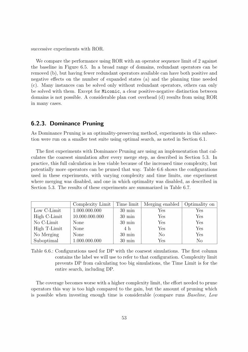
successive experiments with ROR.
We compare the performance using ROR with an operator sequence limit of 2 againstthe baseline in Figure 6.5. In a broad range of domains, redundant operators can beremoved (b), but having fewer redundant operators available can have both positive andnegative effects on the number of expanded states (a) and the planning time needed(c). Many instances can be solved only without redundant operators, others can onlybe solved with them. Except for Miconic, a clear positive-negative distinction betweendomains is not possible. A considerable plan cost overhead (d) results from using RORin many cases.
6.2.3. Dominance Pruning
As Dominance Pruning is an optimality-preserving method, experiments in this subsec-tion were run on a smaller test suite using optimal search, as noted in Section 6.1.
The first experiments with Dominance Pruning are using an implementation that cal-culates the coarsest simulation after every merge step, as described in Section 5.3. Inpractice, this full calculation is less viable because of the increased time complexity, butpotentially more operators can be pruned that way. Table 6.6 shows the configurationsused in these experiments, with varying complexity and time limits, one experimentwhere merging was disabled, and one in which optimality was disabled, as described inSection 5.3. The results of these experiments are summarized in Table 6.7.
Complexity Limit Time limit Merging enabled Optimality onLow C-Limit 1.000.000.000 30 min Yes YesHigh C-Limit 10.000.000.000 30 min Yes YesNo C-Limit None 30 min Yes YesHigh T-Limit None 4 h Yes YesNo Merging None 30 min No YesSuboptimal 1.000.000.000 30 min Yes No
Table 6.6.: Configurations used for DP with the coarsest simulations. The first columncontains the label we will use to refer to that configuration. Complexity limitprevents DP from calculating too big simulations, the Time Limit is for theentire search, including DP.
The coverage becomes worse with a higher complexity limit, the effort needed to pruneoperators this way is too high compared to the gain, but the amount of pruning whichis possible when investing enough time is considerable (compare runs Baseline, Low
53

Solved Prunable H1 H2 Operators PriceBaseline 820Low C-Limit 818 18.22% 85.94% 99.51% 40.18% 0%High C-Limit 624 59.62% 66.19% 96.79% 41.00% 0%No C-Limit 182 90.11% 69.78% 86.26% 52.45% 0%High T-Limit 204 91.18% 70.10% 87.25% 51.90% 0%No Merging 650 52.92% 34.29% 0%Suboptimal 816 19.00% 85.42% 99.51% 40.52% 1.06%
Table 6.7.: Coverage with different DP configurations, percentage of instances whichcontained at least one prunable operator, in which H1 and H2 hold. The lasttwo columns inform about how high the percentage of pruned operators andthe increase in plan costs is in average when the problem contains at leastone prunable operator.
C-Limit, High C-Limit, No C-Limit). The complexity of constantly recalculating thesimulation is so high that even a time limit of 4 hours (see run High T-Limit) hardlyincreased the coverage. Using the suboptimal approach did not result in a big change(compare runs Suboptimal with Low C-Limit), only in two domains, Scanalyzer andWoodworking, it made a small difference so that more operators could be pruned - ata small average plan cost increase of 1%, if pruning is possible. Since the increase inpruning using this modification is very limited, it is not used in the later experiments.When merging is disabled (see run No Merging), most of the instances in which pruningis possible are also pruned, though not as many operators can be removed as with en-abled merging. Two hypotheses were evaluated in these runs: The first one, H1, statesthat if operators can be pruned before merging, operators can also be pruned after merg-ing. The second one, H2, states that if no operators can be pruned before merging, nooperators can be pruned after merging. As the H1 results show, in general it does payoff to merge. The results of H2 show that the performance of DP before merging seemsto be a good indicator on whether it will be possible to prune after merging.
Table 6.8 shows the pruning that could be achieved in these runs in each domain.In some domains (Blocks, Gripper, Scanalyzer, Storage, Transport) no operatorscould be pruned without merging, while pruning was possible after merging, so for thesedomains merging seems to be vital to achieve any pruning. In reverse, merging did nothelp to find any more operators in the Movie domain.In a row of domains, pruning was not possible in any of the configurations used (Barman,Elevators, Freecell, Grid, Mprime, Openstacks, Parking, Pegsol, Pipesworld-tankage, Sokoban, Tidybot), though Kissmann and Torralba (2015) report possiblepruning in Elevators, Freecell and Sokoban. In general, there is no guarantee thatwith a longer run time no further operators could be pruned, though if an instance was
54

solved in a run without complexity limit, it has been completely merged, and pruningis definitely not possible there (such instances exist in Miconic, Openstacks, Tpp andVisitall). Compared to the results of Kissmann and Torralba (2015), by calculatingthe coarsest simulation often a much higher percentage of operators can be pruned, butthe time invested for that pruning is so high that only very few problems can be solvedbefore reaching a time limit.
Domain #Instances Low C-Limit High C-Limit No Merging No C-Limit High T-Limit Pi
Airport 50 0-78%, 2/25 3-85%, 11/11 3-13%, 13/13 32-85%, 6/6 32-85%, 6/6 13.00%Barman 20 0/4 0/4 0/4 0/0 0/0Blocks 35 0/28 0/28 0/28 31%, 3/3 31%, 3/3Depot 22 0/7 0/6 0/7 0/0 44%, 1/1Driverlog 20 0-5%, 4/14 1-41%, 13/13 1-8%, 13/13 41%, 1/1 41%, 1/1 1.00%Elevators 50 0/40 0/40 0/40 0/0 0/0 1 - 10%Floortile 20 0/7 28-29%, 9/9 28-29%, 9/9 0/0 29%, 2/2 2 - 28%Freecell 80 0/15 0/2 0/2 0/0 0/0 28.00%Grid 5 0/2 0/0 0/0 0/0 0/0Gripper 20 0/7 0-47%, 4/7 0/7 47-48%, 3/3 47-48%, 3/3 11.00%Logistics 63 0-85%, 10/26 26-85%, 27/27 20-47%, 27/27 59-85%, 7/7 58-85%, 10/10 42, 67%Miconic 150 0-45%, 30/141 0-45%, 88/93 11-45%, 90/95 0-45%, 20/25 0-45%, 24/29 58.00%Movie 30 74-96%, 30/30 74-96%, 30/30 74-96%, 30/30 74-96%, 30/30 74-96%, 30/30Mprime 35 0/22 0-1%, 1/6 0-1%, 1/6 0/0 0/0 0.00%Mystery 30 0-1%, 1/17 0-2%, 3/5 0-1%, 1/7 41%, 1/1 41%, 1/1 0.00%NoMystery 20 0/15 2-53%, 11/11 2-5%, 9/9 3-53%, 10/10 3-53%, 12/12 49.00%Openstacks 80 0/44 0/36 0/36 0/7 0/7 0.00%Parcprinter 50 0-59%, 6/34 28-67%, 39/39 11-63%, 11/11 28-57%, 12/12 28-61%, 16/16 38 - 77%Parking 20 0/3 0/0 0/0 0/0 0/0Pathways 30 0-60%, 4/5 47-73%, 5/5 47-60%, 5/5 59-73%, 2/2 59-73%, 2/2Pegsol 50 0/46 0/46 0/46 0/0 0/0 0.00%Pipesworld-not. 50 0/17 0-3%, 1/6 0/9 0/0 0/0 0.00%Pipesworld-t. 50 0/12 0/6 0/6 0/0 0/0 0.00%Psr-small 50 0-48%, 37/49 0-55%, 44/45 0-40%, 37/45 16-66%, 38/38 16-66%, 40/40 85.00%Rovers 40 0-48%, 7/9 14-53%, 9/9 14-50%, 9/9 35-53%, 4/4 35-53%, 4/4 71.00%Satellite 36 0-40%, 3/7 10-50%, 7/7 10-50%, 7/7 10-40%, 3/3 10-40%, 4/4 50.00%Scanalyzer 50 0/28 9-99%, 14/14 0/13 99%, 4/4 99%, 4/4 1, 0%Sokoban 50 0/50 0/27 0/42 0/0 0/0 8 - 9%Storage 30 0-63%, 2/15 0-68%, 6/15 0/15 1-72%, 4/4 41-72%, 4/4Tidybot 20 0/14 0/0 0/0 0/0 0/0Tpp 30 0-13%, 2/7 0-13%, 2/7 9-13%, 2/7 0/4 0/4 25.00%Transport 50 0/17 0/17 0/17 23-44%, 3/3 23-44%, 3/3 0.00%Trucks 30 0/10 67-87%, 7/7 67-87%, 7/7 73-79%, 2/2 73-79%, 2/2 90.00%Visitall 20 0-75%, 4/11 0-75%, 6/11 0-50%, 6/11 0-75%, 3/5 0-75%, 3/5 6.00%Woodworking 50 0-87%, 3/29 48-89%, 22/22 26-47%, 32/32 61-87%, 4/4 61-87%, 5/5 85 - 89%Zenotravel 20 0-58%, 4/13 42-58%, 13/13 42-53%, 13/13 55-58%, 4/4 55-58%, 4/4 43.00%
Table 6.8.: Domain-wise performance comparison of different DP configurations calcu-lating the coarsest simulations. The first and second value state the rangebetween minimum and maximum percentage of operators pruned per instancein that domain. The third value (behind the comma) states how many in-stances contained at least one prunable operator, out of the instances whichwere solved (4th value).The last column shows the average percentage of operators pruned in thePi configuration in Kissmann and Torralba (2015), which used incrementalcomputation and a time limit of 30 minutes.
55
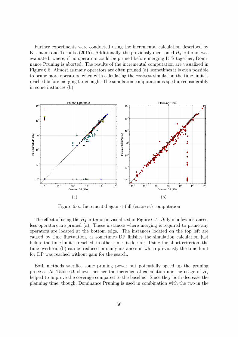
Further experiments were conducted using the incremental calculation described byKissmann and Torralba (2015). Additionally, the previously mentioned H2 criterion wasevaluated, where, if no operators could be pruned before merging LTS together, Domi-nance Pruning is aborted. The results of the incremental computation are visualized inFigure 6.6. Almost as many operators are often pruned (a), sometimes it is even possibleto prune more operators, when with calculating the coarsest simulation the time limit isreached before merging far enough. The simulation computation is sped up considerablyin some instances (b).
(a) (b)
Figure 6.6.: Incremental against full (coarsest) computation
The effect of using the H2 criterion is visualized in Figure 6.7. Only in a few instances,less operators are pruned (a). These instances where merging is required to prune anyoperators are located at the bottom edge. The instances located on the top left arecaused by time fluctuation, as sometimes DP finishes the simulation calculation justbefore the time limit is reached, in other times it doesn’t. Using the abort criterion, thetime overhead (b) can be reduced in many instances in which previously the time limitfor DP was reached without gain for the search.
Both methods sacrifice some pruning power but potentially speed up the pruningprocess. As Table 6.9 shows, neither the incremental calculation nor the usage of H2
helped to improve the coverage compared to the baseline. Since they both decrease theplanning time, though, Dominance Pruning is used in combination with the two in the
56

successive experiments.
(a) (b)
Figure 6.7.: Incremental Dominance Pruning using the H2 abort criterion.
Instances solved aborted (time) aborted (memory) unsolvableBaseline 820 627 2 7Full DP 818 628 3 7Incremental DP 818 630 1 7Incremental DP + H2 819 630 0 7
Table 6.9.: Coverage of different DP configurations compared to the baseline.
Figure 6.8 shows the results when comparing Dominance Pruning against the baseline.The number of expanded states (a) is considerably smaller, a few exceptions (above thediagonal) result from using the inconsistent LM-Cut heuristic. An increase in coverageis not achieved with DP, though, as even with the usage of the two previously describedmodifications, the time overhead (b) is immense - very often the time limit of 360seconds is reached. This conclusion matches the results described by Kissmann andTorralba (2015).
57

(a) (b)
Figure 6.8.: Performance of DP with H2 and incremental computation.
58

6.3. Pruning Power Synergies
In this section, we examine synergy effects by comparing the pruning power of eachtechnique on its own with the performance in combination with a different pruningmethod. In order to isolate the influence of synergies, each of the techniques in thissection receives a time limit of 180 seconds, meaning a combination of two techniqueshas a time limit of 360 seconds in total.
6.3.1. Safe Abstraction and Redundant Operator Reduction
As Figure 6.9 shows, positive synergies of SA+ROR, meaning that ROR can reduce moreoperators, occur only in Tpp and some Rovers instances. As Safe Abstraction nevercauses ROR to remove less operators, except for those which are already removed by SA(proven in Theorem 5), the number of search operators remaining in the problem is nevergreater when using the combination of both - though often less, when Safe Abstractionwas active enough (Satellite, Rovers, Logistics,..).
(a) Black triangles: TppGreen crosses: Rovers
(b) Bottom edge: Logistics, Miconic, MovieRed triangles: Satellite
Figure 6.9.: Synergies of using Safe Abstraction before ROR.
The reverse direction, ROR+SA, is visualized in Figure 6.10, although the positive syn-ergies are too small to be visible in the plot. In a large number of Woodworking, Pegsol,and Trucks instances, a small number of around 1-3 variables can be additionally ab-stracted when ROR has removed the redundant operators. Negative synergies do not
59
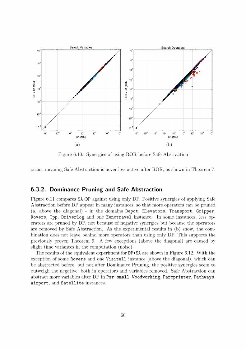
(a) (b)
Figure 6.10.: Synergies of using ROR before Safe Abstraction
occur, meaning Safe Abstraction is never less active after ROR, as shown in Theorem 7.
6.3.2. Dominance Pruning and Safe Abstraction
Figure 6.11 compares SA+DP against using only DP. Positive synergies of applying SafeAbstraction before DP appear in many instances, so that more operators can be pruned(a, above the diagonal) - in the domains Depot, Elevators, Transport, Gripper,Rovers, Tpp, Driverlog and one Zenotravel instance. In some instances, less op-erators are pruned by DP, not because of negative synergies but because the operatorsare removed by Safe Abstraction. As the experimental results in (b) show, the com-bination does not leave behind more operators than using only DP. This supports thepreviously proven Theorem 9. A few exceptions (above the diagonal) are caused byslight time variances in the computation (noise).
The results of the equivalent experiment for DP+SA are shown in Figure 6.12. With theexception of some Rovers and one Visitall instance (above the diagonal), which canbe abstracted before, but not after Dominance Pruning, the positive synergies seem tooutweigh the negative, both in operators and variables removed. Safe Abstraction canabstract more variables after DP in Psr-small, Woodworking, Parcprinter, Pathways,Airport, and Satellite instances.
60

(a) Bottom edge: Logistics, Miconic, Movie (b)
Figure 6.11.: Synergy effects of SA+DP.
(a) Green crosses: RoversBlue triangle: Visitall
(b)
Figure 6.12.: Synergy effects of DP+SA.
61
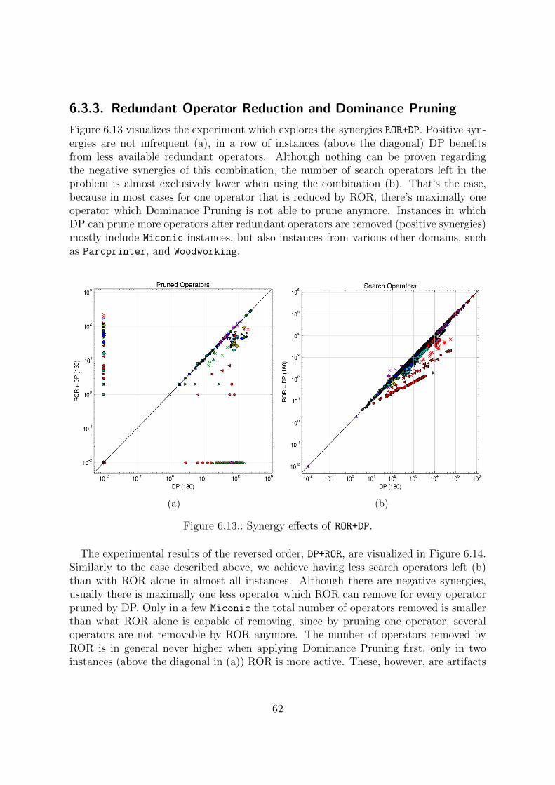
6.3.3. Redundant Operator Reduction and Dominance Pruning
Figure 6.13 visualizes the experiment which explores the synergies ROR+DP. Positive syn-ergies are not infrequent (a), in a row of instances (above the diagonal) DP benefitsfrom less available redundant operators. Although nothing can be proven regardingthe negative synergies of this combination, the number of search operators left in theproblem is almost exclusively lower when using the combination (b). That’s the case,because in most cases for one operator that is reduced by ROR, there’s maximally oneoperator which Dominance Pruning is not able to prune anymore. Instances in whichDP can prune more operators after redundant operators are removed (positive synergies)mostly include Miconic instances, but also instances from various other domains, suchas Parcprinter, and Woodworking.
(a) (b)
Figure 6.13.: Synergy effects of ROR+DP.
The experimental results of the reversed order, DP+ROR, are visualized in Figure 6.14.Similarly to the case described above, we achieve having less search operators left (b)than with ROR alone in almost all instances. Although there are negative synergies,usually there is maximally one less operator which ROR can remove for every operatorpruned by DP. Only in a few Miconic the total number of operators removed is smallerthan what ROR alone is capable of removing, since by pruning one operator, severaloperators are not removable by ROR anymore. The number of operators removed byROR is in general never higher when applying Dominance Pruning first, only in twoinstances (above the diagonal in (a)) ROR is more active. These, however, are artifacts
62

of a different variable ordering: Dominance Pruning did not remove any operator fromthe tasks. As shown in Theorem 14, positive synergies would be possible, but only inrare cases - since a variable needs to become static, which then has to cause an operatorto become redundant - this did not appear in any domain.
(a) (b)
Figure 6.14.: Synergy effects of DP+ROR.
63
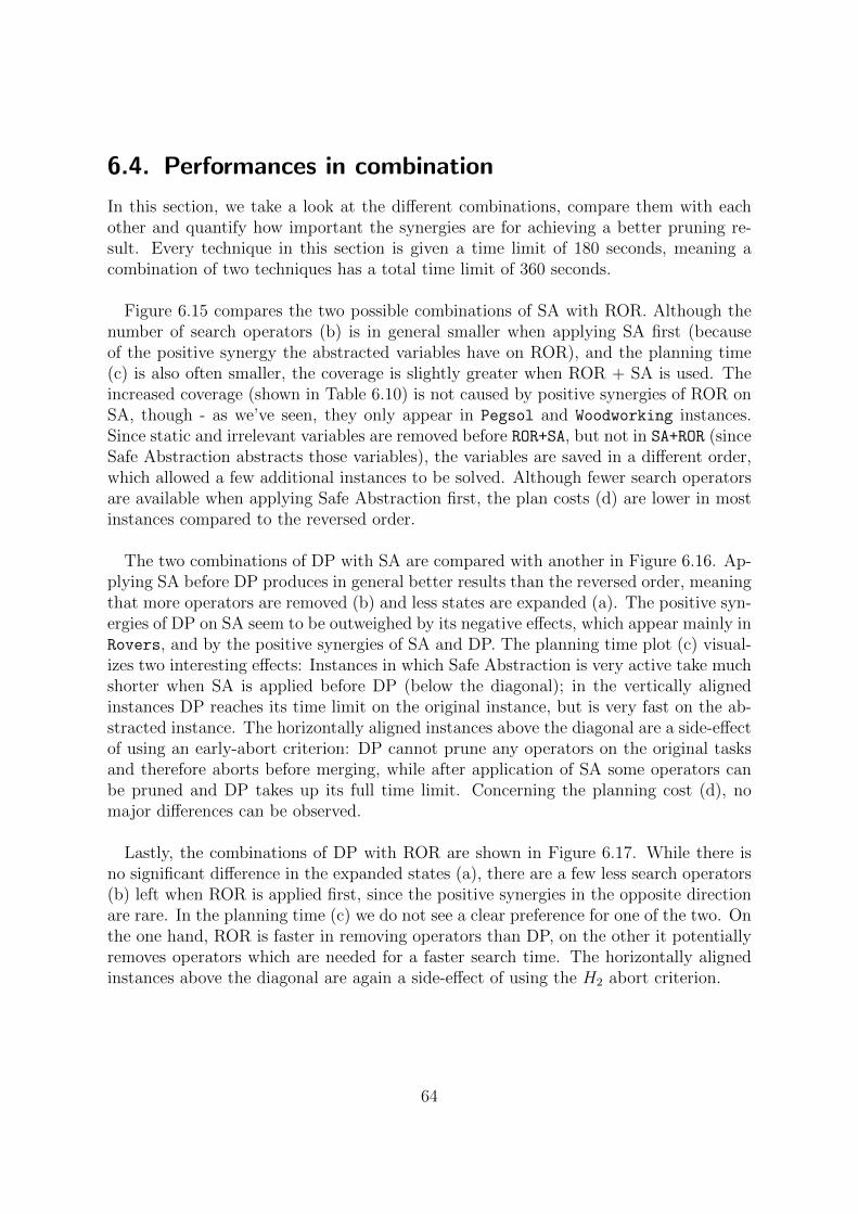
6.4. Performances in combination
In this section, we take a look at the different combinations, compare them with eachother and quantify how important the synergies are for achieving a better pruning re-sult. Every technique in this section is given a time limit of 180 seconds, meaning acombination of two techniques has a total time limit of 360 seconds.
Figure 6.15 compares the two possible combinations of SA with ROR. Although thenumber of search operators (b) is in general smaller when applying SA first (becauseof the positive synergy the abstracted variables have on ROR), and the planning time(c) is also often smaller, the coverage is slightly greater when ROR + SA is used. Theincreased coverage (shown in Table 6.10) is not caused by positive synergies of ROR onSA, though - as we’ve seen, they only appear in Pegsol and Woodworking instances.Since static and irrelevant variables are removed before ROR+SA, but not in SA+ROR (sinceSafe Abstraction abstracts those variables), the variables are saved in a different order,which allowed a few additional instances to be solved. Although fewer search operatorsare available when applying Safe Abstraction first, the plan costs (d) are lower in mostinstances compared to the reversed order.
The two combinations of DP with SA are compared with another in Figure 6.16. Ap-plying SA before DP produces in general better results than the reversed order, meaningthat more operators are removed (b) and less states are expanded (a). The positive syn-ergies of DP on SA seem to be outweighed by its negative effects, which appear mainly inRovers, and by the positive synergies of SA and DP. The planning time plot (c) visual-izes two interesting effects: Instances in which Safe Abstraction is very active take muchshorter when SA is applied before DP (below the diagonal); in the vertically alignedinstances DP reaches its time limit on the original instance, but is very fast on the ab-stracted instance. The horizontally aligned instances above the diagonal are a side-effectof using an early-abort criterion: DP cannot prune any operators on the original tasksand therefore aborts before merging, while after application of SA some operators canbe pruned and DP takes up its full time limit. Concerning the planning cost (d), nomajor differences can be observed.
Lastly, the combinations of DP with ROR are shown in Figure 6.17. While there isno significant difference in the expanded states (a), there are a few less search operators(b) left when ROR is applied first, since the positive synergies in the opposite directionare rare. In the planning time (c) we do not see a clear preference for one of the two. Onthe one hand, ROR is faster in removing operators than DP, on the other it potentiallyremoves operators which are needed for a faster search time. The horizontally alignedinstances above the diagonal are again a side-effect of using the H2 abort criterion.
64
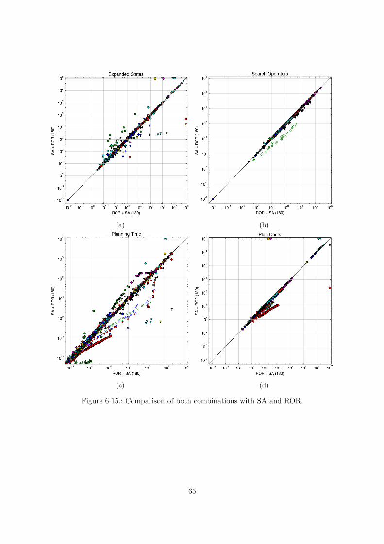
(a) (b)
(c) (d)
Figure 6.15.: Comparison of both combinations with SA and ROR.
65

(a) (b) Green crosses: Rovers
(c) (d)
Figure 6.16.: Comparison of both combinations with DP and SA.
66
(a) (b)
(c) (d)
Figure 6.17.: Comparison of both combinations with DP and ROR.
67
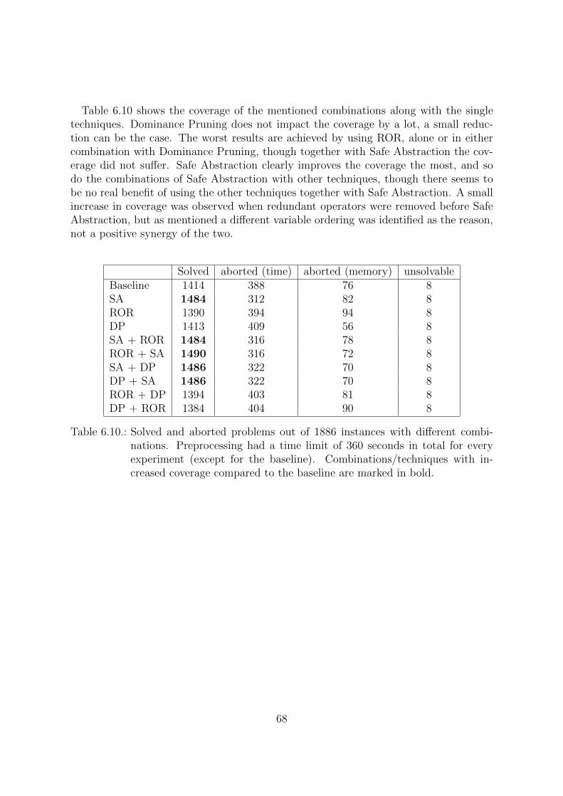
Table 6.10 shows the coverage of the mentioned combinations along with the singletechniques. Dominance Pruning does not impact the coverage by a lot, a small reduc-tion can be the case. The worst results are achieved by using ROR, alone or in eithercombination with Dominance Pruning, though together with Safe Abstraction the cov-erage did not suffer. Safe Abstraction clearly improves the coverage the most, and sodo the combinations of Safe Abstraction with other techniques, though there seems tobe no real benefit of using the other techniques together with Safe Abstraction. A smallincrease in coverage was observed when redundant operators were removed before SafeAbstraction, but as mentioned a different variable ordering was identified as the reason,not a positive synergy of the two.
Solved aborted (time) aborted (memory) unsolvableBaseline 1414 388 76 8SA 1484 312 82 8ROR 1390 394 94 8DP 1413 409 56 8SA + ROR 1484 316 78 8ROR + SA 1490 316 72 8SA + DP 1486 322 70 8DP + SA 1486 322 70 8ROR + DP 1394 403 81 8DP + ROR 1384 404 90 8
Table 6.10.: Solved and aborted problems out of 1886 instances with different combi-nations. Preprocessing had a time limit of 360 seconds in total for everyexperiment (except for the baseline). Combinations/techniques with in-creased coverage compared to the baseline are marked in bold.
68

6.5. Unsolvable instances
In this section, we evaluate the three pruning techniques on a set of problem domainsin which all instances are unsolvable. We use the unsolvable benchmarks by Hoffmannet al. (2014) as well as unsolvable benchmarks by Jendrik Seipp, Florian Pommerening,Chris Fawcett, Silvan Sievers, Yusra Alkhazraji and Martin Wehrle (the latter bench-marks have been generated in the context of their portfolio planner submission to theunsolvability IPC 2016).
The aim of a planner in such an instance is to prove that it is unsolvable, for whichevery state in the state space needs to be expanded. Since all three pruning techniquesare solution-preserving, proving that the pruned problem is unsolvable is sufficient toprove the same for the original problem.
Figure 6.18 shows the expanded states and the planning time when using Safe Ab-straction against a run without it (both with greedy search and FF heuristic). Thedomains represented by the symbols are listed in Figure 6.19.
(a) (b)
Figure 6.18.: Performance of Safe Abstraction on unsolvable problem instances.
The advantage of Safe Abstraction in this context is that refining a plan is not neces-sary, since no plan exists. We can see that in a row of domains Safe Abstraction reducesthe number of states in the search space considerably (a), while in other domains it hasno effect at all. Similarly, the planning time (b) needed to prove that a problem is un-solvable is reduced for the same instances, it also completes expanding the search space
69

Figure 6.19.: Legend for the plots in Figure 6.18.
in some instances where without Safe Abstraction the time limit is reached. (instanceson the right edge).
As every state in the search space needs to be expanded, Redundant Operator Reduc-tion does not have any benefit since it does not prune any state. Dominance Pruningallows to prune less states only in a small number of instances and at the same timeintroduces a huge overhead in time for the computation, so often the search space cannotbe completely expanded anymore. Both these techniques do not seem to be well suitedto be used in the context of unsolvable instances.
70
7. Discussion on Safe Abstraction
As the experiments in the previous chapter have shown, despite the existing positivesynergies between the pruning techniques, applying two of them in combination doesnot yield a better coverage than either of the techniques does separately (when exclud-ing noise effects). Safe Abstraction is responsible for the improved coverage in each ofits combinations, and it also causes that increase on its own. Being the most promisingof the three techniques, we discuss one possible extension to Safe Abstraction in thischapter. This extension has not been implemented in this work, we describe the generalidea and the conditions for Safe Abstraction in an informal way.
Although the conditions for Safe Abstraction are defined on the domain transitiongraphs of variables, they could as well be defined on the atomic transition systems, sinceboth contain the relevant information. The states in the ATS are then the equivalent ofthe values of the variable. One extension that could possibly improve the power of SafeAbstraction further is to merge these transition systems together and to compute SafeAbstractions on the so-achieved LTSs, abstracting several variables together which arenot safe on their own, but whose merged transition system is safe. An example of suchan instance is shown in Figure 7.1.
After merging and abstracting (v1, v2) together, v3 also becomes safe, and a search isnot needed therefore. Refining that plan would first form a less abstract task by rein-serting v3, for which 〈x〉 is a plan. Then (v1, v2) would be reinserted. For the operatorx in the abstract plan, a path must be found in the merged LTS from the initial stateI1I2 to R1R2, as x has that requirement. Either 〈e, f1, f2, x〉 or 〈e, f2, f1, x〉 are plansthat would be created by the refinement process.In the extreme case in which all LTS are merged together, no operator has any condi-tion/effect on an external variable, meaning the only condition for Safe Abstraction isthat a goal state is reachable from the initial state. All variables are safely abstractabletogether if a plan exists. However, there is no benefit in merging up to that point, asthe entire effort of the search would be moved to the refinement process, in which a pathfrom the initial state to a goal state needs to be found. Considering that there is theadditional overhead of finding out whether a path exists, to fulfill the conditions for SafeAbstraction, the work would be doubled compared to a simple search. Clearly a mea-surement needs to be found to determine at which point this strategy is not beneficialanymore.
The example shown in Figure 7.1 is too small, so that any abstraction slows down
71

I1start
I2start
I3start
T R1
R2
G
v1
v2
v3
e f1
f2
x
f2 f2 f2, x
e, f1 f1, x
f1, f2, e f1, f2, e
(a) ATS of three variables v1, v2, v3. Novariable is safe, as R1 / I2 / G are notfree reachable from I1 / R2 / I3.
I1I2start I1R2
TI2 TR2
R1I2 R1R2
f2
e
f2
f1
f2
f1
x
(b) LTS of v1 ⊗ v2. Safely ab-stractable, as e, f1 and f2 have noeffect/condition on the third vari-able.
Figure 7.1.: Problem instance (with variables v1, v2, v3) in which Safe Abstraction wouldbe possible on merged transition systems. Externally required values aremarked in red. The dotted edges correspond to operators which have noeffect on that variable.
the search. The state space of the original problem that needs to be searched contains7 reachable states, including the initial state. Abstracting (v1, v2) means that the re-maining abstract problem contains 2 states (those of v3) that need to be searched. Forthe refinement, the merged LTS needs to be searched for a path, containing 6 reach-able states. With the additional overhead for abstraction (merging the LTS, detectionwhether it’s safe, building the abstract problem) there cannot be any gain.In general, when abstracting an LTS with n states, the abstracted problem’s searchspace (including unreachable states) has n times fewer states. The costs of this oper-ation are the reachability checks for abstraction and shortest-path searches (both onthose n states) for every operator that needs to be inserted into the plan. If the totalnumber of states in the search space is considerably larger than n, then abstracting theLTS should prove to be useful.
To abstract several variables together, the conditions for safe variables need to be
72

reconsidered. In the above example, it is obvious that the state R1R2 is externallyrequired, since it is the only state in which the operator x is applicable. If the operatorwas applicable in several states, though, meaning it had a precondition on only one of thevariables, defining all of them to be externally required states would be very restrictive.The same applies to goal states, if only one of the two variables has a goal value, andto externally caused states. If all of these states have to be connected according toHaslum’s condition, not many additional variables can be abstracted in this way. Outof the domains examined in this work, there’s only one instance in which two variablesexist which are not safe on their own, but could be abstracted using this concept. Thatinstance from the Zenotravel domain is shown in Figure 7.2.
In this Zenotravel instance, a plane can travel (fly) between 3 cities, c0, c1 and c2 (b).Two passengers (a, c) can board the plane when the plane is located at their startingcity, and debark the plane later on again. Every flight costs the plane one level of fuel(d), it can be refueled at any city. The goal is for the passengers to arrive at their desti-nation, and for the plane to arrive at the city c1. A plan for this problem is 〈flyc0−→c1,f1〉,since the passenger are already at their destination in the initial state.
The two variables encoding the passenger’s location (a, c) are both safe: Neither ofthem has an externally required value, and their initial state is equal to their goal state.The two variables encoding the plane’s location and its level of fuel cannot be abstracted,since the fly and refuel operators have preconditions and effects on both of them. Merg-ing the two ATS together, every state c∗f∗ in the resulting LTS is free reachable fromany other state. Therefore, abstracting those two variables together is possible. Sinceno variables are left in the abstract problem, no search is needed. To refine the plan, apath must be found in the merged LTS from the state c0f1 to any goal state c1f∗, eitherby directly flying from c0 to c1, or by first refueling or making a detour to c2.
Requiring free reachability of all states, in which operators are applicable that workon other variables, appears to be too restricting. The concept behind safe variablesis, that every abstract plan can be refined to a plan for the concrete problem. Thisrefining is still possible when not all relevant states are freely reachable, but it requiresa more complex refining algorithm. Consider Figure 7.3 for an example, which depictsa problem instance with three variables. None of the variables is initially safe: In v1,the externally required value R1 is not free reachable from the initial state. In v2, theexternally required value I is not free reachable from R2. In v3, the goal value is notfree reachable from the initial state.Subfigure (b) shows the LTS resulting from merging the ATS of v1 and v2 together.Using the strict condition mentioned above, the two variables are not safely abstractable,since some externally required values are not free reachable from IR2. However, if thevariables were abstracted, every plan for the resulting abstract problem could be refinedto a concrete plan, as long as the refining algorithm ensures that the state IR2 is notreached, since from that state, no other state is free reachable in which y is applicable.
73

c0start
plane
c1c2
boardp1,c0
boardp1,c1
boardp1,c2
debarkp1,c0
debarkp1,c1
debarkp1,c2
(a) ATS of the variable encoding the loca-tion of passenger 1. The refuel ..., fly...,boardp2,∗ and debarkp2,∗ transitions are notdepicted and applicable in every state.
c0start
c2c1
flyc0−→c1,f∗
flyc1−→c2,f∗
flyc2−→c0,f∗
debarkp∗,c0 , boardp∗,c0 , refuel...,c0
. . .. . .
(b) ATS of the variable encoding theplane’s location. A flya−→b,f∗ edgein the graph represents one transitionfrom a to b for every possible level offuel.
c0
plane
c1c2start
boardp2,c0
boardp2,c1
boardp2,c2
debarkp2,c0
debarkp2,c1
debarkp2,c2
(c) ATS of the variable encoding the location ofpassenger 2. The refuel..., fly..., boardp1,∗ anddebarkp1,∗ transitions are not depicted and ap-plicable in every state.
f0 f1start f2 f3 f4
refuelf0−→f1,c∗ refuelf1−→f2,c∗ refuelf2−→f3,c∗ refuelf3−→f4,c∗
flyc∗−→c∗,f1 flyc∗−→c∗,f2 flyc∗−→c∗,f3 flyc∗−→c∗,f4
(d) ATS of the variable encoding the level of fuel. A flyc∗−→c∗,fa edge in the graphrepresents one transition for every two cities, refuelfa−→fb,c∗ equivalently. TheThe board... and debark... transitions are not depicted and applicable in everystate.
Figure 7.2.: Zenotravel instance in which a merged LTS allows the safe abstraction oftwo variables
74

v1
v2
v3
Istart
Istart
Istart
T
R2
T
R1
G
e f1y
e
f2x
x y
(a) ATS of the three variables v1, v2, v3. Thetransitions of f1, f2 and e are not depictedin the LTS in which they do not have aprecondition or an effect.
v1 ⊗ v2
IIstart
IR2
TI
TR2 R1R2
R1Ie f1
f2 f2
f1
f2
y
x x x
y
(b) ATS of v1 and v2 merged together.
Figure 7.3.: Example instance with three variables, in which merging and abstracting v1and v2 requires a different refining algorithm.
Removing v1 and v2, the abstract plan is 〈x, y〉. When refining, the preconditions of xon v2 need to be satisfied first. A naive refining algorithm might apply f2 directly, sincethen the preconditions are satisfied. Since IR2 must not be visited, either the state TR2
or R1R2 can be considered.To ensure that every abstract plan can be refined, a definition of Safe Abstraction on
merged LTS needs to contain an at least one-semantic. For every externally requiredvalue of one variable, at least one state sr in the merged LTS assigning that value must befree reachable from at least one state for every other externally required value and fromthe initial state. If externally caused values exist, sr must also be free reachable from atleast one state sc for each externally caused value. Further, denoting the operator whichcauses that externally caused value with o, we need to ensure that one state so mustbe free reachable, in which a transition so
o−→ sc exists. Otherwise, if the operator o isapplied in the abstract plan, it might not be possible for the refining algorithm to endup in sc after o is applied but in some other state caused by the operator, from whichthe externally required states are not free reachable.In summary, a cluster of states must exist in the merged LTS which allows every operatorto be applied and every goal condition to be satisfied. The refining algorithm must thenensure that while inserting operators into the abstract plan, it never runs into a deadend (like the state IR2 in Figure 7.3.b).
75

8. Conclusion
To conclude, we first briefly review the subjects covered in this work and then recapit-ulate the results of the thesis in more detail.
In this work, we have discussed three different existing static pruning techniques, SafeAbstraction, Redundant Operator Reduction, and Dominance Pruning. We analysedhow each of them prunes the search space, and proposed modifications and extensionsto them in order to further increase their pruning power. We investigated the possiblesynergy effects in each combination of two pruning methods, and observed that most ofthe synergies also occur in instances of IPC benchmarks. We described the implemen-tation of the three techniques into an existing propositional planner and evaluated themethods on IPC benchmarks. We measured the performance of different configurationsfor each technique, and the magnitude of the synergy effects between the methods.
As two conditions for Safe Abstraction have been proposed, we have compared theirperformances with each other. Both lead to a considerable increase of coverage, Haslum’scondition allows to abstract more variables in many domains and to solve some addi-tional domains without search. When used in the context of unsolvable instances, SafeAbstraction reduces the number of states which need to be expanded, consequentlyspeeding up the search process. To further extend this technique, we discussed an ideain the last chapter based on calculating Safe Abstractions on merged atomic transitionsystems. This approach has not been implemented yet, but is an interesting point forfuture research.
The technique of Redundant Operator Reduction has so far only been used on a smallset of domains. In this work, we have evaluated it on a bigger set. Although ROR iscapable of removing many operators from the planning tasks, its pruning is not consis-tently beneficial for the search. In many instances, having fewer redundant operatorsavailable leads to an increase in the number of states which have to be expanded andin the search time. A dynamic version of ROR, which avoids to prune transitions basedon knowledge used in Tunnel Macros, might be able to reduce these negative effects.
We observed that ROR can be combined together with Safe Abstraction without ei-ther of the techniques having negative effects on the pruning power of the other. Whilepositive synergies do exist, they are too weak to increase the coverage.
As a third pruning method, we have studied the static version of Dominance Pruning.
76
We proposed an implementation that allows to prune transitions which subsume eachother in order to increase the number of operators that can be removed. The techniqueis able to remove many operators, consequently fewer states need to be expanded, butthe preprocessing overhead does not pay off in terms of overall planning time, even whenusing the incremental computation and an early-abort criterion. If Dominance Pruningis allowed to ignore label costs, only very few operators can be pruned additionally.
Despite being an optimality-preserving method, we were able to identify positive syn-ergy effects on Dominance Pruning when the two satisficing techniques are used beforeit. In practice, the methods would not be combined because the optimality-preservingproperty is lost, and the overhead of DP is too high as a satisficing preprocessing method.If a faster, suboptimal variant of DP was found, it could be used for satisficing searchin combination with Safe Abstraction.
77

A. Plot legend
78

B. Bibliography
Alkhazraji, Y., Wehrle, M., Mattmuller, R., and Helmert, M. (2012). A stubborn setalgorithm for optimal planning. Proc. 20th European Conference on Artificial Intelli-gence (ECAI 2012), pages 891 – 892.
Backstrom, C. and Nebel, B. (1995). Complexity results for SAS+ planning. Computa-tional Intelligence, 11(4):625 – 655.
Crawford, J., Ginzberg, M., Luks, E., and Roy, A. (1996). Symmetry-breaking predicatesfor search problems. KR, 96:148 – 159.
Dijkstra, E. W. (1959). A note on two problems in connexion with graphs. NumerischeMathematik, 1:1:269 – 271.
Domshlak, C., Katz, M., and Shleyfman, A. (2012). Enhanced symmetry breaking incost-optimal planning as forward search. Proc. ICAPS 2012.
Domshlak, C., Katz, M., and Shleyfman, A. (2013). Symmetry breaking: Satisficingplanning and landmark heuristics. Proc. ICAPS 2013, pages 298 – 302.
Fox, M. and Long, D. (1999). The detection and exploitation of symmetry in planningproblems. Proc. 16th International Joint Conference on Artificial Intelligence (IJCAI-99), pages 956 – 961.
Godefroid, P. (1996). Partial-order methods for the verification of concurrent systems -an approach to the state-explosion problem. Springer-Verlag, 1032 of LNCS.
Hart, P. E.; Nilsson, N. J. and Raphael, B. (1968). A formal basis for the heuristicdetermination of minimum cost paths. IEEE Transactions on Systems Science andCybernetics, 4(2):100 – 107.
Haslum, P. (2007). Reducing accidental complexity in planning problems. Proc. 20thInternational Joint Conference on Artificial Intelligence (ICJAI-07), pages 1898 –1903.
Haslum, P., Botea, A., Helmert, M., Bonet, B., and Koenig, S. (2007). Domain-independent construction of pattern database heuristics for cost-optimal planning.Proc. AAAI 2007, pages 1007 – 1012.
79

Haslum, P. and Jonsson, P. (2000). Planning with reduced operator sets. Proc. 5thInternational Conference on Artificial Intelligence Planning and Scheduling (AIPS2000), pages 150 – 158.
Helmert, M. (2006). Fast (diagonally) downward. 5th International Planning Competi-tion Booklet. Available at: http://zeus.ing.unibs.it/ipc-5/ (Accessed: 2016-05-06).
Helmert, M. and Domshlak, C. (2009). Landmarks, critical paths and abstractions:What’s the difference anyway? Proc. 19th International Conference on AutomatedPlanning and Scheduling (ICAPS 2009), pages 162–169.
Helmert, M. and Geffner, H. (2008). Unifying the causal graph and additive heuristics.Proc. 18th International Conference on Automated Planning and Scheduling (ICAPS2008), pages 544 – 550.
Hoffmann, J., Kissmann, P., and Torralba, A. (2014). ”distance”? who cares? tailoringmerge-and-shrink heuristics to detect unsolvability. Proc. 21st European Conferenceon Artificial Intelligence (ECAI 14), pages 441 – 446.
Hoffmann, J. and Nebel, B. (2001). The FF planning system: Fast plan generationthrough heuristic search. Journal of Artificial Intelligence Research, pages 253 – 302.
Holte, R. C., Alkhazraji, Y., and Wehrle, M. (2015). A generalization of sleep setsbased on operator sequence redundancy. Proc. 29th AAAI Conference on ArtificialIntelligence (AAAI 2015), pages 3291 – 3297.
Junghanns, A. and Schaeffer, J. (2001). Sokoban: Enhancing general single-agent searchmethods using domain knowledge. Artificial Intelligence, 129:219 – 251.
Kissmann, P. and Torralba, A. (2015). Focusing on what really matters: Irrelevancepruning in merge-and-shrink. Proc. 8th International Symposium on CombinatorialSearch, pages 122 – 130.
Nissim, R., Apsel, U., and Brafman, R. (2012). Tunneling and decomposition-basedstate reduction for optimal planning. ECAI, pages 624 – 629.
Pochter, N., Zohar, A., and Rosenschein, J. S. (2011). Exploiting problem symmetriesin state-based planners. Proc. AAAI 2011, pages 1004 – 1009.
Pommerening, F., Roger, G., Helmert, M., and Bonet, B. (2014). LP-based heuristics forcost-optimal planning. Proc. 24th International Conference on Automated Planningand Scheduling (ICAPS 2014), pages 226 – 234.
Sievers, S., Wehrle, M., and Helmert, M. (2014). Generalized label reduction for merge-and-shrink heuristics. Proc. 28th AAAI Conference on Artificial Intelligence (AAAI2014), pages 2358 – 2366.
80

Tarjan, R. (1972). Depth-first search and linear graph algorithms. SIAM Journal onComputing, 1(2):146 – 160.
Torralba, A. and Hoffmann, J. (2015). Simulation-based admissible dominance pruning.Proc. 24th International Joint Conference on Artificial Intelligence (IJCAI’15).
Valmari, A. (1989). Stubborn sets for reduced state space generation. Proc. 10th Inter-national Conference on Applications and Theory of Petri Nets (APN 1989), pages 1– 22.
Wehrle, M. and Helmert, M. (2009). The causal graph revisited for directed modelchecking. Proc. 16th International Static Analysis Symposium (SAS 2009), pages 86– 101.
Wehrle, M. and Helmert, M. (2012). About partial order reduction in planning andcomputer aided verification. Proc. 22th ICAPS 2012, pages 297 – 305.
Wehrle, M. and Helmert, M. (2014). Efficient stubborn sets: Generalized algorithmsand selection strategies. Proc. 24th ICAPS 2014, pages 323 – 331.
81