XLV Reunión AnualNoviembre de 2010

ISSN 1852-0022ISBN 978-987-99570-8-0

SPECTRAL ANALYSIS OF THE BEHAVIOUR OF THE INDEX OF ECONOMIC ACTIVITY IN ARGEENTINA 1993-2009

Baccino, Osvaldo

ANALES | ASOCIACION ARGENTINA DE ECONOMIA POLITICA

Spectral Analysis of the Behaviour of the Index of Economic Activity in Argentina 1993-2009

by Osvaldo E. Baccino 1. Introduction The aim of this paper is to inquire into the inner dynamic behaviour of the official indicator of economic activity (EMAE) elaborated by the National Institute of Statistics and Census of Argentina (INDEC). The analysis develops on the frequency domain approach to time series. In other words, this entails the spectral decomposition of the data into several oscillations of major frequencies explaining variances in an observed time series and modelling those components. The idea is to study the components of dynamic behaviour particularly those aspects, which look permanent in the series. In particular, it seems that at least, since the beginnings of 1993 until the end of 2009, there are two very different segments denoting drastic changes. At first sight, the dividing line occurs in the early 2002. The present work attempts to identify the conditions of such a break in the behaviour of the series. Given that many doubts arose about the reliability of certain official indicators both in inner and external circles, it is important to analyse the hidden structure of the EMAE to explain the relationships between different components. These doubts emerged in the course of a slow process that started after 2002. The monthly estimate of economic activity published by the INDEC is one of the indexes that called for the attention. This indicator is very important, because it is closely related to the construction of the Quarterly Gross Domestic Product series elaborated by the area of National Accounts of the Ministry of the Economy. 2. The area of study The monthly indicator of Economic Activity (1993 =100) measures the level of economic activity at prices of 1993. INDEC publishes EMAE in three versions: an original series, a seasonally adjusted series and a smoothed trend series. The latter evolves in very similar way to a Hodrick-Prescott filtered series. Unfortunately, INDEC does not publish a disaggregate version of the Monthly Economic Activity Indicator and this sets a limit to the economic analysis of the cyclicity of the series. The present analysis uses the original data of EMAE (see Annex 1) in order to capture all types of variations of the Indicator. The index of economic activity presented in figure 1 shows two different kinds of performance. The first segment runs from January 1993 until January 2002 and it describe the usual evolution in the past. The other segment with different performance corresponds to the rest of the series up to December 2009. At first sight, the periodic variations repeat themselves with remarkable regularity while, on the contrary, there is a sharp change in the trend movements between both sections of the sample. However, the inner structure of the time series might undergo modifications, which are not easily seen with a naked eye.

2

8010

012

014

016

018

0em

ae

1992m11994m11996m11998m12000m12002m12004m12006m12008m12010m1period

Monthly Economic Activity Indicator (EMAE)

Fig. 1.a

In figure 1.a, there appear two different kinds of trend. From the beginning of the series up to January 2002, the trend follows a non-linear evolution. Firstly, it has an upswing until the start of 1999. Then a downswing follows that prevails until the end of the first section in January 2002. Later, the trend suddenly changes and undergoes a continuous rise at a constant rate up to the end of 2009.

9.2

40

-4-1

0.9

Gro

wth

%

1995 2000 2005 2010Yeat

Rates of GrowthGross Domestic Product at 1993 prices

Fig. 1.b

This behaviour is reflected in the annual change of the GDP at constant prices in the figure 1.b. The annual rates of growth of GDP equal the annual rates of growth of EMAE.

3

Perhaps, the high rates of growth of the economic activity in real terms make the evolution of the index incredible. This type of long run behaviour is rather curious particularly for its permanence through time. It depicts an economy growing at a very high steady rate of growth while the general conditions for a boom of such importance do not seem to be present in the economy at the time. Therefore, the present study will focus on some components of the series such as trend, deterministic cycles and stationary stochastic process. The aim is to relate the analysis of periodic movements both deterministic and stochastic with the characteristics of the trend. 3. The method The analysis starts from the detection of the hidden waves as peak frequencies in the spectral density function associated with the time series under study. The identification of the kinds of cycles precedes the specification of a model that decomposes the series into trend, deterministic cycles, stochastic cycles, and white noise. A basic instrument in the first stage is the raw periodogram as a measure of the function of spectral density. This device measures the part of the total variance of the series corresponding to given frequencies. Frequency means how things repeat themselves and is measured in cycles per unit of time. For the sake of simplicity, the raw periodogram is used instead of a smoothed version of it.. In this paper the computation of Schuster’s periodogram uses the following formula:

+

= ∑∑−

=

−

=

21

0

21

0

22cos2

1)(

T

tt

T

tt ftsenxftx

TfI ππ

π (1)

where I(f) is the ordinate value of the density function for a given frequency f, xt is the value of variable under analysis in time t; T is the number of observations in the sample and t is the variable time. The null hypothesis says that the regression coefficients of the fitted cyclical performance at a given f are A1=A2= 0. Thus the periodogram ordinate test is I(f) ~ (σ2/2π) (χ2 / 2) chi2(2)/2 can be tested with F(2, ∞ ) The periodogram allows finding out the relevant frequencies of deterministic cycles The model of cyclicities of a given time series is given by the discrete Fourier transform1

1 Bloomfield, P. (2000). The time series is expressed as the sum of sine waves at the Fourier’s frequencies.

4

{ }tffAtffBtffAAx Tjjjjj

Tj

t 2/

2/0

2cos)(2sin)(2cos)(2)0( ][ πππ +

Σ+= +<<

(2) The summation is over the frequencies fj = j/T. The last term in braces is only incorporated when T is even. t = 0, 1, 2, …, T-1. A particular cycle fitting is obtained by the regression

xcycle j = A1 sin(2πfj t) + A2 cos(2πfj t) + εt (3)

for a given frequency fj (equal to the inverse of the cycle length). εt is a disturbance term with mean zero and variance σ2. The regression coefficients A1’s correspond to the B’s, and the A2’s to A’s of equation (2). This fitting is equivalent to a sin wave of the form yt = A sin(ws t + φ) (4) where ws is the angular frequency, which measures the number of complete cycles in 2π units of time; Coefficient A is the amplitude that represents the magnitude of the change from maximum to minimum of the cycle. Finally, φ is the initial phase that means a shift in the sine wave. The values of A and φ can be computed from the regression coefficients A1 and A2 by the application of trigonometric identities. The original series must be transformed into a nonstationary series by differencing or by removing a trend before computing the periodogram. Then this instrument is helpful to identify the hidden structure of periodic oscillations. Now, it follows the removal of the deterministic cycles from the series, so that the residual includes the probabilistic cycles. This component is fitted by an ARMA(p,q) model leaving a residual as white noise. So that, the model can detect each main component of the series and so it provides the basis of comparison for several subsets of the original data. Since the study concerns the treatment of two important sections of the data where the main differences deal with sharp changes in trend, it means that low frequencies will be important in the following comparisons. Therefore, the more adequate transformation of the original data to render a stationary time series is the removal of a linear trend instead of differencing the series. Yt = original data Ψt = linear trend Original data de-trended Xdt = Yt - Ψt Differenced original data ∆Yt = Yt - Yt-1

5

∆ Xdt = (Yt - Ψt) - (Yt-1 - Ψt-1) = (Yt - Yt-1) - (Ψt - Ψt-1) Then, (Yt - Yt-1) = ∆ Xdt + (Ψt - Ψt-1) (5) Equality (5) expresses the relationship between the differenced and de-trended versions of original data. If the trend is linear the term between brackets on the right side is a constant. Therefore, the choice was adopting the removal of a linear trend. The residual means the level of the variable minus the trend. This procedure allows the inclusion of certain low frequency oscillations which makes the analysis more interesting, particularly when appraising the section of high steady growth in EMAE series. 4. Detection of cyclicities in four different kinds of samples The examination of the hidden structure of oscillations of the series goes on in three samples or segments of the EMAE series

(a) Analysis of two samples of equal size two realizations of the time series. Both samples have in common a subset of observations. The EMAE was split in two samples of 158 monthly observations each. Sample 1 covers the period Jan1993- Feb 2006.2 Sample 2 includes data from Nov 1996 to Dec 2010. The comparison of two samples of equal size aimed at detecting permanent characteristics of the dynamic behaviour of the EMAE.

(b) Analysis of the period running from Feb 2002 to Dec2009. This section of the data (sample 3) includes some peculiar changes in the behaviour of the indicator. Here, the aim is the identification of probable the changes in the hidden cycles that coexist with a permanent uprising trend at a high steady rate of growth.

(c) Analysis of the period running from Jan 1993 to Jan2002. Thirdly, the analysis centres in the evolution of the index in the stretch of time before February 2002 (sample 4).

From now on, the study of EMAE behaviour is carried along these three lines of as follows: 5. Analysis of Normal Periodicities of EMAE: Samples 1 and 2 In this section, the aim is to determine if Sample1 and Sample 2 describe the same structure of hidden periodicities. Therefore, the spectral analysis is a useful tool to shed light upon the relevant characteristics detected in each sample The first step consists in the identification of possible similarities between periodograms of sample 1 and sample 2, which indicate some permanent characteristics in two samples of 158 observations each. Conversely, relevant differences may suggest newly changing conditions to examine.

2 This case was analysed in Baccino (2006). The complete model to determine cyclical components was developed on lines based on the differencing of the original series. The long run search was treated on the removal of the linear trend, but the model at that time was no completely developed. The complete treatment of this case is done in the present paper.

6

The method of removal of the trend allows to maintaining the information on its levels and retains some important low frequencies. A glance at the periodogram of sample 1 gives evidence of the main cycle-lengths. There are long-term cycles of approximately 13 years and 6.6 years. which might be quite deterministic. The same applies to fluctuations of a seasonal kind with cycles of 12, 6, and 4 months. The rest of oscillations look rather probabilistic and they vary in a range of frequencies. On the other hand, the sample 2 keeps the same structure of frequencies but it undergoes a transfer of importance from the cycle of 6.6 years to the cycle of 13 years. Apparently the rising trend implicit in the series increases the weight of the 13-year-cyclicity. The variance of this sort of fluctuation became extremely important at expense of the rest of cycles which seemed to follow behind. In the course of this work, an integer denotes the length of the cycle. The periodogram defines wavelengths with precision and those values enter into the calculations when fitting the cycles. The reason of rounding the lengths of cycles only applies to naming the waves for the sake of simplicity.

010

020

030

040

0D

ensi

ty

.006 .082 .164 .247 .335 .418 .5Frequency (cycles per unit of time)

Sample 1Periodogram EMAE de-trended

Fig. 2

The biggest peak in the periodogram of sample 1 corresponds to frequency .0127 with a cycle of 6.6 years. The importance of this cycle outweighs that of the cycle of 13 years length.

7

050

010

0015

0020

00D

ensi

ty

.006 .082 .164 .247 .335 .418 .5Frequency (cycles per unit of time)

Sample 2Periodogram EMAE de-trended

Fig. 3

In the case of sample 2, the periodogram shows a similar structure like sample 1 but the main cycle takes place at frequency 0.006, that is, at an approximate length of 13 years. The other detected cycles have the same characteristics as those prevailing in the periodogram of sample 1, but they lost some relative importance regarding the cycle of 13 years. The simple observation of both periodograms leads to the general view that both are very alike. At least, they describe the same kinds of cycles. However, some minor differences came up. Remember that the incredible rising trend around which the economic activity in real terms oscillates is present in different degree in both samples. One expects that this component must have some influence in the hidden structure of periodicities. This peculiarity is having more weight in sample 2 than in sample 1, and it surely shifts the importance of variances towards the area of low frequencies. The departure of sample 2 from sample 1 expressed in percentage (figure 4) gives a clear idea of the bias and confirms the expectation. Here, each periodogram expresses the cumulative percentage variance for all frequencies less or equal to a given f0. The curve sumpg denotes the cumulative periodogram of Sample 1 and the curve sumpg2 corresponds to Sample 2. The distance between both curves indicates the change underwent by the inclusion of further data in sample 2 up to the end of 2009. There is a relative gap between both curves particularly at lower frequencies. However, it must be also borne in mind that though the size of both samples amounts to 158 observations, the total variance of the corresponding series are not equal.

8

020

4060

8010

0C

umul

ativ

e sp

ectr

al d

istr

ibut

ion

.006 .082 .164 .247 .335 .418 .5Frequency

sumpg sumpg2

Cumulative Periodograms: Sample 1 and Sample 2

Fig. 4 The ratio between the sum of ordinates of the periodogram corresponding to sample 2 and the sum of sample 1 is 2.29. This is equivalent to the ratio of variances of the de-trended series of sample 2 and sample 1. Sample 2 has a substantial higher variance than Sample 1 after the removal of the trend. So far, this implies that the substitution of a number of more recent observations for cases with the older pattern of behaviour has increased the total variance of the series even when the trend had been removed from the original series. The following step was the estimation of a model for each sample that decomposes the dynamic evolution of the monthly economic activity indicator. Table I presents models’ r coefficients Table I. Two Multi-Component Models. Sample 1 and Sample 2. Sample 1 : Jan1993-Feb2006 Sample 2 Nov1996-Dec2009

Trend De-sine ARMA fit Trend De-sine ARMA fit

Residual σσσσ2222 91.84 8.57 8.19 210.76 18.84 5.31

Periodogram

Parameters t statistic Parameters t statistic ordinate Chi2 (2)/2

Sinusoidal S1 S2

Parameters

T = 13y A1 4.7275 4.77 -.373681 -0.44 14.71 218.63

A2 -2.5714 -2.59 17.56638 20.91

T = 6.6y A1 -4.3809 -5.6 1.323623 1.69 47.64 12.11

A2 6.2476 7.99 -3.611871 -4.62

T = 12m A1 2.2363 3.15 -2.343625 -3.51 16.57 28.81

A2 -3.8396 -4.82 -4.497417 -6.73

T = 6m A1 1.3653 2.17 -4.640495 -8.39 20.89 35.75

A2 -3.8396 -6.09 .5883313 1.06

T = 4m A1 1.3508 2.22 -1.740568 -3.35 5.86 10.33

A2 -1.5847 -2.61 1.598735 3.08

T = 3m A1 1.024531 2.09 9.83

A2 -1.915685 -3.91

9

ar(1) .8731445 9.08 -.1933634 -1.72

ARMA ar(2) .0090008 0.12 .0520928 0.53

Parameters ar(3) .088387 1.17 .1278124 1.75

ar(4) -.074288 -0.90 .2138507 3.36

ar(5) .1332839 1.73 .3297408 4.81

ar(6) -.0939916 -1.10 .1294763 1.67

ar(7) -.0404967 -0.48 .0113358 0.14

ar(8) -.0077103 -0.11 -.0428457 -0.58

ar(9) -.0804899 -1.23 -.2770855 -4.66

ar(10) -.1427817 -1.96 -.3853843 -5.88

ar(11) .0937732 1.10 -.2695435 -2.67

ar(12) .7832693 11.91 .5835628 5.60

ar(13) -.7429392 -12.08

ma(1) -.2898182 -1.79 .9082558 6.43

ma(2) .4441325 2.18

ma(3) .3720229 2.69

Portmanteau (Q) statistic = 42.0102 Prob > chi2(40) = 0.3838

Portmanteau (Q) statistic = 40.6793 Prob > chi2(40) = 0.4404

The two multi-component models were fitted for each sample. A pair of coefficients for each cycle regression, their t statistics and the Chi2 (2)/2 values permit to test the significance of coefficients and the respective periodogram ordinates. The fitted cycle functions are very close to deterministic cycles because of their regular and precise cyclicity. The stochastic components were fitted with an ARMA model whose coefficients and t statistic are included in the table. The criterion used to complete the model was reaching white noise residuals. Finally, the Portmanteau-Test of Ljung-Box does not reject the null hypothesis of white noise in both cases.

At the top of the table, the residual variances of de-trending, de-sine and, ARMA residuals help to interpret the significance at different stages of the completed model. The variance of the raw data used in sample 1 is 113.9 while the variance in sample 2 amounts to 449.11. The model built on sample1 explained the 92.81 % of that variance. The model computed with sample 2 explained 98.82% of its total variance. This comparison involves two samples with some common elements in them and some different. The basic equality rests on the same lengths of relevant cycles. The difference was that the importance of the long-term cycle absorbed other oscillations of low frequency but the cycles are the same. Table II. Regression Coefficients, Amplitude and Phase

Sample 1

T = 13y T = 6.6y T = 12m T = 6m T = 4m

A1 4.727515 -4.380859 2.236343 1.365297 1.350769 A2 -2.571405 6.247569 -3.42096 -3.839645 -1.584686 A 5.3816 7.6305 4.0871 4.0752 2.0823 φ -0.4982 -0.9593 -0.9918 -1.2292 -0.8649

10

Sample 2

T = 13y T = 6.6y T = 12m T = 6m T = 4m T = 3m

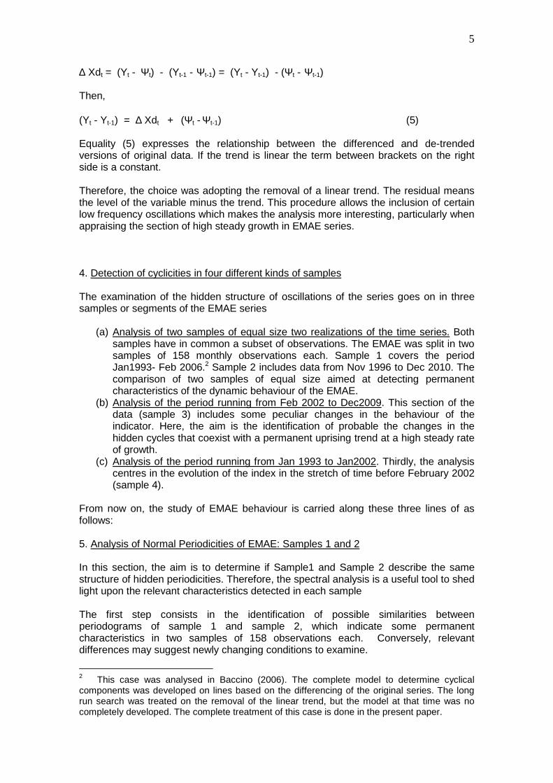
A1 -0.373681 1.323623 -2.343625 -4.640495 -1.740568 1.024531 A2 17.56638 -3.611871 -4.497417 0.5883313 1.598735 -1.915685 A 17.5704 3.8468 5.0714 4.6776 2.3634 2.1724 φ -1.5495 -1.2195 1.0904 -0.1261 -0.7429 -1.0797

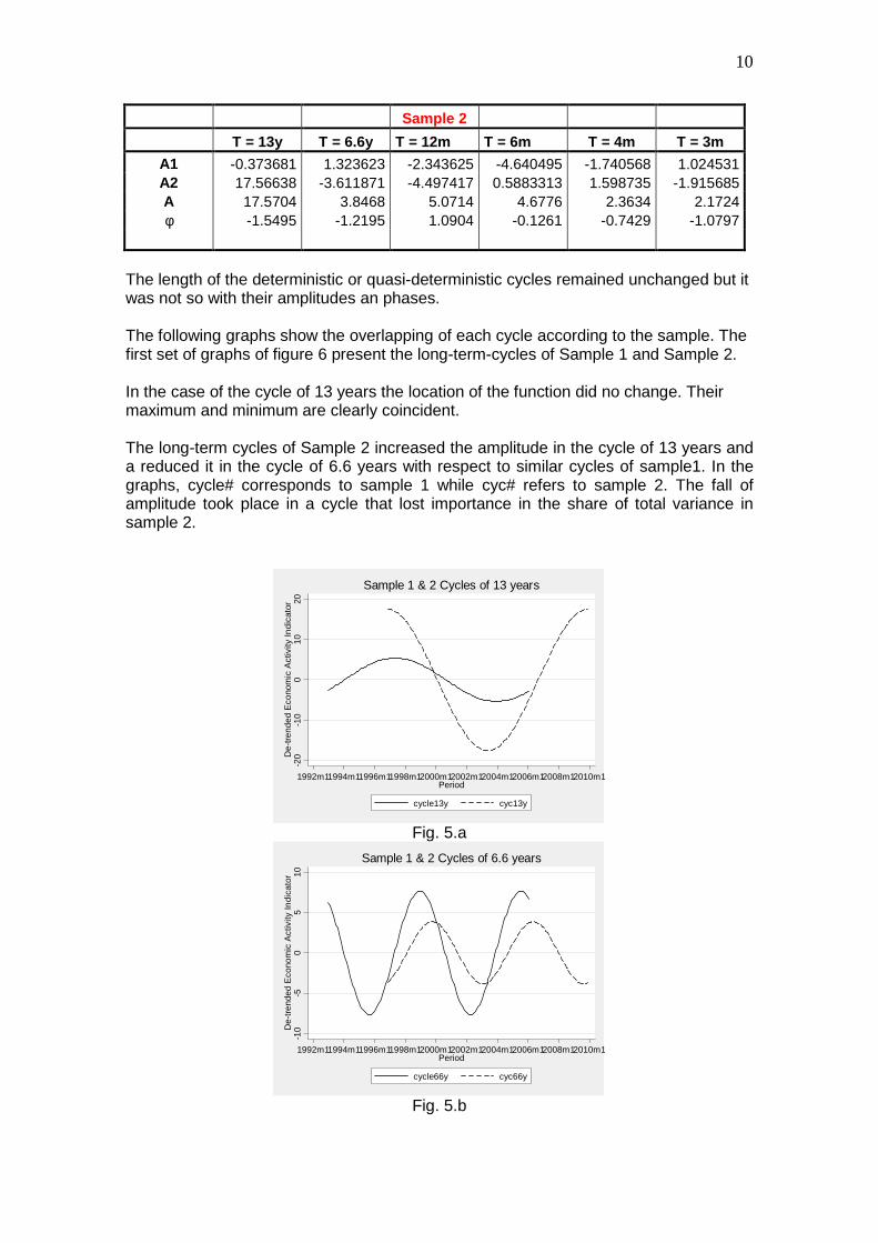
The length of the deterministic or quasi-deterministic cycles remained unchanged but it was not so with their amplitudes an phases. The following graphs show the overlapping of each cycle according to the sample. The first set of graphs of figure 6 present the long-term-cycles of Sample 1 and Sample 2. In the case of the cycle of 13 years the location of the function did no change. Their maximum and minimum are clearly coincident. The long-term cycles of Sample 2 increased the amplitude in the cycle of 13 years and a reduced it in the cycle of 6.6 years with respect to similar cycles of sample1. In the graphs, cycle# corresponds to sample 1 while cyc# refers to sample 2. The fall of amplitude took place in a cycle that lost importance in the share of total variance in sample 2.

-20

-10

010

20D

e-tr

ende

d E

cono

mic

Act

ivity

Indi

cato

r

1992m11994m11996m11998m12000m12002m12004m12006m12008m12010m1Period

cycle13y cyc13y

Sample 1 & 2 Cycles of 13 years

Fig. 5.a

-10

-50

510

De-

tren

ded

Eco

nom

ic A

ctiv

ity In

dica

tor

1992m11994m11996m11998m12000m12002m12004m12006m12008m12010m1Period

cycle66y cyc66y

Sample 1 & 2 Cycles of 6.6 years

Fig. 5.b

11

-10

-50

510

De-

tren

ded

Cyc

les

2005m1 2005m4 2005m7 2005m10 2006m1Period

arma1 arma2

Sample 1 and Sample 2 (arma1 & arma2)Stochastic cycles Models

Fig. 5.c

Fig. 5.c. shows the fittings of the stochastic cycles in sample 1 and sample 2. They adjust similar processes though there is a gap between both estimates. The arma1 model includes the cycle with a wavelength of 3 months while arma2 does not. This explains the gap. However, the periodicity of the stochastic component looks alike for the two series. The following graphs, (figure 6) present the seasonal cycles, with wavelengths of 12 months and less. Those cycles have bigger amplitudes in sample 2.

-50

5D

e-tr

ende

d E

cono

mic

Act

ivity

Indi

cato

r

2005m1 2005m4 2005m7 2005m10 2006m1Period

cycle12m cyc12m

Sample 1 & 2 Cycles of 12 months

Fig. 6.a

-50

5D

e-tr

ende

d E

cono

mic

Act

ivity

Indi

cato

r

2005m1 2005m4 2005m7 2005m10 2006m1Period

cycle6m cyc6m

Sample 1 & 2 Cycles of 6 months

Fig. 6.b

12

-2-1

01

2D

e-tr

ende

d E

cono

mic

Act

ivity

Indi

cato

r

2005m1 2005m4 2005m7 2005m10 2006m1Period

cycle4m cyc4m

Sample 1 & 2 Cycles of 4 months

Fig. 6.c

On the contrary, in the cycle of 4 months the maxima and minima take place at the same time in both samples (Fig. 6). By the way, this shift to the left with coincidence in maxima and minima does not obey to the different frequency definition. Both samples have the same number of observations and the definition of frequency intervals is the same for both samples. The seasonal movements have bigger amplitudes and the cycles show certain advance in time. That is, the cycle shifted to the left. On the contrary, those cycles, which lost importance in sample 2, have smaller amplitudes and shift to the right. The analysis of periodicities leads to the conclusion that the length of relevant cycles is the same though their amplitudes and phases undergo some changes. These modifications do not seem to be so large as to reflect serious parametric modifications. As it was said above, a similar situation applies to the stochastic components of the time series as follows from the ARMA models. At first sight, the series maintain the hidden structure of cyclicities (Fig. 5.c). In other words, it is no clear that there is a break in the pattern of stochastic periodicities between sample 1 and sample 2. 6. Sample 3. The stage of fast steady growth: a prime suspect? Sample 3 includes 95 observations in the period February 2002-December 2009. This segment of the series seems suspicious. Looking at the original series, one can detect that while the oscillations keep forms attached to similar patterns of the past, the trend entered a period of an unprecedented continuous growth at a very high rate, for eight years! Actually, this kind of growth seems hardly compatible with the situation that the Argentine economy is undergoing since 2002. There is no room in this paper to analyse further economic data in order to identify the causes of inconsistencies implicit in the EMAE series. However, anyone interested in the subject see Baccino (2005) for a description of the existence of persistent disequilibrium in the economy of Argentina. Coming back to the present work, the original series were also de-trended by a linear relationship and then a raw periodogram was built from the series obtained. The periodogram looked much the same like the others. It presented peaks in the same frequencies. In other words, it detected the most relevant cycles having the

13

similar lengths. The wavelengths of sample 3 are close but they do not coincide precisely with the ones from sample 2. This is so due to the different ranges of frequencies caused by different sample sizes.3 The variances at low frequencies have reduced ordinates. In this sample long-term cycles faded away. At the present, they give the impression that those oscillations are more probabilistic than deterministic. Now the relevant peaks are concentrated in the set of seasonal periodicities. In this sample, the deterministic long-term cycle disappeared. Any oscillation of this kind may take place in a wide range of frequencies. Therefore, they are part of the group explained by an ARMA model. The only relevant long-term element in the original series of sample 3 is the quasi-linear trend and this corresponds to the frequency zero. The removal of the linear trend from the series took off long-term deterministic cycles from the spectral density function.

050

100

150

Den

sity

.084 .168 .253 .347 .5Frequency (cycles per unit of time)

Sample 3Periodogram EMAE de-trended

Fig. 7

The cycles in Sample 3, with periods of twelve months and less, maintain their approximate length in almost all samples. As it was said above, the wavelength differs from the cycles of sample 2 in fractions of months. The lengths of cycles still are denoted in rounded figures but the regressions use the precise information. This simplifies description and the conclusions still arise without loss of generality.

3 The variable frequency is discrete and its values depend on the number of observations of the corresponding simple. Regressions calculated on the basis of different lengths obtained from different periodograms must necessarily produce some differences when evaluated at a given point of time.

14

Table III. Sample 3, Amplitude and Phase

Cycle 12 m Cycle 6m Cycle 4 m

A1 1.49594 -1.457756 -0.4181095 A2 -4.659816 -5.308368 -3.051077 A 4.8940 5.5049 3.0796 φφφφ -1.2602 1.3028 1.4346

-50

5D

e-tr

ende

d E

cono

mic

Act

ivity

Indi

cato

r

2002m1 2002m7 2003m1 2003m7Period

cyc6m cycle6cyc12m cycle12

A comparisonCycles in Sample 2 and Sample3

Fig. 8

Table III presents the regression coefficients of the cycle fittings and the amplitude and phase of the sine wave for each cycle in the seasonal oscillations of sample 3. Sample 3 produced a sine wave for a 12 month-cycle with smaller amplitude than in sample 2. This implies a shorter distance between maximum and minimum. On the other hand, the phase (φ) declines in the cycle of 12 months and increases in the 6-month and 4-month cycles. In the first two cycles, the sine wave shifts to the right, while in the other two cases the sine wave moves back to the left. The comparison between these seasonal periodicities and those detected in sample 2 are shown in figure 8. The opposite takes place in the cycles of length 6 and 4. Cycle 4 was not included in the graph. 7. Sample 4: The past evolution of economic activity as measured by EMAE The periodogram of sample 4 lost the cycle of 13 years and shows the highest peak for a cycle of 9 years. This case is accompanied by a group of minor oscillations distributed along a range of frequencies equal or smaller than the one corresponding to 1 year (or twelve months) length. The variances distributed along a band of lower frequencies reflect nondeterministic components except the peak at frequency 0.0091743, which is indicative of a cycle of 9 years peak-to-peak period.

15

050

100

150

Den

sity

.009 .083 .165 .248 .33 .413 .5Frequency (cycles per unit of time)

Sample 4Periodogram of EMAE de-trended

Fig. 9

This case expresses the old order. However, this sample has fewer observations than sample 1, so there appear some differences in the frequency range. The wavelengths of 12 months and less are different but very close to those of sample 1.

Table IV. Sample 4. Amplitude and Phase

Cycle 9y Cycle 12 m Cycle 6 m Cycle 4 m

A1 -2.370578 2.233972 -0.050966 0.4146675 A2 -5.610468 -3.694142 -3.990686 -2.587264 A 6.0907 4.3171 3.9910 2.6203 φφφφ 1.1710 -1.0269 1.5580 -1.4119

For sample 4, amplitudes slightly shrank in cycles of 12 and 6 months duration. Conversely, the amplitude increased in the four-month-cycle. The phase moved down in 12-month and up in 6-month, and down again in 4-month length. These displacements were very small. Remember that the difference between sampling size was smaller than in the comparisons of sample 3.

16

-4-2

02

4D

e-tr

ende

d E

cono

mic

Act

ivity

Indi

cato

r1998m4 1998m7 1998m10 1999m1 1999m4 1999m7

Period

cycle12m pastcy12mcycle6m pastcy6m

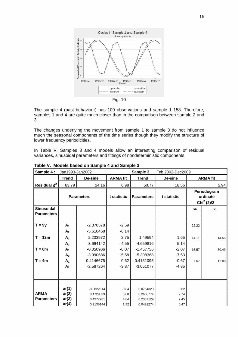
A comparisonCycles in Sample 1 and Sample 4

Fig. 10

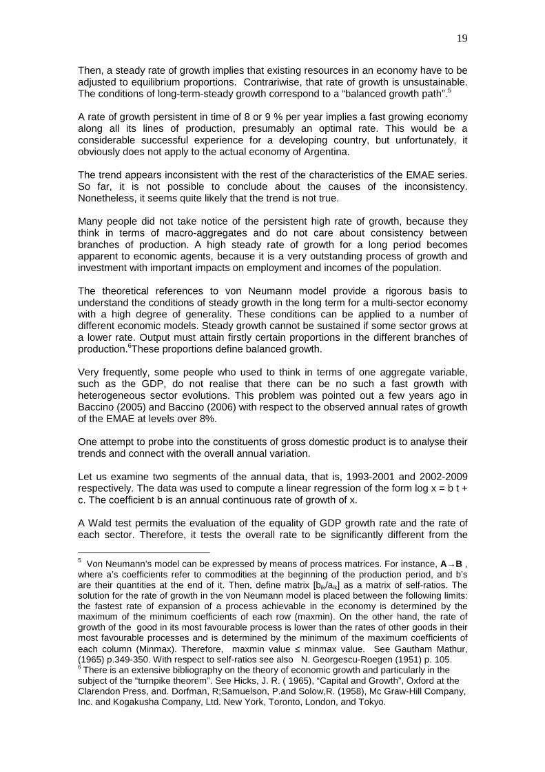
The sample 4 (past behaviour) has 109 observations and sample 1 158. Therefore, samples 1 and 4 are quite much closer than in the comparison between sample 2 and 3. The changes underlying the movement from sample 1 to sample 3 do not influence much the seasonal components of the time series though they modify the structure of lower frequency periodicities. In Table V, Samples 3 and 4 models allow an interesting comparison of residual variances, sinusoidal parameters and fittings of nondeterministic components. Table V. Models based on Sample 4 and Sample 3 Sample 4 : Jan1993-Jan2002 Sample 3 Feb 2002-Dec2009

Trend De-sine ARMA fit Trend De-sine ARMA fit

Residual σσσσ2222 63.79 24.16 6.98 50.77 18.56 5.94

Periodogram Parameters t statistic Parameters t statistic ordinate

Chi2 (2)/2

Sinusoidal S4 S3

Parameters

T = 9y A1 -2.370578 -2.59 22.22

A2 -5.610468 -6.14

T = 12m A1 2.233972 2.75 1.49594 1.65 14.11 14.55

A2 -3.694142 -4.55 -4.659816 -5.14

T = 6m A1 -0.050966 -0.07 -1.457756 -2.07 15.57 30.49

A2 -3.990686 -5.58 -5.308368 -7.53

T = 4m A1 0.4146675 0.62 -0.4181095 -0.67 7.67 12.00

A2 -2.587264 -3.87 -3.051077 -4.85

ar(1) -0.0822514 -0.84 0.0754323 0.62

ARMA ar(2) 0.4729039 6.08 0.2660774 2.74

Parameters ar(3) 0.4977281 4.84 0.2337129 2.45

ar(4) 0.2135144 1.92 0.0491274 0.47

17

ar(5) 0.0047423 0.04 0.1161346 1.18

ar(6) -0.0615316 -0.53 -0.0434773 -0.38

ar(7) -0.0957426 -0.71 -0.0488439 -0.46

ar(8) -0.0460003 -0.38 -0.0813948 -0.89

ar(9) -0.1611063 -1.38 -0.0472904 -0.4

ar(10) -0.282514 -2.57 -0.2457202 -2.23

ar(11) -0.2446629 -2.38 -0.2166053 -2.5

ar(12) 0.586896 5.74 0.6837688 6.41

ma(1) 0.790342 11.95 0.6827048 4.46

Portmanteau (Q) statistic = 26.7735 Portmanteau (Q) statistic = 28.2417 Prob > chi2(40) = 0.9459 Prob > chi2(40) = 0.9185 At the bottom of the table, Portmanteau (Q) statistics do not reject the null hypothesis of white noise in the residuals of each model. These are the signs of the completion of each model. The analysis of periodicities shows that the hidden structure is quite invariable, at least with respect to cycles of twelve months and less. 8. The analysis of Trend The trend is the most important distinctive component of the EMAE because it underwent some amazing change with respect to the past. The evolution under analysis corresponds to the period Feb 2002 – Dec 2009. The linear equation is Yt = 94.427 + 0.83440 trend + εt

(63.731) (31.132) R^2 = 0.912448 F(1,93) = 969.22 [0.0000] \sigma = 7.16366 DW = 0.995 RSS = 4772.573057 for 2 variables and 95 observations A recursive method was allows to examine the regression coefficients corresponding to different sizes of samples. The following figures present the constant and beta coefficients. The following graphs present the recursive computation of the intercept and slope of the linear trend within a band.

18

2003 2004 2005 2006 2007 2008 2009 2010

90

95

100

105Constant

2003 2004 2005 2006 2007 2008 2009 2010

-.5

0

.5

1

1.5Trend

Fig. 11 The band is defined by ± 2σ.around each coefficient. The trend coefficient is the trend slope, and it follows that the values obtained by the recursive method are vey close. Besides, the coefficient is very stable independently of the size of the sample. Another regression line was computed with the log transformation of EMAE. The slope is 0.006341 and expresses the average continuous rate of growth per month of 0.634%, or 7.6 % per annum. A trend rate of this importance for seven or eight years is very infrequently in an economy like Argentina, particularly because this kind of performance requires balanced growth. However, the difficulty in accepting such a high steady growth rate for a long period, follows from logical reasoning and this goes on with the help of economic theory. A high rate of growth sustained for a long period, requires that a particular proportions between productions should be attained and all branches of production of the economy grow, at least, at that rate. Otherwise, any sector growing at a lower rate becomes a bottleneck to growth. This follows from a general growth model such as von Neumann’s.4 This model was chosen because it admits complexities such as joint production and provides a useful analytical tool for viewing conditions for a steady growth.

4 Gautham Mathur, (1965). “The term ‘bottleneck goods’ is usually used with some imprecision and sometimes different senses of the term are confused with one another. Sometime one says, for instance in connection with the Neumann model, that the bottleneck good is that whose rate of growth is the least, i.e. the slowest-growing commodity; The first usage refers to the technological possibilities and the second to the amount of resources in a country at a particular moment. The two are of quite different natures. We shall distinguish between goods, which are bottlenecks to the rate of growth, and those, which are bottlenecks to the size of the national income in an economy.”

19

Then, a steady rate of growth implies that existing resources in an economy have to be adjusted to equilibrium proportions. Contrariwise, that rate of growth is unsustainable. The conditions of long-term-steady growth correspond to a “balanced growth path”.5 A rate of growth persistent in time of 8 or 9 % per year implies a fast growing economy along all its lines of production, presumably an optimal rate. This would be a considerable successful experience for a developing country, but unfortunately, it obviously does not apply to the actual economy of Argentina. The trend appears inconsistent with the rest of the characteristics of the EMAE series. So far, it is not possible to conclude about the causes of the inconsistency. Nonetheless, it seems quite likely that the trend is not true. Many people did not take notice of the persistent high rate of growth, because they think in terms of macro-aggregates and do not care about consistency between branches of production. A high steady rate of growth for a long period becomes apparent to economic agents, because it is a very outstanding process of growth and investment with important impacts on employment and incomes of the population. The theoretical references to von Neumann model provide a rigorous basis to understand the conditions of steady growth in the long term for a multi-sector economy with a high degree of generality. These conditions can be applied to a number of different economic models. Steady growth cannot be sustained if some sector grows at a lower rate. Output must attain firstly certain proportions in the different branches of production.6These proportions define balanced growth. Very frequently, some people who used to think in terms of one aggregate variable, such as the GDP, do not realise that there can be no such a fast growth with heterogeneous sector evolutions. This problem was pointed out a few years ago in Baccino (2005) and Baccino (2006) with respect to the observed annual rates of growth of the EMAE at levels over 8%. One attempt to probe into the constituents of gross domestic product is to analyse their trends and connect with the overall annual variation. Let us examine two segments of the annual data, that is, 1993-2001 and 2002-2009 respectively. The data was used to compute a linear regression of the form log x = b t + c. The coefficient b is an annual continuous rate of growth of x. A Wald test permits the evaluation of the equality of GDP growth rate and the rate of each sector. Therefore, it tests the overall rate to be significantly different from the

5 Von Neumann’s model can be expressed by means of process matrices. For instance, A→B , where a’s coefficients refer to commodities at the beginning of the production period, and b’s are their quantities at the end of it. Then, define matrix [bik/aik] as a matrix of self-ratios. The solution for the rate of growth in the von Neumann model is placed between the following limits: the fastest rate of expansion of a process achievable in the economy is determined by the maximum of the minimum coefficients of each row (maxmin). On the other hand, the rate of growth of the good in its most favourable process is lower than the rates of other goods in their most favourable processes and is determined by the minimum of the maximum coefficients of each column (Minmax). Therefore, maxmin value ≤ minmax value. See Gautham Mathur, (1965) p.349-350. With respect to self-ratios see also N. Georgescu-Roegen (1951) p. 105. 6 There is an extensive bibliography on the theory of economic growth and particularly in the subject of the “turnpike theorem”. See Hicks, J. R. ( 1965), “Capital and Growth”, Oxford at the Clarendon Press, and. Dorfman, R;Samuelson, P.and Solow,R. (1958), Mc Graw-Hill Company, Inc. and Kogakusha Company, Ltd. New York, Toronto, London, and Tokyo.

20

sector rate. This procedure holds for a group of sectors producing goods and for another group producing services. Segment 1993-2001 The growth-rate of GDP trend is 1.87% per year.7 Agriculture and livestock, Fishery, Mining and Construction are growing faster that GDP but their differences are not significant. On the other hand, Manufactures and Electricity, Gas and Water grow slower than GDP though their differences are significant.

Table VI. Segment 1993-2001 Sector rates of growth (continuous) and significance level of the difference with the GDP rate g = 0.018681

Sector growth rates F( ) Probability

Agr. Livestock 0.0266128 1.62 0.2439 Fisheries 0.0211055 0.151 0.7089 Mining 0.0332171 5.44 0.0525 Manufacturing -0.000751 9.71 0.0169 ElectGasWa 0.0600108 43.94 0.0003 Construction 0.008308 2.79 0.1403 Goods 0.0117978 1.22 0.3061 Trade 0.006094 4.08 0.0833 Hotels &rest. 0.0350567 6.9 0.0341 Transport 0.0473201 21.1 0.0025 Finance 0.0774742 89.92 0.0000 Real estate 0.0197588 0.029875 0.8677 Pub. Adm. -0.001287 10.26 0.015 Edu.&Health 0.0278921 2.18 0.1831 Pers.services 0.0268825 1.73 0.2298 Services 0.0253208 1.13 0.3222

Among sectors producing services, Trade, Real Estate, Education & Health and Personal services, grow faster than the overall GDP rate, but the differences are not significant. Those having significant differences are Hotels and restaurants, Transport and Financial with bigger rates than GDP and Public Administration with smaller growth than the overall rate. Segment 2002-2009 Here the picture is quite different from above. The GDP trend growth-rate is 7.54% per year. Manufactures grows faster than GDP though the difference is not significant. The sectors producing goods that have significant differences are Construction (growing

7 Remember that this annual rate is continuous. A transformation such as ( erate -1) gives the equivalent discrete annual rate.

21

faster) and Agriculture and livestock, Fishery, Mining and Electricity, gas & water, whose rates of growth are below the mean. Production of Services also shows differences with respect to the other segment. Hotels & restaurants and Personal services grow less than GDP but the difference is not significant. Trade, Transport and Finance have significant and higher rhythms of growth while Real estate, Public Administration and Education & Health grow slower than GDP. Now, the differences of trend behaviour become clear. Segment 1993-2001 looked as expected. Conversely, Segment 2002-2009 showed a peculiar behaviour. Firstly, there is a very high rate of growth for a long time.

Table VII. Segment 2002-2009 Sector rates of growth (continuous) and significance level of the difference with the GDP rate g = 0.0754371

Sector growth rates F( ) Probability

Agr. Livestock 0.026787 135.23 0.0000 Fisheries 0.0204045 168.11 0.0000 Mining 0.0074715 256.42 0.0000 Manufacturing 0.076588 0.07352 0.7954 ElectGasWa 0.048144 41.35 0.0007 Construction 0.14468 266.15 0.0000 Goods 0.0724495 0.495 0.5079 Trade 0.0893042 10.67 0.0171 Hotels &rest. 0.0668512 4.09 0.0895 Transport 0.1178165 99.7 0.0001 Finance 0.0984681 29.44 0.0016 Real estate 0.0451058 51.07 0.0004 Pub. Adm. 0.0336629 96.87 0.0001 Edu.&Health 0.0400348 69.57 0.0002 Pers.services 0.069836 1.74 0.2351 Services 0.0708272 1.18 0.3191

The sectors whose rates of growth are not significantly different from the overall rate are Hotels & restaurants and Personal services. The only goods producers that are closer in growth is Manufacturing. The rest of goods producers keep a slower pace behind, except Construction, which has a significant bigger growth rate. In the area of services producers, fast growth being significantly different from the overall rate corresponds to Trade, Transport and Finance. Contrariwise, real estate, public administration and education & Health grew much less than the GDP. Summing up, greatest expansion took place in services activities and only in manufacturing and constructive activities. The rest of goods producers had smaller rates than the average. Obviously, this situation cannot be described as “balanced growth”.

22

The annual rates of expansion of some GDP components are shown in the Annex 2. Even more, this picture seems rather inconsistent unless one accepts that there might be problems of valuation of aggregates in real terms. In a period where the prices are distorted, and there are many problems of detection between prices and quantities from monetary values, the identification of modifications in the levels of economic activities are very hard. The importance of these drawbacks might be associated with the levels of the growth rates. The sign that some problem exists is the permanent high rate of economic activity in the long run. That high level for the average rate produces a false impression of balanced growth in the long term. The identification of causes of the inconsistent data should emerge from an audit of the process of construction of national accounts. So far, only inconsistencies come up because of economic and statistical interpretations. The macroeconomic variables do not reflect variations in real variables in a correct way. The analysis of Sample 3 showed only relevant cyclicities in periods of 12 months and less. Relevant long-term cycles were absent in the spectral density estimate, while they were present in the previous segment. Those variations are absorbed in the annual figures for macro-aggregates. 9. An exercise of simulation with EMAE time series Now, a simulation exercise will be useful to establish some alternative evolution of economic activity and later to examine the effects of substituting the trend by another with different rhythm of accumulation. The simulation exercise starts by manipulating the original series and creating a band of variation for the EMAE since 2002 onwards. A couple of alternative evolutions will result from the simulation. Then, these results will help to interpret a possible way back to the original figures. The first part of the simulation consists in replacing the trend in the original series by the trend identified in the previous segment of the EMAE series. The deviations of the indicator from the original trend were added to the new trend and a new evolution was produced. This estimate is included in the variable ‘newseries’. This substitution altered the original series and gave an indicator which retains the hidden periodicities analysed before and produced a path that reduces the long term growth though it keeps moving up in a damped way. The outstanding feature of this simulated series is that the sharp fall in the indicator in 2002 was neglected. Moreover, it overstates the level of monthly economic activity. No doubt, ‘newseries’ does not capture a break in the trend, both in the slope and the intercept. The recursive regression made before shows a wider band of variation in the fist years, and this is very sensitive in the case of the constant. A new alternative path emerges by replacing the trend by another, at a level of ¾ of the previous one. The ‘new2series’ variable provided a lower bound for the analysis. The idea of obtaining a lower-bound-series, being proportional to the traditional trend, aims to limit any further assumptions about trend. Both newseries and new2series variables are shown in Annex 1.

23

In this analysis, only two separate trends are available: one corresponds to Sample 4 which is reliable, and another refers to sample 3 which is inconsistent. The removal of trend in sample 3 was replaced by an extension of trend of Sample 4. The assumption of a lower bound trend as a proportion of the old trend implies to reduce both slopes and intercept in the same degree. In fact, the objective is to establish limits for the real series. No further assumptions are needed.

8010

012

014

016

018

0E

MA

E

1992m11994m11996m11998m12000m12002m12004m12006m12008m12010m1Period

emae09 newseriesnew2series

Newseries and New2seriesSimulation of EMAE series

Fig. 12

The representation of the original and the new estimates is in figure 12. The true evolution should be somewhere in between the estimates. In fact, the true EMAE series should be between the newseries and new2series. Perhaps, it is not absolute linear particularly at the beginning, that is during the year 2002. The first months of recovery might have grown fast including the so-called bounce effect. The real series should reflect the influence of the low levels of 2002 and the high levels of 2003 onwards. By the way, it is interesting to compare original annual growth rates with those obtained from the simulations. The simulations present rates of growth much more consistent with the Argentine experience Now, let us turn the exercise upside down. Suppose that the economy moved along the true path and that the statistics were readjusted. For instance, that readjustment could have been the removal of the actual trend component and its substitution by the trend that implies high steady rate of growth.

24

The result would have been the series published by the INDEC. All the spectral studies performed before applies to the series. This could be a way to introduce the inconsistent trend into the figures, and this presumably started in the last part of 2002.

Table VIII. EMAE Annual rates of growth %

EMAE Simulations Year INDEC newseries new2series

2002 -10.9 6.6 -18.2 2003 8.8 2.4 -0.2 2004 9.0 1.4 1.3 2005 9.2 2.2 2.5 2006 8.5 2.2 2.5 2007 8.7 3.1 3.6 2008 6.8 1.6 1.7 2009 0.8 -5.0 -7.1

. Of course, many would say that the introduction of the inconsistent trend may be due to problems of data, defective means to adjust sampling data to the total economy, and particularly incomplete deflation in prices by wrong price indexes, and so on. Surely, it is likely that many of those factors might have altered the data used in constructing the EMAE indicator. Nonetheless, what is hard to believe is that all these problems did not affect the hidden structure of cycles, and created a neatly linear trend. Therefore, it seems more probable there was a deliberate removal of trend with the aim to extending forward the conditions of the beginning of the recovery in 2002. 10. Concluding Remarks From the comparison of raw periodograms of samples 1 and 2, emerges that the peak frequencies are quite similar in both spectral density functions. This is particularly so in those cases representing seasonal periodicities. Both samples are combinations of two different behaviours detected in sample 3 and sample 4 with dissimilar weights. On the other hand, with respect to samples 1 and 2, some differences prevail in lower frequencies. They denote cycles of long duration. The periodogram of sample 2 presents more important variances than the one in the other sample. These changes produce a tradeoff in the amplitude of the long-term-cycle. The amplitude of the cycle of 13 years increased while it decreased in the cycle of 6.6 years in sample 2 with respect to sample 1. Clearly, sample 2 has more weight in components of lower frequencies than the other does. These changes are seen because de-trending applied to the series kept some important lower frequencies and reduced those of seasonal kind. This applied both to deterministic and probabilistic cycles. A general conclusion about the comparison of the samples with equal numbers of observations is that their structures of periodicities remained quite similar. By the way, the lengths of the most relevant cycles did not change though there were modifications in amplitude of each sinusoidal wave.

25

Incidentally, someone could say that in general the periodic components both deterministic and stochastic did not undergo significant modification in the present study. The indicator EMAE seems to have a definite structure of oscillations. Nonetheless, the important changes of behaviour in long-term aspects took place from sample 4 to sample 3, in the components of the combination already mentioned. Furthermore, this comparison refers to the segment running from Jan 1993 to Jan 2002 against the period Feb 2002 - Dec 2009. This analysis identifies in more detail aspects not clearly exposed in the previous comparison. Both cases maintain similar characteristics in terms of seasonal patterns. They also have their stochastic periodicities modelled in similar ARMA forms. Notwithstanding, in sample 3 the nearly deterministic cycles of long length seem absent while those cyclicities of length equal or shorter than twelve months appear as the most relevant. Low frequency became less important and the main element in departing from the usual experience of EMAE is an increasing linear trend, which appears as a cycle of infinite length. The high steady rate around 8% per year coexists with the disappearance of long term cycles detected in previous years. On the other hand, the segment Jan 1993-Jan 2002 (sample 4) presents an important deterministic cycle of nine years of duration. The above analysis leads to the conclusion that the most striking difference between both segments of the series (samples 3 & 4) appears in both cycles and trend in the long term. As far as economic interpretation is concerned, some changes in the behaviour of the economy should produce modifications in the general dynamic framework. There is no economic reason whatsoever which justifies the long period of permanent high rates of growth in Argentina in the period under analysis. Such a kind of growth requires all sectors growing at least at that speed. In other words, the requirement is a permanent state of balanced expansion; otherwise, the steady growth is unsustainable. However, there is no further evidence of balance growth for Argentina if more information is added. Therefore, the observed trend in sample 3 is inconsistent. This trend is the only component of the time series that changed with respect to the traditional behaviour, while the seasonal cyclicity remained the same. Nevertheless, should the process of adjustment of the stocks of resources have altered the cyclicity? It seems plausible that the cyclicity should have been altered with cycles of lengths larger than 12 months. “Any time-series can of course be analysed, by well-known statistical methods, into trend and fluctuations about the trend. We have a Theory of Fluctuations to deal with the fluctuations; let us match it with a Theory of Growth, to deal with the trend. That, I am sure, is the way in which the matter has often been taken; but one of the troubles is that when it is taken in that way it does not come out quite right…We have no right to conclude, from the mere existence of the statistical device, that the economic forces making for trend and for fluctuation are any different, so that they have to be analysed in different ways.”8

8 J.R. Hicks (1965) p. 4.

26

This quote clearly warns about a similar problem to the one underlying the construction of the EMAE, which shows that those who make the indicator were not aware of its implications on growth theory. They should be the first to notice what meant the persistency of a very high growth rates for several years. The next question to come out is: If collected data led to the original series, what transformed the unknown real trend into an inconsistent one? So far, it is likely that some substitution of the trend arose, being intentionally or not, during the construction of the series. There are also chances that a defective process of collecting and deflating data may have influenced the construction of the series. The analysis of trend in several components of gross domestic product shows an important contribution of services to growth. However, even when the latter were true, there would still be a very small probability that the distortions spread through time to produce such a steady rate of growth of EMAE. The simulation performed at the end of the study described how the peculiar trend could be introduced into the series by replacing actual long-term movements without any alteration on the rest of the seasonal components. It was also possible that in the first part of the path, say along most of the year 2002, the evolution was real, and later, the recovery was artificially extended onwards, due to problems of deficient information. It seems that the macro-aggregates do not reflect adequately changes in quantities. If this is true, the quality of information should be warranted in the process of constructing the national accounts. Anyway, the result of this study is that the section that raised doubts presents inconsistency between components in the time series. Further study of the causes should be done by other methods, particularly on the process of data construction, since the identification of causes is outside the aim of the present analysis. References: * Baccino, Osvaldo E. (2006) “Comportamientos Cíclicos en la Actividad Económica de la Argentina 1993-2006”, XLI Reunión Anual de la Asociación Argentina de Economía Política (AAEP), Salta, 2006. http://www.aaep.org.ar. * Baccino, Osvaldo E. (2005), “A Case of a Persistent Disequilibrium Policy: Argentina since 2002”, XL Reunión Anual de la Asociación Argentina de Economía Política (AAEP), La Plata, Provincia de Buenos Aires, 2005. Internet http://www.aaep.org.ar. * Bloomfield, Peter, (2000), “Fourier analysis of time series: an introduction”, Wiley Series in Probability and Statistics, John Wiley & Sons, second Edition, U.S.A. * Dorfman, R;Samuelson, P.and Solow,R. (1958), Mc Graw-Hill Company, Inc. and Kogakusha Company, Ltd. New York, Toronto, London, and Tokyo. * Hicks, J. R., (1965), “Capital and Growth”, Oxford At The Clarendon Press. * Nicholas Georgescu-Roegen, (1951), “The Aggregate Linear Production Function and its Application to von Neumann’s Economic Model”, Activity Analysis of Production and Allocation. Proceedings of a Conference. Edited by Tjalling C. Koopmans. John Wiley & Sons. New York.

27

* Mathur, Gautham, (1965), “Planning for Steady Growth”, Basil Blackwell, Oxford. * Gottman, John M. (1981), “Time-series Analysis. A comprehensive introduction for social scientists”, Cambridge University Press. * Granger, W.J. and Newbold, Paul, (1986) “Forecasting Economic Time Series”, Second Edition, Academic Press, Inc.

* Instituto Nacional de Estadística y Censos (INDEC), (Octubre 2002), “Sistema de Cuentas Nacionales Argentinas. Año Base 1993. Estimador Mensual de Actividad Económica: Fuentes de información y métodos de estimación”. 15 metodologías * Instituto Nacional de Estadística y Censos (INDEC), EMAE y Cuentas Nacionales por Internet. Annex 1: Original Data from the National Institute of Statistics (INDEC) and Simulations obtained in the study (old trend & lower bound)

Monthly Economic Activity Indicator (EMAE) 1993 = 100 (*) Simulations

Period EMAE Period EMAE Newseries New2series 1993m1 88.2 2001m7 114.9 1993m2 85.5 2001m8 112.3 1993m3 100.8 2001m9 106.6 1993m4 101.6 2001m10 106.3 1993m5 103.5 2001m11 107.2 1993m6 101.7 2001m12 102.2 1993m7 102.4 2002m1 87.0 1993m8 102.0 2002m2 89.1 113.8 83.8

1993m9 103.3 2002m3 98.9 122.9 92.9

1993m10 101.2 2002m4 103.0 126.3 96.3

1993m11 105.3 2002m5 106.9 129.6 99.5

1993m12 104.4 2002m6 102.6 124.6 94.4

1994m1 95.2 2002m7 102.9 124.2 94.0

1994m2 92.1 2002m8 99.7 120.3 90.1

1994m3 108.2 2002m9 98.5 118.5 88.2

1994m4 108.4 2002m10 99.5 118.8 88.5

1994m5 110.8 2002m11 102.1 120.7 90.4

1994m6 107.4 2002m12 103.3 121.2 90.9

1994m7 106.2 2003m1 91.3 108.6 78.1

1994m8 107.5 2003m2 93.8 110.4 79.9

1994m9 107.8 2003m3 104.9 120.8 90.3

1994m10 106.2 2003m4 110.3 125.5 95.0

1994m11 110.7 2003m5 114.5 129.1 98.5

1994m12 109.5 2003m6 111.8 125.7 95.1

1995m1 94.9 2003m7 112.8 126.0 95.4

1995m2 97.0 2003m8 108.5 121.0 90.3

1995m3 109.9 2003m9 110.5 122.4 91.6

1995m4 102.0 2003m10 112.1 123.3 92.5

1995m5 108.0 2003m11 113.0 123.5 92.7

1995m6 104.7 2003m12 115.6 125.4 94.6

1995m7 103.7 2004m1 100.6 109.8 78.9

28

1995m8 102.5 2004m2 103.3 111.8 80.9

1995m9 101.0 2004m3 118.7 126.5 95.5

1995m10 102.5 2004m4 117.5 124.6 93.6

1995m11 105.2 2004m5 121.6 128.1 97.0

1995m12 102.3 2004m6 121.6 127.4 96.3

1996m1 93.9 2004m7 120.9 126.0 94.9

1996m2 97.7 2004m8 119.4 123.9 92.7

1996m3 108.5 2004m9 120.4 124.2 92.9

1996m4 109.4 2004m10 120.2 123.3 92.0

1996m5 113.2 2004m11 125.3 127.7 96.4

1996m6 108.1 2004m12 126.7 128.5 97.1

1996m7 113.4 2005m1 108.8 109.9 78.5

1996m8 111.3 2005m2 111.7 112.1 80.7

1996m9 107.9 2005m3 127.9 127.6 96.2

1996m10 112.9 2005m4 131.1 130.2 98.6

1996m11 113.3 2005m5 135.5 133.9 102.3

1996m12 112.5 2005m6 131.6 129.3 97.7

1997m1 104.8 2005m7 130.2 127.2 95.6

1997m2 105.4 2005m8 132.2 128.6 96.9

1997m3 115.0 2005m9 131.6 127.3 95.6

1997m4 121.0 2005m10 131.5 126.5 94.8

1997m5 120.1 2005m11 137.1 131.4 99.6

1997m6 116.3 2005m12 137.2 130.9 99.0

1997m7 121.0 2006m1 118.3 111.3 79.4

1997m8 118.0 2006m2 121.8 114.1 82.2

1997m9 121.4 2006m3 138.8 130.4 98.5

1997m10 122.3 2006m4 139.1 130.1 98.1

1997m11 121.0 2006m5 147.0 137.3 105.3

1997m12 121.4 2006m6 142.9 132.5 100.4

1998m1 108.3 2006m7 142.3 131.2 99.1

1998m2 110.1 2006m8 143.3 131.6 99.4

1998m3 126.2 2006m9 142.8 130.4 98.2

1998m4 126.8 2006m10 144.4 131.3 99.1

1998m5 127.6 2006m11 149.2 135.4 103.2

1998m6 127.7 2006m12 147.3 132.9 100.6

1998m7 126.6 2007m1 128.4 113.3 80.9

1998m8 122.5 2007m2 131.3 115.5 83.1

1998m9 123.0 2007m3 149.4 132.9 100.5

1998m10 121.2 2007m4 150.4 133.3 100.8

1998m11 121.8 2007m5 160.5 142.7 110.2

1998m12 120.2 2007m6 155.3 136.8 104.3

1999m1 104.8 2007m7 155.1 135.9 103.4

1999m2 108.0 2007m8 157.2 137.4 104.7

1999m3 123.4 2007m9 153.9 133.4 100.7

1999m4 121.0 2007m10 159.3 138.1 105.4

1999m5 121.7 2007m11 162.2 140.3 107.6

1999m6 120.6 2007m12 159.5 137.0 104.2

1999m7 117.7 2008m1 142.2 119.0 86.2

1999m8 117.7 2008m2 144.2 120.3 87.5

1999m9 117.9 2008m3 157.5 132.9 100.0

1999m10 116.0 2008m4 165.3 140.1 107.1

1999m11 120.6 2008m5 172.3 146.4 113.4

1999m12 123.1 2008m6 165.0 138.4 105.4

2000m1 103.8 2008m7 167.6 140.3 107.3

29

2000m2 109.0 2008m8 165.9 138.0 104.9

2000m3 122.8 2008m9 165.1 136.5 103.4

2000m4 119.1 2008m10 166.6 137.3 104.1

2000m5 122.8 2008m11 168.4 138.4 105.2

2000m6 120.0 2008m12 165.5 134.9 101.6

2000m7 118.1 2009m1 144.4 113.1 79.8

2000m8 117.6 2009m2 147.3 115.3 82.0

2000m9 115.4 2009m3 161.3 128.7 95.3

2000m10 115.0 2009m4 166.1 132.8 99.4

2000m11 117.3 2009m5 170.2 136.2 102.7

2000m12 120.4 2009m6 162.5 127.8 94.3

2001m1 104.3 2009m7 165.0 129.7 96.1

2001m2 105.8 2009m8 165.9 129.9 96.3

2001m3 118.8 2009m9 165.8 129.1 95.5

2001m4 119.1 2009m10 167.6 130.2 96.6

2001m5 123.3 2009m11 172.1 134.1 100.4

2001m6 118.8 2009m12 173.7 135.0 101.2

(*) Source: INDEC Annex 2: Annual rates of growth of GDP of Argentina (*)

Sector 2002 2003 2004 2005

Agriculture, livestock, and forestry -1.7 7.0 -1.0 11.7

Fishery -19.3 1.2 -19.1 -14.3

Stone and clay mining and quarrying -3.7 3.7 -0.4 -0.2 Manufacturing Industry -11.0 16.0 12.0 7.5 Electricity, Gas and water -3.0 6.9 6.5 5.0 Construction -33.4 34.4 29.4 20.4 SECTORS PRODUCING GOODS -11.7 14.5 10.5 9.5 Wholesale and Retail Trade and Repair -18.5 12.9 13.6 9.8 Hotels and restaurants -8.3 6.0 7.0 7.9 Transportation, Warehousing and Communications -7.9 8.2 13.4 14.8 Finance and Insurance -19.7 -15.8 -5.5 17.5 Real estate, Business and rental activities -5.6 3.9 4.3 4.5 Public Administration and Defense -0.9 1.1 1.8 3.3 Medical, educational, non profit organisations -0.3 2.7 2.9 4.2 personales and domestic help -9.8 4.7 9.1 9.8

SECTORS PRODUCING SERVICES -9.2 4.2 6.8 8.4

Sector 2006 2007 2008 2009

Agriculture, livestock, and forestry 1.5 10.3 -2.7 -15.8

Fishery 63.5 -6.4 4.1 -11.9

Stone and clay mining and quarrying 3.0 -0.5 1.1 -1.1

30

Manufacturing Industry 8.9 7.6 4.5 -0.5 Electricity, Gas and water 5.0 5.7 3.4 0.9 Construction 17.9 9.9 3.7 -3.8 GOODS PRODUCING SECTORS 8.8 7.9 2.9 -3.5 Wholesale and Retail Trade and Repair 8.0 11.1 7.9 -0.2 Hotels and restaurants 7.3 8.2 7.7 0.7 Transportation, Warehousing and Communications 13.5 13.7 12.1 6.5 Finance and Insurance 22.1 18.6 17.4 0.8 Real estate, Business and rental activities 4.2 4.7 6.3 4.0 Public Administration and Defense 4.5 3.7 3.9 5.1 Medical, educational, non profit organisations 4.3 4.8 4.5 4.3 personales and domestic help 7.7 6.4 6.2 3.8 SERVICES PRODUCING SECTORES 8.1 8.7 8.2 3.2

(*) The rates were computed on data from National Accounts of Argentina.