Embed Size (px)
Citation preview

Universidade do MinhoEscola de Psicologia
Maio de 2013
Ana Catarina Gonçalves Vieira de Castro
Experiments on temporal learning: from intraand interdimensional gradients to ageneralization-based account of complexbehavior
Ana
Cat
arin
a G
onça
lves
Vie
ira d
e C
astr
oE
xpe
rim
en
ts o
n t
em
po
ral l
ea
rnin
g:
fro
m in
tra
an
d in
terd
ime
nsi
on
al
gra
die
nts
to
a g
en
era
liza
tio
n-b
ase
d a
cco
un
t o
f co
mp
lex
be
ha
vio
rU
Min
ho|2
013


Tese de Doutoramento em PsicologiaEspecialidade de Psicologia Experimental e Ciências Cognitivas
Trabalho realizado sob a orientação do Professor Doutor Armando Domingos Batista Machado
Universidade do MinhoEscola de Psicologia
Maio de 2013
Ana Catarina Gonçalves Vieira de Castro
Experiments on temporal learning: from intraand interdimensional gradients to ageneralization-based account of complexbehavior


iii
Acknowledgements
Quero agradecer a todos aqueles que contribuíram para que este projecto fosse
possível.
Em primeiro lugar, ao Professor Armando Machado, por ter abraçado este
projecto comigo. Pelo modelo que foi para fim durante estes anos, pelo espírito crítico,
pela forma entusiasta com que partilha o seu conhecimento e pela sua incessante busca
de uma ciência melhor. Aquilo que sou hoje enquanto investigadora devo-o a si em
grande parte.
Ao François e ao Jeremie pelo feedback sobre o meu trabalho e pelo
conhecimento transmitido durante as suas estadias na Universidade do Minho. Ao
Randy e ao Marco. A todos os colegas que me foram acompanhando no Laboratório de
Aprendizagem e Comportamento Animal da Universidade do Minho, pelo
companheirismo, ajuda e troca de ideias. Em especial ao Luís e ao Tiago, pela amizade
que ficou.
Ao Professor Gerson Tomanari por me ter recebido na Universidade de São
Paulo e me ter possibilitado uma experiência tão rica a nível académico e pessoal. Aos
restantes professores da Universidade de São Paulo que tive o prazer de conhecer, em
especial à Miriam, por toda a ajuda e simpatia. Aos colegas de São Paulo e em especial
ao Saulo, Peter, Cândido, Hernando e Rafa pela amizade e pelas infindáveis horas de
discussão.
À Tathi e novamente ao Saulo, por me terem acolhido tão bem e por todo o
apoio e carinho.
A toda a minha família. Ao mano, aos avós, tios, tias, primos e primas. Mas em
especial aos meus pais, por todo o amor, paciência e compreensão.
Aos meus amigos. À Tuxinha, à Olga, à Sara, à Cláudia, à Marina, à Susana e ao
Rogério. À Piri e à Portela. Ao Rui, ao Vítor, ao Artur e ao João.
À Aimy, pela companhia.

iv

v
Title
Experiments on temporal learning: from intra and interdimensional gradients to a
generalization-based account of complex behavior
Abstract
In a temporal double bisection task pigeons learn two temporal discriminations.
They learn to choose Red over Green after 1-s samples and Green over Red after 4-s
samples (Type 1 discrimination) and to choose Blue over Yellow after 4-s samples and
Yellow over Blue after 16-s samples (Type 2 discrimination). Subsequently, pigeons
choose between Green and Blue after samples ranging from 1 to 16 s and, even though
the two choices were previously associated with the same duration of 4 s, the
probability of choosing Green increases with sample duration – the context effect. This
complex result seems to suggest relational learning because Green was associated with
the longer sample in the Type 1 discrimination and Blue was associated with the shorter
sample in the Type 2 discrimination.
The first goal of this thesis was to investigate whether the context effect could be
explained from the combination of the temporal generalization gradients for Green and
Blue induced by the discriminative training in a double bisection task, following a
strategy used in other stimulus dimensions. The timing model Learning-to-Time (LeT)
instantiates this generalization-based account of the context effect. The second goal of
this thesis was to investigate whether both the temporal generalization gradients and the
context effect were consistent with LeT.
In contrast to more familiar stimulus dimensions, such as light wavelength or
tone frequency, little research has been directed to the study of generalization gradients
in the temporal domain. Little is known about their features and the variables that affect
them. The third goal of this thesis was to explore the effects of different training
protocols, namely the intradimensional and interdimensional protocols, on the temporal
generalization gradient.
The thesis comprises three studies. Study 1 and Study 2 addressed the first two
goals and also investigated the shape of intradimensional temporal generalization
gradients. Study 3 explored the effects of interdimensional training on the temporal
generalization gradient.

vi
In Study 1, pigeons learned a simplified version of the double bisection task,
whereby only the two responses critical to the context effect, Green and Blue, were
trained. Namely, pigeons learned to peck Green after 4 s but not to peck it after 1 s and
to peck Blue after 4 s but not to peck it after 16 s. Next, temporal generalization
gradients for Green and Blue were obtained by varying the sample duration from 1 to
16 s. Finally, pigeons were given a choice between Green and Blue after samples
ranging from 1 to 16 s.
Study 2 extended Study 1 to a standard double bisection task and, additionally, it
involved testing with durations outside the training range. First, pigeons learned to
choose Red over Green after 2 s and Green over Red after 6 s and to choose Blue over
Yellow after 6 s and Yellow over Blue after 18 s. Second, sample duration was varied
from 0.7 to 51.4 s and temporal generalization gradients for Green (over Red) and for
Blue (over Yellow) were obtained. And third, pigeons were given a choice between
Green and Blue after samples ranging from 0.7 to 51.4 s.
The results of the two studies showed that a) the generalization gradients for
Green and Blue were either ramp-like or bitonic; b) the preference for Green over Blue
increased with sample duration – the context effect; c) the two generalization gradients
predicted the observed context effect well; and d) the LeT model accounted for the
major trends in the data.
In Study 3 pigeons were trained to discriminate the presence and the absence of
a t-s sample: they learned to choose Green after the illumination of a houselight for t s
and to choose Red after a period in the darkness. Subsequently, the houselight duration
was varied and the preference for Green was assessed to obtain temporal generalization
gradients. The results showed negative-exponential-like temporal generalization
gradients, with proportion Green increasing with houselight duration from the shortest
test duration to t s and remaining high for longer durations. Additionally, these gradients
were shown from the beginning of testing, suggesting that temporal control can be
established without explicit discrimination training along the temporal continuum.
Together the three studies showed that phenomena observed in more familiar
stimulus dimensions also occur in the temporal domain.

vii
Título
Experiências sobre aprendizagem temporal: de gradientes intra e interdimensionais a
uma explicação de comportamento complexo baseada em gradientes
Resumo
Numa tarefa de dupla bissecção temporal, pombos aprendem duas
discriminações temporais. Na discriminação Tipo 1, dada uma escolha entre Vermelho e
Verde, aprendem a escolher Vermelho após amostras de 1 s e Verde após amostras de
4 s. Na discriminação Tipo 2, dada uma escolha entre Azul e Amarelo, aprendem a
escolher Azul após amostras de 4 s e Amarelo após amostras de 16 s. Numa fase
posterior, os animais têm de escolher entre Verde e Azul após amostras de 1 a 16 s e,
apesar de as duas escolhas terem sido previamente associadas com a mesma duração de
4 s, a probabilidade de escolher Verde aumenta com a duração da amostra – o efeito de
contexto. Este resultado complexo parece sugerir aprendizagem relacional, porque
Verde foi associado com a amostra mais longa na discriminação Tipo 1 e Azul com a
amostra mais curta na discriminação Tipo 2.
O primeiro objectivo desta tese foi investigar se o efeito de contexto poderia ser
explicado a partir da combinação dos gradientes de generalização temporal para o Verde
e para o Azul induzidos pelo treino discriminativo numa tarefa de dupla bissecção,
seguindo uma estratégia utilizada noutras dimensões do estímulo. O modelo de timing
Learning-to-Time (LeT) instancia esta explicação do efeito de contexto baseada em
gradientes. O segundo objectivo desta tese foi investigar se tanto os gradientes de
generalização temporal como o efeito de contexto seriam consistentes com o LeT.
Ao contrário do que acontece com dimensões do estímulo mais familiares, como
o comprimento de onda da luz ou a frequência do som, a investigação sobre os
gradientes de generalização no domínio temporal é escassa. Pouco se sabe sobre as suas
características e as variáveis que os afectam. Neste quadro, o terceiro objectivo desta
tese foi explorar os efeitos de diferentes protocolos de treino, nomeadamente os
protocolos intradimensional e interdimensional, no gradiente de generalização temporal.
A tese comporta 3 estudos. O Estudo 1 e o Estudo 2 foram conduzidos para
alcançar os dois primeiros objectivos e também para investigar a forma dos gradientes

viii
de generalização temporal intradimensionais. O Estudo 3 foi conduzido para explorar os
efeitos do treino interdimensional no gradiente de generalização temporal.
No Estudo 1, pombos aprenderam uma versão simplificada da dupla bissecção,
na qual apenas as duas respostas críticas para o efeito de contexto, Verde e Azul, foram
treinadas. Nomeadamente, pombos aprenderam a bicar Verde após 4 s mas a não bicar
Verde após 1 s e a bicar Azul após 4 s mas a não bicar Azul após 16 s. De seguida
foram obtidos gradientes de generalização temporal para o Verde e para o Azul,
variando a duração da amostra de 1 a 16 s. Por fim, os pombos tiveram de escolher entre
Verde e Azul após amostras que variaram entre 1 e 16 s.
O Estudo 2 alargou o Estudo 1 a uma tarefa de dupla bissecção padrão e,
adicionalmente, usou durações de teste para além das durações de treino. Em primeiro
lugar, os pombos aprenderam, dada uma escolha entre Vermelho e Verde, a escolher
Vermelho após 2 s e Verde após 6 s e, dada uma escolha entre Azul e Amarelo, a
escolher Azul após 6 s e Amarelo após 18 s. De seguida, variou-se a duração da amostra
entre 0.7 e 51.4 s e foram obtidos gradientes de generalização temporal para o Verde
(em relação ao Vermelho) e para o Azul (em relação ao Amarelo). Por fim, os animais
tiveram de escolher entre Verde e Azul após amostras que variaram de 0.7 a 51.4 s.
Os resultados dos dois estudos mostraram que a) os gradientes de generalização
para o Verde e para o Azul demonstraram uma forma de função em rampa ou bitónica;
b) a preferência pelo Verde sobre o Azul aumentou com a duração da amostra – efeito
de contexto; c) os dois gradientes de generalização previram bem o efeito de contexto
observado; e d) o modelo LeT explicou as principais tendências dos dados.
No Estudo 3, pombos foram treinados a discriminar entre a presença e a
ausência de uma amostra de t s: aprenderam a escolher Verde após uma luz se acender
por t s e a escolher Vermelho após um período de tempo no escuro. De seguida, para
obter gradientes de generalização temporal, variou-se a duração da luz e mediu-se a
preferência pelo Verde. Os resultados mostraram gradientes de generalização temporal
em forma de função exponencial negativa, com a proporção de escolhas do Verde a
aumentar com a duração da amostra desde a duração de teste mais curta até t s e a
manter-se elevada para durações mais longas. Adicionalmente os pombos mostraram
estes gradientes desde o início do teste, sugerindo que controlo temporal pode ser
estabelecido sem treino discriminativo explícito no contínuo temporal.
Em conjunto, os três estudos mostraram que fenómenos observados em
dimensões mais familiares do estímulo também ocorrem no domínio temporal.

ix
Table of contents
Acknowledgements iii
Title and abstract v
Título e resumo vii
Table of contents ix
Abbreviations, acronyms and symbols xiii
Figures xv
Tables
xxi
CHAPTER I. GENERAL INTRODUCTION 1
1. Duration as a dimension of the environment 3
2. Non-temporal stimulus dimensions 4
2.1. Stimulus control and stimulus generalization 4
2.2. Complex phenomena and generalization gradients 14
3. The temporal dimension 16
3.1. Timing models 16
3.2. Temporal control and temporal generalization 21
3.3. Complex phenomena in the temporal domain: A transposition-like effect 25
4. Complex phenomena and generalization gradients in the temporal domain 32
5. The present thesis
34
CHAPTER II. STUDY 1: TEMPORAL GENERALIZATION GRADIENTS AND THE
CONTEXT EFFECT IN A SIMPLIFIED DOUBLE BISECTION TASK
37
Abstract 39
1. Introduction 41
2. Method 46

x
2.1. Subjects 46
2.2. Apparatus 46
2.3. Procedure 47
3. Results 51
4. Discussion
58
CHAPTER III. STUDY 2: TEMPORAL GENERALIZATION GRADIENTS AND THE
CONTEXT EFFECT IN A STANDARD DOUBLE BISECTION TASK 67
Abstract 69
1. Introduction 71
2. Method 74
2.1. Subjects 74
2.2. Apparatus 74
2.3. Procedure 75
3. Results 77
4. Discussion
87
CHAPTER IV. STUDY 3: TEMPORAL GENERALIZATION GRADIENTS
FOLLOWING INTERDIMENSIONAL DISCRIMINATION TRAINING 99
Abstract 101
1. Introduction 103
2. Experiment 1a 107
2.1. Method 107
2.1.1. Subjects 107
2.1.2. Apparatus 107
2.1.3. Procedure 108
2.2. Results 109

xi
3. Experiment 1b 117
3.1. Method 117
3.1.1. Subjects 117
3.1.2. Apparatus 117
3.1.3. Procedure 117
3.2. Results 119
4. Discussion
127
CHAPTER V. GENERAL DISCUSSION 135
1. Complex phenomena and generalization gradients in the temporal domain 138
2. The shape of temporal generalization gradients 139
2.1. The intradimensional case 139
2.2. The interdimensional case 142
2.3. The peak shift in the temporal domain 147
3. Implications for models of timing 148
3.1. Scalar Expectancy Theory (SET) 148
3.2. Learning-to-Time (LeT)
152
3.3. Timing models and interdimensional procedures 154
4. The establishment of temporal control
154
5. Concluding remarks
158
REFERENCES 161

xii

xiii
Abbreviations, acronyms and symbols
ANOVA - Analysis of variance
FI – Fixed-interval schedule
GM – Geometric Mean
ITI - Intertrial Interval
LeT - Learning-to-Time
M - Sample extracted from a memory store
M – Mean
MRed – Memory for Red
MGreen - Memory for Green
MBlue - Memory for Blue
MYellow - Memory for Yellow
NS – Non-standard
ns. - Non significant
PD – Pseudo discrimination
S – Standard
S+ - Positive stimulus
S- - Negative stimulus
SEM - Standard error of the mean
SET - Scalar Expectancy Theory
TD – True discrimination
VI – Variable-interval Schedule
W(n) – Coupling strength between behavioral state n and an instrumental response
XT – Value in the accumulator
XRed – Sample extracted from the memory for Red
XGreen – Sample extracted from the memory for Green

xiv
XBlue – Sample extracted from the memory for Blue
XYellow – Sample extracted from the memory for Yellow
α - Extinction parameter
β - Reinforcement parameter
λ – Rate of the pacemaker in SET and rate of transition between states in LeT
θ – Threshold parameter

xv
Figures Figure 1. Standard operant chamber for pigeons. The front panel contains three keys and
a feeder opening. The keys can be illuminated with different colors and also function as
response devices.
Figure 2. Average wavelength generalization gradients obtained by Guttman and Kalish
(1956). The four gradients refer to four groups of pigeons which were trained with
different wavelength values, indicated at the top of each gradient.
Figure 3. Generalization gradients for tone frequency following non-differential training
with a 1000-Hz (or 1000 cycles per second) tone as the S+ (left panel) and following
interdimensional training with a 1000-Hz tone as the S+ and silence as the S- (right
panel). (From Jenkins and Harrison, 1960).
Figure 4. Average generalization gradients for wavelength of light from four groups of
pigeons which received intradimensional discrimination training between 550 nm (S+)
and one of four S- values, as labeled on each gradient, and from a control group which
received non-differential training with 550 nm. (From Hanson, 1959).
Figure 5. Hypothetical excitatory (E) and inhibitory (I) generalization curves, as
proposed by Spence (1937), applied to Köhler’s experiment.
Figure 6. Structure of the Scalar Expectancy Theory (SET, left panel) and the
Learning-to-Time model (LeT, right panel) for a fixed-interval schedule of
reinforcement.
Figure 7. Structure of the Scalar Expectancy Theory (SET, left panel) and the
Learning-to-Time model (LeT, right panel) for a temporal bisection task.
MRed = memory for Red; MGreen = memory for Green; WR = strength of the associative
links with Red; and WG = strength of the associative links with Green.

xvi
Figure 8. Temporal generalization gradients from Russell and Kirkpatrick (2007,
Experiment 1, Group NS10, top panel), Elsmore (1971, pigeons 1 and 3, middle panel)
and Mellgren et al. (1983, Experiment 2, bottom panel).
Figure 9. Structure of the two types of training trials in a double bisection task. On
Type 1 trials, pecking Red or Green is reinforced after 1-s or 4-s samples, respectively.
On Type 2 trials, pecking Blue or Yellow is reinforced following 4-s or 16-s samples,
respectively.
Figure 10. Proportion of responses to Green, given a choice between Green and Blue, as
a function of sample duration. The Green and Blue comparisons had been reinforced
following 4-s samples (see Figure 9). The data are from Machado and Keen (1999); the
bars show the SEM.
Figure 11. Top panels. Structure of the Scalar Expectancy Theory (SET, left panel) and
the Learning-to-Time model (LeT, right panel) for a temporal double bisection task.
Bottom panels. Predictions of SET (left panel) and LeT (right panel) for the critical test
when, following samples ranging from 1 to 16 s, a choice is given between the Green
and the Blue keys, both previously associated with 4-s samples. MRed = memory for
Red; MGreen = memory for Green; MBlue = memory for Blue; MYellow = memory for
Yellow; R = Red key; G = Green key; B = Blue key; and Y = Yellow key.
Figure 12. Generalization gradients obtained after the Type 1 (S+=4s, S-=1s) and Type 2
(S+=4 s, S-=16 s) discriminations. Note the logarithmic scale on the x-axis.
Figure 13. Top panel. Average generalization gradients obtained after the Type 1
(S+=4 s, S-=1 s) and Type 2 (S+=4s, S-=16s) discriminations. Bottom panel. The gradient
for Type 2 trials is reflected along the vertical line t=4 (the inverted x-axis shows the
original sample durations). The bars show the SEM. Note the logarithmic scale on the
x-axis.

xvii
Figure 14. The top panels show the individual functions relating preference for Green
over Red to sample duration. Filled and unfilled circles correspond to different
measures of preference, relative response rate or “all-or-none”. The bottom panel shows
the average results. The vertical bars show the SEM. Note the logarithmic scale on the
x-axis.
Figure 15. Filled circles show the preference for Green obtained in the Testing
Condition of Phase 3 with samples ranging from 1 to 16 seconds and Green and Red as
comparisons. The unfilled circles show the preference for Green predicted from the
gradients obtained during the stimulus generalization tests of Phases 1 and 2. The
vertical bars show the SEM. Note the logarithmic scale on the x-axis.
Figure 16. Results from the simulation of the LeT model (Machado et al., 2009). Top
panel. Strength of the couplings between the behavioral states and the operant
responses, Green and Red, at the end of the Training Conditions of Phases 1 and 2 (see
Table 2). Middle panel. Generalization gradients obtained during the Testing Conditions
of Phases 1 and 2. Bottom panel. Preference for Green over Red obtained during the
Testing Condition of Phase 3. Note the logarithmic scale on the x-axis in the middle and
bottom panels.
Figure 17. Generalization gradients obtained following training on the Type 1 task (2 s
vs. 6 s, filled circles) and the Type 2 task (6 s vs. 18 s, empty circles). Note the
logarithmic scale in the x-axis.
Figure 18. Top panel. Average generalization gradients obtained following training on
the Type 1 task (2 s vs. 6 s, filled circles) and the Type 2 task (6 s vs. 18 s, empty
circles). Middle panel. The gradient for the Type 2 task is reflected along the vertical
line t=6. The gradient for the Type 1 task is plotted according to the upper x-axis and the
gradient for the Type 2 task is plotted according to the lower x-axis. Note the
logarithmic scale on the x-axis. Bottom panel. Proportion of Green choices on the
Type 1 task and Yellow choices on the Type 2 task as a function of relative sample
duration. For each discrimination, the sample durations were divided by the geometric
mean of the training durations. t/GM is expressed in base 2 log units. The vertical bars
show the SEM.

xviii
Figure 19. Preference for Green over Blue as a function of sample duration. The top six
panels show the individual data and the bottom panel shows the average data. The
arrows delimit the training range. The vertical bars show the SEM. Note the logarithmic
scale on the x-axis.
Figure 20. Preference for Green over Blue as a function of sample duration across the
stimulus-response generalization test. The open circles show the data for the first 3
sessions and the filled circles show the data for the last 3 sessions. The top six panels
show the individual data and the bottom panel shows the average data. The arrows
delimit the training range. The vertical bars show the SEM. Note the logarithmic scale
on the x-axis.
Figure 21. The filled circles show the preference for Green over Blue obtained in the
first 3 sessions of the stimulus-response generalization test. The open circles show the
preference for Green over Blue predicted from the stimulus generalization tests. The top
six panels show the individual data and the bottom panel shows the average data. The
vertical bars show the SEM. Note the logarithmic scale on the x-axis.
Figure 22. Results from the simulations of the Learning-to-Time model (Machado et al.,
2009). Top panel. Strength of the couplings between the behavioral states and the
responses Red and Green (left panel) and Blue and Yellow (right panel) at the end of
training. Middle panels. Temporal generalization gradients for Green (left panel) and
Blue (right panel) obtained during the stimulus generalization tests. Bottom panel.
Preference for Green over Blue in the stimulus-response generalization test. The filled
circles show the preference function generated by the model and the empty circles show
the preference function predicted from the generalization gradients. The vertical bars on
the middle and bottom panels show the standard deviation. Note the logarithmic scale
on the x-axis of the middle and bottom panels.

xix
Figure 23. Comparison between LeT’s predictions and the data from the present study.
Top panels. Temporal generalization gradients for Green (left panel) and Blue (right
panel) predicted by LeT (filled circles) and produced by the pigeons (empty circles).
Bottom left panel. Preference for Green over Blue computed from LeT’s simulated
gradients (filled circles) and from the obtained gradients (empty circles). Bottom right
panel. Preference for Green over Blue generated by LeT (filled circles) and obtained in
the present study (empty circles). The vertical bars show the SEM. Note the logarithmic
scale on the x-axis.
Figure 24. Temporal generalization gradients obtained in Experiment 1a, following 20
sessions of testing. Proportion of Standard choices is plotted as a function of the
houselight duration; the empty circles at 0 s show the proportion of Standard choices in
NS trials. The solid lines show the best-fitting curves with equation y=a(1-e-bt). The top
eight panels show the individual data and the bottom panel shows the average data. The
vertical bars on the bottom panel show the SEM.
Figure 25. Average temporal generalization gradients for Experiment 1a (filled circles)
and for Russell and Kirkpatrick’s (2007) study (empty circles). Proportion of S choices
relative to the maximum proportion S is plotted as a function of the houselight duration.
Figure 26. Temporal generalization gradients for the first 5 sessions of testing (empty
circles) and for the last 5 test sessions of testing (filled circles) in Experiment 1a. The
top eight panels show the individual data and the bottom panel shows the average data.
The vertical bars show the SEM.
Figure 27. Average median response latencies for Experiment 1a. The filled symbols
display the latencies for S responses and the empty symbols the latencies for NS
responses. The triangles show the response latencies during the training phase and the
circles and the diamond the response latencies during the test phase. The symbols at 0 s
refer to trials with no houselight presentation (i.e., NS trials) and the symbols between
3 s and 66.4 s refer to trials with houselight presentation (S trials – 20 s, and test trials –
remaining durations).

xx
Figure 28. Temporal generalization gradients obtained in Experiment 1b, following 40
sessions of testing. Proportion of S choices is plotted as a function of the houselight
duration; the empty circles at 0 s show the proportion of S choices in NS trials. The
solid lines show the best-fitting curves with equation y=a(1-e-bt). The top eight panels
show the individual data and the bottom panel shows the average data. The vertical bars
on the bottom panel show the SEM.
Figure 29. Average temporal generalization gradients for Experiment 1a (filled circles)
and Experiment 1b (empty circles) of the present study and for Russell and
Kirkpatrick’s (2007) study (dashed line with empty circles). Proportion of S choices is
plotted as a function of the houselight duration. For experiment the durations were
divided by the standard so that the curves could be expressed in a common scale.
Figure 30. Temporal generalization gradients across the test phase in Experiment 1b.
The empty triangles show the gradients for the first 5 test sessions (Block 1), the empty
circles the gradients for sessions 16 to 20 (Block 2) and the filled circles the gradients
for sessions 36 to 40 (Block 3). Proportion of S choices is plotted as a function of the
houselight duration. The top eight panels show the individual data and the bottom panel
shows the average data.
Figure 31. Average median response latencies for Experiment 1b. The filled symbols
display the latencies for S responses and the empty symbols the latencies for NS
responses. The triangles show the response latencies during the training phase and the
circles and the diamond the response latencies during the test phase. The symbols at 0 s
refer to trials with no houselight presentation (i.e., NS trials) and the symbols between
3 s and 33.2 s refer to trials with houselight presentation (S trials – 10 s, and test trials –
remaining durations).

xxi
Tables
Table 1. Schematic representation of the different designs of extradimensional
protocols.
Table 2. Each cell shows how, according to LeT, the couplings between the behavioral
states and the choice comparisons change during training. S1, S4 and S16 represent the
most likely active sets of states at the end of 1-s, 4-s, and 16-s samples, respectively.
The arrows show the direction of change. “0”, “+”, and “++” stand for weak, moderate,
and strong couplings.
Table 3. Comparison Stimuli, Sample duration, and the number of reinforced and non-
reinforced trials per session for each Phase and Condition of the experiment. N+ means
that N trials per session were reinforced (provided the choice was correct) and N- means
that N trials per session were in extinction.
Table 4. Number of empty trials (out of 36) following each sample duration. rs is
Spearman’s rank-order correlation between the number of empty trials and the
preference for Green. p is the corresponding p-value under H0.

xxii

1
CHAPTER I GENERAL INTRODUCTION

2

3
1. Duration as a dimension of the environment
To understand the behavior of any organism it is necessary to relate that
behavior to the environment in which it occurs. One could even say, without any
exaggeration, that in the study of behavior nothing makes sense except in the view of
the environment. The environment may be conceived of a complex set of objects that
are distinguished from each other by their various attributes, as for example shape, size,
color, temperature or number. At a more analytic level the environment is composed by
the stimuli to which an organism is sensitive. One substantial part of the psychological
research consists in studying how the different properties of the stimuli affect behavior.
One of the elementary properties of any stimulus is its duration. It has often been
emphasized that duration is a stimulus dimension comparable to more familiar
exteroceptive stimulus dimensions. In Skinner’s (1938) words “time appears as the single
property of duration, comparable with intensity, wavelength and so on …” (p. 269). More
generally, it has been proposed that the processes involved in the control of behavior by
the dimension of duration are shared with other stimulus dimensions.
One would thus expect the study of the control of behavior by the temporal
properties of the stimuli and the study of the control of behavior by other, more familiar
properties of the stimuli to have converged. Yet, they have followed parallel paths. The
area of stimulus control, which studies how behavior is affected by the stimuli that
precede it, namely the processes of discrimination and generalization, has typically
involved research with stimulus dimensions such as light wavelength, sound frequency or
object orientation. However, the study of the same processes with the dimension of
duration has been incorporated in a somewhat independent area, known as timing, which
concerns the study of the capacity organisms have to adjust their behavior to temporal
regularities of the envinronment. Timing comprises not only the study of the organisms’
sensitivity to the duration of antecedent stimuli, but also the study of other forms of
temporal sensitivity, as for example performing a behavior for a given period of time or
choosing between cues that signal different delays to a reward.
Such separate treatment may relate to the fact that the dimension of duration has
special features that are not shared by other stimulus dimensions (e.g., Catania, 1970). For
example, in studying control by the duration of an antecedent stimulus, responding can
only occur after the offset of the stimulus. Necessarily, a duration is completed only when
the stimulus is no longer in the envinroment. For other stimulus dimensions, in contrast,

4
responding can (and usually does) occur in the presence of the relevant stimulus
dimension. Also, the processing of stimulus duration involves no obvious physiological
receptor. For stimulus dimensions such as light wavelength, light intensity or tone
frequency, specific physiological receptors have been identified.
In summary, claims about the similarities between duration and other stimulus
dimensions have contrasted with a separate treatment of the control of behavior by the
temporal properties of the stimuli and the control of behavior by the other properties of
the stimuli.
2. Non-temporal stimulus dimensions
2.1. Stimulus control and stimulus generalization
A given behavior is said to be under the control of a particular stimulus when
changes in that stimulus result in changes in the probability of the behavior (Terrace,
1966). Consider a pigeon in an operant chamber (see Figure 1). When a response key is
illuminated with a red light the pigeon pecks it at a high rate; when the keylight is
turned off the pigeon does not peck it. One can say that the red keylight controls the
pigeon’s pecking behavior because in its presence the behavior is emitted and in its
absence it is not. However, one cannot know a priori what exact property of the
keylight is controlling the pecking behavior. The stimuli are characterized by several
dimensions; the red keylight, for example, may be characterized by its color, its size and
its luminance.
The extent to which the different dimensions of a stimulus control the behavior
of an organism can be assessed experimentally by conducting stimulus generalization
tests. In a stimulus generalization test, the stimulus is varied along a specific dimension
and the responses to the different values of the stimulus are registered. The results can
then be expressed in the form of a function relating the total number of responses or
response rate to the different stimulus values presented during the test. This function is
called the stimulus generalization gradient and it is the most widely used measure of
stimulus control. The slope of a generalization gradient is of particular importance. A
flat or horizontal gradient (zero slope) indicates no stimulus control by the dimension
varied during testing. Conversely, gradients with increasingly higher slopes reflect
increasing degrees of stimulus control.

5
Figure 1. Standard operant chamber for pigeons. The front panel contains three keys and a feeder
opening. The keys can be illuminated with different colors and also function as response devices.
Guttman and Kalish (1956) conducted a classic study on stimulus generalization.
Until this pioneer study the generalization gradients were seen more as theoretical
entities than as empirical phenomena. The major contribution of the work by Guttman
and Kalish (1956) resided in the establishment of a procedure (which was first devised
by Skinner, 1950) for obtaining reliable empirical generalization gradients. In their
study pigeons were intermittently reinforced for pecking a key illuminated with a
monochromatic light of a given wavelength. The specific reinforced wavelength – the
positive stimulus or S+, varied across four groups of pigeons. Next, during test trials
conducted in extinction, the wavelength of the light was varied and the number of
responses to each stimulus value was recorded. The results, depicted in Figure 2,
revealed orderly generalization gradients, with the animals responding most to the S+
and increasingly less to values that were increasingly different from it. The study by
Guttman and Kalish (1956) was thus an important landmark in the research on stimulus
generalization: since then, generalization gradients are empirical entities. Their findings
had also a crucial role in inspiring stimulus generalization as an area of research in its
own right. The characteristics of generalization and the determinants of generalization
gradients became a distinct set of problems to be analyzed and explained (Honig &
Urcuioli, 1981; Riley, 1968).
keys
feeder

6
Wavelength (nm)450 500 550 600 650
Num
ber o
f res
pons
es
0
150
300
450
S+= 530 S
+= 550
S+= 580
S+= 600
Figure 2. Average wavelength generalization gradients obtained by Guttman and Kalish (1956). The four
gradients refer to four groups of pigeons which were trained with different wavelength values, indicated
at the top of each gradient.
Since Guttman and Kalish (1956) several studies on stimulus generalization
have been conducted, with a variety of species and stimulus dimensions, and different
training protocols have been developed. Importantly, these protocols have been found to
have different effects in the slope and other characteristics of the generalization
gradients, such as their height and form.
The training protocols are typically classified in 1) non-differential or 2)
discrimination procedures, according to whether they involve non-differential or
differential reinforcement, respectively. In non-differential procedures – the original
training protocol employed by Guttman and Kalish (1956) – a response is reinforced in
the presence of a particular stimulus, the positive stimulus (S+). In discrimination
procedures, a response is reinforced in the presence of one stimulus (S+) but
extinguished in the presence of another stimulus, the negative stimulus (S-).
A general finding is that non-differential reinforcement is not always sufficient
to insure stimulus control. Nevertheless, when stimulus control is established, the
generalization gradient is typically centered at the S+, with response probability
decreasing as the stimulus value departs from the S+ in either direction (see reviews by
Honig & Urcuioli, 1981; Mackintosh, 1977; Riley, 1968; Rilling, 1977). Additionally

7
the gradient is typically symmetrical around the S+. Gaussian or double exponential
density functions describe well a number of such gradients (Ghirlanda & Enquist,
2003). Although the majority of the gradients obtained with non-differential training
show a peak of responding at the S+ and are symmetrical around it, some asymmetries
(skewed gradients) and peaks at a value other than the S+ have also been reported
(Ghirlanda & Enquist, 2003).
Differential reinforcement may take the form of interdimensional,
intradimensional or extradimensional training (Switalski, Lyons, & Thomas, 1966).
This terminology is based on the relationship between the training stimuli (S+ and S-)
and the stimulus dimension along which the generalization test is conducted. In
interdimensional training the S- is either the absence of the S+ or a stimulus orthogonal
to the dimension along which the S+ is varied in generalization testing. Two stimulus
dimensions are orthogonal when each value in one dimension is equally distant
psychologically from each value on the other dimension or, in other words, when the
two dimensions are psychologically independent. In intradimensional training both the
S+ and the S- lay on the same dimension – the dimension further explored in
generalization testing. Finally, extradimensional training involves discrimination
training along one dimension but generalization testing along a novel, previously
irrelevant dimension. A general finding is that generalization gradients become sharper
after intradimensional and interdimensional discrimination training. Extradimensional
training has produced different results, with stimulus control being enhanced in some
cases but diminished in others.
Jenkins and Harrison (1960) were the first to examine the effects of
interdimensional training on the slope of the generalization gradients. In their
experiment the pigeons were divided in two groups. One group was non-differentially
reinforced for pecking at an illuminated key with a tone of 1000 Hz continuously
present in the experimental chamber. The other group was trained in an
interdimensional discrimination training procedure – periods during which the 1000-Hz
tone was presented and pecking the illuminated key was reinforced alternated with
periods during which no tone was presented and responses to the key were not
reinforced. Next, generalization tests were conducted along the dimension of tone
frequency. The results, depicted in Figure 3, showed relatively flat gradients for the
group trained with non-differential reinforcement (left panel) and steeper gradients,
centered at the S+, for the group trained in the interdimensional protocol (right panel).

8
Jenkins and Harrison’s finding that interdimensional training sharpened the
generalization gradients compared to non-differential training were confirmed and
extended in a number of subsequent studies with other stimulus dimensions (e.g., Lyons
& Thomas, 1967 and Switalski et al., 1966 on light wavelength; Newman & Baron,
1965 on line orientation).
Figure 3. Generalization gradients for tone frequency following non-differential training with a 1000-Hz
(or 1000 cycles per second) tone as the S+ (left panel) and following interdimensional training with a
1000-Hz tone as the S+ and silence as the S- (right panel). (From Jenkins and Harrison, 1960).
Although more effective than non-differential reinforcement, interdimensional
discrimination training still does not insure control by the stimulus dimension of interest
to the experimenter. For example, Williams (1973) trained pigeons to discriminate
between the presence and the absence of a series of clicks at a rate of 2.45 per second
and, in a subsequent generalization test, found flat gradients for click frequency.
Training between the presence and the absence of a particular stimulus may indeed
bring the animal’s behavior under control of that stimulus, but it does not guarantee that
the property of the stimulus subsequently varied in a generalization test is that to which
the animal is in fact responding. For example, training between the presence and the
absence of a click series, as in Williams (1973), does not insure that click rate will
acquire control over behavior. Instead of frequency, another dimension of the clicks,
such as their intensity, may have acquired control over behavior. Strong evidence for
this view was provided in a study conducted by Mackintosh (1965). The author tested
directly for the control acquired by more than one feature of the training stimulus and
found that rats exposed to interdimensional training between the presence and the
absence of a white circle of a particular size revealed poor control by the size of the

9
circle, but strong control by brightness (as cited in Mackintosh, 1977, pp. 496-497). In
conclusion, interdimensional training does not insure control by a particular stimulus
dimension because other dimensions of the same stimulus, as well correlated with
reinforcement, may acquire control instead.
Compared to interdimensional training, intradimensional training is not only
more powerful in insuring stimulus control, but further sharpens the stimulus
generalization gradient (e.g., Ghirlanda & Enquist, 2003; Rilling, 1977; Terrace, 1966).
In addition to an increase in slope, intradimensional training can also have other
important effects on the generalization gradient. Probably the most striking concerns the
location of the peak of the gradient, that is, the stimulus value to which more responses
are emitted. Intradimensional training typically produces generalization gradients with a
peak of responding displaced from the S+ in the direction opposite the S-. This effect,
known as the peak shift, was first reported by Hanson (1959). In Hanson’s experiment
four groups of pigeons were given intradimensional training on the wavelength
dimension. The four groups had the same S+ value, 550 nm, but differed with respect to
the S- value, which was 555, 560, 570 or 590 nm. Additionally a control group was
trained non-differentially with 550 nm as the S+. Subsequent generalization tests
conducted with stimuli ranging from 480 nm to 620 nm produced the gradients depicted
in Figure 4. The control group showed a peak of responding at 550 nm, the S+. For the
experimental groups the peak of responding did not occur at 550 nm, but at 540 nm, a
wavelength removed from the S+ in the direction opposite the S- – peak shift. Despite a
peak of responding at 540 nm, the data suggests that if more test values had been
presented around the S+, the location of the peak would have been different for the four
groups, with the magnitude of the shift varying inversely with the difference between
the S+ and the S-. For example, the gradient obtained with 555 nm as the S- suggests that
the peak would have occurred near 535 nm if that test stimulus had been presented.
Similarly, the gradient obtained with 590 nm as the S- suggests a peak at 545 nm. The
results obtained by Hanson (1959) also showed that the gradients from the experimental
groups were higher than the gradient from the control group.

10
Figure 4. Average generalization gradients for wavelength of light from four groups of pigeons which
received intradimensional discrimination training between 550 nm (S+) and one of four S- values, as
labeled on each gradient, and from a control group which received non-differential training with 550 nm.
(From Hanson, 1959).
Subsequent experiments confirmed the reliability and generality of the early
findings by Hanson (1959). The peak shift phenomenon was obtained following
intradimensional discrimination training on a variety of species and stimulus
dimensions. Besides pigeons (Hanson, 1959; Honig, Thomas, & Guttman, 1959), the
peak shift was found with goldfish (Ames & Yarczower, 1965), rats and guinea pigs
(Thomas & Setzer, 1972), horses (Dougherty & Lewis, 1991) and humans
(Doll & Thomas, 1967). It was obtained along the dimension of light wavelength
(Hanson, 1959; Honig, Thomas, & Guttman, 1959), visual intensity (Ernst, Engberg, &
Thomas, 1971), auditory frequency (Brennan & Riccio, 1972; Jenkins & Harrison,
1962), auditory intensity (Thomas & Setzer, 1962), line tilt (Bloomfield, 1967), floor tilt
(Riccio, Urda, & Thomas, 1966), spatial location (Cheng, Spetch, & Johnston, 1997)
and object size (Dougherty & Lewis, 1991).
Even in cases in which a peak shift is not obtained, generalization gradients
following intradimensional training are typically asymmetrical, with more responses
occurring on the side of the S+ opposite the S- – the area shift effect. More specifically,

11
an area shift occurs when more than 50% of the area of the gradient lies on the side of
the S+ opposite the S- (Rilling, 1977). It follows from the definition that whenever a
peak shift occurs, an area shift also occurs, while the reverse is not necessarily the case.
To visualize the idea think first of a gradient symmetrical around the S+. The peak of
such gradient occurs at the S+ and its area is equally distributed between the left and
right sides of the S+; no peak shift or area shift are observed. Now imagine that an S- is
introduced to the left of the S+. The peak of the gradient might be displaced to the right
of the S+ – peak shift. In this situation, the new peak automatically drags to the right
side of the S+ a proportion of the area that was previously on its left side, resulting in
more than 50% of the gradient’s area on the right side of the S+– area shift. Thus, the
occurrence of a peak shift inevitably means the occurrence of an area shift. However,
the introduction of the S- can result in more responses to stimulus values to the right of
the S+, with the peak of responding remaining at the S+. Hence, an area shift can occur
without a peak shift. Peak shift can thus be seen as a special instance of the more
general area shift phenomenon.
The extensive research on the peak shift effect also confirmed that the
magnitude of the peak shift tends to be inversely related to the difference between the
S+ and the S-, and that the gradients following intradimensional discrimination training
tend to be higher and steeper than the gradients obtained following non-differential
training (see review by Purtle, 1973). The increased height of the gradients obtained
following intradimensional training has been explained as a result of behavioral
contrast. Behavioral contrast is a phenomenon of discrimination learning which refers to
an increase in response rate during the S+ (relative to a baseline of non-differential
reinforcement) which accompanies a decrease in rate during the S- (Reynolds, 1961).
This effect probably carries over from training to testing, producing the higher peaks in
the generalization gradients obtained with intradimensional training (Honig & Urcuioli,
1981; Rilling, 1977; Terrace, 1966).
A negative peak shift can also occur following intradimensional discrimination
training – the minimum of the generalization gradient happens at a test stimulus which
is displaced from the S- in the direction opposite the S+. However, the negative peak
shift has not been as broadly obtained as the positive peak shift, presumably due to floor
effects. Usually, the response rates at the S- are so low that lower response rates cannot
be observed. The first evidence of a negative peak shift was obtained by Guttman
(1965), who overcame the floor issue using the following procedure. Initially, pigeons

12
were non-differentially reinforced for responding to spectral values ranging from 510 to
600 nm. Next, discrimination training between 550 nm and 560 nm was conducted but a
flexible learning criterion was employed, that allowed response rates at the S- to be
appreciably above zero. A generalization test carried out in extinction then revealed a
generalization gradient with both a positive and a negative peak shift. Additional
evidences of a negative peak shift were obtained (Blough, 1973, 1975; Stevenson,
1966).
The final category of training protocols is the extradimensional. Among the
protocols involving differential reinforcement, the extradimensional protocol has the
most complex effects upon the generalization gradient. As mentioned earlier, in an
extradimensional protocol subjects are trained in a discrimination between a pair of
stimuli from a particular dimension and tested for generalization along a different
dimension. Following this general definition different designs of the protocol are used.
Particularly, the training phase may involve one or two stages and the stimuli from the
dimension undergoing discrimination training and the dimension undergoing
generalization testing may be compounded at some stage or be always presented
separately. Table 1 illustrates the different designs of extradimensional protocols.
Table 1. Schematic representation of the different designs of extradimensional protocols.
DESIGN TRAINING TEST
Stage 1 Stage 2
Compounded
Blue + Green -
Vertical on Blue +
Line-orientation
Successive-stage
Non-compounded
Blue + Green -
Vertical + Line-orientation
Concurrent Vertical on Blue + Vertical on Green -
-- Line-orientation
When training involves two stages – the successive-stage extradimensional
procedure, subjects are first trained on, say, a discrimination between two wavelengths
(Stage 1) and then they are non-differentially reinforced for responding to, say, a

13
vertical line (Stage 2). The line can be presented either together with the positive
wavelength (Compounded) or alone (Non-compounded). When training involves only
one stage – the concurrent extradimensional procedure, the line is presented during the
wavelength discrimination, appearing together with the two wavelengths. Finally, a
generalization test is carried out on the dimension of line-orientation in the absence of
the wavelength stimuli.
The effects of extradimensional training on stimulus control are less consistent
and less conclusive than the effects of intradimensional or interdimensional training.
Experiments using successive-stage procedures have typically shown that
discrimination training in an unrelated dimension enhances stimulus control by the non-
differentially reinforced stimulus. Honig (1969), for example, trained one group of
pigeons in a discrimination between two wavelengths – the true discrimination group
(Group TD), and a second group in a pseudo-discrimination, in which reinforcement
was available on each wavelength on 50% of the trials – the pseudo-discrimination
group (Group PD). Both groups were then non-differentially reinforced for pecking a
key with three vertical bars and finally were tested for generalization along the
dimension of line orientation. Group TD showed steeper generalization gradients for
line orientation than did Group PD. Also using successive-stage procedures, Wagner
(1969) and Thomas, Freeman, Svinicki, and Burr (1970; Experiments 1 and 2) obtained
similar results.
Studies with the concurrent protocol have produced contradictory results.
Thomas et al. (1970, Experiments 3 and 4) gave one group of pigeons discrimination
training between two wavelengths with a vertical line superimposed on each – Group
TD, and for a second group the two wavelengths appeared also compounded with the
vertical line but each compound was reinforced 50% of the time – Group PD.
Generalization tests on the dimension of line orientation were then conducted and
Group TD showed a steeper gradient than the Group PD1. Using a similar procedure,
but with different stimulus dimensions, Wagner, Logan, Haberlandt, and Price (1968)
and Gray and Mackintosh (1973) found just the opposite results. The control by the
stimulus common to the two compounds (a light in Wagner et al., 1968 and a vertical
line in Gray & Mackintosh, 1973) was stronger for Group PD than for Group TD. In
1 The procedure and results described refer to Experiment 3. Experiment 4 replicated Experiment 3 but with line orientation as the
training dimension and wavelength as the test dimension.

14
summary, in some experiments with concurrent extradimensional protocols, control by
a stimulus dimension is enhanced by discrimination training in an unrelated dimension,
whereas in other experiments it is diminished.
In conclusion, the effects of extradimensional training are complex and difficult
to interpret. In some experiments the protocol enhances stimulus control and in some
others it diminishes stimulus control. To date no explanation was advanced that could
account for the entire findings with this protocol, although two atencional theories have
competed for their explanation. These theories, which propose different effects of
discrimination training on attention, are selective attention, suggested by Wagner (1969)
and further explored by Mackintosh (1974; 1977; Turner & Mackintosh, 1972) and
attentional enhancement, proposed by Thomas (1970). Although each theory is able to
explain a set of results of extradimensional experiments, neither can account for the
contrasting results obtained with the concurrent extradimensional procedure. Because in
the present thesis I focused my attention in the intradimensional and interdimensional
protocols, the extradimensional case will be no further developed.
2.2. Complex phenomena and generalization gradients
One valuable application of the generalization gradients has been to explain
other behaviors. Even before generalization gradients had been produced empirically,
they were commonly used as constructs for explaining more complex behaviors, either
as the basis of a discrimination learning theory (Hull, 1943) or as the building of
particular phenomena such as transposition (Spence, 1937).
Probably the most well known experiment on transposition was conducted by
Köhler (1918/1938). In this experiment, Köhler trained chickens in a simultaneous
discrimination task to peck for food at a bright gray card (gr+) and not to peck at a dark
grey card (gr-). After the chickens had learned to peck at the bright gray card only, they
were given a choice between that previously correct card (gr+) and a new card of an
even brighter gray color (gr0). Interestingly, the chickens systematically chose the new
stimulus in preference to the originally correct one.
Following these results, Köhler suggested that, during training, the chickens had
learned to respond on the basis of the relationship between the two stimuli, that is, to
choose the brighter of the two stimuli, and then transposed this relational learning to the
15
test situation. This interesting and apparently complex phenomenon became known as
transposition.
However, Köhler’s interpretation was soon disputed by other researchers.
Spence (1937) proposed a clever interpretation of transposition based on an absolute,
rather than on a relational form of learning. Spence’s hypothesis stated that, as a result
of discriminative training, the subjects developed a (excitatory) tendency to approach
the reinforced stimulus and a (inhibitory) tendency to avoid the non-reinforced stimulus.
Moreover, each of these tendencies was assumed to generalize to other points along the
stimulus continuum, yielding two generalization curves, one, excitatory, around the
reinforced stimulus and one, inhibitory, around the non-reinforced stimulus. Figure 5
displays hypothetical generalization curves for Köhler’s experiment, with an excitatory
curve (E) around gr+ and one inhibitory curve (I) around gr-. Lastly, the hypothesis
assumed that the effective tendency to respond to a particular stimulus was determined
by subtracting the inhibitory from the excitatory tendencies at that specific stimulus
value. In Figure 5, the effective tendency to respond following each stimulus value is
represented graphically by the vertical lines between the two generalization curves. In
Köhler’s experiment, during the test, the chickens were given a choice between gr+ and
gr0. As can be seen in the figure, the distance between the excitatory and the inhibitory
curves is greater for gr0 than for gr+ and, thus, according to Spence’s theory, the animals
should prefer gr0 over gr+ – transposition.
Figure 5. Hypothetical excitatory (E) and inhibitory (I) generalization curves, as proposed by
Spence (1937), applied to Köhler’s experiment.

16
Hence, Spence showed that transposition, a phenomenon which had been
previously interpreted as evidence for relational learning could be explained by a simple
combination of generalization gradients. Even though Spence’s theory does not explain
all the instances of transposition (see Lazareva, 2012; Riley, 1968 for reviews), his
findings had a crucial contribution in showing that apparently complex phenomena,
which may at first seem to suggest relational learning, are sometimes a simple result of
combined absolute learning.
3. The temporal dimension
3.1. Timing models
Several models of timing have been proposed to date. The Scalar Expectancy
Theory (SET), developed by John Gibbon and its collaborators (Gibbon, 1977, 1991;
Gibbon, Church, & Meck, 1984), is currently the dominant one. Among its competitors
is the Learning-to-Time model (LeT), which was developed by Machado (Machado,
1997; Machado, Malheiro, & Erlhagen, 2009) on the basis of earlier work by Killeen
and Fetterman (1988). In the present thesis I focus my attention in SET and LeT.
To introduce the models consider a fixed-interval schedule of reinforcement
(FI). In this procedure, a response is reinforced after a certain period of time has elapsed
since the preceding food presentation (Ferster & Skinner, 1957). After extended training
the following pattern of responding typically occurs: Response rate is very low after the
delivery of food (the post-reinforcement pause) and by about one half to two thirds of
the interval the rate increases until the next reinforcer is delivered (e.g., Dews, 1970).
The performance of an animal in a FI schedule is thus a clear demonstration of its
temporal sensitivity. How do SET and LeT explain this performance?
SET and LeT propose different mechanisms for the temporal regulation of
behavior and, more specifically, make different assumptions about what animals learn
in temporal tasks. SET is a cognitive, information-processing, model. It involves three
major components: an internal clock composed of a pacemaker and an accumulator, a
long-term memory store and a comparator (Figure 6, left panel). The pacemaker
generates pulses at a variable rate (λ), the accumulator counts the pulses emitted during
the interval to be timed, the memory store saves the number of pulses obtained at the
end of the interval and the comparator is involved in the decision process.

17
Consider a fixed-interval schedule of 20 seconds (FI 20 s). The presentation of
food marks the onset of the next trial. At this moment the pulses generated by the
pacemaker begin to flow into the accumulator. After 20 s have elapsed, the first
response emitted by the animal results in food delivery and, when this occurs, the value
in the accumulator is saved in a long-term memory store. At the steady state, the
memory store contains a distribution of values representing the duration of 20 s.
To decide whether or not to respond at a given time into the interval, the value
currently in the accumulator, XT, and a sample extracted from the memory store, M, are
transferred to the comparator and are compared. If the values match or are close to a
match, a decision to respond is made; if the values do not approach a match, a decision
not to respond is made. The comparison process is carried out by calculating the
discrimination ratio |XT – M|/M. Note that the numerator of the ratio, and thus the ratio,
equals zero when XT = M. Hence, a decision that XT matches M occurs as the ratio
approaches zero. The model handles this decision by assuming that there is a threshold
value, θ, below which the animal starts responding. In summary, when the
discrimination ratio is above θ the current time is judged as far from the reinforced time
and the animal does not respond; when it drops below θ the current time is judged as
close to the reinforced time and the animal begins to respond.
Consider a pacemaker emitting pulses at a rate of 1 per second and a threshold
value of 0.5. In a FI 20 s, M equals 20 on the average. Hence, at the beginning of a trial,
XT is, on the average, smaller than M and the discrimination ratio |XT – M|/M is close
to 1. As time into the trial elapses, the difference between XT and M and hence the
discrimination ratio decrease towards 0. When the discrimination ratio reaches 0.5,
which happens when XT = 10, the animal starts responding, thus yielding the typical FI
performance.
LeT also involves three components: a set of behavioral states, a vector of
associative links connecting the states to the response and the response itself (Figure 6,
right panel). At the onset of the interval to be timed only the first state is active but, as
time elapses, the activation spreads from each state to the next with a variable rate, λ.
Each behavioral state, n, is coupled with the response and the degree of coupling, W(n),
changes with training, decreasing during extinction at rate α and increasing during
reinforcement at rate β. The strength (or probability) of a response at a given moment
depends on two factors: 1) which is the most active state at that moment and 2) the
strength of the associative link between that state and the response. A response is more

18
probable to occur when a state is both strongly active and strongly coupled with the
response. Specifically, for each currently active state, n*, the animal responds if the
strength of the active state is greater than a threshold, θ, that is, if W(n*) > θ.
Figure 6. Structure of the Scalar Expectancy Theory (SET, left panel) and the Learning-to-Time model
(LeT, right panel) for a fixed-interval schedule of reinforcement.
In a FI 20 s the spread of activation of the states is initiated after food
presentation. Responses at the beginning of the interval are not reinforced and thus the
couplings between the early states and the response decrease in strength. Responses
emitted after 20 s have elapsed, when the later states are most active, result in
reinforcement and, as a consequence, these states become more strongly connected with
the response. Following a few sessions of training, as the states become serially
activated during the interval, the probability of responding increases because the latter
the states the stronger the connection with the response.
SET and LeT also apply to temporal discrimination procedures. Probably the
most widely used temporal discrimination procedure is the temporal bisection, designed
by Catania (1970) and further developed by Church and Deluty (1977). In this task an
animal learns to perform two different responses conditional to two different stimulus
durations. For instance, in an operant chamber for pigeons (see Figure 1) a center key is

19
illuminated with white light during 1 or 4 seconds – the sample stimulus. After the
duration has elapsed, the center keylight is turned off and two side keys are illuminated,
one with red and the other with green keylights – the comparison stimuli. If the sample
lasted 1 s, responses to Red are reinforced; if it lasted 4 s, responses to Green are
reinforced. These contingencies are represented as “1 sRed; 4 sGreen”. After the
discrimination is learned, samples of intermediate durations are presented and the
proportion of, say, Green choices, is recorded. It is commonly found that the preference
for Green increases monotonically from about 0 to about 1 with the sample duration.
Additionally, the sample duration at which the animals are indifferent between the two
keys – the point of bisection, point of indifference or point of subjective equality –
usually occurs at about the geometric mean of the two training durations, that is, at the
duration which equals the square root of their product (e.g., Catania, 1970; Church &
Deluty, 1977; Fetterman & Killen, 1991; Platt & Davis, 1983; Stubbs, 1968).
Figure 7 displays the structure of the two models for the bisection task. SET
(Figure 7, left panel) assumes that two memory stores are formed, one associated with
the choice of Red and the other associated with the choice of Green. At the end of the
sample, if Red is reinforced, the number of pulses in the accumulator is stored in the
memory for Red (MRed); if Green is reinforced, the number of pulses in the accumulator
is stored in the memory for Green (MGreen). Thus, at the end of training, MRed contains a
distribution of values representing the sample duration associated with the Red response
and MGreen contains a distribution of values representing the sample duration associated
with the Green response. To decide which key to choose at the end of a trial, SET
assumes that the animal compares the value in the accumulator (XT) with two samples,
one extracted from MRed (XRed) and the other extracted from MGreen (XGreen). If the ratio
XT/XRed is smaller than the ratio XGreen/XT, then the value in the accumulator is closer to
the value extracted from the memory for Red and the animal is more likely to choose
Red. Otherwise, if the ratio XT/XRed is greater than the ratio XGreen/XT, then the value in
the accumulator is closer to the value extracted from the memory for Green and the
animal is more likely to choose Green. During testing, as the sample duration increases, XT increases from values closer
to XRed to values closer to XGreen; hence SET predicts a monotonic increase in the
preference for Green with sample duration. The animal is indifferent between the two
response alternatives when XT is equally closer to XRed and XGreen, that is, when

20
XT/XRed = XGreen/XT, which happens when XT equals the geometric mean of the training
durations (GM(1,4)=√(1*4)=2).
Figure 7. Structure of the Scalar Expectancy Theory (SET, left panel) and the Learning-to-Time model
(LeT, right panel) for a temporal bisection task. MRed = memory for Red; MGreen = memory for Green;
WR = strength of the associative links with Red; and WG = strength of the associative links with Green.
To accommodate the temporal bisection task, LeT (Figure 7, right panel)
assumes an additional response and an extra vector of associative links connecting the
behavioral states to that response. In the just given example LeT assumes that, at the
beginning of training, the behavioral states are equally connected to the Red and Green
responses. On each trial, the activation will spread across the states and, at the end of
the sample, one state, say n*, will be the most active. If the animal chooses Red, the
strength of the associative link between that state and the Red response, represented by
WR(n*), will increase and the strength of the associative link between that state and the
alternative response, Green, represented by WG(n*), will decrease by the same amount.
If the animal chooses Green, the changes in the strength of the associative links occur in
the opposite direction. At the end of training, the initial states, more likely to be active
after 1-s samples, will be more strongly coupled with Red and the final states, more
likely to be active after 4-s samples, will be more strongly coupled with Green.

21
During testing, the animal’s choice will be determined by which state is the most
active at the end of the sample and by the strength of the couplings between that state
and the two responses, Red and Green. Specifically, for a particular active state, n*, the
animal will choose Green with probability WG(n*)/WG(n*)+WR(n*) and it will choose
Red with the complementary probability. If the sample duration is closer to 1 s, the
states most likely to be active after its presentation are the earlier ones and, as they are
more strongly coupled with Red than with Green, the animal is more likely to choose
Red. Conversely, for sample durations closer to 4 s, the states most likely to be active
are the later and, as they are more strongly coupled with Green than with Red, the
animal is more likely to choose Green. Therefore, LeT predicts that, as the sample
duration increases from 1 to 4 s, the probability of choosing Green also increases. LeT
also generates indifference between the two responses at about the geometric mean of
the training durations (Machado et al., 2009).
3.2. Temporal control and temporal generalization
As stated earlier, since the pioneer study conducted by Guttman and Kalish
(1956), stimulus generalization has been extensively studied in a variety of stimulus
dimensions, such as light wavelength, auditory frequency or line orientation. However,
only a few studies have been directly concerned with the investigation of the
generalization gradients in the temporal dimension. In the review that follows I will
adopt for the temporal dimension the classification scheme used with other stimulus
dimensions, namely non-differential, intradimensional and interdimensional protocols. I
will ignore extradimensional training because no study has examined its effects on
temporal control.
A non-differential training protocol was used by Elsmore (1971) and by Spetch
and Cheng (1998, Experiment 2) with pigeons. In both studies, during an initial training
phase, the subjects were reinforced for emitting a response following a sample of a
particular duration. Specifically, Elsmore (1971) trained one group of pigeons to peck at
an illuminated key following a 9-s timeout (i.e., a period spent in the darkness) and a
second group of pigeons to peck at the key following a 21-s timeout; Spetch and Cheng
(1998) trained one group of pigeons to peck at an illuminated key following the
illumination of an overhead houselight during 2.5 s and a second group to peck at the
key following the illumination of the houselight during 5.7 s. In subsequent

22
generalization tests, wherein the sample duration was varied and response rate following
each duration was measured, the animals displayed flat generalization gradients,
showing that the duration of the sample had not acquired control over behavior. To my
knowledge, no study obtained non-flat temporal generalization gradients using
non-differential reinforcement. Hence, for duration, unlike other stimulus dimensions,
peaked generalization gradients in the absence of differential reinforcement may not
occur.
Intradimensional discrimination training has been the most widely used training
protocol in studies on temporal control. Reynolds and Catania (1962) were the first to
obtain generalization gradients in the temporal domain using an intradimensional
protocol. In their study, pigeons learned to peck a key following a 3-s timeout but not
following timeouts of longer durations (Experiment 1), or they learned to peck the key
following a 30-s timeout but not following timeouts of shorter durations (Experiment 2).
The results showed monotonic generalization gradients, with the number of responses
being highest following the reinforced timeout duration and decreasing as the duration
of the timeout moved away from the reinforced value.
After Reynolds and Catania (1962) other studies followed. The study that is
probably the major reference on temporal generalization was conducted by Church and
Gibbon (1982). They used rats as experimental subjects and the procedure was as
follows. After a 30-s intertrial interval (ITI), the houselight was turned off for a given
period of time, the sample. When the sample ended, the houselight was illuminated and
one lever was inserted into the experimental chamber. If the sample had been 4-s long,
lever presses were reinforced with food. If the sample had been one of four shorter or
one of four longer durations, lever presses were not reinforced. After a number of
training sessions, the temporal generalization gradients displayed a bell shape, with
response probability being maximal at 4 s and declining as the sample duration was
more and more distant from 4 s. More recently, Weisman et al. (1999) used the same
procedure with zebra finches and durations in the range of milliseconds. Their results
generally replicated those obtained by Church and Gibbon (1982), with the major
difference being that the gradients in Weisman et al. (1999) decreased towards zero and
in Church and Gibbon (1982) the decrease was to a substantially greater-than-zero
asymptotic level.
Notice that the generalization gradients reported in the aforementioned studies
are not analogous to the gradients typically reported in other stimulus dimensions,

23
because here the procedures involved a large amount of training with differential
reinforcement along the stimulus continuum. Usually, as we saw earlier, when the
training protocol involves differential reinforcement along the same stimulus
dimension, one value on the stimulus continuum signals reinforcement (S+) and another
one signals extinction (S-). At best, two S- are used, one on each side of the S+
(e.g., Hanson, 1961).
Intradimensional protocols involving training with one S+ and one S- have also
been used in the temporal domain. These protocols have been typically called temporal
discriminations or temporal bisection tasks2. The majority of temporal discrimination
studies have tested for generalization only for durations intermediate to the training
durations (e.g., Catania, 1970; Church & Deluty, 1977; Crystal, 2002; Fetterman &
Killen, 1991; Machado & Keen, 1999; Platt & Davis, 1983). For example, Church and
Deluty (1977) trained rats to discriminate between timeouts of 1 s and 4 s and tested for
durations ranging from 1 to 4 s. However, a few studies have examined temporal
generalization following durations both within and outside the training range, that is,
following durations shorter, intermediate, and longer than the training samples.
The shape of the temporal generalization gradient following intradimensional
training with one S+ and one S- is clear in the interval between the two training samples
– response strength increases from a low value at the S- to a high value at the S+, with
indifference close to the geometric mean of the training durations (e.g., Church &
Deluty, 1977). Less clear is the shape of the gradient outside the training interval, in
particular on the side of the S+ opposite the S-, the side of a potential positive peak shift.
The few studies that have reported generalization gradients outside the training interval
displayed results which fit into one of three classes. Figure 8 displays gradients
belonging to each class.
2 Most studies of temporal discrimination involve a simultaneous discrimination task in which the choice of R1 is reinforced
following one duration (S1) and the choice of R2 is reinforced following another duration (S2). But if we focus on response R1,
then S1 and S2 in simultaneous tasks are equivalent to S+ and S- in successive tasks. In what follows, I continue to make use of this
equivalence.

24
Figure 8. Temporal generalization gradients from Russell and Kirkpatrick (2007, Experiment 1, Group
NS10, top panel), Elsmore (1971, pigeons 1 and 3, middle panel) and Mellgren et al. (1983,
Experiment 2, bottom panel).
In the first class, response strength decreases significantly past the S+ such that
the generalization gradient is clearly bitonic. In some instances, the peak is at a value,
say S*, that is displaced from the S+ in the direction opposite the S- (Russell &

25
Kirkpatrick, 2007, Experiment 1, group NS10, see Figure 8, top panel). This is the
clearest case of peak shift in the temporal domain and the difference |S* - S+| yields the
magnitude of the shift. In some other instances, the mode is at the S+ (Siegel, 1986,
Experiment 2), which may lead us to conclude that there was no peak shift. However,
the conclusion is valid only if the test stimuli were closely spaced around the S+, which
was not the case in Siegel (1986), and thus the precise location of the mode remains
uncertain.
In the second class, response strength continues to increase past the S+. In some
instances, response strength clearly levels off for more extreme stimulus values and the
resulting gradient is shaped like a ramp function, with no single mode (Russell &
Kirkpatrick, 2007, Experiment 1, group NS40). In other instances, nothing can be said
about the location of the mode because the experimenter restricted the testing to a
narrow range of stimulus values past the S+ (Elsmore, 1971, pigeons 1 and 3, see
Figure 8, middle panel). In both instances, all that can be said is that the highest
response strength occurs at one or more stimulus values past the S+.
Finally, in the third class, response strength remains constant past the S+ and no
peak shift is observed (Elsmore, 1971, pigeons 2 and 4; Mellgren, Mays, & Haddad,
1983, Experiment 2, see Figure 8, bottom panel; and Spetch & Cheng, 1998,
Experiment 1).
Regarding the evidence for peak shift in the temporal domain we have, in
summary, one study reporting positive evidence (Russell & Kirkpatrick, 2007); three
studies reporting negative evidence (Mellgren et al., 1983; Siegel, 1986; Spetch &
Cheng, 1998), although in Siegel (1986) it might be argued that the test stimuli were not
enough close to the S+ to conclude about the location of the peak; and one study
reporting mixed evidence, with half of the subjects showing a peak shift but not the
other half (Elsmore, 1971). Although peak shift does not always occur in the temporal
domain following intradimensional discrimination training with one S+ and one S-, an
area shift is reliably found. The gradients from all the studies reported above displayed
an area shift effect.
The only study that, to my knowledge, investigated temporal discrimination and
generalization in animals using an interdimensional discrimination training protocol was
conducted by Russell and Kirkpatrick (2007, Experiment 1, Group Control). A group of
rats was exposed to the following procedure. After a dark ITI, either the houselight was
turned on for 20 s (S1) or it was not turned on (S2). Two levers were then inserted into

26
the chamber. Pressing lever R1 was reinforced following S1 and pressing lever R2 was
reinforced following S2. During stimulus generalization tests, the houselight duration
varied from 2 to 80 s and the proportion of R1 choices was recorded. That proportion
increased from approximately .38 to .90 as the houselight duration increased from 2 to
20 s, and then it decreased from .90 to .76 as the houselight duration increased from 20
to 80 s. The bitonic and strongly asymmetric gradient was wider than the gradients
produced by two other groups exposed to intradimensional training (same S1=20 s, but
S2=10 s or S2=40 s), which is consistent with the findings in other stimulus dimensions.
Although Russell and Kirkpatrick’s study suggests that temporal control may be
acquired through interdimensional training, one feature of the study makes its
interpretation difficult. Because the reported generalization gradient was based on all 20
test sessions, it is not known whether the gradient was present from the first test
sessions or was acquired during testing, as extinction following all sample durations
other than S1 moved choice proportions towards indifference. This possibility, which
has different implications for the processes of temporal control, remains to be
investigated.
The number of studies reviewed above is small. However, they seem to support
the following generalizations. In the temporal domain, a) non-differential reinforcement
yields flat temporal generalization gradients; b) interdimensional training with presence
(S1) versus absence (S2) yields relatively broad temporal generalization gradients with
a peak at the duration of S1; c) intradimensional training yields the sharpest degrees of
temporal control with either bitonic or monotonic, ramp-like gradients; and d) peak shift
is occasionally observed following intradimensional training with one S+ and one S-, but
area shift is always observed.
3.3. Complex phenomena in the temporal domain: A transposition-like effect
Consider now a more complex timing task whereby an animal learns two
temporal discriminations, a task called temporal double bisection (e.g., Machado &
Keen, 1999). Figure 9 displays its structure. The two temporal discriminations are
typically called Type 1 and Type 2. In the Type 1 discrimination the animals learn to
choose Red over Green after 1-s samples and Green over Red after 4-s samples,
“1 sRed; 4 sGreen”. In the Type 2 discrimination they learn to choose Blue over
Yellow after 4-s samples and Yellow over Blue after 16-s samples, “4 sBlue;

27
16 sYellow”. Subsequently, generalization tests are conducted in which new pairs of
key colors are introduced following different sample durations. Of critical interest is the
test in which Green and Blue are presented together, because these two responses were
reinforced following the same sample of 4 s. The typical finding, displayed in
Figure 10, is that preference for Green over Blue increases monotonically with the
sample duration (e.g., Machado & Keen, 1999).
Figure 9. Structure of the two types of training trials in a double bisection task. On Type 1 trials, pecking
Red or Green is reinforced after 1-s or 4-s samples, respectively. On Type 2 trials, pecking Blue or
Yellow is reinforced following 4-s or 16-s samples, respectively.
Notice that the duration of 4 s associated with Green is the longer duration in the
Type 1 discrimination and that the duration of 4 s associated with Blue is the shorter
duration in the Type 2 discrimination. Thus, the fact that, when faced with a choice
between Green and Blue, the animals choose Blue for the shorter durations and Green
for the longer durations seems to suggest that they are responding on the basis of the
relationship between the stimuli. Namely, it suggests that, during training, the animals
learned to choose Green following the longer sample duration and Blue following the

28
shorter sample duration and then transposed this relational learning to the test situation.
This transposition-like effect in the temporal domain has been called the context effect
because, even though Green and Blue are associated with the same sample duration of
4 s, the context in which they are learned is different. The context for Green is 1-s
samples associated with Red and the context for Blue is 16-s samples associated with
Yellow.
Figure 10. Proportion of responses to Green, given a choice between Green and Blue, as a function of
sample duration. The Green and Blue comparisons had been reinforced following 4-s samples (see
Figure 9). The data are from Machado and Keen (1999); the bars show the SEM.
The context effect is especially important because it distinguishes SET and LeT.
As will be discussed in greater detail next, SET assumes that the animals learn about
each sample duration independently, that is, temporal learning is context independent,
whereas LeT states that what is learned about a given sample duration depends on the
alternative sample durations and their associated responses, that is, temporal learning is
context dependent. These different assumptions concerning context sensitivity reflect in
different predictions for the Green and Blue test trials.
Figure 11 illustrates the extension of the models to the double bisection task and
the corresponding predictions for the test between Green and Blue. SET (see Figure 11,
top left panel) assumes that four memory stores are formed during training, one
associated with each choice key (namely, MRed, MGreen, MBlue and MYellow). Moreover,
the contents of each store depend exclusively on its associated sample duration. When,

29
for example, a 4-s sample is presented and the animal chooses Green over Red, the
value in the accumulator is stored in MGreen, having no effect on the contents of MRed.
We refer to this assumption by saying that SET is a context-independent model – the
contents of the memory stores depend on their associated sample durations and are not
affected by the alternative durations.
Figure 11. Top panels. Structure of the Scalar Expectancy Theory (SET, left panel) and the
Learning-to-Time model (LeT, right panel) for a temporal double bisection task. Bottom panels.
Predictions of SET (left panel) and LeT (right panel) for the critical test when, following samples ranging
from 1 to 16 s, a choice is given between the Green and the Blue keys, both previously associated with
4-s samples. MRed = memory for Red; MGreen = memory for Green; MBlue = memory for Blue;
MYellow = memory for Yellow; R = Red key; G = Green key; B = Blue key; and Y = Yellow key.
In the double bisection task, the same duration of 4 s is associated with the
Green and Blue keys and, consequently, SET predicts that MGreen and MBlue will have
identical distributions. When, during testing, the animal faces a choice between Green
Sample duration (s)0 4 8 12 16
Pref
eren
ce fo
r G o
ver B
0.0
0.5
1.0SET
Sample duration (s)0 4 8 12 16
Pref
eren
ce fo
r G o
ver B
0.0
0.5
1.0LeT

30
and Blue, it compares the just experienced test duration (XT) with one sample extracted
from MGreen (XGreen) and one sample extracted from MBlue (XBlue). Because XGreen and
XBlue come from identical distributions, the ratios XT/XBlue and XGreen/XT will, on the
average, be identical for all values of XT. Therefore, according to SET, when the animal
has to choose between Green and Blue, it should be indifferent between the two keys
regardless of the sample duration (see Figure 11, bottom left panel). SET fails to predict
the context effect.
For the double bisection task LeT assumes four operant responses and four
vectors of associative links connecting the behavioral states to the operant responses
(see Figure 11, top right panel). Initially, all the behavioral states are equally coupled to
the four responses but, throughout training, the strength of the links changes. Because
my focus is on the Green and Blue choices, only the changes in the associative links
connected to these two operant responses will be considered. Table 2 depicts these
changes. Let S1, S4, and S16 represent the sets of behavioral states most likely to be
active at the end of 1-s, 4-s and 16-s samples, respectively. Initially, these states are
equally coupled with the Green and Blue keys, and the degree of the coupling is
represented by the “+” symbol in the table. During the Type 1 discrimination, choices of
Green are reinforced after 4-s samples and extinguished after 1-s samples. Hence, the
coupling of S4 with Green increases to “++” but the coupling of S1 with Green
decreases to “0”. The coupling of S16 with Green maintains its initial strength because
S16 is rarely active during the Type 1 discrimination. Similarly, during the Type 2
discrimination, choices of Blue are reinforced after 4-s samples and extinguished after
16-s samples and, consequently, the coupling of S4 with Blue increases to “++” but the
coupling of S16 with Blue decreases to “0”. The coupling of S1 with Blue maintains its
initial strength, because S1 is rarely active during the Type 2 discrimination.
Table 2. Each cell shows how, according to LeT, the couplings between the behavioral states and the
choice comparisons change during training. S1, S4 and S16 represent the most likely active sets of states
at the end of 1-s, 4-s, and 16-s samples, respectively. The arrows show the direction of change. “0”, “+”,
and “++” stand for weak, moderate, and strong couplings.
Comparison
stimulus
Behavioral states
S1 S4 S16
Green + 0 + ++ +
Blue + + ++ + 0

31
The fact that extinction plays a role in LeT (contrary to SET, for which only
reinforced choices are represented in memory) generates the context sensitivity of
temporal learning. The strength of the links connecting the behavioral states with the
Green (or Blue) response change not only after 4-s samples, when its choice is
reinforced, but also following 1-s (or 16-s) samples, when its choice is extinguished. As
a consequence, if the sample duration following which the choice of Green (or Blue) is
extinguished changes, the strength of the links connecting the behavioral states to the
Green (or Blue) responses also changes. For these reasons LeT is a context-dependent
model.
Let us recover the coupling profiles learned during training (displayed in
Table 2) and consider the following: (1) If the sample is 1-s long, S1 will be the most
active set of states at the moment of choice and, because these states are coupled less
with Green than with Blue, the animal is unlikely to choose Green; (2) if the sample is
4-s long, S4 will be the most active set of states at the moment of choice and, because
they are equally coupled with both keys, the animal is equally likely to choose one or
the other; and (3) if the sample is 16-s long, S16 will be the most active set of states at
the moment of choice and, because they are coupled more with Green than with Blue,
the animal is likely to choose Green. Therefore, according to LeT, when the animal is
given a choice between Green and Blue, the preference for Green should increase with
sample duration (see Figure 11, bottom right panel). Contrary to SET, LeT accounts for
the context effect.
In summary, in a double bisection task, when the animals are given a choice
between Green and Blue – two responses that were reinforced following the same
duration of 4 s, SET, a context-independent model, predicts that the animals will be
indifferent between Green and Blue for all sample durations, whereas LeT, a
context-dependent model, predicts that the probability of choosing Green will increase
with sample duration.
Following the pioneer study by Machado and Keen (1999), several other studies
have been conducted, which manipulated some features of the basic double bisection
procedure. Machado and Pata (2005) ran the test trials under non-differential
reinforcement instead of extinction; Arantes (2008) used a successive, instead of
simultaneous, discrimination task; Arantes and Machado (2008) trained the Type 1 and
Type 2 discriminations always in separate sessions; Oliveira and Machado (2008) used
visually distinct sample stimuli on Type 1 and Type 2 discriminations; and Oliveira and

32
Machado (2009) made the choice keys available from the beginning of the sample
presentation. Despite these methodological differences, the results were similar. Of
great interest to the present thesis, in the critical test between Green and Blue, the
context effect was consistently reproduced. The generality and robustness of the effect
strongly supports LeT and casts serious doubts on SET.
4. Complex phenomena and generalization gradients in the temporal domain
The context effect observed in temporal double bisection tasks is an apparently
complex phenomenon which resembles transposition. The effect suggests that the
animals respond on the basis of the relationship between the stimuli. However, as
presented earlier, Spence (1937) showed that an absolute approach involving a simple
combination of generalization gradients could explain at least some instances of
transposition. The question arises of whether the context effect, a transposition-like
effect in the temporal domain, can also be predicted from a combination of temporal
generalization gradients.
A generalization-based account of the context effect makes two basic
assumptions. First, it conceives of a simultaneous discrimination as two successive
discriminations operating simultaneously. In the double bisection task, this means that
pecking Green and Blue are conceived of as operants controlled by two sample
durations, an S+ and an S-. For Green, the S+ and S- are the 4-s and 1-s samples,
respectively; for Blue, the S+ and S- are the 4-s and 16-s samples, respectively. In the
literature review presented earlier I showed that, in the temporal domain,
intradimensional training typically produces an area shift effect; a peak shift may or
may not occur. Because, as explained earlier, the peak shift can be seen as a special
instance of the area shift, here I will focus on the more general phenomenon of area
shift.
Thus, following the discrimination training in a double bisection task, it is
expectable that area-shifted generalization gradients should emerge. Namely, because
Green is reinforced after 4-s samples and extinguished after 1-s samples, the gradient
for Green should have an area shifted toward durations longer than 4 s. Similarly,
because Blue is reinforced after 4-s samples and extinguished after 16-s samples, the
gradient for Blue should have an area shifted toward durations shorter than 4 s. These
opposed generalization gradients for Green and Blue are central to the account.

33
The second assumption of the account is that choice between the two
comparison stimuli may be predicted from the generalization gradients induced by the
discriminative training (Spence, 1937; see also Honig, 1962). Notice that, because the
gradient for Green has an area shifted to the right of 4 s and the gradient for Blue has an
area shifted to the left of 4 s, the net effect is that the gradient for Green will be below
that for Blue at 1 s, approximately equal to it at 4 s, and above it at 16 s. Hence, if
choice following a t-s sample depends on the relative heights of the two gradients at t s,
the proportion of Green choices should increase with sample duration – the context
effect.
This generalization-based account of the context effect relates to how the LeT
model accounts for the effect. To understand the argument, consider Table 2. We saw
that, due to the contingencies that operate during training, the strengths of the couplings
between the behavioral states and the Green and Blue choices, identical at the beginning
of training, change in the directions depicted in Table 2. By the end of training, Green is
weakly coupled to the early behavioral states, the most likely to be active after 1-s
samples (S1); strongly coupled to the middle behavioral states, the most likely to be
active after 4-s samples (S4); and moderately coupled to the latter behavioral states, the
most likely to be active after 16-s samples (S16). On the other hand, Blue is moderately
coupled to the early behavioral states (S1), strongly coupled to the middle behavioral
states (S4), and weakly coupled to the latter behavioral states (S16). These coupling
profiles predict specific temporal generalization gradients. Namely, if we run
generalization tests by presenting either the Green or the Blue key following samples
ranging from 1 to 16 s, then we should obtain the two area-shifted generalization
gradients mentioned above, a gradient shifted to the right (Green) and a gradient shifted
to the left (Blue). Moreover, these coupling profiles also predict choice between Green
and Blue. Specifically, if an animal is given a choice between Green and Blue following
samples ranging from 1 to 16 s, then it should prefer Blue following 1-s samples, be
indifferent between the two alternatives following 4-s samples, and prefer Green
following 16-s samples – the context effect. Hence, according to LeT, the coupling
profiles acquired during training induce area-shifted temporal generalization gradients
for Green and Blue, which combined produce the context effect. LeT instantiates a
generalization-based account of the context effect.
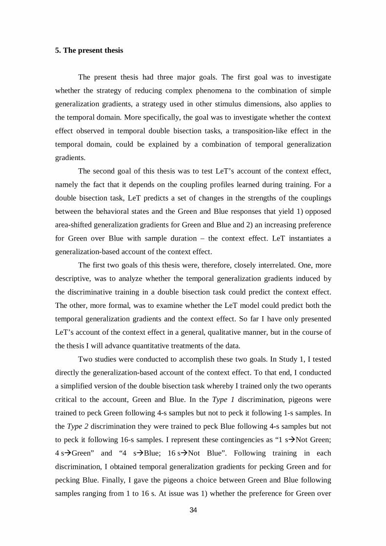
34
5. The present thesis
The present thesis had three major goals. The first goal was to investigate
whether the strategy of reducing complex phenomena to the combination of simple
generalization gradients, a strategy used in other stimulus dimensions, also applies to
the temporal domain. More specifically, the goal was to investigate whether the context
effect observed in temporal double bisection tasks, a transposition-like effect in the
temporal domain, could be explained by a combination of temporal generalization
gradients.
The second goal of this thesis was to test LeT’s account of the context effect,
namely the fact that it depends on the coupling profiles learned during training. For a
double bisection task, LeT predicts a set of changes in the strengths of the couplings
between the behavioral states and the Green and Blue responses that yield 1) opposed
area-shifted generalization gradients for Green and Blue and 2) an increasing preference
for Green over Blue with sample duration – the context effect. LeT instantiates a
generalization-based account of the context effect.
The first two goals of this thesis were, therefore, closely interrelated. One, more
descriptive, was to analyze whether the temporal generalization gradients induced by
the discriminative training in a double bisection task could predict the context effect.
The other, more formal, was to examine whether the LeT model could predict both the
temporal generalization gradients and the context effect. So far I have only presented
LeT’s account of the context effect in a general, qualitative manner, but in the course of
the thesis I will advance quantitative treatments of the data.
Two studies were conducted to accomplish these two goals. In Study 1, I tested
directly the generalization-based account of the context effect. To that end, I conducted
a simplified version of the double bisection task whereby I trained only the two operants
critical to the account, Green and Blue. In the Type 1 discrimination, pigeons were
trained to peck Green following 4-s samples but not to peck it following 1-s samples. In
the Type 2 discrimination they were trained to peck Blue following 4-s samples but not
to peck it following 16-s samples. I represent these contingencies as “1 sNot Green;
4 sGreen” and “4 sBlue; 16 sNot Blue”. Following training in each
discrimination, I obtained temporal generalization gradients for pecking Green and for
pecking Blue. Finally, I gave the pigeons a choice between Green and Blue following
samples ranging from 1 to 16 s. At issue was 1) whether the preference for Green over

35
Blue increased with sample duration – the context effect, 2) whether the two
generalization gradients predicted the choice data and 3) whether LeT accounted for
both the generalization gradients and the choice data.
In Study 2, I asked whether the strategy used in Study 1 with a simplified double
bisection task, would extend to the standard double bisection task. In other words, I
asked whether the gradients for Green and Blue obtained with the discriminations
“2 sRed; 6 sGreen” and “6 sBlue; 18 sYellow” also would predict the choice
between Green and Blue. Moreover, in this study I also examined the generalization
gradients and the choice functions for durations outside the training range. In all
previous studies with the double bisection task, including Study 1, the sample durations
used during testing were within the range of durations used during training.
The third goal of the present thesis was to deepen the study of the temporal
generalization gradients. Different from other stimulus dimensions, little attention has
been given to the study of generalization gradients in the temporal domain. Little is still
known about their features and the variables that affect them. Also following a strategy
used with other stimulus dimensions, my aim was to explore the effects of different
training protocols on the temporal generalization gradient. The first two studies of the
present thesis, although not primarily concerned with this issue, investigated temporal
generalization gradients following intradimensional training. Study 3, on the other hand,
examined the effects of interdimensional training on the temporal generalization
gradient. Only one study, conducted by Russell and Kirkpatrick (2007), approached the
topic and the results were not conclusive. Namely, it is not clear whether the obtained
non-flat gradient was present from the beginning of testing and, thus, was a result of the
training procedure, or only developed due to learning that took place during testing. In
Study 3 of the present thesis I replicated and extended Russell and Kirkpatrick (2007,
Experiment 1) to elucidate this issue.
Globally, in the present thesis I investigated whether phenomena found in other
stimulus dimensions are also found in the temporal domain. This type of analysis has
two important contributions. First, to increase our knowledge on the characteristics and
the processes involved in the temporal regulation of behavior. Second, to approximate
the temporal dimension to other stimulus dimensions and investigate whether two areas
that have been studied in parallel, namely the control of behavior by the temporal
properties of the stimuli and the control of behavior by other properties of the stimuli,
share features and processes.

36

37
CHAPTER II3
STUDY 1: TEMPORAL GENERALIZATION GRADIENTS AND THE CONTEXT EFFECT IN A SIMPLIFIED DOUBLE BISECTION TASK
3 This chapter is based on the publication:
Vieira de Castro, A. C., & Machado, A. (2012). The interaction of temporal generalization gradients predicts the context effect.
Journal of the Experimental Analysis of Behavior, 97, 263-279.

38

39
Abstract
In a temporal double bisection task, animals learn two discriminations. In the presence
of Red and Green keys, responses to Red are reinforced after 1-s samples and responses
to Green are reinforced after 4-s samples; in the presence of Blue and Yellow keys,
responses to Blue are reinforced after 4-s samples and responses to Yellow are
reinforced after 16-s samples. Subsequently, given a choice between Green and Blue,
the probability of choosing Green increases with the sample duration – the context
effect. In the present study we asked whether this effect could be predicted from the
stimulus generalization gradients induced by the two basic discriminations. Six pigeons
learned to peck Green following 4-s samples (S+) but not following 1-s samples (S-) and
to peck Red following 4-s samples (S+) but not following 16-s samples (S-). Temporal
generalization gradients for Green and Red were then obtained. Finally, the pigeons
were given a choice between Green and Red following sample durations ranging from 1
to 16 s. Results showed that a) the two generalization gradients had the minimum at the
S- duration, an intermediate value between the S- and the S+ durations, and the
maximum at the S+ as well as more extreme durations; b) on choice trials, preference for
Green over Red increased with sample duration, the context effect; and c) the two
generalization gradients predicted the average context effect well. The
Learning-to-Time model accounts for the major trends in the data.

40

41
1. Introduction
With the aim of contrasting some models of timing, Machado and Keen (1999)
developed the double bisection task, a modified version of one of the most well-known
procedures used to study timing in animals and humans – the temporal bisection task. In
a typical temporal bisection task, the subjects learn to discriminate between two samples
of different durations. For instance, a pigeon is presented with a sample light
illuminated for either 1 or 4 s and then with two comparison stimuli, a Red key and a
Green key. The pigeon receives food if it pecks Red following 1-s samples and Green
following 4-s samples. After the discrimination is acquired the animal is presented with
samples of intermediate durations and the preference for one of the keys, say, Green, is
assessed. It is commonly found that the proportion of responses to Green increases with
sample duration from about 0 to about 1, with the indifference point close to the
geometric mean of the two training durations (Catania, 1970; Church & Deluty, 1977;
Fetterman & Killen, 1991; Platt & Davis, 1983; Stubbs, 1968; for summaries, see
Gallistel, 1990; Richelle & Lejeune, 1980; Shettleworth, 1998).
In the double bisection procedure the animals learn not one but two temporal
discriminations, which we call Type 1 and Type 2. In the Type 1 discrimination they
learn to choose Red over Green after 1-s samples and Green over Red after 4-s samples.
In the Type 2 discrimination they learn to choose Blue over Yellow after 4-s samples
and Yellow over Blue after 16-s samples. Next, generalization tests are conducted in
which new pairs of comparisons are introduced following different sample durations. Of
critical importance to contrast timing models are the test trials on which Green and Blue
are presented together, for these two comparisons were reinforced following the same
sample duration of 4 s.
The typical result of these test trials is that preference for Green over Blue
increases with sample duration (e.g., Machado & Keen, 1999). This finding is called the
context effect because, even though the choices of Green and Blue were reinforced
following the same sample duration, the context in which such reinforcement occurred
differed. Choosing Green was reinforced in a context in which a shorter sample signaled
extinction for Green, whereas choosing Blue was reinforced in a context in which a
longer duration signaled extinction for Blue. As a series of studies using different
versions of the double bisection procedure have shown, the context effect is quite robust

42
and general (Arantes, 2008; Arantes & Machado, 2008; Machado & Arantes, 2006;
Machado & Keen, 1999; Machado & Pata, 2005; Oliveira & Machado, 2008, 2009).
The context effect is theoretically important because it differentiates timing
models. Consider the leading model, Scalar Expectancy Theory (SET; e.g., Church,
2003; Gibbon, 1977; Gibbon et al., 1984). According to SET’s standard account for
temporal bisection (e.g., Gibbon, 1981, 1991), the animal represents the reinforced
sample durations in distinct memory stores. Therefore, in the double bisection task, the
animal forms four stores, but only two are critical for the context effect, the store
representing 4-s samples and associated with the Green comparison and the store
representing 4-s samples associated with the Blue comparison. Moreover, according to
SET, the contents of each store depend exclusively on its corresponding sample
duration – they are context independent. Hence, the stores associated with Green and
Blue will have identical representations causing SET to predict that the preference for
Green over Blue will not vary with the sample duration. In short, because temporal
memories are assumed context-independent, SET fails to predict the context effect.
In contrast with SET, the Learning-to-Time or LeT model (Machado, 1997) or
its newer version (Machado et al., 2009) is a context-dependent timing model. It
assumes that, in a temporal discrimination task, the sample stimulus activates a set of
states serially such that, on the average, the active state at the end of the sample varies
directly with the sample duration (see also Killeen & Fetterman, 1988). Moreover, each
state is coupled with the comparison stimuli and the degree of the coupling changes
with reinforcement and extinction. Reinforcement strengthens and extinction weakens
the coupling between the active state and the chosen comparison. Finally, the
probability of choosing one or the other comparison depends on two factors, which state
is active at the end of the sample (a function of sample duration) and which of the two
couplings is stronger (a function of the reinforcement contingencies). Because the
couplings between the active states and the comparisons depend on the samples
durations and on which comparison is reinforced and which is extinguished following
each sample, the model is context-dependent.
Before we explain in greater detail how LeT accounts for the context effect, we
present a qualitative account of that effect that does not rely on a specific model. The
account conceives of a simultaneous discrimination as two successive discriminations
operating simultaneously. In the double bisection task, this means that pecking Green
and Blue are conceived of as operants controlled by two sample durations, an S+ and an

43
S-. For Green, the S+ and S- are the 4-s and 1-s samples, respectively; for Blue, the S+
and S- are the 4-s and 16-s samples, respectively. In addition, the account assumes that
choice between the two comparison stimuli may be predicted from the generalization
gradients induced by the discriminative training (Honig, 1962; Spence, 1937).
Machado and Pata (2005) suggested that the context effect could be the result of
a peak-shift-like phenomenon in the temporal domain. Peak shift refers to a shift in the
peak of a generalization gradient after intradimensional discrimination training, a shift
in the direction opposite to the negative stimulus (S-). If we assume that the effect of the
S- is to shift the peak of the generalization gradient away from S+ (Hanson, 1959; see
also Bloomfield, 1967; Purtle, 1973; Spence, 1937), then, in the double bisection task,
the gradient for Green will have its maximum at a value greater than 4 s, whereas the
gradient for Blue will have its maximum at a value less than 4 s. The net effect of these
two shifts is that the gradient for Blue will be above the gradient for Green for durations
less than 4 s, but the gradient for Green will be above the gradient for Blue for durations
greater than 4 s. The relative positions of the two gradients could explain why
preference for Green over Blue increases with sample duration.
A few studies have examined peak shift in post discrimination temporal
generalization gradients. Mellgren et al. (1983) with rats and Spetch and Cheng (1998)
with pigeons obtained generalization gradients resembling ramp functions (a high
response rate in the presence of the S+ and higher values, an intermediate response rate
for values between the S+ and the S-, and the same low response rate in the presence of
the S- and lower values); no peak shift was found. Siegel (1986) obtained peaked
gradients with rats but the peak remained at the S+. In Elsmore’s (1971) study, two
pigeons showed a peak shift effect and the other two responded approximately at the
same rate to the S+ and to the values on the far side of it. More recently, Russell and
Kirkpatrick (2007) found, with pigeons, gradients with a clear peak shift and gradients
that peaked at a duration away from the S+ in the direction opposite the S-, but did not
decrease significantly for the remaining durations. To summarize, the evidence for peak
shift in the temporal domain is mixed, with one study reporting positive evidence, three
studies reporting negative evidence and one other reporting, at least for some subjects,
positive evidence.
Peak shift, however, can be seen as a special case of the area shift phenomenon.
An area shift occurs when more than 50% of the area of the gradient lies on the side of
S+ opposite the S- (Rilling, 1977; see e.g. Cheng et al., 1997, for an area shift effect in

44
the spatial domain). It follows from the definition that whenever a peak shift occurs, an
area shift also occurs, but the reverse is not necessarily the case. In fact, whereas area
shift is reliably found in the temporal domain following intradimensional discrimination
training, including in all the studies reported above, peak shift does not always occur.
Hence, in what follows we focus our attention in the more general phenomenon of area
shift.
The area shift account of the context effect would work as follows. If we assume
that a) because the choice of Green is extinguished after 1-s samples, the area of the
gradient for Green will be shifted to the right (i.e., toward durations longer than 4 s); b)
because choice of Blue is extinguished after16-s samples, the area of the gradient for
Blue will be shifted to the left (i.e., toward durations shorter than 4 s); c) because of a)
and b), the generalization gradient for Green will be below that for Blue at 1 s,
approximately equal to it at 4 s, and above it at 16 s; d) if choice following a t-s sample
depends on the relative heights of the two gradients at t s, then the proportion of Green
choices should increase with sample duration, the context effect. According to this
account, the exact location of the peaks of the gradients is irrelevant.
The area shift hypothesis is consistent with how the LeT model accounts for the
context effect. We present the general argument qualitatively and defer until the
Discussion a more quantitative treatment (for additional details, see Machado et al.,
2009). Let S1, S4, and S16 represent the behavioral states most likely to be active at the
end of 1-s, 4-s and 16-s samples, respectively and “0”, “+” and “++” stand for weak,
moderate and strong couplings, respectively. Initially, the behavioral states are equally
coupled with the two critical comparisons, the Green and Blue keys, and the degree of
the coupling may be represented as “+”. During Type 1 trials, choices of Green will be
reinforced after 4-s samples and extinguished after 1-s samples. Hence, the coupling of
S4 with Green will increase to “++” but the coupling of S1 with Green will decrease to
“0”. Similarly, during Type 2 trials, choices of Blue will be reinforced after 4-s samples
and extinguished after 16-s samples and consequently the coupling of S4 with Blue will
increase to “++” but the coupling of S16 with Blue will decrease to “0”. Two
consequences follow from the coupling profiles acquired during training. First, if we
run generalization tests by presenting either the Green or the Blue key following
samples ranging from 1 s to 16 s, then we should obtain the two area-shifted
generalization gradients mentioned above, a gradient shifted to the right (Green) and a
gradient shifted to the left (Blue). Second, if the animal is given a choice between Green

45
and Blue following samples ranging from 1 s to 16 s, then it should prefer Blue
following 1-s samples, be indifferent following 4-s samples, and prefer Green following
16-s samples – the context effect.
The foregoing account also justifies the designation of a context effect.
Although the animal learns to respond to Green and Blue following the same 4-s
samples, the context in which such learning takes place differs: responses to Green are
extinguished following 1-s samples, whereas responses to Blue are extinguished
following 16-s samples. According to LeT, the difference in the learning context
explains why preference for Green over Blue increases with sample duration.
To summarize, the LeT model instantiates the area shift hypothesis. The
coupling profiles acquired during training induce area-shifted generalization gradients
which combined produce the context effect.
The main purpose of the present study was to test directly this generalization
based account of the context effect. To that end, we simplified the double bisection task
by retaining only the elements central to the account, the two operants and their
reinforcement contingencies – reinforcement after 4-s samples for both operants;
extinction after 1-s samples for one operant; and extinction after 16-s samples for the
other operant. Specifically, in the new task, the pigeons started by learning one of the
two basic discriminations, to peck A after 4-s samples, the S+, and not to peck A after
1-s samples, the S-. Then, we varied the sample duration from 1 to 16 s to obtain the
temporal generalization gradient for pecking A. Next, the pigeons learned the second
basic discrimination, to peck B after 4 s (S+), and not to peck B after 16 s (S-) and then
we varied the sample duration to obtain the gradient for pecking B. Finally, we
presented the pigeons with samples ranging from 1 to 16 s and gave them a choice
between the two operants, peck A and peck B. According to our hypothesis, the
preference of A over B should increase with sample duration, and, in addition, the two
generalization gradients, with their areas shifted in opposite directions, should predict
the preference data.
One potential difficulty with the task described above is that it involves
successive choice during the basic discriminations (e.g., peck A following 4-s samples;
do not peck A following 1-s samples), but simultaneous choice during the final test
phase (peck A or B). The novelty of simultaneous choice during the final test phase
could mask the effects of the generalization gradients induced by the two basic
discriminations. To eliminate this potential difficulty, we introduced a “dummy”

46
alternative during the basic discriminations. Specifically, after 1-s and 4-s samples, the
pigeon was given a choice between pecking A (e.g., a Green key) and pecking a key
with a vertical bar. Choice of A was reinforced after the 4-s samples, but not after the
1-s samples, and choice of the vertical bar was never reinforced. Similarly, after 4-s and
16-s samples, the pigeon was given a choice between pecking B (e.g., a Red key) and
pecking a key with a vertical bar. Choice of B was reinforced after the 4-s samples, but
not after the 16-s samples, and again choice of the vertical bar was never reinforced.
The “dummy” alternative gave the pigeons experience with simultaneous choice from
the beginning of the experiment.
2. Method
2.1. Subjects
Six adult pigeons (Columba livia) participated in the experiment. The birds had
previous experience with the time-left procedure, but not with matching-to-sample
tasks. They were maintained at 80% of their free-feeding body weights throughout the
experiment and were housed in individual home cages with water and grit continuously
available. A 13:11 h light/dark cycle, beginning at 8:00 am, was in effect in the pigeon
colony.
2.2. Apparatus
Three identical Lehigh Valley® operant chambers were used. Each chamber was
34-cm high, 35-cm long and 31-cm wide. The walls and ceiling were made of
aluminum and the floor was wire mesh. The response panel contained three circular
keys, 2.5 cm in diameter, arranged in a horizontal row, 22.5 cm above the floor, and
9 cm apart, center to center. The keys could be illuminated with yellow, green and red
lights and with a vertical white bar on a dark background. On the back wall of the
chamber, 4 cm below the ceiling, a 7.5-W houselight provided general illumination.
Reinforcement consisted of mixed grain delivered by a hopper that was accessible
through a 6×5-cm opening, centered on the response panel 8.5 cm above the floor. A
7.5-W white light illuminated the opening whenever a reinforcer was available. An
outer box enclosed the operant chamber. The box was equipped with a ventilation fan

47
that circulated air through the chamber and provided masking noise. A personal
computer controlled all experimental events and recorded the data.
2.3. Procedure
The pigeons learned two temporal discriminations, 1 s vs. 4 s and 4 s vs. 16 s,
referred to as Type 1 and Type 2, respectively. Half of the birds learned the Type 1
discrimination first and the Type 2 discrimination next, whereas the other half learned
the discriminations in the opposite order. For three pigeons (P170, P178, and P841) a
Green key was associated with the 4-s samples from Type 1 trials and a Red key was
associated with the 4-s samples from the Type 2 trials; for the other three pigeons, the
reverse assignment was in effect. However, for clarity we describe the procedure and
the experimental results as if all of the birds had learned the Type 1 discrimination first
and had the Green key assigned to the 4-s sample of the Type 1 discrimination.
Table 3 summarizes the procedure. It comprised three phases, one in which only
the Type 1 discrimination was trained, another in which only the Type 2 discrimination
was trained, and yet another in which both Type 1 and Type 2 discriminations were
trained. In addition, each phase comprised three conditions, Training, during which the
discrimination was learned and all correct choices were reinforced, Pretesting, during
which some correct choices were extinguished to adapt the pigeons to the intermittent
reinforcement that would be in effect during the next condition, and Testing, during
which new sample durations were introduced to obtain the generalization gradients
(Phases 1 and 2), or new sample durations and a new pair of choice keys, Green and
Red, were introduced to examine the context effect (Phase 3).

48
Table 3. Comparison Stimuli, Sample duration, and the number of reinforced and non-reinforced trials per
session for each Phase and Condition of the experiment. N+ means that N trials per session were
reinforced (provided the choice was correct) and N- means that N trials per session were in extinction.
Phase 1
The general structure of a Type 1 Training Condition trial was as follows. After a
dark, 20-s ITI, the houselight was turned on and the center key was illuminated with
yellow light. After the sample duration elapsed (1 s or 4 s) the center keylight was
turned off and the side keys were illuminated, one with a green light and the other with
a white vertical bar on a dark background. The two side keys remained illuminated for
at least 6 s. If the S+, 4-s sample had been presented, the first peck at a choice key after
6 s turned all keylights and the houselight off, and if the response was correct (pecking
Phase Condition Comparison Stimuli
Sample duration (s)
1 2 4 8 16
Type 1 Training Bar Green 30- 30+
Pretesting Bar Green 30- 24+,6-
Testing Bar Green 30- 2- 24+ 2- 2- Type 2 Training Bar Red 30+ 30-
Pretesting Bar Red 24+,6- 30-
Testing Bar Red 2- 2- 24+ 2- 30-
Type 1 + Type 2 (Combined)
Training Bar Green 20- 20+
Bar Red 20+ 20-
Pretesting Bar Green 20- 14+,6-
Bar Red 14+,6- 20-
Testing Bar Green 20- 14+
Bar Red 14+ 20-
Green* Red 6- 6-
Green* Red 4- 4- 4-
Green** Red 6- 6-
Green** Red 4- 4- 4-
*For pigeons P890, P948, P178, and P841 **For pigeons P170 and PG12

49
Green), it activated the food hopper. The hopper duration varied across birds from 3 s to
9 s in order to maintain body weight with minimal extra session feeding. After food, the
ITI followed. If the response was incorrect (pecking the vertical bar), the ITI started
immediately and the trial was repeated. If the bird made three consecutive errors, only
the Green key was presented (correction procedure). If the S-, 1-s sample had been
presented, the side keys and the houselight were turned off after the 6-s period
regardless of the animal’s behavior and then the ITI started.
Learning was assessed by the relative response rate during the 6-s choice period,
that is, by the discrimination ratio “#S+/(# S+ + # S-)”, where #S+ is the total number of
responses to Green after the 4-s samples, and #S- is the total number of responses to
Green after the 1-s samples. Initially, the learning criterion was set at a discrimination
ratio of .85 or above, excluding repeated trials, for 5 consecutive sessions. For some
subjects, the criterion had to be reduced to .80 because the initial criterion proved to be
too hard to reach.
Sessions 1 to 12 comprised 60 trials, 30 with the S+ and 30 with the S- (see first
row of Table 3). Within each set of 30 trials, 15 had Green on the left key and 15 had
Green on the right key. However, as some birds continued to peck Green during the S-
trials, in subsequent sessions we increased the proportion of S- trials: 20 S+ and 40 S-
trials for pigeons P170, P178, P890, and PG12, and 16 S+ and 44 S- trials for pigeons
P841 and P948. For the last two pigeons we also reduced to 3 s the duration of the
choice period in order to make their choice responses more contiguous with
reinforcement and extinction. Before advancing to the next condition, though, all
pigeons returned to the original session structure with 30 S+ and 30 S- trials and a 6-s
choice period. The Training Condition lasted 42 sessions on average (range: 32 to 69).
In the Pretesting Condition (see second row of Table 3), extinction trials were
introduced. In addition to not ending with food, even when a choice was correct,
extinction trials also were not repeated when the choice was incorrect. Sessions
comprised 60 trials, 30 S+ (24 reinforced and 6 unreinforced, 12 and 3 for each left/right
assignment, respectively) and 30 S- (15 for each left/right assignment). Pretesting lasted
until the learning criterion was met (M=7 sessions; range: 5 to 12).
In the Testing Condition (see third row of Table 3), each session comprised 60
trials, 24 S+ and 30 S- (12 and 15 for each left/right assignment, respectively) and 6 test
trials. On test trials the sample duration equaled 2, 8 or 16 s, and each sample was
presented twice per session (once for each left/right assignment). If during any test

50
session a bird’s discrimination ratio decreased by more than .05 from its criterion (either
.85 or .80), the bird was returned to training for at least 2 sessions and until its
performance met the criterion again. Testing continued until 10 test sessions were
completed (M=12 sessions; range: 10 to 19).
Phase 2
After the pigeons completed the three conditions of Phase 1, they were exposed
to exactly the same conditions but with the Type 2 discrimination (see Table 3).
Training lasted from 16 to 53 sessions (M=30), Pretesting from 5 to 17 (M=7) and
Testing from 12 to 26 (M=15).
Phase 3
Initially, the Type 1 and Type 2 discriminations alternated across sessions for a
minimum of 5 sessions and until the pigeons reached the criterion. Next, both
discriminations were presented within the same session (see Table 3, “Type 1 +
Type 2”). Each session comprised 80 trials, 40 of Type 1 and 40 of Type 2. For each
type, there were 20 S+ and 20 S- trials (10 for each left/right assignment). Training
lasted from 6 to 31 sessions (M=16).
During the Pretesting Condition, the session structure remained the same except
that a few S+ trials were conducted in extinction (see Table 3). Pretesting lasted from 5
to 18 sessions (M=7).
During the Testing Condition, each session comprised 68 training trials and 12
test trials for a total of 80 trials. During the test trials, Green and Red were presented
together for the first time. In addition, the sample duration on test trials equaled 1 s or
16 s during the first 6 sessions and 2 s, 4 s or 8 s during the next 9 sessions (see Table 3,
3rd and 4th rows from bottom). Due to a programming error, for pigeons P170 and PG12,
the sample durations equaled 1 s and 8 s during the first 6 sessions and 2 s, 4 s and 16 s
during the next 9 sessions (Table 3, last two rows). Each test trial was presented six
times per session during the first 6 sessions, and four times per session during the last 9
sessions.
If during any test session a bird’s discrimination ratio for Type 1 or Type 2 trials
decreased by more than .05 from its current criterion (either .80 or .85), the bird

51
returned to training for at least 2 sessions and until its performance recovered. However,
for pigeons P948 and P841, testing disrupted the Type 1 discrimination to such extent
that the criterion had to be lowered. Pigeon P948 recovered partly and completed the
tests with the criterion set at .75 for the Type 1 discrimination; for Type 2 trials, the
criterion was maintained at .80. Pigeon P841 did not recover the Type 1 discrimination,
even after 20 sessions of Training and Pretesting. Because its ratio for Type 2 trials
remained above .80 and the ratio for Type 1 trials stabilized around .65, testing was
resumed. The Testing Condition, with intercalated training sessions when required,
lasted from 15 to 42 sessions across birds (M=22).
3. Results
Training
By the tenth session of training five of the six pigeons were rarely pecking the
key with the vertical bar (fewer than 2 pecks per session on average); P841 was the
exception, for this pigeon maintained some responding to the vertical bar throughout the
experiment (from 4.5 to 30.8 pecks per session).
All subjects learned the two basic discriminations. They required a similar
number of sessions to learn the Type 1 and Type 2 discriminations (M=35 and 37
sessions, respectively, t(5)=0.29, ns). And though the discrimination learned in the
second place (Type 1 for half of the pigeons and Type 2 for the other half) required
fewer sessions than the discrimination learned in the first place (M=30 and 42,
respectively), the difference was not statistically significant (t(5)=1.83, p=.13). During
the last five training sessions, the discrimination ratio averaged .93 on Type 1 trials
(range: .84 – .99) and .92 on Type 2 trials (range: .89 – .97). When the two
discriminations were combined into the same session, the overall discrimination ratio
averaged .90 (range: .82 - .99).
The total number of sessions required to learn the two discriminations (i.e.,
Type 1 alone + Type 2 alone + Types 1 and 2 combined) ranged from 93 to 158
(M=118). This number is significantly higher than the number obtained in previous
studies with a simultaneous double bisection procedure (e.g., 29 to 34 in Machado &
Keen, 1999; 27 to 65 in Machado & Pata, 2005; 26 to 45 in Machado & Arantes, 2006;
28 to 68 in Oliveira & Machado, 2008; and 26 to 38 in Oliveira & Machado, 2009).

52
However, the number is close to that obtained by Arantes (2008) with a successive
double bisection procedure (M=103, range: 51 - 133). These results (see also Arantes &
Grace, 2008) show that simultaneous double bisection tasks are easier to learn than
successive ones, presumably because learning to not respond following an S- is easier if
the same S- is an S+ for responding on another key.
Stimulus Generalization Testing
Figure 12 shows the stimulus generalization gradients for the two temporal
discriminations. The response rate on the Green or Red keys during the 6-s choice
period is plotted against sample duration. All pigeons exhibited similar generalization
gradients: Response rate was lowest at the S-, intermediate between the S- and the S+,
and highest at the S+ and durations further away from the S-. For pigeon P890, the
gradient for Type 2 trials decreased for the shortest sample duration of 1 s.
Figure 12. Generalization gradients obtained after the Type 1 (S+=4s, S-=1s) and Type 2 (S+=4 s, S-=16 s)
discriminations. Note the logarithmic scale on the x-axis.
Signal duration (s)
1 2 4 8 16012345 P170
1 2 4 8 16
Res
pons
es p
er se
c
0
1
2
3 P178
1 2 4 8 1601234 P841
1 2 4 8 1601234 P890
1 2 4 8 160
1
2
3 P948
1 2 4 8 160
1
2
3
PG12
S- = 1S- = 16
S+
Sample duration (s)

53
Figure 13 shows that the average gradient was similar for the two
discriminations. Response rate increased from the S- to the S+ and then it remained high
(Type 1) or decreased slightly (Type 2). A two-way repeated-measures ANOVA, with
sample duration and type of discrimination as factors revealed significant effects of
sample duration [F(4, 20)=38.95, p<.001], type of discrimination [F(1, 5)=15.10,
p<.05], and their interaction [F(4, 20)=59.72, p<.001].
To analyze the symmetry of the two generalization gradients, we reflected the
curve for Type 2 trials around the line t=4. The bottom panel of Figure 13 shows the
result. The (reflected) gradient for Type 2 trials was below the gradient for Type 1 trials,
particularly at the geometric means of the training durations (i.e., t=2 s for Type 1 and
t=8 s for Type 2) and at the extreme durations on the opposite side of S- (t=16 s for
Type 1 and t=1 s for Type 2). A two-way, repeated-measures ANOVA with sample
duration and type of discrimination as factors revealed that all effects were significant
(type of discrimination, F(1, 5)=15.10, p<.05, sample duration, F(4, 20)=68.66, p<.001,
and their interaction F(4, 20)=6.17, p<.005).
Figure 13. Top panel. Average generalization gradients obtained after the Type 1 (S+=4 s, S-=1 s) and
Type 2 (S+=4s, S-=16s) discriminations. Bottom panel. The gradient for Type 2 trials is reflected along the
vertical line t=4 (the inverted x-axis shows the original sample durations). The bars show the SEM. Note
the logarithmic scale on the x-axis.
S- = 1S- = 16
S+
1 2 4 8 16
Res
p. p
er se
c
0
1
2
3
4
1 2 4 8 16
Res
p. p
er se
c
0
1
2
3
4
Signal duration (s)16 8 4 2 1
Sample duration (s)

54
Paired t-tests conducted for the t=2 s, t=8 s and t=16 s samples (defined by the
Type 1 discrimination in the bottom panel of Figure 13) revealed a significant difference
between response rate on t=2 s and t=16 s [t(5)=5.42, p<.05 and t(5)=3.66, p<.05,
respectively]; on t=8 s the difference approached significance [t(5)=2.27, p=.07].
Stimulus-Response Generalization Testing
The data analysis from the choice tests addresses an important question: Does
the context effect hold even when only two responses are reinforced, that is, when
pecking Green and Red are reinforced following 4-s samples but not following 1-s and
16-s samples, respectively? Figure 14 shows the individual and average results. The
filled circles show that the preference for Green – defined by the ratio between the total
number of responses to Green and the total number of responses to Green plus Red –
tended to increase with sample duration. A repeated-measures ANOVA revealed a
significant effect of sample duration, F(4,20)=13.79, p<.001.
The filled circles in the bottom panel show that, on the average, preference for
Green increased monotonically from about .10 to about .70, thus reproducing the
context effect previously found with other variants of the double bisection task
(compare Figures 2 and 5; see also Arantes, 2008; Arantes & Machado, 2008; Machado
& Arantes, 2006; Machado & Keen, 1999; Machado & Pata, 2005; Oliveira
& Machado, 2008, 2009).
The individual curves show some variability across birds. Pigeons P890, P948
and P178 displayed steep, monotonically increasing preference functions; pigeon P841
also presented a monotonically increasing function, but it never exceeded .50; for
pigeons PG12 and P170, preference for Green also tended to increase with sample
duration, although not monotonically. Three subjects revealed a strong overall bias for
one comparison, Green in the case of PG12 and Red in the case of P170 and P841.
The causes of the individual differences in the strength of the context effect
remain unclear. On the one hand, the relatively weaker effect revealed by pigeon P841
could be due to its poor discrimination between the 1-s and 4-s samples during Phase 3,
but the same cannot be said of pigeons P170 and PG12 because their discrimination
ratios never fell below .80. On the other hand, pigeons P170 and PG12 started the
choice test with sample durations of 1 s and 8 s, whereas the remaining pigeons started

55
them with sample durations of 1 s and 16 s, but it is unclear how this difference could
explain the differences in the strength of the context effect.
Figure 14. The top panels show the individual functions relating preference for Green over Red to sample
duration. Filled and unfilled circles correspond to different measures of preference, relative response rate
or “all-or-none”. The bottom panel shows the average results. The vertical bars show the SEM. Note the
logarithmic scale on the x-axis.
Another potential source of the individual differences may be the number of
choice trials on which the pigeon pecked neither the Green nor the Red keys. Table 4
shows the number of these “empty” trials, out of 36, for each pigeon and sample
duration. The number of empty trials was particularly high following the 8-s and 16-s
Avg
1 2 4 8 160.0
0.5
1.0 P170
P178
P841
P890
P948
PG12
1 2 4 8 160.0
0.5
1.0
1 2 4 8 160.0
0.5
1.0
1 2 4 8 160.0
0.5
1.0
1 2 4 8 16
Pref
eren
ce fo
r Gre
en o
ver R
ed
0.0
0.5
1.0
1 2 4 8 160.0
0.5
1.0
Signal duration (s)1 2 4 8 16
Pref
. for
G o
ver R
0.0
0.5
1.0
Rel. rateAll-or-none
Sample duration (s)

56
samples. However, there was no clear relation between that number and the preference
for Green. Consider the 16-s samples: Of the three pigeons that showed a strong
preference for Green, two had a large number of empty trials (P890 and P178) but one
had only one empty trial (P948). The case was similar following 1-s samples.
Spearman’s rank-order correlations between the number of empty trials and the
preference for Green were not statistically significant (see Table 4, bottom lines).
Table 4. Number of empty trials (out of 36) following each sample duration. rs is Spearman’s rank-order
correlation between the number of empty trials and the preference for Green. p is the corresponding p-
value under H0.
Although variation in the number of empty trials does not seem to account for
the differences in the context effect, the large number of empty trials following some
sample durations raises an interpretative problem related to the measurement of
preference. Consider the data for pigeon P170. The 33 empty trials following the 16-s
samples mean that the pigeon responded on 3 trials only. On two of them, it chose
Green, and on one of them it chose Red, which suggests a preference for Green.
However, preference for Green measured by relative response rate was only .27 (see
Figure 14) because response rate on Red was higher than on Green. Differences in
response rate may have contaminated the preference measure.
This difficulty suggested a second way to measure preference. For each sample,
we counted the number of trials on which the pigeon pecked Green at least once (even
if it also pecked Red) and then divided it by the total number of trials on which the
pigeon pecked at least one key. This “all-or-none” preference measure is not affected by
differences in response rate.
Sample duration Pigeon 1 2 4 8 16 P170 0 0 1 13 33 P178 21 7 0 11 22 P841 0 0 0 7 4 P890 18 24 1 26 30 P948 2 1 0 6 1 PG12 7 10 0 20 27 Avg 8 7 0 14 20
rs -.03 .32 .42 .43 -.20 p .48 .27 .20 .20 .35

57
The unfilled circles in Figure 14 show the “all-or-none” measure. It is clear that
both preference measures yielded similar results. The correlations between them were
strong for four pigeons (.91≤r2≤.99 for P178, P841, P890, and P948), and moderate for
the remaining two (.60≤r2≤.75). The averages of the two measures (see bottom panel)
were positively correlated (r2=.97). We conclude that, with few exceptions, the two
measures of preference were consistent and, therefore, that relative response rate is a
reliable measure of preference in the present task.
Predicting Preference Functions from Stimulus Generalization Gradients
The major goal of the present study was to assess how well the context effect
found in double bisection tasks could be predicted from the stimulus generalization
gradients. To that end we carried out the following analysis. For each pigeon and
sample duration, we used the response rates from Phases 1 and 2 displayed in Figure 12
to compute the predicted preference for Green. Specifically, we divided the absolute
response rate to Green by the sum of the absolute response rates to Green and Red.
Finally, we plotted the preference function predicted from the generalization gradients
and compared it with the preference function obtained during the choice test. Figure 15
shows the results.
All six predicted functions (unfilled circles) expressed the context effect: The
preference for Green increased monotonically with sample duration. In addition, for
pigeons P890, P948, and P178, the predicted and obtained functions were similar
(r2=.93, .90, and .85, respectively); for pigeon P841 the two functions differed
appreciably at 8- and 16-s sample durations (r2=.81); and for pigeons P170 and PG12,
they differed considerably (r2=.54 and .27, respectively). Interestingly, the pigeons that
showed the greatest overlap between the predicted and the obtained preference
functions also showed the strongest context effect.
The average of the predicted functions (see bottom panel) increased
monotonically from about .10 to .90. Although more extreme than the average of the
obtained preference functions, it had approximately the same shape. The two average
functions were strongly correlated (r2=.93).

58
Figure 15. Filled circles show the preference for Green obtained in the Testing Condition of Phase 3 with
samples ranging from 1 to 16 seconds and Green and Red as comparisons. The unfilled circles show the
preference for Green predicted from the gradients obtained during the stimulus generalization tests of
Phases 1 and 2. The vertical bars show the SEM. Note the logarithmic scale on the x-axis.
4. Discussion
Six pigeons were exposed to a simplified version of the temporal double
bisection procedure. On Type 1 trials they learned to peck a Green key following 4-s
samples but not to peck it following 1-s samples; on Type 2 trials they learned to peck a
Red key following 4-s samples but not following 16-s samples. After each
discrimination was learned, a stimulus generalization gradient was obtained by varying
Avg
1 2 4 8 160.0
0.5
1.0 P170
P178
P841
P890
P948
PG12
1 2 4 8 160.0
0.5
1.0
1 2 4 8 160.0
0.5
1.0
1 2 4 8 160.0
0.5
1.0
1 2 4 8 16
Pref
eren
ce fo
r Gre
en o
ver R
ed
0.0
0.5
1.0
1 2 4 8 160.0
0.5
1.0
Signal duration (s)1 2 4 8 16
Pref
. for
G o
ver R
0.0
0.5
1.0
Obs.Pred.
Sample duration (s) (s) (s)

59
sample duration from 1 to 16 s. Next, the two trial types were included in the same
session and a stimulus-response generalization test was conducted in which the samples
ranged from 1 to 16 s and the comparison stimuli were the Green and Red keys. The
study had two interrelated goals, to investigate whether the two temporal generalization
gradients could predict the context effect that was expected to occur during the choice
trials, and to determine whether the generalization gradients as well as the context effect
were consistent with the LeT model.
The choice test showed that, for four out of six pigeons, preference for Green
over Red increased monotonically with the sample duration (Figure 14). For the other
two, the effect was weaker but the overall positive trend was observed. The context
effect was obtained regardless of whether preference was assessed by relative response
rate or by an “all-or-none” measure that is not influenced by differences in response rate
between the two keys. And in spite of considerable procedural changes, the magnitude
of the average effect was similar to that obtained in previous studies. Replicating the
context effect in a situation where only two responses were reinforced opened the
possibility to test a generalization based account of it.
The results showed that the average context effect could be predicted from the
generalization gradients. However, the accuracy of the predictions varied across
pigeons. For three of them (see Figure 15, left panels), the generalization gradients
predicted well not only the positive trend, but also the specific values of the preference
functions; for the other three, the gradients predicted well only the positive trend of the
preference functions (Figure 15, right panels). The mismatches between the predicted
and observed function values revealed that the generalization gradients tended to
overestimate the strength of the context effect (cf. the slopes of the two functions in the
right panels of Figure 15).
The reasons for the mismatches remain unclear. They could stem from
generalization decrement because the stimulus conditions during the training and
generalization trials (i.e., only one of the keys, Green or Red, was present) differed from
the stimulus conditions during the choice trials (i.e., both the Green and Red keys were
present). Furthermore, some pigeons may have learned that the distinctive combination
of Green and Red keys signaled extinction and, as a consequence, they did not respond
on a large proportion of choice trials (Table 4). (The large number of empty trials,
particularly following the extreme sample durations of 1 s and 16 s, may have been
caused also by the preceding stimulus generalization tests, which also were conducted

60
in extinction.). A small number of non-empty trials could have distorted the measure of
preference. However, note that there was no significant correlation between the number
of empty trials and the degree of preference for the Green or Red keys. Also, how well
the generalization gradients predicted the context effect did not seem to depend on how
much the basic discriminations were disrupted during testing. In any event, the nuisance
of empty trials may be reduced in future studies by using a two-group design, with only
one group exposed to generalization tests, and by using choice tests with partial but
non-differential reinforcement.
To account for the context effect in terms of generalization gradients, we
advanced one qualitative account relying on area shift, and one quantitative account
based on the LeT model. We analyze them in this order.
Qualitative account
According to the area shift account, gradients obtained after intradimensional
training are asymmetrical, displaying a higher number of responses in the side of S+
opposite the S-. Then, the area of the generalization gradient on Type 1 trials should be
shifted toward durations longer than 4 s, and the area of the generalization gradient on
Type 2 trials should be shifted toward durations shorter than 4 s.
The generalization gradients obtained in Phases 1 and 2 matched these
predictions. All 12 gradients showed an area shift effect. The gradient produced by
pigeon P890 during Type 2 trials (see the top right panel in Figure 12), in contrast with
the other gradients, showed a clear reduction in response rate for stimulus values moved
away from the S+ in the direction opposite to the S-. It is conceivable that a closer
spacing of the test stimuli in the vicinity of S+ (4 s) might have revealed a peak around
t=3 s. In the other 11 gradients, response rate increased as the stimulus duration changed
from the S- to the S+, and then it remained high as the stimulus duration continued to
change past the S+ (see Figures 12 and 13). The shape of these gradients resembles a
ramp function, with a low response rate at the S-, an intermediate response rate between
the S- and the S+, and a high response rate at and past the S+. Because the gradients
obtained in the present experiment revealed an area shift effect and could predict the
context effect, we conclude that the area shift account works well in explaining our
findings.

61
The “opposed” generalization gradients displayed in Figure 12 and in the top
panel of Figure 13 are similar to the gradients obtained by Boneau and Honig (1964).
These authors were the first to examine generalization gradients based upon conditional
discrimination training. As in the present study, their pigeons learned two conditional
discriminations. When the response key was illuminated with a 550-nm light, a white
vertical bar added to the key was the S+ and the absence of the bar was the S-; when the
response key was illuminated with 570-nm light, the contingencies were reversed, the
S+ and S- were the absence and presence of the bar, respectively. During generalization
tests, the authors varied the wavelength of the light from 540 to 580 nm with either the
bar present or with the bar absent. When the bar was present, the generalization gradient
was high at 540 and 550 nm and low at 570 and 580. When the bar was absent, the
generalization gradient was low at 540 and 550 nm, high at 570 nm, and low again at
580 nm. If we replace wavelength with sample duration and the presence/absence of
the bar with Green/Red keylight color, then we can conceive of the present study as
extending Boneau and Honig’s (1964) findings to the timing domain. In both studies,
the areas of the two gradients shifted in opposite directions and no peak shift effect was
observed.
A quantitative (and integrative) account: the LeT model
To see how well the LeT model reproduces the major trends in the data, we ran a
simulation of the entire experiment, following the same phases and conditions as the
pigeons, and for a similar number of sessions. Throughout, the model parameters
remained constant and their values were similar to those used in previous studies
(Machado et al., 2009).
The model behaves as follows. Consider a Type 1 training trial. During the
sample, the behavioral states are activated serially – first state 1, then state 2, etc. Each
state remains active for seconds, with sampled at trial onset from a normal
distribution with mean s and standard deviation s. At the end of the sample
one state is active, say, state n*. This state is coupled with the operant response (e.g.,
Green) and the degree of the coupling, always between 0 and 1, is represented by the
variable WG(n*). When there is only one key, as during training and generalization

62
trials4, WG(n*) yields the probability of emitting a response. (To keep the simulation
simple and focus on the shape of the predicted curves, we did not attempt to model
absolute response rate.) When a response occurs, WG(n*) changes, increasing if the
response is reinforced (i.e., WG(n*)=(1-WG(n*)) and decreasing if the response is
extinguished (i.e., WG(n*)=-WG(n*)), where =0.2 and =0.04 are learning
parameters.
In the present simulation, the coupling of each state was initialized at 0.8 (i.e.,
WG(n)=0.8, for n=1, 2, 3,…) ensuring that, during the first session, a response on the
Green key was very likely to happen on each trial. After 40 sessions, with reinforcement
following 4-s samples and extinction following 1-s samples, the WG(n) values changed
and the result is the curve with filled circles displayed in the top panel of Figure 165.
The early states, active mostly after the 1-s samples, lost their coupling with Green, but
subsequent states, active mostly after the 4-s samples, had their coupling strengthened.
The remaining states, almost never active during Type 1 trials, retained their initial
coupling of 0.8.
The simulation details for Type 2 trials were the same except that a different
vector, WR(n), coupled the states with the Red key. The curve with open circles shows
how the WR(n) values changed with training from their initial value of 0.8. The early
states, active mostly after the 4-s samples, either retained or strengthened their
couplings with Red, whereas the states active mostly after the 16-s samples lost most of
their coupling.
The middle panel shows the generalization gradients. Nothing in the model
changed from training to testing. These gradients reflect the coupling strengths (W)
resulting from training. To illustrate, consider the curve for Type 1 trials (filled circles).
The gradient at 1 s is close to zero because after 1-s samples a) the initial states (n=1
and 2) are the most likely to be active, and b) as the top panel shows, those states have
close-to-zero couplings with Green. The generalization gradient reaches its maximum at
4 s because after 4-s samples the most active states are the intermediate states (n=3 to
6), which are strongly coupled with Green (see top panel). The response probability at
2 s occurs because the states most likely to be active after the 2-s samples, States 2 4 All training and generalization trials included also a key with a vertical bar. However, because pecks on that key were never
reinforced, and after the first few sessions the pigeons rarely pecked at it, the model ignores it.
5 The contribution of the Pretesting Condition (partial reinforcement) to the coupling strengths (W) is negligible, thus when the
animal advances to testing the response probabilities, yielded by WG and WR, would basically be the same.

63
and 3, have weak and strong couplings with Green, respectively; the net effect is an
intermediate response probability. Finally, the gradient decreases slightly after 4s
because the couplings of later states (n>6), the states most likely to be active at the end
of 8-s and 16-s samples, are not as strong as the coupling of the intermediate states.
Figure 16. Results from the simulation of the LeT model (Machado et al., 2009). Top panel. Strength of
the couplings between the behavioral states and the operant responses, Green and Red, at the end of the
Training Conditions of Phases 1 and 2 (see Table 2). Middle panel. Generalization gradients obtained
during the Testing Conditions of Phases 1 and 2. Bottom panel. Preference for Green over Red obtained
during the Testing Condition of Phase 3. Note the logarithmic scale on the x-axis in the middle and
bottom panels.
Signal duration (s)1 2 4 8 16
Res
p. p
roba
bilit
y
0.0
0.5
1.0 S- = 16 S- = 1
S+
Signal duration (s)1 2 4 8 16Pr
efer
ence
for G
reen
0.0
0.5
1.0
State (n)0 10 20 30 40C
oupl
ing
stre
ngth
(W)
0.0
0.5
1.0
WGWR
Sample duration (s)
Sample duration (s)
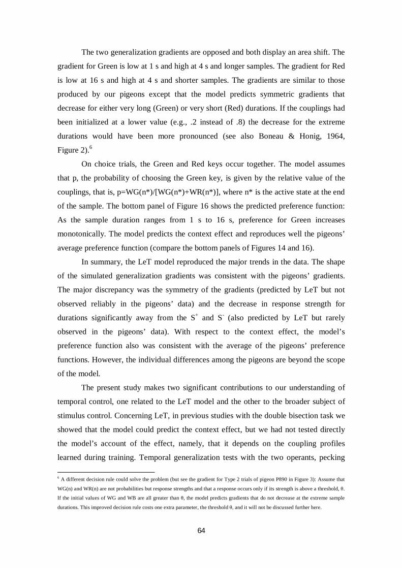
64
The two generalization gradients are opposed and both display an area shift. The
gradient for Green is low at 1 s and high at 4 s and longer samples. The gradient for Red
is low at 16 s and high at 4 s and shorter samples. The gradients are similar to those
produced by our pigeons except that the model predicts symmetric gradients that
decrease for either very long (Green) or very short (Red) durations. If the couplings had
been initialized at a lower value (e.g., .2 instead of .8) the decrease for the extreme
durations would have been more pronounced (see also Boneau & Honig, 1964,
Figure 2).6
On choice trials, the Green and Red keys occur together. The model assumes
that p, the probability of choosing the Green key, is given by the relative value of the
couplings, that is, p=WG(n*)/[WG(n*)+WR(n*)], where n* is the active state at the end
of the sample. The bottom panel of Figure 16 shows the predicted preference function:
As the sample duration ranges from 1 s to 16 s, preference for Green increases
monotonically. The model predicts the context effect and reproduces well the pigeons’
average preference function (compare the bottom panels of Figures 14 and 16).
In summary, the LeT model reproduced the major trends in the data. The shape
of the simulated generalization gradients was consistent with the pigeons’ gradients.
The major discrepancy was the symmetry of the gradients (predicted by LeT but not
observed reliably in the pigeons’ data) and the decrease in response strength for
durations significantly away from the S+ and S- (also predicted by LeT but rarely
observed in the pigeons’ data). With respect to the context effect, the model’s
preference function also was consistent with the average of the pigeons’ preference
functions. However, the individual differences among the pigeons are beyond the scope
of the model.
The present study makes two significant contributions to our understanding of
temporal control, one related to the LeT model and the other to the broader subject of
stimulus control. Concerning LeT, in previous studies with the double bisection task we
showed that the model could predict the context effect, but we had not tested directly
the model’s account of the effect, namely, that it depends on the coupling profiles
learned during training. Temporal generalization tests with the two operants, pecking
6 A different decision rule could solve the problem (but see the gradient for Type 2 trials of pigeon P890 in Figure 3): Assume that
WG(n) and WR(n) are not probabilities but response strengths and that a response occurs only if its strength is above a threshold, θ.
If the initial values of WG and WB are all greater than θ, the model predicts gradients that do not decrease at the extreme sample
durations. This improved decision rule costs one extra parameter, the threshold θ, and it will not be discussed further here.

65
Green and pecking Red, are one way of revealing these coupling profiles and thereby of
testing one of the model’s hidden components. Because in LeT choice proportions
depend on the coupling profiles, the latter are more fundamental than the former.
Putting to test the model’s assumptions about the coupling profiles is a significant
advance over testing only the model’s predictions about choice proportions.
Concerning stimulus control, the present study followed a strategy that proved
fruitful in other domains, namely, to try to explain seemingly complex phenomena on
the basis of stimulus generalization gradients and their combinations (e.g., transposition
and peak shift from excitatory and inhibitory gradients; see Honig, 1962, Riley, 1968,
Rilling, 1977). One added benefit of this strategy is to bring to the forefront of timing
research the concept of temporal generalization gradient and highlight how little we
know about it, its attributes and the variables that affect it.

66

67
CHAPTER III7
STUDY 2: TEMPORAL GENERALIZATION GRADIENTS AND THE CONTEXT EFFECT IN A STANDARD DOUBLE BISECTION TASK
7 This chapter is based on the publication:
Vieira de Castro, A. C., Machado, A., Tomanari, G. Y. (2013). The context effect as interaction of temporal generalization
gradients: Testing the fundamental assumptions of the Learning-to-Time model. Behavioural Processes, 95, 18-30.

68

69
Abstract
To test the Learning-to-Time model, six pigeons learned two temporal bisection tasks.
In one task they learned to choose a Red key over a Green key following 2-s samples
and the Green key over the Red key following 6-s samples; in another task, they learned
to choose a Blue key over a Yellow key following 6-s samples and the Yellow key over
the Blue key following 18-s samples. After each task was learned, temporal
generalization gradients were obtained with samples ranging from 0.7 s to 51.4 s.
Finally, preference for Green over Blue – the keys associated with the common 6-s
duration, was determined as a function of sample duration. Two issues were examined,
whether the preference for Green over Blue increased with sample duration, a
transposition-like effect reported before, and whether the preference for Green over
Blue could be predicted from the generalization gradients for Green and Blue previously
obtained. Results showed that preference for Green over Blue increased with sample
duration and that the general shape of the function could be predicted from the
generalization gradients. The Learning-to-Time model accounted well for the major
trends in the data.

70

71
1. Introduction
To contrast timing models, Machado and Keen (1999) developed the double
temporal bisection task. This task is a modified version of the temporal bisection task
used extensively to study the time sense of animals (e.g., Church & Deluty, 1977;
Fetterman & Killen, 1991) and humans (e.g., Allan & Gibbon, 1991; Wearden, 1991).
In a temporal bisection task, a pigeon, say, sees a sample light illuminated for either 1 s
or 4 s and then chooses between two comparison keys, one Red and one Green. The
pigeon receives food if it chooses Red following 1-s samples and if it chooses Green
following 4-s samples. We represent these contingencies as “1 sRed; 4 sGreen”.
After the animal learns the discrimination it is presented with intermediate sample
durations during test trials. The prototypical finding is that the proportion of Green
choices increases monotonically with the sample duration; in animals indifference
between the two comparisons occurs close to the geometric mean of the training
durations (Catania, 1970; Church & Deluty, 1977; Crystal, 2002; Fetterman & Killen,
1991; Platt & Davis, 1983; Stubbs, 1968; for summaries, see Gallistel, 1990; Richelle &
Lejeune, 1980).
In the double bisection task the subjects learn not one but two bisection tasks.
The pigeon first learns the task described above, “1 sRed; 4 sGreen”, which we call
Type 1, and then it learns the task “4 sBlue; 16 sYellow”, which we call Type 2.
After the second task is learned, the two tasks are integrated within the same session.
Finally, on test trials, the pigeon is exposed to samples of different durations and to a
new key combination, Green and Blue, the keys previously reinforced following the
common 4-s sample. The critical finding is that preference for Green over Blue
increases as the sample duration ranges from 1 s to 16 s. Machado and Keen (1999; see
also Arantes, 2008; Arantes & Machado, 2008; Machado & Arantes, 2006; Machado &
Pata, 2005; Oliveira & Machado, 2008, 2009; Vieira de Castro & Machado, 2012)
referred to this finding as a context effect because it suggests that the sample contexts in
which the Green and Blue keys were trained, Green with a shorter sample, and Blue
with a longer sample, affected how the preference for each key varied with the sample
duration.
The Learning-to-Time model (LeT; Machado, 1997; Machado et al., 2009), a
behavioral model developed on the basis of earlier work by Killen and Fetterman
(1988), can account for the context effect. The model consists of a serial organization of

72
behavioral states, a vector of associative links connecting the behavioral states to the
operant responses, and the operant responses themselves. The model assumes that at the
onset of the sample only the first state is active but, as time elapses, the activation
spreads from each state to the next. In addition, each state is linked with the operant
responses, and the degree of the linking changes with training, increasing with
reinforcement and decreasing with extinction. The strength of a response at a given
moment depends on the most active state at that moment and on the strength of the link
between that state and the response.
The model’s predictions for the critical test between Green and Blue derive from
the strengths of the associative links acquired during training. Let S1, S4, and S16
represent three sets of behavioral states, the sets most likely to be active at the end of
1-s, 4-s and 16-s samples, respectively. Initially, these states are equally linked to the
two critical comparisons, Green and Blue; the link strength may be represented as “+”.
During the Type 1 task, choices of Green are reinforced after 4-s samples and
extinguished after 1-s samples. Hence, the link of S4 with Green increases to “++”
whereas the link of S1 with Green decreases to 0. The link of S16 with Green does not
change appreciably from its initial value because S16 is rarely active during the Type 1
task. During the Type 2 task, choices of Blue are reinforced after 4-s samples and
extinguished after 16-s samples. Consequently the link of S4 with Blue increases to
“++” whereas the link of S16 with Blue decreases to 0. The link of S1 with Blue retains
its initial value. Given this profile of associative links, consider what happens on test
trials: a) If the sample is 1-s long, S1 will be the most active set of states at the moment
of choice, and because S1 is coupled less with Green than with Blue, the animal is
unlikely to choose Green; b) if the sample is 4-s long, S4 will be the most active set of
states at the moment of choice, and because it is equally coupled with both keys the
animal is indifferent between them; and c) if the sample is 16-s long, S16 will be the
most active set of states at the moment of choice, and because it is coupled more with
Green than with Blue, the animal is likely to choose Green. In summary, on the critical
test between Green and Blue, LeT predicts that the preference for Green should increase
with sample duration.
The context effect is robust. A series of studies using different versions of the
double bisection task have produced the context effect. For example, Arantes (2008)
used successive rather than simultaneous discrimination tasks; Arantes and Machado
(2008) did not combine the Type 1 and Type 2 tasks within the same session; Oliveira

73
and Machado (2008) used visually distinct sample stimuli during the Type 1 and Type 2
tasks; Oliveira and Machado (2009) presented the choice keys since sample onset; and
Machado and Pata (2005) conducted the test trials under non-differential reinforcement
instead of extinction. Despite these variations, the context effect was obtained.
In a recent study, Vieira de Castro and Machado (2012) tested LeT’s account of
the context effect, namely, that it stems from the profiles of the associative links
acquired during training. They reasoned that the link profile for Green could be revealed
by the temporal generalization gradient for Green obtained after the animal learned the
Type 1 bisection task and, similarly, the link profile for Blue could be revealed by the
temporal generalization gradient for Blue obtained after the animal learned the Type 2
bisection task. In addition, the combination of the two generalization gradients should
predict how preference for Green over Blue varies with the sample duration (i.e., the
context effect).
The authors used a simplified go/no-go version of the double bisection task
wherein they trained only the two operants critical to the account. Pigeons learned to
choose Green after 4-s samples (S+) and not to choose it after 1-s samples (S-). We
represent these contingencies as “1 sNot Green; 4 sGreen”. They also learned to
choose Blue after 4-s samples (S+) but not after 16-s samples (S-), “4 sBlue;
16 sNot Blue”. After learning each task, a temporal generalization gradient was
obtained for each operant, with durations ranging from 1 s to 16 s. Finally, the
experimenters gave the pigeons a choice test between the two operants, Green and Blue,
while varying the sample duration. Results showed that preference for Green over Blue
increased with sample duration, the context effect, and that the combination of the two
separate generalization gradients predicted the preference data.
In the present study we asked whether the results obtained by Vieira de Castro
and Machado (2012) using a simplified go/no-go double bisection task would extend to
the standard, simultaneous double bisection task. In other words, would the results
obtained with the successive discriminations “1 sNot Green; 4 sGreen” and
“4 sBlue; 16 sNot Blue” also hold with the simultaneous discriminations
“1 sRed; 4 sGreen” and “4 sBlue; 16 sYellow”? An affirmative answer would
mean that the two generalization gradients – one for Green and obtained from choices
between Green and Red, and one for Blue and obtained from choices between Blue and
Yellow – would predict how the preference for Green over Blue changes with sample
duration.

74
Moreover, in all previous studies with the double bisection task, the sample
durations used during the test trials were always within the range of sample durations
used during training. For example, when the animals were trained to discriminate
between 1- and 4-s samples, and between 4- and 16-s samples, the sample durations
used on test trials ranged from 1 s to 16 s. Therefore, the function relating preference for
Green over Blue to sample duration is known only for sample durations within the
training range. In the present study we examined the preference function following
durations outside the training range.
Pigeons were exposed to a double bisection task with 2-s, 6-s, and 18-s samples,
and Red, Green, Blue and Yellow comparison keys. First they learned the task
“2 sRed; 6 sGreen” and then we varied the sample duration from 0.7 s to 51.4 s to
obtain a generalization gradient for Green. Next, they learned the task “6 sBlue;
18 sYellow” and then we varied the sample duration from 0.7 s to 51.4 s to obtain a
generalization gradient for Blue. Finally the two tasks were presented within the same
session and a preference test between Green and Blue was conducted following sample
durations ranging from 0.7 s to 51.4 s. We asked whether the generalization gradients
for Green and Blue, obtained separately, predict how the preference for Green over Blue
varies with sample duration.
2. Method
2.1. Subjects
Six adult pigeons (Columba livia) participated in the experiment. Four of them
(P03, P06, P12 and P18) had experimental histories, but not in temporal
discriminations. The other two were experimentally naïve. They were maintained at
85% of their free-feeding body weights throughout the experiment and were housed in
individual home cages with water and grit continuously available. A 13:11 h light/dark
cycle, beginning at 7:00 am, was in effect in the pigeon colony.
2.2. Apparatus
Two standard experimental chambers for pigeons from Med Associates® were
used. The front panel of each chamber contained three keys, 2.6 cm in diameter,

75
centered on the wall 24 cm above the floor and 6 cm apart, center to center. The keys
could be illuminated from behind with red, green, blue and yellow lights. Directly
below the center key and 6 cm above the floor was a hopper opening measuring 6 x 5
cm. When raised the hopper was illuminated with a white light and allowed access to
mixed grain. On the opposite wall of the chamber, a 7.5-W houselight provided general
illumination. An outer box equipped with a ventilating fan enclosed the experimental
chamber. A personal computer controlled all experimental events and recorded the data.
2.3. Procedure
After the two naïve pigeons learned to peck the keys through autoshaping, all
pigeons were exposed to the two bisection tasks, one using 2-s and 6-s samples and
referred to as Type 1, and one using 6-s and 18-s samples and referred to as Type 2. Half
of the birds (P03, P04, and P06) learned the Type 1 task first and the Type 2 task next,
whereas the other half learned the tasks in the opposite order. For three pigeons (P03,
P04 and P12) the 2-s and 6-s samples of the Type 1 task were associated with Red and
Green, respectively, and the 6-s and 18-s samples of the Type 2 task were associated
with Blue and Yellow, respectively; for the other three pigeons, the reverse assignment
was in effect, that is, the 2-s and 6-s samples of the Type 1 task were associated with
Yellow and Blue, respectively, and the 6-s and 18-s samples of the Type 2 task were
associated with Green and Red, respectively. However, for clarity we describe the
procedure and the experimental results as if all pigeons had learned first the Type 1 task
with the assignment “2 sRed; 6 sGreen” and then the Type 2 task with the
assignment “6 sBlue; 18 sYellow”.
The general structure of a training trial was as follows. After a 20-s ITI spent in
the dark, the houselight was turned on. After the sample duration elapsed, the houselight
was turned off and the two side keys were illuminated with different colors. A peck at a
side key turned all lights off and if the choice was correct the hopper was activated.
Hopper duration varied across birds from 3 s to 12 s in order to maintain body weight
with minimal extra session feeding. After food delivery, the ITI followed. If the choice
was incorrect the ITI started immediately and the trial was repeated. If the bird made
three consecutive errors, only the correct key was presented (correction procedure). As
explained below, the trial structure was sometimes modified (e.g., on some trials,
choices were not reinforced, even if correct).

76
The experiment was divided into three phases, 1, 2, and 3, each subdivided into
three conditions, Training, Pretesting, and Testing. Throughout Phase 1, the Type 1 task
“2 sRed; 6 sGreen” was in effect. During the Training condition, all trials were
reinforced provided the choice was correct. Each session comprised 60 trials (excluding
repeated trials), 30 for each sample. The left-right position of the red and green keylight
colors varied randomly across trials with the constraint that, at the end of the session,
each color appeared equally often on the two side keys. When the birds met the criterion
of at least 80% correct choices following each sample for three consecutive sessions,
they advanced to the following condition. Training continued for 30 sessions on the
average (range: 15 to 45).
During the Pretesting condition extinction trials were introduced to adapt the
birds to the lower rate of food that would be in effect during the subsequent condition.
In addition to ending without food, even after a correct choice, extinction trials were not
repeated after an incorrect choice. Sessions comprised 60 trials, 30 for each sample of
which 4 were extinction trials and 26 were regular trials. Pretesting lasted until the
learning criterion was met (M=4 sessions; range: 3 to 7).
During the Testing condition, each session comprised 60 trials, 52 training trials
(26 for each sample) and 8 test trials. The sample duration on test trials equaled 0.7, 1.2,
3.5, 10.4, 30.4 or 51.4 s. The test durations were presented in two blocks of sessions.
Block 1 included the durations of 0.7, 1.2, 30.4 and 51.4 s, each presented twice per
session (once for each left/right assignment of the comparison keylights). Block 2
included the geometric means of the two pairs of training durations, 3.5 s and 10.4 s,
each presented four times per session (twice for each left/right assignment of the
comparison keylights). If during any test session the percentage of correct choices
following one of the training durations fell below 75%, the bird was returned to the
Pretesting condition for at least 2 sessions and until its performance again met the
criterion. Series of 4 sessions with Block 1 and 2 sessions with Block 2 alternated until
a total of 18 test sessions were completed. Because no bird required intercalated
Pretesting sessions, Testing lasted 18 sessions for all of them.
Throughout Phase 2, the Type 2 task “6 sBlue; 18 sYellow” was in effect.
All procedural details remained as in Phase 1. The average (range) number of sessions
during the Training, Pretesting and Testing conditions were, respectively, 30 sessions (8
to 48), 5 sessions (3 to 8), and 21 sessions (18 to 33).

77
During the Training condition of Phase 3, Type 1 and Type 2 tasks alternated
across sessions for a minimum of 6 sessions and until the pigeons met the learning
criterion on both tasks. Next, both tasks were presented within the same session. At this
point each session comprised 80 trials, 40 Type 1 and 40 Type 2 (20 for each sample
duration). Training lasted until the birds averaged at least 80% correct choices
(excluding repeated trials) for three consecutive sessions on each of the four basic
samples (M=30 sessions; range: 10 to 58).
During the Pretesting condition, the session structure remained the same except
that some trials were conducted in extinction. Sessions comprised 80 trials, 40 Type 1
and 40 Type 2; of the 20 trials with each sample, 4 were extinction trials. Pretesting
lasted 5 sessions on average (range: 3 to 7).
During the Testing condition, each session comprised 80 trials, 64 training trials
(32 Type 1 and 32 Type 2) and 16 test trials. During the test trials, the sample durations
remained as in Phases 1 and 2, but a new pair of key colors, namely Green and Blue,
was presented for the first time. Each test duration occurred twice per session, one for
each left/right assignment. If during any test session the percentage of correct choices
following one of the four training samples fell below 75%, the bird returned to
Pretesting for at least 2 sessions and until its performance was greater than 80%. The
Testing condition continued until 12 test sessions were completed (with intercalated
Pretesting sessions, Testing lasted 22 sessions on the average; range 12 to 45).
3. Results
Training
All pigeons learned the two basic discriminations. The number of sessions
required to learn the Type 1 task was, on the average, greater than the number of
sessions required to learn the Type 2 task (M=35 and 26, respectively), but the
difference was not statistically significant [t(5)=1.50, p=.19]. Concerning the order in
which the tasks were learned, the first and second tasks required the same (M=30)
average number of sessions to learn (range: 15 to 45, for the first task; and 8 to 48, for
the second task).

78
During the last three sessions of separate training (i.e., Type 1 task alone, and
Type 2 task alone), the proportion of correct responses averaged .84 on the Type 1 task
(range: .82 – .85) and .87 on the Type 2 task (range: .81 – .92). In Phase 3, the last three
training sessions of combined training (Type 1 task + Type 2 task) yielded an overall
average proportion of correct responses of .90 (range: .80 – .96).
The total number of training sessions required to learn the two discriminations
(Type 1 task in Phase 1 + Type 2 task in Phase 2 + combined tasks in Phase 3) ranged
from 35 to 129 (M=90). This number is significantly higher compared to previous
studies with simultaneous double bisection tasks (e.g., 26 to 45 in Machado & Arantes,
2006; 29 to 34 in Machado & Keen, 1999; 27 to 65 in Machado & Pata, 2005; 28 to 68
in Oliveira & Machado, 2008). In fact, if we exclude pigeon P03, which required a total
of 35 sessions, a number more consistent with the aforementioned studies, the range
was between 72 and 129. The reason for the slower learning may be the fact that the
ratio of sample durations used in the present study (1 to 3) was smaller than the ratio
used in most of the previous studies (1 to 4); according to Weber’s law for timing,
smaller ratios imply harder discriminations and therefore slower learning. Oliveira and
Machado (2009) also used a 1:3 ratio and their pigeons learned the discriminations in
fewer sessions (26 to 38) than in the present study. However, in their study, the choice
keys were available during the sample and the authors reported that the pigeons
developed patterns of pecking the side keys, which may have facilitated the
discriminations.
Stimulus Generalization Tests
Figure 17 shows the temporal generalization gradients obtained following
training on the Type 1 task (S-=2 s, S+=6 s, for pecking Green) and Type 2 task (S+=6 s,
S-=18 s for pecking Blue). The proportion of responses to Green or Blue is plotted
against the sample duration. The gradients for the Type 1 task (filled circles) were
similar for the six pigeons. The proportion of responses to Green was lowest following
0.7-s samples and increased to a maximum value that occurred either following 6-s
samples (P04 and P18) or following a slightly longer sample (P03, P06, P12 and P16).
For still longer samples the proportion of responses to Green decreased. For the Type 2
task there was more variability across pigeons, especially for samples shorter than 6 s.
For pigeons P12, P16 and P18, the proportion of responses to Blue was high following

79
6-s and shorter samples, whereas for pigeons P03, P04 and P06 it was high following
3.5-s and 6-s samples but decreased for shorter samples. For samples longer than 6 s the
proportion of responses to Blue decreased towards zero for all pigeons except P12. For
this subject the proportion of responses to Blue decreased to 0 but then, for the longest
sample, it increased again to about .50.
Figure 17. Generalization gradients obtained following training on the Type 1 task (2 s vs. 6 s, filled
circles) and the Type 2 task (6 s vs. 18 s, empty circles). Note the logarithmic scale in the x-axis.
The top panel of Figure 18 shows the average generalization gradients for the
two discriminations. The average gradient for the Type 1 task reproduced well the
individual data. The proportion of responses to Green was lowest for the shortest
sample, increased monotonically with sample duration from 0.7 s to 10.4 s and then
0.0
0.5
1.0
Prop
ortio
n (G
reen
or B
lue)
P04
0.0
0.5
1.0 P06
Sample duration (s)
0.0
0.5
1.0P03
Type 1Type 2
0.5 1 2 4 8 16 32 64
1 2 4 8 16 32 640.5
1 2 4 8 16 32 64 1 2 4 8 16 32 640.5 0.5
0.0
0.5
1.0
0.0
0.5
1.0
0.0
0.5
1.0
P12
P16
P18
0.5 1 2 4 8 16 32 64
0.5 1 2 4 8 16 32 64

80
decreased towards .50 for the longest samples. Concerning the Type 2 gradient, the
proportion of responses to Blue was lowest following the longest samples, increased
monotonically as the sample duration decreased from 18 s to 3.5 s, and then decreased
slightly following the shortest samples. The larger error bars at the extreme sample
durations reflect the individual differences described above.
To compare the two gradients directly, the middle panel of Figure 18 re-plots the
data with the gradient for the Type 2 task reflected around the vertical line t=6 s. The
average gradients have similar shapes. The proportion of responses to Green (or Blue)
was low on the S- side of the gradient, increased from the S- value to the S+ value and its
neighbor, and then decreased again on the S+ side of the gradient. Despite the overall
similarity, some differences between the two average gradients are noticeable. First, on
the S- side, the gradient for the Type 1 task reached zero, but the gradient for the Type 2
task never fell below .10. Second, at the geometric mean of the training durations (i.e.,
3.5 s for the Type 1 task and 10.4 s for the Type 2 task), the gradient for the Type 1 task
was above the gradient for the Type 2 task. Third, in the S+ side of the gradient, the
proportion of responses to Blue (Type 2 task) did not decrease as much as the proportion
of responses to Green (Type 1 task). A two-way, repeated measures ANOVA with
sample duration and type of discrimination as factors yielded significant effects of
sample duration [F(7,35)=96.11, p<.001] and of its interaction with type of
discrimination [F(7,35)=3.60, p<.05], but no effect of type of discrimination
[F(1,5)=1.69, p=.25].
One of the most robust properties of temporal discriminations is the scalar
property, which in temporal bisection tasks is expressed by the fact that the individual
psychometric functions obtained with different training samples overlap when the x-axis
equals test duration divided by the geometric mean of the two training durations
(Church, 2003; Gibbon, 1977, 1991; Lejeune & Wearden, 2006). To determine whether
the present results also show the scalar property, the bottom panel of Figure 18
compares the average proportion of ‘Long’ responses on the two bisections tasks, that
is, the average proportion of responses to Green on the Type 1 test trials and the average
proportion of responses to Yellow on the Type 2 test trials. All test durations from one
task, t, were divided by the geometric mean (GM) of the training durations used in that
task. The results show that the two curves superimposed except, perhaps, at the
extremes. At the individual level (data not shown) there was some variability. For
pigeons P03, P16, and P18 the two gradients superimposed, but for the other three they

81
did not (for pigeons P06 and P12 the gradient for the Type 2 task was steeper than the
gradient for the Type 1 task, but the opposite was the case for pigeon P04). Although
superimposition was not met for all pigeons, there was no tendency for one gradient to
be steeper than the other. Hence we conclude that the two gradients did not differ
systematically. An ANOVA conducted with the data from the five samples common to
the two tasks (i.e., in the bottom panel of Figure 18, the t/GM range from 0.33 to 3), and
with sample duration and type of discrimination as repeated factors, confirmed that the
gradients superimposed significantly. There was a significant effect of sample duration
[F(4,20)=227.44, p<.001 ], but no significant effect of type of discrimination
[F(1,5)=.15, p=.72 ] and, more important for the present analysis, no significant effect
of the interaction between sample duration and type of discrimination [F(4,20)=.20,
p=.93].
To further analyze the superimposition of the generalization gradients we
compared the indifference points and the Weber fractions for the two discriminations.
The indifference point corresponds to the sample duration that yields a proportion of
‘Long’ responses equal to .5. The indifference points were estimated by linear
interpolation from the individual relative generalization gradients and averaged 0.98 for
both the Type 1 task (3.3 s in the absolute scale) and the Type 2 task (9.7 s in the
absolute scale), t(5)=.02, p=.98. The Weber fraction corresponds to the ratio between
the difference limen and the indifference point. The difference limen equals half the
difference between the sample durations that yield the proportions of ‘Long’ responses
equal to .75 and .25, estimated also by linear interpolation from the individual relative
generalization gradients. The Weber fractions averaged 0.35 for the Type 1 task and
0.28 for the Type 2 task, but the difference was not statistically significant [t(5)=1.2,
p=.28]. The fact that the indifference points and the Weber fractions did not differ
across tasks is consistent with the overlap of the generalization gradients when plotted
in a common scale (bottom panel of Figure 18). Additionally, although the average
indifference points were slightly below the geometric means of the training durations,
they did not differ significantly from them [Type 1 task: t(5)=-.29, p=.78; Type 2 task:
t(5)=-.21, p=.84]. We conclude that the temporal generalization gradients showed two
of the most robust properties of timing data, superimposition and indifference close to
the geometric mean.

82
Figure 18. Top panel. Average generalization gradients obtained following training on the Type 1 task
(2 s vs. 6 s, filled circles) and the Type 2 task (6 s vs. 18 s, empty circles). Middle panel. The gradient for
the Type 2 task is reflected along the vertical line t=6. The gradient for the Type 1 task is plotted
according to the upper x-axis and the gradient for the Type 2 task is plotted according to the lower x-axis.
Note the logarithmic scale on the x-axis. Bottom panel. Proportion of Green choices on the Type 1 task
and Yellow choices on the Type 2 task as a function of relative sample duration. For each discrimination,
the sample durations were divided by the geometric mean of the training durations. t/GM is expressed in
base 2 log units. The vertical bars show the SEM.
Stimulus-response generalization testing
One of the major goals of the present study was to investigate the shape of the
preference function in the critical test between Green and Blue when the test range
0.0
0.5
1.0
Prop
ortio
n (G
reen
or B
lue)
Sample duration (s)
0.5
0.0
0.5
1.0
0.0
0.5
1.0
S+S-Prop
ortio
n (G
reen
or Y
ello
w)
t/GM0.1 0.3 0.5 1.0 2.0 4.0 8.0 16.00.06
1 2 4 8 16 32 64
2 4 8 16 32 641
0.5
64 32 16 8 4 2 1
Type 1Type 2
0.5

83
included sample durations outside the training range. Two questions were of critical
interest. First, when testing included sample durations significantly outside the training
range, was the context effect preserved, that is, did preference for Green over Blue still
increase as the sample ranged from 2 s to 18 s? And second, what was the pigeons’
preference for sample durations outside the training range, that is, for the shorter
samples of 0.7 and 1.2 s and for the longer samples of 30.4 and 51.4 s? Figure 19 shows
the individual and average preference functions.
Consider first the results within the training range (i.e., between the arrows in
Figure 19). For five pigeons (except P03), the preference for Green tended to increase
with sample duration. Pigeon P03 displayed the most discrepant performance, for it
showed an approximately equal preference for Green following all samples. On the
average (see bottom panel), preference for Green increased monotonically from about
.35 following 2-s samples to about .60 following 18-s samples. A repeated-measures
ANOVA revealed a significant effect of sample duration, F(3,15)=7.93, p<.005. We
conclude that in the present experiment the context effect, although somewhat weaker
than in previous studies, was reproduced.
The results for the full range of test durations revealed that the individual
preference functions tended to increase with the sample duration. The preference
functions for all pigeons except P03 had their minimum value following one of the
shorter samples and their maximum value following one of the longer samples. The
average function (see bottom panel) also showed that the preference for Green increased
with sample duration. A repeated-measures ANOVA showed that the effect of sample
duration was statistically significant, F(7,35)=7.05, p<.001.
The fact that pigeon P03 did not show the context effect and that the magnitude
of the effect was weaker than in previous studies (see Arantes, 2008; Arantes &
Machado, 2008; Machado & Arantes, 2006; Machado & Keen, 1999; Machado & Pata,
2005; Oliveira & Machado, 2008, 2009; Vieira de Castro & Machado, 2012) suggested
a finer analysis of the pigeons’ performances across test sessions. Because the test trials
ended without food it could be the case that pigeons began to learn, in the course of
testing, that the Green and Blue keys presented together signaled extinction, which
learning in turn could drive preference towards indifference. The more general issue is
whether performance changed systematically across test sessions.

84
Figure 19. Preference for Green over Blue as a function of sample duration. The top six panels show the
individual data and the bottom panel shows the average data. The arrows delimit the training range. The
vertical bars show the SEM. Note the logarithmic scale on the x-axis.
Figure 20 displays the preference functions for the first three (empty circles) and
last three (filled circles) test sessions. The top six panels show that, in the first sessions,
and within the training range (signaled by the arrows), the preference for Green tended
to increase with sample duration – the context effect, albeit to different degrees. In the
last sessions, the trend was reversed for pigeons P03 and P18. In general, then, the
context effect was stronger during the first test sessions. This trend is clearly visible in
the average curves (bottom panel): the steepness of the preference function decreased
0.0
0.5
1.0
0.0
0.5
1.0 P03
0.0
0.5
1.0
0.0
0.5
1.0
P04
P06
P12
0.0
0.5
1.0 P16
0.0
0.5
1.0 P18
0.0
0.5
1.0 Avg
Pref
eren
ce fo
r G o
ver B
Sample duration (s)
1 2 4 8 16 32 640.5 1 2 4 8 16 32 64
1 2 4 8 16 32 64
1 2 4 8 16 32 641 2 4 8 16 32 64
1 2 4 8 16 32 64
1 2 4 8 16 32 64
0.5
0.5 0.5
0.5 0.5
0.5

85
from the first to the last sessions. Non-parametric Friedman tests showed that the effect
of sample duration on the preference for Green was statistically significant in the first
sessions [χ2(3)=13.35, p<0.005] but not in the last sessions [χ2(3)=1.39, p=0.71].
Additionally, the average data shows that the flattening of the preference function
across testing was mainly due to an increase in the preference for Green for the shorter
durations.
Figure 20. Preference for Green over Blue as a function of sample duration across the stimulus-response
generalization test. The open circles show the data for the first 3 sessions and the filled circles show the
data for the last 3 sessions. The top six panels show the individual data and the bottom panel shows the
average data. The arrows delimit the training range. The vertical bars show the SEM. Note the
logarithmic scale on the x-axis.
Pref
eren
ce fo
r G o
ver B
Sample duration (s)
0.0
0.5
1.0
0.0
0.5
1.0 P04 P16
1 2 4 8 16 32 64 1 2 4 8 16 32 640.5 0.5
0.0
0.5
1.0 P03
0.0
0.5
1.0 P12
1 2 4 8 16 32 64 1 2 4 8 16 32 640.5 0.5
0.0
0.5
1.0 P06 P18
1 2 4 8 16 32 64 1 2 4 8 16 32 64
0.0
0.5
1.0
0.5 0.5
0.0
0.5
1.0
Avg
First SessionsLast Sessions
1 2 4 8 16 32 640.5

86
Predicting preference functions from generalization gradients
The second major goal of the present study was to assess whether the separate
generalization gradients for Green and Blue predicted the choice between Green and
Blue. To that end we used the individual data from the stimulus generalization tests
(Figure 17) to compute the predicted choice functions. Specifically, for each sample
duration, we divided the proportion of responses to Green in the gradient for the Type 1
task by the sum of the proportions to Green in the gradient for the Type 1 task and to
Blue in the gradient for the Type 2 task. For example, to compute the predicted
preference for 6-s samples for pigeon P03, we divided the proportion for Green
represented by the filled circle at 6 s in the top left panel of Figure 17 by the sum of this
proportion and the proportion for Blue represented by the empty circle at 6 s in the same
panel. Because the preference functions tended to become flatter across testing (see
Figure 20) we compared the predicted preference functions with the preference
functions obtained during the first three test sessions. Figure 21 shows the individual
and average functions plotted together.
The predicted preference functions showed an increasing preference for Green
over Blue with sample duration (see top six panels of Figure 21, empty circles).
Specifically, the preference for Green equaled zero following 0.7-s samples, was
approximately .50 following 6-s samples and continued to increase for longer samples
to a maximum value between .80 and 1. For pigeon P12 the preference for Green
reached its maximum following 30.4-s samples, but decreased to .50 following the
longest sample. Additionally, all six predicted functions expressed the context effect –
within the training range, the preference for Green increased with sample duration.
For all pigeons, the predicted and obtained preference functions were positively
correlated. Pigeon P16 showed the strongest correlation (r2=.89), followed by pigeons
P12 and P04 (r2=.67 and .66, respectively). For pigeons P18 and P06 the two functions
correlated to a lesser degree (r2=.52 and r2=.37, respectively). The functions for pigeon
P03 were the most dissimilar (r2=.13). Although the correlation between the predicted
and obtained preference functions was strong for three of the six pigeons, the predicted
functions tended to be steeper than the obtained functions, a result clearly visible in the
average data (see bottom panel). Despite the differences in steepness, the two average
functions were strongly correlated (r2=.87).

87
Figure 21. The filled circles show the preference for Green over Blue obtained in the first 3 sessions of
the stimulus-response generalization test. The open circles show the preference for Green over Blue
predicted from the stimulus generalization tests. The top six panels show the individual data and the
bottom panel shows the average data. The vertical bars show the SEM. Note the logarithmic scale on the
x-axis.
4. Discussion
Six pigeons learned two temporal discrimination tasks. In the first (Type 1), they
learned to choose Red over Green following 2-s samples and to choose Green over Red
following 6-s samples. In the second (Type 2), they learned to choose Blue over Yellow
0.0
0.5
1.0
0.0
0.5
1.0
0.0
0.5
1.0
0.0
0.5
1.0
0.0
0.5
1.0
0.0
0.5
1.0
P03 P12
P04 P16
P06 P18
0.0
0.5
1.0
Avg
Pref
eren
ce fo
r G o
ver B
Sample duration (s)
1 2 4 8 16 32 640.51 2 4 8 16 32 64
1 2 4 8 16 32 64 1 2 4 8 16 32 64
1 2 4 8 16 32 64 1 2 4 8 16 32 64
1 2 4 8 16 32 64
0.5
0.5
0.5
0.5
0.5
0.5
PredictedObtained

88
following 6-s samples and to choose Yellow over Blue following 18-s samples. After
each task was learned, a stimulus generalization test was conducted by varying the
sample duration from 0.7 s, a value significantly below the shortest training sample of
2 s, to 51.4 s, a value significantly above the longest training sample of 18 s. Thereafter
the two discriminations were included within the same session and a stimulus-response
generalization test was conducted in which the pigeons chose between Green and Blue
following samples ranging from 0.7 s to 51.4 s. The goal of the study was to extend
Vieira de Castro and Machado’s (2012) approach to a simultaneous double bisection
task in which test durations included values outside the training range. More
specifically, the present study asked whether the context effect would hold for sample
durations within the range of trained durations and what would be the pigeons’
preference for sample durations outside that range. In addition, it asked whether the
temporal generalization gradients for Green and Blue could predict the preference data.
The results showed that in the test between Green and Blue five of the six
pigeons displayed an increasing preference for Green as a function of sample duration
(Figure 19). The context effect, evaluated within the training range, was shown for the
same five pigeons. The pigeon that did not display the context effect when the data
included all test sessions (P03, see Figure 19, top left panel) showed a weak effect
during the first test sessions (see Figure 20, top left panel, empty circles). Because the
tests were conducted in extinction it is conceivable that the pigeons learned during
testing that Green and Blue presented together signaled extinction and started to choose
the comparison keys independent of sample duration. In fact, the slope of the preference
functions tended to decrease across testing (compare empty and filled circles in
Figure 20).
On the average, the preference for Green increased from about .35 following 2-s
samples to about .60 following 18-s samples (bottom panel of Figure 19). Usually, in
studies with the double bisection task, the preference for Green increases from about .10
following the shorter duration to about .80 following the longer duration (see Arantes,
2008; Arantes & Machado, 2008; Machado & Arantes, 2006; Machado & Keen, 1999;
Machado & Pata, 2005; Oliveira & Machado, 2008; Vieira de Castro & Machado,
2012). Even if we consider only the data from the first test sessions to exclude the
possible effects of extinction, the preference for Green increased from about .20 to
about .55 within the training range (empty circles in the bottom panel of Figure 20).
Therefore, the context effect was reproduced in a double bisection task when the test

89
range included durations outside the training range, but it was weaker than in previous
studies. One reason for the weaker effect may be related to the difficulty of the
discriminations. Here we used a 1:3 training ratio in contrast to the 1:4 training ratio
used in the majority of the previous studies. Oliveira and Machado (2009) was the only
other study to use a 1:3 training ratio and they also obtained a weaker context – the
preference for Green increased with sample duration from about .30 to about .60.
The results also showed that the preference functions computed from the
temporal generalization gradients predicted well the positive trend of the preference
functions for the first test sessions. However, the predicted functions were always
steeper than the obtained functions (see Figure 21). For comparison purposes we
analyzed the correlation between the average predicted preference function and the
average obtained preference function from the present study and from Vieira de Castro
and Machado’s (2012) study. The correlation between the predicted and obtained
functions was strong in both studies, .87 in the present study, and .93 in Vieira de
Castro and Machado’s (2012) study. However, in Vieira de Castro and Machado’s study
the predicted and obtained preference functions had similar slopes and, therefore, the
exact values of the predicted functions were closer to the exact values of the obtained
functions than in the present study. In summary, in the present study the temporal
generalization gradients were also good predictors of the overall trend of the preference
data, but overestimated the effect of sample duration.
The reasons for the differences between the predicted and the obtained
preference functions remain uncertain. One possibility is generalization decrement
because the stimulus conditions during the stimulus-response generalization test (Green
and Blue comparison keys) were different from the stimulus conditions during the tests
that yielded the generalization gradients (Red and Green on the Type 1 task, and Blue
and Yellow on the Type 2 task). Another possibility is that the introduction of test
values clearly outside the training range may alter the animals’ performance during the
test. In fact, in Vieira de Castro and Machado’s (2012) study, the test range included
only values intermediate to the training durations and the predicted preference functions
matched substantially better the obtained functions. Also in support of this view, Siegel
(1986, Experiment 2) found that the location of the indifference point in a simple
bisection task changed with the range of test durations. Specifically, Siegel found that
the indifference point was well described by the geometric mean of the training
durations when the test range involved only intermediate durations, but it was

90
significantly below the geometric mean of the training durations when values outside
the training range were introduced. The reasons for these changes remain unclear.
A parallel purpose of the present study concerned the investigation of the shape
of the temporal generalization gradients. Only a few studies have reported temporal
generalization gradients outside the training interval following intradimensional
discrimination training, and the shape of the obtained gradients was not consistent
across them (see Elsmore, 1971; Russell & Kirkpatrick, 2007; Siegel, 1986; Spetch &
Cheng, 1998; Mellgren et al., 1983; Vieira de Castro & Machado, 2012). The
generalization gradients obtained in the present study fit into two major categories of
temporal generalization gradients found in the literature. In the first category, the
proportion of responses (to Green or Blue) is low on the S- side of the gradient,
increases to the highest value at the S+ or at a duration further removed from the S-, and
decreases again for durations far removed from the S+. All six gradients for the Type 1
task and half of the gradients for the Type 2 task (pigeons P03, P04 and P06) belong to
this category. In the second category, the proportion of responses is low on the S- side
of the gradient and then increases and remains high for all durations on the S+ side. The
gradients for the Type 2 task for pigeons P12, P16 and P18 belong to this category.
Curiously, the pigeons that learned the Type 1 task in the first place (see left
panels of Figure 17) had gradients for the Type 2 task that decreased for the shortest
durations, whereas the pigeons that learned the Type 2 task in the first place (see right
panels of Figure 17) had gradients for the Type 2 task that remained high for the shortest
durations. The following hypothesis may explain these findings. Consider a pigeon that
before learning the Type 2 task “6 sBlue; 18 sYellow” learned that 2-s samples are
associated with Red. In the stimulus generalization test with Blue and Yellow, when the
shortest durations of 0.7 s and 1.2 s are presented, Red would be the most probable
response because these durations are close to 2 s. But because Red is not available for
choice, the pigeon may be indifferent between Blue and Yellow. For this pigeon, then,
the gradient for Blue would be around .50 following the shortest samples, similar to the
results displayed in the left panels of Figure 17 (empty circles). On the other hand,
consider a pigeon that learns only the Type 2 task “6 sBlue; 18 sYellow”. When
presented with samples 0.7-s and 1.2-s long and the Blue and Yellow keys, this pigeon
prefers Blue because these durations a) have not been associated with any other key,
and b) are closer to the 6-s duration associated with Blue than to the 18-s duration
associated with Yellow. For this pigeon, then, the gradient for Blue would remain high

91
following the shortest samples, similar to the results displayed in the right panels of
Figure 17 (empty circles).
Extended to the gradients for the Type 1 task (filled circles in Figure 17), the
foregoing hypothesis would predict that a pigeon that had learned the Type 2 task
previously, when given a choice between Red and Green following a long sample
would be indifferent because the long sample, close to 18 s, would have been associated
with Yellow, a color not available for choice. Hence, according to the hypothesis the
gradient for this pigeon would be close to .50 following the longest samples, similar to
the results displayed in the right panels of Figure 17. However, the hypothesis predicts
incorrectly that a pigeon that learned only the Type 1 task would not show a decreasing
proportion of Green choices following the longest samples, unlike the results displayed
in the left panels of Figure 17 (filled circles). It is possible that choice proportions
depend not only on previous training (e.g., whether a sample duration has been
associated with a choice key that is now unavailable), but also on the absolute distance
between the trained and tested sample durations (e.g., the difference between 0.7 s and
6 s is much smaller than the difference between 51.4 s and 6 s).
Data versus model
In what follows we compare our findings with the results of a simulation of the
Learning-to-Time (LeT) model. Consider first the training on one of the temporal
discriminations, say the Type 1 task. According to LeT, on each trial, the onset of the
sample initiates the serial activation of the behavioral states. The activation spreads
across successive states at rate λ, a value sampled at trial onset from a normal
distribution with mean µ=1 per second and standard deviation σ=0.4 per second. At the
end of the sample, one state, say, n*, is active. This state is linked with the available
responses, Red and Green, and the strengths of the links are represented by WR(n*) and
WG(n*), respectively. According to the model, the probability of choosing Green, say,
equals the ratio WG(n*)/[WG(n*)+ WR(n*)]. At the end of the trial, the strengths of the
links change according to the trial outcome, increasing with reinforcement and
decreasing with extinction. If the link between the active state and one response
increases, the link between the active state and the other response decreases and,
conversely, if the link between the active state and one response decreases, the link
between that state and the other response increases (response competition). To illustrate,

92
if at the end of the sample the animal chooses Red and the response is reinforced,
WR(n*) increases by the amount ΔWR(n*)=β(1-WR(n*)) and WG(n*) decreases by the
amount ΔWG(n*)=-βWG(n*)), where β=0.15 is the reinforcement parameter; if the
animal chooses Red and the response is extinguished, WR(n*) decreases by the amount
ΔWR(n*)=-αWR(n*) and WG(n*) increases by the amount ΔWG(n*)=α(1-WG(n*)),
where α=0.06 is the extinction parameter8.
In the present simulation the coupling of the behavioral states with Red and
Green was initialized at 0.1 (i.e., WR(n)=WG(n)=0.1, for n=1,2,3,…). After 30 sessions
of training, with Red reinforced following 2-s samples and Green reinforced following
6-s samples, the strength of the couplings changed to the values depicted in the top left
panel of Figure 22. The states around n=2, more likely to be active after 2-s samples, are
strongly coupled with Red (first three filled circles close to 1) and weakly coupled with
Green (first three empty circles close to 0). The states around n=6, more likely to be
active after 6-s samples, are strongly coupled with Green but weakly coupled with Red.
The remaining states, almost never active during the Type 1 task, maintained their initial
coupling of 0.1 with the two responses.
For the Type 2 task the simulation process was the same except that the sample
durations were 6 s and 18 s and two different vectors linked the states to the Blue and
Yellow responses, WB(n) and WY(n), respectively. The top right panel of Figure 22
shows that, after 30 sessions of training, the states around n=6, more likely to be active
after 6-s samples, are strongly coupled with Blue and weakly coupled with Yellow. The
states around n=18, more likely to be active after 18-s samples, are strongly coupled
with Yellow but weakly coupled with Blue. The states further down the series retained
their initial coupling with the two responses.
The middle panels of Figure 22 show the stimulus generalization gradients for
Green and Blue generated by the model. The simulated gradients reflect the profiles of
the associative links displayed in the upper panels. The gradient for Green (Type 1 task -
middle left panel) is low following 2 s and shorter samples, then increases until 6-s
samples and decreases again, reaching .50 for longer samples. The gradient for Blue
(Type 2 task – middle right panel) starts around .75 following 0.7-s samples, then
increases slightly until 3.5-s and 6-s samples, decreases to a minimum value following
8 The values of the parameters remained constant during the entire simulation and were similar to those used in previous studies (see
Machado et al., 2009).

93
18-s samples and finally increases again, reaching about .40 following the 51.4-s
samples.
Figure 22. Results from the simulations of the Learning-to-Time model (Machado et al., 2009). Top
panel. Strength of the couplings between the behavioral states and the responses Red and Green (left
panel) and Blue and Yellow (right panel) at the end of training. Middle panels. Temporal generalization
gradients for Green (left panel) and Blue (right panel) obtained during the stimulus generalization tests.
Bottom panel. Preference for Green over Blue in the stimulus-response generalization test. The filled
circles show the preference function generated by the model and the empty circles show the preference
function predicted from the generalization gradients. The vertical bars on the middle and bottom panels
show the standard deviation. Note the logarithmic scale on the x-axis of the middle and bottom panels.
0 5 10 15 20Cou
plin
g st
reng
th (W
)
0.0
0.5
1.0
State (n)
WRWG
Sample duration (s)
Prop
ortio
n G
reen
0.0
0.5
1.0
1 2 4 8 16 32 640.5
State (n)0 10 20 30 40 50 60
0.0
0.5
1.0WBWY
Prop
ortio
n B
lue
0.0
0.5
1.0
Sample duration (s)1 2 4 8 16 32 640.5
Pref
eren
ce fo
r G o
ver B
0.0
0.5
1.0
Sample duration (s)
LeTSimulated Gradients
1 2 4 8 16 32 640.5

94
Finally, in the stimulus-response generalization test, when Green and Blue occur
together, the animal chooses Green with probability WG(n*)/(WG(n*)+WB(n*)). The
filled circles in the bottom panel of Figure 22 show the preference function predicted by
LeT. The preference for Green is low following 2-s samples and shorter samples,
increases monotonically from 2-s to 18-s samples – the context effect, and decreases for
even longer samples, reaching .55 following the 51.4-s samples.
One of the major goals of the present study was to determine if the temporal
generalization gradients for Green and Blue obtained following training on the two
tasks “2 s Red; 6 sGreen” and “6 sBlue; 18 sYellow” could predict the data
from the final preference test between Green and Blue, as was previously found by
Vieira de Castro and Machado (2012). There is, however, one important difference
between the procedure of the present study and the procedure used by Vieira de Castro
and Machado (2012), which makes this type of reasoning more difficult in the present
case. Vieira de Castro and Machado (2012) used a go/no-go version of the double
bisection task in which they reinforced Green following 4-s samples but not following
1-s samples and reinforced Blue following 4-s samples but not following 16-s samples.
The generalization gradients that they obtained after the pigeons learned each task
expressed WG(n) and WB(n) directly. That is, the gradients expressed directly the
strength of the links used to compute the preference for Green over Blue during the final
test. In the present study the generalization gradients express directly, not WG(n) and
WB(n), but the ratios WG(n)/(WG(n)+WR(n)) and WB(n)/(WB(n)+WY(n)).
Computing a preference function based on the relative strengths of Green over Red and
of Blue over Yellow is not equivalent to predicting preference based on the absolute
strengths of Green and Blue alone9. Be that as it may, to determine whether in LeT the
separate generalization gradients predict well the context effect, we performed the same
analysis that we carried out for the pigeons. That is, for each sample duration, we
divided the proportion of responses to Green over Red by the proportion of responses to
Green over Red plus the proportion of responses to Blue over Yellow. The result was
the function depicted by the empty circles in the bottom panel of Figure 22. The filled
circles in the same panel show the results generated by the model in the tests between
Green and Blue. The two functions were very similar. We conclude that, in LeT, the
9 Relative strengths can predict the test involving Green and Blue if the total link strength in the two discriminations is equal, i.e., if
WG(n)+WR(n)= WB(n)+WY(n).

95
generalization gradients for Green over Red and Blue over Yellow are reliable
predictors of the preference for Green over Blue.
Figure 23 allows a direct comparison between LeT’s predictions and the data
from the present study. The two top panels show the stimulus generalization gradients
for Green (left panel) and Blue (right panel) generated by the model (filled circles) and
produced by the pigeons (empty circles). The simulated gradient for Green reproduced
well the average of the gradients produced by the pigeons. The simulated gradient for
Blue approximated the average of the gradients obtained in the present study except for
the two longest samples.
Figure 23. Comparison between LeT’s predictions and the data from the present study. Top panels.
Temporal generalization gradients for Green (left panel) and Blue (right panel) predicted by LeT (filled
circles) and produced by the pigeons (empty circles). Bottom left panel. Preference for Green over Blue
computed from LeT’s simulated gradients (filled circles) and from the obtained gradients (empty circles).
Bottom right panel. Preference for Green over Blue generated by LeT (filled circles) and obtained in the
present study (empty circles). The vertical bars show the SEM. Note the logarithmic scale on the x-axis.
The gradients produced by the pigeons for the Type 2 task showed appreciable
variability across subjects. For example, the gradient for pigeon P12 (see Figure 17)
differed from the remaining five gradients because it increased to .50 for the 51.4-s
Prop
ortio
n G
reen
0.0
0.5
1.0SimulationData
Sample duration (s)
Sample duration (s)
Pref
eren
ce fo
r G o
ver B
0.0
0.5
1.0
1 2 4 8 16 32 64
1 2 4 8 16 32 64
0.5
0.5
Prop
ortio
n B
lue
0.0
0.5
1.0
Pref
eren
ce fo
r G o
ver B
0.0
0.5
1.0
Sample duration (s)
Sample duration (s)
1 2 4 8 16 32 64
1 2 4 8 16 32 640.5
0.5

96
samples, a result in agreement with the present simulation. The greatest variability
across subjects, however, was found for the shortest samples: Whereas some gradients
remained high, others decreased towards .50 (see Figure 17). Interestingly, the model
also generated the highest variability for the 0.7-s and 1.2-s samples. Because we ran a
high number of simulations (n=100) this variability is not expressed in the error bars
(SEM) in the top right panel of Figure 23. However it can be seen in the middle right
panel of Figure 22 that the standard deviation in the simulated gradient for the Type 2
task was higher for the two shortest samples. The variability in the simulated gradient
for the Type 2 task is due to the fact that, during training with 6-s and 18-s samples, the
probability that the first behavioral states are active at the end of the sample is a rare but
possible event. When the event happens during training, the links between these first
states and the Blue and Yellow responses change substantially due to the values of the
learning parameters β and α. In particular, the links with Blue will tend to be
strengthened and the links with Yellow will tend to be weakened, because the
probability of these first behavioral states being active following 18-s samples is
practically zero. Subsequently, during generalization tests, these subjects will be more
likely to choose Blue after very short samples because these samples activate the first
states. However, if the rare event does not happen during training, that is, if the first
states are not activated during the 6-s or 18-s samples, the links between these states and
the two responses retain their initial (and equal) value. During the generalization tests,
these subjects will be indifferent between Blue and Yellow after very short samples.
Hence, according to Let, the variability across subjects following the shortest samples
stems from the fact that some subjects prefer Blue whereas other subjects are indifferent
between Blue and Yellow.
The bottom left panel of Figure 23 shows the preference functions predicted
from the generalization gradients for LeT (filled circles) and for the birds (empty
circles). The two functions are somewhat different, especially at the two longest
durations. These differences reflect the differences in the gradients for the Type 2 task
generated by LeT and by the pigeons, for the model predicted that the proportion of
responses to Blue should increase for the longest samples but only one pigeon (P12, see
Figure 17) showed this pattern.
Finally, the bottom right panel of Figure 23 displays the preference for Green
over Blue generated by LeT (filled circles) and the average preference for Green over
Blue produced by our pigeons (empty circles). The model accounted well for the overall

97
trend of the average data. However, two differences are important. First, LeT predicted
a preference function steeper than the obtained function. And second, whereas LeT
predicted that the preference for Green should be highest following 18-s samples and
then decrease significantly for longer samples, the obtained function showed a
maximum following 30.4-s samples and then decreased only slightly for the longest
sample duration.
In summary, LeT accounts reasonably well for the present findings. The
simulated generalization gradients are consistent with the gradients produced by our
pigeons, except for the durations longer than 18 s in the Type 2 task. In the critical test
between Blue and Green, model and data also yielded similar preference functions,
although the pigeons’ average function was shifted to the right relative to the model’s
preference function.
To conclude, the present study showed that, in a temporal double bisection task
in which the test range was extended beyond the training range 1) the preference for
Green over Blue increased with sample duration; 2) the context effect (i.e., the
preference for Green increasing with sample duration within the training range) was
reproduced, although it was weaker than in previous studies; and 3) the temporal
generalization gradients induced by the two temporal discriminations predicted well the
overall pattern of preference, but overestimated the strength of the effect of sample
duration in the preference for Green over Blue. LeT reproduced the major features of
the data.

98

99
CHAPTER IV STUDY 3: TEMPORAL GENERALIZATION GRADIENTS FOLLOWING INTERDIMENSIONAL DISCRIMINATION TRAINING

100

101
Abstract
Interdimensional discrimination training involves reinforcement in the presence of a
stimulus, say X, and extinction either in the absence of X or in the presence of a
stimulus orthogonal to the dimension of X further varied in generalization testing. In the
present study we investigated the effects of interdimensional discrimination training in
the temporal generalization gradient. In two experiments, pigeons were trained to
choose A after a t-s houselight and to choose B in the absence of the houselight.
Subsequently, houselight duration was varied and temporal generalization gradients
were obtained. We found that 1) proportion A increased with houselight duration up to
the training duration, t, and tended to remain high for longer durations, yielding
negative-exponential-like temporal generalization gradients, that 2) these non-flat
gradients were present from the beginning of testing, and that 3) temporal generalization
gradients obtained with different training durations overlapped when plotted in a
common scale. We conclude that temporal control does not require explicit
discrimination training along the temporal dimension, and that temporal generalization
gradients obtained with an interdimensional protocol show the scalar property of timing.

102

103
1. Introduction
The classic study conducted by Guttman and Kalish (1956) on stimulus
generalization triggered a strong body of research on the topic. Several studies have
been conducted with a variety of species and stimulus dimensions, and different training
protocols have been developed (for reviews see Ghirlanda & Enquist, 2003; Honig &
Urcuioli, 1981; Riley, 1968; Rilling, 1977; Terrace, 1966). Importantly, these protocols
have been found to differently affect the shape and, especially, the slope of the
generalization gradients. While the effects of the different training protocols have been
widely studied in a variety of stimulus dimensions, such as light wavelength, auditory
frequency or line orientation, little research has been conducted in the dimension of
stimulus duration.
The training protocols are typically classified in 1) non-differential or 2)
discrimination procedures, whether they involve, respectively, non-differential or
differential reinforcement. The latter are further classified into intradimensional,
interdimensional, or extradimensional (Switalski et al., 1966), on the basis of the
relationship between the discriminative stimuli (S+ and S-) and the stimulus dimension
along which the generalization gradient is obtained. In intradimensional training both
the S+ and the S- lay on the same dimension – the dimension further explored in
generalization testing. In interdimensional training the S- is either the absence of the S+,
or a stimulus from a dimension orthogonal to the dimension along which the S+ is
varied in generalization testing. Finally, extradimensional training involves
discrimination training along one dimension but generalization testing along a novel,
previously irrelevant dimension.
In non-temporal dimensions, non-differential protocols have produced both
sloping and flat generalization gradients, that is, evidence for stimulus control and no
evidence for stimulus control, respectively. When sloping generalization gradients are
obtained they are usually centered at the S+, with response strength decreasing as the
stimulus departs from the S+ in either direction. Compared to non-differential training,
interdimensional and intradimensional protocols are not only more effective in
establishing stimulus control, but they sharpen the generalization gradient. Of these two
protocols, the intradimensional is more powerful both in establishing stimulus control
and in steepening the generalization gradient. The effects of extradimensional training
are the least clear and systematic. Contrasting results have been found with this

104
procedure, with stimulus control being enhanced in some studies but diminished in
others (e.g., Honig & Urcuioli, 1981; Mackintosh, 1977; Rilling, 1977).
In the temporal dimension only a few studies have been conducted and they have
almost exclusively used non-differential and intradimensional protocols; only one study
used an interdimensional protocol and no study has evaluated the effects of
extradimensional discrimination training on temporal control.
A non-differential training protocol was used by Elsmore (1971) and by Spetch
and Cheng (1998, Experiment 2) with pigeons. In both studies, during an initial training
phase, the subjects were reinforced for emitting a response following a sample of a
particular duration, namely a 9-s (or 21-s) timeout in Elsmore (1971) and a 2.5-s (or
5.7-s) houselight in Spetch and Cheng (1998). In subsequent generalization tests, when
the sample duration was varied, the animals displayed flat generalization gradients. To
our knowledge, no study obtained non-flat temporal generalization gradients using
non-differential reinforcement. Hence, for duration, unlike other stimulus dimensions,
sloping generalization gradients in the absence of differential reinforcement may not
occur.
The intradimensional protocol has been the most widely used training protocol
in studies on temporal control. Elsmore (1971), Mellgren et al. (1983, Experiment 2),
Siegel (1986), Spetch and Cheng (1998, Experiment 1), Russell and Kirkpatrick (2007,
Experiment 1), Vieira de Castro and Machado (2012) and Vieira de Castro, Machado,
and Tomanari (2013) reported temporal generalization gradients following training with
one stimulus duration as the S+ and another stimulus duration as the S-. For example, in
Elsmore (1971), pigeons received food for pecking at a key following a 9-s timeout but
they did not receive food for pecking at the same key following a 21-s timeout (or vice-
versa). The shape of the gradients obtained in these studies was consistent in the interval
between the two training stimuli: the number of responses increased from a low value at
the S- to a high value at the S+. Outside the training interval the shape of the gradients
was less clear, in particular on the side of the S+ opposite the S-. In some cases the
gradients were clearly bitonic, with response strength decreasing significantly for
durations departing from the S+. In other cases the gradients were monotonic, with the
highest response strength occurring at one or more stimulus values past the S+. Finally,
some gradients resembled ramp functions, with response strength remaining constant
past the S+. Also using an intradimensional protocol, Church and Gibbon (1982) and
Weisman et al. (1999) reported bitonic temporal generalization gradients. Their

105
procedure was, however, different from the typical intradimensional protocol used in
other stimulus dimensions and in the aforementioned studies on temporal control – it
involved reinforcement following one stimulus duration (S+) but extinction following
several stimulus durations (S-) shorter and longer than the S+.
The fact that temporal generalization gradients are flat following non-differential
training and non-flat following intradimensional discrimination training, clearly
suggests that temporal control requires differential reinforcement. However, solely on
the basis of these results, it is not clear whether the effect depends on explicit
differential reinforcement along the temporal continuum.
The interdimensional protocol is especially interesting because it provides a way
of investigating this issue. A question of the same nature led to the development of the
protocol. Jenkins and Harrison (1960), the first to use an interdimensional protocol,
inquired whether steep generalization gradients for auditory frequency depended on
differential reinforcement along that stimulus dimension. In their experiment, pigeons
were reinforced on a variable-interval (VI) of 20 s for pecking at a key when a tone of
1000 Hz was turned on in the experimental chamber, but not reinforced for pecking the
same key when no tone was presented. Subsequent generalization tests along the
dimension of auditory frequency yielded steep bitonic gradients, centered at the S+.
Additionally, these gradients were steeper than those produced by pigeons that were
non-differentially reinforced for pecking the key in the presence of the tone. For these
pigeons the tone was continuously turned on in the chamber and key pecks resulted in
food delivery according to the same VI 20 s; the obtained generalization gradients were
relatively flat. The authors concluded that differential reinforcement of the presence and
absence of a tone was sufficient to yield strong control by its frequency.
To our knowledge, only one study, conducted by Russell and Kirkpatrick (2007,
Experiment 1), investigated temporal control using an interdimensional protocol. In the
study, a group of rats was exposed to the following procedure. After a dark intertrial
interval (ITI), either the houselight was turned on for 20 s (S1) or it was not turned on
(S2). Two levers were then inserted into the chamber. Pressing lever R1 was reinforced
following S1 and pressing lever R2 was reinforced following S2. During subsequent
stimulus generalization tests, the houselight duration varied from 2 to 80 s and the
proportion of R1 choices was recorded. That proportion increased from approximately
.38 to .90 as the houselight duration increased from 2 to 20 s, and then it decreased from
.90 to .76 as the houselight duration increased from 20 to 80 s. The bitonic and strongly

106
asymmetric gradient was wider than the gradients produced by two other groups
exposed to intradimensional training (same S1=20 s, but S2=10 s or S2=40 s).
Although Russell and Kirkpatrick’s study suggests that temporal control may be
acquired through interdimensional training, one feature of the study makes its
interpretation difficult. Because the reported generalization gradient was based on all 20
test sessions, it is not known whether the gradient was present from the first test
sessions or was acquired during testing, as extinction following all houselight durations
other than S1 moved choice proportions towards indifference. While the former case
supports the idea that differential reinforcement of the presence and the absence of the
houselight produced control by its duration, the latter involves the establishment of
temporal control through intradimensional training, in a situation analogous to Church
and Gibbon (1982) and Weisman et al.’s (1999) studies, whereby one duration was
reinforced and several shorter and longer durations were extinguished.
In the present study we aimed to disambiguate Russell and Kirkpatrick’s (2007)
results and thus clarify the effects of interdimensional training on temporal control. To
that end, we accomplished an improved replication of Russell and Kirkpatrick (2007).
Using pigeons as experimental subjects we asked 1) whether pigeons, like rats,
produced bitonic temporal generalization gradients following interdimensional training,
and 2) whether these gradients were present from the first test sessions. Additionally, to
further explore the properties of the data obtained with an interdimensional protocol, we
investigated whether the generalization gradients showed the scalar property of timing.
The scalar property is an important property of temporal data and, basically, it means
that the discrimination of temporal stimuli depends on their ratio and not on their
absolute values (Church, 2003; Gibbon, 1977; 1991; Lejeune & Wearden, 2006). In a
temporal generalization procedure the scalar property is expressed by the fact that
temporal generalization gradients obtained with different training durations
superimpose when plotted in a relative scale. Vieira de Castro et al. (2013), Church and
Gibbon (1982) and Weisman et al. (1999) found that temporal generalization gradients
obtained with intradimensional protocols met the scalar property. Here we examined
whether this finding extends to interdimensional protocols.
The present study comprised two experiments. In Experiment 1a, pigeons
learned to peck one response key (the S key) following the presentation of a 20-s signal
(houselight) and to peck an alternative key (the NS key) when the signal was not
presented. Next, during test sessions, we varied the duration of the signal from 3 to

107
66.4 s and measured the proportion of S choices to obtain temporal generalization
gradients. Experiment 1b replicated Experiment 1a, but the standard duration was
changed from 20 s to 10 s and all the test durations except the shortest one (3 s) were
also reduced by half.
2. Experiment 1a
2.1. Method
2.1.1. Subjects
The subjects were eight pigeons (Columba livia) with different experimental
histories. They were maintained at 85% of their free-feeding body weights throughout
the experiment and were housed in individual home cages with water and grit
continuously available. A 13:11 h light/dark cycle, beginning at 8:00 am, was in effect
in the pigeon colony.
2.1.2. Apparatus
Four standard experimental chambers for pigeons from Med Associates® were
used. The front panel of each chamber contained three keys, 2.6 cm in diameter,
centered on the wall 24 cm above the floor and 6 cm apart, center to center. The keys
could be illuminated from behind with red or green lights. Directly below the center key
and 6 cm above the floor was a hopper opening measuring 6 x 5 cm. The bird had
access to mixed grain when the hopper was raised and illuminated with a white light.
On the opposite wall of the chamber, a 7.5-W houselight provided general illumination.
An outer box equipped with a ventilating fan enclosed the experimental chamber. A
personal computer running the ABET II software controlled all experimental events and
recorded the data.

108
2.1.3. Procedure
Training
Two types of trials composed the training sessions, which we named standard
(S) and non-standard (NS). In the S trials, the houselight was turned on for 20 seconds
(the standard duration) and, after this duration had elapsed, it was turned off and the two
side keys were illuminated with red and green keylights. The first response emitted to
one of the two keys turned both keylights off and 1) if the response was correct, the
food hopper was activated for 3 seconds, followed by the beginning of the intertrial
interval (ITI); or 2) if the response was incorrect, the ITI started immediately. The ITI
consisted of a minimum of 30 s plus a variable-time of 20 s spent in total darkness. The
correct response in the S trials was counterbalanced across pigeons – green for pigeons
P053, P068, P236 and P508 and red for pigeons P665, P795, P816 and P877. For
simplicity we will refer to the correct response in the S trials as the S response.
During the NS trials, a variable-time schedule of 40 s in the absence of the
houselight was in effect. After the interval had elapsed, the two side keys were
illuminated with red and green keylights. Again, the first response emitted to one of the
two keys turned both keylights off and 1) if the response was correct, the food hopper
was activated for 3 seconds, followed by the beginning of the ITI; or 2) if the response
was incorrect, the ITI started immediately. The correct response in the NS trials was the
incorrect response in the S trials, that is, red for pigeons P053, P068, P236 and P508
and green for pigeons P665, P795, P816 and P877. Again, for simplicity, we will refer
to the correct response in the NS trials as the NS response.
A correction procedure was employed both in the S and in the NS trials. If a
response was incorrect the trial was repeated. During the first 5 sessions of training, if
the pigeons made an incorrect response, only the correct key was presented in the next
trial. From the 6th session on, two errors were allowed before only the correct key was
presented. The variable-time values for the ITI and the NS trials were generated from
Fleshler and Hoffman’s (1962) distributions with means of 20 and 40 seconds,
respectively. 60 values were generated for variable-time 40 s and 60 values for
variable-time 20 s. These were the same for the eight pigeons and the order of
presentation was randomized every session.

109
A training session comprised 60 trials, 30 S and 30 NS, excluding repeated
trials. The position of the green and red keylights was counterbalanced such that, on
half of the S trials and on half of the NS trials, green appeared on the left and red
appeared on the right and, on the remaining trials, green appeared on the right and red
appeared on the left. The criterion established for advancing to the test phase was a
minimum of 15 training sessions and at least 85% of correct choices on both S and NS
trials for five consecutive sessions. Training took on the average 16 sessions (range:
15 - 20).
Testing
A test session consisted of the presentation of non-reinforced test trials of
different houselight durations interspersed with training trials. The session began always
with four training trials, two S and two NS, with order randomized each session. The
test durations were 3, 8.1, 10.9, 14.8, 27, 36.5, 49.2 and 66.4 seconds, forming a
logarithmic series except for the shortest duration, which served as an anchor close to
zero. Each test duration was presented four times per session in a total of 32 test trials,
intermixed with 28 training trials (14 S and 14 NS). If, during any test session, the
percentage of a bird’s correct choices following one of the two types of trials fell below
80%, the bird was returned to training for at least 2 sessions and until its performance
was again above 85%. Testing continued until 20 test sessions were completed. Hopper
duration was increased during testing in order to maintain body weight with minimal
extra-session feeding and varied across birds from 3.5 s to 12 s. Testing, with
intercalated retraining sessions when needed, lasted from 20 to 33 sessions (M=24).
2.2. Results
Training
All the eight pigeons learned the task. The learning criterion of at least 85% of
correct choices on both S and NS trials for five consecutive sessions was reached on the
average by the 12th session of training (range: 9 - 20). During the last five sessions of
training the proportion of correct choices averaged .96 on the S trials (range: .91 – .99)
and .97 on the NS trials (range: .95 –.99).

110
Testing
The filled circles in Figure 24 show the individual and average temporal
generalization gradients obtained after 20 sessions of testing. The proportion of trials in
which the pigeons chose the S key is plotted as a function of the houselight duration.
The empty circles at 0 s show the proportion of S choices in the NS trials (i.e., the
training trials with no houselight presentation) of the test phase. From the figure it is
clear that the pattern of responding was consistent across pigeons. Proportion S was
approximately zero in the NS trials (empty circles). When the houselight was presented
(filled circles), proportion S was lowest when it lasted for 3 s, with five pigeons
showing a preference for the NS key (P053, P236, P508, P816 and P877), two being
indifferent between the two keys (P068 and P665) and one preferring the S key (P795).
For the remaining durations, pigeons P236 and P795 displayed an abrupt increase in
proportion S to an asymptotic value, which was reached following 8.1 s, while the
remaining pigeons showed a more gradually, although still quick, increase in proportion
S. For pigeons P053, P508 and P877 the asymptotic value was reached following 14.8 s
and for pigeons P068, P665 and P816 following 20 s. On the average (bottom panel)
proportion S equaled .43 following 3 s, increased to .82 following 8.1-s durations,
continued to increase to around .90 for 10.9 s and 14.8 s and displayed an asymptotic
value of around .95 for 20 s and longer durations. A repeated-measures ANOVA,
conducted for the filled circles, showed that the effect of houselight duration on
proportion S was statistically significant, F(8,56)=87.35, p<.001.
Next, we performed a mathematical description of the data. We found that the
temporal generalization gradients – defined by the filled circles in Figure 24, were well
represented by exponential functions of the type y=a(1-e-bt), where a is the asymptotic
proportion S, b the speed of the increase in proportion S until the asymptote was
reached and t the time from the houselight illumination. The solid lines in Figure 24
show the best-fitting curves for the individual and average data. As can be seen in the
figure, the functions fitted the data well; the coefficient of determination, r2, ranged
from .97 to .99 for the individual data and it equaled .99 for the average gradient. The
asymptotic proportion S, characterized by parameter a, ranged from .92 to .99 between
birds; and the speed of increase in proportion S, described by parameter b, ranged from
.16 to .34. The average gradient was best described by a function with parameters a=.96
and b=.21.

111
Figure 24. Temporal generalization gradients obtained in Experiment 1a, following 20 sessions of testing.
Proportion of Standard choices is plotted as a function of the houselight duration; the empty circles at 0 s
show the proportion of Standard choices in NS trials. The solid lines show the best-fitting curves with
equation y=a(1-e-bt). The top eight panels show the individual data and the bottom panel shows the
average data. The vertical bars on the bottom panel show the SEM.
The first goal of the present study was to investigate whether pigeons produced
generalization gradients similar to those obtained with rats by Russell and Kirkpatrick
(2007). For comparison purposes, Figure 25 shows the average results from the present
experiment plotted against Russell and Kirkpatrick’s (2007). The maximum value of
0 10 20 30 40 50 60 700.0
0.5
1.0
P053
0 10 20 30 40 50 60 700.0
0.5
1.0
P068
0 10 20 30 40 50 60 700.0
0.5
1.0
0 10 20 30 40 50 60 700.0
0.5
1.0
0 10 20 30 40 50 60 700.0
0.5
1.0
0 10 20 30 40 50 60 700.0
0.5
1.0
0 10 20 30 40 50 60 700.0
0.5
1.0
0 10 20 30 40 50 60 700.0
0.5
1.0
P236 P508
P665 P795
P816 P877
Avg
Prop
ortio
n St
anda
rd
Houselight duration (s)0 10 20 30 40 50 60 70
0.0
0.5
1.0
a=.94b=.16r2.99
a=.92b=.21r2.97
a=.97b=.25r2.99
a=.99b=.16r2.98
a=.96b=.24r2.99
a=.99b=.34r2.99
a=.98b=.19r2.97
a=.98b=.22r2.99
a=.96b=.21r2.99Standard

112
proportion S was higher in the present experiment than in Russell and Kirkpatrick
(2007). Thus, to better compare the results from the two studies we normalized the
gradient of each study by its maximum value of proportion S. Namely, for each study,
we divided proportion S following each houselight duration by the maximum value of
proportion S observed in that study. The figure shows that the gradients for the two
studies were similar in shape for the shorter portion of the range, that is, for durations
shorter than the standard, but different for the longer portion of the range, that is, for
durations longer than the standard. In both studies, for durations shorter than the
standard, proportion S increased with houselight duration, reaching a maximum at the
standard and durations around it, although this increase was faster in the present study –
see, for example, that in the present study relative proportion S equaled .84 for 8.1 s,
while in Russell and Kirkpatrick (2007) the same duration yielded a relative proportion
S of .73. For durations longer than the standard, while proportion S remained high in the
present study, in Russell and Kirkpatrick (2007) it decreased from .90 at the standard to
.76 at the longest duration.
Figure 25. Average temporal generalization gradients for Experiment 1a (filled circles) and for Russell
and Kirkpatrick’s (2007) study (empty circles). Proportion of S choices relative to the maximum
proportion S is plotted as a function of the houselight duration.
The second purpose of the present study was to assess whether the non-flat
generalization gradients obtained with interdimensional protocols were shown from the
first test sessions or, on the contrary, emerged during testing, as the animals learned that
choosing S was reinforced following the standard duration but not following the test
durations. The gradients obtained in the present experiment were not bitonic like those
from Russell and Kirkpatrick (2007). They were monotonic, negative-exponential-like,
Rel
ativ
e pr
opor
tion
Stan
dard
Houselight duration (s)0 10 20 30 40 50 60 70 80
0.0
0.2
0.4
0.6
0.8
1.0
Experiment 1aR & K (2007)
Standard

113
with proportion S increasing quickly with houselight duration for durations shorter than
the standard and remaining high for longer durations. However, the question remained
of whether the increasing pattern of the gradients for the shorter durations only
developed during testing. To answer this question, the empty circles in Figure 26 show
the temporal generalization gradients obtained in the present experiment during the first
5 sessions of testing. As can be seen in the figure, the increasing segment of the
gradients was observed from the first test sessions for all the eight pigeons.
Additionally, during these sessions, the gradient for pigeons P053 and P236 decreased
slightly for the longest duration of 66.4 s. A repeated-measures ANOVA showed that
the effect of houselight duration on proportion S during the first 5 test sessions was
statistically significant, F(8,56)=43.42, p<.001.
To a finer analysis of the shape of the temporal generalization gradients across
the test phase, the filled circles in Figure 26 show the data for the last 5 sessions of
testing (i.e., sessions 16 to 20). The comparison between the empty and the filled circles
in the figure shows that, despite some occasional differences, the gradients did not
change appreciably during testing. Pigeons P053 and P877 displayed negative-
exponential-like gradients from the beginning to the end of testing, with the difference
between the first 5 and the last 5 sessions of testing consisting of a decrease in
proportion S for 3-s durations. Pigeons P508, P665, P795 and P816 also maintained
their negative-exponential-like gradients throughout the test, although for these pigeons
there was a slight increase in proportion S during testing, especially for durations
shorter than the standard. For pigeon P236 the only visible change was that, from the
first 5 to the last 5 sessions of testing, there was a slight increase in proportion S for the
duration of 66.4 s. The gradient for pigeon P068 was the one that suffered the most
appreciably changes, with proportion S increasing for the shorter portion of the range
from the first 5 to the last 5 sessions of testing and decreasing slightly for the longest
duration. On the average (bottom panel), the gradient for the last 5 sessions of testing
was similar to the gradient for the first 5 sessions of testing. The only noticeable
difference was that the gradient for the last 5 sessions was slightly higher for durations
shorter than the standard, reflecting that the increase in proportion S for the shorter
portion of the range tended to be more abrupt during these last sessions. A two-way,
repeated measures ANOVA, with houselight duration and block of sessions as factors
revealed statistically significant effects of houselight duration [F(8,56)=79.48, p<.001]
and block of sessions [F(1,7)=8.06, p<.05], but the effect of the interaction between

114
houselight duration and block of sessions only approached significance [F(8,56)=2.05,
p=.06]. We conclude that the temporal generalization gradients remained identical
across the test phase.
Figure 26. Temporal generalization gradients for the first 5 sessions of testing (empty circles) and for the
last 5 test sessions of testing (filled circles) in Experiment 1a. The top eight panels show the individual
data and the bottom panel shows the average data. The vertical bars show the SEM.
0 10 20 30 40 50 60 700.0
0.5
1.0
P053
0 10 20 30 40 50 60 700.0
0.5
1.0
P068
0 10 20 30 40 50 60 700.0
0.5
1.0
0 10 20 30 40 50 60 700.0
0.5
1.0
0 10 20 30 40 50 60 700.0
0.5
1.0
0 10 20 30 40 50 60 700.0
0.5
1.0
0 10 20 30 40 50 60 700.0
0.5
1.0
P236 P508
P665 P795
P816 P877
Avg
Prop
ortio
n St
anda
rd
Houselight duration (s)0 10 20 30 40 50 60 70
0.0
0.5
1.0
0 10 20 30 40 50 60 700.0
0.5
1.0
Standard
Sess 1-5Sess 16-20

115
Response latencies
To a deeper analysis of the data we also looked at response latencies. Response
latency is defined here as the duration of the interval between the illumination of the
choice keys and the pigeons’ first peck at one of them. Figure 27 shows the average
median response latencies for the present experiment. In the figure, the triangles show
the response latencies during the training phase and the circles and the diamond the
response latencies during the test phase. The filled symbols display the latencies for S
responses and the empty symbols the latencies for NS responses. The symbols at 0 s
refer to trials with no houselight presentation (i.e., NS trials) and the symbols between
3 s and 66.4 s refer to trials with houselight presentation (S trials – 20 s, and test trials –
remaining durations). For the analysis to be based on a reliable number of observations
we established the following criteria for calculating latencies. First, for each
trial response combination of each pigeon, we only calculated latencies when there were
at least 10 responses and those responses corresponded to at least 10% of the choices.
For example, for each pigeon, we only calculated the latencies for S responses in the S
trials of the training phase, 1) if the pigeon chose S in at least 10 S trials of the training
phase and 2) if the percentage of S choices in those trials was at least 10%. Second,
when calculating the average of the median latencies (Figure 27) we only considered the
data points for which these criteria were met for the eight pigeons.
The pigeons made few errors in the training trials. During the last five sessions
of the training phase the average number of S responses in NS trials equaled 4
(range: 2-8) and the average number of NS responses in S trials equaled 7 (range: 2-14)
– out of 150 NS and 150 S trials, respectively. During the test phase the pigeons gave on
the average 6 S responses in NS trials (range: 0-13) and 15 NS responses in S trials (6-
30) – out of 280 NS and 280 S trials, respectively. Because in the training trials the
criteria defined above were only met for the correct responses, only the latencies for
these responses are presented in the figure, namely S responses in S trials (filled triangle
and filled circle at 20 s) and NS responses in NS trials (empty triangle and empty
diamond). In the test trials, S responses were more frequent than NS responses, except
for the duration of 3 s for some pigeons (see Figure 24). The NS responses only had a
reliable number of occurrences, defined by the aforementioned criteria, for durations
equal to or shorter than 10.9 s. However, only for the shortest duration of 3 s the criteria
were met for the eight pigeons and, therefore, only this data point was considered for

116
calculating the average median latency of NS responses in test trials (empty circle at
3 s).
Figure 27. Average median response latencies for Experiment 1a. The filled symbols display the latencies
for S responses and the empty symbols the latencies for NS responses. The triangles show the response
latencies during the training phase and the circles and the diamond the response latencies during the test
phase. The symbols at 0 s refer to trials with no houselight presentation (i.e., NS trials) and the symbols
between 3 s and 66.4 s refer to trials with houselight presentation (S trials – 20 s, and test trials –
remaining durations).
The figure shows that, in training trials, both during the training and test phase,
correct NS responses had longer latencies than correct S responses – the empty triangle
is above the filled triangle, and the empty diamond at 0 s is above the filled circle at
20 s. However, only during the training phase the difference was statistically significant
[training phase: t(7)=2.67, p<.05; test phase: t(7)=1.63, p=.15]. From the training to the
test phase, although there was a slight increase in the latencies for both correct S trials
(cf. filled triangle and filled circle at 20 s) and correct NS trials (cf. empty triangle and
empty diamond at 0 s), with the former being more pronounced, neither change was
statistically significant [S trials: t(7)=-1.61, p=.15; NS trials: t(7)=-1.27, p=.25]. During
the test phase three findings were noteworthy. First, the latencies for the S responses did
not change with houselight duration (filled circles), F(8,56)=.29, p=.97. Second, in the
3-s test trials, NS responses had longer latencies than S responses (cf. empty circle and
filled circle at 3 s), t(7)=3.74, p<.05. And third, the latencies for the NS responses in the
test trials (empty circle at 3 s) were longer than the latencies for the NS responses in the
NS trials (empty diamond at 0 s), t(7)=-4.31, p<.005. The average data presented in the
figure reproduced well the major trends in the individual data. It was consistently
Houselight duration (s)0 10 20 30 40 50 60 70
Med
ian
resp
onse
late
ncy
(s)
0.0
0.5
1.0
1.5
2.0
2.5
NS resp|no HL Training PhaseNS resp|no HL Test PhaseNS resp|HL Test Phase
S resp|HL Training PhaseS resp|HL Test Phase

117
observed across pigeons that 1) NS responses in NS trials had longer latencies than S
responses in S trials, 2) NS responses in test trials had longer latencies than NS
responses in NS trials and 3) NS responses in test trials had longer latencies than S
responses in test trials. The latter pattern was systematically observed for all houselight
durations for which we had reliable data points.
3. Experiment 1b
3.1. Method
3.1.1. Subjects
The subjects were eight experimentally naïve pigeons (Columba livia). They
were maintained at 85% of their free-feeding body weights throughout the experiment
and were housed in individual home cages with water and grit continuously available. A
13:11 h light/dark cycle, beginning at 7:00 am, was in effect in the pigeon colony.
3.1.2. Apparatus
Two standard experimental chambers for pigeons from Med Associates®
identical to those from Experiment 1a were used. A personal computer running the
MED-PC IV Medstate Notation controlled all experimental events and recorded the
data.
3.1.3. Procedure
Pretraining
The pigeons learned to peck the keys through an autoshaping procedure. On
each trial, the center key was illuminated with a white light. When a peck was emitted
to the illuminated key or when 8 s had elapsed, whatever occurred first, the keylight was
turned off and the food hopper activated for 6 s. After the feeding period, a 60-s dark
ITI followed. Each autoshaping session lasted until 60 reinforcers were delivered.

118
Next, to train the pigeons to peck different key colors and positions, two sessions
with the following structure were conducted. On each trial, the houselight and one of
the three keys was illuminated with one of five colors (red, green, blue, yellow or
white). When a peck was emitted to the illuminated key, both the keylight and the
houselight were turned off and the food hopper was activated for 6 s. After the feeding
period, a 30-s dark ITI followed. Each session lasted until 60 reinforcements were
delivered.
Training
The training procedure was identical to Experiment 1a. The differences were
that 1) in the S trials the houselight was turned on for 10 seconds, 2) in the NS trials the
variable-time schedule had a mean of 20 s, and 3) the ITI consisted of a minimum of
15 s plus a variable-time of 10 s spent in total darkness. In summary all the durations
were half of those in Experiment 1a. The variable-time values for the ITI and the NS
trials were generated from Fleshler and Hoffman’s (1962) distributions with means of
10 and 20 seconds, respectively. As in Experiment 1a, 60 intervals were generated for
each variable-time; these were the same for the eight pigeons and the order of
presentation was randomized every session.
The correct choice in the S and NS trials was also counterbalanced across birds,
with pigeons P03, P13, P14 and P15 having the assignment “SGreen; NSRed”, and
pigeons P17, P18, P21 and P23 having the assignment “SRed; NSGreen”. Again
for clarity we refer to the correct response in the S trials as the S response and to the
correct response in the NS trials as the NS response. Hopper duration varied across
birds from 3 s to 9 s.
The criterion established for advancing to the test phase was a minimum of 30
training sessions and at least 85% of correct choices on both S and NS trials for five
consecutive sessions. However, due to an unplanned interruption of the experiment for
about two weeks, at the time the majority of the pigeons were already reaching 30
sessions, more than 30 training sessions were conducted for seven of the eight pigeons.
After the interruption the pigeons returned to training until they reached the criterion of
at least 85% of correct choices on both S and NS trials for five consecutive sessions,
even if by the 30th session the criterion had already been reached. Training lasted from
30 to 38 sessions (M=35).

119
Testing
The test phase reproduced Experiment 1a, except for the values of the test
durations. Here the test durations were 3, 4.1, 5.5, 7.4, 13.5, 18.2, 24.6 and 33.2 s. We
maintained the anchor near zero of 3 s and the remaining durations were divided by half
relative to Experiment 1a. Hopper duration was increased during testing in order to
maintain body weight with minimal extra-session feeding and varied across birds from
6 s to 12 s. The pigeons completed 40 test sessions. The test phase, considering test
sessions and intercalated retraining sessions when needed, lasted from 40 to 56 sessions
(M=45).
3.2. Results
Training
The learning criterion of at least 85% of correct choices on both S and NS trials
for five consecutive sessions was reached on the average by the 14th session of training
(range: 8 - 22), reproducing Experiment 1a [t(7)=.84, p=.43]. During the last five
sessions of training the proportion of correct choices averaged .97 on the S trials
(range: .93 - .99) and .98 on the NS trials (range: .96 - .99), values which were also not
significantly different from Experiment 1a [t(7)=1.27, p=.25 for the S trials, and
t(7)=.88, p=.41 for the NS trials].
Testing
The filled circles in Figure 28 show the individual and average temporal
generalization gradients obtained after 40 sessions of testing. The proportion of S
choices is plotted as a function of the houselight duration. The empty circles at 0 s show
the proportion of S choices in the NS trials (i.e., the training trials with no houselight
presentation) of the test phase. As can be seen in the figure, when no houselight was
presented proportion S was approximately zero (empty circles). When the houselight
was presented (filled circles) proportion S was lowest, although above .50, for the
shortest duration of 3 s, increased to a high value following 5.5 s (pigeons P13, P14,
P18 and P21), 7.4 s (P15, P17 and 23) or 10 s (P03), and either tended to remain high

120
(pigeons P03, P13, P14, P15, P18, P21 and P23) or decreased slightly (pigeon P17) for
longer durations. On the average (bottom panel), proportion S equaled .73 following 3 s
and then increased, equaling .83 following 4.1 s, .92 following 5.5 s and reaching a
maximum of around .95 for 7.4 s and longer durations. A repeated-measures ANOVA
showed that the effect of houselight duration on the proportion of S choices was
statistically significant, F(8,56)=25.97, p<.001.
Here we also adjusted exponential functions of the type y=a(1-e-bt) to the
temporal generalization gradients (solid lines in Figure 28). The gradient for pigeon P17
decreased for durations longer than 13.5 s; however, in order to characterize the initial
segment of the gradient the fitting was done for the data between 3 s and 13.5 s. As can
be seen in the figure, the increasing segment of the temporal generalization gradient for
pigeon P17 and the temporal generalization gradients for the remaining pigeons were
well described by the functions, with the coefficient of determination, r2, equaling .98
for pigeon P15 and .99 for the remaining pigeons. For the average generalization
gradient the best fitting parameters were a=.96 and b=.51, with r2=.99.

121
Figure 28. Temporal generalization gradients obtained in Experiment 1b, following 40 sessions of testing.
Proportion of S choices is plotted as a function of the houselight duration; the empty circles at 0 s show
the proportion of S choices in NS trials. The solid lines show the best-fitting curves with equation
y=a(1-e-bt). The top eight panels show the individual data and the bottom panel shows the average data.
The vertical bars on the bottom panel show the SEM.
To compare the results of the present experiment with Experiment 1a and
Russell and Kirkpatrick (2007), Figure 29 shows the average data of the three studies
plotted together. Because a different range of durations was used in Experiment 1b, the
gradients were plotted in a relative scale for houselight duration. Specifically, in each
0 5 10 15 20 25 30 350.0
0.5
1.0
P03
0 5 10 15 20 25 30 350.0
0.5
1.0
P13
0 5 10 15 20 25 30 350.0
0.5
1.0
0 5 10 15 20 25 30 350.0
0.5
1.0
0 5 10 15 20 25 30 350.0
0.5
1.0
0 5 10 15 20 25 30 350.0
0.5
1.0
0 5 10 15 20 25 30 350.0
0.5
1.0
0 5 10 15 20 25 30 350.0
0.5
1.0
P14 P15
P17 P18
P21 P23
Avg
Prop
ortio
n St
anda
rd
Houselight duration (s)0 5 10 15 20 25 30 35
0.0
0.5
1.0
a=.97b=.40r2.99
a=.97b=.66r2.99
a=.97b=.81r2.99
a=.97b=.43r2.98
a=.97b=.42r2.99
a=.94b=.61r2.99
a=.97b=.60r2.99
a=.97b=.36r2.99
a=.96b=.51r2.99Standard

122
experiment we divided each value of houselight duration by the standard duration – 20 s
in Russell and Kirkpatrick (2007) and Experiment 1a and 10 s in Experiment 1b.
Figure 29. Average temporal generalization gradients for Experiment 1a (filled circles) and Experiment
1b (empty circles) of the present study and for Russell and Kirkpatrick’s (2007) study (dashed line with
empty circles). Proportion of S choices is plotted as a function of the houselight duration. For experiment
the durations were divided by the standard so that the curves could be expressed in a common scale.
The figure shows that the average gradients for Experiment 1a (filled circles)
and Experiment 1b (empty circles) were similar in shape and overlapped when plotted
in a relative scale. To analyze if the overlapping was statistically significant we plotted
all the individual gradients in a relative scale, fitted y=a(1-e-bt) functions to them and
compared the best-fitting parameters for the two experiments. Paired-samples t-tests
showed that the asymptotes of the two experiments, given by a, did not differ
significantly [t(7)=.03, p=.98] and that the speed of the increase in proportion S up to
the asymptote, given by b, only approached a significant difference [t(7)=1.96, p=.09].
We conclude that the gradients from Experiment 1a and Experiment 1b overlapped
significantly.
Figure 29 also shows that both the average gradients from the present study were
different from the gradient obtained by Russell and Kirkpatrick (2007). Although
proportion S increased with houselight duration from the shortest duration to the
standard in the three experiments, in the experiments from the present study proportion
S remained high past the standard, while in Russell and Kirkpatrick (2007) it decreased
by about 20% for the longest durations. At the individual level, however, one pigeon
0 1 2 3 40.0
0.5
1.0Pr
opor
tion
Stan
dard
Relative houselight duration
Standard Experiment 1aExperiment 1bR & K (2007)

123
from the present experiment showed a gradient which decreased for durations longer
than the standard (pigeon P17, see Figure 28), approximating the pattern obtained by
Russell and Kirkpatrick (2007). In fact, the gradient for pigeon P17 was similar to the
gradient obtained by Russell and Kirkpatrick (2007) not only qualitatively but also
quantitatively. When we compare the durations that were in the same ratio relative to
the standard, the average gradient from Russell and Kirkpatrick (2007) increased by
30% from 6 s to the standard, 20 s, and then decreased by 20% from the standard to
67 s, and the gradient for pigeon P17 also increased by 30% from 3 s to the standard,
10 s, and then decreased by 15% from the standard to 33.2 s.
Next we analyzed, as we did previously in Experiment 1a, whether the observed
non-flat gradients were present from the first test sessions or only developed during
testing. Figure 30 shows the individual and average gradients for the first 5 test sessions
(Block 1, empty triangles), for sessions 16 to 20 (Block 2, empty circles) and sessions
36 to 40 (Block 3, filled circles). During Block 1 pigeons P15, P17, P21 and P23
displayed negative-exponential-like gradients; pigeons P03 and P13 also tended to
display negative-exponential-like gradients, but for these two pigeons proportion S
decreased for the longest duration; and pigeons P14 and P18 presented noisy data, with
no visible modulation in proportion S as a function of the houselight duration. On the
average (bottom panel), during the first 5 sessions of testing the gradient was negative-
exponential-like, with proportion S equaling .73 following 3 s and increasing quickly to
an asymptotic proportion of around .95 for 7.4 s and longer durations.

124
0 5 10 15 20 25 30 350.00.0
0.5
1.00 5 10 15 20 25 30 35
0.00.0
0.5
1.0
0 5 10 15 20 25 30 350.00.0
0.5
1.0
P03 P13
P14
0 5 10 15 20 25 30 350.00.0
0.5
1.0
P15
P17
0 5 10 15 20 25 30 350.00.0
0.5
1.0
P18
0 5 10 15 20 25 30 350.00.0
0.5
1.0
P21
0 5 10 15 20 25 30 350.0
0.5
1.0
P23
0 5 10 15 20 25 30 350.00.0
0.5
1.0
Block1Block2Block3
Houselight duration (s)
Prop
ortio
n St
anda
rd
Avg
0 5 10 15 20 25 30 350.00.0
0.5
1.0
Standard
Figure 30. Temporal generalization gradients across the test phase in Experiment 1b. The empty triangles
show the gradients for the first 5 test sessions (Block 1), the empty circles the gradients for sessions 16 to
20 (Block 2) and the filled circles the gradients for sessions 36 to 40 (Block 3). Proportion of S choices is
plotted as a function of the houselight duration. The top eight panels show the individual data and the
bottom panel shows the average data.
During testing some changes in the gradients could be observed. Pigeons P03
and P13, which showed a decrease in proportion S for the duration of 33.2 s at the

125
beginning of testing, developed a clear negative-exponential-like gradient in the course
of testing, that is, proportion S became high for all durations longer than the standard.
The gradient for pigeon P14, which was approximately flat during Block 1, acquired a
slight negative-exponential-like shape during Block 2, but became flat again during
Block 3 – during this last block the pigeon chose almost exclusively the S key for all
durations. Pigeon P15 displayed a smooth negative-exponential-like gradient during the
first two blocks; during Block 3, the increase in the initial segment of the gradient
became more extreme and the gradient tended to maintain a negative-exponential-like
shape, although there was a decrease in proportion S for the duration of 24.6 s. The
negative-exponential-like gradient shown by pigeon P17 during Block 1 developed into
a bitonic gradient during Block 2, but during Block 3 the gradient recovered its initial
negative-exponential-like shape. Pigeon P18 showed an approximately flat gradient
during Block 1 and Block 2, but during Block 3 a negative-exponential-like gradient
emerged. The gradients for pigeons P21 and P23 maintained a negative-exponential-like
shape from the first to the last test sessions, with the increase in the initial segment of
the gradient for pigeon P23 becoming more extreme across testing. The different trends
displayed by the different pigeons resulted in that, on the average (bottom panel), the
gradient was similar, negative-exponential-like, across the entire test phase. A two-way,
repeated-measures ANOVA, with houselight duration and block as factors, conducted
for the three blocks, yielded significant effects of houselight duration [F(8,56)=20.27,
p<.001] and of its interaction with block [F(16,112)=3.48, p<.001], but no effect of
block of sessions [F(2,14)=1.60, p=.24].
In summary, there were some changes in the gradients across testing, but these
changes were not consistent across pigeons. Also, for some pigeons they were quite
subtle. We conclude that, although testing resulted in significant changes in the
temporal generalization gradients, no systematic pattern of changes occurred.
Importantly, the pigeons that showed flat gradients at the beginning of testing, namely
pigeons P14 and P18, developed non-flat gradients during testing, although during the
last 5 sessions pigeon P14 showed again a flat gradient.
Response latencies
Figure 31 shows the average median response latencies for the present
experiment. As for Experiment 1a, the triangles show the response latencies during the

126
training phase and the circles and the diamond show the response latencies during the
test phase. The filled symbols display the latencies for S responses and the empty
symbols the latencies for NS responses. The symbols at 0 s refer to trials with no
houselight presentation (i.e., NS trials) and the symbols between 3 s and 33.2 s refer to
trials with houselight presentation (S trials – 10 s, and test trials – remaining durations).
The same criteria used in Experiment 1a to calculate latencies were applied here.
Figure 31. Average median response latencies for Experiment 1b. The filled symbols display the latencies
for S responses and the empty symbols the latencies for NS responses. The triangles show the response
latencies during the training phase and the circles and the diamond the response latencies during the test
phase. The symbols at 0 s refer to trials with no houselight presentation (i.e., NS trials) and the symbols
between 3 s and 33.2 s refer to trials with houselight presentation (S trials – 10 s, and test trials –
remaining durations).
In the present experiment, during the last five sessions of training, the average
number of S responses in NS trials equaled 2 (range: 0-14) and the average number of
NS responses in S trials equaled 4 (range: 1-8) – out of 150 NS and 150 S trials. During
the test phase the average number of S responses in NS trials equaled 10 (range: 2-31)
and the average number of NS responses in S trials equaled 23 (range: 9-27) – out of
560 NS and 560 S trials. Because the defined criteria were not met for the incorrect
responses in the training trials, again the figure displays only the latencies for the
correct responses in the training trials. In the test trials, S responses were always more
frequent than NS responses (see Figure 28) and NS responses only had a reliable
number of occurrences according to the defined criteria for durations equal to or shorter
than 5.5 s. However, as in Experiment 1a, only for the duration of 3 s the criteria were
Houselight duration (s)0 5 10 15 20 25 30 35
Med
ian
resp
onse
late
ncy
(s)
0.0
0.5
1.0
1.5
2.0
2.5NS resp|no HL Training PhaseNS resp|no HL Test PhaseNS resp|HL Test Phase
S resp|HL Training PhaseS resp|HL Test Phase

127
met for the eight pigeons and, therefore, only this data point was considered for
calculating the average median latency of NS responses in test trials (empty circle at
3 s).
The major trends observed in Figure 31 reproduced well the individual data. The
figure shows that, on the average, correct NS responses had longer latencies than correct
S responses, both in the training (cf. empty triangle and filled triangle) and the test
phase (empty diamond at 0 s and filled circle at 10 s). Paired samples t-tests confirmed
that the differences were statistically significant [training phase: t(7)=2.90, p<.05; test
phase: t(7)=3.34, p<.05]. From the training to the test phase the latencies for both the S
and NS correct responses remained approximately identical [S trials: cf. filled triangle
and filled circle at 10 s, t(7)=-1.69, p=.14; NS trials: cf. empty triangle and empty
diamond, t(7)=.50, p=.63]. During the test phase there was a subtle modulation in the
latencies for the S responses as a function of the houselight duration, such that the more
distant the houselight duration from the standard (10 s) the higher the latency –
represented by a concave up function in Figure 31 (filled circles). A repeated-measures
ANOVA showed that the effect of the houselight duration in the latency for the S
responses was statistically significant [F(8,56)=4.77, p<.001]. This pattern was present,
at the individual level, in five pigeons (P03, P17, P18, P21 and P23). Two other pigeons
(P14 and P15) displayed slightly higher latencies in test trials compared to S trials only
for the shortest durations, and one pigeon (P13) showed no changes in the latencies with
houselight duration. Finally, during the test phase, NS responses in the 3-s test trials had
longer latencies than S responses in the same type of trials (cf. empty and filled circles
at 3 s, t(7)=3.72, p<.05), and longer latencies than NS responses in NS trials (cf. empty
circle at 3 s and empty diamond, t(7)=2.99, p<.05). At the individual level the former
trend was highly consistent across pigeons and different houselight durations; only
pigeon P14 showed approximately equal latencies for S and NS responses following 3-s
durations (the only reliable data point for this pigeon). The latter trend also reflected
well the individual data; only two pigeons (P14 and P17) showed approximately equal
latency values for NS responses in test and in training trials.
4. Discussion
The major question approached in the present study was whether training a
discrimination between the presence (S+) and the absence (S-) of a stimulus – an

128
interdimensional training protocol, is sufficient to establish control by its temporal
properties (revealed by a non-flat temporal generalization gradient). In the only study
that, to our knowledge, used an interdimensional protocol, Russell and Kirkpatrick
(2007) found a non-flat, bitonic temporal generalization gradient. Although this result
may at first suggest that temporal control was acquired through interdimensional
training, the reported gradient was based on all 20 test sessions, and therefore we do not
know whether it was present from the first test sessions or only developed during
testing, as the animals learned that responses following all durations except the standard
were not reinforced. In the present study we replicated and extended Russell and
Kirkpatrick (2007). Our goal was threefold: 1) to investigate whether pigeons, like rats,
produced bitonic temporal generalization gradients following interdimensional training,
2) to check whether these non-flat gradients, if obtained, were present at the beginning
of testing, and 3) to examine if the generalization gradients showed the scalar property
of timing. To that end, in two experiments, pigeons were trained to peck one key, S,
after a houselight had been illuminated during 20 s (Experiment 1a) or 10 s
(Experiment 1b) and to peck another key, NS, following a variable period of time spent
in the darkness. In a subsequent test phase, the houselight duration was varied from 3 s
to 66.4 s (Experiment 1a) or from 3 s to 33.2 s (Experiment 1b) and temporal
generalization gradients were obtained.
The results showed that, when averaging the data from all test sessions, all but
one pigeon displayed negative-exponential-like temporal generalization gradients –
proportion S increased with houselight duration from 3 s to the standard or a duration
shorter than it, and remained high for longer durations (see Figure 24 and Figure 28). In
Experiment 1a all the eight pigeons showed this pattern. In Experiment 1b, seven of the
eight pigeons displayed a negative-exponential-like gradient, and one pigeon (P17)
displayed a bitonic gradient, with proportion S increasing with houselight duration from
3 s to 7.4 s, remaining high between 7.4 s and 13.5 s, and decreasing slightly for the
three longest durations (see Figure 28). Hence, the results of the present study when the
data from all test sessions were averaged partially replicated Russell and Kirkpatrick
(2007). For durations shorter than the standard our gradients reproduced theirs –
proportion S increased with houselight duration, but there were differences in the
gradients for durations longer than the standard – while in Russell and Kirkpatrick
(2007) proportion S decreased past the standard, in the present study it tended to remain
high.

129
Even though the majority of the gradients from the present study were negative-
exponential-like and, thus, different from Russell and Kirkpatrick’s (2007), one of our
pigeons displayed a bitonic gradient similar to theirs. This finding shows that some
pigeons may, like rats, display bitonic gradients when exposed to an interdimensional
protocol. Because Russell and Kirkpatrick (2007) only reported average data we do not
know how their rats behaved individually. It is conceivable that also in their study some
rats displayed negative-exponential-like gradients and others showed bitonic gradients.
However, to obtain an average gradient that was clearly bitonic, more subjects than the
one observed in the present study had to show bitonic gradients. The reasons for the
differences between the present results and Russell and Kirkpatrick’s (2007) remain
uncertain. One possibility is that the differences in the results are related to the
difference in the species used in the two studies – rats in Russell and Kirkpatrick (2007)
and pigeons in the present study.
The average gradients for Experiments 1a and 1b both displayed a negative-
exponential-like shape and superimposed when plotted in a relative scale.
Superimposition of the gradients shows that the scalar property of timing was met in the
present study, for durations in the same ratio relative to the standard yielded the same
proportion S in the two experiments. The scalar property was not only observed in other
studies on temporal generalization (e.g., Church & Gibbon, 1982; Vieira de Castro et
al., 2013) but it is consistently observed in data obtained with other temporal
procedures, such as the differential reinforcement of low rates (DRL), the fixed-interval
schedule and the peak procedure, among others (Richelle & Lejeune, 1980; Lejeune &
Wearden, 2006). Temporal generalization gradients obtained with an interdimensional
protocol thus show one of the most robust properties of timing data.
Our results also showed that, for most pigeons, non-flat, negative-exponential-
like generalization gradients were present from the first test sessions (see the empty
circles in Figure 26 and the empty triangles in Figure 30). However, two pigeons from
Experiment 1b showed flat gradients at the beginning of testing (P14 and P18). The
reasons for the different performance of these two pigeons are also not clear. The
pigeons used in Experiment 1b were experimentally naïve, whereas the pigeons used in
Experiment 1a were not, and this difference can have contributed to two pigeons
producing flat gradients at the beginning of testing in Experiment 1b but all pigeons
showing non-flat gradients from the beginning of testing in Experiment 1a.
Nevertheless, experimental history alone cannot account for flat versus non-flat

130
generalization gradients at the beginning of testing, because six out of the eight naïve
pigeons used in Experiment 1b showed non-flat gradients from the beginning of testing.
We additionally found that, although most generalization gradients maintained a
similar shape across the entire test phase, for some pigeons some changes occurred. And
the most appreciable changes were found in Experiment 1b. Importantly, pigeons P14
and P18 developed non-flat generalization gradients in the course of testing, and pigeon
P17 developed a bitonic gradient. Because the number of test sessions was higher in
Experiment 1b (40 sessions) than in Experiment 1a (20 sessions), the pigeons from
Experiment 1b had a more prolonged exposure to extinction following all houselight
durations except the standard. This fact could have been responsible for the greater
changes observed in Experiment 1b. In fact, pigeon P18 only developed a non-flat,
negative-exponential-like gradient following more than 20 test sessions. However, the
bitonic gradient developed by pigeon P17 was present by the 20th session of testing, as
well as the negative-exponential-like gradient shown by pigeon P14. Additionally, in
some cases, testing resulted in the flattening of the gradients (e.g., P14, from Block 2 to
Block 3). Hence, although the higher number of test sessions conducted in
Experiment 1b seems to have been critical for pigeon P18 to develop a non-flat
gradient, it does not fully account for the greater changes in the gradients from
Experiment 1b compared to Experiment 1a.
An analysis of response latencies revealed three consistent patterns across
pigeons and experiments (see Figure 27 and Figure 31). First, in the training trials, both
in the training and in the test phase, NS responses had longer latencies than S responses
(cf. empty triangle and filled triangle; empty diamond and filled circle at the standard
duration). The reason for this difference was probably related to a motor constraint.
During S trials, when the houselight was turned on, the pigeons had 20 s (Experiment
1a) or 10 s (Experiment 1b) to orient to the choice keys and get prepared to emit a
response. Hence, the moment the choice keys were turned on the response was y quick.
On the contrary, during NS trials, the pigeons spent a variable time in the darkness and
there was no cue of when the choice keys would be illuminated. Thus, the pigeons
oriented to respond probably only after the keys were turned on. The time spent in the
orienting behavior may have caused the observed difference in the response latencies.
Second, NS responses in test trials had longer latencies than NS responses in
training trials (cf. empty circle and empty diamond). An increase in the response
latencies during the test trials could be explained by response competition, at least for

131
responses following short houselight durations. Consider the following. During training,
darkness became strongly associated with the NS response and the houselight became
strongly associated with the S response. These strong associations resulted in strong
stimulus control (confirmed by the high number of correct responses in training trials)
and, probably, if we disregard the time spent in the orienting behavior in the NS trials,
in short response latencies. Afterwards, during test trials in which the houselight
duration was very short, the darkness could be so temporally close that it still exerted
some control over the pigeons’ choice. Because the houselight was illuminated on those
trials, although for a duration shorter than usual, it would exert some control over
behavior as well. A houselight of short duration could, therefore, exert control over both
the NS and S responses, and this competition could generate longer choice latencies. In
other words, if a 3-s houselight, due to its contiguity to a long period spent in the
darkness, was more difficult to discriminate from the darkness than a 20-s houselight
(Experiment 1a) or a 10-s houselight (Experiment 1b), then choice latencies should in
fact be higher in test than in training trials. Elsewhere it was shown that difficult
discriminations, regarding a high similarity between stimuli, yielded longer response
latencies than easier discriminations (Blough, 2006, 2007).
Notice that, following this hypothesis, S responses should also have longer
latencies in short duration test trials than in training trials, and that there should be no
difference between the latencies of S and NS responses in the test trials. The first
prediction was observed in Experiment 1b (see Figure 31, filled circles) – S responses
following short durations had longer latencies than S responses following the standard
duration. However, the same was not the case in Experiment 1a (see Figure 27, filled
circles) – the latencies for the S responses remained approximately equal for all
houselight durations. Additionally, in Experiment 1b, S responses following durations
significantly longer than the standard also had longer latencies than S responses
following the standard. This latter fact is inconsistent with the present hypothesis,
because the hypothesis presupposes that, the longer the temporal distance to the
darkness, the weaker the response competition, which should therefore yield short
response latencies. The second prediction was also not confirmed. In fact, the latencies
for S and NS responses in test trials were not only different, but NS responses had
consistently longer latencies than S responses. This was the third pattern of response
latencies observed in the present study (cf. empty and filled circles).

132
This third pattern can be accounted for an integration process, which works as
follows. When the houselight is turned on it may not be immediately perceived (or
integrated) by the pigeon. The onset of the houselight may, in turn, set the beginning of
an integration process by means of which, as time passes, the animal has some
increasing probability of perceiving the stimulus. This process determines that, in some
trials in which the houselight is presented, the pigeon does not perceive it. These trials
are, therefore, analogous to trials where no houselight is presented (i.e., NS trials). We
may assume that, when the houselight is not perceived, which happens 1) when it is not
presented or 2) when it is presented but not perceived, the pigeon chooses NS with
probability p=1, and does so with a longer latency than when it perceives the houselight
and chooses S (choosing S may also be assumed to occur with probability p=1 once the
houselight is perceived), because in the former case at the moment the choice keys are
illuminated the pigeon still has to orient towards them. This interpretation, therefore,
also accommodates the finding that, in training trials, NS responses have longer
latencies than S responses. However, it cannot accommodate the fact that NS responses
in test trials have longer latencies than NS responses in training trials. Test trials in
which the pigeon does not perceive the houselight are equivalent to NS training trials
and thus the response latencies should be identical.
Importantly, an integration process could also account for the negative-
exponential-like shape of the generalization gradients obtained in the present study. If
we assume that, when the pigeon perceives the houselight, it chooses S with probability
p=1, the probability of choosing S will depend solely on the probability of perceiving
the houselight. If this probability is defined as p(t)=a(1-e-bt), where t is the time since
the onset of the houselight, then negative exponential gradients, described by the just
mentioned function, are obtained. In support of this view, we found that negative
exponential functions of the type y=a(1-e-bt) fitted our data well (see Figure 24 and
Figure 28). We conclude that the modulation in proportion S for durations shorter than
the standard obtained in the present study and in Russell and Kirkpatrick (2007) does
not imply temporal control. We can even argue that the modulation for durations longer
than the standard is also no guarantee of temporal control. It is possible that, when the
duration is significantly longer than the standard, the animals “disengage” from the task,
do not attend to the stimulus and thus respond indifferently. In the present study,
however, we went one step further over Russell and Kirkpatrick (2007) and found a
result which brings strong evidence for temporal control in interdimensional

133
experiments. Following training with different standard durations we found temporal
generalization gradients that overlapped when all durations were divided by the
standard – the scalar property of timing.
Finally, it is interesting to compare the results obtained with an interdimensional
protocol with the results obtained with an intradimensional protocol that is considered
the standard temporal generalization task. In this procedure one response is reinforced
following one stimulus duration (S+) and extinguished following several shorter and
longer durations (S-). Two studies used the procedure with animals, Church and Gibbon
(1982) with pigeons and Weisman et al. (1999) with zebra finches. Both found
bell-shaped temporal generalization gradients, centered at the standard and, importantly,
which decreased appreciably for durations significantly shorter and significantly longer
than the standard. Namely, in Church and Gibbon (1982, Experiment 1), the probability
of responding was about .90 following the standard, 4 s, and decreased towards .30
following the shortest duration of 0.8 s and the longest duration of 7.2 s. In Weisman et
al. (1999), the response probability was approximately 1.0 following the standard
(211 ms, 374 ms or 663 ms) and decreased towards 0 for the shortest and longest
durations, which were in a ratio of approximately 1:5 to the standard. These results
contrast with ours and Russell and Kirkpatrick’s (2007) because in these
interdimensional studies the generalization gradients did not decrease by more than 20%
for longer durations.
The comparison is interesting because the two procedures have similarities. In
both, one response is reinforced following a particular standard duration and massively
extinguished following shorter and longer durations – in the interdimensional protocol
this happens during a long test phase. However, despite the similarity, two differences
can be identified between the experiments conducted with the two procedures, which
may have triggered the differences in the results. First, a higher number of test trials was
conducted in Church and Gibbon (1982) and Weisman et al. (1999). Namely, Church
and Gibbon (1982) ran about 200 trials for each of the eight test durations, and
Weisman et al. (1999) about 370 trials for each of the eighteen test durations. Using an
interdimensional protocol, we conducted 80 trials per test duration in Experiment 1a and
160 in Experiment 1b, and Russell and Kirkpatrick (2007) ran only 20. More experience
with the test contingencies may have contributed to a stronger decrease in the
generalization gradients in Church and Gibbon (1982) and Weisman et al. (1999). A
second difference, related to the nature of the task, seems especially interesting. While

134
the procedure in the present study and in Russell and Kirkpatrick (2007) involved a
choice situation, in Church and Gibbon (1982) and Weisman et al. (1999) a successive,
go/no-go task was used. Hence, while in the latter studies the animals were allowed
(and trained) not to respond when the duration was other than the standard, in the
former studies one response was always required. This fact might have masked a
pronounced differential responding following different durations. During test trials the
houselight was presented and, thus, these test trials were more similar to S trials than to
NS trials. Because a response was required to terminate the trial, this similarity may
have biased the animals towards the S response. Further investigation with
interdimensional protocols using go/no-go tasks is important to shed light on this
question.
In conclusion, in the present study, pigeons trained with an interdimensional
protocol produced non-flat temporal generalization gradients. The present results
partially replicated Russell and Kirkpatrick (2007), for we found mainly negative-
exponential-like gradients and their average gradient was bitonic. We also found that,
for most pigeons, non-flat gradients were present from the first test sessions, but for two
pigeons they only developed during testing. Meanwhile, we argued that a negative-
exponential-like gradient obtained with the present procedure does not represent
evidence for temporal control; an integration process could also account for the results.
However, strong evidence in favor of temporal control is brought by the finding that our
data showed the scalar property, one of the most fundamental properties of timing. We
conclude that temporal control can be established through interdimensional training,
although exposure to testing may be necessary for some subjects.
Finally, we found some systematic trends in the response latencies across
pigeons and experiments. However, we found no explanation that could accommodate
the entire findings. Further research is needed to attempt a full understanding of the data
obtained with interdimensional protocols when duration is the manipulated stimulus
dimension.

135
CHAPTER V
GENERAL DISCUSSION

136

137
The present thesis had three major goals. First, to investigate whether the
context effect obtained in temporal double bisection tasks, a transposition-like effect in
the temporal domain, could be predicted from a combination of temporal generalization
gradients. Second, to determine whether this generalization-based account of the context
effect was consistent with the LeT model. Third, to explore the effects of
intradimensional and interdimensional training protocols on the shape of the temporal
generalization gradients.
Three studies were conducted to accomplish these goals: Study 1, Study 2 and
Study 3. Study 1 and Study 2 shared a similar structure, which was as follows. In a first
phase, pigeons learned two temporal discriminations. In Study 1 they learned the
discriminations “1 sNot Green; 4 sGreen” and “4 sBlue; 16 sNot Blue” and in
Study 2 they learned the discriminations “2 sRed; 6 sGreen” and “6 sBlue;
18 sYellow”. In a second phase, the pigeons were tested for stimulus generalization.
The sample duration was varied and intradimensional temporal generalization gradients
for Green and Blue were obtained. In Study 1 the gradients reflected the absolute
response rates for Green and Blue and in Study 2 they reflected the preference for Green
over Red and the preference for Blue over Yellow. In a third phase, a stimulus-response
generalization test was conducted, where the pigeons were given a choice between
Green and Blue following different sample durations.
Study 3 comprised two experiments, which were identical except for the values
of the training and test durations. In each experiment, during a training phase, pigeons
learned to discriminate the presence and the absence of a t-s houselight; t=20 s in
Experiment 1a and t=10 s in Experiment 1b. More specifically, pigeons learned to peck
key S after a t-s houselight illumination and to peck key NS following a variable period
of time spent in the darkness. Subsequently, during a test phase, the houselight duration
was varied and the preference for S over NS was assessed, yielding interdimensional
temporal generalization gradients.
The first two goals of this thesis were addressed in Study 1 and Study 2.
Namely, in these studies, I investigated whether the temporal generalization gradients
for Green and Blue obtained following training in a double bisection task, both absolute
(Study 1) or relative (Study 2), could predict the context effect that was expected to
occur in the final stimulus-response generalization test. To investigate how well LeT
accounted for the results, I ran a simulation of the model for each study. The third goal
of the thesis was addressed in the three studies. Study 1 and Study 2 also had the

138
purpose of investigating the shape of intradimensional temporal generalization gradients
and Study 3 directly explored the effects of interdimensional training on the temporal
generalization gradient.
In this final section of the thesis I compare the results of the three studies,
discuss how they relate to each other and to the literature and advance some general
considerations and implications for the subject of timing.
1. Complex phenomena and generalization gradients in the temporal domain
The results from Study 1 and Study 2 showed that the temporal generalization
gradients induced by the discriminative training in double bisection tasks predicted the
observed context effect. This was true both when the gradients expressed directly
response strength for Green and Blue (Study 1) and when they expressed the relative
strengths of Green over Red and of Blue over Yellow (Study 2). Hence, the first major
contribution of this thesis was to show that some complex effects of temporal learning,
such as the context effect, may be synthesized from simpler effects of temporal
learning, such as the generalization gradient.
Study 3 showed that most pigeons trained with an interdimensional protocol
displayed non-flat temporal generalization gradients from the beginning of testing, and
that the gradients expressed the scalar property of timing. The second major
contribution of the present thesis was, thus, to show that temporal control can be
established through interdimensional training.
These findings have a wider contribution in that they demonstrate that
phenomena observed with more familiar stimulus dimensions are also observed with
stimulus duration. First, my findings show that a strategy used in other stimulus
dimensions, namely to reduce seemingly complex phenomena to a combination of
stimulus generalization gradients, also applies to the temporal domain. Second, they
show that, like with other stimulus dimensions, control by stimulus duration can be
established through interdimensional training and, therefore, in the absence of explicit
discrimination training along the continuum.
One important suggestion which thus arises is that the processes involved in the
temporal control of behavior may be similar to the processes involved in the control of
behavior by other exteroceptive stimulus dimensions. To inspire research in the

139
temporal domain in research conducted with non-temporal dimensions may prove as a
fruitful pathway to fully understand the temporal control of behavior.
2. The shape of temporal generalization gradients
The temporal generalization gradients obtained in the present thesis with
intradimensional and interdimensional protocols did not display a consistent shape. The
two protocols produced both monotonic and bitonic generalization gradients. In what
follows I examine these results in detail, compare them to the literature and discuss
some possible determinants of the differences found within and between protocols.
2.1. The intradimensional case
Study 1 and Study 2 employed intradimensional protocols and the obtained
temporal generalization gradients had two major shapes. They were either shaped as
ramp functions, with response strength increasing as the sample duration changed from
the S- to the S+ and remaining high as the sample duration continued to change past the
S+ – 11 gradients from Study 1 and 3 gradients from Study 2 showed this pattern; or
they were bitonic, with response strength increasing from the S- to the S+ and decreasing
again for durations farther removed from the S+ – 1 gradient from Study 1 and 9
gradients from Study 2 revealed this shape. These two types of temporal generalization
gradients reflected two categories of intradimensional temporal generalization gradients
found in the literature.
When comparing the results of Study 1 and Study 2, one finding is noteworthy.
While in Study 1 only one gradient was bitonic, the majority of the gradients in Study 2
displayed this pattern. Clearly the two studies tended to produce different generalization
gradients, with pigeons in Study 1 showing mainly ramp-like gradients and pigeons in
Study 2 showing mainly bitonic gradients.
Successive versus simultaneous tasks
One reason for the differences in the results of the two studies could be the
successive versus simultaneous nature of the discrimination task, with successive
discriminations yielding ramp-like gradients (Study 1) and simultaneous discriminations

140
yielding bitonic gradients (Study 2). Interestingly, other studies which used successive
tasks obtained ramp-like gradients (i.e., Elsmore, 1971; Mellgren et al., 1983,
Experiment 2; Spetch & Cheng, 1998, Experiment 1), while bitonic gradients were
obtained only with simultaneous tasks (i.e., Russell & Kirkpatrick, 2007, Experiment 1;
Siegel, 1986, Experiment 2). However, using simultaneous tasks, Study 2 from the
present thesis and Russell and Kirkpatrick (2007) obtained both bitonic and ramp-like
gradients. Similarly, Study 1 of the present thesis, which used a successive task,
produced one bitonic gradient among several ramp-like gradients.
Range of test durations
Another contributing factor may be the range of test durations. The test range
used in Study 2 was appreciably wider than that used in Study 1 and, therefore, the
latter might have been too narrow to encompass a decrease in the gradients for durations
past the S+. According to this reasoning, Ernst et al. (1971) showed that non-bitonic
gradients in the dimension of light intensity were due to a restricted range effect.
Similar findings were reported by Siegel (1896) in the temporal domain. Crucially, the
present reasoning seems to fit the results of the remaining studies on temporal
generalization. The two studies that showed bitonic gradients (i.e., Russell &
Kirkpatrick, 2007, Experiment 1, and Siegel, 1986, Experiment 2) used the largest test
ranges in absolute value. Yet, Siegel (1986, Experiment 2) and Spetch and Cheng
(1998, Experiment 1) used similar test ranges and whereas the former obtained bitonic
gradients, the latter obtained ramp-like gradients. I conclude that, although not the only
or even the major determinant of the shape of intradimensional temporal generalization
gradients, the test range has a strong influence. Bitonic temporal generalization
gradients are almost exclusively observed when large test ranges are used.
Relative position of the discriminative stimuli
In the meantime, while a wide test range seems critical to produce bitonic
temporal generalization gradients when the S- is shorter than the S+, the same factor
does not seem to have a similar influence when the S- is longer than the S+. Using wide
test ranges, all the gradients for the Type 1 discrimination in Study 2 of this thesis
(S-=2 s and S+=6 s), the gradient for Siegel (1986, Experiment 2, S-=2 s and S+=8 s) and

141
the gradient for Group NS10 in Russell and Kirkpatrick (2007, Experiment 1, S-=10 s
and S+=20 s) were clearly bitonic. However, the same test ranges that originated bitonic
gradients when S- < S+ did not guarantee bitonic gradients when S+ < S-. Namely, three
of the six gradients for the Type 2 discrimination in Study 2 of this thesis (S+=6 s and
S-=18 s) and the gradient for Group NS40 in Russell and Kirkpatrick (2007,
Experiment 1, S+=20 s and S-=40 s) were ramp-like. In summary, the relative position
of the S+ and the S- may affect the shape of the temporal generalization gradients.
Previous training
Earlier I pointed out that the pigeons from Study 2 which showed bitonic
gradients for the Type 2 discrimination (S+=6 s < S-=18 s) learned the Type 1
discrimination (S-=2 s < S+=6 s) in the first place. In addition, the only bitonic gradient
for the Type 2 discrimination in Study 1 (S+=4 s < S-=16 s) was produced also by one
pigeon that learned the Type 1 discrimination (S-=1 s < S+=4 s) in the first place. These
observations seem to suggest that bitonic temporal generalization gradients following
training with S+ < S- are obtained only when previous training with durations shorter
than the S+ has occurred.
The fact that, in Study 1, two of the three pigeons that learned the Type 1
discrimination in the first place showed ramp-like gradients for the Type 2
discrimination may seem inconsistent with this reasoning, but the restricted test range
used in Study 1 compared to Study 2 may have prevented the pigeons from Study 1
from showing bitonic gradients. Also in support of the present hypothesis, neither of the
remaining studies which used S+ < S- (i.e., Elsmore, 1971, pigeons 1 and 2; Mellgren et
al., 1983, Experiment 2; Russell & Kirkpatrick, 2007, Experiment 1, Group NS40;
Spetch & Cheng, 1998, Experiment 1) had their subjects previously trained with
durations shorter than the S+, and they all obtained ramp-like gradients.
In conclusion, in the studies available to date, bitonic temporal generalization
gradients following training with S+ < S- were obtained only for subjects which had
previously learned a discrimination involving durations shorter than the S+. Hence, with
S+ < S-, in addition to a large test range, previous training with durations on the S+ side
of the generalization test seems crucial, or even necessary, to obtain bitonic temporal
generalization gradients.

142
The fact that previous experience with durations on the S+ side of the
generalization gradient appears necessary for response strength to decrease in that side
of the gradient when S+ < S- but not when S- < S+, suggests an asymmetry in the
temporal domain. However, this apparent asymmetry may simply reflect the asymmetry
in absolute value of the test ranges employed in the aforementioned studies. In Study 2,
for example, the absolute difference between the S+, 6 s, and the most extreme duration
in the S+ side of the test range was much smaller for the Type 2 discrimination than for
the Type 1 discrimination. Respectively, the absolute difference between 6 s and 0.7 s
was much smaller than the absolute difference between 6 s and 51.4 s. Similarly, in
Russell and Kirkpatrick (2007, Experiment 1), the absolute difference between the S+,
20 s, and the most extreme duration in the S+ side of the test range was much smaller
for Group NS40 than for Group NS10. Respectively, the absolute difference between
20 s and 2 s was much smaller than the absolute difference between 20 s and 80 s. It is
possible that, in these studies, the narrower ranges in absolute value on the S+ side of the
gradients used when S+ < S- were not sufficient to observe reliably a decrease in
response strength on this side of the gradients. Future studies should directly assess this
possibility. Besides the differences in the absolute distance between the S+ and the most
extreme test durations, it is not clear which other factors can be responsible for the
referred asymmetry.
Meanwhile, it is also important to test for the robustness of the asymmetry itself.
The conclusion that previous training with durations on the S+ of the test range is
necessary to produce bitonic temporal generalization gradients when S+ < S- but not
when S- < S+ was drawn from few observations. Before looking for possible causes it is
imperative to test for the reliability of the phenomenon. Namely, studies should be
conducted that directly assess the influence of previous training with durations on the S+
of the test range on the shape of the generalization gradients.
2.2. The interdimensional case
Using an interdimensional protocol, Study 3 of the present thesis produced
temporal generalization gradients whereby response strength increased from the shortest
test duration to the S+ and either remained high (the majority of the gradients) or
decreased slightly for longer durations. Russell and Kirkpatrick (2007, Experiment 1,
Group Control), the only other study which tested for temporal generalization following

143
interdimensional training, reported the latter pattern. The temporal generalization
gradients obtained with interdimensional protocols share some features with the
gradients obtained with intradimensional protocols, but seem to challenge other
findings. Similar to the intradimensional case where S- < S+, some interdimensional
gradients decrease for durations significantly longer than the S+ but others do not.
However, different from intradimensional gradients, all the interdimensional gradients
decrease for durations shorter than the S+; in intradimensional experiments this decrease
is reliable only when S- < S+.
The differences in the shape of interdimensional gradients for durations longer
than the S+, namely the fact that some gradients decrease while others remain high, does
not seem to be caused by differences in the test ranges employed. Russell and
Kirkpatrick (2007, Experiment 1, Group Control) used a wider range compared to my
Study 3 and whereas they observed a bitonic gradient, my pigeons produced mainly
monotonic, negative-exponential-like gradients. However, the test durations used in
Experiment 1b of Study 3 and in Russell and Kirkpatrick (2007, Experiment 1, Group
Control) were identical except for the longest value, which was 66.4 s in Experiment 1b
of Study 3 and 80 s in Russell and Kirkpatrick (2007, Experiment 1, Group Control)
and, while in the former the gradients tended to remain high following 66.4-s durations,
in the latter the gradient started to decrease for a test value as close to the S+ as 40 s.
This observation strengthens the idea that, although the test range may be an important
variable affecting the shape of temporal generalization gradients, it is not its major
determinant.
The fact that interdimensional and intradimensional protocols produce different
results for durations shorter than the S+ is challenging. Why should previous training
with durations shorter than the S+ be necessary for response strength to decrease for
these shorter durations in intradimensional protocols but not in interdimensional
protocols? These differences also do not seem attributable to a test range issue because
Russell and Kirkpatrick (2007, Experiment 1) used the same test range for Group NS40
(intradimensional training, S+=20 s and S-=40 s) and Group Control (interdimensional
training, S+=20 s and S-=no signal) and yet the former did not show a decrease in
response strength for durations shorter than the S+ whereas the latter did.
One might wonder whether the absence of the signal in an interdimensional
protocol functions as a temporal S-. The absence of the houselight in Study 3 or in
Russell and Kirkpatrick (2007, Experiment 1, Group Control) may be seen as analogous

144
to a 0-s houselight presentation. If this is the case, the results of interdimensional
protocols may be equivalent to the results of an intradimensional protocol with S- < S+.
Another possible explanation for the difference in the results obtained with the
two protocols concerns the differences in the procedures. Because an intradimensional
task comprises two training durations and an interdimensional task comprises only one
training duration, it is conceivable that the animals adapt differently their behavior in
the two cases or, in other words, learn different response rules.
The ramp-like temporal generalization gradients that are sometimes obtained
following intradimensional training seem to suggest that the animals respond
categorically. For example, the ramp-like generalization gradients obtained in Study 1
of the present thesis or those obtained by Spetch and Cheng (1998, Experiment 1)
suggest that the pigeons responded when the test duration was closer to the S+ than to
the S- and did not respond when the test duration was closer to the S- than to the S+.
How this categorical classification may be reconciled with the observation of
intradimensional bitonic gradients, however, is not clear.
Concerning interdimensional training, notice that it can be seen as analogous to
training in a FI schedule. To illustrate, consider Experiment 1a of Study 3 from the
present thesis. In this experiment the pigeons were trained to choose S following the
presentation of a 20-s houselight (S trials) and to choose NS following a variable period
of time spent in the darkness (NS trials). The S trials resemble FI 20-s trials. In both
situations, a response is reinforced after a stimulus has been presented for 20 s. Hence,
it is conceivable that behavior adapts to the S trials of an interdimensional protocol in
the same way that it adapts to a FI schedule. Typically, in a FI schedule, response rate is
low at the beginning of the interval and then accelerates as the time to reinforcement
approaches (e.g., Dews, 1970). The way to reveal whether the same pattern of behavior
develops in an interdimensional protocol is to present the animal with durations shorter
than the S+, which happens during the test phase of the protocol. The increasing
segment of the interdimensional gradients (i.e., the segment for durations shorter than
the S+) clearly resembles FI performance: The probability of choosing S is relatively
low when the test duration if significantly shorter than the S+ and increases as the test
duration is closer to the S+.
In the test phase of the protocol, durations longer than the S+ are also presented.
Because responses following these durations are not reinforced (the same is the case for
durations shorter than the S+), the situation can be seen as equivalent to discontinuing

145
reinforcement in a FI schedule10. When, following training in a FI schedule,
reinforcement is withheld, animals do not stop responding for a long interval of time
(Ferster & Skinner, 1957; Machado & Cevik, 1998; Monteiro & Machado, 2009).
Apparently, during training in a FI schedule, the animals only learn when to start
responding. The same effect was observed during the test phase for the majority of the
pigeons in Study 3 of the present thesis, as evidenced by their monotonic, negative
exponential temporal generalization gradients.
What about the bitonic gradients produced in Russell and Kirkpatrick (2007,
Experiment 1, Group Control) and by one pigeon in the present thesis? These bitonic
generalization gradients suggest that, different from FI training, during interdimensional
training the animals learn both when to start and when to stop responding, that is, they
learn that a specific duration is correlated with reinforcement but shorter or longer
durations are not. However, up to now, it is not clear whether the decreasing segment of
these bitonic gradients (i.e., the segment for durations longer than the S+) appears
spontaneously following interdimensional training. Russell and Kirkpatrick (2007,
Experiment 1, Group Control) only reported an average gradient for all sessions of
testing and, in Study 3 of this thesis, the gradient that decreased for durations longer
than the S+ only appeared in the course of testing. Hence, it may be the case that, during
training in an interdimensional protocol, the animals learn that the S+ signals
reinforcement and those durations shorter than the S+ do not (i.e., they learn to start
responding) and only during testing they learn that durations longer than the S+ do not
yield reinforcement and thus begin not to respond following these longer durations.
Considering Experiment 1a of Study 3, the situation would be analogous to
training in a FI 20-s schedule and then changing the schedule to a Peak Procedure in
which 20-s food trials alternate with 60-s empty trials: During the first empty trials of
the Peak Procedure, response rate increases from 0 to 20 s, and then it remains high for
the remainder of the trial – a monotonic function is observed; with additional exposure
to the Peak Procedure, response rate eventually decreases after 20 s and a bitonic
function emerges (see Monteiro & Machado, 2009). Further research is needed to shed 10 Notice that, during interdimensional training, although durations shorter than the S+ are not directly presented and responses
following them are not directly extinguished, the animals do already experience differential reinforcement because durations shorter
than the S+ are “contained” in it and only responses following the S+ are reinforced. Hence, in an interdimensional protocol, during
training, the animals experience extinction for durations shorter than the S+ but only during testing they experience extinction for
durations longer than the S+. This is what happens when animals are trained in a FI schedule and, afterwards, reinforcement is
withheld.

146
light on these different possibilities. It remains to be clarified whether bitonic
interdimensional gradients appear at the beginning of testing or only emerge in the
course of testing. The bitonic gradient observed for one pigeon in the present thesis only
developed during testing. However, a strong conclusion cannot be drawn from only one
observation. In addition, we do not know at what moment in testing the rats in Russell
and Kirkpatrick (2007) showed bitonic gradients; rats may behave differently from
pigeons. Be it as it may, the fact that some animals keep responding for durations longer
than the S+ during testing and produce monotonic gradients, while others stop
responding and yield bitonic gradients also needs explanation.
In summary, the differences in the results of intradimensional and
interdimensional protocols for durations shorter than the S+ may simply reflect the fact
that for different procedures the animals learn different response rules. For example,
animals may learn to categorize durations in intradimensional protocols and learn when
to start responding in interdimensional protocols. However, the different response rules
proposed so far are merely speculative and, additionally, I could think of no rule which
might accommodate monotonic and bitonic gradients in both intradimensional and
interdimensional protocols. What exactly do animals learn in temporal intradimensional
and interdimensional protocols and what determines the differences in the shape of the
temporal generalization gradients are still open questions.
One last question can be raised concerning the decrease in temporal
generalization gradients for durations significantly longer than the S+. It is not clear
whether this decrease in fact reflects temporal control, especially because it is mainly
found when wide test ranges are employed. It is conceivable that, for very long test
durations, the animal “disengages” from the task. Thus, when the responses are made
available, the animal may respond indifferently between the two choices (in the case of
a simultaneous task) or may respond at a rate intermediate to those the S+ and the S-
yield (in the case of a successive task) simply because it did not pay attention to the
stimulus presentation, and not necessarily because the durations were so distant from
the S+ that they controlled weakly the responses. A similar reasoning may also be
applied to very short durations. It is also possible that, when an animal is trained with a
given stimulus duration or pair of durations, in subsequent generalization tests the
stimulus is presented for durations so short that the animal is not yet “engaged” in the
task and, thus, does not pay attention to the stimulus. In conclusion, it is not clear
whether decreases in temporal generalization gradients for very short and very long

147
durations are a result of temporal control or, on the other hand, are a product of an
attentional mechanism.
2.3. The peak shift in the temporal domain
Finally, let us consider peak shift in the temporal domain. In the present thesis,
all the gradients obtained following intradimensional training showed an area shift
effect. For some pigeons from Study 2 a peak shift also could be observed. These results
are consistent with the literature, for it has been found that, in the temporal domain, an
area shift effect is reliably observed following intradimensional training, while a peak
shift is found only occasionally. At the same time the present results strengthen these
observations in the temporal domain.
Why, in contrast to other stimulus dimensions, is a peak shift not reliably found
in the temporal domain? Even in those studies in which peak shift was observed
(Elsmore, 1971; Russell & Kirkpatrick, 2007; Study 2 from the present thesis), the
effect was not always strong or consistent across subjects. These observations lead to
theoretical questionings. On the one hand, if peak shift results from the combination
between an excitatory gradient around the S+ and an inhibitory gradient around the S-
(e.g., Spence, 1937), it may be the case that an S- in the temporal domain does not
function as an inhibitory stimulus. In that sense, the inhibitory properties of temporal S-
should deserve attention in future research. A productive path would be to investigate if
other performance measures (besides peak shift) that are known to occur in other
stimulus dimensions if S- is an inhibitory stimulus also occur in the duration dimension.
These performance measures include, among others, emotional and aggressive behavior
during the S-, escape from S-, inhibitory stimulus control, conditioned inhibition and
behavioral contrast.
On the other hand, the response rule learned by the animals in intradimensional
protocols may mask peak shift. Specifically, if animals learn to respond categorically, a
peak shift may not be observed because of response rule constraints. If, for example, the
animals learn to respond when a duration is regarded as closer to the S+ than to the S-
and to not respond when a duration is regarded as closer to the S- than to the S+, there
will be a duration between the S- and the S+ from which all durations will be regarded as
closer to the S+ than to the S-. The animals will respond following all these durations
and, thus, a peak shift will not be observed. For any conclusion to be drawn on this

148
possibility, the response rule learned in intradimensional protocols needs first to be
identified.
Globally, further research on the peak shift phenomenon in the temporal domain
is needed. Further studies should also employ test ranges closely spaced around the S+.
The values selected until now may have not been close enough to allow the observation
of reliable peak shifts.
3. Implications for models of timing
The results from Study 1 and Study 2 also have implications for the timing
models SET and LeT. Generally, they weaken SET and strengthen LeT. The
implications of Study 3 are not clear because timing models have not been extended to
the interdimensional case.
3.1. Scalar Expectancy Theory (SET)
SET has problems dealing with the majority of the results obtained in Study 1
and Study 2, concerning both the stimulus generalization tests and the stimulus-
response generalization tests. First, SET cannot account for the shape of the temporal
generalization gradients obtained in Study 1. Although the model was never formally
adapted to a go/no-go temporal bisection task with one S+ and one S-, its predictions are
easily derived. In each temporal discrimination of Study 1, although the sample was
presented for two different durations (1 and 4 s in the Type 1 discrimination and 4 and
16 s in the Type 2 discrimination), only one duration signaled reinforcement (4 s in both
discriminations). Because SET assumes that only reinforced durations are stored in
memory, the model predicts that two memories are formed in this study, one associated
with Green and one associated with Blue, both representing the duration of 4 s. During
stimulus generalization tests, to decide whether or not to respond following a given
duration, T, the model further assumes that the animal compares the value in the
accumulator at the end of the stimulus presentation (XT) with a sample extracted from
the memory formed during training. Namely, during the stimulus generalization test for
the Type 1 discrimination, the animal compares XT with one sample extracted from the
memory for Green (XGreen), and during the stimulus generalization test for the Type 2
discrimination, the animal compares XT with one sample extracted from the memory for

149
Blue (XBlue). Because only one memory was formed during training in each
discrimination, the decision of whether or not to respond is made by computing the
discrimination ratio |XT – X|/X, where X=XGreen in the Type 1 discrimination and
X=XBlue in Type 2 discrimination. If |XT –X|/X is less than a threshold value, θ, the
duration XT is regarded as “close enough” to the memory value, X, and the animal
responds; if |XT –X|/X is above the threshold, the duration XT is regarded as not “close
enough” to the memory value, X, and the animal does not respond. The result is that the
probability of responding should be maximal when XT=XGreen in the Type 1
discrimination and when XT=XBlue in the Type 2 discrimination and then decrease as the
test duration was displaced from the S+ in both directions. Because XGreen and XBlue
come from identical distributions representing the duration of 4 s, the gradients for
Green and Blue should both peak at 4 s and then decrease for durations shorter and
longer than 4 s. Thus, SET cannot generate the area-shifted, opposed generalization
gradients for Blue and Green that were obtained in Study 1.
Second, SET also cannot account for the majority of the generalization gradients
obtained in Study 2. As I advanced in the Introduction section, for a simultaneous
temporal bisection task, SET assumes that two memory stores are formed during
training, one containing the representation of the ‘short’ duration and associated with
the correct response following that duration, and the other containing the representation
of the ‘long’ duration and associated with the corresponding correct response. Hence, in
Study 2, during training in the Type 1 discrimination (2 sRed; 6 sGreen), the
animals are assumed to form one memory associated with Red and containing the
representation of 2 s and one memory associated with Green and containing the
representation of 6 s. Similarly, during training in the Type 2 discrimination (6 sBlue;
18 sYellow), the animals are assumed to form one memory for Blue containing the
representation of 6 s and one memory for Yellow containing the representation of 18 s.
During the stimulus generalization tests, to decide which key to choose following a
given duration, T, the animals compare the value in the accumulator at the end of the
stimulus presentation (XT) with samples extracted from the memories formed during
training. Specifically, during the stimulus generalization test of the Type 1
discrimination, the animals compare XT with a sample extracted from the memory for
Red (XRed) and with a sample extracted from the memory for Green (XGreen). According
to SET, if XT/XRed < XGreen/XT, XT is closer to XRed than to XGreen and therefore the
animal is more likely to choose Red. If XT/XRed > XGreen/XT, XT is closer to XGreen than

150
to XRed and the animal is more likely to choose Green. The same reasoning applies for
the stimulus generalization test of the Type 2 discrimination. When
XT/XBlue < XYellow/XT the animal is more likely to choose Blue and when XT/XBlue >
XYellow/XT the animal is more likely to choose Yellow.
Notice that, as the sample duration, T, is more and more distant from the training
durations the difference between the two ratios increases. For example, in the Type 1
discrimination, the ratio XT/XRed is greater when T=18 s than when T=6 s. Also, the
ratio XGreen/XT is smaller when T=18 s than when T=6 s. According to SET, as the
difference between the ratios increases the animal is more certain of its response.
Because XT/XRed is much greater than XGreen/XT when T=18 s than when T=6 s, the
animal should be at least equally likely (if not more likely) to choose Green when
T=18 s compared to when T=6 s. Following the same reasoning, the ratio XT/XRed is
smaller when T=1 s than when T=2 s and the ratio XGreen/XT is greater when T=1 s than
when T=2 s. Because XT/XRed is much smaller than XGreen/XT when T=1 s than when
T=2 s, the animal should be at least equally likely (if not less likely) to choose Green
when T=1 s compared to when T=2 s. Thus, for Study 2, SET predicts that, in the
stimulus generalization test of the Type 1 discrimination, the preference for Green
following durations longer than 6 s should be equal to or higher than the preference for
Green following 6 s, and that the preference for Green following durations shorter than
2 s should be equal to or lower than the preference for Green following 2 s. Similarly,
for the stimulus generalization test of the Type 2 discrimination, SET predicts that the
preference for Blue following durations shorter than 6 s should be equal to or higher
than the preference for Blue following 6 s, and that the preference for Blue following
durations longer than 18 s should be equal to or lower than the preference for Blue
following 18 s. The results from Study 2 showed that, in the Type 1 discrimination, for
all the six gradients the preference for Green decreased for durations longer than 6 s. In
the Type 2 discrimination, for three gradients preference for Blue decreased for
durations shorter than 6 s and for one gradient preference for Blue increased for
durations longer than 18 s. In summary, SET cannot account for the bitonic shape of the
majority of the gradients obtained in Study 2.
Finally, SET could not account for the results of the stimulus-response
generalization test both in Study 1 and Study 2. While the nature of the tasks employed
during training and stimulus generalization tests differed in the two studies, with go/no-
go tasks being used in Study 1 and simultaneous discrimination tasks being used in

151
Study 2, the stimulus-response generalization task was quite similar in the two cases.
Namely, the Green and Blue responses were presented simultaneously in the two
studies. Hence, as I show below, SET’s predictions for the stimulus-response
generalization test of the two studies are the same.
For a stimulus-response generalization test with Green and Blue as the response
alternatives SET assumes that, at the end of a stimulus of duration T, the animal
compares the value in the accumulator XT with the samples XBlue and XGreen. If
XT/XBlue < XGreen/XT, the animal is more likely to choose Blue; if XT/XBlue > XGreen/XT,
the animal is more likely to choose Green. Because XBlue and XGreen both come from
distributions with representations of 4 s in Study 1 and both come from distributions
with representations of 6 s in Study 2, in each study, on the average,
XT/XBlue = XGreen/XT for all values of T. Therefore SET predicts that, in the two studies,
the animals should be indifferent between Green and Blue regardless of sample
duration. This was never the case in the present studies. Eventually, in Study 2, the
preference function shown by pigeon P03 when the data from all test sessions were
averaged seemed to suggest that the sample duration had no effect in the preference for
Green over Blue, at least within the training range. However, it was found that the
effect, although weak, was present in the first test sessions.
In summary, SET fails to predict the major trends of the temporal generalization
gradients and the context effect observed in Study 1 and Study 2 from this thesis. The
present results further expose one of SET’s weaknesses: the insensitivity of temporal
learning to context. This was clear in the failure of the model to predict the context
effect and also in the failure to predict the area-shifted generalization gradients in
Study 1. Because for SET the contents of the memories for Green and Blue are not
affected by the alternative sample durations in the temporal discriminations (i.e., the
context), the two memory contents are identical and thus the model predicted that 1) in
Study 1, the gradients for Green and Blue should be identical and that 2) in both Study 1
and Study 2, a choice between the two responses should yield indifference regardless of
the sample duration.
The response rule assumed by SET for temporal bisection tasks also failed when
the animals were tested with durations outside the training range (Study 2). In temporal
bisection tasks, SET predicts a categorical classification of the test durations: if they are
closer to the shorter training duration (e.g., 1 s) the animal chooses ‘short’ (e.g., Red), if
they are closer to the longer training duration (e.g., 4 s) the animal chooses ‘long’ (e.g.,

152
Green). While this response rule works well in predicting performance when the test
durations are intermediate to the training durations, it cannot account for the fact that, in
some cases, choice proportions tend to indifference for test durations outside the
training range.
The present findings strongly suggest that SET needs to be changed in order to
enclose context sensitivity. The model’s memory structure has to be reconsidered to
comprise not only the reinforcement experiences, but also the extinction experiences.
Additionally, the current findings also point out the need for a different response rule in
temporal bisection tasks, one that can account for both the ramp-like and bitonic
temporal generalization gradients found when test durations outside the training range
are used.
3.2. Learning-to-Time (LeT)
LeT accounted for the majority of the findings from Study 1 and Study 2.
Simulations of the model were conducted for these two studies and they were found to
match reasonably well the data, both qualitatively and quantitatively. Specifically, the
temporal generalization gradients and the context effect predicted by the model
reproduced well the temporal generalization gradients and the context effect produced
by the pigeons.
Study 1 and Study 2 followed a series of studies which have tested LeT’s
predictions for the double bisection task. The stimulus-response generalization test
where the pigeons have to choose between Green and Blue following different sample
durations has been of critical interest because it contrasts LeT and SET. For this specific
test LeT predicts that the preference for Green over Blue should increase with sample
duration – the context effect, and this result has been consistently observed across
studies. The results obtained in the present thesis further strengthen LeT because,
despite the significant changes that were introduced in the task, the context effect was
reproduced and the model was able to predict it. However, the major contribution of this
thesis to LeT resided in the first direct test of the model’s account of the context effect,
namely, that it depends on the coupling profiles learned during training. Temporal
generalization tests were conducted to reveal these profiles and the obtained gradients
were shown to predict well the context effect, both when they expressed the absolute
strength of the couplings with Green and Blue (Study 1) and when they expressed the

153
relative coupling strengths of Green over Red and of Blue over Yellow (Study 2). These
findings stand as an important advance over previous tests of the LeT model because
they represent the first empirical evidence of the model’s fundamental assumptions.
Notwithstanding, LeT could not predict all the trends in the data. One major
discrepancy between the model and the data was the fact that LeT predicted that the
gradients for the Type 2 discrimination in Study 2 should approximate indifference for
durations significantly longer than 18 s but, with the exception of one pigeon, the
gradients remained low for all durations longer than 18 s. Following LeT, the behavioral
states active after test durations as long as 51.4 s are never active during training with
durations of 6 s and 18 s and, therefore, they maintain their initial coupling strengths
with Blue and Yellow. For that reason LeT predicts that the animals should be
indifferent between the two responses for durations significantly longer than 18 s. A
rate of transition between states with a large standard deviation, for example, σ=0.8 s,
could sustain a (low) probability of the late states (i.e., the states most likely to be active
at the end of 30.4-s and 51.4-s samples) to be active following 18-s samples. Because
Yellow is the correct response following 18 s, the coupling of these late states with
Yellow would be strengthened and the coupling with Blue would be weakened, which
would result in a preference for Yellow over Blue – the gradients would be low for
durations longer than 18 s. However, such change would result in much more flat
generalization gradients than those that were obtained in Study 2. In conclusion, LeT
cannot reconcile a steep generalization gradient for the Type 2 discrimination of
Study 2, such as those produced by the pigeons, with a strong preference for Yellow for
durations significantly longer than 18 s.
In summary, although LeT accounts well for the majority of the findings of the
present thesis, the model cannot fully explain the results. LeT, like SET, has problems
dealing with performance in temporal generalization tests following durations far
removed from the training stimuli. As shown so far, the shape of intradimensional
temporal generalization gradients is not consistent. Sometimes they are shaped like a
ramp function and suggest a categorical classification, as predicted by SET when the
task involves two responses. In other cases, the gradients tend to indifference for
durations outside the training stimuli and LeT accounts well for the findings. The fact
that timing models cannot account for this variability in the results of temporal
generalization experiments is revealing of the present lack of knowledge about what

154
determines behavior for durations far removed from the training stimuli. As advanced
earlier, it is unclear whether temporal control still operates in this region of the domain.
3.3. Timing models and interdimensional procedures
To date no model of timing was extended to an interdimensional protocol. They
have only dealt with learning along the temporal dimension of the stimuli. However,
because there is growing evidence that temporal control can be established through
interdimensional training, any model which seeks to provide a deep and comprehensive
account of temporal performance must consider the interdimensional case.
New questions are raised by the interdimensional case. To deal with it, the
models must incorporate learning about the temporal properties of the stimuli with
learning along other dimensions of the stimuli. How does learning of a discrimination
between the presence and the absence of a stimulus interact with learning about its
temporal properties? How does it favor the establishment of temporal control?
Implementing assumptions about these issues is a future challenge for models of timing.
4. The establishment of temporal control
To end the present discussion I will approach one last question, which can be
raised by combining the results of the present thesis with results from the literature on
temporal generalization. The question concerns the establishment of temporal control
and the finding that, different from other stimulus dimensions, control by the temporal
properties of the stimuli does not seem to be possible in the absence of differential
reinforcement.
For a long time researchers centered in the question of the sufficient and
necessary conditions for the establishment of stimulus control. The major question was
whether response strength generalized to other stimuli (as a function of their similarity
to the training stimulus) as a result of non-differential reinforcement (e.g., Hull, 1943;
Spence, 1936, 1937) or whether differential reinforcement along a stimulus dimension
was necessary for that dimension to acquire control over behavior: “The dimensions of
the stimulus are determined by comparison of two or more stimuli and do not exist for
the organism until established by differential training” (Lashley & Wade, 1946, p.74).
However, the large amount of research conducted on the topic led to the conclusion that

155
no single set of conditions appears sufficient and necessary for all stimulus dimensions,
species or subjects (e.g., Mackintosh, 1977).
Baron (1965) suggested that, for any given organism, the different stimulus
dimensions were ordered with respect to an “attending hierarchy”, which reflected the
ease with which they could come to control behavior. To Baron, these attending
hierarchies determined whether the stimulus dimensions required (or not) differential
reinforcement to acquire control over behavior. However, the conceptualization was
merely descriptive; it did not advance the determinants of such hierarchies. Afterwards,
other authors have suggested that the degree to which different stimulus dimensions
come to control the behavior of a particular organism is determined by different factors
(e.g., Mackintosh, 1977; Skinner, 1966).
One of these factors is the phylogenetic salience of the stimuli. The phylogenetic
history of an organism may increase the probability that some stimulus dimensions
acquire control over behavior simply as a function of the evolution of the sensory
apparatus (Mackintosh, 1977; Skinner, 1966). For example, because pigeons possess a
more developed visual system compared to rats, the former are more likely to be
controlled by the wavelength of a stimulus than the latter. For stimulus duration,
however, there is no sensory system or at least it has not been identified. Stimulus
duration may, in this sense, be considered a weakly salient stimulus dimension and for
that reason non-differential reinforcement is insufficient to establish temporal control
over behavior.
Another factor that affects the acquisition of stimulus control concerns
competition among stimuli. Mackintosh (1977) argued that a major reason why some
stimuli fail to show significant control over behavior is because they are either
overshadowed or masked by other stimuli. Masking and overshadowing refer to effects
whereby the presence of a more salient stimulus prevents the expression of control by a
second stimulus or interferes with the acquisition of control by a second stimulus,
respectively. Thus, a failure to detect control by one dimension of the stimulus in a non-
differential protocol may reflect nothing more than control gained by other, more salient
stimulus dimensions.
Rudolph and Van Houten (1977) provided the first line of evidence to support
this analysis. They showed that in Jenkins and Harrison’s (1960) experiment, non-
differential reinforcement resulted in poor control by the frequency of the tone because
the tone was masked by the light in the response key. Rudolph and Van Houten (1977)

156
trained two groups of pigeons to peck for food at a response key in the presence of a
tone; for one group the key was dark and for the other group the key was illuminated.
The authors found that the pigeons from the dark key group showed steep generalization
gradients for auditory frequency, while the pigeons from the illuminated key group
displayed almost flat gradients, similar to those obtained by Jenkins and Harrison
(1960).
Not only can one stimulus overshadow another, as in Jenkins and Harrison
(1960), but also one dimension of a stimulus can overshadow other dimensions of the
same stimulus (e.g., Farthing, 1972; Newman & Baron, 1965). The same reasoning can
be applied to studies in the temporal domain. For example, in Spetch and Cheng (1998,
Experiment 2), pigeons reinforced for pecking at a red keylight after the presentation of
a 2.5-s houselight revealed flat gradients when tested for houselight duration. One can
hypothesize that other dimensions of the houselight, such as brightness, controlled
behavior in place of duration. This hypothesis can be analyzed experimentally by
replicating Spetch and Cheng’s experiment and further conducting generalization tests
along the brightness dimension. A steep generalization gradient for houselight
brightness would suggest that brightness overshadowed (or masked) duration.
Although the aforementioned factors may explain why non-differential
reinforcement does not ensure temporal control, a simpler explanation is available.
Whereas in other stimulus dimensions (e.g., light wavelength) the responses are emitted
in the presence of the stimulus, in the dimension of stimulus duration the responses are
only emitted after stimulus termination, that is, when the stimulus is no longer present
in the environment. For example, in Spetch and Cheng (1998, Experiment 2), the
response key was only illuminated after the houselight duration had elapsed and, thus,
after the houselight had been turned off. There is no obvious reason to expect that the
animals would “pay attention” to the previously presented houselight, that is, that their
behavior would be controlled by the houselight, when pecking an illuminated key was
all that was required to obtain food. It is much more likely that the pigeons’ pecking
behavior was under discriminative control of the red keylight11. Again, this possibility
can be investigated experimentally. It would be interesting to conduct a generalization
test on the wavelength dimension and see whether a steep generalization gradient
11 Non-differential reinforcement is usually sufficient to establish control by light wavelength (e.g., Baron, 1965).

157
appeared. This would show that the pigeons’ pecking behavior was being controlled by
the keylight wavelength, possibly in place of the houselight.
The interdimensional protocol overcomes this procedural constraint because it
ensures that a conditional discrimination is formed and, in doing so, the protocol
ensures that the animals “pay attention” to the stimulus that is varied in duration during
generalization testing. To illustrate consider Study 3 of the present thesis. The
houselight and the darkness were the conditional stimuli and the S and NS colors of the
response keys were the discriminative stimuli of the conditional discrimination.
Whether a peck at the S or the NS key was reinforced depended on whether the
houselight had or had not been present. In other words, a peck at the S key was
reinforced conditional to the previous houselight presentation and a peck at the NS key
was reinforced conditional to the previous period in the darkness. Thus, to maximize
food intake, the animals were required to attend to the conditional stimuli (i.e., their
behavior had to be under control not only of the discriminative stimuli, but also of the
conditional stimuli), one of which, the houselight, was the stimulus subsequently varied
in duration during generalization testing. The same does not hold in a non-differential
protocol, wherein the animals may ignore the stimulus that is subsequently varied in
duration and still maximize food intake. In summary, an interdimensional protocol, but
not a non-differential protocol, ensures that the animals’ behavior becomes under
control of the stimulus that is subsequently varied in duration during generalization
testing, thus “drawing attention” to the stimulus. This is possibly where the
interdimensional protocol sets the difference relative to the non-differential protocol
regarding the establishment temporal control. However, why should the specific
dimension of duration gain control over behavior has no adequate answer.
An interpretation of the effects of interdimensional training in other stimulus
dimensions has been based on the phenomenon of overshadowing (Wagner, 1969;
Wagner et al., 1968; Mackintosh, 1974; 1977). Wagner (1969) and Wagner et al. (1968)
showed that the relative validity of the stimuli in one experimental situation affects how
these different stimuli come to control behavior. Specifically, a stimulus that is a better
predictor of reinforcement compared to the other available stimuli may prevent those
less well correlated stimuli from acquiring control over behavior, that is, may
overshadow those stimuli. When, in an interdimensional protocol, differential
reinforcement is programmed, other stimuli of the experimental situation of no interest
to the experimenter (incidental stimuli) become less well correlated with reinforcement

158
than the discriminative stimuli. The result is that the discriminative stimuli overshadow
incidental stimuli common to the S+ and S- trials, which otherwise may themselves
overshadow the discriminative stimuli. Hence, interdimensional training may enhance
control by a particular stimulus by reducing control by other stimuli of the environment.
Although this interpretation could eventually be applied to studies on temporal control,
it also does not explain why some dimensions of a same stimulus gain control in place
of others.
In conclusion, different from other stimulus dimensions, non-differential
reinforcement is insufficient to establish control by stimulus duration. Although factors
such as the phylogenetic salience of the stimulus and phenomena of masking or
overshadowing may explain this finding, a procedural constraint appears as the most
plausible explanation. Because the stimulus which is varied in duration during
generalization testing is no longer present when the animals are allowed to emit a
response, their behavior is much more likely to be controlled by some stimulus that is
present in the environment at the time the responses are emitted and reinforced (e.g., a
light projected onto a response key) than by previously presented stimuli. Meanwhile,
as in other stimulus dimensions, an interdimensional protocol is effective in establishing
control by stimulus duration. Even though the efficacy of interdimensional training can
be attributed to the fact that the discriminative stimuli become better predictors of
reinforcement than other stimuli in the environment and thus may overshadow them, in
the specific case of stimulus duration the effect may reside in the establishment of a
conditional discrimination. Forming a conditional discrimination in an interdimensional
protocol implies that the animals’ behavior is under the control of the stimulus which is
varied in duration during generalization testing. However, while these speculations can
explain why the stimulus which is varied in duration comes to control behavior in an
interdimensional protocol, they cannot explain why the specific dimension of duration
acquires control. The effects of interdimensional training still wait for a full
interpretation.
5. Concluding remarks
The results of the present thesis showed that two phenomena found in other
stimulus dimensions are also observed in the temporal domain. Specifically, they
showed that duration shares with other stimulus dimensions 1) the synthesis of complex

159
phenomena from generalization gradients and 2) the establishment of stimulus control
following interdimensional training (i.e., in the absence of explicit discrimination
training along the stimulus continuum). These findings suggest that the processes
involved in the temporal control of behavior may be similar to the processes involved in
the control of behavior by other exteroceptive stimulus dimensions.
However, from what is known to date, a full convergence of the areas of the
temporal control of behavior and the control of behavior by other dimensions of the
stimuli does not seem possible. Duration appears to diverge from other stimulus
dimensions in some phenomena. For example, different from other stimulus
dimensions, control by duration does not seem to be possible in the absence of
differential reinforcement and peak shift is not reliably found following
intradimensional training.
In conclusion, although the data available points out to common processes, a
strong conclusion on the convergence of the areas of the temporal control of behavior
and the control of behavior by other dimensions of the stimulus cannot, at least yet, be
drawn. Duration appears to have very specific features and may therefore require a
special treatment.

160

161
REFERENCES

162

163
Allan, L. G., & Gibbon, J. (1991). Human bisection at the geometric mean. Learning
and Motivation, 22, 39-58.
Ames, L. L., & Yarczower, M. (1965). Some effects of wavelength discrimination on
stimulus generalization in the goldfish. Psychonomic Science, 3, 311-312.
Arantes, J. (2008). Comparison of Scalar Expectancy Theory (SET) and the Learning
to-Time (LeT) model in a successive temporal bisection task. Behavioural
Processes, 78, 269–278.
Arantes, J., & Machado, A. (2008). Context effects in a temporal discrimination task:
Further tests of the Scalar Expectancy Theory and Learning-to-Time models.
Journal of the Experimental Analysis of Behavior, 90, 33–51.
Baron, M. R. (1965). The stimulus, stimulus control and stimulus generalization. In D.
I. Mostofsky (Ed.), Stimulus generalization (pp. 62-71). Stanford: Stanford
University Press.
Bloomfield, T. M. (1967). A peak shift on a line-tilt continuum. Journal of the
Experimental Analysis of Behavior, 10, 361-366.
Blough, D. S. (1973). Two-way generalization peak shift after two-key training in the
pigeon. Animal Learning and Behavior, 1, 171-174.
Blough, D. S. (1975). Steady state data and a quantitative model of operant
generalization and discrimination. Journal of Experimental Psychology: Animal
Behavior Processes, 1, 3-21.
Blough, D. S. (2006). Reaction-time explorations of visual perception, attention and
decision in pigeons. In E. Wasserman, & T. Zentall (Eds.), Comparative
Cognition: Experimental Explorations of Animal Intelligence (pp. 89-105). New
York, NY: Oxford University Press.
Blough, D. S. (2007). Reaction times in discriminations of varying difficulty: Decision
modulated by arousal. Behavioural Processes, 74, 234-243.
Boneau, C. A., & Honig, W. K. (1964). Opposed generalization gradients based upon
conditional discrimination training. Journal of Experimental Psychology, 68, 89-
93.
Brennan, J. F., & Riccio, D. C. (1972). Stimulus control of shuttle avoidance in young
and adult rats. Canadian Journal of Psychology, 26, 361–373.

164
Catania, A. C. (1970). Reinforcement schedules and the psychophysical judgments: a
study of some temporal properties of behavior. In W. N. Schoenfeld (Ed.), The
theory of reinforcement schedules (pp. 1-42). New York: Appleton-Century-
Crofts.
Cheng, K., Spetch, M. L., & Johnston, M. (1997). Spatial peak shift and generalization
in pigeons. Journal of Experimental Psychology: Animal Behavior Processes, 23,
469-481.
Church, R. M. (2003). A concise introduction to scalar timing theory. In W. H. Meck
(Ed.), Functional and neural mechanisms of interval timing (pp. 3-22). Boca
Raton, FL: CRC Press.
Church, R. M., & Deluty, M. Z. (1977). Bisection of temporal intervals. Journal of
Experimental Psychology: Animal Behavior Processes, 3, 216–228.
Church, R. M., & Gibbon, J. (1982). Temporal generalization. Journal of Experimental
Psychology: Animal Behavior Processes, 8, 165-186.
Crystal, J. D. (2002). Timing inter-reward intervals. Learning and Motivation. 33, 311-
326.
Dews, P. B. (1970). The theory of fixed-interval responding. In W. N. Schoenfeld (Ed.),
The theory of reinforcement schedules (pp. 43–61). New York: Appleton-
Century-Crofts.
Doll, T. J., & Thomas, D. R. (1967). Effects of discrimination training on stimulus
generalization for human subjects. Journal of Experimental Psychology, 75, 508-
512.
Dougherty, D. M., & Lewis, P. (1991). Stimulus generalization, discrimination training,
and peak shift in horses. Journal of the Experimental Analysis of Behavior, 56,
97-104.
Elsmore, T.F. (1971). Control of responding by stimulus duration. Journal of the
Experimental Analysis of Behavior, 16, 81–87.
Ernst, A.J., Engberg, L., & Thomas, D.R. (1971). On the form of stimulus
generalization curves for visual intensity. Journal of the Experimental Analysis of
Behavior, 16, 177–180.
Farthing, G. W. (1972). Overshadowing in the discrimination of successive compound
stimuli. Psychonomic Science, 28, 29-32.
Ferster, C. B., & Skinner, B. F. (1957). Schedules of reinforcement. New York:
Appleton-Century-Crofts.

165
Fetterman, J. G., & Killeen, P. R. (1991). Adjusting the pacemaker. Learning and
Motivation, 22, 226–252.
Fleshler, M., & Hoffman, H.S. (1962). A progression for generating variable interval
schedules. Journal of the Experimental Analysis of Behavior, 5, 529–530.
Gallistel, C. R. (1990). The organization of learning. Cambridge, MA: Bradford
Books/MIT Press.
Ghirlanda, S., & Enquist, M. (2003). A century of generalization. Animal Behaviour,
66, 15-36.
Gibbon, J. (1977). Scalar expectancy theory and Weber’s law in animal timing.
Psychological Review, 84, 279–325.
Gibbon, J. (1981). On the form and location of the psychometric bisection function for
time. Journal of Mathematical Psychology, 24, 58–87.
Gibbon, J. (1991). Origins of scalar timing theory. Learning and Motivation, 22, 3–38.
Gibbon, J., Church, R. M., & Meck, W. H. (1984). Scalar timing in memory. In L.
Allan, & J. Gibbon (Eds.), Timing and time perception (pp. 52–77). New York:
Annals of the New York Academy of Sciences.
Gray, V. A, & Mackintosh, N. J. (1973). Control by an irrelevant stimulus in discrete-
trial discrimination learning by pigeons. Bulletin of the Psychonomic Society, 1,
193-195.
Guttman, N. (1965). Effects of discrimination formation on generalization measured
from a positive-rate baseline. In D. I. Mostofsky (Ed.), Stimulus generalization
(pp. 210-217). Stanford: Stanford University Press.
Guttman, N., & Kalish, H. (1956). Discriminability and stimulus generalization. Journal
of Experimental Psychology, 51, 79-88.
Hanson, H. M. (1959). Effects of discrimination training on stimulus generalization.
Journal of Experimental Psychology, 58, 321-334.
Hanson, H. M. (1961). Stimulus generalization following three stimulus discrimination
training. Journal of Comparative and Physiological Psychology, 54, 181-185.
Honig, W. K. (1962). Prediction of preference, transposition, and transposition reversal
from the generalization gradient. Journal of Experimental Psychology, 64, 239-
248.
Honig, W. K. (1969). Attentional factors governing the slope of the generalization
gradient. In R. M. Gilbert, & N. S. Sutherland (Eds.), Animal discrimination
learning (pp. 35-62). London: Academic Press.

166
Honig, W. K., Thomas, D. R., & Guttman, N. (1959). Differential effects of continuous
extinction and discrimination training on the generalization gradient. Journal of
Experimental Psychology, 58, 145-152.
Honig, W. K., & Urcuioli, P. J. (1981). The legacy of Guttman and Kalish (1956): 25
years of research on stimulus generalization. Journal of the Experimental Analysis
of Behavior, 36, 404-445.
Hull, C. L. (1943). Principles of behavior. New York: Appleton-Century-Crofts.
Jenkins, H. M., & Harrison, R. H. (1960). Effect of discrimination training on auditory
generalization. Journal of Experimental Psychology, 59, 246-253.
Jenkins, H. M., & Harrison, R. H. (1962). Generalization gradients of inhibition
following auditory discrimination learning. Journal of the Experimental Analysis
of Behavior, 5, 435-441.
Killeen, P. R., & Fetterman, J. G. (1988). A behavioral theory of timing. Psychological
Review, 95, 274–285.
Köhler, W. (1938). Simple structural functions in the chimpanzee and in the chicken. In:
W. D. Ellis (Ed. & Trans.), A source book of Gestalt psychology (pp. 217-227).
London: Routledge & Kegan Paul. (Original work published in 1918).
Lashley, K. S., & Wade, M. (1946). The Pavlovian theory of generalization.
Psychological Review, 53, 72-87.
Lazareva, O. F. (2012). Relational learning in a context of transposition: A review.
Journal of the Experimental Analysis of Behavior, 97, 231-248.
Lejeune, H., & Wearden, J. H., 2006. Scalar properties in animal timing: Conformity
and violations. The Quarterly Journal of Experimental Psychology. 59, 1875–
1908.
Lyons, J., & Thomas, D. R. (1967). Effects of interdimensional training on stimulus
generalization, II: Within-subjects design. Journal of Experimental Psychology,
75, 572-574.
Machado, A. (1997). Learning the temporal dynamics of behavior. Psychological
Review, 104, 241–265.
Machado, A., & Arantes, J. (2006). Further tests of the Scalar Expectancy Theory (SET)
and the Learning-to-Time (LeT) model in a temporal bisection task. Behavioural
Processes, 72, 195–206.
Machado, A., & Cevik, M. (1998). Acquisition and extinction under periodic
reinforcement. Behavioural Processes, 44, 237–262.

167
Machado, A., & Keen, R. (1999). Learning to Time (LET) or Scalar Expectancy Theory
(SET)? A critical test of two models of timing. Psychological Science, 10, 285–
290.
Machado, A., Malheiro, M. T., & Erlhagen, W. (2009). Learning to time: a perspective.
Journal of the Experimental Analysis of Behavior, 92, 423-458.
Machado, A., & Pata, P. (2005). Testing the Scalar Expectancy Theory (SET) and the
Learning to Time model (LeT) in a double bisection task. Learning and
Behavior, 33, 111–122.
Mackintosh, N. J. (1965). Transposition after “single stimulus” training. The American
Journal of Psychology, 78, 116-119.
Mackintosh, N. J. (1974). The psychology of animal learning. London: Academic Press.
Mackintosh, N. J. (1977). Stimulus control: attentional factors. In W. K. Honig, & J. E.
R. Staddon (Eds.), Handbook of operant behavior (pp. 432-480). Englewood
Cliffs, NJ: Prentice Hall.
Mellgren, R. L., Mays, M. Z., & Haddad, N. F. (1983). Discrimination and
generalization by rats of temporal stimuli lasting for minutes. Learning and
Motivation, 14, 75-91.
Monteiro, T., & Machado, A. (2009). Oscillations following periodic reinforcement.
Behavioural Processes, 81, 170–188.
Newman, F. L., & Baron, M. R. (1965). Stimulus generalization along the dimension of
angularity. Journal of Comparative and Physiological Psychology, 60, 59-63.
Oliveira, L., & Machado, A. (2008). The effect of sample duration and cue on a double
temporal discrimination. Learning and Motivation, 39, 71–94.
Oliveira, L., & Machado, A. (2009). Context effect in a temporal bisection task with the
choice keys available during the sample. Behavioural Processes, 81, 286–292.
Platt, J. R., & Davis, E. R. (1983). Bisection of temporal intervals by pigeons. Journal
of Experimental Psychology: Animal Behavioural Processes, 9, 160–170.
Purtle, R. B. (1973). Peak shift: a review. Psychological Bulletin, 80, 408-421.
Reynolds, G. S. (1961). Behavioral contrast. Journal of the Experimental Analysis of
Behavior, 4, 57-71.
Reynolds, G. S., & Catania, A. C. (1962). Temporal discrimination in pigeons. Science,
135, 314-315.
Riccio, D. C., Urda, M., & Thomas, D. R. (1966). Stimulus control in pigeons based on
proprioceptive stimuli from floor inclination. Science, 153, 434–436.

168
Richelle, M., & Lejeune, H. (1980). Time in Animal Behavior. Pergamon, New York.
Riley, D. A. (1968). Discrimination learning. Allyn & Bacon: Boston.
Rilling, M. (1977). Stimulus control and inhibitory processes. In W. K. Honig, & J. E.
R. Staddon (Eds.), Handbook of operant behavior (pp. 432-480). Englewood
Cliffs, NJ: Prentice Hall.
Rudolph, R. L., & Van Houten, R. (1977). Auditory stimulus control in pigeons:
Jenkins & Harrison (1960) revisited. Journal of the Experimental Analysis of
Behavior, 27, 327-330.
Russell, R., & Kirkpatrick, K. (2007). The role of temporal generalization in a temporal
discrimination task. Behavioural Processes, 74, 115-125.
Shettleworth, S. J. (1998). Cognition, evolution, and behavior. Oxford University Press,
NY.
Siegel, S. F. (1986). A test of the similarity rule model of temporal bisection. Learning
and Motivation. 17, 59–75.
Skinner, B. F. (1938). The behavior of organisms. New York: Appleton-Century-
Crofts.
Skinner, B. F. (1950). Are theories of learning necessary? Psychological Review, 57,
193-216.
Skinner, B. F. (1966). The phylogeny and ontogeny of behavior. Science, 153, 1205-
1213.
Spence, K. W. (1936). The nature of discrimination learning in animals. Psychological
Review, 43, 427-449.
Spence, K. W. (1937). The differential response of animals to stimuli varying within a
single dimension. Psychological Review, 44, 430-444.
Spetch, M.L., & Cheng, K. (1998). A step function in pigeons’ temporal generalization
in the peak shift task. Animal Learning and Behavior, 26, 103–118.
Stevenson, J. G. (1966). Stimulus generalization: the ordering and spacing of test
stimuli. Journal of the Experimental Analysis of Behavior, 9, 457–468.
Stubbs, D. A., (1968). The discrimination of stimulus duration by pigeons. Journal of
the Experimental Analysis of Behavior, 11, 223–238.
Switalski, R. W., Lyons, J., & Thomas, D. R. (1966). Effects of interdimensional
training on stimulus generalization. Journal of Experimental Psychology, 72, 661-
666.

169
Terrace, H. S. (1966). Stimulus control. In W. K. Honig (Ed.), Operant behavior: Areas
of research and applications (pp. 271-344). Englewood Cliffs, NJ: Prentice Hall.
Thomas, D. R., Freeman, F., Svinicki, J. G., Burr, D. E. S., & Lyons, J. (1970). Effects
of extradimensional training on stimulus generalization. Journal of Experimental
Psychology, Monograph, 83, 1-21.
Thomas, D. R., & Setzer, J. (1972). Stimulus generalization gradients for auditory
intensity in rats and guinea pigs. Psychonomic Science, 28, 22–24.
Turner, C., & Mackintosh, N. J. (1972). Stimulus selection and irrelevant stimuli in
discrimination learning by pigeons. Journal of Comparative and Physiological
Psychology, 78, 1-9.
Vieira de Castro, A. C., & Machado, A. (2012). The interaction of temporal
generalization gradients predicts the context effect. Journal of the Experimental
Analysis of Behavior, 97, 263-279.
Vieira de Castro, A. C., Machado, A., & Tomanari, G. Y. (2013). The context effect as
interaction of temporal generalization gradients: Testing the fundamental
assumptions of the Learning-to-Time model. Behavioural Processes 95, 18-30.
Wagner, A. R. (1969). Incidental stimuli and discrimination learning. In R. M. Gilbert,
& N. S. Sutherland (Eds.), Animal discrimination learning (pp. 83-111). London:
Academic Press.
Wagner, A. R., Logan, F. A., Haberlandt, K., & Price, T. (1968). Stimulus selection in
animal discrimination learning. Journal of Experimental Psychology, 76, 171-180.
Wearden, J. H. (1991). Human performance on an analogue of the interval bisection
task. Quarterly Journal of Experimental Psychology: Comparative and
Physiological Psychology, 43, 59-81.
Weisman, R., Brownlie, L., Olthof, A., Njegovan, M., Sturdy, C., & Mewhort, D.
(1999). Timing and classifying brief acoustic stimuli by songbirds and humans.
Journal of Experimental Psychology: Animal Behavior Processes, 25, 139-152.
Williams, B. A. (1973). The failure of stimulus control after presence-absence
discrimination of click-rate. Journal of the Experimental Analysis of Behavior, 20,
23-27.