An Unsteady Continuous Adjoint Approach for

Aerodynamic Design on Dynamic Meshes

Thomas D. Economon∗, Francisco Palacios†, and Juan J. Alonso‡,

Stanford University, Stanford, CA 94305, U.S.A.

This article presents the development and application of a new unsteady continuous ad-joint formulation for optimal shape design. The arbitrary Lagrangian-Eulerian (ALE) formof the unsteady, compressible Reynolds-averaged Navier-Stokes (RANS) equations with ageneric source term is considered, and from these governing flow equations, an adjoint for-mulation centered around finding surface sensitivities using shape calculus is derived. Thissurface formulation provides the gradient information necessary for performing gradient-based aerodynamic shape optimization. To verify the methodology, gradients provided bythe continuous adjoint and finite differencing approaches are compared. Optimal shapedesign is demonstrated in both two and three dimensions for pitching airfoil and wing testcases.

Nomenclature

V ariable Definition

c Airfoil chord lengthcp Specific heat at constant pressure~d Force projection vector~f Force vector on the surfacej Scalar function defined at each point on S~n Unit normal vectorp Static pressuret Time variableto Initial timetf Final time~uΩ Velocity of a moving domain (mesh velocity)~v Flow velocity vectorv∞ Freestream velocity~Ac Jacobian of the convective flux with respect to U~Avk Jacobian of the viscous fluxes with respect to U¯Dvk Jacobian of the viscous fluxes with respect to ∇UCp Coefficient of pressureE Total energy per unit mass~F c Convective flux~F cale Convective flux in arbitrary Lagrangian-Eulerian (ALE) form~F vk Viscous fluxesH Stagnation enthalpy¯I Identity matrixJ Cost function defined as an integral over S

∗Ph.D. Candidate, Department of Aeronautics & Astronautics, AIAA Student Member.†Engineering Research Associate, Department of Aeronautics & Astronautics, AIAA Senior Member.‡Associate Professor, Department of Aeronautics & Astronautics, AIAA Associate Fellow.

1 of 23

American Institute of Aeronautics and Astronautics

Dow

nloa

ded

by S

TA

NFO

RD

UN

IVE

RSI

TY

on

Aug

ust 3

0, 2

014

| http

://ar

c.ai

aa.o

rg |

DO

I: 1

0.25

14/6

.201

4-23

00

15th AIAA/ISSMO Multidisciplinary Analysis and Optimization Conference

16-20 June 2014, Atlanta, GA

AIAA 2014-2300

Copyright © 2014 by the authors. Published by the American Institute of Aeronautics and Astronautics, Inc., with permission.

AIAA Aviation

J LagrangianM∞ Freestream Mach numberPrd Dynamic Prandtl numberPrt Turbulent Prandtl numberR Gas constantR(U) System of governing flow equationsS Solid wall flow domain boundaryT TemperatureT Time interval, tf − toU Vector of conservative variablesW Vector of characteristic variablesγ Ratio of specific heats, γ = 1.4 for airρ Fluid density~ϕ Adjoint velocity vector¯σ Second order tensor of viscous stresses, ¯σ = µ1

tot¯τ = µ1

tot[∇~v +∇~vT − 23

¯I(∇ · ~v)]µ1tot Total viscosity as a sum of dynamic and turbulent components, µ1

tot = µdyn + µturµ2tot Effective thermal conductivity, µ2

tot =µdynPrd

+ µturPrt

Γ Flow domain boundaryΨ Vector of adjoint variablesΩ Flow domain

Mathematical Notation

~b Spatial vector b ∈ Rn, where n is the dimension of the physical cartesian space (in general, 2 or 3)B Column vector or matrix B, unless capitalized symbol clearly defined otherwise~B ~B = (Bx, By) in two dimensions or ~B = (Bx, By, Bz) in three dimensions∇(·) Gradient operator∇ · (·) Divergence operator∂n(·) Normal gradient operator at a surface point, ~nS · ∇(·)∇S(·) Tangential gradient operator at a surface point, ∇(·)− ∂n(·)~nS· Vector inner product× Vector cross product⊗ Vector outer productBT Transpose operation on column vector or matrix Bδ(·) Denotes first variation of a quantity

I. Introduction

Many practical flows of aerodynamic interest are unsteady in nature, and with the increasing power ofcomputational resources and advanced algorithms, accurately predicting and designing for the performanceof aerospace systems in an unsteady environment is becoming more tractable and more of a necessity.Several examples of engineering applications that could immediately benefit from a truly time-accuratedesign approach are open rotors, rotorcraft, turbomachinery, wind turbines, maneuvering flight, or flappingflight, to name a few. An unsteady treatment of these flows will also directly enable multidisciplinary design,analysis, and optimization involving other time-dependent physics associated with these systems, such astheir structural or acoustic responses. Consequently, these new unsteady methodologies will enable thedesign of next-generation aerospace vehicles with reduced fuel burn, emissions, and noise..

Computational cost is paramount for design in unsteady flows. Due to the increased cost of time-accuratecalculations, efficient methods for computing sensitivity information are a must. The adjoint approach tosensitivity analysis1–3 is an appealing option, as its computational cost is independent of the number of designvariables. However, adjoint formulations for unsteady problems are less common and more challenging dueto the potentially prohibitive storage requirements associated with managing the time-accurate solution datathat is needed for the solution of the corresponding unsteady adjoint equations.

Moreover, the engineering applications mentioned above also involve moving aerodynamic surfaces, andthis motion must be taken into account by the governing flow equations (including the boundary conditions)and, subsequently, by the adjoint equations. Solving the governing equations in arbitrary Lagrangian-

2 of 23

American Institute of Aeronautics and Astronautics

Dow

nloa

ded

by S

TA

NFO

RD

UN

IVE

RSI

TY

on

Aug

ust 3

0, 2

014

| http

://ar

c.ai

aa.o

rg |

DO

I: 1

0.25

14/6

.201

4-23

00

Eulerian (ALE) form addresses the issue, but it adds an additional layer of complexity to the problem,as the motion of the surface and surrounding volume mesh must be treated in time. The derivation of acontinuous adjoint based on the ALE form of the equations requires consideration of the dynamic surfacesand meshes, and the terms related to the motion of the domain appear explicitly in the adjoint system,boundary conditions, and expressions for the surface sensitivities.

Despite the challenges, recent work demonstrating the viability of unsteady adjoint approaches across arange of applications suggests a growing interest in and capability for design in unsteady flows. Nadarajahand Jameson4 performed shape design for pitching airfoils using the Euler equations with both continuous anddiscrete adjoints and compared the unsteady approach to multi-point design. Rumpfkiel and Zingg5 used adiscrete adjoint formulation for the control of unsteady flows in two dimensions, including drag minimizationfor flows past bluff bodies and inverse design of a multi-element airfoil for noise. Mavriplis and Mani6,7

formulated an unsteady, discrete adjoint for turbulent flows on dynamically deforming, unstructured meshesin both two and three dimensions. More recently, Nielsen et al.8,9 have demonstrated an unsteady, discreteadjoint approach for design in turbulent flows on dynamic, possibly overset, deforming meshes. Economonet al.10 investigated an unsteady continuous adjoint for inviscid flows around pitching airfoils on mesheswith sliding mesh interfaces.

In certain situations, complementary approaches are available to help reduce the cost or complexity ofthe problem. For some rotating applications, the governing flow equations can be recast into a rotatingframe of reference moving with the body. This transformation allows for the steady solution of a problemthat was unsteady in the inertial frame, and consequently, it can considerably reduce the computationalcost of these calculations. However, the rotational speed of the surface and volume mesh must still beaccounted for in this formulation, along with an additional source term in the momentum equations. Severalpublications have addressed adjoint-based shape design using this form of the equations. Lee and Kwon11

presented a continuous adjoint formulation for inviscid, hovering rotor flows on unstructured meshes. Discreteadjoint formulations for the RANS equations in a rotating frame have been shown by Nielsen et al.12 withthe Spalart-Allmaras turbulence model on unstructured meshes and by Dumont et al.13 with the k − ωturbulence model and the shear stress transport correction on structured meshes. Economon et al.14,15 haveshown both inviscid and viscous continuous adjoint formulations in a rotating frame.

Another complementary approach for unsteady problems with inherent time-periodicity is the time-spectral method,16 or similarly, non-linear frequency domain methods.17,18 These approaches allow for thesolution of a periodic steady state directly by introducing the periodicity explicitly in the discretization of thetime derivative term of the flow equations. By trading memory cost for calculation time, these spectral meth-ods greatly reduce the time-to-solution for achieving a periodic steady state. Adjoint approaches for theseperiodic methods have been effectively employed for design, including the design of helicopter rotors.19–21

The majority of the previous work related to unsteady adjoints has been discrete in nature, and whilea discrete adjoint approach can often be more straightforward to implement, especially if algorithmic dif-ferentiation is available, this article presents advances in the continuous approach. Flow unsteadiness, themotion of solid walls, or the presence of source terms in the governing equations can complicate matters,but the appeal of obtaining a surface formulation for shape design gradients (without a dependence on vol-ume mesh sensitivities) and the ability to tailor numerical solution methods for the adjoint equations (tohelp mitigate numerical stiffness and other convergence issues while avoiding memory overhead) make thecontinuous adjoint approach particularly attractive.

This article presents details on the derivation of the unsteady continuous adjoint equations, their admis-sible boundary conditions, and the expressions for surface sensitivity. In particular, the goal is to derive andpresent a new continuous adjoint surface formulation that is widely applicable by treating the compress-ible, unsteady RANS equations while allowing for dynamic surfaces and the possibility of source terms. Inthis manner, a new set of interesting engineering problems in unsteady flows can be addressed using thecontinuous adjoint.

From the general scenario of viscous, unsteady flow, the corresponding adjoint formulations for inviscid,rotating frame, or even steady problems can be easily recovered from the general framework. Moreover, asthe unsteady continuous adjoint equations are a system of partial differential equations (PDEs), they canbe discretized in time using any approach (just as in space), which offers even more flexibility. For example,the equations can be immediately discretized with a time-spectral operator to give a time-spectral adjointapproach.

The key contributions of this article are centered around the detailed derivation, implementation, and

3 of 23

American Institute of Aeronautics and Astronautics

Dow

nloa

ded

by S

TA

NFO

RD

UN

IVE

RSI

TY

on

Aug

ust 3

0, 2

014

| http

://ar

c.ai

aa.o

rg |

DO

I: 1

0.25

14/6

.201

4-23

00

application of the unsteady continuous adjoint formulation for aerodynamic design on dynamic meshes. Morespecifically and to the author’s knowledge, the methodology is the first continuous adjoint surface formula-tion based on shape calculus for the unsteady, compressible RANS equations in ALE form with a genericsource term. A shape design framework has been implemented within an open-source software suite for thenumerical solution of PDEs and PDE-constrained optimization problems on general, unstructured meshes.The unsteady continuous adjoint methodology and shape design framework are demonstrated through twoseparate test cases in 2D and 3D.

The paper is organized as follows. Section II briefly overviews the unsteady, compressible RANS equa-tions, including the accompanying boundary conditions and turbulence modeling. Section III contains aderivation of the unsteady continuous adjoint formulation for computing surface sensitivities. Section IVdetails the numerical implementation of the components needed for automatic shape design: numericalmethods for PDE analysis, geometry parameterization (design variable definition), mesh deformation, andthe optimization framework. Section V presents results for two- and three-dimensional optimal shape de-sign demonstrations using the NACA 64A010 airfoil and ONERA M6 wing as baseline geometries. Lastly,Section VI summarizes the main conclusions of the article.

II. Physical Problem Description

1

S~nS

~n1

Figure 1. Notional schematic of the flow do-main, Ω, the boundaries, Γ∞ and S, as wellas the definition of the surface normals.

Consider an aerodynamic body or surface S immersed in afluid represented by a domain Ω as shown in Fig. 1. Through-out the domain in both space and time, the behavior of the fluidis physically modeled by a particular set of governing PDEs,represented by R(U) = 0, where U = U(~x, t) is the state of thefluid at a point in Ω at a given instance in time. In general,the positions of S and Ω may vary with time, or S = S(t) andΩ = Ω(t).

We are concerned with time-accurate, viscous flow aroundaerodynamic bodies in arbitrary motion governed by the com-pressible, unsteady Navier-Stokes equations, which are state-ments of conservation for mass, momentum, and energy in thefluid. The equations are expressed in a domain Ω ⊂ R3 with adisconnected boundary that is divided into a far-field compo-nent Γ∞ and an adiabatic wall boundary S as seen in Fig. 1.The surface S represents the outer mold line of an aerodynamicbody, such as a wing or a full aircraft configuration. These con-servation equations along with a generic source term Q can beexpressed in an arbitrary Lagrangian-Eulerian (ALE)22 differ-ential form as

R(U) = ∂U∂t +∇ · ~F cale −∇ · (µ1

tot~F v1 + µ2

tot~F v2)−Q = 0 in Ω t > 0

~v = ~uΩ on S

∂nT = 0 on S

(W )+ = W∞ on Γ∞

(1)

where the conservative variables are given by

U =

ρ

ρ~v

ρE

, (2)

and the convective fluxes, viscous fluxes, and source term are

~F cale =

ρ(~v − ~uΩ)

ρ~v ⊗ (~v − ~uΩ) + ¯Ip

ρE(~v − ~uΩ) + p~v

, ~F v1 =

·¯τ

¯τ · ~v

, ~F v2 =

··

cp∇T

, Q =

qρ

~qρ~vqρE

, (3)

4 of 23

American Institute of Aeronautics and Astronautics

Dow

nloa

ded

by S

TA

NFO

RD

UN

IVE

RSI

TY

on

Aug

ust 3

0, 2

014

| http

://ar

c.ai

aa.o

rg |

DO

I: 1

0.25

14/6

.201

4-23

00

ρ is the fluid density, ~v = v1, v2, v3T ∈ R3 is the flow speed in a Cartesian system of reference, ~uΩ is thevelocity of a moving domain (mesh velocity after discretization), E is the total energy per unit mass, p isthe static pressure, cp is the specific heat at constant pressure, T is the temperature, and the viscous stresstensor can be written in vector notation as

¯τ = ∇~v +∇~vT − 2

3¯I(∇ · ~v). (4)

Assuming a perfect gas with a ratio of specific heats, γ, and gas constant, R, the pressure is determined from

p = (γ − 1)ρ

[E − 1

2(~v · ~v)

], (5)

the temperature is given by

T =p

ρR, (6)

and

cp =γR

(γ − 1). (7)

The second line in equation system (1) represents the no-slip condition at a solid wall, the third linerepresents an adiabatic condition at the wall, and the final line represents a characteristic-based bound-ary condition at the far-field where the fluid state at the boundary is updated using the state at infinity(free-stream conditions) depending on the sign of the eigenvalues.23 Here, W represents the characteris-tic variables. For problems on fixed grids (i.e., ~uΩ = 0), the system in (1) reduces to a purely Eulerianformulation.

For unsteady problems, the temporal conditions will be problem dependent, and in this article, we areinterested in time-periodic flows where the initial and terminal conditions do not affect the time-averagedbehavior over the time interval of interest, such as prescribed pitching, plunging, or rotational motion ofthe domain at constant frequencies. Therefore, we use the free-stream fluid state as the initial condition forthe mean flow in conjunction with integration over multiple periods of oscillation, which removes transienteffects by reaching a periodic steady state.

A. Turbulence Modeling

We are also concerned with obtaining solutions of the unsteady Reynolds-averaged Navier-Stokes equations,which will require the inclusion of a suitable turbulence model. In accord with the standard approach toturbulence modeling based upon the Boussinesq hypothesis,24 which states that the effect of turbulencecan be represented as an increased viscosity, the total the viscosity is divided into laminar and turbulentcomponents, or µdyn and µtur, respectively. In order to close the system of equations, the dynamic viscosityµdyn is assumed to satisfy Sutherland’s law25 as a function of temperature alone, or µdyn = µdyn(T ), andthe turbulent viscosity µtur is computed via a selected turbulence model.

Turbulence and the mean flow become coupled by replacing the dynamic viscosity in the momentum andenergy equations in the Navier-Stokes equations with

µ1tot = µdyn + µtur, µ2

tot =µdynPrd

+µturPrt

, (8)

where Prd and Prt are the dynamic and turbulent Prandtl numbers, respectively. Here, µ2tot represents the

effective thermal conductivity, which is written in a nonstandard notation to obtain reduced expressions inthe calculus below.

The turbulent viscosity, µtur, is obtained from a turbulence model dependent on the flow state and a setof new state variables for turbulence, ν, i.e., µtur = µtur(U, ν). We assume that ν is a single scalar variableobtained from a one-equation turbulence model. The Spalart-Allmaras (S-A) model26 is one of the mostcommon and widely used turbulence models for the analysis and design of engineering applications affectedby turbulent flows, especially applications in external aerodynamics. The S-A model is used for all of theturbulent calculations in this article.

5 of 23

American Institute of Aeronautics and Astronautics

Dow

nloa

ded

by S

TA

NFO

RD

UN

IVE

RSI

TY

on

Aug

ust 3

0, 2

014

| http

://ar

c.ai

aa.o

rg |

DO

I: 1

0.25

14/6

.201

4-23

00

III. Surface Sensitivities Via a Time-Accurate Continuous Adjoint

A typical shape optimization problem seeks the minimization of a cost function J(S) as chosen by thedesigner, with respect to changes in the shape of the boundary S. Initially, we will concentrate on a genericfunctional defined as a time-averaged, integrated quantity on the solid surface which depends on a scalarj evaluated at each point on S as a function of the force on the surface, surface temperature, or heat fluxthrough the surface.

S~nS

S

S0

~x

Figure 2. An infinitesimal shape deformation inthe local surface normal direction.

We note that any changes to the shape of S will re-sult in perturbations in the fluid state U in the domain,and that these variations in the state are constrained tosatisfy the system of governing equations, i.e., R(U) = 0must be satisfied for any candidate shape of S. Therefore,the optimal shape design problem can be formulated as aPDE-constrained optimization problem:

minSJ(S) =

1

T

∫ tf

to

∫S

j(~f, T, ∂nT, ~n) ds dt

subject to: R(U) = 0 (9)

where T = tf − to is the time interval of interest, ~f =(f1, f2, f3) is the time-dependent force on the surface, Tis the temperature, and ~n is the outward-pointing unit

vector normal to the surface S. In this work, S is assumed to be continuously differentiable (C1), and thelocal shape perturbations applied to S can be described by

S′ = ~x+ δS(~x)~n(~x) : ~x ∈ S, (10)

where S has been deformed to a new surface shape, S′, by applying an infinitesimal profile deformation δSin the local normal direction ~n at a point on the surface ~x as shown in Fig. 2.

The minimization of Eqn. 9 can be considered a problem in optimal control theory where the behaviorof the governing flow equation system is controlled by the shape of the boundary S. As we are interestedin gradient-based optimization, the goal is to compute the first variation of J(S) caused by multiple, smallperturbations of the surface and to use this sensitivity information to drive our geometric changes in orderto find an optimal shape for S.

A. Variation of the Functional

The first step is to evaluate the gradient of the functional in infinite-dimensional space with respect to theinfinitesimal boundary perturbations, which gives

δJ =1

T

∫ tf

to

∫δS

j(~f, T, ∂nT, ~n) ds dt+1

T

∫ tf

to

∫S

δj(~f, T, ∂nT, ~n) ds dt, (11)

where for conciseness in notation, we use∫δS

(·) ds =∫S′(·) ds −

∫S

(·) ds as a shorthand. Note that takingthe variation results in two separate terms: the first term depends on the variation of the geometry and thevalue of the scalar function in the original state, while the second term depends on the original geometryand the variation of the scalar function caused by the deformation.

Eqn. 11 can be simplified by using formulas from differential geometry and expressing the first variationmore explicitly in terms of the independent variables of the functional. It can be shown27 that

∫δSj ds =∫

S(∂nj − 2Hmj)δS ds, where Hm is the mean curvature of S computed as (κ1 + κ2)/2, where (κ1, κ2) are

curvatures in two orthogonal directions on the surface. Using this relationship, the first term on the righthand side of Eqn. 11 becomes:∫

δS

j(~f, T, ∂nT, ~n) ds =

∫S

(∂nj − 2Hmj) δS ds

=

∫S

(∂j

∂ ~f· ∂n ~f +

∂j

∂T∂nT +

∂j

∂(∂nT )∂2n T − 2Hmj

)δS ds, (12)

6 of 23

American Institute of Aeronautics and Astronautics

Dow

nloa

ded

by S

TA

NFO

RD

UN

IVE

RSI

TY

on

Aug

ust 3

0, 2

014

| http

://ar

c.ai

aa.o

rg |

DO

I: 1

0.25

14/6

.201

4-23

00

where from the chain rule and our functional definition,

∂nj = ~n · ∇j(~f, T, ∂nT, ~n) =∂j

∂ ~f· ∂n ~f +

∂j

∂T∂nT +

∂j

∂(∂nT )∂2n T. (13)

The second term on the right hand side of Eqn. 11 can also be further manipulated by focusing on δj:

δj(~f, T, ∂nT, ~n) =∂j

∂ ~f· δ ~f +

∂j

∂TδT +

∂j

∂(∂nT )δ(∂nT )− ∂j

∂~n· ∇S(δS) (14)

where we have used δ~n = −∇S(δS), which holds for small deformations.28 Here, ∇S represents the tangentialgradient operator on S. Combining results from Eqns. 12 and 14 and introducing them into Eqn. 11 givesan intermediate expression for the variation of the functional:

δJ =1

T

∫ tf

to

∫S

(∂j

∂ ~f· ∂n ~f +

∂j

∂T∂nT +

∂j

∂(∂nT )∂2n T − 2Hmj

)δS ds dt

+1

T

∫ tf

to

∫S

(∂j

∂ ~f· δ ~f +

∂j

∂TδT +

∂j

∂(∂nT )δ(∂nT )− ∂j

∂~n· ∇S(δS)

)ds dt. (15)

While other options are possible, we will focus on a force-based objective function that depends only on~f in the following way

j(~f) = ~d · ~f, (16)

such that∂j

∂ ~f= ~d,

∂j

∂T= 0,

∂j

∂(∂nT )= 0,

∂j

∂~n= ~0, (17)

where ~d = ~d(~x, t) is the force projection vector which can be chosen to relate the force on the surface ~f toa desired quantity of interest. For unsteady problems, the force projection vector can be a function of bothspace and time. The local normal vector ~n could also be chosen for ~d, but additional terms involving ∂j

∂~nwould arise. For many typical aerodynamic applications, the force projection vector is constant, and somelikely candidates are

~d =

(1C∞

)(cos α cos β, sin α cos β, sin β), CD Drag,(

1C∞

)(− sin α, cos α, 0), CL Lift,(

1C∞

)(− sin β cos α,− sin β sin α, cos β), CSF Side-force,(

1C∞CD

)(− sinα− CL

CDcosα cosβ,−CL

CDsinβ, cosα− CL

CDsinα cosβ), CL

CDL/D,(

1C∞

)(0, 0, 1), Cfz Z-Force,(

1C∞Lref

)(−(y − yo), (x− xo), 0), Cmz Z-Moment,

(18)

where C∞ = 12v

2∞ρ∞Az, v∞ is the freestream velocity, ρ∞ is the freestream density, Lref is a reference length

for computing moments, Az is the reference area, α is the freestream angle of attack, and β is the side-slipangle. In practice for a three-dimensional surface, the sum of all positive components in the z-direction ofthe normal surface vectors is used for the projection Az. A pre-specified reference area can also be used ina similar fashion, and this is an established procedure in applied aerodynamics.

After choosing a force-based functional and imposing the relationships in Eqn. 17 above, the variation ofthe functional in Eqn. 15 is simplified to

δJ =1

T

∫ tf

to

∫S

(~d · ∂n ~f − 2Hm(~d · ~f )

)δS ds dt+

1

T

∫ tf

to

∫S

~d · δ ~f ds dt, (19)

where f will take a different form depending on whether viscous or inviscid flow is governing.For viscous flows, the force on the surface is composed of a pressure component along with a component

due to viscous stresses. It can be expressed as ~f = (¯Ip− ¯σ) · ~n, and therefore,

δ ~f = δ[( ¯Ip− ¯σ) · ~n

]= (¯Iδp− δ ¯σ) · ~n− ( ¯Ip− ¯σ) · ∇S(δS), (20)

7 of 23

American Institute of Aeronautics and Astronautics

Dow

nloa

ded

by S

TA

NFO

RD

UN

IVE

RSI

TY

on

Aug

ust 3

0, 2

014

| http

://ar

c.ai

aa.o

rg |

DO

I: 1

0.25

14/6

.201

4-23

00

where we have again used δ~n = −∇S(δS). By introducing Eqn. 20, Eqn. 19 can be rearranged as

δJ =1

T

∫ tf

to

∫S

~d · ( ¯Iδp− δ ¯σ) · ~n ds dt+1

T

∫ tf

to

∫S

[~d · ∂n ~f − 2Hm(~f · ~d )

]δS ds dt

− 1

T

∫ tf

to

∫S

~d · ( ¯Ip− ¯σ) · ∇S(δS) ds dt. (21)

The final term of Eqn. 21 can be integrated by parts to give

δJ =1

T

∫ tf

to

∫S

~d · ( ¯Iδp− δ ¯σ) · ~n ds dt+1

T

∫ tf

to

∫S

[~d · ∂n ~f − 2Hm(~f · ~d )

]δS ds dt

− 1

T

∫ tf

to

∫S

∇S ·[~d · ( ¯Ip− ¯σ)δS

]ds dt+

1

T

∫ tf

to

∫S

∇S ·[~d · ( ¯Ip− ¯σ)

]δS ds dt

=1

T

∫ tf

to

∫S

~d · ( ¯Iδp− δ ¯σ) · ~n ds dt

+1

T

∫ tf

to

∫S

∇S ·

[~d · ( ¯Ip− ¯σ)

]+ ~d · ∂n ~f − 2Hm(~f · ~d )

δS ds dt, (22)

where we have rearranged and used the identity∫S∇S · (·) ds = 0 on a closed surface in going from the first

to second lines. Focusing now on the braced portion of the integrand in the final term in Eqn. 22, furthersimplifications can be made:

∇S ·[~d · ( ¯Ip− ¯σ)

]+ ~d · ∂n ~f − 2Hm(~f · ~d )

= ∇S ·[~d · ( ¯Ip− ¯σ)

]+ ∂n(~d · ~f )− 2Hm(~d · ~f )− ~f · ∂n~d

= ∇S ·[~d · ( ¯Ip− ¯σ)

]+ ∂n

[~d · ( ¯Ip− ¯σ) · ~n

]− 2Hm

[~d · ( ¯Ip− ¯σ) · ~n

]− ( ¯Ip− ¯σ) · ~n · ∂n ~d

= ∇ ·[~d · ( ¯Ip− ¯σ)

]− ( ¯Ip− ¯σ) · ~n · ∂n~d (23)

, where we have used the product rule in going from the first to second lines and the divergence expressedon the surface ∇ · ~q = ∇S · ~q + ∂n(~q · ~n)− 2Hm(~q · ~n) with ~q being an arbitrary vector that, in this case, is

described by ~d · ( ¯Ip− ¯σ). Substituting the result of Eqn. 23 back into Eqn. 22 gives a near final expressionfor the variation of the functional,

δJ =1

T

∫ tf

to

∫S

~d · ( ¯Iδp− δ ¯σ) · ~n ds dt+1

T

∫ tf

to

∫S

∇ ·[~d · ( ¯Ip− ¯σ)

]− ( ¯Ip− ¯σ) · ~n · ∂n ~d

δS ds dt. (24)

Lastly, the final term in Eqn. 24 can be simplified for easier calculation (and to remove higher-order deriva-tives) by using information from the Navier-Stokes equations. Expanding the divergence term gives,

∇ ·[~d · ( ¯Ip− ¯σ)

]= ∇~d : ( ¯Ip− ¯σ) + ~d · ∇ · ( ¯Ip− ¯σ)

= ∇~d : ( ¯Ip− ¯σ) + ~d · (∇p−∇ · ¯σ)

= ∇~d : ( ¯Ip− ¯σ) + ~d · [~qρ~v − ∂t(ρ~v)] , (25)

where in going from the third to fourth line of Eqn. 25, we have used the momentum equation written onthe surface (including unsteadiness and source term effects). The variation of the functional can then bewritten concisely as

δJ =1

T

∫ tf

to

∫S

~d · ( ¯Iδp− δ ¯σ) · ~n ds dt

+1

T

∫ tf

to

∫S

~d · [~qρ~v − ∂t(ρ~v)] +∇~d : ( ¯Ip− ¯σ)− ( ¯Ip− ¯σ) · ~n · ∂n~d

δS ds dt. (26)

Note that, for a steady problem without source terms and with a constant force projection vector, the secondintegral in Eqn. 26 vanishes.

8 of 23

American Institute of Aeronautics and Astronautics

Dow

nloa

ded

by S

TA

NFO

RD

UN

IVE

RSI

TY

on

Aug

ust 3

0, 2

014

| http

://ar

c.ai

aa.o

rg |

DO

I: 1

0.25

14/6

.201

4-23

00

B. The Adjoint Approach to Optimal Design

Following the adjoint approach to optimal design, Eqn. 9 can be transformed into an unconstrained opti-mization problem by including the inner product of an adjoint state vector Ψ = Ψ(~x, t) and the governingequations integrated over the domain (space and time) in order to form the Lagrangian:

J =1

T

∫ tf

to

∫S

j(~f, T, ∂nT, ~n) ds dt− 1

T

∫ tf

to

∫Ω

ΨTR(U) dΩ dt, (27)

where we have introduced the adjoint variables, which operate as Lagrange multipliers and are defined as

Ψ =

ψρ

ψρv1ψρv2ψρv3ψρE

=

ψρ

~ϕ

ψρE

. (28)

Note that, because the flow equations must be satisfied in the domain, or R(U) = 0, the original functionalin Eqn. 9 and the Lagrangian in Eqn. 27 are equivalent. Moreover, because it is equal to zero, it is equivalentto add or subtract the second term in the Lagrangian, and we will choose to subtract for convenience insigns. To find the gradient information needed to minimize the objective function, we repeat the process oftaking the first variation of Eqn. 27:

δJ = δJ − 1

T

∫ tf

to

∫Ω

ΨTδR(U) dΩ dt, (29)

where the variation of the original functional, δJ , remains unchanged from expressions derived above and anew term involving the linearized governing equations, δR(U), has appeared. The goal then is to performmanipulations involving the analytic sensitivity information provided by the linearized equations (alongwith linearized forms of the boundary conditions) that will remove any dependence on variations of the flowvariables. In this manner, the cost of evaluating both J and δJ will become independent of the number ofsurface perturbations (design variables), thus offering an efficient method for sensitivity analysis in a largedesign space.

C. The Linearized Navier-Stokes Equations

The second term on the right hand side of Eqn. 29 can be expanded by including the version of the governingequations that has been linearized with respect to the small perturbations of the surface, or δR(U). Thedeformation of the surface will induce perturbations in the solution δU as well as the gradient of the solutionδ(∇U). To complete the linearized system of equations, the boundary conditions corresponding to theoriginal governing system must also be linearized.

In this work, we will assume that the perturbations of the surface do not affect the value of the viscosity,or δµktot = 0. This is known as the constant, or frozen, viscosity assumption, and it is commonly used with theadjoint approach to reduce the complexity inherent in including sensitivity information for the viscosity, whichmay require the treatment of a turbulence model. The validity of this assumption is problem-dependent,but in a wide variety of situations, it leads to accurate sensitivity information.

Under the frozen viscosity assumption, the linearized governing equations become,δR(U) = ∂

∂t (δU) +∇ ·(~Ac − ¯I~uΩ − µktot ~Avk

)δU −∇ · µktot ¯Dvkδ(∇U)− ∂Q

∂U δU = 0 in Ω t > 0

δ~v = −∂n(~v − ~uΩ)δS on S

∂n(δT ) = ∇T · ∇S(δS)− ∂2n(T )δS on S

(δW )+ = 0 on Γ∞

(30)

where we have assumed the use of an adiabatic wall condition and introduced the following Jacobian matrices

9 of 23

American Institute of Aeronautics and Astronautics

Dow

nloa

ded

by S

TA

NFO

RD

UN

IVE

RSI

TY

on

Aug

ust 3

0, 2

014

| http

://ar

c.ai

aa.o

rg |

DO

I: 1

0.25

14/6

.201

4-23

00

that can be found in the appendix,

~Ac =(Acx, A

cy, A

cz

), Aci =

∂ ~F ci∂U

∣∣∣U(x,y,z)

~Avk =(Avkx , A

vky , A

vkz

), Avki =

∂ ~Fvki∂U

∣∣∣U(x,y,z)

¯Dvk =

Dvkxx Dvk

xy Dvkxz

Dvkyx Dvk

yy Dvkyz

Dvkzx Dvk

zy Dvkzz

, Dvkij =

∂ ~Fvki∂(∂jU)

∣∣∣U(x,y,z)

i, j = 1 . . . 3, k = 1, 2. (31)

D. The Unsteady Continuous Adjoint Equations

After introducing the linearized Navier-Stokes equations, linearized boundary conditions, and δJ fromEqn. 26 into Eqn. 29 and rearranging for clarity, the variation of the functional takes the following formafter manipulation and evaluation of boundary integrals by hand,

δJ =1

T

∫ tf

to

∫S

~d · ( ¯Iδp− δ ¯σ) · ~n ds dt− 1

T

∫ tf

to

∫S

(~ϕ+ ψρE~v ) · ( ¯Iδp− δ ¯σ) · ~n ds dt

+1

T

∫ tf

to

∫S

~d · [~qρ~v − ∂t(ρ~v)] +∇~d : ( ¯Ip− ¯σ)− ( ¯Ip− ¯σ) · ~n · ∂n~d

δS ds dt

− 1

T

∫Ω

[ΨTδU

]tftodΩ +

1

T

∫ tf

to

∫S

ϑ∂n(~v − ~uΩ)δS · ~n ds dt

+1

T

∫ tf

to

∫S

−ψρE∂n(~v − ~uΩ)δS · ¯σ · ~n+ ψρEµ

2totcp[∇T · ∇S(δS)− ∂2

n(T )]δSds dt

− 1

T

∫ tf

to

∫S

[−~n ·

(¯Σϕ + ¯ΣψρE

)· ∂n(~v − ~uΩ)δS + µ2

totcp∂n(ψρE)δT]ds dt

− 1

T

∫ tf

to

∫Ω

[−∂ΨT

∂t−∇ΨT ·

(~Ac − ¯I~uΩ − µktot ~Avk

)−∇ ·

(∇ΨT · µktot ¯Dvk

)−ΨT ∂Q

∂U

]δU dΩ dt. (32)

The form of the adjoint equations along with the admissible adjoint boundary conditions has becomeclear, and many of the terms on the right hand side of Eqn. 32 can be eliminated by satisfying the adjointsystem:

−∂ΨT

∂t −∇ΨT ·(~Ac − ¯I~uΩ − µktot ~Avk

)−∇ ·

(∇ΨT · µktot ¯Dvk

)−ΨT ∂Q

∂U = 0 in Ω t > 0

~ϕ = ~d− ψρE ~v on S

∂n(ψρE) = 0 on S

Ψ = 0 in Ω t = to, tf .

(33)

Note that a sign change has occurred for the terms involving the time derivative and the convective flux dueto the integration by parts procedure. As a result, reverse time integration will be required and the sign ofthe characteristic velocities is flipped in the adjoint problem, causing characteristic information to propagatein the reverse direction.

The remaining terms can be gathered as,

δJ =1

T

∫ tf

to

∫S

~d · [~qρ~v − ∂t(ρ~v)] +∇~d : ( ¯Ip− ¯σ)− ( ¯Ip− ¯σ) · ~n · ∂n~d

δS ds dt

+1

T

∫ tf

to

∫S

[ϑ∂n(~v − ~uΩ) · ~n− ψρE∂n(~v − ~uΩ) · ¯σ · ~n+ ~n ·

(¯Σϕ + ¯ΣψρE

)· ∂n(~v − ~uΩ)

]δS ds dt

+1

T

∫ tf

to

∫S

ψρEµ2totcp

[∇T · ∇S(δS)− ∂2

n(T )δS]ds dt. (34)

One final simplification can be made in order to avoid the need to compute higher order derivatives of the

10 of 23

American Institute of Aeronautics and Astronautics

Dow

nloa

ded

by S

TA

NFO

RD

UN

IVE

RSI

TY

on

Aug

ust 3

0, 2

014

| http

://ar

c.ai

aa.o

rg |

DO

I: 1

0.25

14/6

.201

4-23

00

temperature. Starting from the final term in Eqn. 34,

ψρEµ2totcp

[∇T · ∇S(δS)− ∂2

n(T )δS]

= ψρEµ2totcp∇T · ∇S(δS)− ψρE

[∇ · (µ2

totcp∇T )−∇S · (µ2totcp∇ST )

]δS

= ψρEµ2totcp∇T · ∇S(δS) + ψρEδS∇S · (µ2

totcp∇ST )− ψρE∇ · (µ2totcp∇T )δS, (35)

and the second term on the right hand side of Eqn. 35 can be integrated by parts as

∇S ·[ψρEδSµ

2totcp∇ST

]= ∇S(ψρEδS) · (µ2

totcp∇ST ) + ψρEδS∇S ·(µ2totcp∇ST

)∫ tf

to

∫S

∇S ·[ψρEδSµ

2totcp∇ST

]ds dt =

∫ tf

to

∫S

∇S(ψρEδS) · (µ2totcp∇ST ) ds dt

+

∫ tf

to

∫S

ψρEδS∇S ·(µ2totcp∇ST

)ds dt∫ tf

to

∫S

ψρEδS∇S ·(µ2totcp∇ST

)ds dt =

∫ tf

to

∫S

−∇S(ψρEδS) · (µ2totcp∇ST ) ds dt, (36)

where we have formed the product rule, integrated in space and time in going from the first to second lines,and changed the order of integration, used the identity

∫S∇S · (·) ds = 0 on a closed surface, and rearranged

in going to the third line. Using the result of Eqn. 36 in Eqn. 35 gives,

= ψρEµ2totcp∇T · ∇S(δS)−∇S(ψρEδS) · (µ2

totcp∇ST )− ψρE∇ · (µ2totcp∇T )δS

= µ2totcp∇ST · [ψρE · ∇S(δS)−∇S(ψρEδS)]− ψρE∇ · (µ2

totcp∇T )δS

= −µ2totcp∇ST · ∇S(ψρE)δS − ψρE∇ · (µ2

totcp∇T )δS, (37)

and by expressing the energy equation on the surface (i.e., imposing the no-slip and heat flux boundaryconditions) and substituting the result into Eqn. 37, we find that

ψρEµ2totcp

[∇T · ∇S(δS)− ∂2

n(T )δS]

= −µ2totcp∇S(ψρE) · ∇S(T )− ψρE [p(∇ · ~v)− ¯σ : ∇~v + ∂t(ρE) + (~qρ~v − ∂t(ρ~v)) · ~v − qρE ] . (38)

Therefore, the final expression for the variation of the Lagrangian then becomes

δJ =1

T

∫ tf

to

∫S

~d · [~qρ~v − ∂t(ρ~v)] +∇~d : ( ¯Ip− ¯σ)− ( ¯Ip− ¯σ) · ~n · ∂n~d+ ϑ∂n(~v − ~uΩ) · ~n

− ψρE∂n(~v − ~uΩ) · ¯σ · ~n+ ~n ·(

¯Σϕ + ¯ΣψρE)· ∂n(~v − ~uΩ)− µ2

totcp∇S(ψρE) · ∇S(T )

− ψρE [p(∇ · ~v)− ¯σ : ∇~v + ∂t(ρE) + (~qρ~v − ∂t(ρ~v)) · ~v − qρE ]δS ds dt,

=1

T

∫ tf

to

∫S

∂J∂S

δS ds dt, (39)

where all of the terms composing ∂J∂S form the surface sensitivity. Note that the final expression for the

variation involves only a surface integral and has no dependence on the volume mesh. Furthermore, severalnew terms appear that directly involve time derivatives, source terms, or the arbitrary motion of the surface.By studying the terms in the expression for surface sensitivity, deeper physical insight and designer intuitioncan be gained.

For a steady problem with a fixed surface (~v = 0 on S) and no source terms, this expression reduces tothat found previously under the frozen viscosity assumption.29 Furthermore, it is important to check theindividual contributions from the terms in Eqn. 39 and to simplfy the expression if possible. When certainterms are known to evaluate to zero analytically, it is often the case that they are neglected in order tomaintain accuracy in the calculated gradients. The expression in Eqn. 39 is a very general result, and for thepitching results in this article with a constant force projection vector, the terms involving the source termsand derivatives of ~d in the surface sensitivity do not appear.

11 of 23

American Institute of Aeronautics and Astronautics

Dow

nloa

ded

by S

TA

NFO

RD

UN

IVE

RSI

TY

on

Aug

ust 3

0, 2

014

| http

://ar

c.ai

aa.o

rg |

DO

I: 1

0.25

14/6

.201

4-23

00

IV. Numerical Implementation

Optimizer

Sensitivity Analysis

Analysis

Mesh Deformation

Geometry Deformation

Baseline Geometry/Mesh

Converged? yes no

J

rJ

~x

~xo

~x, J

Figure 3. Flow chart for a typical shape optimiza-tion problem. J is the objective function, and ~x isthe vector of design variables.

The following sections contain numerical implementa-tion strategies for each of the major components neededfor unsteady aerodynamic shape optimization. The op-timal shape design loop requires PDE analysis with dy-namic meshes for computing functional and sensitivityinformation, the definition of suitable design variablesfor parameterizing the geometry, a mesh deformation al-gorithm for perturbing the numerical grid after shapechanges, and a gradient-based optimizer to drive the de-sign variables toward an optimum for the chosen opti-mization problem. The typical optimal shape design loopis depicted in Fig. 3.

All components were implemented within the SU2

software suite (Stanford University Unstructured).30,31

This collection of C++ codes is built specifically for PDEanalysis and PDE-constrained optimization on unstruc-tured meshes, and it is particularly well-suited for aerody-namic shape design. Modules for performing flow and ad-joint solutions, acquiring gradient information by project-ing surface sensitivities into the design space, and meshdeformation techniques are included in the suite, amongstothers.

A. Numerical Methods for PDE Analysis

Both the governing flow and adjoint PDEs are spatially discretized on unstructured meshes via the FiniteVolume Method (FVM) using a median-dual, vertex-based scheme with a standard edge-based structure.Instances of the state vector, U or Ψ, are stored at the nodes of the primal mesh, and the dual meshis constructed by connecting the primal cell centroids, face centroids, and edge midpoints surrounding aparticular node, as shown in Fig. 4.

1. Spatial Integration

Convective fluxes for the flow and adjoint problems are discretized using either a centered scheme withJameson-Schmidt-Turkel (JST)-type scalar artificial dissipation32 or the upwind scheme of Roe.33 Theadjoint convective flux uses a modified version of the JST scheme that treats the discretization in a non-conservative manner. The convection of the turbulence variable, ν, is discretized using an upwind scheme(typically first-order). Second-order accuracy is easily achieved via reconstruction of variables on the cell in-terfaces by using a MUSCL approach with limitation of gradients.34 In all cases, viscous fluxes are computedwith the node-gradient-based approach due to Weiss et al.,35 which, apart from reducing the truncation errorof the scheme, avoids the odd-even decoupling of mesh nodes in the computation of residuals, resulting insecond-order spatial accuracy. The Green-Gauss or weighted least-squares methods are available for ap-proximating the spatial gradients of the flow and the adjoint variables. Source terms are approximated viapiecewise reconstruction in the finite-volume cells.

2. Time Integration

For unsteady flows, accuracy in time is desired, and therefore the time discretization scheme must be treatedmore carefully. A dual time-stepping strategy36,37 has been implemented to achieve high-order accuracy intime. In this method, the unsteady problem is transformed into a series of steady problems at each physicaltime step that can then be solved using all of the well-known convergence acceleration techniques for steadyproblems. Each physical time step is relaxed in pseudo time using implicit integration. Currently, the fol-lowing preconditioned Krylov subspace methods are available for solving the resulting linear systems: theGeneralized Minimal Residual (GMRES) method,38 and the Biconjugate Gradient Stabilized (Bi-CGSTAB)method.39

12 of 23

American Institute of Aeronautics and Astronautics

Dow

nloa

ded

by S

TA

NFO

RD

UN

IVE

RSI

TY

on

Aug

ust 3

0, 2

014

| http

://ar

c.ai

aa.o

rg |

DO

I: 1

0.25

14/6

.201

4-23

00

i j

PrimalGrid

DualGrid

i

@i

~nij jSij

edge ij

@j

Figure 4. Dual mesh control volumes sur-rounding two nodes, i and j, in the domaininterior.

Due to the reversal of characteristic information in the ad-joint problem, solving the adjoint equations requires integra-tion in reverse time. This is accomplished by writing the so-lution data to disk at each time step during the direct prob-lem and then retrieving the data in reverse order while time-marching the adjoint equations. While some techniques doexist that can ease the burden of data storage for the unsteadyadjoint, this straightforward approach was chosen for the rela-tively small numerical experiments in this article.

While not discussed in detail here, a variety of convergenceacceleration techniques are also available. An agglomerationmultigrid method is implemented that generates effective con-vergence at all length scales of a problem by employing a se-quence of grids of varying resolution.40,41 Furthermore, thecode is fully parallel through use of the Message Passing Inter-face (MPI) standard which allows for the simulation of large-scale problems on parallel computers through a typical domainpartitioning approach.

3. Dynamic Meshes

Apart from solving the governing equations in ALE form, the handling of dynamic meshes forms anothermajor component of calculating unsteady flows with moving surfaces or domains. With each new physicaltime step, the nodal coordinates and grid velocities must be updated using suitable methods for moving anyboundaries and interior nodes of the volume mesh and computing the resulting grid velocities. Two typicalstrategies involve rigid mesh transformations or dynamically deforming meshes. Rigid mesh transformationshave been used for the results in this article, and more detail on the approach is given below.

If the type of surface motion can be supported by a rigid transformation of the grid (i.e., there is norelative motion between individual grid nodes), then rigid body rotational and translational motion for amesh node i with each physical time step can be generally described by

~xin+1 = R(∆~θ )~ri + ∆~h, (40)

where ~x n+1 is the updated node location in Cartesian coordinates, ∆~h is a vector describing the translationof the nodal coordinates between time steps, ~ri = ~xi

n − ~xo is the position vector pointing from a prescribedmotion center for the body, ~xo, to the point at time level n, and in three dimensions, the rotation matrix,R(∆~θ), is given by

R(∆~θ) =

cos θy cos θz sin θx sin θy cos θz − cos θx sin θz cos θx sin θy cos θz + sin θx sin θz

cos θy sin θz sin θx sin θy sin θz + cos θx cos θz cos θx sin θy sin θz − sin θx cos θz

− sin θy sin θx cos θy cos θx cos θy

(41)

with ∆~θ = θx, θy, θzT being equal to the change in angular position of the nodal coordinates about aspecified rotation center between time t n+1 and t n. Note that this matrix is formed by assuming positive,right-handed rotation first about the x-axis, then the y-axis, and finally the z-axis. The general form ofEqn. 40 supports multiple types of motion, including constant rotational or translational rates, pitching, orplunging. With each physical time step, the values of ∆~θ and ∆~h are computed and Eqn. 40 is applied ateach node of the mesh.

For the results presented below that involve pitching surfaces, the angle of attack as a function of timeis prescribed by

α(t) = αo + αm sin(ωt), (42)

where αo is the mean angle of attack, αm is the amplitude of the oscillations, and ω is the angular frequency.The reduced frequency, ωr = ωc

2v∞, where c is the chord or characteristic length and v∞ is the free-stream

13 of 23

American Institute of Aeronautics and Astronautics

Dow

nloa

ded

by S

TA

NFO

RD

UN

IVE

RSI

TY

on

Aug

ust 3

0, 2

014

| http

://ar

c.ai

aa.o

rg |

DO

I: 1

0.25

14/6

.201

4-23

00

velocity, is a non-dimensional parameter often specified for consistency between flows. From Eqn. 42, ∆~θbetween successive time steps can be found.

For prescribed rigid mesh motion, we can choose the analytic values for the grid velocity (based on thetime derivative of the pitching expression above, for instance). For the adjoint problem, the mesh motionmust be performed in reverse, and in this case, the mesh velocities that were computed during the directproblem are also written to disk and retrieved with each time step. Note again that the cell volumes willremain fixed for rigid mesh transformations.

Finally, when computing unsteady flows on dynamic meshes with the ALE form of the equations, aGeometric Conservation Law (GCL) should be satisfied. First introduced by Thomas and Lombard,42 it hasbeen shown mathematically and through numerical experiment43–45 that satisfying the GCL can improve theaccuracy and stability of the chosen scheme. A straightforward technique for the numerical implementationof the GCL46,47 has been included as part of the dual-time stepping approach.

B. Geometry Parameterization

The time-accurate continuous adjoint derivation presents a method for computing the variation of an ob-jective function with respect to infinitesimal surface shape deformations in the direction of the local surfacenormal at points on the design surface. While it is possible to use each surface node in the computationalmesh as a design variable capable of deformation in conjunction with gradient smoothing,48 for instance,this approach is not pursued here. Instead, we will compute the surface sensitivities ∂J

∂S at each mesh node ion the surface and project this information into a design space made up of a smaller set of design variables(possibly a complete basis).

To find the gradient of a chosen objective function J with respect to a set of design variables αj usingthe continuous adjoint presented in this work, consider first the final result from the continuous adjointderivation for the variation of the functional (we assume a steady problem here for simplicity):

δJ =

∫S

∂J∂S

δS ds. (43)

After introducing a perturbation for a particular design variable, we can approximate the gradient of theobjective function by evaluating the surface integral as

δJδαj

=

∫S

∂J∂S

δS

δαjds ≈

∑i∈N (S)

∂J∂S

i

~ni ·∆~xi∆αj

∆Si, (44)

where S is the surface being designed, N (S) represents the set of mesh nodes on the S,∂J∂S

i

is the valueof the surface sensitivity from the continuous adjoint at node i, ~ni is the local unit normal at node i, ∆αjis a perturbation in the design variable (a bump function, for instance), ∆~xi is the resulting change in theCartesian coordinates of node i after applying the design variable perturbation, and ∆Si is the area of thesurface control volume surrounding node i. While

∂J∂S

i

is given by the surface sensitivity formulas, theremaining terms in Eqn. 44 are geometric in nature and are typically evaluated in a finite difference mannerby imposing a small deformation in each design variable in order to find the local change in the nodalcoordinates, ∆~xi. Two choices of design variables were used in this work, and they are briefly describedbelow.

1. Bump Functions

In the two-dimensional airfoil calculations that follow, Hicks-Henne bump functions were employed,49 whichcan be added to the original airfoil geometry to modify the shape. The Hicks-Henne function with maximumat point xn is given by

fn(x) = sin3(πxen), en =log(0.5)

log(xn), x ∈ [0, 1], (45)

so that the total deformation of the surface can be computed as ∆y =∑Nn=1 δnfn(x), with N being the

number of bump functions and δn the design variable step. These functions are applied separately to theupper and lower surfaces.

14 of 23

American Institute of Aeronautics and Astronautics

Dow

nloa

ded

by S

TA

NFO

RD

UN

IVE

RSI

TY

on

Aug

ust 3

0, 2

014

| http

://ar

c.ai

aa.o

rg |

DO

I: 1

0.25

14/6

.201

4-23

00

2. Free-Form Deformation

In three dimensions, a Free-Form Deformation (FFD)50 strategy has been adopted. In FFD, an initial boxencapsulating the object (rotor blade, wing, fuselage, etc.) to be redesigned is parameterized as a Beziersolid. A set of control points are defined on the surface of the box, the number of which depends on theorder of the chosen Bernstein polynomials. The solid box is parameterized by the following expression

X(u, v, w) =

l,m,n∑i,j,k=0

Pi,j,kBlj(u)Bmj (v)Bnk (w), (46)

where u, v, w ∈ [0, 1], and Bi is the Bernstein polynomial of order i. The Cartesian coordinates of thepoints on the surface of the object are then transformed into parametric coordinates within the Bezier box.Control points of the box become design variables, as they control the shape of the solid, and thus the shapeof the surface grid inside. The box enclosing the geometry is then deformed by modifying its control points,with all the points inside the box inheriting a smooth deformation. Once the deformation has been applied,the new Cartesian coordinates of the object of interest can be recovered by simply evaluating the mappinginherent in Eqn. 46.

C. Mesh Deformation

A variety of techniques exist for deforming volumetric grids given the displacements of the boundary nodesof a particular domain, and these techniques are often used both to deform grids during the simulation ofunsteady flows on dynamic meshes and also between optimal shape design cycles after perturbing the surfaceshape. For meshes with high aspect ratio cells that might be suitable for boundary layers in viscous flow, agrid deformation technique based on the linear elasticity equations51–53 can help preserve grid quality nearsolid surfaces where methods based on a spring analogy might fail (resulting in negative cell volumes).

In three dimensions, linear elasticity governs small displacements ~u = (u1, u2, u3)T of an elastic solid

subject to body forces ~f and surface tractions,M(~u) = ∇ · ¯σ − ~f = 0 in Ω

~u = ~g on Γ(47)

where ¯σ is the stress tensor. The stress ¯σ and strain ¯ε tensors can be related using the following constitutiveequation

¯σ = λTr(¯ε) ¯I + 2µ¯ε, (48)

with the strain-displacement relation written as

¯ε =1

2(∇~u+∇~uT), (49)

where Tr is the trace, λ and µ are the Lame constants given by

λ =νE

(1 + ν)(1− 2ν), µ =

E

2(1 + ν), (50)

ν is Poisson’s ratio, and E is the Young’s modulus. Poisson’s ratio, ν, describes how a material compressesin the lateral direction as it extends in the axial direction. E is a measure of the stiffness of a material. Eachelement of the mesh is treated as an elastic solid and, by allowing for variable E throughout the mesh, canhave its own rigidity. By choosing a value of E that is inversely proportional to the volume of the element(or the distance to the nearest solid wall), small mesh cells near viscous walls will transform more rigidlythan larger cells, thus helping to preserve mesh quality in these sensitive regions.

The equations are discretized using the Finite Element Method (FEM) with a standard Galerkin ap-proximation, and the computed boundary displacements due to changes in the design variables are appliedas a Dirichlet boundary condition (~g in the governing equations above). The system of equations is solvediteratively by a preconditioned GMRES method. For large displacements, it may be required to solve thesystem in increments, i.e., the linear elasticity equations are solved multiple times as the domain boundariesare marched in increments from their original to final locations.

15 of 23

American Institute of Aeronautics and Astronautics

Dow

nloa

ded

by S

TA

NFO

RD

UN

IVE

RSI

TY

on

Aug

ust 3

0, 2

014

| http

://ar

c.ai

aa.o

rg |

DO

I: 1

0.25

14/6

.201

4-23

00

D. Optimization Framework

Scripts written in the Python programming language are used to automate execution of the SU2 suitecomponents, especially for performing shape optimization. The optimization results presented in this workmake use of the SciPy librarya, a well-established, open-source software package for mathematics, science,and engineering. The SciPy library provides many user-friendly and efficient numerical routines for thesolution of non-linear constrained optimization problems, such as conjugate gradient, Quasi-Newton, orsequential least-squares programming algorithms. At each design iteration, the SciPy routines require asinput only the values and gradients of the objective functions, computed by means of our continuous adjointapproach, as well as the values and gradients for any chosen constraints.

V. Numerical Results

A. Pitching Airfoil in Turbulent Flow

In order to validate the implementation of the unsteady RANS equations in ALE form, a comparison wasmade against the well-known CT6 data set of Davis.54 The physical experiment measured the unsteady per-formance for the NACA 64A010 airfoil pitching about the quarter-chord point. The particular experimentalcase of interest studied pitching motion with a reduced frequency, or wr, of 0.202, M∞ = 0.796, a meanangle of attack of 0 degrees, and a Reynolds number of 12.5 million.

Figure 5. Close-up view of the hybrid mesh around the airfoil geometry.

A mixed-element, unstructured mesh was constructed around the airfoil that consisted of 22,904 triangularelements, 12,500 quadrilaterals near the airfoil surface to capture the boundary layer, 24,111 nodes in total,250 edges along the airfoil surface, and 68 edges along the far-field boundary. The spacing at the wall waschosen to achieve a y+ value less than 1. A view of the mesh near the airfoil is presented in Fig. 5.

The unsteady RANS equations with the Spalart-Allmaras turbulence model were solved for the flowaround the pitching airfoil. All numerical simulations were performed with 25 time steps per period ofoscillation for a total of 10 periods, which afforded adequate time for transient effects to wash away and well-resolved, time-averaged behavior in the periodic steady state. The equations were relaxed in pseudo-timefor each physical time step until a reduction of 3 orders of magnitude in the density residual was achieved.

Fig. 6 shows a comparison of the lift coefficient versus angle of attack between numerical results fromSU2 and experimental data during the final period of oscillation. In physical time, the curve is traversed ina counterclockwise fashion. Note that nonlinear behavior corresponding to moving shock waves results in ahysteresis effect. The numerical results agree well with experimentally measured values.

50 bump functions were chosen as design variables and used to compute gradients, and the bumps wereequally spaced along the upper and lower surfaces of the NACA 64A010 (25 bumps each on the upper andlower surfaces). In order to verify the accuracy of the gradient information obtained via the time-accurate

ahttp://www.scipy.org

16 of 23

American Institute of Aeronautics and Astronautics

Dow

nloa

ded

by S

TA

NFO

RD

UN

IVE

RSI

TY

on

Aug

ust 3

0, 2

014

| http

://ar

c.ai

aa.o

rg |

DO

I: 1

0.25

14/6

.201

4-23

00

(a) Coefficient of lift versus angle of attack (degrees) comparedagainst experimental data. Note that nonlinear effects causelift hysteresis.

(b) Direct comparison of the time-averaged drag gradientswith respect to 50 Hicks-Henne bumps as obtained by the con-tinuous adjoint and finite differencing.

Figure 6. Numerical results for a pitching NACA 64A010 in transonic flow.

adjoint, a comparison was made between the time-averaged drag gradients with respect to the design variablesas calculated using both the continuous adjoint (after solving the adjoint equations in reverse time usingthe stored solution data from the numerical experiment performed above) and a finite differencing approachwith small step sizes for the bump deformations (1E − 6c). The resulting gradients are compared in Fig. 6and exhibit good agreement.

Finally, a redesign of the pitching NACA 64A010 airfoil was performed using the gradient informationobtained from the time-accurate viscous adjoint formulation. The specific shape optimization problem wasfor time-averaged drag minimization using the same 50 bump design variables used above with a constraintthat the internal area of the airfoil remain constant. After 12 CFD evaluations, the time-averaged drag,Cd, was successfully reduced by 10.6 %. A time history of the lift and drag is shown in Fig. 7, along withthe optimization history. Profile shapes of the initial and final designs are also compared in Fig. 7. Thetransonic shocks have been removed from the design by a thinning of the profile shape near the mid-chordwhile maintaining a constant airfoil area.

B. Pitching Wing in Turbulent Flow

To provide a more realistic test of the time-accurate adjoint capabilities in three dimensions, the ONERA M6wing was used as a baseline geometry. This unsteady test case was performed at a transonic Mach numberwith the wing pitching about an axis that passes through its quarter chord location and is perpendicular tothe root airfoil section. The specific flow conditions were as follows: wr = 0.1682, M∞ = 0.8395, a meanangle of attack of 3.06 degrees, a pitching amplitude of 2.5 degrees, and a Reynolds number of 11.72 million.

The initial unstructured mesh around the ONERA M6 consisted of 545,438 tetrahedral elements and atotal of 96,252 nodes. The mesh spacing near the wall was set to achieve a y+ ≈ 1 over the entire wingsurface. A no-slip condition is satisfied on the wing surface, a symmetry plane is used to reflect the flow aboutthe plane of the root airfoil section to mimic the effect of the full wing planform, and characteristic-basedboundary conditions are applied at a typical far-field boundary. The surface meshes for the wing geometryand symmetry plane are shown in Fig. 8. All numerical simulations of the pitching wing were performedwith 25 times steps per period for a total of 7 periods until reaching a periodic steady state.

The pitching ONERA M6 wing was redesigned using gradients obtained via the viscous, time-accurateadjoint. Note again that, for the unsteady adjoint, the solution at each time step from the direct problem(including mesh node coordinates and grid velocities) was written to file and then loaded in reverse fashionwhile integrating the adjoint equations backward in physical time. Three-dimensional design variables weredefined using a FFD parameterization. Movement in the vertical direction (z-direction) was allowed for 50control points in total on the upper and lower surfaces of the FFD box. Fig. 8 contains a view of the FFDbox around the wing geometry.

17 of 23

American Institute of Aeronautics and Astronautics

Dow

nloa

ded

by S

TA

NFO

RD

UN

IVE

RSI

TY

on

Aug

ust 3

0, 2

014

| http

://ar

c.ai

aa.o

rg |

DO

I: 1

0.25

14/6

.201

4-23

00

(a) Comparison of lift coefficient versus angle of attack in de-grees between SU2 and experiment using URANS.

(b) CD history for the initial and final pitching airfoil designs.The average values are also shown as horizontal lines. Theaverage drag is greatly reduced for the final design.

(c) Comparison of the initial and final airfoil profiles. (d) Average drag and area for each CFD evaluation during theoptimization process.

Figure 7. Force coefficient histories, shape comparison, and optimization history for the pitching airfoil design.

The specific shape optimization problem was for the minimization of the time-averaged drag with liftand geometric constraints. An aggressive constraint was imposed on the time-averaged coefficient of lift, asit was required to be greater than a value of 0.268 (a 4 % increase over the CL for the initial geometry). Themaximum thickness at five spanwise sections of the wing was also constrained to be larger than specifiedvalues. After 11 evaluations, the time-averaged drag, CD, was successfully reduced by 20.3 %, and thegeometric constraints were met. The optimizer was also successfully able to increase the time-averaged liftto a value of 0.266, although this was slightly less that the prescribed constraint value.

Fig. 9 presents the lift and drag histories over the 7 periods of oscillation for the initial and final geometries.The CL history reflects slightly increased time-averaged lift, while the large peaks in the CD history havebeen reduced in the optimized design due to a reduction in the shock strengths when the wing is at largeincidence angles. Fig. 10 shows a comparison of the pressure contours on the upper wing surface at theincidence of maximum drag. The strong shock in the outboard region is greatly reduced. The section profileshapes of the initial and final designs are compared in Fig. 9. The optimized geometry features increasedcamber, especially near the tip, and a slight thinning of the sections.

18 of 23

American Institute of Aeronautics and Astronautics

Dow

nloa

ded

by S

TA

NFO

RD

UN

IVE

RSI

TY

on

Aug

ust 3

0, 2

014

| http

://ar

c.ai

aa.o

rg |

DO

I: 1

0.25

14/6

.201

4-23

00

(a) Surface mesh topology showing the wing surface and sym-metry plane.

(b) Wing surface with the surrounding FFD box.

Figure 8. Surface mesh and FFD box details for the pitching ONERA M6 numerical experiment.

VI. Conclusions

A viscous continuous adjoint formulation for optimal shape design in unsteady flows has been developedand applied. The arbitrary Lagrangian-Eulerian version of the unsteady, compressible RANS equations witha generic source term is considered, and from these governing flow equations, a new continuous adjoint formu-lation was developed complete with accompanying boundary conditions and surface sensitivity expressions.The new formulation allows for the design of surfaces in arbitrary motion.

The effectiveness of the new methodology is demonstrated by studying two shape design examples. First, agradient verification study was performed using a pitching NACA 64A010 as a test case. Good agreement wasfound between the gradients provided by the unsteady continuous adjoint approach and finite differencing.The pitching NACA 64A010 was redesigned for minimum time-averaged drag with a geometric constrainton the internal area of the airfoil. The time-averaged drag of the optimal design was 10.6 % lower than thebaseline geometry. A larger, more realistic design case was also performed using a pitching ONERA M6 wingas a baseline. Similarly, a time-averaged drag reduction of 20.3 % was achieved while meeting geometricconstraints on wing section thicknesses and maintaining the original time-averaged lift.

It is important to note that the methodology presented in this article is efficient both computationallyand in terms of memory performance. The formulation was derived with generality in mind by treating ageneral set of governing equations that allow for unsteadiness and surfaces in motion, and the implementationcan be used for complex geometries on unstructured meshes. Lastly, while not discussed in this article, theunsteady continuous adjoint formulation presented here can also directly enable multidisciplinary design,analysis, and optimization involving other time-dependent physics associated with these systems, such astheir structural or acoustic responses.

VII. Acknowledgements

T. Economon would like to acknowledge Prof. Antony Jameson, Prof. Robert MacCormack, Prof.Sanjiva Lele, and Prof. Michael Saunders for helpful discussions, feedback on this work, as well as theirwillingness to serve on the PhD defense committee.

References

1J.-L. Lions. Optimal Control of Systems Governed by Partial Differential Equations. Springer-Verlag, New York, 1971.

19 of 23

American Institute of Aeronautics and Astronautics

Dow

nloa

ded

by S

TA

NFO

RD

UN

IVE

RSI

TY

on

Aug

ust 3

0, 2

014

| http

://ar

c.ai

aa.o

rg |

DO

I: 1

0.25

14/6

.201

4-23

00

(a) CL history for the initial and final pitching wing designs.The average values are also shown as horizontal lines. Theaverage lift increased with the new design.

(b) CD history for the initial and final pitching wing designs.The average values are also shown as horizontal lines. Theaverage drag is greatly reduced for the final design.

(c) Shape comparison between section of the initial and finalwing designs.

(d) Lift and drag values for each CFD evaluation during theoptimization process.

Figure 9. Force coefficient histories, section shape comparison, and optimization history for the pitching wingdesign.

2O. Pironneau. On optimum design in fluid mechanics. Journal of Fluid Mechanics, 64:97–110, 1974.3A. Jameson. Aerodynamic design via control theory. Journal of Scientific Computing, 3:233–260, 1988.4S. K. Nadarajah and A. Jameson. Optimum shape design for unsteady flows with time-accurate continuous and discrete

adjoint methods. AIAA Journal, 45(7):1478–1491, July 2007.5M. P. Rumpfkeil and D. W. Zingg. A general framework for the optimal control of unsteady flows with applications.

AIAA Paper 2007-1128, 2007.6D. J. Mavriplis. Solution of the unsteady discrete adjoint for three-dimensional problems on dynamically deforming

unstructured meshes. AIAA Paper 2008-727, 2008.7K. Mani and D. J. Mavriplis. Unsteady discrete adjoint formulation for two-dimensional flow problems with deforming

meshes. AIAA Journal, 46(6):1351–1364, 2008.8E. J. Nielsen, B. Diskin, and N. K. Yamaleev. Discrete adjoint-based design optimization of unsteady turbulent flows on

dynamic unstructured grids. AIAA Journal, 48(6):1195–1206, 2010.9E. J. Nielsen and B. Diskin. Discrete adjoint-based design for unsteady turbulent flows on dynamic overset unstructured

grids. AIAA Paper 2012-0554, 2012.10T. D. Economon, F. Palacios, and J. J. Alonso. Unsteady aerodynamic design on unstructured meshes with sliding

interfaces. AIAA Paper 2013-0632, 2013.11S. W. Lee and O. J. Kwon. Aerodynamic shape optimization of hovering rotor blades in transonic flow using unstructured

meshes. AIAA Journal, 44(8):1816–1825, August 2006.12E. J. Nielsen, E. M. Lee-Rausch, and W. T. Jones. Adjoint-based design of rotors using the Navier-Stokes equations in

a noninertial reference frame. AHS International 65th Forum and Technology Display, Grapevine, Texas, May 2009.

20 of 23

American Institute of Aeronautics and Astronautics

Dow

nloa

ded

by S

TA

NFO

RD

UN

IVE

RSI

TY

on

Aug

ust 3

0, 2

014

| http

://ar

c.ai

aa.o

rg |

DO

I: 1

0.25

14/6

.201

4-23

00

Figure 10. Pressure coefficient comparison between the ONERA M6 and the final design at the incidence ofmaximum drag for the URANS case.

13A. Dumont, A. le Pape, J. Peter, and S. Huberson. Aerodynamic shape optimization of hovering rotors using a discreteadjoint of the Reynolds-averaged Navier-Stokes equations. Journal of the American Helicopter Society, 56(3):1–11, July 2011.

14T. D. Economon, F. Palacios, and J. J. Alonso. Optimal shape design for open rotor blades. AIAA Paper 2012-3018,2012.

15T. D. Economon, F. Palacios, and J. J. Alonso. A viscous continuous adjoint approach for the design of rotatingengineering applications. AIAA Paper 2013-2580, 2013.

16A. K. Gopinath and A. Jameson. Time spectral method for periodic unsteady computations over two- and three-dimensional bodies. AIAA Paper 2005-1220, 2005.

17K. C. Hall, J. P. Thomas, and W. S. Clark. Computation of unsteady nonlinear flows in cascades using harmonic balancetechnique. AIAA Journal, 40(5):879–886, 2002.

18M. McMullen, A. Jameson, and J. J. Alonso. Application of a non-linear frequency domain solver to the Euler andNavier-Stokes equations. AIAA Paper 2002-0120, 2002.

19S. Choi, M. Postdam, K. Lee, G. Iaccarino, and J. J. Alonso. Helicopter rotor design using a time-spectral and adjoint-based method. AIAA Paper 2008-5810, 2008.

20S. K. Nadarajah, M. McMullen, and A. Jameson. Non-linear frequency domain based optimum shape design for unsteadythree-dimensional flow. AIAA Paper 2006-1052, 2006.

21S. K. Nadarajah and A. Jameson. Optimum shape design for unsteady three-dimensional viscous flows using a nonlinearfrequency-domain method. Journal of Aircraft, 44(5), 2007.

22J. Donea, A. Huerta, J.-Ph. Ponthot, and A. Rodriguez-Ferran. Arbitrary Lagrangian-Eulerian Methods in Encyclopediaof Computational Mechanics. John Wiley and Sons, 2004.

23C. Hirsch. Numerical Computation of Internal and External Flows. Wiley, New York, 1984.24D.C. Wilcox. Turbulence Modeling for CFD. 2nd Ed., DCW Industries, Inc., 1998.25F. M. White. Viscous Fluid Flow. McGraw Hill Inc., New York, 1974.26P. Spalart and S. Allmaras. A one-equation turbulence model for aerodynamic flows. AIAA Paper 1992-0439, 1992.27O. Pironneau. Optimal Shape Design for Elliptic Systems. Springer-Verlag, New York, 1984.28J. Sokolowski and J.-P. Zolesio. Introduction to Shape Optimization. Springer Verlag, New York, 1991.

21 of 23

American Institute of Aeronautics and Astronautics

Dow

nloa

ded

by S

TA

NFO

RD

UN

IVE

RSI

TY

on

Aug

ust 3

0, 2

014

| http

://ar

c.ai

aa.o

rg |

DO

I: 1

0.25

14/6

.201

4-23

00

29A. Bueno-Orovio, C. Castro, F. Palacios, and E. Zuazua. Continuous adjoint approach for the Spalart–Allmaras modelin aerodynamic optimization. AIAA Journal, 50(3), 2012.

30F. Palacios, M. R. Colonno, A. C. Aranake, A. Campos, S. R. Copeland, T. D. Economon, A. K. Lonkar, T. W. Lukaczyk,T. W. R. Taylor, and J. J. Alonso. Stanford University Unstructured (SU2): An open-source integrated computational envi-ronment for multi-physics simulation and design. AIAA Paper 2013-0287, 2013.

31F. Palacios, T. D. Economon, A. C. Aranake, S. R. Copeland, A. K. Lonkar, T. W. Lukaczyk, D. E. Manosalvas, K. R.Naik, A. S. Padron, B. Tracey, A. Variyar, and J. J. Alonso. Stanford University Unstructured (SU2): Open-source analysisand design technology for turbulent flows. AIAA Paper 2014-0243, 2014.

32A. Jameson, W. Schmidt, and E. Turkel. Numerical solution of the Euler equations by finite volume methods usingRunge-Kutta time stepping schemes. AIAA Paper 1981-1259, 1981.

33P. L. Roe. Approximate Riemann solvers, parameter vectors, and difference schemes. Journal of Computational Physics,43:357–372, 1981.

34V. Venkatakrishnan. On the accuracy of limiters and convergence to steady state solutions. AIAA Paper 1993-0880,1993.

35J. M. Weiss, J. P. Maruszewski, and A. S. Wayne. Implicit solution of the Navier-Stokes equation on unstructured meshes.AIAA Paper 1997-2103, 1997.

36A. Jameson. Time dependent calculations using multigrid, with applications to unsteady flows past airfoils and wings.AIAA Paper 1991-1596, 1991.

37A. Jameson and S. Schenectady. An assessment of dual-time stepping, time spectral and artificial compressibility basednumerical algorithms for unsteady flow with applications to flapping wings. AIAA Paper 2009-4273, 2009.

38Y. Saad and M. H. Schultz. GMRES: A generalized minimal residual algorithm for solving nonsymmetric linear systems.SIAM J. Sci. Stat. Comput., 7:856–869, 1986.

39H. A. Van der Vorst. Bi-CGSTAB: A fast and smoothly converging variant of Bi-CG for the solution of nonsymmetriclinear systems. SIAM J. Sci. and Stat. Comput., 13(2), 1992.

40D. J. Mavriplis. Multigrid techniques for unstructured meshes. Technical Report 95-27, ICASE, 1995.41D. J. Mavriplis. On convergence acceleration techniques for unstructured meshes. Technical report, Institute for Computer

Applications on Science and Engineering (ICASE), 1998.42P. D. Thomas and C. K. Lombard. Geometric conservation law and its application to flow computations on moving grids.

AIAA Journal, 17(10):1030–1037, October 1979.43J. T. Batina. Unsteady Euler airfoil solutions using unstructured dynamic meshes. AIAA Journal, 28(8):1381–1388,

August 1990.44M. Lesoinne and C. Farhat. Geometric conservation laws for flow problems with moving boundaries and deformable

meshes, and their impact on aeroelastic computations. Computer Methods in Applied Mechanics and Engineering, 134(1–2):71– 90, 1996.

45C. Farhat, P. Geuzaine, and C. Grandmont. The discrete geometric conservation law and the nonlinear stability of ALEschemes for the solution of flow problems. Journal of Computational Physics, 174(2):669–694, December 2001.

46S. A. Morton, R. B. Melville, and M. R. Visbal. Accuracy and coupling issues of aeroelastic Navier-Stokes solutions ondeforming meshes. Journal of Aircraft, 35(5):798–805, 1998.

47R. T. Biedron and J. L. Thomas. Recent enhancements to the FUN3D flow solver for moving-mesh applications. AIAAPaper 2009-1360, 2009.

48A. Jameson, S. Sriram, and L. Martinelli. A continuous adjoint method for unstructured grids. AIAA Paper, 2003-3955,2003.

49R. M. Hicks and P. A. Henne. Wing design by numerical optimization. Journal of Aircraft, 15:407–412, 1978.50J. A. Samareh. Aerodynamic shape optimization based on free-form deformation. AIAA Paper 2004-4630, 2004.51A. A. Johnson and T. E. Tezduyar. Simulation of multiple spheres falling in a liquid-filled tube. Computer Methods in

Applied Mechanics and Engineering, 134:351–373, 1996.52E. J. Nielsen and W. K. Anderson. Recent improvements in aerodynamic design optimization on unstructured meshes.

AIAA Journal, 40(6), June 2002.53R. P. Dwight. Robust mesh deformation using the linear elasticity equations. In Computational Fluid Dynamics 2006,

Proceedings of the Fourth International Conference on Computational Fluid Dynamics, pages 401–406, Ghent, Belgium, July2006. ICCFD.

54S. S. Davis. NACA 64A010 (NASA Ames model) oscillatory pitching, compendium of unsteady aerodynamic measure-ments. Technical Report AGARD R-702, AGARD, 1982.

A. Jacobian Matrices

Using index notation and defining for convenience a0 = (γ − 1), φ = (γ − 1) |~v|2

2 , the Jacobian matricesare defined as:

Aci =

· δi1 δi2 δi3 ·

−viv1 + δi1φ vi − (a0 − 1)viδi1 v1δi2 − a0v2δi1 v1δi3 − a0v3δi1 a0δi1

−viv2 + δi2φ v2δi1 − a0v1δi2 vi − (a0 − 1)viδi2 v2δi3 − a0v3δi2 a0δi2

−viv3 + δi3φ v3δi1 − a0v1δi3 v3δi2 − a0v2δi3 vi − (a0 − 1)viδi3 a0δi3

vi (φ−H) −a0viv1 +Hδi1 −a0viv2 +Hδi2 −a0viv3 +Hδi3 γvi

22 of 23

American Institute of Aeronautics and Astronautics

Dow

nloa

ded

by S

TA

NFO

RD

UN

IVE

RSI

TY

on

Aug

ust 3

0, 2

014

| http

://ar

c.ai

aa.o

rg |

DO

I: 1

0.25

14/6

.201

4-23

00

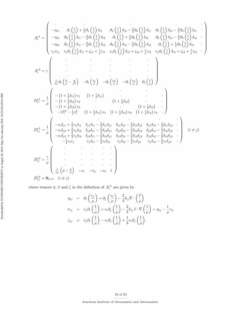
Av1i =

· · · · ·−ηi1 ∂i

(1ρ

)+ 1

3∂1

(1ρ

)δi1 ∂1

(1ρ

)δi2 − 2

3∂2

(1ρ

)δi1 ∂1

(1ρ

)δi3 − 2

3∂3

(1ρ

)δi1 ·

−ηi2 ∂2

(1ρ

)δi1 − 2

3∂1

(1ρ

)δi2 ∂i

(1ρ

)+ 1

3∂2

(1ρ

)δi2 ∂2

(1ρ

)δi3 − 2

3∂3

(1ρ

)δi2 ·

−ηi3 ∂3

(1ρ

)δi1 − 2

3∂1

(1ρ

)δi3 ∂3

(1ρ

)δi2 − 2

3∂2

(1ρ

)δi3 ∂i

(1ρ

)+ 1

3∂3

(1ρ

)δi3 ·

vjπij vj∂j

(1ρ

)δi1 + ζi1 + 1

ρτi1 vj∂j

(1ρ

)δi2 + ζi2 + 1

ρτi2 vj∂j

(1ρ

)δi3 + ζi3 + 1

ρτi3 ·

Av2i = γ

· · · · ·· · · · ·· · · · ·· · · · ·

1a0∂i

(φρ −

pρ2

)−∂i

(v1ρ

)−∂i

(v2ρ

)−∂i

(v3ρ

)∂i

(1ρ

)

Dv1ii =

1

ρ

· · · · ·

−(1 + 1

3δi1)v1

(1 + 1

3δi1)

· · ·−(1 + 1

3δi2)v2 ·

(1 + 1

3δi2)

· ·−(1 + 1

3δi3)v3 · ·

(1 + 1

3δi3)

·−|~v|2 − 1

3v2i

(1 + 1

3δi1)v1

(1 + 1

3δi2)v2

(1 + 1

3δi3)v3 ·

Dv1ij =

1

ρ

· · · · ·

−viδj1 + 23vjδi1 δj1δi1 − 2

3δi1δj1 δj1δi2 − 23δi1δj2 δj1δi3 − 2

3δi1δj3 ·−viδj2 + 2

3vjδi2 δj2δi1 − 23δi2δj1 δj2δi2 − 2

3δi2δj2 δj2δi3 − 23δi2δj3 ·

−viδj3 + 23vjδi3 δj3δi1 − 2

3δi3δj1 δj3δi2 − 23δi3δj2 δj3δi3 − 2

3δi3δj3 ·− 1

3vivj vjδi1 − 23viδj1 vjδi2 − 2

3viδj2 vjδi3 − 23viδj3 ·

(i 6= j)

Dv2ii =

γ

ρ

· · · · ·· · · · ·· · · · ·· · · · ·

1a0

(φ− p

ρ

)−v1 −v2 −v3 1

Dv2ij = 05×5 (i 6= j)

where tensors η, π and ζ in the definition of Av1i are given by

ηij = ∂i

(vjρ

)+ ∂j

(viρ

)− 2

3δij∇ ·

(~v

ρ

)πij = vj∂i

(1

ρ

)+ vi∂j

(1

ρ

)− 2

3δij ~v · ∇

(1

ρ

)= ηij −

1

ρτij

ζij = vj∂i

(1

ρ

)− vi∂j

(1

ρ

)+

1

3vi∂j

(1

ρ

).

23 of 23

American Institute of Aeronautics and Astronautics

Dow

nloa

ded

by S

TA

NFO

RD

UN

IVE

RSI

TY

on

Aug

ust 3

0, 2

014

| http

://ar

c.ai

aa.o

rg |

DO

I: 1

0.25

14/6

.201

4-23

00