Embed Size (px)
Citation preview
Czech Technical University in PragueFaculty of Mechanical Engineering
Ing. Petr Parık
An Out-of-core Sparse Direct Solver
for Very Large Finite Element Problems
Ph.D. Thesis
Prague 2011

c© Petr Parık, 2011
Petr Parık
An Out-of-core Sparse Direct Solver
for Very Large Finite Element Problems
Ph.D. Thesis
Czech Technical University in Prague2011

Contents
1 Introduction 13
2 Overview 172.1 Solution of linear systems . . . . . . . . . . . . . . . . . . . . . . . . . . . 17
2.1.1 Direct methods . . . . . . . . . . . . . . . . . . . . . . . . . . . . . 182.1.2 Iterative methods . . . . . . . . . . . . . . . . . . . . . . . . . . . . 21
2.2 Ordering methods . . . . . . . . . . . . . . . . . . . . . . . . . . . . . . . . 212.2.1 Profile minimization . . . . . . . . . . . . . . . . . . . . . . . . . . 242.2.2 Fill-in minimization . . . . . . . . . . . . . . . . . . . . . . . . . . . 25
2.3 Matrix storage methods . . . . . . . . . . . . . . . . . . . . . . . . . . . . 272.3.1 Dense matrices . . . . . . . . . . . . . . . . . . . . . . . . . . . . . 282.3.2 Sparse matrices . . . . . . . . . . . . . . . . . . . . . . . . . . . . . 29
2.4 Direct solvers . . . . . . . . . . . . . . . . . . . . . . . . . . . . . . . . . . 332.4.1 Standard implementations . . . . . . . . . . . . . . . . . . . . . . . 362.4.2 Available software . . . . . . . . . . . . . . . . . . . . . . . . . . . . 38
3 Aims of the Thesis 39
4 Applied methods 414.1 Matrix storage method . . . . . . . . . . . . . . . . . . . . . . . . . . . . . 41
4.1.1 K3 storage format . . . . . . . . . . . . . . . . . . . . . . . . . . . . 434.2 Ordering method . . . . . . . . . . . . . . . . . . . . . . . . . . . . . . . . 47
4.2.1 Minimum degree algorithm . . . . . . . . . . . . . . . . . . . . . . . 484.3 Solution method . . . . . . . . . . . . . . . . . . . . . . . . . . . . . . . . 54
4.3.1 Symmetric block sparse factorization . . . . . . . . . . . . . . . . . 554.4 PMD implementation concepts . . . . . . . . . . . . . . . . . . . . . . . . 60
4.4.1 Parameter passing . . . . . . . . . . . . . . . . . . . . . . . . . . . 614.4.2 Memory allocation . . . . . . . . . . . . . . . . . . . . . . . . . . . 614.4.3 Input and output files . . . . . . . . . . . . . . . . . . . . . . . . . 63
5 Results and discussion 655.1 Proposed algorithms . . . . . . . . . . . . . . . . . . . . . . . . . . . . . . 65
5.1.1 Matrix storage method . . . . . . . . . . . . . . . . . . . . . . . . . 655.1.2 Ordering method . . . . . . . . . . . . . . . . . . . . . . . . . . . . 71
5
CONTENTS
5.1.3 Solution method . . . . . . . . . . . . . . . . . . . . . . . . . . . . 805.2 Solver implementation . . . . . . . . . . . . . . . . . . . . . . . . . . . . . 82
5.2.1 Ordering phase . . . . . . . . . . . . . . . . . . . . . . . . . . . . . 835.2.2 Assembly phase . . . . . . . . . . . . . . . . . . . . . . . . . . . . . 835.2.3 Factorization phase . . . . . . . . . . . . . . . . . . . . . . . . . . . 845.2.4 Solution phase . . . . . . . . . . . . . . . . . . . . . . . . . . . . . . 84
5.3 FEM applications . . . . . . . . . . . . . . . . . . . . . . . . . . . . . . . . 855.3.1 Example problems . . . . . . . . . . . . . . . . . . . . . . . . . . . 865.3.2 Engineering problems . . . . . . . . . . . . . . . . . . . . . . . . . . 88
6 Conclusions 93
Bibliography 97
Appendix 101
A Selected FEM problems 101A.1 Example problems . . . . . . . . . . . . . . . . . . . . . . . . . . . . . . . 101
A.1.1 Elastostatics . . . . . . . . . . . . . . . . . . . . . . . . . . . . . . . 101A.1.2 Dynamics . . . . . . . . . . . . . . . . . . . . . . . . . . . . . . . . 101A.1.3 Plasticity . . . . . . . . . . . . . . . . . . . . . . . . . . . . . . . . 102A.1.4 Creep . . . . . . . . . . . . . . . . . . . . . . . . . . . . . . . . . . 102A.1.5 Geomerically nonlinear problems . . . . . . . . . . . . . . . . . . . 102A.1.6 Contact . . . . . . . . . . . . . . . . . . . . . . . . . . . . . . . . . 103
A.2 Engineering problems . . . . . . . . . . . . . . . . . . . . . . . . . . . . . . 103A.2.1 10 . . . . . . . . . . . . . . . . . . . . . . . . . . . . . . . . . . . . 104A.2.2 A98ABT001 1 . . . . . . . . . . . . . . . . . . . . . . . . . . . . . . 105A.2.3 ADS . . . . . . . . . . . . . . . . . . . . . . . . . . . . . . . . . . . 106A.2.4 BUBEN . . . . . . . . . . . . . . . . . . . . . . . . . . . . . . . . . 107A.2.5 C2 . . . . . . . . . . . . . . . . . . . . . . . . . . . . . . . . . . . . 108A.2.6 C3 . . . . . . . . . . . . . . . . . . . . . . . . . . . . . . . . . . . . 109A.2.7 C5 . . . . . . . . . . . . . . . . . . . . . . . . . . . . . . . . . . . . 110A.2.8 COUV9 . . . . . . . . . . . . . . . . . . . . . . . . . . . . . . . . . 111A.2.9 DOCHL . . . . . . . . . . . . . . . . . . . . . . . . . . . . . . . . . 112A.2.10 K1 . . . . . . . . . . . . . . . . . . . . . . . . . . . . . . . . . . . . 113A.2.11 K3 . . . . . . . . . . . . . . . . . . . . . . . . . . . . . . . . . . . . 114A.2.12 P6 LIN, P6 QUAD . . . . . . . . . . . . . . . . . . . . . . . . . . . 115A.2.13 SH . . . . . . . . . . . . . . . . . . . . . . . . . . . . . . . . . . . . 116A.2.14 SHVO . . . . . . . . . . . . . . . . . . . . . . . . . . . . . . . . . . 117
B Solver file formats 119B.1 Formatted files . . . . . . . . . . . . . . . . . . . . . . . . . . . . . . . . . 119
B.1.1 name.I4 (FEFS, FESD) . . . . . . . . . . . . . . . . . . . . . . . . 119B.2 Unformatted files . . . . . . . . . . . . . . . . . . . . . . . . . . . . . . . . 121
6
CONTENTS
B.2.1 IDEQC . . . . . . . . . . . . . . . . . . . . . . . . . . . . . . . . . . 121B.2.2 IDEQI . . . . . . . . . . . . . . . . . . . . . . . . . . . . . . . . . . 121B.2.3 IDEQR . . . . . . . . . . . . . . . . . . . . . . . . . . . . . . . . . . 122
C Solver source code 123C.1 Program FESD . . . . . . . . . . . . . . . . . . . . . . . . . . . . . . . . . 123C.2 Program FESDA . . . . . . . . . . . . . . . . . . . . . . . . . . . . . . . . 131
7
Acknowledgements
The work presented in this thesis was carried out at the Department of Impact and Wavesin Solids of the Institute of Thermomechanics, Academy of Sciences of the Czech republic.
I would like to express the deep gratitude and thanks to my supervisor Dr. Jirı Plesekfor his patience with my work and for all the motivation and guidance endowed upon me.I would also like to thank all members of the department for their willingness to discussand comment my work at any time, and for their kind and friendly attitude. Last but notleast, I would like to thank my parents Hana and Miroslav for their unconditional loveand support which enabled me to pursue the highest goals in life.
8
Abstract
An out-of-core sparse direct solver for very large finite
element problems
This thesis is focused on enhancing numerical methods used in the direct solution of largelinear equation systems that arise in practical application of the finite element method(FEM) in solid continuum mechanics. A linear equation system forms the basis of everyFEM problem, therefore, its fast and efficient solution is always desirable. Large problemsare defined as problems for which the requirements on memory storage and computationaltime make the solution difficult using available computers. Very large problems cannot besolved unless the solution is performed partially out of core, using a disk storage, whichunfortunately reduces efficiency.
The first part of this thesis presents a critical overview of fundamental methods usedfor the solution of linear systems of equations, such as storage methods for coefficientmatrices, ordering methods, and solution methods, and also discusses common directsolver implementations. Next part describes in detail the selected K3 sparse matrix stor-age format, the approximate minimum degree ordering (AMD), and the symmetric LUfactorization. In the final part, the enhancements to the aforementioned numerical al-gorithms are proposed with regard to the out-of-core solution of large sparse symmetricpositive-definite linear systems. In particular, an efficient block sparse storage format forthe coefficient matrix based on the K3 format is proposed, together with a modified min-imum degree algorithm that includes symbolic assembly and works on the block nonzerostructure of the matrix, also including a modified left-looking factorization algorithm thathas low storage requirements suitable for out-of-core solution.
The proposed numerical algorithms are assessed by means of an out-of-core sparsedirect solver implemented into the PMD system, an in-house software package for FEManalysis. Results are presented for both test problems and several large real-world en-gineering problems. Furthermore, a performance comparison with the existing PMD’slinear solver, based on the frontal solution method, is presented, which demonstrates thevalidity and efficiency of the proposed algorithms.
9
Notation and symbols
A coefficient matrix
A permuted coefficient matrixAij submatrix of the coefficient matrixAk partially reduced coefficient matrixA set of variables adjacent to a variable in the quotient graphaij entry of the coefficient matrix
a(k)ij entry of the partially reduced coefficient matrix
b right-hand side vectorD diagonal matrix factorDii submatrix of the matrix factord order of block submatrixd number of nodal degrees of freedomd external degree
d approximate degree
d approximate degreed approximate degreedii entry of the matrix factorE set of graph edgesE set of edges between variables in the quotient graphE set of edges between variables and elements in the quotient graphE set of elements adjacent to a variable in the quotient graphG graphG elimination graphG quotient graphk actual elimination stepL unit lower triangular matrix factor
L lower triangular Cholesky matrix factorLji submatrix of the matrix factorL set of variables adjacent to an element in the quotient graphL length of matrix storageLnz length of all nonzero submatrices in the coefficient matrixlji entry of the matrix factorM number of matrix block rowsm number of matrix rows
10
NOTATION AND SYMBOLS
N number of mesh nodesN number of matrix block columnsn number of matrix columnsn order of square matrixNnz number of nonzero blocks in matrixnnz number of nonzero entries in matrixP left permutation matrixp actual pivotQ right permutation matrixQ orthogonal matrix factorR upper triangular matrix factorS set of variables in supervariable in the quotient grapht true degreeU upper triangular matrix factorV set of graph verticesV set of variables in the quotient graphV set of elements in the quotient graphx solution vectory reduced right-hand side vectorz permuted solution vector
BUF(LBUF) buffer for equations (coefficient matrix)ICL integer-to-real size factorIDCOM file name.CMN, common problem dataIDDM1 file name.DM1, auxiliary data (frontal solver)IDELM file name.ELM, element stiffness matricesIDEQ1 file name.EQ1, factorized equations (frontal solver)IDEQC file name.EQC, auxiliary data (sparse direct solver)IDEQI file name.EQI, matrix block indices (sparse direct solver)IDEQR file name.EQR, factorized equations (sparse direct solver)IDP file name.P, mesh dataIDRHS file name.RHS, right-hand side vectorsIDSOL file name.SOL, solution vectorsIFIXV(NFIXV) indices of fixed variables (constrained degrees of freedom)INET(LINET) indices of nodes in elementsINT integer workspaceIPNOD(NNOD) permutation vector applied to nodesIPSOL(LSOL) permutation vector applied to degrees of freedomKFES sparse direct solver statusLBUF1 actual size of array BUF in assembly (≤ SBUF1)LBUF2 actual size of array BUF in factorization (≤ SBUF2)LI size of the workspace
11
NOTATION AND SYMBOLS
LINET length of array INET
LNNDF length of array NNDF
LNNET length of array NNET
LSMTX maximum length of nodal submatrix (block)LSOL length of the solution vector (including reaction forces)name problem data nameMBD(NNOD) number of variables per blockMBP(NBLK2) pointers to blocks (nodal submatrices)MCI(NBLK2) nodal column indices for matrix blocksMRP(NPIV+1) nodal row pointers for matrix blocksNASV number of load cases (right-hand sides)NBLK1 number of nonzero blocks in assembled matrixNBLK2 number of nonzero blocks in factorized matrixNELEM number of mesh elementsNFIXV number of fixed variablesNNDF(LNNDF) number of degrees of freedom per nodeNNET(LNNET) number of nodes per elementNNOD number of mesh nodesNPIV number of pivot blocks (NNOD minus number of constrained nodes)NVAR number of variables (LSOL minus number of reaction forces)R real number workspaceRHS(LSOL,NASV) right-hand side vectorsSBUF1 summed length of blocks in assembled matrixSBUF2 summed length of blocks in factorized matrix
÷ integer division operator, used to distinguish integer division (thatinvolves a remainder) from real-number division (operator /)
12
Chapter 1
Introduction
The finite element method [5] is without doubt one of the most important numerical tech-niques available in solid continuum mechanics. By definition, it is a variational method forthe approximate solution of boundary value problems, where partial differential equationsare transformed into a corresponding ordinary differential system, or in the case of steadystate problems, into a corresponding algebraic system. The finite element method wasimplemented on computers uncountable times since its early years in 1950s. Today, manysoftware packages, both commercial and free, are available that provide the capabilitiesfor a comprehensive finite element analysis in many areas of solid and fluid continuummechanics, beginning with the creation of the finite element mesh (usually automatized)and ending with the evaluation of the numerical results aided by their visual representa-tion, using various contour plots. Robustness, ease of use, and readily available softwaresignificantly contributed to the popularity of the finite element method in engineeringpractice in past decades.
An important advantage of the finite element method is that it is not limited to simpledomains or to uniform regions. Meshes can be of any shape, and different elements canhave different sizes and shapes. Therefore, quite complicated domains, such as wholemachines, can be approximated very closely, provided that the mesh is sufficiently fine.The accuracy of the numerical solution obtained by the finite element method can beeasily affected by refining or coarsening the size and shape of the elements and, therefore,theoretically arbitrary precision can be achieved in any part of the mesh. In reality, refin-ing of the finite element mesh is severely limited, since finer meshes require substantiallymore storage space and computational time in order to be processed. Therefore, finiteelement meshes are usually constructed to be finer in the parts of interest, and coarser inthe other parts. Unfortunately, parts of the mesh that have complex shapes also need tobe refined so that they appropriately represent the geometry, thus, the ultimate numberof equations that describe the problem can be often relatively high.
Some fifty years ago, the size of the largest problem computable by the finite elementmethod using a state-of-the-art computer was only one or two hundred equations, andthe problems were limited to very simple geometries and a few mesh elements. Today,computers are incomparably more powerful and have much larger capacity in storagespace, which allows the finite element problems to have about 105 to 107 equations. Of
13
CHAPTER 1. INTRODUCTION
course, these sizes are relevant to steady state problems that lead to a system of linearequations.
In the past decades, much attention has been directed towards an efficient implemen-tation of solvers for large finite element problems. Direct methods, based on the Gaussianelimination, could not be overly used due to the limited capacity of available computers,which favored iterative methods that had lower computational demands but were muchless robust. With the increasing performance of computers in late 1980s it became pos-sible to implement skyline direct solvers, which exploited the fact that the skyline of thecoefficient matrix was retained during the factorization. Today, skyline solvers are stillmistakenly considered by some as the ultimate direct solvers for large finite element prob-lems. However, the research conducted in the last decade showed that very large finiteelement problems could be solved more efficiently by a general sparse direct solver thatwould work only with nonzero entries of the coefficient matrix.
The work presented in this thesis has been motivated by the need for a new directlinear solver in the PMD finite element system (see Section 2.4.2 and Section 4.4) to allowefficient computations on large finite element problems. The PMD’s existing linear solverhas been developed in late 1970s and is based on the frontal solution method [24] that ismemory-efficient and robust. However, this method is generally unsuitable for large finiteelement problems, since the demands on the disk (out-of-core) storage and the solutiontime are impractical in most cases. State-of-the-art preordering techniques that reducestorage requirements and computational costs cannot be applied to the frontal solutionmethod, and therefore a completely new solver code has to be developed. The performanceof the existing frontal solver is also a limiting factor in the application of some more robustsolution methods for nonlinear and dynamic problems, where the need for solving a largelinear equation system occurs repetitively and thus an efficient implementation is crucial.
The basic methods involved in a sparse direct solution are the matrix storage method,the (pre)ordering method, and the solution (factorization) method, which are all interde-pendent to some degree. The storage of the whole coefficient matrix (or approximately onehalf in symmetric cases) is obviously never acceptable except the smallest problems thatare however not practical. Matrix storage schemes thus try to exploit sparsity, symmetryand other properties of the coefficient matrix to store as few zero entries of the matrixas possible. Although it is perfectly reasonable not to store any nonzero entries, whichis clearly the most efficient option and is indeed used for example in iterative methods,direct methods unfortunately spoil the sparsity structure by introducing new nonzero en-tries during the triangularization (factorization) of the coefficient matrix. This occurenceof new nonzeros is called the fill-in and presents a major drawback and difficulty of directmethods. The initial nonzero structure of the matrix as well as the final nonzero structure(the amount of fill-in) can be substantially affected by using an ordering method. Storageof the coefficient matrix in the case of large problems requires a careful consideration,since it has a significant impact on the practical implementation of the solution method.
Ordering methods switch rows and columns of the matrix to obtain another, preferablymore suitable, order of pivots on the main diagonal. An important consequence is that theresulting nonzero structure of the reordered matrix may allow an efficient storage and/or
14
factorization using direct methods. Different ordering methods usually imply certain typesof matrix storage schemes. For example, profile minimization algorithms move all nonzeroentries close to the main diagonal, yielding a band or skyline matrix, therefore, a band orskyline storage format is ideal. The fill-in can occur only within the band or under theskyline of the coefficient matrix, thus it is also effectively reduced. Fill-in minimizationalgorithms are used specifically to reduce the fill-in, but they result in a more complicatednonzero structure requiring more complex storage schemes. Ordering methods usuallywork with graphs representing the nonzero structure of the matrix, and since operationson graphs are computationally expensive, the time complexity rises quickly in the case oflarge problems. However, without a suitable ordering, the direct solution of large problemsis generally impossible due to uncontrollable fill-in.
The sparse direct solution is mostly performed using a variant of the Gaussian elimina-tion. In order to be efficient, the method must exploit the sparsity of the coefficient matrixby avoiding unnecessary operations on zero entries. This largely depends on the employedmatrix storage scheme and also on the used ordering method. Small and medium prob-lems can be usually fully solved in memory (in core), but in the case of large problems,it may be necessary to store a part of the matrix data temporarily on the disk (out ofcore). Out-of-core solution of course involves much more complicated algorithms andsince the disk storage is much slower than the memory storage, great care must be takento implement the solution method efficiently.
The thesis is organized in the following way. Overview of the numerical methodsused in linear equation solvers is presented in Chapter 2. Based on the state of the artsummarized in the overview, the particular aims of the thesis are formulated in Chapter 3.Chapter 4 explains in detail the methods mentioned in the overview which have beenselected as the basis for the sparse direct solver implementation. Chapter 5 describes anddiscusses the proposed modifications to the applied methods and algorithms, deals withthe sparse direct solver implementation, and presents applications in the finite elementanalysis, including a comparison with the frontal solver. Finally, some conclusions aredrawn in Chapter 6, summarizing results and pointing to further research.
Publications
Papers listed below were published during the course of the work and were compiled intothe thesis.
• Parık P. and Plesek J. (2009). Assessments of the implementation of the minimumdegree ordering algorithms. Pollack Periodica, International Journal for Engineer-ing and Information Sciences, 4, 3, pp. 121–128.
• Parık P. (2009). Performance tests of the minimum degree ordering algorithm.Engineering Mechanics 2009, pp. 929–935.
15
CHAPTER 1. INTRODUCTION
• Parık P. (2008). Sparse storage schemes. In: Okrouhlık M., editor. Numericalmethods in computational mechanics, pp. 272–281. Institute of ThermomechanicsASCR, Prague.
• Parık P. (2008). Implementation of a sparse direct solver for large linear systems.Vypocty konstrukcı metodou konecnych prvku 2008, pp. 98–101.
• Parık P. (2007). Sparse direct solver with fill-in optimization. Engineering Mechan-ics 2007.
• Parık P. (2005). Numericka implementace linearnıho resice na bazi algoritmu AMD.Summer Workshop of Applied Mechanics 2005, pp. 75–84.
16
Chapter 2
Overview
In this chapter, the state of the art in the numerical techniques for solving linear equationsystems is presented, with a special interest in the direct solution of large systems withsparse symmetric positive definite coefficient matrices, that are the most common in thefinite element analysis of solids and structures. The first section summarizes the methodsavailable for solving linear equation systems. The second section deals with the orderingmethods and their importance in the direct solution of large systems. The third sectiondescribes the storage methods for dense and sparse matrices. Finally, the last sectiondiscusses direct solvers and their common implementations.
2.1 Solution of linear systems
A set of simultaneous linear equations (linear equation system) can be written conve-niently in the matrix form
Ax = b, (2.1)
where A is the coefficient matrix, x is the solution vector and b is the right-hand sidevector. The straightforward solution readily obtained from equation (2.1) is
x = A−1b, (2.2)
where A−1 is the inverse of matrix A. However, computing the inverse is almost neveran appropriate nor computationally feasible way for solving system (2.1).
A linear equation system with a handful of unknowns may of course be solved byvirtually any method, but as the order of the system (number of equations) increases, thechoice of proper numerical techniques quickly becomes crucial. If chosen unwisely, thetime and/or storage space required to obtain the solution may be either too large, or thesolution may not be possible at all.
Numerical methods for solving the linear equation system (2.1) are divided into twodistinct classes, direct methods and iterative methods.
In direct methods, an exact solution is obtained after a finite number of operations.The accuracy of a direct solution is however affected by the employed finite-precisionarithmetic.
17
CHAPTER 2. OVERVIEW
Year Order
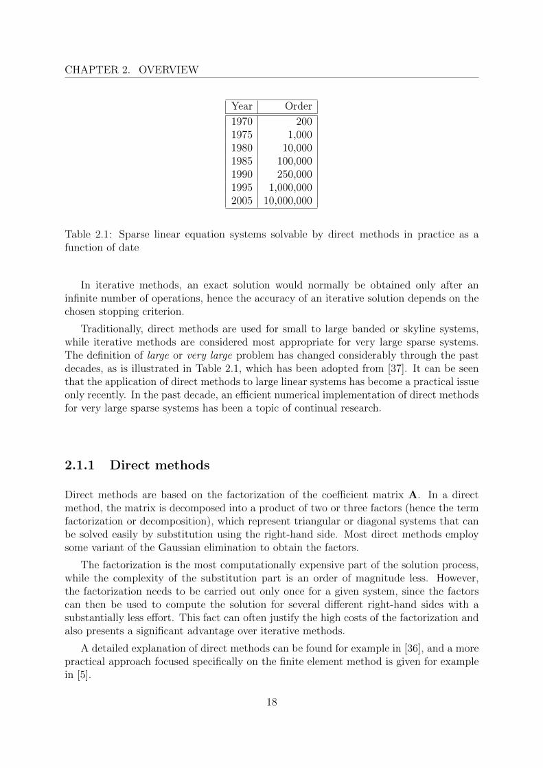
1970 2001975 1,0001980 10,0001985 100,0001990 250,0001995 1,000,0002005 10,000,000
Table 2.1: Sparse linear equation systems solvable by direct methods in practice as afunction of date
In iterative methods, an exact solution would normally be obtained only after aninfinite number of operations, hence the accuracy of an iterative solution depends on thechosen stopping criterion.
Traditionally, direct methods are used for small to large banded or skyline systems,while iterative methods are considered most appropriate for very large sparse systems.The definition of large or very large problem has changed considerably through the pastdecades, as is illustrated in Table 2.1, which has been adopted from [37]. It can be seenthat the application of direct methods to large linear systems has become a practical issueonly recently. In the past decade, an efficient numerical implementation of direct methodsfor very large sparse systems has been a topic of continual research.
2.1.1 Direct methods
Direct methods are based on the factorization of the coefficient matrix A. In a directmethod, the matrix is decomposed into a product of two or three factors (hence the termfactorization or decomposition), which represent triangular or diagonal systems that canbe solved easily by substitution using the right-hand side. Most direct methods employsome variant of the Gaussian elimination to obtain the factors.
The factorization is the most computationally expensive part of the solution process,while the complexity of the substitution part is an order of magnitude less. However,the factorization needs to be carried out only once for a given system, since the factorscan then be used to compute the solution for several different right-hand sides with asubstantially less effort. This fact can often justify the high costs of the factorization andalso presents a significant advantage over iterative methods.
A detailed explanation of direct methods can be found for example in [36], and a morepractical approach focused specifically on the finite element method is given for examplein [5].
18
2.1. SOLUTION OF LINEAR SYSTEMS
LU factorization
An LU factorization of a square matrix A takes the form
A = LU, (2.3)
where L is a lower triangular matrix and U is an upper triangular matrix. The factors arenot defined uniquely by equation (2.3) unless further constraints are imposed. To obtaina unique LU factorization, L is usually limited to a unit lower triangular matrix.
Substituting equation (2.3) into equation (2.1) yields
LUx = b. (2.4)
Using another substitutionUx = y, (2.5)
the solution of system (2.4) can be divided into two parts.The first part of the solution, called forward substitution, is
Ly = b, (2.6)
from which the reduced right-hand side vector y is obtained.The second part of the solution, called back substitution, is
Ux = y, (2.7)
from which the solution vector x and the solution of systems (2.4) and (2.1) is obtained.The solution of system (2.1) using the LU factorization is easy to carry out since
systems (2.6) and (2.7) are triangular. Other direct methods employ a similar procedurefor computing the solution using the factors.
Cholesky factorization
Let A be a symmetric matrix. Then
AT= A. (2.8)
Let A be a positive definite matrix. Then it is symmetric and
uTAu > 0 (2.9)
for any real nonzero vector u.A Cholesky factorization of a symmetric positive definite matrix A takes the form
A = LLT, (2.10)
where L is a lower triangular matrix. The advantage of this method is that, unlike theother methods, it is always numerically stable, therefore no pivoting is necessary. Choleskyfactorization is about twice as efficient as the LU factorization in both the computationalcosts and the storage requirements. Aside from solving system (2.1) it is also often usedto check for the positive definiteness of a matrix.
19

CHAPTER 2. OVERVIEW
LDLT factorization
An LDLT factorization of a symmetric matrix A takes the form
A = LDLT, (2.11)
where L is an unit lower triangular matrix and D is a diagonal matrix. The solutionis computed in the same way as in the LU factorization, substituting U ≡ DLT. Thismethod is of particular interest in numerical analysis since it is comparable to the Choleskyfactorization in efficiency, but is applicable to both positive definite and indefinite matri-ces.
QR factorization
Let Q be an orthogonal matrix. Then
QT = Q−1. (2.12)
A QR factorization of a matrix A takes the form
A = QR, (2.13)
where Q is an orthogonal matrix and R is an upper triangular matrix. The factors arecomputed using orthogonalization algorithms such as the Gram-Schmidt process, House-holder transformations or Givens rotations. QR factorization can be used to solve sys-tem (2.1), but its computational costs are high over the LU factorization. However, itis valuable for solving overdetermined systems, i.e., when the coefficient matrix A inequation (2.1) is rectangular, which is a common case in the least squares problems.
Numerical stability and pivoting
Unless the matrix is symmetric and positive definite, the factorization can run into diffi-culties when any diagonal entry (pivot) is zero or very small relative to other row entries.To prevent a numerical breakdown of the factorization, partial or full pivoting must beapplied to the matrix.
In partial pivoting, the entry with the largest absolute value in the pivot column ischosen as the next pivot, switching the correspoding rows. Unlike full pivoting, partialpivoting does not change the order of unknowns.
In full pivoting, the entry with the largest absolute value in the remaining uneliminatedrows is chosen as the next pivot, switching the correspoding rows and columns.
Partial pivoting is sufficient to ensure the numerical stability of the factorization inmost cases. Generally, it is ill-advised to perform the factorization on indefinite matriceswithout some form of pivoting.
20
2.2. ORDERING METHODS
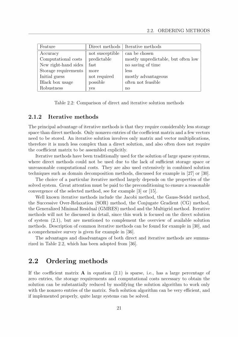
Feature Direct methods Iterative methods
Accuracy not susceptible can be chosenComputational costs predictable mostly unpredictable, but often lowNew right-hand sides fast no saving of timeStorage requirements more lessInitial guess not required mostly advantageousBlack box usage possible often not feasibleRobustness yes no
Table 2.2: Comparison of direct and iterative solution methods
2.1.2 Iterative methods
The principal advantage of iterative methods is that they require considerably less storagespace than direct methods. Only nonzero entries of the coefficient matrix and a few vectorsneed to be stored. An iterative solution involves only matrix and vector multiplications,therefore it is much less complex than a direct solution, and also often does not requirethe coefficient matrix to be assembled explicitly.
Iterative methods have been traditionally used for the solution of large sparse systems,where direct methods could not be used due to the lack of sufficient storage space orunreasonable computational costs. They are also used extensively in combined solutiontechniques such as domain decomposition methods, discussed for example in [27] or [30].
The choice of a particular iterative method largely depends on the properties of thesolved system. Great attention must be paid to the preconditioning to ensure a reasonableconvergence of the selected method, see for example [3] or [15].
Well known iterative methods include the Jacobi method, the Gauss-Seidel method,the Successive Over-Relaxation (SOR) method, the Conjugate Gradient (CG) method,the Generalized Minimal Residual (GMRES) method and the Multigrid method. Iterativemethods will not be discussed in detail, since this work is focused on the direct solutionof system (2.1), but are mentioned to complement the overview of available solutionmethods. Description of common iterative methods can be found for example in [30], anda comprehensive survey is given for example in [36].
The advantages and disadvantages of both direct and iterative methods are summa-rized in Table 2.2, which has been adopted from [36].
2.2 Ordering methods
If the coefficient matrix A in equation (2.1) is sparse, i.e., has a large percentage ofzero entries, the storage requirements and computational costs necessary to obtain thesolution can be substantially reduced by modifying the solution algorithm to work onlywith the nonzero entries of the matrix. Such solution algorithm can be very efficient, andif implemented properly, quite large systems can be solved.
21
CHAPTER 2. OVERVIEW
As already mentioned in Subsection 2.1.1, direct methods generally require pivotingto ensure the numerical stability of the factorization. In the sparse case, pivoting (calledordering) is also necessary to preserve the sparsity in the factors. Unfortunately, pivotingfor numerical stability and pivoting for sparsity preservation are contradictory goals, andhave been a topic of research.
For example, the factorization of an arrowhead matrix
A =
∗ ∗ ∗ · · · ∗∗ ∗∗ ∗...
. . .
∗ ∗
(2.14)
leads to dense triangular factors. By switching the first pivot with the last pivot, theobtained matrix
B =
∗ ∗. . .
...∗ ∗∗ ∗
∗ · · · ∗ ∗ ∗
(2.15)
exhibits no fill-in, i.e., there will not be any nonzero in the entries that were zero in theoriginal matrix. Since the switching of rows and columns are elementary matrix operationsthat do not change the solution of the associated linear system, matrices (2.14) and (2.15)are equivalent.
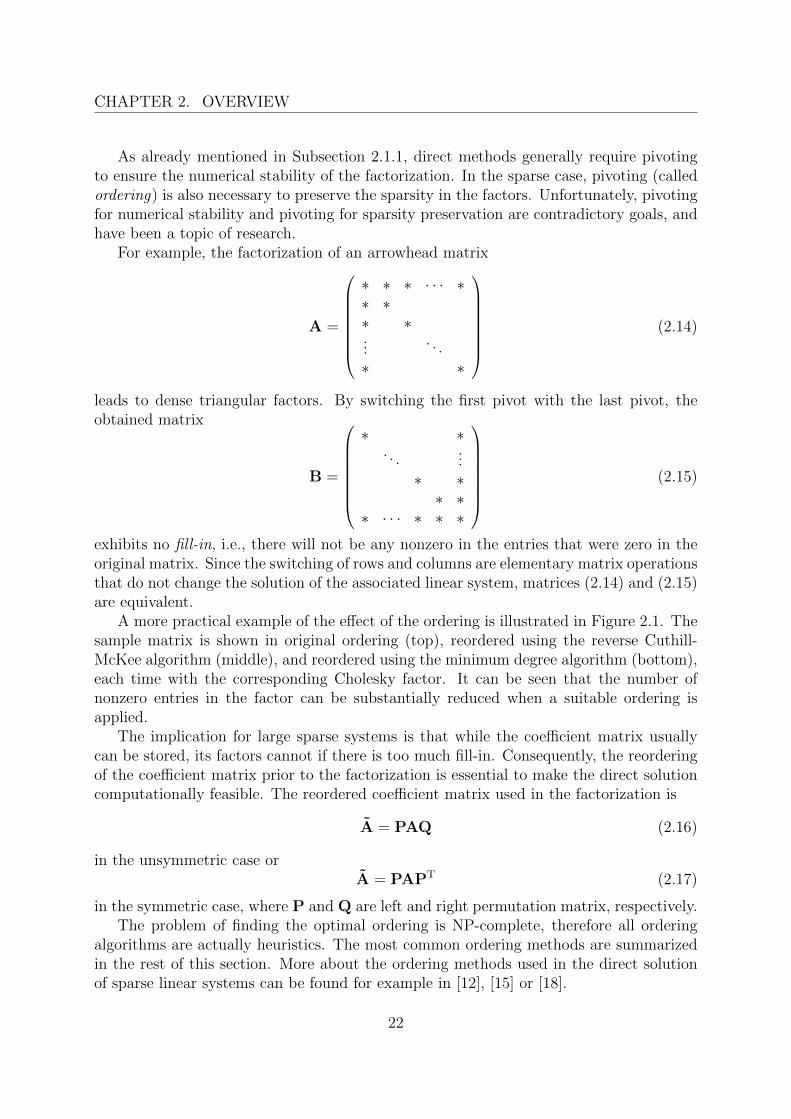
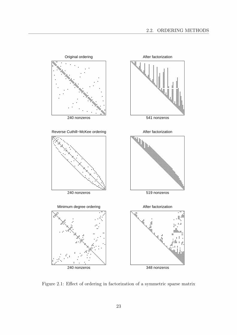
A more practical example of the effect of the ordering is illustrated in Figure 2.1. Thesample matrix is shown in original ordering (top), reordered using the reverse Cuthill-McKee algorithm (middle), and reordered using the minimum degree algorithm (bottom),each time with the corresponding Cholesky factor. It can be seen that the number ofnonzero entries in the factor can be substantially reduced when a suitable ordering isapplied.
The implication for large sparse systems is that while the coefficient matrix usuallycan be stored, its factors cannot if there is too much fill-in. Consequently, the reorderingof the coefficient matrix prior to the factorization is essential to make the direct solutioncomputationally feasible. The reordered coefficient matrix used in the factorization is
A = PAQ (2.16)
in the unsymmetric case orA = PAPT (2.17)
in the symmetric case, where P and Q are left and right permutation matrix, respectively.The problem of finding the optimal ordering is NP-complete, therefore all ordering
algorithms are actually heuristics. The most common ordering methods are summarizedin the rest of this section. More about the ordering methods used in the direct solutionof sparse linear systems can be found for example in [12], [15] or [18].
22
2.2. ORDERING METHODS
240 nonzeros
Original ordering
240 nonzeros
Reverse Cuthill−McKee ordering
240 nonzeros
Minimum degree ordering
541 nonzeros
After factorization
519 nonzeros
After factorization
348 nonzeros
After factorization
Figure 2.1: Effect of ordering in factorization of a symmetric sparse matrix
23
CHAPTER 2. OVERVIEW
1 ∗ ∗2 ∗ ∗ ∗
3 ∗ ∗ ∗∗ 4 ∗ ∗∗ ∗ 5 ∗ ∗
∗ ∗ ∗ 6∗ ∗ ∗ 7 ∗ ∗ ∗∗ ∗ 8 ∗ ∗
∗ ∗ ∗ ∗ 9 ∗∗ ∗ ∗ 10
10 8 4 1
9 7 3 6
5
2
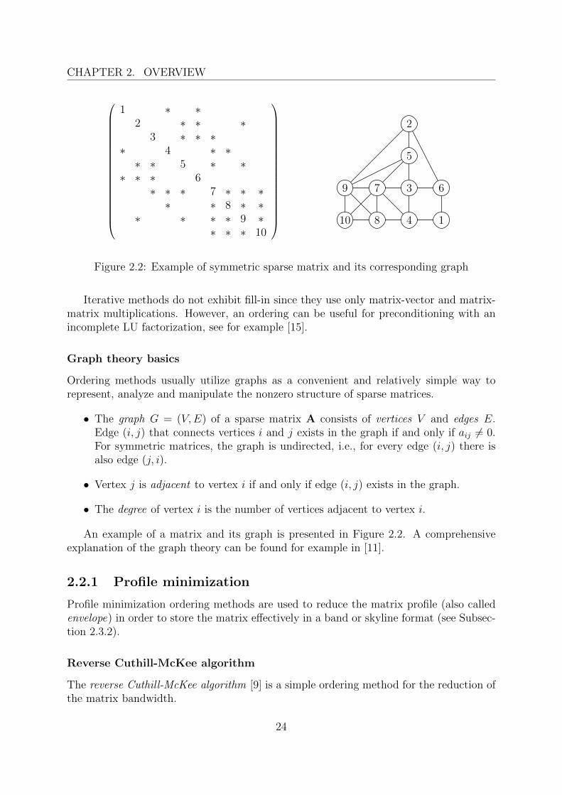
Figure 2.2: Example of symmetric sparse matrix and its corresponding graph
Iterative methods do not exhibit fill-in since they use only matrix-vector and matrix-matrix multiplications. However, an ordering can be useful for preconditioning with anincomplete LU factorization, see for example [15].
Graph theory basics
Ordering methods usually utilize graphs as a convenient and relatively simple way torepresent, analyze and manipulate the nonzero structure of sparse matrices.
• The graph G = (V,E) of a sparse matrix A consists of vertices V and edges E.Edge (i, j) that connects vertices i and j exists in the graph if and only if aij 6= 0.For symmetric matrices, the graph is undirected, i.e., for every edge (i, j) there isalso edge (j, i).
• Vertex j is adjacent to vertex i if and only if edge (i, j) exists in the graph.
• The degree of vertex i is the number of vertices adjacent to vertex i.
An example of a matrix and its graph is presented in Figure 2.2. A comprehensiveexplanation of the graph theory can be found for example in [11].
2.2.1 Profile minimization
Profile minimization ordering methods are used to reduce the matrix profile (also calledenvelope) in order to store the matrix effectively in a band or skyline format (see Subsec-tion 2.3.2).
Reverse Cuthill-McKee algorithm
The reverse Cuthill-McKee algorithm [9] is a simple ordering method for the reduction ofthe matrix bandwidth.
24
2.2. ORDERING METHODS
The algorithm works as follows:
1. Create a graph according to the nonzero structure of the matrix, and an empty list.
2. Choose a starting vertex, number it 1, and add it to the list.
3. Remove the first vertex from the list, number all unnumbered vertices adjacent tothe vertex in order of their degree, and append them to the end of the list.
4. Unless all vertices are numbered, repeat from step 3.
5. The permutation vector is given by the sequence in which the vertices were num-bered.
Choosing a good starting vertex is the most important part of the algorithm, sincethe obtained ordering is highly dependent on its choice. Several strategies for finding the(pseudo-) peripheral vertices, which are good candidates for the starting vertex, are usedfor this purpose.
The described algorithm is actually the original Cuthill-McKee algorithm, but nor-mally the reverse sequence of vertices is used, since it results in even lower bandwidth(hence the reverse Cuthill-McKee algorithm).
Spectral algorithm
The spectral algorithm for envelope reduction [4] is an ordering method for minimizingthe matrix profile.
The algorithm works as follows:
1. Form a Laplacian matrix according to the nonzero structure of the matrix.
2. Compute the second eigenvector of the Laplacian matrix.
3. Sort the components of the eigenvector in nondecreasing order, and reorder the ma-trix using the corresponding permutation vector Also sort the components in non-increasing order, and compute the corresponding reordering of the matrix. Choosethe permutation that leads to smaller profile.
The most computationally difficult part of the algorithm is the computation of thesecond eigenvector, which is carried out using multilevel approach based on the Lanczosmethod [3]. Numerical results show that the spectral algorithm usually yields betterordering and is faster than the reverse Cuthill-McKee algorithm.
2.2.2 Fill-in minimization
Fill-in minimization ordering methods are used to reduce the fill-in introduced in thefactorization, and are especially useful in the direct solution of large sparse systems.To store the reordered matrix efficiently, a general sparse scheme has to be used (seeSubsection 2.3.2) since the matrix profile may be rather large and the nonzero structureof the matrix usually does not follow any exploitable pattern.
25
CHAPTER 2. OVERVIEW
Minimum degree algorithm
The minimum degree algorithm [34] is one of the most widely used ordering methods sinceit produces factors with relatively low fill-in on a wide range of matrices.
The algorithm works as follows:
1. Create a graph according to the nonzero structure of the matrix.
2. Remove the vertex with minimum degree from the graph. Add edges to the graphso that all vertices adjacent to the removed vertex form a clique (i.e., are all inter-connected with each other).
3. Unless the graph is empty, repeat from step 2.
4. The permutation vector is given by the sequence in which the vertices were removedfrom the graph.
The most computationally difficult part of the algorithm is the computation of vertexdegrees. Since the introduction of the basic algorithm stated above, numerous refinementshas been devised to improve its efficiency.
The state of the art implementation is the approximate minimum degree algorithm byAmestoy, Davis and Duff [1, 2].
Nested dissection algorithm
The nested dissection algorithm [21, 26] is a recursive ordering method based on graphpartitioning. It is known to be theoretically superior to the minimum degree algorithm forsparse symmetric definite matrices, but only very recently the implementations have beenshown that are more efficient than the implementations of the minimum degree algorithm.
The algorithm works as follows:
1. Create a graph according to the nonzero structure of the matrix.
2. Partition the graph into two subgraphs of roughly same size using a small vertexseparator.
3. Repeat step 2 recursively for every subgraph, until the subgraphs are fairly small.
4. The permutation vector is given by the reverse sequence of the vertex separators.The vertices in the top level separator are ordered last, the vertices in the second-to-top level separator are ordered before them, etc.
Finding a good vertex separator is the most important part of the algorithm.Coordinate-based and coordinate-free methods are used for this purpose.
The state of the art implementation is the METIS software package by Karypis andKumar [25].
26
2.3. MATRIX STORAGE METHODS
2.3 Matrix storage methods
In the actual numerical implementation, matrix entries have to be stored in the computermemory in some efficient way. The choice of a storage scheme (also called storage formator storage mode) for a particular problem depends on various factors including the struc-ture of the matrix and the solution method employed. Obviously, all storage schemesdesigned for symmetric matrices can be used for triangular matrices as well.
Direct methods operate primarily on dense matrices, but implementations with sparsematrices became quite popular in recent decades. If the coefficient matrix is stored in ageneral sparse scheme, the occurence of fill-in must be carefully taken into consideration.
Iterative methods operate primarily on sparse matrices and since they do not modifymatrix entries, the implementation of any storage scheme is relatively straightforward. Aparticular storage scheme can be chosen purely based on the properties of the coefficientmatrix (symmetry, profile, block structure, etc.).
The most common matrix storage schemes are summarized in this section. For a moredetailed survey, see [36], [3] and [30].
Fill-in consideration
In dense, band and skyline matrix storage schemes (to be explained), the fill-in does notconstitute a problem, since all storage locations for matrix entries where the fill-in mightoccur are present implicitly. In general sparse storage schemes, such as the compressedrow format (and other similar schemes), storage locations for the possible fill-in may bemissing. This problem can be addressed in three ways:
1. Store the coefficient matrix in a band or skyline format. This option is not feasiblefor large systems, although a profile minimization ordering might help in some cases.
2. Find the exact locations of the fill-in and include the corresponding matrix entriesin the storage scheme. This option requires some suitable method for fill-in anal-ysis and must be performed usually prior to creating the storage scheme. A fill-inminimization ordering, such as the minimum degree, is very useful in that the fill-inlocations can be obtained as a by-product of the ordering algorithm with relativelylittle additional effort.
3. Add the fill-in as a new matrix entry by expanding the storage scheme when needed.The expansion should be done in blocks to achieve high efficiency. This optionrequires the most sophisticated implementation of both the storage method and thesolution method. General sparse storage schemes can be extended to support theaddition of fill-in, at the cost of extra overhead information and a more complicatedway of accessing the matrix entries in the correct order. Linked lists are usuallyemployed to facilitate adding of matrix entries.
Alternatively, the storage may be fixed but of a sufficiently large size to accomodatefor fill-in additions.
27
CHAPTER 2. OVERVIEW
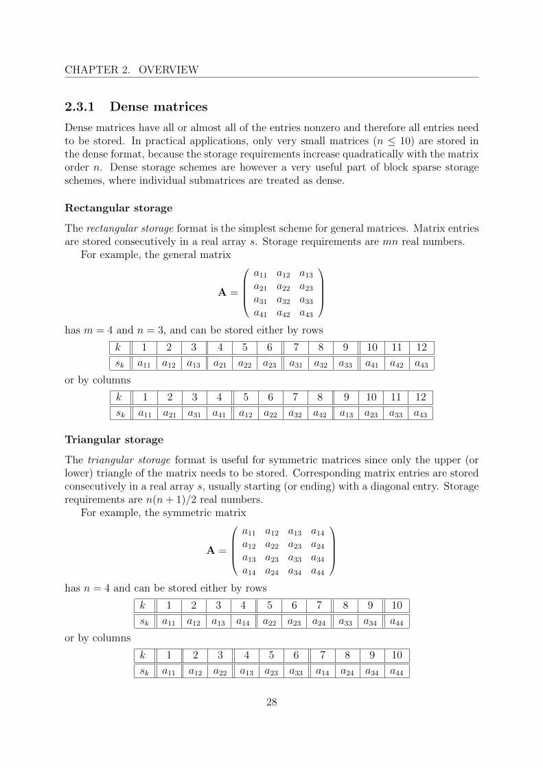
2.3.1 Dense matrices
Dense matrices have all or almost all of the entries nonzero and therefore all entries needto be stored. In practical applications, only very small matrices (n ≤ 10) are stored inthe dense format, because the storage requirements increase quadratically with the matrixorder n. Dense storage schemes are however a very useful part of block sparse storageschemes, where individual submatrices are treated as dense.
Rectangular storage
The rectangular storage format is the simplest scheme for general matrices. Matrix entriesare stored consecutively in a real array s. Storage requirements are mn real numbers.
For example, the general matrix
A =
a11 a12 a13a21 a22 a23a31 a32 a33a41 a42 a43
has m = 4 and n = 3, and can be stored either by rows
k 1 2 3 4 5 6 7 8 9 10 11 12
sk a11 a12 a13 a21 a22 a23 a31 a32 a33 a41 a42 a43
or by columns
k 1 2 3 4 5 6 7 8 9 10 11 12
sk a11 a21 a31 a41 a12 a22 a32 a42 a13 a23 a33 a43
Triangular storage
The triangular storage format is useful for symmetric matrices since only the upper (orlower) triangle of the matrix needs to be stored. Corresponding matrix entries are storedconsecutively in a real array s, usually starting (or ending) with a diagonal entry. Storagerequirements are n(n + 1)/2 real numbers.
For example, the symmetric matrix
A =
a11 a12 a13 a14a12 a22 a23 a24a13 a23 a33 a34a14 a24 a34 a44
has n = 4 and can be stored either by rows
k 1 2 3 4 5 6 7 8 9 10
sk a11 a12 a13 a14 a22 a23 a24 a33 a34 a44
or by columns
k 1 2 3 4 5 6 7 8 9 10
sk a11 a12 a22 a13 a23 a33 a14 a24 a34 a44
28
2.3. MATRIX STORAGE METHODS
2.3.2 Sparse matrices
Sparse matrices have most of the entries zero and therefore by storing only the nonzeroentries, a considerable reduction of the storage requirements can be achieved, althoughstoring some zero entries is usually inevitable.
Some sparse storage schemes require additional algorithmic and storage overhead tofacilitate the access to stored matrix entries. This overhead is however well justified sincethe storage requirements of a complex sparse storage scheme can be much lower than thatof a simple storage scheme, especially for large matrices.
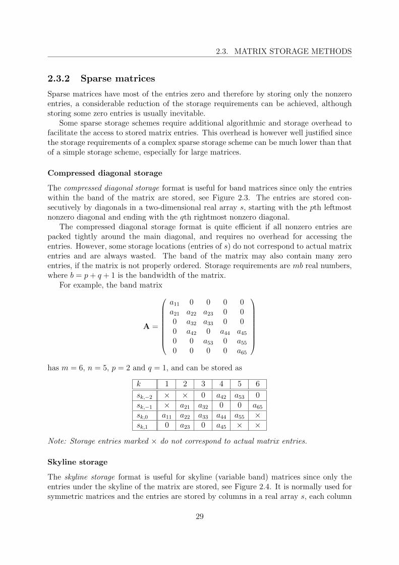
Compressed diagonal storage
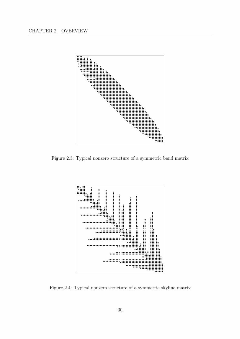
The compressed diagonal storage format is useful for band matrices since only the entrieswithin the band of the matrix are stored, see Figure 2.3. The entries are stored con-secutively by diagonals in a two-dimensional real array s, starting with the pth leftmostnonzero diagonal and ending with the qth rightmost nonzero diagonal.
The compressed diagonal storage format is quite efficient if all nonzero entries arepacked tightly around the main diagonal, and requires no overhead for accessing theentries. However, some storage locations (entries of s) do not correspond to actual matrixentries and are always wasted. The band of the matrix may also contain many zeroentries, if the matrix is not properly ordered. Storage requirements are mb real numbers,where b = p + q + 1 is the bandwidth of the matrix.
For example, the band matrix
A =
a11 0 0 0 0a21 a22 a23 0 00 a32 a33 0 00 a42 0 a44 a450 0 a53 0 a550 0 0 0 a65
has m = 6, n = 5, p = 2 and q = 1, and can be stored as
k 1 2 3 4 5 6
sk,−2 × × 0 a42 a53 0sk,−1 × a21 a32 0 0 a65sk,0 a11 a22 a33 a44 a55 ×sk,1 0 a23 0 a45 × ×
Note: Storage entries marked × do not correspond to actual matrix entries.
Skyline storage
The skyline storage format is useful for skyline (variable band) matrices since only theentries under the skyline of the matrix are stored, see Figure 2.4. It is normally used forsymmetric matrices and the entries are stored by columns in a real array s, each column
29
CHAPTER 2. OVERVIEW
Figure 2.3: Typical nonzero structure of a symmetric band matrix
Figure 2.4: Typical nonzero structure of a symmetric skyline matrix
30
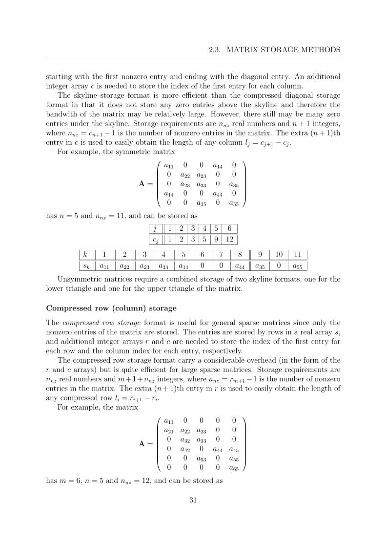
2.3. MATRIX STORAGE METHODS
starting with the first nonzero entry and ending with the diagonal entry. An additionalinteger array c is needed to store the index of the first entry for each column.
The skyline storage format is more efficient than the compressed diagonal storageformat in that it does not store any zero entries above the skyline and therefore thebandwith of the matrix may be relatively large. However, there still may be many zeroentries under the skyline. Storage requirements are nnz real numbers and n + 1 integers,where nnz = cn+1− 1 is the number of nonzero entries in the matrix. The extra (n+ 1)thentry in c is used to easily obtain the length of any column lj = cj+1 − cj.
For example, the symmetric matrix
A =
a11 0 0 a14 00 a22 a23 0 00 a23 a33 0 a35a14 0 0 a44 00 0 a35 0 a55
has n = 5 and nnz = 11, and can be stored as
j 1 2 3 4 5 6
cj 1 2 3 5 9 12
k 1 2 3 4 5 6 7 8 9 10 11
sk a11 a22 a23 a33 a14 0 0 a44 a35 0 a55
Unsymmetric matrices require a combined storage of two skyline formats, one for thelower triangle and one for the upper triangle of the matrix.
Compressed row (column) storage
The compressed row storage format is useful for general sparse matrices since only thenonzero entries of the matrix are stored. The entries are stored by rows in a real array s,and additional integer arrays r and c are needed to store the index of the first entry foreach row and the column index for each entry, respectively.
The compressed row storage format carry a considerable overhead (in the form of ther and c arrays) but is quite efficient for large sparse matrices. Storage requirements arennz real numbers and m+1+nnz integers, where nnz = rm+1−1 is the number of nonzeroentries in the matrix. The extra (n+ 1)th entry in r is used to easily obtain the length ofany compressed row li = ri+1 − ri.
For example, the matrix
A =
a11 0 0 0 0a21 a22 a23 0 00 a32 a33 0 00 a42 0 a44 a450 0 a53 0 a550 0 0 0 a65
has m = 6, n = 5 and nnz = 12, and can be stored as
31
CHAPTER 2. OVERVIEW
i 1 2 3 4 5 6 7
ri 1 2 5 7 10 12 13
k 1 2 3 4 5 6 7 8 9 10 11 12
ck 1 1 2 3 2 3 2 4 5 3 5 5sk a11 a21 a22 a23 a32 a33 a42 a44 a45 a53 a55 a65
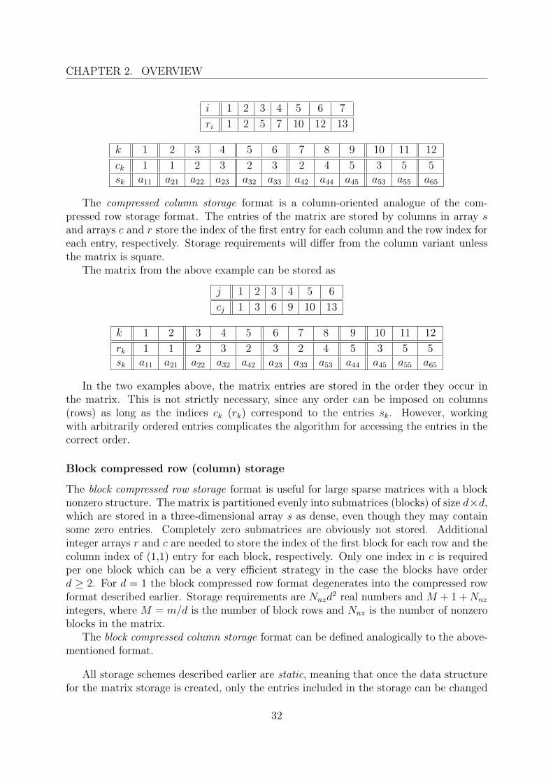
The compressed column storage format is a column-oriented analogue of the com-pressed row storage format. The entries of the matrix are stored by columns in array sand arrays c and r store the index of the first entry for each column and the row index foreach entry, respectively. Storage requirements will differ from the column variant unlessthe matrix is square.
The matrix from the above example can be stored as
j 1 2 3 4 5 6
cj 1 3 6 9 10 13
k 1 2 3 4 5 6 7 8 9 10 11 12
rk 1 1 2 3 2 3 2 4 5 3 5 5sk a11 a21 a22 a32 a42 a23 a33 a53 a44 a45 a55 a65
In the two examples above, the matrix entries are stored in the order they occur inthe matrix. This is not strictly necessary, since any order can be imposed on columns(rows) as long as the indices ck (rk) correspond to the entries sk. However, workingwith arbitrarily ordered entries complicates the algorithm for accessing the entries in thecorrect order.
Block compressed row (column) storage
The block compressed row storage format is useful for large sparse matrices with a blocknonzero structure. The matrix is partitioned evenly into submatrices (blocks) of size d×d,which are stored in a three-dimensional array s as dense, even though they may containsome zero entries. Completely zero submatrices are obviously not stored. Additionalinteger arrays r and c are needed to store the index of the first block for each row and thecolumn index of (1,1) entry for each block, respectively. Only one index in c is requiredper one block which can be a very efficient strategy in the case the blocks have orderd ≥ 2. For d = 1 the block compressed row format degenerates into the compressed rowformat described earlier. Storage requirements are Nnzd
2 real numbers and M + 1 + Nnz
integers, where M = m/d is the number of block rows and Nnz is the number of nonzeroblocks in the matrix.
The block compressed column storage format can be defined analogically to the above-mentioned format.
All storage schemes described earlier are static, meaning that once the data structurefor the matrix storage is created, only the entries included in the storage can be changed
32
2.4. DIRECT SOLVERS
and no other entries can be added. It is however possible to define dynamic block com-pressed storage format (row or column) that allows new entries to be added to the storagedata structure almost arbitrarily, which is very useful in direct methods not only for thematrix factorization, but also when the matrix is assembled submatrix-by-submatrix, forexample in the finite element method.
One of the possible approaches for symmetric matrices is to replace array r with arrayp that stores the index of the next block on the same row (column), and reserve the firstN entries in arrays p, c and s for diagonal blocks. For any block k, entry pk holds theindex of the next block in the same row or 0 if the block is the last block on the row,and entry pi holds the index of the first nondiagonal block in the row i. If the blocksare inserted into the linked lists in the ascending order of their column indices, the accessalgorithm can be much simpler (but it is not mandatory). Storage requirements are Nnzd
2
real numbers and 2Nnz integers, but in this case Nnz must be chosen suitably large toaccomodate all blocks to be added. The number of nonzero blocks in any row can beobtained either by scanning the corresponding linked list, or can be stored explicitly in aseparate array, which however increases the storage requirements by another N integers.
The dynamic block compressed row storage format of a symmetric block sparse matrixis illustrated in Figure 2.5.
There are several other possible approaches how to define a block sparse storagescheme. For example, a block sparse storage scheme called K3, which is designed specif-ically for the finite element analysis of solids and structures and implemented in C, isdescribed in [38].
2.4 Direct solvers
Direct solvers can be divided according to the used algorithms and storage schemes intodense direct solvers and sparse direct solvers. Dense direct solvers will not be discussed,since they are not suitable for the solution of finite element problems of a practical sizedue to O(n2) storage and O(n3) complexity. Furthermore, the implementation of densedirect solvers is relatively simple and straightforward.
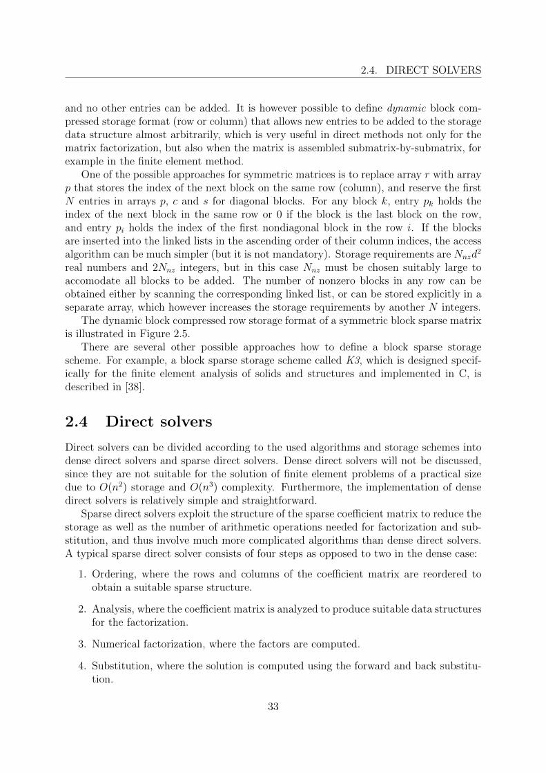
Sparse direct solvers exploit the structure of the sparse coefficient matrix to reduce thestorage as well as the number of arithmetic operations needed for factorization and sub-stitution, and thus involve much more complicated algorithms than dense direct solvers.A typical sparse direct solver consists of four steps as opposed to two in the dense case:
1. Ordering, where the rows and columns of the coefficient matrix are reordered toobtain a suitable sparse structure.
2. Analysis, where the coefficient matrix is analyzed to produce suitable data structuresfor the factorization.
3. Numerical factorization, where the factors are computed.
4. Substitution, where the solution is computed using the forward and back substitu-tion.
33
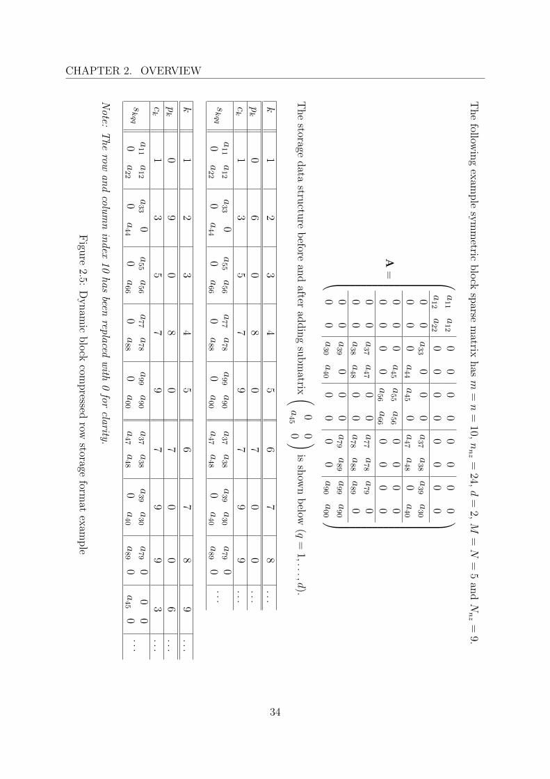
CHAPTER 2. OVERVIEWT
he
followin
gex
ample
sym
metric
blo
cksp
arsem
atrixhas
m=
n=
10,nnz
=24,
d=
2,M
=N
=5
andN
nz
=9.
A=
a11
a12
00
00
00
00
a12
a22
00
00
00
00
00
a33
00
0a37
a38
a39
a30
00
0a44
a45
0a47
a48
0a40
00
0a45
a55
a56
00
00
00
00
a56
a66
00
00
00
a37
a47
00
a77
a78
a79
00
0a38
a48
00
a78
a88
a89
00
0a39
00
0a79
a89
a99
a90
00
a30
a40
00
00
a90
a00
The
storagedata
structu
reb
eforean
dafter
addin
gsu
bm
atrix (0
0a45
0 )is
show
nb
elow(q
=1,...,d
).
k1
23
45
67
8...
pk
06
08
07
00
...ck
13
57
97
99
...
skqq
a11
a12
0a22
a33
00
a44
a55
a56
0a66
a77
a78
0a88
a99
a90
0a00
a37
a38
a47
a48
a39
a30
0a40
a79
0a89
0...
k1
23
45
67
89
...
pk
09
08
07
00
6...
ck
13
57
97
99
3...
skqq
a11
a12
0a22
a33
00
a44
a55
a56
0a66
a77
a78
0a88
a99
a90
0a00
a37
a38
a47
a48
a39
a30
0a40
a79
0a89
00
0a45
0...
Note:
The
rowan
dcolu
mn
index
10has
beenreplaced
with
0for
clarity.
Figu
re2.5:
Dynam
icblo
ckcom
pressed
rowstorage
format
exam
ple
34
2.4. DIRECT SOLVERS
Steps 1 and 2 usually involve only integer operations (graphs used in ordering andanalysis can be represented by sets of integers), whereas steps 3 and 4 involve operationson real numbers. Some steps may be combined depending on the implementation.
Ordering
Ordering produces permutation matrices P and Q, which are used to reorder the coeffi-cient matrix to allow its efficient storage. The matrix should be reordered on solver inputinstead of performing the rather impractical matrix multiplication PAQ.
The particular ordering method depends on the solver implementation; profile mini-mization orderings are best suited for skyline solvers whereas fill-in minimization orderingsare best suited for sparse solvers.
The ordering step is usually completely independent on the other steps.
Analysis
The analysis step is necessary to determine the sparsity structure of the coefficient ma-trix factors in order to allocate appropriate data structures. It can be usually performedtogether with ordering, but it is dependent on the algorithm used for numerical factor-ization.
If the coefficient matrix is positive definite, both the ordering and the analysis canbe carried out separately from the numerical factorization. Otherwise, analysis has to beperformed during the numerical factorization since it may involve pivoting for numericalstability.
Numerical factorization
Numerical factorization is the most computationally difficult part of the solution process.Generally, the decomposition PAQ = LU can be performed either by a right-looking or aleft-looking algorithm: a right-looking (eager) algorithm updates the elements/columns tothe right as soon as the current element/column has been computed, while a left-looking(lazy) algorithm updates the current element/column from earlier elements/columns aslate as possible. Both algorithms are equivalent in terms of number of arithmetic oper-ations, and the preference of one over the other depends purely on the particular solverimplementation and matrix storage used.
The factors are normally stored in place of the original coefficient matrix for maximumefficiency and minimum storage requirements, i.e., during the factorization, the entriesof the original matrix are gradually overwritten with the entries of the factors. In thesymmetric case, only a triangular part of the coefficient matrix and the factor needs tobe stored.
Substitution
The final step is the solution of the decomposed system. Since the factors are triangularor diagonal, the corresponding linear systems can be solved by a simple substitution.
35
CHAPTER 2. OVERVIEW
First, the forward substitution Ly = Pb is performed with the right-hand side (per-muted with the left permutation vector) and the lower triangular factor to obtain thereduced right-hand side. Second, the back substitution Uz = y is performed with thereduced right-hand side and the upper triangular factor to obtain the permuted solu-tion. Last, the solution vector is permuted back into the original system using the rightpermutation matrix x = Qz.
The solution in the symmetric case is analogous, however factor LT (Cholesky) orfactor DLT is used instead of factor U and permutation matrix PT instead of permutationmatrix Q.
Methods involved in dense and sparse direct solvers are discussed for example in [13],[14], [7] or [23].
2.4.1 Standard implementations
There are four basic classes of sparse direct solvers: frontal solver, skyline (or band) solver,sparse solver, and multifrontal solver.
Frontal solver
Frontal solvers are based on the frontal solution method [24, 30], which has emerged fromthe application of finite element method in structural analysis.
This method involves an auxiliary matrix, called frontal matrix, that is used to storeonly an active part of the coefficient matrix. Element matrices are added to the frontalmatrix one by one, and the elimination of a pivot is performed as soon as it is fullysummed, i.e., there are no contributions from the other elements. The eliminated rowis then moved out of the frontal matrix into the factor that is usually stored on disk.Consequently, the assembly and the factorization processes are actually interleaved, andthe coefficient matrix is never assembled explicitly.
In non-element applications, rows of the coefficient matrix (equations) are added intothe frontal matrix one by one, and a pivot is eliminated when it does not appear in anyof the remaining rows.
The frontal solution method uses a right-looking algorithm since the already eliminatedmatrix rows are moved out of core. The frontal matrix is dense, therefore the factorizationwithin the matrix can be carried out very efficiently. The size of the frontal matrix dependson the front width, i.e., the number of simultaneously processed elements (equations).The front width is affected only by the ordering of elements; ordering methods cannot beutilized since the properties of the coefficient matrix such as the profile or the sparsitypattern are irrelevant.
Frontal solvers are quite memory-efficient and are capable of solving large problems,since only the frontal matrix needs to be stored in-core. However, in the case of largeproblems, the disk storage needed for the factors is usually high, and combined with theslow disk access times the practical usability is reduced.
36
2.4. DIRECT SOLVERS
Skyline solver
Skyline solvers are based on the active column solution (skyline reduction) method [5].This method exploits the fact that the coefficient matrix always retains the same profile(skyline) throughout the factorization, i.e., the fill-in occurs only inside the profile andthe entries outside the profile remain zero. Therefore, all the storage space necessary forthe factorization can be allocated in advance.
The coefficient matrix is stored in a skyline format (by columns) and a left-lookingalgorithm is used for factorization. Since the columns are stored as dense vectors, theinnermost loops do not require indirect addressing.
A similar approach using a band format (band solvers) may be useful in some cases tosimplify the factorization algorithm at the cost of higher storage requirements and largernumber of arithmetic operations on zero elements.
Although the skyline format is more efficient than the band format, neither of them isfeasible for large problems even when a suitable profile minimization ordering is employed.
Sparse solver
Sparse solvers1 operate only on nonzero entries of the coefficient matrix and the factorsand are generally very efficient, especially for large problems, where the overhead requiredby a sparse storage scheme (for example the compressed column format) is negligible. Thisapproach requires the most complicated algorithms.
The sparse factorization can be both right-looking and left-looking, depending onthe particular matrix storage scheme chosen. An indirect addressing has to be used inthe innermost loops due to the fact that the columns (or rows) are stored as sparsevectors. Also, an efficient implementation of the fill-in is necessary; some algorithms needthe locations of the fill-in to be known in advance, whereas other algorithms allow theaddition of new nonzero entries into the matrix storage dynamically.
Ordering methods to reduce the fill-in must be employed to achieve reasonable storagerequirements and computational costs. For large problems, an out-of-core implementationis mandatory since it may not be possible, due to the fill-in, to store the whole factors inthe memory, even in the case the whole coefficient matrix can be stored.
A summary of the methods used in sparse direct solvers can be found for example in[27] or [37]. The latter work deals in detail with a particular implementation of a sparsedirect solver written in C++.
Multifrontal solver
Multifrontal solvers are based on the multifrontal solution method [16], which is an ex-tension of the frontal solution method intended for a parallel implementation on high-performance computers. This method is however efficient also on single-processor com-
1The term sparse solver sometimes means iterative solver, but in this work it always refers to a sparsedirect solver based on a sparse factorization.
37
CHAPTER 2. OVERVIEW
puters, and has lower storage requirements and computational costs than the frontalsolution method.
Instead of one frontal matrix multiple frontal matrices are used simultaneouslythroughout the factorization. For each pivot, a separate frontal matrix is created, elim-inated and maintained until it is required by another pivot in subsequent factorizationsteps. If the coefficient matrix has a block structure, it can be exploited by constructingthe frontal matrix for all pivots in a block, reducing the number of fronts and the numberof arithmetic operations needed to compute the factors. An assembly tree (similar to agraph in ordering methods) can be used to analyze and optimize the elimination and tomerge pivots in fronts.
Multifrontal solvers require more out-of-core data manipulation and more storage forfrontal matrices of smaller size than the frontal solvers. However, an important advantageis that any ordering method can be employed to reduce the storage requirements for thefactors.
2.4.2 Available software
A recent list of about 50 available sparse direct solver codes is presented in [10]. Thelist includes main features of the codes, such as used factorization method or orderingmethod, references to relevant papers and authors’ contact information. Another study,given in [23], presents a comprehensive numerical evaluation of 10 available sparse directsolvers for large linear systems.
Commercial codes are not considered since they present ‘black box’ designs with alimited extensibility, not to mention the need for expensive licenses. Also, the details ofcommercial implementations are not publicly available.
One particular exception is the PMD finite element system, which is sold commercially,but its source code is available for research purposes to co-developers.
PMD: Package for Machine Design
PMD is a full-featured platform-independent in-house code for finite element analysisof 2-D, 2.5-D and 3-D problems in elasticity, heat transfer, eigenproblems, seismicity,stability, plasticity, creep, contact, etc. It comprises of a set of command-line programs,developed in FORTRAN 77. Each program is designed to perform a part of the finiteelement computation, and several programs are used in batch depending on the type of theproblem to obtain the required solution. This modular design along with the standardizedinput and output data files allows for an easy extensibility. In the case some modifiedmethod needs to be implemented or a new method needs to be tested, either a completelynew program can be introduced, or an existing program can be replaced by a more efficientversion, both without affecting the rest of the system.
More information can be found in the PMD User Guide [33], the PMD ReferenceGuide [32] and the PMD Example Manual [31].
38
Chapter 3
Aims of the Thesis
The primary aim of this thesis is to improve methods and algorithms for the solutionof sparse linear equation systems in order to reduce the necessary requirements on com-putational time and storage space, in particular, when applied to large finite elementproblems. The focus is on the fundamental methods present in any sparse direct solutionprocess: the storage method for the coefficient matrix, the ordering method, and thesolution (factorization) method.
The secondary aim is the implementation of a sparse direct solver for finite elementanalysis in solid continuum mechanics based on the methods proposed in the theoreticalpart of this work. The code is intended to be integrated into the PMD finite elementsystem, therefore, an important part is to produce efficient implementation that can fullyreplace the existing frontal solver.
The proposed methods are restricted to symmetric positive definite linear equationsystems that are the most common in the finite element analysis of solids and structures.
To summarize, the aims of the thesis are defined as follows.
1. Based on the critical overview, propose efficient methods and algorithms suitablefor the solution of large finite element problems.
• Generalize the K3 sparse matrix storage scheme.
• Improve the minimum degree ordering algorithm.
• Improve the standard LDLT factorization algorithm.
2. Implement a sparse direct solver, laying emphasis on the effectiveness of the solutionprocess.
• Implement both the in-core and out-core version of the solver.
• Integrate the code into the PMD finite element system.
3. Perform tests and assessments of the solver.
• Use the standard problems taken from the PMD Example Manual.
39

CHAPTER 3. AIMS OF THE THESIS
• Use large finite element problems taken from real-world engineering applica-tions.
• Compare the sparse direct solver’s performace against the frontal solver.
40
Chapter 4
Applied methods
In this chapter, the theoretical background of the methods used in the work is explained.Proposed modifications and algorithms to enhance the effectiveness of the applied methodsare presented in Chapter 5.
The first three sections describe the selected matrix storage method, the orderingmethod, and the solution method, respectively. These methods form the basis of anysparse direct solver and are interdependent, meaning that the choice of one method affects(to some degree) the choice of the other methods. Even for large problems, there is nogenerally best combination of the methods since various approaches are possible. Theultimate efficiency of a sparse direct solver will always highly depend on the particularnumerical implementation. The choice of the appropriate methods is therefore a non-trivial issue.
The fourth and final section discusses several concepts and requirements of the PMDsystem that are necessary for the intended implementation of a sparse direct solver.
4.1 Matrix storage method
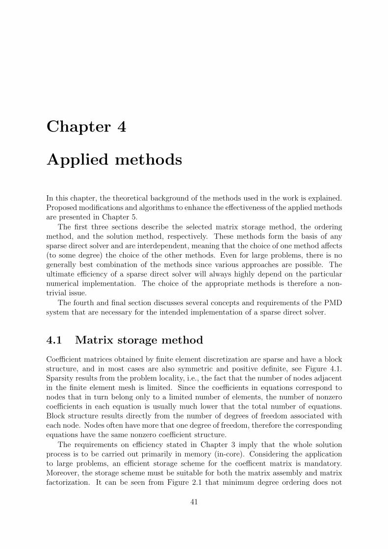
Coefficient matrices obtained by finite element discretization are sparse and have a blockstructure, and in most cases are also symmetric and positive definite, see Figure 4.1.Sparsity results from the problem locality, i.e., the fact that the number of nodes adjacentin the finite element mesh is limited. Since the coefficients in equations correspond tonodes that in turn belong only to a limited number of elements, the number of nonzerocoefficients in each equation is usually much lower that the total number of equations.Block structure results directly from the number of degrees of freedom associated witheach node. Nodes often have more that one degree of freedom, therefore the correspondingequations have the same nonzero coefficient structure.
The requirements on efficiency stated in Chapter 3 imply that the whole solutionprocess is to be carried out primarily in memory (in-core). Considering the applicationto large problems, an efficient storage scheme for the coefficent matrix is mandatory.Moreover, the storage scheme must be suitable for both the matrix assembly and matrixfactorization. It can be seen from Figure 2.1 that minimum degree ordering does not
41
CHAPTER 4. APPLIED METHODS
Note: The mesh nodes are numbered so that the frontwidth is minimal to facilitate the useof a frontal solver.
Figure 4.1: Example 3-D finite element mesh (top) and corresponding coefficient matrixstructure (bottom) for an elastostatic problem
42
4.1. MATRIX STORAGE METHOD
IndexPointer tosubmatrix
Pointer tonext item
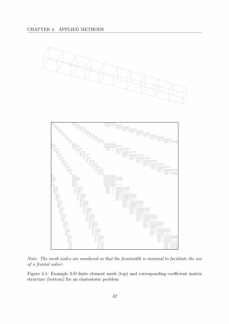
Figure 4.2: Basic element (item) of the K3 data structure
result in a band matrix, and a skyline storage format would not be efficient due to veryhigh and very sparse columns. Compressed row storage format could be used, but wouldhave unreasonably large overhead. However, a general block sparse scheme such as theblock compressed row storage format is well suited and efficient. The K3 storage formatpresents several advantages over the standard block compressed row storage format andis explained in this section in detail.
4.1.1 K3 storage format
The K3 sparse matrix storage system [38] exploits the features of newer high-level pro-gramming languages such as structured data types, pointers and dynamic memory allo-cation, to implement a convenient block sparse storage scheme for the use in the finiteelement method. It is somewhat similar to the dynamic block compressed row storageformat (see Subsection 2.3.2).
Considering a finite element mesh with N nodes, where each node has d degrees offreedom, the corresponding coefficient matrix can be partitioned evenly into N ×N nodalsubmatrices of order d. The use of the mesh topology as means for determining thepartitioning of the coefficient matrix into submatrices is advantageous since otherwise acomplicated and time-consuming algorithm would be needed to search for some nonzeroblock pattern.
After the partitioning, nonzero submatrices (i.e., submatrices with at least one nonzeroentry) are stored in the K3 data structure, which is composed of items. Each item consistsof three data members, see Figure 4.2:
1. Index. This data member stores either the nodal column index for nondiagonalitems or the number of items on the corresponding nodal row for diagonal items.
2. Pointer to submatrix. This data member stores the pointer to submatrix entriescorresponding to the nodal row and column. The submatrix is stored by rows ina rectangular dense format, or in a triangular dense format in the case of diagonalitems.
3. Pointer to next item. This data member stores the pointer to the next item in thenodal row. The items on each row are stored in a linked list that starts with thediagonal item and are sorted by ascending order of the column index. If the item isthe last item on the row, the pointer has a special null value.
The K3 data structure is created as an array of diagonal items, with all pointersinitialized to null (i.e., they do not point anywhere). The size of the array is fixed and
43
CHAPTER 4. APPLIED METHODS
known since it can be calculated easily using the number of nodes N and number of nodaldegrees of freedom d. Nondiagonal items and all submatrices are created dynamically1
and are referenced by pointers in the other items. The size of dynamically allocated datais unknown, but it is not needed due to the use of memory allocation.
Fundamental operations on the K3 data structure include accessing, update and ad-dition of an item. Addition of new items is done primarily in the assembly, but also inthe factorization, when the fill-in occurs and the corresponding item is not present in thestorage. The algorithm for assembling a nodal submatrix into the K3 data structure isdescribed below, see Table 4.1 and Figure 4.3.
Step 1 calculates the corresponding nodal row and nodal column indices p and q fromthe row and column indices of the matrix entry i and j, taking into consideration thatonly the upper triangular part of the matrix is stored, optionally swapping the indices andtransposing the submatrix. If nodal indices p and q are known the first two statementsmay be skipped.
Step 2 checks whether a diagonal submatrix is requested to see if it can be locatedimmediately in the array of diagonal items. Otherwise the appropriate row must bescanned to see whether the requested item is present.
Step 3 checks whether a new item needs to be inserted after the current item tomaintain the ascending order of column indices.
Step 4 advances to the next item on the row and checks if this item is the requesteditem. Otherwise the scanning of the row is continued.
Step 5 creates a new item and inserts it at the correct column position on the row byupdating the appropriate pointers. Corresponding diagonal item’s index data member isincremented to contain the correct number of nonzero blocks on the row.
Step 6 adds the submatrix to the current item’s submatrix, or, if current item’s pointerto submatrix is null, only assigns the reference to the submatrix.
The algorithm may be extended to access and/or update the whole matrix, for examplein the matrix factorization, in which case an outer loop over all p would be added and allsteps would be simplified to loop over all storage blocks in each row. Step 6 would be usedto perform the factorization on current item’s submatrix and step 3 would be changedto contain appropriate conditions for addition of a new storage block that represents thefill-in. In the matrix multiplication, step 5 may be completely removed and step 6 maybe used to operate on both submatrices Apq and Aqp.
It can be seen that the dynamic K3 data structure is very flexible in that it is capableof adding and even removing items2 (submatrices) from the storage on demand. It ishowever not very suitable for the use with iterative solvers or for the storage on a disk.For these cases a more conventional static data structure (a fixed array of items) can beused that reduces the number of pointers but practically eliminates the ability to add andremove items. Moreover, the size of the static data structure must be known in advance.
Storage requirements of the K3 data structure can be derived from the number ofmesh nodes N , number of nodal degrees of freedom d, number of nonzero submatrices
1Using language-specific memory allocation functions, such as malloc in C.2Removing of submatrices is important in the implementation of an out-of-core solution.
44
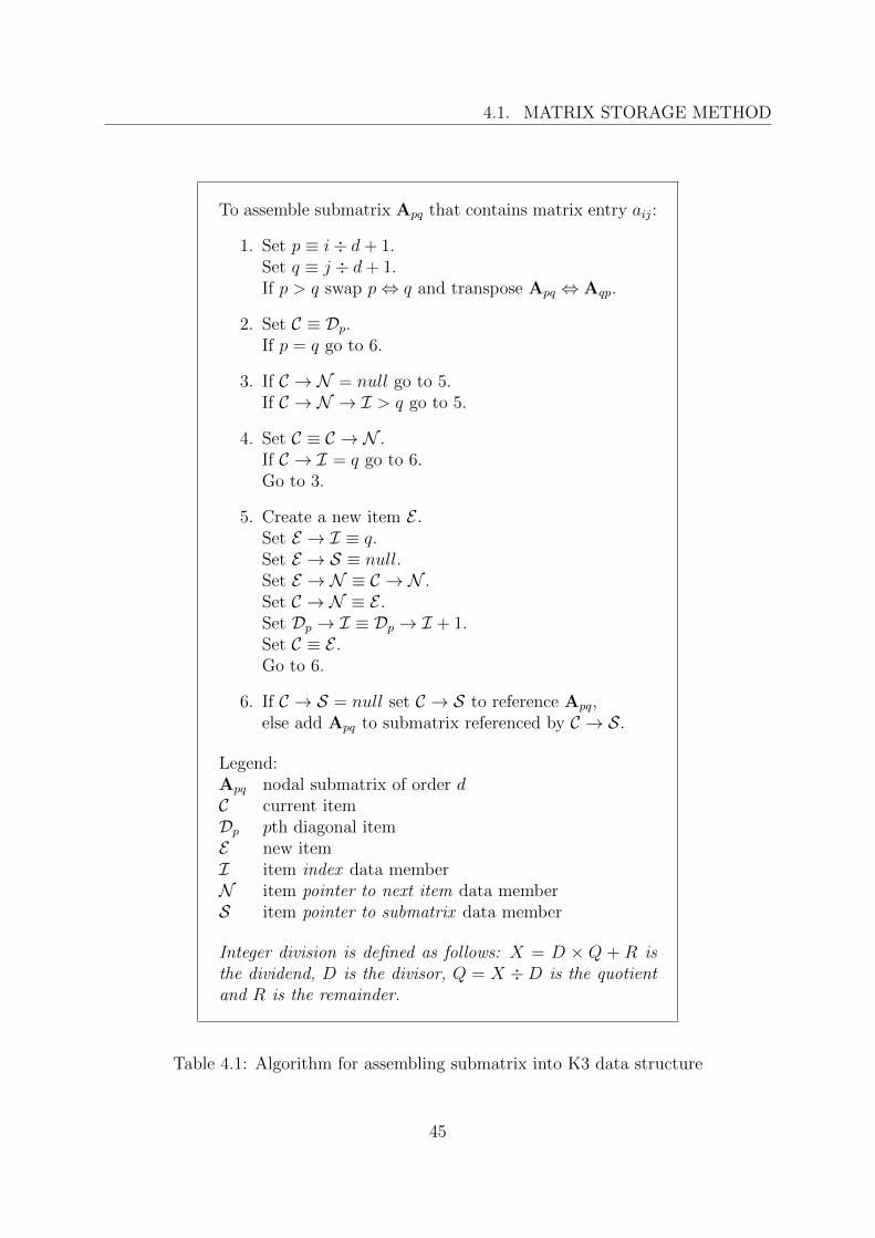
4.1. MATRIX STORAGE METHOD
To assemble submatrix Apq that contains matrix entry aij:
1. Set p ≡ i÷ d + 1.Set q ≡ j ÷ d + 1.If p > q swap p⇔ q and transpose Apq ⇔ Aqp.
2. Set C ≡ Dp.If p = q go to 6.
3. If C → N = null go to 5.If C → N → I > q go to 5.
4. Set C ≡ C → N .If C → I = q go to 6.Go to 3.
5. Create a new item E .Set E → I ≡ q.Set E → S ≡ null.Set E → N ≡ C → N .Set C → N ≡ E .Set Dp → I ≡ Dp → I + 1.Set C ≡ E .Go to 6.
6. If C → S = null set C → S to reference Apq,else add Apq to submatrix referenced by C → S.
Legend:Apq nodal submatrix of order dC current itemDp pth diagonal itemE new itemI item index data memberN item pointer to next item data memberS item pointer to submatrix data member
Integer division is defined as follows: X = D × Q + R isthe dividend, D is the divisor, Q = X ÷D is the quotientand R is the remainder.
Table 4.1: Algorithm for assembling submatrix into K3 data structure
45
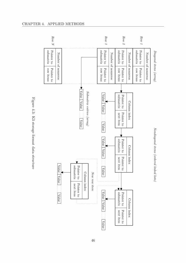
CHAPTER 4. APPLIED METHODS
Nu
mb
erof
non
zeros
Poin
terto
sub
matrix
Poin
terto
rowitem
s
Row
1
Nu
mb
erof
non
zeros
Poin
terto
sub
matrix
Poin
terto
rowitem
s
Row
2
Nu
mb
erof
non
zeros
Poin
terto
sub
matrix
Poin
terto
rowitem
s
Row
3
Nu
mb
erof
non
zeros
Poin
terto
sub
matrix
Poin
terto
rowitem
s
Row
N
Colu
mn
ind
ex
Poin
terto
sub
matrix
Poin
terto
nex
titem
Valu
eV
alue
Valu
e
Colu
mn
ind
ex
Poin
terto
sub
matrix
Poin
terto
nex
titem
Valu
eV
alu
eV
alue
Colu
mn
ind
ex
Poin
terto
sub
matrix
Poin
terto
nex
titem
Valu
eV
alue
Valu
e
Colu
mn
ind
ex
Poin
terto
sub
matrix
Poin
terto
nex
titem
Valu
eV
alue
Valu
e
Diagonalitem
s(arra
y)Nondiagonalitem
s(ordered
linked
lists)
New
row
item
Valu
eV
alue
Valu
e
Subm
atrix
entries
(arra
y)
Figu
re4.3:
K3
storageform
atdata
structu
re
46
4.2. ORDERING METHOD
(number of items) Nnz, and the size of integer, real, and pointer data types for a givencomputer platform, and have the form
L = Nnz × |integer|+ 2Nnz × |pointer|+(Nd(d + 1)
2+ (Nnz −N)d2
)× |real|. (4.1)
Equation (4.1) cannot be evaluated until the number of items Nnz is known, which isnormally only after adding all of the items. A distinct advantage of the K3 storageformat is that it does not require the storage requirements nor the indices of nonzerosubmatrices to be known in advance due to the use of memory allocation. Therefore,both the matrix assembly and the matrix factorization can be performed without theneed for the computationally expensive fill-in analysis.
Although the K3 storage format is meant for finite element meshes with a constantnumber of nodal degrees of freedom d, it can be used for variable d as well. If all nodalsubmatrices are padded with zero entries to match the largest d, the K3 storage formatcan be used exactly as described earlier, but the efficiency will be affected by the addednonzeros.
Finally, it should be noted that memory allocation is not available in older program-ming languages, such as FORTRAN,3 and therefore can present a significant problem forthe application of the K3 storage format if the use of such language is mandatory.
4.2 Ordering method
The ordering (also called reordering, preordering, renumbering, relabeling, pivoting orpermutation, depending on the context) of a matrix means switching rows and columnsof the matrix to obtain a different, preferably more suitable, order of pivots on the maindiagonal. Since switching of rows or columns is an elementary matrix operation, it doesnot change the solution of the associated linear equation system. However, the order ofunknowns is generally changed (they are relabeled), and the actual numerical implemen-tation must take trace of this relabeling to produce the solution vector in the correct(original) order.
The ordering is commonly used in the sparse matrix factorization prior to the forwardelimination (called preordering) to reduce the fill-in. Another common application of theordering (called pivoting) is to improve the numerical stability in the factorization ofindefinite matrices.
Let A be an invertible matrix, P the corresponding (left) permutation matrix and Qthe corresponding (right) permutation matrix that represent the chosen ordering of rowsand columns, respectively. Then the LU factorization (2.3) with preordering takes theform
PAQ = LU. (4.2)
3Prior to Fortran 90 standard.
47
CHAPTER 4. APPLIED METHODS
The forward substitution (2.6) takes the form
Ly = Pb (4.3)
and the back substitution (2.7) takes the form
Uz = y, (4.4)
where an additional step is needed to permute the solution back into the original orderingin the form
x = Qz. (4.5)
If matrix A is symmetric, thenQ = PT, (4.6)
U = DLT, (4.7)
and the LDLT factorization (2.11) with preordering is obtained.
The choice of the ordering method depends on the used matrix storage method andfactorization method. Although sparse factorization can utilize any ordering method, fill-in minimization is mandatory in practice to reduce storage requirements of the matrixfactors. The minimum degree algorithm is one of the most widely used orderings due toits effectiveness on a wide range of matrices. Only recently a theoretically superior butcomputationally expensive ordering method of nested dissections has been shown to bemore efficient that minimum degree in some practical cases. However, nested dissectionswill not be considered in this work.
4.2.1 Minimum degree algorithm
The minimum degree algorithm is a symmetric analogue of the Markowitz’ method [29]and was first proposed by Tinney and Walker [35] as algorithm S2. It was not renamedto minimum degree until later by Rose [34], who developed a graph theoretical model ofthe algorithm. In the past four decades, the algorithm has received much attention anda considerable amount of work has been directed towards improving the effectiveness ofits numerical implementation. The most important work include that of George and Liu[19, 20], Duff and Reid [17], the multiple minimum degree (MMD) of Liu [28] and theapproximate minimum degree (AMD) of Amestoy, Davis and Duff [1, 2].
The minimum degree algorithm analyzes the nonzero structure of a symmetric sparsematrix A to produce a permutation matrix P such that the factorization of the reordered
matrix A = PAPT
exhibits the least fill-in. Unfortunately, the problem of finding theminimum fill-in is NP-complete, therefore the minimum degree algorithm is actually onlyone of the possible heuristics.
The description of the minimum degree algorithm relies heavily on the theory ofgraphs, that is briefly mentioned in Section 2.2, and is explained in detail for example in[11].
48
4.2. ORDERING METHOD
Elimination graph
The original minimum degree algorithm is based on the symbolic elimination using theelimination graph of the matrix. Considering an n× n matrix A, the initial graph G0 =(V0, E0) is constructed according to the nonzero structure of the matrix, where the vertexset V0 = {1, . . . , n} and the edge set E0 = {(i, j) : aij 6= 0∧ i 6= j}. Since the matrix A issymmetric, the resulting graph G0 is undirected and simple.
The symbolic elimination proceeds in steps that simulate the actual numerical elim-ination (factorization). In the kth elimination step, vertex p corresponding to the kthpivot is removed from the graph Gk−1 = (Vk−1, Ek−1), i.e., vertex p is removed from Vk−1to form the new set Vk and all edges (i, p) are removed from Ek−1 to form the new set Ek.Then new edges (i, j) are added to Ek for all i, j adjacent to p in Gk−1. In other words,new edges are added to the graph to connect all vertices formerly connected to vertex p,creating a clique (a fully connected subgraph). This addition of edges to the graph Gk
represents the fill-in created in the kth step of the numerical factorization and means thatthe storage requirements of the elimination graph cannot be known in advance.
The minimum degree algorithm selects the pivot p in the kth step of the symbolicelimination that has a minimum degree, defined by
tp = |AdjGk−1(p)|. (4.8)
Selecting p as the kth pivot causes the addition of at most (t2p − tp)/2 new edges in Gk.The permutation matrix P is obtained from the sequence in which the vertices pk,
k = 1, . . . , n, were removed from the graph G, i.e., from the sequence of the selectedpivots.
Quotient graph
The quotient graph (also referred to as generalized element model) presents a substantialadvantage over the elimination graph, since its storage requirements never exceed the sizeof the initial graph G0.
The quotient graph Gk = (Vk∪V k, Ek∪Ek) comprises of two distinct types of verticesand edges. The vertices consist of variables Vk and elements V k, where variables arevertices that have not yet been eliminated from the graph and elements are vertices thathave been already eliminated. The edges consist of edges between variables Ek and edgesbetween variables and elements Ek. There are no edges between elements since they areunnecessary. In the initial graph G0, the sets V0 and E0 are identical to the eliminationgraph G0, and the sets V 0 and E0 are empty, i.e., G0 = G0.
The subscript k denoting the elimination step will be dropped onwards for clarity. LetAi be the set of variables adjacent to variable i in G, let Ei be the set of elements adjacentto variable i in G, and let Le be the set of variables adjacent to element e in G. Then
Ai = {j : (i, j) ∈ E}, (4.9)
Ei = {e : (i, e) ∈ E}, (4.10)
49
CHAPTER 4. APPLIED METHODS
Le = {i : (i, e) ∈ E}, (4.11)
and the adjacency sets areAdjG(i) = Ai ∪ Ei, (4.12)
AdjG(e) = Le. (4.13)
The set of variables adjacent to variable i in G, necessary for the computation of thedegree (4.8), can be obtained using equations (4.9) to (4.13), and has the form
AdjG(i) =
Ai ∪⋃e∈EiLe
\ {i}. (4.14)
The symbolic elimination proceeds similarly as with the elimination graph. The quo-tient graph is actually represented using the sets A, E and L, which is considerably moreefficient than using the sets V , V , E and E. When variable p is selected as the kthpivot, the set Lp = AdjG(p) is found using equation (4.14). An important implication ofequation (4.14) is that all variables adjacent to an element e ∈ Ep are also adjacent to theelement p, i.e., Le \ {p} ⊆ Lp. The elements e ∈ Ep are therefore no longer needed andare absorbed into the new element p. The graph is updated in the following way: first,the absorbed elements e ∈ Ep are deleted from all sets Ei, and the new element p is addedto the sets Ei for all variables i ∈ Lp. Next, the sets Ap, Ep and Le for all elements e ∈ Epare deleted. Finally, any entry j in Ai, where both i and j are in Lp, is redundant and isdeleted. This results in that the graph Gk takes the same, or less, storage than the graphGk−1, or formally
(|Ai|+ |Ei|+ |Le|)k ≤ (|Ai|+ |Ei|+ |Le|)k−1 . (4.15)
The set Lp represents the unpermuted nonzero structure of the kth column (or row) ofthe factor L, i.e., the factor entry lik will be nonzero only if i ∈ Lp. Therefore, the exactnonzero structure of the factor L (that also includes the fill-in) can be fully determinedin the course of the symbolic elimination and used for example to create appropriate datastructures for the numerical factorization.
An important property that allows the symbolic elimination algorithm to take advan-tage of graph cliques is the indistinguishability. Variables i and j are indistinguishable inG if
AdjG(i) ∪ {j} = AdjG(j) ∪ {i}, (4.16)
which also implies they have the same degree. If i is selected as pivot in step k, j can beselected in step k + 1 without causing any additional fill-in.
Let Si be the set of indistinguishable variables labeled by its principal variable i. Then
Si = {i} ∪ {j : AdjG(i) ∪ {j} = AdjG ∪ {i}} (4.17)
represents the supervariable i. Any variable from Si can be used as a principal variable forlabeling the supervariable. Variable i where Si = {i} is called simple variable. Therefore,all variables in the graph can be considered principal variables.
50
4.2. ORDERING METHOD
In the initial graph G0, all variables are simple variables. When variable p is selectedas the kth pivot, all variables in the set Sp are selected as well. The set Sp is deleted andsupervariables are identified and created. When supervariable q is created, the set Sq isfound using equation (4.17), and the sets Ai, Ei and Si for all variables i ∈ Sq \ {q} aredeleted. In practice, the indistinguishability is checked in G rather than in G, since it isfaster although some identifications may be missed. Also, only variables in Lp are checkedfor indistinguishability in each elimination step.
Selecting all variables in Sp in one step is called mass elimination and it substantiallyreduces the number of elimination steps necessary to obtain the ordering. Consequently,ordering time is reduced as well as the storage required for the quotient graph.
The external degree of a principal variable i is
di = ti − |Si|+ 1 = |AdjG(i) \ Si| = |Ai \ Si|+
∣∣∣∣∣∣ ⋃
e∈EiLe
\ Si∣∣∣∣∣∣ , (4.18)
where ti is the true degree defined by (4.8). Selecting the pivot with minimum externaldegree tends to produce a better ordering than selecting the pivot with minimum truedegree, therefore, only the use of external degrees is assumed further on.
Degree computations are the most costly part of the minimum degree algorithm due tothe presence of term
⋃e∈Ei Le, which is complicated to evaluate. In practice, the degrees
of all variables are computed in graph G0, and subsequently updated only for variables iadjacent to the pivot p in the actual step of the symbolic elimination, i.e., for variablesi ∈ Lp. This, along with the use of supervariables, results in a considerable reduction ofthe number of degree computations.
A minimum degree algorithm based on the quotient graph and including elementabsorption, mass elimination, supervariables, and external degrees is summarized in Ta-ble 4.2.
Approximate degree
An approximate degree replaces equation (4.18) with a less complex equation that com-putes an upper bound of the degree instead of the exact degree. While the cost of thedegree computation is reduced, the ordering obtained by using approximate degrees isgenerally worse (results in more fill-in) than the ordering obtained by using exact degrees.Several approximate degrees are explained next in order from the least accurate.
The approximate degree proposed by Gilbert, Moler and Schreiber [22] is
di = |Ai \ Si|+∑e∈Ei|Le \ Si|. (4.19)
The redundancy of the entries in sets Le is neglected in equation (4.19), therefore theupper bound can be computed very fast but results in a very coarse upper bound of theexact degree.
51
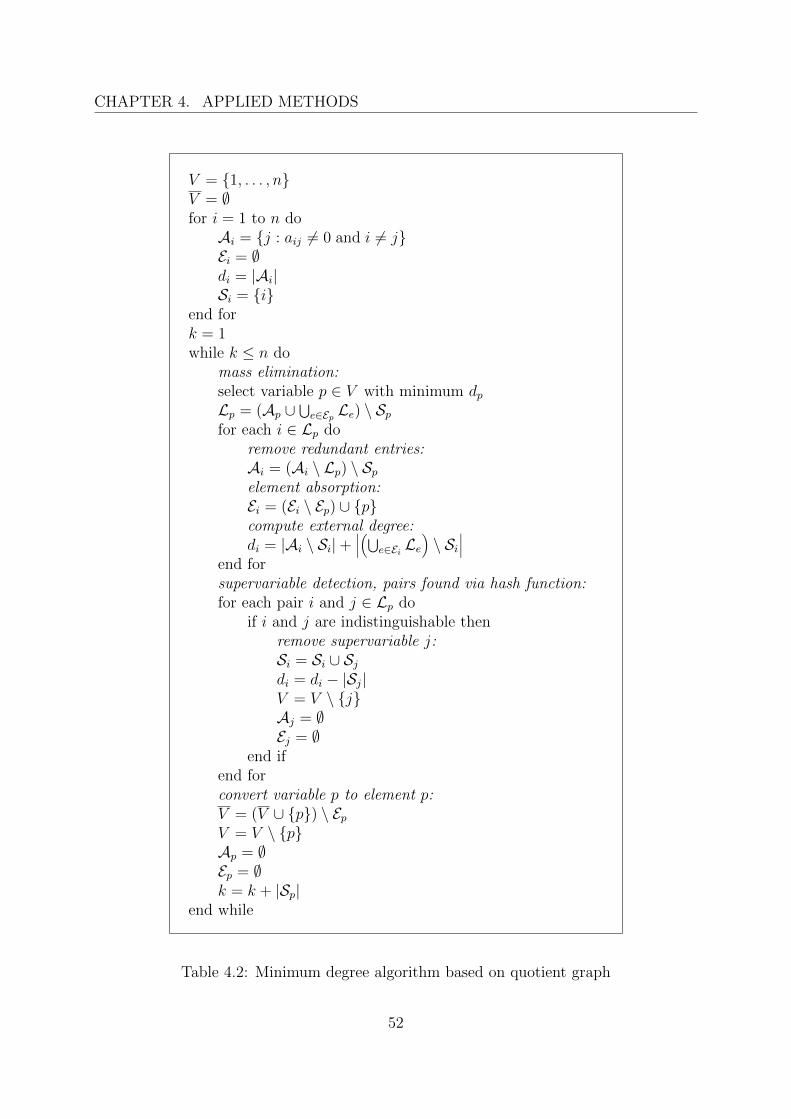
CHAPTER 4. APPLIED METHODS
V = {1, . . . , n}V = ∅for i = 1 to n doAi = {j : aij 6= 0 and i 6= j}Ei = ∅di = |Ai|Si = {i}
end fork = 1while k ≤ n do
mass elimination:select variable p ∈ V with minimum dpLp = (Ap ∪
⋃e∈Ep Le) \ Sp
for each i ∈ Lp doremove redundant entries:Ai = (Ai \ Lp) \ Spelement absorption:Ei = (Ei \ Ep) ∪ {p}compute external degree:di = |Ai \ Si|+
∣∣∣(⋃e∈Ei Le
)\ Si
∣∣∣end forsupervariable detection, pairs found via hash function:for each pair i and j ∈ Lp do
if i and j are indistinguishable thenremove supervariable j:Si = Si ∪ Sjdi = di − |Sj|V = V \ {j}Aj = ∅Ej = ∅
end ifend forconvert variable p to element p:V = (V ∪ {p}) \ EpV = V \ {p}Ap = ∅Ep = ∅k = k + |Sp|
end while
Table 4.2: Minimum degree algorithm based on quotient graph
52
4.2. ORDERING METHOD
The approximate degree proposed by Ashcraft, Eisenstat and Lucas [2] is
di =
{di if |Ei| = 2
di if |Ei| 6= 2. (4.20)
The reasoning behind equation (4.20) is that many variables are adjacent to two or fewerelements when their degree is recomputed. Utilizing the exact degree increases the com-plexity but a significantly better upper bound of the exact degree is obtained than us-ing (4.19).
The approximate degree proposed by Amestoy, Davis and Duff [2] is
di = |Ai \ Si|+ |Lp \ Si|+∑
e∈Ei\{p}|Le \ Lp|. (4.21)
In equation (4.21) the properties of subsets Le ∩ Lp and Le \ Lp are exploited to obtaina closer upper bound of the exact degree while maintaining a reasonable complexity.However, some redundant entries in sets Le are still counted.
Since the approximate degree is an upper bound of the exact degree, it cannot exceedthe number of variables in the actual elimination step n − k nor the worst case fill-in,that can be easily obtained by adding |Lp \ Si| to the degree computed in the previouselimination step. Therefore the complete form of equation (4.21) in the kth eliminationstep is
(di)k = min
n− k
(di)k−1 + |Lp \ Si||Ai \ Si|+ |Lp \ Si|+
∑e∈Ei\{p}
|Le \ Lp|
. (4.22)
The aproximate degree of Gilbert, Moler and Schreiber can be complemented in the sameway, replacing the last row in equation (4.22) with equation (4.19).
Further enhancements
Actual implementations of the minimum degree algorithm include the following enhance-ments in addition to those already mentioned: aggressive absorption, multiple eliminationand incomplete degree update.
In aggressive absorption, any element with Le \ Lp = ∅ is absorbed into element p,even if it is not adjacent to p. Aggressive absorption can improve the computation ofdegrees since it reduces the size of sets Ei.
In multiple elimination, all independent pivots with minimum degree are selectedbefore any degrees are updated. If a variable is adjacent to two or more pivot elements,its degree is computed only once.
Finally, in incomplete degree update, the degree update of an outmatched variable j isavoided until variable i is selected as pivot. Variable j is outmatched if AdjG(i) ⊆ AdjG(j).
53
CHAPTER 4. APPLIED METHODS
Tiebreaking
A crucial aspect of the minimum degree algorithm is the tiebreaking strategy that isapplied when more than one variable with minimum degree can be selected as pivot. Thematter has been a topic of research, but so far no significant method has been developed,and no established implementation of the minimum degree ordering uses tiebreaking.4
The difficulty lies mainly in the complexity of such methods, since the tiebreaking usuallyconsiderably increases the time of the symbolic elimination. Therefore, ties are resolvedgenerally by simply selecting the pivot with the lowest vertex number, which does notaffect the ordering time.
More on tiebreaking strategies can be found in [19] and [8]. For example, George andLiu suggest in [19] to apply the minimum degree algorithm to the matrix that has been‘preordered’ using the reverse Cuthill-McKee ordering (see Section 2.2). This particularprocedure is claimed to result in an ordering that is independent on the initial orderingof matrix elements, effectively resolving the ties.
4.3 Solution method
Similarly to the matrix storage method, the solution method must meet the requirementsstated in Chapter 3 that the whole solution process is to be carried out by a direct method,preferably in memory (in-core). Another requirement is that the coefficient matrices arerestricted to be symmetric and positive definite, which is a reasonable assumption for thegiven application to the finite element analysis of solids and structures.
The frontal solution method has relatively low memory demands, but it requires alot of out-of-core data manipulation that would slow down the solution considerably, andparticularly it cannot take advantage of sparse matrix ordering.
The multifrontal solution method is able to exploit ordering, but it introduces evenmore out-of-core data manipulation than the frontal solution method and involves rathercomplicated algorithms.
The active column solution (skyline reduction) method allows a complete in-core solu-tion, but requires the skyline storage format that would be very inefficient since it wouldexhibit an excessive number of unused zero entries due to very high and very sparsecolumns caused by the minimum degree ordering (see Figure 2.1 and Subsection 4.2.1).This would not be resolved even if some block variant of the skyline storage would beintroduced.
Finally, the (block) sparse direct solution method is relatively straightforward, allowsa complete in-core solution to be used, and an efficient (block) sparse matrix storagescheme and fill-in minimization ordering to be applied. It has however relatively highstorage requirements because the whole coefficient matrix has to be stored in memoryunless an out-of-core solution is considered.
4Strictly speaking, multiple elimination can be considered a somewhat limited form of tiebreaking.
54
4.3. SOLUTION METHOD
Direct solution methods based on LU, LDLT and Cholesky factorizations, that werebriefly described in Subsection 2.1.1, are all variants of the Gaussian elimination. TheGaussian elimination is a very important algorithm since it can be used to solve sys-tem (2.1) without the need for computing the inverse A−1.
4.3.1 Symmetric block sparse factorization
Standard Gaussian elimination comprises of a forward elimination, where matrix A isreduced to an upper triangular matrix along with the right-hand side vector b,5 and aback substitution, where the solution vector x is computed from the triangular systemobtained in the forward elimination. However, often the solution of the same linearequation system is required to be computed for several different right-hand sides, forexample in the finite element method, the problem may be solved for several differentloading states. The Gaussian elimination is not suitable for such cases since both theforward elimination and back substitution would be performed for each different right-hand side, which would be very inefficient due to the high computational complexity ofthe forward elimination. Therefore in practical applications, factorization methods thatseparate the reduction of the right-hand side from the reduction of the coefficient matrixitself are used. These methods allow the forward elimination to be carried out only oncefor a given system and then any number of right-hand sides may be used to compute thecorresponding solution. Consequently, the solution is divided into two steps: a forwardsubstitution, that reduces the right-hand side, and the aforementioned back substitution.6
Factorization
The forward elimination (also called reduction, triangularization, factorization or decom-position, depending on the context) of an n× n matrix A is performed in n− 1 steps.
In the kth elimination step, all column entries aik under the diagonal entry akk, calledthe pivot, are eliminated (zeroed) by subtracting a multiple of the kth row, called thepivot row, from remaining (uneliminated) rows. The multiplier for ith row is
l(k)ik = −a
(k)ik
a(k)kk
, (4.23)
where i = k + 1, . . . , n is the row index and the superscript k = 1, . . . , n− 1 refers to theactual elimination step.
5The elimination is usually done on an augmented matrix (A|b).6The term back substitution is often inaccurately used to refer to both the forward and back substi-
tution, although they are technically different.
55
CHAPTER 4. APPLIED METHODS
The kth elimination step can be written using equation (4.23) in the matrix form
Ak+1 = L−1k Ak =
=
1 0. . .
1
−a(k)k+1,k
a(k)kk
1
.... . .
0 −a(k)nk
a(k)kk
0 1
a(k)11 · · · a
(k)1k · · · a
(k)1n
. . ....
...
a(k)kk · · · a
(k)kn
a(k)k+1,k · · · a
(k)k+1,n
......
0 a(k)nk · · · a(k)nn
,
(4.24)
where Ak and Ak+1 is the partially reduced matrix in the kth and (k + 1)th eliminationstep, respectively, and Lk is the elementary matrix for elimination of the kth row.
After writing down all steps of the forward elimination the resulting matrix form is
U = An = L−1n−1 · · ·L−12 L−11 A = L−1A, (4.25)
where U is an upper triangular matrix containing the result of the forward elimination,the reduced matrix A, and L−1 is a unit lower triangular matrix, since the multiplicationof unit lower triangular matrices L−1k results in a unit lower triangular matrix. MatrixL−1 can be used to perform the forward elimination on matrix A in a single step.
Combining the leftmost and the rightmost side of (4.25) and realizing that the in-verse of a unit lower triangular matrix is also a unit lower triangular matrix, the LUfactorization of matrix A is obtained in the form
A = LU. (4.26)
Matrix U can be also expressed as a multiplication of a diagonal matrix D and a unitupper triangular matrix U. Substituting to (4.26) yields
A = LDU. (4.27)
If matrix A is symmetric, the right-hand side of (4.27) must also be symmetric, therefore
U = LT (4.28)
and hence the LDLT factorization of the matrix A is obtained in the form
A = LDLT. (4.29)
The matrix factors L and U are computed using Gaussian elimination and stored inplace of the original matrix A. In the case of a symmetric matrix A, there are two possibleapproaches how to compute the factors L and D.
56
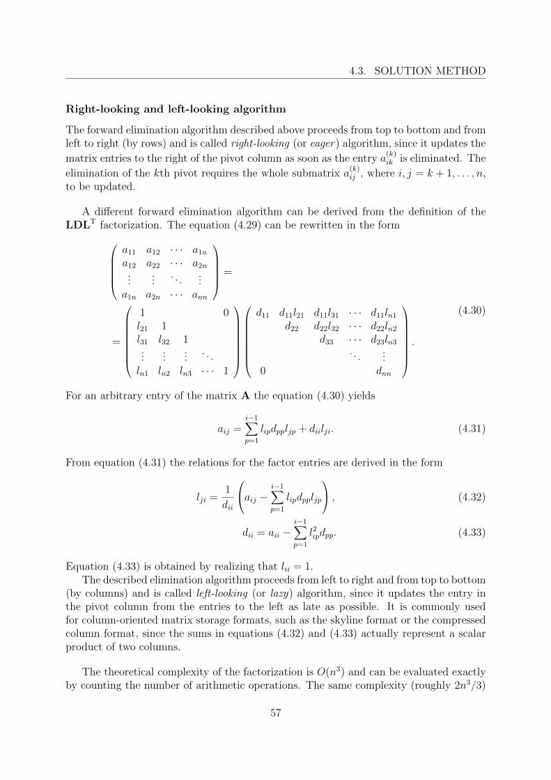
4.3. SOLUTION METHOD
Right-looking and left-looking algorithm
The forward elimination algorithm described above proceeds from top to bottom and fromleft to right (by rows) and is called right-looking (or eager) algorithm, since it updates the
matrix entries to the right of the pivot column as soon as the entry a(k)ik is eliminated. The
elimination of the kth pivot requires the whole submatrix a(k)ij , where i, j = k + 1, . . . , n,
to be updated.
A different forward elimination algorithm can be derived from the definition of theLDLT factorization. The equation (4.29) can be rewritten in the form
a11 a12 · · · a1na12 a22 · · · a2n...
.... . .
...a1n a2n · · · ann
=
=
1 0l21 1l31 l32 1...
......
. . .
ln1 ln2 ln3 · · · 1
d11 d11l21 d11l31 · · · d11ln1d22 d22l32 · · · d22ln2
d33 · · · d23ln3. . .
...0 dnn
.
(4.30)
For an arbitrary entry of the matrix A the equation (4.30) yields
aij =i−1∑p=1
lipdppljp + diilji. (4.31)
From equation (4.31) the relations for the factor entries are derived in the form
lji =1
dii
aij − i−1∑p=1
lipdppljp
, (4.32)
dii = aii −i−1∑p=1
l2ipdpp. (4.33)
Equation (4.33) is obtained by realizing that lii = 1.The described elimination algorithm proceeds from left to right and from top to bottom
(by columns) and is called left-looking (or lazy) algorithm, since it updates the entry inthe pivot column from the entries to the left as late as possible. It is commonly usedfor column-oriented matrix storage formats, such as the skyline format or the compressedcolumn format, since the sums in equations (4.32) and (4.33) actually represent a scalarproduct of two columns.
The theoretical complexity of the factorization is O(n3) and can be evaluated exactlyby counting the number of arithmetic operations. The same complexity (roughly 2n3/3)
57
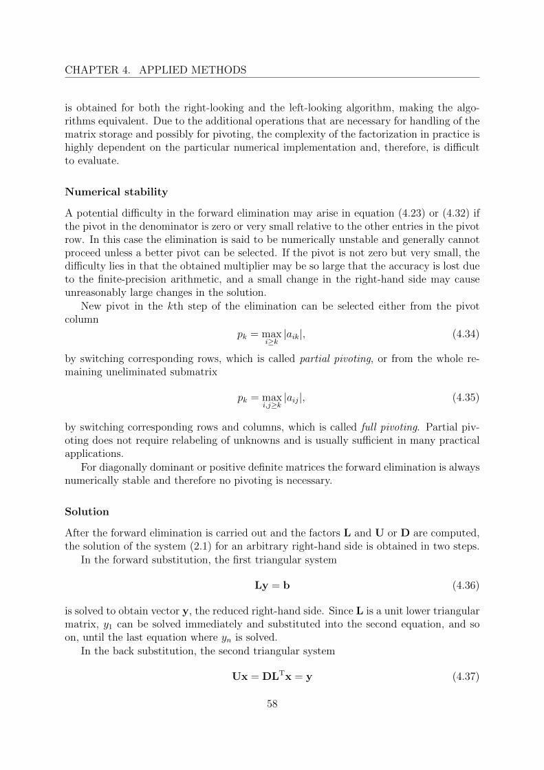
CHAPTER 4. APPLIED METHODS
is obtained for both the right-looking and the left-looking algorithm, making the algo-rithms equivalent. Due to the additional operations that are necessary for handling of thematrix storage and possibly for pivoting, the complexity of the factorization in practice ishighly dependent on the particular numerical implementation and, therefore, is difficultto evaluate.
Numerical stability
A potential difficulty in the forward elimination may arise in equation (4.23) or (4.32) ifthe pivot in the denominator is zero or very small relative to the other entries in the pivotrow. In this case the elimination is said to be numerically unstable and generally cannotproceed unless a better pivot can be selected. If the pivot is not zero but very small, thedifficulty lies in that the obtained multiplier may be so large that the accuracy is lost dueto the finite-precision arithmetic, and a small change in the right-hand side may causeunreasonably large changes in the solution.
New pivot in the kth step of the elimination can be selected either from the pivotcolumn
pk = maxi≥k|aik|, (4.34)
by switching corresponding rows, which is called partial pivoting, or from the whole re-maining uneliminated submatrix
pk = maxi,j≥k|aij|, (4.35)
by switching corresponding rows and columns, which is called full pivoting. Partial piv-oting does not require relabeling of unknowns and is usually sufficient in many practicalapplications.
For diagonally dominant or positive definite matrices the forward elimination is alwaysnumerically stable and therefore no pivoting is necessary.
Solution
After the forward elimination is carried out and the factors L and U or D are computed,the solution of the system (2.1) for an arbitrary right-hand side is obtained in two steps.
In the forward substitution, the first triangular system
Ly = b (4.36)
is solved to obtain vector y, the reduced right-hand side. Since L is a unit lower triangularmatrix, y1 can be solved immediately and substituted into the second equation, and soon, until the last equation where yn is solved.
In the back substitution, the second triangular system
Ux = DLTx = y (4.37)
58
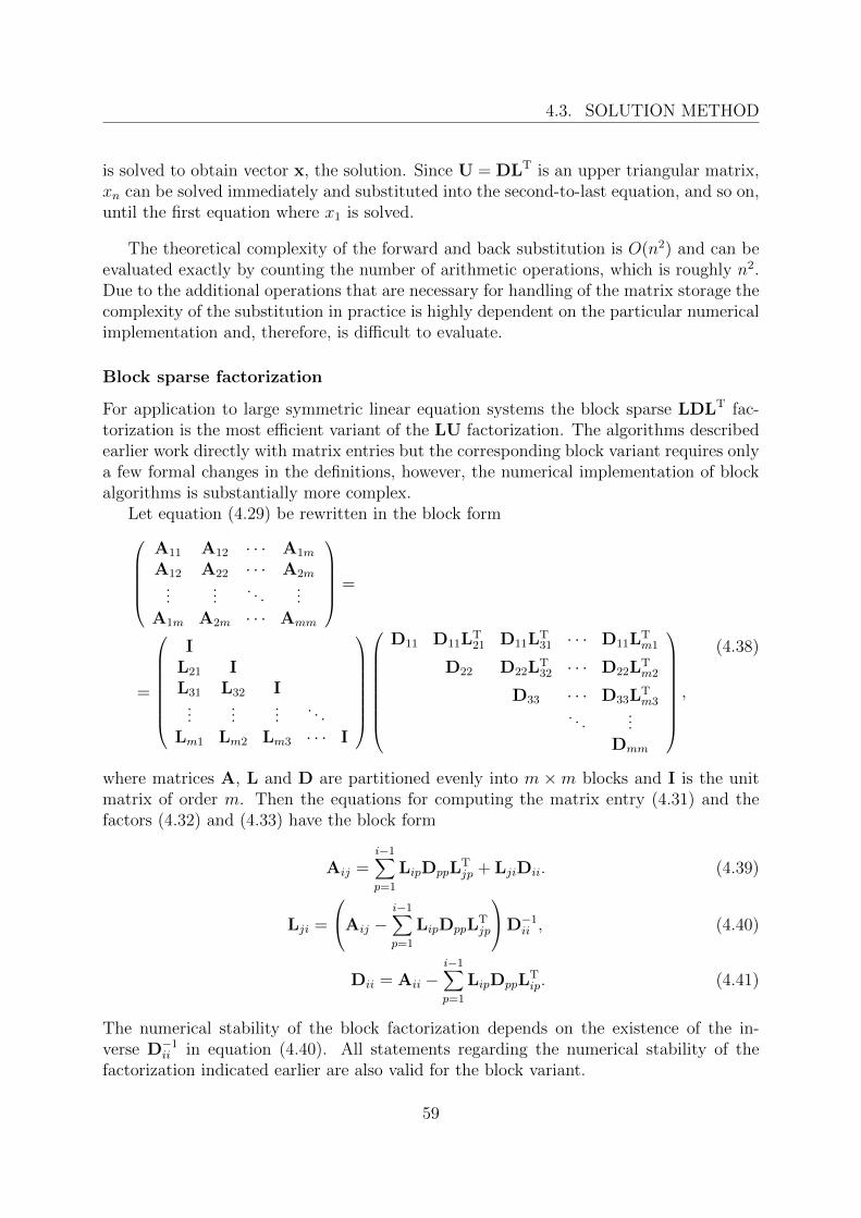
4.3. SOLUTION METHOD
is solved to obtain vector x, the solution. Since U = DLT is an upper triangular matrix,xn can be solved immediately and substituted into the second-to-last equation, and so on,until the first equation where x1 is solved.
The theoretical complexity of the forward and back substitution is O(n2) and can beevaluated exactly by counting the number of arithmetic operations, which is roughly n2.Due to the additional operations that are necessary for handling of the matrix storage thecomplexity of the substitution in practice is highly dependent on the particular numericalimplementation and, therefore, is difficult to evaluate.
Block sparse factorization
For application to large symmetric linear equation systems the block sparse LDLT fac-torization is the most efficient variant of the LU factorization. The algorithms describedearlier work directly with matrix entries but the corresponding block variant requires onlya few formal changes in the definitions, however, the numerical implementation of blockalgorithms is substantially more complex.
Let equation (4.29) be rewritten in the block formA11 A12 · · · A1m
A12 A22 · · · A2m...
.... . .
...A1m A2m · · · Amm
=
=
IL21 IL31 L32 I
......
.... . .
Lm1 Lm2 Lm3 · · · I
D11 D11LT21 D11L
T31 · · · D11L
Tm1
D22 D22LT32 · · · D22L
Tm2
D33 · · · D33LTm3
. . ....
Dmm
,
(4.38)
where matrices A, L and D are partitioned evenly into m ×m blocks and I is the unitmatrix of order m. Then the equations for computing the matrix entry (4.31) and thefactors (4.32) and (4.33) have the block form
Aij =i−1∑p=1
LipDppLTjp + LjiDii. (4.39)
Lji =
Aij −i−1∑p=1
LipDppLTjp
D−1ii , (4.40)
Dii = Aii −i−1∑p=1
LipDppLTip. (4.41)
The numerical stability of the block factorization depends on the existence of the in-verse D−1ii in equation (4.40). All statements regarding the numerical stability of thefactorization indicated earlier are also valid for the block variant.
59

CHAPTER 4. APPLIED METHODS
The advantage of the block sparse factorization lies in that the many of the matricesAij, Lij and especially Dij are zero, therefore large sparse matrices may be processedmore efficiently than in the non-block sparse factorization. The sum of triple matrixproducts in equations (4.40) and (4.41) should be implemented in some efficient way,since the multiplication can be often avoided if either Lip or LT
jp is a zero matrix. Matrix-matrix multiplication can be implemented efficiently using highly optimized standardBLAS level 3 functions [6].
As already mentioned in previous sections, a major difficulty of the forward eliminationon sparse matrices is the fill-in, i.e., that some (often many) of the initially zero entries (orzero matrices in the block variant) become nonzero. Only nonzero entries (submatrices) ofthe sparse matrix A are usually stored to achieve minimum storage requirements, makingthe fill-in very inconvenient since it spoils the effort by increasing the size of the matrixstorage. Consequently, although there may be enough storage capacity for the wholeoriginal matrix A, the factor DLT produced by the factorization may require severalorders of magnitude larger storage space, rendering the solution practically unfeasible.Therefore, to reduce the fill-in, a suitable ordering method is normally used prior to thefactorization.
4.4 PMD implementation concepts
PMD (Package for Machine Design, version f77.10 as of 2011) is an in-house code for finiteelement analysis in solid continuum mechanics. It has a long, 30-year tradition, and itis presently developed by VAMET Ltd. and co-developed by the staff of the Academy ofSciences of the Czech Republic.7 PMD also features own preprocessor and postprocessorGFEM that provides a comfortable graphical user interface comparable to other availablecommercial software.
The main advantage of the system is its unified modular structure that allows anymodifications to existing methods or implementation of new methods to be carried outat any level of the finite element computation. The system features a set of compatiblecommand-line programs where each performs a designated part of the computation. Com-mon subroutines are kept in the main library S38 that can be used by any PMD program.A sophisticated method of testing on verified example problems allows checking of theaccuracy of the obtained solutions and prevents any modifications that would break thefunctionality of the system in any way.
The PMD code is written and maintained in FORTRAN 77, largely due to the avail-ability and reliability of optimized compilers for most computer platforms, and it is usedfor finite element computations on PCs, workstations, and even supercomputers (Crayand NEC). The conversion of the code to a newer version of Fortran is unfeasible due to
7The development takes place at the Laboratory of Computational Solid Mechanics, Department ofImpact and Waves in Solids, Institute of Thermomechanics ASCR.
8The library for 3-D elastostatic analysis. Other auxiliary libraries are available for non-linear prob-lems, dynamic problems, etc.
60
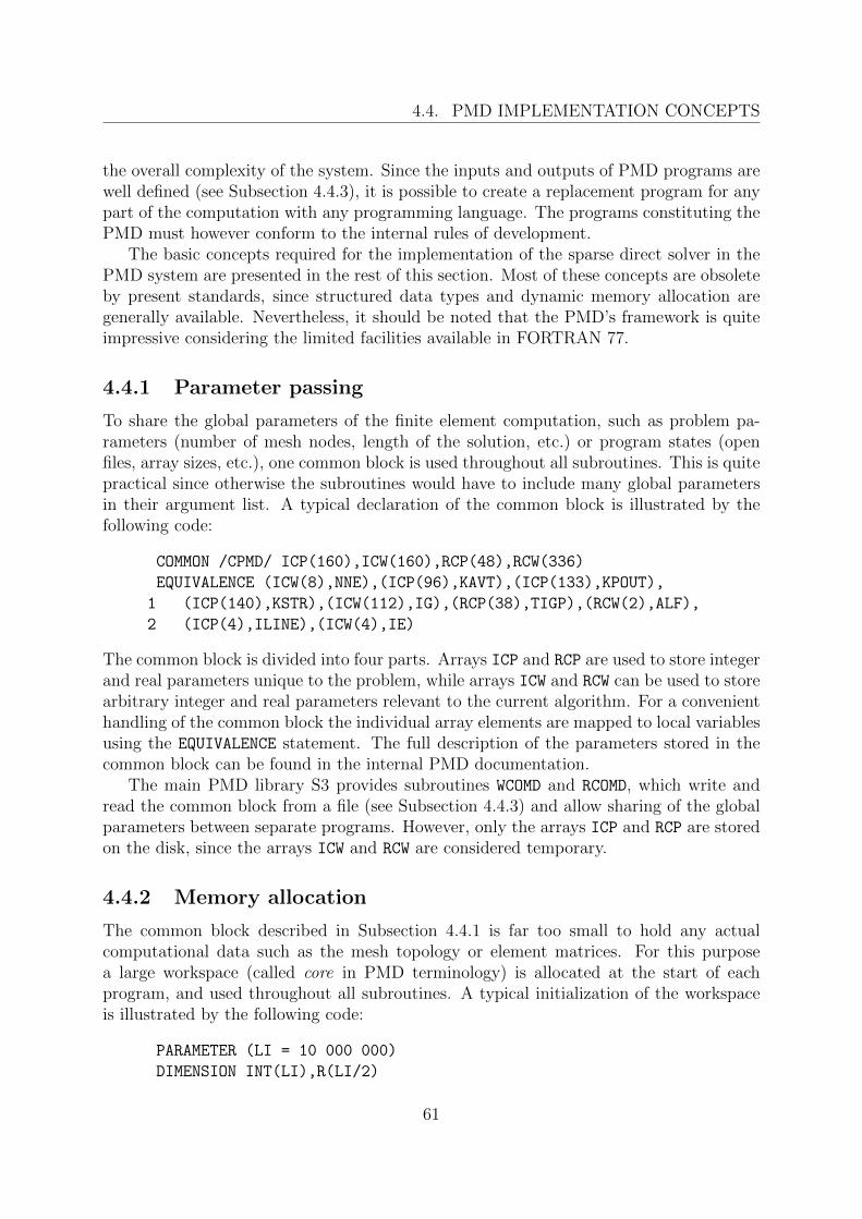
4.4. PMD IMPLEMENTATION CONCEPTS
the overall complexity of the system. Since the inputs and outputs of PMD programs arewell defined (see Subsection 4.4.3), it is possible to create a replacement program for anypart of the computation with any programming language. The programs constituting thePMD must however conform to the internal rules of development.
The basic concepts required for the implementation of the sparse direct solver in thePMD system are presented in the rest of this section. Most of these concepts are obsoleteby present standards, since structured data types and dynamic memory allocation aregenerally available. Nevertheless, it should be noted that the PMD’s framework is quiteimpressive considering the limited facilities available in FORTRAN 77.
4.4.1 Parameter passing
To share the global parameters of the finite element computation, such as problem pa-rameters (number of mesh nodes, length of the solution, etc.) or program states (openfiles, array sizes, etc.), one common block is used throughout all subroutines. This is quitepractical since otherwise the subroutines would have to include many global parametersin their argument list. A typical declaration of the common block is illustrated by thefollowing code:
COMMON /CPMD/ ICP(160),ICW(160),RCP(48),RCW(336)
EQUIVALENCE (ICW(8),NNE),(ICP(96),KAVT),(ICP(133),KPOUT),
1 (ICP(140),KSTR),(ICW(112),IG),(RCP(38),TIGP),(RCW(2),ALF),
2 (ICP(4),ILINE),(ICW(4),IE)
The common block is divided into four parts. Arrays ICP and RCP are used to store integerand real parameters unique to the problem, while arrays ICW and RCW can be used to storearbitrary integer and real parameters relevant to the current algorithm. For a convenienthandling of the common block the individual array elements are mapped to local variablesusing the EQUIVALENCE statement. The full description of the parameters stored in thecommon block can be found in the internal PMD documentation.
The main PMD library S3 provides subroutines WCOMD and RCOMD, which write andread the common block from a file (see Subsection 4.4.3) and allow sharing of the globalparameters between separate programs. However, only the arrays ICP and RCP are storedon the disk, since the arrays ICW and RCW are considered temporary.
4.4.2 Memory allocation
The common block described in Subsection 4.4.1 is far too small to hold any actualcomputational data such as the mesh topology or element matrices. For this purposea large workspace (called core in PMD terminology) is allocated at the start of eachprogram, and used throughout all subroutines. A typical initialization of the workspaceis illustrated by the following code:
PARAMETER (LI = 10 000 000)
DIMENSION INT(LI),R(LI/2)
61
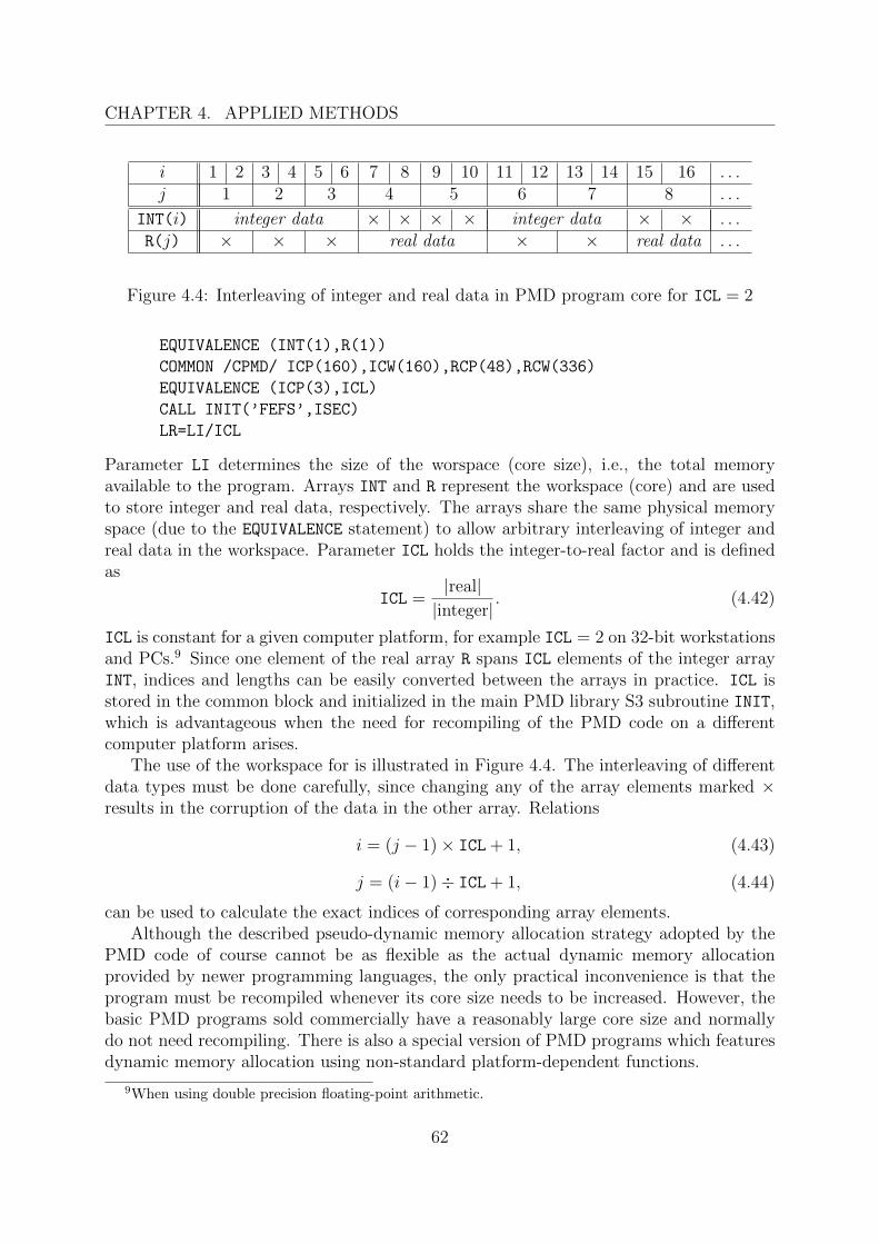
CHAPTER 4. APPLIED METHODS
i 1 2 3 4 5 6 7 8 9 10 11 12 13 14 15 16 . . .j 1 2 3 4 5 6 7 8 . . .
INT(i) integer data × × × × integer data × × . . .R(j) × × × real data × × real data . . .
Figure 4.4: Interleaving of integer and real data in PMD program core for ICL = 2
EQUIVALENCE (INT(1),R(1))
COMMON /CPMD/ ICP(160),ICW(160),RCP(48),RCW(336)
EQUIVALENCE (ICP(3),ICL)
CALL INIT(’FEFS’,ISEC)
LR=LI/ICL
Parameter LI determines the size of the worspace (core size), i.e., the total memoryavailable to the program. Arrays INT and R represent the workspace (core) and are usedto store integer and real data, respectively. The arrays share the same physical memoryspace (due to the EQUIVALENCE statement) to allow arbitrary interleaving of integer andreal data in the workspace. Parameter ICL holds the integer-to-real factor and is definedas
ICL =|real||integer|
. (4.42)
ICL is constant for a given computer platform, for example ICL = 2 on 32-bit workstationsand PCs.9 Since one element of the real array R spans ICL elements of the integer arrayINT, indices and lengths can be easily converted between the arrays in practice. ICL isstored in the common block and initialized in the main PMD library S3 subroutine INIT,which is advantageous when the need for recompiling of the PMD code on a differentcomputer platform arises.
The use of the workspace for is illustrated in Figure 4.4. The interleaving of differentdata types must be done carefully, since changing any of the array elements marked ×results in the corruption of the data in the other array. Relations
i = (j − 1)× ICL + 1, (4.43)
j = (i− 1)÷ ICL + 1, (4.44)
can be used to calculate the exact indices of corresponding array elements.Although the described pseudo-dynamic memory allocation strategy adopted by the
PMD code of course cannot be as flexible as the actual dynamic memory allocationprovided by newer programming languages, the only practical inconvenience is that theprogram must be recompiled whenever its core size needs to be increased. However, thebasic PMD programs sold commercially have a reasonably large core size and normallydo not need recompiling. There is also a special version of PMD programs which featuresdynamic memory allocation using non-standard platform-dependent functions.
9When using double precision floating-point arithmetic.
62
4.4. PMD IMPLEMENTATION CONCEPTS
4.4.3 Input and output files
To ensure the interoperability between PMD programs and facilitate their input andouput, a simple system of data files is adopted. All data files belonging to the sameproblem have the same user-chosen name name, while the extension is determined by thetype of data contained within, as is customary.
The most important are the input files (name.Ic) and the output files (name.Oc),where c is an alphanumeric character identifying the particular program or programs thatutilize the particular file. Input files are formatted and are used by the user to input allparameters and data needed by the particular program in a readable text format. Inputfiles are general-purpose, meaning that they may contain as little as a few integer andreal parameters (for example name.I4), or as much as the full description of the finiteelement mesh (for example name.I1). Output files are also formatted and are used bythe programs to output the requested results back to the user in a readable text format.Output files usually contain additional information about the program runtime, such asthe used CPU time. The full description of the PMD input and output files can be foundin [32].
Other data files are unformatted to allow efficient read and write operations, andare intended only for the internal use in PMD programs. For example, file name.CMNis used to store the common block described in Subsection 4.4.1. If the structure of aparticular data file needs to be known, for example when modifying an existing programor developing a new program, the appropriate description can be found in the internalPMD documentation.
63


Chapter 5
Results and discussion
In this chapter the theoretical results as well as the practical results of the work are pre-sented and discussed. The first section explains in detail the modifications proposed tothe matrix storage method, the ordering method, and the solution method, to enhancetheir effectiveness specifically in the case of large finite element problems. The second sec-tion describes the particular use of the abovementioned methods in a sparse direct solverdesigned for the PMD finite element system. The third section presents the numericalresults obtained with the sparse direct solver, and also includes a performance comparisonwith the existing frontal solver of the PMD system, to demonstrate the efficiency of thesparse direct solver.
Results presented in Section 5.1 have been already partially published in papers [39,40, 41, 42, 43].
5.1 Proposed algorithms
When the size of a finite element problem exceeds a certain level (say, 106 equations) theeffectiveness of the matrix storage method, the ordering method, and the solution methodbecomes highly dependent on the effectiveness of the actual algorithms. Practically, thereare only limited possibilities for the theoretical improvement of any of the methods, how-ever the underlying algorithms do present a potential for refinement. Nevertheless, theapplied methods have been thoroughly analyzed and new algorithms were devised withregard to the solution of large finite element problems. The findings are discussed in thissection.
5.1.1 Matrix storage method
The initial matrix storage method chosen for the sparse direct solver was the K3 storageformat (see Subsection 4.1.1), to facilitate an efficient in-core solution of large finite ele-ment problems. However, during the testing of the sparse direct solver, it has been foundthat the K3 storage format is severely limited on 32-bit platforms by the 2 GB memory
65
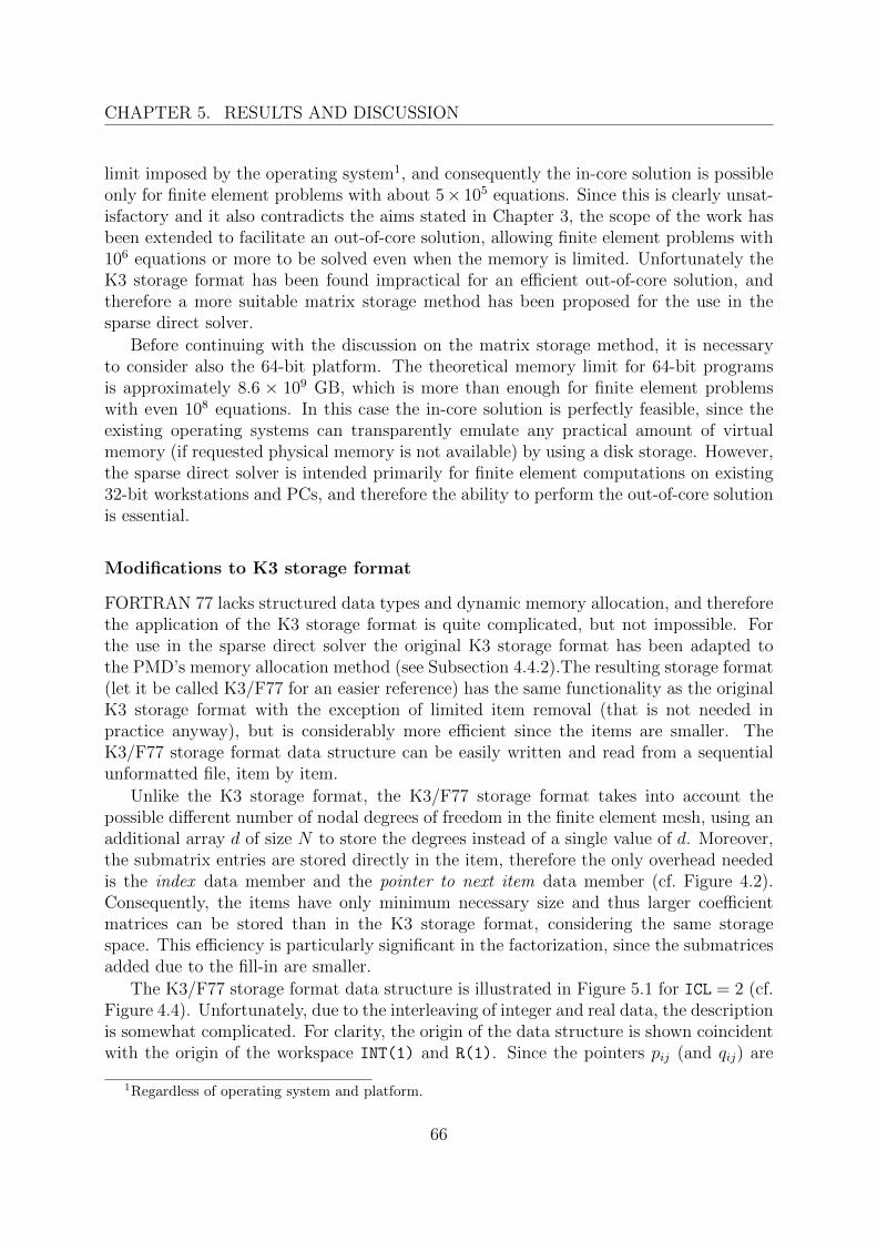
CHAPTER 5. RESULTS AND DISCUSSION
limit imposed by the operating system1, and consequently the in-core solution is possibleonly for finite element problems with about 5× 10⁵ equations. Since this is clearly unsat-isfactory and it also contradicts the aims stated in Chapter 3, the scope of the work hasbeen extended to facilitate an out-of-core solution, allowing finite element problems with106 equations or more to be solved even when the memory is limited. Unfortunately theK3 storage format has been found impractical for an efficient out-of-core solution, andtherefore a more suitable matrix storage method has been proposed for the use in thesparse direct solver.
Before continuing with the discussion on the matrix storage method, it is necessaryto consider also the 64-bit platform. The theoretical memory limit for 64-bit programsis approximately 8.6 × 109 GB, which is more than enough for finite element problemswith even 108 equations. In this case the in-core solution is perfectly feasible, since theexisting operating systems can transparently emulate any practical amount of virtualmemory (if requested physical memory is not available) by using a disk storage. However,the sparse direct solver is intended primarily for finite element computations on existing32-bit workstations and PCs, and therefore the ability to perform the out-of-core solutionis essential.
Modifications to K3 storage format
FORTRAN 77 lacks structured data types and dynamic memory allocation, and thereforethe application of the K3 storage format is quite complicated, but not impossible. Forthe use in the sparse direct solver the original K3 storage format has been adapted tothe PMD’s memory allocation method (see Subsection 4.4.2).The resulting storage format(let it be called K3/F77 for an easier reference) has the same functionality as the originalK3 storage format with the exception of limited item removal (that is not needed inpractice anyway), but is considerably more efficient since the items are smaller. TheK3/F77 storage format data structure can be easily written and read from a sequentialunformatted file, item by item.
Unlike the K3 storage format, the K3/F77 storage format takes into account thepossible different number of nodal degrees of freedom in the finite element mesh, using anadditional array d of size N to store the degrees instead of a single value of d. Moreover,the submatrix entries are stored directly in the item, therefore the only overhead neededis the index data member and the pointer to next item data member (cf. Figure 4.2).Consequently, the items have only minimum necessary size and thus larger coefficientmatrices can be stored than in the K3 storage format, considering the same storagespace. This efficiency is particularly significant in the factorization, since the submatricesadded due to the fill-in are smaller.
The K3/F77 storage format data structure is illustrated in Figure 5.1 for ICL = 2 (cf.Figure 4.4). Unfortunately, due to the interleaving of integer and real data, the descriptionis somewhat complicated. For clarity, the origin of the data structure is shown coincidentwith the origin of the workspace INT(1) and R(1). Since the pointers pij (and qij) are
1Regardless of operating system and platform.
66
5.1. PROPOSED ALGORITHMS
Pointers to first row item
u 1 2 3 . . . N − 2 N − 1 N . . .v × . . .
INT(u) p11 p22 p33 . . . pN−2,N−2 pN−1,N−1 pNN . . .R(v) × . . .
Diagonal item
u . . . pii pii + 1 pii + 2 × pii + kii − 1 . . .v . . . × qii . . . qii + lii − 1 . . .
INT(u) . . . ∗ i × . . .R(v) . . . × Aii . . .
Nondiagonal item
u . . . pij pij + 1 pij + 2 × pij + kij − 1 . . .v . . . × qij . . . qij + lij − 1 . . .
INT(u) . . . ∗ j × . . .R(v) . . . × Aij . . .
Legend:N number of nodesi nodal row index (row corresponding to node i)j nodal column index (column corresponding to node i)pij pointer to item corresponding to nodes i, jkij length of item corresponding to nodes i, jqij pointer to nodal submatrix corresponding to nodes i, jlij length of nodal submatrix corresponding to nodes i, jAij nodal submatrix corresponding to nodes i, j∗ pointer to the next item on the row, 0 if it is the last item× not applicable indices or elementsu, v workspace array element indices
Figure 5.1: K3/F77 storage format data structure
67
CHAPTER 5. RESULTS AND DISCUSSION
always relative to the origin of the data structure, it can be placed (almost) anywherein the workspace. In practice, the data structure is placed at the end of the allocatedworkspace, since it uses the whole remaining part of the workspace for the storage ofitems.
The first N array elements of the data structure are reserved for row pointers2 (pointersto the first item of the row). The items are stored as in the K3 storage format by rowsusing linked lists, beginning with the diagonal item and continuing with the nondiagonalitems sorted ascendingly by the column index. However, all items in the K3/F77 storageformat are stored dynamically, unlike the K3 storage format, where the diagonal itemsare stored separately in a static array. Another difference is that all items store the nodalcolumn index in the index data member, to simplify storage algorithms (the number ofnonzero items is not needed in practice anyway).
The initial size of the data structure is
L0 = [(N + ICL− 1)÷ ICL]× ICL, (5.1)
where ICL (integer-to-real factor, see Subsection 4.4.2) is used to align integer and realdata to the same length. All row pointers are initially zero (indicating a null value). Newitems are added to the data structure simply beginning from index L+ 1, and the storagesize L is then increased by the size of the added item, whichis
kij = (lij + h)× ICL, (5.2)
where h is the size of item overhead, defined as
h = 1÷ ICL + 1. (5.3)
In the K3/F77 storage format, the overhead is the two additional integers that are storedwith the submatrix, i.e., the index data member and the pointer to next item data member.The size of a nodal submatrix is
lij =
{di(di + 1)/2 when i = jdidj when i 6= j
, (5.4)
where di and dj are the number of degrees of freedom of node i and node j, respectively.Any item can be located only by using the integer indices (pointers), without any
additional calculations. However, after locating the required item in the data structure,the index (pointer) must be converted from the integer array INT to the real array R toaccess the submatrix entries, using equation
qij = (pij − 1)÷ ICL + h. (5.5)
The size of the K3/F77 storage format data structure is
L = |degrees|+ |row pointers|+ |items| == (N + L0 + Nnzh× ICL + Lnz × ICL)× |integer|, (5.6)
2Actual pointers are replaced with array indices in FORTRAN 77.
68
5.1. PROPOSED ALGORITHMS
where Nnz is the number of nonzero submatrices (number of items), and Lnz is the summedlength of all nonzero submatrices. Considering two practical cases ICL = 1 and ICL = 2,and separating integer and real parts, the size of the data structure is approximately
L.= (2N + 1 + 2Nnz)× |integer|+ Lnz × |real|. (5.7)
As with the K3 storage format, the data structure is created dynamically and thereforeL does not need to be known in advance.
In the out-of-core solution, submatrices of the coefficient matrix need to be written todisk and read back to the memory efficiently. One possibility for an efficient out-of-coredisk storage is to use a direct-access file with Nnz records, assign each item a number, says, and write each item to the record number s. The problem is that the item number wouldhave to be stored within the item, augmenting the overhead h substantially due to dataalignment. Considering the complicated index conversion in equation (5.5) and the needfor careful data alignment, the K3 storage format (and its modification) is impractical foran out-of-core sparse direct solver in FORTRAN 77.
Although the K3/F77 storage format is replaced in the sparse direct solver by thefollowing proposed storage format, its concept of dynamic allocation of items is reused inthe minimum degree ordering to perform symbolic assembly of the coefficient matrix andconstruct the quotient graph (see Subsection 5.1.2).
Proposed block sparse storage format
A simple and efficient matrix storage method for the out-of-core sparse direct solver isproposed in this work. It is partially based on the findings acquired from the K3/F77storage format, and partially on the compressed row storage format and the dynamicblock compressed row storage format, described in Section 2.3.2.
The proposed storage format has the following features:
• Only one-dimensional arrays are employed that are easy to understand and imple-ment in FORTRAN 77 using the PMD memory allocation strategy.
• Integer and real data are stored in separate arrays and thus no index conversionsare necessary.
• General finite element meshes with variable number of nodal degrees of freedomas well as the prescribed boundary conditions are taken into account, i.e., nodalsubmatrices can be of variable size.
• Nodal submatrices are numbered implicitly to allow an efficient out-of-core datamanipulation using direct-access file.
• The size of the data structure is the same or less than in the K3/F77 storage format.
69
CHAPTER 5. RESULTS AND DISCUSSION
The proposed storage format uses four arrays: ri, ck, pk and sl, where i = 1, . . . , N + 1(N is the number of nodes in the finite element mesh), k = 1, . . . , Nnz (Nnz is the numberof nonzero submatrices in the coefficient matrix) and l = 1, . . . , Lnz (Lnz is the sum ofthe lengths of all nonzero submatrices). Arrays r and c store row pointers and columnindices similar to the compressed row storage format, array s stores the submatrices, andarray p stores the pointers to the submatrices in array s.
Aside from the four abovementioned arrays, an important additional array d of sizeN is necessary to store the number of free nodal degrees of freedom. Since equationscorresponding to zero boundary conditions are removed from the coefficient matrix, it isefficient to store only the remaining active equations. The submatrices corresponding tonodes that have some of the degrees fixed have smaller size, and lower di results in lowerfill-in size in nodal row i. Obviously, completely fixed nodes (di = 0) are not stored inthe proposed storage format.
The size of the proposed storage format data structure is
L = |d|+ |r|+ |c|+ |p|+ |s| = (2N + 1 + 2Nnz)× |integer|+ Lnz × |real|, (5.8)
that is indeed no larger that the size of K3/F77 storage format given by equation (5.7).One difficulty is that the nonzero structure of the coefficient matrix must be known in
advance in order to create arrays r and c. However, in practice, the nonzero structure ofthe assembled coefficient matrix can be obtained from the finite element mesh topology,while the nonzero structure of the factorized matrix can be obtained from the ordering(see Subsection 5.1.2).
When the storage data structure is created, arrays r and c are initialized accordingto the nonzero structure of the matrix, and all elements in array p are initialized to 0 toindicate that the corresponding submatrix has not yet been stored in array s. The initiallength of the data in array s is Ls = 0.
In the matrix assembly, when a nodal submatrix corresponding to nodes i and j isassembled, its index k is found in cq, where q = ri, . . . , ri+1 − 1. If pk = 0 the submatrixis stored to entries st where t = Ls + 1, . . . , Ls + lij and Ls is increased by the length ofthe submatrix lij given inequation (5.4). If pk > 0 the submatrix is added to entries stwhere t = pk, . . . , pk + lij − 1.
In the matrix factorization, it is only necessary to handle the condition pk = 0, i.e., theaddition of fill-in. In this case the entries st where t = Ls + 1, . . . , Ls + lij are initializedto 0 and Ls is increased the same way as in the matrix assembly.
If there is enough memory to store all nonzero submatrices, i.e., if array s has lengthLnz, an in-core solution can be performed without difficulty.Otherwise, when the actualsize of array s is smaller than Lnz, an out-of-core solution is necessary. In the out-of-coresolution, the situation when a submatrix needs to be added to the storage but there isno more space in array s must be implemented efficiently. One possible way (althoughnot too efficient) is to write all submatrices k for which pk > 0 to disk, set pk = 0for all k, set Ls = 0, and then continue with the solution. Of course, the out-of-corefactorization algorithm must check pointer array p to ensure all submatrices required forthe actual elimination step are present in the storage array s, and load them from the
70
5.1. PROPOSED ALGORITHMS
disk if necessary. This concept can be easily extended to both the assembly algorithmand the (forward and back) substititon algorithm.
In conclusion, the proposed block sparse storage format is very efficient in both thestorage overhead (resulting in low matrix storage size) and the algorithmic overhead(resulting in quick accessibility of matrix entries). It allows the sparse direct solver toperform all necessary operations on the coefficient matrix (assembly, factorization andsubstitution) either in-core or out-of-core, depending on the amount of available memory.Efficient out-of-core data manipulation is provided by using direct-access file.
5.1.2 Ordering method
The ordering method chosen for the sparse direct solver is the approximate minimumdegree ordering algorithm (see Subsection 4.2.1), to minimize the fill-in introduced in thesparse factorization, and consequently to reduce the storage requirements and the timeneeded to obtain the solution. Although established implementations of the approximateminimum degree ordering are available, their use in a commercial sparse direct solver isprohibited,and the possibility for modifications is limited. Therefore, an original versionof the minimum degree algorithm is proposed for the use in the sparse direct solver. Thisversion is capable of selective switching of various features (supervariables, approximatedegrees, etc.) to allow the efficiency of the algorithm to be analyzed thoroughly.
Proposed minimum degree algorithm
Common implementations of the minimum degree algorithm work with the nonzero struc-ture of the matrix, i.e., directly with the matrix entries. In the application to the sparsedirect solver, it is advantageous to perform the ordering on the block nonzero structureof the matrix instead. Since the fill-in can occur only in blocks due to the block sparsestorage format, the ordering performed on matrix entries is unnecessarily expensive. Ex-ploiting of the block structure reduces the number of graph vertices and edges involvedin the minimum degree algorithm considerably. An important consequence is that the or-dering can be carried out only using the finite element mesh topology (with only integerarithmetic involved), without assembling the coefficient matrix explicitly. For large finiteelement problems the ordering on matrix blocks is significantly faster compared to theordering on matrix entries.
This almost natural improvement is surprisingly not commonly mentioned, one excep-tion being [27]. It is probably because many solvers are standalone, i.e., they are designedto work with any supplied matrix without knowing anything about the origin or the struc-ture of the matrix. Some solvers optionally allow the user to input the information aboutthe matrix structure, or use special algorithms to identify and exploit the block nonzeropattern of the matrix themselves (however, such algorithms are costly, especially for largematrices). The presented sparse direct solver is integrated into the PMD system, and istherefore capable to utilize the properties of the finite element mesh directly, without userintervention.
71
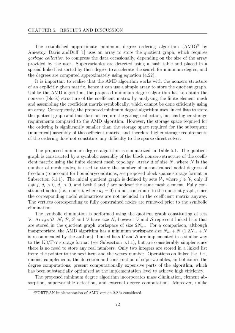
CHAPTER 5. RESULTS AND DISCUSSION
The established approximate minimum degree ordering algorithm (AMD)3 byAmestoy, Davis andDuff [1] uses an array to store the quotient graph, which requiresgarbage collection to compress the data occasionally, depending on the size of the arrayprovided by the user. Supervariables are detected using a hash table and placed in aspecial linked list sorted by their degree to accelerate the search for minimum degree, andthe degrees are computed approximately using equation (4.22).
It is important to realize that the AMD algorithm works with the nonzero structureof an explicitly given matrix, hence it can use a simple array to store the quotient graph.Unlike the AMD algorithm, the proposed minimum degree algorithm has to obtain thenonzero (block) structure of the coefficient matrix by analyzing the finite element meshand assembling the coefficient matrix symbolically, which cannot be done efficiently usingan array. Consequently, the proposed minimum degree algorithm uses linked lists to storethe quotient graph and thus does not require the garbage collection, but has higher storagerequirements compared to the AMD algorithm. However, the storage space required forthe ordering is significantly smaller than the storage space required for the subsequent(numerical) assembly of thecoefficient matrix, and therefore higher storage requirementsof the ordering does not constitute any difficulty to the sparse direct solver.
The proposed minimum degree algorithm is summarized in Table 5.1. The quotientgraph is constructed by a symbolic assembly of the block nonzero structure of the coeffi-cient matrix using the finite element mesh topology. Array d of size N , where N is thenumber of mesh nodes, is used to store the number of unconstrained nodal degrees offreedom (to account for boundaryconditions, see proposed block sparse storage format inSubsection 5.1.1). The initial quotient graph is defined by sets Vi, where j ∈ Vi only ifi 6= j, di > 0, dj > 0, and both i and j are nodesof the same mesh element. Fully con-strained nodes (i.e., nodes k where dk = 0) do not contribute to the quotient graph, sincethe corresponding nodal submatrices are not included in the coefficient matrix anyway.The vertices corresponding to fully constrained nodes are removed prior to the symbolicelimination.
The symbolic elimination is performed using the quotient graph constituting of setsV . Arrays D, N , P , S and V have size N , however V and S represent linked lists thatare stored in the quotient graph workspace of size 2Nnz. For a comparison, althoughinappropriate, the AMD algorithm has a minimum workspace size Nnz + N (1.2Nnz + Nis recommended by the authors). Linked lists V and S are implemented in a similar wayto the K3/F77 storage format (see Subsection 5.1.1), but are considerably simpler sincethere is no need to store any real numbers. Only two integers are stored in a linked listitem: the pointer to the next item and the vertex number. Operations on linked list, i.e.,unions, complements, the detection and construction of supervariables, and of course thedegree computations, present computationally expensive parts of the algorithm, whichhas been substantially optimized at the implementation level to achieve high efficiency.
The proposed minimum degree algorithm incorporates mass elimination, element ab-sorption, supervariable detection, and external degree computation. Moreover, unlike
3FORTRAN implementation of AMD version 2.2 is considered.
72
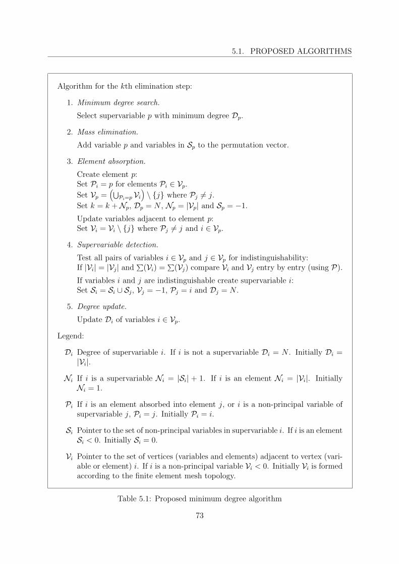
5.1. PROPOSED ALGORITHMS
Algorithm for the kth elimination step:
1. Minimum degree search.
Select supervariable p with minimum degree Dp.
2. Mass elimination.
Add variable p and variables in Sp to the permutation vector.
3. Element absorption.
Create element p:Set Pi = p for elements Pi ∈ Vp.Set Vp =
(⋃Pi=p Vi
)\ {j} where Pj 6= j.
Set k = k +Np, Dp = N , Np = |Vp| and Sp = −1.
Update variables adjacent to element p:Set Vi = Vi \ {j} where Pj 6= j and i ∈ Vp.
4. Supervariable detection.
Test all pairs of variables i ∈ Vp and j ∈ Vp for indistinguishability:If |Vi| = |Vj| and
∑(Vi) =
∑(Vj) compare Vi and Vj entry by entry (using P).
If variables i and j are indistinguishable create supervariable i:Set Si = Si ∪ Sj, Vj = −1, Pj = i and Dj = N .
5. Degree update.
Update Di of variables i ∈ Vp.
Legend:
Di Degree of supervariable i. If i is not a supervariable Di = N . Initially Di =|Vi|.
Ni If i is a supervariable Ni = |Si| + 1. If i is an element Ni = |Vi|. InitiallyNi = 1.
Pi If i is an element absorbed into element j, or i is a non-principal variable ofsupervariable j, Pi = j. Initially Pi = i.
Si Pointer to the set of non-principal variables in supervariable i. If i is an elementSi < 0. Initially Si = 0.
Vi Pointer to the set of vertices (variables and elements) adjacent to vertex (vari-able or element) i. If i is a non-principal variable Vi < 0. Initially Vi is formedaccording to the finite element mesh topology.
Table 5.1: Proposed minimum degree algorithm
73
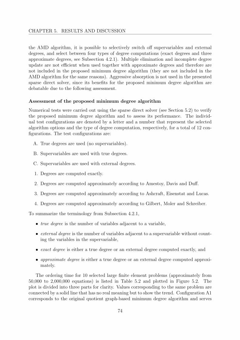
CHAPTER 5. RESULTS AND DISCUSSION
the AMD algorithm, it is possible to selectively switch off supervariables and externaldegrees, and select between four types of degree computations (exact degrees and threeapproximate degrees, see Subsection 4.2.1). Multiple elimination and incomplete degreeupdate are not efficient when used together with approximate degrees and therefore arenot included in the proposed minimum degree algorithm (they are not included in theAMD algorithm for the same reasons). Aggressive absorption is not used in the presentedsparse direct solver, since its benefits for the proposed minimum degree algorithm aredebatable due to the following assessment.
Assessment of the proposed minimum degree algorithm
Numerical tests were carried out using the sparse direct solver (see Section 5.2) to verifythe proposed minimum degree algorithm and to assess its performance. The individ-ual test configurations are denoted by a letter and a number that represent the selectedalgorithm options and the type of degree computation, respectively, for a total of 12 con-figurations. The test configurations are:
A. True degrees are used (no supervariables).
B. Supervariables are used with true degrees.
C. Supervariables are used with external degrees.
1. Degrees are computed exactly.
2. Degrees are computed approximately according to Amestoy, Davis and Duff.
3. Degrees are computed approximately according to Ashcraft, Eisenstat and Lucas.
4. Degrees are computed approximately according to Gilbert, Moler and Schreiber.
To summarize the terminology from Subsection 4.2.1,
• true degree is the number of variables adjacent to a variable,
• external degree is the number of variables adjacent to a supervariable without count-ing the variables in the supervariable,
• exact degree is either a true degree or an external degree computed exactly, and
• approximate degree is either a true degree or an external degree computed approxi-mately.
The ordering time for 10 selected large finite element problems (approximately from50,000 to 2,000,000 equations) is listed in Table 5.2 and plotted in Figure 5.2. Theplot is divided into three parts for clarity. Values corresponding to the same problem areconnected by a solid line that has no real meaning but to show the trend. Configuration A1corresponds to the original quotient graph-based minimum degree algorithm and serves
74
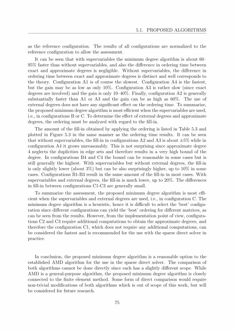
5.1. PROPOSED ALGORITHMS
as the reference configuration. The results of all configurations are normalized to thereference configuration to allow the assessment.
It can be seen that with supervariables the minimum degree algorithm is about 60–95% faster than without supervariables, and also the difference in ordering time betweenexact and approximate degrees is negligible. Without supervariables, the difference inordering time between exact and approximate degrees is distinct and well corresponds tothe theory. Configuration A1 is of course the slowest. Configuration A4 is the fastest,but the gain may be as low as only 10%. Configuration A3 is rather slow (since exactdegrees are involved) and the gain is only 10–40%. Finally, configuration A2 is generallysubstantially faster than A1 or A3 and the gain can be as high as 60%. The use ofexternal degrees does not have any significant effect on the ordering time. To summarize,the proposed minimum degree algorithm is most efficient when the supervariables are used,i.e., in configurations B or C. To determine the effect of external degrees and approximatedegrees, the ordering must be analyzed with regard to the fill-in.
The amount of the fill-in obtained by applying the ordering is listed in Table 5.3 andplotted in Figure 5.3 in the same manner as the ordering time results. It can be seenthat without supervariables, the fill-in in configurations A2 and A3 is about ±5% while inconfiguration A4 it grows unreasonably. This is not surprising since approximate degree4 neglects the duplicities in edge sets and therefore results in a very high bound of thedegree. In configurations B4 and C4 the bound can be reasonable in some cases but isstill generally the highest. With supervariables but without external degrees, the fill-inis only slightly lower (about 3%) but can be also surprisingly higher, up to 10% in somecases. Configurations B1-B3 result in the same amount of the fill-in in most cases. Withsupervariables and external degrees, the fill-in is much lower, up to 20%. The differencesin fill-in between configurations C1-C3 are generally small.
To summarize the assessment, the proposed minimum degree algorithm is most effi-cient when the supervariables and external degrees are used, i.e., in configuration C. Theminimum degree algorithm is a heuristic, hence it is difficult to select the ‘best’ configu-ration since different configurations can yield the ‘best’ ordering for different matrices, ascan be seen from the results. However, from the implementation point of view, configura-tions C2 and C3 require additional computations to obtain the approximate degrees, andtherefore the configuration C1, which does not require any additional computations, canbe considered the fastest and is recommended for the use with the sparse direct solver inpractice.
In conclusion, the proposed minimum degree algorithm is a reasonable option to theestablished AMD algorithm for the use in the sparse direct solver. The comparison ofboth algorithms cannot be done directly since each has a slightly different scope. WhileAMD is a general-purpose algorithm, the proposed minimum degree algorithm is closelyconnected to the finite element method. Some form of direct comparison would requirenon-trivial modifications of both algorithms which is out of scope of this work, but willbe considered for future research.
75
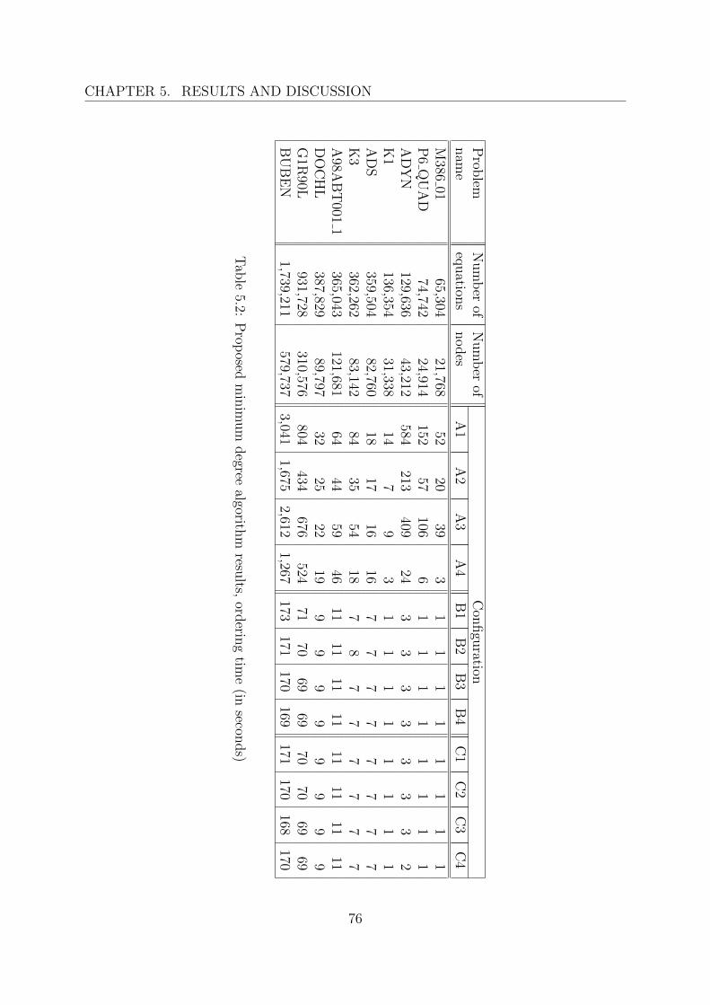
CHAPTER 5. RESULTS AND DISCUSSION
Prob
lemN
um
ber
ofN
um
ber
ofC
onfigu
rationnam
eeq
uation
snodes
A1
A2
A3
A4
B1
B2
B3
B4
C1
C2
C3
C4
M386
0165,304
21,76852
2039
31
11
11
11
1P
6Q
UA
D74,742
24,914152
57106
61
11
11
11
1A
DY
N129,636
43,212584
213409
243
33
33
33
2K
1136,354
31,33814
79
31
11
11
11
1A
DS
359,50482,760
1817
1616
77
77
77
77
K3
362,26283,142
8435
5418
78
77
77
77
A98A
BT
0011
365,043121,681
6444
5946
1111
1111
1111
1111
DO
CH
L387,829
89,79732
2522
199
99
99
99
9G
1R90L
931,728310,576
804434
676524
7170
6969
7070
6969
BU
BE
N1,739,211
579,7373,041
1,6752,612
1,267173
171170
169171
170168
170
Tab
le5.2:
Prop
osedm
inim
um
degree
algorithm
results,
orderin
gtim
e(in
seconds)
76

5.1. PROPOSED ALGORITHMS
A1
A2
A3
A4
0%10%
20%
30%
40%
50%
60%
70%
80%
90%
100%
Tru
e D
egre
es
Ordering time (relative to A1)
B1
B2
B3
B4
0%10%
20%
30%
40%
50%
60%
70%
80%
90%
100%
Alg
orith
m c
onfig
urat
ion
Sup
erva
riabl
es &
Tru
e D
egre
es
B
UB
EN
G1R
90L
DO
CH
LA
98A
BT
001_
1K
3A
DS
K1
AD
YN
P6_
QU
AD
M38
6_01
C1
C2
C3
C4
0%10%
20%
30%
40%
50%
60%
70%
80%
90%
100%
Sup
erva
riabl
es &
Ext
erna
l Deg
rees
Fig
ure
5.2:
Pro
pos
edm
inim
um
deg
ree
algo
rith
mre
sult
s,or
der
ing
tim
e
77
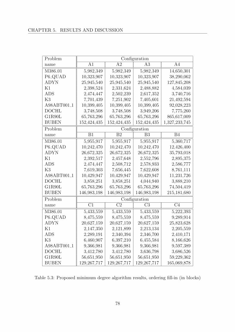
CHAPTER 5. RESULTS AND DISCUSSION
Problem Configurationname A1 A2 A3 A4
M386 01 5,982,349 5,982,349 5,982,349 14,650,301P6 QUAD 10,323,907 10,323,907 10,323,907 38,290,062ADYN 25,945,540 25,945,540 25,945,540 127,845,208K1 2,398,524 2,331,624 2,488,882 4,584,039ADS 2,474,447 2,502,239 2,617,352 3,740,716K3 7,701,439 7,251,902 7,405,601 21,492,594A98ABT001 1 10,399,405 10,399,405 10,399,405 92,028,223DOCHL 3,748,508 3,748,508 3,949,206 7,775,260G1R90L 65,763,296 65,763,296 65,763,296 865,617,009BUBEN 152,424,435 152,424,435 152,424,435 1,327,233,745
Problem Configurationname B1 B2 B3 B4
M386 01 5,955,917 5,955,917 5,955,917 5,360,717P6 QUAD 10,242,470 10,242,470 10,242,470 12,426,400ADYN 26,672,325 26,672,325 26,672,325 35,793,018K1 2,392,517 2,457,648 2,552,796 2,895,375ADS 2,474,447 2,508,712 2,578,933 2,586,777K3 7,619,303 7,656,445 7,622,608 8,761,111A98ABT001 1 10,429,947 10,429,947 10,429,947 11,231,726DOCHL 3,858,251 3,858,251 4,044,940 3,888,210G1R90L 65,763,296 65,763,296 65,763,296 74,504,419BUBEN 146,983,198 146,983,198 146,983,198 215,181,680
Problem Configurationname C1 C2 C3 C4
M386 01 5,433,559 5,433,559 5,433,559 5,222,393P6 QUAD 8,475,559 8,475,559 8,475,559 9,289,914ADYN 20,627,159 20,627,159 20,627,159 25,823,628K1 2,147,350 2,121,899 2,213,134 2,205,559ADS 2,289,191 2,340,394 2,346,700 2,410,171K3 6,460,907 6,397,210 6,455,584 8,166,626A98ABT001 1 9,366,981 9,366,981 9,366,981 9,597,389DOCHL 3,412,780 3,412,780 3,636,798 3,686,526G1R90L 56,651,950 56,651,950 56,651,950 59,229,362BUBEN 129,267,717 129,267,717 129,267,717 165,069,878
Table 5.3: Proposed minimum degree algorithm results, ordering fill-in (in blocks)
78
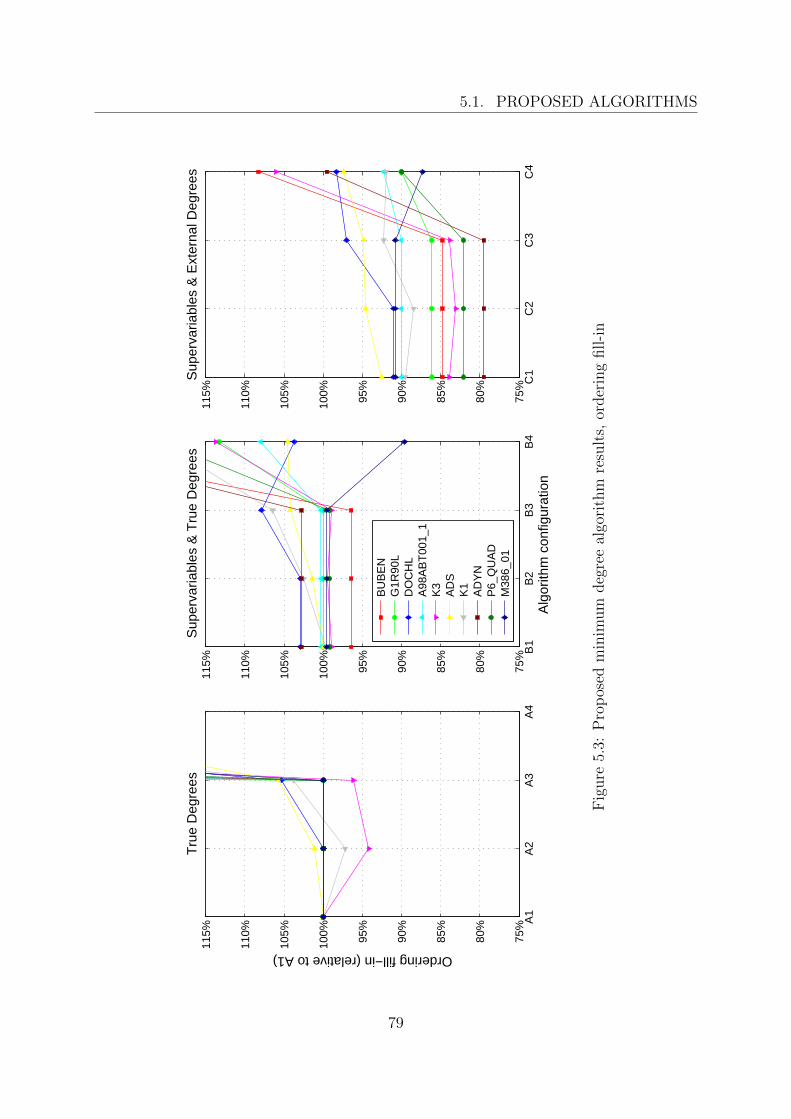
5.1. PROPOSED ALGORITHMS
A1
A2
A3
A4
75%
80%
85%
90%
95%
100%
105%
110%
115%
Tru
e D
egre
es
Ordering fill−in (relative to A1)
B1
B2
B3
B4
75%
80%
85%
90%
95%
100%
105%
110%
115%
Alg
orith
m c
onfig
urat
ion
Sup
erva
riabl
es &
Tru
e D
egre
es
BU
BE
NG
1R90
LD
OC
HL
A98
AB
T00
1_1
K3
AD
SK
1A
DY
NP
6_Q
UA
DM
386_
01
C1
C2
C3
C4
75%
80%
85%
90%
95%
100%
105%
110%
115%
Sup
erva
riabl
es &
Ext
erna
l Deg
rees
Fig
ure
5.3:
Pro
pos
edm
inim
um
deg
ree
algo
rith
mre
sult
s,or
der
ing
fill-i
n
79
CHAPTER 5. RESULTS AND DISCUSSION
5.1.3 Solution method
The solution method chosen for the sparse direct solver is the block LDLT factorization(see Subsection 4.3.1). In Subsection 5.1.1 the practical impossibility to solve large finiteelement problems in-core have been explained. Therefore, an out-of-core symmetric blocksparse factorization algorithm is proposed for the use in the sparse direct solver.
Proposed out-of-core symmetric block sparse factorization algorithm
There are four possibilities to perform the LDLT factorization. It can be carried outeither by a left-looking algorithm (using factor L) or a right-looking algorithm (usingfactor DLT), and either by rows or by columns. The number of arithmetic operationsis equivalent in all cases, therefore the most suitable algorithm can be selected based onother properties. Obviously, for an out-of-core factorization the most important questionis which part of the coefficient matrix must be present in a factorization step if thewhole coefficient matrix cannot be stored in-core. It is of course possible to design theout-of-core algorithm so that only two or three submatrices (blocks) that are involvedin the actually summed term are present in the memory at any given time, which isvery efficient in terms of the storage space but extremely inefficient in terms of the out-of-core data manipulation, since many submatrices must be read from and/or written to diskrepetitively and disk access is slow compared to memory access. A reasonable compromiseis when all submatrices involved in the computation of the actual submatrix are present inthe memory, since additional reads and writes are still required but reduced considerably.The most suitable out-of-core case, in which the efficiency of the factorization is notaffected, is when the whole active part of the coefficient matrix (active submatrix) ispresent in the memory. In any case, the out-of-core factorization algorithm checks thepresence of blocks required for the actual factorization step in the matrix storage andreads them from the disk if not present. In the case the matrix storage is full all blocksare written to disk and discarded before reading the required blocks.
The partially reduced coefficient matrix after the kth factorization step in the right-looking algorithm has the form
Ak+1|rightrow = Ak+1|rightcolumn =
d11 · · · d11lk1 d11lk+1,1 · · · d11ln1. . .
......
...dkk dkklk+1,k · · · dkklnk
dk+1,k+1 · · · dk+1,k+1ln,k+1
a(k+1)k+2,k+2 · · · a
(k+1)k+2,n
......
0 a(k+1)n,k+1 · · · a(k+1)
nn
. (5.9)
Matrix (5.9) is identical for both the row-wise approach (common Gaussian elimination)and the column-wise approach (uncommon, impractical). Rows 1, . . . , k already containfactor entries dii and lji that are however not used in any of the subsequent factorization
80
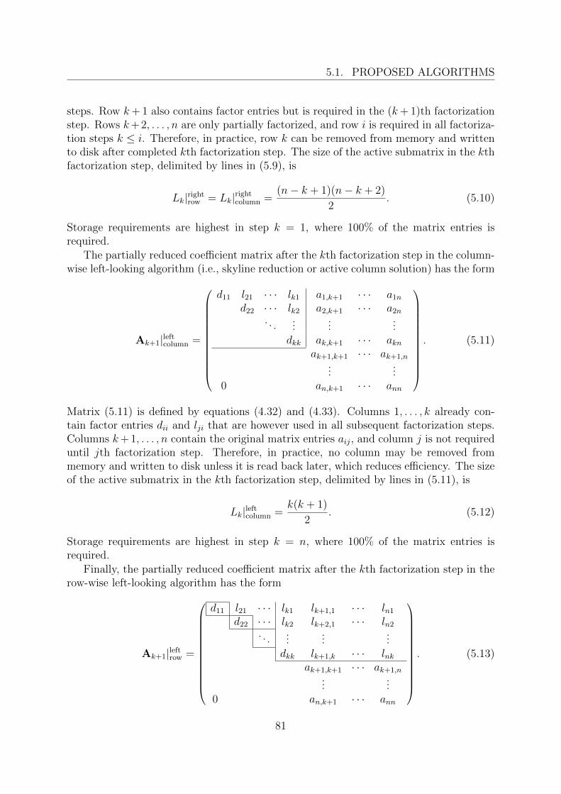
5.1. PROPOSED ALGORITHMS
steps. Row k + 1 also contains factor entries but is required in the (k + 1)th factorizationstep. Rows k+ 2, . . . , n are only partially factorized, and row i is required in all factoriza-tion steps k ≤ i. Therefore, in practice, row k can be removed from memory and writtento disk after completed kth factorization step. The size of the active submatrix in the kthfactorization step, delimited by lines in (5.9), is
Lk|rightrow = Lk|rightcolumn =(n− k + 1)(n− k + 2)
2. (5.10)
Storage requirements are highest in step k = 1, where 100% of the matrix entries isrequired.
The partially reduced coefficient matrix after the kth factorization step in the column-wise left-looking algorithm (i.e., skyline reduction or active column solution) has the form
Ak+1|leftcolumn =
d11 l21 · · · lk1 a1,k+1 · · · a1nd22 · · · lk2 a2,k+1 · · · a2n
. . ....
......
dkk ak,k+1 · · · aknak+1,k+1 · · · ak+1,n
......
0 an,k+1 · · · ann
. (5.11)
Matrix (5.11) is defined by equations (4.32) and (4.33). Columns 1, . . . , k already con-tain factor entries dii and lji that are however used in all subsequent factorization steps.Columns k+ 1, . . . , n contain the original matrix entries aij, and column j is not requireduntil jth factorization step. Therefore, in practice, no column may be removed frommemory and written to disk unless it is read back later, which reduces efficiency. The sizeof the active submatrix in the kth factorization step, delimited by lines in (5.11), is
Lk|leftcolumn =k(k + 1)
2. (5.12)
Storage requirements are highest in step k = n, where 100% of the matrix entries isrequired.
Finally, the partially reduced coefficient matrix after the kth factorization step in therow-wise left-looking algorithm has the form
Ak+1|leftrow =
d11 l21 · · · lk1 lk+1,1 · · · ln1d22 · · · lk2 lk+2,1 · · · ln2
. . ....
......
dkk lk+1,k · · · lnkak+1,k+1 · · · ak+1,n
......
0 an,k+1 · · · ann
. (5.13)
81
CHAPTER 5. RESULTS AND DISCUSSION
Matrix (5.13) is also defined by equations (4.32) and (4.33). Columns 1, . . . , k alreadycontain factor entries dii and lji, however entries lji are not used in any of the subsequentfactorization steps. Rows k + 1, . . . , n contain the original matrix entries aij, and row iis not required until ith factorization step. The submatrix with entry indices i = 1, . . . , kand j = k + 1, . . . , n also contains factor entries but columns j = p, . . . , n are requireduntil pth factorization step is completed.
Therefore, in practice, column k can be removed from memory (except for the diagonalentry) and written to disk after completed kth factorization step. Moreover, rows k +1, . . . , n need not to be present in memory until they are needed. The size of the activesubmatrix in the kth factorization step (including diagonal entries), delimited by linesin (5.13), is
Lk|leftrow = k(n− k + 2)− 1. (5.14)
Storage requirements are highest in step k = n/2, where only about 50% of the matrixentries is required.
In conclusion, the most efficient algorithm for an out-of-core factorization is the left-looking algorithm performed by rows, which is surprisingly not commonly mentioned.Presented conclusions can be easily extended to a block sparse coefficient matrix, in whichcase the storage requirements will be substantially lower due tosparsity. The minimumrequired storage size for factorization (i.e., the maximum size of the active submatrix)can be obtained from the symbolic elimination (using minimum degree ordering).
5.2 Solver implementation
Sparse direct solver presented in this work is based on methods and algorithms describedin Chapter 4 and, in particular, Section 5.1. The sparse direct solver (program FESD) isimplemented according to the requirements of the PMD system, described in Section 4.4,and is designed to seamlessly replace the existing PMD’s frontal solver (program FEFS).
In short, the sparse direct solver reads the mesh topology and element matrices (pre-processed by other PMD programs), solves the associated linear equation system, andwrites displacements and reaction forces (postprocessed by other PMD programs to cal-culate stresses, strains, etc.). Sparse direct solver’s input file, output file and intermediatedata files are documented in Appendix B. The intermediate data files used by the sparsedirect solver are different from the frontal solver, therefore, both solvers can coexist inthe same directory (provided the user is aware that files name.I4, name.O4 and IDSOL
are shared between the two solvers). Consequently, the coefficient matrix factorized bythe sparse direct solver cannot be used by the frontal solver and vice versa. To facilitateprogram restarts and allow the computation of additional load cases (right-hand sides), anew parameter KFES was added to the PMD common to store sparse direct solver’s status.
The presented sparse direct solver is divided logically into four distinct phases (order-ing, assembly, factorization and solution) which are described in the following sections.The source code of the sparse direct solver is documented in Appendix C.
82
5.2. SOLVER IMPLEMENTATION
5.2.1 Ordering phase
The ordering phase is perhaps the most elaborate part of the program. It comprises ofthe following steps:
1. INET, NNET, NNDF and IFIXV are read from file IDP.
2. MBD, NPIV, NVAR, LEMTX and LSMTX are calculated using INET, NNET, NNDF and IFIXV.
3. A quotient graph is created using INET and NNET.Simultaneously, NBLK1 and SBUF1 are calculated using MBD.
4. IPNOD is calculated using the minimum degree ordering on the quotient graph. Op-tionally, the (reverse) Cuthill-McKee preordering is applied.Simultaneously, MRP and MCI are calculated and written to file IDEQI.Simultaneously, NBLK2 and SBUF2 are calculated using MBD.
5. IPSOL is calculated using NNDF, MBD and IPNOD.
6. NPIV, NVAR, NBLK1, NBLK2, SBUF1, SBUF2, LSMTX, LROW, LEMTX, KMET, IPNOD, IPSOLand MBD are written to file IDEQC to facilitate solver restarts.
7. MRP and MCI are read from file IDEQI, permuted using IPNOD, and written back tofile IDEQI.
Note that the column indices written to file IDEQI in step 4 are not permuted sincethe full permutation vector IPNOD is not known until the ordering is complete. Therefore,the indices are permuted and file IDEQI is rewritten in step 7 prior to the assembly phase.
The ordering is performed using the minimum degree algorithm proposed in Subsec-tion 5.1.2, optionally coupled with the (reverse) Cuthill-McKee preordering. The outputof the ordering phase is the nonzero block structure of the coefficient matrix in the fac-torization. Consequently, appropriate storage structures can be prepared for both theassembly and the factorization phases. The implemented minimum degree ordering algo-rithm is highly optimized, particularly regarding the operations on edge sets (adding andremoving elements, joining sets, etc.).
5.2.2 Assembly phase
The assembly phase is relatively simple and comprises of the following steps:
1. Element stiffness matrix is read from file IDELM and partitioned into nodal subma-trices using INET, NNET, NNDF and IPSOL.
2. Nodal submatrices are assembled into the coefficient matrix using IPNOD, MRP, MCI,MBP and BUF.
3. Steps 1 and 2 are repeated for all elements NELEM.
83
CHAPTER 5. RESULTS AND DISCUSSION
The coefficient matrix is assembled using the block sparse storage format proposed inSubsection 5.1.1, where N ≡ NPIV, Nnz ≡ NBLK2, Lnz ≡ SBUF1, d ≡ MBP, r ≡ MRP, c ≡MCI, p ≡ MBP and s ≡ BUF. Entries corresponding to constrained degrees of freedom (zeroboundary conditions) are excluded from nodal submatrices (corresponding submatricesare therefore smaller). Nodal submatrices corresponding to fully constrained nodes arenot included in the coefficient matrix, since they have zero size. Thus, the output of theassembly phase is the assembled coefficient matrix excluding the boundary conditions.
5.2.3 Factorization phase
The factorization phase comprises of the following steps:
1. The coefficient matrix is factorized using MRP, MCI, MBP, MBD and BUF.
2. BUF is written to file IDEQR.
The factorization is performed using the block sparse factorization algorithm proposedin Subsection 5.1.3. The output of the factorization phase is the factorized coefficientmatrix. The implemented block sparse factorization algorithm is highly optimized, par-ticularly regarding the arithmetic operations performed on blocks.
After this phase is successfully finished it is possible to restart the solver with addi-tional right-hand sides using the factorized coefficient matrix (without the need to factorizeit again).
5.2.4 Solution phase
The solution phase comprises of the following steps:
1. RHS is read from file IDRHS and permuted using IPSOL.
2. Displacements are solved for all load cases NASV by forward and back substitutionusing RHS, MRP, MCI, MBP, MBD and BUF.
3. Solved displacements are permuted back using IPSOL.
4. Reaction forces are solved for all load cases NASV by assembling the appropriateequations directly from file IDELM using INET, NNET, NNDF, IPSOL and the displace-ments.
5. The displacements and the reaction forces are written to file IDSOL.
The output of the solution phase are displacement vectors and reaction force vectorsfor all load cases (right-hand sides).
84
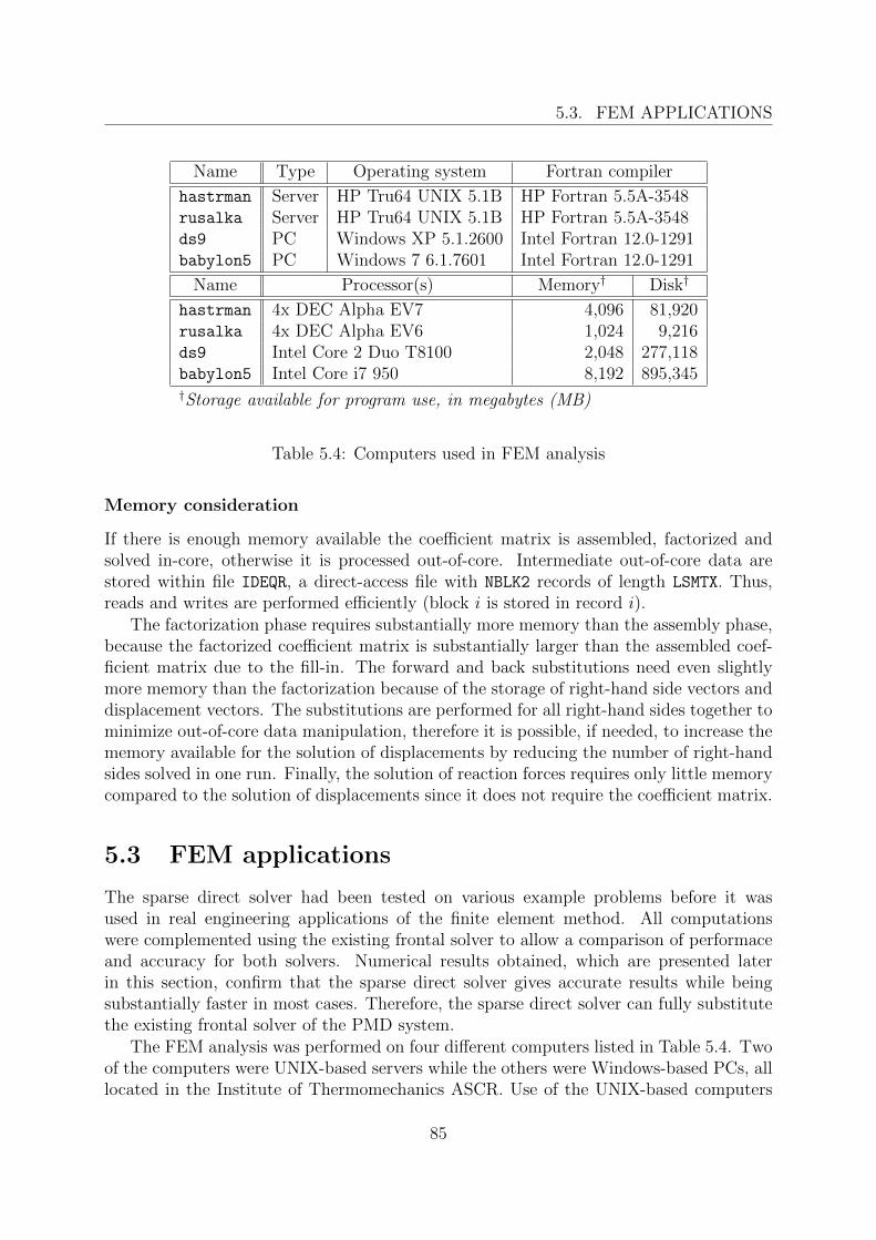
5.3. FEM APPLICATIONS
Name Type Operating system Fortran compiler
hastrman Server HP Tru64 UNIX 5.1B HP Fortran 5.5A-3548rusalka Server HP Tru64 UNIX 5.1B HP Fortran 5.5A-3548ds9 PC Windows XP 5.1.2600 Intel Fortran 12.0-1291babylon5 PC Windows 7 6.1.7601 Intel Fortran 12.0-1291
Name Processor(s) Memory† Disk†
hastrman 4x DEC Alpha EV7 4,096 81,920rusalka 4x DEC Alpha EV6 1,024 9,216ds9 Intel Core 2 Duo T8100 2,048 277,118babylon5 Intel Core i7 950 8,192 895,345†Storage available for program use, in megabytes (MB)
Table 5.4: Computers used in FEM analysis
Memory consideration
If there is enough memory available the coefficient matrix is assembled, factorized andsolved in-core, otherwise it is processed out-of-core. Intermediate out-of-core data arestored within file IDEQR, a direct-access file with NBLK2 records of length LSMTX. Thus,reads and writes are performed efficiently (block i is stored in record i).
The factorization phase requires substantially more memory than the assembly phase,because the factorized coefficient matrix is substantially larger than the assembled coef-ficient matrix due to the fill-in. The forward and back substitutions need even slightlymore memory than the factorization because of the storage of right-hand side vectors anddisplacement vectors. The substitutions are performed for all right-hand sides together tominimize out-of-core data manipulation, therefore it is possible, if needed, to increase thememory available for the solution of displacements by reducing the number of right-handsides solved in one run. Finally, the solution of reaction forces requires only little memorycompared to the solution of displacements since it does not require the coefficient matrix.
5.3 FEM applications
The sparse direct solver had been tested on various example problems before it wasused in real engineering applications of the finite element method. All computationswere complemented using the existing frontal solver to allow a comparison of performaceand accuracy for both solvers. Numerical results obtained, which are presented laterin this section, confirm that the sparse direct solver gives accurate results while beingsubstantially faster in most cases. Therefore, the sparse direct solver can fully substitutethe existing frontal solver of the PMD system.
The FEM analysis was performed on four different computers listed in Table 5.4. Twoof the computers were UNIX-based servers while the others were Windows-based PCs, alllocated in the Institute of Thermomechanics ASCR. Use of the UNIX-based computers
85
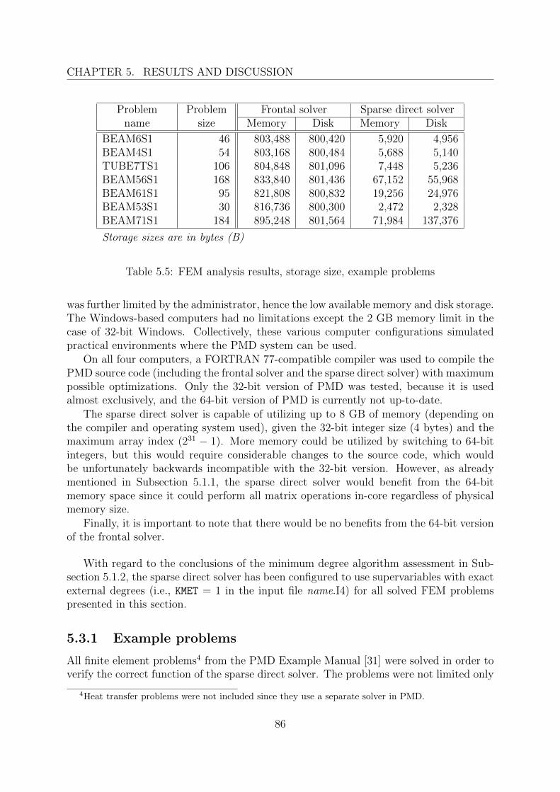
CHAPTER 5. RESULTS AND DISCUSSION
Problem Problem Frontal solver Sparse direct solvername size Memory Disk Memory Disk
BEAM6S1 46 803,488 800,420 5,920 4,956BEAM4S1 54 803,168 800,484 5,688 5,140TUBE7TS1 106 804,848 801,096 7,448 5,236BEAM56S1 168 833,840 801,436 67,152 55,968BEAM61S1 95 821,808 800,832 19,256 24,976BEAM53S1 30 816,736 800,300 2,472 2,328BEAM71S1 184 895,248 801,564 71,984 137,376
Storage sizes are in bytes (B)
Table 5.5: FEM analysis results, storage size, example problems
was further limited by the administrator, hence the low available memory and disk storage.The Windows-based computers had no limitations except the 2 GB memory limit in thecase of 32-bit Windows. Collectively, these various computer configurations simulatedpractical environments where the PMD system can be used.
On all four computers, a FORTRAN 77-compatible compiler was used to compile thePMD source code (including the frontal solver and the sparse direct solver) with maximumpossible optimizations. Only the 32-bit version of PMD was tested, because it is usedalmost exclusively, and the 64-bit version of PMD is currently not up-to-date.
The sparse direct solver is capable of utilizing up to 8 GB of memory (depending onthe compiler and operating system used), given the 32-bit integer size (4 bytes) and themaximum array index (231 − 1). More memory could be utilized by switching to 64-bitintegers, but this would require considerable changes to the source code, which wouldbe unfortunately backwards incompatible with the 32-bit version. However, as alreadymentioned in Subsection 5.1.1, the sparse direct solver would benefit from the 64-bitmemory space since it could perform all matrix operations in-core regardless of physicalmemory size.
Finally, it is important to note that there would be no benefits from the 64-bit versionof the frontal solver.
With regard to the conclusions of the minimum degree algorithm assessment in Sub-section 5.1.2, the sparse direct solver has been configured to use supervariables with exactexternal degrees (i.e., KMET = 1 in the input file name.I4) for all solved FEM problemspresented in this section.
5.3.1 Example problems
All finite element problems4 from the PMD Example Manual [31] were solved in order toverify the correct function of the sparse direct solver. The problems were not limited only
4Heat transfer problems were not included since they use a separate solver in PMD.
86
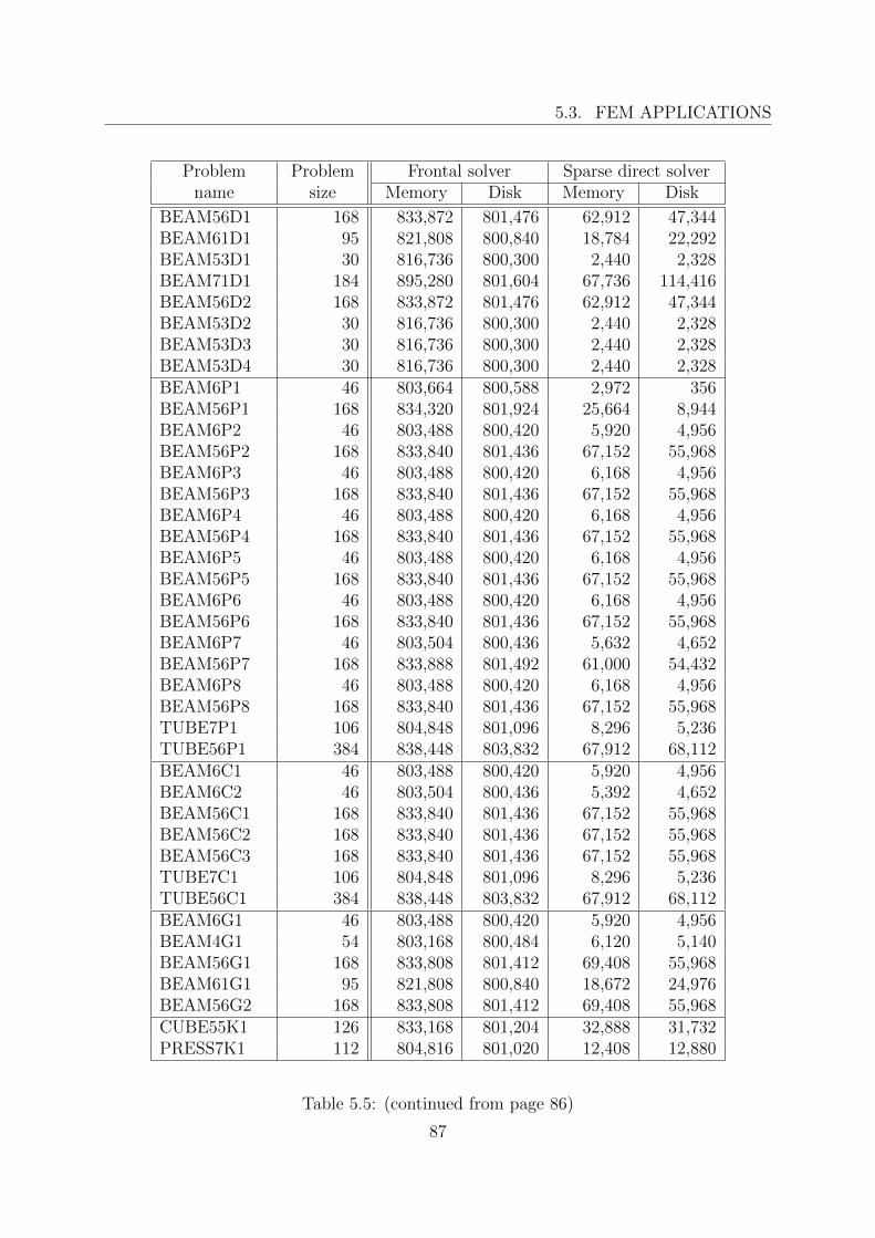
5.3. FEM APPLICATIONS
Problem Problem Frontal solver Sparse direct solvername size Memory Disk Memory Disk
BEAM56D1 168 833,872 801,476 62,912 47,344BEAM61D1 95 821,808 800,840 18,784 22,292BEAM53D1 30 816,736 800,300 2,440 2,328BEAM71D1 184 895,280 801,604 67,736 114,416BEAM56D2 168 833,872 801,476 62,912 47,344BEAM53D2 30 816,736 800,300 2,440 2,328BEAM53D3 30 816,736 800,300 2,440 2,328BEAM53D4 30 816,736 800,300 2,440 2,328BEAM6P1 46 803,664 800,588 2,972 356BEAM56P1 168 834,320 801,924 25,664 8,944BEAM6P2 46 803,488 800,420 5,920 4,956BEAM56P2 168 833,840 801,436 67,152 55,968BEAM6P3 46 803,488 800,420 6,168 4,956BEAM56P3 168 833,840 801,436 67,152 55,968BEAM6P4 46 803,488 800,420 6,168 4,956BEAM56P4 168 833,840 801,436 67,152 55,968BEAM6P5 46 803,488 800,420 6,168 4,956BEAM56P5 168 833,840 801,436 67,152 55,968BEAM6P6 46 803,488 800,420 6,168 4,956BEAM56P6 168 833,840 801,436 67,152 55,968BEAM6P7 46 803,504 800,436 5,632 4,652BEAM56P7 168 833,888 801,492 61,000 54,432BEAM6P8 46 803,488 800,420 6,168 4,956BEAM56P8 168 833,840 801,436 67,152 55,968TUBE7P1 106 804,848 801,096 8,296 5,236TUBE56P1 384 838,448 803,832 67,912 68,112BEAM6C1 46 803,488 800,420 5,920 4,956BEAM6C2 46 803,504 800,436 5,392 4,652BEAM56C1 168 833,840 801,436 67,152 55,968BEAM56C2 168 833,840 801,436 67,152 55,968BEAM56C3 168 833,840 801,436 67,152 55,968TUBE7C1 106 804,848 801,096 8,296 5,236TUBE56C1 384 838,448 803,832 67,912 68,112BEAM6G1 46 803,488 800,420 5,920 4,956BEAM4G1 54 803,168 800,484 6,120 5,140BEAM56G1 168 833,808 801,412 69,408 55,968BEAM61G1 95 821,808 800,840 18,672 24,976BEAM56G2 168 833,808 801,412 69,408 55,968CUBE55K1 126 833,168 801,204 32,888 31,732PRESS7K1 112 804,816 801,020 12,408 12,880
Table 5.5: (continued from page 86)
87
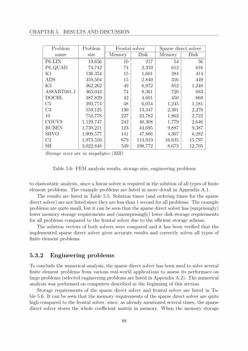
CHAPTER 5. RESULTS AND DISCUSSION
Problem Problem Frontal solver Sparse direct solvername size Memory Disk Memory Disk
P6 LIN 19,656 10 217 54 56P6 QUAD 74,742 74 2,359 612 616K1 136,354 15 1,601 284 414ADS 359,504 15 2,840 316 449K3 362,262 49 6,972 852 1,248A98ABT001 1 365,043 74 8,361 720 683DOCHL 387,829 42 4,601 450 668C5 393,774 48 6,054 1,245 1,181C3 559,125 130 13,347 2,391 2,27010 752,778 227 23,782 1,862 2,722COUV9 1,129,747 242 40,308 1,779 2,646BUBEN 1,739,211 123 44,695 9,887 9,387SHVO 1,909,577 141 47,866 4,307 6,282C2 1,973,550 679 113,919 16,635 15,797SH 3,022,848 549 198,772 8,673 12,705
Storage sizes are in megabytes (MB)
Table 5.6: FEM analysis results, storage size, engineering problems
to elastostatic analysis, since a linear solver is required in the solution of all types of finiteelement problems. The example problems are listed in more detail in Appendix A.1.
The results are listed in Table 5.5. Solution times (and ordering times for the sparsedirect solver) are not listed since they are less than 1 second for all problems. The exampleproblems are quite small, but it can be seen that the sparse direct solver has (surprisingly)lower memory storage requirements and (unsurprisingly) lower disk storage requirementsfor all problems compared to the frontal solver due to the efficient storage scheme.
The solution vectors of both solvers were compared and it has been verified that theimplemented sparse direct solver gives accurate results and correctly solves all types offinite element problems.
5.3.2 Engineering problems
To conclude the numerical analysis, the sparse direct solver has been used to solve severalfinite element problems from various real-world applications to assess its performace onlarge problems (selected engineering problems are listed in Appendix A.2). The numericalanalysis was performed on computers described in the beginning of this section.
Storage requirements of the sparse direct solver and frontal solver are listed in Ta-ble 5.6. It can be seen that the memory requirements of the sparse direct solver are quitehigh compared to the frontal solver, since, as already mentioned several times, the sparsedirect solver stores the whole coefficient matrix in memory. When the memory storage
88
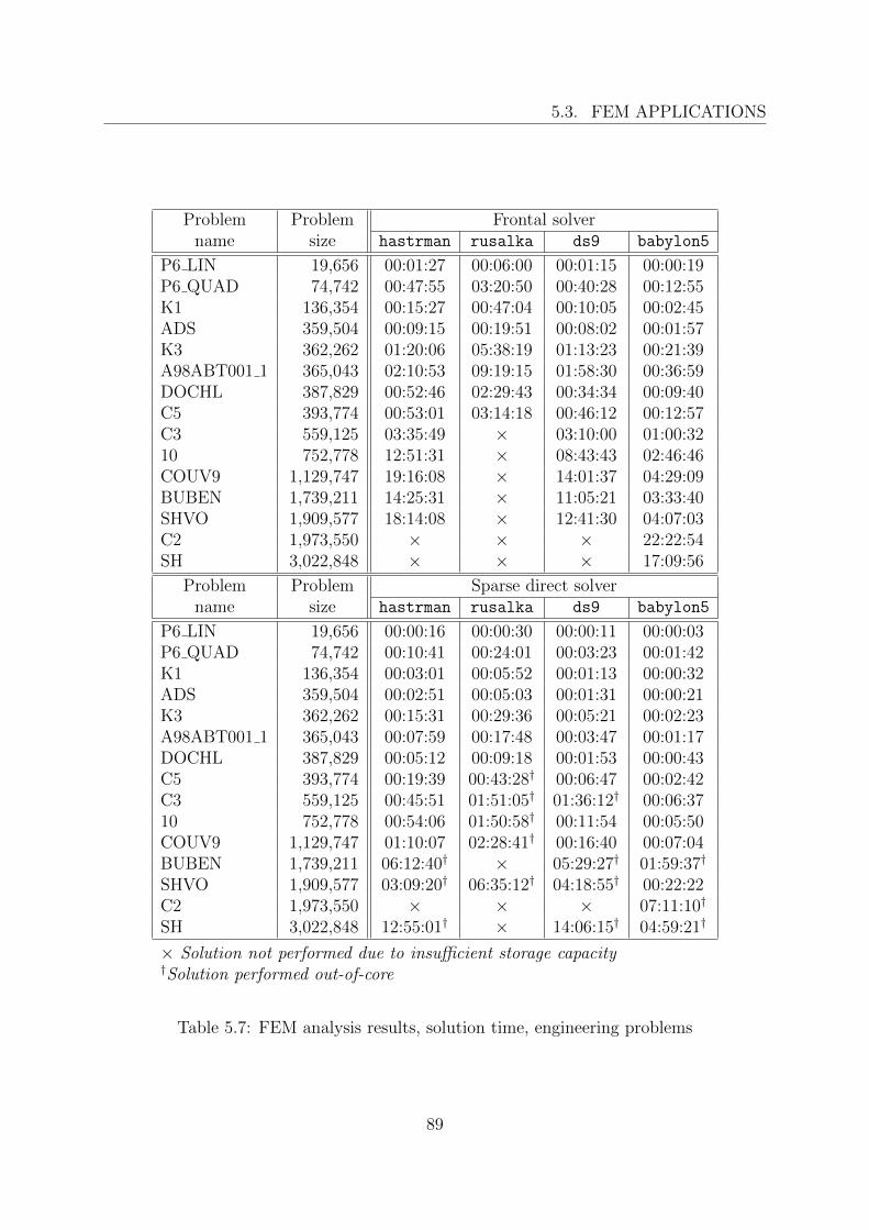
5.3. FEM APPLICATIONS
Problem Problem Frontal solvername size hastrman rusalka ds9 babylon5
P6 LIN 19,656 00:01:27 00:06:00 00:01:15 00:00:19P6 QUAD 74,742 00:47:55 03:20:50 00:40:28 00:12:55K1 136,354 00:15:27 00:47:04 00:10:05 00:02:45ADS 359,504 00:09:15 00:19:51 00:08:02 00:01:57K3 362,262 01:20:06 05:38:19 01:13:23 00:21:39A98ABT001 1 365,043 02:10:53 09:19:15 01:58:30 00:36:59DOCHL 387,829 00:52:46 02:29:43 00:34:34 00:09:40C5 393,774 00:53:01 03:14:18 00:46:12 00:12:57C3 559,125 03:35:49 × 03:10:00 01:00:3210 752,778 12:51:31 × 08:43:43 02:46:46COUV9 1,129,747 19:16:08 × 14:01:37 04:29:09BUBEN 1,739,211 14:25:31 × 11:05:21 03:33:40SHVO 1,909,577 18:14:08 × 12:41:30 04:07:03C2 1,973,550 × × × 22:22:54SH 3,022,848 × × × 17:09:56
Problem Problem Sparse direct solvername size hastrman rusalka ds9 babylon5
P6 LIN 19,656 00:00:16 00:00:30 00:00:11 00:00:03P6 QUAD 74,742 00:10:41 00:24:01 00:03:23 00:01:42K1 136,354 00:03:01 00:05:52 00:01:13 00:00:32ADS 359,504 00:02:51 00:05:03 00:01:31 00:00:21K3 362,262 00:15:31 00:29:36 00:05:21 00:02:23A98ABT001 1 365,043 00:07:59 00:17:48 00:03:47 00:01:17DOCHL 387,829 00:05:12 00:09:18 00:01:53 00:00:43C5 393,774 00:19:39 00:43:28† 00:06:47 00:02:42C3 559,125 00:45:51 01:51:05† 01:36:12† 00:06:3710 752,778 00:54:06 01:50:58† 00:11:54 00:05:50COUV9 1,129,747 01:10:07 02:28:41† 00:16:40 00:07:04BUBEN 1,739,211 06:12:40† × 05:29:27† 01:59:37†
SHVO 1,909,577 03:09:20† 06:35:12† 04:18:55† 00:22:22C2 1,973,550 × × × 07:11:10†
SH 3,022,848 12:55:01† × 14:06:15† 04:59:21†
× Solution not performed due to insufficient storage capacity†Solution performed out-of-core
Table 5.7: FEM analysis results, solution time, engineering problems
89
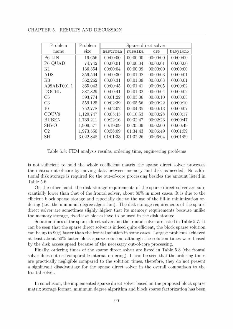
CHAPTER 5. RESULTS AND DISCUSSION
Problem Problem Sparse direct solvername size hastrman rusalka ds9 babylon5
P6 LIN 19,656 00:00:00 00:00:00 00:00:00 00:00:00P6 QUAD 74,742 00:00:01 00:00:04 00:00:01 00:00:00K1 136,354 00:00:04 00:00:09 00:00:00 00:00:00ADS 359,504 00:00:30 00:01:08 00:00:03 00:00:01K3 362,262 00:00:31 00:01:09 00:00:03 00:00:01A98ABT001 1 365,043 00:00:45 00:01:41 00:00:05 00:00:02DOCHL 387,829 00:00:41 00:01:32 00:00:04 00:00:02C5 393,774 00:01:22 00:03:06 00:00:10 00:00:05C3 559,125 00:02:39 00:05:56 00:00:22 00:00:1010 752,778 00:02:02 00:04:35 00:00:13 00:00:07COUV9 1,129,747 00:05:45 00:10:53 00:00:28 00:00:17BUBEN 1,739,211 00:22:16 00:32:47 00:02:23 00:00:47SHVO 1,909,577 00:19:09 00:35:09 00:02:00 00:00:49C2 1,973,550 00:58:09 01:34:43 00:06:49 00:01:59SH 3,022,848 01:01:33 01:32:26 00:06:04 00:01:59
Table 5.8: FEM analysis results, ordering time, engineering problems
is not sufficient to hold the whole coefficient matrix the sparse direct solver processesthe matrix out-of-core by moving data between memory and disk as needed. No addi-tional disk storage is required for the out-of-core processing besides the amount listed inTable 5.6.
On the other hand, the disk storage requirements of the sparse direct solver are sub-stantially lower than that of the frontal solver, about 80% in most cases. It is due to theefficient block sparse storage and especially due to the use of the fill-in minimization or-dering (i.e., the minimum degree algorithm). The disk storage requirements of the sparsedirect solver are sometimes slighly higher that its memory requirements because unlikethe memory storage, fixed-size blocks have to be used in the disk storage.
Solution times of the sparse direct solver and the frontal solver are listed in Table 5.7. Itcan be seen that the sparse direct solver is indeed quite efficient, the block sparse solutioncan be up to 90% faster than the frontal solution in some cases. Largest problems achievedat least about 50% faster block sparse solution, although the solution times were biasedby the disk access speed because of the necessary out-of-core processing.
Finally, ordering times of the sparse direct solver are listed in Table 5.8 (the frontalsolver does not use comparable internal ordering). It can be seen that the ordering timesare practically negligible compared to the solution times, therefore, they do not presenta significant disadvantage for the sparse direct solver in the overall comparison to thefrontal solver.
In conclusion, the implemented sparse direct solver based on the proposed block sparsematrix storage format, minimum degree algorithm and block sparse factorization has been
90

5.3. FEM APPLICATIONS
confirmed to be an efficient and adequate complement to the existing frontal solver of thePMD system. It has high memory requirements, but in practice, this is not a difficulty forpresent computers and operating systems, and the savings in time and disk space requiredfor the solution can be up to 80% or even more. The sparse direct solver is a suitableoption especially in cases of very large problems where the frontal solver starts to haveunreasonable requirements on disk storage due to large frontwidth. However, it should benoted that there are some large problems where the frontal solution is faster, particularlywhen the frontwidth is small. As already mentioned, the minimum degree algorithm isnot guaranteed to give the best ordering for any arbitrary problem, since it is after allonly a heuristic.
91

Chapter 6
Conclusions
An efficient sparse direct solver for finite element analysis of very large problems in con-tinuum mechanics was designed. As a starting point, today’s numerical methods, whichplayed the central role in direct solution approaches, were critically analyzed and on thebasis of this, new algorithms were proposed. In the next step, the sparse direct solver wasimplemented, thouroughly tested and employed in practical applications to have provenitself in real-world engineering problems. The contribution of the work presented in thisthesis was thus both of theroretical and practical nature.
The theoretical contribution lies primarily in the proposed efficient algorithms for thestorage, ordering, and solution of large sparse linear systems. Although the appropriatemathematical methods have been around for some time, their application to sparse linearsystems with 106 equations or more becomes problematic even on contemporary com-puters, and therefore it requires special consideration and careful approach. The overallquality of the implementation of involved algorithms has a substantial impact on the so-lution time and storage size and may result in unfeasibility of the solution if inappropriatenumerical procedures were applied.
The original matrix storage method selected for the sparse direct solver was the promis-ing K3 storage format, which was, however, found unsuitable for the intended applicationduring the course of the work. Therefore, it was replaced by an efficient custom storageformat that was based on a combination of several storage schemes including the K3storage format. The proposed matrix storage format exploits sparsity and block struc-ture resulting from the finite element method to achieve minimum storage requirements,while using simple arrays that can be easily implemented in any relevant programminglanguage. Moreover, the proposed storage format allows for an out-of-core implementa-tion of the matrix assembly, factorization and resolution, which are the primary matrixoperations performed by the sparse direct solver. An out-of-core solver of course involvesmuch more complicated algorithms than an in-core solver, and it should be emphasizedthat the implemented possibility for an out-of-core solution is crucial for the practicalusability of the sparse direct solver for large finite element problems.
The minimum degree algorithm, which is one of the most commonly used orderingmethods due to its relative directness and efficiency, was implemented in a different waythan in most established codes. It was tailored to the finite element method by perform-
93
CHAPTER 6. CONCLUSIONS
ing symbolic assembly and elimination on the block nonzero structure of the coefficientmatrix, which turned out to be significantly more efficient than analyzing the nonzerostructure of the matrix entries. The linked-list based quotient graph used in the proposedminimum degree algorithm was highly optimized to allow the operations on the edgesets to be carried out in an efficient manner. The proposed minimum degree algorithmemploys all features found in the established implementations, such as supervariables, el-ement absorption, external degrees, and approximate degrees used in the state-of-the-artapproximate minimum degree algorithm (AMD). For research purposes and fine-tuningof the minimum degree algorithm, several features were set optional by outletting themto the solver’s input file. Subsection 5.1.2 presents a comprehensive assessment of theperformance of the proposed minimum degree algorithm that was used to choose the besttype of degree computation for the practical applications of the sparse direct solver. Theordering times achieved by the sparse direct solver on large problems demonstrated theeffectiveness and usability of the proposed minimum degree algorithm.
The chosen solution method (LDLT factorization) is also well known but its commonapplication is not overly well suited to large systems because of its high demands on thestorage space. To minimize the memory requirements of the factorization, it was proposedin Subsection 5.1.3 to employ a rather non-traditional left-looking algorithm performedon rows instead of on columns as was standard in skyline solvers. This reduced the size ofthe active submatrix that had to be present in the memory (core) during the factorizationsignificantly and, therefore, made the out-of-core solution more feasible since much lessout-of-core data manipulation was needed. Moreover, the solution algorithm made useof the proposed block sparse matrix storage format in order to reduce the number offloating-point operations during the factorization and resolution to minimum by skippingsubmatrix multiplications where any of the factors was zero.
On practical part, a sparse direct solver code compatible with the PMD finite el-ement system was made, based on the aforementioned algorithms. The implementedFORTRAN 77 code has been integrated into the PMD system, and now presents a fullyfeatured linear solver capable of efficient solving of large problems. The sparse direct solverwas designed to perform the three primary matrix operations (assembly, factorization andresolution) all fully in-core but, in addition, to automatically use out-of-core algorithmswhenever available memory is limited. This allowed very large finite element problems tohave been solved. One should note that by implementing this complex out-of-core sparsedirect solver, the initial requirements on the solver were significantly surpassed.
Numerical results obtained by the sparse direct solver were carefully analyzed andcompared to the existing frontal solver of the PMD system and, therefore, the correct andaccurate operation of the new solver was verified. Finally, numerical tests were carried outon several large real-world engineering problems using the finite element method. Theirresults, presented in Subsection 5.3.2, clearly demonstrated the abundant effectiveness ofthe sparse direct solver compared to the existing frontal solver.
In conclusion, while the aims of this thesis were accomplished, further workshould be directed towards the integration of the new solution procedures into the dynamicand non-linear branch of the PMD system to fully exploit the effectiveness of this fastlinear solver. Another interesting line of development is the implementation of the sparse
94
direct solver on 64-bit platforms, where the benefits of the sparse factorization can beutilized fully due to virtually unlimited available memory.
95

Bibliography
[1] Amestoy P. R., Davis T. A. and Duff I. S. (2004). Algorithm 837: AMD, an ap-proximate minimum degree ordering algorithm. ACM Transactions on MathematicalSoftware, 30, 3, pp. 381–388.
[2] Amestoy P. R., Davis T. A. and Duff I. S. (1996). An approximate minimum de-gree ordering algorithm. SIAM Journal on Matrix Analysis and Applications, 17, 4,pp. 886–905.
[3] Bai Z., Demmel J., Dongarra J., Ruhe A. and van der Vorst H., editors (2000).Templates for the solution of algebraic eigenvalue problems: A practical guide. SIAM,Philadelphia.
[4] Barnard S. T., Pothen A. and Simon H. D. (1993). A spectral algorithm for enve-lope reduction of sparse matrices. Proceedings of the 1993 ACM/IEEE conference onSupercomputing, pp. 493–502.
[5] Bathe K. J. (1996). Finite element procedures. Prentice-Hall, Upper Saddle River,NJ.
[6] Blackford L. S., Demmel J., Dongarra J., Duff I. S., Hammarling S., Henry G.,Heroux H., Kaufman L., Lumsdaine A., Petitet A., Pozo R., Remington K., andWhaley R. C. (2002). An updated set of basic linear algebra subprograms (BLAS).ACM Transactions on Mathematical Software, 28, 2, pp. 135–151.
[7] Botsch M., Bommes D. and Kobbelt L. (2005). Efficient linear system solvers for meshprocessing. In: Martin R. R., Bez H. E. and Sabin M. A., editors. IMA Conferenceon the Mathematics of Surfaces, 3604, pp. 62–83. Springer, Berlin.
[8] Cavers I.A. (1989). Using deficiency measure for tiebreaking the minimum degreealgorithm. Technical Report TR-89-02. University of British Columbia, Vancouver,BC.
[9] Cuthill E. and McKee J. (1969). Reducing the bandwidth of sparse symmetric ma-trices. Proceedings of the 1969 24th national conference, pp. 157–172.
[10] Davis T. A. (2009). Summary of available software for sparse direct methods. http://www.cise.ufl.edu/research/sparse/codes/. Retrieved on April 1, 2009.
97
BIBLIOGRAPHY
[11] Diestel R. (2000). Graph theory, 2nd edition. Springer, New York.
[12] Duff I. S. and Scott J. A. (2005). Towards an automatic ordering for a symmet-ric sparse direct solver. Technical Report RAL-TR-2006-001. Rutherford AppletonLaboratory, Oxon.
[13] Duff I. S. (1998). Matrix methods. Technical Report RAL-TR-1998-076. RutherfordAppleton Laboratory, Oxon.
[14] Duff I. S. (1998). Direct methods. Technical Report RAL-TR-1998-054. RutherfordAppleton Laboratory, Oxon.
[15] Duff I. S. (1997). Sparse numerical linear algebra: direct methods and preconditioning.Technical Report RAL-TR-96-047. Rutherford Appleton Laboratory, Oxon.
[16] Duff I. S. and Reid J. K. (1983). The multifrontal solution of indefinite sparse symmet-ric linear systems. ACM Transactions on Mathematical Software, 9, 3, pp. 302–325.
[17] Duff I. S. and Reid J. K. (1982). MA27—A set of Fortran subroutines for solv-ing sparse symmetric sets of linear equations. Technical Report AERE R10533. HerMajesty’s Stationery Office, London.
[18] George A. and Liu J. W. H. (1981). Computer solution of large sparse positive definitesystems. Prentice-Hall, Englewood Cliffs, NJ.
[19] George A. and Liu J. W. H. (1989). The evolution of the minimum degree orderingalgorithm. SIAM Review, 31, 1, pp. 1–19.
[20] George A. and Liu J. W. H. (1980). A fast implementation of the minimum degreealgorithm using quotient graphs. ACM Transactions on Mathematical Software, 6,3, pp. 337–358.
[21] George A. (1973). Nested dissection of a regular finite element mesh. SIAM Journalon Numerical Analysis, 10, 2, pp. 345–363.
[22] Gilbert J. R., Moler C. and Schreiber R. (1992). Sparse matrices in MATLAB: designand implementation. SIAM Journal on Matrix Analysis and Applications, 13, 1,pp. 333-356.
[23] Gould N. I. M., Scott J. A. and Hu Y. (2007). A numerical evaluation of sparse directsolvers for the solution of large sparse symmetric linear systems of equations. ACMTransactions on Mathematical Software, 33, 2.
[24] Irons B. M. (1970). A frontal solution program for finite-element analysis. Interna-tional Journal for Numerical Methods in Engineering, 2, 1, pp. 5–32.
[25] Karypis G. and Kumar V. (1998). A fast and high quality multilevel scheme for parti-tioning irregular graphs. SIAM Journal on Scientific Computing, 20, 1, pp. 359–392.
98
BIBLIOGRAPHY
[26] Khaira M. S., Miller G. L. and Sheffler T. J. (1992). Nested Dissection: A survey andcomparison of various nested dissection algorithms. Technical Report CSD. CarnegieMellon University, Pittsburgh, PA.
[27] Kruis J. (2006). Domain decomposition methods for distributed computing. Saxe-Coburg, Glasgow.
[28] Liu J. W. H. (1985). Modification of the minimum-degree algorithm by multipleelimination. ACM Transactions on Mathematical Software, 11, 2, pp. 141–153.
[29] Markowitz H. M. (1957). The elimination form of the inverse and its application tolinear programming. Management Science, 3, 3, pp. 255–269.
[30] Okrouhlık M., editor (2008). Numerical methods in computational mechanics. Insti-tute of Thermomechanics ASCR, Prague.
[31] Plesek J. and Gabriel D. (2000). PMD Example Manual. Institute of Thermomechan-ics ASCR, Prague.
[32] PMD Reference Guide. VAMET Ltd., Prague.
[33] PMD User Guide. VAMET Ltd., Prague.
[34] Rose D. J. (1970). Symmetric elimination on sparse positive definite systems andthe potential flow network problem. Doctoral Thesis. Harvard University, Cambridge,MA.
[35] Tinney W. F. and Walker J. W. (1967). Direct solutions of sparse network equa-tions by optimally ordered triangular factorization. Proceedings of the IEEE, 55, 11,pp. 1801–1809.
[36] Ueberhuber C. W. (1994). Numerical computation. Springer, Berlin.
[37] Vondracek R. (2008). Use of a sparse direct solver in engineering applications ofthe finite element method. Doctoral Thesis. Czech Technical University in Prague,Prague.
[38] Vondrak V. (2000). Description of the K3 sparse matrix storage system. TechnicalReport, unpublished. Technical University in Ostrava, Ostrava.
Author’s publications
[39] Parık P. and Plesek J. (2009). Assessments of the implementation of the minimumdegree ordering algorithms. Pollack Periodica, International Journal for Engineeringand Information Sciences, 4, 3, pp. 121–128.
99
BIBLIOGRAPHY
[40] Parık P. (2009). Performance tests of the minimum degree ordering algorithm. En-gineering Mechanics 2009, pp. 929–935.
[41] Parık P. (2008). Implementation of a sparse direct solver for large linear systems.Vypocty konstrukcı metodou konecnych prvku 2008, pp. 98–101.
[42] Parık P. (2007). Sparse direct solver with fill-in optimization. Engineering Mechanics2007.
[43] Parık P. (2005). Numericka implementace linearnıho resice na bazi algoritmu AMD.Summer Workshop of Applied Mechanics 2005, pp. 75–84.
100
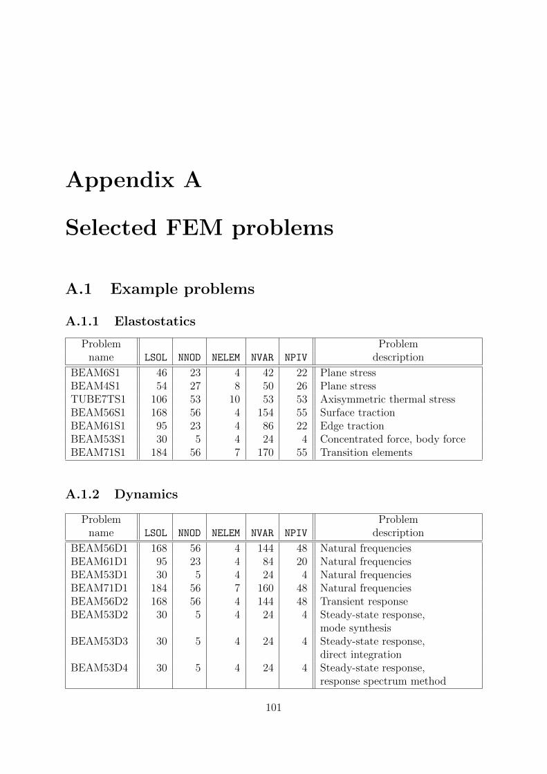
Appendix A
Selected FEM problems
A.1 Example problems
A.1.1 Elastostatics
Problem Problemname LSOL NNOD NELEM NVAR NPIV description
BEAM6S1 46 23 4 42 22 Plane stressBEAM4S1 54 27 8 50 26 Plane stressTUBE7TS1 106 53 10 53 53 Axisymmetric thermal stressBEAM56S1 168 56 4 154 55 Surface tractionBEAM61S1 95 23 4 86 22 Edge tractionBEAM53S1 30 5 4 24 4 Concentrated force, body forceBEAM71S1 184 56 7 170 55 Transition elements
A.1.2 Dynamics
Problem Problemname LSOL NNOD NELEM NVAR NPIV description
BEAM56D1 168 56 4 144 48 Natural frequenciesBEAM61D1 95 23 4 84 20 Natural frequenciesBEAM53D1 30 5 4 24 4 Natural frequenciesBEAM71D1 184 56 7 160 48 Natural frequenciesBEAM56D2 168 56 4 144 48 Transient responseBEAM53D2 30 5 4 24 4 Steady-state response,
mode synthesisBEAM53D3 30 5 4 24 4 Steady-state response,
direct integrationBEAM53D4 30 5 4 24 4 Steady-state response,
response spectrum method
101
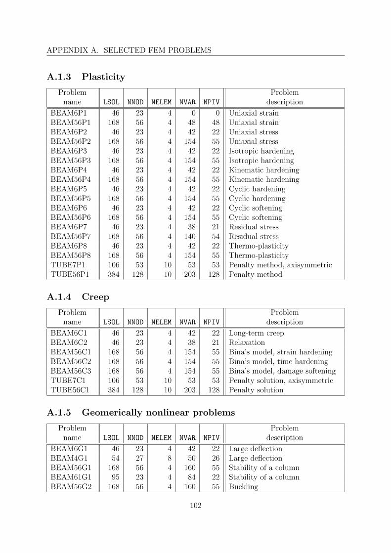
APPENDIX A. SELECTED FEM PROBLEMS
A.1.3 Plasticity
Problem Problemname LSOL NNOD NELEM NVAR NPIV description
BEAM6P1 46 23 4 0 0 Uniaxial strainBEAM56P1 168 56 4 48 48 Uniaxial strainBEAM6P2 46 23 4 42 22 Uniaxial stressBEAM56P2 168 56 4 154 55 Uniaxial stressBEAM6P3 46 23 4 42 22 Isotropic hardeningBEAM56P3 168 56 4 154 55 Isotropic hardeningBEAM6P4 46 23 4 42 22 Kinematic hardeningBEAM56P4 168 56 4 154 55 Kinematic hardeningBEAM6P5 46 23 4 42 22 Cyclic hardeningBEAM56P5 168 56 4 154 55 Cyclic hardeningBEAM6P6 46 23 4 42 22 Cyclic softeningBEAM56P6 168 56 4 154 55 Cyclic softeningBEAM6P7 46 23 4 38 21 Residual stressBEAM56P7 168 56 4 140 54 Residual stressBEAM6P8 46 23 4 42 22 Thermo-plasticityBEAM56P8 168 56 4 154 55 Thermo-plasticityTUBE7P1 106 53 10 53 53 Penalty method, axisymmetricTUBE56P1 384 128 10 203 128 Penalty method
A.1.4 Creep
Problem Problemname LSOL NNOD NELEM NVAR NPIV description
BEAM6C1 46 23 4 42 22 Long-term creepBEAM6C2 46 23 4 38 21 RelaxationBEAM56C1 168 56 4 154 55 Bina’s model, strain hardeningBEAM56C2 168 56 4 154 55 Bina’s model, time hardeningBEAM56C3 168 56 4 154 55 Bina’s model, damage softeningTUBE7C1 106 53 10 53 53 Penalty solution, axisymmetricTUBE56C1 384 128 10 203 128 Penalty solution
A.1.5 Geomerically nonlinear problems
Problem Problemname LSOL NNOD NELEM NVAR NPIV description
BEAM6G1 46 23 4 42 22 Large deflectionBEAM4G1 54 27 8 50 26 Large deflectionBEAM56G1 168 56 4 160 55 Stability of a columnBEAM61G1 95 23 4 84 22 Stability of a columnBEAM56G2 168 56 4 160 55 Buckling
102
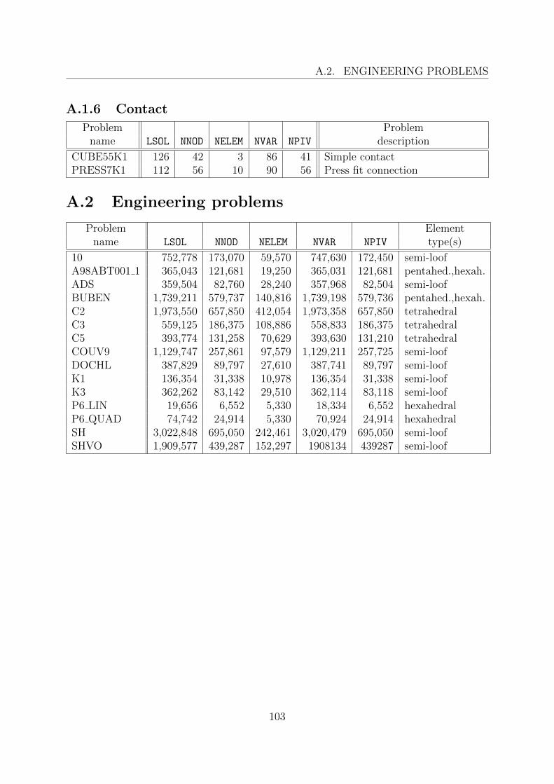
A.2. ENGINEERING PROBLEMS
A.1.6 Contact
Problem Problemname LSOL NNOD NELEM NVAR NPIV description
CUBE55K1 126 42 3 86 41 Simple contactPRESS7K1 112 56 10 90 56 Press fit connection
A.2 Engineering problems
Problem Elementname LSOL NNOD NELEM NVAR NPIV type(s)
10 752,778 173,070 59,570 747,630 172,450 semi-loofA98ABT001 1 365,043 121,681 19,250 365,031 121,681 pentahed.,hexah.ADS 359,504 82,760 28,240 357,968 82,504 semi-loofBUBEN 1,739,211 579,737 140,816 1,739,198 579,736 pentahed.,hexah.C2 1,973,550 657,850 412,054 1,973,358 657,850 tetrahedralC3 559,125 186,375 108,886 558,833 186,375 tetrahedralC5 393,774 131,258 70,629 393,630 131,210 tetrahedralCOUV9 1,129,747 257,861 97,579 1,129,211 257,725 semi-loofDOCHL 387,829 89,797 27,610 387,741 89,797 semi-loofK1 136,354 31,338 10,978 136,354 31,338 semi-loofK3 362,262 83,142 29,510 362,114 83,118 semi-loofP6 LIN 19,656 6,552 5,330 18,334 6,552 hexahedralP6 QUAD 74,742 24,914 5,330 70,924 24,914 hexahedralSH 3,022,848 695,050 242,461 3,020,479 695,050 semi-loofSHVO 1,909,577 439,287 152,297 1908134 439287 semi-loof
103
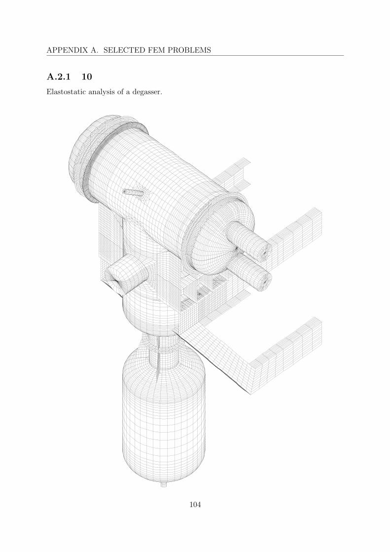
APPENDIX A. SELECTED FEM PROBLEMS
A.2.1 10
Elastostatic analysis of a degasser.
104
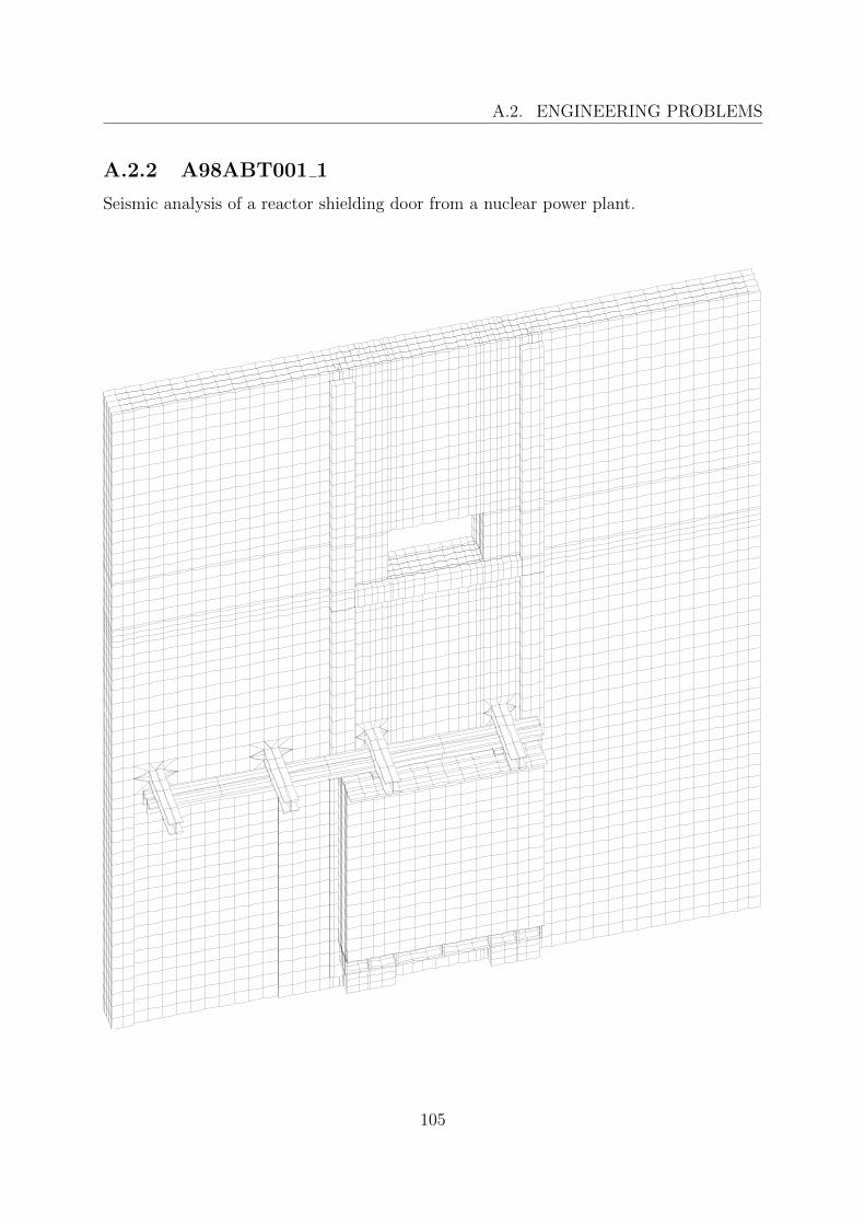
A.2. ENGINEERING PROBLEMS
A.2.2 A98ABT001 1
Seismic analysis of a reactor shielding door from a nuclear power plant.
105
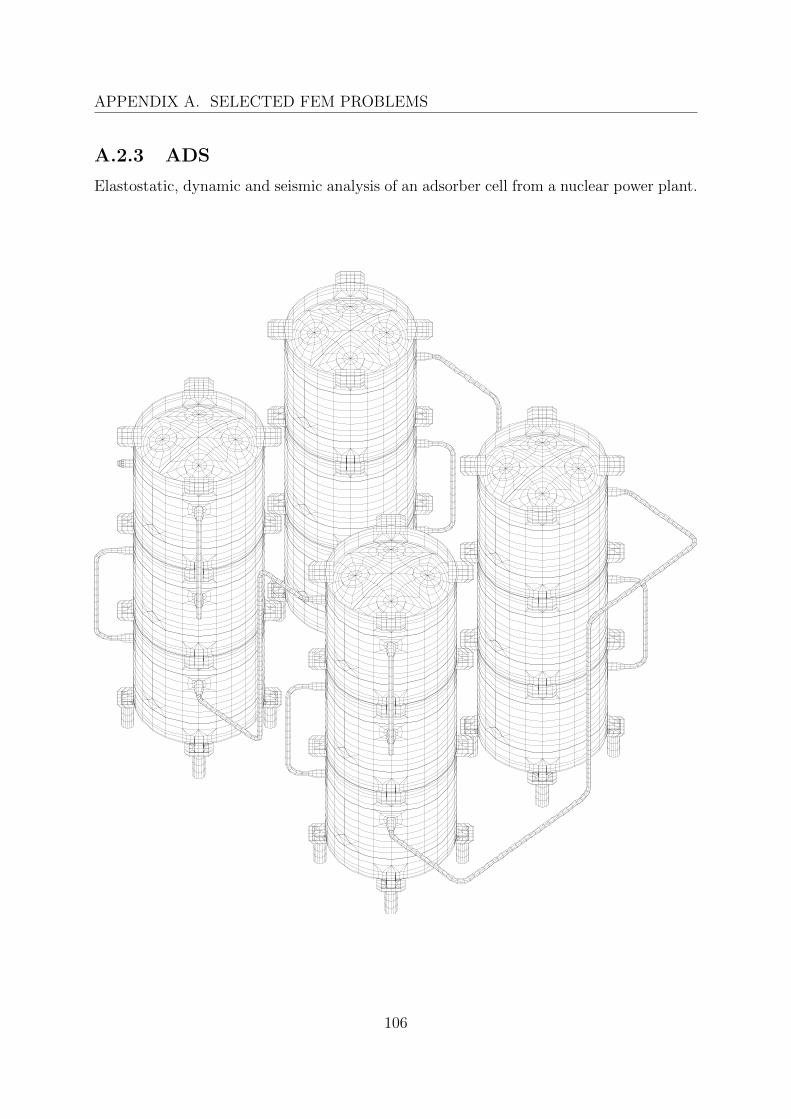
APPENDIX A. SELECTED FEM PROBLEMS
A.2.3 ADS
Elastostatic, dynamic and seismic analysis of an adsorber cell from a nuclear power plant.
106
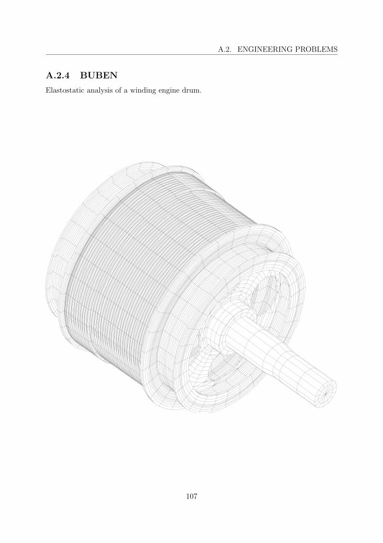
A.2. ENGINEERING PROBLEMS
A.2.4 BUBEN
Elastostatic analysis of a winding engine drum.
107
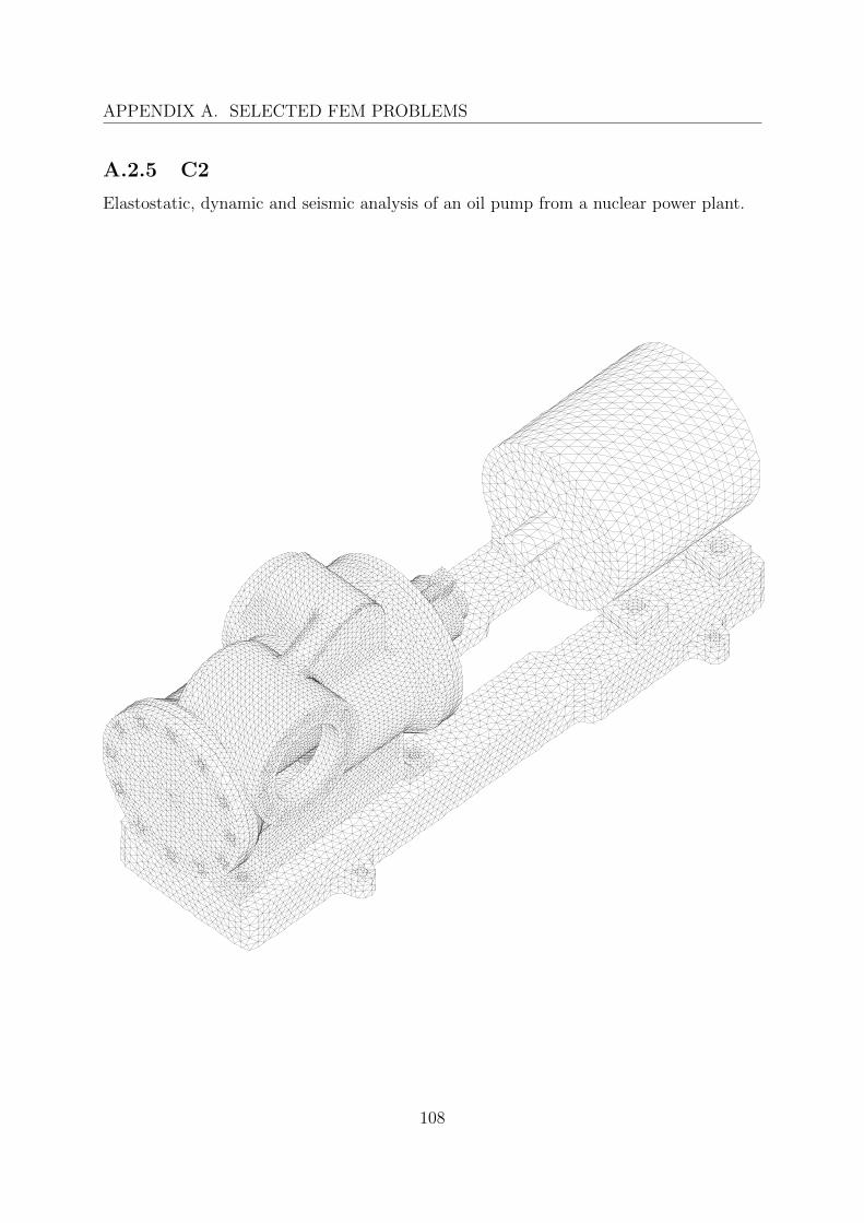
APPENDIX A. SELECTED FEM PROBLEMS
A.2.5 C2
Elastostatic, dynamic and seismic analysis of an oil pump from a nuclear power plant.
108
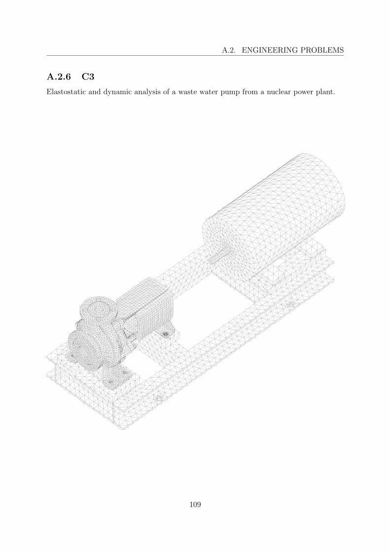
A.2. ENGINEERING PROBLEMS
A.2.6 C3
Elastostatic and dynamic analysis of a waste water pump from a nuclear power plant.
109
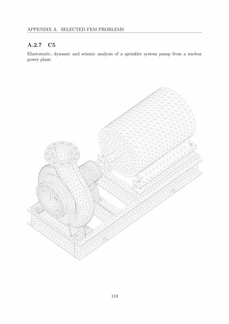
APPENDIX A. SELECTED FEM PROBLEMS
A.2.7 C5
Elastostatic, dynamic and seismic analysis of a sprinkler system pump from a nuclearpower plant.
110
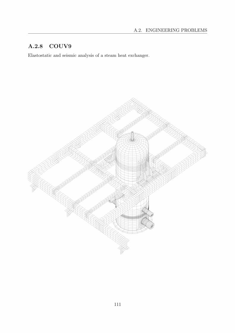
A.2. ENGINEERING PROBLEMS
A.2.8 COUV9
Elastostatic and seismic analysis of a steam heat exchanger.
111
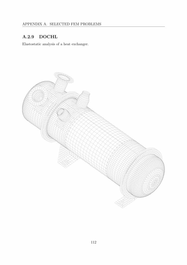
APPENDIX A. SELECTED FEM PROBLEMS
A.2.9 DOCHL
Elastostatic analysis of a heat exchanger.
112
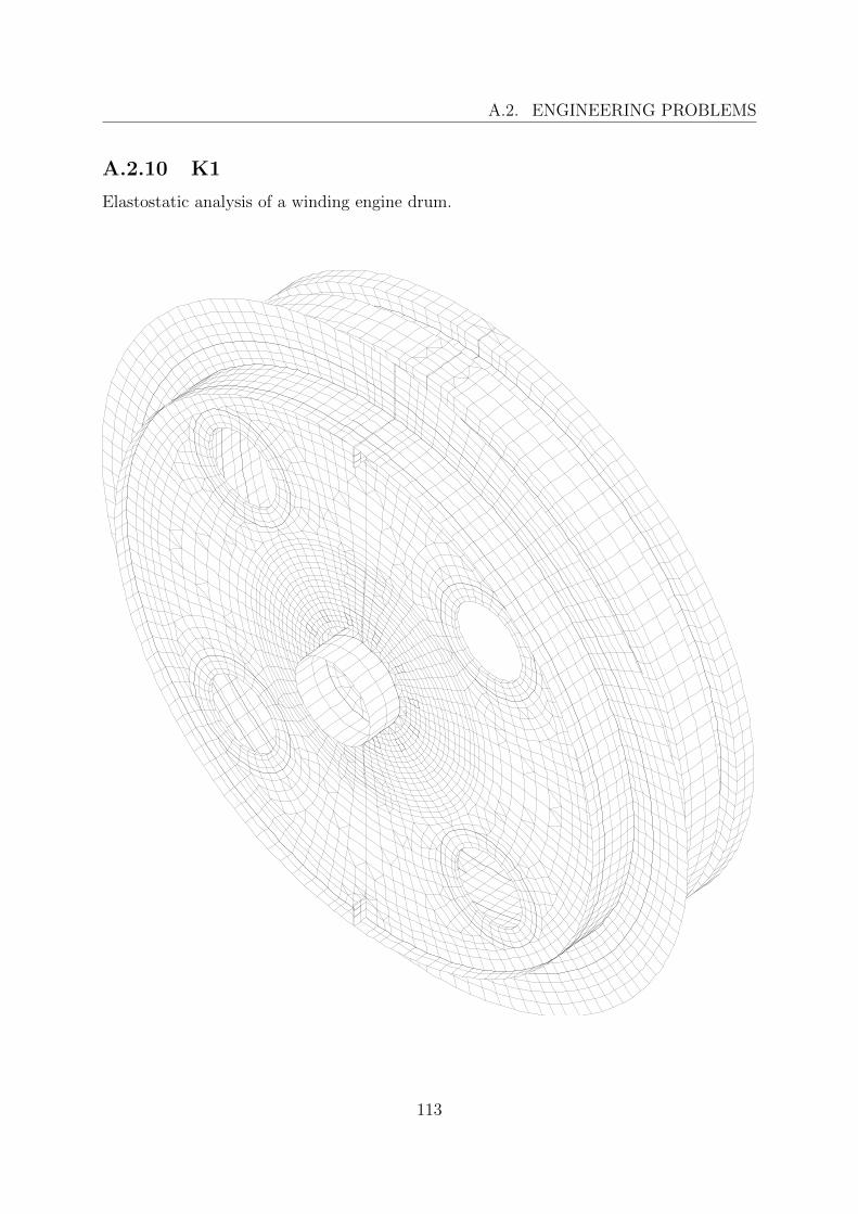
A.2. ENGINEERING PROBLEMS
A.2.10 K1
Elastostatic analysis of a winding engine drum.
113
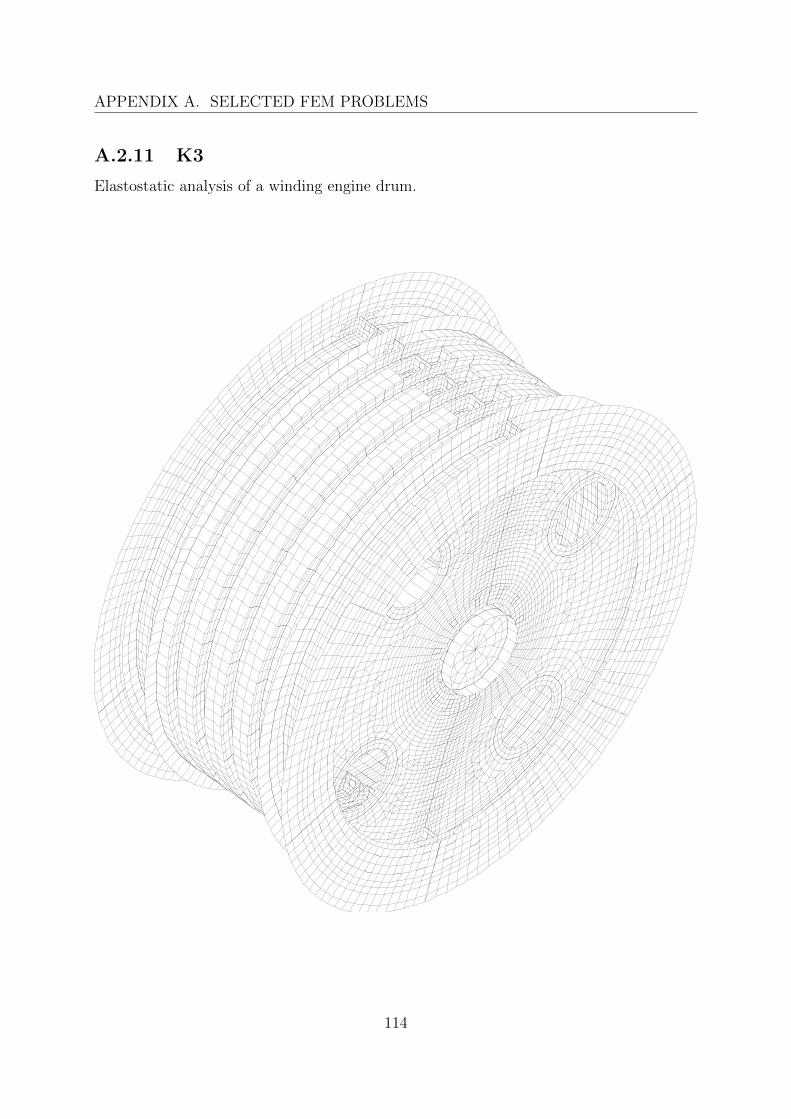
APPENDIX A. SELECTED FEM PROBLEMS
A.2.11 K3
Elastostatic analysis of a winding engine drum.
114
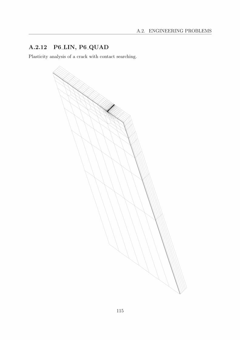
A.2. ENGINEERING PROBLEMS
A.2.12 P6 LIN, P6 QUAD
Plasticity analysis of a crack with contact searching.
115
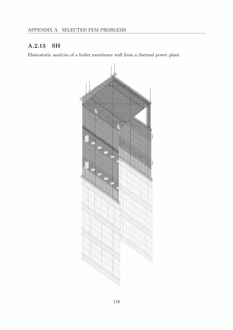
APPENDIX A. SELECTED FEM PROBLEMS
A.2.13 SH
Elastostatic analysis of a boiler membrane wall from a thermal power plant.
116
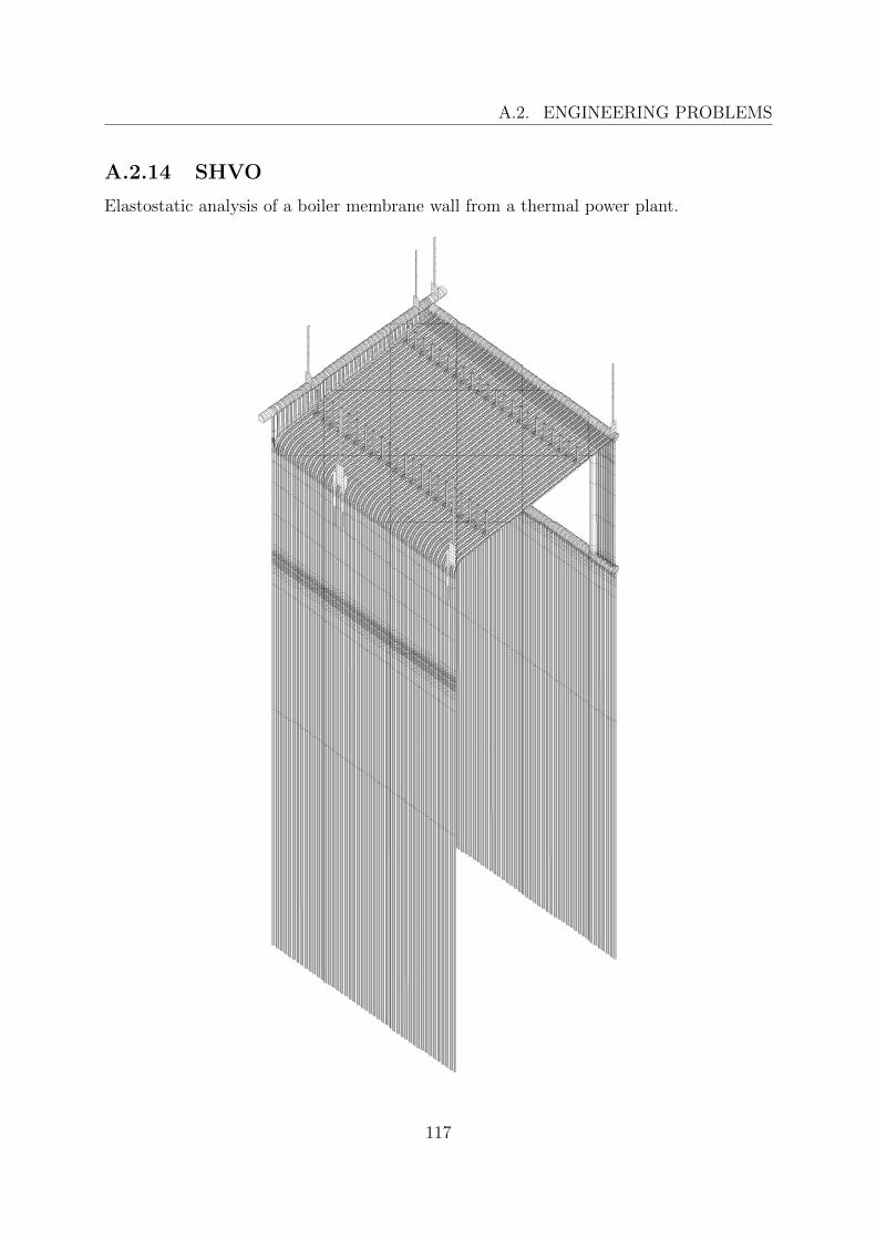
A.2. ENGINEERING PROBLEMS
A.2.14 SHVO
Elastostatic analysis of a boiler membrane wall from a thermal power plant.
117

Appendix B
Solver file formats
B.1 Formatted files
The only formatted files used by the sparse direct solver are the standard PMD input andoutput files. This section is intended to update the PMD Reference Guide.
B.1.1 name.I4 (FEFS, FESD)
The sparse direct solver utilizes the same input file as the frontal solver, i.e., name.I4,making it trivial for the user to move from one solver to the other. The correspondingoutput file is name.O4.
It is possible, if desired, to use several separate input and output files by adding anarbitrary alphanumeric character to the input file extension, i.e., name.I4A. The outputfile is also named accordingly.
Input file format
; integer parameters
IP KREST KMET KPRIN
; real parameters
RP PIVOT
; end of input
EN
EN
Description
KREST Restart key= 1 Factorize the coefficient matrix and solve for all load cases.= 2 Solve for additional load cases.
119
APPENDIX B. SOLVER FILE FORMATS
KMET Method key (controls minimum degree ordering algorithm)= 0 Use default method.= xx1 Compute exact degrees.= xx2 Compute approximate degrees according to Amestoy, Davis and Duff.= xx3 Compute approximate degrees according to Ashcraft, Eisenstat and Lucas.= xx4 Compute approximate degrees according to Gilbert, Moler and Schreiber.= x0x Do not preorder.= x1x Preorder with Cuthill-McKee algorithm.= x2x Preorder with reverse Cuthill-McKee algorithm.= 0xx Use supervariables with external degrees.= 1xx Use supervariables with true degrees.= 2xx Use true degrees (no supervariables).
KPRIN Print key (controls output to file name.O4)= 0 Do not print debug information (default).= 1 Print runtime and memory allocation information.= 2 Also print computed permutation vector.
PIVOT Minimum pivot value (default = 10−6)
Notes
• KREST has the same function in both solvers.
Necessary conditions for KREST = 2 are
– the program has already finished factorization with KREST = 1, and
– additional load cases were processed by programs RPD3 and SRH3 (or RPD2and SRH2, respectively) with KREST = 2.
• KMET is used only by the sparse direct solver.
The default value, recommended for general use, is KMET = 1. Other values mayoccasionally yield better orderings, but are usually slower.
Prefixing KMET with a minus sign causes the sparse direct solver to finish after theordering phase, giving the user the opportunity to check the computed ordering.KMET < 0 should be used together with KPRIN ≥ 1.
When solving very large problems, it may be worthwhile to test different degreecomputation methods and/or preordering methods this way to find the best suitedvalue of KMET before commiting the factorization, because savings in computationaltime and storage space may be significant.
• KPRIN is used only by the sparse direct solver.
120
B.2. UNFORMATTED FILES
• PIVOT has the same function in both solvers.
To prevent numerical instability, the factorization is stopped when the pivot in theabsolute value is too small (|p| ≤ PIVOT). A warning message is issued into theoutput file name.O4 whenever the pivot is negative or small (p ≤ 102 × PIVOT) tonotify the user. Such conditions are usually caused by errors in the input data.
B.2 Unformatted files
The sparse direct solver uses several intermediate unformatted files1 to store the coefficientmatrix factor (factorized equations) and other internal data. Intermediate files used bythe frontal solver are not accessed in any way. This section is intended only for PMDdevelopers.
B.2.1 IDEQC
File IDEQC is a sequential file used to store various internal data of the sparse direct solverrelated to ordering, assembly and factorization. It is written after the ordering phase andcontains four records:
1. Common parameters: NPIV, NVAR, NBLK1, NBLK2, SBUF1, SBUF2, LSMTX, LROW, LEMTXand KMET.
2. Permutation of nodes: array IPNOD(NNOD).
3. Permutation of degrees (equations): array IPSOL(LSOL).
4. Dimensions of matrix blocks: array MBD(NPIV).
B.2.2 IDEQI
File IDEQI is a sequential file used to store the indices of nonzero blocks in the factorizedcoefficient matrix, necessary to reconstruct the arrays MRP(NPIV+1) and MCI(NBLK2). Itis written during the ordering phase, but initially it contains unpermuted indices. Thefile is rewritten with correctly permuted indices prior to the assembly phase.
There are NPIV records; each record contains N+1 values of type INTEGER*4, where thefirst value is N , and the rest N values are indices of nonzero blocks in the correspondingcoefficient matrix block row.
1In the PMD documentation, unformatted files are commonly referred to by the corresponding sourcecode symbol consisting of prefix ID and the file extension, for example IDELM for file name.ELM.
121
APPENDIX B. SOLVER FILE FORMATS
B.2.3 IDEQR
File IDEQR is a direct-access file used to store the data of nonzero blocks in the coefficientmatrix factor. The internal structure is different from file IDEQ1 used by the frontal solver,therefore, equations factorized by the sparse direct solver cannot be directly used by thefrontal solver and vice versa.
The file is normally written after the factorization phase, however, in the out-of-coremode, it may be written as soon as during the assembly phase. There are NBLK2 records;each record represents one block (submatrix) and stores LBLK values of type REAL*8. Somespace is wasted in smaller blocks but an efficient out-of-core data manipulation is possible.
122
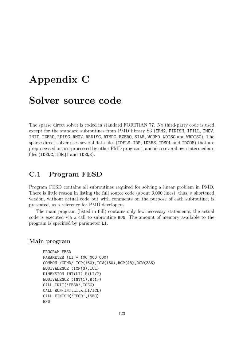
Appendix C
Solver source code
The sparse direct solver is coded in standard FORTRAN 77. No third-party code is usedexcept for the standard subroutines from PMD library S3 (ERM2, FINISH, IFILL, IMOV,INIT, IZERO, RDISC, RMOV, RRDISC, RTMPC, RZERO, SIAR, WCOMD, WDISC and WRDISC). Thesparse direct solver uses several data files (IDELM, IDP, IDRHS, IDSOL and IDCOM) that arepreprocessed or postprocessed by other PMD programs, and also several own intermediatefiles (IDEQC, IDEQI and IDEQR).
C.1 Program FESD
Program FESD contains all subroutines required for solving a linear problem in PMD.There is little reason in listing the full source code (about 3,000 lines), thus, a shortenedversion, without actual code but with comments on the purpose of each subroutine, ispresented, as a reference for PMD developers.
The main program (listed in full) contains only few necessary statements; the actualcode is executed via a call to subroutine RUN. The amount of memory available to theprogram is specified by parameter LI.
Main program
PROGRAM FESD
PARAMETER (LI = 100 000 000)
COMMON /CPMD/ ICP(160),ICW(160),RCP(48),RCW(336)
EQUIVALENCE (ICP(3),ICL)
DIMENSION INT(LI),R(LI/2)
EQUIVALENCE (INT(1),R(1))
CALL INIT(’FESD’,ISEC)
CALL RUN(INT,LI,R,LI/ICL)
CALL FINISH(’FESD’,ISEC)
END
123
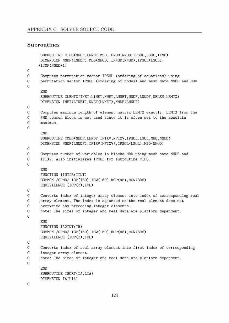
APPENDIX C. SOLVER SOURCE CODE
Subroutines
SUBROUTINE CIPS(NNDF,LNNDF,MBD,IPNOD,NNOD,IPSOL,LSOL,ITMP)
DIMENSION NNDF(LNNDF),MBD(NNOD),IPNOD(NNOD),IPSOL(LSOL),
*ITMP(NNOD+1)
C
C Computes permutation vector IPSOL (ordering of equations) using
C permutation vector IPNOD (ordering of nodes) and mesh data NNDF and MBD.
C
END
SUBROUTINE CLEMTX(INET,LINET,NNET,LNNET,NNDF,LNNDF,NELEM,LEMTX)
DIMENSION INET(LINET),NNET(LNNET),NNDF(LNNDF)
C
C Computes maximum length of element matrix LEMTX exactly. LEMTX from the
C PMD common block is not used since it is often set to the absolute
C maximum.
C
END
SUBROUTINE CMBD(NNDF,LNNDF,IFIXV,NFIXV,IPSOL,LSOL,MBD,NNOD)
DIMENSION NNDF(LNNDF),IFIXV(NFIXV),IPSOL(LSOL),MBD(NNOD)
C
C Computes number of variables in blocks MBD using mesh data NNDF and
C IFIXV. Also initializes IPSOL for subroutine CIPS.
C
END
FUNCTION IINT2R(IINT)
COMMON /CPMD/ ICP(160),ICW(160),RCP(48),RCW(336)
EQUIVALENCE (ICP(3),ICL)
C
C Converts index of integer array element into index of corresponding real
C array element. The index is adjusted so the real element does not
C overwrite any preceding integer elements.
C Note: The sizes of integer and real data are platform-dependent.
C
END
FUNCTION IR2INT(IR)
COMMON /CPMD/ ICP(160),ICW(160),RCP(48),RCW(336)
EQUIVALENCE (ICP(3),ICL)
C
C Converts index of real array element into first index of corresponding
C integer array element.
C Note: The sizes of integer and real data are platform-dependent.
C
END
SUBROUTINE ISORT(IA,LIA)
DIMENSION IA(LIA)
C
124
C.1. PROGRAM FESD
C Sorts elements of integer array IA using the insertion sort algorithm.
C
END
FUNCTION LINT2R(LINT)
COMMON /CPMD/ ICP(160),ICW(160),RCP(48),RCW(336)
EQUIVALENCE (ICP(3),ICL)
C
C Converts length of integer array into length of corresponding real array.
C Note: The sizes of integer and real data are platform-dependent.
C
END
FUNCTION LR2INT(LR)
COMMON /CPMD/ ICP(160),ICW(160),RCP(48),RCW(336)
EQUIVALENCE (ICP(3),ICL)
C
C Converts length of real array into length of corresponding integer array.
C Note: The sizes of integer and real data are platform-dependent.
C
END
SUBROUTINE PADD(IA,IB,LIAB)
DIMENSION IA(LIAB),IB(LIAB)
C
C Combines two successive permutations defined by vectors IA and IB into
C a single permutation vector and stores the result back in array IA.
C
END
SUBROUTINE PIAR(IA,IB,IP,LIABP)
DIMENSION IA(LIABP),IB(LIABP),IP(LIABP)
C
C Permutes integer array IA using permutation vector IP and stores the
C result in array in IB.
C
END
SUBROUTINE PIARR(IA,IB,IP,LIABP)
DIMENSION IA(LIABP),IB(LIABP),IP(LIABP)
C
C Permutes integer array IA using inverse permutation vector IP and stores
C the result in array in IB. Permutation is done without computing the
C inverse.
C
END
SUBROUTINE PINV(IA,IB,LIAB)
DIMENSION IA(LIAB),IB(LIAB)
C
C Computes inverse transformation (ordering) to IA and stores it in IB.
C
125
APPENDIX C. SOLVER SOURCE CODE
END
SUBROUTINE PRAR(A,B,IP,LABP)
DIMENSION A(LABP),B(LABP),IP(LABP)
C
C Permutes real array A using permutation vector IP and stores the result
C in array in B.
C
END
SUBROUTINE PRARR(A,B,IP,LABP)
DIMENSION A(LABP),B(LABP),IP(LABP)
C
C Permutes real array A using inverse permutation vector IP and stores the
C result in array in B. Permutation is done without computing the inverse.
C
END
SUBROUTINE RUN(INT,LI,R,LR)
COMMON /CPMD/ ICP(160),ICW(160),RCP(48),RCW(336)
EQUIVALENCE (ICP(1),MW),(ICP(3),ICL),(ICP(10),NELEM),
*(ICP(11),NNOD),(ICP(18),LINET),(ICP(19),LNNET),(ICP(20),LNNDF),
*(ICP(28),NFIXV),(ICP(34),LSOL),(ICP(62),IDP),(ICP(63),IDCOM),
*(ICP(66),IDELM),(ICP(67),IDRHS),(ICP(73),IDSOL),(ICP(84),NASV),
*(ICP(86),KPRIN),(ICP(122),KFES)
EQUIVALENCE (ICW(1),NPIV),(ICW(2),NVAR),(ICW(3),NBLK1),
*(ICW(4),NBLK2),(ICW(5),LSMTX),(ICW(6),LEMTX),(ICW(7),LROW),
*(ICW(8),IDEQC),(ICW(9),IDEQI),(ICW(10),IDEQR),(ICW(11),LBBUF),
*(ICW(12),LEBUF),(ICW(13),LCBUF)
EQUIVALENCE (RCW(1),SBUF1),(RCW(2),SBUF2)
DIMENSION INT(LI),R(LR)
C
C Manages the operation of the sparse direct solver.
C
END
SUBROUTINE SDAMD(IG,LIG,ID,IS,IN,IP,MBD,IPNOD,ITMP,JTMP,KTMP,
*NBLK,SBUF,LROW,IDISC,KDG,KSV,KED)
COMMON /CPMD/ ICP(160),ICW(160),RCP(48),RCW(336)
EQUIVALENCE (ICP(1),MW),(ICP(11),NNOD),(ICP(86),KPRIN),
*(ICP(132),KMET)
DIMENSION MBD(NNOD),IPNOD(NNOD),ITMP(NNOD),JTMP(NNOD),
*KTMP(NNOD),IG(LIG),ID(NNOD),IS(NNOD),IN(NNOD),IP(NNOD)
C
C Computes permutation vector IPNOD (ordering of nodes) using minimum degree
C ordering algorithm. Also computes memory requirements for factorization
C and writes indices of nonzero matrix blocks into file IDEQI.
C
END
SUBROUTINE SDASM(MRP,MCI,MBP,BUF,IPSOL,INET,NNET,NNDF,ITMP,TMP,
126
C.1. PROGRAM FESD
*SBUF)
COMMON /CPMD/ ICP(160),ICW(160),RCP(48),RCW(336)
EQUIVALENCE (ICP(1),MW),(ICP(3),ICL),(ICP(10),NELEM),
*(ICP(11),NNOD),(ICP(18),LINET),(ICP(19),LNNET),(ICP(20),LNNDF),
*(ICP(34),LSOL),(ICP(66),IDELM),(ICP(86),KPRIN)
EQUIVALENCE (ICW(1),NPIV),(ICW(2),NVAR),(ICW(3),NBLK1),
*(ICW(4),NBLK),(ICW(6),LEMTX),(ICW(11),LBBUF),(ICW(12),LEBUF),
*(ICW(14),NA),(ICW(15),NR),(ICW(16),NW),(ICW(17),NF)
DIMENSION MRP(NPIV+1),MCI(NBLK),MBP(NBLK),BUF(LEBUF),
*IPSOL(LSOL),INET(LINET),NNET(LNNET),NNDF(LNNDF),
*ITMP(NNOD),TMP(LEMTX),NDF(20),IDF(20)
C
C Assembles the coefficient matrix using element matrices from file IDELM.
C
END
SUBROUTINE SDBKS(MRP,MCI,MBP,MBD1,BUF,RHS,LRHS,NRHS)
COMMON /CPMD/ ICP(160),ICW(160),RCP(48),RCW(336)
EQUIVALENCE (ICW(1),NPIV),(ICW(2),NVAR),(ICW(4),NBLK),
*(ICW(12),LEBUF)
DIMENSION MRP(NPIV+1),MCI(NBLK),MBP(NBLK),MBD1(NPIV+1),
*BUF(LEBUF),RHS(LRHS,NRHS)
C
C Performs back substitution for all right-hand sides RHS. The result is
C stored back in RHS.
C
END
SUBROUTINE SDBUF1(MRP,MCI,MBP,BUF,IPSOL,NNDF,ITMP,
*IBLK,LBLK,IPTR)
COMMON /CPMD/ ICP(160),ICW(160),RCP(48),RCW(336)
EQUIVALENCE (ICP(11),NNOD),(ICP(20),LNNDF),(ICP(34),LSOL)
EQUIVALENCE (ICW(1),NPIV),(ICW(2),NVAR),(ICW(4),NBLK),
*(ICW(10),IDEQR),(ICW(11),LBBUF),(ICW(12),LEBUF),(ICW(13),LCBUF),
*(ICW(14),NA),(ICW(16),NW),(ICW(17),NF),(ICW(15),NR)
DIMENSION MRP(NPIV+1),MCI(NBLK),MBP(NBLK),BUF(LEBUF),
*IPSOL(LSOL),NNDF(LNNDF),ITMP(NNOD)
C
C Adds submatrix to buffer BUF (optionally first reads matrix block from
C file IDEQR). When the buffer is full, writes all matrix blocks into file
C IDEQR and resets the buffer.
C
END
SUBROUTINE SDBUF2(MRP,MCI,MBP,MBD,BUF,ITMP,IPIV,IROW)
COMMON /CPMD/ ICP(160),ICW(160),RCP(48),RCW(336)
EQUIVALENCE (ICW(1),NPIV),(ICW(4),NBLK),(ICW(10),IDEQR),
*(ICW(11),LBBUF),(ICW(12),LEBUF),(ICW(13),LCBUF),
*(ICW(14),NR),(ICW(15),NW),(ICW(16),NF)
127
APPENDIX C. SOLVER SOURCE CODE
DIMENSION MRP(NPIV+1),MCI(NBLK),MBP(NBLK),MBD(NPIV),BUF(LEBUF),
*ITMP(NPIV)
C
C Reads row of matrix blocks from file IDEQR into buffer BUF. When the
C buffer is full, writes all matrix blocks into file IDEQR and resets the
C buffer.
C
END
SUBROUTINE SDBUF3(MBP,BUF,IBLK,LBLK)
COMMON /CPMD/ ICP(160),ICW(160),RCP(48),RCW(336)
EQUIVALENCE (ICW(4),NBLK),(ICW(10),IDEQR),(ICW(11),LBBUF),
*(ICW(12),LEBUF),(ICW(13),LCBUF),(ICW(14),NR),(ICW(15),NF)
DIMENSION MBP(NBLK),BUF(LEBUF)
C
C Reads matrix block from file IDEQR into buffer BUF. When the buffer is
C full, resets the buffer.
C
END
SUBROUTINE SDCHK(LI,LMAX,LCOR,LBUF)
COMMON /CPMD/ ICP(160),ICW(160),RCP(48),RCW(336)
EQUIVALENCE (ICP(1),MW),(ICP(86),KPRIN)
C
C Checks memory requirement LMAX against available memory LI. If the
C available memory is insufficient the program is aborted.
C
END
SUBROUTINE SDDIS(MRP,MCI,MBP,MBD1,BUF,RHS,TMP,SBUF)
COMMON /CPMD/ ICP(160),ICW(160),RCP(48),RCW(336)
EQUIVALENCE (ICP(1),MW),(ICP(3),ICL),(ICP(34),LSOL),
*(ICP(84),NASV),(ICP(86),KPRIN)
EQUIVALENCE (ICW(1),NPIV),(ICW(2),NVAR),(ICW(4),NBLK),
*(ICW(11),LBBUF),(ICW(12),LEBUF),(ICW(14),NR),(ICW(15),NF)
DIMENSION MRP(NPIV+1),MCI(NBLK),MBP(NBLK),MBD1(NPIV+1),
*BUF(LEBUF),RHS(LSOL,NASV),TMP(NVAR)
C
C Computes solution for all right-hand sides RHS using forward and back
C substitution. The result is stored back in RHS.
C
END
SUBROUTINE SDFAC(MRP,MCI,MBP,MBD,BUF,ITMP,SBUF)
COMMON /CPMD/ ICP(160),ICW(160),RCP(48),RCW(336)
EQUIVALENCE (ICP(1),MW),(ICP(3),ICL),(ICP(86),KPRIN)
EQUIVALENCE (ICW(1),NPIV),(ICW(4),NBLK),(ICW(10),IDEQR),
*(ICW(11),LBBUF),(ICW(12),LEBUF),
*(ICW(14),NR),(ICW(15),NW),(ICW(16),NF)
DIMENSION MRP(NPIV+1),MCI(NBLK),MBP(NBLK),MBD(NPIV),BUF(LEBUF),
128
C.1. PROGRAM FESD
*ITMP(NPIV),D(6),G(6,6)
C
C Factorizes the coefficient matrix. The factor is stored in the place of
C the original matrix.
C
END
SUBROUTINE SDFWS(MRP,MCI,MBP,MBD1,BUF,RHS,LRHS,NRHS,TMP)
COMMON /CPMD/ ICP(160),ICW(160),RCP(48),RCW(336)
EQUIVALENCE (ICW(1),NPIV),(ICW(2),NVAR),(ICW(4),NBLK),
*(ICW(12),LEBUF)
DIMENSION MRP(NPIV+1),MCI(NBLK),MBP(NBLK),MBD1(NPIV+1),
*BUF(LEBUF),RHS(LRHS,NRHS),TMP(NVAR)
C
C Performs forward substitution for all right-hand sides RHS. The result is
C stored back in RHS.
C
END
SUBROUTINE SDGRF(IG,LIG,INET,NNET,MBD,NBLK,SBUF)
COMMON /CPMD/ ICP(160),ICW(160),RCP(48),RCW(336)
EQUIVALENCE (ICP(10),NELEM),(ICP(11),NNOD),(ICP(18),LINET),
*(ICP(19),LNNET)
DIMENSION IG(LIG),INET(LINET),NNET(LNNET),MBD(NNOD)
C
C Constructs a quotient graph for the minimum degree ordering algorithm and
C computes memory requirements for the assembly.
C
END
SUBROUTINE SDORD(IG,LIG,INET,NNET,MBD,IPNOD,IPNOD1,ITMP,
*KPR,KED,KSV,KDG)
COMMON /CPMD/ ICP(160),ICW(160),RCP(48),RCW(336)
EQUIVALENCE (ICP(1),MW),(ICP(11),NNOD),(ICP(18),LINET),
*(ICP(19),LNNET),(ICP(86),KPRIN)
EQUIVALENCE (ICW(3),NBLK1),(ICW(4),NBLK2),(ICW(7),LROW),
*(ICW(9),IDEQI)
EQUIVALENCE (RCW(1),SBUF1),(RCW(2),SBUF2)
DIMENSION IG(LIG),INET(LINET),NNET(LNNET),MBD(NNOD),
*IPNOD(NNOD),IPNOD1(NNOD),ITMP(NNOD*3)
C
C Preorders nodes using subroutine SDRCM (if requested) and then calculates
C permutation vector IPNOD using subroutine SDAMD.
C
END
SUBROUTINE SDPIV(PIVOT,DIAG,ISOL)
COMMON /CPMD/ ICP(160),ICW(160),RCP(48),RCW(336)
EQUIVALENCE (ICP(1),MW)
EQUIVALENCE (RCP(32),PIVAL)
129
APPENDIX C. SOLVER SOURCE CODE
C
C Checks pivot value PIVOT of equation ISOL and stores its reciprocal value
C in DIAG. If the pivot is equal or less than PIVAL the program is aborted.
C
END
SUBROUTINE SDPMI(MRP,NPIV,MCI,NBLK,IPNOD,NNOD)
DIMENSION MRP(NPIV+1),MCI(NBLK),IPNOD(NNOD)
C
C Permutes column indices of matrix blocks MCI using permutation vector
C IPNOD (ordering of nodes).
C
END
SUBROUTINE SDPPV(IG,LIG,ID,KQ,KL,IROOT)
COMMON /CPMD/ ICP(160),ICW(160),RCP(48),RCW(336)
EQUIVALENCE (ICP(11),NNOD)
DIMENSION IG(LIG),ID(NNOD),KQ(NNOD),KL(NNOD)
C
C Calculates the pseudo-peripheral vertex of the ordering graph starting
C at vertex IROOT. The pseudo-peripheral vertex is returned in IROOT.
C
END
SUBROUTINE SDRCM(IG,LIG,ID,IPNOD,ITMP,KPR)
COMMON /CPMD/ ICP(160),ICW(160),RCP(48),RCW(336)
EQUIVALENCE (ICP(11),NNOD),(ICP(86),KPRIN)
DIMENSION IG(LIG),ID(NNOD),IPNOD(NNOD),ITMP(NNOD)
C
C Computes permutation vector IPNOD (ordering of nodes) using Cuthill-McKee
C ordering algorithm. Reverse algorithm is used if KPR is nonzero.
C
END
SUBROUTINE SDREF(INET,NNET,NNDF,IPSOL,SOL,REF,ITMP,TMP)
COMMON /CPMD/ ICP(160),ICW(160),RCP(48),RCW(336)
EQUIVALENCE (ICP(10),NELEM),(ICP(11),NNOD),(ICP(18),LINET),
*(ICP(19),LNNET),(ICP(20),LNNDF),(ICP(34),LSOL),(ICP(66),IDELM),
*(ICP(84),NASV)
EQUIVALENCE (ICW(2),NVAR),(ICW(6),LEMTX)
DIMENSION INET(LINET),NNET(LNNET),NNDF(LNNDF),IPSOL(LSOL),
*SOL(LSOL,NASV),REF(LSOL,NASV),ITMP(NNOD),TMP(LEMTX),IS(60)
C
C Computes reaction forces REF for all load cases SOL. Corresponding
C equations are assembled from file IDELM.
C
END
SUBROUTINE SDREQ(CMIN,CMAX,DMAX,KPR)
COMMON /CPMD/ ICP(160),ICW(160),RCP(48),RCW(336)
EQUIVALENCE (ICP(1),MW),(ICP(3),ICL),(ICP(11),NNOD),
130
C.2. PROGRAM FESDA
*(ICP(18),LINET),(ICP(19),LNNET),(ICP(20),LNNDF),(ICP(28),NFIXV),
*(ICP(34),LSOL),(ICP(84),NASV),(ICP(86),KPRIN)
EQUIVALENCE (ICW(1),NPIV),(ICW(2),NVAR),(ICW(3),NBLK1),
*(ICW(4),NBLK2),(ICW(5),LSMTX),(ICW(6),LEMTX),(ICW(7),LROW)
EQUIVALENCE (RCW(1),SBUF1),(RCW(2),SBUF2)
C
C Calculates the memory requirements of the sparse direct solver.
C
END
SUBROUTINE SDRMI(MRP,NPIV,MCI,NBLK,IDISC)
DIMENSION MRP(NPIV+1),MCI(NBLK)
C
C Reads the indices of the matrix blocks from file IDISC.
C
END
SUBROUTINE SDWMI(MRP,NPIV,MCI,NBLK,IDISC)
DIMENSION MRP(NPIV+1),MCI(NBLK)
C
C Writes the indices of the matrix blocks into file IDISC.
C
END
C.2 Program FESDA
Since the recompilation of the source code in order to change parameter LI is usuallynot feasible to normal user, program FESDA, which uses dynamic memory allocation, isalso available. The program differs only in the main program code, all subroutines areidentical to program FESD. It requires a Fortran 90 compiler, however, the compilationneeds to be done only once.
To change the default value of LI, use additional parameters on the command line:
FESDA name -MLI value
where name is the name of problem data and value is the requested value of LI. Thevalue can be specified also in megabytes (220 bytes) using parameter -M instead of -MLI.If the specified value is 0, all available memory is allocated, subject to the limits of thecompiler, operating system and computer configuration.
131