Turk J Elec Eng & Comp Sci

(2017) 25: 844 – 861

c⃝ TUBITAK

doi:10.3906/elk-1411-129

Turkish Journal of Electrical Engineering & Computer Sciences

http :// journa l s . tub i tak .gov . t r/e lektr ik/

Research Article

An optimized buffer insertion algorithm with delay-power constraints for VLSI

layouts

Chessda UTTRAPHAN1,∗, Nasir SHAIKH-HUSIN2, Mohamed KHALIL-HANI21Embedded Computing System (EmbCoS) Research Focus Group, Department of Computer Engineering,

Faculty of Electrical and Electronic Engineering, Universiti Tun Hussein Onn Malaysia, Batu Pahat, Malaysia2Universiti Teknologi Malaysia, Johor Bahru, Malaysia

Received: 19.11.2014 • Accepted/Published Online: 03.03.2016 • Final Version: 10.04.2017

Abstract: We propose a grid-graph algorithm for interconnect routing and buffer insertion in nanometer VLSI layout

designs. The algorithm is designed to handle multiconstraint optimizations, namely timing performance and power

dissipation. The proposed algorithm is called HRTB-LA, which stands for hybrid routing tree and buffer insertion with

look-ahead. In recent VLSI designs, interconnect delay has become a dominant factor compared to gate delay. The

well-known technique to minimize the interconnect delay is by inserting buffers along the interconnect wires. However,

the buffer itself consumes power and it has been shown that power dissipation overhead due to buffer insertions is

significantly high. Many methodologies to optimize timing performance with power constraint have been proposed,

and no algorithm is based on dynamic programing technique using a grid graph. In addition, most of the algorithms

for buffer insertion use a postrouting buffer insertion approach. In the presence of buffer obstacles, these postrouting

algorithms may produce poor solutions. On the other hand, the simultaneous routing and buffer insertion algorithm

offers a better solution, but it was proven to be NP complete. Hence, our main contribution is an efficient algorithm

using a hybrid approach for multiconstraint optimization for multisink nets. The algorithm uses dynamic programming

to compute incrementally the interconnect delay and power dissipation of the inserted buffers while an effective runtime

is achieved with the aid of novel look-ahead and graph pruning schemes. Experimental results prove that HRTB-LA is

able to handle multiconstraint optimizations and produces a solution up to 30% better compared to a postrouting buffer

insertion algorithm in comparable runtime.

Key words: Buffer insertion, dynamic programming, VLSI routing optimization, VLSI design automation, power

dissipation

1. Introduction

The demand for high speed and low power consumption in today’s applications has forced dramatic changes

in the design and manufacturing methodologies for very large scale integration (VLSI) circuits [1]. To meet

the demand, the number of devices (i.e. transistors) on a single chip must be increased and this will lead to

a decrease in the device size and also will need a larger layout area to support huge amounts of devices. As

the size of the device decreases and it operates at a higher speed, the interconnect delay becomes much more

significant compared to the device delay. The interconnect delay increases quadratically with the length of the

wire [2].

An effective technique to reduce the interconnect delay is by inserting a buffer to reconstruct the signal

∗Correspondence: chessda@uthm.edu.my

844

UTTRAPHAN et al./Turk J Elec Eng & Comp Sci

along the interconnect tree. A systematic technique was proposed by van Ginneken [2]. Given the possible

buffer locations, van Ginneken’s algorithm can find the optimum buffering solution for the fixed signal routing

tree that maximizes timing slack at the source according to the Elmore delay model [2,3]. The algorithm applied

dynamic programming [4,5] to compute the slack iteratively from the sink nodes to the source node. As design

dimensions continue to shrink, more and more buffers are needed to improve the timing performance. However,

the buffer itself consumes power [6]. Saxena et al. [7] predicted that the total block cell count made up of buffers

will reach 35% in the 45-nm technology node and 70% in 32-nm technology. It has also been found that power

dissipation overhead due to optimal buffer insertion is significantly high and can be as high as 20% of total chip

power dissipation [6]. Therefore, the buffer insertion algorithm should be able to handle the power dissipation

constraint [1,6,8]. Many closed-form solutions for optimizing timing performance and power constraint have

been proposed [6,8,9], but none of them can be integrated into a buffer insertion algorithm that is based on

dynamic programming using a grid graph technique.

As the number of buffers inserted in the circuits increases dramatically, an algorithm that is fast and

efficient is essential for the design automation tools. Recently, many techniques to speed up van Ginneken’s

algorithm and its extensions were proposed. Shi and Li [10–13] improved the time complexity of van Ginneken’s

algorithm by introducing four novel techniques: predictive pruning, candidate tree, fast redundancy check, and

fast merging. Their algorithm is called FBI for fast buffer insertion. However, these algorithms (also known

as two-step or postrouting algorithms) are not designed to handle obstacles. In today’s VLSI design, some

regions may be occupied by predesigned libraries such as IP blocks and memory arrays. Some of these regions

do not allow buffer placement or wire to pass through and some regions only allow wire to go through but are

restricted for any buffer insertion. Therefore, in order to obtain a better solution, buffer insertion should be

performed taking into account these buffer and wire obstacles. In other words, the routing should be performed

simultaneously with buffer insertion. Zhou et al. [14] proposed a simultaneous algorithm for two-pin (one sink)

nets while for multisink nets Cong and Yuan [15] proposed an algorithm called RMP (recursive merging and

pruning) to solve the same problem. However, these types of algorithms are proven to be NP-complete because

the search space is too big [16]. The efficiency of Zhou’s algorithm is improved by S-RABILA (simultaneous

routing and buffer insertion with look-ahead) algorithm [17] using a novel technique called look-ahead but their

algorithm is limited to single sink problems.

Hu et al. [18] proposed a heuristic algorithm to solve multipin nets by constructing a performance-driven

Steiner tree and creating an alternative Steiner node if the original Steiner node is inside the obstacle area.

This two-step approach can achieve a better quality solution than van Ginneken’s algorithm (and its extensions)

because the initial tree is modified according to the needs for buffer insertion. The algorithm is called RIATA

for repeater insertion with adaptive tree adjustment. RIATA is very fast because it operates on a fixed tree but

the solution quality may not be good enough if many paths of the adjusted tree still overlap with the buffer

obstacles.

In this paper, we propose a graph based technique called hybrid routing tree and buffer insertion with

look-ahead (HRTB-LA). Instead of a fixed routing tree as in van Ginneken’s algorithm, FBI, and RIATA, we

use maze routing to find the solution. However, HRTB-LA will not explore the entire graph as in RMP because

we use the initial tree as a reference for determining the Steiner node as in RIATA. We also incorporate the

technique of graph pruning and look-ahead from [17,19], which is proven to be fast in single sink nets, into the

multisink nets problem. The remainder of this paper is organized as follows: Section 2 describes the theoretical

background for buffer insertion algorithms while Section 3 describes the problem formulation. Section 4 presents

845

UTTRAPHAN et al./Turk J Elec Eng & Comp Sci

the modelling of the proposed algorithm. Section 5 discusses the detail descriptions of the proposed HRTB-LA

algorithm. The results and analysis are discussed in Section 6. The final section concludes the paper.

2. Background

In this work, simultaneous routing and buffer insertion is formulated as a shortest-path problem in a weighted

graph specified as follows. Given a routing grid graph G = (V , E) corresponding to VLSI layout where v ∈ V

and e ∈ E is a set of internal vertices and a set of internal edges, respectively, a source node S0 ∈ V , n sink

nodes s1 , s2 , . . . , sn ∈ V , n – 1 Steiner nodes m1 , m2 , . . . , mn−1 ∈ V , required arrival time, RAT(s1),

RAT(s2), . . . , RAT(sn), a power constraint pc , a buffer library B , and a wire parameter W . The goal is to

find a new routing tree simultaneously with buffer insertion such that the slack at source and power dissipation

of buffers satisfy the given constraints. A vertex vi ∈ V may belong to the set of buffer obstacle vertices,

denoted as VOB , or a set of wire obstacle vertices, denoted as VOW . A buffer library B contains different types

of buffer. For each edge e = u → v , the signal travels from u to v , where u is the upstream vertex and v is

the downstream vertex and u , v /∈ VoW .

This section presents the fundamental background of buffer insertion algorithms ranging from basic buffer

insertion algorithm to the advance optimization techniques such as simultaneous routing and buffer insertion,

and multiconstraint optimization techniques.

2.1. Classic buffer insertion algorithm

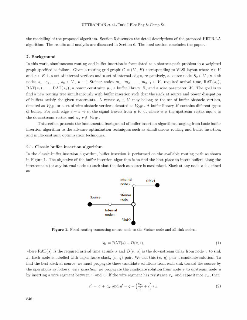
In the classic buffer insertion algorithm, buffer insertion is performed on the available routing path as shown

in Figure 1. The objective of the buffer insertion algorithm is to find the best place to insert buffers along the

interconnect (at any internal node v) such that the slack at source is maximized. Slack at any node v is definedas

Figure 1. Fixed routing connecting source node to the Steiner node and all sink nodes.

qv = RAT(s)−D(v, s), (1)

where RAT(s) is the required arrival time at sink s and D(v , s) is the downstream delay from node v to sink

s . Each node is labelled with capacitance-slack, (c , q) pair. We call this (c , q) pair a candidate solution. To

find the best slack at source, we must propagate these candidate solutions from each sink toward the source by

the operations as follows: wire insertion, we propagate the candidate solution from node v to upstream node u

by inserting a wire segment between u and v . If the wire segment has resistance rw and capacitance cw , then

c′ = c + cw and q′ = q −(cw

2+ c)rw, (2)

846

UTTRAPHAN et al./Turk J Elec Eng & Comp Sci

where c ’ and q ’ are the accumulated capacitance and accumulated slack from sink respectively for node u . In

buffer insertion, we insert a buffer at node u and add a new candidate to the solution set. If a buffer b has

input capacitance cb , output resistance rb , and intrinsic delay db , then the new candidate is

c′ = cb and q′ = q − rbc− db. (3)

In branch merging, when the solution sets reach a Steiner node, the solutions from the left child of the Steiner

node are merged with solutions from the right child of the Steiner node. If the left candidate is (c , q)left and

the right candidate is (c , q)right , the merging solution is given by

c′ = cleft + cright and q′ = min(qleft, qright). (4)

In pruning, we apply the following criterion: for any two candidate solutions at node v , β1 = (c1 , q1) is

dominated by β2 = (c2 , q2) if c1 ≥ c2 and q1 ≤ q2 . When a candidate solution reaches the source node, the

slack at source is computed considering the source resistance, Rs , as follows:

qsource = q − cRs. (5)

For illustration, we use the following parameter values: load capacitance CL at sink node is 0.022 pF, wire

resistance rw is 37.5 Ω per segment, wire capacitance cw is 0.1026 pF per segment, buffer input capacitance

cb is 0.022 pF, buffer output resistance rb is 104.2 Ω, buffer intrinsic delay db is 20 ps, and the source output

resistance Rs is 104.2 Ω. Assume that the required arrival time (RAT) for each sink is 200 ps. The solution

for the interconnect tree in Figure 1 is shown in Figure 2.

Figure 2. Candidate solutions at each node. The red color is the best solution for the given path.

The path expansion starts from a sink node, for example the top sink node, where the (c , q) pair is

(0.022, 200), to the next node. By inserting a wire using Eq. (2), the subsequent candidate solution is therefore

(0.125, 197.25). Next, the buffer is inserted using Eq. (3) to obtain another solution, which is (0.022, 164.27).

These are the possible solutions at the node next to the sink node. These operations are applied for all sink

nodes. These solutions will grow as the solutions are propagated toward the source as shown in Figure 2. When

the source is reached, the final solution is computed using Eq. (5). In this example, the best solution is 110.02

ps and the buffer is inserted at the Steiner node.

2.2. Simultaneous routing and buffer insertion for tree topology

Simultaneous routing and buffer insertion for tree topology is performed by utilizing a maze search algorithm

[5,20,21]. In this type of algorithm, the VLSI circuit is represented by a uniform 2D grid graph and the source

847

UTTRAPHAN et al./Turk J Elec Eng & Comp Sci

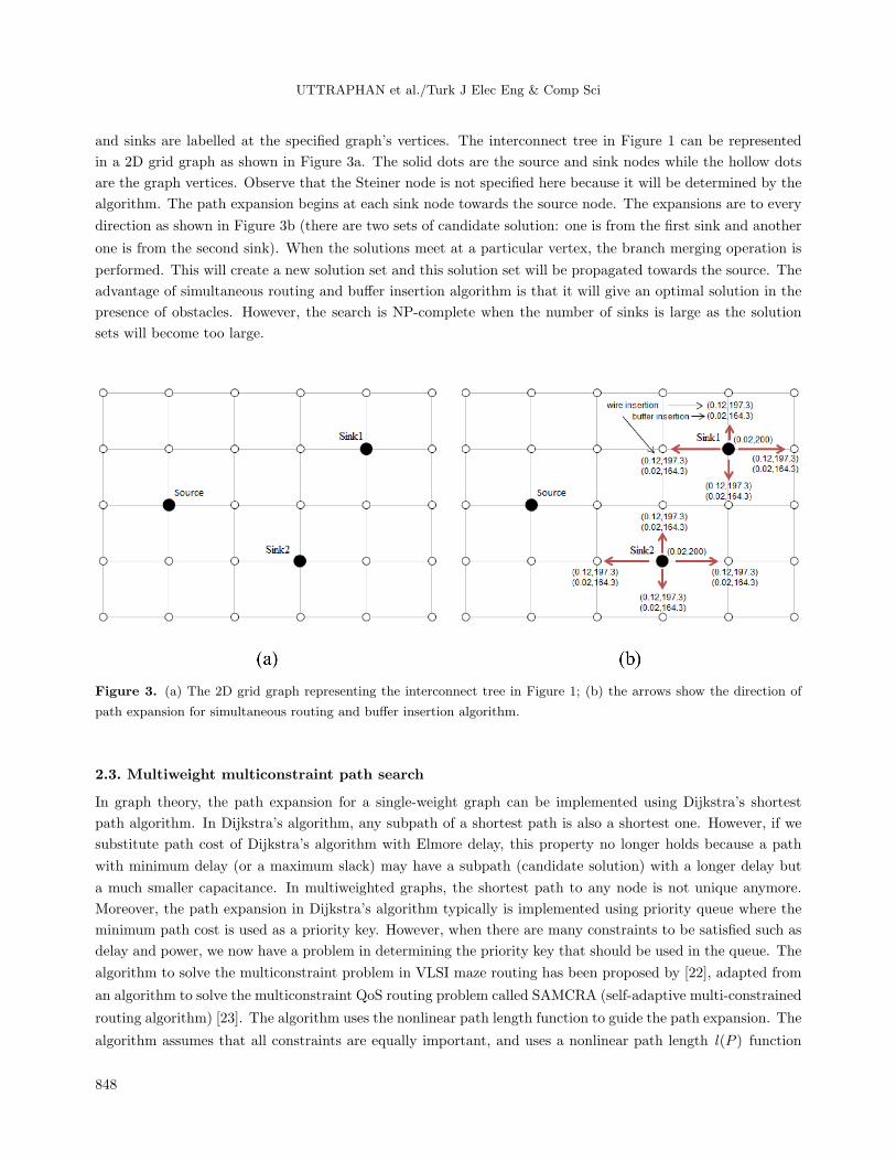
and sinks are labelled at the specified graph’s vertices. The interconnect tree in Figure 1 can be represented

in a 2D grid graph as shown in Figure 3a. The solid dots are the source and sink nodes while the hollow dots

are the graph vertices. Observe that the Steiner node is not specified here because it will be determined by the

algorithm. The path expansion begins at each sink node towards the source node. The expansions are to every

direction as shown in Figure 3b (there are two sets of candidate solution: one is from the first sink and another

one is from the second sink). When the solutions meet at a particular vertex, the branch merging operation is

performed. This will create a new solution set and this solution set will be propagated towards the source. The

advantage of simultaneous routing and buffer insertion algorithm is that it will give an optimal solution in the

presence of obstacles. However, the search is NP-complete when the number of sinks is large as the solution

sets will become too large.

Figure 3. (a) The 2D grid graph representing the interconnect tree in Figure 1; (b) the arrows show the direction of

path expansion for simultaneous routing and buffer insertion algorithm.

2.3. Multiweight multiconstraint path search

In graph theory, the path expansion for a single-weight graph can be implemented using Dijkstra’s shortest

path algorithm. In Dijkstra’s algorithm, any subpath of a shortest path is also a shortest one. However, if we

substitute path cost of Dijkstra’s algorithm with Elmore delay, this property no longer holds because a path

with minimum delay (or a maximum slack) may have a subpath (candidate solution) with a longer delay but

a much smaller capacitance. In multiweighted graphs, the shortest path to any node is not unique anymore.

Moreover, the path expansion in Dijkstra’s algorithm typically is implemented using priority queue where the

minimum path cost is used as a priority key. However, when there are many constraints to be satisfied such as

delay and power, we now have a problem in determining the priority key that should be used in the queue. The

algorithm to solve the multiconstraint problem in VLSI maze routing has been proposed by [22], adapted from

an algorithm to solve the multiconstraint QoS routing problem called SAMCRA (self-adaptive multi-constrained

routing algorithm) [23]. The algorithm uses the nonlinear path length function to guide the path expansion. The

algorithm assumes that all constraints are equally important, and uses a nonlinear path length l(P ) function

848

UTTRAPHAN et al./Turk J Elec Eng & Comp Sci

defined as

l(P ) = max1≤i≤n

[wi(P )

Li

], (6)

where w(P ), L , and n are weight vector for path P , constraint vector, and the total number of constraints,

respectively. The SAMCRA routing algorithm computes the path P that obeys multiple constraints wi(P ) ≤ Li

for all 1 ≤ i ≤ n . As an example, we want to seek a path for which the source-to-sink (two-pin net) delay is

less than 100 ps (L1) and the total power dissipation of the inserted buffers along the path must not exceed 2

mW (L2). Li are the constraints set by the user. Suppose there are two candidate solutions at node v , i.e.

the first candidate has a delay of 60 ps and power dissipation of 1 mW while the delay and power dissipation

of the second candidate is 40 ps and 1.5 mW, respectively. The path length l(P ) of the first candidate is max

(60/100, 1/2) = 0.6 and for the second candidate it is max (40/100, 1.5/2) = 0.75. Therefore, the best choice

for the next path expansion is the first candidate because the smaller path length indicates that the chances

for the first candidate to violate the constraints are less compared to the chances for the second candidate. By

using the same concept as in SAMCRA, we can use the value of path length l(P ) as the key in the priorityqueue.

2.4. Modelling the delay and power dissipation in HRTB-LA

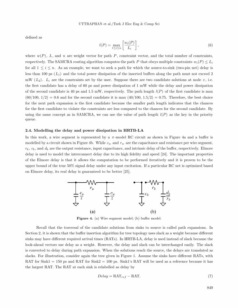
In this work, a wire segment is represented by a π -model RC circuit as shown in Figure 4a and a buffer is

modelled by a circuit shown in Figure 4b. While cw and rw are the capacitance and resistance per wire segment,

rb , cb , and db are the output resistance, input capacitance, and intrinsic delay of the buffer, respectively. Elmore

delay is used to model the interconnect delay due to its high fidelity and speed [24]. The important properties

of the Elmore delay is that it allows the computation to be performed iteratively and it is proven to be the

upper bound of the true 50% signal delay under any input excitation. If a particular RC net is optimized based

on Elmore delay, its real delay is guaranteed to be better [25].

Figure 4. (a) Wire segment model; (b) buffer model.

Recall that the traversal of the candidate solutions from sinks to source is called path expansions. In

Section 2, it is shown that the buffer insertion algorithm for tree topology uses slack as a weight because different

sinks may have different required arrival times (RATs). In HRTB-LA, delay is used instead of slack because the

look-ahead vectors use delay as a weight. However, the delay and slack can be interchanged easily. The slack

is converted to delay during path expansion. When the solutions reach the source, the delays are translated as

slacks. For illustration, consider again the tree given in Figure 1. Assume the sinks have different RATs, with

RAT for Sink1 = 150 ps and RAT for Sink2 = 100 ps. Sink1’s RAT will be used as a reference because it has

the largest RAT. The RAT at each sink is relabelled as delay by

Delay = RATref − RAT. (7)

849

UTTRAPHAN et al./Turk J Elec Eng & Comp Sci

Therefore, Sink1 and Sink2 will have an initial delay of 0 and 50 ps, respectively. At the end of computation,

the delays at the source node are converted back to slacks.

The path expansions in HRTB-LA are based on the path expansion in the S-RABILA algorithm where

the capacitance-delay (c , t) pair is propagated from sinks towards the source. However, in order to handle

power constraint, the power dissipation metric is introduced into the candidate solution. The power is computed

based on the model given in [9] as follows:

P = αCV 2DDf + Pl + Ps. (8)

The first term represents the switching power, where α , C , VDD , and f are the switching factor, total load

capacitance, power supply, and clock frequency, respectively. The second term, Pl is the leakage power and

the last term, Ps is the short circuit power. With faster signal slew rates in subnanometer technologies, the

dominance of the leakage power has increased, and the significance of the short circuit power in total power

dissipation is decreased [9]. As in [9], the short circuit power is not included in our computation.

Hence, the candidate solution for HRTB-LA is a capacitance–delay–power (c , t , p) tuple. Note that one

of the key contributions in this work is to propose the power computation scheme in dynamic programming

framework. In the next section, we will discuss these computation schemes in HRTB-LA. There are two

computation schemes in HRTB-LA. The first scheme is called upstream computation and it is used to compute

the candidate solutions. The second scheme is called downstream computation and it is used to compute the

look-ahead weight vectors.

2.5. Upstream delay and power computation

In this scheme, each node v is labeled with a three-tuple (c , t , p), where c , t , and p represent the capacitance,

delay, and power dissipation from node v to a sink node, respectively. With an initial (c , t , p) tuple, a new

(c ’, t ’, p ’) tuple for the upstream interconnect segment is determined. If the upstream segment is only a wire

segment, the new (c ’, t ’, p ’) is given by

c′ = c+ cw, t′ = rw

(cw2

+ c)+ t and p′ = p. (9)

If the upstream segment is a wire terminated with a buffer, the new (c ’, t ’, p ’) becomes

c′ = cw + cb, t′ = rw

(cw2

+ cb

)+ db + rbc+ t and p′ = p+ α

(dbrb

+ c

)V 2DDf + Pl. (10)

If the solutions from the right child (c , t , p)right and the left child (c , t , p)left meet at a Steiner node, the

branch merging operation is performed as given by

c′ = cright + cleft, t′ = max (tright, tleft) and p′ = pright + pleft. (11)

Finally when the solution reaches the source node, then the total delay is

Delay = cRs + t (12)

and the total power dissipation is

Power = p+ αcV 2DDf. (13)

850

UTTRAPHAN et al./Turk J Elec Eng & Comp Sci

2.6. Downstream delay and power computation

In this scheme, each node u is labeled with a four-tuple (r , t , c , p), where r , t , c , and p are resistance,

delay, capacitance, and power dissipation from source node/Steiner node up to node u , respectively. Given a

(r , t , c , p) tuple at node u , a new tuple for the downstream segment at node v is computed as follows. If the

downstream segment is a wire, then (r ’, t ’, c ’, p ’) is

r′ = rw + r, t′ =(r +

rw2

)cw + t, c′ = c+ cw and p′ = p. (14)

If the segment consists of wire terminated by buffer, then (r ’, t ’, c ’, t ’) is

r′ = rb, t′ = r(cw + cb) + rw

(cw2

+ cb

)+ db + t, c′ =

dbrb

and p′ = p+ α (c+ cw + cb)V2DDf + Pl. (15)

If the solution reaches a sink node, then the total delay is

Delay = rCL + t (16)

and the total power dissipation is

Power = p+ α (c+ cw + CL)V2DDf. (17)

3. Description of HRTB-LA algorithm

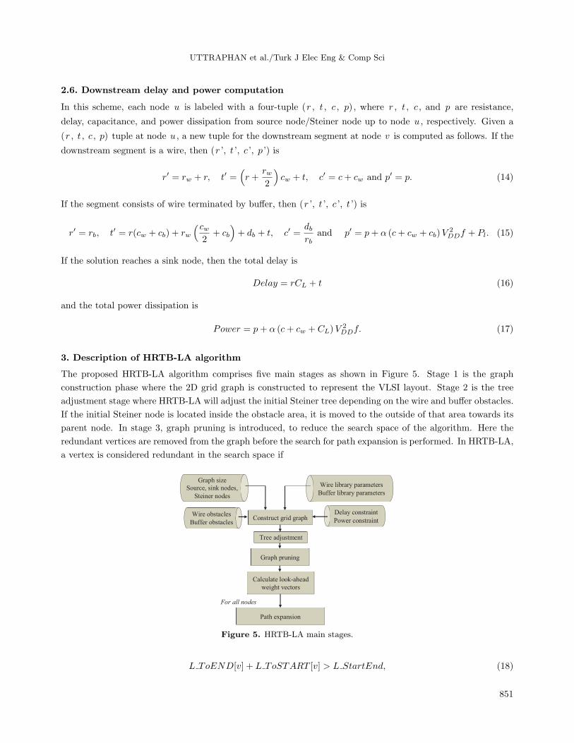
The proposed HRTB-LA algorithm comprises five main stages as shown in Figure 5. Stage 1 is the graph

construction phase where the 2D grid graph is constructed to represent the VLSI layout. Stage 2 is the tree

adjustment stage where HRTB-LA will adjust the initial Steiner tree depending on the wire and buffer obstacles.

If the initial Steiner node is located inside the obstacle area, it is moved to the outside of that area towards its

parent node. In stage 3, graph pruning is introduced, to reduce the search space of the algorithm. Here the

redundant vertices are removed from the graph before the search for path expansion is performed. In HRTB-LA,

a vertex is considered redundant in the search space if

For all nodes

Graph size Source, sink nodes,

Steiner nodes

Wire obstacles Buffer obstacles

Wire library parameters Buffer library parameters

Construct grid graph

Path expansion

Graph pruning

Tree adjustment

Delay constraint Power constraint

Calculate look-ahead

weight vectors

Figure 5. HRTB-LA main stages.

L ToEND[v] + L ToSTART [v] > L StartEnd, (18)

851

UTTRAPHAN et al./Turk J Elec Eng & Comp Sci

where L ToEND [v ] is the shortest length from vertex v to the sink node END while L ToSTART [v ] is the

shortest length from vertex v to the source node START. These paths are computed by ignoring buffer obstacles.

The reference path length L StartEnd is the length of the shortest path from START to END considering buffer

obstacles.

Stage 4 is the look-ahead weight vector calculation and stage 5 is the path expansion stage. The maze

search starts from each sink towards the Steiner node where the branch merging operations are performed to

create a new solution set. These solutions will be propagated toward the source and the best solution is selected

as a final solution. As they are the most critical parts of our proposed algorithm, stages 4 and 5 of the algorithm

are explained in more detail in the following section.

3.1. Path expansion and look-ahead scheme

Figure 6 shows the pseudo-code for the path expansion in HRTB-LA. The path expansion in our algorithm is

implemented using a priority queue. We now explain the path expansion and look-ahead scheme with a simple

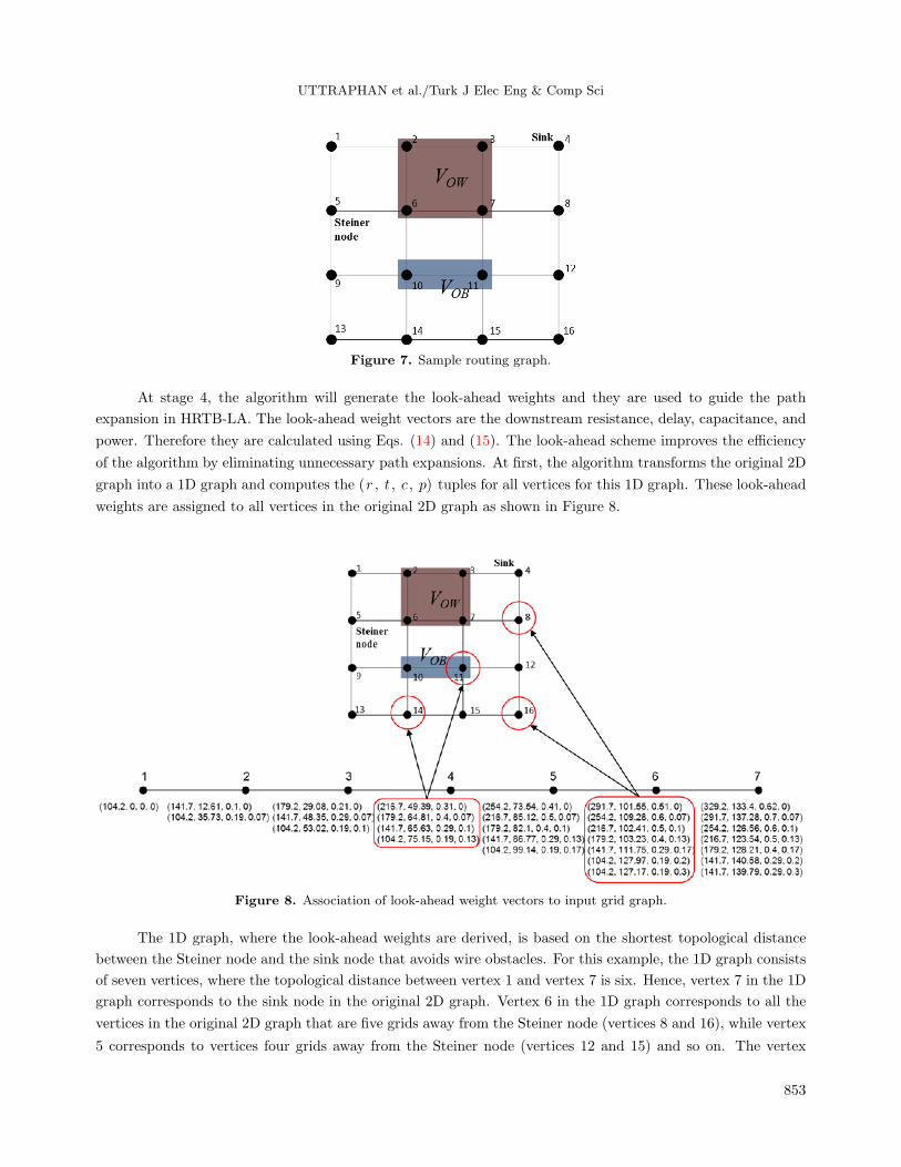
grid graph illustrated in Figure 7. In this example, without loss of generality, the graph only has one sink.

Vertices 4 and 5 are sink node and Steiner node, respectively. Vertices 2, 3, 6, and 7 are wire obstacle vertices

VOW , and vertices 10 and 11 are buffer obstacle vertices VOB . The parameters used for computation are as in

Section 2, with additional parameters switching factor α = 0.15 [9], VDD = 1 V, clock frequency f = 2 GHz,

and leakage power Pl = 0.036 mW.

Figure 6. Pseudo-code of the path expansion in HRTB-LA.

852

UTTRAPHAN et al./Turk J Elec Eng & Comp Sci

Figure 7. Sample routing graph.

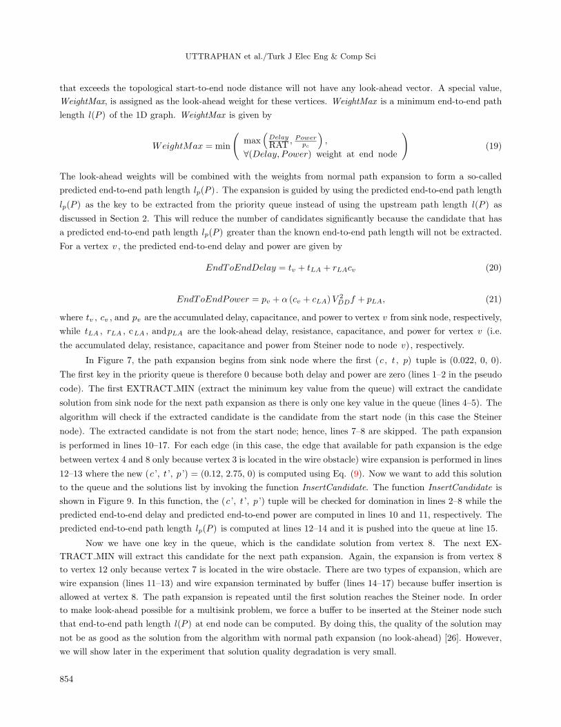
At stage 4, the algorithm will generate the look-ahead weights and they are used to guide the path

expansion in HRTB-LA. The look-ahead weight vectors are the downstream resistance, delay, capacitance, and

power. Therefore they are calculated using Eqs. (14) and (15). The look-ahead scheme improves the efficiency

of the algorithm by eliminating unnecessary path expansions. At first, the algorithm transforms the original 2D

graph into a 1D graph and computes the (r , t , c , p) tuples for all vertices for this 1D graph. These look-ahead

weights are assigned to all vertices in the original 2D graph as shown in Figure 8.

Figure 8. Association of look-ahead weight vectors to input grid graph.

The 1D graph, where the look-ahead weights are derived, is based on the shortest topological distance

between the Steiner node and the sink node that avoids wire obstacles. For this example, the 1D graph consists

of seven vertices, where the topological distance between vertex 1 and vertex 7 is six. Hence, vertex 7 in the 1D

graph corresponds to the sink node in the original 2D graph. Vertex 6 in the 1D graph corresponds to all the

vertices in the original 2D graph that are five grids away from the Steiner node (vertices 8 and 16), while vertex

5 corresponds to vertices four grids away from the Steiner node (vertices 12 and 15) and so on. The vertex

853

UTTRAPHAN et al./Turk J Elec Eng & Comp Sci

that exceeds the topological start-to-end node distance will not have any look-ahead vector. A special value,

WeightMax, is assigned as the look-ahead weight for these vertices. WeightMax is a minimum end-to-end path

length l(P ) of the 1D graph. WeightMax is given by

WeightMax = min

(max

(Delay

RAT , Powerpc

),

∀(Delay, Power) weight at end node

)(19)

The look-ahead weights will be combined with the weights from normal path expansion to form a so-called

predicted end-to-end path length lp(P ). The expansion is guided by using the predicted end-to-end path length

lp(P ) as the key to be extracted from the priority queue instead of using the upstream path length l(P ) as

discussed in Section 2. This will reduce the number of candidates significantly because the candidate that has

a predicted end-to-end path length lp(P ) greater than the known end-to-end path length will not be extracted.

For a vertex v , the predicted end-to-end delay and power are given by

EndToEndDelay = tv + tLA + rLAcv (20)

EndToEndPower = pv + α (cv + cLA)V2DDf + pLA, (21)

where tv , cv , and pv are the accumulated delay, capacitance, and power to vertex v from sink node, respectively,

while tLA , rLA , cLA , andpLA are the look-ahead delay, resistance, capacitance, and power for vertex v (i.e.

the accumulated delay, resistance, capacitance and power from Steiner node to node v), respectively.

In Figure 7, the path expansion begins from sink node where the first (c , t , p) tuple is (0.022, 0, 0).

The first key in the priority queue is therefore 0 because both delay and power are zero (lines 1–2 in the pseudo

code). The first EXTRACT MIN (extract the minimum key value from the queue) will extract the candidate

solution from sink node for the next path expansion as there is only one key value in the queue (lines 4–5). The

algorithm will check if the extracted candidate is the candidate from the start node (in this case the Steiner

node). The extracted candidate is not from the start node; hence, lines 7–8 are skipped. The path expansion

is performed in lines 10–17. For each edge (in this case, the edge that available for path expansion is the edge

between vertex 4 and 8 only because vertex 3 is located in the wire obstacle) wire expansion is performed in lines

12–13 where the new (c ’, t ’, p ’) = (0.12, 2.75, 0) is computed using Eq. (9). Now we want to add this solution

to the queue and the solutions list by invoking the function InsertCandidate. The function InsertCandidate is

shown in Figure 9. In this function, the (c ’, t ’, p ’) tuple will be checked for domination in lines 2–8 while the

predicted end-to-end delay and predicted end-to-end power are computed in lines 10 and 11, respectively. The

predicted end-to-end path length lp(P ) is computed at lines 12–14 and it is pushed into the queue at line 15.

Now we have one key in the queue, which is the candidate solution from vertex 8. The next EX-

TRACT MIN will extract this candidate for the next path expansion. Again, the expansion is from vertex 8

to vertex 12 only because vertex 7 is located in the wire obstacle. There are two types of expansion, which are

wire expansion (lines 11–13) and wire expansion terminated by buffer (lines 14–17) because buffer insertion is

allowed at vertex 8. The path expansion is repeated until the first solution reaches the Steiner node. In order

to make look-ahead possible for a multisink problem, we force a buffer to be inserted at the Steiner node such

that end-to-end path length l(P ) at end node can be computed. By doing this, the quality of the solution may

not be as good as the solution from the algorithm with normal path expansion (no look-ahead) [26]. However,

we will show later in the experiment that solution quality degradation is very small.

854

UTTRAPHAN et al./Turk J Elec Eng & Comp Sci

Figure 9. Pseudo-code of the Insert candidate in HRTB-LA

The path length of the solution that reaches the Steiner node (or source node) is recorded as a known

minimum end-to-end path length l(P ). For the other path expansions, if the predicted end-to-end path length

lp(P ) is greater than the actual known minimum end-to-end path length l(P ), this candidate solution is

considered dominated, and therefore removed. In this way, the number of candidates at the vertices can be

substantially reduced, thus speeding up the routing path construction.

3.2. Time complexity of HRTB-LA

The proposed algorithm uses the Fibonacci heap [27] to implement the priority queue required for its operations.

The advantage of the Fibonacci heap over other heap algorithms such as binary heap and binomial heap is that it

has much faster operations for the INSERT (used to add a new key into the queue) and DECREASE KEY (used

to remove the redundant key from the queue) functions. These two functions are implicitly called in function

InsertCandidate of HRTB-LA. The time complexities for heap operations of the Fibonacci heap compared to

the binary and binomial heaps are shown in the Table.

Table. Time complexity for heap operations for binary, binomial, and Fibonacci heaps.

Operations Binary heap Binomial heap Fibonacci heapCREATE HEAP Θ Θ ΘINSERT Θ (log n) Θ (log n) ΘEXTRACT MIN Θ (log n) Θ (log n) O(log n)DECREASE KEY Θ (log n) Θ (log n) Θ

855

UTTRAPHAN et al./Turk J Elec Eng & Comp Sci

In the HRTB-LA algorithm, the most time consuming part is the path expansion process (Figure 6).

In the function Path Expansion, the number of EXTRACT-MIN operations in the priority queue is upper

bounded by the total number of vertices |V | . Since the Fibonacci heap is used to implement the priority queue,

the amortized time for EXTRACT MIN operation takes O(|B||V |2 log |V |) because the number of candidate

solutions at each vertex is at most |B||V | [14]. In the Fibonacci heap, each INSERT and DECREASE KEY

operation in the queue takes O (1). Hence, a wire expansion (lines 10–13) takes O(|B||V |) times because

the pruning and the path length prediction operation are linear. Note that the edge connection operation is

bounded by O(|E|), where |E| is the total number of edges. Therefore the total computation time for wire

expansions is O(|B||V ||E|). Meanwhile, the second expansion (wire expansion terminated by buffer, in lines

14–17) takes O(|B|2|V ||E|). Therefore the total running time for the HRTB-LA algorithm is O(|M |(|B||V |2

log |V |+ |B||V ||E|+ |B|2|V ||E|)) ≈ O(|M |(|B||V |2 log |V |+ |B||V |2|E|)), where |M | is the total number of

sinks and Steiner nodes. In practice, the numbers of |E| and |V | are small due to the look-ahead scheme and

graph pruning. This is proved by the experimental results presented in the following section.

4. Experimental work and results

The proposed algorithm is implemented in C running on a 2.4 GHz Intel Core i5 PC with 4 GB RAM. The

algorithm was tested on two randomly generated nets on a 100 × 100 grid graph. The first net has 5 sinks

with 15% wire obstacles and 24% buffer obstacles on the graph. The second net has 25 sinks with 10% wire

obstacles and 20% buffer obstacles on the graph. Two types of test were conducted. To check the solution

quality, we compare the solution from HRTB-LA with the solution from the algorithm that performs a normal

path expansion (no look-ahead) in terms of slack, runtime, and the number of candidate solutions versus the

number of buffers in the library. We refer to the algorithm with normal path expansion as HRTB [26]. We

also compare the solution of HRTB-LA with the solution from RIATA and FBI algorithms to prove that the

solution quality of HRTB-LA algorithm is better than that of the RIATA and FBI algorithms. The power

dissipation constraint was not included in this test because RIATA and FBI did not take power dissipation into

consideration. The code for FBI was downloaded from http://dropzone.tamu.edu/∼zhuoli/

GSRC/fast buffer insertion.html. The code for RIATA is not available for download. Therefore, we coded

our version of RIATA based on the descriptions in [5] and [18].

For all simulations, the chosen wire parameters represent typical interconnect wires used in 65 nm

fabrication. The parameters are compiled by the Nanoscale Integration and Modeling Group at Arizona

State University and are available for download from the Predictive Technology Model (PTM) website at

http://www.eas.asu.edu/∼ptm. The buffer library consists of six buffers. The range of driving resistance is

from 265.9 Ω to 295.0 Ω and the input capacitance is from 0.0309 pF to 0.2317 pF. The power model was

verified by comparing the proposed model with the closed-form solution in [9]. The computation on sample nets

proves that the solution of the proposed model is consistent with the closed-form solution.

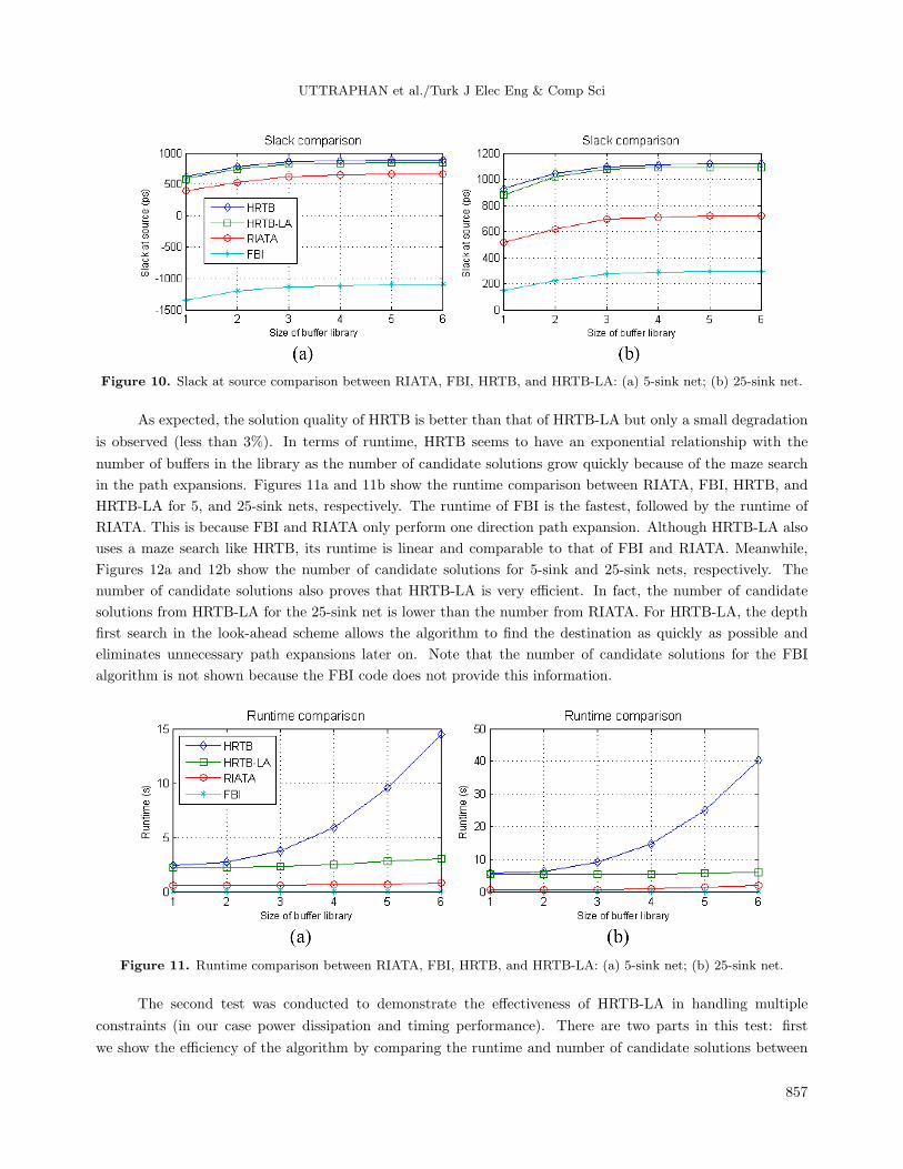
Figures 10a and 10b present the slack at source comparison between RIATA, FBI, HRTB, and HRTB-LA

for 5- and 25-sink nets, respectively. Clearly HRTB and HRTB-LA outperformed RIATA and FBI in both tests

because HRTB and HRTB-LA found the best path for each node by utilizing simultaneous routing and buffer

insertion (maze search). The slack at source for the FBI algorithm does not satisfy the timing constraint in the

test on the 5-sink net. This is because some of the Steiner nodes are located inside the buffer obstacle areas,

which prevents the insertion of buffers on the critical path.

856

UTTRAPHAN et al./Turk J Elec Eng & Comp Sci

Figure 10. Slack at source comparison between RIATA, FBI, HRTB, and HRTB-LA: (a) 5-sink net; (b) 25-sink net.

As expected, the solution quality of HRTB is better than that of HRTB-LA but only a small degradation

is observed (less than 3%). In terms of runtime, HRTB seems to have an exponential relationship with the

number of buffers in the library as the number of candidate solutions grow quickly because of the maze search

in the path expansions. Figures 11a and 11b show the runtime comparison between RIATA, FBI, HRTB, and

HRTB-LA for 5, and 25-sink nets, respectively. The runtime of FBI is the fastest, followed by the runtime of

RIATA. This is because FBI and RIATA only perform one direction path expansion. Although HRTB-LA also

uses a maze search like HRTB, its runtime is linear and comparable to that of FBI and RIATA. Meanwhile,

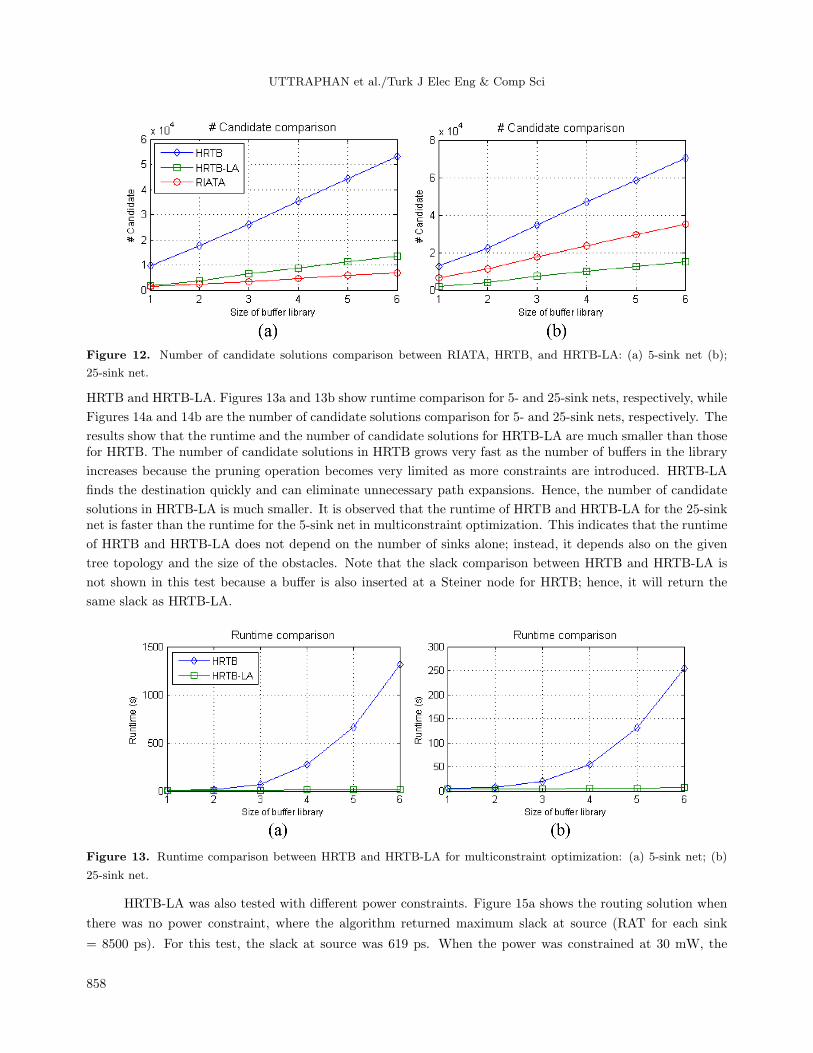
Figures 12a and 12b show the number of candidate solutions for 5-sink and 25-sink nets, respectively. The

number of candidate solutions also proves that HRTB-LA is very efficient. In fact, the number of candidate

solutions from HRTB-LA for the 25-sink net is lower than the number from RIATA. For HRTB-LA, the depth

first search in the look-ahead scheme allows the algorithm to find the destination as quickly as possible and

eliminates unnecessary path expansions later on. Note that the number of candidate solutions for the FBI

algorithm is not shown because the FBI code does not provide this information.

Figure 11. Runtime comparison between RIATA, FBI, HRTB, and HRTB-LA: (a) 5-sink net; (b) 25-sink net.

The second test was conducted to demonstrate the effectiveness of HRTB-LA in handling multiple

constraints (in our case power dissipation and timing performance). There are two parts in this test: first

we show the efficiency of the algorithm by comparing the runtime and number of candidate solutions between

857

UTTRAPHAN et al./Turk J Elec Eng & Comp Sci

Figure 12. Number of candidate solutions comparison between RIATA, HRTB, and HRTB-LA: (a) 5-sink net (b);

25-sink net.

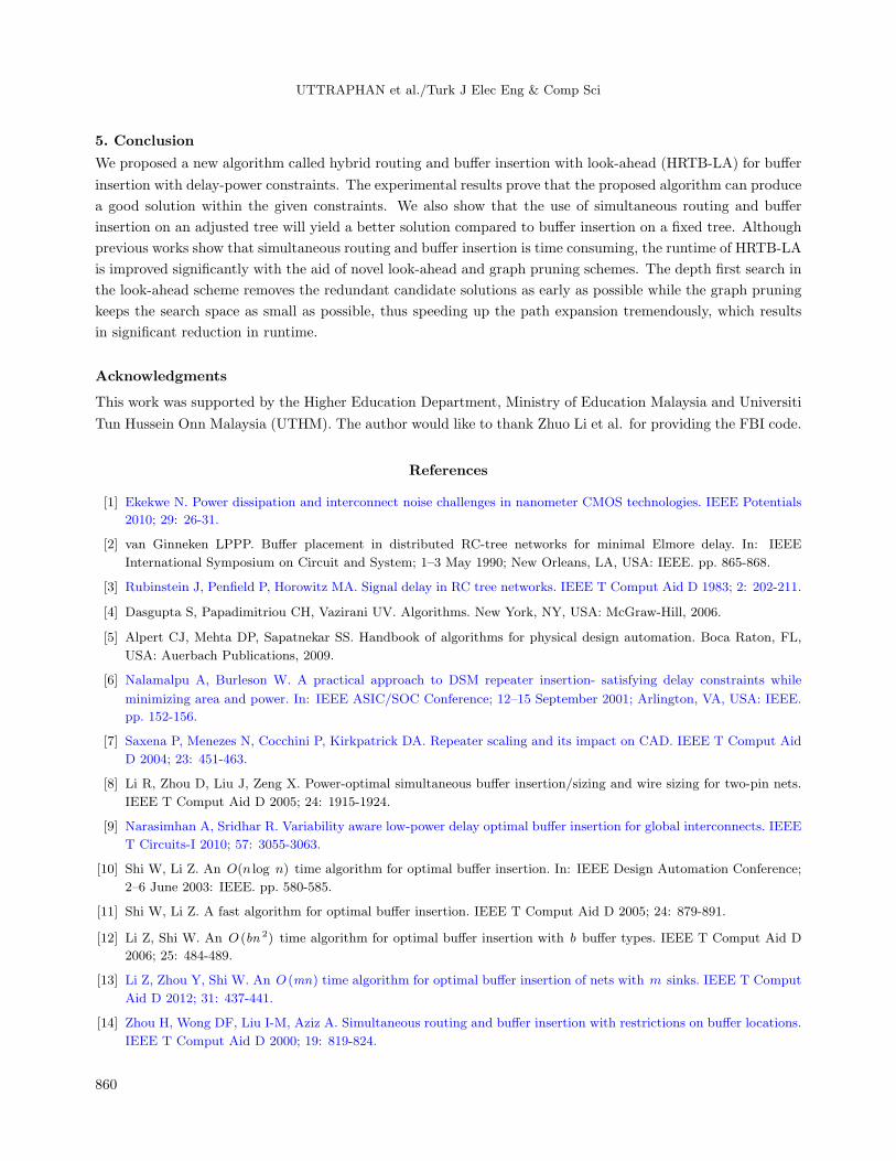
HRTB and HRTB-LA. Figures 13a and 13b show runtime comparison for 5- and 25-sink nets, respectively, while

Figures 14a and 14b are the number of candidate solutions comparison for 5- and 25-sink nets, respectively. The

results show that the runtime and the number of candidate solutions for HRTB-LA are much smaller than thosefor HRTB. The number of candidate solutions in HRTB grows very fast as the number of buffers in the library

increases because the pruning operation becomes very limited as more constraints are introduced. HRTB-LA

finds the destination quickly and can eliminate unnecessary path expansions. Hence, the number of candidate

solutions in HRTB-LA is much smaller. It is observed that the runtime of HRTB and HRTB-LA for the 25-sinknet is faster than the runtime for the 5-sink net in multiconstraint optimization. This indicates that the runtime

of HRTB and HRTB-LA does not depend on the number of sinks alone; instead, it depends also on the given

tree topology and the size of the obstacles. Note that the slack comparison between HRTB and HRTB-LA is

not shown in this test because a buffer is also inserted at a Steiner node for HRTB; hence, it will return the

same slack as HRTB-LA.

Figure 13. Runtime comparison between HRTB and HRTB-LA for multiconstraint optimization: (a) 5-sink net; (b)

25-sink net.

HRTB-LA was also tested with different power constraints. Figure 15a shows the routing solution when

there was no power constraint, where the algorithm returned maximum slack at source (RAT for each sink

= 8500 ps). For this test, the slack at source was 619 ps. When the power was constrained at 30 mW, the

858

UTTRAPHAN et al./Turk J Elec Eng & Comp Sci

algorithm returned a slack at source of 580 ps and power dissipation of 25 mW. The routing solution is given in

Figure 15b. The number of buffers inserted on the net was reduced in order to meet the power constraint, thus

reducing the slack. Figure 15c shows the solution when the power constraint was reduced further to 20 mW.

The algorithm returned a slack at source of 289 ps and power dissipation of 17 mW.

Figure 14. Number of candidate solutions comparison between HRTB and HRTB-LA for multiconstraint optimization:

(a) 5-sink net; (b) 25-sink net.

(a)

(b)

(c)

Figure 15. Routing solutions for 4-sink net for different power constraints: (a) routing solution for maximum slack

with no power constraint; (b) routing solution when power was constrained at 30 mW; (c) routing solution when power

was constrained at 20 mW.

859

UTTRAPHAN et al./Turk J Elec Eng & Comp Sci

5. Conclusion

We proposed a new algorithm called hybrid routing and buffer insertion with look-ahead (HRTB-LA) for buffer

insertion with delay-power constraints. The experimental results prove that the proposed algorithm can produce

a good solution within the given constraints. We also show that the use of simultaneous routing and buffer

insertion on an adjusted tree will yield a better solution compared to buffer insertion on a fixed tree. Although

previous works show that simultaneous routing and buffer insertion is time consuming, the runtime of HRTB-LA

is improved significantly with the aid of novel look-ahead and graph pruning schemes. The depth first search in

the look-ahead scheme removes the redundant candidate solutions as early as possible while the graph pruning

keeps the search space as small as possible, thus speeding up the path expansion tremendously, which results

in significant reduction in runtime.

Acknowledgments

This work was supported by the Higher Education Department, Ministry of Education Malaysia and Universiti

Tun Hussein Onn Malaysia (UTHM). The author would like to thank Zhuo Li et al. for providing the FBI code.

References

[1] Ekekwe N. Power dissipation and interconnect noise challenges in nanometer CMOS technologies. IEEE Potentials

2010; 29: 26-31.

[2] van Ginneken LPPP. Buffer placement in distributed RC-tree networks for minimal Elmore delay. In: IEEE

International Symposium on Circuit and System; 1–3 May 1990; New Orleans, LA, USA: IEEE. pp. 865-868.

[3] Rubinstein J, Penfield P, Horowitz MA. Signal delay in RC tree networks. IEEE T Comput Aid D 1983; 2: 202-211.

[4] Dasgupta S, Papadimitriou CH, Vazirani UV. Algorithms. New York, NY, USA: McGraw-Hill, 2006.

[5] Alpert CJ, Mehta DP, Sapatnekar SS. Handbook of algorithms for physical design automation. Boca Raton, FL,

USA: Auerbach Publications, 2009.

[6] Nalamalpu A, Burleson W. A practical approach to DSM repeater insertion- satisfying delay constraints while

minimizing area and power. In: IEEE ASIC/SOC Conference; 12–15 September 2001; Arlington, VA, USA: IEEE.

pp. 152-156.

[7] Saxena P, Menezes N, Cocchini P, Kirkpatrick DA. Repeater scaling and its impact on CAD. IEEE T Comput Aid

D 2004; 23: 451-463.

[8] Li R, Zhou D, Liu J, Zeng X. Power-optimal simultaneous buffer insertion/sizing and wire sizing for two-pin nets.

IEEE T Comput Aid D 2005; 24: 1915-1924.

[9] Narasimhan A, Sridhar R. Variability aware low-power delay optimal buffer insertion for global interconnects. IEEE

T Circuits-I 2010; 57: 3055-3063.

[10] Shi W, Li Z. An O(n log n) time algorithm for optimal buffer insertion. In: IEEE Design Automation Conference;

2–6 June 2003: IEEE. pp. 580-585.

[11] Shi W, Li Z. A fast algorithm for optimal buffer insertion. IEEE T Comput Aid D 2005; 24: 879-891.

[12] Li Z, Shi W. An O (bn 2) time algorithm for optimal buffer insertion with b buffer types. IEEE T Comput Aid D

2006; 25: 484-489.

[13] Li Z, Zhou Y, Shi W. An O (mn) time algorithm for optimal buffer insertion of nets with m sinks. IEEE T Comput

Aid D 2012; 31: 437-441.

[14] Zhou H, Wong DF, Liu I-M, Aziz A. Simultaneous routing and buffer insertion with restrictions on buffer locations.

IEEE T Comput Aid D 2000; 19: 819-824.

860

UTTRAPHAN et al./Turk J Elec Eng & Comp Sci

[15] Cong J, Yuan X. Routing tree construction under fixed buffer locations. In: Design Automation Conference; 5–9

June 2000; Los Angeles, CA, USA: IEEE. pp. 379-384.

[16] Hu S, Li S, Alpert CJ. A fully polynomial time approximation scheme for timing driven minimum cost buffer

insertion. In: Design Automation Conference; 26–31 July 2009; San Francisco, CA, USA: IEEE. pp. 424-429.

[17] Khalil-Hani M, Shaikh-Husin N. An optimization algorithm based on grid-graphs for minimizing interconnect delay

in VLSI layout design. Malayas J Comput Sci 2009; 22: 19-33.

[18] Hu J, Alpert CJ, Quay ST, Gandham G. Buffer insertion with adaptive blockage avoidance. IEEE T Comput Aid

D 2003; 22: 492-498.

[19] Uttraphan C, Shaikh-Husin N, Khalil-Hani M. An optimization algorithm for simultaneous routing and buffer

insertion with delay-power constraints in VLSI Layout Design. In: International Symposium on Quality Electronic

Design; 3–5 March 2014; Santa Clara, CA, USA: IEEE. pp. 357-364.

[20] Lai M, Wong DF. Maze routing with buffer insertion and wiresizing. IEEE T Comput Aid D 2002; 21: 1205-1209.

[21] Lee CY. An algorithm for path connections and its applications. IEEE T Comput 1961; 10: 346-365.

[22] Md-Yusof Z, Khalil-Hani M, Marsono MN, Shaikh-Husin N. Optimizing multi-constraint VLSI interconnect routing.

In: International Symposium on Integrated Circuits; 14–16 December 2009; Singapore: IEEE. pp 655-658.

[23] van Mieghem P, Kuipers F. Concepts of exact QoS routing algorithms. IEEE Acm T Network 2004; 12: 851-864.

[24] Alpert CJ, Karandikar SK, Li Z, Joon Nam G, Quay ST, Sze CN, Villarrubia PG, Yildiz MC. Techniques for fast

physical synthesis. Proceeding of the IEEE 2007; 95: 573-599.

[25] Gupta R, Tutuianu B, Pileggi LT. The Elmore delay as a bound for RC trees with generalized input signals. IEEE

T Comput Aid D 1997; 16: 95-104.

[26] Uttraphan C, Shaikh-Husin N. Hybrid Routing Tree with Buffer Insertion under Obstacle Constraints. In: Student

Conference on Research and Development; 16–17 December 2013; Kuala Lumpur, Malaysia: IEEE. pp. 411-416.

[27] Cormen TH, Leiserson CE, Rivest RL. Introduction to Algorithms. 3rd ed. Boston, MA, USA: McGraw-Hill, 2009.

861