An Optimal Lower Bound on the Number of

Variables for Graph Identification

Jin-yi Cai∗

Computer Science Dept.Princeton UniversityPrinceton, NJ 08540jyc@princeton.edu

Martin Furer†

Dept. of Computer SciencePenn State University

University Park, PA 16802furer@cs.psu.edu

Neil Immerman‡

Computer Science Dept.University. of Massachusetts

Amherst, MA 01003immerman@cs.umass.edu

Combinatorica, (12:4) (1992), 389-410

Abstract

In this paper we show that Ω(n) variables are needed for first-order logic with count-ing to identify graphs on n vertices. The k-variable language with counting is equivalentto the (k − 1)-dimensional Weisfeiler-Lehman method. We thus settle a long-standingopen problem. Previously it was an open question whether or not 4 variables suffice.Our lower bound remains true over a set of graphs of color class size 4. This contrastssharply with the fact that 3 variables suffice to identify all graphs of color class size 3,and 2 variables suffice to identify almost all graphs. Our lower bound is optimal up tomultiplication by a constant because n variables obviously suffice to identify graphs onn vertices.

1 Introduction

In this paper we show that Ω(n) variables are needed for first-order logic with counting todistinguish a sequence of pairs of graphs Gn and Hn. These graphs have O(n) vertices each,have color class size 4, and admit a linear time canonical labeling algorithm. This contrastssharply with results in [10, 27] where it is shown that two variables suffice to identify alltrees and almost all graphs, and that three variables suffice to identify all graphs of colorclass size 3.

∗Research supported by NSF grant CCR-8709818.†Research supported by NSF grant CCR-8805978 and Pennsylvania State University Research Initiation

grant 428-45.‡Research supported by NSF grants DCR-8603346 and CCR-8806308.

1

Another way to interpret our results is with stable colorings of k-tuples of vertices. Thework of Weisfeiler and Lehman [40, 39] on combinatorial and group theoretic properties ofcolored graphs, has inspired the idea of separating the orbits of the automorphism groupof a graph by coloring k-tuples of vertices. Sometimes, this approach is called, the k-dimensional Weisfeiler-Lehman method (k-dim W-L). In the late seventies and early eighties,this method was developed by many researchers, including Faradzev, Zemlyachenko, Babai,and Mathon. With k = 1, this method gives a linear-time graph isomorphism algorithm thatworks for almost all graphs [10]. Furthermore, the fastest known general graph isomorphismalgorithms make use of this method with k = O(

√n) [11]. It had been conjectured that

this method would provide a polynomial time graph isomorphism test at least for graphs ofbounded valence. (Valence is a synonym for degree.) Our result disposes of such conjectures.

Up until now, most lower bounds in this area were proved using random graphs. Thismethod does not work when counting is included in the language because as mentionedabove, almost all graphs can be identified using only two variables with counting. In ourconstruction we choose graphs Tn, (n = 1, 2, . . .) with O(n) vertices and separator size n(Definition 6.3). Then we deterministically modify Tn producing a pair of non-isomorphicgraphs Gn,Hn, which agree on all properties expressible with n variables. Our lower boundis linear in the separator size of the graphs Tn. This linear lower bound, combined with astraightforward upper bound (Proposition 7.3) allows us to precisely determine how manyvariables are needed to identify many classes of graphs in first-order logic, with or withoutcounting.

This paper is organized as follows: In Section 2 we recount some of the history of theWeisfeiler-Lehman method. In Section 3 we give some background in descriptive complexityand explain the significance of this problem from the logical point of view. In Section 4 weintroduce some combinatorial games and prove that they characterize logical equivalencein the languages we are considering. In Section 5 we prove the equivalence of the (k −1)-dimensional Weisfeiler-Lehman method and the k-variable language with counting. InSection 6 we use the above combinatorial game to prove the linear lower bound. Section 7describes some corollaries and extensions of this work.

2 History of the Weisfeiler-Lehman Method

An old basic idea in graph isomorphism testing and canonical labeling is the naive vertexclassification algorithm as described in Read and Corneil [37]. First, the vertices are labeledor colored with their valences. During the iteration, all labels are extended by the multiset(“set” with possibly multiple elements) of the labels of their neighbors. Between rounds, thelabels are replaced by their order numbers in the lexicographic order of all the occurringlabels. This always keeps the labels short. The algorithm stops when the set of labelsstabilizes, meaning that no new differences between vertices are discovered. A labelingalgorithm identifies a class of graphs, if all vertex properties which are invariant underisomorphisms are discovered. In other words, the sets of vertices with the same labels arethe orbits of the automorphism group.

The naive vertex classification algorithm, which we want to call the one dimensional Weisfeiler-Lehman method (1-dim W-L), does not solve the worst cases of the graph isomorphismproblem. Nevertheless, it is usually a good start, and in fact it succeeds most of the time.

2

Babai, Erdos and Selkow [8] have shown that the 1-dim W-L algorithm already producesnormal forms for all but an n−1/7 fraction of the n-vertex graphs. This has been improved toa c−n log n/ log log n fraction [10] producing an average linear time canonical labeling algorithmby handling the few exceptions with a slow algorithm.

Vertex classification is probably the basis of every practical implementation of a graphisomorphism test. For example, this is the case for the “nauty” package [35], which is saidto be the fastest practical graph isomorphism package. It should be mentioned, however,that in addition to vertex refinement, “nauty” makes extensive use of partial automorphisminformation in its backtrack process; and it is not clear whether or not our examples maylead to graphs on which “nauty” requires excessive time. In general, it is quite difficult toconstruct “hard cases” for graph isomorphism.

There is a class of graphs for which the vertex classification algorithm alone is obviouslyuseless, because the algorithm cannot even get started. These are the regular graphs, whichhave the same degree in each vertex. Here it seems quite natural to go beyond vertexclassification to the 2-dim W-L or edge classification algorithm. Initially every ordered pair(u, v) is labeled or colored with one of three possible colors, depending on whether u = vand whether there is an edge u, v. Then information about the multiset of pairs of colorsassigned to paths of length 2 from u to v is repeatedly added to the color of (u, v). Thealgorithm stops when no color class is split any more. A modification of this algorithm hasbeen shown to produce normal forms for all regular graphs in linear average time [29].

The k-tuple coloring algorithm (named k-dim W-L by Babai [13]) classifies k-tuples ofvertices. It might color vertices and edges implicitly by using k-tuples with repetition ofcomponents. It could start with some encoding of the graph into the labels assigned to thek-tuples. For example, the initial label or color of every k-tuple could be the number ofits distinct components except when this number is two. Then two colors could be usedto encode the presence or absence of an edge between the two vertices. We prefer to get aquicker start by initially coloring each k-tuple with its isomorphism type. Repeatedly, thecolor of (u1, . . . , uk) is refined by the n element multiset (containing one element for eachvertex v) of k-tuples of colors previously assigned to

(v, u2, . . . , uk), (u1, v, u3, . . . , uk), . . . , (u1, . . . , uk−1, v)

We only need to consider k-tuples of distinct elements, if we finally color the vertices by themultiset of colors of incident k-tuples. A more formal description of the k-dim W-L methodis given in Section 5.

Possibly weaker algorithms have been considered. We might call them special k-dim W-L algorithms. In Weisfeiler’s book [39] only such a method is mentioned and called deepstabilization. It consists of individualization followed by a low dimensional (k = 1 or 2) W-Lalgorithm. For every distinguished (i.e., initially colored with unique colors) (k − 1)-tupleor (k− 2)-tuple, a 1-dim W-L or a 2-dim W-L respectively is performed to detect invariantproperties of vertices or edges. These methods seem to be weaker than the standard k-dimW-L method.

Two of the current authors have independently reinvented the k-dim W-L algorithm in theearly eighties and conjectured its capability of identifying the graphs of bounded valence(with k being a suitable function of the valence). Later, we have learned that such con-jectures have been around before in the Soviet Union, where the k-dim W-L algorithm (or

3

maybe sometimes a special k-dim W-L algorithm) has been investigated for two decades.Significant results have been obtained by Faradzev’s group, which contributed many papersto Weisfeiler’s book [39]. The Russians have built a huge algebraic theory with extensiveapplications around the notion of stable colorings of pairs. The key notion is that of a cellu-lar algebra (see [39, 30]), which has been discovered in another context and called coherentconfiguration by Higman [21].

Weisfeiler and Lehman have asked whether the special k-dim W-L method with a slowlygrowing value of k would be sufficient to solve the graph isomorphism problem. There wasactually good reason to conjecture k = O(log n) or even O(1) to be sufficient.

The second hope was partly based on the following result of Cameron [14], obtained in-dependently by Gol’fand (cf. [19, 31]). Let us call a graph k-regular, if the number ofcommon neighbors of a k element subset of vertices only depends on the isomorphism typeof the subgraph induced by the k vertices. (1-regular and 2-regular graphs are well knownas regular and strongly regular graphs respectively.) Cameron and Gol’fand have shownthat apart from the pentagon and the line graph of K(3,3), only the trivial examples of5-regular graphs exist, namely the disjoint unions of complete graphs of equal size, andtheir complements (complete multipartite graphs). These graphs are homogeneous, i.e., allisomorphisms of their subgraphs extend to automorphisms. Therefore, they are immune tok-dim W-L refinements for any k: No refinement beyond the isomorphism type of k-tupleswill follow. However, for any other graph, the Cameron-Gol’fand result assures us that the5-dim W-L method will give at least some nontrivial partitioning of the 5-tuples.

Lipton [32] has proved that a special k-dim W-L method with a fixed k is sufficient forcanonical labeling of trivalent (degree 3) graphs with arc-transitive automorphism groups.(An arc is an ordered pair of adjacent vertices.)

Support for the k = O(log n) conjecture has been provided by Gary Miller [36]. He hasshown that for certain classes of strongly regular graphs and other combinatorial objectssuch as Latin squares k = log n is sufficient. Previously, such graphs have been consideredto be difficult examples for isomorphism testing, because of their high degree of regularityand symmetry. The importance of symmetries for graph isomorphism testing has beenpointed out by Babai and by Mathon [34] who showed that the graph isomorphism problemis equivalent to computing the order of automorphism groups of graphs.

Individualization followed by a low (1 or 2) dimensional refinement (i.e., the special W-Lmethod) has produced pioneer results in the areas of bounded valence as well as generalgraph isomorphism and canonical labeling. Babai’s technical report [3] started to use grouptheoretical algorithms to obtain provable upper bounds for isomorphism problems. Notonly did he get his well known probabilistic polynomial time isomorphism test for graphs ofbounded color class size, he also started the work on bounded valence graphs. Individual-ization of k =

√n(log n)c vertices splits a bounded valence graph into color classes of size at

most√n resulting in an exp(

√n(log n)c) isomorphism test. Subsequently Luks [33] proved,

using group theory to greater depth, that isomorphism for graphs of bounded valence is inpolynomial time. Finally the canonical labeling problem for graphs of bounded valence hasbeen solved in polynomial time by [11] and [18] independently.

Individualization followed by naive refinement has also been the tool used by Babai tohandle strongly regular graphs [4] and primitive coherent configurations [6]. He used in-dividualization of k = 2

√n log n vertices. Strongly regular graphs and more generally,

4

coherent configurations are stable under 2-dim W-L. While strongly regular graphs are justundirected graphs, coherent configurations are edge-colored complete directed graphs. Acoherent configuration is primitive if the diagonal has one color and all other colors defineconnected graphs. If a transitive automorphism group is primitive, then 2-dim W-L pro-duces necessarily a primitive coherent configuration. For tournaments, the isomorphismproblems of primitive and arbitrary coherent configurations are polynomial time equivalent[11].

The general graph isomorphism problem has been attacked by Zemlyachenko. The methodis described in [5] and [41]. By individualization of O(

√n) vertices and canonical edge-

switching, he has been able to reduce the valence to O(√n). Combining this with the

method of Luks [33], Zemlyachenko obtained the first interesting upper bound for generalgraph isomorphism [41] (cf. [5]). His bound is exp(n1−c) for some positive constant c. Thishas subsequently been improved by Babai and Luks [11] to exp(n1/2+o(1)).

Instead of measuring the reduction in the valence, one could ask about the effect of thesemethods on the color class size. Babai [7] has investigated this splitting power of Zemly-achenko’s method combined with 2-dim W-L. The result is that individualizing k = O(n2/3 log n)vertices, and applying Zemlyachenko’s method and the 2-dim W-L method, he obtains colorclasses which have ≤ k vertices in each connected component of the resulting graph.

3 Logical Background

In [23, 24, 25] one of us has pursued an alternate view of complexity theory in whichthe complexity of a problem is characterized in terms of the complexity of the simplestfirst-order sentences expressing the problem. For example, it is shown in [23] that thepolynomial-time properties are exactly the properties expressible by first-order sentencesiterated1 polynomially many times:

Fact 3.1 ([23])

P =∞⋃

k=1

FO(≤)[nk]

The notation FO(≤)[nk] denotes the set of properties describable by a very uniform sequenceof sentences ϕn such that each sentence ϕn has length O(nk) and has a bounded numberof variables independent of n.2 The symbol ≤ is included to emphasize the presence of atotal ordering on the universe of the input structures. In [24] and in [38] it is also shownthat this uniform sequence of formulas can be represented by a least fixed point operator(LFP) applied to a single formula. Thus,

P = FO(≤) + LFP =∞⋃

k=1

FO(≤)[nk] .

1More precisely, the sentence expressing the property for structures of size n consists of a fixed block ofrestricted quantifiers written p(n) times, followed by a fixed formula.

2In [23] the notation Var&Sz[O(1), nk] instead of FO[nk] was used.

5

Fact 3.1 gives a natural language expressing exactly the polynomial-time properties of or-dered graphs. Let a graph property be an order independent property of ordered graphs.One can ask the question,

Question 3.2 Is there a natural language for the polynomial-time graph properties?

Since the notion of “natural” is not well defined, some readers may prefer the more precisequestion:

Question 3.3 Is there a recursively enumerable listing of a set of Turing machines thataccept exactly all the polynomial-time graph properties?

These questions were first asked with respect to database query languages [15]. See [28] fora discussion of the role of ordering in the database context.

We remark that should it be the case that graph canonization (i.e. given a graph returna canonical form such that two graphs are isomorphic iff their canonical forms are equal)is in polynomial time, then the answer to Question 3.3 is, “Yes.” Thus a negative answerwould imply that P is not equal to NP.

Previous to this paper, the only polynomial-time graph properties known not to be express-ible in FO + LFP (without ordering) were “counting problems”. For example, that a graphhas an even number of edges is not expressible in FO + LFP. In [24] a language which wenow call “FO+LFP+COUNT” was proposed as an answer to Question 3.2. This languagedescribes two sorted structures consisting of an unordered domain of vertices together withan edge predicate, plus an ordered domain of numbers. The domains are defined via count-ing quantifiers as in Section 3.2. We show in Corollary 7.1 that this language fails badly oncertain linear time properties of graphs.

In [27] and [26] the exact number of variables needed to identify various classes of trees withand without counting, respectively, is determined. (Without counting this number increaseslinearly with the arity of the trees; with counting two variables suffice.) The question ofhow many variables are needed to identify various classes of graphs is interesting in its ownright, and also has applications to temporal logic [26].

In the remainder of this section we explain the logical background we need. Some of thismaterial is described in more detail in [27].

3.1 First-Order Logic

For our purposes, a graph will be defined as a finite first-order structure, G = 〈VG, EG〉. VG

is the universe, (the vertices). EG is a binary relation on VG, (the edges).

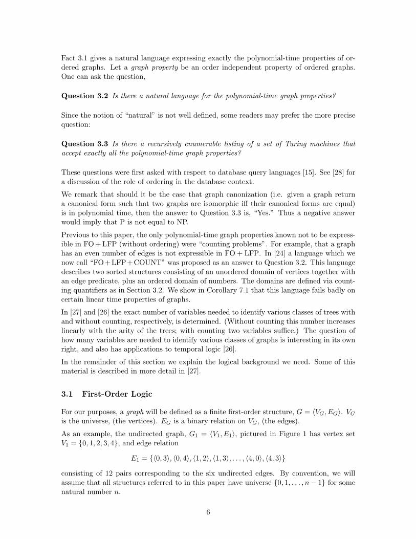
As an example, the undirected graph, G1 = 〈V1, E1〉, pictured in Figure 1 has vertex setV1 = 0, 1, 2, 3, 4, and edge relation

E1 = 〈0, 3〉, 〈0, 4〉, 〈1, 2〉, 〈1, 3〉, . . . , 〈4, 0〉, 〈4, 3〉

consisting of 12 pairs corresponding to the six undirected edges. By convention, we willassume that all structures referred to in this paper have universe 0, 1, . . . , n− 1 for somenatural number n.

6

@@

@

@@

@

•4

•1

•3

•

2•

0

Figure 1: An Undirected Graph

The first-order language of graph theory is built up in the usual way from the variablesx1, x2, . . ., the relations symbols E and =, the logical connectives ∧,∨,¬,→, and the quan-tifiers ∀ and ∃. The quantifiers range over the vertices of the graph in question. For exampleconsider the following first-order sentence:

ϕ ≡ ∀x∀y[E(x, y) → E(y, x) ∧ x 6= y]

ϕ says that G is undirected and loop free. We will only consider graphs that satisfy ϕ, insymbols: G |= ϕ.

It is useful to consider a slightly more general set of structures. The first-order language ofcolored graphs results from the addition of a countable set of unary relations C1, C2, . . .to the first-order language of graphs.3 Define a colored graph to be a graph that interpretsthese new unary relations so that all but finitely many of the predicates are false at eachvertex. These unary relations may be thought of as colorings of the vertices.

Definition 3.4 For a given language L we say that the graphs G and H are L-equivalent(G ≡L H) iff for all sentences ϕ ∈ L,

G |= ϕ ⇔ H |= ϕ .

We say that L identifies the graph G iff for all graphs H, if G ≡L H then G and H areisomorphic. L identifies a set of graphs S if it identifies every element of S.

Note: For the languages Lk, Ck which we consider in this paper, and any graph G, theset of sentences in the language that are true about G has a polynomial size descriptionwhich may be computed in polynomial-time [27]. Thus any set of graphs identified by Lk

or Ck has a polynomial-time canonization algorithm.

Of course the First-Order Language of Colored Graphs identifies all colored graphs. Froma computational viewpoint it is interesting to consider weaker languages admitting muchfaster equivalence testing algorithms.

3.2 The Languages Lk and Ck

Define Lk to be the set of first-order formulas ϕ, such that the variables in ϕ are a subsetof x1, x2, . . . , xk. Note that variables in first-order formulas are similar to variables inprograms: they can be reused (i.e. requantified).

3Coloring relations are a clean tool for restricting the automorphisms of graphs. However, all the coloringrelations in this paper could be replaced by simple gadgets in the graphs, without changing any of the results.

7

For example, consider the following sentence in L2.

ψ ≡ ∀x1∃x2

(E(x1, x2) ∧ ∃x1[¬E(x1, x2)]

)The sentence, ψ, says that every vertex is adjacent to some vertex which is itself notadjacent to every vertex. As an example, the graph from Figure 1 satisfies ψ. Note thatthe outermost quantifier, ∀x1, refers only to the free occurrence of x1 within its scope.

Define a color class to be the set of vertices which satisfy a particular set of color relations.The color class size of a graph is the cardinality of its largest color class. In [27] it is shownthat L3 identifies the set of graphs of color class size 3.

As noted above, the languages Lk are too weak to count, or even to express the parity ofthe number of edges. It is thus natural to strengthen these languages by adding countingquantifiers to the languages Lk, thus obtaining the new languages Ck. For each positiveinteger i, we include the quantifier, (∃i x). The meaning of “(∃17x1)ϕ(x1)”, for example,is that there exist at least 17 vertices such that ϕ. It is sometimes convenient to use thefollowing abbreviation (∃!i x), meaning that there exists exactly i x’s:

(∃!i x)ϕ(x) ≡ (∃i x)ϕ(x) ∧ ¬(∃i+ 1x)ϕ(x)

As an example, the following sentence in C2 says that there exist exactly 17 vertices ofdegree 5,

(∃!17x1)(∃!5x2)E(x1, x2)

As an even worse example, the following sentence in C2 identifies the graph in Figure 1. Itsays that the whole graph contains exactly 5 vertices and that one vertex is adjacent to fourvertices each of which has degree 2.

[(∃!5x1)(x1 = x1)] ∧ [(∃!1x1)(∃4x2)(E(x1, x2) ∧ (∃!2x1)E(x2, x1))]

Note that every sentence in Ck is equivalent to an ordinary first-order sentence with perhapsmany more variables and quantifiers. In Section 5 it is shown that testing Ck equivalencecorresponds to the (k− 1)-dimensional Weisfeiler-Lehman Method. It thus follows that thelanguage C2 identifies all trees and almost all graphs. In [27], TIME(nk log n) algorithmsfor testing Lk or Ck equivalence of graphs on n vertices are presented.

4 Pebbling Games

We next describe two pebbling games that are equivalent to testing Lk and Ck equivalence,respectively. These games are variants of the games of Ehrenfeucht and Fraısse, [16, 17].The results in this section concerning the Lk game and the Ck game originally appeared in[23] and [27], respectively.

Let G and H be two graphs, and let m and k be natural numbers. Define the m-move Lk

game on G and H as follows. There are two players, and for each variable xi, i = 1, . . . , kthere is a pair of xi pebbles.

8

On each move, Player I picks up the pair of xi pebbles, for some i ∈ 1, . . . , k, and heplaces one of them on a vertex in one of the graphs.4 Player II must then place the otherxi pebble on a vertex of the other graph.

Define a k-configuration on a pair of graphs G,H to be a pair (u, v) of partial functions,

u : x1, . . . , xk → VG; v : x1, . . . , xk → VH

such that the domains of u and v are equal. We will use the notation Du to denote thedomain of the partial function u. Thus a k-configuration on G,H is a valid position of theLk game on G,H. Here u(xi) = g means that an xi pebble is on g ∈ VG. If xi 6∈ Du = Dv

this means that the xi pebbles are not currently placed on the board.

Let (ur, vr) be the configuration of the game after move number r. Then we say PlayerI wins the game after move r if the map that takes ur(xi) to vr(xi), i ∈ Dur , is not anisomorphism of the subgraphs induced by these vertices. (Note that if the graphs arecolored then an isomorphism must preserve colors as well as edges.) We say that Player Iwins the m-move game if for some r ∈ 0, 1, 2, . . . ,m, Player I wins the game after mover. Player II wins iff Player I does not win. Finally, we say that Player II has a winningstrategy for the Lk game on G and H, iff for all m, Player II has a winning strategy for them-move game on G and H.

Thus Player II has a winning strategy for the Lk game just if she can always find matchingvertices to preserve the isomorphism.5 Player I is trying to point out a difference betweenthe two graphs and Player II is trying to keep them looking the same.

The number of moves in the Lk game corresponds to the depth of nesting of quantifiers ofthe sentences in Lk needed to distinguish the graphs G and H. Define the language Lk,m

to be the restriction of Lk to formulas of quantifier depth m. The relationship between theLk game and the language Lk is given in Theorem 4.2. Before we state it, we need thefollowing definition.

Definition 4.1 Let G,H be a pair of graphs and let (u, v) be a k-configuration on G,H.We will say that G is Lk,m-equivalent to H, in symbols, G ≡Lk,m

H iff for all formulasϕ ∈ Lk,m whose free variables are a subset of Du,

G, u |= ϕ ⇔ H, v |= ϕ

Similarly we will say that G is Lk-equivalent to H, in symbols, G ≡LkH iff for all m,

G ≡Lk,mH.

Theorem 4.2 ([23]) Player II has a winning strategy for the m-move Lk game on G,Hif and only if G ≡Lk,m

H. Thus, Player II has a winning strategy for the Lk game on G,Hiff G ≡Lk

H.

Before we prove Theorem 4.2, we will give a few examples of the game.4To make the play of the games easier to follow we will use masculine pronouns for Player I and feminine

pronouns for Player II.5By definition, the strategy can depend on the given number m of moves, but as G and H are finite,

there is actually one strategy winning for all m.

9

G H

•b

•r

•y

@@@

•b

•r

•y

@@@

•y

•b

•r@

@@•y

•b

•r@

@@

Figure 2: The L2 Game

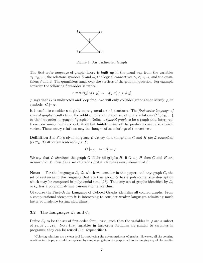
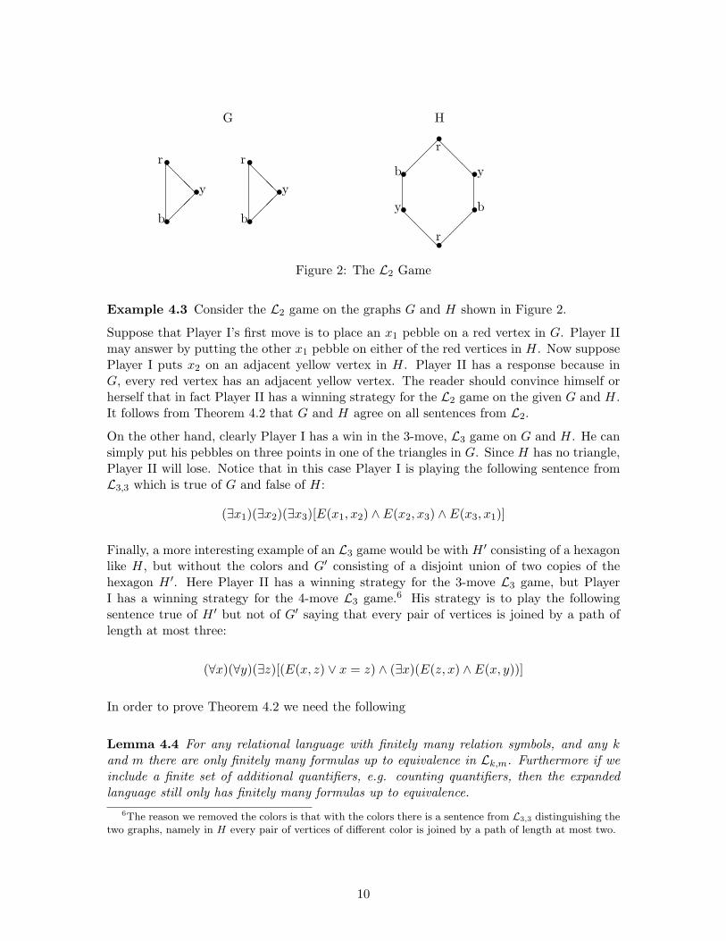
Example 4.3 Consider the L2 game on the graphs G and H shown in Figure 2.

Suppose that Player I’s first move is to place an x1 pebble on a red vertex in G. Player IImay answer by putting the other x1 pebble on either of the red vertices in H. Now supposePlayer I puts x2 on an adjacent yellow vertex in H. Player II has a response because inG, every red vertex has an adjacent yellow vertex. The reader should convince himself orherself that in fact Player II has a winning strategy for the L2 game on the given G and H.It follows from Theorem 4.2 that G and H agree on all sentences from L2.

On the other hand, clearly Player I has a win in the 3-move, L3 game on G and H. He cansimply put his pebbles on three points in one of the triangles in G. Since H has no triangle,Player II will lose. Notice that in this case Player I is playing the following sentence fromL3,3 which is true of G and false of H:

(∃x1)(∃x2)(∃x3)[E(x1, x2) ∧ E(x2, x3) ∧ E(x3, x1)]

Finally, a more interesting example of an L3 game would be with H ′ consisting of a hexagonlike H, but without the colors and G′ consisting of a disjoint union of two copies of thehexagon H ′. Here Player II has a winning strategy for the 3-move L3 game, but PlayerI has a winning strategy for the 4-move L3 game.6 His strategy is to play the followingsentence true of H ′ but not of G′ saying that every pair of vertices is joined by a path oflength at most three:

(∀x)(∀y)(∃z)[(E(x, z) ∨ x = z) ∧ (∃x)(E(z, x) ∧ E(x, y))]

In order to prove Theorem 4.2 we need the following

Lemma 4.4 For any relational language with finitely many relation symbols, and any kand m there are only finitely many formulas up to equivalence in Lk,m. Furthermore if weinclude a finite set of additional quantifiers, e.g. counting quantifiers, then the expandedlanguage still only has finitely many formulas up to equivalence.

6The reason we removed the colors is that with the colors there is a sentence from L3,3 distinguishing thetwo graphs, namely in H every pair of vertices of different color is joined by a path of length at most two.

10

Proof This is easy to see by induction on m. When m = 0, there are only finitely manyvariables and only finitely many relation symbols, so only finitely many sets of possiblefacts about these variables. Assume that there are a total of f different kinds of quantifiers.Inductively, assume there are sm inequivalent formulas of quantifier depth m. Then thereare no more than 22fksm inequivalent formulas of quantifier depth m+ 1.

Proof of Theorem 4.2: We prove by induction on m, that for all k-configurations (u, v)on G,H the following statements are equivalent:

1. Player II has a winning strategy for the m-move Lk game on G,H starting from theinitial configuration (u, v).

2. G, u ≡Lk,mH, v

The base of the induction is immediate because the map from u(Du) to v(Du) is an isomor-phism of the induced subgraphs iff G, u and H, v agree on all quantifier-free formulas.7

Assume the equivalence of (1) and (2) for all m-move games, and let (u, v) be the initialconfiguration of an (m+1)-move game. Assume condition (2) is false and let ϕ ∈ Lk,m+1 bea formula on which G, u and H, v disagree. If ϕ is a disjunction, conjunction, or negation ofsmaller formulas then G, u and H, v must disagree on one of these smaller formulas, so wemay assume that ϕ begins with a quantifier. We may assume by symmetry that ϕ = (∃xi)ψand G, u |= ϕ, but H, v |= ¬ϕ. Player I should then place one of the xi pebbles on a vertex gsuch that ψ holds in G, u(xi/g). No matter what vertex h Player II answers with, we knowthat ¬ψ will hold in H, v(xi/h). Letting (u1, v1) = (u(xi/g), v(xi/h)) be the configurationafter this move we have that G, u1 6≡k,m H, v1. Thus by induction Player I has a winningstrategy for the remaining m-move game and thus for the original m+ 1-move game.

Conversely, assume that condition (2) is true and let Player I’s first move be to place one ofthe xi pebbles on some vertex g from G. Let u1 = u(xi/g) be the result of this move. Notethat there are only finitely many color predicates that any vertex in G or H satisfies. Thus,Lemma 4.4 applies and there is only a finite set Fk,m of inequivalent formulas of interest inLk,m. Define S to be the set of formulas in Fk,m that are satisfied by G, u1 and let σ be theconjunction of the finitely many formulas in S. Thus we have that

G, u |= (∃xi)σ

It follows that H, v |= (∃xi)σ. Let Player II place the other xi pebble on a witness, h, for σin H, and let v1 = v(xi/h) be the result of this move. By the definition of σ it follows that

G, u1 ≡Lk,mH, v1

Thus it follows by induction that Player II has a winning strategy for the remaining m-movegame and thus also for the original m+ 1-move game.

7We are presenting the proof here for the language with no constant or function symbols. The proof goesthrough when function symbols are present, under the additional assumption that the cardinality of anyfinitely generated set is finite [26].

11

4.1 The Ck Game

A modification of the Lk game provides a combinatorial tool for analyzing the expressivepower of Ck. Given a pair of graphs define the Ck game on G and H as follows: Just as inthe Lk game, we have two players and k pairs of pebbles. The difference is that each movenow has two parts.

1. Player I picks up the xi pebble pair for some i. He then chooses a set A of verticesfrom one of the graphs. Now Player II answers with a set B of vertices from the othergraph. B must have the same cardinality as A.

2. Player I places one of the xi pebbles on some vertex b ∈ B. Player II answers byplacing the other xi pebble on some a ∈ A.

The definition for winning is as before. What is going on in the two part move is that PlayerI asserts that there exist |A| vertices in G with a certain property. Player II answers withthe same number of such vertices in H. Player I challenges one of the vertices in B andPlayer II replies with an equivalent vertex from A. This game captures expressibility in Ck:

Theorem 4.5 ([27]) Player II has a winning strategy for the Ck game on G,H if and onlyif G ≡Ck

H.

Theorem 4.5 follows from Theorem 5.2, which we prove in the next section.

5 Ck-Equivalence Equals (k − 1)-dim W-L

In this section we describe the k-dimensional Weisfeiler-Lehman method (k-dim W-L). Wethen prove that a pair of k-tuples of vertices from a graph agree on all formulas in Ck+1 iffthey are in the same equivalence class arising from the k-dim W-L.

The 1-dim W-L is also called vertex refinement. Let G = 〈V,E,C1, . . . , Cr〉 be a coloredgraph in which every vertex satisfies exactly one color relation. Let W 0 : V → 1 . . . n begiven by W 0(v) = i iff v ∈ Ci. We then define W r+1, the refinement of W r as follows: Thenew color of each vertex g is defined to be the following tuple:

〈W r(g), y1, n1, . . . , yr, nr〉

where yi is the number of vertices of color i that g is adjacent to, and ni is the number ofvertices of color i that g is not adjacent to. In practice, we sort these new colors lexico-graphically and assign W r+1(g) to be the number of the new color class that g inhabits.However, we retain a table decoding the “meaning” of each of the colors. Thus two verticesare in the same new color class precisely if they were in the same old color class, and theywere adjacent to the same number of vertices of each color. We keep refining the coloringuntil at some level W r = W r+1. We let W = W r and call W the stable refinement of W 0.

We will see in Theorem 5.2 that stable coloring provides exactly the same information asC2 equivalence.

12

Next define the k-dim W-L for k > 1 as follows. Let G be a colored graph and let u bea (total) map from x1, . . . , xk to VG. Define the initial color W 0(u) according to theisomorphism type of u. That is, W 0(u) = W 0(v) iff the map from (u(x1), . . . , u(xk)) to(v(x1), . . . , v(xk)) is an isomorphism.

For each g ∈ VG, define the operation

sift(f, u, g) = 〈f(u(x1/g)), f(u(x2/g)), . . . , f(u(xk/g))〉

Thus sift(W r, u, g) is the k-tuple of W r-colors arising from substituting g in turn for eachof the k positions in u.

We define the r+ 1st color of u from the rth color by considering the rth color of u togetherwith the number of vertices g such that sift(W r, u, g) = t for each possible k-tuple of colorst. More explicitly, form the new color of u as the tuple:

〈W r(u),SORTsift(W r, u, g) | g ∈ G〉

As in the one dimensional case, we sort these new colors lexicographically, and assignW r+1 according to the ordering that ensues. However, we do retain a table decodingthe meaning of each color. Thus for a pair of configurations u, v from different graphs,W r+1(u) = W r+1(v) iff the numbers of the colors assigned are the same, and the decodingtables for the two graphs are identical. Thus W r+1(u) = W r+1(v) just if W r(u) = W r(v)and for each k-tuple of colors t,

|g | sift(W r, u, g) = t| = |g | sift(W r, v, g) = t| (5.1)

(Note that the difference between the case k = 1 and the case k > 1 is that in the formercase we have to explicitly consider which of the g’s are adjacent to u(x1) in the abovedefinition of new color; whereas, for k > 1, this adjacency is part of the information in theinitial color of the tuples u(xj/g) for j 6= 1.)

Let W (u) denote the stable color of u. Note that there can be at most nk color classes fora graph with n vertices and thus the algorithm stops after at most nk iterations.

Theorem 5.2 Let G,H be a pair of colored graphs and let (u, v) be a k-configuration onG,H, where k ≥ 1. Then the following are equivalent:

1. W (u) = W (v)

2. G, u ≡Ck+1H, v

3. Player II has a winning strategy for the Ck+1 game on (G,H), whose initial configu-ration is (u, v).

Proof By induction on r we show that the following are equivalent:

1. W r(u) = W r(v)

2. G, u ≡Ck+1,rH, v

13

3. Player II has a winning strategy for the r-move Ck+1 game on (G,H) whose initialconfiguration is (u, v).

The base case is by definition. W 0(u) = W 0(v) iff the map from u(x1), . . . , u(xk) tov(x1), . . . , v(xk) is an isomorphism. This is true iff G, u and H, v satisfy all the samequantifier-free formulas; and it is also the definition of Player II winning the zero movegame.

Assume that the equivalence holds for all (u, v) and for all r < m.

(¬1 ⇒ ¬2) : Suppose that Wm(u) 6= Wm(v). There are two cases. If Wm−1(u) 6= Wm−1(v)then by the inductive assumption there is a formula ϕ ∈ Ck+1,m−1 on which G, u and H, vdiffer. Otherwise it must be that for some k-tuple of colors, t = (t1, . . . , tk), Equation 5.1fails. Let N be the cardinality of the larger set in Equation 5.1.

By induction, two k-tuples of vertices are in the same f (m−1) color class iff they agree on allformulas from Ck+1,m−1. By Lemma 4.4 there are only finitely many inequivalent Ck+1,m−1

formulas, when we restrict our attention to graphs with the same finite number of vertices asG. (If G and H have different numbers of vertices, then for r ≥ 1, all the above conditionsare false.) Let ψi be the conjunction of the finitely many Ck+1,m−1 formulas characterizingthe m− 1 color class i. Thus, for w a k-configuration on F ∈ G,H

Wm−1(w) = i ⇔ F,w |= (ψi)

It follows that G, u and H, v differ on the following formula from Ck+1,m.8

(∃Nxk+1)(ψt1(x1/xk+1) ∧ · · · ∧ ψtk(xk/xk+1))

(¬2 ⇒ ¬3) : Suppose that G, u |= ϕ but H, v |= ¬ϕ, for some ϕ ∈ Ck+1,m. If ϕ is aconjunction then G, u and H, v must differ on at least one of the conjuncts, so we mayassume that ϕ is of the form (∃Nxi)ψ. We may assume that xi is the currently unassignedvariable xk+1. On the first move of the game Player I picks up the pair of xk+1 pebblesand chooses a set of N vertices g, such that G, u(xk+1/g) |= ψ. Whatever Player II choosesas B there will be at least one vertex h ∈ B such that H, v(xk+1/h) |= ¬ψ. Player I putshis pebble number on this h. Player II must respond with some g ∈ A. Now G, u(xk+1/g)and H, v(xk+1/h) differ on ψ ∈ Ck+1,m−1. Thus by induction Player II loses the remainingm− 1 move game.

(1 ⇒ 3) : Suppose that Wm(u) = Wm(v). It follows that Equation 5.1 holds for eachk-tuple of colors t. Clearly Player I’s strongest move involves the presently unused pair ofxk+1 pebbles. Suppose he picks them up and chooses a set A of N vertices from G. Foreach t, let Nt be the number of vertices g ∈ A such that t = sift(Wm−1, u, g). It followsfrom Equation 5.1 that Player II can put Nt vertices h into B such t = sift(Wm−1, v, h).9

In the second part of the move Player I will put xk+1 on some h ∈ B. Player II should thenanswer with a g ∈ A such that

sift(Wm−1, u, g) = sift(Wm−1, v, h) = t

8For the case k = 1 we must explicitly consider adjacency and so the formula is (∃N x2)(E(x1, x2) ∧ψt1(x1/x2)).

9In the case k = 1, Player II must choose h’s that are adjacent to v(x1) iff the corresponding g’s areadjacent to u(x1).

14

Consider the remaining game on configuration (u(xk+1/g), v(xk+1/h)). Note that PlayerII has not yet lost. At the beginning of the next move, Player I will choose some pair ofpebbles xi and pick them up. Now we know that the remaining configurations have thesame Wm−1 color. It follows by induction that Player II wins the remaining (m− 1)-movegame.

The following observation will be useful in the proof of our main theorem.

Observation 5.3 If Player I has a winning strategy for the m-move Ck game on G,H, thenhe has a winning strategy in which throughout the game he only chooses monochromatic setsA.

Proof We saw in the above proof that whenever Player I chooses a set A, this setmay be partitioned according to the k-tuple of color classes induced. Player II then answersseparately for each k-tuple of colors. If Player II does not have the right number of elementsin one of these classes then she will lose, and Player I need only have selected his elementsfrom that class. Each of these classes is monochromatic.

It is not hard to see using standard coloring algorithms, cf. [1, §4.13], that

Fact 5.4 ([27]) The stable colorings of k-tuples may be computed in O(k2nk+1 log n) stepson a RAM.

It then follows from Theorem 5.2 that graphs that are identified by the language Ck+1 havea canonization algorithm that runs in time O(k2nk+1 log n).

Remark 5.5 It is interesting to note that the language Lk+1 enjoys a relationship similarto that of Theorem 5.2 with a variant of the k-dim W-L algorithm with the same time bound.The only difference is that the computation of the new color treats the following as a setinstead of a multiset:

sift(Wm−1, u, g) | g ∈ VG

That is, after sorting the collection of k-tuples, we eliminate duplicates.

6 Construction

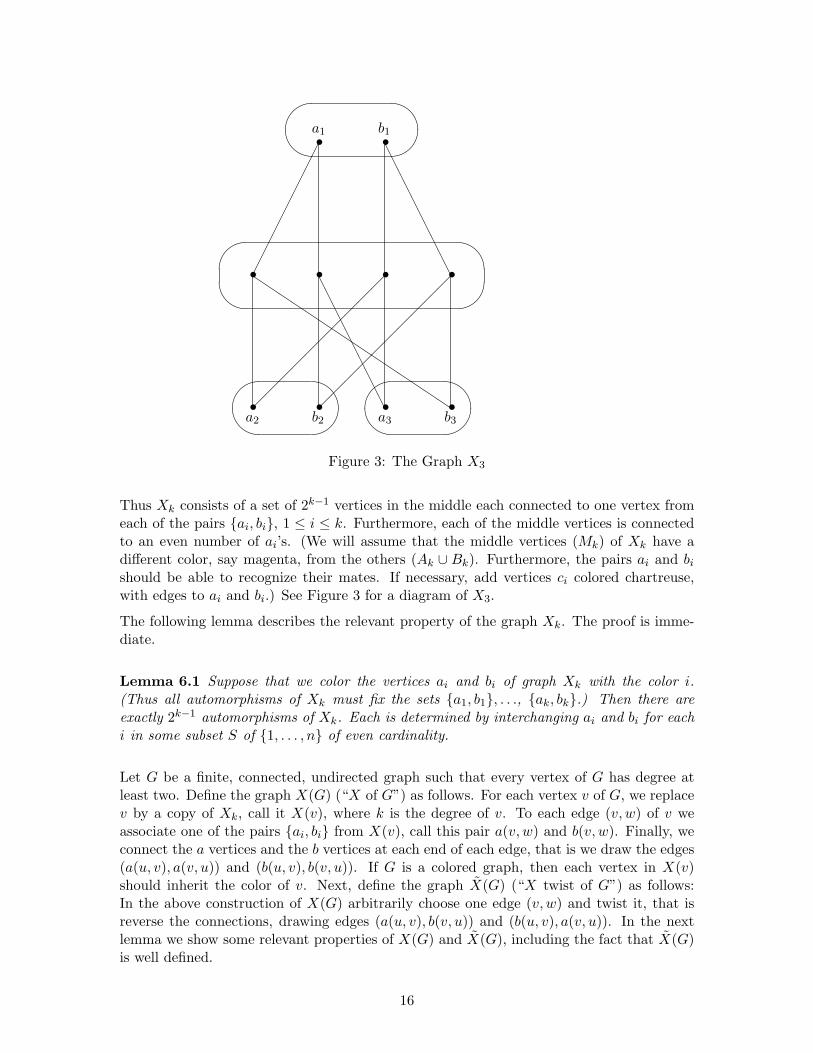
We construct our counterexample graphs by starting with low degree graphs having onlylinear size separators. We replace each vertex v of degree k in such a graph by the graphXk, defined as follows: Xk = (Vk, Ek), where

Vk = Ak ∪Bk ∪Mk where Ak = ai | 1 ≤ i ≤ k,Bk = bi | 1 ≤ i ≤ k, andMk = mS | S ⊆ 1, . . . , k, |S| is even

Ek = (mS , ai) | i ∈ S ∪ (mS , bi) | i 6∈ S

15

'&

$%

'&

$%

'&

$%

'&

$%

•a1

•b1

• • • •

•a2

•b2

•a3

•b3

AA

AA

AA

AA

AA

AA

AA

AA

AA

AA

QQ

QQ

QQ

QQ

QQ

QQ

QQ

Q

Figure 3: The Graph X3

Thus Xk consists of a set of 2k−1 vertices in the middle each connected to one vertex fromeach of the pairs ai, bi, 1 ≤ i ≤ k. Furthermore, each of the middle vertices is connectedto an even number of ai’s. (We will assume that the middle vertices (Mk) of Xk have adifferent color, say magenta, from the others (Ak ∪ Bk). Furthermore, the pairs ai and bishould be able to recognize their mates. If necessary, add vertices ci colored chartreuse,with edges to ai and bi.) See Figure 3 for a diagram of X3.

The following lemma describes the relevant property of the graph Xk. The proof is imme-diate.

Lemma 6.1 Suppose that we color the vertices ai and bi of graph Xk with the color i.(Thus all automorphisms of Xk must fix the sets a1, b1, . . ., ak, bk.) Then there areexactly 2k−1 automorphisms of Xk. Each is determined by interchanging ai and bi for eachi in some subset S of 1, . . . , n of even cardinality.

Let G be a finite, connected, undirected graph such that every vertex of G has degree atleast two. Define the graph X(G) (“X of G”) as follows. For each vertex v of G, we replacev by a copy of Xk, call it X(v), where k is the degree of v. To each edge (v, w) of v weassociate one of the pairs ai, bi from X(v), call this pair a(v, w) and b(v, w). Finally, weconnect the a vertices and the b vertices at each end of each edge, that is we draw the edges(a(u, v), a(v, u)) and (b(u, v), b(v, u)). If G is a colored graph, then each vertex in X(v)should inherit the color of v. Next, define the graph X(G) (“X twist of G”) as follows:In the above construction of X(G) arbitrarily choose one edge (v, w) and twist it, that isreverse the connections, drawing edges (a(u, v), b(v, u)) and (b(u, v), a(v, u)). In the nextlemma we show some relevant properties of X(G) and X(G), including the fact that X(G)is well defined.

16

Lemma 6.2 Let G be any finite, connected graph such that every vertex of G has degree atleast two. Let X(G) and X(G) be as above. Let X(G) be constructed like X(G), but withexactly t of its edges twisted. Then X(G) is isomorphic to X(G) iff t is even, and X(G) isisomorphic to X(G) iff t is odd.

Proof First observe the following fact about X(G). Let v be any vertex of G, and let(x, v), (y, v) be any two edges incident at v. If in X(G) we twist both (x, v) and (y, v), thenthe resulting graph is isomorphic to X(G). (This is immediate from Lemma 6.1.)

Now suppose that the number of twists in t is greater than or equal to two. The aboveobservation lets us move the twists towards each other until they overlap and cancel eachother out. Thus if t is even then X(G) is isomorphic to X(G), otherwise it is isomorphicto X(G).

It remains to show that X(G) is not isomorphic to X(G). Assume for the sake of a contra-diction that ϕ is an isomorphism from X(G) to X(G). Consider the action of ϕ on any paira(v, w), b(v, w) ⊂ X(v), for (v, w) an edge of G. Because of the colorings in the definitionof Xk, ϕ must map the pair a(v, w), b(v, w) to some a(v′, w′), b(v′, w′) in X(G), andthus ϕ also maps a(w, v), b(w, v) to a(w′, v′), b(w′, v′). Define ⊕ϕ to be the sum mod2 over all such pairs in X(G) of the number of times ϕ maps an a to a b. Clearly if weconsider the two pairs corresponding to every edge (x, y) in G, the number of such switchesis either zero or two, except for the unique edge chosen in the construction of X(G), wherethe number is one. Hence ⊕ϕ is one mod 2. Now let’s consider the mod 2 sum in anotherway, namely in terms of each copy of Xk in X(G). By Lemma 6.1, it is immediate that ⊕ϕis zero mod 2. This contradiction proves the lemma.

Definition 6.3 A separator of a graph G = (V,E) is a subset S ⊂ V such that the inducedsubgraph on V − S has no connected component with more than |V |/2 vertices.

We now prove our main theorem:

Theorem 6.4 Let T be a graph such that every separator of T has at least s+ 1 vertices.Then

X(T ) ≡Cs X(T ) .

Proof By Theorem 5.2, it suffices to give a winning strategy for Player II in the Cs gameon X(T ) and X(T ). We will assume that the original graph T has color class size one. Thegraphs X(T ) and X(T ) inherit these colors and so have color class size 2k−1, where k is themaximum degree of any vertex in T . This only makes life more difficult for Player II.

We know by Lemma 6.2 that if we add a twist to any edge of X(T ), then the resulting graphis isomorphic to X(T ). After the rth move of the game, let Qr be the largest connectedcomponent in T −Pr where Pr is the set of vertices g ∈ T such that just after the rth movethere is a pebble on a vertex of X(g) in X(T ). Since T has no s separator, we know thatQr contains over half the vertices of T . Player II’s winning strategy will be to maintain thefollowing property:

17

(∗) For each vertex g ∈ Qr, let Xg(T ) be X(T ) with an edge adjacent to g twisted. Thenthere exists an isomorphism αr,g from Xg(T ) to X(T ), such that for all i ≤ s, αr,g

maps the vertex under pebble xi in X(T ) to the vertex under pebble xi in X(T ).

The difference between X(T ) and X(T ) is that the latter graph has one twisted edge. Anintuitive explanation of Player II’s winning strategy is that she keeps this twisted edgeinside of Qr. With only s pebbles, Player I cannot break apart Qr to expose the twist.

Clearly if Player II can maintain (∗), then the map from the pebbled points in X(T ) tothe corresponding pebbled points in X(T ) is an isomorphism, and she wins. We show byinduction on r, that Player II can maintain (∗). First let us make a remark about PlayerI’s moves. By Observation 5.3, it always suffices for Player I to restrict himself to choosinga set of monochromatic points at each move. Notice that, if Player I chooses a vertex inM(h), the middle of an X(h), then all the other vertices in that X(h) are determined.Furthermore, since one point in M(h) determines all of M(h), it suffices for Player I tochoose only a single point at a time. (Thus counting does not help at all in distinguishingX(T ) from X(T )!)

Player II’s inductive strategy can now be stated. Assume (∗) holds, and suppose that onmove r + 1 Player I picks up pebble xi and puts it down on a vertex in M(w). Note thata new largest component Qr+1 is determined. Let g be a vertex in Qr ∩Qr+1. Player II’sresponse is to answer Player I’s move according to the isomorphism αr,g. To maintain (∗),let αr+1,g = αr,g. Since there is a pebble-free path from g to every other vertex in Qr+1, theproof of Lemma 6.2 shows us how to define all the other isomorphisms, αr+1,h, h ∈ Qr+1.

Corollary 6.5 There exists a sequence of pairs of graphs Gn,Hn, n ∈ N admitting alinear time canonical labeling algorithm and having the following additional properties:

1. Gn and Hn have O(n) vertices.

2. Gn and Hn have degree three and color class size four.

3. Gn ≡Cn Hn.

4. Gn is not isomorphic to Hn.

Proof This follows immediately from Theorem 6.4 when we let Gn = X(Tn) and Hn =X(Tn) where the Tn’s are a sequence of degree three graphs of separator size n, with eachvertex of Tn colored a unique color. Such graphs are well known to exist, see for example[2].

7 Corollaries

A long time ago, one of us showed that there is a polynomial-time property of graphs thatrequires Ω(2

√log n) quantifiers to be expressed in first-order logic without ordering. That

proof also used the graphs X(Dn) and X(Dn), for a certain sequence of degree three graphs

18

Dn [22, Theorem 7]. Now, Corollary 6.5 improves that lower bound to Ω(n) variables.10

It also shows graphically that if we exclude the ordering relation from inductive first-orderlogic, then the addition of counting does not suffice to express all polynomial-time graphproperties. In particular, we have the following:

Corollary 7.1 Let Γ be the set of all graphs of the form X(G), or X(G), for all graphs Gof degree at most three and color class size one. Then the isomorphism problems for graphsin Γ is expressible in first-order logic with ordering and sum mod 2, but it is not expressibleby any sequence of first-order sentences from Cr(n) (without ordering), where r(n) = o(n).

Remark 7.2 In particular, inductive logic with counting, but without ordering does notcontain all the polynomial-time computable graph properties. In fact, it does not even con-tain all such properties computable by a uniform sequence of bounded-depth, polynomial-sizeBoolean circuits that include parity gates, cf. [12].

Proof We have seen in Corollary 6.5 that the graphs X(Tn) and X(Tn) are indistinguish-able in Cεn for some constant ε > 0. Suppose for the sake of a contradiction that there werea sentence σ ∈ (FO + LFP + COUNT) that expresses the isomorphism property for graphsfrom Γ. That is for graphs G,H ∈ Γ,

(G,H) |= σ ⇔ G ∼= H

Let k be the number of distinct variables occurring in σ. For graphs of size n, let σn

be the unwinding of σ as follows. Rewrite any least fixed points of arity a, (LFPϕ) asϕ(na)(∅). Next replace any quantified number variable ∃i (respectively, ∀i) by a disjunctionn−1∨i=0

(respectively, by a conjunctionn−1∧i=0

). Note that σn ∈ Ck and is equivalent to σ for

structures of size at most n.

Thus we have that σn distinguishes the pair P = (X(Tn), X(Tn)) from the pair Q =(X(Tn), X(Tn)). It follows that Player I wins the Ck game on these two pairs. Note thatPlayer II can match any vertex in the first X(Tn) from P with the same vertex in the firstX(Tn) from Q. Thus, Player I must have a winning strategy for the Ck game on X(Tn) andX(Tn). This contradiction shows that isomorphism for graphs from Γ is not expressible in(FO + LFP + COUNT).

We next show that we can distinguish X(G) from X(G) in first-order logic with orderingand sum mod 2. This is easy. The ordering gives us a way to mark each of the pairs a(g, h)and b(g, h) in the graphs. Let a(g, h) be the first of the pair, and b(g, h) the second. (Notethat since the vertices in M(g) and M(h) inherit unique colors from g and h, we are givenas part of the input which pair of vertices is a(g, h), b(g, h).) Now, given this assignmentof a’s and b’s, a simple first-order sentence asserts that X(g) is straight (i.e. isomorphic toX3) or twisted (i.e. each vertex in M(g) is adjacent to an odd number of a’s). Now, thegraph is isomorphic to X(G) iff the sum mod 2 of the number of twisted vertices and edgesis 0, and it’s isomorphic to X(G) iff the sum mod 2 is 1.

10This is a major improvement because n is much bigger than 2√

log n, and because a sentence withq quantifiers can make use of at most q variables, but a sentence with v variables can make use of 2nv

quantifiers.

19

Of course, if G 6= H, then since these graphs have color class size one, X(G) and X(H) canbe distinguished by a sentence in L2. Thus isomorphism for graphs from Γ is expressible inAC0 plus parity gates, as claimed.

The next result proves a straightforward upper bound that nearly matches our lower boundon the number of variables needed to identify a class ∆ of graphs as a function of theseparator size of members of ∆.

Proposition 7.3 Let ∆ be a set of graphs closed under induced subgraphs, such that everygraph G ∈ ∆ has a separator of size at most s(n), where n is the number of vertices of G.Then ∆ is identified by CV (n) where

V (n) = 3 +blog nc∑

i=0

s(bn2−ic) .

(In particular, V (n) ≤ s(n) log n, and if s(n) = nα, then V (n) = O(s(n)).)

Proof We use induction on n, the number of vertices of G. Given G, we can first say thatthere exist vertices x1, . . . , xs(n) such that every connected component of G − xi|1 ≤ i ≤s(n) has size at most bn/2c. This is expressible in s(n) + 3 variables. Next we assert howmany connected components of each isomorphism type there are. This requires V (bn/2c)variables, in addition to the s(n) that we leave on x1, . . . , xs(n).

8 Conclusions and Open Questions

1. We redirect the reader’s attention to Questions 3.2 and 3.3. We have shown in Corol-lary 6.5 that first-order logic plus counting and least fixed point, but without ordering,fails badly. The question,“What besides counting must be added to FO + LFP to getall polynomial-time graph problems?” is worthy of much study, cf. [27, 20].

2. Planar graphs have separators of size O(√n), and thus by Proposition 7.3 they can

be identified in C√n. However, Theorem 6.4 does not give a matching lower boundbecause even if G is planar, the graph X(G) need not be. We would like to know ifΩ(√n) variables are necessary to identify planar graphs.

Acknowledgements: Thanks to Sandeep Bhatt who improved our results by pointingout that the essential property of the counterexample graphs we were using was that theirseparators are large. Thanks to Laci Babai for informing us about the status of the researchon the W-L method in the Soviet Union.

References

[1] A.V. Aho, J.E. Hopcroft and J.D. Ullman, The Design and Analysis of ComputerAlgorithms, Addison-Wesley (1974).

20

[2] M. Ajtai, “Recursive Construction for 3-Regular Expanders,” 28th IEEE Symp. onFoundations of Computer Science (1987), 295-304.

[3] Laszlo Babai, “Monte Carlo Algorithms in Graph Isomorphism Testing,” Tech. Rep.DMS 79-10, Universite de Montreal, 1979.

[4] Laszlo Babai, “On the Complexity of Canonical Labeling of Strongly Regular Graphs,”SIAM J. Computing 9 (1980), 212-216.

[5] Laszlo Babai, “Moderately Exponential Bound for Graph Isomorphism,” Proc. Conf.on Fundamentals of Computation Theory, Lecture Notes in Computer Science,Springer, 1981, 34-50.

[6] Laszlo Babai, “On the Order of Uniprimitive Permutation Groups,” Annals of Math.113 (1981), 553-568.

[7] Laszlo Babai, “Permutation Groups, Coherent Configurations, and Graph Isomor-phism,” D.Sc. Thesis, Hungarian Acad. Sci., 1984 (in Hungarian).

[8] Laszlo Babai, Paul Erdos, and Stanley M. Selkow, “Random Graph Isomorphism,”SIAM J. on Comput. 9 (1980), 628-635.

[9] L. Babai, W.M. Kantor, and E.M. Luks, “Computational Complexity and the Clas-sification of Finite Simple Groups,” 24th IEEE Symp. on Foundations of ComputerScience (1983), 162-171.

[10] Laszlo Babai and Ludek Kucera, “Canonical Labelling of Graphs in Linear AverageTime,” 20th IEEE Symp. on Foundations of Computer Science (1979), 39-46.

[11] Laszlo Babai and Eugene M. Luks, “Canonical Labeling of Graphs,” 15th ACM Sym-posium on Theory of Computing (1983), 171-183.

[12] David Mix Barrington, Neil Immerman, and Howard Straubing, “On UniformityWithin NC1,” J. Comput. System Sci. 41, No. 3 (1990), 274-306.

[13] Laszlo Babai and Rudi Mathon, Talk at the South-East Conference on Combinatoricsand Graph Theory, 1980.

[14] P.J. Cameron, “6-Transitive Graphs,” J. Combinat. Theory B 28, (1980), 168-179.[15] Ashok Chandra and David Harel, “Structure and Complexity of Relational Queries,”

J. Comput. System Sci. 25 (1982), 99-128.[16] A. Ehrenfeucht, “An Application of Games to the Completeness Problem for Formal-

ized Theories,” Fund. Math. 49 (1961), 129-141.[17] R. Fraısse, “Sur quelques classifications des systems de relations,” Publ. Sci. Univ.

Alger 1 (1954), 35-182.[18] Martin Furer, Walter Schnyder, and Ernst Specker, “Normal Forms for Trivalent

Graphs and Graphs of Bounded Valence,” 15th ACM Symposium on Theory of Com-puting (1983), 161-170.

[19] Ya. Yu. Gol’fand and M.H. Klin, “On k-Regular Graphs,” in Algorithmic Research inCombinatorics, Nauka Publ., Moscow, 1978, 76-85.

[20] Yuri Gurevich, “Logic and the Challenge of Computer Science,” in Current Trends inTheoretical Computer Science, ed. Egon Borger, Computer Science Press, 1988, 1-57.

[21] D.G. Higman, “Coherent Configurations I.: Ordinary Representation Theory,” Geome-triae Dedicata 4 (1975), 1-32.

[22] Neil Immerman, “Number of Quantifiers is Better than Number of Tape Cells,” J.Comput. System Sci. 22, No. 3 (1981), 384-406.

[23] Neil Immerman, “Upper and Lower Bounds for First Order Expressibility,” J. Comput.System Sci. 25, No. 1 (1982), 76-98.

21

[24] Neil Immerman, “Relational Queries Computable in Polynomial Time,” Informationand Control 68 (1986), 86-104.

[25] Neil Immerman, “Languages That Capture Complexity Classes,” SIAM J. Computing16, No. 4 (1987), 760-778.

[26] Neil Immerman and Dexter Kozen, “Definability with Bounded Number of BoundVariables,” Information and Computation 83 (1989), 121-139.

[27] Neil Immerman and Eric S. Lander, “Describing Graphs: A First-Order Approach toGraph Canonization,” in Complexity Theory Retrospective, Alan Selman, ed., Springer-Verlag, 1990, 59-81.

[28] N. Immerman, S. Patnaik, and D. Stemple, “The Expressiveness of a Family of FiniteSet Languages,” Tenth ACM Symposium on Principles of Database Systems (1991),37-52.

[29] Ludek Kucera, “Canonical Labeling of Regular Graphs in Linear Average Time,” 28thIEEE Symp. on Foundations of Computer Science (1987), 271-279.

[30] M.H. Klin, M.E. Muzichuk, and I.A. Faradzev, “Cellular Rings and Groups of Auto-morphisms of Graphs,” Introductory Article to a Book to be Published by D. ReidelPubl. Co.

[31] M.Ch. Klin, R. Poschel, and K. Rosenbaum, “Angewandte Algebra,” Vieweg & SohnPubl., Braunschweig 1988.

[32] R. Lipton, “The Beacon Set Approach to Graph Isomorphism,” Yale Dept. Comp. Sci.preprint No. 135, 1978.

[33] Eugene M. Luks, “Isomorphism of Graphs of Bounded Valence Can be Tested in Poly-nomial Time,” J. Comput. System Sci. 25 (1982), 42-65.

[34] R. Mathon, “A Note On the Graph Isomorphism Counting Problem,” Inform. Proc.Let. 8 (1979), 131-132.

[35] B.D. McKay, “Nauty User’s Guide (Version 1.2),” Tech. Rep. TR-CS-87-03, Dept.Computer Science, Austral. National Univ., Melbourne, 1987.

[36] G.L. Miller, “On the nlog n Isomorphism Technique,” 10th ACM Symposium on Theoryof Computing (1978), 51-58.

[37] R.C. Read and D.G. Corneil, “The Graph Isomorphism Disease,” J. Graph Theory 1(1977), 339-363.

[38] M. Vardi, “Complexity of Relational Query Languages,” 14th ACM Symposium onTheory of Computing (1982), 137-146.

[39] Boris Weisfeiler, ed., On Construction and Identification of Graphs, Lecture Notes inMathematics 558, Springer, 1976.

[40] B. Weisfeiler and A.A. Lehman, “A Reduction of a Graph to a Canonical Form andan Algebra Arising during this Reduction,” (in Russian), Nauchno-TechnicheskayaInformatsia, Seriya 2, 9 (1968), 12-16.

[41] V.N. Zemlyachenko, N. Kornienko, and R.I. Tyshkevich, “Graph Isomorphism Prob-lem,” (in Russian), The Theory fo Computation I, Notes Sci. Sem. LOMI 118, 1982.

22