Embed Size (px)
Citation preview

An Operator Splitting Approach for the InteractionBetween a Fluid and a Multilayered PoroelasticStructureMartina Bukac,1 Ivan Yotov,1 Paolo Zunino2
1Department of Mathematics, University of Pittsburgh, Pittsburgh, Pennsylvania 152602Department of Mechanical Engineering & Materials Science, University of Pittsburgh,Pittsburgh, Pennsylvania 15261
Received 14 February 2014; accepted 18 September 2014Published online 28 November 2014 in Wiley Online Library (wileyonlinelibrary.com).DOI 10.1002/num.21936
We develop a loosely coupled fluid-structure interaction finite element solver based on the Lie operatorsplitting scheme. The scheme is applied to the interaction between an incompressible, viscous, Newtonianfluid, and a multilayered structure, which consists of a thin elastic layer and a thick poroelastic material.The thin layer is modeled using the linearly elastic Koiter membrane model, while the thick poroelasticlayer is modeled as a Biot system. We prove a conditional stability of the scheme and derive error estimates.Theoretical results are supported with numerical examples. © 2014 Wiley Periodicals, Inc. Numer MethodsPartial Differential Eq 31: 1054–1100, 2015
Keywords: fluid-structure interaction; loosely coupled scheme; poroelasticity
I. INTRODUCTION
Many natural materials—including soil, wood, and some biological tissues—have a multilayeredstructure consisting of two or more constituent materials. Multilayered structures can have dis-tinct properties from their constituent materials. This characteristic is often used in engineering toproduce a new material which is stiffer or lighter when compared to traditional materials. In manycases, such structures are surrounded by a fluid. In this setting, we are interested in permeablestructures. Examples of multilayered permeable structure that are in contact with a fluid can befound in groundwater flow modeling, reservoir engineering, and modeling of blood flow through
Correspondence to: M. Bukac, Department of Applied and Computational Mathematics and Statistics, University of NotreDame, Notre Dame, IN 46556 (e-mail: [email protected])Contract grant sponsor: NSF (to M.B.); contract grant number: DMS 1216465Contract grant sponsor: Mathematics Research Center, University of Pittsburgh (to M.B.)Contract grant sponsor: NSF (to I.Y.); contract grant number: DMS 1115856Contract grant sponsor: DOE (to I.Y.); contract grant number: DE-FG02-04ER25618Contract grant sponsor: DOE (to P.Z.); contract grant number: DE-FG02-04ER25618Contract grant sponsor: NSF (to P.Z.); contract grant number: DMS 1311983
© 2014 Wiley Periodicals, Inc.

FLUID-POROELASTIC STRUCTURE INTERACTION 1055
the major blood vessels. Thus, in order to detect the damage in a reservoir or certain pathologiesof blood vessels, it is important to understand the interaction between a fluid and a multilayeredpermeable structure.
We study the interaction between an incompressible viscous, Newtonian fluid and a multi-layered poroelastic structure. This model features two different kinds of coupling, each widelystudied in the literature: the flow-porous media coupling [1–10] and the fluid-structure coupling[11–20]. Main challenges in the flow-porous media interaction problems arise from the couplingof two domains, a fluid region and a porous media region, along with the two physical processesoccurring in each region. Introducing the poroelastic media, our domain becomes time dependent,and thus we must resolve difficulties related to a moving domain. Furthermore, classical parti-tioned solvers for the fluid-structure interaction (FSI) problems are known to have stability issueswhen the density of the structure is comparable to the density of the fluid [21]. This difficulty willbe taken into account here, since in this work we are interested on applications in hemodynamics,among others, and the density of blood is almost equal to the density of blood vessels.
The material properties of arteries have been widely studied [22–28]. Pseudoelastic [25, 29],viscoelastic [22–24], and nonlinear material models represent well known examples. To ourknowledge, only a few of them have been deeply analyzed in the time dependent domain, namelywhen coupled with the pulsation induced by heartbeat. These considerations also apply to poro-elasticity, which is addressed here. Poroelasticity becomes particularly interesting when lookingat the coupling of flow with mass transport. This is a significant potential application of ourmodel, as mass transport provides nourishment, removes wastes, affects pathologies, and allowsto deliver drugs to arteries [30]. Poroelastic phenomena are interesting in different applicationswhere soft biological tissues are involved. We mention for example cerebro-spinal flow [31],which also involves FSI, the study of hysteresis effects observed in the myocardial tissue [32, 33],as well as the modeling of lungs as a continuum material [34]. Besides biological applications,this model can also be used in numerous other applications: geomechanics, ground-surface waterflow, reservoir compaction and surface subsidence, seabed-wave interaction problem, and soforth.
Although there exist many complex and detailed models for mutilayered structures in differentapplications, the interaction between the fluid and a multilayered structure remains an area ofactive research. To our knowledge, the only theoretical result was presented in [18], where theauthors proved existence of a solution to a fluid-two-layered-structure interaction problem, inwhich one layer is modeled as a thin (visco)elastic shell and the other layer as a linearly elasticstructure. Several studies focused on numerical simulations. An interaction between the fluidand a two-layer anisotropic elastic structure was used in [35] to model the human right and leftventricles. Slightly different models were used in [36] to model fully coupled fluid-structure-soilinteraction for cylindrical liquid-contained structures subjected to horizontal ground excitation.The work in [37] focused on studying velocity of acoustic waves excited in multilayered structuresin contact with fluids. A fluid-multilayered structure interaction problem coupled with transportwas studied in [38], with the purpose of investigating low-density lipoprotein transport within amultilayered arterial wall. However, none of these studies present a numerical scheme supportedwith stability and error analysis.
In this work, we propose a model that captures interaction between a fluid and a multilayeredstructure, which consists of a thin elastic layer and a thick poroelastic layer. In the context ofcardiovascular applications, we assume that the thin layer represents a homogenized combinationof the endothelium, tunica intima, and internal elastic lamina, and that the thick layer representstunica media. The thin elastic layer is modeled using the linearly elastic Koiter membrane model,while the poroelastic medium is modeled using the Biot equations. The Biot system consists of
Numerical Methods for Partial Differential Equations DOI 10.1002/num
1056 BUKAC, YOTOV, AND ZUNINO
an elastic skeleton and connecting pores filled with fluid. We assume that the elastic skeleton ishomogeneous and isotropic, while the fluid in the pores is modeled using the Darcy equations.The Biot system is coupled to the fluid and the elastic membrane via the kinematic (no-slip andconservation of mass) and dynamic (conservation of momentum) interface conditions. More pre-cisely, we assume that the elastic membrane cannot store fluid, but allows the flow through it in thenormal direction. In the tangential direction, we prescribe the no-slip boundary condition. Thisassumption is reasonable in blood flow modeling, as it has been shown in [39] that predominantdirection of intimal transport is the radial direction normal to the endothelial surface, for all rangesof relative intimal thickness.
The coupling between a fluid and a single layer poroelastic structure has been previouslystudied in [12, 40–44]. In [40], the authors analyze the problem form the physical standpoint,with the aim to identify the differences between a poroelastic model and a purely elastic one onthe propagation of pressure waves and the deformation of the arterial walls using a simplifiedFSI benchmark for blood flow in arteries. Since those numerical tests are not computationallyexpensive, the numerical solver is based on a monolithic approach, where the interface conditionsare enforced using Nitsche’s method. Other authors have already analyzed the problem from thenumerical perspective. In particular, the work in [45] is based on the modeling and a numeri-cal solution of the interaction between an incompressible, Newtonian fluid, described using theNavier–Stokes equations, and a poroelastic structure modeled as a Biot system. The problemwas solved using both a monolithic and a partitioned approach. The partitioned approach wasbased on the domain decomposition procedure, with the purpose of solving the Navier–Stokesequations separately from the Biot system. However, subiterations were needed between the twoproblems due to the instabilities associated with the “added mass effect.” Namely, in FSI prob-lems, the “classical” loosely coupled methods have been shown to be unconditionally unstable ifthe density of the structure is comparable to the density of the fluid [21, 46], which is the casein hemodynamics applications. To resolve this problem, several different splitting strategies havebeen proposed [11, 13, 15, 19, 20, 47–57]. More precisely, in [11], the authors present a stronglycoupled partitioned scheme based on Robin-type coupling conditions. In addition to the classicalDirichlet–Neumann and Neumann–Dirichlet schemes, they also propose a Robin–Neumann anda Robin–Robin scheme, that converge without relaxation, and need a smaller number of subitera-tion between the fluid and the structure in each time step than classical strongly coupled schemes,provided that the interface parameters are suitably chosen, see [45, 58].
In [50, 59], Burman and Fernández propose an explicit scheme where the coupling betweenthe fluid and a thick structure is enforced in a weak sense using Nitsche’s approach [16]. Theformulation in [50] still suffers from stability issues, which were corrected by adding a weaklyconsistent stabilization term that includes pressure variations at the interface. The splitting error,however, lowers the temporal accuracy of the scheme, which was then corrected by proposing afew defect-correction subiterations to achieve an optimal convergence rate.
A novel loosely coupled partitioned scheme, called the kinematically coupled scheme, wasintroduced by Guidoboni et al. in [56], and applied to FSI problems with thin structures. Thescheme is based on embedding the no-slip kinematic condition into the thin structure equations.Using the Lie operator splitting approach [60], the structure equations are split so that the struc-ture inertia is treated together with the fluid as a Robin boundary condition, while the structureelastodynamics is treated separately. This method has been shown to be unconditionally stable,and therefore, independent of the fluid and structure densities. Stability is achieved by combiningthe structure inertia with the fluid subproblem to mimic the energy balance of the continuousproblem. Additionally, Muha and Canic showed that the scheme converges to a weak solution ofthe fully nonlinear FSI problem [61].
Numerical Methods for Partial Differential Equations DOI 10.1002/num

FLUID-POROELASTIC STRUCTURE INTERACTION 1057
The main features of the kinematically coupled scheme are simple implementation, modu-larity, no need for subiterations between the fluid and structure subproblems, and very goodperformance in terms of stability, accuracy, and computational cost. Hence, modifications of thisscheme have been used by several authors to study different multiphysics problems involvingFSI. A modification of the scheme was proposed by Lukácová-Medvid’ová et al. to study FSIinvolving non-Newtonian fluids [17, 62]. An extension of the kinematically coupled scheme wasproposed in [13] where a parameter β was introduced to increase the accuracy. It was shown in[13] that the accuracy of the kinematically coupled β-scheme with β = 1 is comparable to that ofmonolithic scheme by Badia et al., in [49] when applied to a nonlinear benchmark FSI problem inhemodynamics. A modified kinematically coupled scheme, called “the incremental displacement-correction scheme,” that treats the structure displacement explicitly in the fluid substep and thencorrects it in the structure substep was recently proposed by Fernández et al. [15, 53, 55].
Inspired by the kinematically coupled scheme, in this manuscript we propose a loosely cou-pled finite element scheme for the fluid-membrane-poroelastic structure interaction problembased on the Lie operator splitting method. We use the operator splitting to separate the fluidproblem (Navier–Stokes equations) from the Biot problem. The no-slip kinematic condition inthe tangential direction is embedded into the membrane equations. We recall that this coupledproblem is particularly challenging, because it combines the free fluid-porous media flow andthe fluid-structure coupling mechanisms. This work shows that the kinematically coupled Liesplitting method can be successfully applied also in this case. In particular, the operator split-ting is performed so that the tangential component of the structure inertia is treated togetherwith the fluid as a Robin boundary condition. Assuming the pressure formulation for the Darcyequations, the continuity of the normal flux and the balance of normal components of stressbetween the Navier–Stokes fluid and the fluid in the pores is treated in a similar way as inthe partitioned algorithms for the Stokes–Darcy coupled problems [6, 63]. The membrane elas-todynamics is embedded into the Biot system as a Robin boundary condition. In contrast withdomain decomposition methods proposed in [12], the operator splitting approach does not requiresubiterations between the fluid and the Biot problem, making our scheme more computationallyefficient.
We prove a conditional stability of the proposed scheme, where the stability condition does notdepend on the fluid and structure densities, but it is related to the decoupling of the Stokes–Darcyinteraction problem. Furthermore, we derive error estimates and prove the convergence of thescheme. The rates of convergence and the stability condition are validated numerically on aclassical benchmark problem typically used to test the results of FSI algorithms. In a secondnumerical example, we investigate the effects of porosity on the structure displacement. Namely,we consider a high storativity and a high permeability case in the Darcy equations, and comparethem to the results obtained using a purely elastic model. Depending on the regime, we observea significantly different behavior of the coupled system. This conclusion is also supported by thesensitivity analysis, based on both theoretical and numerical approach, addressed by the authorsin [40].
At the level of numerical approximation, we adopt rather standard techniques, based on loworder finite differences and Lagrangian finite elements for the discretization of the equations intime and space, respectively. Indeed, the main contributions of this work arise in the design of thesplitting scheme. In particular, we propose a novel model to study interaction between a fluid anda composite poroelastic structure, and a novel, loosely coupled numerical scheme. The scheme isbased on existing works [5, 56], which were combined and modified to resolve both issues duethe fluid-structure coupling, and the fluid-porous medium coupling. We present the stability andconvergence analysis of the proposed scheme, completed with the numerical examples.
Numerical Methods for Partial Differential Equations DOI 10.1002/num

1058 BUKAC, YOTOV, AND ZUNINO
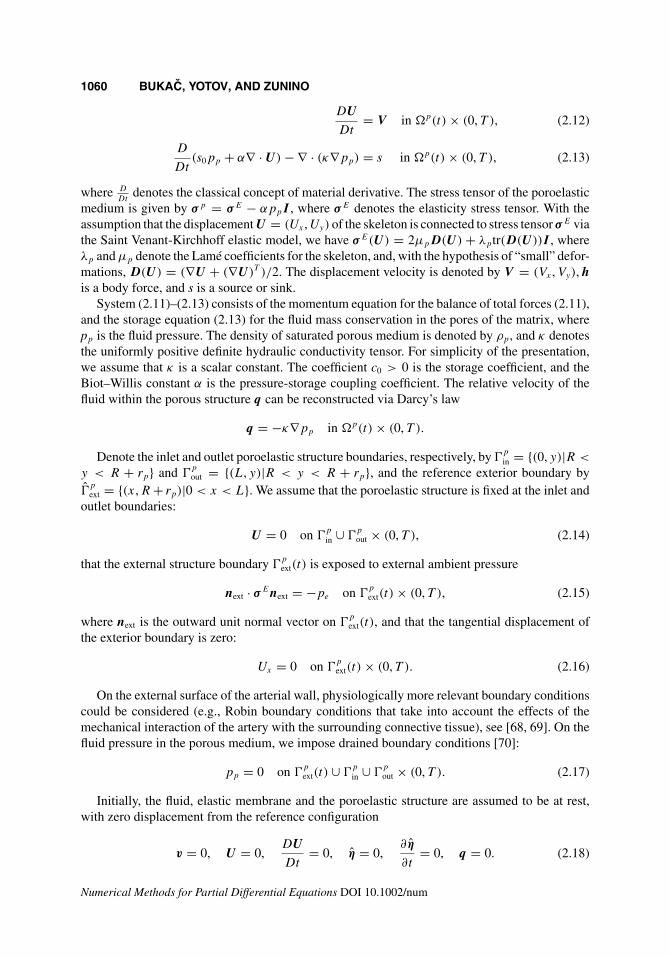
FIG. 1. Deformed domains �f (t) ∪ �p(t).
The rest of the article is organized as follows. In the following section, we introduce the modelequations and the coupling conditions. In Section III, we propose a loosely coupled scheme basedon the operator-splitting approach. The weak formulation and stability of the scheme is presentedin Section IV. In Section V, we derive the error analysis of the scheme. Finally, the numericalresults are presented in Section VI.
II. DESCRIPTION OF THE PROBLEM
Consider a bounded, deformable, two-dimensional domain �(t) = �f (t) ∪ �p(t) of referencelength L, which consists of two regions, �f (t) and �p(t), see Fig. 1. We assume that the region�f (t) has reference width 2R, and is filled by an incompressible, viscous fluid. We denote thewidth of the second region �p(t) by rp, and assume that �p(t) is occupied by a fully saturatedporoelastic matrix. The two regions are separated by a common interface �(t). We assume that�(t) has a mass, and represents a thin, elastic structure. Namely, we assume that the thicknessof the interface rm is “small” with respect to the radius of the fluid domain, rm � R. Thus, thevolume of the interface is negligible, so it acts as a membrane that cannot store fluid, but allowsthe flow through it in the normal direction.
We are interested in simulating a pressure-driven flow through the deformable channel with atwo-way coupling between the fluid, thin elastic interface, and poroleastic structure. Without lossof generality, we restrict the model to a two-dimensional (2D) geometrical model representinga deformable channel. We consider only the upper half of the fluid domain supplemented by asymmetry condition at the axis of symmetry. Thus, the reference fluid and structure domains inour problem (showed by dashed lines in Fig. 1) are given, respectively, by
�f := {(x, y)|0 < x < L, 0 < y < R},�p := {(x, y)|0 < x < L, R < y < R + rp},
and the reference lateral boundary by � = {(x, R)|0 < x < L}. The inlet and outlet fluidboundaries are defined, respectively, as �
f
in = {(0, y)|0 < y < R} and �fout = {(L, y)|0 < y < R}.
We model the flow using the Navier–Stokes equations for a viscous, incompressible, Newtonianfluid:
ρf
(∂v
∂t+ v · ∇v
)= ∇ · σf + g in �f (t) × (0, T ), (2.1)
∇ · v = 0 in �f (t) × (0, T ), (2.2)
Numerical Methods for Partial Differential Equations DOI 10.1002/num

FLUID-POROELASTIC STRUCTURE INTERACTION 1059
where v = (vx , vy) is the fluid velocity, σf = −pf I + 2μf D(v) is the fluid stress tensor, g
is a body force, pf is the fluid pressure, ρf is the fluid density, μf is the fluid viscosity, andD(v) = (∇v + (∇v)T )/2 is the rate-of-strain tensor. Denote the inlet and outlet fluid boundariesby �
f
in and �fout, respectively. At the inlet and outlet boundary, we prescribe the normal stress:
σf nin = −pin(t)nin on �f
in × (0, T ), (2.3)
σf nout = 0 on �fout × (0, T ), (2.4)
where nin/nout are the outward normals to the inlet/outlet fluid boundaries, respectively. Theseboundary conditions are common in blood flow modeling [45, 64, 65] even though they are notphysiologically optimal as the flow distribution and pressure field in the modeled domain areoften unknown [66]. More physiological boundary conditions could be considered, for example,boundary conditions including effects of peripheral resistance, see [66, 67]. Along the middle lineof the channel �
f
0 = {(x, 0)|0 < x < L}, we impose the symmetry conditions:
∂vx
∂y= 0, vy = 0 on �
f
0 × (0, T ). (2.5)
The lateral boundary represents a deformable, thin elastic wall, whose dynamics is modeledby the linearly elastic Koiter membrane model, given in the first-order Lagrangian formulationby:
ρmrm
∂ξx
∂t− C2
∂ηy
∂x− C1
∂2ηx
∂x2= fx on � × (0, T ), (2.6)
ρmrm
∂ξy
∂t+ C0ηy + C2
∂ηx
∂x= fy on � × (0, T ), (2.7)
∂ η
∂t= ξ on � × (0, T ), (2.8)
where η(x, t) = (ηx(x, t), ηy(x, t)) denotes the axial and radial displacement, ξ(x, t) =(ξx(x, t), ξy(x, t)) denotes the axial and radial structure velocity, f = (fx , fy) is a vector ofsurface density of the force applied to the membrane, ρm denotes the membrane density and
C0 = rm
R2
(2μmλm
λm + 2μm
+ 2μm
), C1 = rm
(2μmλm
λm + 2μm
+ 2μm
), C2 = rm
R
2μmλm
λm + 2μm
.
(2.9)
The coefficients μm and λm are the Lamé coefficients for the membrane. Note that we can writethe system (2.6)–(2.7) more compactly as
ρmrm
∂ ξ
∂t+ Lη = f , L :=
(−C1∂xx −C2∂x
C2∂x C0
). (2.10)
The fluid domain is bounded by a deformable porous matrix consisting of a skeleton andconnecting pores filled with fluid, whose dynamics is described by the Biot model, which in thefirst-order, primal, Eulerian formulation reads as follows:
ρp
DV
Dt− ∇ · σ p = h in �p(t) × (0, T ), (2.11)
Numerical Methods for Partial Differential Equations DOI 10.1002/num
1060 BUKAC, YOTOV, AND ZUNINO
DU
Dt= V in �p(t) × (0, T ), (2.12)
D
Dt(s0pp + α∇ · U) − ∇ · (κ∇pp) = s in �p(t) × (0, T ), (2.13)
where D
Dtdenotes the classical concept of material derivative. The stress tensor of the poroelastic
medium is given by σ p = σE − αppI , where σE denotes the elasticity stress tensor. With theassumption that the displacement U = (Ux , Uy) of the skeleton is connected to stress tensor σE viathe Saint Venant-Kirchhoff elastic model, we have σE(U) = 2μpD(U) + λptr(D(U))I , whereλp and μp denote the Lamé coefficients for the skeleton, and, with the hypothesis of “small” defor-mations, D(U) = (∇U + (∇U)T )/2. The displacement velocity is denoted by V = (Vx , Vy), his a body force, and s is a source or sink.
System (2.11)–(2.13) consists of the momentum equation for the balance of total forces (2.11),and the storage equation (2.13) for the fluid mass conservation in the pores of the matrix, wherepp is the fluid pressure. The density of saturated porous medium is denoted by ρp, and κ denotesthe uniformly positive definite hydraulic conductivity tensor. For simplicity of the presentation,we assume that κ is a scalar constant. The coefficient c0 > 0 is the storage coefficient, and theBiot–Willis constant α is the pressure-storage coupling coefficient. The relative velocity of thefluid within the porous structure q can be reconstructed via Darcy’s law
q = −κ∇pp in �p(t) × (0, T ).
Denote the inlet and outlet poroelastic structure boundaries, respectively, by �p
in = {(0, y)|R <
y < R + rp} and �pout = {(L, y)|R < y < R + rp}, and the reference exterior boundary by
�pext = {(x, R + rp)|0 < x < L}. We assume that the poroelastic structure is fixed at the inlet and
outlet boundaries:
U = 0 on �p
in ∪ �pout × (0, T ), (2.14)
that the external structure boundary �pext(t) is exposed to external ambient pressure
next · σEnext = −pe on �pext(t) × (0, T ), (2.15)
where next is the outward unit normal vector on �pext(t), and that the tangential displacement of
the exterior boundary is zero:
Ux = 0 on �pext(t) × (0, T ). (2.16)
On the external surface of the arterial wall, physiologically more relevant boundary conditionscould be considered (e.g., Robin boundary conditions that take into account the effects of themechanical interaction of the artery with the surrounding connective tissue), see [68, 69]. On thefluid pressure in the porous medium, we impose drained boundary conditions [70]:
pp = 0 on �pext(t) ∪ �
p
in ∪ �pout × (0, T ). (2.17)
Initially, the fluid, elastic membrane and the poroelastic structure are assumed to be at rest,with zero displacement from the reference configuration
v = 0, U = 0,DU
Dt= 0, η = 0,
∂ η
∂t= 0, q = 0. (2.18)
Numerical Methods for Partial Differential Equations DOI 10.1002/num

FLUID-POROELASTIC STRUCTURE INTERACTION 1061
A. The Coupling Conditions
To prescribe the coupling conditions on the physical fluid-structure interface �(t), let η be themembrane displacement in the physical configuration and ξ = Dη
Dt. While the lumen and the
poroelastic medium contain fluid, we assume that the elastic membrane does not contain fluid,but allows the flow through it in the normal direction. This is a reasonable assumption becausethe elastic membrane represents tunica intima. It has been shown by experimental studies that thenormal transport in tunica intima is significantly greater than tangential transport [39]. Denoteby n the outward normal to the fluid domain and by τ the tangential unit vector. Thus, the fluid,elastic membrane and poroelastic structure are coupled via the following boundary conditions:
• Mass conservation: since the thin lamina allows the flow through it, the continuity of normalflux is
v · n =(
DU
Dt− κ∇pp
)· n on �(t). (2.19)
• As the permeability of the blood vessels is rather small and we do not allow filtration in thetangential direction, we prescribe no-slip boundary conditions between the fluid in the lumenand the elastic membrane, and between the elastic membrane and poroelastic medium:
v · τ = ξ · τ , η = U on �(t). (2.20)
• Balance of normal components of the stress in the fluid phase:
n · σ f n = −pp on �(t). (2.21)
• The conservation of momentum describes balance of contact forces. Precisely, it says thatthe sum of contact forces at the fluid-porous medium interface is equal to zero:
σ f n − σpn + J −1f = 0 on �(t), (2.22)
where f := f ◦ (A−1t |�(t)), and J denotes the Jacobian of the transformation from �(t) to � given
by
J =√(
1 + ∂ηx
∂x
)2
+(
∂ηy
∂x
)2
. (2.23)
B. The Problem Formulation in the Arbitrary Lagrangian–Eulerian Framework
To deal with the motion of the fluid domain, we adopt the Arbitrary Lagrangian–Eulerian (ALE)approach [65, 71, 72]. In the context of finite element method approximation of moving-boundaryproblems, ALE method deals efficiently with the deformation of the mesh, especially at the bound-ary and near the interface between the fluid and the structure, and with the issues related to theapproximation of the time-derivatives ∂v/∂t ≈ (v(tn+1) − v(tn))/ t which, due to the fact that�f (t) depends on time, is not well defined as the values v(tn+1) and v(tn) correspond to the valuesof v defined at two different domains. Following the ALE approach, we introduce two familiesof (arbitrary, invertible, smooth) mappings At and St , defined on reference domains �f and �p,respectively, which track the domain in time:
At : �f → �f (t) ⊂ R2, x = At (x) ∈ �f (t), for x ∈ �f , (2.24)
St : �p → �p(t) ⊂ R2, x = St (x) ∈ �p(t), for x ∈ �p. (2.25)
Numerical Methods for Partial Differential Equations DOI 10.1002/num
1062 BUKAC, YOTOV, AND ZUNINO
Note that the fluid domain is determined by the displacement of the membrane η, while theporous medium domain is determined by its displacement U , where U is the displacement of theporous medium evaluated at the reference configuration. However, we can define a homeomor-phism over �f (t) ∪ �p(t) by setting mappings At and St equal on �(t). For the structure, weadopt the material mapping
St (x) = x + U(x, t), ∀x ∈ �p. (2.26)
Since the mapping At is arbitrary, with the only requirement that it matches St on �(t), wecan define At as
At (x) = x + Ext(η(x, t)) = x + Ext(U(x, t)|�), ∀x ∈ �f . (2.27)
We do not have to transfer the time-derivatives in the Biot system and in Koiter membraneequations to the reference domain as the material time-derivative is suitable for the time dis-cretization, and the membrane equations are given on the reference configuration. Our problem inthe ALE formulation reads as follows: given t ∈ (0, T ), find v = (vx , vy), pf , η = (ηx , ηy), ξ =(ξx , ξy), U = (Ux , Uy), V = (Vx , Vy) and pp, with η(x, t) = η(A−1
t (x), t), for x ∈ �(t), such that
ρf
(∂v
∂t
∣∣∣∣x
+ (v − w) · ∇v
)= ∇ · σf + g in �f (t) × (0, T ), (2.28a)
∇ · v = 0 in �f (t) × (0, T ), (2.28b)
ρmrm
∂ ξ
∂t+ Lη = f on � × (0, T ), (2.28c)
ρmrm
(ξ − ∂ η
∂t
)= 0 on � × (0, T ), (2.28d)
ρp
DV
Dt= ∇ · σ p + h in �p(t) × (0, T ), (2.28e)
s0D
Dtpp + α∇ · DU
Dt− ∇ · (κ∇pp) = s in �p(t) × (0, T ), (2.28f)
ρp
(V − DU
Dt
)= 0 in �p(t) × (0, T ), (2.28g)
with the kinematic coupling conditions on �(t):
ξ · τ = v · τ , η = U , (2.29)
dynamic coupling conditions on �(t):
σ f n − σpn + J −1f = 0, (2.30)
n · σ f n = −pp, (2.31)
and the continuity of normal flux on �(t):
v · n =(
DU
Dt− κ∇pp
)· n, (2.32)
Numerical Methods for Partial Differential Equations DOI 10.1002/num

FLUID-POROELASTIC STRUCTURE INTERACTION 1063
with the boundary and initial conditions given in Section I, where w in (2.28a) denotes the domainvelocity given by
w(x, t) = ∂At (x)
∂t, (2.33)
Denote by L the inverse Piola transformation of L, namely L = J −1LF −T , where F = ∇xAt .Then, composing the Koiter membrane equations (2.10) with A−1
t , using the first condition in(2.29) and condition (2.31), we can write the tangential and normal component of condition (2.30)as follows:
ρmrm
∂v
∂t· τ + τ · Lη + Jτ · σ f n − Jτ · σpn = 0, on �(t) (2.34a)
ρmrm
Dξ
Dt· n + n · Lη − Jpp − Jn · σpn = 0, on �(t). (2.34b)
We will use condition (2.30) written the form (2.34a)–(2.34b) when performing the operatorsplitting.
III. WEAK FORMULATION OF THE MONOLITHIC PROBLEM
For a domain �, we denote by || · ||Hk(�) the norm in the Sobolev space Hk(�). The norm inL2(�) is denoted by ||·||L2(�), and the L2(�)− inner product by (·, ·)�. We introduce the followingbilinear forms
af (v, ϕf ) = 2μf
∫�f (t)
D(v) : D(ϕf )dx,
bf (pf , ϕf ) =∫
�f (t)
pf ∇ · ϕf dx,
ae(U , ϕp) = 2μp
∫�p(t)
D(U) : D(ϕp)dx + λp
∫�p(t)
(∇ · U)(∇ · ϕp)dx,
ap(pp, ψp) =∫
�p(t)
κ∇pp · ∇ψpdx,
bep(pp, ϕp) = α
∫�p(t)
pp∇ · ϕpdx,
am(η, ζ )=rm
∫ L
04μm
((∂ηx
∂x
∂ζx
∂x+ 1
R2ηy ζy
)+ λm
λm + 2μm
(∂ηx
∂x+ 1
Rηy
) (∂ζx
∂x+ 1
Rζy
))dx
cfp(pp, ϕf ) =∫
�(t)
ppϕf · ndx,
cep(pp, ϕp) =∫
�(t)
ppϕp · ndx,
and the trilinear form
df (v, u, ϕ) = ρf
∫�f (t)
(v · ∇)u · ϕdx.
Numerical Methods for Partial Differential Equations DOI 10.1002/num
1064 BUKAC, YOTOV, AND ZUNINO
For more details on the derivation of the bilinear form am(·, ·) for the elastic part of the Koitermembrane (2.6)–(2.8), see [24].
To find a weak form of the Navier–Stokes equation, introduce the following test function spaces:
V f (t) = {ϕ : �f (t) → R2|ϕ = ϕ ◦ (At )
−1, ϕ ∈ (H 1(�f ))2, ϕy = 0 on �
f
0 }, (3.1)
Qf (t) = {ψ : �f (t) → R|ψ = ψ ◦ (At )−1, ψ ∈ L2(�f )}, (3.2)
for all t ∈ [0, T ). The variational formulation of the Navier–Stokes equations now reads: givent ∈ (0, T ) find (v, pf ) ∈ V f (t) × Qf (t) such that for all (ϕf , ψf ) ∈ V f (t) × Qf (t)
ρf
∫�f (t)
∂v
∂t· ϕf dx + df (v, v, ϕf ) + af (v, ϕf ) − bf (pf , ϕf ) + bf (ψf , v)
=∫
�(t)
σ f n · ϕf dx +∫
�f (t)
g · ϕf dx +∫
�in
pin(t)ϕfx dy. (3.3)
To write the weak form of the linearly elastic Koiter membrane, let V m = (H 10 (0, L))
2. Then,the weak formulation reads as follows: given t ∈ (0, T ) find (η, ξ) ∈ V m × V m such that for all(ζ , χ) ∈ V m × V m
ρmrm
∫ L
0
(ξ − ∂ η
∂t
)· χdx + ρmrm
∫ L
0
∂ ξ
∂t· ζdx + am(η, ζ ) =
∫ L
0f · ζdx. (3.4)
Finally, let us introduce
V p(t) = {ϕ : �p(t) → R2|ϕ = ϕ ◦ (St )
−1, ϕ ∈ (H 1(�p))2, ϕ = 0
on �p
in ∪ �pout, ϕx = 0 on �
pext(t)},
Qp(t) = {ψ : �p(t) → R|ψ = ψ ◦ (St )−1, ψ ∈ H 1(�p), ψ |∂�p(t)\�(t) = 0}
Now the weak form of the Biot system reads as follows: given t ∈ (0, T ) find (U , V , pp) ∈V p(t) × V p(t) × Qp(t) such that for all (ϕp, φp, ψp) ∈ V p(t) × V p(t) × Qp(t)
ρp
∫�p(t)
(V − DU
Dt
)· φpdx + ρp
∫�p(t)
DV
Dt· ϕpdx
+ ae(U , ϕp) − bep(pp, ϕp) +∫
�p(t)
s0Dpp
Dtψpdx
+ bep(ψp,
DU
Dt) + ap(pp, ψp) = −
∫�(t)
σ pn · ϕpdx
−∫
�(t)
κ∇pp −∫
�pext
peϕpy dx +
∫�p(t)
h · ϕpdx +∫
�p(t)
sψpdx. (3.5)
To write a weak formulation of the coupled Navier–Stokes/Koiter/Biot system, define a spaceof admissible solutions
W(t) = {(ϕf , ζ , χ , ϕp, φp) ∈ V f (t) × V m × V m × V p(t) × V p(t)|ζ = ϕp|�(t),
ϕf |�(t) · τ = ζ · τ }, (3.6)
Numerical Methods for Partial Differential Equations DOI 10.1002/num
FLUID-POROELASTIC STRUCTURE INTERACTION 1065
where ζ := ζ ◦ (A−1t |�(t)), χ := χ ◦ (A−1
t |�(t)), and add together Eqs. (3.3)–(3.5):
ρf
∫�f (t)
∂v
∂t· ϕf dx + df (v, v, ϕf ) + af (v, ϕf ) − bf (pf , ϕf ) + bf (ψf , v)
+ ρmrm
∫ L
0
(ξ − ∂ η
∂t
)· χdx
+ ρmrm
∫ L
0
∂ ξ
∂t· ζdx + am(η, ζ ) + ρp
∫�p(t)
(V − DU
Dt
)· φpdx
+ ρp
∫�p(t)
DV
Dt· ϕpdx + ae(U , ϕp) − bep(pp, ϕp) +
∫�p(t)
s0Dpp
Dtψpdx
+ bep
(ψp,
DU
Dt
)+ ap(pp, ψp)
=∫
�(t)
σ f n · ϕf dx −∫
�(t)
σ pn · ϕpdx −∫
�(t)
κ∇pp · nψpdx +∫ L
0f · ζdx
+∫
�f (t)
g · ϕf dx +∫
�in
pin(t)ϕfx dy −
∫�
pext
peϕpy dx +
∫�p(t)
h · ϕpdx +∫
�p(t)
sψpdx.
(3.7)
Denote by I�(t) the interface integral
I�(t) =∫
�(t)
(σ f n · ϕf − σ pn · ϕp − κ∇pp · nψp + J −1f · ζ )dx.
Decomposing the stress terms and thin shell forcing term into their normal and tangentialcomponents and using conditions (2.19) and (2.21), we have
I�(t) =∫
�(t)
(− ppϕ
f · n − (n · σ pn)(ϕp · n) + J −1(f · n)(ζ · n) + v · nψp − DU
Dt· nψp
+ (τ · σ f n)(ϕf · τ ) − (τ · σ pn)(ϕp · τ ) + J −1(f · τ )(ζ · τ )
)dx. (3.8)
For each triple of test functions (ϕf , ζ , ϕp) ∈ W(t), due to the condition (2.22), we have
I�(t) =∫
�(t)
(−ppϕ
f · n − (n · σ pn)(ϕp · n)+J −1(f · n)(ϕp · n) + v · nψp − DU
Dt· nψp
)dx.
Finally, using conditions (2.21) and (2.22), we have
I�(t) =∫
�(t)
(−ppϕ
f · n + ppϕp · n + v · nψp − DU
Dt· nψp
)dx.
Thus, the weak formulation of the coupled Navier–Stokes/Koiter/Biot system reads as fol-lows: given t ∈ (0, T ) find X = (v, η, ξ , U , V , pf , pp) ∈ V f (t) × V m × V m × V p(t) ×Numerical Methods for Partial Differential Equations DOI 10.1002/num
1066 BUKAC, YOTOV, AND ZUNINO
V p(t) × Qf (t) × Qp(t), with η = U |�(t), ξ = V |�(t), and v · τ |�(t) = ξ · τ , such that forall Y = (ϕf , ζ , χ , ϕp, φp, ψf , ψp) ∈ W(t) × Qf (t) × Qp(t)
P(X, Y ) + df (v, v, ϕf ) = F(Y ), (3.9)
where
P(X, Y ) = ρf
∫�f (t)
∂v
∂t· ϕf dx + af (v, ϕf ) − bf (pf , ϕf ) + bf (ψf , v)
+ ρmrm
∫ L
0
(ξ − ∂ η
∂t
)· χdx + ρmrm
∫ L
0
∂ ξ
∂t· ζdx + am(η, ζ )
+ ρp
∫�p(t)
(V − DU
Dt
)· φpdx + ρp
∫�p(t)
DV
Dt· ϕpdx + ae(U , ϕp) − bep(pp, ϕp)
+∫
�p(t)
s0Dpp
Dtψpdx + bep
(ψp,
DU
Dt
)+ ap(pp, ψp) + cfp(pp, ϕf ) − cep(pp, ϕp)
− cfp(ψp, v) + cep
(ψp,
DU
Dt
), (3.10)
and
F(Y ) =∫
�f (t)
g · ϕf dx +∫
�in
pin(t)ϕfx dy −
∫�
pext
peϕpy dx +
∫�p(t)
h · ϕpdx +∫
�p(t)
sψpdx.
(3.11)
Note that the interface terms are contained in bilinear forms cfp(·, ·) and cep(·, ·). In the erroranalysis, for simplicity, we will focus on the time dependent Stokes problem, in which case termdf (v, v, ϕf ) will be dropped.
IV. A LOOSELY COUPLED OPERATOR-SPLITTING APPROACH
To approximate the fluid-multilayered structure interaction problem described in Section II, wepropose a loosely coupled scheme based on a time-splitting approach known as the Lie splitting[60]. The Lie splitting is applied following the same approach as in [13, 56]. Denote the vectorof unknowns by X. Then, system (2.28) is equivalent to
∂X
∂t+ A(X) = 0, in (0, T ), (4.1)
where A = A1 +A2 is an operator from a Hilbert space H into itself. The Lie scheme correspondsto solving the following subproblems
∂X1
∂t+ A1(X1) = 0 in (tn, tn+1), with X1(t
n) = Xn,
∂X2
∂t+ A2(X2) = 0 in (tn, tn+1), with X2(t
n) = X1(tn+1).
Numerical Methods for Partial Differential Equations DOI 10.1002/num

FLUID-POROELASTIC STRUCTURE INTERACTION 1067
Operators A1 and A2, where Ai = (Avi , Aξτ
i , Aξni , Aη
i , AVi , A
pp
i , AUi )
T, for i = 1, 2, are defined as
follows
A1 =
⎡⎢⎢⎢⎢⎢⎢⎢⎢⎣
ρf (v − w) · ∇v − ∇ · σf
Jτ · σ f n
00000
⎤⎥⎥⎥⎥⎥⎥⎥⎥⎦
, A2 =
⎡⎢⎢⎢⎢⎢⎢⎢⎢⎣
0τ · Lη − Jτ · σpn
n · Lη − Jpp − Jn · σpn
ξ
−∇ · σ p
α∇ · V − ∇ · (κ∇pp)
V
⎤⎥⎥⎥⎥⎥⎥⎥⎥⎦
. (4.2)
Using this approach, our system is decoupled into a fluid problem and the Biot problem.Furthermore, we not only split the coupled problem into two different domains, but we alsotreat different physical phenomena separately. Details of the loosely coupled scheme in the weakformulation are given below.
A. Weak Formulation of the Numerical Algorithm in the Discrete Form
In this section, we present the loosely coupled numerical algorithm in the variational formulation.For simplicity, we work out the analysis assuming that the displacement of the boundary is smallenough and can be neglected. Under these assumptions, domains �f (t) and �p(t) are fixed:
�f (t) = �f , �p(t) = �p, ∀t ∈ (0, T ).
Although simplified, this problem still retains the main difficulties associated with the “added-mass” effect and the difficulties that partitioned schemes encounter when modeling fluid-porousmedium coupling. Since from now on all the variables are defined on the fixed domain, we willdrop the “hat” notation to avoid cumbersome expressions.
Let tn := n t for n = 1, . . . , N , where T = N t is the final time. Let the test function spacesV f , Qf , V p, and Qp be defined as in (3.1), (3.2), (3), and (3), respectively. The discretization intime is preformed using the backward Euler scheme. We denote the discrete time derivatives by
dtϕn+1 = ϕn+1 − ϕn
tand dttϕ
n+1 = dtϕn+1 − dtϕ
n
t.
To discretize the problem in space, we use the finite element method. Thus, we define the finiteelement spaces V
f
h ⊂ V f , Qf
h ⊂ Qf , V p
h ⊂ V p, Qp
h ⊂ Qp, and V mh := V
p
h |� . We assume thatspaces V
f
h and Qf
h are inf-sup stable. The definition of these discrete spaces will be made precise atthe beginning of Section V. We assume that all the finite element initial conditions are equal to zero:
v0h = 0, U 0
h = 0, V 0h = 0, η0
h = 0, ξ 0h = 0, p0
p,h = 0.
Finally, the fully discrete numerical scheme is given as follows:
• Step 1. Given tn+1 ∈ (0, T ], n = 0, . . . , N − 1, find vn+1h ∈ V
f
h and pn+1f ,h ∈ Q
f
h , with V nh and
pnp,h obtained at the previous time step, such that for all (ϕ
f
h , ψf
h ) ∈ Vf
h × Qf
h :
ρf
∫�f
dtvn+1h · ϕ
f
h dx + df (vn+1h , vn+1
h , ϕf
h ) + af (vn+1h , ϕf
h )
+ ρmrm
∫�
vn+1h · τ − V n
h · τ
t(ϕ
f
h · τ )dx
Numerical Methods for Partial Differential Equations DOI 10.1002/num

1068 BUKAC, YOTOV, AND ZUNINO
− bf (pn+1f ,h , ϕf
h ) + bf (ψf
h , vn+1h ) + cfp(p
np,h, ϕf
h )
=∫
�f
g(tn+1) · ϕf
h dx +∫
�in
pin(tn+1)ϕ
f
x,hdy. (4.3)
• Step 2. Given vn+1h computed in Step 1, find U n+1
h ∈ Vp
h , V n+1h ∈ V
p
h , and pn+1p,h ∈ Q
p
h , suchthat for all (ϕ
p
h , φp
h , ψp
h ) ∈ Vp
h × Vp
h × Qp
h :
ρp
∫�p
(V n+1h − dtU
n+1h ) · φ
p
hdx + ρp
∫�p
dtVn+1h · ϕ
p
hdx + ae(Un+1h , ϕp
h) +∫
�p
s0dtpn+1p,h ψ
p
h dx
+ ap(pn+1p,h , ψp
h ) − bep(pn+1p,h , ϕp
h) + bep(ψp
h , dtUn+1h ) + ρmrm
∫�
(dtVn+1h · n)(ϕ
p
h · n)dx
+ ρmrm
∫�
V n+1h · τ − vn+1
h · τ
t(ϕ
p
h · τ )dx + am(U h|n+1� , ϕp
h |�) − cep(pn+1p,h , ϕp
h)
+ cep(ψp
h , dtUn+1h ) − cfp(ψ
p
h , vn+1h ) = −
∫�
pext
peϕp
y,hdx +∫
�p
h(tn+1) · ϕp
hdx
+∫
�p
s(tn+1)ψp
h dx. (4.4)
The proposed scheme is an explicit loosely coupled scheme where the first step consists ofa fluid (Navier–Stokes) problem, and the second step consists of a poroelastic problem. Bothsubproblems are solved with Robin-type boundary conditions, which take into account thin-shellinertia and kinematic conditions implicitly. Moreover, the kinematic condition is taken as an ini-tial condition in each of the subproblems. We note that the original monolithic problem becomesfully decoupled, and there are no subiterations needed between the two subproblems.
Remark 1. Once U n+1h and V n+1
h are computed, we can find the membrane displacement ηn+1h
and velocity ξ n+1h via
ηn+1h = U n+1
h |� , ξ n+1h = V n+1
h |� .
Remark 2. One can apply additional splitting to Step 1 and Step 2 of the algorithm describedabove. Namely, the fluid problem described in Step 1 can be split into its viscous part (the Stokesequations for an incompressible fluid) and the pure advection part (incorporating the fluid andALE advection simultaneously). The Biot system described in Step 2 can be split so the elastody-namics is treated separately from the pressure. For the details of possible Biot splitting strategies,see [73] and the references therein.
B. Stability Analysis
To present our results in a more compact manner, in the analysis we study the Stokes equationsinstead of the Navier–Stokes equations. Let us introduce the following seminorms
||ϕp
h ||E := ae(ϕp
h , ϕp
h )1/2 ∀ϕ
p
h ∈ Vp
h , (4.5)
and||ζ h||M := am(ζ h, ζ h)
1/2 ∀ζ h ∈ V mh . (4.6)
Numerical Methods for Partial Differential Equations DOI 10.1002/num
FLUID-POROELASTIC STRUCTURE INTERACTION 1069
Furthermore, we define the time discrete norms:
||ϕ||l2(0,T ;S) =(
t
N−1∑n=0
||ϕn+1||2S)1/2
, ||ϕ||l∞(0,T ;S) = max0≤n≤N
||ϕn||S ,
where S ∈ {Hk(�f ), Hk(�p), Hk(0, L), E, M}.Let En
f denote the discrete energy of the fluid problem, Enp denote the discrete energy of the
Biot problem, and Enm denote the discrete energy of the Koiter membrane at time level n, defined
respectively byEn
f = ρf
2||vn
h||2L2(�f ), (4.7)
Enp = ρp
2||V n
h||2L2(�p)+ 1
2||U n
h||2E + s0
2||pn
p,h||2L2(�p), (4.8)
Enm = ρmrm
2||ξn
h ||2L2(0,L)
+ 1
2||ηn
h||2M . (4.9)
Before proceeding, let us address the following property that will serve as auxiliary result forthe stability and error analysis.
Lemma 1. Suppose (U n+1h , V n+1
h , pn+1p,h ) is a solution to (4.4). Then,
V n+1h = dtU
n+1h . (4.10)
Proof. Let (ϕp
h , φp
h , ψp
h ) = (0, V n+1h − dtU
n+1h , 0) in (4.4). Then, we have
‖V n+1h − dtU
n+1h ‖2
L2(�p)= 0,
and the assertion follows.
The stability of the loosely coupled scheme (4.3)–(4.4) is stated in the following result. The con-stants that appear in (4.11) are defined in Appendix. They depend on the geometry and triangulationof the domain, and the configuration of Dirichlet conditions on the boundary.
Theorem 1. Assume that the fluid-poroelastic system is isolated, that is, pin = 0, pe = 0, g =0, h = 0 and s = 0. Let {(vn
h, pnp,h, V n
h, U nh, ξ n
h, ηnh, pn
p,h)}0≤n≤Nbe the solution of (4.3) and (4.4).
Then, under the condition(2μf − C2
KCT IC2T CPF t
s0h
)≥ γ > 0 i.e. t <
2μf s0h
C2KCT IC
2T CPF
, (4.11)
the following estimate holds:
ENf + EN
p + ENm + t
4ρf ||dtvh||2l2(0,T ;L2(�f ))
+ t2
4ρmrm
N−1∑n=0
∥∥∥∥vn+1h · τ − V n
h · τ
t
∥∥∥∥2
L2(�)
+ γ
2||D(vh)||2l2(0,T ;L2(�f ))
+ t2
2ρmrm
N−1∑n=0
∥∥∥∥V n+1h · τ − vn+1
h · τ
t
∥∥∥∥2
L2(�)
+ t
2ρmrm||dtξ h · n||2
l2(0,T ;L2(�))+ t
2ρp||dtV h||2l2(0,T ;L2(�p))
Numerical Methods for Partial Differential Equations DOI 10.1002/num

1070 BUKAC, YOTOV, AND ZUNINO
+ t
2||dtU h||2l2(0,T ;E)
+ t
2||dtηh|||2l2(0,T ;M)
+ δ t ||pf ,h||2l2(0,T ;L2(�f ))
+ t
4s0||dtpp,h||2l2(0,T ;L2(�p))
+ 1
2||√κ∇pp,h||2l2(0,T ;L2(�p))
≤ E0f + E0
p + E0m, (4.12)
where δ is given in the proof.
Proof. To prove the energy estimate, we test the problem (4.3) with (ϕf
h , ψf
h ) = (vn+1h , pn+1
f ,h ),and problem (4.4) with (ϕ
p
h , φp
h , ψp
h ) = (dtUn+1h , dtV
n+1h , pn+1
p,h ). Note that, due to (4.10), we haveV n+1
h = dtUn+1h . Adding the equations together and multiplying by t , we get
ρf
2
(||vn+1
h ||2L2(�f )
− ||vnh||2L2(�f )
+ ||vn+1h − vn
h||2L2(�f )
)+ 2μf t ||D(vn+1
h )||2L2(�f )
+ ρmrm
2
(||vn+1
h · τ ||2L2(�)
− ||V nh · τ ||2
L2(�)+ ||vn+1
h · τ − V nh · τ ||2
L2(�)
)+ ρp
2
(||V n+1
h ||2L2(�p)
− ||V nh||2L2(�p)
+ ||V n+1h − V n
h||2L2(�p)
)
+ 1
2
(||U n+1h ||2E − ||U n
h||2E + ||U n+1h − U n
h||2E)
+ s0
2
(||pn+1
p,h ||2L2(�p)
− ||pnp,h||2L2(�p)
+ ||pn+1p,h − pn
p,h||2L2(�p)
)+ t ||√κ∇pn+1
p,h ||2L2(�p)
+ ρmrm
2
(||V n+1
h · n||2L2(�)
−||V nh · n||2
L2(�)+||V n+1
h · n−V nh · n||2
L2(�)
)+ ρmrm
2
(||V n+1
h · τ ||2L2(�)
− ||vn+1h · τ ||2
L2(�)+ ||V n+1
h · τ − vn+1h · τ ||2
L2(�)
)
+ 1
2
(||U n+1h |�||2M −||U n
h|�||2M + ||U n+1h |�−U n
h|�||2M) ≤ tcfp(p
n+1p,h , vn+1
h )− tcfp(pnp,h, vn+1
h ).
Canceling ||vn+1h · τ ||2
L2(�)and using the discrete energy defined by (4.7)–(4.9), we have
En+1f + En+1
p + En+1m + ρf t2
2||dtv
n+1h ||2
L2(�f )+ 2μf t ||D(vn+1
h )||2L2(�f )
+ ρmrm
2||vn+1
h · τ
− V nh · τ ||2
L2(�)+ ρmrm
2||V n+1
h · τ − vn+1h · τ ||2
L2(�)+ ρmrm t2
2||dtV
n+1h · n||2
L2(�)
+ ρp t2
2||dtV
n+1h ||2
L2(�p)+ t2
2||dtU
n+1h ||2E + t2
2||dtU
n+1h |�||M + s0 t2
2||dtp
n+1p,h ||2
L2(�p)
+ t ||√κ∇pn+1p,h ||2
L2(�p)≤ tcfp(p
n+1p,h , vn+1
h ) − tcfp(pnp,h, vn+1
h ) + Enf + En
p + Enm. (4.13)
The term tcfp(pn+1p,h − pn
p,h, vn+1h ) arises in classical partitioned schemes for Navier
Stokes/Stokes–Darcy coupling, and has been previously addressed in [6]. Following the simi-lar approach as in [6], we can estimate the interface term using Cauchy–Schwarz inequality (A5),Young’s inequality (A3) (for ε1 > 0), and the local trace-inverse inequality (A4) in the followingway:
tcfp(pn+1p,h − pn
p,h, vn+1h ) = t
∫�
(pn+1p,h − pn
p,h)vn+1h · ndx
Numerical Methods for Partial Differential Equations DOI 10.1002/num

FLUID-POROELASTIC STRUCTURE INTERACTION 1071
≤ ε1 t
2||pn+1
p,h − pnp,h||2L2(�)
+ t
2ε1||vn+1
h ||2L2(�)
≤ ε1 tCT I
2h||pn+1
p,h − pnp,h||2L2(�)
+ t
2ε1||vn+1
h ||2L2(�)
.
Finally, using trace inequality (A7), Poincaré inequality (A6), and Korn’s inequality (A8), wehave
tcfp(pn+1p,h − pn
p,h, vn+1h ) ≤ ε1 tCT I
2h||pn+1
p,h − pnp,h||2L2(�)
+ tC2T C2
KCPF
2ε1||D(vn+1
h )||2L2(�)
.
(4.14)
Both terms are combined with the equivalent terms on the right-hand side. Setting ε1 = s0h
2 tCT I
gives rise to the stability condition in (4.11). To recover control on the pressure in the fluid domain,we exploit the inf-sup stability of the approximation spaces V
f
h and Qf
h . Namely, spaces Vf
h andQ
f
h are inf-sup stable provided
infpn+1
f ,h ∈Qfh
supϕf ∈V
fh
bf (pn+1f ,h , ϕf
h )
||ϕf
h ||H1(�f )||pn+1f ,h ||L2(�f )
= βf > 0. (4.15)
Combining the inf-sup condition (4.15) with (4.3) tested with ψf
h = 0, we obtain
βf ||pn+1f ,h ||L2(�f ) ≤ sup
ϕfh
∈Vfh
∑k=1,2 Tk(ϕ
f
h )
||ϕf
h ||H1(�f )
(4.16)
where βf > 0 is a constant independent of the mesh characteristic size and Tk(ϕf
h ) is a shorthandnotation for the following terms
T1(ϕf
h ) := ρf
∫�f
dtvn+1h · ϕ
f
h dx + ρmrm
∫�
vn+1h · τ − V n
h · τ
t(ϕ
f
h · τ )dx,
T2(ϕf
h ) := af (vn+1h , ϕf
h ) + cfp(pnp,h, ϕf
h ).
Exploiting the Cauchy–Schwarz (A5), trace (A7), and Poincaré (A6) inequalities, we obtainthe following upper bounds
supϕ
fh
∈Vfh
T1(ϕf
h )
||ϕf
h ||H1(�f )
≤ CT CPF
(ρf ||dtv
n+1h ||L2(�f ) + ρmrm
∥∥∥∥vn+1h · τ − V n
h · τ
t
∥∥∥∥L2(�)
),
supϕ
fh
∈Vfh
T2(ϕf
h )
||ϕf
h ||H1(�f )
≤ 2μf ||D(vn+1h )||L2(�f ) + CT CPF κ−1/2||√κ∇pn
p,h||L2(�p).
Let us now multiply the square of (4.16) as well as the bounds for Tk(ϕf
h ) by ε2 t2 and combinethe resulting inequality with (4.13) and (4.14) to get,
En+1f + En+1
p + En+1m + t2
2ρf (1 − 4ε2C
2T C2
PF ρf )||dtvn+1h ||2
L2(�f )
Numerical Methods for Partial Differential Equations DOI 10.1002/num

1072 BUKAC, YOTOV, AND ZUNINO
+ 2μf t
(1 − C2
T C2KCPF
4μf ε1− 2ε2 tμf
)||D(vn+1
h )||2L2(�f )
+ t2
2ρmrm(1−4ε2C
2T C2
PF ρmrm)
∥∥∥∥vn+1h · τ −V n
h · τ
t
∥∥∥∥2
L2(�)
+ ρmrm t2
2
∥∥∥∥V n+1h · τ −vn+1
h ·τ t
∥∥∥∥2
L2(�)
+ ρmrm t2
2||dtξ
n+1h ·n||2
L2(�)+ ρp t2
2||dtV
n+1h ||2
L2(�p)+ t2
2||dtU
n+1h ||2E + t2
2||dtη
n+1h ||2M
+ t2
2
(s0 − ε1 tCT I
h
)||dtp
n+1p,h ||2
L2(�p)+ ε2β
2f t2||pn+1
f ,h ||2L2(�f )
+ t ||√κ∇pn+1p,h ||2
L2(�p)
− 2ε2 t2 C2T C2
PF
κ||√κ∇pn
p,h||2L2(�p)≤ En
f + Enp + En
m. (4.17)
Note that here we used equalities ηn+1h = U n+1
h |� and ξ n+1h = V n+1
h |� . After summing up withrespect to the time index n, we observe that
t
N−1∑n=0
[||√κ∇pn+1
p,h ||2L2(�p)
− 2ε2 t2 C2T C2
PF
κ||√κ∇pn
p,h||2L2(�p)
]
= t
N−1∑n=1
(1 − 2ε2 t
C2T C2
PF
κ
)||√κ∇pn
p,h||2L2(�p)+ t ||√κ∇pN
p,h||2L2(�p).
By setting
ε2 = 1
2min
(1
2ρf C2T C2
PF
,1
2ρmrmC2T C2
PF
,1
2 tμf
− C2T C2
KCPF CT I
2μ2f s0h
,κ
tC2T C2
PF
)
we prove the desired estimate with δ = ε2β2f .
Remark 3. Numerical algorithm (4.3) and (4.4) can be seen as a combination of a partitionedscheme for Stokes/Darcy coupled problem presented in [6] and the kinematically coupled scheme[13, 56] for decoupling FSI problems. While the kinematically coupled scheme is proven to beunconditionally stable, the partitioned algorithm for Stokes/Darcy coupled problem gives rise to astability condition. Indeed, we recover the same property here. The stability condition is indepen-dent of the fluid and structure densities, and therefore the scheme is not affected by the instabilitiesrelated to the added mass effect. The bilinear form responsible for the stability condition dependsonly on the Darcy pressure and the fluid velocity, and is equivalent to the problematic one in theStokes/Darcy system.
V. ERROR ANALYSIS
In this section, we analyze the convergence rate of the proposed method with respect to the mono-lithic solution. We start by subtracting the discrete solution obtained by the proposed scheme fromthe continuous solution, giving rise to the consistency error terms and the operator splitting errorresiduals. The operator splitting error can clearly be separated into terms arising from splitting
Numerical Methods for Partial Differential Equations DOI 10.1002/num
FLUID-POROELASTIC STRUCTURE INTERACTION 1073
the Stokes/Darcy system (operator Ros1 below), and terms due to the relaxation of the kinematiccondition (2.29) (operator Ros2 below), typical when splitting FSI problems.
While we do not expect to obtain suboptimal convergence due to the Stokes/Darcy splitting,it has been shown by Fernandez [15] that the kinematically coupled scheme exhibits suboptimalconvergence. We observe the same behavior here. We follow the standard approach in which weuse the dissipative terms from the backward Euler scheme and the viscous dissipation to absorbthe error due to the Stokes/Darcy splitting. The error due to the splitting of fluid and structuresubproblems cannot be handled in the same way, and gives rise to a suboptimal term. However,as we show in the following section, we do not observe the suboptimal behavior in the numericalresults.
For the spatial approximation, we apply Lagrangian finite elements of polynomial degreek ≥ 1 for all the variables, except for the fluid pressure, for which we use elements of degrees < k. We assume that the regularity assumptions reported in Lemma 1 of Appendix are satisfiedand that our finite element spaces satisfy the usual approximation properties, as well as the fluidvelocity-pressure spaces satisfy the discrete inf-sup condition (4.15).
Let Ph be the Lagrangian interpolation operator onto Vp
h , and let �f /p
h be the L2-orthogonalprojection onto Q
f /p
h , satisfying
(pr − �rhpr , ψh) = 0, ∀ψh ∈ Qr
h, r ∈ {f , p}. (5.1)
Then, Ih := Ph|� is a Lagrangian interpolation operator onto V mh . Introduce a Stokes-like
projection operator (Sh, Rh) : V f → Vf
h × Qf
h , defined for all v ∈ V f by
(Shv, Rhv) ∈ Vf
h × Qf
h , (5.2)
(Shv)|� = Ih(v|�), (5.3)
af (Shv, ϕf
h ) − b(Rhv, ϕf
h ) = af (v, ϕf
h ), ∀ϕf
h ∈ Vf
h such that ϕf
h |� = 0, (5.4)
b(ψf
h , Shv) = 0, ∀ψf
h ∈ Qf
h . (5.5)
The finite element theory for Lagrangian interpolants and L2 projections [74] gives the classicalapproximation properties reported in Lemma 3. Since Ph is the Lagrangian interpolant, so is itstrace on �. Therefore, we inherit optimal approximation properties also on this subset. We referto Lemma 3 for a precise statement of these properties.
We recall that the discrete problem, namely (4.3) and (4.4), is based on a nonconformingdiscretization approach, because the discrete finite element spaces do not satisfy the interface con-straints on the test functions defined in (3.6) and used in the continuous problem formulation (3.9).To account for the corresponding consistency error of the scheme, we derive below the variationalformulation of the continuous problem without enforcing the constraints (3.6), see in particularEq. (5.6), and we will then subtract the continuous and discrete variational equations set into con-forming test and trial spaces. Assuming η = U |�(t), ξ = V |�(t), and ϕ
p
h |� = ζ h, φp
h |� = χh, theweak formulation is given as follows: Find X = (v, U , V , pf , pp) ∈ V
f
h × Vp
h × Vp
h × Qf
h × Qp
h
such that for all Y h = (ϕf
h , ϕp
h , φp
h , ψf
h , ψp
h ) ∈ Vf
h × Vp
h × Vp
h × Qf
h × Qp
h we have
P(X, Y h) = F(Y h) +∫
�
τ · σ f n(ϕf
h · τ − ϕp
h · τ )dx. (5.6)
Numerical Methods for Partial Differential Equations DOI 10.1002/num

1074 BUKAC, YOTOV, AND ZUNINO
Denote the bilinear form of the coupled discrete problem by P (Xh, Yh):
P (Xh, Yh) = ρf
∫�f
dtvn+1h · ϕ
f
h dx + af (vn+1h , ϕf
h ) + ρmrm
∫�
vn+1h · τ − V n
h · τ
t(ϕ
f
h · τ )dx
− bf (pn+1f ,h , ϕf
h ) + bf (ψf
h , vn+1h ) + cfp(p
np,h, ϕf
h ) + ρp
∫�p
(V n+1h − dtU
n+1h ) · φ
p
hdx
+ ρp
∫�p
dtVn+1h · ϕ
p
hdx + ae(Un+1h , ϕp
h) +∫
�p
s0dtpn+1p,h ψ
p
h dx + ap(pn+1p,h , ψp
h )
− bep(pn+1p,h , ϕp
h) + bep(ψp
h , dtUn+1h ) + ρmrm
∫�
(dtVn+1h · n)(ϕ
p
h · n)dx
+ ρmrm
∫�
V n+1h · τ − vn+1
h · τ
t(ϕ
p
h · τ )dx + am(U h|n+1� , ϕp
h |�) − cep(pn+1p,h , ϕp
h)
+ cep(ψp
h , dtUn+1h ) − cfp(ψ
p
h , vn+1h ),
where Xh = (vn+1h , U n+1
h , V n+1h , pn+1
f ,h , pn+1p,h ).
To analyze the error of our numerical scheme, denote en+1f = vn+1 − vn+1
h , en+1fp = pn+1
f −pn+1
f ,h , en+1u = U n+1 −U n+1
h , en+1v = V n+1 −V n+1
h , and en+1p = pn+1
p −pn+1p,h . We start by subtracting
(4.3) and (4.4) from (5.6), giving rise to the following error equations:
P (E, Yh) = Rn+1f (ϕ
f
h ) + Rn+1s (ϕ
p
h) + Rn+1v (φ
p
h) + Rn+1p (ψ
p
h ) + Rn+1os (ϕ
f
h − ϕp
h),
for all Y h ∈ Vf
h × Vp
h × Vp
h × Qf
h × Qp
h , where E = (en+1f , en+1
u , en+1v , en+1
fp , en+1p ), and the
consistency error terms are given by
Rn+1f (ϕ
f
h ) = ρf
∫�f
(dtvn+1 − ∂tv
n+1) · ϕf
h dx
Rn+1s (ϕ
p
h) = ρp
∫�p
(dtVn+1 − ∂tV
n+1) · ϕp
hdx + ρmrm
∫�
(dtVn+1 − ∂tV
n+1) · ϕp
hdx,
Rn+1v (φ
p
h) = −ρp
∫�p
(dtUn+1 − ∂tU
n+1) · φp
hdx,
Rn+1p (ψ
p
h ) =∫
�p
s0(dtpn+1p − ∂tp
n+1p )ψ
p
h dx + bep(ψp
h , dtUn+1 − ∂tU
n+1)
+ cep(ψp
h , dtUn+1 − ∂tU
n+1),
Rn+1os1 (ϕ
f
h ) = cfp(pnp − pn+1
p , ϕf
h ),
Rn+1os2 (ϕ
f
h − ϕp
h) =∫
�
(τ · σ f n + ρmrm
vn+1 · τ − V n · τ
t
)(ϕ
f
h · τ − ϕp
h · τ )dx.
Let us split the error of the method into the approximation error θr and the truncation error δr ,with r = f , fp, u, v, p, as follows:
en+1f = vn+1 − vn+1
h = (vn+1 − Shvn+1) + (Shv
n+1 − vn+1h ) =: θn+1
f + δn+1f ,
en+1fp = pn+1
f − pn+1f ,h = (pn+1
f − �f
h pn+1f ) + (�
f
h pn+1f − pn+1
f ,h ) =: θn+1fp + δn+1
fp ,
Numerical Methods for Partial Differential Equations DOI 10.1002/num

FLUID-POROELASTIC STRUCTURE INTERACTION 1075
en+1u = U n+1 − U n+1
h = (U n+1 − PhUn+1) + (PhU
n+1 − U n+1h ) =: θn+1
u + δn+1u ,
en+1v = V n+1 − V n+1
h = (V n+1 − PhVn+1) + (PhV
n+1 − V n+1h ) =: θn+1
v + δn+1v ,
en+1p = pn+1
p − pn+1p,h = (pn+1
p − �p
hpn+1p ) + (�
p
hpn+1p − pn+1
p,h ) =: θn+1p + δn+1
p .
Our plan is to rearrange the terms in the error equations so that we have the truncation errorson the left-hand side, and the consistency and interpolation errors on the right-hand side. Afterthat, we will choose ϕ
f
h = δn+1f , ψf
h = δn+1fp , ϕp
h = dtδn+1u , φp
h = dtδn+1v , and ψ
p
h = δn+1p , and use
the stability estimate for the truncation errors. Finally, we will bound the remaining terms, anduse the triangle inequality to get the error estimates for ef , eu, ev , and ep.
Rearranging the terms in the error equations, and using property (5.1) of the projection operator�
p
h , we have
P (δh, Yh) = Rn+1f (ϕ
f
h ) + Rn+1s (ϕ
p
h) + Rn+1v (φ
p
h) + Rn+1p (ψ
p
h ) + Rn+1os1 (ϕ
f
h ) + Rn+1os2 (ϕ
f
h − ϕp
h)
− ρf
∫�f
dtθn+1f · ϕ
f
h dx − af (θn+1f , ϕf
h ) + bf (θn+1fp , ϕf
h )
− bf (ψf
h , θn+1f ) + ρp
∫�p
dtθn+1u · φ
p
hdx − ρmrm
∫�
θn+1f · τ − θn
v · τ
t(ϕ
f
h · τ )dx
− ρp
∫�p
θn+1v · φ
p
hdx + ρp
∫�p
dtθn+1v · ϕ
p
hdx − ae(θn+1u , ϕp
h) − ap(θn+1p , ψp
h )
+ bep(θn+1p , ϕp
h) − bep(ψp
h , dtθn+1u ) − ρmrm
∫�
(dtθn+1v · n)(ϕ
p
h · n)dx
− ρmrm
∫�
θn+1v · τ − θn+1
f · τ
t(ϕ
p
h · τ )dx − am(θn+1u |� , ϕp
h |�) + cep(θn+1p , ϕp
h)
− cep(ψp
h , dtθn+1u ) + cfp(ψ
p
h , θn+1f ) + cfp(θ
np , ϕf
h ), (5.7)
for all Y h ∈ Vf
h × Vp
h × Vp
h × Qf
h × Qp
h , where δh = (δn+1f , δn+1
u , δn+1v , δn+1
fp , δn+1p ).
Let Enδ be defined as
Enδ = ρf
2||δn
f ||2L2(�f )
+ ρp
2||δn
v ||2L2(�p)+ 1
2||δn
u||2E + s0
2||δn
p||2L2(�p)+ ρmrm
2||δn
v ||2L2(�)+ 1
2||δu|n�||2M .
Note that Enδ corresponds to the total discrete energy defined in Theorem 1 measured for the
truncation error.
Theorem 2. Consider the solution (vh, pp,h, V h, U h, ξ h, ηh, pp,h) of (4.3) and (4.4). Assume thatthe time step condition (4.11) holds, and that the true solution (v, pp, V , U , ξ , η, pp) satisfies (A9).Then, the following estimate holds:
||v − vh||2l∞(0,T ;L2(�f )+ γ
2||v − vh||2l2(0,T ;H1(�f ))
+ ||V − V h||2l∞(0,T ;L2(�p))
+ ||pp − pp,h||2l∞(0,T ;L2(�p))+ ||pp − pp,h||2l2(0,T ;H1(�p))
+ ||ξ − ξ h||2l∞(0,T ;L2(0,L))
+ ||U − U h||2l∞(0,T ;H1(�p))+ ||η − ηh||2l∞(0,T ;H1(0,L))
+ t ||pf − pf ,h||2l2(0,T ;L2(�f ))
Numerical Methods for Partial Differential Equations DOI 10.1002/num
1076 BUKAC, YOTOV, AND ZUNINO
≤ C(h2kB1(v, U , η, pp) + h2k+2B2(U , V , η, ξ , pp) + h2s+2||pf ||2l2(0,T ;Hs+1(�f ))
+ h2k+4B3(U , V , ξ) + t ||η||2l2(0,T ;H2(0,L))
+ t2B4(v, U , V , η, ξ , pp) + t3||∂ttv||2L2(0,T ;L2(�))
),
where γ is the small parameter that appears in the stability analysis, namely (4.11) of Theorem1, and
B1(v, U , η, pp) = ||v||2l∞(0,T ;Hk+1(�f ))
+ ||v||2l2(0,T ;Hk+1(�f ))
+ ||pp||2l2(0,T ;Hk+1(�p))
+ ||∂tv||2L2(0,T ;Hk+1(�f ))
+ ||∂tU ||2L2(0,T ;Hk+1(�p))
+ ||∂tpp||2L2(0,T ;Hk+1(�p))+ ||∂tη||2
L2(0,T ;Hk+1(0,L))
+ ||pp||2l∞(0,T ;Hk+1(�p))+ ||U ||2
l∞(0,T ;Hk+1(�p))+ ||η||2
l∞(0,T ;Hk+1(0,L)),
B2(U , V , η, ξ , pp) = ||∂tpp||2L2(0,T ;Hk+1(�p))+ ||∂ttU ||2
L2(0,T ;Hk+1(�p))+ ||∂ttV ||2
L2(0,T ;Hk+1(�p))
+ ||∂ttξ ||2L2(0,T ;Hk+1(0,L))
+ ||∂tV ||2L2(0,T ;Hk+1(�p))
+ ||∂tξ ||2L2(0,T ;Hk+1(0,L))
+ ||pp||2l∞(0,T ;Hk+1(�p))+ ||V ||2
l∞(0,T ;Hk+1(�p)
+ ||∂tU ||2l∞(0,T ;Hk+1(�p))
+ ||∂tV ||2l∞(0,T ;Hk+1(�p))
+ ||∂tξ ||2l∞(0,T ;Hk+1(0,L))
,
B3(U , V , ξ) = ||∂ttU ||2l∞(0,T ;Hk+1(�p))
+ ||∂ttV ||2l∞(0,T ;Hk+1(�p))
+ ||∂ttξ ||2l∞(0,T ;Hk+1(0,L))
,
B4(v, U , V , η, ξ , pp) = ||∂ttv||2L2(0,T ;L2(�f ))
+ ||∂tpp||2L2(0,T ;H1(�p))+ ||∂ttpp||2L2(0,T ;L2(�p))
+ ||∂ttU ||2L2(0,T ;H1(�p))
+ ||∂tttU ||2L2(0,T ;L2(�p))
+ ||∂tttη||2L2(0,T ;L2(0,L))
+ ||∂tttV ||2L2(0,T ;L2(�p))
+ ||∂ttU ||2l∞(0,T ;L2(�p))
+ ||∂ttη||2l∞(0,T ;L2(0,L))
+ ||∂ttV ||2l∞(0,T ;L2(�p))
.
Proof. With the purpose of presenting the proof in a clear manner, we will separate the proofinto four main steps.
Step 1: Application of the stability result (4.12) to the truncation error equation. Chooseϕ
f
h = δn+1f , ψf
h = δn+1fp , ϕp
h = dtδn+1u , φp
h = dtδn+1v , and ψ
p
h = δn+1p in Eq. (5.7). Thanks to (5.5),
the pressure terms simplify as follows
−bf (δn+1fp , θn+1
f ) = bf (δn+1fp , Shv
n+1) = 0. (5.8)
Then, multiplying Eq. (5.7) by t , summing over 0 ≤ n ≤ N − 1, and using the stabilityestimate (4.12) for the truncation error, we get
ENδ + ρf t2
2
N−1∑n=0
||dtδn+1f ||2
L2(�f )+ ρmrm t2
2
N−1∑n=0
∥∥∥∥δn+1f · τ − δn
v · τ
t
∥∥∥∥2
L2(�)
+ γ t
N−1∑n=0
||D(δn+1f )||2
L2(�f )+ ρmrm t2
2
N−1∑n=0
∥∥∥∥δn+1v · τ − δn+1
f · τ
t
∥∥∥∥2
L2(�)
Numerical Methods for Partial Differential Equations DOI 10.1002/num
FLUID-POROELASTIC STRUCTURE INTERACTION 1077
+ ρmrm t2
2||dtδ
n+1v · n||2
L2(�)+ ρp t2
2
N−1∑n=0
||dtδn+1v ||2
L2(�p)+ t2
2
N−1∑n=0
||dtδn+1u ||2E
+ t2
2
N−1∑n=0
||dtδn+1u |�||2M + t2
4
N−1∑n=0
||dtδn+1p ||2
L2(�p)+ t
N−1∑n=0
||√κ∇δn+1p ||2
L2(�p)
≤ E0δ + t
N−1∑n=0
(Rn+1f (δn+1
f ) + Rn+1s (dtδ
n+1u ) + Rn+1
v (dtδn+1v ) + Rn+1
p (δn+1p ) + Rn+1
os1 (δn+1f )
+ Rn+1os2 (δn+1
f − dtδn+1u )) − ρf t
N−1∑n=0
∫�f
dtθn+1f · δn+1
f dx − t
N−1∑n=0
af (θn+1f , δn+1
f )
+ t
N−1∑n=0
bf (θn+1fp , δn+1
f ) + ρp t
N−1∑n=0
∫�p
dtθn+1u · dtδ
n+1v dx
−ρmrm
N−1∑n=0
∫�
(θn+1f · τ − θn
v · τ )(δn+1f · τ )dx−ρmrm
N−1∑n=0
∫�
(θn+1v · τ −θn+1
f · τ )(dtδn+1u · τ )dx
− ρp t
N−1∑n=0
∫�p
θn+1v · dtδ
n+1v dx + ρp t
N−1∑n=0
∫�p
dtθn+1v · dtδ
n+1u dx − t
N−1∑n=0
ae(θn+1u , dtδ
n+1u )
− t
N−1∑n=0
ap(θn+1p , δn+1
p ) + t
N−1∑n=0
bep(θn+1p , dtδ
n+1u ) − t
N−1∑n=0
bep(δn+1p , dtθ
n+1u )
− t
N−1∑n=0
am(θn+1u |� , dtδ
n+1u |�) − ρmrm t
N−1∑n=0
∫�
(dtθn+1v · n)(dtδ
n+1u · n)dx
+ t
N−1∑n=0
cep(θn+1p , dtδ
n+1u ) − t
N−1∑n=0
cep(δn+1p , dtθ
n+1u ) + t
N−1∑n=0
cfp(δn+1p , θn+1
f )
− t
N−1∑n=0
cfp(θnp , δn+1
f ). (5.9)
The right-hand side of (5.9) consists of consistency error terms Rn+1f , Rn+1
s , Rn+1v , Rn+1
p , theoperator splitting errors Rn+1
os1 and Rn+1os2 , and mixed truncation and interpolation error terms. We
will proceed by bounding the consistency error terms.Step 2: The consistency and splitting error estimate. In this step, we will use the following
bound of the consistency error terms proved in Lemma 5 in Appendix:
t
N−1∑n=0
(Rn+1f (δn+1
f ) + Rn+1s (dtδ
n+1u ) + Rn+1
v (dtδn+1v )
+ Rn+1p (δn+1
p ) + Rn+1os1 (δn+1
f ) + Rn+1os2 (δn+1
f − dtδn+1u ))
≤ C t2(||∂ttv||2L2(0,T ;L2(�f ))
+ ||∂tpp||2L2(0,T ;H1(�p))+ ||∂ttpp||2L2(0,T ;L2(�p))
Numerical Methods for Partial Differential Equations DOI 10.1002/num
1078 BUKAC, YOTOV, AND ZUNINO
+ ||∂ttU ||2L2(0,T ;H1(�p))
+ ||∂tttU ||2L2(0,T ;L2(�p))
+ ||∂tttη||2L2(0,T ;L2(0,L))
+ ||∂tttV ||2L2(0,T ;L2(�p))
+ ||∂ttU ||2l∞(0,T ;L2(�p))
+ ||∂ttη||2l∞(0,T ;L2(0,L))
+ ||∂ttV ||2l∞(0,T ;L2(�p))
)
+ C t ||η||2l2(0,T ;H2(0,L))
+ C t3||∂ttv||2L2(0,T ;L2(�))
+ A(δf , δp, δv , δu),
where
A(δf , δp, δv , δu) = γ t
8
N−1∑n=0
||D(δn+1f )||2
L2(�f )+ ρmrm
4
N−1∑n=0
||δn+1f · τ − δn+1
v · τ ||2L2(�)
+ t
6
N−1∑n=0
||√κ∇δn+1p ||2
L2(�p)+ ε(||δN
v ||2L2(�p)
+ ||δNv ||2
L2(�)+ ||D(δN
u )||2L2(�p)
)
+ C t
N−1∑n=1
(||δnv ||2L2(�p)
+ ||δnv ||2L2(�)
+ ||D(δnu)||2L2(�p)
).
Referring to the terms collected into the expressionA(δf , δp, δv , δu), we observe that the discreteGronwall Lemma is required to obtain an upper bound.
Step 3: The mixed truncation and interpolation error terms estimate. In this step, we estimatethe remaining terms of (5.9), which are terms that contain both truncation and interpolation error.
Using Cauchy–Schwartz (A5), Young’s (A3), Poincaré (A6), and Korn’s (A8) inequalities, wehave the following:
−ρf t
N−1∑n=0
∫�f
dtθn+1f · δn+1
f dx ≤ C t
N−1∑n=0
||∇dtθn+1f ||2
L2(�f )+ γ t
8
N−1∑n=0
||D(δn+1f )||2
L2(�f ).
Furthermore, using Young’s (A3), Korn’s (A8), and trace (A7) inequalities, we can estimate
− t
N−1∑n=0
(af (θn+1f , δn+1
f ) + ap(θn+1p , δn+1
p ) − cfp(δn+1p , θn+1
f ) + cfp(θnp , δn+1
f ))
≤ C t
N−1∑n=0
||D(θn+1f )||2
L2(�f )+ γ t
8
N−1∑n=0
||D(δn+1f )||2
L2(�f )
+ C t
N−1∑n=0
||∇θn+1p ||2
L2(�p)+ t
6
N−1∑n=0
||√κ∇δn+1p ||2
L2(�p).
Due to (2.20), we have
θn+1v · τ − θn+1
f · τ = V n+1 · τ − IhVn+1 · τ − vn+1 · τ + Ihv
n+1 · τ = 0 on �.
Hence,
− ρmrm
N−1∑n=0
∫�
(θn+1f · τ − θn
v · τ )(δn+1f · τ )dx − ρmrm
N−1∑n=0
∫�
(θn+1v · τ − θn+1
f · τ )(dtδn+1u · τ )dx
= −ρmrm t
N−1∑n=0
∫�
(dtθn+1v · τ )(δn+1
f · τ )dx − ρmrm
N−1∑n=0
∫�
(θn+1v · τ − θn+1
f · τ )
Numerical Methods for Partial Differential Equations DOI 10.1002/num

FLUID-POROELASTIC STRUCTURE INTERACTION 1079
× (dtδn+1u · τ − δn+1
f · τ )dx = −ρmrm t
N−1∑n=0
∫�
(dtθn+1v · τ )(δn+1
f · τ )dx (5.10)
We bound the last term as follows
−ρmrm t
N−1∑n=0
∫�
(dtθn+1v · τ )(δn+1
f · τ )dx ≤C t
N−1∑n=0
||dtθn+1v ||2
L2(�)+ γ t
6
N−1∑n=0
||D(δn+1f )||2
L2(�f ).
The next two terms can be controlled as follows
− t
N−1∑n=0
(bep(δn+1p , dtθ
n+1u ) + cep(δ
n+1p , dtθ
n+1u )) ≤ t
8
N−1∑n=0
||√κ∇δn+1p ||2
L2(�p)
+ C t
N−1∑n=0
||∇dtθn+1u ||2
L2(�p).
We bound the pressure term as follows
t
N−1∑n=0
bf (θn+1fp , δn+1
f ) ≤ C t
N−1∑n=0
||θn+1fp ||2
L2(�f )+ γ t
8
N−1∑n=0
||D(δn+1f )||2
L2(�f ).
To estimate the remaining terms, we use discrete integration by parts in time. Using Eq. (A2),we have
t
N−1∑n=0
bep(θn+1p , dtδ
n+1u ) = α
∫�p
θNp ∇ · δN
u dx − α t
N−1∑n=0
∫�p
dtθn+1p ∇ · δn
udx
≤ Cε||θNp ||2
L2(�p)+ ε||D(δN
u )||2L2(�p)
+ C t
N−1∑n=0
||dtθn+1p ||2
L2(�p)+ C t
N−1∑n=0
||D(δnu)||2L2(�p)
,
and
t
N−1∑n=0
cep(θn+1p , dtδ
n+1u ) = α
∫�
θNp δN
u · ndx − α t
N−1∑n=0
∫�
dtθn+1p δn
u · ndx ≤ Cε||∇θNp ||2
L2(�p)
+ ε||D(δNu )||2
L2(�p)+ C t
N−1∑n=0
||∇dtθn+1p ||2
L2(�p)+ C t
N−1∑n=0
||D(δnu)||2L2(�p)
.
Also,
ρp t
N−1∑n=0
∫�p
dtθn+1u · dtδ
n+1v dx = ρp
∫�p
dtθNu · δN
v dx − ρp t
N−1∑n=1
∫�p
dtt θn+1u · δn
vdx
≤ Cε||dtθNu ||2
L2(�p)+ ε||δN
v ||2L2(�p)
+ C t
N−1∑n=1
||dtt θn+1u ||2
L2(�p)+ C t
N−1∑n=1
||δnv ||2L2(�p)
,
Numerical Methods for Partial Differential Equations DOI 10.1002/num

1080 BUKAC, YOTOV, AND ZUNINO
and
− ρp t
N−1∑n=0
∫�p
θn+1v · dtδ
n+1v dx = −ρp
∫�p
θNv · δN
u dx + ρp t
N−1∑n=1
∫�p
dtθn+1v · δn
vdx
≤ Cε||θNv ||2
L2(�p)+ ε||D(δN
u )||2L2(�p)
+ C t
N−1∑n=1
||dtθn+1v ||2
L2(�p)+ C t
N−1∑n=1
||D(δnu)||2L2(�p)
.
In a similar way,
ρp t
N−1∑n=0
∫�p
dtθn+1v · dtδ
n+1u dx = ρp
∫�p
dtθNv · δN
u dx − ρp t
N−1∑n=1
∫�p
dtt θn+1v · δn
udx
≤ Cε||dtθNv ||2
L2(�p)+ ε||D(δN
u )||2L2(�p)
+ C t
N−1∑n=1
||dtt θn+1v ||2
L2(�p)+ C t
N−1∑n=1
||D(δnu)||2L2(�p)
.
and
− ρmrm t
N−1∑n=0
∫�
(dtθn+1v · n)(dtδ
n+1u · n)dx = −ρmrm
∫�
(dtθNv · n)(δN
u · n)dx
+ ρmrm t
N−1∑n=1
∫�
(dtt θn+1v · n)(δn
u · n)dx ≤ Cε||dtθNv ||2
L2(�)+ ε||δN
u |�||2M
+ C t
N−1∑n=1
||dtt θn+1v ||2
L2(�)+ C t
N−1∑n=1
||δnu|�||2M .
Furthermore,
− t
N−1∑n=0
ae(θn+1u , dtδ
n+1u ) = −ae(θ
Nu , δN
u ) + t
N−1∑n=1
ae(dtθn+1u , δn
u) ≤ Cε||D(θNu )||2
L2(�p)
+ ε||D(δNu )||2
L2(�p)+ C t
N−1∑n=1
||D(dtθn+1u )||2
L2(�)+ C t
N−1∑n=1
||D(δnu)||2L2(�p)
.
Lastly,
− t
N−1∑n=0
am(θn+1u |� , dtδ
n+1u |�) = −am(θN
u |� , δNu |�) + t
N−1∑n=1
am(dtθn+1u |� , δn
u|�)
≤ Cε||θNu |�||2M + ε||δN
u |�||2M + C t
N−1∑n=1
||dtθn+1u |�||2M + C t
N−1∑n=1
||δu|�||2M .
Using the estimates from Steps 1–3, we have
T E ≤ Nε + G + S + T , (5.11)
where T E denotes the terms on the left-hand side of the stability estimate for the truncation error
T E = ENδ + ρf t2
2
N−1∑n=0
||dtδn+1f ||2
L2(�f )+ ρmrm t2
2
N−1∑n=0
∥∥∥∥δn+1f · τ − δn
v · τ
t
∥∥∥∥2
L2(�)
Numerical Methods for Partial Differential Equations DOI 10.1002/num

FLUID-POROELASTIC STRUCTURE INTERACTION 1081
+ γ
2 t
N−1∑n=0
||D(δn+1f )||2
L2(�f )+ ρmrm t2
4
N−1∑n=0
∥∥∥∥δn+1v · τ − δn+1
f · τ
t
∥∥∥∥2
L2(�)
+ ρp t2
2
N−1∑n=0
||dtδn+1v ||2
L2(�p)+ t2
2
N−1∑n=0
||dtδn+1u ||2E + t2
2
N−1∑n=0
||dtδn+1u |�||2M
+ t2
4
N−1∑n=0
||dtδn+1p ||2
L2(�p)+ t
2
N−1∑n=0
||√κ∇δn+1p ||2
L2(�p),
Nε denotes the terms at time N, multiplied by ε, that can be incorporated in the left-hand side
Nε = ε(||D(δNu )||2
L2(�p)+ ||δN
v ||2L2(�p)
+ ||δNv ||2
L2(�)+ ||δN
u |�||2M),
G denotes the terms for which we have to apply the discrete Gronwall lemma
G = C t
N−1∑n=0
(||D(δnu)||2L2(�p)
+ ||δnv ||2L2(�p)
+ ||δnv ||2L2(�)
+ ||δnu|�||2M),
S denotes the approximation error terms
S = C t
N−1∑n=0
(||D(θn+1f )||2
L2(�f )+ ||θn+1
fp ||2L2(�f )
+ ||∇θn+1p ||2
L2(�p)+ ||∇dtθ
n+1f ||2
L2(�f )
+ ||∇dtθn+1u ||2
L2(�p)+ ||dtθ
n+1p ||2
L2(�p)+ ||∇dtθ
n+1p ||2
L2(�p)+ ||dtt θ
n+1u ||2
L2(�p)
+ ||dtt θn+1v ||2
L2(�p)+ ||dtt θ
n+1v ||2
L2(�)+ ||dtθ
n+1v ||2
L2(�p)+ ||dtθ
n+1v ||2
L2(�)+||D(dtθ
n+1u )||2
L2(�p)
+ ||dtθn+1u |�||2M) + C max
0≤n≤N(||θn
p ||2L2(�p)
+ ||∇θnp ||2
L2(�p)+ ||θn
v ||2L2(�p)
+ ||D(θnu )||2
L2(�p)
+ ||θnu |�||2M + ||dtθ
nu ||2
L2(�p)+ ||dtθ
nv ||2
L2(�p)+ ||dtθ
nv ||2
L2(�)).
Using Lemma 6, we bound the approximation error terms as follows
S ≤Ch2k(||v||2
l2(0,T ;Hk+1(�f ))+||pp||2l2(0,T ;Hk+1(�p))
+||∂tv||2L2(0,T ;Hk+1(�f ))
+||∂tU ||2L2(0,T ;Hk+1(�p))
+||∂tpp||2L2(0,T ;Hk+1(�p))+||∂tη||2
L2(0,T ;Hk+1(0,L))+||pp||2l∞(0,T ;Hk+1(�p))
+||U ||2l∞(0,T ;Hk+1(�p))
+||η||2l∞(0,T ;Hk+1(0,L))
)+ Ch2s+2||pf ||2
l2(0,T ;Hs+1(�f ))
+ Ch2k+2(||∂tpp||2L2(0,T ;Hk+1(�p))
+ ||∂ttU ||2L2(0,T ;Hk+1(�p))
+ ||∂ttV ||2L2(0,T ;Hk+1(�p))
+ ||∂ttξ ||2L2(0,T ;Hk+1(0,L))
+||∂tV ||2L2(0,T ;Hk+1(�p))
+||∂tξ ||2L2(0,T ;Hk+1(0,L))
+ ||pp||2l∞(0,T ;Hk+1(�p))
+||V ||2l∞(0,T ;Hk+1(�p)
+||∂tU ||2l∞(0,T ;Hk+1(�p))
+||∂tV ||2l∞(0,T ;Hk+1(�p))
+||∂tξ ||2l∞(0,T ;Hk+1(0,L))
)+ Ch2k+4
(||∂ttU ||2
l∞(0,T ;Hk+1(�p))+ ||∂ttV ||2
l∞(0,T ;Hk+1(�p))+ ||∂ttξ ||2
l∞(0,T ;Hk+1(0,L))
).
(5.12)
Numerical Methods for Partial Differential Equations DOI 10.1002/num

1082 BUKAC, YOTOV, AND ZUNINO
In the statement of the theorem, terms multiplying h2k are denoted by B1(v, U , η, pp), termsmultiplying h2k+2 are denoted by B2(U , V , η, ξ , pp), and terms multiplying h2k+4 are denoted byB3(U , V , ξ).
Lastly, T denotes the bound on the consistency and splitting error terms
T =C t2(||∂ttv||2L2(0,T ;L2(�f ))
+||∂tpp||2L2(0,T ;H1(�p))+||∂ttpp||2L2(0,T ;L2(�p))
+||∂ttU ||2L2(0,T ;H1(�p))
+||∂tttU ||2L2(0,T ;L2(�p))
+||∂tttη||2L2(0,T ;L2(0,L))
+ ||∂tttV ||2L2(0,T ;L2(�p))
+ ||∂ttU ||l∞(0,T ;L2(�p))
+||∂ttη||l∞(0,T ;L2(0,L))+||∂ttV ||l∞(0,T ;L2(�p)))+C t ||η||2l2(0,T ;H2(0,L))
+C t3||∂ttv||2L2(0,T ;L2(�))
.
The terms multiplying C t2 in T give rise to terms denoted by B4(v, U , V , η, ξ , pp) in thestatement of the theorem.
Finally, using estimates (5.12), approximation properties (A10)–(A15), triangle inequality, andthe discrete Gronwall inequality, we prove the desired estimate, except for the pressure error inthe fluid domain.
Step 4: Analysis of the fluid pressure error. To control this part of the error, we proceed as forthe stability estimate. More precisely, we start by taking ψ
f
h = 0, ϕp
h = 0, φp
h = 0, and ψp
h = 0in (5) and rearranging it as follows
bf (δn+1fp , ϕf
h ) = ρf
∫�f
dten+1f · ϕ
f
h dx + af (en+1f , ϕf
h ) + ρmrm
∫�
en+1f · τ − en
v · τ
t(ϕ
f
h · τ )dx
+ cfp(enp, ϕf
h ) − bf (θn+1fp , ϕf
h ) − Rn+1f (ϕ
f
h ) − Rn+1os1 (ϕ
f
h ) − Rn+1os2 (ϕ
f
h ). (5.13)
For simplicity of notation, let us group the terms on the right-hand side of the previous equation,
T (ϕf
h ) := ρf
∫�f
dten+1f · ϕ
f
h dx + af (en+1f , ϕf
h )
+ ρmrm
∫�
en+1f · τ − en
v · τ
t(ϕ
f
h · τ )dx + cfp(enp, ϕf
h ) + bf (θn+1fp , ϕf
h ).
Owing to the inf-sup condition (4.15) between spaces Vf
h and Qf
h there exists a positive constantβf independent of the mesh characteristic size such that,
βf ||δn+1fp ||L2(�f ) ≤ sup
ϕfh
∈Vfh
T (ϕf
h ) − Rn+1f (ϕ
f
h ) − Rn+1os1 (ϕ
f
h ) − Rn+1os2 (ϕ
f
h )
||ϕf
h ||H1(�f )
. (5.14)
Moving along the lines of the stability estimate, the following upper bounds for the right handside of (5.14) hold true, with a generic constant C which depends on the trace (A7), Korn (A8),and Poincaré (A6) inequalities, as well as on the parameters of the problem,
supϕ
fh
∈Vfh
T (ϕf
h )
||ϕf
h ||H1(�f )
≤ C
(||en+1
f ||H1(�f ) + ||δnp||H1(�p) + ||θn
p ||H1(�p) + ||θn+1fp ||L2(�f )
+ ||dten+1f ||L2(�f ) +
∥∥∥∥δn+1f · τ − δn
v · τ
t
∥∥∥∥L2(�)
+ ||dtθn+1f · τ ||L2(�)
).
Numerical Methods for Partial Differential Equations DOI 10.1002/num
FLUID-POROELASTIC STRUCTURE INTERACTION 1083
Using the bounds detailed in Lemma 5 of Appendix, we get
supϕ
fh
∈Vfh
Rn+1f (ϕ
f
h ) − Rn+1os1 (ϕ
f
h ) − Rn+1os2 (ϕ
f
h · τ )
||ϕf
h ||H1(�f )
≤ C
(||dtv
n+1 − ∂tvn+1||L2(�f )
+ ||∇(pn+1p − pn
p)||L2(�p) +∥∥∥∥τ · σ f n + ρmrm
vn+1 · τ − V n · τ
t
∥∥∥∥L2(�)
).
Finally, we replace the previous estimates into (5.14), square all terms, sum up with respect to nand multiply by t2. There exists a positive constant c small enough such that
c t2N−1∑n=0
||δn+1fp ||2
L2(�f )≤ t2
N−1∑n=0
(||dte
n+1f ||2
L2(�f )+
∥∥∥∥δn+1f · τ − δn
v · τ
t
∥∥∥∥2
L2(�)
+ ||dtθn+1v ||2
L2(�)
+ ||en+1f ||2
H1(�f )+ ||δn
p||2H1(�p)+ ||θn
p ||2H1(�p)
+ ||θn+1fp ||2
L2(�f )+ ||dtv
n+1 − ∂tvn+1||2
L2(�f )
+ ||∇(pn+1p − pn
p)||2L2(�p)+
∥∥∥∥τ · σ f n + ρmrm
vn+1 · τ − V n · τ
t
∥∥∥∥2
L2(�)
).
To conclude, combining the triangle inequality with the approximation properties of the discretepressure space and bounding the right-hand side using Lemma 4 and Eq. (5.11), we obtain
t ||pf − pf ,h||2l2(0,T ;L2(�f )≤ C
(h2kB1(v, U , η, pp) + h2k+2B2(v, U , V , η, ξ , pp)
+ h2s+2||pf ||2l2(0,T ;Hs+1(�f ))
+ h2k+4B3(U , V , ξ) + t ||η||2l2(0,T ;H2(0,L))
+ t2B4(v, U , V , η, ξ , pp) + t3||∂ttv||2L2(0,T ;L2(�))
).
VI. NUMERICAL RESULTS
The focus of this section is on verification of the results presented in this work and explorationof poroelastic effects in the model. We test the scheme on a classical benchmark problem usedfor convergence studies of FSI problems [13, 45, 50, 75, 76]. In Example 1, we present the con-vergence of our scheme in space and time. Furthermore, we validate the necessity of the stabilitycondition (4.11).
In Example 2, we analyze the role of poroelastic effects in blood flow. In particular, we compareour results to the ones obtained using a purely elastic model. We distinguish a high permeabilityand a high storativity case, and present a comparison between the two cases and the purely elasticmodel.
In both examples, we use the full Navier–Stokes equations for fluid flow given on a movingdomain. The fluid domain and ALE velocity wn are computed as follows
Atn (x) = x + Ext(ηn), �f (tn) = Atn (�
f ), wn = dtxn,
where x ∈ �, xn ∈ �(tn), and xn−1 ∈ �(tn−1).
Numerical Methods for Partial Differential Equations DOI 10.1002/num
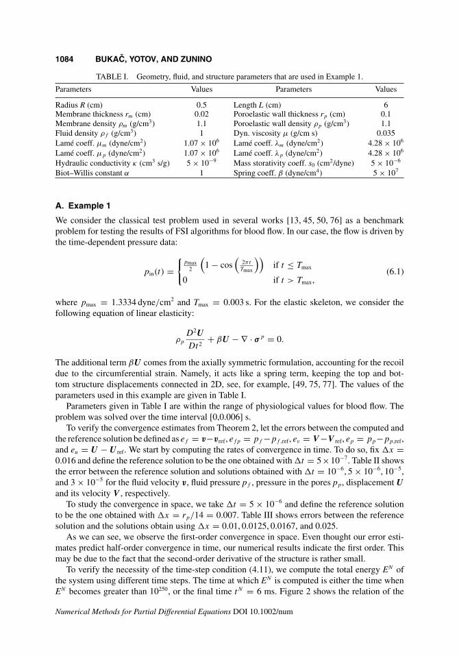
1084 BUKAC, YOTOV, AND ZUNINO
TABLE I. Geometry, fluid, and structure parameters that are used in Example 1.
Parameters Values Parameters Values
Radius R (cm) 0.5 Length L (cm) 6Membrane thickness rm (cm) 0.02 Poroelastic wall thickness rp (cm) 0.1Membrane density ρm (g/cm3) 1.1 Poroelastic wall density ρp (g/cm3) 1.1Fluid density ρf (g/cm3) 1 Dyn. viscosity μ (g/cm s) 0.035Lamé coeff. μm (dyne/cm2) 1.07 × 10⁶ Lamé coeff. λm (dyne/cm2) 4.28 × 10⁶
Lamé coeff. μp (dyne/cm2) 1.07 × 10⁶ Lamé coeff. λp (dyne/cm2) 4.28 × 10⁶
Hydraulic conductivity κ (cm3 s/g) 5 × 10⁻⁹ Mass storativity coeff. s0 (cm2/dyne) 5 × 10⁻⁶
Biot–Willis constant α 1 Spring coeff. β (dyne/cm4) 5 × 10⁷
A. Example 1
We consider the classical test problem used in several works [13, 45, 50, 76] as a benchmarkproblem for testing the results of FSI algorithms for blood flow. In our case, the flow is driven bythe time-dependent pressure data:
pin(t) ={
pmax2
(1 − cos
(2πt
Tmax
))if t ≤ Tmax
0 if t > Tmax,(6.1)
where pmax = 1.3334 dyne/cm2 and Tmax = 0.003 s. For the elastic skeleton, we consider thefollowing equation of linear elasticity:
ρp
D2U
Dt2+ βU − ∇ · σ p = 0.
The additional term βU comes from the axially symmetric formulation, accounting for the recoildue to the circumferential strain. Namely, it acts like a spring term, keeping the top and bot-tom structure displacements connected in 2D, see, for example, [49, 75, 77]. The values of theparameters used in this example are given in Table I.
Parameters given in Table I are within the range of physiological values for blood flow. Theproblem was solved over the time interval [0,0.006] s.
To verify the convergence estimates from Theorem 2, let the errors between the computed andthe reference solution be defined as ef = v−vref, efp = pf −pf ,ref, ev = V −V ref, ep = pp−pp,ref,and eu = U − U ref. We start by computing the rates of convergence in time. To do so, fix x =0.016 and define the reference solution to be the one obtained with t = 5×10⁻⁷. Table II showsthe error between the reference solution and solutions obtained with t = 10−6, 5 × 10⁻⁶, 10−5,and 3 × 10⁻⁵ for the fluid velocity v, fluid pressure pf , pressure in the pores pp, displacement U
and its velocity V , respectively.To study the convergence in space, we take t = 5 × 10⁻⁶ and define the reference solution
to be the one obtained with x = rp/14 = 0.007. Table III shows errors between the referencesolution and the solutions obtain using x = 0.01, 0.0125, 0.0167, and 0.025.
As we can see, we observe the first-order convergence in space. Even thought our error esti-mates predict half-order convergence in time, our numerical results indicate the first order. Thismay be due to the fact that the second-order derivative of the structure is rather small.
To verify the necessity of the time-step condition (4.11), we compute the total energy EN ofthe system using different time steps. The time at which EN is computed is either the time whenEN becomes greater than 10250, or the final time tN = 6 ms. Figure 2 shows the relation of the
Numerical Methods for Partial Differential Equations DOI 10.1002/num

TAB
LE
II.
Con
verg
ence
intim
e.
t
||ef|| l∞
(L2)
Rat
e||e
f|| l2
(H1)
Rat
e||e
fp|| l2
(L2)
Rat
e||e
v|| l∞
(L2)
Rat
e||e
p|| l∞
(L2)
Rat
e||e
p|| l2
(H1)
Rat
e||e
u|| l∞
(H1)
Rat
e
3×
10−5
7.6e
−1
–8.
8e−
2–
8.9e
−1
–3.
0e−
2–
6.3e
−1
–4.
1e−
1–
7.7e
−5
–10
−52.
7e−
10.
933.
1e−
20.
953.
4e−
10.
881.
0e−
20.
842.
2e−
10.
951.
5e−
10.
923.
0e−
50.
855
×10
−61.
3e−
11.
041.
5e−
21.
031.
6e−
11.
056.
0e−
30.
971.
1e−
11.
047.
4e−
21.
021.
5e−
50.
9710
−61.
5e−
21.
361.
8e−
31.
321.
8e−
21.
366.
9e−
41.
361.
2e−
21.
358.
5e−
31.
341.
8e−
61.
32

TAB
LE
III.
Con
verg
ence
insp
ace.
x
||ef|| l∞
(L2)
Rat
e||e
f|| l2
(H1)
Rat
e||e
fp|| l2
(L2)
Rat
e||e
v|| l∞
(L2)
Rat
e||e
p|| l∞
(L2)
Rat
e||e
p|| l2
(H1)
Rat
e||e
u|| l∞
(H1)
Rat
e
r p/4
2.4e
−1
–6.
8e−
1–
3.1e
−1
–2.
5e−
2–
1.2e
+0
–4.
0e−
1–
3.1e
−1
–r p
/5
1.9e
−1
1.01
6.2e
−1
0.43
2.6e
−1
0.83
1.8e
−2
1.46
0.9e
−1
0.92
3.6e
−1
0.47
2.6e
−1
0.84
r p/6
1.5e
−1
1.55
5.3e
−1
0.87
2.1e
−1
1.12
1.4e
−2
1.37
0.8e
−1
1.10
3.2e
−1
0.73
2.1e
−1
1.08
r p/7
1.2e
−1
1.37
4.5e
−1
1.06
1.7e
−1
1.32
1.0e
−2
1.6
0.6e
−1
1.34
2.7e
−1
1.01
1.8e
−1
1.08
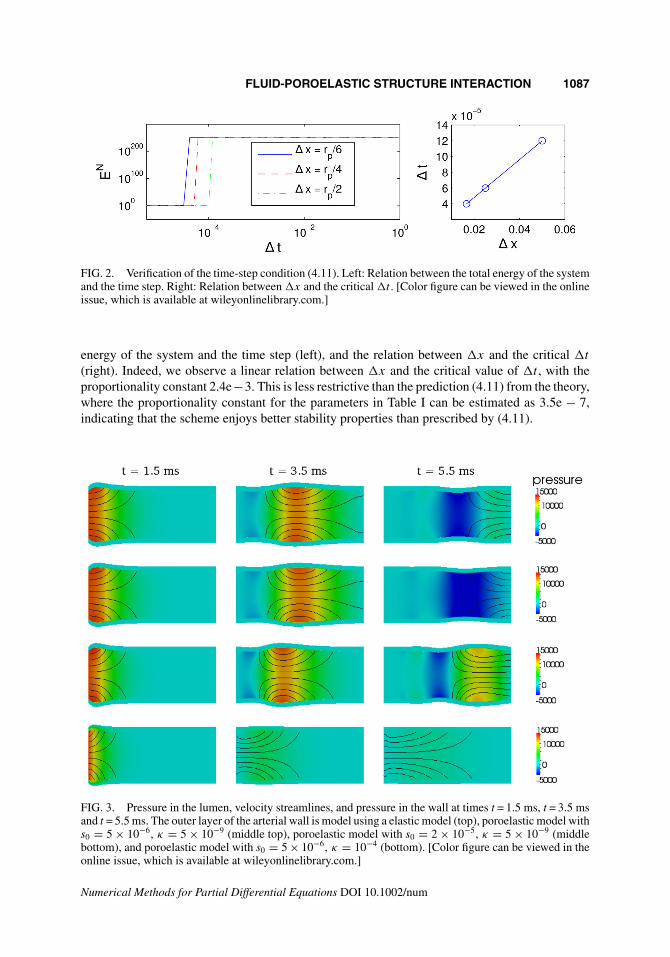
FLUID-POROELASTIC STRUCTURE INTERACTION 1087
FIG. 2. Verification of the time-step condition (4.11). Left: Relation between the total energy of the systemand the time step. Right: Relation between x and the critical t . [Color figure can be viewed in the onlineissue, which is available at wileyonlinelibrary.com.]
energy of the system and the time step (left), and the relation between x and the critical t
(right). Indeed, we observe a linear relation between x and the critical value of t , with theproportionality constant 2.4e−3. This is less restrictive than the prediction (4.11) from the theory,where the proportionality constant for the parameters in Table I can be estimated as 3.5e − 7,indicating that the scheme enjoys better stability properties than prescribed by (4.11).
FIG. 3. Pressure in the lumen, velocity streamlines, and pressure in the wall at times t = 1.5 ms, t = 3.5 msand t = 5.5 ms. The outer layer of the arterial wall is model using a elastic model (top), poroelastic model withs0 = 5 × 10⁻⁶, κ = 5 × 10⁻⁹ (middle top), poroelastic model with s0 = 2 × 10⁻⁵, κ = 5 × 10⁻⁹ (middlebottom), and poroelastic model with s0 = 5 × 10⁻⁶, κ = 10−4 (bottom). [Color figure can be viewed in theonline issue, which is available at wileyonlinelibrary.com.]
Numerical Methods for Partial Differential Equations DOI 10.1002/num

1088 BUKAC, YOTOV, AND ZUNINO
FIG. 4. Velocity magnitude at times t = 1.5 ms, t = 3.5 ms and t = 5.5 ms. The outer layer of the arterialwall is model using a elastic model (top), poroelastic model with s0 = 5 × 10⁻⁶, κ = 5 × 10⁻⁹ (middletop), poroelastic model with s0 = 2 × 10⁻⁵, κ = 5 × 10⁻⁹ (middle bottom), and poroelastic model withs0 = 5 × 10⁻⁶, κ = 10−4 (bottom). [Color figure can be viewed in the online issue, which is available atwileyonlinelibrary.com.]
B. Example 2
In this example, we compare our numerical results to the ones obtained using a purely elasticmodel for the outer layer of the arterial wall. More precisely, while the fluid and the membraneare modeled as before, we assume there is no fluid contained within the wall, and we model thethick wall using 2D linear elasticity
ρp
D2U
Dt2+ βU − ∇ · σE = 0; in �p(t) for t ∈ (0, T ).
The coupling conditions in this case are given as follows:
v = ξ , η = U on �(t), (6.2)
σ f n − σEn + J −1f = 0 on �(t). (6.3)
The problem is solved using an operator-splitting approach performed in the same spirit as inthis manuscript. The unconditional stability is due to the Robin boundary conditions that involvemembrane inertia, appearing in both fluid, and thick structure subproblems. For more details see[78].
For the purpose of understanding the poroelastic effects to the structure displacement, we distin-guish two cases: the high storativity case s0 � κ , and the high permeability case κ � s0. We give acomparison of the results obtained using the elastic model for the outer wall, and poroelastic model
Numerical Methods for Partial Differential Equations DOI 10.1002/num

FLUID-POROELASTIC STRUCTURE INTERACTION 1089
FIG. 5. From top to bottom: Flow rate, radial displacement of the membrane, mean pressure in the lumen,and mean pressure in the pores. Results were obtained using the elastic model (dotted line), and poro-elastic model with the following parameters: case 1 (s0 = 5 × 10⁻⁶, κ = 5 × 10⁻⁹; dashed line), case 2(s0 = 2 × 10⁻⁵, κ = 5 × 10⁻⁹; dash dot line), and case 3 (s0 = 5 × 10⁻⁶, κ = 1 × 10⁻⁴; solid line). [Colorfigure can be viewed in the online issue, which is available at wileyonlinelibrary.com.]
using two different values for s0, and two different values for κ . The first test case for the poroelas-tic wall will correspond to the parameters s0 and κ from Example 1 (s0 = 5×10⁻⁶, κ = 5×10⁻⁹),the second test case will correspond to the increased value of s0 (s0 = 2 × 10⁻⁵, κ = 5 × 10⁻⁹),and the third example to the increased value of κ (s0 = 5 × 10⁻⁶, κ = 10−4). Figure 3 shows thepressure pulse (colormap) and velocity streamlines obtained with the two models. The velocitymagnitude is shown in Fig. 4.
To quantify the differences, we compute average quantities on each vertical line Sri of the com-
putational mesh �r , corresponding to the position xi = i · x, where x = 0.016 and r ∈ {f , m}.The quantities of interest are membrane displacement, the mean pressure, and the flow rate in thelumen:
pf (xi) = 1
Sf
i
∫Sfi
pf ,hds, pp(xi) = 1
Sp
i
∫Spi
pp,hds, Q(xi) =∫
Sfi
vh · exds.
Figure 5 shows a comparison between the flow rate in the lumen, membrane displacement,and the mean pressure in the lumen and in the wall, obtained using a poroelastic model and anelastic model. In the high permeability regime, the structure displacement is the smallest, whilein this case, we observe the largest mean pressure in the wall. In the high storativity regime, weobserve a delay in the pressure wave propagation speed, and qualitatively different displacement.
Numerical Methods for Partial Differential Equations DOI 10.1002/num

1090 BUKAC, YOTOV, AND ZUNINO
VII. CONCLUSION
The focus of this article is on modeling and implementation of a fluid-poroelastic structure inter-action problem. In particular, we study the interaction between the fluid a multilayered wall, wherethe wall consists of a thin membrane, and a thick poroelastic medium. We proposed an explicitnumerical algorithm based on the Lie operator splitting scheme. An alternative discrete problemformulation based on Nitsche’s method for the enforcement of the interface conditions is understudy [79]. This new method can accommodate a mixed formulation for the Darcy’s equations.
We prove the conditional stability of the algorithm, and derive error estimates. Stability andconvergence results are validated by the numerical simulations. The drawback of the scheme isthat it requires pressure formulation for the Darcy equation. Concerning the application of thescheme to blood flow in arteries, we test numerically the porous effects in the wall, comparingresults obtained with different coefficients to the ones obtained using a purely elastic model. Weobserve different behavior depending on the storativity or permeability dominant regime.
APPENDIX AUXILIARY RESULTS
We collect in this section some auxiliary results and proofs that complement the stability andconvergence analysis of the proposed scheme. They are either a consequence of the standardtheory of the finite element method or they follow from basic results of approximation theory. Forthe reader’s convenience, we report them separately from the main body of the manuscript.
For any real numbers a, b, the following algebraic identities are satisfied:
(a − b)a = 1
2a2 − 1
2b2 + 1
2(a − b)2, (A1)
t
N−1∑n=0
an+1dtbn+1 = aNbN − t
N−1∑n=0
dtan+1bn − a0b0, (A2)
and for non-negative real numbers a, b, and ε > 0
ab ≤ a2
2ε+ εb2
2. (A3)
Lemma 2. Given the functional spaces Vf
h ⊂ V f , Qf
h ⊂ Qf , V p
h ⊂ V p, and Qp
h ⊂ Qp, thefollowing inequalities hold true:
• local trace-inverse inequality:
h||ψh||2L2(�)≤ CT I ||ψh||2L2(�p)
, ∀ψh ∈ Qp
h ; (A4)
• Cauchy-Schwarz inequality:∣∣∣∣∫
�f /p
v · udx
∣∣∣∣ ≤ ||v||L2(�f /p)||u||L2(�f /p) ∀v, u ∈ V f /p; (A5)
• Poincaré inequality:
||v||L2(�f /p) ≤ CPF ||∇v||L2(�f /p) ∀v ∈ V f /p; (A6)
Numerical Methods for Partial Differential Equations DOI 10.1002/num

FLUID-POROELASTIC STRUCTURE INTERACTION 1091
• trace inequality:
||v||L2(�) ≤ CT ||v||1/2
L2(�f /p)||∇v||1/2
L2(�f /p)∀v ∈ V f /p; (A7)
• Korn inequality:
||∇v||L2(�f /p) ≤ CK ||D(v)||L2(�f /p) ∀v ∈ V f /p. (A8)
Here, constants CPF , CT and CK depend on the domain �, and constant CT I depends on theangles in the finite element mesh.
Our analysis holds provided that the following regularity assumptions are satisfied by the exactsolution of the problem.
Assumption 1. Let X be a Banach space, and (0, T ) ⊂ R a time interval. We define the L2-spaceof functions u : (0, T ) → X by
L2(0, T ; X) ={u|u is measurable and
∫ T
0||u||2Xdt < ∞
},
and L∞-space by
L∞(0, T ; X) = {u|u is measurable and ||u||X is essentially bounded
}.
Then, the Sobolev space Wk,2(0, T ; X) = Hk(0, T ; X) is defined to be the set of all functionsu ∈ L2(0, T ; X) whose distributional time derivative Dα
t u belongs to L2(0, T ; X), for every α with|α| ≤ k. We assume that the weak solution of (2.28), complemented by the prescribed interface,boundary and initial conditions, is such that
v ∈ H 1(0, T ; Hk+1(�f )) ∩ H 2(0, T ; L2(�f )),
pf ∈ L2(0, T ; Hs+1(�f )),
η ∈ L∞(0, T ; Hk+1(0, L)) ∩ H 1(0, T ; Hk+1(0, L)) ∩ H 3(0, T ; L2(0, L)),
ξ ∈ H 2(0, T ; Hk+1(0, L)) ∩ H 3(0, T ; L2(0, L)),
∂tξ ∈ L∞(0, T ; Hk+1(0, L)),
∂ttξ ∈ L∞(0, T ; Hk+1(0, L)),
U ∈ L∞(0, T ; Hk+1(�p)) ∩ H 2(0, T ; Hk+1(�p)) ∩ H 3(0, T ; L2(�p)),
V ∈ L∞(0, T ; Hk+1(�p)) ∩ H 3(0, T ; L2(�p)),
∂tV ∈ L∞(0, T ; Hk+1(�p)),
∂ttV ∈ L∞(0, T ; Hk+1(�p)),
pp ∈ L∞(0, T ; Hk+1(�p)) ∩ H 1(0, T ; Hk+1(�p)) ∩ H 2(0, T ; L2(�p)). (A9)
Then, our finite element spaces satisfy the approximation properties reported below.
Lemma 3. Let Ph be the Lagrangian interpolation operator onto Vp
h , Ih = Ph|� be theLagrangian interpolation operator onto V m
h , Sh be a Stokes-like projection operator defined in
Numerical Methods for Partial Differential Equations DOI 10.1002/num

1092 BUKAC, YOTOV, AND ZUNINO
(5.5) , and let �f /p
h be the L2-orthogonal projections onto Qf /p
h defined in (5.1) . Using piecewisepolynomials of degree k and s, we have:
||v − Shv||H1(�f ) ≤ Chk||v||Hk+1(�f ), (A10)
||pf − �f
h pf ||L2(�f ) ≤ Chs+1||pf ||Hs+1(�f ), (A11)
||U − PhU ||L2(�p) ≤ Chk+1||U ||Hk+1(�p), (A12)
||U − PhU ||H1(�p) ≤ Chk||U ||Hk+1(�p), (A13)
||pp − �p
hpp||L2(�p) ≤ Chk+1||pp||Hk+1(�p), (A14)
||pp − �p
hpp||H1(�p) ≤ Chk||pp||Hk+1(�p). (A15)
Furthermore, since Ih = Ph|� is a Lagrangian interpolant, we have:
||U − PhU ||L2(�) = ||η − Ihη||L2(�) ≤ Chk+1||η||Hk+1(�), (A16)
||U − PhU ||H1(�) = ||η − Ihη||H1(�) ≤ Chk||η||Hk+1(�), (A17)
||V − PhV ||L2(�) = ||ξ − Ihξ ||L2(�) ≤ Chk+1||ξ ||Hk+1(�). (A18)
Proof. The proof of (A10) can be found in [15], Theorem B.5. For the proof of the otherinequalities, see [74].
Lemma 4 (Consistency and splitting errors). The following inequalities hold:
t
N−1∑n=0
||dtϕn+1 − ∂tϕ
n+1||2L2(�)
≤ C t2||∂ttϕ||2L2(0,T ;L2(�))
,
t
N−1∑n=1
||dttϕn+1 − ∂t (dtϕ
n+1)||2L2(�)
≤ C t2||∂tttϕ||2L2(0,T ;L2(�))
,
t2N−1∑n=0
||τ · σ f n + ρmrm
vn+1 · τ − V n · τ
t||2
L2(�)≤ C t ||η||2
l2(0,T ;H2(0,L))
+ C t3||∂ttv · τ ||2L2(0,T ;L2(�))
t
N−1∑n=0
||∇(ϕn+1 − ϕn)||2L2(�)
≤ C t2||∂tϕ||2L2(0,T ;H1(�))
,
t
N−1∑n=0
||∇(dtϕn+1 − ∂tϕ
n+1)||2L2(�)
≤ C t2||∂ttϕ||2L2(0,T ;H1(�))
,
||dtϕN − ∂tϕ
N ||2L2(�)
≤ t2max0≤n≤N ||∂ttϕn||2
L2(�)= t2||∂ttϕ||2
l∞(0,T ;L2(�)),
Proof. We will prove the first three inequalities. The proofs for other inequalities are similar.Using Cauchy–Schwartz inequality, we have
t
N−1∑n=0
||dtϕn+1 − ∂tϕ
n+1||2L2(�)
= t
N−1∑n=0
∫�
∣∣∣∣ 1
t
∫ tn+1
tn(t − tn)∂ttϕ(t)dt
∣∣∣∣2
dx
Numerical Methods for Partial Differential Equations DOI 10.1002/num

FLUID-POROELASTIC STRUCTURE INTERACTION 1093
≤ 1
t
∫�
N−1∑n=0
(∫ tn+1
tn|t − tn|2dt
∫ tn+1
tn|∂ttϕ|2dt
)dx ≤ C t2
∫�
∫ T
0|∂ttϕ|2dtdx
≤ C t2||ϕ||2L2(0,T ;L2(�)).
To prove the next two inequalities, we integrate by parts twice, and use Cauchy–Schwartzinequality:
t
N−1∑n=1
||dttϕn+1 − ∂t (dtϕ
n+1)||2L2(�)
= t
N−1∑n=0
∣∣∣∣∣∣∣∣ 1
t2
( ∫ tn+1
tn(t − tn)∂ttϕdt +
∫ tn−1
tn(t − tn−1)∂ttϕdt
)∣∣∣∣∣∣∣∣2
L2(�)
= 1
t3
N−1∑n=0
∣∣∣∣∣∣∣∣(
t2
2
∫ tn+1
tn∂tttϕdt−
∫ tn+1
tn
(t − tn)2
2∂tttϕdt−
∫ tn−1
tn
(t − tn−1)2
2∂tttϕdt
)∣∣∣∣∣∣∣∣2
L2(�)
≤ 1
t3
∫�
N−1∑n=0
( t4
4
∣∣∣∣∫ tn+1
tn∂tttϕdt
∣∣∣∣2
+∣∣∣∣∫ tn+1
tn
(t − tn)2
2∂tttϕdt
∣∣∣∣2
+∣∣∣∣∫ tn−1
tn
(t − tn−1)2
2∂tttϕdt
∣∣∣∣2)
dx
≤ 1
t3
∫�
N−1∑n=0
( t5
4
∫ tn+1
tn|∂tttϕ|2dt + t5
10
∫ tn+1
tn|∂tttϕ|2dt + t5
10
∫ tn−1
tn|∂tttϕ|2dt
)dx
≤ C t2||∂tttϕ||2L2(0,T ;L2(�))
To prove the third inequality, note that V n · τ = vn · τ on �, since V n and vn are solutions tothe continuous problem. Thus, since the exact solution satisfies Eq. (2.22), we have
t2N−1∑n=0
∣∣∣∣∣∣∣∣τ · σ f n + ρmrm
vn+1 · τ − vn · τ
t
∣∣∣∣∣∣∣∣2
L2(�)
= t2N−1∑n=0
||τ · σ f n + ρmrmdtvn+1 · τ ||2
L2(�)
= t2N−1∑n=0
||τ · Lη + τ · σ pn + ρmrm(dtvn+1 · τ − ∂tv
n+1 · τ )||2L2(�)
≤ C t2N−1∑n=0
||ηn+1||2H2(0,L)
+ C t2N−1∑n=0
||dtvn+1 · τ − ∂tv
n+1 · τ ||2L2(�)
≤ C t ||η||2l2(0,T ;H2(0,L))
+ C t3||∂ttv · τ ||2L2(0,T ;L2(�))
.
Lemma 5. The following estimate holds:
t
N−1∑n=0
(Rn+1f (δn+1
f ) + Rn+1s (dt δ
n+1u ) + Rn+1
v (dt δn+1v ) + Rn+1
p (δn+1p ) + Rn+1
os1 (δn+1f ) + Rn+1
os2 (δn+1f − dt δ
n+1u ))
Numerical Methods for Partial Differential Equations DOI 10.1002/num
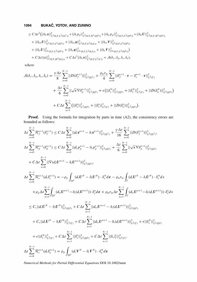
1094 BUKAC, YOTOV, AND ZUNINO
≤ C t2(||∂ttv||2
L2(0,T ;L2(�f ))+||∂tpp||2
L2(0,T ;H1(�p))+||∂ttpp||2
L2(0,T ;L2(�p))+||∂ttU ||2
L2(0,T ;H1(�p))
+ ||∂tttU ||2L2(0,T ;L2(�p))
+ ||∂tttη||2L2(0,T ;L2(0,L))
+ ||∂tttV ||2L2(0,T ;L2(�p))
+ ||∂ttU ||2l∞(0,T ;L2(�p))
+ ||∂ttη||2l∞(0,T ;L2(0,L))
+ ||∂ttV ||2l∞(0,T ;L2(�p))
)+ C t ||η||2
l2(0,T ;H2(0,L))+ C t3||∂ttv||2
L2(0,T ;L2(�))+ A(δf , δp , δv , δu),
where
A(δf , δp, δv , δu) = γ t
8
N−1∑n=0
||D(δn+1f )||2
L2(�f )+ ρmrm
4
N−1∑n=0
||δn+1f · τ − δn+1
v · τ ||2L2(�)
+ t
6
N−1∑n=0
||√κ∇δn+1p ||2
L2(�p)+ ε
(||δNv ||2
L2(�p)+ ||δN
v ||2L2(�)
+ ||D(δNu )||2
L2(�p)
)
+ C t
N−1∑n=1
(||δnv ||2L2(�p)
+ ||δnv ||2L2(�)
+ ||D(δnu)||2L2(�p)
).
Proof. Using the formula for integration by parts in time (A2), the consistency errors arebounded as follows:
t
N−1∑n=0
Rn+1f (δn+1
f ) ≤ C t
N−1∑n=0
||dtvn+1 − ∂tv
n+1||2L2(�f )
+ γ t
16
N−1∑n=0
||D(δn+1f )||2
L2(�f ),
t
N−1∑n=0
Rn+1p (δn+1
p ) ≤ C t
N−1∑n=0
||dtpn+1p − ∂tp
n+1p ||2
L2(�p)+ t
6
N−1∑n=0
||√κ∇δn+1p ||2
L2(�p)
+ C t
N−1∑n=0
||∇(dtUn+1 − ∂tU
n+1)||2L2(�p)
,
t
N−1∑n=0
Rn+1v (dtδ
n+1v ) = −ρp
∫�p
(dtUN − ∂tU
N) · δNv dx − ρmrm
∫�
(dtUN − ∂tU
N) · δNv dx
+ρp t
N−1∑n=1
∫�p
(dttUn+1−∂t (dtU
n+1))·δnvdx + ρmrm t
N−1∑n=1
∫�
(dttUn+1−∂t (dtU
n+1))·δnvdx
≤ Cε||dtUN − ∂tU
N ||2L2(�p)
+ C t
N−1∑n=1
||dttUn+1 − ∂t (dtU
n+1)||2L2(�p)
+ Cε||dtUN − ∂tU
N ||2L2(�)
+ C t
N−1∑n=1
||dttUn+1 − ∂t (dtU
n+1)||2L2(�)
+ ε||δNv ||2
L2(�p)
+ ε||δNv ||2
L2(�)+ C t
N−1∑n=1
||δnv ||2L2(�p)
+ C t
N−1∑n=1
||δv|n�||2L2(�)
.
t
N−1∑n=0
Rn+1s (dtδ
n+1u ) = ρp
∫�p
(dtVN − ∂tV
N) · δNu dx
Numerical Methods for Partial Differential Equations DOI 10.1002/num

FLUID-POROELASTIC STRUCTURE INTERACTION 1095
− ρp t
N−1∑n=1
∫�p
(dttVn+1 − ∂t (dtV
n+1)) · δnudx ≤ Cε||dtV
N − ∂tVN ||2
L2(�p)
+ C t
N−1∑n=1
||dttVn+1 − ∂t (dtV
n+1)||2L2(�p)
+ ε||D(δNu )||2
L2(�p)
+ C t
N−1∑n=1
||D(δnu)||2L2(�p)
t
N−1∑n=0
Rn+1os1 (δn+1
f ) ≤ C t
N−1∑n=0
||∇(pn+1p − pn
p)||2L2(�p)
+ γ t
16
N−1∑n=0
||D(δn+1f )||2
L2(�f ), t
N−1∑n=0
Ros(δn+1f − dtδ
n+1u ) = t
N−1∑n=0
∫�
×(
τ · σ f n + ρmrm
vn+1 · τ − V n · τ
t
)(δn+1
f · τ − δn+1v · τ )dx
≤ t2
ρmrm
N−1∑n=0
∣∣∣∣∣∣∣∣τ · σ f n + ρmrm
vn+1 · τ − V n · τ
t
∣∣∣∣∣∣∣∣2
L2(�)
+ ρmrm
4
N−1∑n=0
||δn+1f · τ − δn+1
v · τ ||2L2(�)
.
The final consistency error estimate follows by applying Lemma 4.
Lemma 6. (Interpolation errors). The following inequalities hold:
t
N−1∑n=0
||dtθn+1p ||2
L2(�p)≤ ||∂tθ
np ||2
L2(0,T ;L2(�p))≤ h2k+2||∂tpp||2L2(0,T ;Hk+1(�p))
,
t
N−1∑n=0
||∇dtθn+1f ||2
L2(�f )≤ ||∂tθf ||2
L2(0,T ;H1(�f ))≤ h2k||∂tv||2
L2(0,T ;Hk+1(�f )),
t
N−1∑n=0
||dtt θn+1s ||2
L2(�p)≤ ||∂tt θs ||2L2(0,T ;L2(�p))
≤ h2k+2||∂ttU ||2L2(0,T ;Hk+1(�p))
,
t
N−1∑n=0
||dtθn+1v ||2
L2(�)≤ ||∂tθv||2L2(0,T ;L2(�))
≤ h2k+2||∂tξ ||2L2(0,T ;Hk+1(0,L)
,
t
N−1∑n=0
||dtθs |n+1� ||2M ≤ ||∂tθs |�||2
L2(0,T ;H1(0,L))≤ h2k||∂tη||2
L2(0,T ;Hk+1(0,L)),
t
N−1∑n=0
(||D(θn+1f )||2
L2(�f )+ ||∇θn+1
p ||2L2(�p)
+ ||∇θnp ||2
L2(�p)
)
≤ t
N∑n=0
h2k(||vn||2
Hk+1(�f )+ ||pn
p||2Hk+1(�p)
)≤ h2k
(||v||2l2(0,T ;Hk+1(�f ))
+ ||pp||2l2(0,T ;Hk+1(�p))
).
max0≤n≤N
||dtθnv ||2
L2(�p)≤ C
(h2k+2||∂tV ||2
l∞(0,T ;Hk+1(�p))+ h2k+4||∂ttV ||2
l∞(0,T ;Hk+1(�p))
),
Numerical Methods for Partial Differential Equations DOI 10.1002/num

1096 BUKAC, YOTOV, AND ZUNINO
Proof. We only give the proof for the last inequality in Lemma 6. Other inequalities can beeasily shown using manipulations similar to the ones in Lemma 5, and approximation properties(A10)–(A15).
From Taylor expansion, we have
dtθnv = ∂tθ
nv + t
2∂tt θv(z), z ∈ [tn, tn+1].
Using the equality above, we get the following
max0≤n≤N
||dtθnv ||2
L2(�p)= max
0≤n≤N
∥∥∥∥∂tθnv + t
2∂tt θv(z)
∥∥∥∥2
L2(�p)
≤ C(h2k+2||∂tV ||2
l∞(0,T ;Hk+1(�p))+ t2h2k+2||∂ttV ||2
l∞(0,T ;Hk+1(�p))
)≤ C
(h2k+2||∂tV ||2
l∞(0,T ;Hk+1(�p))+ h2k+4||∂ttV ||2
l∞(0,T ;Hk+1(�p))
).
The last inequality is obtained using the CFL condition (4.11).
References
1. Y. Cao, M. Gunzburger, X. Hu, F. Hua, X. Wang, and W. Zhao, Finite element approximationsfor Stokes-Darcy flow with Beavers-Joseph interface conditions, SIAM J Numer Anal 47 (2010),4239–4256.
2. M. Discacciati, E. Miglio, and A. Quarteroni, Mathematical and numerical models for coupling surfaceand groundwater flows, Appl Numer Math 43 (2002), 57–74.
3. M. Discacciati, A. Quarteroni, and A. Valli, Robin-Robin domain decomposition methods for theStokes-Darcy coupling, SIAM J Numer Anal 45 (2007), 1246–1268.
4. V. Girault and B. Rivière, DG approximation of coupled Navier-Stokes and Darcy equations byBeaver-Joseph-Saffman interface condition, SIAM J Numer Anal 47 (2009), 2052–2089.
5. W. Layton, F. Schieweck, and I. Yotov, Coupling fluid flow with porous media flow, SIAM J NumerAnal 40 (2002), 2195–2218.
6. W. Layton, H. Tran, and X. Xiong, Long time stability of four methods for splitting the evolution-ary Stokes–Darcy problem into Stokes and Darcy subproblems, J Comput Appl Math 236 (2012),3198–3217.
7. M. Mu and J. Xu, A two-grid method of a mixed Stokes-Darcy model for coupling fluid flow with porousmedia flow, SIAM J Numer Anal 45 (2007), 1801–1813.
8. M. Mu and X. Zhu, Decoupled schemes for a non-stationary mixed Stokes-Darcy model, Math Comput79 (2010), 707–731.
9. B. Rivière and I. Yotov, Locally conservative coupling of Stokes and Darcy flows, SIAM J Numer Anal42 (2005), 1959–1977.
10. P. Song, C. Wang, and I. Yotov, Domain decomposition for Stokes-Darcy flows with curved interfaces,Proc Comput Sci 18 (2013), 1077–1086.
11. S. Badia, F. Nobile, and C. Vergara, Robin-Robin preconditioned Krylov methods for fluid-structureinteraction problems, Comput Methods Appl Mech Eng 198 (2009), 2768–2784.
12. S. Badia, A. Quaini, and A. Quarteroni, Coupling Biot and Navier–Stokes equations for modellingfluid–poroelastic media interaction, J Comput Phys 228 (2009), 7986–8014.
Numerical Methods for Partial Differential Equations DOI 10.1002/num

FLUID-POROELASTIC STRUCTURE INTERACTION 1097
13. M. Bukac, S. Canic, R. Glowinski, J. Tambaca, and A. Quaini, Fluid-structure interaction inblood flow capturing non-zero longitudinal structure displacement, J Comput Phys 235 (2012),515–541.
14. M. A. Fernández and M. Landajuela, A fully decoupled scheme for the interaction of a thin-walledstructure with an incompressible fluid, C R Math 351 (2013), 161–164.
15. M. A. Fernández, Incremental displacement-correction schemes for incompressible fluid-structureinteraction: stability and convergence analysis, Numer Math 123 (2012), 210–65.
16. P. Hansbo, Nitsche’s method for interface problems in computational mechanics, GAMM Mitt 28 (2005),183–206.
17. M. Lukácová-Medvid’ová, G. Rusnáková, and A. Hundertmark-Zaušková, Kinematic splitting algo-rithm for fluid-structure interaction in hemodynamics, Comput Methods Appl Mech Eng 265 (2013),83–106.
18. B. Muha and S. Canic, Existence of a solution to a fluid-multi-layered-structure interaction problem, JDifferential Equations 256 (2014), 658–706.
19. F. Nobile and C. Vergara, An effective fluid-structure interaction formulation for vascular dynamics bygeneralized Robin conditions, SIAM J Sci Comput 30 (2008), 731–763.
20. A. Quaini and A. Quarteroni, A semi-implicit approach for fluid-structure interaction based on analgebraic fractional step method, Math Models Methods Appl Sci 17 (2007), 957–985.
21. P. Causin, J. F. Gerbeau, and F. Nobile, Added-mass effect in the design of partitioned algorithms forfluid-structure problems, Comput Methods Appl Mech Eng 194 (2005), 4506–4527.
22. R. L. Armentano, J. G. Barra, J. Levenson, A. Simon, and R. H. Pichel, Arterial wall mechanics inconscious dogs: Assessment of viscous, inertial, and elastic moduli to characterize aortic wall behavior,Circ Res 76 (1995), 468–478.
23. R. D. Bauer, R. Busse, A. Schabert, Y. Summa, and E. Wetterer, Separate determination of thepulsatile elastic and viscous forces developed in the arterial wall in vivo, Pflügers Arch 380 (1976),221–226.
24. S. Canic, J. Tambaca, G. Guidoboni, A. Mikelic, C.J. Hartley, and D. Rosenstrauch, Modeling vis-coelastic behavior of arterial walls and their interaction with pulsatile blood flow, SIAM J Appl Math67 (2006), 164–193.
25. Y. C. Fung, Biomechanics: its foundation and objectives, Y. C. Fung, N. Perrone, and M. Anliker, editors,Prentice-Hall, Englewood Cliff, NJ, 1972.
26. J. D. Humphrey et al., Mechanics of the arterial wall: review and directions, Crit Rev Biomed Eng 23(1995), 1.
27. A. Robertson, M. Hill, and D. Li, Structurally motivated damage models for arterial walls, Theory andapplication, Modeling of physiological flows, Springer Milan, 2012, pp. 143–185.
28. R. Vito and S. Dixon, Blood vessel constitutive models-1995–2002, Annu Rev Biomed Eng 5 (2003),413–439.
29. J. Zhou and Y. C. Fung, The degree of nonlinearity and anisotropy of blood vessel elasticity, Proc NatlAcad Sci USA 94 (1997), 14255–14260.
30. M. Prosi, P. Zunino, K. Perktold, and A. Quarteroni, Mathematical and numerical models for transferof low-density lipoproteins through the arterial walls: a new methodology for the model set up withapplications to the study of disturbed lumenal flow, J Biomech 38 (2005), 903–917.
31. M. Lesinigo, Lumped mathematical models for intracranial dynamics, Ph.D. thesis, EPFL, Switzerland,2013.
32. G. A. Holzapfel and R. W. Ogden, Constitutive modelling of passive myocardium: a structurallybased framework for material characterization, Philos Trans R Soc A Math Phys Eng Sci 367 (2009),3445–3475.
Numerical Methods for Partial Differential Equations DOI 10.1002/num

1098 BUKAC, YOTOV, AND ZUNINO
33. G. A. Holzapfel, G. Sommer, and P. Regitnig, Anisotropic mechanical properties of tissue componentsin human atherosclerotic plaques, Trans ASME K J Biomech Eng 126 (2004), 657–665.
34. S. M. K. Rausch, C. Martin, P. B. Bornemann, S. Uhlig, and W. A. Wall, Material model of lungparenchyma based on living precision-cut lung slice testing, J Mech Behav Biomed Mater 4 (2011),583–592.
35. D. Tang, C. Yang, T. Geva, G. Gaudette, and P. Del Nido, Multi-physics MRI-based two-layerfluid–structure interaction anisotropic models of human right and left ventricles with different patchmaterials: cardiac function assessment and mechanical stress analysis, Comput Struct 89 (2011),1059–1068.
36. J.-M. Kim, S.-H. Chang, and C.-B. Yun, Fluid-structure-soil interaction analysis of cylindrical liq-uid storage tanks subjected to horizontal earthquake loading, Struct Eng Mech 13 (2002), 615–638.
37. N. D. Botkin, K.-H. Hoffmann, O. A. Pykhteev, and V. L. Turova, Dispersion relations for acousticwaves in heterogeneous multi-layered structures contacting with fluids, J Franklin Inst 344 (2007),520–534.
38. S. Chung and K. Vafai, Effect of the fluid–structure interactions on low-density lipoprotein transportwithin a multi-layered arterial wall, J Biomech 45 (2012), 371–381.
39. K. Lee, G. M. Saidel, and M. S. Penn, Permeability change of arterial endothelium is an age-dependentfunction of lesion size in apolipoprotein e-null mice, Am J Physiol Heart Circ Physiol 295 (2008),H2273–H2279.
40. M. Bukac, I. Yotov, R. Zakerzadeh, and P. Zunino, Effects of poroelasticity on fluid - structure interactionin arteries: a computational sensitivity studyModeling the heart and the circulatory system, in SpringerSeries in Modeling, Simulation and Applications (MS&A), Vol. 13, to appear.
41. N. Koshiba, J. Ando, X. Chen, and T. Hisada, Multiphysics simulation of blood flow and LDL transportin a porohyperelastic arterial wall model, J Biomech Eng 129 (2007), 374–385.
42. M. A. Murad, J. N. Guerreiro, and A. F. D. Loula, Micromechanical computational modeling of sec-ondary consolidation and hereditary creep in soils, Comput Methods Appl Mech Eng 190 (2001),1985–2016.
43. R. Showalter, Poroelastic filtration coupled to Stokes flow, Lect Notes Pure Appl Math 242 (2010),229–241.
44. B. Tully and Y. Ventikos, Coupling poroelasticity and CFD for cerebrospinal fluid hydrodynamics, IEEETrans Biomed Eng 56 (2009), 1644–1651.
45. S. Badia, F. Nobile, and C. Vergara, Fluid-structure partitioned procedures based on Robin transmissionconditions, J Comput Phys 227 (2008), 7027–7051.
46. C. Förster, W. Wall, and E. Ramm, Artificial added mass instabilities in sequential staggered coupling ofnonlinear structures and incompressible viscous flows, Comput Methods Appl Mech Eng 196 (2007),1278–1293.
47. M. Astorino, F. Chouly, and M. A. Fernández, An added-mass free semi-implicit coupling scheme forfluid-structure interaction, C R Math 347 (2009), 99–104.
48. M. Astorino, F. Chouly, and M. A. Fernández Varela, Robin based semi-implicit couplingin fluid-structure interaction: stability analysis and numerics. SIAM J Sci Comput 31 (2009),4041–4065.
49. S. Badia, A. Quaini, and A. Quarteroni, Splitting methods based on algebraic factorization forfluid-structure interaction, SIAM J Sci Comput 30 (2008), 1778–1805.
50. E. Burman and M. A. Fernández, Stabilization of explicit coupling in fluid-structure interaction involvingfluid incompressibility, Comput Methods Appl Mech Eng 198 (2009), 766–784.
51. S. Deparis, M. Discacciati, G. Fourestey, and A. Quarteroni, Fluid-structure algorithms based onSteklov-Poincaré operators, Comput Methods Appl Mech Eng 195 (2006), 5797–5812.
Numerical Methods for Partial Differential Equations DOI 10.1002/num

FLUID-POROELASTIC STRUCTURE INTERACTION 1099
52. S. Deparis, M. Fernandez, and L. Formaggia, Acceleration of a fixed point algorithm for a fluid-structureinteraction using transpiration condition, Math Model Numer Anal 37 (2003), 601–616.
53. M. A. Fernández, Incremental displacement-correction schemes for the explicit coupling of a thinstructure with an incompressible fluid, C R Math 349 (2011), 473–477.
54. M. A. Fernández, J. F. Gerbeau, and C. Grandmont, A projection algorithm for fluid-structure interactionproblems with strong added-mass effect, C R Math 342 (2006), 279–284.
55. M. A. Fernández and J. Mullaert, Displacement-velocity correction schemes for incompressiblefluid-structure interaction, C R Math Acad Sci Paris 349 (2011), 1011–1015.
56. G. Guidoboni, R. Glowinski, N. Cavallini, and S. Canic, Stable loosely-coupled-type algorithm forfluid-structure interaction in blood flow, J Comput Phys 228 (2009), 6916–6937.
57. C. M. Murea and S. Sy, A fast method for solving fluid-structure interaction problems numerically, IntJ Numer Methods Fluids 60 (2009), 1149–1172.
58. L. Gerardo-Giorda, F. Nobile, and C. Vergara, Analysis and optimization of Robin-Robin partitionedprocedures in fluid-structure interaction problems, SIAM J Numer Anal 48 (2010), 2091–2116.
59. E. Burman and M. A. Fernández, An unfitted Nitsche method for incompressible fluid-structure inter-action using overlapping meshes, Comput Methods Appl Mech Eng, DOI: 10.1016/j.cma.2014.07.007,(2014).
60. R. Glowinski, Finite element methods for incompressible viscous flow, P. G. Ciarlet and J.-L. Lions,editors, Handbook of numerical analysis, Vol. 9, North-Holland, Amsterdam, The Netherlands, 2003.
61. B. Muha and S. Canic, Existence of a weak solution to a nonlinear fluid–structure interaction problemmodeling the flow of an incompressible, viscous fluid in a cylinder with deformable walls, Arch RationMech Anal 207 (2013), 919–968.
62. A. Hundertmark-Zaušková, M. Lukácová-Medvid’ová, and G. Rusnáková, Fluid-structure interactionfor shear-dependent non-Newtonian fluids, Topics in mathematical modeling and analysis, Volume 7of Jindrich Necas Center for Mathematical Modeling Lecture Notes, Matfyzpress, Prague, 2012, pp.109–158.
63. L. Shan, H. Zheng, and W. Layton, A decoupling method with different subdomain time steps for thenonstationary Stokes–Darcy model, Numer Methods Partial Differential Equations 29 (2013), 549–583.
64. L. A. Miller and C. S. Peskin, A computational fluid dynamics of ‘clap and fling’ in the smallest insects,J Exp Biol 208 (2005), 195–212.
65. F. Nobile, Numerical approximation of fluidstructure interaction problems with application to haemo-dynamics, Ph.D. thesis, EPFL, Switzerland, 2001.
66. I. E. Vignon-Clementel, C. Alberto Figueroa, K. E. Jansen, and C. A. Taylor, Outflow boundary con-ditions for three-dimensional finite element modeling of blood flow and pressure in arteries, ComputMethods Appl Mech Eng 195 (2006), 3776–3796.
67. F. Nobile, M. Pozzoli, and C. Vergara, Time accurate partitioned algorithms for the solution offluid-structure interaction problems in haemodynamics, Comput Fluids 86 (2013), 470–482.
68. P. Moireau, N. Xiao, M. Astorino, A. Figueroa, D. Chapelle, C. Taylor, and J.-F. Gerbeau, Externaltissue support and fluid–structure simulation in blood flows, Biomech Model Mechanobiol 11 (2012),1–18.
69. P. Crosetto, S. Deparis, G. Fourestey, and A. Quarteroni, Parallel algorithms for fluid-structure interactionproblems in haemodynamics, SIAM J Sci Comput 33 (2011), 1598–1622.
70. E. Detournay and A. H. D. Cheng, Fundamentals of poroelasticity, Chapter 5 in Comprehensive rockengineering: principles, practice and projects, Vol. II, C. Fairhurst, editor, Analysis and design method,Pergamon Press, 1993, pp. 113–171.
71. J. Donea, Arbitrary Lagrangian-Eulerian finite element methods, Computational methods for transientanalysis, North-Holland, Amsterdam, The Netherlands, 1983.
Numerical Methods for Partial Differential Equations DOI 10.1002/num

1100 BUKAC, YOTOV, AND ZUNINO
72. T. J. R. Hughes, W. K. Liu, and T. K. Zimmermann, Lagrangian-Eulerian finite element formulation forincompressible viscous flows, Comput Methods Appl Mech Eng 29 (1981), 329–349.
73. A. Mikelic and M. Wheeler, Convergence of iterative coupling for coupled flow and geomechanics,Comput Geosci 17 (2013), 1–7.
74. P. Ciarlet, The finite element method for elliptic problems, Vol. 4, North Holland, 1978.
75. A. T. Barker and X. C. Cai, Scalable parallel methods for monolithic coupling in fluid-structureinteraction with application to blood flow modeling, J Comput Phys 229 (2010), 642–659.
76. L. Formaggia, J.F. Gerbeau, F. Nobile, and A. Quarteroni, On the coupling of 3D and 1D Navier–Stokesequations for flow problems in compliant vessels, Comput Methods Appl Mech Eng 191 (2001),561–582.
77. X. Ma, G. C. Lee, and S. G. Wu, Numerical simulation for the propagation of nonlinear pulsatile wavesin arteries, J Biomech Eng 114 (1992), 490.
78. M. Bukac, S. Canic, and B. Muha, A partitioned scheme for fluid-composite structure interactionproblems, Submitted, arXiv:1402.0110, J Comp Phys, doi: 10.1016/j.jcp.2014.10.045 (2014).
79. M. Bukac, I. Yotov, R. Zakerzadeh, and P. Zunino, Partitioning strategies for the interaction of a fluidwith a poroelastic material based on a Nitsche’s coupling approach, Submitted.
Numerical Methods for Partial Differential Equations DOI 10.1002/num