An Open Source Inertial Sensor Network with Bluetooth Smart

by

Hao Yan

A thesis submitted in conformity with the requirements for the degree of Master of Applied Science

Department of Electrical and Computer Engineering

University of Toronto

© Copyright by Hao Yan, 2014

ii

An Open Source Inertial Sensor Network with Bluetooth Smart

Hao Yan

Master of Applied Science

Department of Electrical and Computer Engineering

University of Toronto

2014

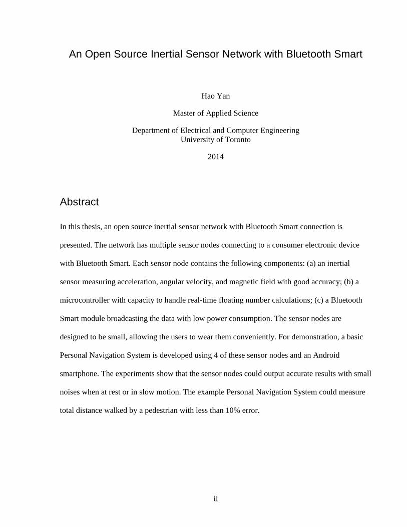
Abstract

In this thesis, an open source inertial sensor network with Bluetooth Smart connection is

presented. The network has multiple sensor nodes connecting to a consumer electronic device

with Bluetooth Smart. Each sensor node contains the following components: (a) an inertial

sensor measuring acceleration, angular velocity, and magnetic field with good accuracy; (b) a

microcontroller with capacity to handle real-time floating number calculations; (c) a Bluetooth

Smart module broadcasting the data with low power consumption. The sensor nodes are

designed to be small, allowing the users to wear them conveniently. For demonstration, a basic

Personal Navigation System is developed using 4 of these sensor nodes and an Android

smartphone. The experiments show that the sensor nodes could output accurate results with small

noises when at rest or in slow motion. The example Personal Navigation System could measure

total distance walked by a pedestrian with less than 10% error.

iii

Acknowledgments

I wish to express my gratitude to my supervisor, Professor David A. Johns, for his patient

guidance and encouragement throughout my time as his student. Professor Johns has offered me

inspiring advices from choosing the thesis subject to writing the thesis. I would not be able to

overcome some obstacles during the project without his unreserved assistance.

I would like to thank Dr. Chuhong Fei and Dr. Zhiyun Lin for devoting time to read my

manuscript and providing me with significant and constructive suggestions. Their valuable input

helps me enormously.

Thanks to Fengmin Gong from Zhejiang University for guiding me on PCB board design and

manufacture. Without his kind assistance, I would not be able to finish the prototype board in

time.

Finally I would like to thank my family for their continuous support since my undergraduate

years. I would like to thank my father especially for discussions on debugging issues of the

project.

iv

Table of Contents

Acknowledgments iii

Table of Contents iv

List of Tables viii

List of Figures ix

List of Acronyms xi

Chapter 1: Introduction 1

1.1 Introduction to inertial sensor networks 1

1.2 Applications of inertial sensor networks 2

1.3 Motivation 4

1.4 Thesis outline 5

Chapter 2: Background 6

2.1 Inertial measurement units 6

2.2 Wireless communication protocols 7

2.2.1 Wi-Fi and Wi-Fi Direct 8

2.2.2 ZigBee 8

2.2.3 Bluetooth 9

2.2.4 Bluetooth Smart 9

2.3 Wearable body sensor networks 10

v

2.4 Personal navigation systems 12

Chapter 3: Implementation of Sensor Node 15

3.1 Overall architecture of a sensor node 15

3.1.1 Power 17

3.1.2 Clocking 18

3.1.3 Programming interface 19

3.1.4 Unit cost 19

3.1.5 Physical size 20

3.2 Hardware implementation 20

3.2.1 Microcontroller: TM4C123GH6PM 20

3.2.2 Motion sensor: MPU9150 22

3.2.3 Bluetooth Smart module: BLE113 24

3.3 Microcontroller software Design 25

3.3.1 Initialization and configuration 25

3.3.2 Data and control flow 31

3.3.3 Implementation of BGLib 32

3.3.4 Simple calibration 36

3.4 Bluetooth Smart module configuration 38

3.4.1 Configurations in hardware.xml 38

3.4.2 Configurations in gatt.xml 39

vi

Chapter 4: Application Example – Personal Navigation System 41

4.1 How to determine the current step length 43

4.2 How to differentiate between steps 46

4.3 Android app design 48

Chapter 5: Experiments and Results 50

5.1 Performance of individual sensor node 50

5.1.1 Data accuracy at rest 50

5.1.2 Data accuracy while moving 58

5.1.3 Data rate limitation for BLE 64

5.1.4 Battery Life 66

5.2 Performance of inertial sensor network 66

5.3 Results of MotionTracker PNS 67

Chapter 6: Conclusion and Future Work 71

6.1 Conclusions 71

6.2 Future work on the inertial sensor network 73

Reference 75

Appendices 78

A. Cost of components for a sensor node 78

B. Source code for sensor node software 80

C. Source code for MotionTracker app 81

vii

D. Schematics and PCB design files for the sensor node board 82

viii

List of Tables

Table 1: Possible applications of inertial sensor networks 3

Table 2: Current consumption of major components in working and sleeping modes 18

Table 3：Unit price of major components of the latest purchase from Digikey, before tax, in

Canadian Dollar 19

Table 4: Selected specifications for TM4C123GH6PM 20

Table 5: Comparison of sensor specifications between MPU9150 and 3DM-GX3 22

Table 6: Commands, Events, and Responses for sensor node to have basic functions 35

Table 7: The state machine for MotionTracker 47

Table 8: The acceleration data for Sensor Node 2 when at rest on desk surface 52

Table 9: The gyroscope data for Sensor Node 2 when at rest on desk surface 55

Table 10: The Magnetometer results for Sensor Node 2 when at rest on desk surface 55

Table 11: The Euler Angle results for Sensor Node 2 when at rest on desk surface 58

Table 12: Comparison between the angle measured by the sensor node and the pictured angle on

corresponding video frame (unit: degree) 61

Table 13: Periods between transmissions at receiving end for different data transmission rate 64

Table 14: Transmission rate measured for 4 sensor nodes at receiving end 66

Table 15: MotionTracker experiment results with step by step measurements. 69

Table 16: Complete list of component costs of a sensor node 78

ix

List of Figures

Figure 1: The IMU’s reference frame, assuming it is a rigid body. 6

Figure 2: A typical personal navigation system based on Pedestrian Dead Reckoning (PDR). 13

Figure 3: The block diagram of a sensor node in our design. The red line represents 3.3V power

lines; the green line represents I2C channel; the blue line represents UART channel. The arrow

represents the flow of data and control. 16

Figure 4: The top view of a sensor node board 17

Figure 5: Code snippet for configuring UART channels 27

Figure 6: Code Snippet for preparing the BLE113 module for connection 28

Figure 7: Code Snippet for the MPU9150 initialization sequence 29

Figure 8: The figure above shows the data flow from sensor to the Bluetooth module. 31

Figure 9: Code snippet for some of the handling methods of BLE events and responses 34

Figure 10: Content of hardware.xml for the sensor node 38

Figure 11: The general architecture of the MotionTracker system. The Main Body Sensor SMB1

provides headings data. Each limb sensor reports its orientation in Euler angles. 42

Figure 12: A pedestrian stepping with his right leg 43

Figure 13: Denotations of Euler angles and relative displacements along primary direction,

viewed from the side of pedestrian 44

Figure 14: Denotation of Euler angles, viewed from the back of pedestrian 45

Figure 15: The accelerometer results for Sensor Node 2 when at rest on desk surface 51

Figure 16: The gyroscope data for Sensor Node 2 when at rest on desk surface 54

x

Figure 17: The Euler angle data for Sensor Node 2 when at rest on desk surface 57

Figure 18: Euler angle in X axis (roll, the main axis of motion) for robotic arm to move between

90 and 45 degrees 60

Figure 19: Euler angle in Y axis (pitch, off-motion axis) 63

Figure 20: Euler angle in Z axis (yaw, off-motion axis) 63

xi

List of Acronyms

ADC – Analog-to-Digital Converter

BSN – Body Sensor Network

BLE – Bluetooth Low Energy

CAN – Controller Area Network

DCM – Direction Cosine Matrix

DMIPS – Dhrystone Million Instruction Per Second

EEPROM – Electrically Erasable Programmable Read-Only Memory

FPU – Floating-Point Unit

GAP – Generic Access Profile

GATT – General Attributes Profile

GPIO – General-Purpose Input/Output

GPS – Global Positioning System

I2C – Inter-Integrated Circuit

ICDI – In-Circuit Debug Interface

IMU – Inertial Measurement Unit

LAN – Local Area Network

MEMS – Micro-Electro-Mechanical systems

NVIC – Nested Vectored Interrupt Controller

xii

PDR – Pedestrian Dead Reckoning

PNS – Personal Navigation System

PLL – Phase-Locked Loop

PWM – Pulse-Width Modulation

SINS – Ship’s Inertial Navigation System

SSI – Synchronous Serial Interface

UART – Universal Asynchronous Receivers/Transmitter

UUID – Universally Unique Identifier

WSN – Wireless Sensor Network

ZUPT – Zero-velocity Updates

1

Chapter 1: Introduction

This thesis presents a network of wearable inertial sensors with Bluetooth Smart

connections aiming for consumer applications development. The results show that, with

basic low-cost MEMS sensors, the system is able to collect measurements from 4

separate sensor nodes at 40Hz, which is sufficient for many consumer applications.

This chapter has 4 sections. Section 1.1 introduces the basics of inertial sensor

networks. Section 1.2 lists some of the possible applications of inertial sensor networks.

Section 1.3 explains the motivations behind this project. Section 1.4 outlines the

organizing structure of this thesis.

1.1 Introduction to inertial sensor networks

An inertial sensor network is a group of sensor nodes containing Inertial

Measurement Units (IMUs) which can measure acceleration, angular velocity, and

magnetic field at various locations. These inertial sensor nodes can be worn on the human

body. An inertial sensor network can sometimes be part of a Body Sensor Network

(BSN) [1], or used with video camera for action capture [2]; it can also form the

backbone of a Personal Navigation System (PNS) [3]. Inertial sensor networks can be

used to measure muscle activities, recognize gestures, and evaluate actions when placed

at key locations on a human body. They have seen many applications in personal

navigation, fitness and health treatments, sports activities and dancing, gaming, movies

and anime production. Due to the essential differences in applications, these inertial

sensor networks are implemented disparately, specialized in their own tasks to achieve

maximum performance. Such difference is fine for industry or professional use, since

performance outweighs compatibility in most cases. However, to enter the consumer

market, inertial sensor networks need to be compatible with consumer electronic devices:

smartphones, tablets, and PCs. In addition, a single inertial sensor network should be able

to perform various tasks, allowing many applications to use the same hardware.

Typically a sensor node constitutes an IMU, a microcontroller for data processing, a

power source, and a wireless transmission module. The microcontroller drives the IMU to

2

collect data at a designated frequency. The microcontroller is then able to apply simple

filtering to the inertial data reported by the IMU, removing errors and improving

accuracy. Finally, the microcontroller interacts with the wireless communication module

for transmitting data and receiving commands.

Wireless inertial sensor networks use various methods to transmit data. The wireless

transmission protocol of such a sensor network is normally designed to maximize battery

life while achieving a required data rate for its specific task. Other factors, such as range

and latency, are taken into account but often considered less important. In some cases, the

requirements for high data rate and low power consumption force developers to

implement custom radio protocols specifically designed for the tasks to achieve optimal

performance [4]. There are a few wireless transmission protocols that have wide coverage

in consumer electronic devices: Wi-Fi, ZigBee, Bluetooth, and Bluetooth Smart. Inertial

sensor networks have to support at least one of them to be able to communicate with most

personal computing devices.

All the data from sensor nodes are gathered at a remote processing device. By

analyzing the data, either real-time or afterwards, the device is able to calculate

interesting results and make useful judgments. In some cases, these results are used to

supplement measurements of other sensing devices, such as GPS or a video camera.

Some applications require synchronized data; hence the remote processing device may

also arbitrate the timings for data collection in all sensor nodes. Most consumer electronic

devices, such as smartphone and tablets, have more than enough computing power to

process the sensor data for inertial sensor network applications. The additional sensors

often found in such devices could also be incorporated into these applications.

1.2 Applications of inertial sensor networks

One important application of inertial sensor network is PNS. PNS can provide

navigation in places where GPS signals are weak or unavailable [5]. In case the GPS

signal is not strong enough to determine the location, the PNS takes over to continue

navigation. Some indoor navigation systems incorporate the PNS with computer vision

3

for better accuracy. Recently, new developments in PNS have made it possible to be a

standalone navigation system inside buildings [6] [3] [7].

The inertial sensor network has also seen many applications in the video game

industry, robotics, and medical field. Table 1 shows a list of the possible applications.

Table 1: Possible applications of inertial sensor networks

Environment and Context Functions

Inside large public buildings such as

shopping malls, hospitals, schools, and

office towers

Indoor navigation [6]

Jungles, forests, and underground caves Support GPS for consistent navigation

[5]

Gyms, laboratories, physical activity

researches

Plot and analyze user actions for fitness,

performance, and sports [4]

Hospitals, home Measure patient exercises for

rehabilitation [1]

Anime, Computer Graphics, Movies,

Computer Games Action and motion capture [2]

Used with robots in tunnels, debris, and

deep seas

Motion control, navigation and action

feedback for robots

Most of these applications require users to wear the sensors and use a separate device

for data compilation and analysis. While inertial sensor networks have already seen many

applications in industry, scientific research, medical treatment, and military actions, they

generally remain out of touch for common people. The primary reasons are the high costs

and poor performances. The physical size and battery life of sensor nodes are also

limitations for inertial sensor networks to enter the consumer market.

4

1.3 Motivation

Most inertial sensor networks are custom built to perform a few very specific tasks.

They often use highly specialized sensors and data transmission methods to achieve the

desired accuracy, data rate, and battery life. Although these systems can perform

reasonably well for their tasks, they can hardly be useful for other purposes without

extensive calibration and modification. For example, it is almost as difficult to convert a

body sensor network that recognizes gestures to an indoor navigation system as to build a

new system from scratch. In addition, high-precision sensors, which usually cost much

more than common consumer electronic devices, are used to achieve best performance.

As a result, there are very few consumer-orientated applications based on inertial sensor

networks.

This thesis attempts to resolve some of the problems stated above by providing an

open source inertial sensor network with low hardware costs for research and

developments. The goal of this project is to demonstrate that a common architecture can

output inertial data with reasonable accuracy and frequency for many applications with

only low cost MEMS sensors. The inertial sensor network is designed to be used with

personal computing devices: smartphones, tablets, and PCs. Applications that perform

different tasks can be developed on these devices, using the same inertial sensor network

hardware.

To achieve the goal, the system is built with low cost components, with total

component cost of around CAD$70 for a sensor node. Each sensor node has small

physical size, allowing them to be worn conveniently by users. Every sensor node has

real-time floating point processing capability for sensor fusion and signal filtering,

reducing the bandwidth needed by transmitting processed data rather than raw data. A

smartphone can collect data from 4 sensor nodes of the system at the same time, each

producing 40 sets of readings per second.

Ultimately the proposed system is intended to make potential research and

development on consumer-oriented applications of inertial sensor networks easier. A

5

simple PNS is developed as an example, achieving measurements with errors less than

10% of total distance in experiments.

1.4 Thesis outline

The rest of the thesis is organized into 5 chapters:

Chapter 2 introduces previous works related to inertial sensor networks and

their applications.

Chapter 3 describes the hardware and software implementations of each

sensor node, covering the microcontroller programming and the Bluetooth

configurations.

Chapter 4 describes the PNS example centering around two questions: how to

accurately estimate the step length from angles; how to determine steps and

sum up their step lengths to produce the distance correctly.

Chapter 5 explains the experiment methods and presents the results in details.

Chapter 6 concludes the thesis by discussing the limits of our work and

potential future developments.

6

Chapter 2: Background

This chapter covers the background of inertial sensor networks. The first two

sections, 2.1 and 2.2, introduce Inertial Measurement Units (IMUs) and wireless

communication protocols. The remaining two sections, 2.3 and 2.4, focus on the two

most important applications of inertial sensor networks: Body Sensor Network (BSN)

and Personal Navigation System (PNS). This chapter also describes some recent research

in these fields.

2.1 Inertial measurement units

An inertial sensor network includes many sensor nodes with Inertial Measurement

Units (IMUs). IMUs are accelerometers, gyroscopes, and magnetometers, or any

combinations of these 3 types of sensors. An IMU measures the current rate of

acceleration using an accelerometer, and detects the changes in rotational angles such as

roll, pitch, and yaw with a gyroscope. The magnetometer is sometimes used for

initializing the orientation, and calibrating for drifts caused by integrating the results from

a gyroscope.

x

z

y

Yaw

Roll

Pitch

Head

Tail

Figure 1: The IMU’s reference frame, assuming it is a rigid body.

7

Figure 1 shows the frame of reference of an IMU. For this IMU, the accelerometer

measures the acceleration in 3 directions (x, y, z) and the gyroscope normally expresses

angular velocity in (roll, pitch, yaw). The pitch angle represents the head up and down

comparing to the horizontal surface. The roll angle represents the clockwise and counter-

clockwise rotation around the axis from head to tail. The yaw angle represents the

heading on the horizontal surface. These angles are around their corresponding axes: roll

for x, pitch for y, and yaw for z. They generally use right hand rule to determine the

positive rotational direction.

IMUs’ most important application is navigation. Based on the accelerometer and

gyroscope readings, it is possible to use integration to calculate the velocity,

displacement, and orientation of the objects they attach to. However the integration

process is prone to errors as the static errors in acceleration and angular velocity could

accumulate to a large amount over time. Various studies have centered on limiting this

error growth by establishing a real-time error estimation model that could adapt to

different situations. As a simple example, to estimate the current orientation of a sensor

node with reasonable accuracy, a complimentary filter could be applied on the orientation

angles produced by accelerometer and gyroscope readings, since results from

accelerometer are more accurate when the sensor node is near static while the results

from the gyroscope are more accurate when the sensor node is rotating.

Many IMUs have an internal clock with relatively low accuracy. This clock dictates

the timings to read measurements, and often leads to small errors in measurement

frequency. Most of the time the errors are negligible, but some applications require better

precision in the timing of measurements. In these cases, a more accurate external crystal

could be used to drive the IMU.

2.2 Wireless communication protocols

An inertial sensor network is a type of Wireless Sensor Networks (WSNs), with all

sensor nodes containing inertial sensors. There are various wireless communication

protocols for WSNs, such as Wi-Fi, ZigBee, Bluetooth, and Bluetooth Smart, each

aiming for different applications. In general, the target of wireless communication

8

protocol is to achieve high throughput, low latency, and long battery life. These protocols

may not always satisfy the needs of the application, so sometimes custom radio protocols

are needed. In this section, some protocols commonly found in WSNs are reviewed.

2.2.1 Wi-Fi and Wi-Fi Direct

Wi-Fi is the most widely used wireless communication protocol for Internet access at

home, workspace, and public hotspots. Wi-Fi is able to transmit large amounts of data at

a fast rate, at the cost of high power consumption and low efficiency (large overheads).

Wi-Fi requires all the data transmitters and the data receivers to connect to the Internet or

a Local Area Network (LAN) via established access points. Hence a wireless sensor

network based on Wi-Fi cannot move beyond the coverage of Wi-Fi access points. Thus

Wi-Fi is often considered to be less desirable than other protocols for a WSN, unless

there are large amounts of data that needs continuous streaming from the sensor nodes to

the data receiver.

To avoid the complications of connecting to fixed access points, the Wi-Fi devices

could connect directly with each other using Wi-Fi Direct technology [8]. Wi-Fi Direct

allows sensors and data receiver to form a group, and data can be transmitted between

group members. It essentially makes one device as the access point and all other devices

connect to it. Wi-Fi Direct allows the wireless sensor network to function anywhere, as

long as all the sensor nodes are within range of the data receiver. However, other than

this, the technology still experiences the same problems as Wi-Fi.

2.2.2 ZigBee

ZigBee is almost the opposite of Wi-Fi. It is suitable for applications that require

relatively low data rate and long battery life. ZigBee is based on the IEEE 802.15.4

standard, with 3 different data rates of 250 Kbit/s, 40 Kbit/s, and 20 Kbit/s [9]. ZigBee

has a transmission range comparable to Wi-Fi: 1-100 meters. One of the most important

features for ZigBee is its scalability. ZigBee can support a large number of sensor nodes

with low latency, using star and mesh networks. The mesh network also allows ZigBee to

extend its reach beyond the limited transmission range by passing the data from one

sensor node to another. In addition, ZigBee employs Direct Sequence Spread Spectrum.

9

The data being transmitted is multiplied to a sequence of 1 and -1 values at the

transmitting end, and is reconstructed using the same sequence at the receiving end. This

enables a ZigBee sensor network to remain quiescent for long periods of time without

close synchronization, thus conserving the battery life even more. The greatest limitation

for ZigBee is that currently many smartphones and tablets do not support the protocol. A

WSN built with ZigBee is unable to work with most consumer electronic devices

directly, preventing it from entering the consumer market.

2.2.3 Bluetooth

Bluetooth technology is designed to work with low power consumption [10]. Its most

common class 2 radios use only 2.5 mW of power when working. However this low

energy cost means a short range for transmission, the same class 2 radios could only

reach a maximum of 10 meters, much shorter than other wireless communication

protocols. The theoretical data throughput for a Bluetooth 3.0 (or newer version) device

is near 24 Mbit/s, better than ZigBee.

All Bluetooth technology, including Bluetooth Smart, pairs two devices when they

make a connection. Data can be transmitted between a pair of devices. In classic

Bluetooth, each device can be paired with at most 7 other devices at the same time. This

limits the maximum number of nodes for a WSN built with Bluetooth technology, and

force the network structure to be a star network. Furthermore, Bluetooth technology’s

main purpose is to transfer data and voice at the same time, which is irrelevant for a

WSN.

2.2.4 Bluetooth Smart

Bluetooth Smart, also called Bluetooth Low Energy (BLE), is the new generation of

Bluetooth technology specified in the Bluetooth 4.0 standard, which is more intelligent

(hence: Bluetooth Smart) about managing connections, especially when it comes to

conserving energy. The low power consumption of Bluetooth Smart could allow a coin

battery to power a BLE device for years. That is because BLE device is kept in sleep

mode most of the time until a connection is made, and each connection may only last a

few milliseconds. BLE uses the same 2.4 GHz band as classic Bluetooth. BLE has a data

10

rate of 1 Mbit/s, less than the classical Bluetooth, but its latency, transmission speed, and

connection speed are much better. BLE also provides a possible range for more than 100

meters with increased modulation index. Unlike classic Bluetooth, Bluetooth Smart is not

limited to have a maximum of 7 slaves per master. The actual number of slave devices

supported depends on the implementation and available memory of the master device.

This allows inertial sensor networks with Bluetooth Smart to be scalable.

The actual power consumption of BLE varies from 0.01W to 0.5W, depending on the

data transmission frequency. To maximize the battery life, it is best to use Bluetooth

Smart for tasks with a small amount of data transmission and light duty cycle. This is

usually not the case for an inertial sensor network, as a continuous flow of inertial data is

needed. However, even in this case, BLE still consumes less power than other alternative

wireless communication technologies commonly found in consumer electronic devices.

There are also a few suitable applications, such as a heart rate monitor, that can fully

utilize its power-saving ability. The only drawback for Bluetooth Smart is the limited

throughput, but processing inertial data locally at each sensor node can alleviate the

problem, since only the relevant results need to be transmitted.

Currently, Bluetooth Smart is supported by many consumer electronic devices. It is

chosen for our system because of its low power consumption and wide availability.

2.3 Wearable body sensor networks

The small size and the capabilities to produce real-time results make inertial sensors

ideal for wearable BSNs. A Body Sensor Network, also called Body Area Network

(BAN), is composed of wearable computing devices that are often connected wirelessly.

BSNs are initially developed for health monitoring, such as periodically reporting real-

time medical records of patients. These BSNs often integrate a number of physiological

sensors to detect certain medical conditions. The sensors collect various physiological

data of human body and send them wirelessly to a data processing device for analysis.

In recent years, BSNs have seen many applications outside the medical field. In

movie and animation production, BSNs with inertial sensors are used for action capture,

11

often to supplement video cameras. This is because sometimes video cameras are unable

to provide enough information for human actions, especially when the actions are fast

and minimal in scale, making them difficult to be captured visually. IMUs can measure at

a faster rate than most video cameras and detect even the smallest motion. In other cases,

the body motion data collected by BSNs are used for analysis, helping athletes and

performers to improve their training quality. Analysts can look at the very details to

understand how a subject performs the actions, and point out possible improvements the

subject could use.

The errors from integration are a major problem for inertial sensor networks. Hence,

in many BSNs, other sensors, such as acoustic sensors that can measure distance between

sensors [11], are used to overcome this problem. Otherwise, algorithms and systems are

conceived to avoid using integration altogether. Ronit Slyper and Jessica K. Hodgins [2]

describe a performance animation system using an inertial sensor network. They place

sensors on a tight shirt and let a person wear it to do all kinds of actions. They do not use

acceleration for integration; instead they compare the sensor readings with an established

acceleration database of actions, using the closest match to animate an avatar. The

database of accelerations is computed from normal video capture. As expected, the

system performs well for repeatable and easily recognizable actions; for more random

actions, it often fails to find a good match in the database.

Some studies only collect, analyze and utilize raw sensor data: acceleration, angular

speed, and magnetic field. Ryan Alyward and Joseph A. Paradiso build a wearable BSN

that can measure, analyze the actions of dancers and transform them to musical

parameters real-time, using only raw sensor data [4]. To account for the need to describe

motions in dance, they design the system to have huge bandwidth, allowing a large set of

data to be transmitted at a high frequency. At the same time, the sensor nodes have to be

kept small enough so as not to disrupt the movements of performers and still have long

enough battery life. Such extreme requirements force them to design a custom radio

protocol that can achieve high data rate as well as low power consumption. By analyzing

the magnitude of peak acceleration and angular velocity, plus the global activity level of

12

all sensors, they are able to generate interactive music corresponding to these

measurements.

Similar action based inertial data analysis could also be applied back to the medical

field, where patients suffering from injuries could use it for recovery. A service based on

BSNs is proposed to help patients in post-surgical knee rehabilitation [1]. The

rehabilitation often involves training in a hospital gym under the supervision of a

physiotherapist. This is to ensure the patients execute the movements correctly and adjust

the exercises level according to the level of recovery. This service could automatically

evaluate the conditions of patients, allowing the physiotherapist to control their exercises

remotely. The experimental results show that the system is suitable to evaluate patients'

performance for a few selected exercises.

2.4 Personal navigation systems

Common personal navigation systems often employ either Pedestrian Dead

Reckoning (PDR) method or Ship's Inertial Navigation System (SINS) [12] method.

SINS method relies on accurate sensor readings to provide meaningful navigation, as any

errors would cause the results to diverge quickly. On the other hand, PDR systems

separate the navigation algorithm into the location calculation and the step calculation.

To calculate a step, normal PDR systems integrate the accelerometer and gyroscope

readings to get the distance and direction for a step. With an initial position specified, the

consecutive steps with length and direction calculated are able to locate the pedestrians

on the move.

Regardless of SINS or PDR, PNS often applies the Zero-Velocity updates (ZUPT)

method to prevent error accumulation over time. ZUPT was based on the fact that when a

pedestrian walks, there is a stance phase in which one foot is on the ground and the

sensor on that foot must be at rest. During this phase the accumulated errors from

integration can be reset so the errors do not inflate indefinitely. This algorithm,

nonetheless, still requires accelerometers to be substantially accurate so errors do not

accumulate to a significant amount during a step's time. More recent researches have

taken this method one step further. In addition to resetting the velocity to 0, new systems

13

employ an Extended Kalman Filter to feedback the current error in speed, adjusting the

error correction mechanism for next step [13]. Over time, the Extended Kalman Filter can

produce an error correction matrix tailored for the walking pattern of a user, achieving

maximum accuracy. The general block diagram of such systems is shown in Figure 2.

Although in theory the sensors can be attached to any part of the body that can detect

the biomechanics of a step, a shoe-mounted sensor is most intuitive, and therefore used in

most PNSs [14]. Eric Foxlin [13] presents such a system as early as in 2005. Recent

researches report an error of less than 2% of the total distance [15]. Similar results are

also achieved with systems using the SINS method [7].

One drawback of shoe-mounted PNSs is that with different choices of the sensors,

setup configurations and experiment environments, the results may vary greatly from one

system to another. The errors could become much larger than normal in difficult terrain

[16] or in places with magnetic disturbances. Accelerometers that can measure the shocks

on the shoes often lack in the precision comparing to those with smaller range.

Juan Carlos Alvarez et al. present a waist-worn inertial navigation system which also

uses human bipedal pattern to reduce position errors [3]. The system is based on the fact

that when both feet are on the ground, the vertical velocity of a waist-worn sensor is

Figure 2: A typical personal navigation system based on Pedestrian Dead

Reckoning (PDR).

6-Axis Motion

Sensor

PDR

ZUPT Extended Kalman

Filter

Errors

Step length, direction

14

expected to be 0. Thus the system can translate heel strike biomechanics to accelerations

on body at waist to estimate periods of zero velocity. Using ZUPT, the system can

calculate step length, heading, and track the overall pedestrian movement with less than

2% error.

However ZUPT cannot help estimate errors in headings. By applying constraints to a

shoe-mounted PNS, more accurate results can be achieved. Considering the environment

inside a building, Abdulrahim, K. et al. make the following assumptions for a pedestrian:

the heading is always along the hallway; the heading remains constant at stop; the

elevation doesn’t change anywhere else except on staircases [6]. These assumptions

enabled constraints on the heading, the heading drifts at rest, and the error growths on

height. With these constraints in place and knowledge of the layout of the building, a

position error of mere 4.62 meter is achieved for a total distance of 1557m.

15

Chapter 3: Implementation of Sensor Node

This chapter describes the hardware and software implementation of a sensor node.

First, in section 3.1, the overall architecture of a sensor node is outlined. Then the

hardware and electrical implementation of a sensor node board is presented in section

3.2. In section 3.3, the microcontroller software of a sensor node is described in details.

Finally, section 3.4 focuses on the configurations of the Bluetooth Smart module.

3.1 Overall architecture of a sensor node

For the inertial sensor network presented in this thesis, all the sensor nodes are the

same for simplicity and compatibility with applications. A sensor node measures

acceleration, angular velocity, and magnetic field for all axes / directions, providing all-

around inertial data. In addition, the sensor node has the computing power to process

these measurements real-time to filter noises and produce sensor fusion results. Finally,

the sensor node transmits these results wirelessly to a consumer electronic device for

analysis.

A PCB board is designed to meet the above requirements to implement the sensor

node. A single piece sensor node hardware is mainly composed of a controlling

microprocessor, TM4C123GH6PM, a BLE module, BLE113, and a 9-axis MEMS

motion sensor, MPU9150. In addition to these main components, a tri-color LED is

present on the board; it can be used to indicate different states of the sensor node. There

are also three buttons on the board, one is used for resetting the board, while the others

are free for programming. Figure 4 shows the top view of a finished sensor node.

The architecture of such a sensor node is shown in Figure 3. The sensor node is

controlled by the microcontroller, which handles interactions with the motion sensor and

forward results to the BLE module. At power-on, the microcontroller executes steps to

initialize the motion sensor and BLE module, preparing for data collection and

transmission. Once the initialization is complete, the microcontroller enters an infinite

loop, continuously reading data from MPU9150 and processing them. On the other hand,

the BLE module does nothing until a remote BLE device is connected. As the BLE113

16

module alerts the microcontroller of the connection event, the microcontroller starts to

update the General Attributes Profile (GATT) server in BLE module with the latest

sensor data. The GATT server can send the data to the client in the remote BLE device.

Microcontroller Block

TM4C123GH6PM

16 MHZ crystal 32.768 kHZ crystal

ICDI

Figure 3: The block diagram of a sensor node in our design. The red line

represents 3.3V power lines; the green line represents I2C channel; the blue line

represents UART channel. The arrow represents the flow of data and control.

MPU9150

9-axis Sensor LED

Buttons

Power Block

USB Coin Battery

Regulator

Bluetooth Smart Module

BLE113

BLE Programming

Interface

17

3.1.1 Power

The sensor node is designed to be powered by micro-USB cable or a rechargeable

coin battery. The 5V USB power input is passed into a regulator to output at precisely

3.3V for the microcontroller, LED, the BLE module, and the MEMS motion sensor. The

3.3V coin battery output is connected after the regulator with the 3.3V line. If both the

battery and the micro-USB cable are connected, the battery can be recharged by the USB

power input.

A reset button controls the 3.3V power input to all these major components. Once the

button is pressed the 3.3V power line is grounded and all the components are turned off.

When the button is released the 3.3V power line recovered and all the components are

reset.

Figure 4: The top view of a sensor node board

18

The theoretical power consumption of the major components of a sensor node board

is listed here in Table 2.

Table 2: Current consumption of major components in working and sleeping modes

Working Sleep mode

TM4C123G Average 32 mA at 40 MHz

and 25 °C

1.4 μA with Real-Time

Clock enabled

MPU9150 4.2 mA with all sensors on 6 μA when idling

BLE113 26.1 mA at max transmit

power -23 dBm

0.5 μA

Total 62.3 mA 7.9 μA

As shown in Table 2, the total power consumption of the sensor node board is around

62.3 mA when it is functioning, and only 7.9 μA when it is sleeping. It is possible for the

sensor node to run on battery for hours continuously or stay in sleep mode for months

without charging. Power consumption can be further reduced by lowering the transmit

power of BLE113’s radio. At 0 dBm, the power consumption of BLE113 is only 18.2

mA. There are 3 power levels in total. The signal strength affects the range of the

wireless transmission and could be adjusted based on needs. Additionally, the slow-clock

mode can be turned on to save more power.

3.1.2 Clocking

The sensor node contains two external crystals: a 16 MHz crystal and a 32.768 kHz

crystal. These crystals mainly serve the microcontroller. The 16 MHz crystal is part of the

main internal clock circuit of the microcontroller, while the 32.768 kHz crystal is for the

hibernation feature of the microcontroller. The 16 MHz crystal is adjusted by an internal

PLL, which can be configured in software, to achieve higher frequencies for core and

peripheral timing.

19

The BLE113 module has embedded 32 MHz and 32.768 kHz crystals for independent

clock generation.

The MPU9150 sensor also has on-chip timing generator, which has 1% accuracy for

full-temperature range. During testing, the MPU9150's sampling frequency has shown

less than 0.1% of error.

3.1.3 Programming interface

The TM4C microcontroller uses an In-Circuit Debug Interface (ICDI) for debugging

and programming. The interface can be used to load programs, set breakpoints for

debugging, and let the microcontroller print messages to screen.

The BLE113 module has a separate programming interface for configuring the

module and the General Attribute Profile (GATT).

The source codes and instructions to program the TM4C microcontroller and the

BLE113 module can be found in Appendix B.

3.1.4 Unit cost

Cost is one of the most important factors that are considered for this system. The total

component cost of a sensor node is $70.92 with costs of all components listed in

Appendix A. The unit price for the 3 major components are listed below in Table 3; they

make up the majority of the total costs. The relatively low cost of the sensor nodes

improves the inertial sensor network’s potential for consumer-oriented applications.

Further cost reduction is possible by replacing the Bluetooth Smart module with a single

BLE chip like CC2540, and installing custom antenna.

Table 3：Unit price of major components of the latest purchase from Digikey,

before tax, in Canadian Dollar

Component Name Component Cost

TM4C123GH6PM $14.02

20

MPU9150 $16.79

BLE113 $21.76

Total component costs for a sensor node $70.921

3.1.5 Physical size

The sensor node needs to be small enough to be placed on human body without

causing too much inconvenience. The prototype board is measured to be 61.9 mm long

and 56.6 mm wide. This size is a bit larger than desired but it could be significantly

reduced by removing power-related section and test points from the prototype board. The

battery, the power button, and the regulator could be placed in a separate package so it

doesn’t affect the sensor parts. Further size reduction could be achieved by placing the

components on both sides of the board.

3.2 Hardware implementation

Each sensor node is composed of more than 30 different electrical components. The

schematics and PCB design can be found in Appendix D. There are 3 main components:

TM4C123GH6PM microcontroller, BLE113 module, and MPU9150 9-axis motion

sensor. In this section the choice of the components, the specifications, and the actual

implementation for each of them are explained.

3.2.1 Microcontroller: TM4C123GH6PM

The Texas Instruments’ TM4C microcontroller has a powerful 32-bit Cortex-M4

core. Table 4 shows the selected specifications of this microcontroller [17].

Table 4: Selected specifications for TM4C123GH6PM

Feature Description

1 The full list of component costs is in Appendix A

21

Core 32-bit Coretext-M4

Performance 80-MHz operation; 100 DMIPS performance

Flash 256 KB single-cycle Flash memory

System SRAM 32 KB single-cycle SRAM

Electrically Erasable Programmable

Read-Only Memory (EEPROM)

2KB of EEPROM

Universal Asynchronous

Receivers/Transmitter (UART)

8

Synchronous Serial Interface (SSI) 4

Inter-Integrated Circuit (I2C) 4, allows high-speed mode

Controller Area Network (CAN) 2 CAN 2.0 A/B controllers

Universal Serial Bus (USB) USB 2.0 OTG/Host/Device

Hibernation Module Can enter hibernation mode

General-Purpose Input/Output (GPIO) 6 GPIO blocks

Analog-to-Digital Converter (ADC) 2 12-bit ADC modules, each with a maximum

sample rate of one million samples/second

TM4C123GH6PM is mainly chosen for its powerful floating-point calculation

capability, which is desirable for processing large amount of sensor results real-time,

before transmitting the results wirelessly. The FPU supports all kinds of operations: add,

multiply, subtract, divide, multiply and accumulate, and square root. 32-bit instructions

are provided for single precision (C float, 32 bits) floating-point operations. It also has

hardware support for conversion between fixed-point and floating-point data. There are

22

dedicated registers reserved for floating-point calculations, storing up to 32 float numbers

or 16 double numbers.

The microcontroller also has Nested Vectored Interrupt Controller (NVIC), which can

handle large amount of interrupts efficiently with minimal overheads. The NVIC is able

to queue the interrupts in order, without risks for losing consecutive interrupts. It is also

possible to assign 8 levels of priority to up to 7 system exceptions and 78 interrupts in

software. This feature allows the interrupt-based sensors to report readings at high

frequency.

Moreover, TM4C123GH6PM has many I/O ports, allowing it to interface with

multiple sensors. The 12-bit ADCs outperform most microcontrollers, making the input

from analog sensors more accurate. The inertial sensor network may have low duty cycle;

therefore the hibernation mode can help conserve battery life if the microcontroller runs

on battery.

The microcontroller uses a special debugging interface called ICDI. This interface

allows the microcontroller to be debugged by another same microcontroller. In fact, for

this project, a TM4C123G LaunchPad is used as the debugger. The microcontroller could

also print messages to PC through ICDI. The extensive breakpoint and trace capabilities

make developments much easier on this microcontroller.

3.2.2 Motion sensor: MPU9150

The InvenSense MPU9150 MEMS sensor is a low-cost 9-axis MEMS sensor which

includes a 3-axis accelerometer, a 3-axis gyroscope, and a 3-axis magnetometer. It fits the

needs of this project by providing reasonable accuracy, range selections, digital output. In

the following table the specification of MPU9150 is compared with a more sophisticated

sensor system MicroStrain 3DM-GX3, which costs around $2,500.

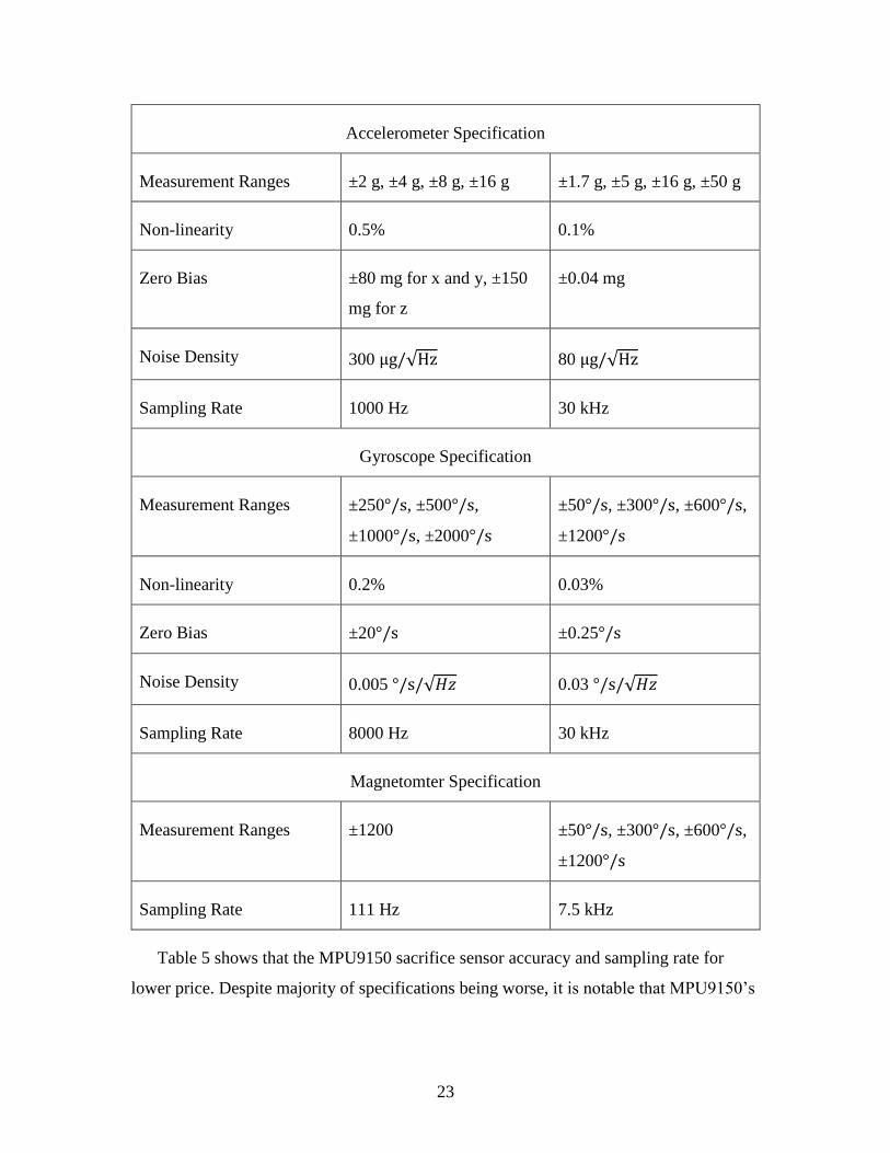
Table 5: Comparison of sensor specifications between MPU9150 and 3DM-GX3

Item MPU9150 3DM-GX3

23

Accelerometer Specification

Measurement Ranges ±2 g, ±4 g, ±8 g, ±16 g ±1.7 g, ±5 g, ±16 g, ±50 g

Non-linearity 0.5% 0.1%

Zero Bias ±80 mg for x and y, ±150

mg for z

±0.04 mg

Noise Density 300 μg/√Hz 80 μg/√Hz

Sampling Rate 1000 Hz 30 kHz

Gyroscope Specification

Measurement Ranges ±250°/s, ±500°/s,

±1000°/s, ±2000°/s

±50°/s, ±300°/s, ±600°/s,

±1200°/s

Non-linearity 0.2% 0.03%

Zero Bias ±20°/s ±0.25°/s

Noise Density 0.005 °/s/√𝐻𝑧 0.03 °/s/√𝐻𝑧

Sampling Rate 8000 Hz 30 kHz

Magnetomter Specification

Measurement Ranges ±1200 ±50°/s, ±300°/s, ±600°/s,

±1200°/s

Sampling Rate 111 Hz 7.5 kHz

Table 5 shows that the MPU9150 sacrifice sensor accuracy and sampling rate for

lower price. Despite majority of specifications being worse, it is notable that MPU9150’s

24

gyroscope has lower noise density than 3DM-GX3. The following are a few other

comparisons.

MPU9150 uses ADCs to digitalize the analog outputs: three 16-bit ADCs for

gyroscope readings, three 16-bit ADCs for accelerometer readings, three 13-

bit ADCs for magnetometer readings. 3DM-GX3 also uses 16-bit ADC.

MPU9150 has a very robust 10,000 g shock tolerance, while 3DM-GX3 only

has 500g shock tolerance

MPU9150 could also help save power for the sensor node as well, because of its 1024

B FIFO buffer which allows data to be read by the system processor in bursts. Then the

system processor could enter sleep mode while the MPU9150 continues to collect data to

fill the buffer.

3.2.3 Bluetooth Smart module: BLE113

The Bluegiga BLE113 module is based on Texas Instruments’ CC2541 chip, and has

all the features required for a Bluetooth Smart application. The following components are

integrated in the module: a Bluetooth Smart radio, software stack, and GAP, GATT

support. BLE113 is compliant to wireless certifications of all major countries in the

world. The radio has transmission power from 0 dB to -23 dB, and receiver sensitivity of

-93 dB. The module consumes ultra-low current, as low as 500 nA while in sleeping

mode, and can wake up in less than a couple of milliseconds. During transmission, the

module’s current consumption is between 14.3 mA and 27 mA. The module uses UART

as the primary interface with an external processor, and it also has peripheral interfaces of

SPI, I2C, PWM, and GPIO. The module even has a 12-bit ADC. These peripheral

interfaces and the ADC are for the microprocessor incorporated inside the module.

BLE113 contains a Texas Instruments’ 8051 microprocessor core which could be

used for standalone operations. It has 8 KB SRAM, and 128/256 KB Flash memory.

However, this microprocessor core could only be programmed with BGScript, a special

script for Bluegiga modules, which is unable to handle complicate programs and

configurations. Furthermore, there is no debugger for this microprocessor, making the

25

development process much less convenient. These problems significantly limit the 8051

core’s already relatively poor performance. Hence this integrated microprocessor is not

utilized for this project.

3.3 Microcontroller software Design

The sensor node contains a powerful Cortex-M4 microprocessor that supports

software with many floating point manipulations. The software is primarily developed to

capture sensor measurements and send them to the BLE module for transmission.

Additional features such as basic data processing and sensor fusion could be added to

reduce the bandwidth needed for transmission without compromising data accuracy and

timeliness.

In this section, the basic operations in the software that are needed for the sensor node

to work is presented.

3.3.1 Initialization and configuration

The microcontroller software program is developed in Texas Instruments’ Code

Composer Studio v5.2 environment, with library for TM4C123GH microprocessor.

At start, the software is programmed to initialize the pointers to store the sensor

readings and sensor fusion results. There are at most 16 float data coming out from the

MPU9150 sensor for each iteration. Among these 16 floats, 3 floats are for 3-axis

accelerometer data, 3 floats are for 3-axis gyroscope data, 3 floats are for 3-axis

magnetometer data, 3 floats are for the Euler angle outputs, and the last 4 floats are for

the Quaternion results. This arrangement allows all sensor data and sensor fusion results

to be collected and calculated.

Next the microcontroller system properties are configured and the I/O ports with

MPU9150 and BLE113 are initialized, as shown in Figure 5. The system clock is set to

40 MHz from PLL with 16 MHz crystal reference. GPIO A is set up for UART0, which

is used to print messages to PC via ICDI for debugging. Port A0 is configured to be the

receiving pin and port A1 is configured to be the transmitting pin. The 16 MHz oscillator

26

is used as the clock source for this UART channel, and the baud rate is set to be 115,200.

UART4 channel for communication with the BLE113 module is set up in similar way,

with port C4 as the receiving pin and port C5 as the transmitting pin. UART4 does not

use flow control, but instead transmits data in packet mode. This is to simplify the

communication with BLE113 module. The baud rate of UART4 is also 115,200, same as

UART0. To trigger the corresponding method whenever a new event or response comes

from the BLE113 module, the UART4 is set to interrupt the main program once a receive

event or a receive timeout event happens.

27

void ConfigureUART(void) { // // Enable UART0 // ROM_SysCtlPeripheralEnable(SYSCTL_PERIPH_GPIOA); ROM_SysCtlPeripheralEnable(SYSCTL_PERIPH_UART0); // // Configure GPIO Pins for UART mode. // ROM_GPIOPinConfigure(GPIO_PA0_U0RX); ROM_GPIOPinConfigure(GPIO_PA1_U0TX); ROM_GPIOPinTypeUART(GPIO_PORTA_BASE, GPIO_PIN_0 | GPIO_PIN_1); // // Use the internal 16MHz oscillator as the UART clock source. // UARTClockSourceSet(UART0_BASE, UART_CLOCK_PIOSC); // // Initialize the UART for console I/O. // UARTStdioConfig(0, 115200, 16000000); // Configure URAT4 ROM_SysCtlPeripheralEnable(SYSCTL_PERIPH_GPIOC); ROM_SysCtlPeripheralEnable(SYSCTL_PERIPH_UART4); ROM_GPIOPinConfigure(GPIO_PC4_U4RX); ROM_GPIOPinConfigure(GPIO_PC5_U4TX); ROM_GPIOPinTypeUART(GPIO_PORTC_BASE, GPIO_PIN_4 | GPIO_PIN_5); // // Configure the UART for 115,200, 8-N-1 operation. // UARTConfigSetExpClk(UART4_BASE, ROM_SysCtlClockGet(), 115200, (UART_CONFIG_WLEN_8 | UART_CONFIG_STOP_ONE | UART_CONFIG_PAR_NONE)); UARTFlowControlSet(UART4_BASE, UART_FLOWCONTROL_NONE); // // Enable the UART interrupt. // UARTIntDisable(UART4_BASE, 0xFFFFFFFF); UARTIntEnable(UART4_BASE, UART_INT_RX | UART_INT_RT); IntEnable(INT_UART4); }

Figure 5: Code snippet for configuring UART channels

28

After the UART4 channel is set up, a few library functions are called to initialize

BLE113 module for connection with a remote BLE device. A few global variables,

g_bleUserFlag, g_bleFlag, and g_bleDisconnectFlag, form the state machine for

BLE113 module. Before initialization, all flags are set to 0 (false). The initialization starts

by calling ble_cmd_system_reset method, which sends command to reset the BLE113

module. Once the reset is complete, the response comes back, generating a system boot

event. Then the program continues to set GAP mode and bondable mode in sequence, as

shown in Figure 6. If the response comes back indicating the commands fail, then the

program resets the BLE113 module again and repeats the process. When both GAP mode

and bondable mode are set successfully, the BLE113 becomes ready for connection with

remote BLE device. At this time, g_bleFlag is set to 1 (true) so the program knows the

BLE113 module is ready. The details about sending commands and interpreting

responses are described in sub-section 3.3.3 of this chapter.

void ble_evt_system_boot(const struct ble_msg_system_boot_evt_t * msg) { UARTprintf("System booted!\n"); g_bleUserFlag = 0; ble_cmd_gap_set_mode(gap_general_discoverable, gap_undirected_connectable); } void ble_rsp_gap_set_mode(const struct ble_msg_gap_set_mode_rsp_t * msg) { if (msg->result == 0) { UARTprintf("GAP mode set successful!\n"); ble_cmd_sm_set_bondable_mode(1); } else { UARTprintf("GAP mode set fail: %u\n", msg->result); ConfigureBLE(); } } void ble_rsp_sm_set_bondable_mode(const void* nul) { UARTprintf("Bond mode set.\n"); g_bleFlag = 1; }

Figure 6: Code Snippet for preparing the BLE113 module for connection

29

// Initialize the MPU9150 Driver. MPU9150Init(&g_sMPU9150Inst, &g_sI2CInst, MPU9150_I2C_ADDRESS, MPU9150AppCallback, &g_sMPU9150Inst); // Wait for transaction to complete MPU9150AppI2CWait(__FILE__, __LINE__); // Configure the sampling rate. g_sMPU9150Inst.pui8Data[0] = 4; MPU9150Write(&g_sMPU9150Inst, MPU9150_O_SMPLRT_DIV, g_sMPU9150Inst.pui8Data, 1, MPU9150AppCallback, &g_sMPU9150Inst); MPU9150AppI2CWait(__FILE__, __LINE__); // Write application specificed sensor configuration such as filter // settings and sensor range settings. g_sMPU9150Inst.pui8Data[0] = MPU9150_CONFIG_DLPF_CFG_94_98; g_sMPU9150Inst.pui8Data[1] = MPU9150_GYRO_CONFIG_FS_SEL_250; g_sMPU9150Inst.pui8Data[2] = (MPU9150_ACCEL_CONFIG_ACCEL_HPF_5HZ | MPU9150_ACCEL_CONFIG_AFS_SEL_2G); MPU9150Write(&g_sMPU9150Inst, MPU9150_O_CONFIG, g_sMPU9150Inst.pui8Data, 3,MPU9150AppCallback, &g_sMPU9150Inst); MPU9150AppI2CWait(__FILE__, __LINE__); // Configure the data ready interrupt pin output of the MPU9150. g_sMPU9150Inst.pui8Data[0] = MPU9150_INT_PIN_CFG_INT_LEVEL | MPU9150_INT_PIN_CFG_INT_RD_CLEAR | MPU9150_INT_PIN_CFG_LATCH_INT_EN; g_sMPU9150Inst.pui8Data[1] = MPU9150_INT_ENABLE_DATA_RDY_EN; MPU9150Write(&g_sMPU9150Inst, MPU9150_O_INT_PIN_CFG, g_sMPU9150Inst.pui8Data, 2, MPU9150AppCallback, &g_sMPU9150Inst); MPU9150AppI2CWait(__FILE__, __LINE__); // Initialize the DCM system. 50 hz sample rate. // accel weight = .2, gyro weight = .8, mag weight = .2 CompDCMInit(&g_sCompDCMInst, 1.0f / 50.0f, 0.2f, 0.6f, 0.2f);

Figure 7: Code Snippet for the MPU9150 initialization sequence

30

Since the UART channels and BLE113 modules are initialized and ready, next step is

to implement the initializations of I2C channel and MPU9150 sensor. The

microcontroller communicates with MPU9150 through I2C3 channel residing on GPIOD

port. The SCL pin is set to be D0 and the SDA pin is set to be D1. GPIOE port E2 pin is

used for interrupts from MPU9150, with the interrupt mask set to falling edge only. A

system function ROM_IntMasterEnable is called to enable all interrupts to the

microprocessor. The I2C3 peripheral is then initialized, allowing commands to be sent

from the microcontroller to MPU9150, as illustrates in Figure 7. At first, the initialization

command is sent to MPU9150, with pointers of driver instances and callback. For each

command, the program needs to wait for the response before sending a new command. If

the wait times out, the program reports the error by setting the LED to blink red light with

10 Hz frequency. The second command is to set the sampling rate. The parameter integer

plus one is used to divide 1 KHz. For example, the result sampling rate would be 200 Hz

if the parameter is 4. The third command sets specific sensor configurations such as range

selections. It also sets the filters for both accelerometer and gyroscope. The forth

command configures the data ready pin output for MPU9150 so it can successfully

generate an interrupt to the microprocessor. The last command initializes the Direction

Cosine Matrix (DCM) calculation, allowing the program to set sampling frequency and

specify weights for accelerometer, gyroscope, and magnetometer. The DCM library is

included in the example code provided by Texas Instruments as part of the software stack

for the TM4C microcontroller. The algorithm in DCM library is basically a

complementary filter that can calculate Euler angles and Quaternions from the outputs of

a 9-axis sensor. There's a global flag indicating whether the DCM algorithm is running.

In the last section of the initialization, the tri-color LED is configured to blink at 1

Hz, with half the intensity and white color. Then the EEPROM is initialized so that the

program can read the configurations saved in EEPROM. The EEPROM could also save

the error estimations calculated by the calibration process for the sensor node.

With the initializations done, the program enters an infinite loop, continuously

reading data from MPU9150 and waiting for connection from the remote data processing

device.

31

3.3.2 Data and control flow

Figure 8 shows communication protocol between the TM4C123GH microcontroller

and the BLE113 module, MPU9150 sensor. After initialization, the system is designed to

continuously read the measurements from the sensor and transmit the data to remote data

processing device if it’s connected.

Every iteration of the loop, the software is programmed to loop check a flag for the

sensor data to arrive. Whenever a new measurement is ready to read, the interrupt pin E2

is forced to low voltage by MPU9150 to alert the microcontroller. Detecting the falling

edge, the interrupt service routine is invoked and the flag is set to true to break the loop.

Then the system sends a read request to accelerometer, gyroscope, magnetometer each,

and the measurements are transmitted to the microcontroller over I2C. This mechanism is

there to ensure the data are read at desired frequency.

At this point, the program already has the raw data from the 9-axis sensor. The

microcontroller could do some basic processing, such as removing biases in sensor

measurements, before sending the data. It is also possible to apply very complicate filters

to the results for better accuracy. In addition the microcontroller can calculate Euler angle

and Quaternion data with the DCM library. The DCM algorithm passes the data from

accelerometer, gyroscope, and magnetometer into a complimentary filter. The result is a

rotation matrix, and further calculation could yield Euler angle and Quaternion results.

The main purpose of doing some data processing at sensor node is to reduce the amount

of data being transmitted to the remote BLE device. If applications only require Euler

angles or Quaternions, there is no need to transmit raw sensor readings.

TM4C123GH

Microcontroller

MPU9150

Motion Sensor

BLE113 Module

I2C UART

Figure 8: The figure above shows the data flow from sensor to the Bluetooth

module.

32

For transmission of the data, if the Bluetooth Smart module has already indicated that

the remote data processing device is connected, the global flag g_bleUserFlag is set to 1

(true). Then the data can be transmitted to BLE113 via UART and written to the

corresponding attribute in the GATT table. For each type of sensor or DCM results, the

program needs to send one attribute write command. If the system requires transmitting

more than one type of results, then in the same cycle the next transmission must wait

until the response to previous transmission is received. Otherwise, the UART channel

between the microcontroller and the BLE113 module might be jammed with excess data,

causing problems in future transmissions. The reason is, when there are too much data in

transmission, the BLE113 module might miss one byte or more, causing the module to

wait on the missing bytes even after the transmission is finished.

If the connection is broken due to operations on the remote device or going out of

range, the microcontroller is notified of the event by the BLE module, setting the global

flag g_bleUserFlag to 0 and g_bleDisconnectFlag to 1. By this way in next iteration the

program will detect the flags, stop attempting to transmit the data and call the method to

configure the BLE113 module for reconnection. Therefore, even if a disconnection

happens (most likely due to sensor node moving out of range), a new connection can be

established as soon as the pair of devices are ready and in range.

3.3.3 Implementation of BGLib

The BGLib is the C library for the Bluegiga BLE113 to work with external

microprocessor. It contains various commands, events, responses, and their

corresponding UART channel messages. When sending a command, the library functions

translate the command to a message and send it over UART; when receiving an event or

response, the library functions interpret the message received and trigger the correct

method to handle the received event or response. The implementation of BGLib requires

writing two methods: one for input from and one for output to the UART channel.

The input method is designed to receive data from the UART channel, interpret the

header of the message, and call the handler from BGLib to process the message. Since

the message coming from BLE113 does not have fixed length, the program needs to

33

figure out how long the message is in total. Whenever an interrupt happens for UART4,

the input method is called. The first 4 bytes of the message are read and saved into a

header struct. The header struct determines the type of the message and how many bytes

of payload the message has. The BGLib functions are called to transform the header

struct to a constant struct type called ble_msg, which points to the corresponding handler

function according to the type of the message. Then the program could read an exact

number of bytes as the payload, and save them in a separate data array. Finally the

handler function is invoked with the payload data array as a parameter. This handler

function is declared in BGLib and implemented in the main program. Since the message

is from BLE113 to the microcontroller, it would be either an event or a response. If the

message is an event, then the program could do something in response to it; if the

message is a response for a previously sent command, then the program could find out

whether the command was executed successfully or not. Figure 9 shows the

implementation of some of the handling methods in the main program. The events such

as boot-up, connection, and disconnection would trigger the program to initialize

BLE113, set the flag to allow data transmission to it, and prepare it for reconnection

respectively. The response ble_rsp_gap_set_mode leads to sending next command in

initialization sequence, ble_cmd_sm_set_bondable_mode to BLE113. Another response

ble_rsp_attributes_write leads to setting the flag indicating new write command could be

sent to BLE113 now.

34

void ble_evt_system_boot(const struct ble_msg_system_boot_evt_t * msg) {

UARTprintf("System booted!\n");

g_bleUserFlag = 0;

ble_cmd_gap_set_mode(gap_general_discoverable,

gap_undirected_connectable);

}

void ble_rsp_gap_set_mode(const struct ble_msg_gap_set_mode_rsp_t * msg)

{

if (msg->result == 0) {

UARTprintf("GAP mode set successful!\n");

ble_cmd_sm_set_bondable_mode(1);

} else {

UARTprintf("GAP mode set fail: %u\n", msg->result);

ConfigureBLE();

}

}

void ble_rsp_sm_set_bondable_mode(const void* nul) {

UARTprintf("Bond mode set.\n");

g_bleFlag = 1;

}

void ble_evt_connection_status(

const struct ble_msg_connection_status_evt_t *msg) {

UARTprintf("Got here\n");

// New connection

if (msg->flags & connection_connected) {

g_bleUserFlag = 1;

UARTprintf("Connected\n");

}

}

void ble_evt_connection_disconnected(

const struct ble_msg_connection_disconnected_evt_t *msg) {

UARTprintf("Disconnected: %u\n", msg->reason);

g_bleUserFlag = 0;

g_bleDisconnectFlag = 1;

}

void ble_rsp_attributes_write(const struct ble_msg_attributes_write_rsp_t

*msg) {

if (msg->result == 0) {

//UARTprintf("Attribute write successful\n");

} else {

UARTprintf("Attribute write failed: %x\n", msg->result);

}

g_bleFlag = 1;

}

Figure 9: Code snippet for some of the handling methods of BLE events and

responses

35

For the output method, its responsibility is to output messages to the UART channel

in the correct format. By design, the output method is not directly called by the main

program. For every specific command, a BGLib method is defined to arrange the

message for the command, and sends the message to the abstract method bglib_output.

When the main program wants to send a command to BLE113, the corresponding BGlib

method is called. To connect the BGLib function with the user-defined output method,

the pointer of bglib_output is assigned to the pointer of ouput during initialization. This

way when the BGLib calls the bglib_output function, it is actually the output function

that gets called. As stated in sub-section 3.3.1, the UART communication from the

microcontroller to BLE113 is in packet mode. This means that for output, before sending

the actual message, the total length of the message needs to be sent first. Then, the actual

message can be written to the UART4 channel in two parts. The first part is the 4-byte

long header, which contains the message type, the number of bytes of payload, and other

configurations. The second part is the payload, such as the collected sensor data ready to

send to the remote data processing device. The nature of this type of communication

requires time separation between transmissions. Normally it's only safe to transmit a new

message after the response to the previous message is received.

To finish the implementation, all the relevant events, responses are handled by the

system. Table 6 shows the necessary events, responses, commands needed for the

program to achieve basic functionalities.

Table 6: Commands, Events, and Responses for sensor node to have basic functions

Name Type Function

ble_cmd_system_reset Command Reset the BLE113 module

ble_cmd_gap_set_mode Command Configure the GAP mode

ble_cmd_sm_set_bondable_mode Command Set BLE113 to bondable mode

ble_cmd_system_hello Command Expect BLE113 to respond with

ble_rsp_system_hello

36

ble_cmd_system_get_info Command Expect BLE113 to respond with

ble_rsp_system_get_info

ble_cmd_attributes_write Command Send data to the corresponding

GATT attributes

ble_rsp_gap_set_mode Response Indicate whether GAP mode is set

successfully

ble_rsp_sm_set_bondable_mode Response Indicate BLE113 has received

ble_cmd_sm_set_bondable_mode

ble_rsp_system_hello Response Indicate BLE113 has received

ble_cmd_system_hello

ble_rsp_system_get_info Response Contain information for build

number, protocol version, and

hardware

ble_rsp_attributes_write Response Indicate whether the write is

successful

ble_evt_system_boot Event Indicate that BLE113 has booted

ble_evt_connection_status Event Indicate connection established,

contain the current connection status

ble_event_connection_disconnected Event Indicate connection disconnected,

contain the reason for disconnection

3.3.4 Simple calibration

The MPU9150 sensors sometimes have significant errors in raw measurements,

therefore before actually deploying the system, all the sensor nodes should be

individually calibrated to estimate the most common errors: zero biases and scale factors.

37

However the basic calibration procedures of the embedded accelerometer, gyroscope, and

magnetometer are vastly different. For the accelerometer, the approach is to measure the

output of one axis with actual gravity equal to –g, 0, and g. It is then possible to use these

measurements to calculate the zero bias and scale factor for each axis. For the gyroscope,

the zero biases are basically the stationary readings, while the scale factors require

integrating the measurements as the sensor rotates a certain angle around each axis.

Calibrating the magnetometer, on the other hand, is much harder. Rigorous magnetometer

calibration involves taking thousands of measurements of different orientations in a 3D

space.

A simple calibration procedure is developed for the project. It is included in the

microcontroller software of every sensor node. The aim is to measure the accelerometer

zero biases and scale factor, plus the gyroscope zero biases. The magnetometer

calibration is not possible with the sensor node alone, therefore it is omitted. It is also

difficult to perform accurate measurements for gyroscope scale factors since it requires

integrating the noisy readings. The calibration mode is programmed to start as the

calibration button (one of the two programmable buttons) on the sensor node board is

pressed. The calibration process has 3 stages, each with different placement of the sensor

node. In the first stage, the z axis points downward along the direction of the gravity. The

second and third stage are for the y and x axes respectively. The LED changes color to

indicate different stages, and the calibration button needs to be pressed to proceed to next

stage. Readings from the accelerometer and the gyroscope are averaged for every stage to

get measurement values of the accelerometer corresponding to 0 (𝑎0) and gravity (𝑎𝑔)

along each axis, and zero biases for the gyroscope. While zero biases of the

accelerometer are just 𝑎0, scale factors for the accelerometer is calculated using the

following equation.

scale factor =(𝑎𝑔 − 𝑎0)

𝑔

Once complete, the microcontroller saves the correction values in EEPROM for real-

time use with the raw sensor data to produce more accurate estimates.

38

However, this simple calibration method could introduce errors because the sensor

axes might not be perfectly aligned with the gravity during calibration. Hence the

calibration process needs to be carefully executed to minimize the errors.

3.4 Bluetooth Smart module configuration

The BLE113 module is programmed separately from the rest of the system by

attaching a Texas Instruments’ CC debugger to the 2 × 5 pin heads on the sensor node

board, and connecting the CC debugger to PC. Bluegiga provides tools to compile and

upload the configuration files to BLE113. There are 3 configuration files: cdc.xml,

gatt.xml, and hardware.xml. Several examples of working systems are provided as well.

Based on an example for interacting with external microprocessor, only settings in

gatt.xml and hardware.xml need to be modified to adapt to our system, and cdc.xml can

be left untouched.

3.4.1 Configurations in hardware.xml

Figure 10 shows the content of the modified hardware.xml for the sensor node.

The most important part of this document is the UART configuration on the third

line. This line specifies which UART channel to communicate with the external

microprocessor, the baud rate of the channel, the flow control status, and whether the

transmission is in packet mode or not. This line also tells the BLE113 module to execute

the BGAPI commands by making the endpoint "api". BGAPI can interpret incoming

Figure 10: Content of hardware.xml for the sensor node

39

UART messages and execute accordingly. BGAPI can also output message to UART

channel to report an event or respond to a command. These settings need to be matched

with the implementation of the microcontroller software.

Other lines are mostly unchanged from the original example provided by Bluegiga.

Note that sleep is disabled for debugging purpose. It can be enabled, but then before

every transmission, the microprocessor needs to send a signal to the wakeup pin as

specified. In this case if sleep is enabled, the microprocessor needs to send a rising edge

signal to port 0 pin 0 of the BLE113 module to wake it up.

3.4.2 Configurations in gatt.xml

The gatt.xml determines configurations for the Generic Attributes Profile (GATT).

The GATT stores data, also called attributes, in characteristics. A characteristic contains:

Characteristic Declaration - configurations that describe the properties of the

Characteristic Value, its Universally Unique Identifier (UUID) and handle for

access

Characteristic Value - a value with known format

Characteristic Descriptor - additional text that provides information about the

characteristic

The property of characteristic value regulates how the data could be transmitted.

There are mainly 5 types of properties: const, read, write, notify, and indicate.

Const means the characteristic value is constant.

Read is for the remote device to actively send a read command to the BLE113

module, and gets the current value in response from the module.

Write is for the remote device to modify the value in this characteristic.

40

Notify, when enabled by remote device, lets the BLE113 module automatically

send the data in characteristic to the remote device, whenever new values come

in from the microprocessor.

Indicate is like notify, but the remote device need to send a confirmation each

time the BLE113 module sends a value.

Other properties include authenticated read and write, adding an authentication

requirement for the read and write operations.

Several characteristics could be grouped together as a service. Each service and

characteristic needs to have a unique randomly-generated UUID for reference.

In our sensor node system, the GATT has a simple structure. The first service

provides information about the BLE113 module, such as device name and reconnection

address. The second service contains information of the hardware, including the

manufacturer, the model name, and the serial number. The third service is for battery

information. The next 3 services correspond to each individual sensor: accelerometer,

gyroscope, and magnetometer. Each service contains one characteristic that stores 12

bytes long data, enough to transmit 3 float results, one for each axis. It is arranged in this

way so that it only takes one write to transmit all the data for one type of sensor results to

the BLE113 module, reducing the traffic on the UART channel between the

microprocessor and the BLE113 module. Then there is the service for the Euler Angle

output from DCM library. Similarly, the Euler angle service has a characteristic of 12-

byte length, enough to hold all results.

41

Chapter 4: Application Example – Personal Navigation System

An example application, MotionTracker, is designed to demonstrate the advantages of

the inertial sensor network proposed in this thesis. The core concept is to use the Euler

angles measured by the sensor nodes placed on a person’s legs to determine the angles of

legs relative to the ground, and find out the step length using trigonometry. This is similar

to human motion tracking. E. R. Bachman et al. designed an efficient motion tracking

system for humans and robots, using Quaternions calculated by a complementary filter

[18]. The system is able to accurately track the orientation of a rigid body with a large

sensor pack that measures 10.7 cm, 5 cm, and 3.7 cm for length, width, and height. It is

not practical to wear such a large sensor on the human body. Another research from

Tsinghua University uses a Kalman filter to compute the orientation of human body

segments [19]. In the experiment they let a subject move arm horizontally and vertically,

with sensors placed on the subject’s shoulder, upper arm, and lower arm. They were able

to achieve an error of less than 1 cm for all axes when results are combined from 3

sensors. However, the data output of the system has a 0.9 second delay. Compared to

these examples, the MotionTracker model is simplified to just account for the walking

associated lower body motion. With this constraint, Euler angles can be used without

worrying about the singularities. Unlike Quaternions, the Euler angles can be directly

used for calculation to find step length. The MotionTracker system is designed to report

real-time Euler angle data of the legs with minimum delay through Bluetooth Smart to

users’ smartphones.

As shown in Figure 11, MotionTracker is composed of a remote data processing

device and at least 4 sensor nodes which measure the angles of the limbs relative to the

gravity. These 4 sensor nodes are tightly attached to the legs of the user. The legs are

divided into 4 parts, the upper left leg (part 1), lower left leg (part 2), upper right leg (part

3), and lower right leg (part 4); each part has one sensor node on the front, placing around

the knees, with its y direction facing upward along the leg, its x direction toward the right

side, and its z direction going into the leg. Each sensor node computes the angle of the

part of leg it attached to and transmits the results to a smartphone, via Bluetooth Smart.

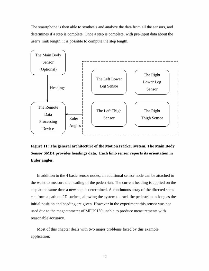
42

The smartphone is then able to synthesis and analyze the data from all the sensors, and

determines if a step is complete. Once a step is complete, with pre-input data about the

user’s limb length, it is possible to compute the step length.

In addition to the 4 basic sensor nodes, an additional sensor node can be attached to

the waist to measure the heading of the pedestrian. The current heading is applied on the

step at the same time a new step is determined. A continuous array of the directed steps

can form a path on 2D surface, allowing the system to track the pedestrian as long as the

initial position and heading are given. However in the experiment this sensor was not

used due to the magnetometer of MPU9150 unable to produce measurements with

reasonable accuracy.

Most of this chapter deals with two major problems faced by this example

application:

Figure 11: The general architecture of the MotionTracker system. The Main Body

Sensor SMB1 provides headings data. Each limb sensor reports its orientation in

Euler angles.

The Main Body

Sensor

(Optional)

The Left Lower

Leg Sensor

The Right

Lower Leg

Sensor

The Left Thigh

Sensor

The Right

Thigh Sensor

The Remote

Data

Processing

Device

Headings

Position

Euler

Angles

43

How to determine the current step length?

How to differentiate between steps?

After that, more discussions about the software implementation of remote data

processing device are followed.

4.1 How to determine the current step length

To measure the step length, the length of legs must be known. As Figure 12 shows,

the lengths of the upper legs are denoted as L1 (left), L3 (right), and the lengths of the

lower legs are denoted as L2, L4. These lengths are measured from joint to joint for best

accuracy; for example, L2, L4 are measured from ankle to knee.

The Euler angles are most commonly used to describe the orientation of an object. In

the context of this example application, the Euler angles describe the orientation of the

sensor nodes, and the limb they attach to. By definition, the roll of the Euler angles

represents the rotation of sensor node board around X’-axis from the ground. The X’-axis

is the result of rotating the X-axis of Earth reference frame by the yaw angle (heading).

This angle is most useful in the calculation of step length, and it is denoted as E1x for

upper left leg. The pitch of the Euler angles represents the relative angle around z-axis of

L2

L1

L3

L4

Figure 12: A pedestrian stepping with his right leg

44

the sensor between the sensor node board and the ground. It is as denoted E1y for the

same limb. The yaw of the Euler angles represents the heading of the sensor node on the

ground plane (around Z-axis of Earth frame). It is denoted as E1z. The Euler angles for

other parts of the legs are denoted similarly. Based on these results, the system could

calculate the horizontal displacements of the two feet (DL, DR) along main direction

(front and back) relative to a virtual origin. Figure 13 below denotes Euler angles and

horizontal displacements of the two feet along the primary direction. Using trigonometry,

the displacements can be calculated as follows:

𝐷𝐿 = cos 𝐸1𝑥 × 𝐿1 + cos 𝐸2𝑥 × 𝐿2

𝐷𝑅 = cos 𝐸3𝑥 × 𝐿3 + cos 𝐸4𝑥 × 𝐿4

However this calculation does not include possible sideway inclinations of the legs.

The legs might not be confined to the plane defined by the gravity and the walking

direction, as shown in Figure 13. More often than not, the legs stretch sideway while

DL DR

E3x

E1x

E2x

E4x

Figure 13: Denotations of Euler angles and relative displacements along primary

direction, viewed from the side of pedestrian

45

walking or standing, as depicted in Figure 14. The step length along the primary walking

direction is thus needed to be computed from the actual leg lengths’ projections. The

actions of side-stepping and going on stairs are not considered in MotionTracker, so there

are no calculations for displacements of the two feet along any directions other than front

and back.

Hence the new formulas that consider this effect is presented below:

𝐷𝐿 = cos 𝐸1𝑦 × cos 𝐸1𝑥 × 𝐿1 + cos 𝐸2𝑦 × cos 𝐸2𝑥 × 𝐿2

𝐷𝑅 = cos 𝐸3𝑦 × cos 𝐸3𝑥 × 𝐿3 + cos 𝐸4𝑦 × cos 𝐸4𝑥 × 𝐿4

By comparing the two values, it is possible to determine which foot is at front, and

the difference with the other foot is the step length at that moment. With the provided

information, it may be possible to find out whether the pedestrian is walking forward or

backward; but this would involve analyzing all the angles carefully through a step and

knowledge in human walking pattern, which is beyond the scope of this thesis. For

E2y E

1y E

3y E

4y

Figure 14: Denotation of Euler angles, viewed from the back of pedestrian

46

MotionTracker, the assumption of a pedestrian always walks forward is made. Therefore

only the step length S is needed to calculate the walking path of the pedestrian. For the

instance in Figure 13 the step length can then be calculated as follows:

S = |𝐷𝑅 − 𝐷𝐿|

However this step length could not be directly used for accumulation to get the total

distance travelled by a pedestrian. In fact, the sensor data can come at any time during a

step and it is not guaranteed to be the moment when both feet are on the ground. This

problem could be resolved by using a 5th sensor as pedometer to count the step.

Alternatively, another method is used to determine when a step is finished.

4.2 How to differentiate between steps

It can be inferred that for normal walking biomechanics, the actual step length is

closest to the maximum step length recorded in a step’s time. To find the exact moment a

step is finished, is equivalent to find the moment DR becomes larger than DL or vice

versa. However, because of the presence of noises, this might happen multiple times

during a step, especially when the data rate is high. To avoid noises causing the system to

miscount the steps, a step threshold, denoted as ES, needs to be applied. ES is determined

by the error in angles and limb length. Only when the step length S (the absolute

difference between DR and DL) is greater than the threshold ES, the system can conclude

that the pedestrian is really making a step. To determine the boundary between multiple

steps made by the pedestrian, it is also vitally important to detect which foot is at front.

Consider the normal walking pattern, both feet alternate to be in the front. Hence in our

system, a new step only happens if the other foot comes to the front, while the step length

S is greater than the threshold Es.

The standing situation also needs to be considered. When the pedestrian is standing

still, the two feet should be close to each other and the step length S should be constantly

around 0. Hence the program understands that the pedestrian is standing when the step

length S is consistently less than the threshold Es for an extended period of time. In this

case there is not a single feet that is at the front. When the pedestrian starts to walk, the

47

step length S becomes greater than the threshold Es. At this moment the program needs to

find out the feet at front for the first step, and set the state to walking state. When the

pedestrian stops walking to stand still, the program needs to check the step length for a

number of iterations based on the data rate. This is done by defining a count KS, which is

incremented for every iteration with the step length S less than the threshold Es. If KS

becomes equal or greater than a constant number C, the current step is finished and the

state is set to standing state. The constant C should be dependent on the data rate,

allowing the program to detect the standing mode in the timeframe of 1 or 2 seconds.

Table 7 shows the complete state machine for the MotionTracker system.

Table 7: The state machine for MotionTracker

Current State Condition Next State Effect

Standing State S < Es Standing State

Standing State S > Es and DL > DR Walking State,

Left

Start a new step

Standing State S > Es and DR > DL Walking State,

Right

Start a new step

Walking State,

Left

S > Es and DL > DR Walking State,

Left

reset KS

Walking State,

Left

S > Es and DR > DL Walking State,

Right

Finish current step, start

a new step, reset KS

Walking State,

Left

S < Es and KS < C Walking State,

Left

Increment KS

Walking State,

Left

S < Es and KS > C Standing State Finish current step,

reset KS

48

Walking State,

Right

S > Es and DL > DR Walking State,

Left

Finish current step, start

a new step, reset KS

Walking State,

Right

S > Es and DR > DL Walking State,

Right

reset KS

Walking State,

Right

S < Es and KS < C Walking State,

Right

Increment KS

Walking State,

Right

S < Es and KS > C Standing State Finish current step,

reset KS

The rare situation in which the pedestrian stops in the middle of a step with two feet

separated is not considered here. This situation is somewhat covered in the current state

machine. Since the step length does not close, the step does not finish, and the current

recorded maximum step length will be kept for the whole duration of the stop. As the

pedestrian starts walking again the final step length could be determined as the step

finishes.

The step length of a step is only recorded when the step is finished. At this moment,

the current maximum step length over the entire duration of the step become the recorded

step length of this step, and is thus added to the total distance walked by the pedestrian.

4.3 Android app design

In the MotionTracker system, the remote data processing device is developed on

Android platform. The MotionTracker Android app handles the Bluetooth Smart

communications similar to the example app provided by Texas Instrument for its

SensorTag [20]. The service that controls connections from the example app is retrofitted

to allow multiple sensor nodes connecting to one Android device at the same time. When

connections are established, the MotionTracker app receives continuous updates of Euler

angles, calculates the step lengths and total distances walked, and displays the results to

the user.

49

The app starts with the scanning interface where all broadcasting sensor nodes of the

system are listed and available for connection, while other BLE devices are filtered. The

user could touch the listed sensor to establish connection. Once all the connections are

established, a button can be pressed to start the system. The app enters the interface that

display Euler angles sent from all the sensor nodes. At the same time, the app commands

the sensor nodes to send notifications when new data are available. A broadcast receiver

handles all interrupts from the BLE module on the smartphone and invokes actions when

new data arrive from the sensor nodes. These actions include updating the interface with

the newest values and analysis results.

Before actually calculating the step length, the app needs to pair the sensor nodes

with the locations they are attached to, and load the lengths of limb. These parings and

lengths of limb have to be given by a user. The user could change these settings in the

preferences.

After these preparations the app is ready to start recording and calculating the how

pedestrian walks. At the start, the system is initialized into standing mode. Then, as

described in sections 4.1 and 4.2, the app enters a state machine to count the steps,

determine the step length, and eventually calculate the total distance walked by a user.

These results are reported to the user interface of the app on the run.

The source code and the instructions to load the program to an Android device can

be found in Appendix C.

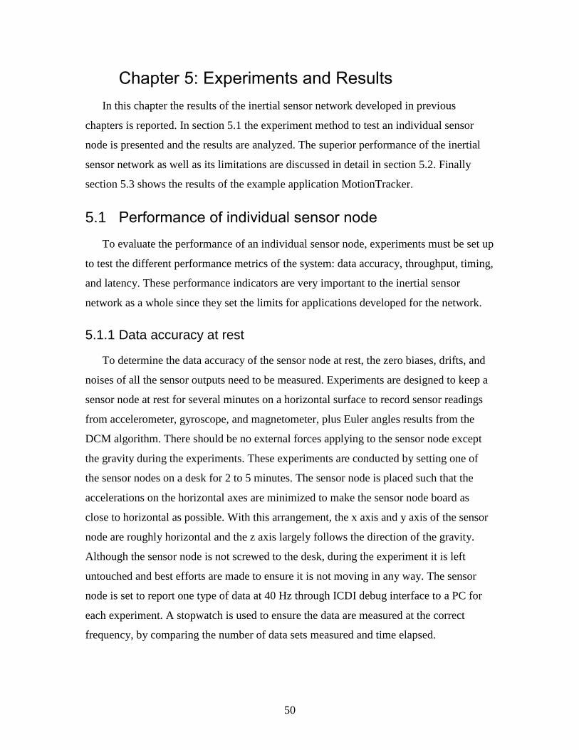
50

Chapter 5: Experiments and Results

In this chapter the results of the inertial sensor network developed in previous

chapters is reported. In section 5.1 the experiment method to test an individual sensor

node is presented and the results are analyzed. The superior performance of the inertial

sensor network as well as its limitations are discussed in detail in section 5.2. Finally

section 5.3 shows the results of the example application MotionTracker.

5.1 Performance of individual sensor node

To evaluate the performance of an individual sensor node, experiments must be set up

to test the different performance metrics of the system: data accuracy, throughput, timing,

and latency. These performance indicators are very important to the inertial sensor

network as a whole since they set the limits for applications developed for the network.

5.1.1 Data accuracy at rest

To determine the data accuracy of the sensor node at rest, the zero biases, drifts, and

noises of all the sensor outputs need to be measured. Experiments are designed to keep a

sensor node at rest for several minutes on a horizontal surface to record sensor readings

from accelerometer, gyroscope, and magnetometer, plus Euler angles results from the

DCM algorithm. There should be no external forces applying to the sensor node except

the gravity during the experiments. These experiments are conducted by setting one of

the sensor nodes on a desk for 2 to 5 minutes. The sensor node is placed such that the

accelerations on the horizontal axes are minimized to make the sensor node board as

close to horizontal as possible. With this arrangement, the x axis and y axis of the sensor

node are roughly horizontal and the z axis largely follows the direction of the gravity.

Although the sensor node is not screwed to the desk, during the experiment it is left

untouched and best efforts are made to ensure it is not moving in any way. The sensor

node is set to report one type of data at 40 Hz through ICDI debug interface to a PC for

each experiment. A stopwatch is used to ensure the data are measured at the correct

frequency, by comparing the number of data sets measured and time elapsed.

51

Figure 15 shows the raw readings (unit: m/𝑠2) for all 3 axes of accelerometer. The

vertical scale represents the accelerometer readings while the horizontal scale represents

the enumeration of samples for all graphs.

0

0.1

0.2

0.3

0.4

0.5

12

26

45

16

76

90

11

12

61

35

11

57

61

80

12

02

62

25

12

47

62

70

12

92

63

15

13

37

63

60

13

82

64

05

14

27

64

50

14

72

64

95

15

17

65

40

15

62

65

85

16

07

66

30

16

52

6Acc

ele

rati

on

(m

/𝑠^2

)

Samples

Accelerometer X

0

0.1

0.2

0.3

0.4

0.5

12

26

45

16

76

90

11

12

61

35

11

57

61

80

12

02

62

25

12

47

62

70

12

92

63

15

13

37

63

60

13

82

64

05

14

27

64

50

14

72

64

95

15

17

65

40

15

62

65

85

16

07

66

30

16

52

6Acc

ele

rati

on

(m

/𝑠^2

)

Samples

Accelerometer Y

9.2

9.3

9.4

9.5

9.6

9.7

12

26

45

16

76

90

11

12

61

35

11

57

61

80

12

02

62

25

12

47

62

70

12

92

63

15

13

37

63

60

13

82

64

05

14

27

64

50

14

72

64

95

15

17

65

40

15

62

65

85

16

07

66

30

16

52

6Acc

ele

rati

on

(m

/𝑠^2

)

Samples

Accelerometer Z

Figure 15: The accelerometer results for Sensor Node 2 when at rest on desk surface

52

After analyzing the raw data in Figure 15, the averages, standard deviations, noises

and the slopes of the readings for each axis are computed and presented in Table 8. The

slope for all axes are close to 0, indicating that the accelerometer results do not drift over

time. The noises data are calculated according to the following noise spectral density

formula:

𝑁0 =𝜎

√𝐵𝑊

In this formula, 𝜎 represents the standard deviation of the data, while BW represents

the frequency of the data. The noise density calculated for the x and y axes largely agree

with the noise density data in the specifications of the MPU9150 sensor (400 μg/√Hz).

Obviously, as depicted in Figure 15, the z axis is significantly noisier with a noise density

of 533.3 μg/√Hz. This is due to the physical structure of 3-axis accelerometer in the

MPU9150 chip. Often, for the horizontal axes, x and y, there are enough space in the

package to put metal beams that change capacitance when forces are applied along x and

y directions. For the z axis, the package is not high enough to allow the same structure as

x and y. Instead, a cantilever system is used, also changing the capacitance when forces

are applied along z axis. This structure, however, is usually noisier than the simple metal

beam structure. Therefore it is common that for many accelerometers, the z axis has more

noises than the x and y axes.

Table 8: The acceleration data for Sensor Node 2 when at rest on desk surface

X Y Z

Average (m/𝑠2) 0.3530 0.1563 9.496

Standard deviation

(m/𝑠2) 0.02061 0.01871 0.03305

Noises (μg/√Hz) 332.5 301.9 533.3

Slope 3.149E-09 -3.723E-08 -1.063E-06

53

Table 8 also shows that there exists a quite significant amount of zero biases and

possibly some linear biases in the accelerometer readings. The total acceleration, by

combining the accelerations from all 3 axes, is calculated to be 9.504 m/𝑠2, as opposed

to the gravity constant of approximately 9.81 m/𝑠2. Experiments on other sensor nodes

have yielded similar results. Therefore when using the acceleration data it is important to

calibrate the sensor node to remove zero biases and linear biases. Another error

contributing to these results is the tilt between the z axis and the direction of gravity.

However there is no way to perfectly place the sensor node so that the z axis could match

the direction of gravity exactly, hence there is always a small component of the gravity in

the x and y axes. Thus it is only possible to estimate the zero biases with the assumption

that the tilt is 0.

The gyroscope data appears to have better quality than the accelerometer data, as

shown in Figure 16, with very small range of fluctuation. And all 3 axes of the gyroscope

have equally good results. Same statistic values as accelerometer are calculated for

gyroscope measurements; they are shown below in Table 9. These data have much less

noises than the accelerometer, even though the numeric range is broader (250°/s vs 2g).

Similar to the accelerometer, there is no drift for the sensor since the slope is negligible.

As the sensor node is at rest, all the non-zero data are actually the zero-biases. The

averages of readings for different axes show that the x axis has a bigger zero bias than the

y and z axes. The existence of these zero biases, even though small, could still cause the

results to diverge after integration. Thus when using the raw gyroscope data, these values

should be deducted from the sensor outputs.

54

0.04

0.045

0.05

0.055

0.06

13

39

67

71

01

51

35

31

69

12

02

92

36

72

70

53

04

33

38

13

71

94

05

74

39

54

73

35

07

15

40

95

74

76

08

56

42

36

76

17

09

97

43

77

77

58

11

38

45

18

78

99

12

79

46

5

An

gula

r V

elo

city

(°

/s)

Samples

Gyroscope X

0

0.005

0.01

0.015

0.02

13

39

67

71

01

51

35

31

69

12

02

92

36

72

70

53

04

33

38

13

71

94

05

74

39

54

73

35

07

15

40

95

74

76

08

56

42

36

76

17

09

97

43

77

77

58

11

38

45

18

78

99

12

79

46

5

An

gula

r V

elo

city

(°

/s)

Samples

Gyroscope Y

0

0.005

0.01

0.015

0.02

13

39

67

71

01

51

35

31

69

12

02

92

36

72

70

53

04

33

38

13

71

94

05

74

39

54

73

35

07

15

40

95

74

76

08

56

42

36

76

17

09

97

43

77

77

58

11

38

45

18

78

99

12

79

46

5

An

gula

r V

elo

city

(°

/s)

Samples

Gyroscope Z

Figure 16: The gyroscope data for Sensor Node 2 when at rest on desk surface

55

Table 9: The gyroscope data for Sensor Node 2 when at rest on desk surface

X Y Z

Average (°/s) 0.05262 0.01556 0.01570

Standard deviation

(°/s) 0.0009901 0.0009297 0.0008129

Noises (°/s/√𝐻𝑧) 0.0001565 0.0001470 0.0001285

Slope -2.965E-08 -1.398E-08 1.912E-08

The magnetometer measurements have been conducted in a typical home

environment where electronic devices are present. Table 10 summarizes the

magnetometer readings in statistics.

Table 10: The Magnetometer results for Sensor Node 2 when at rest on desk surface

X Y Z

Average (μT) -8.416 22.43 49.44

Standard deviation

(μT) 0.8335 0.8296 0.8153

Noises (μT/√Hz) 0.1318 0.1312 0.1289

Slope -4.655E-06 -8.842E-06 -9.033E-06

Magnetometer data in Table 10 show that the magnetic field measurement are quite

stable when the sensor node is at rest and no major interference is near the sensor. The

slope is close to 0 and the noises are small compared to the magnitude of average

readings.

56

To evaluate the magnetometer’s accuracy, the sensor node is turned around on a

horizontal surface to find out the max and min values for x and y axes. It turns out that

the y axis value for Sensor Node 2 changes from close to 0 to more than 50, but never

becomes negative, while the x axis value measures more negative values than positive

values. This indicates that the magnetometer has significant zero biases. In the rotation of

the sensor node, the z axis stays roughly the same most of the time, as expected for

horizontal movements. The conclusion is that the magnetometer of the sensor node

cannot be trusted for calculating direction on its own in home and office environment.

The magnetometer should always be used with other sensors to compute a more reliable

heading.

An experiment to evaluate the accuracy of the Euler angle output of the sensor node

is also conducted. The Euler angles are calculated from measurements of accelerometer,

gyroscope, and magnetometer, hence the accuracy of the Euler angles largely depend on

the data input to the DCM algorithm. Since the accelerometer and gyroscope data both

demonstrate good accuracy at rest, the roll and pitch angles that depend on these results

are expected to be accurate. The yaw (heading) data, on the other hand, largely depend on

the magnetometer, which is proven to be unreliable. Therefore if the DCM algorithm has

reasonable performance, the roll and pitch data should be relatively accurate while the

yaw data may have more errors. Figure 17 shows the roll, pitch, and yaw angles of the

Euler angle output of the sensor node. The vertical scale shows the angles in degrees.

57

-1

-0.5

0

0.5

1

1 33

56

69

10

03

13

37

16

71

20

05

23

39

26

73

30

07

33

41

36

75

40

09

43

43

46

77

50

11

53

45

56

79

60

13

63

47

66

81

70

15

73

49

76

83

80

17

83

51

86

85

90

19

93

53

96

87

An

gle

(°

)

Samples

Euler Angle X (Roll)

270

272

274

276

278

280

282

13

35

66

91

00

31

33

71

67

12

00

52

33

92

67

33

00

73

34

13

67

54

00

94

34

34

67

75

01

15

34

55

67

96

01

36

34

76

68

17

01

57

34

97

68

38

01

78

35

18

68

59

01

99

35

39

68

7

An

gle

(°

)

Samples

Euler Angle Z (Yaw)

3

3.5

4

4.5

5

13

35

66

91

00

31

33

71

67

12

00

52

33

92

67

33

00

73

34

13

67

54

00

94

34

34

67

75

01

15

34

55

67

96

01

36

34

76

68

17

01

57

34

97

68

38

01

78

35

18

68

59

01

99

35

39

68

7

An

gle

(°

)

Samples

Euler Angle Y (Pitch)

Figure 17: The Euler angle data for Sensor Node 2 when at rest on desk surface

58

As Figure 17 shows, the roll and pitch angles are relatively stable, while the yaw

angle has a huge shift at around the 1000th sample. This is probably due to yaw angle is

almost solely computed with results from magnetometer when the sensor is stationary.

The MPU9150’s magnetometer could suffer from various magnetic disturbances

commonly found in home and office environment. This is probably one of cases that the

magnetic field changes in the environment since data in pitch and roll do not seem to

indicate a movement of the sensor node itself at the exact moment.

The statistics of the Euler angle results are presented in Table 11.

Table 11: The Euler Angle results for Sensor Node 2 when at rest on desk surface

X (Roll) Y (Pitch) Z (Yaw)

Average (°) -0.1935 4.012 276.1

Standard deviation (°) 0.05633 0.04215 0.9033

Slope -1.603E-07 -4.692E-07 -3.714E-05

Table 11 demonstrates the results computed by the DCM library provided by Texas

Instruments. The library function takes input from the raw accelerometer, gyroscope, and

magnetometer readings, without any filtering. The low standard deviations of roll and

pitch suggest that there are little noises in these results. However the yaw angle produces

much greater standard deviation than the other axis, because of the shift at around the

1000th sample. If the first 2000 samples are truncated, the yaw angle would have an

average angle of 276.0°, a standard deviation of 0.6995°, and a slope of -2.330E-06.

These results are still many times worse than the other axes.

5.1.2 Data accuracy while moving

Since the inertial network is designed to recognize or measure actions, it is important

to understand how well the sensor nodes perform in a moving situation. To test this, one

of the sensor nodes is mounted on a robotic arm with 6 degrees of freedom. In order to

simulate consumer usage, the sensor node is only tightly fasten to the robotic arm using

59

bandages, not permanently attached to it in any way. The sensor node is placed such that

the y-axis of the sensor node goes along the direction of the arm from the base to the top;

the x-axis goes sideway, vertical to the robotic arm; the z-axis goes into the robotic arm,

vertical to its top surface. The experiment lets the robotic arm moving constantly between

45 and 90 degrees, and the sensor node measures the movement using Euler angles. A

video camera is used to capture the movement. The results from the video camera are

compared with the sensor node results. In order to match the sensor data with the video

camera as closely as possible, the data rate for the sensor node is set at 50 Hz and the

frame rate for the video camera is set at 48Hz. The experiment shows that the robotic arm

overshoots a bit after reaching the target angle. Sometimes after overshooting the arm is

visibly shaking back and forth around the target angle. Therefore after each movement,

the robotic arm is programmed to wait for 5 seconds before moving back, so the arm

could stabilize over the period. A comparison is made between the peak data recorded by

the sensor node and the angle measured from the corresponding video frame. Similar

comparison is done with the stabilized data and its corresponding video frame as well.

60

In the experiment, the robotic arm moves from 90 degree position to 45 degree

position and back 3 times. Figure 18 shows the primary Euler angle results produced by

the sensor node attached to the robotic arm during this motion. The vertical scale shows

angle in degrees. The labelled data points have the format of (sample number, angle in

degrees). These angle values are compared to the measured angles from their

corresponding video frame. The video is captured by a video camera from the side of the

robotic arm. The original video has to go through a de-fisheye process to restore the

scene. Since the video is captured at 48 Hz, the frames do not have a 1-1 relation with the

results measured by the sensor node. The corresponding frames are found by going

through the video frame by frame and looking for the overshooting moments and the

stabilized moments of the robotic arm. Even so, the frames are captured at slightly

different times from their corresponding sensor measurements. But this difference should

not have any significant effect on the comparison.

Figure 18: Euler angle in X axis (roll, the main axis of motion) for robotic arm to

move between 90 and 45 degrees

30, 93.34328461

280, 33.85823822

482, 44.60715485

538, 101.3745117

731, 93.23204803

788, 37.98745728

1001, 44.93599319

1053, 102.8872528

1249, 93.15612793

1303, 37.77375412

1497, 45.12750244

1569, 102.8249512

1774, 93.1652832

0

20

40

60

80

100

120

0 200 400 600 800 1000 1200 1400 1600 1800 2000

An

gle

(°)

Samples

Euler Angle X (Roll)

61

Table 12 shows the comparison between the angle measured by the sensor node and

“pictured angle”, the angle captured by the video camera. By using “measure” tool in

GIMP image processing software on the robotic arm and the platform, relative angle to

the horizontal plane of the video frame can be found. The pictured angle is thus

calculated as the difference of the angle of the robotic arm and the angle of the platform.

The error is the difference between measured Euler angle around X-axis (roll) and the

pictured angle.

Table 12: Comparison between the angle measured by the sensor node and the

pictured angle on corresponding video frame (unit: degree)

Motor 2 Angle (°) Pictured Angle (°) Measured Angle X (°) Error (°)

90 94.66 93.34 -1.317

45- Overshoot 43.82 33.86 -9.962

45 45.4 44.61 -0.7929

90+ Overshoot 96.69 101.4 4.685

90 94.36 93.23 -1.128

45- Overshoot 45.54 37.99 -7.553

45 45.83 44.94 -0.8940

90+ Overshoot 96.69 102.9 6.197

90 94.42 93.16 -1.264

45- Overshoot 45.69 37.77 -7.916

45 45.83 45.13 -0.7025

90+ Overshoot 96.69 102.8 6.135

62

90 94.22 93.17 -1.055

Average Error 0.007238

Standard Deviation

Error 4.921

In Table 12, the angles measured by the sensor node and by the video frame are

compared in different situations. Each row of the data is corresponding to a data tag in

Figure 18 in sequence. It is obvious that in overshooting situation, the absolute

differences between two types of measurements increase significantly. Since the video

captured angle more or less represents the actual angle the sensor node should be

experiencing, the results indicate that the sensor node performs poorly in measuring Euler

angles when the motion is abrupt, probably due to high acceleration at the moment. This

is essentially a problem with the DCM algorithm and the weights of the algorithm for

accelerometer, gyroscope, and magnetometer. Aside from the overshooting data points,

the sensor node shows consistency in the other data points, with an error around -1

degree. This constant error is due to the positioning of the senor on the robotic arm and

the biases in measuring the angle from video frames. This means the sensor could

measure Euler angles in good accuracy and consistency if the motion is slow and gentle.

The Euler angle results in y-axis (pitch), and z-axis (yaw) are presented in Figure 19

and Figure 20 below.

63

30, -2.363996506

280, 0.883129001

482, -0.624213338

538, -2.300556898

731, -2.275129318

788, 0.579465568

1001, -0.684141994

1053, -2.21688509

1249, -2.157866001

1303, 0.540967822

1497, -0.638550282

1569, -2.311314344

1774, -2.279172421

-5

-4

-3

-2

-1

0

1

2

3

0 200 400 600 800 1000 1200 1400 1600 1800 2000

An

gles

(°

)

Samples

Euler Angle Y (Pitch)

Figure 19: Euler angle in Y axis (pitch, off-motion axis)

30, 233.161438

280, 196.2185516

482, 200.8597412

538, 232.6723938

731, 233.1469421

788, 200.8644104

1001, 201.931488

1053, 232.8510132

1249, 233.2621918

1303, 199.8334656

1497, 200.8834991

1569, 232.7128601

1774, 232.8855286

190

195

200

205

210

215

220

225

230

235

240

0 200 400 600 800 1000 1200 1400 1600 1800 2000

An

gle

(°)

Samples

Euler Angle Z (Yaw)

Figure 20: Euler angle in Z axis (yaw, off-motion axis)

64

Results in Figure 19 and Figure 20 suggest that, as the robot arm goes from 90 degree

to 45 degree, the pitch and yaw (heading) angles change at about the same pace as roll

angle. However, the Euler angle measurements of yaw are quite inaccurate as shown in

sub-section 5.1.1, so it is only reliable to look at roll and pitch. It should be noted that in

Figure 19 the pitch angle results seem to have a lot more noises than roll and yaw when

the robot arm is at move, the truth is the vertical scale of Figure 19 is much smaller than

the other two figures and all axes should have similar level of noises while the sensor

node is at move. The small changes of the pitch angle between 90-degree and 45-degree

position may represent the actual changes of the sensor orientation, since both values are

quite close to 0. However, without another form of measurement, it is impossible to tell

how much errors are there in the pitch angle measurements. The only conclusion is that

both pitch and roll angle have less noise when the robotic arm is not moving violently.

5.1.3 Data rate limitation for BLE

A sensor node has a limitation on the throughput of the sensor data over Bluetooth

Smart. This limitation is found when the receiving end could no longer receive as many

data packets as the sensor node collects from MPU9150. An experiment has been carried

out to determine the maximum data frequency of transmission between a single sensor

node and an Android device, a Galaxy Nexus smartphone. The sensor node is set to

transmit 12 bytes of data together in one write command every cycle. The 12 bytes of

data is constructed as a counter to count from 0 to 359 iteratively. When the Android

device receives a set of data from the sensor node, it records the time. After 5 minutes,

there is a long list of timestamps corresponding to the data. The periods between

transmissions can be found by subtracting the neighboring timestamps. Table 13

summarizes the statistics of the time periods between the arrivals of data packets.

Table 13: Periods between transmissions at receiving end for different data

transmission rate

Data rate (Hz) 100 200 250

65

Average period

(ms) 9.996 4.996 4.477

Standard deviation

of period (ms) 8.007 5.487 5.029

As Table 13 shows, the results are exceptionally good. Even at 200 Hz, the Android

device is able to pick up every single transmission over the whole experiment. The

average period is not exactly the same as 5 ms for 200 Hz experiment, because of the

slightly different clock between the sensor node and the smartphone. At 250 Hz, the

average period 4.477 ms is more than 20% larger than the expected period of 4 ms,

indicating that many samples are lost in transmission. Indeed, after checking the data

received, it is shown that 632 out of more than 60000 recordings are not consecutive with

previous data. This means there are at least 632 cases that a minimum of one data packet

is lost. If the data rate is pushed to 500 Hz (next frequency level) or more, the sensor

node would run for a while, and then freeze because the UART channel is jammed.

In addition, the large standard deviations also suggest that the data packets are not

arriving in uniform periods. By examining the data closely, it is found that most of the

time data packets are arriving at 1 or 2 milliseconds intervals, but occasionally there are

no data arriving for a large interval of nearly 100 ms. This means the time recorded when

the data packet arrives should not be used as if it is the actual time the data is collected.

The data rate limitation not only applies to the sensor node, but also to the device that

is receiving the data packets. It is found that, for 100 Hz and 200 Hz experiments, even

though there are no missing data packets with a Galaxy Nexus, there are many missing

packets with an Oneplus One. In fact, it is found that the Oneplus One is only able to

receive all packets if the data transfer rate is below 50 Hz. Due to the varying

specifications of consumer electronic devices, there is not a definite maximum working

frequency for the sensor node. Therefore a speed test is needed for all applications to

determine the maximum working data rate for any consumer devices.

66

5.1.4 Battery Life

It is found that a single 3.3V rechargeable coin battery of common brand could not

power the entire sensor node board. The primary reason is likely that the battery is unable

to keep the voltage at exactly 3.3V which is required by the microcontroller. The solution

of this problem is to use more powerful battery pack with output voltage higher than

3.3V. The battery pack should be connected to the sensor node power system before the

regulator, so the voltage could be adjusted to exactly 3.3V. A control circuit is needed for

the battery pack to be able to recharge when the sensor node is connected to a power

source using micro-USB cable.

5.2 Performance of inertial sensor network

When combining many sensor nodes into an inertial sensor network, these sensor

nodes need to connect with one single remote data processing device simultaneously. The

most important performance metric for the sensor network as a whole is the data

throughput, which is often limited by the implementation of the remote data processing

device. Normally, the more sensor nodes are connected, the less frequently each sensor

node is able to transmit the data due to congestion at the receiving end. In this

experiment, 4 sensor nodes are connected to a Galaxy Nexus and every one of them is

transmitting 12 bytes of data by BLE each cycle. The experiment runs for more than 10

minutes; it is set up in the same way as the experiment in sub-section 5.1.3. Whenever a

data packet arrives, the Galaxy Nexus records the timestamp as well as its origin node.

Table 14 shows the statistics of the periods between data packets from each sensor node.

Table 14: Transmission rate measured for 4 sensor nodes at receiving end

Node 1 Node 2 Node 3 Node 4

Average period (ms)

at 20 Hz 49.95 50.02 50.00 50.01

Standard deviation

period (ms) at 20 Hz 18.83 18.47 22.39 26.01

67

Average period (ms)

at 40 Hz 24.96 25.01 25.00 25.00

Standard deviation

period (ms) at 40 Hz 25.50 26.07 28.22 27.95

Average period (ms)

at 50 Hz 33.84 30.87 20.79 20.00

Standard deviation

period (ms) at 50 Hz 44.95 43.75 26.64 25.95

As Table 14 shows, when there are 4 sensor nodes connecting to the Android device

at the same time, the maximum working frequency is 40 Hz. At this frequency and lower,

the data packets from all sensor nodes are successfully received. For the 50 Hz case, data

from Node 1 and Node 2 are coming at significantly larger intervals than the Sensor 3

and Sensor 4. That is because at some instances these data are coming in at a very high

rate and the Galaxy Nexus is not able to handle them in time. Some data transmissions

from Node 1 and Node 2 are completely lost. If the number of sensor nodes is reduced,

then the system might not have this problem at the same frequency due to reduced

workload for the receiving smartphone. But if the number of sensor nodes is to increase,

then the maximum working frequency might be even lower than 40 Hz.

5.3 Results of MotionTracker PNS

The major source of errors for measuring motion, as discussed in sub-section 5.1.2, is

the overshoot of Euler angle results when the sensor is moving back and forth. Since the

step length is calculated by using the biggest difference between the displacements of the

two feet, it is guaranteed to suffer from overshoot errors. Although the overshoot error is

near constant when the motion has a definite pattern, the pedestrian walking pattern is

more random and therefore harder to estimate the error. Hence in the experiment the

subject tries to be slow and gentle while stepping, so the overshoot error could be

minimized. The sensor may also suffer from errors due to muscle movement during a

68

step when attached to the legs. The biggest impact of this type error happens when the

user is standing still, the error may cause the system to think the user has actually started

walking. Therefore it is important to have a sufficiently large step threshold ES to prevent

this problem.

The sensor nodes are placed in front of the subject’s legs adjacent to the knees,

keeping the y-axis aligned with the front surface of the legs towards top. There is an

initial position error: the initial horizontal displacement of either foot may not equal to 0.

Since the step length takes the difference of the displacements, the error is mostly

cancelled out, and only the error due to the difference in positioning of the sensors on two

legs remains. Efforts are made to ensure the roll measurements from corresponding

sensors on the two legs are as close to 0 as possible when the user is standing still.

The experiment is carried out indoor. The experiment is done with all sensor nodes

powered by USB wires connecting to a PC, so the maximum walking distance for the

experiment is limited. Using the tiles on floor, 6 parallel lines, each separated by 0.36

meter distance from another, are marked. The subject starts at one end and walks through

the 1.8 meter distance with 5 steps, hitting the marked lines exactly. When the subject

makes a mistake, such as missing the line, or step backwards, the trial ends and results

are abandoned. Sometimes even if the subject performs perfectly, the trials can also

produce bad results that have to be discarded. After inspecting these results it is found

that counting extra steps can significantly inflate the total distance travelled. Further

investigation shows that sometimes the step threshold ES is too small to contain the

fluctuations in Euler angles, causing the system to count a non-existent step with a step

length slightly greater than ES. In some very rare cases, the system can miss a step when

counting, therefore underestimating the total distance. Table 15 below shows the results

of the experiment. In the first 3 trials, the subject starts stepping with left leg; in Trial 4

and Trial 5, the subject starts stepping with right leg.

69

Table 15: MotionTracker experiment results with step by step measurements.

Step 1 2 3 4 5

Actual Distance (m) 0.36 0.72 1.08 1.44 1.8

Trial 1

Left leg

first

Results (m) 0.35 0.59 0.98 1.26 1.73

Percentage

Errors -2.78% -18.06% -9.26% -12.50% -3.89%

Trial 2

Left leg

first

Results (m) 0.47 0.85 1.34 1.63 1.92

Percentage

Errors 30.56% 18.06% 24.07% 13.19% 6.67%

Trial 3

Left leg

first

Results (m) 0.37 0.89 1.2 1.48 1.83

Percentage

Errors 2.78% 23.61% 11.11% 2.78% 1.67%

Trial 4

Right leg

first

Results (m) 0.32 0.61 0.88 1.26 1.67

Percentage

Errors -11.11% -15.28% -18.52% -12.50% -7.22%

Trial 5

Right leg

first

Results (m) 0.29 0.66 0.96 1.44 1.76

Percentage

Errors -19.44% -8.33% -11.11% 0.00% -2.22%

The results in Table 15 show that no matter which leg the subject starts stepping with,

the final results after 5 steps are within 10% range of the actual distance. In the first 3

steps there are some great discrepancy between measured distance and actual distance,

but the difference narrows later in step 4 and 5. This is because the inaccuracy in the

model and the randomness of the legs’ movements during a step magnifies the error when

70

there are very few steps. The error becomes less significant in proportion as the number

of steps and the total distance grow. Still it represents the primary error for the

MotionTracker system. Better modelling, including more accurate numbers for the limb

lengths and adjustments for the position of the sensors, could estimate these errors and

improve the accuracy for the system.

71

Chapter 6: Conclusion and Future Work

Inertial sensor networks have a huge potential for consumer-oriented applications,

such as action capture, personal navigation, and consumer robotic control. As the MEMS

sensors become increasingly accurate and the wireless communication becomes more

efficient, inertial sensor networks are becoming an important supplement to mobile

devices. The current inertial sensor networks are often designed for a specific application

and thus lack the compatibility needed for consumer products. Therefore it is desired to

have a low-cost open-source development platform which is compatible with most of

today’s consumer electronic devices.

6.1 Conclusions

The inertial sensor network developed in this thesis tries to fulfill this need by using

low-cost sensors for measurements and Bluetooth Smart technology for transmission.

Compared to other common wireless transmission protocols such as Wi-Fi and classic

Bluetooth, Bluetooth Smart technology consumes less power. Bluetooth Smart is also

supported by most modern personal mobile computing devices such as smartphones,

tablets, and laptop PCs. With limitations of unit price and physical size, the system aims

to achieve reasonable accuracy, data rate, and battery life for a range of applications.

Each sensor node of the prototype system takes input from a 9-axis MEMS sensor, which

produces acceleration, angular velocity, and magnetic field measurements. With the

sensor fusion algorithm, it is possible to calculate Euler angles, Quaternions, and rotation

matrices real-time. Such a large set of data allow many possibilities in applications. The

data are transmitted to a microcontroller on the sensor node board. This microcontroller is

equipped with capabilities to do a large amount of floating point calculations real-time,

allowing it to process the sensor results on the run, such as applying filters, removing

biases, or estimating errors. This feature is essential since the bandwidth of the Bluetooth

Smart is precious and reducing the amount of data for transmission can improve the

maximum data rate. The processed and selected data are then sent over to the Bluetooth

Smart module for transmission to the remote data processing device, where the data from

all sensor nodes are synthesized and analyzed for applications.

72

A simple personal navigation system is designed to demonstrate the application of the

inertial sensor network. The concept of this PNS is based on measuring the tilt of the legs

when walking, rather than integrating the accelerations. Four sensor nodes are placed just

above and below knees of a user. An Android app is developed to collect data from all

the sensor nodes and interface with the user. Once all the sensor nodes are connected, the

app commands all nodes to start automatically transmitting Euler angles to the device

when new values are measured. The app calculates step length from these angles when

the two feet are furthest from each other. The step lengths are accumulated to produce the

total distance travelled by the user. These results are displayed to the user during the

process.

A series of experiments are conducted to test the performance of an individual sensor

node. The results suggest that the sensor node produces good outputs for accelerometer

and gyroscope when at rest. The Euler angle results calculated based the raw sensor

inputs and the DCM library are also quite accurate. However the magnetometer of

MPU9150 cannot produce measurements accurate enough to determine the orientation in

home or office environment. When the sensor node is moving, the accuracy of the data

drops. As the sensor node experiences large acceleration shock, the Euler angle could

produce exaggerated results and only stabilize after a few seconds. The data rate of the

sensor node is limited by the communication between the microcontroller and the

BLE113 module. It is found that the communication between a sensor node and a Galaxy

Nexus could work without missing data packets at a maximum frequency of 200 Hz.

When there are 4 sensor nodes forming the inertial sensor network, the maximum

data rate is limited by the remote data processing device. Using a Galaxy Nexus with

Android system to receive the sensor node transmission, the maximum working

frequency found in the experiment is 40Hz. This data rate should be good enough for

many applications targeting consumer market.

An evaluation is also conducted for the MotionTracker example application. It is

found that the distance estimated by the system has an error of roughly 10%.

73

6.2 Future work on the inertial sensor network

The inertial sensor network is designed to be an open-source development platform

for consumer oriented applications. We hope developers of wearable sensor network

applications can utilize this platform. Still the system could be improved in various ways

to enable more potential applications on the platform.

First of all the sensor nodes need to have a working on-board battery system. The

3.3V rechargeable coin battery in hardware design is proved to be insufficient to power

the whole sensor node alone. Potentially an additional same coin battery could solve the

issue, but it would significantly increase the physical size of a sensor node. An ideal

solution would be to replace the coin battery with a rechargeable battery pack. This type

of battery pack could hold more energy than the coin battery and thus could last longer. A

control circuit is needed to for recharging the battery pack when micro-USB cable is

connected. The battery pack should be connected to the voltage regulator to output

consistent 3.3V voltage. Since the battery pack is rechargeable, it does not have to be

exposed to allow replacements. Hence the battery could be removed from the surface of

the board, reducing the physical size of the sensor node.

Another improvement could be done by further reducing the size of the sensor node

board. As a prototype, all functionalities of the sensor node are currently placed on a

single board for convenience. This has made the board unnecessarily large. As discussed

in sub-section 3.1.5, the components could be placed on both sides of the board, and

power-related components such as the regulator could be moved out of the main board.

This way the sensor node could become two separate boards. The one with the sensor,

microcontroller, and BLE module, has to be placed accurately for measurement; the other

with the battery and power components can be placed anywhere that is comfortable for

users.

Future developments of the system could first focus on improving the bottleneck that

is limiting the performance of the system as a whole. The main bottleneck for the

maximum data collection frequency is the remote data processing device that is receiving

the data. Since the remote data processing device should be a consumer electronic device,

74

its throughput improvements could come with the release of newer generations. On the

other hand, if the amount of data required to transmit each cycle is reduced, the

maximum data rate could increase. Developers of applications could try to use as few

bytes of data as possible to transmit the results from sensor nodes to the remote data

processing device.

Also, more complicated filters and error estimating algorithms could be deployed to

the microcontroller of the sensor nodes. These algorithms should be application-specific

with different assumptions for different scenarios. It is possible to significantly improve

data quality with algorithms like Zero Velocity Update, Optimal bias estimation, and

Kalman Filter.

As the MEMS technology improves, sensors with better accuracy and battery life

could become available at a lower price. Inertial sensor network is going to see increasing

penetration into everyday life of common people. The inertial sensor network prototype

discussed in this thesis attempts to help the efforts of developing consumer-centered

applications based on inertial sensors. The system could be updated with more accurate

sensor and more efficient wireless communication protocol in the future, allowing a

wider range of potential applications.

75

Reference

[1] R. Nerino, L. Contin, W. J. Gonçalves da Silva Pinto, G. Massazza, M. Actis, P.

Capacchione, A. Chimienti and G. Pettiti, "A BSN based service for post-surgical

knee rehabilitation," in Proceedings of the 8th International Conference on Body

Area Networks, Brussels, Belgium, Belgium, 2013.

[2] R. Slyper and J. K. Hodgins, "Action capture with accelerometers," in Proceedings

of the 2008 ACM SIGGRAPH/Eurographics , Vienna, Austria, 2008.

[3] J. C. Alvarez, D. Alvarez, A. López and R. C. González, "Pedestrian navigation

based on a waist-worn inertial sensor," Sensors, vol. 12, no. 8, pp. 10536-10549,

2012.

[4] R. Aylward and J. A. Paradiso, "A compact, high-speed, wearable sensor network

for biomotion capture and interactive media," in Proceedings of the 6th

international conference on Information processing in sensor networks, New

York, NY, USA, 2007.

[5] R. Feliz, E. Zalama and J. Gómez, "Pedestrian tracking using inertial sensors,"

Journal of Physical Agents, vol. 3, no. 1, pp. 35-43, 2009.

[6] K. Abdulrahim, C. Hide, T. Moore and C. Hill, "Using constraints for shoe

mounted indoor pedestrian navigation," Journal of Navigation, vol. 65, no. 1, pp.

15-28, 2012.

[7] J.-l. Zhang, Y.-y. Qin and C.-b. Mei, "Shoe-mounted personal navigation system

based on," Journal of Chinese Inertial Technology, vol. 19, no. 3, pp. 253-256,

2011.

[8] "Wi-Fi Direct," [Online]. Available: http://www.wi-fi.org/discover-wi-fi/wi-fi-

direct.

76

[9] "ZigBee Specification Overview," [Online]. Available:

http://www.zigbee.org/Specifications/ZigBee/Overview.aspx.

[10] "A Look at the Basics of Bluetooth Technology," [Online]. Available:

http://www.bluetooth.com/Pages/Basics.aspx.

[11] D. Vlasic, R. Adelsberger, G. Vannucci, J. Barnwell, M. Gross, W. Matusik and J.

Popović, "Practical motion capture in everyday surroundings," ACM Transactions

on Graphics, vol. 26, no. 3, p. 35, 2007.

[12] S. Y. Cho and C. G. Park, "MEMS based pedestrian navigation system," Journal

of Navigation, vol. 59, no. 01, pp. 135-153, 2006.

[13] E. Foxlin, "Pedestrian tracking with shoe-mounted inertial sensors," IEEE

Computer Graphics and Applications, vol. 25, no. 6, pp. 38-46, 2005.

[14] S. K. Park and Y. S. Suh, "A zero velocity detection algorithm using inertial

sensors for pedestrian navigation systems," Sensors, vol. 10, no. 10, pp. 9163-

9178, 2010.

[15] Ö. Bebek, M. A. Suster, S. Rajgopal, M. J. Fu, X. Huang, M. C. Cavusoglu, D. J.

Young, M. Mehregany, A. J. V. D. Bogert and C. H. Mastrangelo, "Personal

navigation via high-resolution gait-corrected inertial measurement units," IEEE

Transactions on Instrumentation and Measurement, vol. 59, no. 11, pp. 3018-

3027, 2010.

[16] R. Stirling, J. Collin, K. Fyfe and G. Lachapelle, "An innovative shoe-mounted

pedestrian navigation system," in proceedings of European navigation conference

GNSS, 2003.

[17] Texas Instruments, "Technical Documents for TM4C12x MCUs," 6 2014.

[Online]. Available: http://www.ti.com/lit/pdf/spms376.

77

[18] E. R. Bachmann, I. Duman, U. Y. Usta, R. B. McGhee, X. P. Yun and M. J. Zyda,

"Orientation tracking for humans and robots using inertial sensors," Computational

Intelligence in Robotics and Automation, 1999. CIRA'99. Proceedings. 1999 IEEE

International Symposium on, pp. 187-194, 1999.

[19] R. Zhu and Z. Zhou, "A real-time articulated human motion tracking using tri-axis

inertial/magnetic sensors package," Neural Systems and Rehabilitation

Engineering, IEEE Transactions on, vol. 12, no. 2, pp. 295-302, 2004.

[20] Texas Instruments, "SensorTag," 2013. [Online]. Available:

http://www.ti.com/ww/en/wireless_connectivity/sensortag/index.shtml?DCMP=se

nsortag&HQS=sensortag-bn.

78

Appendices

A. Cost of components for a sensor node

The following table shows the list of components with costs, before tax and delivery

fees. Pin headers and buttons are not specifically listed, instead, they are grouped together

in “Other” category with an estimated cost of $5 per sensor node. The total component

cost of a sensor node before tax is $70.92.

Table 16: Complete list of component costs of a sensor node

Manufacture Manufacture Part Number Units Costs (CAD)

InvenSense MPU9150 1 $16.79

MPD BU2032SM-G 1 $0.95

Taiyo Yuden TMK212BJ474KD-T 3 $0.42

TDK C2012X5R2E222K085AA 1 $0.22

TDK C2012X5R2E103K125AA 5 $0.64

TDK C2012X5R1E105K125AA 3 $0.54

Taiyo Yuden TMK212BJ225KG-T 1 $0.24

Johanson 251R15S240JV4E 2 $0.78

Kemet C0805C100KBRACTU 2 $0.86

Hirose ZX62-AB-5PA(11) 1 $1.18

NXP PDTC114ET,215 3 $0.63

Yageo RC0805JR-070RL 10 $0.16

79

Yageo RC0805JR-0710KL 3 $0.36

Yageo RC0805JR-07330RL 4 $0.09

Panasonic ERJ-6GEYJ472V 2 $0.24

Yageo RC0805FR-071ML 1 $0.12

Texas Instruments TPS73633DRBR 1 $2.66

Abracon AB26TRB-32.768KHZ-T 1 $0.62

Texas Instruments TM4C123GH6PMTR 1 $14.02

Samsung CL21F104ZBCNNNC 7 $0.25

Abracon ABM3-16.000MHZ-B2-T 1 $1.20

Cree CLVBA-FKA-CA1D181BB7R3R3 1 $0.69

C&K Components JS202011SCQN 1 $0.51

Bluegiga BLE113-A-V1 1 $21.76

Other (buttons, pins headers) $5

Total $70.92

80

B. Source code for sensor node software

The source code is hosted at Github, link:

https://github.com/rodericus1987/Sensor-Node-Software

The root folder contains the source files for TM4C123GH6PM microcontroller.

These files need to be compiled with the software stack “Tivaware” provided by Texas

Instruments, using Code Composer Studio (v5 or newer). The software tools and library

could be downloaded from:

http://www.ti.com/tool/sw-ek-tm4c123gxl

To load the program, a TM4C Launchpad is needed. The Launchpad needs to connect

debug out pins (TCK, TMS, TDO, TDI) with the sensor node, and then connects to PC

with a microUSB wire. The sensor node should be powered and a common ground

should be established between the sensor node and the Launchpad.

The “uart_demo” folder contains the configuration files for BLE113. These

configuration files could only be compiled and updated to the Bluetooth Smart module

via Bluegiga software tools and a Texas Instruments’ CC debugger.

81

C. Source code for MotionTracker app

The source code is also hosted at Github, link:

https://github.com/rodericus1987/MotionTrackerApp

The project should be edited and compiled using Eclipse IDE with Android SDK

Tools. Follow the instructions below to load the program to an Android device:

a) Install the Eclipse ADT (with Android SDK Tools included) from

http://developer.android.com/sdk/index.html

b) Download project file from Github, import it to the Eclipse workspace

c) Connect to an Android device with USB debugging enabled, run or debug the

program

82

D. Schematics and PCB design files for the sensor node board

The schematics and PCB design files can be found in the following link:

https://github.com/rodericus1987/Sensor-Node-Software/tree/master/schematics