An Axiomatic Characterization of CausalCounterfactualsDavid Galles and Judea PearlCognitive Systems LaboratoryComputer Science DepartmentUniversity of California, Los Angeles, CA 90024galles@cs.ucla.edu judea@cs.ucla.eduAbstractThis paper studies the causal interpretation of counterfactual sentences using a mod-i�able structural equation model. It is shown that two properties of counterfactuals,namely, composition and e�ectiveness, are sound and complete relative to this inter-pretation, when recursive (i.e., feedback-less) models are considered. Composition ande�ectiveness also hold in Lewis's closest-world semantics, which implies that for recur-sive models the causal interpretation imposes no restrictions beyond those embodied inLewis's framework. A third property, called reversibility, holds in nonrecursive causalmodels but not in Lewis's closest-world semantics, which implies that Lewis's axiomsdo not capture some properties of systems with feedback. Causal inferences basedon counterfactual analysis are exempli�ed and compared to those based on graphicalmodels.Keywords: Causality, counterfactuals, interventions, structural equations, policy analy-sis, graphical models.1 IntroductionHow do scientists predict the outcome of one experiment from the results of other experimentsrun under totally di�erent conditions? Such predictions require us to envision what the worldwould be like under various hypothetical changes, namely to invoke counterfactual inference.Though basic to scienti�c thought, counterfactual inference cannot easily be formalized inthe standard languages of logic, algebraic equations, or probability. The formalization ofcounterfactual inference requires a language within which changes occurring in the worldare distinguished from changes of one's beliefs about the world, and such distinction is notsupported by standard algebras, including the algebra of equations, Boolean algebra, andprobability calculus.Lewis (1973b) has proposed a logic of counterfactuals based on the notion of closestworlds: A sentence of the form \If A were the case, then B would be the case" is true1

in a world w just in case B is true in the closest world to w in which A is true. Thisframework presupposes the existence of a measure of distance between worlds that can beused to identify the closest A-world to w, for any world w and any sentence A in thelanguage of discourse. Lewis is careful to keep his formalism as general as possible, and, savefor the obvious requirement that every world be closest to itself, he does not impose anyspeci�c structure on the distance measure. However, the fact that people communicate withcounterfactuals suggests that they share a distance measure that is encoded parsimoniouslyin the mind. What mental representation is used for encoding those inter-world distances?Lewis himself provides a clue, the closest worlds that he envisions are causal in nature.For instance, when Lewis considers as an example a hypothetical world in which kangarooshave no tails, he argues that not just the state of the tail, but also the tracks that the animalmade, the animal's balance, and a variety of other factors would also be di�erent. Thus,Lewis appeals to our common knowledge of cause and e�ect in laying out which factors areexpected to change in the hypothetical world, and which factors are expected to be unaltered.If our assessment of inter-world distances comes from causal knowledge, the questionarises whether that knowledge does not impose its own structure on distances, a structurethat is not captured in Lewis's logic. Phrased di�erently, by agreeing to measure closestworlds on the basis of causal relations, do we restrict the set of counterfactual statements weregard as valid? The question is not merely theoretical. For example, Gibbard and Harper(1981) characterize decision-making conditionals, namely, sentences of the form \If we do A,then B," using Lewis's general framework, while Pearl (1994, 1995) constructs a calculus ofaction based directly on causal semantics, and whether the two formalisms are identical isuncertain.1Another application occurs in statistics. Rubin (1974), Holland (1986), and Robins (1986)all used counterfactual variables to analyze the e�ectiveness of treatments in clinical studies.Starting with the primitive notion of potential response Y (x; u) (read: the value that theresponse variable Y would have attained in patient u had the treatment been x), whichis treated as a random variable, they ask under what conditions one can infer the averagetreatment e�ect Eu[Y (x; u)] from clinical data (Typical conditions require that the treatmentassignment be randomized or semi-randomized.) Although the logic underlying this type ofanalysis has not been stated formally, statisticians use the closest-world framework as aguiding paradigm and have adopted certain rules of inference that plausibly follow from thisframework. For example, among their most commonly employed rules is the implication(called consistency [Robins, 1987]):X = x =) Y (x; u) = Y (u) (1)which states that the potential response of patient u to a hypothetical treatment x, Y (x; u),must coincide with the patient's observed response, Y (u), whenever the actual treatment Xhappened to be x. This rule, as we shall see, is a special case of an axiom of counterfactualscalled composition (see Eq. (17)), an axiom that follows from the requirement that the actualworld be closer to itself than any world that di�ers from the actual world.1Winslett (1988) and Ginsberg and Smith (1987) have also advanced theories of actions based on closest-world semantics, while Katsuno and Mendelzon (1991) have used this semantics to characterize belief up-dating. None of these assumes a special structure for the distance measure, to re ect causal considerations.2

The question remains, however, whether inference rules beyond Lewis's axioms are nec-essary for statisticians to fully and accurately capture the causal structure of the clinicaltest environment and the causal character of the counterfactuals considered in such an en-vironment. This paper analyzes this question for both recursive and nonrecursive causalmodels, namely, models of systems without and with feedback. We �rst show that Lewis'saxioms, together with the assumption of recursiveness, are sound and complete with respectto the causal interpretation of counterfactual, that is, causality per se imposes no restrictionsbeyond those embodied in the closest-world framework together with recursiveness. Whenwe consider nonrecursive systems, however, Lewis's axioms are not complete. We show thata property called reversibility holds in nonrecursive causal models yet it does not follow fromLewis's axioms. Thus, Lewis's framework misses some properties of causality in the generalcase of feedback systems in equilibrium.Section 2 gives a brief overview of causal models employing modi�able structural equa-tions and illustrates their use in the interpretation of causal and counterfactual utterances.Section 3 de�nes the properties of composition, e�ectiveness, and reversibility, and showsthat composition and e�ectiveness are sound and complete for recursive causal models, wherereversibility holds trivially. Section 4 compares causal models to Lewis's framework, and �ndsthat composition and e�ectiveness are sound in that formalism as well. Section 5 illustratesthe derivation of probabilistic answers to counterfactual queries using only composition ande�ectiveness as rules of inferences. Section 6 concludes with remarks on the role of counter-factual calculus vis a vis structural equations and graphs.2 Causal Models2.1 De�nitionsA causal model is a mathematical object that provides an interpretation (and e�ective com-putation) of every causal query about the domain. Following [Pearl, 1995a], we adopt herea construct named modi�able structural equations, that generalizes most causal models usedin engineering, biology, and economics.De�nition 1 (causal model) A causal model is a tripleM = < U; V; F >where(i) U is a set of variables, called exogenous, that are determined by factors outside the model.(ii) V is a set fV1; V2; : : : ; Vng of variables, called endogenous, that are determined by vari-ables in the model.(iii) F is a set of functions ff1; f2; : : : ; fng where each fi is a mapping from U [ (V n Vi) toVi such that F de�nes a mapping from U to V . (i.e., F has a unique solution for eachstate u in the domain of U). Symbolically, F can be represented by writingvi = fi(pai; u) i = 1; : : : ; n3

where pai is any realization of the (unique) set of variables PAi in V=Vi (connotingparents) that renders fi nontrivial.Every causal model M can be associated with a directed graph, G(M), in which each nodecorresponds to a variable in V and the directed edges point from members of PAi towardVi. We call such a graph, the causal graph associated with M . This graph merely identi�esthe endogenous variables PAi that have direct in uence on each Vi but it does not specifythe functional form of fi.De�nition 2 (submodel) Let M be a causal model, X be a set of variables in V , and x bea particular realization of X. A submodel Mx of M is the causal modelMx = < U; V; Fx >where Fx = ffi : Vi 62 Xg [ fX = xg (2)In words, Fx is formed by deleting from F all functions fi corresponding to members of Xand replacing them with the set of functions X = x. Implicit in the de�nition of submodelsis the assumption that Fx possesses a unique solution for every u.Submodels are useful for representing the e�ect of local actions and changes. If weinterpret each function fi in F as an independent physical mechanism and de�ne the actiondo(X = x) as the minimal change inM required to make X = x hold true under any u, thenMx represents the model that results from such a minimal change, since it di�ers fromM byonly those mechanisms that directly determine the variables in X. The transformation fromM to Mx modi�es the algebraic content of F , which is the reason for choosing the namemodi�able structural equations.De�nition 3 (e�ect of action) Let M be a causal model, X be a set of variables in V , andx be a particular realization of X. The e�ect of action do(X = x) on M is given by thesubmodel Mx.2De�nition 4 (potential response) Let Y be a variable in V , and let X be a subset of V . Thepotential response of Y to action do(X = x), denoted Yx(u), is the solution for Y of the setof equations Fx.We will con�ne our attention to actions in the form of do(X = x). Conditional actions,of the form \do(X = x) if Z = z" can be formalized using the replacement of equations,rather than their deletion [Pearl, 1994]. We will not consider disjunctive actions, of the form\do(X = x or X = x0)", as these complicate the probabilistic treatment of counterfactuals.2Readers that are disturbed by the impracticality of some local actions (e.g., creating a world where kanga-roos have no tails) are invited to replace the word \action" with the word \modi�cation" (see [Leamer, 1985]).The advantages of using hypothetical external interventions to convey the notion of \local change" are em-phasized in [Pearl, 1995a, p. 706]. 4

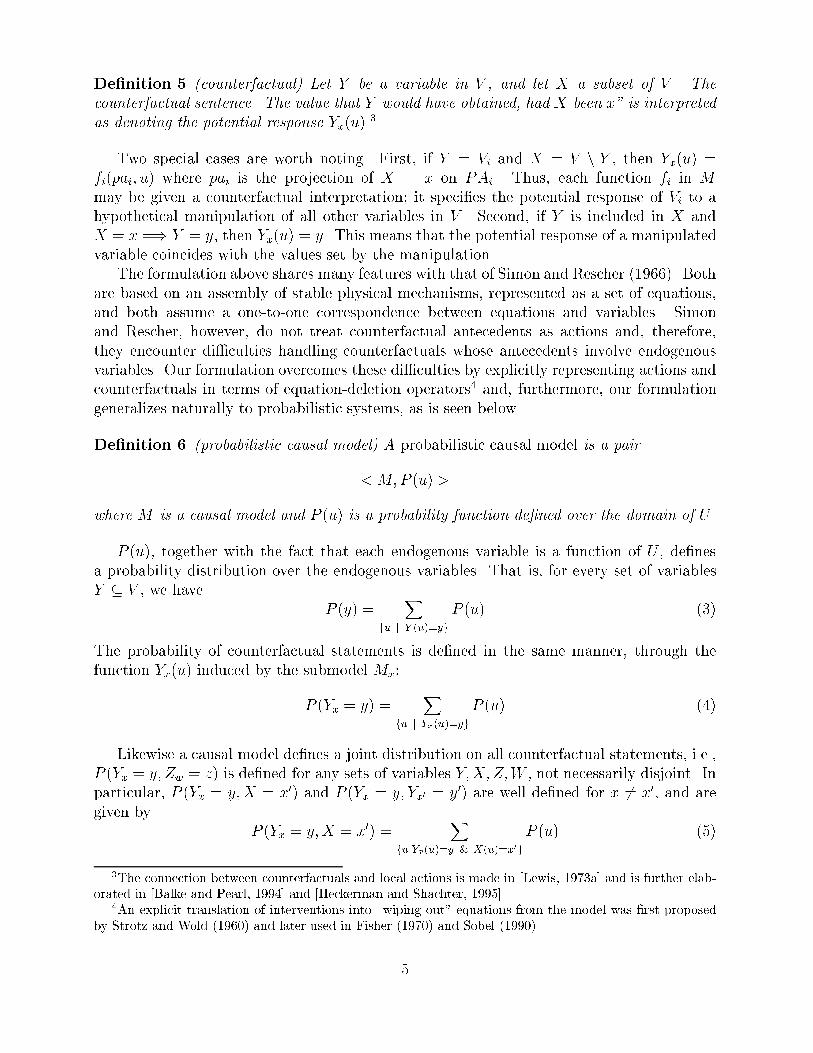
De�nition 5 (counterfactual) Let Y be a variable in V , and let X a subset of V . Thecounterfactual sentence \The value that Y would have obtained, had X been x" is interpretedas denoting the potential response Yx(u).3Two special cases are worth noting. First, if Y = Vi and X = V n Y , then Yx(u) =fi(pai; u) where pai is the projection of X = x on PAi. Thus, each function fi in Mmay be given a counterfactual interpretation; it speci�es the potential response of Vi to ahypothetical manipulation of all other variables in V . Second, if Y is included in X andX = x =) Y = y, then Yx(u) = y. This means that the potential response of a manipulatedvariable coincides with the values set by the manipulation.The formulation above shares many features with that of Simon and Rescher (1966). Bothare based on an assembly of stable physical mechanisms, represented as a set of equations,and both assume a one-to-one correspondence between equations and variables. Simonand Rescher, however, do not treat counterfactual antecedents as actions and, therefore,they encounter di�culties handling counterfactuals whose antecedents involve endogenousvariables. Our formulation overcomes these di�culties by explicitly representing actions andcounterfactuals in terms of equation-deletion operators4 and, furthermore, our formulationgeneralizes naturally to probabilistic systems, as is seen below.De�nition 6 (probabilistic causal model) A probabilistic causal model is a pair< M;P (u) >where M is a causal model and P (u) is a probability function de�ned over the domain of U .P (u), together with the fact that each endogenous variable is a function of U , de�nesa probability distribution over the endogenous variables. That is, for every set of variablesY � V , we have P (y) = Xfu j Y (u)=ygP (u) (3)The probability of counterfactual statements is de�ned in the same manner, through thefunction Yx(u) induced by the submodel Mx:P (Yx = y) = Xfu j Yx(u)=ygP (u) (4)Likewise a causal model de�nes a joint distribution on all counterfactual statements, i.e.,P (Yx = y; Zw = z) is de�ned for any sets of variables Y;X; Z;W , not necessarily disjoint. Inparticular, P (Yx = y;X = x0) and P (Yx = y; Yx0 = y0) are well de�ned for x 6= x0, and aregiven by P (Yx = y;X = x0) = XfujYx(u)=y & X(u)=x0gP (u) (5)3The connection between counterfactuals and local actions is made in [Lewis, 1973a] and is further elab-orated in [Balke and Pearl, 1994] and [Heckerman and Shachter, 1995].4An explicit translation of interventions into \wiping out" equations from the model was �rst proposedby Strotz and Wold (1960) and later used in Fisher (1970) and Sobel (1990).5

and P (Yx = y; Yx0 = y0) = Xfu j Yx(u)=y & Yx0(u)=y0gP (u): (6)When x and x0 are incompatible, Yx and Yx0 cannot be measured simultaneously, and itmay seem meaningless to attribute probability to the joint statement \Y would be y ifX = xand Y would be y0 if X = x0." Such concerns have been a source of objections to treatingcounterfactuals as jointly distributed random variables [Dawid, 1997]. The de�nition of Yxin terms of submodels di�uses such objections and further illustrates that joint probabilitiesof counterfactuals can be encoded rather parsimoniously using P (u) and F .2.2 ExamplesNext we demonstrate the generality of the modi�able structural equation model using twofamiliar applications: evidential reasoning and policy analysis. Additional applications in-volving the formalization of causal relevance and the interpretation of causal utterances canbe found in [Galles and Pearl, 1997b].2.2.1 Sprinkler Example������ @@RX1 SEASON@@R����X3SPRINKLER ������X2 RAIN����X4 WET?����X5 SLIPPERY

Figure 1: Causal graph illustrating causal relationships among �ve variables.Figure 1 is a simple yet typical causal graph used in common sense reasoning. It describesthe causal relationships among the season of the year (X1), whether rain falls (X2) duringthe season, whether the sprinkler is on (X3) during the season, whether the pavement is wet(X4), and whether the pavement is slippery (X5). All variables in this graph except the rootvariable X1 take a value of either \True" or \False." X1 takes one of four values: \Spring,"\Summer," \Fall," or \Winter." Here, the absence of a direct link between, for example,X1 and X5, captures our understanding that the in uence of the season on the slipperiness6

of the pavement is mediated by other conditions (e.g., the wetness of the pavement). Thecorresponding model consists of �ve functions, each representing an autonomous mechanism:x1 = u1x2 = f2(x1; u2)x3 = f3(x1; u3)x4 = f4(x3; x2; u4)x5 = f5(x4; u5) (7)The disturbances U1; : : : ; U5 are not shown explicitly in Figure 1 but are understood to governthe uncertainties associated with the causal relationships. The causal graph coincides withthe Bayesian network [Pearl, 1988] associated with P (x1; : : : ; x5) whenever the disturbancesare assumed to be independent, Ui k U n Ui. When some disturbances are judged tobe dependent, it is customary to encode such dependencies by augmenting the graph withdouble-headed arrows, as shown in Figure 3, Section 5.A typical speci�cation of the functions ff1; : : : ; f5g and the disturbance terms is givenby the Boolean model below:x2 = [(X1 = Winter) _ (X1 = Fall) _ ab2] ^ :ab02x3 = [(X1 = Summer) _ (X1 = Spring) _ ab3] ^ :ab03x4 = (x2 _ x3 _ ab4) ^ :ab04x5 = (x4 _ ab5) ^ :ab05 (8)where xi stands for Xi = true, and abi and ab0i stand, respectively, for triggering and in-hibiting abnormalities. For example, ab4 stands for (unspeci�ed) events that might causethe pavement to get wet (x4) when the sprinkler is o� (:x2) and it does not rain (:x3) (e.g.,pouring a pail of water on the pavement), while :ab04 stands for (unspeci�ed) events thatwill keep the pavement dry in spite of the rain (x3), the sprinkler (x2), and ab4 (e.g., coveringthe pavement with a plastic sheet).To represent the action \turning the sprinkler ON," or do(X3 = ON), we replace theequation x3 = f3(x1; u3) in the model of Eq. (7) with the equation x3 = ON. The resultingsubmodel,MX3=ON, contains all the information needed for computing the e�ect of the actionon the other variables. Thus, the operation do(X3 = ON) stands in marked contrast to thatof �nding the sprinkler ON; the latter involves making the substitution without removing theequation for X3, and therefore may potentially in uence (the belief in) every variable in thenetwork. In contrast, the only variables a�ected by the action do(X3 = ON) are X4 and X5,that is, the descendants of the manipulated variable X3. This mirrors indeed the di�erencebetween seeing and doing: after observing that the sprinkler is ON, we wish to infer that theseason is dry, that it probably did not rain, and so on; no such inferences should be drawnin evaluating the e�ects of the contemplated action \turning the sprinkler ON."This distinction obtains a vivid symbolic representation in cases where the Ui's are as-sumed independent, because the joint distribution of the endogenous variables then admitsthe product decomposition:P (x1; x2; x3; x4; x5) = P (x1)P (x2jx1)P (x3jx1)P (x4jx2; x3)P (x5jx4) (9)7

Similarly, the joint distribution associated with the submodel Mx representing the actiondo(X3 = ON) is obtained from the product above by deleting the factor P (x3jx1) andsubstituting X3 = ON:P (x1; x2; x4; x5jdo(X3 = ON)) = P (x1) P (x2jx1) P (x4jx2; X3 = ON) P (x5jx4) (10)The di�erence between the action do(X3 = ON) and the observation X3 = ON is thusseen from the corresponding distributions. The former is represented by Eq. (10), while thelatter by conditioning Eq. (9) on the observation; i.e.,P (x1; x2; x4; x5jX3 = ON) = P (x1) P (x2jx1) P (x3 = ONjx1)P (x4jx2; X3 = ON)P (x5jx4)P (X3 = ON)Note that the conditional probabilities on the r.h.s. of Eq. (10) are the same as thosein Eq. (9), and can therefore be estimated from pre-action observations. However, the pre-action distribution P is not su�cient for evaluating conditional counterfactuals wheneverthe conditions given are a�ected by the counterfactual antecedent. For example, the prob-ability that \the pavement would continue to be slippery once we turn the sprinkler o�,"tacitly presuming that currently the pavement is slippery, cannot be evaluated from the con-ditional probabilities P (xijpai) alone; the functional forms of the fi's (Eq. 7) are necessaryfor evaluating such queries [Balke and Pearl 1994; Pearl 1996].2.2.2 Policy Analysis in Linear Econometric ModelsCausal models are often used to predict the behavior of systems in dynamic equilibrium. Inthe economic literature, for example, we �nd the system of equationsq = b1p+ d1i+ u1 (11)p = b2q + d2w + u2 (12)where q is the quantity of household demand for a product A, p is the unit price of productA, i is household income, w is the wage rate for producing product A, and u1 and u2represent error terms, namely, unmodeled factors that a�ect quantity and price, respectively[Goldberger, 1992].This system of equations constitutes a causal model (De�nition 1) if we de�neV = fQ;Pg; U = fU1; U2; I;Wg and assume that each equation represents an autonomousprocess in the sense of De�nition 3. The causal graph of this model is shown in Figure 2.It is normally assumed that I and W are known, while U1 and U2 are unobservable andindependent in I and W . Since the error terms U1 and U2 are unobserved, the model mustbe augmented with the distribution of these errors, which is usually taken to be a Gaussiandistribution with the covariance matrix �ij = cov(ui; uj).We can use this model to answer queries such as:1. Find the expected value of the demand (Q) if the price is controlled at P = p0.2. Find the expected value of the demand (Q) if the price is reported to be P = p0.8

Q P

I WU1 U2

Figure 2: Causal graph illustrating the relationship between supply and demand3. Given that the current price is P = p0, �nd the expected value of the demand (Q) hadthe price been controlled at P = p1.To �nd the answer to the �rst query, we replace Eq. (12) with p = p0, leavingq = b1p+ d1i + u1 (13)p = p0 (14)The demand is then q = b1p0 + d1i+ u1, and the expected value of Q can be obtained fromi and the expectation of U1, givingE[Qjdo(P = p0)] = E[Q] + b1(p� E[P ]) + d1(i� E[I]):The answer to the second query is given by conditioning Eq. (11) on the current obser-vation fP = p0; I = i;W = wg and taking the expectation,E[Qjp0; i; w] = bip0 + d1i + E[U1jp0; i; w]: (15)The computation of E[U1jp0; i; w] is a standard procedure once �ij is given [Meditch, 1969].Note that, although U1 was assumed independent of I and W , this independence no longerholds once P = p0 is observed. Note also that Eqs. (11) and (12) both participate inthe solution and that the observed value p0 will a�ect the expected demand Q (throughE[U1jp0; i; w]) even when b1 = 0, which is not the case in query 1.The third query requires the conditional expectation of the counterfactual quantity Qp=p1,given the current observations fP = p0; I = i;W = wg, namely,E[Qp=p1jp0; i; w] = b1p1 + d1i+ E[U1jp0; i; w] (16)The expected value E[U1jp0; i; w] is the same in the solutions to the second and third queries;the latter di�ers only in the term b1p1. A general method for solving such counterfactualqueries is described in [Balke and Pearl, 1995].55Readers concerned with teaching of policy analysis would be interested to note that the second author has9

3 Composition, E�ectiveness, and ReversibilityWe now present three properties of counterfactuals | composition, e�ectiveness, and re-versibility | which hold in all causal models.Property 1 (composition) For any two singleton variables Y and W , and any set of vari-ables X in a causal model, we haveWx(u) = w =) Yxw(u) = Yx(u) (17)Composition states that if we force a variable (W ) to a value that it would have had withoutour intervention, then the intervention will have no e�ect on other variables in the system.Since composition allows for the removal of a subscript (i.e., reducing Yxw(u) to Yx(u)),we need an interpretation for a variable with an empty set of subscripts which, naturally, weidentify with the variable under no interventions:De�nition 7 (null action) Y;(u) := Y (u).Corollary 1 (Consistency) For any variables Y and X in a causal model, we haveX(u) = x =) Y (u) = Yx(u) (18)Proof:Eq. 18 follows directly from Composition. Substituting X for W and ; for X in Eq. (17),we obtain X;(u) = x =) Y;(u) = Yx(u). Null Action allows us to drop the ;, leavingX(u) = x =) Y (u) = Yx(u). 2The implication in Eq. (18) was called Consistency by Robins (1987).6Property 2 (e�ectiveness) For all variables X and W , Xxw(u) = x.E�ectiveness speci�es the e�ect of an intervention on the manipulated variable itself, namely,that if we force a variable X to have the value x, then X will indeed take on the value x.Property 3 (reversibility) For any two variables Y and W , and any set of variables X,(Yxw(u) = y) & (Wxy(u) = w) =) Yx(u) = y (19)presented this example to well over a hundred econometrics students and faculty across the US. Respondentshad no problem answering question 2, one person was able to solve question 1, and none managed to answerquestion 3. Pearl (1997a) suggests an explanation.6Consistency and composition are informally used in economics [Manski, 1990] and statistics within thepotential-response framework [Rubin, 1974]. To the best of our knowledge, Robins (1987) was the �rst tostate consistency formally and to use it to derive other properties of counterfactuals. Composition wasbrought to our attention by Jamie Robins (personal communication, February 1995), a weak version of it ismentioned explicitly in [Holland, 1986, p. 968]. 10

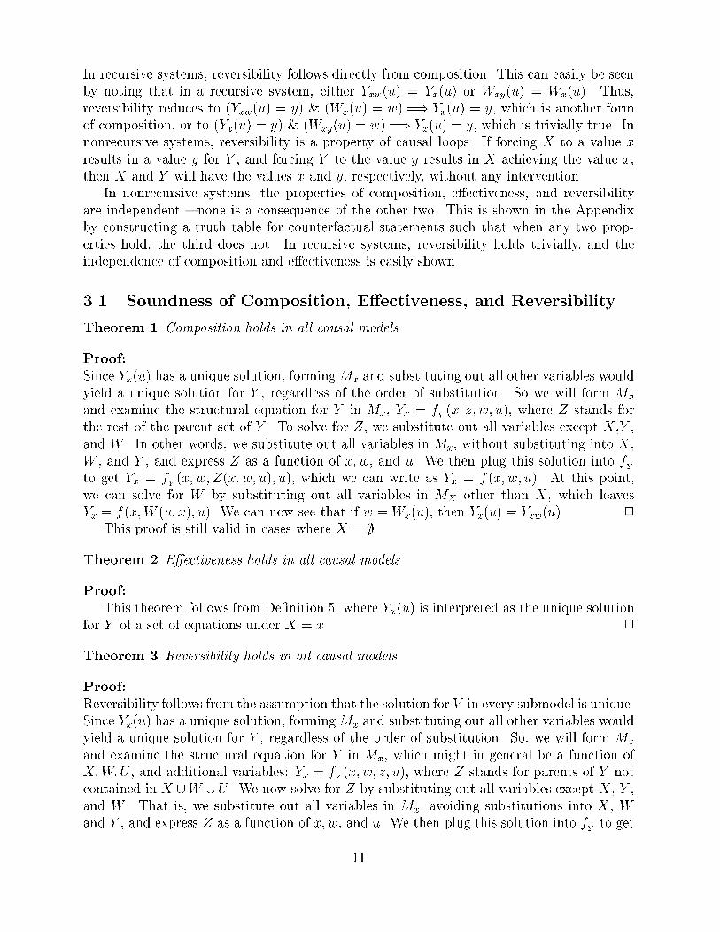
In recursive systems, reversibility follows directly from composition. This can easily be seenby noting that in a recursive system, either Yxw(u) = Yx(u) or Wxy(u) = Wx(u). Thus,reversibility reduces to (Yxw(u) = y) & (Wx(u) = w) =) Yx(u) = y, which is another formof composition, or to (Yx(u) = y) & (Wxy(u) = w) =) Yx(u) = y, which is trivially true. Innonrecursive systems, reversibility is a property of causal loops. If forcing X to a value xresults in a value y for Y , and forcing Y to the value y results in X achieving the value x,then X and Y will have the values x and y, respectively, without any intervention.In nonrecursive systems, the properties of composition, e�ectiveness, and reversibilityare independent { none is a consequence of the other two. This is shown in the Appendixby constructing a truth table for counterfactual statements such that when any two prop-erties hold, the third does not. In recursive systems, reversibility holds trivially, and theindependence of composition and e�ectiveness is easily shown.3.1 Soundness of Composition, E�ectiveness, and ReversibilityTheorem 1 Composition holds in all causal models.Proof:Since Yx(u) has a unique solution, formingMx and substituting out all other variables wouldyield a unique solution for Y , regardless of the order of substitution. So we will form Mxand examine the structural equation for Y in Mx, Yx = fY (x; z; w; u), where Z stands forthe rest of the parent set of Y . To solve for Z, we substitute out all variables except X,Y ,and W . In other words, we substitute out all variables in Mx; without substituting into X,W , and Y , and express Z as a function of x; w; and u. We then plug this solution into fYto get Yx = fY (x; w; Z(x; w; u); u), which we can write as Yx = f(x; w; u). At this point,we can solve for W by substituting out all variables in MX other than X, which leavesYx = f(x;W (u; x); u). We can now see that if w =Wx(u), then Yx(u) = Yxw(u). 2This proof is still valid in cases where X = ;.Theorem 2 E�ectiveness holds in all causal models.Proof:This theorem follows from De�nition 5, where Yx(u) is interpreted as the unique solutionfor Y of a set of equations under X = x. 2Theorem 3 Reversibility holds in all causal models.Proof:Reversibility follows from the assumption that the solution for V in every submodel is unique.Since Yx(u) has a unique solution, formingMx and substituting out all other variables wouldyield a unique solution for Y , regardless of the order of substitution. So, we will form Mxand examine the structural equation for Y in Mx, which might in general be a function ofX;W;U , and additional variables: Yx = fY (x; w; z; u), where Z stands for parents of Y notcontained in X [W [U . We now solve for Z by substituting out all variables except X, Y ,and W . That is, we substitute out all variables in Mx; avoiding substitutions into X, Wand Y , and express Z as a function of x; w, and u. We then plug this solution into fY to get11

Yx = fY (x; w; Z(x; w; u); u), which we can write as Yx = f(x; w; u). We now consider whatwould happen if we solved for Y inMxw. Since we avoided substituting anything intoW whenwe solved for Y inMx, we will get the same result as before, namely, Yxw = f(x; w; u). In thesame way, we can show that Wx = g(x; y; u) and Wxy = g(x; y; u). So, solving for y = Yx(u),w = Wx(u) is the same as solving for y = f(x; w; u) and w = g(x; y; u), which is the same assolving for y = Yxw(u), w =Wxy(u). Thus, any solution y to y = Yxw(u); w = Wxy(u) wouldalso be a solution to y = Yx(u). 2Reversibility re ects memoryless behavior { the state of the system, V , tracks the stateof U , regardless of U 's history. A typical example of irreversibility is a system of two agentswho adhere to a `tit-for-tat' strategy (e.g., the prisoners' dilemma). Such a system has twostable solutions, cooperation and defection, under the same external conditions U , and thusit does not satisfy the reversibility condition; forcing either one of the agents to cooperateresults in the other agent's cooperation (Yw(u) = y;Wy(u) = w), yet knowing this outcomedoes not guarantee cooperation from the start (Y (u) = y;W (u) = w). Irreversibility, insuch systems, is a product of using a state description that is too coarse, one where all ofthe factors that determine the ultimate state of the system are not included in U . In atit-for-tat system, the state description should include factors such as the previous actionsof the players, and reversibility is restored once the missing factors are included.3.2 Completeness of Composition and E�ectivenessDe�nition 8 (causal ordering) A causal ordering X1 : : :Xn of a set of variables is an or-dering such that for any two variables X = Xi and Y = Xk, i < k, we have Xyz(u) = Xz(u),where Z is any set of variables not including X or Y .Clearly, for every recursive model we can �nd an ordering that satis�es the condition ofDe�nition 8. In fact, every ordering consistent with the arrows of the causal graph G(M)will satisfy this condition. A system in which the variables are indexed along a speci�c causalordering will be called a causally ordered system.Theorem 4 Composition, together with e�ectiveness, are complete for causally ordered sys-tems, relative to conjunctions of counterfactual statements.A formal proof of completeness requires the explication of two properties, de�nitenessand uniqueness,7 which are implied by the de�nition of causal models (De�nition 1).Property 4 (de�niteness) For any variable X and set of variables Y ,9x 2 X s:t: Xy(u) = x (20)Property 5 (uniqueness) For every variable X and set of variables Y ,Xy(u) = x&Xy(u) = x0 =) x = x0 (21)7These two properties, de�niteness and uniqueness, were kept implicit in the completeness proof originallyreported in [Galles and Pearl, 1997a]; the bene�t to explicating them formally was brought to our attentionby [Halpern, 1998]. 12

De�nition 9 (statement) By a counterfactual statement, or statement for short, we denotea sentence of the form Yx(u) = y for a speci�c variable Y 2 V , a speci�c realization x of aset of variables X � V , and a speci�c u in the domain of U .De�nition 10 (semantic entailment) Given a set S of counterfactual statements, let MSbe the set of models of S, namely, the set fm1; : : : ; mng of all causal models such that allstatements in S hold for each mi. A counterfactual statement � is semantically entailed byS, written S j= �, if � holds in each mi 2MS.De�nition 11 (syntactic entailment) Given a set A of axioms, a set of counterfactual state-ments S syntactically entails a counterfactual statement �, written S `A �, if � can bederived from S using repeated applications of axioms from A together with the rules of logic.Denote by CO the set of n(n � 1)=2 statements Xyz(u) = Xz(u)8X; Y 2 V such thatX precedes Y in the causal ordering. De�ne AC to be the set fcomposition, e�ectiveness,de�niteness, uniqueness, COg. We want to show that all statements that are semanticallyentailed by S are also syntactically entailed by S, namely, thatS j= � =) S `AC �[Note that] the axiom of de�niteness require the use of disjunction, which is not part of asimple counterfactual statement as speci�ed in De�nition 9. Thus, [by limiting our targetsentences to conjunctions of counterfactual statements (De�nition 9), the language relativewhich we need to establish completeness is weaker than the one used for expressing axiomsAC .]To establish completeness, it is enough to show that every set of statements S thatis consistent with AC has a model. To see that this condition is su�cient to prove thecompleteness of AC , assume that there is some set S and statement p : Xz(u) = x such thatin every model consistent with S, p holds, and p is not derivable from S using AC . Since p isnot derivable from S, there must be some other statement p0 : Xz(u) = x0; x 6= x0, such thatS [ fp0g is consistent with AC . Since in every model consistent with S, Xz(u) = x holds, nomodel is consistent with S [ fp0g. Thus, if AC is not complete, then there must exist someset S 0 that is consistent with AC , and has no model. Looking at the contrapositive, if everyset of statements S that is consistent with AC has a model, then AC is complete.We now show that for any set of statements S, if S is consistent under AC then S hasa model. We will use the concept of a maximally consistent set, which is a standard tech-nique used to prove completeness in modal logic [Fagin et al., 1995]. Consider a maximallyconsistent set S�. That is, a superset of S that is consistent with AC such that any supersetof S� is not consistent with AC . We will show that there is a causal modelM which satis�esevery statement in S�, and thus satis�es every statement in S.8Proof (by induction): We prove that, for any maximally consistent set S�, there existsa causal model M which satis�es every statement in S�, by induction on the number ofvariables jV j in S�.8We thank Joseph Halpern for calling our attention to this technique which simpli�es appreciably thecompleteness proof originally reported in [Galles and Pearl, 1997a]. Halpern (1997) further shows that com-position and e�ectiveness are complete in recursive models for which the causal order is not speci�ed and,furthermore, the target language can be extended to disjunctions and negation of counterfactual statements.13

Base Case:If jV j = 1, then the statements X(u) in S� determine the function for X, and e�ectivenessensures that Xx(u) = x for all x 2 X.Inductive Case:Consider the variables V that are in S�. Let Y 2 V be the last element in the causal ordering.Consider the set S 0�, which is S� with all statements of the form Yz(u) = y and Xyz(u) = xremoved. By the inductive hypothesis, there is a model M 0 such that every element of S 0� issatis�ed.We now extend M 0 to M , such that every element in S� is satis�ed in M . For eachvariable X 2 M 0 and each value y of Y , fXM(x1; : : : ; xk; y; u) = fXM 0(x1; : : : ; xk; u). Wede�ne fY as follows: for each statement (Yz(u) = y) 2 S� such that jZj = jV j � 1 andY 62 Z, fY (z; u) = y. De�niteness ensures that fY will be completely determined.Since M 0 satis�ed all elements of S 0�, and given the causal ordering such that Xyz(u) =Xz(u) for all Xyz(u); Xz(u) in S�, M satis�es all statements of the form form Xz(u) in S�.We now show that M satis�es every element of S� of the form Yz(u) = y. We show thisby induction on the size of jV j � jZj.Base Cases:(i) Y 2 Z. By e�ectiveness, Yz(u) = y is in M .(ii) jV j � jZj = 1. By construction of fY , Yz(u) = y =) Y = y is in Mz.Inductive Case:jV j � jZj = k. Consider Yzx(u) = y0, where x = Xz(u). Above, we proved that Xz(u) issatis�ed in M , and by the inductive hypothesis, Yzx(u) = y0 is satis�ed in M . Thus, bycomposition, Yz(u) = y0 is satis�ed in M and, also by composition, y = y0. Thus, Yz(u) = yis satis�ed in M . 24 Comparison of Causal Models with Lewis's Closest-World FormalismWe now show that for recursive systems, composition and e�ectiveness are sound and com-plete within Lewis's closest-world framework [Lewis, 1973b]. We begin by providing a versionof Lewis's logic for counterfactual sentences (from [Lewis, 1981]).Rules(1) If A and A=)B are theorems, so is B.(2) If (B1 & : : :) =) C is a theorem, so is ((A2!B1) : : :) =) (A2! C).Axioms(1) All truth-functional tautologies.(2) A2! A.(3) (A2!B) & (B 2! A) =) (A2! C) � (B 2! C).(4) ((A _B) 2! A) _ ((A _ B)2!B) _ (((A _ B)2! C) � (A 2! C) & (B 2! C)).(5) A2! B =) A=)B.(6) A&B =) A 2!B. 14

The statement A 2! B stands for \In all closest worlds where A holds, B holds aswell." Lewis does not put any restrictions on the distance measured, except for the obviousrequirement that world w be no further from itself than any other world w0 6= w. In essence,causal models de�ne an obvious distance measure among worlds, d(w;w0), given by theminimal number of local interventions needed for transforming w into w0. As such, all ofLewis's axioms are true for causal models and follow from e�ectiveness, composition, and(for nonrecursive systems) reversibility.To relate Lewis's axioms to those of causal models, we must translate his syntax. Wewill equate Lewis's world with an instantiation of all the variables, including those in U ,in a causal model. Values of subsets of variables in causal models will stand for Lewis'spropositions, (e.g., A and B in the statements above). Thus, in a causal model, the meaningof the Lewis statement A 2! B is \If we force a set of variables to have the values A, asecond set of variables will have the values B." Let A stand for a set of values x1; : : : ; xnof the variables X1; : : : ; Xn, and let B stand for a set of values y1; : : : ; ym of the variablesY1; : : : ; Ym. Then A2!B � Y1x1:::xn(u) = y1 &Y2x1:::xn(u) = y2 &: : :Ymx1:::xn(u) = yn & (22)Conversely, we need to translate causal statements such as Yx(u) = y into Lewis's no-tation. Let A stand for the proposition X = x, and B stand for the proposition Y = y.Then Yx(u) = y � A2!B (23)We can now examine each of Lewis's axioms in turn.(1) This axiom is trivially true.(2) This axiom is the same as e�ectiveness: if we force a set of variables X to have thevalue x, then the resulting value of X is x. That is, Xx(u) = x.(3) This axiom is a weaker form of reversibility, which is relevant only for nonrecursivecausal models.(4) Because actions in are restricted to conjunctions of literals, this axiom is irrelevant.(5) This axiom follows directly from composition.(6) This axiom follows directly from composition.Likewise, composition and e�ectiveness follow from Lewis's axioms. Composition is aconsequence of axiom (5) and rule (1) in Lewis's formalism, while e�ectiveness is the sameas Lewis's axiom (2).In sum, for recursive models, the causal model framework does not add any restrictionsto counterfactual statements beyond those imposed by Lewis's framework; the very generalsystem of closest worlds is su�cient for recursive systems. When we consider nonrecursivesystems, however, we see that reversibility is not enforced by Lewis's framework. Lewis's15

axiom (3) is similar to, but not as strong as reversibility: that is, Y = y may hold in allclosest w-worlds,W = w may hold in all closest y-worlds, and Y = y still may not hold in theactual world. Nonetheless, we can safely conclude that in adopting the causal interpretationof counterfactuals, together with the representational and algorithmic machinery of modi�-able structural equation models, we are not introducing any restrictions on the structure ofcounterfactual statements in recursive systems.5 Applying Counterfactual Derivation: ExampleConsider the century-old debate over the e�ect of smoking on the incidence of lung cancer.According to many, the tobacco industry has managed to block anti-smoking legislationby arguing that the observed correlation between smoking (X) and lung cancer (Y) couldbe explained by some sort of carcinogenic genotype (U1) that involves inborn craving fornicotine.9 However, according to the Surgeon General's report of 1964, there is a causal linkbetween smoking and lung cancer that is mediated by the accumulation of tar (Z) depositedin a person's lungs. The two claims are combined in the graph of Figure 3, which representscausal models having the following structure:V = fX (Smoking), Y (Lung Cancer), Z (Tar in Lungs)gU = fU1; U2g; U1 k U2x = f1(u1)z = f2(x; u2)y = f3(z; u1)The graphical model embodies several assumptions. The missing link between X andY represents the assumption that the e�ect of smoking cigarettes (X) on the production oflung cancer (Y ) is entirely mediated through tar deposits in the lungs. To justify the missinglink between U1 and U2, we must assume that even if a genotype (U1) is aggravating theproduction of lung cancer, it nevertheless has no e�ect on the amount of tar in the lungsexcept indirectly, through cigarette smoking.To demonstrate how counterfactual analysis can help assess the degree to which cigarettesmoking increases (or decreases) lung cancer risk, imagine a study in which the three vari-ables, X; Y; and Z, were measured simultaneously on a large, randomly selected sample fromthe population. From such data, we wish to assess the risk of lung cancer (for a randomlychosen person in the population) under two hypothetical policies: smoking (X = 1) andrefraining from smoking (X = 0). In other words, we wish to derive an expression for theprobability of Y = y under the action do(X = x); P (Y = yjdo(x)) = P (Yx = y), based onthe joint distribution P (x; y; z) and the assumptions embodied in the graphical model.In [Pearl, 1995a] this problem was solved by a graphical method, using a set of ax-ioms which, when certain conditions hold in the graph, transform expressions of the formP (yjz; do(x)) into other expressions of this type, so as to eliminate the do(�) operator. Herewe show how the counterfactual expression P (Yx = y) can be reduced to ordinary proba-bilistic expression (involving no counterfactuals) by purely symbolic machinery, using onlyprobability calculus and two rules of inference: e�ectiveness and composition. To this end,9For an excellent historical account of this debate, see [Spirtes et al., 1993, pp. 291{302].16

we �rst need to translate the assumptions embodied in the graphical model into the lan-guage of counterfactuals. In [Pearl, 1995a, p. 704] it is shown that the translation can beaccomplished systematically, using two simple rules:Rule 1 Exclusion restrictions. For every variable Y having parents PAY , and for every set ofvariables Z disjoint of PAY , we haveYpaY (u) = YpaY z(u) (24)Rule 2 Independence restrictions. If Z1; : : : ; Zk is any set of nodes in V not connected to Yvia a path containing only U variables, we haveYpaY k fZ1paZ1 ; : : : ; ZkpaZk g (25)Rule 1 re ects the insensitivity of Y to any manipulation, once its direct causes PAY areheld constant; it follows from the identity vi = fi(pai; u) in De�nition 1. Rule 2 interpretsindependencies among U variables as independencies between the counterfactuals of thecorresponding V variables, with their parents held �xed. Indeed, the statistics of YpaY isgoverned by the equation Y = fY (paY ; uY ), therefore, once we hold PAY �xed the residualvariations of Y are governed solely by the variations in UY .U 2

U 1

X Z Y

Smoking Tar inLungs

Cancer

Figure 3: Causal graph illustrating the e�ect of smoking on lung cancer.Applying these two rules, we see that the causal graph encodes the following assumptions:Zx(u) = Zyx(u) (26)Xy(u) = Xzy(u) = Xz(u) = X(u) (27)Yz(u) = Yzx(u) (28)Zx k fYz; Xg (29)Eqs. (26-28) follow from the exclusion restrictions of Eq. (24), using:PAX = f;g; PAY = fZg and PAZ = fXg:17

Eq. (26), for instance, represents the absence of a causal link from Y to Z, while Eq. (27)represents the absence of a causal link from Z or Y to X. In contrast, Eq. (29) follows fromthe independence restriction of Eq. (25), since the lack of a connection between (i.e., theindependence of) U1 and U2 rules out any path between Z and fX; Y g that contains only Uvariables.We now use these assumptions, and the properties of composition and e�ectiveness, tocompute various tasks:Task 1 Compute P (Zx = z), i.e., the causal e�ect of smoking on tar.P (Zx = z) = P (Zx = zjx) from Eq. (29)= P (Z = zjx) by composition= P (zjx) (30)Task 2 Compute P (Yz = y), i.e., the causal e�ect of tar on cancer.P (Yz = y) = Xx P (Yz = yjx)P (x) (31)and since Eq. (29) implies Yz k ZxjX, we can writeP (Yz = yjx) = P (Yz = yjx; Zx = z) from Eq. (29)= P (Yz = yjx; z) by composition= P (yjx; z) by composition (32)Substituting Eq. (32) in Eq. (31) givesP (Yz = y) =Xx P (yjx; z)P (x) (33)Task 3 Compute P (Yx = y), i.e., the causal e�ect of smoking on cancer.For any variable Z,Yx(u) = Yxz(u); if Zx(u) = z by compositionSince Yxz(u) = Yz(u) (from Eq. (28)),Yx(u) = Yxzx(u) = Yz(u) where zx = Zx(u) (34)Thus, P (Yx = y) = P (Yzx = y) from Eq. (34)= Pz P (Yzx = yjZx = z)P (Zx = z)= Pz P (Yz = yjZx = z)P (Zx = z) by composition= Pz P (Yz = y)P (Zx = z) from Eq. (29) (35)18

P (Yx = y) and P (Zx = z) were computed in Eq. (30) and Eq. (33). Substituting givesus P (Yx = y) =Xz P (zjx)Xx0 P (yjz; x0)P (x0) (36)The right hand side of Eq. (36) can be computed from P (x; y; z) and coincides withthe \front-door" formula derived in [Pearl, 1995a].In general, a counterfactual quantity such as P (Yx = y) that can be reduced to expressionsinvolving probabilities of observed variables is called identi�able [Fisher, 1966; Pearl, 1997b].Our completeness result implies that any identi�able counterfactual quantity can be reducedto the correct expression by repeated application of composition and e�ectiveness.6 Conclusions and DiscussionThe completeness of composition and e�ectiveness in recursive causal models has two majorimplications. First, it shows that in systems with no feedback, the causal interpretationof counterfactuals adds no restrictions beyond those of Lewis's closest-world interpretation.Thus, the unstructured closest-worlds framework embodies all of the causal restrictions oncounterfactuals that are not embodied already by the requirement of recursiveness. In non-recursive systems, however, there is a di�erence between the two formalisms; the causalreading of counterfactuals imposes the additional restriction of reversibility.Second, the completeness result assures us that a deduction of counterfactual relation-ships in recursive models may safely be attempted with two axioms only, that is, all truthsderivable by structural equation semantics are also derivable using e�ectiveness and compo-sition. This establishes, in essence, the formal equivalence of structural equation modeling,popular in economics and the social sciences [Goldberger, 1992], and the potential-responseframework, as used in statistics [Rubin, 1974; Holland, 1986; Robins, 1986].10 In nonrecur-sive models, however, this is not necessarily the case. Attempts to evaluate counterfactualstatements using only composition and e�ectiveness may fail to certify some statements thatare true in all causal models but whose validity can only be recognized through the use ofreversibility.11The structural-counterfactual equivalence established in this paper does not in any waydiminish the usefulness of structural equations and graphs in causal analysis. Graphs andequations are indispensable tools for expressing the assumptions that make up a causalmodel. Such assumptions must rest on prior experiential knowledge, which, as suggestedby ample evidence, is encoded in the human mind in terms of interconnected assemblies ofautonomous mechanisms from which we draw inferences about actions, changes, and theirrami�cations. These mechanisms are thus the building blocks from which judgments about10This equivalence was anticipated in Holland (1988), Pratt and Schlai�er (1988), Pearl (1995), and Robins(1995). Note, though, that the equation-deletion part of our model (De�nition 2) is not made explicit in thestandard literature on structural equation modeling.11Joseph Halpern (1997) has recently shown that composition, reversibility, e�ectiveness, and de�nitenessare complete in recursive as well as nonrecursive models, as long as the uniqueness assumption holds. Healso characterized systems in which uniqueness does not hold, using axioms of more elaborate syntax.19

counterfactuals are derived. Structural equations ffig and their graphical abstraction G(M)provide faithful mapping for these mechanisms and constitute, therefore, the most naturallanguage for articulating or verifying causal assumptions. Thus, graphical speci�cation ofassumptions, followed by translation into counterfactual notation and then by symbolicderivation, as exempli�ed in Section 5, should yield a more e�ective method of analysis thana method that insists on expressing assumptions directly as counterfactuals. Indeed, anassumption such as the one expressed in Eq. (29) is not easily comprehended by even skilledinvestigators. In contrast, its structural image U1 k U2 evokes an immediate process-basedinterpretation.Graphs may also assist symbolic proof procedures [Galles and Pearl, 1997b] by display-ing independence relations (among counterfactuals as well as measured variables) that arenot easily derived symbolically [Balke and Pearl, 1994]. For example, it is not straightfor-ward to show that the assumptions of Eqs. (26)-(29) imply the conditional independence(Yz k ZxjfZ;Xg) but do not imply the conditional independence (Yz k ZxjZ). Suchimplications can be easily tested in the graph of Figure 3 or in the dual-graph method of[Balke and Pearl, 1994].But perhaps the most compelling reason for molding causal assumptions in the languageof graph is that such assumptions are needed before the data are gathered, at a stage whenthe model's parameters are still \free," that is, still to be determined from the data. Theusual temptation is to mold those assumptions in the language of statistical independence,which carries an aura of testability, hence of scienti�c legitimacy. However, conditions ofstatistical independence, regardless of whether they relate to V variables, U variables, orcounterfactuals, are generally sensitive to the values of the model's parameters, which are notavailable at the modeling phase. The substantive knowledge available at the modeling phasecannot support such assumptions unless they are stable, that is, insensitive to the valuesof the parameters involved [Pearl, 1998b]. The implications of graphical models, which restsolely on the interconnections among mechanisms, satisfy this stability requirement and cantherefore be ascertained from generic substantive knowledge, before data are collected. Forexample, the assertion (X k Y jZ; U1), which is implied by the graph of Figure 3, remainsvalid for any substitution of functions in ffig and for any assignment of prior probabilitiesto U1 and U2.These considerations apply not only to the formulation of causal assumptions but alsoto the language in which causal concepts are de�ned and communicated. Many concepts inthe social and medical sciences are de�ned in terms of relationships among unobserved Uvariables, also called errors or disturbance terms. For example, key econometric notions suchas exogeneity and instrumental variables have traditionally been de�ned in terms of absenceof correlation between certain observed variables and certain error terms in the equations thatgovern response variables. Naturally, such de�nitions attract criticism from strict empiricists,who regard unobservables as metaphysical or de�nitional [Richard, 1980; Engle et al., 1983;Holland, 1988], and from counterfactual analysts, who regard the use of equations as anunwarranted commitment to a particular functional form [Angrist et al., 1996].The analyses of this paper shed new light on this controversy by explicating the op-erational meaning of the \so-called disturbance terms" [Richard, 1980] and by clarifyingthe relationships among error-based, counterfactual, and graphical de�nitions. These threemodes of description form a simple hierarchy. Since graph separation implies independence,20

but independence does not imply graph separation [Pearl, 1988], de�nitions based on graphseparation should imply those based on error-term independence. Likewise, since for anytwo variables X and Y the independence relation UX k UY implies the counterfactual in-dependence XpaX k YpaY (but not the other way around), it follows that de�nitions basedon error independence should imply those based on counterfactual independence. Overall,we have the hierarchy:Graphical criteria ) Error-based criteria ) Counterfactual criteriaThe econometric notion of exogeneity may serve to illustrate this hierarchy. The prag-matic de�nition of exogeneity is best formulated in counterfactual or interventional terms,and reads:Counterfactual exogeneity: X is exogenous relative to Y i� the e�ect of X on Y isidentical to the conditional probability of Y given X, namely, ifP (Yx = y) = P (yjx) (37)or, equivalently, P (Y = yjdo(x)) = P (yjx) (38)which, in turns, is equivalent to the independence condition Yx k X, named \ignorability"in [Rosenbaum and Rubin, 1983].This de�nition is pragmatic, in that it highlights the reasons economists should be con-cerned with exogeneity by explicating the policy-analytic bene�ts of discovering that a vari-able is exogenous. However, this de�nition fails to guide an investigator into verifying, fromsubstantive knowledge of the domain, whether the condition above holds in any given sys-tem, especially when many equations are involved. To facilitate such judgments, economists[e.g., Koopmans, 1950] have adopted the error-based de�nition:Error-based exogeneity: X is exogenous in M relative to Y if X is independent of allerror terms that have an in uence on Y that is not mediated by X.12This de�nition is more transparent to human judgment because the reference to errorterms tends to focus attention on speci�c factors, potentially a�ecting Y , with which ascientist is familiar. Still, to judge whether such factors are statistically independent is adi�cult mental task unless the independencies considered are dictated by topological con-siderations, which assures their stability. Indeed, the most popular conception of exogeneityis encapsulated in the notion of \common cause," formally:Graphical exogeneity: X is exogenous relative to Y if X and Y have no common ancestorin G(M).13It is not hard to show that the graphical condition implies the error-based condition,which, in turns, implies the counterfactual (or pragmatic) condition of Eq. (38). The latterimplication immediately rules out any contention that the error terms are metaphysical or12Independence relative to all errors is sometimes required in the literature (e.g., Dhrymes, 1970, p. 169),but this is obviously too strong.13The augmented graphG(M) should be used in this test, where a latent common parent is added for everypair of dependent errors. This de�nition paraphrases the \back-door criterion" [Pearl, 1995a] in the specialcase of no covariates. The incorporation of observed covariates is straightforward in all three de�nitions.21

de�nitional, as suggested by Hendry (1995, p. 62) and Holland (1988, p. 460). The equality inEq. (38), and hence its error-independence implicant, is clearly within the realm of empiricalveri�cation, albeit requiring controlled experiments. From a narrow empiricist viewpoint,the meaning of an error term uY is de�ned through the equation YpaY = fY (paY ; uY ), whichstates that the variable UY is merely a convenient device for encoding variations in thefunctional mapping from PAY to Y . The statistics of these variations are observable whenpaY is held �xed. From a broader perspective, however, the error terms can be viewed as(summaries of) a highly structured background knowledge, whose empirical basis may welllie outside the boundaries of speci�c study at hand [Pearl, 1998a].A three-level hierarchy similarly characterizes the notion of instrumental variables [Bow-den and Turkington, 1984; Pearl, 1995b]. The traditional de�nition quali�es a variable Zas instrument (relative the pair (X; Y )) if (i) Z is independent of all terms in the equationfor Y (excluding X and variables a�ected by X) and (ii) Z is not independent of X. Thecounterfactual de�nition replaces the former condition with (i0) Z is independent of Yx, whilethe corresponding graphical condition reads (i00) every path connecting Z and Y must passthrough X, unless it contains arrows pointing head-to-head.Note that, in both examples, the graphical de�nitions are insensitive to the value ofthe model's parameters and can therefore be ascertained using our general, qualitative un-derstanding of how mechanisms and processes are tied together. It is for this reason thatgraphical vocabulary guides and expresses so well our intuition about exogeneity, instru-ments, confounding, and even (I speculate) more technical notions such as randomness andstatistical independence.AcknowledgmentThis investigation has bene�ted signi�cantly from the input of Joseph Halpern and fromdiscussions with John Aldrich, Phil Dawid, David Freedman, Arthur Goldberger, SanderGreenland, Paul Holland, Guido Imbens, Ed Leamer, Charles Manski, Jamie Robins, DonRubin, and Glenn Shafer. The research was partially supported by AFOSR, NSF, Northrop,and Rockwell.Appendix AIndependence of Composition, E�ectiveness, and ReversibilityWe show that reversibility, composition, and e�ectiveness are independent by creating atable of counterfactual statements such that two of the properties hold, but the third doesnot. We will consider a small model, one with only two binary variables X and Y , and asingle value for U .22

A.1 Composition and E�ectiveness, not ReversibilityX = 0 Y = 0XX=0 = 0 YX=0 = 0 XX=0;Y=0 = 0 YX=0;Y=0 = 0XX=1 = 1 YX=1 = 1 XX=0;Y=1 = 0 YX=0;Y=1 = 1XY=0 = 0 YY=0 = 0 XX=1;Y=0 = 1 YX=1;Y=0 = 0XY=1 = 1 YY=1 = 1 XX=1;Y=1 = 1 YX=1;Y=1 = 1A.2 E�ectiveness and Reversibility, not CompositionX = 0 Y = 1XX=0 = 0 YX=0 = 1 XX=0;Y=0 = 0 YX=0;Y=0 = 0XX=1 = 1 YX=1 = 0 XX=0;Y=1 = 0 YX=0;Y=1 = 1XY=0 = 0 YY=0 = 0 XX=1;Y=0 = 1 YX=1;Y=0 = 0XY=1 = 1 YY=1 = 1 XX=1;Y=1 = 1 YX=1;Y=1 = 1A.3 Composition and Reversibility, not E�ectivenessX = 0 Y = 1XX=0 = 0 YX=0 = 1 XX=0;Y=0 = 0 YX=0;Y=0 = 1XX=1 = 0 YX=1 = 1 XX=0;Y=1 = 0 YX=0;Y=1 = 1XY=0 = 0 YY=0 = 1 XX=1;Y=0 = 0 YX=1;Y=0 = 1XY=1 = 0 YY=1 = 1 XX=1;Y=1 = 0 YX=1;Y=1 = 1

23

References[Angrist et al., 1996] J.D. Angrist, G.W. Imbens, and Rubin D.B. Identi�cation of causale�ects using instrumental variables (with comments). Journal of the American StatisticalAssociation, 91(434):444{472, June 1996.[Balke and Pearl, 1994] A. Balke and J. Pearl. Counterfactual probabilities: Computationmethods, bounds, and applications. In R.L. de Mantaras and D. Poole, editors, Proceed-ings of the Tenth Conference on Uncertainty in Arti�cial Intelligence, pages 11{18, SanFrancisco, 1994. Morgan Kaufmann.[Balke and Pearl, 1995] A. Balke and J. Pearl. Counterfactuals and policy analysis in struc-tural models. In P. Besnard and S. Hanks, editors, Proceedings of the Eleventh Conferenceon Uncertainty in Arti�cial Intelligence, pages 11{18, San Francisco, 1995. Morgan Kauf-mann.[Bowden and Turkington, 1984] R.J. Bowden and D.A. Turkington. Instrumental Variables.Cambridge University Press, Cambridge, MA, 1984.[Dawid, 1997] A.P. Dawid. Causal inference without counterfactuals. Technical Report,Department of Statistical Science, University College London, UK, 1997.[Dhrymes, 1970] P.J. Dhrymes. Econometrics. Springer-Verlag, New York, 1970.[Engle et al., 1983] R.F. Engle, D.F. Hendry, and J.F. Richard. Exogeneity. Econometrical,51(2):277{304, March 1983.[Fagin et al., 1995] R. Fagin, J.Y. Halpern, Y. Moses, and M.Y. Vardi. Reasoning AboutKnowledge. MIT Press, Cambridge, MA, 1995.[Fisher, 1966] F.M. Fisher. The Identi�cation Problem in Econometrics. McGraw-Hill, NewYork, 1966.[Fisher, 1970] F.M. Fisher. A correspondence principle for simultaneous equation models.Econometrica, 38:73{92, 1970.[Galles and Pearl, 1997a] D. Galles and J. Pearl. An axiomatic characterization of causalcounterfactuals. Technical Report R-250-L, Computer Science Department, Universityof California, Los Angeles, March 1997. Prepared for Foundations of Science, KluwerAcademic Publishers.[Galles and Pearl, 1997b] D. Galles and J. Pearl. Axioms of causal relevance. Arti�cialIntelligence, 97(1-2):9{43, 1997.[Gibbard and Harper, 1981] A. Gibbard and L. Harper. Counterfactuals and two kinds ofexpected utility. In W.L. Harper, R. Stalnaker, and G. Pearce, editors, Ifs. D. Reidel,Dordrecht: Holland, 1981. 24

[Ginsberg and Smith, 1987] M.L. Ginsberg and D.E. Smith. Reasoning about action I: Apossible worlds approach. In Frank M. Brown, editor, The Frame Problem in Arti�cialIntelligence, pages 233{258. Morgan Kaufmann, Los Altos, CA, 1987.[Goldberger, 1992] Arthur S. Goldberger. Models of substance [comment on N. Wermuth,\On block-recursive linear regression equations"]. Brazilian Journal of Probability andStatistics, 6:1{56, 1992.[Halpern, 1998] J. Halpern. Axiomatizing causal reasoning. Unpublished report, CornellUniversity, February, 1998.[Heckerman and Shachter, 1995] D. Heckerman and R. Shachter. A de�nition and graphi-cal representation of causality. In P. Besnard and S. Hanks, editors, Proceedings of theEleventh Conference on Uncertainty in Arti�cial Intelligence, pages 262{273, San Fran-cisco, 1995. Morgan Kaufmann.[Hendry, 1995] David F. Hendry. Dynamic Econometrics. Oxford University Press, NewYork, 1995.[Holland, 1986] P. W. Holland. Statistics and causal inference (with discussion). Journal ofthe American Statistical Association, 81(396):945{970, 1986.[Holland, 1988] P.W. Holland. Causal inference, path analysis, and recursive structuralequations models. In C. Clogg, editor, Sociological Methodology, pages 449{484. AmericanSociological Association, Washington, D.C., 1988.[Katsuno and Mendelzon, 1991] H. Katsuno and A.O. Mendelzon. On the di�erence betweenupdating a knowledge base and revising it. In Principles of Knowledge Representation andReasoning: Proceedings of the Second International Conference, pages 387{394, Boston,MA, 1991.[Koopmans, 1950] T.C. Koopmans. When is an equation system complete for statisticalpurposes? In T.C. Koopmans, editor, Statistical Inference in Dynamic Economic Models,Cowles Commission, Monograph 10. Wiley, New York, 1950. Reprinted in D.F. Hendryand M.S. Morgan (Eds.), The Foundations of Econometric Analysis, Cambridge UniversityPress, 527{537, 1995.[Leamer, 1985] E. Leamer. Vector autoregression for causal inference? Carnegie-RochesterConference Series on Public Policy, 22:255{304, 1985.[Lewis, 1973a] D. Lewis. Causation. Journal of Philosophy, 70:556{567, 1973.[Lewis, 1973b] D. Lewis. Counterfactuals. Harvard University Press, Cambridge, MA, 1973.[Lewis, 1981] D. Lewis. Counterfactuals and comparative possibility. In W.L. Harper,R. Stalnaker, and G. Pearce, editors, Ifs. D. Reidel, Dordrecht, Holland, 1981.[Manski, 1990] C.F. Manski. Nonparametric bounds on treatment e�ects. American Eco-nomic Review, Papers and Proceedings, 80:319{323, 1990.25

[Meditch, 1969] J.S. Meditch. Stochastic Optimal Linear Estimation and Control. McGraw-Hill, New York, 1969.[Pearl, 1988] J. Pearl. Probabilistic Reasoning in Intelligent Systems. Morgan Kaufmann,San Mateo, CA, 1988. (Revised 2nd printing, 1992).[Pearl, 1994] J. Pearl. A probabilistic calculus of actions. In R.L. de Mantaras and D. Poole,editors, Proceedings of the Tenth Conference on Uncertainty in Arti�cial Intelligence,pages 454{462, San Francisco, 1994. Morgan Kaufmann.[Pearl, 1995a] J. Pearl. Causal diagrams for empirical research (with discussion). Biometrika,82(4):669{710, 1995.[Pearl, 1995b] J. Pearl. On the testability of causal models with latent and instrumentalvariables. In P. Besnard and S. Hanks, editors, Uncertainty in Arti�cial Intelligence 11,pages 435{443. Morgan Kaufmann, 1995.[Pearl, 1996] J. Pearl. Structural and probabilistic causality. Psychology of Learning andMotivation, 34:393{435, 1996.[Pearl, 1997a] J. Pearl. The new challenge: From a century of statistics to an age of causa-tion. Computing Science and Statistics, 29(2):415{423, 1997.[Pearl, 1997b] J. Pearl. On the identi�cation of nonparametric structural models. InM. Berkane, editor, Latent Variable Modeling with Application to Causality, pages 29{68. Springer-Verlag, 1997.[Pearl, 1998a] J. Pearl. Graphs, causality, and structural equation models. Technical ReportR-253, Department of Computer Science, University of California, Los Angeles, 1998. Toappear in Socioligical Methods and Research, Special Issue on Causality.[Pearl, 1998b] J. Pearl. Why there is no statistical test for confounding, why many thinkthere is, and why they are almost right. Technical Report R-256, Department of ComputerScience, University of California, Los Angeles, 1998.[Pratt and Schlaifer, 1988] J.W. Pratt and R. Schlaifer. On the interpretation and observa-tion of laws. Journal of Econometrics, 39:23{52, 1988.[Richard, 1980] J.F. Richard. Models with several regimes and charges in exogeneity. TheReview of Economic Studies, 47:1{20, 1980. from orion.[Robins, 1986] J. Robins. A new approach to causal inference in mortality studies with asustained exposure period { applications to control of the healthy workers survivor e�ect.Mathematical Modeling, 7:1393{512, 1986.[Robins, 1987] J. Robins. Addendum to \A new approach to causal inference in mortalitystudies with sustained exposure periods { application to control of the healthy workersurvivor e�ect". Computers and Mathematics, with Applications., 14:923{45, 1987.26

[Robins, 1995] J.M. Robins. Discussion of \Causal diagrams for empirical research" byJ. Pearl. Biometrika, 82(4):695{698, 1995.[Rosenbaum and Rubin, 1983] P. Rosenbaum and D. Rubin. The central role of propensityscore in observational studies for causal e�ects. Biometrika, 70:41{55, 1983.[Rubin, 1974] D.B. Rubin. Estimating causal e�ects of treatments in randomized and non-randomized studies. Journal of Educational Psychology, 66:688{701, 1974.[Simon and Rescher, 1966] H.A. Simon and N. Rescher. Cause and counterfactual. Philos-ophy and Science, 33:323{340, 1966.[Sobel, 1990] M.E. Sobel. E�ect analysis and causation in linear structural equation models.Psychometrika, 55:495{515, 1990.[Spirtes et al., 1993] P. Spirtes, C. Glymour, and R. Scheines. Causation, Prediction, andSearch. Springer-Verlag, New York, 1993.[Strotz and Wold, 1960] R.H. Strotz and O.A. Wold. Recursive versus nonrecursive systems:An attempt at synthesis. Econometrica, 28:417{427, 1960.[Winslett, 1988] M. Winslett. Reasoning about action using a possible worlds approach. InProceedings of the Seventh American Association for Arti�cial Intelligence Conference,pages 89{93, 1988.

27