Embed Size (px)
Citation preview

AN OVERVIEW OF WAVELET BASED
MULTIRESOLUTION ANALYSES�
BJ�ORN JAWERTHyz AND WIM SWELDENSyx
Abstract. In this paper we present an overview of wavelet based multiresolution analyses.
First, we brie y discuss the continuous wavelet transform in its simplest form. Then, we give the
de�nition of a multiresolution analysis and show how wavelets �t into it. We take a closer look at
orthogonal, biorthogonal and semiorthogonal wavelets. The fast wavelet transform, wavelets on an
interval, multidimensional wavelets and wavelet packets are discussed. Several examples of wavelet
families are introduced and compared. Finally, the essentials of two major applications are outlined:
data compression and compression of linear operators.
Key words. wavelet, multiresolution analysis, compression
AMS subject classi�cations. 42-02, 42C10
Contents.
1. Introduction2. Notation3. A short history of wavelets4. The continuous wavelet transform5. Multiresolution analysis6. Orthogonal wavelets7. Biorthogonal wavelets8. Wavelets and polynomials9. The fast wavelet transform10. Examples of wavelets11. Wavelets on an interval12. Wavelet packets13. Multidimensional wavelets14. Applications
1. Introduction. Wavelets have generated a tremendous interest in both the-oretical and applied areas, especially over the past few years. The number of re-searchers, already large, continues to grow, so progress is being made at a rapid pace.In fact, advancements in the area are occurring at such a rate that the very meaningof \wavelet analysis" keeps changing to incorporate new ideas.
In a rapidly developing �eld, overview papers are particularly useful, and severalgood ones concerning wavelets are already available, such as [60, 83, 115, 122, 123,125]. Of these, [122] contains a brief introduction to multiresolution analysis, [60]describes wavelets from an approximation theory point of view, [83] discusses contin-uous and discrete wavelets, [125] focuses on the construction of wavelets, [115] looksat wavelets from a signal processing point of view and [123] compares wavelets withFourier techniques.
� Manuscript recieved by the editors ??, accepted for publication ??y Department of Mathematics, University of South Carolina, Columbia SC 29208z This author is partially supported by DARPA Grant AFOSR F49620-93-1-0083 and ONR Grant
N00014-90-J-1343.x Departement Computerwetenschappen, Katholieke Universiteit Leuven, Celestijnenlaan 200 A,
B 3001 Leuven, Belgium. This author is Research Assistant of the National Fund of Scienti�c
Research Belgium, and is partially supported by ONR Grant N00014-90-J-1343and the Experimental
Program to Stimulate Competitive Research (EPSCOR NSF Grant EHR-9108772).
1

2 BJORN JAWERTH AND WIM SWELDENS
Our paper di�ers from these in that it contains some more recent developmentsand that it focuses on the \multiresolution analysis" aspect of wavelets. The emphasison multiresolution analysis allows us to look at a number of di�erent constructionsof wavelets such as orthogonal, semiorthogonal, and biorthogonal wavelets. By ex-amining these constructions in a uni�ed setting, we are ideally positioned to makecomparisons between them. The recent developments contain wavelets on an interval,multidimensional wavelets, and wavelet packets.
We have selected an expository style and a level of rigor that we hope will presentthe ideas without obscuring them in too much detail. Instead of giving exact, detailedstatements in a \theorem-structured" way, we have opted for a more informal style.References are given throughout, pointing to more details when needed.
For example, this paper occasionally contains statements of the form \A is (es-sentially) equivalent with B". The interpretation that we have in mind is that, for\all practical purposes", A is equivalent to B. Strictly speaking, the equivalence mayonly hold under some extra technical conditions. Good examples are when a formulais guaranteed to be true only \almost everywhere" or in a \weak sense".
The style we have chosen is motivated by the intended audience: people witha more theoretical interest as well as those working in various applied areas. For areader in the �rst category this paper might provide some of the theory, and point tosome of the right references for further study. A reader in the second category coulduse the paper to make comparisons, and �nd connections to related material.
The paper is organized as follows. After a brief sketch of the history of waveletswe introduce the \continuous wavelet transform." The discussion of the continuouswavelet transform is mainly included for historical purposes and for comparison withthe multiresolution analysis wavelets. Next, we give the de�nitions of \multiresolu-tion analysis" and \scaling function" (Section 5), derive some basic properties andillustrate these with some examples. In this section we also give the basic de�nitionof \wavelet." Wavelets are then studied in more detail in the next sections. Section 6discusses orthogonal wavelets, while Section 7 treats biorthogonal wavelets, a gener-alization of the orthogonal ones, and semiorthogonal wavelets, a compromise betweenthe previous two. In the following section we study the connection between waveletsand polynomials, and show how this relates to the approximation properties of wave-let expansions. In Section 9 we show how a \fast wavelet transform" can be derivedfrom the multiresolution analysis properties. In the appendix, the reader can �nd apseudocode implementation of this algorithm. At this point, i.e. after the study of thebasic properties of multiresolution analysis, we are ready to single out some desirableproperties of wavelets. This is done in Section 10. We also give several examples ofwavelet families, such as Daubechies' and spline wavelets, and compare their prop-erties. The next three sections focus on more recent developments such as waveletson an interval, wavelet packets and multidimensional wavelets. These sections canbe read independently. Finally, in the last section (Section 14) we consider the basicideas associated with two important applications: data compression and analysis oflinear operators.
It goes without saying (almost) that this short overview is still highly incomplete.It is unfortunate that we were unable to cover many other important and interestingdevelopments in the area, some of which are more signi�cant than the ones we haveincluded. For example, we hardly mention the signi�cant volume of work done in thedirection of approximation theory, and the e�orts in the �eld of fractal functions andthe more applied areas are left out almost entirely. We apologize to the people whose

AN OVERVIEW OF WAVELET BASED MULTIRESOLUTION ANALYSES 3
results we were unable to discuss due to the constraints imposed by the overviewformat.
Finally, let us point out that, although wavelets are a relatively recent phe-nomenon, there are a number of useful sources of information about them. Firstof all, there are three new journals with an emphasis on wavelets: Applied Compu-tational Harmonic Analysis, Journal of Fourier Analysis, and Advances in Compu-tational Mathematics. Secondly, several journals have had special issues on wave-lets, such as Constructive Approximation, IEEE Transactions on Signal Process-ing, IEEE Transactions on Information Theory, International Journal of OpticalComputing, Journal of Mathematical Imaging and Vision, and Optical Engineer-ing. Also, an electronic information service exists on the Internet, the WaveletDigest, with the address [email protected]. Last but not least, severalbooks on the subject exist, monographs as well as edited volumes. The list includes[13, 20, 21, 43, 49, 74, 92, 96, 106, 108, 116, 119].
2. Notation. Most of the notation will be presented as we go along. The spaceof square integrable functions, L2(R), is de�ned as the space of Lebesgue measurablefunctions for which
kfk2 =Z +1
�1
jf(x)j2 dx <1:
The inner product of two functions f; g 2 L2(R) is given by
h f; g i =Z +1
�1
f(x) g(x)dx;
and the Fourier transform of a function f 2 L2(R) is de�ned as
bf(!) = Z +1
�1
f(x) e�i!x dx:
The Poisson summation formula is used in the following two forms,Xl
f(x� l) =Xk
bf(2k�) ei2k�x;and X
l
h f; g(� � l) i e�i!l =Xk
bf(! + k2�)bg(! + k2�):
If no bounds are indicated under a summation sign, 2 Z is understood.A countable set ffng of a Hilbert space is a Riesz basis if every element f of the
space can be written uniquely as f =P
n cn fn, and positive constants A and B existsuch that
A kfk2 6Xn
jcnj2 6 B kfk2:
3. A short history of wavelets. The history of wavelets could be the topic ofa separate paper. Let us give a short, subjective account.
Wavelet theory involves representing general functions in terms of simpler, �xedbuilding blocks at di�erent scales and positions. This has been found to be a useful
4 BJORN JAWERTH AND WIM SWELDENS
approach in several di�erent areas. For example, we have subband �ltering techniques,quadrature mirror �lters, pyramid schemes, etc., in signal and image processing, whilein mathematical physics similar ideas are studied as part of the theory of CoherentStates. Wavelet theory represents a useful synthesis of these di�erent approaches.
In abstract mathematics, it has been known for quite some time that techniquesbased on Fourier series and Fourier transforms are not quite adequate for many prob-lems and so-called Littlewood-Paley techniques often are e�ective substitutes. Thesetechniques were initially developed in the 30's to understand, among other things,summability properties of Fourier series and boundary behavior of analytic functions.In the 50's and 60's, these developed into powerful tools for studying other things,such as solutions of partial di�erential equations and integral equations. It was real-ized that they �t into Calder�on{Zygmund theory , an area of harmonic analysis thatis still very heavily researched.
One of the standard approaches, not only in Calder�on-Zygmund theory, but inanalysis in general, is to break up a complicated phenomenon into many simple piecesand study each of the pieces separately. In the 70's, sums of simple functions, calledatomic decompositions [35], were widely used, especially in Hardy space theory. Onemethod used to establish that a general function f has such a decomposition, is tostart with the \Calder�on formula": for a function f , one has that
f(x) =
Z +1
0
Z +1
�1
( t � f)(y) e t(x� y) dy dtt:
The � denotes convolution. Here t(x) = t�1 (x=t), and e t(x) is de�ned similarly,
for appropriate �xed functions and e . As we shall see below, this representa-tion is an example of a continuous wavelet transform. In mathematical physics theAslaksen-Klauder construction of the (ax+ b)-coherent states can be seen as anotherindependent derivation of the Calder�on formula [7, 91].
In the early 80's, Str�omberg discovered the �rst orthogonal wavelets [126]. Thiswas done in the context of trying to further understand Hardy spaces, as well as otherspaces used to measure the size and smoothness of functions. A discrete version ofthe Calder�on formula had also been used for similar purposes in [86] and long beforethis there were results by Haar [81], Franklin [70], Ciesielski [26], Peetre [112], andothers.
Independent from these developments in harmonic analysis, Alex Grossmann,Jean Morlet, and their coworkers studied the wavelet transform in its continuousform [78, 79, 80]. The theory of \frames" [51] provided a suitable general frameworkfor these investigations.
In the early to mid 80's, several groups, perhaps most notably the one associatedwith Yves Meyer and his collaborators, independently realized, with some excitement,that tools from Calder�on-Zygmund theory, in particular the Littlewood-Paley repre-sentations, had discrete analogs and could give a uni�ed view of many of the resultsin harmonic analysis. Also, one started to understand that these techniques couldbe e�ective substitutes for Fourier series in numerical applications. (The �rst namedauthor of this paper came to this understanding through the joint work with MikeFrazier [71, 72, 73].) As the emphasis shifted more towards the representations them-selves, and the building blocks involved, the name of the theory also shifted. AlexGrossmann and Jean Morlet suggested the word \wavelet" for the building blocks,and what earlier had been referred to as Littlewood-Paley theory, now started to becalled wavelet theory.

AN OVERVIEW OF WAVELET BASED MULTIRESOLUTION ANALYSES 5
Pierre-Gilles Lemari�e and Yves Meyer [97], independent of Str�omberg, constructednew orthogonal wavelet expansions. With the notion of multiresolution analysis, in-troduced by St�ephane Mallat and Yves Meyer, a systematic framework for under-standing these orthogonal expansions was developed [103, 104, 105]. It also providedthe connection with quadrature mirror �ltering. Soon, Ingrid Daubechies [47] gave aconstruction of wavelets, non-zero only on a �nite interval and with arbitrarily high,but �xed, regularity. This takes us up to a fairly recent time in the history of wavelettheory. Several people have made substantial contributions to the �eld over the pastfew years. Some of their work and the appropriate references will be discussed in thebody of the paper.
4. The continuous wavelet transform. Since we are going to be brief, letus start by pointing out that more detailed treatments of the continuous wavelettransform can be found in [20, 77, 78, 83]. As mentioned above, a wavelet expansionuses translations and dilations of one �xed function, the wavelet 2 L2(R). In thecase of the continuous wavelet transform, the translation and dilation parameters varycontinuously. In other words, the transform makes use of the functions
a;b(x) =1pjaj
�x� ba
�with a; b 2 R; a 6= 0:
These functions are scaled so that their L2(R) norms are independent of a. Thecontinuous wavelet transform of a function f 2 L2(R) is now de�ned by
W(a; b) = h f; a;b i :(1)
Using Parseval's identity, we can also write this as
2�W(a; b) = h bf; b a;b i ;(2)
where
b a;b(!) = apjaj
e�i!b b (a!):We assume now that the wavelet and its Fourier transform b are functions with
�nite centers �x and �! and �nite radii �x and �!. These quantities are de�ned by
�x =1
k k2
Z +1
�1
x j (x)j2 dx;
�2x =
1
k k2
Z +1
�1
(x� �x)2 j (x)j2 dx;
and similarly for �! and �!. The variable x usually represents either time or space;we shall settle for the �rst and refer to x as time. From (1) and (2), we see thatthe continuous wavelet transform at (a; b) picks up information about f , mostly fromthe time interval [b+ a�x� a�x; b+ a�x+ a�x] and from the frequency interval [(�! ��!)=a; (�! + �!)=a]. These two intervals determine a time-frequency window . Itswidth, height and position are governed by a and b. Its area is constant and given by4�x�!. The Heisenberg uncertainty principle says that this area has to be greaterthan 2. These time-frequency windows are also called Heisenberg boxes .

6 BJORN JAWERTH AND WIM SWELDENS
Suppose that the wavelet satis�es the admissibility condition
C =
Z +1
�1
j b (!)j2!
d! <1:
Then, the continuous wavelet transform W(a; b) is invertible on its range, and aninverse transform is given by the relation
f(x) =1
C
Z +1
�1
Z +1
�1
W(a; b) a;b(x)da db
a2:(3)
From the admissibility condition, we see that b (0) has to be 0, and, in particular, has to oscillate. This, together with the decay property, has given the name waveletor \small wave" (French: ondelette). This shows that the frequency localization ofthe wavelets is much better than pointed out above. In most cases �! is zero and thefrequency localization is really in a band [�!2=a;�!1=a][ [!1=a; !2=a], because b (0)vanishes. This can help to understand why a reconstruction formula of type (3) ispossible.
The transform is often represented graphically and plotted as two two-dimensionalimages with color or grey-scale value corresponding to the modulus and phase ofW(a; b). This representation has been used extensively in areas such as geophysics.
In applications, it is of interest to �nd inverse transforms that do not make useof W over the whole range of a and b. Transforms exist that only use positive valuesof a or even only discrete values for a. Furthermore, using the theory of frames it ispossible to study the case where only discrete values for a and b are used, see [83]for an excellent overview. The most common choice is to use a dyadic grid, i.e. tolet a = 2�j and b=a = l with j; l 2 Z [48, 73]. In general, the fewer values of a andb one wants to use, the more restrictive the condition on the wavelet becomes. Thecontinuous wavelet transform allows us to use a very general wavelet. At the otherextreme, we shall see that much more restrictive conditions hold for a wavelet used inmultiresolution analysis. This allows us, on the other hand, to prove powerful resultssuch as the construction of orthogonal bases.
The transform that only uses the dyadic values of a and b was originally calledthe discrete wavelet transform. At this moment, however, this term is ambiguous,since it is also used to denote the transform from the sequence of scaling functioncoe�cients of a function to its wavelet coe�cients (see Section 9).
The case when a, and b belong to more irregular sets have also been covered.Such irregular sampling results can be found in [14, 39, 68, 67].
The continuous wavelet transform is also used in singularity detection and char-acterization [71, 100]. A typical result in this direction is that if a function f is H�older(Lipschitz) continuous of order 0 < � < 1, so that jf(x + h) � f(x)j = O(h�), thenthe continuous wavelet transform has an asymptotic behavior like
W(a; b) = O(a�+1=2) for a! 0:
The converse is true as well. The advantage of this characterization compared to theFourier transform is that it does not only provide information about the kind of sin-gularity, but also about its location in time. There is a corresponding characterizationof H�older (Lipschitz) continuous functions of higher order � > 1; the wavelet mustthen have a number of vanishing moments greater than �, i.e.Z +1
�1
(x)xp dx = 0 for 0 6 p 6 � and p 2 Z:

AN OVERVIEW OF WAVELET BASED MULTIRESOLUTION ANALYSES 7
We note that the number of vanishing wavelet moments limits the order of smoothnessthat can be characterized.
Example. A classical example of a wavelet is the Mexican hat function,
(x) = (1� 2x2)e�x2
:
Being the second derivative of a Gaussian, it has two vanishing moments.
5. Multiresolution analysis.
5.1. The scaling function and the subspaces Vj . There are at least twoways to introduce wavelets: one is through the continuous wavelet transform as inthe previous section, and another is through multiresolution analysis. Here we startby de�ning multiresolution analysis, and then point out some of the connections withthe continuous wavelet transform.
A multiresolution analysis of L2(R) is de�ned as a sequence of closed subspacesVj of L
2(R), j 2 Z, with the following properties [47, 103]:1. Vj � Vj+1,2. v(x) 2 Vj , v(2x) 2 Vj+1,3. v(x) 2 V0 , v(x+ 1) 2 V0,
4.
+1[j=�1
Vj is dense in L2(R) and
+1\j=�1
Vj = f0g,
5. A scaling function ' 2 V0, with a non-vanishing integral, exists such thatthe collection f'(x� l) j l 2 Zg is a Riesz basis of V0.The references [122, 123] contain an introduction to the concept of multiresolutionanalysis.
Let us make a couple of simple observations concerning this de�nition. Since' 2 V0 � V1, a sequence (hk) 2 `2(Z) exists such that the scaling function satis�es
'(x) = 2Xk
hk '(2x� k):(4)
This functional equation goes by several di�erent names: the re�nement equation,the dilation equation or the two-scale di�erence equation. We shall use the �rst.
It is immediate that the collection of functions f'j;l j l 2 Zg, with 'j;l(x) =p2j '(2jx� l); is a Riesz basis of Vj .By integrating both sides of (4), and dividing by the (non-vanishing) integral of
', we see that Xk
hk = 1:(5)
If the scaling function belongs to L1, it is, under very general conditions, uniquelyde�ned by its re�nement equation and the normalization [52],Z +1
�1
'(x) dx = 1:
In many cases, no explicit expression for ' is available. However, there are fastalgorithms that use the re�nement equation to evaluate the scaling function ' atdyadic points (x = 2�jk, j; k 2 Z) [15, 18, 47, 52, 53, 122]. In many applications, wenever need the scaling function itself; instead we may often work directly with the hk.

8 BJORN JAWERTH AND WIM SWELDENS
The spaces Vj will be used to approximate general functions. This will be doneby de�ning appropriate projections onto these spaces. Since the union of all the Vjis dense in L2(R), we are guaranteed that any given function can be approximatedarbitrarily close by such projections.
To be able to use the collection f'(x�l) j l 2 Zg to approximate even the simplestfunctions (such as constants), it is natural to assume that the scaling function and itsinteger translates form a partition of unity , or, in other words,
8x 2 R :Xk
'(x� k) = 1:(6)
Note that by Poisson's summation formula, the partition of unity is (essentially)equivalent with
b'(2�k) = �k for k 2 Z:(7)
By (4), the Fourier transform of the scaling function must satisfy
b'(!) = H(!=2) b'(!=2);(8)
where H is a 2�-periodic function de�ned by
H(!) =Xk
hk e�ik!:(9)
Since b'(0) = 1, we can apply (8) recursively. This yields, at least formally, the productformula
b'(!) = 1Yj=1
H(2�j!):
The convergence of this product is examined in [27, 47]. The representation of b' isnice to have in many situations. For example, it can be used to construct '(x) fromthe hk. Using (7) and (8), we see that we obtain a partition of unity if
H(�) = 0 orXk
(�1)k hk = 0:
Also note that (5) can be written as
H(0) = 1:
Examples of scaling functions.
(i) A well-known family of scaling functions is the set of cardinal B{splines.The cardinal B{spline of order 1 is the box function N1(x) = �[0;1](x). For m > 1 thecardinal B{spline Nm is de�ned recursively as a convolution:
Nm = Nm�1 �N1:
These functions satisfy
Nm(x) = 2m�1mXk=0
�m
k
�Nm(2x� k);
and
bNm(!) =�1� e�i!
i!
�m:

AN OVERVIEW OF WAVELET BASED MULTIRESOLUTION ANALYSES 9
(ii) Another classical example is the Shannon sampling function,
'(x) =sin(�x)
�xwith b'(!) = �[��;�](!):
We may take
H(!) = �[��=2;�=2](!) for ! 2 [��; �];
and, consequently,
h2k = 1=2 �k and h2k+1 =(�1)k
(2k + 1)�for k 2 Z:
Now, for later reference, let us introduce the following 2�-periodic function:
F (!) =Xk
jb'(! + k2�)j2:
The fact that ' and its translates form a Riesz basis, corresponds to the fact thatthere are positive constants A and B such that
0 < A 6 F (!) 6 B <1:
Using (8) and rearranging the even and odd terms, we have
F (2!) =Xk
jb'(2! + k2�)j2
=Xk
jH(! + k�)j2 jb'(! + k�)j2
=Xk
jH(! + k2�)j2 jb'(! + k2�)j2 + jH(! + � + k2�)j2 jb'(! + � + k2�)j2
= jH(!)j2 F (!) + jH(! + �)j2 F (! + �):(10)
This shows that F is actually �-periodic.
5.2. The wavelet function and the detail spaces Wj . We will use Wj todenote a space complementing Vj in Vj+1, i.e. a space that satis�es
Vj+1 = Vj �Wj ;
where the symbol � stands for direct sum. In other words, each element of Vj+1 canbe written, in a unique way, as the sum of an element ofWj and an element of Vj . Wenote that the spaces Wj themselves are not necessarily unique; there may be severalways to complement Vj in Vj+1.
The space Wj contains the \detail" information needed to go from an approxi-mation at resolution j to an approximation at resolution j + 1. Consequently,M
j
Wj = L2(R):
A function is a wavelet if the collection of functions f (x� l) j l 2 Zg is a Rieszbasis of W0. The collection of wavelet functions f j;l j l; j 2 Zg is then a Riesz basis

10 BJORN JAWERTH AND WIM SWELDENS
of L2(R). The de�nition of j;l is similar to the one of 'j;l in the previous section.Note that a union of Riesz bases does not necessarily give a Riesz basis for the totalspan. Even though we did not impose any orthogonality, spaces Wj and Wj0 are\almost" diagonal for jj � j0j large, and this allows the collection of all j;l to form aRiesz basis for L2. Since the wavelet is an element of V1, a sequence (gk) 2 `2(Z)exists such that
(x) = 2Xk
gk '(2x� k):(11)
The Fourier transform of the wavelet is given by
b (!) = G(!=2) b (!=2);(12)
where G is a 2�-periodic function given by
G(!) =Xk
gk e�ik!:(13)
Each space Vj andWj has a complement in L2(R) denoted by V cj andW cj , respectively.
We have:
V cj =
1Mi=j
Wi and W cj =
Mi6=j
Wi:
We de�ne Pj as the projection operator onto Vj and parallel to V cj , and Qj as theprojection operator onto Wj and parallel to W c
j . A function f can now be written as
f(x) =Xj
Qjf(x) =Xj;l
j;l j;l(x):
Recalling the discussion in Section 4, we see that this last equation is in fact an inverse\discrete" wavelet transform. At this moment the exact conditions on the wavelet arestill unclear. They will made more precise in the next sections. There it will alsobecome clear how to �nd the coe�cients j;l. We �rst turn to the case where the j;lform an orthonormal basis for L2(R).
6. Orthogonal wavelets. The class of orthogonal wavelets is particularly inter-esting. We start by introducing the concept of an orthogonal multiresolution analysis .This is a multiresolution analysis where the wavelet spaces Wj are de�ned as the or-thogonal complement of Vj in Vj+1. Consequently, the spaces Wj with j 2 Z are allmutually orthogonal, the projections Pj and Qj are orthogonal, and the expansion
f(x) =Xj
Qjf(x)
is an orthogonal expansion. A su�cient condition for a multiresolution analysis to beorthogonal is
W0 ? V0;
or
h ;'(� � l) i = 0 l 2 Z;

AN OVERVIEW OF WAVELET BASED MULTIRESOLUTION ANALYSES 11
since the other conditions simply follow from scaling. Using Poisson's summationformula, we see that this condition is (essentially) equivalent to
8! 2 R :Xk
b (! + k2�) b'(! + k2�) = 0:(14)
An orthogonal scaling function is a function ' such that the set f'(x� l) j l 2 Zgis an orthonormal basis, or
h';'(� � l) i = �l l 2 Z:(15)
With such a ', the collection of functions f'(x� l) j l 2 Zg is an orthonormal basis ofV0 and the collection of functions f'j;l j l 2 Zg is an orthonormal basis of Vj . UsingPoisson's formula, (15) is (essentially) equivalent to
8! 2 R :Xk
jb'(! + k2�)j2 = F (!) = 1:(16)
From (10) we now see that,
8! 2 R : jH(!)j2 + jH(! + �)j2 = 1;(17)
or Xk
hk hk�2l = �l=2 for l 2 Z:
The last two equations are equivalent, but they only provide a necessary conditionfor the orthogonality of the scaling function and its translates. This relationship isinvestigated in detail in [28, 94].
Now, an orthogonal wavelet is a function such that the collection of functionsf (x� l) j l 2 Zg is an orthonormal basis of W0. This is the case if
h ; (� � l) i = �l:
Again these conditions are (essentially) equivalent to
8! 2 R :Xk
j b (! + k2�)j2 = 1;
and, using a similar argument as above, a necessary condition is given by
8! 2 R : jG(!)j2 + jG(! + �)j2 = 1:
Since the spaces Wj are mutually orthogonal, the collection of functions f j;l j j; l 2Zg is an orthonormal basis of L2(R).
The projection operators Pj and Qj can now be written as
Pjf(x) =Xl
h f; 'j;l i'j;l(x) and Qjf(x) =Xl
h f; j;l i j;l(x):
They yield the best L2 approximations of the function f in Vj and Wj , respectively.For a function f 2 L2(R) we have the orthogonal expansion
f(x) =Xj;l
j;l j;l(x) with j;l = h f; j;l i :

12 BJORN JAWERTH AND WIM SWELDENS
Again, this can be viewed as a discrete version of the continuous wavelet transform.Examples of orthogonal wavelets will be given in Section 10.
Using (16) we can write the condition (14) as
8! 2 R : G(!)H(!) +G(! + �)H(! + �) = 0:(18)
From this last equation it follows that the function G(!) needs to be of the form
G(!) = A(!)H(! + �);
where A is a 2�-periodic function such that
A(! + �) = �A(!):
The orthogonality of the wavelet immediately follows from the orthogonality of thescaling function if
jA(!)j = 1:
As we will see later on, it is important for the scaling function and wavelet tohave compact support. The compact support of the wavelet and scaling function isequivalent with the fact that H and G are trigonometric polynomials (i.e. the sumsin (9) and (13) are �nite). In the above case, we see that if the scaling function iscompactly supported, so is the wavelet, provided thatA is a trigonometric polynomial.The only trigonometric polynomials that satisfy the conditions for A are monomialsof the form,
C e�(2k+1)! with jCj = 1 and k 2 Z:
Up to the constant C and an integer translation, the di�erent A all give rise to thesame wavelet. Any other choice for A will lead to a wavelet without compact support.If the coe�cients hk are real, so are the gk if C = �1. The standard choice isA(!) = �e�i!. This means that we derive an orthogonal wavelet from an orthogonalscaling function by choosing
gk = (�1)k h1�k:(19)
This still leaves us with the problem of constructing a compactly supported scalingfunction. We will comment on this in Section 8.
In [95] an orthogonalization procedure to �nd orthonormal wavelets is proposed.It states that if a function ' and its integer translates form a Riesz basis of V0, thenan orthonormal basis of V0 is given by 'orth and its integer translates with
b'orth(!) = b'(!)pF (!)
:(20)
The fact that we started from a Riesz basis guarantees that F (!) is strictly positive.We see that ' indeed satis�es the orthogonality condition (16). Note that if ' iscompactly supported, 'orth will, in general, not be compactly supported.

AN OVERVIEW OF WAVELET BASED MULTIRESOLUTION ANALYSES 13
7. Biorthogonal wavelets. The orthogonality property puts a strong limita-tion on the construction of wavelets. For example, it is known that the Haar wavelet isthe only real-valued wavelet that is compactly supported, symmetric and orthogonal[47]. The generalization to biorthogonal wavelets has been considered to gain more
exibility. Here, a dual scaling function e' and a dual wavelet e exist that generate adual multiresolution analysis with subspaces eVj and fWj , such that
eVj ?Wj and Vj ? fWj ;(21)
and, consequently,
fWj ?Wj0 for j 6= j0:
The dual multiresolution analysis is not necessarily the same as the one generated bythe original basis functions. An equivalent condition to (21) is
h e'; (� � l) i = h e ;'(� � l) i = 0:
Moreover, the dual functions also have to satisfy
h e';'(� � l) i = �l and h e ; (� � l) i = �l:
By using a scaling argument, we have the seemingly more general properties that
h e'j;l; 'j;l0 i = �l�l0 l; l0; j 2 Z(22)
and
h e j;l; j0 ;l0 i = �j�j0�l�l0 l; l0; j; j0 2 Z:(23)
Here the de�nitions of e'j;l and e j;l are similar to the ones for 'j;l and j;l. Note thatthe role of the basis (i.e. the ' and ) and the dual basis can be interchanged. Usingthe same Fourier techniques as in the previous section, the biorthogonality conditionsare (essentially) equivalent with
8! 2 R :
8>>>>>>>>>><>>>>>>>>>>:
Xk
be'(! + k2�) b'(! + k2�) = 1
Xk
be (! + k2�) b (! + k2�) = 1
Xk
be (! + k2�) b'(! + k2�) = 0
Xk
be'(! + k2�) b (! + k2�) = 0:
(24)
Since they de�ne a multiresolution analysis, the dual functions must satisfy
e'(x) = 2Xk
ehk e'(2x� k) and e (x) = 2Xk
egk e'(2x� k):(25)
If we de�ne the functions eH and eG in the same fashion as we did for H and G, thennecessary conditions are again given by
8! 2 R :
8>>><>>>:
eH(!)H(!) + eH(! + �)H(! + �) = 1eG(!)G(!) + eG(! + �)G(! + �) = 1eG(!)H(!) + eG(! + �)H(! + �) = 0eH(!)G(!) + eH(! + �)G(! + �) = 0;
(26)

14 BJORN JAWERTH AND WIM SWELDENS
or
8! 2 R :
" eH(!) eH(! + �)eG(!) eG(! + �)
# �H(!) G(!)
H(! + �) G(! + �)
�=
�1 00 1
�:
Hence, if we let
M(!) =
�H(!) H(! + �)G(!) G(! + �)
�;
and similarly for fM , then
fM(!)M t(!) = 1:
By interchanging the matrices on the left-hand side, we get
8! 2 R :
(H(!) eH(!) + G(!) eG(!) = 1
H(!) eH(! + �) + G(!) eG(! + �) = 0:(27)
Note that the orthogonal case corresponds to M being a unitary matrix. Cramer'srule now states that
eH(!) =G(! + �)
�(!)(28)
and
eG(!) = �H(! + �)
�(!);(29)
where
�(!) = detM(!):
The fact that the wavelets form a basis for the complementary spaces ensures that �does not vanish.
The projection operators take the form
Pjf(x) =Xl
h f; e'j;l i'j;l(x) and Qjf(x) =Xl
h f; e j;l i j;l(x);and
f =Xj;l
h f; e j;l i j;l:Note that this can be viewed as a \discrete" wavelet transform and that the conditionson are less restrictive than in the orthogonal case. From the equations (22), (23),and (25) we see that
ehk�2l = h e'(x� l); '(2x� k) i and egk�2l = h e (x� l); '(2x� k) i :In particular, by writing '(2x� k) 2 V1 in the bases of V0 and W0, we obtain that
'(2x� k) =Xl
ehk�2l '(x� l) +Xl
egk�2l (x� l):(30)

AN OVERVIEW OF WAVELET BASED MULTIRESOLUTION ANALYSES 15
Even if the scaling function and the wavelet are not orthogonal, the multiresolu-tion analysis may still be orthogonal. Let us study this in a little more detail
A biorthogonal scaling function and wavelet are semiorthogonal if they generatean orthogonal multiresolution analysis [1, 2, 20]. The name pre-wavelet is also usedfor such a wavelet. Since the Wj subspaces are mutually orthogonal we have that
Wj ?fWj0 and Wj ?Wj0 for j 6= j0:
Consequently, Wj = fWj , which implies that Vj = eVj . Thus, the primary and dualfunctions generate the same (orthogonal) multiresolution analysis. A dual scalingfunction can now be found by letting
be'(!) = b'(!)F (!)
:
We see that the �rst equation of (24) is satis�ed, and, since F is a bounded, 2�-periodic function that does not vanish, the translates of ' and e' generate the samespace. This corresponds to:
eH(!) =H(!)F (!)
F (2!):
In order to have an orthogonal multiresolution analysis, (18) must also be satis�ed.As before, this means that we need to pick G so that
G(!) = A(!)H(! + �);
where A is a 2�-periodic function with
A(! + �) = �A(!):
If A is a trigonometric polynomial, then the scaling function is compactly supported.By looking at the last equation of (26) it is clear that a simple choice is
A(!) = �e�i! F (! + �);
so that
�(!) = e�i! F (2!);
and, consequently,
eG(!) = �e�i! H(! + �)
F (2!):
If ' is a compactly supported function, this construction guarantees that is com-pactly supported too, sinceH and F , and hence alsoG, are trigonometric polynomials.However, the dual functions are, in general, not compactly supported.
8. Wavelets and polynomials. The moments of the scaling function and wave-let are de�ned by:
Mp =
Z +1
�1
xp '(x)dx and Np =Z +1
�1
xp (x)dx with p 2 N;

16 BJORN JAWERTH AND WIM SWELDENS
and similarly for the dual functions. The scaling functions are normalized withM0 =fM0 = 1.Recall that we want the scaling function to satisfy a \partition of unity" property
and, furthermore, that this corresponds to H(�) = 0. From (29) we see that this
implies that eG(0) = 0 and, hence, that eN0 = 0. So the dual wavelet needs to have avanishing integral. This is reminiscent of the case of the continuous wavelet transformwhere we needed the wavelet to have a vanishing integral.
As we pointed out before, the fact that the wavelet has a vanishing integral allowsus to give a precise characterization of the functions with a certain smoothness (whenthe order of smoothness � is less than 1), in terms of the decay of the continuouswavelet transform. The analogous fact is true here: the wavelet coe�cients are givenby inner products with the dual wavelets and the fact that these have a vanishing inte-gral allows us to characterize exactly which functions will be of a certain smoothnessby looking at the decay of the coe�cients.
As in the case of the continuous wavelet transform, to obtain similar character-izations of classes of functions of smoothness � > 1, the dual wavelet needs to havemore vanishing moments. This is in fact closely related to the property that the scal-ing function and its translates can be used to represent polynomials. We make thisstatement more precise.
Let N denote the number of vanishing moments of the dual wavelet,
eNp = 0 for 0 6 p < N and eNN 6= 0:
This is the same as saying thatbe (!) has a root of multiplicity N at ! = 0. Sincebe'(0) 6= 0, it is also equivalent to the fact that eG(!) has a root of multiplicity N at
! = 0. Thus, the sequence fegkg also has N vanishing discrete moments,Xk
egk kp = 0; for 0 6 p < N:
From (29), we see that this is equivalent to H(!) having a root of multiplicity N at! = �, which, by using (8), implies that
ip b'(p)(2k�) = �kMp for 0 6 p < N:(31)
By Poisson's summation formula, it follows thatXl
(x� l)p '(x� l) =Mp for 0 6 p < N:(32)
By rearranging the last expression, we see that any polynomial with degree smallerthan N can be written as a linear combination of the functions '(x� l) with l 2 Z.
At this point we digress a little and make two small remarks.1. The fact that H(!) has a root of multiplicity N at ! = � means that we can
factor H(!) as
H(!) =
�1 + e�i!
2
�NK(!);
with K(0) = 1 and K(�) 6= 0. This factorization together with the (bi)orthogonalityconditions and the fact that K is a trigonometric polynomial is used as a startingpoint for the construction of compactly supported wavelets [31, 47].
AN OVERVIEW OF WAVELET BASED MULTIRESOLUTION ANALYSES 17
-
-
-
eG
eH
-
-
��
��
��
��
# 2
# 2
LP
HP
-
-
��
��
��
��
" 2
" 2
-
-
G
H
6
?
��
��+ -
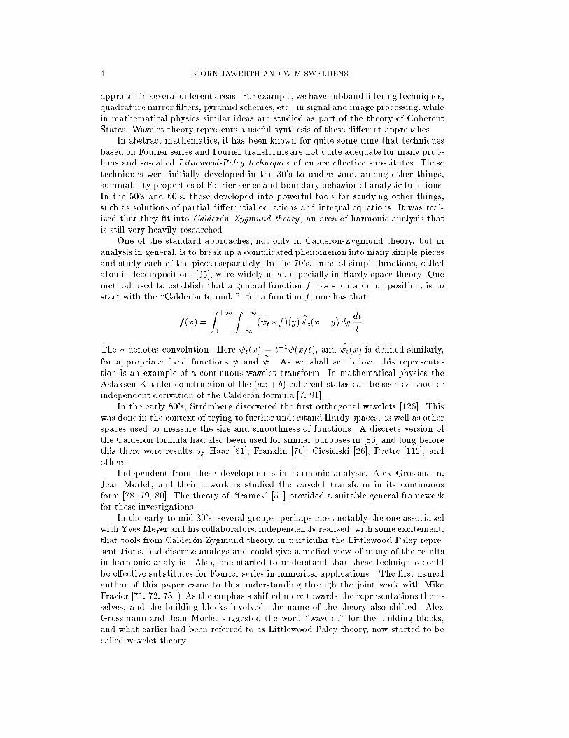
Fig. 1. The subband �ltering scheme.
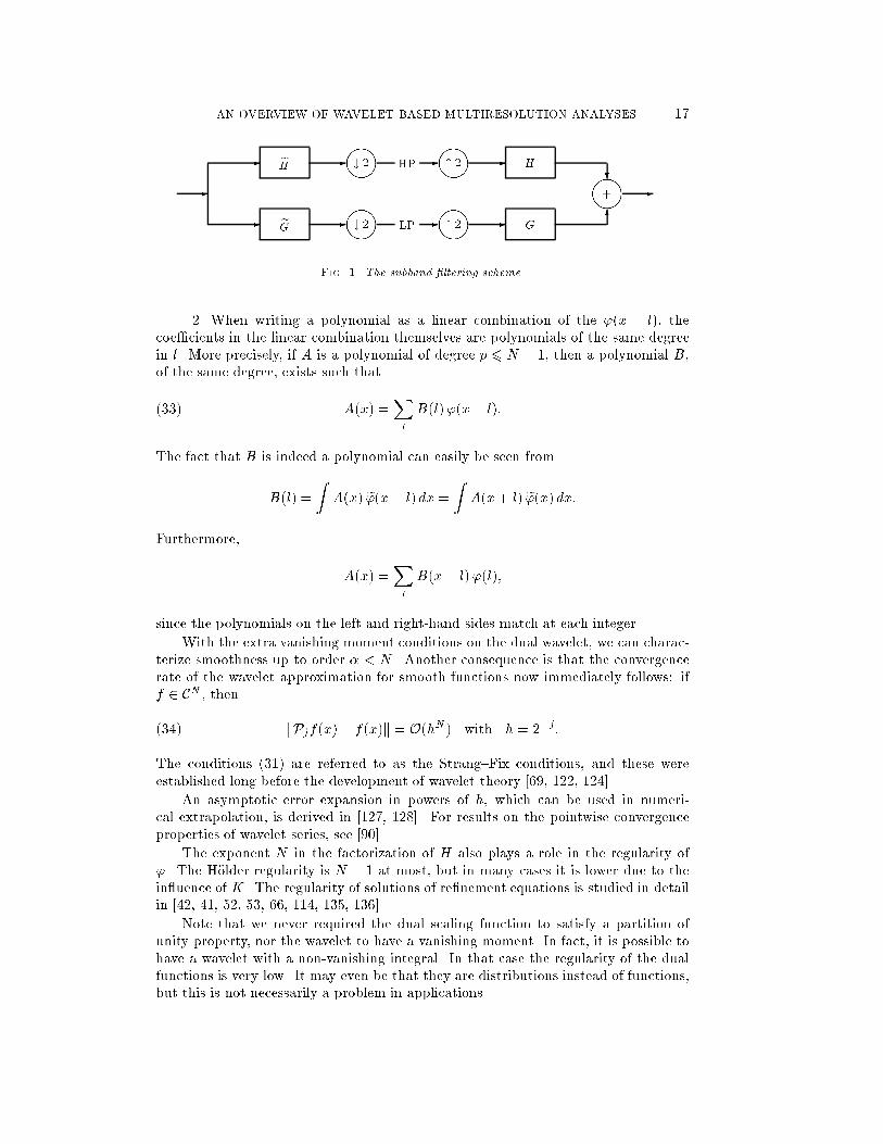
2. When writing a polynomial as a linear combination of the '(x � l), thecoe�cients in the linear combination themselves are polynomials of the same degreein l. More precisely, if A is a polynomial of degree p 6 N � 1, then a polynomial B,of the same degree, exists such that
A(x) =Xl
B(l)'(x� l):(33)
The fact that B is indeed a polynomial can easily be seen from
B(l) =
ZA(x) e'(x� l) dx = Z A(x+ l) e'(x) dx:
Furthermore,
A(x) =Xl
B(x� l)'(l);
since the polynomials on the left and right-hand sides match at each integer.
With the extra vanishing moment conditions on the dual wavelet, we can charac-terize smoothness up to order � < N . Another consequence is that the convergencerate of the wavelet approximation for smooth functions now immediately follows: iff 2 CN , then
kPjf(x)� f(x)k = O(hN) with h = 2�j:(34)
The conditions (31) are referred to as the Strang{Fix conditions, and these wereestablished long before the development of wavelet theory [69, 122, 124].
An asymptotic error expansion in powers of h, which can be used in numeri-cal extrapolation, is derived in [127, 128]. For results on the pointwise convergenceproperties of wavelet series, see [90].
The exponent N in the factorization of H also plays a role in the regularity of'. The H�older regularity is N � 1 at most, but in many cases it is lower due to thein uence of K. The regularity of solutions of re�nement equations is studied in detailin [42, 41, 52, 53, 66, 114, 135, 136].
Note that we never required the dual scaling function to satisfy a partition ofunity property, nor the wavelet to have a vanishing moment. In fact, it is possible tohave a wavelet with a non-vanishing integral. In that case the regularity of the dualfunctions is very low. It may even be that they are distributions instead of functions,but this is not necessarily a problem in applications.

18 BJORN JAWERTH AND WIM SWELDENS
�n;l �n�1;l
n�1;l
�n�2;l
n�2;l
: : : �1;l
1;l
�0;l
0;l
-�����
-�����
-�����
-�����
Fig. 2. The decomposition scheme.
�0;l
0;l
�1;l
1;l
�2;l
2;l
: : : �n�1;l
n�1;l
�n;l-
@@@@R
-
@@@@R
-
@@@@R
-
@@@@R
Fig. 3. The reconstruction scheme.
9. The fast wavelet transform. Since Vj is equal to Vj�1 �Wj�1, a functionvj 2 Vj can be written uniquely as the sum of a function vj�1 2 Vj�1 and a functionwj�1 2Wj�1:
vj(x) =Xk
�j;k 'j;k(x) = vj�1(x) +wj�1(x)
=Xl
�j�1;l 'j�1;l(x) +Xl
j�1;l j�1;l(x):
In other words, we have two representations of the function vj , one as an element inVj and associated with the sequence f�j;kg, and another as a sum of elements in Vj�1and Wj�1 and associated with the sequences f�j�1;kg and f j�1;kg. The followingrelations show how to pass between these representations. By (25),
�j�1;l = h vj ; e'j�1;l i = p2 h vj ;Xk
ehk�2l e'j;k i=p2Xk
ehk�2l �j;k;(35)
and, similarly,
j�1;l =p2Xk
egk�2l �j;k:(36)
The opposite direction, from the �j�1;l and the j�1;l to the �j;k, is equally easy.Using (30) we have
�j;k =p2Xl
hk�2l �j�1;l +p2Xl
gk�2l j�1;l:(37)

AN OVERVIEW OF WAVELET BASED MULTIRESOLUTION ANALYSES 19
When applied recursively, these formulae de�ne the fast wavelet transform; the re-lations (35) and (36) de�ne the forward transform, while (37) de�nes the inversetransform.
Now, from the fact thatH(0) = G(�) = 1 andG(0) = H(�) = 0, we see thatH(!)acts like a low pass �lter for the interval [0; �=2] andG(!) similarly behaves like a bandpass �lter for the interval [�=2; �]. Equation (8) (respectively (12)) then implies thatthe major part of the energy of the functions in V0 (respectively W0) is concentratedin the intervals [0; �] (respectively [�; 2�]). The basic behavior of the dual functionsis the same. In an approximate sense, this means that the wavelet expansion splitsthe frequency space into dyadic blocks [2j�; 2j+1�] with j 2 Z [103, 104].
In signal processing this idea is known as subband �ltering, or, more speci�cally,as quadrature mirror �ltering. Quadrature mirror �lters were studied before wavelettheory. The decomposition step consists of applying a low-pass ( eH) and a band-
pass ( eG) �lter followed by downsampling (# 2) (i.e. retaining only the even indexsamples), see Figure 1. The reconstruction consists of upsampling (" 2) (i.e. puttinga zero between every two samples) followed by �ltering and addition. One can showthat the conditions (27) correspond to the exact reconstruction of a subband �lteringscheme. More details about this can be found in [115, 132, 133, 134].
An interesting problem now is: given a function f , determine, with a certainaccuracy and in a computationally favorable way, the coe�cients �n;l of a function inthe space Vn, which are needed to start the fast wavelet transform. A trivial solutioncould be
�n;l = f(l=2n):
Other sampling procedures, such as (quasi-)interpolation and quadrature formulaewere proposed in [1, 2, 85, 120, 128, 138].
An implementation of a fast wavelet transform in pseudo code is given in theappendix.
10. Examples of wavelets. Now that we have discussed the essentials of wave-let multiresolution analysis, we take a look at some important properties of wavelets.
Orthogonality. Orthogonality is convenient to have in many situations, e.g. itdirectly links the L2 norm of a function to the norm of its wavelet coe�cients by
kfk =sX
j;l
2j;l:
In the biorthogonal case these two quantities are only equivalent. Another advantageof orthogonal wavelets is that the fast wavelet transform is a unitary transformation(i.e. its adjoint is its inverse). Consequently, its condition number is equal to 1, whichis the optimal case. (Recall that the condition number of a linear transformation Ais de�ned as kAk:kA�1k). This is of importance in numerical calculations. It meansthat an error present in the initial data will not grow under the transformation, andthat stable numerical computations are possible.
If the multiresolution analysis is orthogonal (remember that this includes semior-thogonal wavelets), the projection operators onto the di�erent subspaces yield optimalapproximations in the L2 sense.

20 BJORN JAWERTH AND WIM SWELDENS
Compact support. If the scaling function and wavelet are compactly supported,the �lters H and G are �nite impulse response �lters, so that the summations inthe fast wavelet transform are �nite. This obviously is of use in implementations. Ifthey are not compactly supported, a fast decay is desirable so that the �lters can beapproximated reasonably by �nite impulse response �lters.
Rational coe�cients. For computer implementations it is of use if the �lter co-e�cients hk and gk are rationals or, even better, dyadic rationals. Multiplicationby a power of two on a computer corresponds to shifting bits, which is a very fastoperation.
Symmetry. If the scaling function and wavelet are symmetric, then the �lters havegeneralized linear phase. The absence of this property can lead to phase distortion.This is important in signal processing applications.
Smoothness. The smoothness of wavelets plays an important role in compressionapplications. Compression is usually achieved by setting small coe�cients j;l tozero, and thus leaving out a component j;l j;l(x) from the original function. Ifthe original function represents an image and the wavelet is not smooth, the errorcan easily be detected visually. Note that the smoothness of the primary functionsis more important to this aspect than that of the dual. Also, a higher degree ofsmoothness corresponds to better frequency localization of the �lters. Finally, smoothbasis functions are desired in numerical analysis applications where derivatives areinvolved.
Number of vanishing moments of the dual wavelet. We saw earlier that this isimportant in singularity detection and characterization of smoothness spaces. Also,it determines the convergence rate of wavelet approximations of smooth functions.Finally, the number of vanishing moments of the dual wavelet is connected to thesmoothness of the wavelet (and vice versa).
Analytic expressions. As previously noted, an analytic expression for a scalingfunction or wavelet does not always exists but in some cases it is available and niceto have. In harmonic analysis, analytic expressions of the Fourier transform areparticularly useful.
Interpolation. If the scaling function satis�es
'(k) = �k for k 2 Z;
then it is trivial to �nd the function of Vj that interpolates data sampled on a gridwith spacing 2�j , since the coe�cients are equal to the samples.
As could be expected, it is not possible to construct wavelets that have all theseproperties and there is a trade-o� between them. We now take a look at severalcompromises.
Examples of orthogonal wavelets.
(i) Two simple examples of orthogonal scaling functions are the box function�[0;1](x) and the Shannon sampling function sinc(�x). The orthogonality conditionsare easy to verify, either in the time or frequency space. The corresponding waveletfor the box function is the Haar wavelet
Haar(x) = �[0;1=2](x)� �[1=2;1](x);

AN OVERVIEW OF WAVELET BASED MULTIRESOLUTION ANALYSES 21
and the Shannon wavelet is
Shannon(x) =sin(2�x)� sin(�x)
�x:
These two, however, are not very useful in practice, since the �rst has very lowregularity and the second has very slow decay.
(ii) A more interesting example is theMeyer wavelet and scaling function [106].These functions belong to C1 and have faster than polynomial decay. Their Fouriertransform is compactly supported. The scaling function and wavelet are symmetricaround 0 and 1=2, respectively, and the wavelet has an in�nite number of vanishingmoments.
(iii) The Battle-Lemari�e wavelets are constructed by orthogonalizing B{splinefunctions using (20) and have exponential decay [12, 95]. The wavelet with N van-ishing moments is a piecewise polynomial of degree N � 1 that belongs to CN�2.
(iv) Probably the most frequently used orthogonal wavelets are the original Dau-bechies wavelets [47, 49]. They are a family of orthogonal wavelets indexed by N 2N,where N is the number of vanishing wavelet moments. They are supported on an in-terval of length 2N � 1. A disadvantage is that, except for the Haar wavelet (whichhas N = 1), they cannot be symmetric or antisymmetric. Their regularity increaseslinearly with N and is approximately equal to 0:2075N for large N . In [137] a dif-ferent family with regularity asymptotically equal to 0:3N was presented. In [50]three variations of the original family, all with orthogonal and compactly supportedfunctions, are constructed:
1. The previous construction does not lead to a unique solution if N and thesupport length are �xed. One family is constructed by choosing, for each N , thesolution with closest to linear phase (or closest to symmetry). In fact, the originalfamily corresponds to choosing the extremal phase.
2. Another family has more regularity, at the price of a slightly larger supportlength (2N + 1).
3. In a third family, the scaling function also has vanishing moments (Mp = 0for 0 < p < N). This is of use in numerical analysis applications where inner productsof arbitrary functions with scaling functions have to be calculated very fast [17]. Theirconstruction was asked by Ronald Coifman and Ingrid Daubechies therefore namedthem coi ets . They are supported on an interval with length 3N � 1.
Examples of biorthogonal wavelets.
(i) Biorthogonal wavelets were constructed by Albert Cohen, Ingrid Daubechiesand Jean-Christophe Feauveau in [31]. Here �(!) is chosen equal to e�i!, and thus
G(!) = �e�i! eH(! + �) and eG(!) = �e�i!H(! + �):
In one of the families constructed in [31], the scaling functions are the cardinal B-splines and the wavelets too are spline functions. All functions including the dualones have compact support and linear phase. Moreover, all �lter coe�cients aredyadic rationals. A disadvantage is that for small �lter lengths, the dual functionshave very low regularity.
(ii) Semiorthogonal spline wavelets were constructed by Charles Chui and Jian-zhong Wang in [23, 24, 25]. The scaling functions are cardinal B{splines of orderm and the wavelet functions are splines with support [0; 2m � 1]. All primary anddual functions still have generalized linear phase and all coe�cients used in the fast

22 BJORN JAWERTH AND WIM SWELDENS
Table 1
A quick comparison of wavelet families.
wavelet compact support analytic expression symmetry orthogonality compact
family primary dual primary dual semi full support b a x x o o o x x o
b x x x o x o o o
c x o x x x x o o
d o o o o x x x x
e o o x x x x x o
a: Daubechies' orthogonal wavelets
b: biorthogonal spline wavelets
c: semiorthogonal spline wavelets
d: Meyer wavelet
e: orthogonal spline wavelets
wavelet transform are rationals. A powerful feature here is that analytic expressionsfor the wavelet, scaling function, and dual functions are available. A disadvantageis that the dual functions do not have compact support, but have exponential decayinstead. The same wavelets, but in a di�erent setting, were also derived by AkramAldroubi, Murray Eden and Michael Unser in [129, 131]. They also showed that forN going to in�nity, the spline wavelets converge to Gabor functions [130].
(iii) Other semiorthogonal wavelets can be found in [89, 109, 110, 113]. A char-acterization of all semiorthogonal wavelets is given in [1, 2].
The properties of some of the orthogonal, biorthogonal and semiorthogonal wave-let families are summarized in Table 1.
Examples of interpolating scaling functions.
(i) The Shannon sampling function
'Shannon =sin(�x)
�x;
is an interpolating scaling function. It is band limited, but it has very slow decay.(ii) An interpolating scaling function, whose translates also generate V0, can be
found by letting
b'interpol(!) = b'(!)Xl
'(l)e�i!l;
provided that the denominator does not vanish [1, 2, 129, 138]. Even if ' is compactlysupported, 'interpol is in general not compactly supported. The cardinal spline inter-polants of even order are constructed this way [118].
(iii) An interpolating scaling function can also be constructed from a pair ofbiorthogonal scaling functions as
'interpol(x) =
Z +1
�1
'(y + x) e'(y) dy:The interpolation property immediately follows from the biorthogonality condition.In the case of an orthogonal scaling function this is just its autocorrelation func-tion. The interpolating function and its translates do not generate the same space

AN OVERVIEW OF WAVELET BASED MULTIRESOLUTION ANALYSES 23
as ' and its translates. This construction, starting from the Daubechies orthogonalor biorthogonal wavelets, yields a family of interpolating functions which had beenstudied earlier by Gilles Deslauriers and Serge Dubuc in [56, 57]. These functions aresmooth and compactly supported. More information can also be found in [61, 117]. Anatural choice for the wavelet here is (x) = '(2x�1) and this is a typical example ofa wavelet with a non-vanishing integral. The dual scaling function is a Dirac impulseand the dual wavelet is a linear combination of Dirac impulses (and has several van-ishing moments). We still have a fast wavelet transform with �nite impulse response�lters.
(iv) Also wavelets can be interpolating. In [2] wavelets that are both symmetricaland interpolating were constructed.
11. Wavelets on an interval. So far we have been discussing wavelet theoryon the real line (and its higher dimensional analogs). For many applications, thefunctions involved are only de�ned on a compact set, such as an interval or a square,and to apply wavelets then requires some modi�cations.
11.1. Simple solutions. To be speci�c, let us discuss the case of the unit inter-val [0; 1]. Given a function f on [0; 1], the most obvious approach is to set f(x) = 0outside [0; 1], and then use wavelet theory on the line. However, for a general func-tion f this \padding with 0s" introduces discontinuities at the endpoints 0 and 1;consider for example the simple function f(x) = 1, x 2 [0; 1]. Now, as we have saidearlier, wavelets are e�ective for detecting singularities, so arti�cial ones are likely tointroduce signi�cant errors.
Another approach, which is often better, is to consider the function to be periodicwith period 1, f(x + 1) = f(x). Expressed in another way, we assume that thefunction is de�ned on the torus and identify the torus with [0; 1]. Wavelet theoryon the torus parallels that on the line. In fact, note that if f has period 1, thenthe wavelet coe�cients on a given scale satisfy h f; j;k i = h f; j;k+2j i , k 2 Z,j � 0. This simple observation readily allows us to rewrite wavelet expansions onthe line as analogous ones on the torus, with wavelets de�ned on [0; 1]. A periodicmultiresolution analysis on the interval [0; 1] can be constructed by periodizing thebasis functions as follows,
'�j;l(x) = �[0;1](x)Xm
'j;l(x+m) for 0 6 l < 2j and j > 0:(38)
If the support of 'j;l(x), is a subset of [0; 1], then '�j;l(x) = 'j;l(x). Otherwise'j;l(x) is chopped into pieces of length 1, which are shifted onto [0; 1] and added
up, yielding '�j;l(x). Similar de�nitions hold for �j;l, e'�j;l and e �j;l. The algorithmin the appendix describes the periodic fast wavelet transform. This \wrap around"procedure is satisfactory in many situations (and certainly takes care of functions likef(x) = 1, x 2 [0; 1]). However, unless the behavior of the function f at 0 matchesthat at 1, the periodic version of f has singularities there. A simple function likef(x) = x, x 2 [0; 1], gives a good illustration of this.
A third method, which works if the basis functions are symmetric, is to usere ection across the edges. This preserves continuity, but introduces discontinuitiesin the �rst derivative. This solution is sometimes satisfactory in image processingapplications.
11.2. Meyer's boundary wavelets. What really is needed, are wavelets in-trinsically de�ned on [0; 1]. We sketch a construction of orthogonal wavelets on [0; 1],

24 BJORN JAWERTH AND WIM SWELDENS
recently presented by Yves Meyer [107]. We start from an orthogonal Daubechiesscaling function with 2N non-zero coe�cients:
'(x) = 2
2N�1Xk=0
hk '(2x� k):(39)
It is easy to see that closfx : '(x) 6= 0g = [0; 2N � 1], and, as a consequence,
Bj;k = closfx : 'j;k(x) 6= 0g = [2�jk; 2�j(k + 2N � 1)]:(40)
This implies that for su�ciently small scales 2�j, j � j0, a function 'j;k can onlyintersect at most one of the endpoints 0 or 1. Let us restate this in a di�erent way.De�ne the set of indices
Sj = fk : Bj;k \ (0; 1) 6= ;g:
We de�ne three subsets of this set containing the indices of the basis functions at theleft boundary, in the interior, and at the right boundary:
S(1)
j = fk : 0 2 B�j;kg
S(2)
j = fk : B�j;k � (0; 1)g
S(3)
j = fk : 1 2 B�j;kg:
Here E� denotes the interior of the set E. For su�ciently large j the sets S(1)
j and
S(3)
j are disjoint and
Sj = S(1)
j [ S(2)
j [ S(3)
j :
It is easy to write down what these sets are more explicitly:
S(1)
j = fk : �2N + 2 6 k 6 �1g
S(2)
j = fk : 0 6 k 6 2j � 2N + 1g
S(3)
j = fk : 2j � 2N + 2 6 k 6 2j � 1g:
Note, in particular, that the sets S(1)
j and S(3)
j contain the indices of 2N�2 functions,independently of j. We now let V
[0;1]j denote the restriction of functions in Vj :
V[0;1]j = ff : f(x) = g(x); x 2 [0; 1]; for some function g 2 Vjg:
Clearly, since the Vj form an increasing sequence of spaces,
V[0;1]j � V
[0;1]j+1 ;
and V[0;1]j , j � j0, form a multiresolution analysis of L2([0; 1]). It is also obvious
that the functions in f'(x � l)j[0;1] : l 2 Sjg span V[0;1]j . Here g(x) j[0;1] denotes
the restriction of g(x) to [0; 1]. Not quite as obvious is the fact that the functions in
this collection are linearly independent, and hence form a basis for V[0;1]j . In order

AN OVERVIEW OF WAVELET BASED MULTIRESOLUTION ANALYSES 25
to obtain an orthonormal basis, we may argue as follows. As long as the function'j;k lives entirely inside [0; 1], restricting it to [0; 1] has no e�ect. In particular, the
functions 'j;k, k 2 S(2)j are still pairwise orthogonal. A key observation now is that
for k 2 S(1)j , l 2 S(2)j [ S(3)
j ,
h'j;k; 'j;l i [0;1] =Z 1
0
'j;k(x)'j;l(x) dx =
Z +1
�1
'j;k(x)'j;l(x) dx = 0;(41)
and similarly when k 2 S(3)
j , l 2 S(2)
j [ S(1)j . We see that the three collections
f'(x� l)j[0;1] : l 2 S(1)
j g, f'(x� l)j[0;1] : l 2 S(2)
j g, and f'(x � l)j[0;1] : l 2 S(3)
j g aremutually orthogonal. So, since the functions in f'(x� l)j[0;1] : l 2 S
(2)
j g already forman orthonormal set, there only remains to separately orthogonalize the functions in
f'(x� l)j[0;1] : l 2 S(1)j g and in f'(x� l)j[0;1] : l 2 S(3)j g. This is easily accomplishedwith a Gram-Schmidt procedure.
Now, if we let W[0;1]j denote the restriction of functions in Wj to [0; 1], then we
have that
V[0;1]j+1 = V
[0;1]j +W
[0;1]j :(42)
So, the basis elements in V[0;1]j together with the restriction of the wavelets j;k to
[0; 1] span V[0;1]j+1 . However, there are 2
j + 2N � 2 wavelets that intersect [0; 1], and,
since dimV[0;1]j+1 � dimV
[0;1]j = 2j we have too many functions. The restrictions of
the wavelets in Wj that live entirely inside [0; 1] are still mutually orthogonal and, by
an observation similar to (41), they are also orthogonal to V[0;1]j . There are 2N � 2
wavelets whose support intersects an endpoint. However, we only need N � 1 basisfunctions at each endpoint. One can now use (30) to write out the dependencies,and construct N � 1 basis functions at each endpoint. After that we just apply a
Gram-Schmidt procedure again, and we have an orthonormal basis for W[0;1]j .
This elegant construction of Yves Meyer has a couple of disadvantages. Amongthe functions 'j;k that intersect [0; 1] there are some that are almost zero there. Hence,the set f'j;kgk2Sj is almost linearly dependent, and, as a consequence, the conditionnumber of the matrix, corresponding to the change of basis from f'j;kgk2Sj to the
orthonormal one, becomes quite large. Furthermore, we have dimV[0;1]j 6= dimW
[0;1]j ,
which means that there is an inherent imbalance between the spaces V[0;1]
j andW[0;1]
j ,which is not present in the case of the whole real line.
11.3. Dyadic boundary wavelets. As we noted earlier (33) all polynomials ofdegree 6 N � 1 can be written as linear combinations of the 'j;l for l 2 Z. Hence,
the restriction of such polynomials to [0; 1] are in V[0;1]j . Since this fact is directly
linked to many of the approximation properties of wavelets, any construction of amultiresolution analysis on [0; 1] should preserve this. The construction in [5, 32, 33]uses this as a starting point and is slightly di�erent from the one by Yves Meyer.Let us brie y describe this construction as well. Again we start with an orthogonalDaubechies scaling function ' with 2N non-zero coe�cients, and assume that we havepicked the scale �ne enough so that the endpoints are independent as before. By (33)and, since the f'j;kg is an orthonormal basis for Vj , each monomial x�, � 6 N � 1,has the representation x� =
Pk hx�; 'j;k i'j;k(x). The restriction to [0; 1] can then
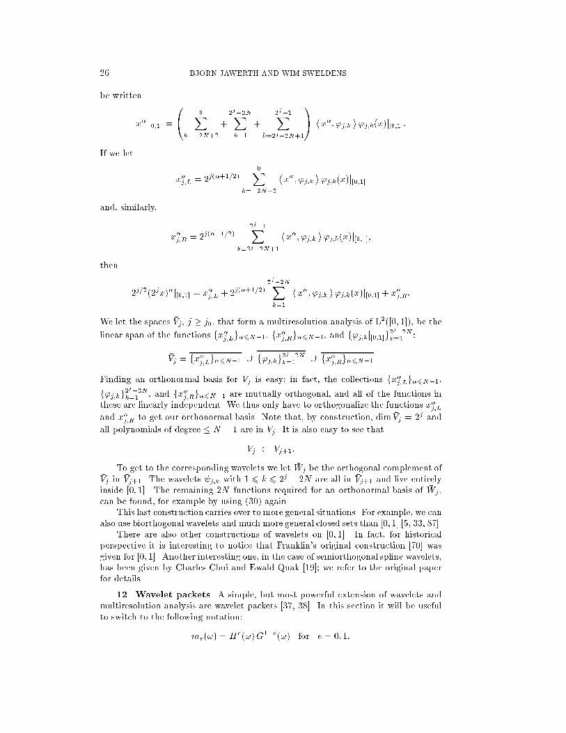
26 BJORN JAWERTH AND WIM SWELDENS
be written
x�j[0;1] =
0@ 0Xk=�2N+2
+
2j�2NXk=1
+
2j�1Xk=2j�2N+1
1A hx�; 'j;k i'j;k(x)j[0;1]:
If we let
x�j;L = 2j(�+1=2)0X
k=�2N+2
hx�; 'j;k i'j;k(x)j[0;1]
and, similarly,
x�j;R = 2j(�+1=2)2j�1X
k=2j�2N+1
hx�; 'j;k i'j;k(x)j[0;1];
then
2j=2(2jx)�j[0;1] = x�j;L + 2j(�+1=2)2j�2NXk=1
hx�; 'j;k i'j;k(x)j[0;1] + x�j;R:
We let the spaces �Vj , j � j0, that form a multiresolution analysis of L2([0; 1]), be the
linear span of the functions fx�j;Lg�6N�1, fx�j;Rg�6N�1, and f'j;kj[0;1]g2j�2Nk=1 :
�Vj = fx�j;Lg�6N�1 [ f'j;kg2j�2Nk=1 [ fx�j;Rg�6N�1
Finding an orthonormal basis for �Vj is easy; in fact, the collections fx�j;Lg�6N�1,f'j;kg2
j�2Nk=1 , and fx�j;Rg�6N�1 are mutually orthogonal, and all of the functions in
these are linearly independent. We thus only have to orthogonalize the functions x�j;Land x�j;R to get our orthonormal basis. Note that, by construction, dim �Vj = 2j and
all polynomials of degree � N � 1 are in �Vj . It is also easy to see that
�Vj � �Vj+1:
To get to the corresponding wavelets we let �Wj be the orthogonal complement of�Vj in �Vj+1. The wavelets j;k with 1 6 k 6 2j � 2N are all in �Vj+1 and live entirelyinside [0; 1]. The remaining 2N functions required for an orthonormal basis of �Wj ,can be found, for example by using (30) again.
This last construction carries over to more general situations. For example, we canalso use biorthogonal wavelets and much more general closed sets than [0; 1] [5, 33, 87].
There are also other constructions of wavelets on [0; 1]. In fact, for historicalperspective it is interesting to notice that Franklin's original construction [70] wasgiven for [0; 1]. Another interesting one, in the case of semiorthogonal spline wavelets,has been given by Charles Chui and Ewald Quak [19]; we refer to the original paperfor details.
12. Wavelet packets. A simple, but most powerful extension of wavelets andmultiresolution analysis are wavelet packets [37, 38]. In this section it will be usefulto switch to the following notation:
me(!) = He(!)G1�e(!) for e = 0; 1:

AN OVERVIEW OF WAVELET BASED MULTIRESOLUTION ANALYSES 27
V0 W0
V1 W1
V2 W2
V3
��@@R
��@@R ��@@R
�� @@R ��@@R ��@@R ��@@R
Fig. 4. Wavelet packets scheme.
The fundamental observation is the following fact, called the splitting trick [22, 30,106]:Suppose that the set of functions ff(x � k) j k 2 Zg is a Riesz basis for its closed
linear span S. Then the functions
f0k =1p2f0(x=2� k) and f1k =
1p2f1(x=2� k) for k 2 Z;
also constitute a Riesz basis for S, where
bfe(!) = me(!=2) bf(!=2):We see that the classical multiresolution analysis is obtained by splitting Vj with
this trick into Vj�1 and Wj�1 and then doing the same for Vj�1 recursively. Thewavelet packets are the basis functions that we obtain if we also use the splitting trickon theWj spaces. So starting from a space Vj , we obtain, after applying the splittingtrick L times, the basis functions
Le1;:::;eL;j;k(x) = 2(j�L)=2 Le1;:::;eL(2j�Lx� k);
with
b Le1;:::;eL(!) =LYi=1
mei(2�i !) b'(2�L!):
So, after L splittings, we have 2L basis functions and their translates over integermultiples of 2L�j as a basis of Vj . The connection between the wavelet packets andthe wavelet and scaling functions is
' = L0;:::;0 and = L1;0;:::;0:
However, we do not necessarily have to split each subspace at every stage. InFigure 4 we give a schematical representation of a space and its subspaces after usingthe splitting on 3 levels. The top rectangle represents the space V3 and each otherrectangle corresponds to a certain subspace of V3 generated by wavelet packets. Theslanted lines between the rectangles indicate the splitting, the left referring to the�lter m0 and the right to m1. The dashed rectangles then correspond to the wavelet

28 BJORN JAWERTH AND WIM SWELDENS
multiresolution analysis V3 = V0�W0�W1�W2. The bold rectangles correspond toa possible wavelet packet splitting and a basis with functions�
10(4x� k); 21;1(2x� k); 30;0;1(x� k); 31;0;1(x� k) j k 2 Z:
For the dual functions, a similar procedure has to be followed.
In the Fourier domain, the splitting trick corresponds to dividing the frequencyinterval essentially represented by the original space into two parts. So the waveletpackets allow more exibility in adapting the basis to the frequency contents of asignal.
It is easy to develop a fast wavelet packet transform. It just involves applyingthe same low and band pass �lters also to the coe�cient of functions of Wj againin an iterative manner. This means that, starting from M samples, we construct afull binary tree with (M log2M) entries. The power of this construction lies in thefact that we have much more freedom in deciding which basis functions we will useto represent the given function. We can choose to use the set of M coe�cients of thetree to represent the function that is optimal with respect to a certain criterion. Thisprocedure is called best basis selection, and one can design fast algorithms that makeuse of the tree structure. The particular criterion is determined by the application,and which basis functions that will end up in the basis depends on the data.
For applications in image processing, entropy-based criteria were proposed in[40]. The best basis selection in that case has a numerical complexity of O(M).Applications in signal processing can be found in [36, 139].
This wavelet packets construction can also be combined with wavelets on aninterval and wavelets in higher dimensions [55].
13. Multidimensional wavelets. Up till now we have focused on functions ofone variable and the one-dimensional situation. However, there are also wavelets inhigher dimensions. A simple way to obtain these is to use tensor products. To �xideas, let us consider the case of the plane. Let
�(x; y) = '(x)'(y) = ' '(x; y);
and de�ne
V0 = ff : f(x; y) =Xk1;k2
�k1;k2 �(x� k1; y � k2); � 2 l2(Z2)g:
Of course, if f'(x� l) j l 2 Zg is an orthonormal set, then f�(x� k1; y � k2)g forman orthonormal basis for V0. By dyadic scaling we obtain a multiresolution analysisof L2(R2). The complement W0 of V0 in V1 is similarly generated by the translatesof the three functions
(1) = ' ; (2) = '; and (3) = :(43)
There is another, perhaps even more straightforward, wavelet decomposition inhigher dimensions. By carrying out a one-dimensional wavelet decomposition for eachvariable separately, we obtain
f(x; y) =Xi;l
Xj;k
h f; i;l j;k i i;l j;k(x; y):(44)

AN OVERVIEW OF WAVELET BASED MULTIRESOLUTION ANALYSES 29
Note that the functions i;l j;k involve two scales, 2�i and 2�j , and each ofthese functions are (essentially) supported on a rectangle. The decomposition (44) istherefore called the rectangular wavelet decomposition of f while the functions in (43)are the basis functions of the square wavelet decomposition. For both decompositions,the corresponding fast wavelet transform consists of applying the one-dimensional fastwavelet transform to the rows and columns of a matrix.
These simple constructions are insu�cient in many cases. What we need some-times are wavelets intrinsically constructed for higher dimensions. One of the inter-esting problems here is how to split a space into complementary subspaces. In theunivariate case we split into two spaces, each with essentially the same \size." If weuse the square tensor product basis in d dimensions, we split into 2d subspaces, 2d�1of which are spanned by wavelets. There are several constructions of nonseparablewavelets that use this kind of splitting. One of the problems here is, given the scal-ing function, is there an easy way, cf. (19), to �nd the wavelets? This was studiedin [54, 113, 121]. Another idea is to still try to split into just two subspaces. Thisinvolves the use of di�erent lattices [99]. In the bivariate case, Ingrid Daubechiesand Albert Cohen constructed smooth, compactly supported, biorthogonal wavelets,using ideas from the univariate construction [29].
By now, there is a lot of material about multivariate wavelets. However, we shallleave this topic for now and just mention some other possibilities such as hexagonallattices, and Cli�ord valued wavelets [6, 9, 34].
14. Applications.
14.1. Data compression. One of the most common applications of wavelettheory is data compression. There are two basic kinds of compression schemes: losslessand lossy. In the case of lossless compression one is interested in reconstructing thedata exactly, without any loss of information. We consider here lossy compression.This means we are ready to accept an error, as long as the quality after compression isacceptable. With lossy compression schemes we potentially can achieve much highercompression ratios than with lossless compression.
To be speci�c, let us assume that we are given a digitized image. The compressionratio is de�ned as the number of bits the initial image takes to store on the computerdivided by the number of bits required to store the compressed image. The interestin compression in general has grown as the amount of information we pass aroundhas increased. This is easy to understand when we consider the fact that to store amoderately large image, say a 512� 512 pixels, 24 bit color image, takes about 0.75MBytes. This is only for still images; in the case of video, the situation becomes evenworse. Then, we need this kind of storage for each frame, and we have somethinglike 30 frames per second. There are several reasons other than just the storagerequirement for the interest in compression techniques. However, instead of goinginto this, let us now look at the connection with wavelet theory.
First, let us de�ne, somewhat mathematically, what we mean by an image. Letus for simplicity discuss an L�L grayscale image with 256 grayscales (i.e. 8 bit). Thiscan be considered to be a piecewise constant function f de�ned on a square
f(x; y) = pij 2N; for i 6 x < i+ 1 and j 6 y < j + 1 and 0 6 i; j < L;
where 0 6 pij 6 255. Now, one of the standard procedures for lossy compression isthrough transform coding, see Figure 5. The most common transform used in thiscontext is the \Discrete Cosine Transform", which uses a Fourier transform of the

30 BJORN JAWERTH AND WIM SWELDENS
original
imageforward
transformcoding M
coe�cientsinverse
transformreconstructed
image- - - -
Fig. 5. Image transform coding.
image f . However, we are more interested in the case when the transform is the fastwavelet transform.
There are in fact several ways to use the wavelet transform for compression pur-poses [101, 102]. One way is to consider compression to be an approximation problem[58, 59]. More speci�cally, let us �x an orthogonal wavelet . Given an integerM > 1,we try to �nd the \best" approximation of f by using a representation
fM (x) =Xkl
bjk jk(x) with M non-zero coe�cients bjk:(45)
The basic reason why this potentially might be useful is that each wavelet picks upinformation about the image f essentially at a given location and at a given scale.Where the image has more interesting features, we can spend more coe�cients, andwhere the image is nice and smooth we can use fewer and still get good quality ofapproximation. In other words, the wavelet transform allows us to focus on the mostrelevant parts of f . Now, to give this mathematical meaning we need to agree on anerror measure. Ideally, for image compression we should use a norm that correspondsas closely as possible to the human eye [58]. However, let us make it simple anddiscuss the case of L2.
So we are interested in �nding an optimal approximation minimizing the errorkf � fMkL2 . Because of the orthogonality of the wavelets this equals0
@Xjk
j h f; jk i � bjkj21A
1=2
:(46)
A moment's thought, reveals that the best way to pick M non-zero coe�cients bjk,making the error as small as possible, is by simply picking the M coe�cients withlargest absolute value, and setting bj;k = h f; jk i for these numbers. This thenyields the optimal approximation foptM .
Another fundamental question is which images can be approximated well by usingthe procedure just sketched. Let us take this to mean that the error satis�es
kf � foptM kL2 = O(M��);(47)
for some � > 0. The larger �, the faster the error decays asM increases and the fewercoe�cients are generally needed to obtain an approximation within a given error. Theexponent � can be found easily, in fact it can be shown that
0@XM�1
(M�kf � foptM kL2)p 1
M
1A
1=p
� (Xjk
j h f; jk i jp)1=p(48)
with 1=p = 1=2 + �. The maximal � for which (47) is valid can be estimated by�nding the smallest p for which the right-hand side of (48) is �nite. The expression

AN OVERVIEW OF WAVELET BASED MULTIRESOLUTION ANALYSES 31
on the right is one of many equivalent norms on the Besov space _B2�;pp (Besov spaces
are smoothness spaces generalizing the Lipschitz continuous functions). The � inthe left-hand side of (48) is actually not exactly the same as in (47). However, forpractical purposes, the di�erence is of no consequence.
14.2. Operator analysis. As mentioned earlier, interest in wavelets histori-cally grew from the fact that they are e�ective tools for studying problems in partialdi�erential equations and operator theory. More speci�cally, they are useful for un-derstanding properties of so-called Calder�on-Zygmund operators .
Let us �rst make a general observation about the representation of a linear oper-ator T and wavelets. Suppose that f has the representation
f(x) =Xjk
h f; jk i jk(x):
Then,
Tf(x) =Xjk
h f; jk iT jk(x);
and, using the wavelet representation of the function T jk(x), this equals
Xjk
h f; jk iXil
hT jk; il i il(x) =Xil
0@X
jk
hT jk; il i h f; jk i
1A il(x):
In other words, the action of the operator T on the function f is directly trans-lated into the action of the in�nite matrix AT = f hT jk; il i gil;jk on the sequencef h f; jk i gjk. This representation of T as the matrix AT is often referred to as the\standard representation" of T [17]. There is also a \nonstandard representation".For virtually all linear operators there is a function (or, more generally, a distribution)K such that
Tf(x) =
ZK(x; y)f(y) dy:
The nonstandard representation of T is now simply the (two-dimensional) wavelet
coe�cients of the kernel K, using the square decomposition f hK;(j)
k1;k2i g (again,
we have more than one wavelet function in two dimensions), while the standard rep-resentation corresponds to the rectangular decomposition.
Let us then brie y discuss the connection with Calder�on-Zygmund operators.Consider a typical example. Let H be the Hilbert transform,
Hf(x) =1
�
Z 1
�1
f(s)
x� s ds:
The basic idea now is that the wavelets jk are approximate eigenfunctions for this,as well as for many other related (Calder�on-Zygmund) operators. We note that if jk were exact eigenfunctions, then we would have H jk(x) = �jk jk(x), for somenumber �jk and the standard representation would be a diagonal \matrix":
AH = f hH il; jk i g = f�il h il; jk i g = f�il �il;jkg:

32 BJORN JAWERTH AND WIM SWELDENS
This is unfortunately not the case. However, it turns out that AT is in fact an almostdiagonal operator, in the appropriate, technical sense, with the o� diagonal elementsquickly becoming small. To get some idea why this is the case, note that for large jxj,we have, at least heuristically,
H jk(x) �1
�x
Z jk(y) dy:
A priori, the decay of the right-hand side would thus be O(1=x), which of course isfar from the rapid decay of a wavelet jk (remember that some wavelets are even zerooutside a �nite set). Recall, however, that jk has at least one vanishing moment sothe decay is in fact much faster than justO(1=x), and the shape of H jk(x) resemblesthat of jk(x). By expanding the kernel as a Taylor series,
1
x� s=
1
x
�1 +
s
x+s2
x2� � ��;
we see that the more vanishing moments has, the faster the decay of H j;k.So, for a large class of operators, the matrix representation, either the standard
or the nonstandard, has a rather precise structure with many small elements. In thisrepresentation, we then expect to be able to compress the operator by simply omittingsmall elements. In fact, note that this is essentially the same situation, as in the caseof image compression, the \image" now being the kernel K(x; y). Hence, if we coulddo basic operations, such as inversion and multiplication, with compressed matrices,rather than with the discretized versions of T , then we may signi�cantly speed upthe numerical treatment. This program of using the wavelet representations for thee�cient numerical treatment of operators was initiated in [17]. We also refer to [4, 3]for related material and many more details.
In a di�erent direction, because of the close similarities between the scaling func-tion and �nite elements, it seems natural to try wavelets where traditionally �niteelement methods are used, e.g. for solving boundary value problems [84]. There areinteresting results showing that this might be fruitful; for example, it has been shown[17, 46, 111, 140] that for many problems the condition number of the N �N sti�nessmatrix remains bounded as the dimension N goes to in�nity. This is in contrast withthe situation for regular �nite elements where the condition number in general tendsto in�nity.
One of the �rst problems we have to address when discussing boundary problemson domains, is how to take care of the boundary values and the fact that the problemis de�ned on a �nite set rather than on the entire Euclidean plane. This is similar tothe problem we discussed with wavelets on an interval, and, indeed, the techniquesdiscussed there can be often used to handle these two problems [5, 8].
Wavelets have also been used in the solution of evolution equations [11, 76, 93, 98].A typical test problem here is Burgers' equation:
@u
@t+ u
@u
@x= �
@2u
@x2:
The time discretization is obtained here using standard schemes such as Crank-Nicholson or Adams-Moulton. Wavelets are used in the space discretization. Adap-tivity can be used both in time and space [11].
One of the nice features of wavelets and �nite elements is that they allow usto treat a large class of operators or partial di�erential equations in a uni�ed way,

AN OVERVIEW OF WAVELET BASED MULTIRESOLUTION ANALYSES 33
allowing for example general PDE solvers to be designed. In speci�c instances, though,it is possible to �nd particular wavelets, adapted to the operator or problem at hand[10, 44, 45, 88]. In [16], Gregory Beylkin develops fast wavelet-based algorithms forthe solution of di�erential equations.
Note: Applications in statistics such as the smoothing of data were investigated byDavid Donoho and Iain Johnstone in [62, 63, 64, 65].
Acknowledgement. We would like to thank Gilbert Strang and the referees foruseful comments and suggestions, and Maurits Malfait and Nathan Hall for helpingus with the presentation.
REFERENCES
[1] A. Aldroubi and M. Unser, Families of wavelet transforms in connection with Shannon's
sampling theory and the Gabor transform, in [21], pp. 509{528.
[2] , Families of multiresolution and wavelet spaces with optimal properties, Numer. Funct.
Anal. and Optimiz., (1993), pp. 417{446.
[3] B. Alpert, A class of bases in L2 for the sparse representation of integral operators, SIAM
J. Math. Anal., 24 (1993), pp. 246{262.
[4] B. Alpert, G. Beylkin, R. Coifman, and V. Rokhlin, Wavelet-like bases for the fast
solution of second-kind integral equations, SIAM J. Sci. Comp., 14 (1993), pp. 159{184.
[5] L. Andersson, N. Hall, B. Jawerth, and G. Peters, Wavelets on closed subsets of the
real line, in [119], pp. 1{61.
[6] L. Andersson, B. Jawerth, and M. Mitrea, The Cauchy singular integral operator and
Cli�ord wavelets, in [13], pp. 525{546.
[7] E. W. Aslaksen and J. R. Klauder, Unitary representations of the a�ne group, J. Math.
Phys., 9 (1968), pp. 2267{2275.
[8] P. Auscher, Wavelets with boundary conditions on the interval, in [21], pp. 217{236.
[9] , Ondelettes fractales et Applications, PhD thesis, Universit�e de Paris-Dauphine, 1989.
[10] P. Auscher and P. Tchamitchian, Conjecture de Kato sur les ouverts de R, Rev. Mat.
Iberoamericana, 8 (1992), pp. 149{199.
[11] E. Bacry, S. Mallat, and G. Papanicolaou, A wavelet based space-time adaptive nu-
merical method for partial di�erential equations, RAIRO Mathematical Modelling and
Numerical Analysis, 26.
[12] G. Battle, A block spin construction of ondelettes, Comm. Math. Phys., 110 (1987), pp. 601{
615.
[13] J. Benedetto and M. Frazier, eds.,Wavelets: Mathematics and Applications, CRC Press,
Boca Raton, 1993.
[14] J. J. Benedetto, Irregular sampling and frames, in [21], pp. 445{507.
[15] M. A. Berger, Random a�ne iterated function systems: Curve generation and wavelets,
SIAM Rev., 31 (1989), pp. 614{627.
[16] G. Beylkin, On wavelet-based algorithms for solving di�erential equations, in [13], pp. 449{
466.
[17] G. Beylkin, R. Coifman, and V. Rokhlin, Fast wavelet transforms and numerical algo-
rithms I, Comm. Pure Appl. Math., 44 (1991), pp. 141{183.
[18] A. Cavaretta, W. Dahmen, and C. Micchelli, Subdivision for Computer Aided Geomet-
ric Design, Memoirs Amer. Math. Soc., 93 (1991).
[19] C. Chui and E. Quak, Wavelets on a bounded interval, in Numerical Methods of Approx-
imation Theory, D. Braess and L. L. Schumaker, eds., Birkh�auser Verlag, Basel, 1992,
pp. 1{24.
[20] C. K. Chui, An Introduction to Wavelets, Academic Press, San Diego, 1992.
[21] , ed., Wavelets: A Tutorial in Theory and Applications, Academic Press, San Diego,
1992.
[22] C. K. Chui and C. Li, Non-orthogonal wavelet packets, SIAM J. Math. Anal., 24 (1993),
pp. 712{738.
[23] C. K. Chui and J. Z. Wang, A cardinal spline approach to wavelets, Proc. Amer. Math.
Soc., 113 (1991), pp. 785{793.
[24] , A general framework of compactly supported splines and wavelets, J. Approx. Theory,
71 (1992), pp. 263{304.

34 BJORN JAWERTH AND WIM SWELDENS
[25] , On compactly supported spline wavelets and a duality principle, Trans. Amer. Math.
Soc., 330 (1992), pp. 903{915.
[26] Z. Ciesielski, Constructive function theory and spline systems, Studia Math., 52 (1973),
pp. 277{302.
[27] A. Cohen, Biorthogonal wavelets, in [21], pp. 123{152.
[28] , Ondelettes, analyses multiresolutions et �ltres miroirs en quadrature, Ann. Inst. H.
Poincar�e, Anal. Non Lin�eaire, 7 (1990), pp. 439{459.
[29] A. Cohen and I. Daubechies, Non-separable bidimensional wavelet bases. Preprint AT&T
Bell Laboratories, New Jersey, 1991.
[30] , On the instability of arbitrary biorthogonal wavelet packets, SIAM J. Math. Anal., 24
(1993), pp. 1340{1354.
[31] A. Cohen, I. Daubechies, and J. Feauveau, Bi-orthogonal bases of compactly supported
wavelets, Comm. Pure Appl. Math., 45 (1992), pp. 485{560.
[32] A. Cohen, I. Daubechies, B. Jawerth, and P. Vial, Multiresolution analysis, wavelets
and fast algorithms on an interval, C. R. Acad. Sci. Paris S�er. I Math., I (1993), pp. 417{
421.
[33] A. Cohen, I. Daubechies, and P. Vial, Multiresolution analysis, wavelets and fast algo-
rithms on an interval, Appl. Comput. Harmon. Anal., 1 (1993), pp. 54{81.
[34] A. Cohen and J.-M. Schlenker, Compactly supported bidimensional wavelet bases with
hexagonal symmetry, Constr. Approx., 9 (1993), pp. 209{236.
[35] R. R. Coifman, A real variable characterization of Hp, Studia Math, 51 (1974).
[36] R. R. Coifman, Y. Meyer, S. Quake, and M. V. Wickerhauser, Signal processing
and compression with wave packets, in Proceedings of the International Conference on
Wavelets, Marseille, 1989, Y. Meyer, ed., Masson, Paris.
[37] R. R. Coifman, Y. Meyer, and V. Wickerhauser, Size properties of wavelet packets, in
[116], pp. 453{470.
[38] , Wavelet analysis and signal processing, in [116], pp. 453{470.
[39] R. R. Coifman and R. Rochberg, Representation theorems for holomorphic and harmonic
functions in Lp, Ast�erisque, 77 (1980), pp. 11{66.
[40] R. R. Coifman and M. L. Wickerhauser, Entropy based algorithms for best basis selection,
IEEE Trans. Inform. Theory, 38 (1992), pp. 713{718.
[41] D. Colella and C. Heil, Characterizations of scaling functions: I. Continuous solutions,
SIAM J. Math. Anal., To appear.
[42] , The characterization of continuous four-coe�cient scaling functions and wavelets,
IEEE Trans. Inform. Theory, 38 (1992).
[43] J. M. Combes, A. Grossmann, and P. Tchamitchian, eds., Wavelets: Time-Frequency
Methods and Phase Space, Inverse problems and theoretical imaging, Springer-Verlag,
1989.
[44] S. Dahlke and I. Weinreich,Wavelet bases adapted to pseudo-di�erential operators, Appl.
Comput. Harmon. Anal., To appear.
[45] , Wavelet-Galerkin-methods: An adapted biorthogonal wavelet basis, Constr. Approx.,
9 (1993), pp. 237{262.
[46] W. Dahmen and A. Kunoth, Multilevel preconditioning, Numer. Math., 63 (1992), pp. 315{
344.
[47] I. Daubechies, Orthonormal bases of compactly supported wavelets, Comm. Pure Appl.
Math., 41 (1988), pp. 909{996.
[48] , The wavelet transform, time-frequency localization and signal analysis, IEEE Trans.
Inform. Theory, 36 (1990), pp. 961{1005.
[49] , Ten Lectures on Wavelets, no. 61 in CBMS-NSF Series in Applied Mathematics,
SIAM, Philadelphia, 1992.
[50] , Orthonormal bases of compactly supported wavelets II. Variations on a theme, SIAM
J. Math. Anal., 24 (1993), pp. 499{519.
[51] I. Daubechies, A. Grossmann, and Y. Meyer, Painless nonorthogonal expansions, J.
Math. Phys., 27 (1986), pp. 1271{1283.
[52] I. Daubechies and J. C. Lagarias, Two-scale di�erence equations I. Existence and global
regularity of solutions, SIAM J. Math. Anal., 22 (1991), pp. 1388{1410.
[53] , Two-scale di�erence equations II. Local regularity, in�nite products of matrices and
fractals, SIAM J. Math. Anal., 23 (1992), pp. 1031{1079.
[54] C. de Boor, R. A. DeVore, and A. Ron, On the construction of multivariate
(pre)wavelets, Constr. Approx., 9 (1993), pp. 123{166.
[55] B. Deng and B. Jawerth, Biorthogonal wavelet packets on closed intervals. Preprint.
[56] G. Deslauriers and S. Dubuc, Interpolation dyadique, in Fractals, Dimensions non enti�eres
AN OVERVIEW OF WAVELET BASED MULTIRESOLUTION ANALYSES 35
et applications, Masson, Paris, Paris, 1987, pp. 44{55.
[57] , Symmetric iterative interpolation processes, Constr. Approx., 5 (1989), pp. 49{68.
[58] R. A. DeVore, B. Jawerth, and B. J. Lucier, Image compression through wavelet trans-
form coding, IEEE Trans. Inform. Theory, 38 (1992), pp. 719{746.
[59] , Surface compression, Comput. Aided Geom. Des., 9 (1992), pp. 219{239.
[60] R. A. DeVore and B. J. Lucier, Wavelets, in Acta Numerica 1, Cambridge University
Press, 1991, pp. 1{56.
[61] D. L. Donoho, Interpolating wavelet transforms. Preprint Department of Statistics, Stanford
University, 1992.
[62] , Unconditional bases are optimal bases for data compression and for statistical esti-
mation, Appl. Comput. Harmon. Anal., 1 (1993), pp. 100{115.
[63] D. L. Donoho and I. M. Johnstone, Adapting to unknown smoothness by wavelet shrink-
age. Preprint Department of Statistics, Stanford University, 1992.
[64] , Ideal spatial adaptation via wavelet shrinkage. Preprint Department of Statistics,
Stanford University, 1992.
[65] , New minimax theorems, thresholding, and adaptation. Preprint Department of Statis-
tics, Stanford University, 1992.
[66] T. Eirola, Sobolev characterization of solutions of dilation equations, SIAM J. Math. Anal.,
23 (1992), pp. 1015{1030.
[67] H. G. Feichtinger and K. Gr�ochenig, Theory and practise of irregular sampling, in [13],
pp. 305{363.
[68] , Irregular sampling theorems and series expansions of band-limited functions, SIAM
J. Math. Anal., 23 (1992), pp. 530{556.
[69] G. Fix and G. Strang, Fourier analysis of the �nite element method in Ritz-Galerkin
theory, Stud. Appl. Math, 48 (1969), pp. 265{273.
[70] P. Franklin, A set of continuous orthogonal functions, Math. Ann, 100 (1928), pp. 522{529.
[71] M. Frazier and B. Jawerth, Decomposition of Besov spaces, Indiana Univ. Math. J., 34
(1985), pp. 777{799.
[72] , The '-transform and applications to distribution spaces, in Function Spaces and Ap-
plications, M. C. et al., ed., no. 1302 in Lecture Notes in Math., 1988, pp. 223{246.
[73] , A discrete transform and decompositions of distribution spaces, J. Func. Anal, 93
(1990), pp. 34{170.
[74] M. Frazier, B. Jawerth, and G. Weiss, Littlewood-Paley theory and the study of function
spaces, no. 79 in Regional Conference Series in Mathematics, American Mathematical
Society, Providence, 1991.
[75] J. Geronimo, D. Hardin, and P. R. Massopust, Fractal functions and wavelet expansions
based on several scaling functions, J. Approx. Theory, To appear.
[76] R. Glowinski, W. M. Lawton, M. Ravechol, and E. Tenenbaum, Wavelet solution of
linear and nonlinear elliptic parabolic and hyperbolic problems in one space dimension,
in Proceedings of the 9th International Conference on Numerical Methods in Applied
Sciences and Engineering, SIAM, Philadelphia, 1990.
[77] A. Grossmann, R. Kronland-Martinet, and J. Morlet, Reading and understanding
continuous wavelet transforms, in [43], pp. 2{20.
[78] A. Grossmann and J. Morlet, Decompostion of Hardy functions into square integrable
wavelets of constant shape, SIAM J. Math. Anal., 15 (1984), pp. 723{736.
[79] , Decomposition of functions into wavelets of constant shape, and related transforms,
in Mathematics and Physics, Lectures on Recent Results, L. Streit, ed., World Scienti�c
Publishing, Signapore, 1985.
[80] A. Grossmann, J. Morlet, and T. Paul, Transforms associated to square integrable group
representations I. General results, J. Math. Phys., 26 (1985), pp. 2473{2479.
[81] A. Haar, Zur Theorie der orthogonalen Funktionen-Systeme, Math. Ann., 69 (1910),
pp. 331{371.
[82] D. P. Hardin, B. Kessler, and P. R. Massopust, Multiresolution analyses based on
fractal functions, J. Approx. Theory, 71 (1992), pp. 104{120.
[83] C. E. Heil and D. F. Walnut, Continuous and discrete wavelet transforms, SIAM Rev.,
31 (1989), pp. 628{666.
[84] S. Jaffard,Wavelet methods for fast resolution of elliptic problems, SIAM J. Numer. Anal.,
29 (1992), pp. 965{986.
[85] A. J. E. M. Janssen, The Zak transform: a signal transform for sampled time-continuous
signals, Philips J. Res., 43 (1988), pp. 23{69.
[86] B. Jawerth, On Besov spaces, Tech. Report 1, Lund, 1977.
[87] B. Jawerth and G. Peters, Wavelets on non smooth sets of Rn. Preprint, 1993.

36 BJORN JAWERTH AND WIM SWELDENS
[88] B. Jawerth and W. Sweldens, Wavelet multiresolution analyses adapted for the fast so-
lution of boundary value ordinary di�erential equations, in Sixth Copper Mountain Con-
ference on Multigrid Methods, N. D. Melson, T. A. Manteu�el, and S. F. McCormick,
eds., NASA Conference Publication 3224, 1993, pp. 259{273.
[89] R.-Q. Jia and C. A. Micchelli, Using the re�nement equations for the construction of
pre-wavelets II: Powers of two, in Curves and Surfaces, P. J. Laurent, A. L. M�ehaut�e,
and L. L. Schumaker, eds., Academic Press, New York, 1991.
[90] S. Kelly, M. Kon, and L. Raphael, Pointwise convergence of wavelet expansions, Bull.
Amer. Math. Soc. (N.S.), 29 (1994).
[91] J. R. Klauder and B.-S. Skagerstam, Coherent States, World Scienti�c, Signapore, 1985.
[92] T. H. Koornwinder, ed., Wavelets: an elementary treatment of theory and applications,
no. 1 in Series in Approximations and Decompositions, World Scienti�c, Signapore, 1993.
[93] A. Latto and E. Tenenbaum, Les ondelettes �a support compact et la solution num�erique
de l'�equation de burgers, C. R. Acad. Sci. Paris S�er. I Math., 311 (1990), pp. 903{909.
[94] W. M. Lawton, Necessary and su�cient conditions for constructing orthonormal wavelets
bases, J. Math. Phys., 32 (1991), pp. 57{61.
[95] P.-G. Lemari�e, Ondelettes a localisation exponentielle, J. Math. Pures Appl., 67 (1988),
pp. 227{236.
[96] , ed., Les Ondelettes en 1989, no. 1438 in Lecture Notes in Math., Springer-Verlag,
1990.
[97] P.-G. Lemari�e and Y. Meyer, Ondelettes et bases hilbertiennes, Rev. Mat. Iberoamericana,
2 (1986), pp. 1{18.
[98] Y. Maday, V. Perrier, and J.-C. Ravel, Adaptivit�e dynamique sur bases d'ondelettes
pour l'approximation d'�equations aux d�eriv�ees partielles, C. R. Acad. Sci. Paris S�er. I
Math., I (1991), pp. 405{410.
[99] W. Madych, Some elementary properties of multiresolution analysis of L2(R), in [21],
pp. 259{294.
[100] S. Mallat and W. L. Hwang, Singularity detection and processing with wavelets, IEEE
Trans. Inform. Theory, (1992), pp. 617{643.
[101] S. Mallat and S. Zhong, Wavelet transform maxima and multiscale edges, in [116], pp. 67{
104.
[102] , Characterization of signals from multiscale edges, IEEE Trans. Patt. Anal. Mach.
Intell., 14 (1992), pp. 710{732.
[103] S. G. Mallat, Multifrequency channel decompositions of images and wavelet models, IEEE
Trans. Acoust. Speech Signal Process., 37 (1989), pp. 2091{2110.
[104] , Multiresolution approximations and wavelet orthonormal bases of L2(R), Trans.
Amer. Math. Soc., 315 (1989), pp. 69{87.
[105] , A theory for multiresolution signal decomposition: The wavelet representation, IEEE
Trans. Patt. Anal. Mach. Intell., 11 (1989), pp. 674{693.
[106] Y. Meyer, Ondelettes et Op�erateurs, I: Ondelettes, II: Op�erateurs de Calder�on-Zygmund,
III: (with R. Coifman), Op�erateurs multilin�eaires, Hermann, Paris, 1990. English trans-
lation of �rst volume is published by Cambridge University Press.
[107] , Ondelettes sur l'intervalle, Rev. Mat. Iberoamericana, 7 (1992), pp. 115{133.
[108] , Wavelets: Algorithms and Applications, SIAM, Philadelphia, 1993.
[109] C. A. Micchelli, Using the re�nement equations for the construction of pre-wavelets, Nu-
merical Algorithms, 1 (1991), pp. 75{116.
[110] C. A. Micchelli, C. Rabut, and F. I. Utretas, Using the re�nement equations for
the construction of pre-wavelets III: Elliptic splines, Numerical Algorithms, 1 (1991),
pp. 331{352.
[111] P. Oswald, On discrete norm estimates related to multilevel preconditioners in the �nite
element method, in Constructive Theory of Functions, Proc. Int. Conf. Varna 1991,
Bulg. Acad. Sci., So�a, 1992, pp. 203{214.
[112] J. Peetre, New Thoughts on Besov Spaces, Duke Univ. Math. Series, Durham, NC, 1976.
[113] S. D. Riemenschneider and Z. Shen, Wavelets and pre-wavelets in low dimensions, J.
Approx. Theory, 71 (1992), pp. 18{38.
[114] O. Rioul, Simple regularity criteria for subdivision schemes, SIAM J. Math. Anal., 23 (1992),
pp. 1544{1576.
[115] O. Rioul and M. Vetterli, Wavelets and signal processing, IEEE Signal Proc. Mag.,
(1991), pp. 14{38.
[116] M. B. Ruskai, G. Beylkin, R. Coifman, I. Daubechies, S. Mallat, Y. Meyer, and
L. Raphael, eds., Wavelets and their Applications, Jones and Bartlett, 1992.
[117] N. Saito and G. Beylkin, Multiresolution representations using the autocorrelation func-

AN OVERVIEW OF WAVELET BASED MULTIRESOLUTION ANALYSES 37
tions of compactly supported wavelets. Preprint University of Colorado at Boulder.
[118] I. J. Schoenberg, Cardinal interpolation and spline functions, J. Approx. Theory, 2 (1969),
pp. 167{627.
[119] L. L. Schumaker and G. Webb, eds., Recent Advances in Wavelet Analysis, Academic
Press, 1993.
[120] M. J. Shensa, Wedding the �a trous and Mallat algorithms, IEEE Trans. Signal Process., 40
(1992), pp. 2464{2482.
[121] J. St�ockler, Multivariate wavelets, in [21], pp. 325{356.
[122] G. Strang, Wavelets and dilation equations: A brief introduction, SIAM Rev., 31 (1989),
pp. 614{627.
[123] , Wavelet transforms versus Fourier transforms, Bull. Amer. Math. Soc. (N.S.), 28
(1993), pp. 288{305.
[124] G. Strang and G. Fix, A Fourier analysis of the �nite element variational method, in
Constructive aspects of Functional Analysis, Edizione Cremonese, Rome, 1973.
[125] R. S. Strichartz, How to make wavelets, Amer. Math. Monthly, 100 (1993), pp. 539{556.
[126] J. O. Str�omberg, A modi�ed Franklin system and higher order spline systems on Rnas
unconditional bases for Hardy spaces, in Conference on Harmonic Analysis in Honor of
Antoni Zygmund, B. et al., ed., vol. II, Univ. of Chicago Press, 1981, pp. 475{494.
[127] W. Sweldens and R. Piessens, Asymptotic error expansions of wavelet approximations of
smooth functions II, Tech. Report 1993:4, Industrial Mathematics Initiative, Department
of Mathematics, University of South Carolina.
[128] , Quadrature formulae and asymptotic error expansions for wavelet approximations of
smooth functions, SIAM J. Numer. Anal., To appear.
[129] M. Unser and A. Aldroubi, Polynomial splines and wavelets | a signal processing per-
spective, in [21], pp. 543{601.
[130] M. Unser, A. Aldroubi, and M. Eden, On the asymptotic convergence of b-spline wavelets
to Gabor functions, IEEE Trans. Inform. Theory, 38 (1992), pp. 864{872.
[131] , A family of polynomial spline wavelet transforms, Signal Process., 30 (1993), pp. 141{
162.
[132] P. P. Vaidyanathan, Theory and design of M-channel maximally decimated quadrature mir-
ror �lters with arbitrary M, having perfect reconstruction property, IEEE Trans. Acoust.
Speech Signal Process., 36 (1987), pp. 476{492.
[133] M. Vetterli, Filter banks allowing perfect reconstruction, Signal Process., 10 (1986),
pp. 219{244.
[134] M. Vetterli and C. Herley, Wavelets and �lter banks: theory and design, IEEE Trans.
Acoust. Speech Signal Process., 40 (1992), pp. 2207{??
[135] L. F. Villemoes, Wavelet analysis of re�nable functions, in Curves and Surfaces II, P. J.
Laurent, A. L. M�ehaut�e, and L. L. Schumaker, eds., A. K. Peters, Boston.
[136] , Energy moments in time and frequency for two-scale di�erence equation solutions and
wavelets, SIAM J. Math. Anal., 23 (1992), pp. 1119{1543.
[137] H. Volkmer, On the regularity of wavelets, IEEE Trans. Inform. Theory, 38 (1992), pp. 872{
876.
[138] G. G. Walter, A sampling theorem for wavelet subspaces, IEEE Trans. Inform. Theory, 38
(1992), pp. 881{884.
[139] M. V. Wickerhauser, Acoustic signal compression with wavelet packets, in [21], pp. 679{
700.
[140] J.-C. Xu and W.-C. Shann, Galerkin-wavelet methods for two-point boundary value prob-
lems, Numer. Math., 63 (1992), pp. 123{142.
Appendix: The periodic fast wavelet transform algorithm. We will givehere a pseudo code implementation of the periodic fast wavelet transform. We assumethat len hp coe�cients hk are non-zero, starting with the one with index k = min hp.Similar assumptions hold for the gk, ~hk, and ~gk with lengths len gp, len hd and len gd,and starting indices min gp, min hd and min gd respectively. These coe�cients arestored in 4 vectors such that
hp[k] = ahk+min hp; gp[k] = a gk+min gp;
hd[k] = b ~hk+min hd; and gd[k] = b ~gk+min gd;
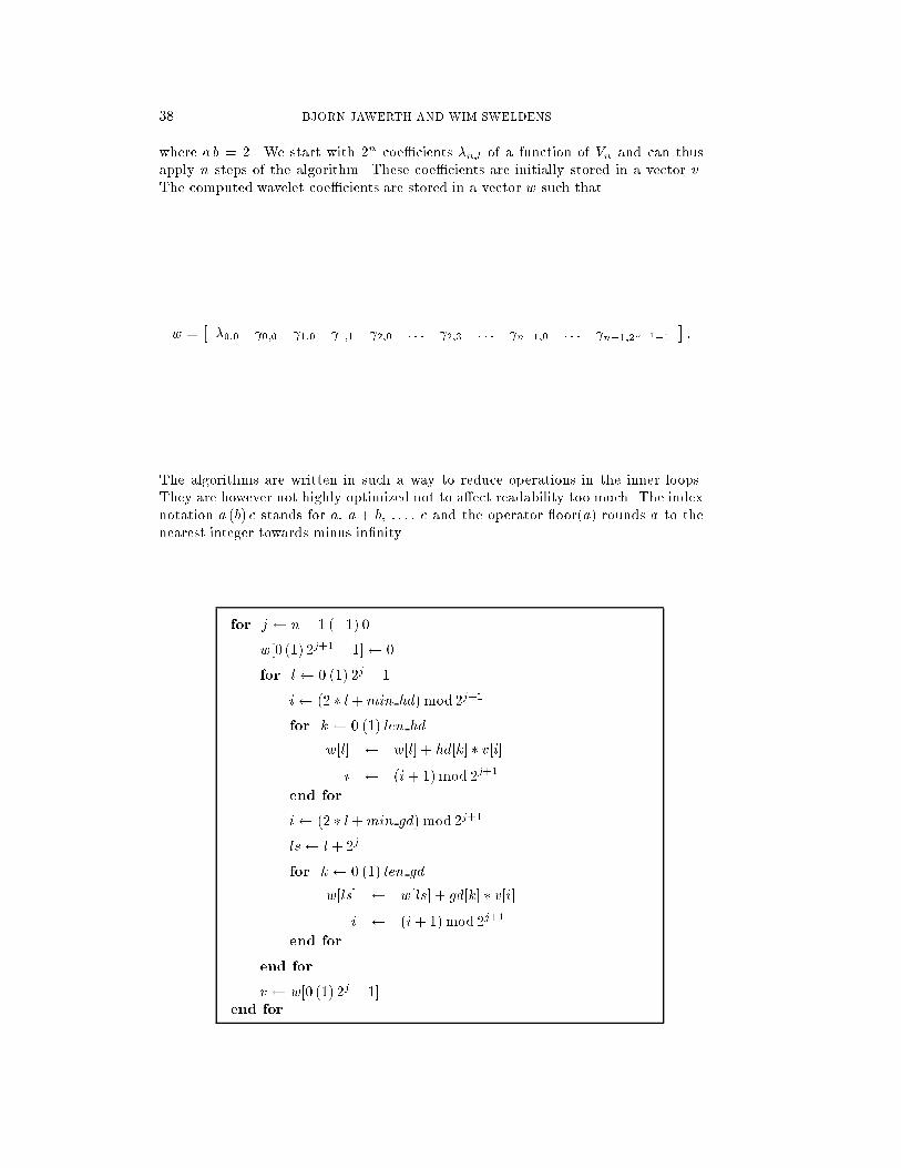
38 BJORN JAWERTH AND WIM SWELDENS
where a b = 2. We start with 2n coe�cients �n;l of a function of Vn and can thusapply n steps of the algorithm. These coe�cients are initially stored in a vector v.The computed wavelet coe�cients are stored in a vector w such that
w =��0;0 0;0 1;0 1;1 2;0 : : : 2;3 : : : n�1;0 : : : n�1;2n�1�1
�:
The algorithms are written in such a way to reduce operations in the inner loops.They are however not highly optimized not to a�ect readability too much. The indexnotation a (b) c stands for a, a + b, : : : , c and the operator oor(a) rounds a to thenearest integer towards minus in�nity.
for j n � 1 (�1) 0
w[0 (1) 2j+1 � 1] 0
for l 0 (1) 2j � 1
i (2 � l +min hd) mod 2j+1
for k 0 (1) len hd
w[l] w[l] + hd[k] � v[i]
i (i+ 1)mod 2j+1
end for
i (2 � l +min gd) mod 2j+1
ls l + 2j
for k 0 (1) len gd
w[ls] w[ls] + gd[k] � v[i]
i (i+ 1)mod 2j+1
end for
end for
v w[0 (1) 2j � 1]end for

AN OVERVIEW OF WAVELET BASED MULTIRESOLUTION ANALYSES 39
for j 1 (1) n
v[0 (1) 2j � 1] 0
for k 0 (1) 2j � 1
i ( oor((k�min hp)=2))mod 2j�1
lb (k �min hp) mod 2
for l lb (2) len hp
v[k] v[k] + hp[l] �w[i]
i (i� 1) mod 2j�1
end for
i ( oor((k�min gp)=2))mod 2j�1
lb (k �min gp) mod 2
for l lb (2) len gp
v[k] v[k] + gp[l] �w[i + 2j+1]
i (i� 1) mod 2j�1
end for
end for
w[0 (1) 2j � 1] = v
end for


![GENERAL EMPIRICAL BAYES AW VELET METHODS ...[j] are the Bayes rules when the priors are taken to be the unknown empirical distributions of {θk,k∈[j]}. Consider the estimation of](https://img.dokumen.tips/doc/110x75/60ef897c2953690e6f7bb96f/general-empirical-bayes-aw-velet-methods-j-are-the-bayes-rules-when-the-priors.jpg)

![Open Access Research articleComplete chloroplast genome ......(MP), implemented in PAUP* vers. 4.0b10 [17]. ML anal-yses were run under the general time reversible model, with all](https://img.dokumen.tips/doc/110x75/60ae0f5a9525d23ed35b5a60/open-access-research-articlecomplete-chloroplast-genome-mp-implemented.jpg)


![Simplifying Surfaces with Color and Texture using Quadric ..../garland/Papers/quadric2.pdfet al. [1] discussed adding surface color to a wavelet-based mul-tiresolution framework, andHugheset](https://img.dokumen.tips/doc/110x75/601911c64074d2664011c58b/simplifying-surfaces-with-color-and-texture-using-quadric-garlandpapers.jpg)


