Embed Size (px)
Citation preview

1
Ahmed Abdallah Abdou
AN INVESTIGATION OF SHORT RANGE
ELECTROMAGNETIC WAVE COMMUNICATION
FOR UNDERWATER ENVIRONMENTAL MONITORING
UTILISING A SENSOR NETWORK PLATFORM
AHMED ABDALLAH ABDOU
A THESIS SUBMITTED IN PARTIAL FULFILMENT OF THE
REQUIREMENTS OF LIVERPOOL JOHN MOORES UNIVERSITY
FOR THE DEGREE OF DOCTOR OF PHILOSOPHY
July 2014

2
Ahmed Abdallah Abdou
Acknowledgments
This research project would not have been possible without the support of my creator “ALLAH”
Glorious is He and He is exalted.
I wish to express my gratitude to my director of study, Dr A. Shaw for his invaluable support and
guidance. Deepest gratitude are also due to the members of the supervisory group Dr A. Mason
and Prof. A. Al-Shamma’a. I am grateful to Dr. J. Cullen for his abundant knowledge and
assistance. Special thanks to E. Hoare for her administrative support and to the entire RFM group
and to members of the Built Environment and Sustainable Technologies (BEST) Research
Institute. I am also thankful to Liverpool John Moores University for encouraging students by
making available scholarships or other means of financial assistance. I wish to express my love
and gratitude to my beloved parents for their endless love through the duration of my studies. My
thanks are also due to my whole family, family in law and all my friends. Deepest thanks to my
uncles for their support. I also wish to express my love and gratitude to my adored wife for her
understanding and the support, patience and endless love she offered to me.

3
Ahmed Abdallah Abdou
To the President of the Republic of Djibouti, the First Lady, all members of his
Government and the People of Djibouti, Yemen and Somalia
To my family Alrassouly & Almozati, my father and my mother, my brother and
sisters, my wife, my son Sajed, my daughter, my other children that will come and
grandchildren …

4
Ahmed Abdallah Abdou
Abstract
Current state of the art water communications systems rely on optical and acoustic propagation.
But these have underperformed in many applications. Wireless Sensor Network (WSN) using
radio communication underwater is state of the art. The frequency of operation and the antenna
are the big challenges that if unlocked, will present many advantages. The aim of this research is
to investigate short range electromagnetic wave communication for underwater environmental
monitoring utilising a sensor network platform. Theoretical study and preliminary experiments
have confirmed that ISM (industrial, scientific and medical) band at 433MHz was suitable for
potable and freshwater communication. Traditional antennas have been constructed, tested and
modelled in a High Frequency Simulator Structure (HFSS) but were found unsuitable for use
underwater. A 433MHz bowtie antenna was modelled in HFSS and shown to perform well in
both air and potable water without any matching circuit. The antenna was prototyped on a
printed circuit board, waterproofed and tested successfully in a tank. Furthermore to eliminate
RF crosstalk, a battery powered wireless transmitter that generated a carrier signal at 433MHz,
was used successfully in the laboratory tank, and during experiments that were repeated in
freshwater in Liverpool Stanley Canal. This range, in excess of 5m, was large enough to combine
the bowtie antenna with off the shelf, low power transceivers operating at the 433MHz, and
specific sensors to form a WSN for potable and freshwater applications. The contribution to
knowledge is the experimental demonstration of reliable communication at 433MHz using a
broadband antenna which unlocks the potential of underwater WSN applications, including
applications in water quality measurement, using radio communication.

5
Ahmed Abdallah Abdou
Contents
Chapter 1. Research background .............................................................................................. 23
1.1. Introduction .................................................................................................. 23
1.2. Properties of water ....................................................................................... 23
1.3. Impacts on water courses ............................................................................. 25
1.3.1. Water pollution types ............................................................................... 25
1.3.2. Causes and damage of water pollution .................................................... 28
1.4. Legislation ..................................................................................................... 30
1.5. Recent governmental engagement .............................................................. 34
1.6. Current monitoring methods ....................................................................... 37
1.6.1. Water sampling ......................................................................................... 37
1.6.2. Sensor technology ..................................................................................... 38
1.6.3. Real time technologies .............................................................................. 39
1.7. Design specification ...................................................................................... 40
1.8. Research aims and objectives....................................................................... 40
1.9. Thesis overview ............................................................................................ 41

6
Ahmed Abdallah Abdou
Chapter 2. Literature review of current state of the art water communication ...................... 44
2.1. Introduction .................................................................................................. 44
2.2. Underwater Wired Network technology ...................................................... 44
2.3. Underwater wireless communication point to point ................................... 46
2.3.1. Acoustic propagation ................................................................................ 46
2.3.2. Optical communication ............................................................................. 51
2.3.3. Electromagnetic (RF and Microwave) communication ............................ 56
2.4. Wireless Sensor Networks in water.............................................................. 58
2.4.1. Underwater WSN using Acoustic communication .................................... 59
2.4.2. Underwater WSN using Optical communication ...................................... 60
2.4.3. State of the art proposed system: Underwater WSN using Electromagnetic (RF and
Microwave) communication .................................................................................... 61
2.5. Summary ....................................................................................................... 64
Chapter 3. Electromagnetic (EM) wave propagation ............................................................... 65
3.1. Introduction .................................................................................................. 65
3.2. Maxwell equations ....................................................................................... 66
3.3. Electromagnetic waves propagation ............................................................ 67

7
Ahmed Abdallah Abdou
3.4. Electromagnetic spectrum ........................................................................... 70
3.5. Electromagnetic wave propagation underwater ......................................... 73
3.5.1. Permittivity of water ................................................................................. 73
3.5.2. Attenuation of EM wave propagation in water ........................................ 86
3.6. Experimental verification ............................................................................. 89
3.6.1. Underwater experiments using an off-the-shelf kit at 2.4GHz ISM ......... 89
3.6.2. Impact of the antenna and the frequency on the underwater communication
99
3.7. Summary ..................................................................................................... 103
Chapter 4. Traditional antennas and water ............................................................................ 105
4.1. Introduction ................................................................................................ 105
4.2. Antenna theory ........................................................................................... 105
4.3. Construction and tests of traditional antennas in water ........................... 107
4.3.1. Experiment .............................................................................................. 107
4.3.2. Results ..................................................................................................... 109
4.3.3. Discussion................................................................................................ 110
4.4. Modelling a traditional loop antenna ......................................................... 110

8
Ahmed Abdallah Abdou
4.4.1. Loop antenna modelling in water ........................................................... 111
4.4.2. Results and discussion for 12.3mm radius loop antenna modelled in water 114
4.4.3. Results and discussion for loop antenna radius 16mm modelled in water116
4.4.4. Results and discussion of the 12.3mm radius loop antenna modelled in Air 118
4.4.5. Results and discussion of loop antenna modelled from wavelength calculation in
air 121
4.5. Summary ..................................................................................................... 123
Chapter 5. Bow-tie antenna.................................................................................................... 124
5.1. Introduction ................................................................................................ 124
5.2. Antenna selection and background ............................................................ 124
5.3. Modelling the Bow-tie antenna in air and in water ................................... 127
5.3.1. Design and simulations ........................................................................... 127
5.3.2. Results and discussion ............................................................................ 131
5.4. Construction of the antenna ...................................................................... 135
5.4.1. EAGLE PCB design software .................................................................... 136
5.4.2. CNC routing machine .............................................................................. 137
5.5. Waterproofing the PCB antenna for s11 tests ........................................... 139

9
Ahmed Abdallah Abdou
5.6. Experimental setup of bow-tie antenna’s S11 in air and in water ............. 140
5.7. Experiment results in air and in water for S11 ........................................... 141
5.8. Discussion ................................................................................................... 143
5.9. Further experimental investigation on the bow-tie antenna: the temperature change
effects in water ......................................................................................................... 144
5.9.1. Experiment setup .................................................................................... 144
5.9.2. Results and discussion ............................................................................ 145
5.10. Summary ..................................................................................................... 148
Chapter 6. Wireless transmitter ............................................................................................. 150
6.1. Introduction ................................................................................................ 150
6.2. Electronics................................................................................................... 150
6.3. Waterproofing the wireless transmitter .................................................... 154
6.4. Experimental setup for S21 with off-the-shelve PP containers in laboratory156
6.4.1. Transmission in air and in water at vertical separation.......................... 156
6.4.2. Radiation pattern in air and in water at vertical separation .................. 157
6.4.3. Radiation pattern in water at horizontal separation .............................. 158
6.5. Results for a S21 experiment with off-the-shelve PP containers in laboratory159

10
Ahmed Abdallah Abdou
6.5.1. Transmission at vertical separation distances in air and in water ......... 159
6.5.2. Radiation pattern in air and in water at vertical separation .................. 160
6.5.3. Radiation pattern in water at horizontal separation .............................. 162
6.5.4. Comparing bowtie radiation pattern in water at vertical and horizontal separation
163
6.6. Summary ..................................................................................................... 165
Chapter 7. Real world tests in Liverpool Stanley canal .......................................................... 166
7.1. Introduction ................................................................................................ 166
7.2. Design and prototyping of a waterproof PVC enclosure ............................ 166
7.2.1. Transmitter’s enclosure .......................................................................... 166
7.2.2. Receiver’s enclosure ............................................................................... 173
7.3. Effect of the fabricated PVC enclosure on the transmission ...................... 174
7.4. Experimental method for S11 and S21 with the fabricated PVC enclosures in the
canal 175
7.4.1. S11 Reflection coefficient for Smith Chart ............................................. 179
7.4.2. S11 Return loss ........................................................................................ 179
7.4.3. S21 Transmission at horizontal separation ............................................. 180

11
Ahmed Abdallah Abdou
7.4.4. S21 Radiation pattern at horizontal separation ..................................... 181
7.5. Results and discussion ................................................................................ 182
7.5.1. S11 Reflection coefficient in Smith chart ................................................ 182
7.5.2. Return Loss .............................................................................................. 184
7.5.3. S21 Transmission at horizontal separation ............................................. 185
7.5.4. S21 Radiation pattern at horizontal separation in Stanley canal ........... 186
7.6. Summary ..................................................................................................... 188
Chapter 8. Further Modelling with the Bowtie antenna ........................................................ 190
8.1. Introduction ................................................................................................ 190
8.2. Case 1: restricted to an antenna board of 210mm length and 120mm width191
8.2.1. Bowtie antenna design alteration and modelling .................................. 191
8.2.2. Results and discussion ............................................................................ 192
8.3. Case 2: not restricted to the levelling board length, arm length size could be
increased ................................................................................................................... 194
8.3.1. Bowtie antenna design optimisation and modelling .............................. 194
8.3.2. Results and discussion ............................................................................ 195
8.4. Summary ..................................................................................................... 197
12
Ahmed Abdallah Abdou
Chapter 9. Conclusion ............................................................................................................. 198
Chapter 10. Future work ....................................................................................................... 205
References .................................................................................................................................. 207
List of figures:
Figure 1 Common sources of pollution [5] ................................................................................... 26
Figure 2 Underwater wired sensor network ................................................................................. 45
Figure 3 Underwater acoustic communication ............................................................................ 46
Figure 4 Commercial acoustic transducer or hydrophone [39] .................................................... 47
Figure 5 Array of hydrophones towed from a ship to pick up sounds in the water and help locate
the animals that are producing the sounds [40] .......................................................................... 47
Figure 6 Absorption coefficient, [dB/km] [42].......................................................................... 49
Figure 7 The transmitter and receiver of AquaOptical [50] ......................................................... 52
Figure 8 Neptune Underwater Communications with laser communication getting tested in San
Diego Harbour [52] ....................................................................................................................... 53
Figure 9 Underwater radio S1510 transmitter and receiver [64] ................................................. 57
Figure 10 Underwater radio modem Seatooth S200 [64] ............................................................ 58

13
Ahmed Abdallah Abdou
Figure 11 Underwater radio modem Seatooth S300 [64] ............................................................ 58
Figure 12 Underwater multi hop Wireless Sensor Network ......................................................... 63
Figure 13 Main sensor node hardware components.................................................................... 64
Figure 14 Source-free electric and magnetic fields [79] ............................................................... 68
Figure 15 Transverse electromagnetic (TEM) wave ..................................................................... 69
Figure 16 Electromagnetic spectrum [80] .................................................................................... 70
Figure 17 Frequency band regions allocated by ITU [81] ............................................................. 72
Figure 18 Permittivity of water with S=0ppt referred to as distilled water at T=20⁰C................. 77
Figure 19 Permittivity of water with S=0.0871ppt referred to as potable water T=20⁰C ............ 78
Figure 20 Permittivity of water with S=0.335 referred to as freshwater canal at T=20⁰C ........... 78
Figure 21 Permittivity of water with S=20ppt referred to as seawater at T=20⁰C ....................... 79
Figure 22 Effect of temperature on the real and imaginary parts of the permittivity of water
with salinity concentration S=0ppt referred to as distilled water ................................................ 81
Figure 23 Effect of temperature on the real and imaginary parts of the permittivity of water
with salinity concentration S=0.0871ppt referred to as potable water ....................................... 82
Figure 24 Effect of temperature on the real and imaginary parts of the permittivity of water
with salinity concentration S=0.335ppt referred to as canal freshwater ..................................... 83

14
Ahmed Abdallah Abdou
Figure 25 Effect of temperature on the real and imaginary parts of the permittivity of water
with salinity concentration S=20ppt referred to as seawater ...................................................... 84
Figure 26 Attenuation (dB/m) in water with different concentrations of salinity S, in relation to
the operating frequency (Hz) ........................................................................................................ 88
Figure 27 eZ430RF2500 Wireless sensor kit ................................................................................. 90
Figure 28 Experimental setup of sensors in containers on table in air ........................................ 91
Figure 29 Experimental setup of sensors in containers in a small tank with potable water ....... 91
Figure 30 Data for sensors in air ................................................................................................... 92
Figure 31 Temperature sensor monitor in air .............................................................................. 92
Figure 32 Data for sensors in water .............................................................................................. 93
Figure 33 Temperature sensor monitor in water ......................................................................... 93
Figure 34 RSSI (dBm) of eZ430RF2500 Wireless sensor kit in air and in potable water at 100mm
separation distance compared to datasheet values .................................................................... 94
Figure 35 Experimental setup of sensors in containers in a big tank with potable water ........... 96
Figure 36 Signal amplitude of eZ430RF2500 (2.4GHz) sensors in air and in water ...................... 97
Figure 37 Signal amplitude of eZ430RF2500 (2.4GHz) sensors in water at 20mm increments ... 97
Figure 38 Double loop antennas of 320mm diameter with their frames .................................. 100

15
Ahmed Abdallah Abdou
Figure 39 Experimental setup at ISM frequencies with double loop antennas ......................... 100
Figure 40 Comparison of chip antennas and double loop antennas at 2.4 GHz underwater .... 101
Figure 41 Signal amplitude at ISM frequencies up to 1000mm with 320mm double loop antenna
..................................................................................................................................................... 101
Figure 42 Losses in cables (1m, 2.4m and 11m) at ISM frequencies .......................................... 102
Figure 43 Antennas built for experiments (from right to left: one wavelength monopole with
ground, a half wavelength monopole, one wavelength loop and one wavelength dipole ........ 108
Figure 44 Experimental setup of built antennas......................................................................... 109
Figure 45 Signal amplitude for different type and size of antennas at ISM 433MHz frequency for
varying distances up to 1m ......................................................................................................... 109
Figure 46 Ansoft HFSS window, panels and 3Dmodel of designed 12.3mm radius loop antenna
..................................................................................................................................................... 112
Figure 47 Side-view of the designed 12.3mm radius loop antenna within a radiation boundary
..................................................................................................................................................... 113
Figure 48 Return loss of the 12.3mm radius loop antenna simulated in water ......................... 114
Figure 49 Smith chart of the impedance of the 12.3mm radius loop antenna simulated in water
..................................................................................................................................................... 115

16
Ahmed Abdallah Abdou
Figure 50 3D radiation plot of the gain of the 12.3mm radius loop antenna simulated in water
..................................................................................................................................................... 115
Figure 51 3D radiation field of the 12.3mm radius loop antenna simulated in water with respect
to its position .............................................................................................................................. 115
Figure 52 Return loss of the 16mm radius loop antenna simulated in water ............................ 117
Figure 53 Smith chart of the impedance of the 16mm radius loop antenna simulated in water
..................................................................................................................................................... 117
Figure 54 3D radiation plot of the gain of the 16mm radius loop antenna simulated in water 118
Figure 55 3D radiation field of the 16mm radius loop antenna simulated in water with respect
to its position .............................................................................................................................. 118
Figure 56 Return loss of the 12.3mm radius loop antenna simulated in air .............................. 119
Figure 57 Smith chart of the impedance of the 12.3mm radius loop antenna simulated in air 119
Figure 58 3D radiation plot of the gain of the 12.3mm radius loop antenna simulated in air .. 120
Figure 59 3D radiation field of the 12.3mm radius loop antenna simulated in air with respect to
its position ................................................................................................................................... 120
Figure 60 Return loss of the 117mm radius loop antenna simulated in air ............................... 121
Figure 61 Smith chart of the impedance of the 117mm radius loop antenna simulated in air . 122

17
Ahmed Abdallah Abdou
Figure 62 Diagrams of a Biconical and a Bow-tie antenna with flare angle α, cone diameter or
outer width D, plate length L ...................................................................................................... 126
Figure 63 Screen shot of the Bowtie antenna created in HFSS’s ADK and its parameters for the
433MHz desired operating frequency ........................................................................................ 128
Figure 64 Modelling of the 433MHz bow-tie antenna within a radiation box in HFSS .............. 130
Figure 65 Return loss of the simulated 433MHz Bow-tie antenna in air ................................... 131
Figure 66 Return loss of the simulated 433MHz Bow-tie antenna in water .............................. 132
Figure 67 Smith Chart of the Input impedance for the simulated Bow-tie antenna in air ........ 133
Figure 68 Smith Chart of the Input impedance for the simulated Bow-tie antenna in water ... 133
Figure 69 3D radiation pattern of the simulated Bow-tie antenna in air ................................... 134
Figure 70 3D radiation pattern of the simulated Bow-tie antenna in water .............................. 135
Figure 71 PCB layout of the Bow-tie antenna in EAGLE software .............................................. 136
Figure 72 CNC Routing machine connected to a PC in the LJMU Sensors laboratory ................ 137
Figure 73 HPGL format of the Bow-tie antenna in ABViewer7 software ................................... 138
Figure 74 CCD-control software RoutePro 2000 ........................................................................ 138
Figure 75 Angle view of the Bow-tie antenna fabricated with the CNC Routing machine ........ 139
Figure 76 PCB Bow-tie antenna waterproofed with glue with its isolated RF cable .................. 140

18
Ahmed Abdallah Abdou
Figure 77 Experiment setup for S11 Return Loss in water ......................................................... 141
Figure 78 S11 Experimental results in air of the constructed Bow-tie antenna ......................... 142
Figure 79 S11 Experimental results in water of the constructed Bow-tie antenna ................... 142
Figure 80 Simulated and experimented S11 (dB) of a bow-tie antenna in air and in water ...... 143
Figure 81 Experimental setup for temperature change effects on the antenna ....................... 145
Figure 82 S11 return loss data of the antenna at different temperatures in water .................. 145
Figure 83 Smith chart of S11 reflected coefficient Г real and imaginary data of the antenna in
water at different temperatures within the 400-500MHz region .............................................. 147
Figure 84 S11 return loss at 433MHz of the antenna at different temperatures in water ........ 148
Figure 85 Carrier signal creation using DC power supply ........................................................... 151
Figure 86 Block diagram of the transmitter’s carrier generator ................................................ 152
Figure 87 Battery powered transmitter’s carrier generator set ................................................. 153
Figure 88 433MHz carrier signal test on spectrum analyser ...................................................... 154
Figure 89 Opened up polypropylene waterproof set ................................................................. 155
Figure 90 Closed up polypropylene waterproof set ................................................................... 155
Figure 91 Experimental setup for S21 transmission in air .......................................................... 156
Figure 92 Experimental setup for S21 transmission in water ..................................................... 157

19
Ahmed Abdallah Abdou
Figure 93 Experimental setup for radiation pattern at horizontal separation ........................... 159
Figure 94 Comparison of bowtie antenna’s signal strength (S21) experimented in air and in
water over distance up to 450mm ............................................................................................. 160
Figure 95 Comparison of bowtie antenna’s signal strength radiation pattern (S21) over radiation
angles in air and in water at a vertical separation of 100mm .................................................... 161
Figure 96 Comparison of bowtie antenna’s signal strength radiation (S21) over radiation angles
in air and in water at a vertical separation of 500mm ............................................................... 162
Figure 97 Comparison of bowtie antenna’s signal strength radiation (S21) over radiation angles
in water at horizontal separation of 500mm and 1000mm ....................................................... 163
Figure 98 Comparison of bowtie antenna’s signal strength radiation (S21) over radiation angles
in water at horizontal and vertical separation of 500mm .......................................................... 164
Figure 99 Exploded view of transmitter’s enclosure designed in SolidWorks ........................... 167
Figure 100 PVC cover .................................................................................................................. 168
Figure 101 PMMA ....................................................................................................................... 169
Figure 102 PVC Cover .................................................................................................................. 169
Figure 103 Cylinder ..................................................................................................................... 170
Figure 104 O Ring for cylinder .................................................................................................... 170
Figure 105 PVC cylinder Bottom cover ....................................................................................... 171

20
Ahmed Abdallah Abdou
Figure 106 Transmitter’s enclosure ............................................................................................ 172
Figure 107 Underwater transmitter ........................................................................................... 172
Figure 108 Receiver’s enclosure designed in SolidWorks........................................................... 173
Figure 109 Underwater receiver ................................................................................................. 173
Figure 110 Effects of the fabricated PVC enclosure on the transmission .................................. 174
Figure 111 Bing maps, top view of the Stanley canal locks and their surroundings [116]
(in circle: Top Lock Footbridge)................................................................................................... 175
Figure 112 Anritsu MS2711D Handheld Spectrum Analyser ...................................................... 176
Figure 113 R&S ZVL Vector Network Analyser 9kHz to 3GHz ..................................................... 177
Figure 114 Halfords portable powerpack 200 ............................................................................ 177
Figure 115 Other equipment used for the canal experiments ................................................... 178
Figure 116 S11 of receiver in Stanley Top Lock (Lock No 1) Footbridge .................................... 179
Figure 117 S21 Horizontal test for signal strength of transceivers against distance in Stanley Top
Lock (Lock No 1) Footbridge ....................................................................................................... 180
Figure 118 Floats attached to transmitter and receiver in air in laboratory .............................. 181
Figure 119 Floats attached to submerged transmitter and receiver in the canal ...................... 181
Figure 120 S21 Radiation pattern experiment at horizontal separation in Stanley canal ......... 182

21
Ahmed Abdallah Abdou
Figure 121 Smith chart for the receiver’s antenna in Stanley canal for frequencies 400-
500MHz ....................................................................................................................................... 183
Figure 122 S11 Return loss of the receiver’s antenna in Stanley canal ...................................... 184
Figure 123 S21 Transmission of transceivers separated horizontally in the canal water .......... 185
Figure 124 S21 radiation pattern (up to approximately 90˚) at horizontal separation in Stanley
canal ............................................................................................................................................ 187
Figure 125 S21 Radiation pattern and predicted at horizontal separation in Stanley canal ...... 188
Figure 126 Schematic of Bowtie antenna with reduced arm length from 101.6mm to 20mm on a
210mm×120mm antenna board ................................................................................................. 191
Figure 127 Return Loss (dB) of the Bowtie antenna modelled in water with reduced arm length
from 101.6mm to 20mm ............................................................................................................ 192
Figure 128 Schematic of Bowtie antenna with increased arm length from 101.6mm to 160mm
on a 350×120mm antenna board ............................................................................................... 194
Figure 129 Return Loss (dB) of the Bowtie antenna modelled in water with increased arm length
from 101.6mm to 160mm .......................................................................................................... 195
List of tables:
Table 1 Radio and microwave frequency bands allocated for Industrial Scientific and Medical
(ISM) applications by the International Telecommunication Union (ITU) ................................... 71

22
Ahmed Abdallah Abdou
Table 2 Real and Imaginary parts of permittivity at ISM frequencies .......................................... 85
Table 3 Attenuations of ISM operating frequencies in water with different salinity concentration
....................................................................................................................................................... 87
Table 4 Real parts permittivity, reduction factor , velocity v (m/s) in water, wavelength in
water and in air (mm) for ISM frequencies (Hz) ......................................................................... 107
Table 5 New dimensions of the bowtie antenna ....................................................................... 129
Table 6 Measured dimensions in HFSS of the Bowtie with reduced arm length from 101.6mm to
20mm .......................................................................................................................................... 192
Table 7 Consequences of reduced arm length from 101.6mm to 20mm of the Bowtie antenna
modelled in water ....................................................................................................................... 193
Table 8 Measured dimensions in HFSS of the Bowtie antenna with increased arm length from
101.6mm to 160mm ................................................................................................................... 195
Table 9 Consequences of increased arm length from 101.6mm to 180mm of the Bowtie antenna
modelled in water ....................................................................................................................... 196

Chapter 1 Research background
23
Ahmed Abdallah Abdou
Chapter 1. Research background
1.1. Introduction
People need water to survive. It is important that communities, industry, agriculture and the
environment get a sustained supply of high quality water. Water pollution occurs from
different sources and increases with population. The severity of the damage pushes
international communities and national authorities to enforce laws and regulations.
Environmental agencies and industry currently apply traditional methods for assessing water’s
health.
1.2. Properties of water
In water, there are many important properties to be taken into account. A change in these
parameters may indicate a change in the quality of the water. These parameters include
temperature, pH, conductivity, turbidity, dissolved oxygen and suspended solids.
Temperature exerts a major influence on biological activity and growth. Temperature
governs the kinds of organisms that can live in rivers and lakes. Water temperature can
affect the ability of water to hold oxygen as well as the ability of organisms to resist
certain pollutants. It is also important because of its influence on water chemistry.
Portable water thermometers include thermocouples and infrared.
pH is a measure of how acidic or alkaline water is. The range goes from 0 to 14, with 7
being neutral. When pH is less than 7 it indicates acidity, whereas a pH of greater than
7 indicates a base. pH is a measure of the relative amount of free hydrogen and

Chapter 1 Research background
24
Ahmed Abdallah Abdou
hydroxyl ions in the water. Water that has more free hydrogen ions is acidic, whereas
water that has more free hydroxyl ions is basic. Pollution can change water's pH, which
in turn can harm animals and plants living in the water. There are large model pH
metres for use in labs and small portable models for field use. An estimate of pH can
be given by using Litmus paper which is a strip of paper with colour change indicating
a rough estimation.
Conductivity is a measure of the ability to conduct an electrical current. It is highly
dependent on the amount of dissolved solids (such as salt) in the water. In seawater,
conductivity is ≈4S/m [1] whereas for freshwater it is 100 times lower ≈0.05S/m [2].
Measured with a conductivity meter, the specific conductance is an important water-
quality measurement because it gives a reliable indication of the amount of dissolved
material in the water. Total Dissolved Solids (TDS) metres measure the quantity of
solids in water in parts per thousands (ppt). It has been discovered experimentally that
there is an approximate relationship between conductivity and TDS [3]. The
conversion from S/m to ppt can be done by multiplying by 5 in water with a high
proportion of sodium chloride and by a factor of 6.7 for most other waters. Therefore,
the TDS of a 4S/m conductive seawater can be calculated as 20ppt whereas for
0.05S/m conductive freshwater is 0.335ppt.
Turbidity is a measure of suspended matter in water. High concentrations of particulate
matter affect light penetration and habitat quality. In streams, increased sedimentation
and siltation can occur, which can result in harm to habitat areas for fish and other
aquatic life. Particles also provide attachment places for other pollutants, notably
metals and bacteria. For this reason, turbidity readings can be used as an indicator of
potential pollution in a water body. Turbidity is measured in nephelometric turbidity
units (NTU) with a turbidity sensor by shining a light into the water and reading how
much light is reflected back to the sensor.

Chapter 1 Research background
25
Ahmed Abdallah Abdou
Suspended solids are solids whose sizes exceed 1mm. These include sand, silt, rust,
plant fibres and algae. They are an indicator of possible bacterial or hazardous
contamination. Total suspended solids are the mass of solids that can be separated from
the water by filtration.
Dissolved Oxygen (DO) refers to the volume of oxygen present in water and it is a
basic indicator of ecosystem health. A small amount of oxygen, up to about ten
molecules of oxygen per million of water, is dissolved in water. This dissolved oxygen
is breathed by fish and zooplankton and is needed by them to survive. Bacteria in water
can consume oxygen as organic matter decays. Thus, excess of organic material in
lakes and rivers can cause eutrophic conditions, which is an oxygen-deficient situation
that can cause a water body “to die”. DO can be measured using electrodes
(electrochemical sensors) and optodes (optical sensors).
1.3. Impacts on water courses
One of the main concerns with water is the quality and refers to the pollution of water. Water
pollution is the contamination of natural water bodies by chemical, physical, radioactive or
pathogenic microbial substances. Water pollution affects drinking water, rivers, lakes and
oceans all over the world. This consequently harms human health and the natural environment.
1.3.1. Water pollution types
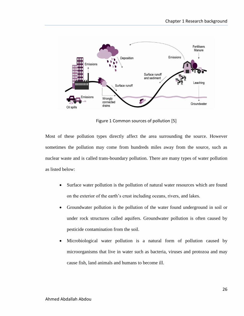
Water pollution can come from a number of different sources as displayed in Figure 1. Point
source and nonpoint source pollution can be distinguished [4]. The former refers to pollution
coming from a single source such as an oil spill. The second refers to pollution coming from
many sources such as agricultural runoff.
Chapter 1 Research background
26
Ahmed Abdallah Abdou
Figure 1 Common sources of pollution [5]
Most of these pollution types directly affect the area surrounding the source. However
sometimes the pollution may come from hundreds miles away from the source, such as
nuclear waste and is called trans-boundary pollution. There are many types of water pollution
as listed below:
Surface water pollution is the pollution of natural water resources which are found
on the exterior of the earth’s crust including oceans, rivers, and lakes.
Groundwater pollution is the pollution of the water found underground in soil or
under rock structures called aquifers. Groundwater pollution is often caused by
pesticide contamination from the soil.
Microbiological water pollution is a natural form of pollution caused by
microorganisms that live in water such as bacteria, viruses and protozoa and may
cause fish, land animals and humans to become ill.
Chapter 1 Research background
27
Ahmed Abdallah Abdou
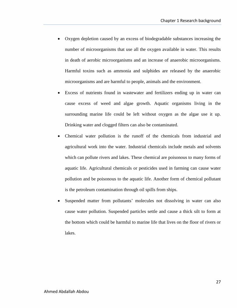
Oxygen depletion caused by an excess of biodegradable substances increasing the
number of microorganisms that use all the oxygen available in water. This results
in death of aerobic microorganisms and an increase of anaerobic microorganisms.
Harmful toxins such as ammonia and sulphides are released by the anaerobic
microorganisms and are harmful to people, animals and the environment.
Excess of nutrients found in wastewater and fertilizers ending up in water can
cause excess of weed and algae growth. Aquatic organisms living in the
surrounding marine life could be left without oxygen as the algae use it up.
Drinking water and clogged filters can also be contaminated.
Chemical water pollution is the runoff of the chemicals from industrial and
agricultural work into the water. Industrial chemicals include metals and solvents
which can pollute rivers and lakes. These chemical are poisonous to many forms of
aquatic life. Agricultural chemicals or pesticides used in farming can cause water
pollution and be poisonous to the aquatic life. Another form of chemical pollutant
is the petroleum contamination through oil spills from ships.
Suspended matter from pollutants’ molecules not dissolving in water can also
cause water pollution. Suspended particles settle and cause a thick silt to form at
the bottom which could be harmful to marine life that lives on the floor of rivers or
lakes.

Chapter 1 Research background
28
Ahmed Abdallah Abdou
1.3.2. Causes and damage of water pollution
The causes of water pollution are multiple and their consequences are harmful to humans and
animals. Damage could be immediate or after long term exposure. The causes and
consequences of water pollution include:
Sewage and wastewater produced by domestics households, industrial and
agricultural practices can cause pollution of lakes and rivers. Sewage in developed
countries is carried away from the home quickly and hygienically through sewage
pipes. However if chemicals and pharmaceutical substances are flushed down the
toilet, sewage can cause problems. When people are ill; sewage often carries
harmful viruses and bacteria into the environment causing health problems. In
developing countries sewage disposal is a major problem and untreated sewage
water can contaminate the environment and cause diarrhoea or typhoid which are
the primary cause of infant mortality.
Industrial water pollution is when industry produces pollutants that are harmful to
people and the environment, as many industrial facilities use freshwater to carry
away waste from the plant and into rivers, lakes and oceans. These pollutants could
be asbestos, lead mercury, nitrates, phosphates, sulphur, oil and petrochemicals.
Some of these pollutants may have a mild effect; others can be serious and may
result in immune suppression, reproductive failure or acute poisoning.
Oil pollution can be caused by oil spills, routine shipping, run-offs and dumping in
oceans. Although an oil spill may be a localised problem, it has severe effects on

Chapter 1 Research background
29
Ahmed Abdallah Abdou
the local marine wildlife such as fish, birds and sea otters. As oil cannot dissolve in
water, it forms a thick mud which suffocates fish and stops birds from flying as it
gets caught on their feathers. It also blocks light from photosynthetic aquatic
plants.
Atmospheric deposition is the pollution caused by air pollution. When it rains,
droplets are polluted with gases such as carbon dioxide, sulphur dioxide and
nitrogen oxide forming acid rain. Acid rain pollutes, and may harm, rivers, lakes
and aquatic life.
Dumping of litter in aquatic environments causes problems. For example a six pack
ring packaging can trap marine animals and may cause their death. Different items
take different time to degrade in water. Cardboard can take 2 weeks to degrade
whereas foam and plastic packaging may take up to 50 and 400 years respectively.
Nuclear waste can be produced in industrial, medical and scientific processes that
use radioactive material. Mining and refining of uranium and thorium can form
marine nuclear waste. Nuclear waste has damaging effects and is harmful to marine
habitats
Leakages of petroleum into the surrounding soil and groundwater from old
underground steel storage tanks which have corroded over time. This
contamination can affect drinking water and cause health problems.
Global warming increasing water temperature can disrupt many marine habitats
and result in the death of many aquatic organisms. Coral reef bleaching is an
example of water temperature rise making the coral reef expels the microorganisms

Chapter 1 Research background
30
Ahmed Abdallah Abdou
on which it is dependent. Other corals may be contaminated and this may affect the
marine life that depends on them.
Eutrophication refers to when the environment is supplemented with nutrients that
may cause problems such as algal blooms in marine environment. The excess of
nutrients may come from nearby farming water run-off containing fertilizers. This
causes rapid growth of phytoplankton resulting in algal bloom. Other than
depleting the oxygen in the water, algae may also block sunlight from
photosynthetic underwater plants.
1.4. Legislation
There are many laws that protect the world’s oceans, rivers, lakes and ground water
from unnecessary water pollution. Each continent and country may differ in which laws they
enforce but they aim to have the same overall positive influence.
At the international level, legislation regarding water pollution focuses more on marine
pollution but also regulates transboundary watercourses and international lakes.
A number of conventions were signed at an international level to prohibit dumping of
waste and other hazardous materials at sea. These date back to 1954 with the
International Convention for the Prevention of Pollution of the Sea by Oil [6]. Along
with others, these laws have been enforced to regulate oil spillages from ships and
other vessels.

Chapter 1 Research background
31
Ahmed Abdallah Abdou
Other international laws deals with transboundary watercourses and international lakes
like the Convention on the Protection and use of Transboundary Watercourses and
International Lakes 1992 [7] and their amendments.
The European Community set out water pollution as a priority matter at its first action
programme on the environment in 1973. Since then, a number of European directives have
been introduced to reduce and control pollution in European waters. There are also lots of
European laws to control and prevent pollution of rivers, lakes, ground waters, estuaries and
coastal areas and include:
The urban waste water directive which aims to protect surface inland waters and
coastal waters from pollution by regulating the collection and treatment of urban waste
water. [8]
The nitrate from agricultural sources directive which aims to protect waters against
pollution caused by nitrates especially from agricultural sources such as fertilisers.
This will enable marine and freshwaters to be protected from eutrophication. [9]
The drinking water directive which aims to establish strict standards regarding the
quality of drinking water. The directive provides parameters and analysis methods;
these standards must be met to ensure safe drinking water. [10]
The Water Framework Directive WFD (2000/60/EC) within the European Community,
which became part of the United Kingdom law in 2003, came into force to protect and
enhance the quality of surface freshwater (including lakes, streams and rivers),
groundwater, estuaries, coastal waters [11]. The overall objectives of the WFD are to

Chapter 1 Research background
32
Ahmed Abdallah Abdou
provide a sufficient supply of good quality surface and ground water to provide for
sustainable, balanced and equitable water use throughout the member states. Also to
significantly reduce pollution in both ground and surface waters that has continued to
show an overall reduction in quality over the past decades even though legislation has
been put in place to protect them. Finally to protect the marine environment by
reducing the concentration of pollutants to near background values for naturally
occurring substances and to zero for man-made synthetic substances [12].
The Environmental Liability Directive 2004/35/EC establishes a framework based on
“the polluter pays” principle to prevent and remedy environmental damage [13]. This
applies to marine pollution incidents like oil spills if they damage protected habitats or
species, or coastal waters.
The bathing water directive aims to keep good standards in the quality of bathing water
in freshwater and coastal water areas [14].
The Marine Strategy Framework Directive 2008/56/EC aims to achieve good
environmental status in Europe’s seas by 2020. It requires member states to assess the
state of their seas, set standards and introduce a programme of measures for achieving
good environmental status [15].
In England and Wales, a range of national laws consolidate existing water pollution laws and
others implement the international and European laws. Some of the laws are listed below and
aim to:

Chapter 1 Research background
33
Ahmed Abdallah Abdou
Consolidate existing laws to regulate water quality and prevent pollution of water in
the Water Resources Act 1991. This has been amended in 2009 as in [16].
Consolidate existing laws related to regulation of water and sewerage industries in the
Water Industry Act 1991 [17].
Implement the European environment liability directive in England and Wales. These
national 2009 SI 2009/153 and SI 2009/995 regulations respectively for England and
Wales refer to the environmental damage (Prevention and Remediation) and hold the
operator responsible; in the case of imminent threat of environmental damage or actual
environmental damage the operator is to take immediate steps to prevent damage or
further damage and to notify the authority [18].
Introduce a new framework for managing the demands placed on the sea, improving
marine conservation and opening up access for the public to the English coast as stated
in the marine and coastal access act 2009 [19].
Implement the European marine strategy regulations under 2010, SI 2010/1627
regulation for the achievements of good environmental status seas.
Implement the European water quality standards
Give effect to the European water framework directive in the water environment
regulation focusing to achieve good chemical and ecological status of inland and
coastal waters by 2015.
Authorities are required to set and achieve certain water quality standards. The Environment
Agency in England and Wales has taken the lead to carry out a set of approaches and meet
certain goals in order to contribute to the future of water health with regards to the Water

Chapter 1 Research background
34
Ahmed Abdallah Abdou
Framework Directive WFD (2000/60/EC). To achieve this directive, the Environment Agency
has responsibilities cited in [20] including:
Analysing the characteristics of the 11 River Basin Districts in England and Wales
and assessing the impact of human activity on the water bodies within these
districts.
Monitoring the status of water bodies against the objectives set for them.
Preparing, reviewing and keeping an up to date register of protected areas for each
River Basin District.
Preparing and consulting on the River Basin Management Plans Taking the lead in
drawing up and carrying out Program of Measures.
In each River Basin District in England and Wales, liaison panels made up of individuals from
water companies, ports, business and industry, the Consumer Council for Water, agriculture,
other industry sectors specific to the district and environmental regulators, have been created.
1.5. Recent governmental engagement
The Natural Choice White Paper published in June 2011 in [21] on the Natural Environment
emphasizes the importance of valuing nature and the benefits it offers. The paper
acknowledges that rivers, lakes, groundwater, estuaries, wetlands and river corridors provide
vital ecosystem services and public benefit. But only 27% of river and lakes are fully
functioning ecosystems. Under EU law, England is legally required to improve this figure by
2017. The department is keen to change water bodies in England to be in excellent health, with
reduced pollution (nutrients, sediments, chemical and bacteria) by 2050. Along the way, the

Chapter 1 Research background
35
Ahmed Abdallah Abdou
aim is to increase the proportion of water bodies in Good Ecological Status (GES) from 26%
to 32% by 2015, then get the majority of bodies to GES as soon as possible and get as many of
the water bodies as possible to GES by 2027.
The U.K. government is also committed to achieve good environmental status across
England’s marine area, working in partnership with those who use, enjoy and derive their
income from the marine environment. The Government has set the strategic policy framework
through the UK Marine Policy Statement, adopted in March 2011.
In December 2011, another White Paper named Water for Life was published in [22] by the
Department for Environment Food and Rural Affairs (DEFRA). This makes clear that damage
done to water ecosystems has to be stopped and reversed, so they can continue to provide
essential services to people and the natural environment. It is cited that damage to rivers and
other water bodies comes from pollution and over abstraction. They acknowledge an
improvement in tackling pollution classified as point sources pollution such as discharges
from sewage treatment works and industrial processes. However tackling diffuse pollution
coming from many pollution sources such as run-off from roads and farmland, and detergents
and other toxic materials people put down drains, is still a problem.
A strategy to identify and address the most significant diffuse sources of water pollution from
non-agricultural sources is projected. The government is committed to protect water
ecosystems to achieve good ecological status through a river basin planning approach under
the EU Water Framework Directive.

Chapter 1 Research background
36
Ahmed Abdallah Abdou
A consultation ran from November 2012 to February 2013 to inform and influence
development of the strategy for the management on urban diffuse water pollution in England
and a report was published in [23] by DEFRA.
Through a series of questions to be answered, views were sought to tackle the problem. A
summary of the answers to the consultation is published in [24].
The actions undertaken by the government to improve water quality are cited in [25] and
include:
Planning for better water: the government is working with partners across the U.K.
to plan for better water quality and protect sensitive local areas such as bathing
water.
Managing catchments: ten catchment-level partnerships are established to develop
and implement plans for creating and maintaining healthy water bodies.
Reducing agricultural pollution: the government is working closely with farmers to
reduce pollution from farms affecting rivers and water bodies.
Controlling urban pollution: the government is working closely with the
Environment Agency to understand urban pollution better, as sources may be
numerous.
Controlling chemical pollution: chemical pollutants are monitored and reduced in
open water and other water bodies to protect the environment.
Managing waste water, sludge and septic tanks: working to make sure pollutants
from waste water, sludge and septic tanks are reduced and controlled.

Chapter 1 Research background
37
Ahmed Abdallah Abdou
A Public Policy Exchange symposium will be held in London in September 2014 to give
opportunity for local authorities, central government including non-departmental public
bodies, water companies, businesses, the environmental sector, regulators, civil society
groups, third sector organisations and other key stakeholders to discuss how we can help to
protect and improve water quality for ourselves and generations to come.
However to meet European and international standards, the Government, Environment
Agency, water companies and other partners are currently relying on periodic and single point
measurement methods to monitor water bodies.
1.6. Current monitoring methods
1.6.1. Water sampling
The revised European Community Directive [26] that relates to the quality of water for human
consumption adopted at the end of 1998, has required new water quality regulations to be
drawn in the United Kingdom. Regulations and developments in sampling and analytical
techniques required revision. This has resulted in a series of booklets being published under
the name The Microbiology of Drinking Water, and provides general advice and guidance on
many microbiological aspects connected with potable water supplies, as well as giving details
of methods. In the first part [27] of the booklet named Methods for the Examination of Waters
and Associated Materials, which contains details of the practices and procedures that should
be adopted for taking samples for microbiological analysis, it is stated that the results of a
laboratory examination of any single water sample are representative only of the water at the
time and at that particular point at which the sample is taken. Furthermore satisfactory results

Chapter 1 Research background
38
Ahmed Abdallah Abdou
from single samples do not justify an assumption that the water is safe to drink at all times and
that contamination is often irregular and may not be revealed by the examination of a single
sample. In the second part [28] it is reported that whenever a sample is taken for analysis it
should be recognised, irrespective of the volume of water sampled, this volume represents
only a very small fraction of the water being sampled. Along with the sampling procedures
come other important requisitions for sample handling techniques, preservation and
transportation of the samples. Furthermore, if fluctuations occur then accuracy of the sampling
reduces and the only way of increasing sampling accuracy is by increasing the sampling
frequency which will incur further cost.
1.6.2. Sensor technology
Traditional water sampling procedures incur a high cost in engaging a full cycle of separate
actions from preparing the procedure, trough collecting, storing and analysing the samples
present many disadvantages. An alternative for this standard water sampling procedure is to
use sensor technologies. A sensor is used for an element which produces a signal relating to
the quantity being measured. Sensors can be analogue or digital depending on the nature of
their outputs. A sensor is said to be analogue if its output can change over a continuous range
to represent the measured parameter. If the sensor gives outputs which are digital in nature, i.e.
a sequence of on/off signals which can be interpreted as a number whose value is related to the
size of the variable being measured, the sensor is called digital. Handheld water quality
sensors are available to purchase in [29] and [30] for single parameter or multi-parameter
monitoring. Such units are sometimes called probes and their price can go up to £1000 for a
dissolved oxygen sensor [31]. Other than the high cost of these probes, the geographical

Chapter 1 Research background
39
Ahmed Abdallah Abdou
monitoring area is limited to the probe (single point measurement) and the readings are stored
in-situ for manual periodic retrieval.
1.6.3. Real time technologies
Real time technologies involve sending the data sampled automatically by adding telemetry to
the monitoring sensor system. Such systems will allow fast responses and actions. These
systems are integrated in floating buoys and are commercialised in [32]. One of these modules
has been used to monitor the water quality in the Dubai creek, UAE [33]. The buoy is moored
to a heavy anchor and is able to take readings from the multi-parameter sensor to monitor
temperature, pH, salinity, dissolved oxygen concentration and Chlorophyll A. The buoy is
equipped with a cell phone modem which communicates readings to the base station computer
in Dubai municipality. Another application using floating buoy system was installed in 2000
in Wales’ Cardiff Bay [34]. The system was then upgraded in 2008 to automatically publish
live data to a dedicated website. The cost of these systems and their maintenance is high and
they do not provide geographical coverage.
Although the challenges in water environment are becoming more alarming, industrial and
environmental bodies have kept relying on traditional in-situ and periodic methods in
assessing water health. As technology is evolving, it is providing solutions to many problems.
Only some of environmental agencies and water industries in developed countries have made
use of technology with the revolution of sensors technology and real time systems. In
countries with financial resource shortage, the cost of these systems makes it almost
impossible to acquire them. Therefore globally there has been a huge need for scientists and

Chapter 1 Research background
40
Ahmed Abdallah Abdou
technologists to find new and cheap alternatives capable of replacing conventional and costly
ways for assessing water environment in real time.
1.7. Design specification
If a WSN requires a large number of nodes, then the overall cost can be minimised by using
off-the-shelf transceivers. Commercial transceivers are only available in the ISM bands. To
design an underwater WSN for water quality monitoring using electromagnetic propagation in
one of the ISM bands requires the following:
A range of at least 3 metres.
A sufficient bandwidth to convey all the sensor data from a large number of distributed
nodes, as well as overheads such as handshaking and encryption. It is envisioned that
256kbps would be sufficient data rate that would also provide some necessary
redundancy.
The antennas need to be insensitive to possible changes in the permittivity of water, of
a manageable size and cheap to manufacture. With this in mind it was decided to limit
the maximum antenna dimension to 250mm.
As the sensors are liable to move in flowing water, the orientation of the antennas
cannot be guaranteed; therefore an omnidirectional antenna will be used.
To maximise battery lifetime, the transmitted power will be limited to +6dBm.
1.8. Research aims and objectives
To achieve the aim of this research, several objectives have to be met which include:
Investigate the feasibility of RF underwater communications using the unlicensed ISM
bands
Chapter 1 Research background
41
Ahmed Abdallah Abdou
Test the feasibility of using commercially over air wireless transceivers in water
Design, simulate and test an antenna to operate efficiently underwater
Investigate the feasibility of forming a wireless sensor network to operate in water.
1.9. Thesis overview
In order to achieve the aim and meet the objectives of this research, the thesis is structured in
chapters. The first chapter has discussed the importance of water, the problems faced in many
water environments and the current methods used to assess water’s health.
In the second chapter, a literature review will describe and evaluate state of the art
technologies used underwater. This will lead to highlighting a need to investigate
electromagnetic (radio and microwave) communication underwater utilising a sensor network
platform.
In chapter 3, the theory of electromagnetic wave propagation in air and in water will be
studied thoroughly and verified with preliminary experiments. This will predict the behaviour
of the electromagnetic wave in water so that a useful frequency band is located within the
spectrum.
In Chapter 4, as antennas are another crucial element in underwater radio and microwave
communication along with frequency of operation, a set of traditional antennas will be
investigated. These antennas will be made for the 433MHz ISM band and tested in water. Also
a modelling stage in High Frequency Structure Simulator will permit to predict and analyse
the behaviour of the antennas with regards to the change of medium (air and water). A study

Chapter 1 Research background
42
Ahmed Abdallah Abdou
on antenna parameters will lead to assessing the suitability of using traditional narrowband
antennas in underwater communication systems.
In chapter 5, a technique of using a broadband antenna will be revealed and applied to
accommodate change of properties in air designed antenna when used in water. A potential
broadband Bowtie antenna will be modelled in air then in water using HFSS to validate the
technique. The antenna will be designed on Easily Applicable Graphical Layout Editor
(EAGLE) which will then be loaded on the computer numerical control routing machine to
produce the antenna on a printed circuit board. The antenna will be tested in air and in a tank
with potable water and the return loss results will be then compared to the results of the
modelling.
Chapter 6 will involve the setup of a complete wire free transmitter. A setup consisting of
batteries powered electronics will generate a carrier signal operating in the ISM band at
433MHz. The electronics and the batteries of the transmitter will be waterproofed to undergo
underwater tests. In the laboratory, the carrier signal will be transmitted in air and its strength
will be measured by the receiver which consists of another waterproofed antenna connected to
a spectrum analyser. Then the experiment will be repeated in potable water in a tank. A
comparison for air and water will be given. Other tests will include the antenna’s radiation
pattern in air and in water.
In chapter 7, the transceivers will be subjected to real world applications. Therefore a robust
plastic container will be designed in SolidWorks and prototyped to house the electronics, the
batteries and the antennas. The tests will take place in the freshwater Stanley canal in

Chapter 1 Research background
43
Ahmed Abdallah Abdou
Liverpool, United Kingdom. Tests will include reflection coefficient, horizontal transmission
and radiation pattern.
In chapter 8, further modelling of the Bowtie antenna in water will be done to see if the
antenna can be optimised by changing its dimension. Two cases will be presented. The first
case will be the reality that we are restricted on the size of the antenna board because of the
PCB levelling board. The second case is that the length of the board could be increased. The
available bandwidth and the lower frequency will be monitored in each case.

Chapter 2 Literature review of current state of the art water communication
44
Ahmed Abdallah Abdou
Chapter 2. Literature review of current state of the art water
communication
2.1. Introduction
Underwater communication is of great interest to military, industry and scientific
communities. This growing interest has extended the range of underwater applications and has
pushed researchers to find new and cheap alternatives. To reduce cost, provide geographical
coverage and offer real time information for taking reactive remedial action as appropriate,
sensors must be able to communicate even while submerged. Investigation on the current state
of the art water communication technologies shows a diversity of techniques is used. These
include underwater wired networks, wireless point to point communications and wireless
sensor networks with the last two using acoustic and optical propagation commonly. Each of
these has its advantages and disadvantages. However the growing fast application ranges in
water along with the development of WSN technology and their availability in markets at low
prices have recently triggered interest of the use of WSN in water.
2.2. Underwater Wired Network technology
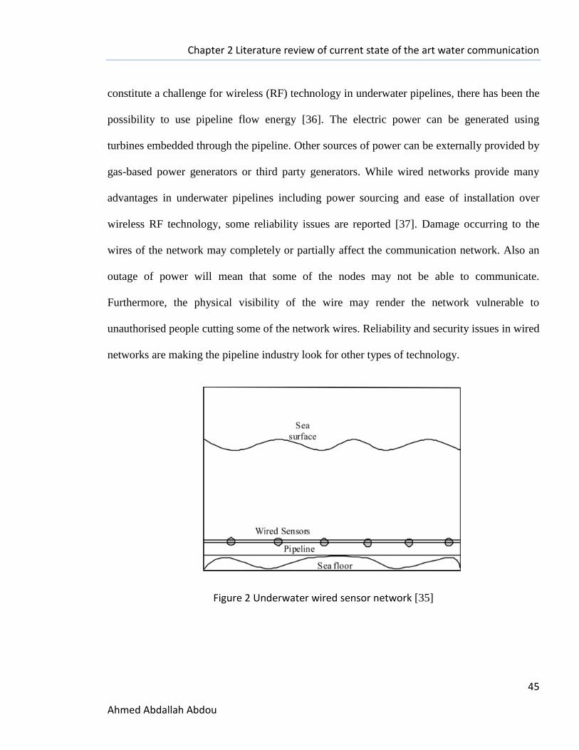
Wired Networks have been used underwater to monitor pipelines as explained in [35]. The
wired network allows measurement of many sensors including vibration, temperature, flow
rate, pressure in the vicinity of the pipes as in Figure 2. These sensors are electrically powered
by the wired network which also serves as their communication link. While power may
Chapter 2 Literature review of current state of the art water communication
45
Ahmed Abdallah Abdou
constitute a challenge for wireless (RF) technology in underwater pipelines, there has been the
possibility to use pipeline flow energy [36]. The electric power can be generated using
turbines embedded through the pipeline. Other sources of power can be externally provided by
gas-based power generators or third party generators. While wired networks provide many
advantages in underwater pipelines including power sourcing and ease of installation over
wireless RF technology, some reliability issues are reported [37]. Damage occurring to the
wires of the network may completely or partially affect the communication network. Also an
outage of power will mean that some of the nodes may not be able to communicate.
Furthermore, the physical visibility of the wire may render the network vulnerable to
unauthorised people cutting some of the network wires. Reliability and security issues in wired
networks are making the pipeline industry look for other types of technology.
Figure 2 Underwater wired sensor network [35]

Chapter 2 Literature review of current state of the art water communication
46
Ahmed Abdallah Abdou
2.3. Underwater wireless communication point to point
Underwater communication systems have been used in a broad range of applications including
submarine and surface vessels, coastal surveillance, real-time control of unmanned underwater
vehicles (UUV), diver to diver communication, automated underwater vehicles (AUV), oil and
gas exploration and environmental research etc. There are three main types of communications
systems and these use acoustic, optical or electromagnetic (radio & microwave) propagation.
2.3.1. Acoustic propagation
Underwater acoustic communication is a technique of sending and receiving messages below
water [38]. There are several ways of employing such communication but the most common is
using hydrophones or acoustic transducers as in Figure 3.
Figure 3 Underwater acoustic communication [40]
A hydrophone is a microphone designed to be used underwater for recording or listening to
underwater sound. A commercial hydrophone is displayed in Figure 4. Most hydrophones are
based on a piezoelectric transducer that generates electricity when subjected to a pressure
change. Such piezoelectric materials or transducers can convert a sound signal into an

Chapter 2 Literature review of current state of the art water communication
47
Ahmed Abdallah Abdou
electrical signal or vice versa since sound is a pressure wave. Multiple hydrophones can be
arranged in an array like in Figure 5 so that it will add the signals from the desired direction
while subtracting signals from other directions.
Figure 4 Commercial acoustic
transducer or hydrophone [39]
Figure 5 Array of hydrophones towed from a ship
to pick up sounds in the water and help locate the
animals that are producing the sounds [40]
Acoustic monitoring is also used to determine whether or not a sound source is affecting the
behaviour of marine animals [40]. For example, dolphins and beluga whales have been found
to shift the frequency of their clicks to avoid noise in the normal frequency range of their
echolocation [41]. This indicates that noise may be affecting the animals by reducing the
efficiency of their echolocation.

Chapter 2 Literature review of current state of the art water communication
48
Ahmed Abdallah Abdou
2.3.1.1. Attenuation of acoustic waves
Attenuation, or path loss that occurs in an underwater acoustic channel over a distance for a
signal of frequency is defined in [42] by:
( ) ( )
(1)
Where is a unit-normalising constant, is the spreading factor, and ( )is the absorption
coefficient. The acoustic path loss is expressed in dB by:
( )
( )
(2)
The first term in the above summation represents the spreading loss and the second term
represents the absorption loss. The spreading factor k describes the geometry of propagation
which are for spherical spreading, for cylindrical spreading and for the
so-called practical spreading. The absorption coefficient can be expressed empirically, using
the Thorp’s formula which gives ( ) in dB/km for in kHz as in [43] by:
( )
(3)
This formula is generally valid for frequencies above a few hundred Hz. For lower
frequencies, the following formula may be used:

Chapter 2 Literature review of current state of the art water communication
49
Ahmed Abdallah Abdou
( )
(4)
The absorption coefficient is displayed in Figure 6. It increases rapidly with frequency, thus
imposing a limit on the maximum usable frequency for an acoustic link of a given distance.
For a 1MHz signal, the absorption coefficient is approximately 320dB/km compared to a 100
kHz signal with 40dB/km of absorption coefficient.
Figure 6 Absorption coefficient, ( )[dB/km] [42]
The path loss represents the attenuation on a single unobstructed propagation path. If a signal
of frequency and power is transmitted over this path then the received signal power is

Chapter 2 Literature review of current state of the art water communication
50
Ahmed Abdallah Abdou
( ). When there are multiple propagation paths, each of length , , the
channel transfer function is described by:
( ) ∑ √ ( )
(5)
where is the distance between the transmitter and receiver, represents the additional
losses incurred on the th path (e.g. reflection loss), and is the delay with
c=1500m/s defined as the nominal speed of sound underwater.
2.3.1.2. Noise
Another important factor in an underwater channel with acoustic propagation is the noise. In
the ocean, the ambient noise can be modelled using four sources: turbulence, shipping, waves
and thermal noise. Details of the empirical formula are given in [44] and it models the four
noise components by their power spectral density (p.s.d). The overall p.s.d of the ambient
noise is the sum of all four noise components and an approximation is given as follows:
( )
(6)
In the plot of the empirical model and the approximation of ambient noise p.s.d in [42], one
can see that noise level is high at low frequencies then decays at the higher end of the acoustic
spectrum.

Chapter 2 Literature review of current state of the art water communication
51
Ahmed Abdallah Abdou
Recalling that the acoustic path loss is frequency dependent, it then imposes a bandwidth
limitation on the underwater communication system, such that a greater bandwidth is available
for a shorter transmission distance. This has pushed underwater point to point acoustic
researchers towards a network of acoustic modems.
Although many underwater communication systems prefer acoustic as a method of underwater
wireless transmission, they present some disadvantages. Underwater acoustics suffer from low
velocity; the operating frequencies limit the bandwidth and therefore the data rate is reduced.
In deep water, acoustic signals only propagate well with very low frequency signal carriers,
which reduce the signal bandwidth and transmission rates, thus extending communication
time, which shortens battery life. In shallow water underwater acoustic attenuation is
unfeasibly high [45]. Underwater acoustics suffer from multipath propagation and poor
performance due to turbidity and ambient noise and has a negative impact on the marine life
[46].
2.3.2. Optical communication
Underwater optical communication is a technique for transmitting and receiving light in a
water medium. Underwater optical communication has been studied by other research groups
in the past. The traditional way was to use Infrared communication (IR) as in [47] where an
underwater analogue communication system was reported. It uses infrared light to transmit
crayfish neuronal activity information from live crayfish in a small aquarium of 30cm width ×
40cm depth × 15cm height. The maximum distance at which the transmitted signal could be
received was tested in a larger aquarium and found to be 50 cm. Then the use of visible light

Chapter 2 Literature review of current state of the art water communication
52
Ahmed Abdallah Abdou
generated by Light Emitting Diodes (LEDs) and Lasers became popular considering the
minimum absorption wavelength window of the water [48]. LED based systems are the most
common types of underwater optical systems because they have been demonstrated for low-
cost, low-power, and compact systems [49]. With the aim of surveying underwater habitats,
optical communication systems were developed in [50]. The AquaOptical system depicted in
Figure 7 is claimed to achieve a data rate of 1.2Mbit/sec at distances up to 30m in clear water.
In water with visibility estimated at 3m, it claims achieving communication at data rates of
0.6Mbit/sec at distances up to 9m. Although these are considered to be low cost, turbidity has
a big influence on its reliability.
Figure 7 The transmitter and receiver of AquaOptical [50]
However laser-based systems have been demonstrated for extended ranges, high data rates and
low latencies [51]. The Neptune Underwater Communications displayed in Figure 8 from

Chapter 2 Literature review of current state of the art water communication
53
Ahmed Abdallah Abdou
Saphotonics is a commercial product consisting of a flexible laser transmitter. Its modulation
capability is based on water conditions and link distance. They claim a data rate up to 250
Mbps at distances up to 200 metres, depending on water turbidity. However if that is to be
used in a low visibility water or in the case of disturbed sediment at seabed, this would make
the laser fail to operate.
Figure 8 Neptune Underwater Communications with laser communication getting tested in
San Diego Harbour [52]
For high speed optical communication, waveguide modulated optical lasers have been
proposed in [53]. They demonstrated optical communication at 1Gbit/s through a short
distance of 2m. The device is however directional, very bulky and expensive due to the
difficulty in modulating green lasers at high speed.

Chapter 2 Literature review of current state of the art water communication
54
Ahmed Abdallah Abdou
2.3.2.1. Attenuation of optical waves
In optical communication, the two major causes of attenuation of light are absorption and
scattering. Absorption refers to the conversion of the electromagnetic energy into another form
of energy such as heat or chemical. Scattering is when the electromagnetic radiation is
redirected away from its original path. These two processes are wavelength dependant and are
represented by:
( ) ( ) ( )
(7)
Where a and b are absorption and scattering measured in m-1
, and is the vacuum wavelength
of light, in nm.
The attenuation of an optical signal for a distance d is formulated in Beer’s law using the
attenuation coefficient as:
( )
(8)
With regards to attenuation coefficient variation with wavelength and chlorophyll
concentration, it is reported [54] that the ideal wavelength of a vertical optical wireless
communication link for each of the profiles represented by varying surface chlorophyll
concentration, is extremely dependent on the expected length of the link, especially in places
of high surface chlorophyll. Therefore the selection of an appropriate wavelength for a
communication system depends significantly on the expected orientation and location of the
link. This may limit the use of the underwater communication system to specific applications.

Chapter 2 Literature review of current state of the art water communication
55
Ahmed Abdallah Abdou
The refractive index of the ocean water also changes with depth and potentially can lead to a
long distance communication link being diverged away from the receiver.
Simulation work carried out in Matlab and published in [55] shows the effects of four types of
water including pure sea water, clean ocean water, coastal ocean water and turbid harbour
water on the underwater optical wireless communication system with a wavelength of 405nm
and 650nm for a distance of 10m. In the scattering results both wavelengths have similar high
scattering behaviour in the turbid water. Furthermore, the total attenuation results demonstrate
higher attenuation levels on both wavelengths for turbid water compared to the rest which
present a lower attenuation level.
2.3.2.2. Noise
In free space optical communication devices, background optical noise is a limitation [56].
Sources of noise include solar light, sunlight reflected by the moon at night which can be a
problem in shallow water, and also artificial light sources. In underwater at depth up to 10
metres, the main source of noise is solar light [57].
Optical communications underwater have the potential to achieve much higher data transfer
rates than an acoustic communication system at significantly lower power consumption,
simpler computational complexity, and smaller packaging, unfortunately its use is limited due
to turbidity and environmental background noise, conditions that vary widely across different
oceans and other bodies of water [58]. Other drawbacks of optical communication include
optical scattering caused by suspended particles and planktons, high levels of ambient light in

Chapter 2 Literature review of current state of the art water communication
56
Ahmed Abdallah Abdou
the upper part of the water column, multipath propagation and beam spreading, drive
researchers to look for alternative technologies.
2.3.3. Electromagnetic (RF and Microwave) communication
Radio and Microwave propagation underwater is a good alternative in situations where
traditional acoustic and optical communications fail to operate. This includes congested and
noisy underwater environments like ports and harbours, in shallow water and in water with a
high turbidity level. With a high speed of propagation up to around , EM
propagation offers many advantages including propagation velocity, bandwidth, data rate and
better transmission in crossing boundaries (air, water, seabed and ice). EM wave propagation
is clearly faster than acoustic and this has important advantages for command latency and
networking protocols where signals get exchanged between nodes and sinks. It is perfect for
noisy environments where acoustic signals will be highly affected. Furthermore as far as we
know it has no effects on marine life whereas acoustic is becoming an issue for marine
mammals.
Research on electromagnetic propagation underwater has been going on since the World War І
for US navy submarines in the extreme low frequency range [59]. This work on seawater has
been followed by many others who have significantly contributed. Besides, research and
experiments conducted in Liverpool John Moores University have claimed that transmission
of 5MHz frequency is feasible in seawater up to 90m at a high data rate of 500kbps that allows
duplex video and data streams [60]. In [61], propagation at frequencies of 6 MHz and
10.7MHz in a reflective metal tank were possible. Recently a review [62] on EM propagation

Chapter 2 Literature review of current state of the art water communication
57
Ahmed Abdallah Abdou
underwater has been conducted and predicted its usefulness in wireless communication at high
frequencies for high data rates which could be used in many applications. Furthermore, the
authors carry out an experimental study in potable water with off-the-shelf transceivers
operating at 2.4GHz Industrial Scientific and Medical (ISM) band, resulting in a successful
communication range of 200mm [63]. To increase the range they suggested that the lower
ISM frequency 433MHz could be used and a different antenna that is specially designed for
water communication should be sought.
Leading from theoretical and experimental seawater investigations published in [1] and in
[60], Wireless For Subsea is one of the companies that currently sell wireless RF underwater
systems [64]. They claimed in 2006 that underwater radio modem S1510 (Figure 9) transmits
up to 3 metres in seawater with 0.6W of power at 40bps data rate. They also claim that
Seatooth S200 (Figure 10) transmits up to 30 metres through seawater at 16W of power.
However the data rate is 100bps due to the low frequency of operation. Their latest claim
includes Seatooth S300 (Figure 11) transmitting up to 7 metres in seawater at a data rate of
156kbps. Although the power transmitted is high and the antennas used are conventional loops
that require matching, there is no published evidence which support their claims.
Figure 9 Underwater radio S1510 transmitter and receiver [64]

Chapter 2 Literature review of current state of the art water communication
58
Ahmed Abdallah Abdou
Figure 10 Underwater radio modem Seatooth S200 [64]
Figure 11 Underwater radio modem Seatooth S300 [64]
2.4. Wireless Sensor Networks in water
In the past decade, production of sensor nodes has soared due to the demand of different
sensor nodes applications. These include large power hungry devices from Sensoria e.g. the
Sensoria WINS NG 2.0 [65], which are used when power is not an issue, as well as the System
on Chip (SoC) classified devices referred to as “motes”. Motes are designed to be both small
and low power. There are many families of motes including μAmp, BT node, Firefly and
Berkeley’s range of Mica motes. Each of them has its own characteristics and aims.

Chapter 2 Literature review of current state of the art water communication
59
Ahmed Abdallah Abdou
In Liverpool John Moores University, researchers have been working on WSN applications
including spot welding monitoring in the automotive industry and asset tracking in the airline
and gas industry [66]. They have also used WSN in an environmental application for
monitoring car exhaust pollution [67]. Other WSN researchers have mainly focused on how to
make motes smaller, cheaper and lower powered. A few have tried to use WSN in unusual
places for EM propagation such as soil properties in underground monitoring [68]. The fast
growing application range in water along with the development of WSN technology and its
availability in markets have recently triggered interest of the use of WSN in water.
2.4.1. Underwater WSN using Acoustic communication
A miniature acoustic communication subsystem for underwater wireless sensor networks
called CORAL has been prototyped using a low power modem [69]. The system is tested in a
tank and 200mm of communication range is achieved with a transducer operating at 1.7 kHz.
This operating frequency limits the data rate. In water the bandwidth reported of 3.8 kHz is
relatively small and therefore limits the usefulness of the modem.
In [70], the design and implementation of an omni-directional underwater acoustic micro-
modem based on a low power micro-controller. The system is tested in a tank, pond and river.
The modem has been able to transmit wirelessly up to 70m with a data rate of 0.2kbps in the
river. The data rate is more than a thousand times less than can be achieved with a 256kbps
radio transceiver. This is due to the low frequency used which is one of the main drawbacks of
acoustic communication. Most importantly, the 4.5W energy used to power the system is not
compatible with the low power requirement in Wireless Sensor Networks.

Chapter 2 Literature review of current state of the art water communication
60
Ahmed Abdallah Abdou
2.4.2. Underwater WSN using Optical communication
A network is built around twenty underwater sensor nodes called Aquaflecks, for data
collection by an autonomous underwater vehicle [71]. Each node has a custom board for
optical communications that drives a high power LED and a sensitive matched photodiode.
The LED emits light in a 30 degree cone and supports a maximum data rate of 320kbits/s at a
maximum range of 2m. Although the transmission rate is high, the nodes need to be within the
30degree cone range for hard docking to allow short range communication in low turbidity
water environment. To overcome these challenges, the authors integrate acoustic
communication to cover a longer range of 20 metres with a low data rate of 50 bits/s.
Additional research on underwater wireless sensor networks based on optical communication
between two nodes is described in [72]. Challenges and results are also presented in the paper.
During the experimental tests in a tank, a transmission over 1.8 metres was achieved at 100
Kbps. However beyond 1.9 metres the bit error rate increased and made the transmission
impossible although the tests were performed in water with high visibility. Optical systems
were found to be impractical in high turbidity. Optical signals suffer from optical scattering
and are rapidly absorbed in water. Also the level of ambient light in the upper part of the water
is another adverse factor in using optical communication.
In [73] an underwater optical link is proposed for communication between sensors on a
swimmer during a training session. The system uses LED and an optical detector at 520nm.
The effects of bubbles are studied and experimented in a still pool, still spa water and bubble
spa water. The authors conclude that the path is still thought to be viable in the context of a

Chapter 2 Literature review of current state of the art water communication
61
Ahmed Abdallah Abdou
sensor network for swimmers for distances greater than 1 metre. As the relative movement
between the arm and the head is very large, the beamwidth of the transmitter and receiver
must be very large. The swimmer is located at the water–air interface. This can provide an
additional problem associated with changing ambient noise and changing surface reflection
conditions. During free-style swimming, the side of the goggles closest to the extended arm
with the wrist sensor is commonly in the water when the wrist is in air and vice versa. Also
one of objectives of the sensors is to communicate and collaborate as a network platform to
send information to the coach at poolside to provide direct feedback to the swimmer. For this
reason, a communications system that functions in both air and water is highly desirable.
Furthermore the high level of ambient light in the upper part of the water column and
multipath propagation would not make optical communication a viable solution.
2.4.3. State of the art proposed system: Underwater WSN using
Electromagnetic (RF and Microwave) communication
There are very limited trials of Wireless Sensor Networks in water using radio and microwave
propagation [74]. However, recently some groups including ourselves have shown interest in
investigating this technology. In [75], the authors publish their simulation work at 2.4GHz
ISM frequency band. The simulations are only run in air and the results are used to discuss as
if it was water. No evidence of simulations in water is presented. Moreover, the 2.4GHz is a
highly attenuated band in water and tests performed in published paper [63] achieved reliable
small communication range up to 200mm.

Chapter 2 Literature review of current state of the art water communication
62
Ahmed Abdallah Abdou
Additional research is based on the 2.4GHz ISM band [76]. The tests are performed with
transceivers and conventional antennas, and the maximum achieved communication range is
170mm. Both transceivers are connected to a laptop located outside the water via a serial
cable. The experimental setup used to make their measurements increases chances of signal
spreading out of the water through the cables. Furthermore, the separation distance is small
and does not seem feasible to build a wireless sensor network for geographical coverage.
2.4.3.1. Research overview
Current state of the art wireless sensor nodes rely on optical and acoustic propagation in water.
However these have underperformed in many applications. Radio and microwave
propagations underwater have many advantages but the communication range is affected by
the attenuation due to the conductivity and polar nature of water. However, of the ISM bands,
433MHz offers equilibrium between attenuation and data rate. As wireless nodes using
electromagnetic (radio and microwave) communication became cheaper and smaller, it
becomes viable to set a network of many nodes operating at 433MHz ISM band to cover a
large area. The nodes could organise themselves into a wireless sensor network, reconfigure
routes as radio link quality changes and cooperate in routing data packets to a base station
(multi-hop communication) as demonstrated in Figure 12. The sensor network deployed
underwater could monitor physical variables such as water temperature and pressure as well as
variables such as conductivity, turbidity and certain pollutants. The network could track
release of pollutants flowing into water from land. It could monitor and model the behaviour
of underwater ecosystems. The network could be used to identify or monitor in real time
deliberate pollution or even potential terrorist attack to water reservoirs that could contaminate

Chapter 2 Literature review of current state of the art water communication
63
Ahmed Abdallah Abdou
water supply and endanger public health. A map of the water reservoir with areas of
contamination could be generated for the authorities to take immediate action like stopping the
supply of contaminated water from getting to the public.
Figure 12 Underwater multi hop Wireless Sensor Network
The sensor node could comprise five components as in [77]: controller, memory, sensors and
actuators, communication device and power supply. The controller will process all the relevant
data, and is capable of executing codes. The memory will store programs and intermediate
data and usually different types of memory are used for programs and data. The sensors and
actuators are the actual interface to the physical world; these devices can observe or control
physical parameters of the water environment. The communication device allows nodes to
send and receive information over a wireless channel. The power supply, usually in the form
of batteries, is necessary to provide energy. All of these are shown in Figure 13.

Chapter 2 Literature review of current state of the art water communication
64
Ahmed Abdallah Abdou
Figure 13 Main sensor node hardware components [77]
2.5. Summary
State of the art water communication has been investigated. To provide geographical coverage
and reduce cost, a breakthrough in underwater communication is to use a wireless sensor
network. In many applications, acoustic and optical traditional ways of communicating
underwater between sensors nodes have underperformed and have been found unreliable. This
has triggered interest in alternatives including the underwater WSN using the radio and
microwave communication we are proposing. Therefore, electromagnetic propagation is
studied in the next chapter to understand the subject and to investigate a useful technology in
many underwater applications where acoustic and optical would fail to operate.

Chapter 3 Electromagnetic (EM) wave propagation
65
Ahmed Abdallah Abdou
Chapter 3. Electromagnetic (EM) wave propagation
3.1. Introduction
In this chapter the theory of electromagnetic wave propagation in air and in water will be
studied and compared with experimental results. At first, the important work of James
Maxwell’s equations which have been verified in optics, microwaves, antennas,
communications, radar and many sensing applications, in unifying the existing laws of
electricity and magnetism of the previous great scientists onto the well-known Maxwell model
will be explained. This will lead onto an elaboration on how an electromagnetic wave
propagates. An overview of the electromagnetic spectrum will be given, to show how it is
typically divided into frequency bands. This includes the radio and microwave band that the
Industrial Scientific and Medical band is part of. Then the theory of electromagnetic wave
propagation underwater will be revised. For this the permittivity of water will be thoroughly
studied, along with the effects of permittivity and salinity of water. Then a modification of the
attenuation model will be presented to take into account the losses due to the polar nature of
water. This will predict the behaviour of the electromagnetic wave in water to locate
theoretically a useful frequency band to communicate at. A set of experiments will follow
using an off the shelf transceiver operating at 2.4GHz ISM to verify the theory and to show the
capability of this frequency in water. Finally the impact of the antenna on the underwater
communication will be experimented on.
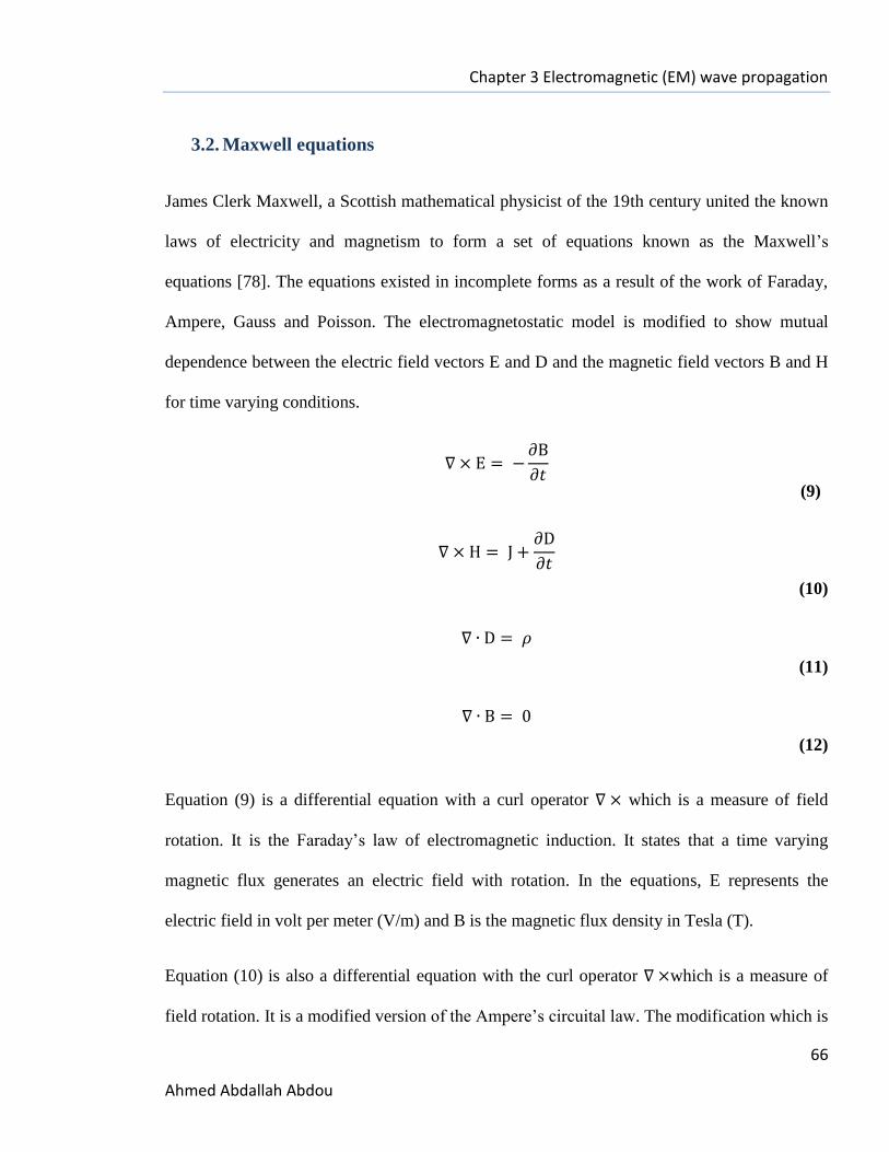
Chapter 3 Electromagnetic (EM) wave propagation
66
Ahmed Abdallah Abdou
3.2. Maxwell equations
James Clerk Maxwell, a Scottish mathematical physicist of the 19th century united the known
laws of electricity and magnetism to form a set of equations known as the Maxwell’s
equations [78]. The equations existed in incomplete forms as a result of the work of Faraday,
Ampere, Gauss and Poisson. The electromagnetostatic model is modified to show mutual
dependence between the electric field vectors E and D and the magnetic field vectors B and H
for time varying conditions.
(9)
(10)
(11)
(12)
Equation (9) is a differential equation with a curl operator which is a measure of field
rotation. It is the Faraday’s law of electromagnetic induction. It states that a time varying
magnetic flux generates an electric field with rotation. In the equations, E represents the
electric field in volt per meter (V/m) and B is the magnetic flux density in Tesla (T).
Equation (10) is also a differential equation with the curl operator which is a measure of
field rotation. It is a modified version of the Ampere’s circuital law. The modification which is

Chapter 3 Electromagnetic (EM) wave propagation
67
Ahmed Abdallah Abdou
the additional term
called the displacement current density is one of the major
contributions by Maxwell. This modification allows for the coupling between the magnetic
field and the time varying electric flux. It points out that a current or a time varying electric
flux (also known as displacement current) generates magnetic field with rotation. In the
equations, H is the magnetic field in amperes per metre (A/m) and is the electric current
density in amperes per square metre (A/m2).
Equation (11) is a differential equation with the divergence operator which is a measure of
the total flux radiating from a point. It is the consequence of Gauss’s law of induction. It
implies that the divergence of the electric flux D at a point is proportional to the positive
charge density present at the point.
Equation (12) is the differential equation with the divergence operator which is a measure
of the total flux radiating from a point. It is the consequence of Gauss’s law of magnetism. It
indicates that the divergence of magnetic flux B at any point is equal to zero.
3.3. Electromagnetic waves propagation
Maxwell’s equations predicted that electromagnetic waves can break away from the electric
currents that generate them and propagate independently through empty space with the electric
and magnetic field components of the wave constantly regenerating each other. The charge
and current densities , can be thought as sources of the electromagnetic fields. In wave
propagation problems, these densities are localised in space. Therefore the generated electric
and magnetic fields are radiated away from the sources and can propagate to large distances to
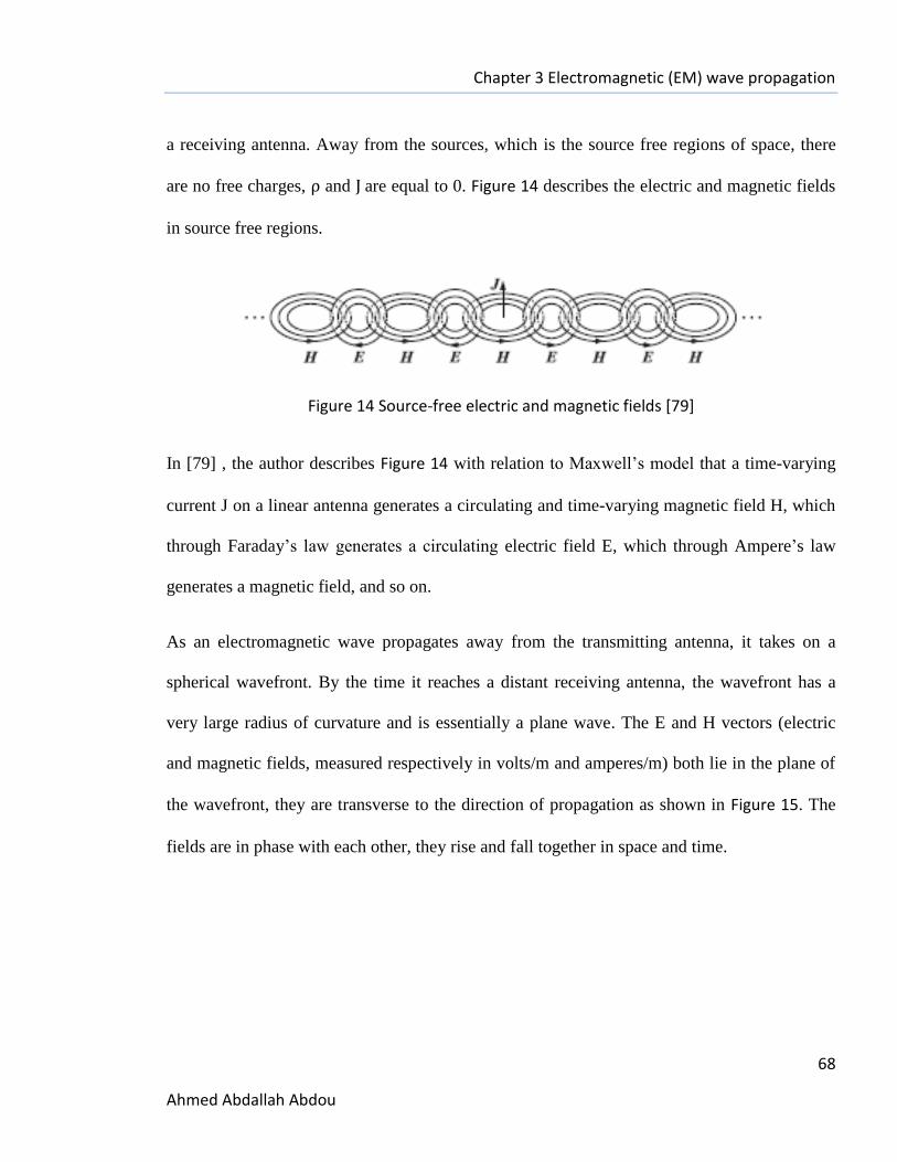
Chapter 3 Electromagnetic (EM) wave propagation
68
Ahmed Abdallah Abdou
a receiving antenna. Away from the sources, which is the source free regions of space, there
are no free charges, and are equal to 0. Figure 14 describes the electric and magnetic fields
in source free regions.
Figure 14 Source-free electric and magnetic fields [79]
In [79] , the author describes Figure 14 with relation to Maxwell’s model that a time-varying
current J on a linear antenna generates a circulating and time-varying magnetic field H, which
through Faraday’s law generates a circulating electric field E, which through Ampere’s law
generates a magnetic field, and so on.
As an electromagnetic wave propagates away from the transmitting antenna, it takes on a
spherical wavefront. By the time it reaches a distant receiving antenna, the wavefront has a
very large radius of curvature and is essentially a plane wave. The E and H vectors (electric
and magnetic fields, measured respectively in volts/m and amperes/m) both lie in the plane of
the wavefront, they are transverse to the direction of propagation as shown in Figure 15. The
fields are in phase with each other, they rise and fall together in space and time.

Chapter 3 Electromagnetic (EM) wave propagation
69
Ahmed Abdallah Abdou
Figure 15 Transverse electromagnetic (TEM) wave
Maxwell’s prediction lead to the velocity of these waves to be
√ where the constants
and in free space are respectively Farad/metre and
Henry/metre. This resulted in the experimentally-known speed of light c = 3×10⁸ m/sec
which revealed the electromagnetic nature of light.
Hertz conducted a series of experiments in the 1880s in which he generated and detected
electromagnetic waves with wavelengths very long compared to light. Then Guglielmo
Marconi was able to send a radio wave across the Atlantic Ocean in the 1900s. Since then, the
importance of Maxwell’s equations have been verified in optics, microwaves, antennas,
communications, radar and many sensing applications.

Chapter 3 Electromagnetic (EM) wave propagation
70
Ahmed Abdallah Abdou
3.4. Electromagnetic spectrum
The electromagnetic spectrum is considered as the entire range of electromagnetic radiation
ranging from the longest electric and radio waves through visible light to x-rays and the
shortest gamma and cosmic waves (Figure 16). These waves have different frequencies and
wavelengths but all travel at the same speed. Part of the spectrum includes the frequencies
used for radio communications. The boundaries of the radio spectrum are usually considered
to range from 9 kHz (9000 cycles per second) to 3000 GHz (3000 thousand million cycles per
second). Another part of the spectrum is the visible light with boundaries being the red and
violet with respective wavelength of 700nm and 350nm.
Figure 16 Electromagnetic spectrum [80]

Chapter 3 Electromagnetic (EM) wave propagation
71
Ahmed Abdallah Abdou
Although the whole spectrum is infinite, the useful spectrum is limited and some frequency
bands, such as the UHF, are already very congested. Normally, significant licence fees have to
be paid to use the spectrum, although there are some licence-free bands. The most well-known
ones are the Industrial, Science and Medical (ISM) bands allocated by the International
Telecommunication Union (ITU) as in Table 1. These bands are allocated in regions displayed
in Figure 17. The 433 MHz and 2.45 GHz are just two examples.
Table 1 Radio and microwave frequency bands allocated for Industrial Scientific and Medical
(ISM) applications by the International Telecommunication Union (ITU) [81]
Frequency band Central
frequency Wavelength World regions
covered
6.765 – 6.795 MHz 6.78 MHz 44.2 m Under consideration
13.553 – 13.567 MHz 13.56 MHz 22.1 m R1, R2, R3
26.957 – 27.283 MHz 27.120 MHz 11.1 m R1, R2, R3
40.66 – 40.70 MHz 40.68 MHz 7.4 m R1, R2, R3
433.05 – 434.79 MHz 433.92 MHz 0.69 m R1
902 – 915 MHz 915 MHz 0.33 m R1, R2, R3
2400 – 2500 MHz 2450 MHz 0.12 m R1, R2, R3
5725 – 5875 MHz 5800 MHz 0.05 m R1, R2, R3
24 – 24.25 GHz 24.125 GHz 1.24 cm R1, R2, R3
61 – 61.5 GHz 61.25 GHz 0.49 cm Under consideration

Chapter 3 Electromagnetic (EM) wave propagation
72
Ahmed Abdallah Abdou
122 – 123 GHz 122.5 GHz 0.24 cm Under consideration
244 – 246 GHz 245 GHz 0.12 cm Under consideration
Figure 17 Frequency band regions allocated by ITU [81]

Chapter 3 Electromagnetic (EM) wave propagation
73
Ahmed Abdallah Abdou
3.5. Electromagnetic wave propagation underwater
3.5.1. Permittivity of water
A lossy dielectric is defined in [82] as a medium in which an EM wave loses power as it
propagates. It has a conductivity σ≠0 in comparison to a lossless dielectric which has
conductivity σ=0.
The permittivity of a material is the characteristic which describes how it affects any electric
field set up in it. When the material is lossy, the relative permittivity is a complex quantity
[83] given by:
rrr ''j' (13)
The real part is related to the energy stored within the medium. Because water is a polar
molecule and rotates when exposed to an alternating electric field, the imaginary part is then
associated to the dissipation of the energy due to collisions during that rotation.
At 433MHz, the relative complex permittivity of water is 92.1j17.80 [84].
However as it is not explained which type of water it is referred to, a precise knowledge of the
relative complex permittivity of water also known as complex dielectric constant r is
therefore essential.
The primary work on complex dielectric constant was attributed to P. Debye in 1929. He
initiated a model (Debye model) with a single relaxation wavelength to calculate the
permittivity of water [85] as follows:

Chapter 3 Electromagnetic (EM) wave propagation
74
Ahmed Abdallah Abdou
(14)
With
j = √-1
ω=2πf, the angular frequency with f in Hz
εs, the static (zero frequency) dielectric constant
ε∞, the dielectric constant at infinite frequencies
ε0, the vacuum electric permittivity in farads/metre
τ, the relaxation time in seconds
α, the empirical parameter that describes the distribution of relaxation times
σ, the ionic conductivity in siemens/metre
However in further work [86] and [87], the authors confirmed that the Debye model was
unreliable because certain parameters including the static permittivity, the relaxation time and
the conductivity are dependant on the temperature and salinity of the water and must be
included in the model.
In [88], the authors came up with an improved model which fits the dielectric constant with a
single Debye relaxation law for frequencies up to 10GHz. It takes into account parameters
01
S j)j(1

Chapter 3 Electromagnetic (EM) wave propagation
75
Ahmed Abdallah Abdou
v).2(
)S,T(i)S,T(
)S,T(v
vi1
)S,T()S,T(
)S,T(v
vi1
)S,T()S,T(S,T
0
2
1
1
1S
including static permittivity, relaxation time, and conductivity which are dependent on the
temperature and salinity of the water.
Further work in [89] and [90] have shown that the Klein-Swift model was getting inaccurate
as frequencies increases.
Meissner and Wentz [91] introduced a model with a double Debye relaxation wavelength that
they considered necessary to provide an accurate fit for the dielectric constant over a wider
frequency range than the single Debye model. This model takes into account the salinity and
temperature contrary to the Debye model.
(15)
With
i = √-1
v, the radiation frequency in GHz
εs(T,S), the static (zero frequency) dielectric constant
ε∞, the dielectric constant at infinite frequencies
ε1, the intermediate frequency dielectric constant
ε0, the vacuum electric permittivity in farads/metre

Chapter 3 Electromagnetic (EM) wave propagation
76
Ahmed Abdallah Abdou
v1(T,S) and v2(T,S), the first and second Debye relaxation frequencies
T, the temperature in ⁰C
S, the salinity in ppt (parts per thousand)
σ, the conductivity in siemens/metre
3.5.1.1. Salinity effects on permittivity
The complex permittivity is dependent on the frequency, salinity and temperature as
formulated in the Meissner and Wentz model in equation (15). To predict the behaviour of the
permittivity of different types of water with regards to the frequency, the temperature is
maintained at a fixed value. This temperature is 20⁰C and is one of the measurements of the
canal water taken during a visit in summer to the Stanley canal in Liverpool, UK. The second
measurement is the conductivity of the water recorded at 0.0606 S/m and converted as in
section 1.2 to a salinity of 0.335ppt for use in the model where S is in ppt.
Using the Meissner and Wentz model, the permittivity of water with different salinity
concentrations S in ppt is calculated at a temperature of 20⁰C. A concentration of salinity
S=0ppt is used to refer to distilled water as in [92]. A concentration of salinity S=0.0871ppt is
used to refer to potable water from converting 0.013S/m which is the measured conductivity
of the water running from the laboratory tap. To refer to freshwater, a concentration of salinity
S=0.335ppt is used from the conversion of the measured 0.0606 S/m of the Stanley canal
water. To refer to seawater, the measured value of 4S/m in [1] is converted to a concentration
of salinity S=20ppt and is also within the range of salinity concentration “20ppt ≤ S ≥ 40ppt”

Chapter 3 Electromagnetic (EM) wave propagation
77
Ahmed Abdallah Abdou
used to refer to seawater in [91]. Although the model is valid for a wide range of frequencies
including below 1MHz, we focus on the spectrum between 1MHz and 100GHz. Real ε and
imaginary ε permittivity are calculated using the Meissner and Wentz model for the referred
types of distilled, potable, fresh and seawater and represented respectively in Figure 18, Figure
19, Figure 20 and Figure 21.
Figure 18 Permittivity of water with S=0ppt referred to as distilled water at T=20⁰C
0
10
20
30
40
50
60
70
80
90
1.00E+06 1.00E+07 1.00E+08 1.00E+09 1.00E+10 1.00E+11 1.00E+12
ε
Frequency (Hz)
Real ε
Imag ε

Chapter 3 Electromagnetic (EM) wave propagation
78
Ahmed Abdallah Abdou
Figure 19 Permittivity of water with S=0.0871ppt referred to as potable water T=20⁰C
Figure 20 Permittivity of water with S=0.335 referred to as freshwater canal at T=20⁰C
0
10
20
30
40
50
60
70
80
90
1.00E+06 1.00E+07 1.00E+08 1.00E+09 1.00E+10 1.00E+11 1.00E+12
ε
Frequency (Hz)
Real ε
Imag ε
0
10
20
30
40
50
60
70
80
90
1.00E+06 1.00E+07 1.00E+08 1.00E+09 1.00E+10 1.00E+11 1.00E+12
ε
Frequency (Hz)
Real ε
Imag ε

Chapter 3 Electromagnetic (EM) wave propagation
79
Ahmed Abdallah Abdou
Figure 21 Permittivity of water with S=20ppt referred to as seawater at T=20⁰C
In all cases the dielectric polarisation orientation is happening at 20GHz. This corresponds to
the first Debye relaxation as stated in [91]. This is also the region in Figure 19 where water
will be best heated up and by consequence the 2.45GHz frequency of operation is not the only
option available for microwave oven design. However this frequency proved to be both
effective and relatively cheap to achieve.
The real parts of the complex dielectric permittivity are related to the energy stored within the
medium. This value is approximately 80 for all cases except in seawater where it approximates
to 75, remains static up to 2GHz, and then drops at relaxation time. The salinity concentration
does not have a big impact on the real part permittivity. This means that saline water has
slightly less energy storage capability than pure water.
0
10
20
30
40
50
60
70
80
90
1.00E+06 1.00E+07 1.00E+08 1.00E+09 1.00E+10 1.00E+11 1.00E+12
ε
Frequency (Hz)
Real ε
Imag ε

Chapter 3 Electromagnetic (EM) wave propagation
80
Ahmed Abdallah Abdou
The imaginary parts of the complex dielectric permittivity are related to the dissipation of
energy due to collision during the rotation of the water polar molecule when exposed to an
alternating electric field. For pure water at the low end frequency of our spectrum these values
are near zero due to the absence of salinity. Then from the GHz, they start rising up to a
maximum, with a corresponding fall of the real parts, to meet at the first Debye relaxation
frequency (20GHz). In the presence of salinity, these values are now very large at the low
frequency end of the spectrum, and then drop for the 400-500MHz region where it reaches a
minimum. This happens in potable water but also in canal freshwater. We predict that within
this region (400-500MHz) lies the best frequency to operate in the potable and freshwater
canal environment.
In seawater these values are even bigger at the low frequency end of the spectrum, and then
drop at the 2-4GHz region where it reaches a minimum which is approximately 10 times
bigger than the previous case.
3.5.1.2. Temperature effects on permittivity
Other than frequency and salinity, the complex permittivity is also dependent on temperature
as formulated in the Meissner and Wentz model. Here, a prediction of the behaviour of the
permittivity with regards to the frequency for each type of water body will be given when its
temperature changes. The permittivity of each type of water body is calculated at varying
temperature from 0⁰C to 30⁰C in increments of 15⁰C.

Chapter 3 Electromagnetic (EM) wave propagation
81
Ahmed Abdallah Abdou
Figure 22 Effect of temperature on the real and imaginary parts of the permittivity of water
with salinity concentration S=0ppt referred to as distilled water
In Figure 22, the increase of temperature produces a proportional decrease of the real part of
the permittivity for frequencies up to 1GHz. The relaxation frequency at T=0⁰C is happening
at 10GHz and this corresponds to the first Debye relaxation in the Meissner and Wentz model
but also the Debye relaxation frequency in the Debye model where temperature and salinity
are not taken into account (T=0⁰C and S=0ppt). For distilled water, the increase in temperature
produces a relevant increase of the relaxation frequency.
0
10
20
30
40
50
60
70
80
90
100
1.00E+06 1.00E+07 1.00E+08 1.00E+09 1.00E+10 1.00E+11 1.00E+12
ε
Frequency (Hz)
Real ε at T=0⁰C Imag ε at T=0⁰C
Real ε at T=15⁰C Imag ε at T=15⁰C
Real ε at T=30⁰C Imag ε at T=30⁰C

Chapter 3 Electromagnetic (EM) wave propagation
82
Ahmed Abdallah Abdou
Figure 23 Effect of temperature on the real and imaginary parts of the permittivity of water
with salinity concentration S=0.0871ppt referred to as potable water
In Figure 23, the increase of temperature produces a proportional decrease of the real parts
permittivity for frequencies up to 1GHz. For the imaginary part permittivity, which is very
high compared to that of the real parts because of the salinity effects, a proportional change is
visible for the region up 100MHz. This is followed by their minimums shifting in terms of
frequency. For referred to as potable water, the increase in temperature also produces a
relevant increase of the relaxation frequency. However a region of minimum losses is apparent
in the 100MHz to 1GHz region.
0
10
20
30
40
50
60
70
80
90
100
1.00E+06 1.00E+07 1.00E+08 1.00E+09 1.00E+10 1.00E+11 1.00E+12
ε
Frequency (Hz)
Real ε at T=0C Imag ε at T=0C
Real ε at T=15C Imag ε at T=15C
Real ε at T=30C Imag ε at T=30C

Chapter 3 Electromagnetic (EM) wave propagation
83
Ahmed Abdallah Abdou
Figure 24 Effect of temperature on the real and imaginary parts of the permittivity of water
with salinity concentration S=0.335ppt referred to as canal freshwater
In Figure 24, the increase of temperature produces a proportional decrease of the real parts
permittivity for frequencies up to 1GHz. For the imaginary parts permittivity which is very
high compared to that of the real parts because of the salinity effects, a proportional change is
visible for the region up 100MHz. This is followed by their minimums shifting in terms of
frequency. For referred to as canal freshwater, the increase in temperature produces also a
relevant increase of the relaxation frequency. This shifts the minimum losses region higher by
50MHz.
0
10
20
30
40
50
60
70
80
90
100
1.00E+06 1.00E+07 1.00E+08 1.00E+09 1.00E+10 1.00E+11 1.00E+12
ε
Frequency (Hz)
Real ε at T=0C Imag ε at T=0C
Real ε at T=15C Imag ε at T=15C
Real ε at T=30C Imag ε at T=30C

Chapter 3 Electromagnetic (EM) wave propagation
84
Ahmed Abdallah Abdou
Figure 25 Effect of temperature on the real and imaginary parts of the permittivity of water
with salinity concentration S=20ppt referred to as seawater
In Figure 25, the increase of temperature produces a proportional decrease of the real parts
permittivity for frequencies up to 1GHz. For the imaginary parts are very high compared to the
real parts because of the conductivity effects, a proportional change is visible for 1GHz region.
This is followed by minimums shifting in terms of frequency. These minimums are higher
values compared to previous water salinities. For seawater, the increase in temperature also
produces a relevant increase of the relaxation frequency. However in this saline water body
0
10
20
30
40
50
60
70
80
90
100
1.00E+06 1.00E+07 1.00E+08 1.00E+09 1.00E+10 1.00E+11 1.00E+12
ε
Frequency (Hz)
Real ε at T=0C Imag ε at T=0C
Real ε at T=15C Imag ε at T=15C
Real ε at T=30C Imag ε at T=30C

Chapter 3 Electromagnetic (EM) wave propagation
85
Ahmed Abdallah Abdou
the losses are higher than in previous cases and the region is not considered as a minimum
region of losses.
For operating frequencies at ISM band (6.7MHz, 433MHz and 2.4GHz) and a temperature of
water of T=20⁰C, Real and Imaginary parts of water permittivity at different concentrations of
salinity to refer to different water environments, are calculated using the Meissner and Wentz
model and presented in Table 2.
Note that at 433MHz for water with salinity of 0ppt (referred to as distilled) at a temperature
of 20⁰C, the real part of the complex permittivity is 80.17 and the imaginary part is 1.92. This
is the permittivity quoted in section 3.5.1 from [84] and validates the model used in equation
(15).
Table 2 Real and Imaginary parts of permittivity at ISM frequencies
Those values are used to calculate the effective conductivity (σeff) and the attenuation (α).
Real Imaginary Real Imaginary Real Imaginary Real Imaginary
6.7MHz 75.19 7763.98 80.130 159.801 80.196 41.94 80.219 0.03
433MHz 75.15 121.88 80.080 4.393 80.146 2.57 80.170 1.92
2.4GHz 73.88 31.16 78.637 10.885 78.701 10.57 78.723 10.46
ISM
Frequency
Permittivity of water
with S=20ppt
(≈seawater), T=20⁰C
Permittivity of water
with S=0.335ppt
(≈freshwater), T=20⁰C
Permittivity of water
with S=0.0871ppt (≈tap
water), T=20⁰C
Permittivity of water
with S=0ppt (≈distilled
water), T=20⁰C

Chapter 3 Electromagnetic (EM) wave propagation
86
Ahmed Abdallah Abdou
3.5.2. Attenuation of EM wave propagation in water
The complex propagation constant describing the behaviour of an EM wave in [78] is
defined in equation (16) with a real attenuation constant α in equation (17) and an imaginary
phase constant β in equation (18) as follows:
(16)
(17)
(18)
The attenuation constant determines the rate of decay of a propagating electromagnetic wave
and the phase constant determines the rate of phase change. However we focus on attenuation
to predict EM wave propagation underwater because it refers to the decrease in the magnitude
of a signal as it propagates through a medium. In the case of conducting mediums including
water, equation (17) which is the homogeneous Helmholtz equation is modified to include the
effective conductivity which is the losses due to the imaginary portion being a measure of the
energy lost due to collision during rotation of the polar molecule (water). The modification
also includes the energy stored within the medium and is formulated as:
1εωσ10.5εμωα2
eff
(19)
1ωεσ10.5μεω2
1ωεσ10.5μεωα2

Chapter 3 Electromagnetic (EM) wave propagation
87
Ahmed Abdallah Abdou
With α, the attenuation in nepers/m
ω, the frequency in radians
μ, the permeability of the medium in N/A2
ε , the permittivity of the medium in F/m as r0 'ε
σeff , the effective conductivity in S/m as r0eff ''
Using the values of real and imaginary parts permittivity from Table 2 in equation (19),
attenuation (α) is then calculated for water with different concentrations of salinity (S)
including water with salinity S=0ppt to refer to as distilled water, water with salinity
S=0.0871ppt to refer to as potable water, water with salinity S=0.335ppt to refer to as
freshwater and water with salinity S=20ppt to refer to as seawater for the ISM (Industrial,
Scientific and Medical) band. These are presented in Table 3.
Table 3 Attenuations of ISM operating frequencies in water with different salinity
concentration
A representation of the attenuation (dB/m) in water with different concentrations of salinity
referring to different water environments in relation to the frequency (Hz) of operation is
displayed in Figure 26.
ISM
Frequency
Attenuation (dB/m) of
water with S=20ppt
(≈seawater), T=20⁰C
Attenuation (dB/m) of
water with S=0.335ppt
(≈freshwater), T=20⁰C
Attenuation (dB/m) of
water with S=0.0871ppt
(≈tapwater), T=20⁰C
Attenuation (dB/m) of
water with S=0ppt
(≈distilled water), T=20⁰C
6.7MHz 75.608 8.563 2.768 0.002
433MHz 459.632 19.335 11.316 8.465
2.4GHz 775.274 267.439 259.588 256.797

Chapter 3 Electromagnetic (EM) wave propagation
88
Ahmed Abdallah Abdou
Figure 26 Attenuation (dB/m) in water with different concentrations of salinity S, in relation
to the operating frequency (Hz)
According to Table 3 and Figure 26, attenuation in water with 20ppt of salinity (referred to as
seawater) is found to be very large but propagation seems to be feasible in the lowest
frequency band (6.7MHz). This theoretical feasible prediction has been practically proved
with experiments published in [60]. Propagation of EM waves in seawater [1] was more
affected by attenuation in the near field and experiments have shown that insulating the
antenna reduced the attenuation.
Attenuation in water with salinity concentration equal to or smaller than 0.335ppt including
water referred to as freshwater canal, potable and distilled water is not high in the middle ISM
ISM 6.70E+06
ISM 4.33E+08
ISM 2.40E+09
0
50
100
150
200
250
300
350
400
450
500
1.00E+06 1.00E+07 1.00E+08 1.00E+09 1.00E+10
Attenuation dB/m
Frequency (Hz)
water with S=0ppt (~distilled water)water with S=0.0871ppt (~potable water)water with S=0.335ppt (~freshwater canal)water with S=20ppt (~sea water)

Chapter 3 Electromagnetic (EM) wave propagation
89
Ahmed Abdallah Abdou
band at 433MHz. This seems encouraging for building a wireless sensor network using
commodity nodes operating at this frequency.
3.6. Experimental verification
3.6.1. Underwater experiments using an off-the-shelf kit at 2.4GHz ISM
Initial investigations concentrated on the most prevalent frequency for commercial WSN
transceivers which is 2.4GHz. To validate equation (19) used for predicting the attenuation of
radio signals in water, an experiment was set up in a tank of potable water. An off- the-shelf
wireless kit operating at 2.4GHz ISM band was used to evaluate the performance.
3.6.1.1. A temperature application in air and in water at a fixed 100mm
distance
3.6.1.1.1. Experimental setup
The tank had a length of 690mm, a width of 530mm and a height of 530mm. It was filled with
100 litres of potable water with 0.013S/m of conductivity. The conductivity of the water was
measured using a HI33000 conductivity meter. The Ez430-RF2500 wireless kit in Figure 27
contains a USB interface to program the nodes as Access Point or End Point. Once
programmed, one board had to be connected to the USB wireless board while the other was
fitted to the battery powered board and became a completely isolated wireless set. The boards
were based on the MSP430F2274 microcontroller and the CC2500 wireless transceiver
operating at 2.4GHz. They were all fitted with temperature sensors. Data such as hub number,
temperature, received signal strength indicator (RSSI) and voltage could be exchanged

Chapter 3 Electromagnetic (EM) wave propagation
90
Ahmed Abdallah Abdou
between the two nodes. The kit has a Sensor Monitor application which allows the
temperature of the two nodes and their separation distance to be monitored on the computer.
Figure 27 eZ430RF2500 Wireless sensor kit
The kit is designed for transceivers to communicate in air wirelessly using a Surface Mount
Device multilayer chip antenna for 2.4GHz with an average gain of 1dBi. More information
on the antenna can be found in [93]. At first, the sensor boards were put in air tight waterproof
plastic containers of sizes 140×95×45mm and separated by 100mm, in open air on a table as in
Figure 28. Then to determine whether EM wave propagation underwater is practically possible
at 2.4GHz, the air-tight enclosures containing the sensors were hung 100mm apart in 375mm
water depth in the plastic tank as in Figure 29. The End point is completely isolated and wire
free.

Chapter 3 Electromagnetic (EM) wave propagation
91
Ahmed Abdallah Abdou
Figure 28 Experimental setup of sensors in containers on table in air
These experimental setups and the results obtained are published in [94].
3.6.1.1.2. Results
Figure 30 displays the hub number, temperature, battery voltage and RSSI of the eZ430-
RF2500 communication hyper terminal when the Access Point (HUB0) and the End Point
(0001) sensors are both in air. The temperature sensor monitor application screen shot for
these sensors is shown in Figure 31.
Figure 29 Experimental setup of sensors in containers in a small tank with potable water
Plastic container Air
Table (wood) Sensors
100mm USB cable
Sensor
Plastic container
Potable water
100mm USB cable
Sensor
Weight
Plastic tank
690mm
530mm

Chapter 3 Electromagnetic (EM) wave propagation
92
Ahmed Abdallah Abdou
Hub number Temp
(ºC)
Battery
voltage
(V)
RSSI
(%)
0001 23.4 3.0 32
HUB0 28.0 3.6 -
0001 23.4 3.0 32
HUB0 28.0 3.6 -
HUB0 32.5 3.5 -
HUB0 26.3 3.6 -
HUB0 28.4 3.6 -
HUB0 26.7 3.6 -
0001 23.4 3.0 30
HUB0 28.4 3.6 -
HUB0 28.0 3.6 -
Figure 30 Data for sensors in air
Figure 31 Temperature sensor monitor in air
Figure 32 displays the hub number, temperature, battery voltage and RSSI of the eZ430-
RF2500 communication hyper terminal when the Access Point (HUB0) and the End Point
(0001) sensors are both in water. The temperature sensor monitor application screen shot for
these sensors is shown in Figure 33.

Chapter 3 Electromagnetic (EM) wave propagation
93
Ahmed Abdallah Abdou
Hub number Temp
(ºC)
Battery
voltage
(V)
RSSI
(%)
0001 22.6 3.0 17
HUB0 22.6 3.6 -
HUB0 25.9 3.6 -
0001 22.6 3.0 17
HUB0 25.9 3.6 -
0001 22.6 3.0 17
HUB0 24.7 3.5 -
0001 22.6 3.0 17
HUB0 28.8 3.5 -
0001 22.6 3.0 17
HUB0 25.9 3.6 -
Figure 32 Data for sensors in water
Figure 33 Temperature sensor monitor in water
The RSSI which is recorded and displayed on the Ez430-HyperTerminal has no units. In the
application report [95], the authors define that signal strength as the measured received signal
strength indicator RSSI given by the CC2500 radio. They state that it is output as a percentage
for readability and that the Access Point has always an output of 000%. In the source code

Chapter 3 Electromagnetic (EM) wave propagation
94
Ahmed Abdallah Abdou
[96] and the cc2500 datasheet [97], the relation between RSSI (%) and RSSI (dBm) is
formulated as:
( ) ( ( ) )
(20)
Using equation (20), the signal strength recorded from the end point nodes is converted into a
power level RSSI (dBm) for air and for potable water at 100mm separation distance and
displayed in Figure 34 for comparison with the datasheet values.
Figure 34 RSSI (dBm) of eZ430RF2500 Wireless sensor kit in air and in potable water at
100mm separation distance compared to datasheet values
3.6.1.1.3. Discussion
In the datasheet [97] the maximum RSSI(dBm) of the eZ430RF2500 at 2.4GHz is +1dBm and
the minimum RSSI is -104dBm. The maximum and minimum achievable RSSI in open air are
given as -99.8dBm and -15.36dBm. In our experiment, when the sensors were put within the
closed containers, 100 mm apart in air on a table, the strength value at the end point “0001”

Chapter 3 Electromagnetic (EM) wave propagation
95
Ahmed Abdallah Abdou
from the access point called “HUB0” is at an average strength value of “31” which is
equivalent to -48.64dBm. The temperature of the access point is recorded as 23.4⁰C. Then
when the sensors were put in the air-tight waterproof closed containers and suspended in water
depth of 375mm and 100mm apart, the strength value is at 17 which is equivalent to
-84.48dBm. This means that there has been a signal drop of 35.84dB due to the change of
medium. The temperature at the receiver in water has also dropped to 22.6⁰C because of the
temperature of the water. The theoretical value obtained at 2.4GHz for the potable water
attenuation in Table 3 was 259.59dB/m. This means that for the 100mm distance in potable
water the signal is expected to attenuate by 26dB. The experimental result has exceeded
theoretical prediction by 10dB; this difference can be explained by factors that may include
the small number of readings in the underwater experiment. However at such a high frequency
of 2.4GHz, the signal drop of 35.84dB due to the change of medium (from air to water) has
not affected data communication and was still reliable under water for a fixed range of
100mm.
3.6.1.2. Maximum separation of transceivers in air and in water at
2.4GHz
3.6.1.2.1. Experiment setup
In these experiments, all the equipment in the previous experiment are used but only the small
plastic tank of sizes L=690mm, W=530mm and H=530mm is replaced in order to measure the
maximum communication range of the transceivers operating at 2.4GHz.The bigger plastic

Chapter 3 Electromagnetic (EM) wave propagation
96
Ahmed Abdallah Abdou
tank is of sizes L=1620mm, W=620mm and H=580mm and filled with potable water of
0.013S/m conductivity as in Figure 35.
Figure 35 Experimental setup of sensors in containers in a big tank with potable water
In this set of experiments, sensors in air are moved apart with an increment of 100mm up to
1m and the RSSI, also called signal amplitude (dBm), was recorded. Then the sensors within
the plastic containers are submerged in the tank of potable water (Figure 35) and the signal
strength is recorded every 100mm to find the maximum communication range. The last
experiment is repeated but with a lower increment of 20mm in order to take more readings to
include the drop of signal amplitude happening within the first 100mm of separation distance
of the transceivers.
3.6.1.2.2. Results
Figure 36 graphically represents the signal amplitudes (dBm) of the sensors when moved apart
in increments of 100mm up to 1000m in both air and water.
Plastic container
Potable water
USB cable
Sensor
Weight
Plastic tank
1620mm
580mm

Chapter 3 Electromagnetic (EM) wave propagation
97
Ahmed Abdallah Abdou
Figure 36 Signal amplitude of eZ430RF2500 (2.4GHz) sensors in air and in water
Figure 37 represents graphically signal amplitudes (dBm) of the sensors when moved apart in
20mm increments up to its maximum communication range in water (200mm).
Figure 37 Signal amplitude of eZ430RF2500 (2.4GHz) sensors in water at 20mm increments
-110
-100
-90
-80
-70
-60
-50
-40
-30
100 200 300 400 500 600 700 800 900 1000
Am
plit
ud
e(d
Bm
)
Distance(mm)
In air In water
-110
-100
-90
-80
-70
-60
-50
20 40 60 80 100 120 140 160 180 200 220 240
Am
plit
ud
e
Distance(mm)

Chapter 3 Electromagnetic (EM) wave propagation
98
Ahmed Abdallah Abdou
3.6.1.2.3. Discussion
Figure 36 shows how the signal of the Ez430RF2500 at 2.4GHz travelling in air and in water
attenuates with distance. At 100mm separation distance, the signal in air had an amplitude of
-43.5dBm, whereas in water, it was significantly lower at -84.5dBm. In air the signal lost
26dB in 1000mm whereas in water it lost 28dB in 100mm as in Figure 37 (from 20mm to
120mm) and could not be detected after 200mm. This experimental value now exceeds the
theoretical value of 26dB by 2dB only.
In air, a Near Field Far Field (NFFF) transition region can be seen around 500mm in Figure
36. In water there is no NFFF, and attenuation is almost linear as in Figure 37. These
experiments have proven that underwater radio communication is possible at high ISM
frequency of 2.4GHz up to a range of 200mm only.
Attenuation at the 433MHz ISM frequency band in potable water is calculated in Table 3 as
11.31dB/m, thus for 100mm communication the loss predicted is 1.13dB which will predict a
better margin to increase the communication range.
Furthermore the medium change from air to water produced a drop in the signal which could
be explained by the fact that the chip antenna used in the ez430rf2500 kit is poorly matched in
water.

Chapter 3 Electromagnetic (EM) wave propagation
99
Ahmed Abdallah Abdou
3.6.2. Impact of the antenna and the frequency on the underwater
communication
3.6.2.1. Experiment setup
The ez430RF2500 wireless sensor kit with its chip antennas used in the previous experiment
was replaced. Here a Rohde and Schwarz SMB100A signal generator set at ISM frequencies
of 6.7MHz,433MHz and 2.4GHz creates a carrier signal and transmits it in the water at a
power of 0dBm as in Figure 39, through a 320mm diameter double loop antenna used in [61]
and displayed with frames in Figure 38. The amplitude of this signal was measured using a
Hewlett Packard HP8594E spectrum analyser.
Two experiments were performed. The first is to assess the impact of changing the antenna
(chip antenna previously used replaced with the double loop antenna with the same output
power) in an underwater communication. At 2.4 GHz, signal amplitude was recorded at each
increment of 200mm up to 1000mm. Then a frequency sweep of the antenna was done to find
its optimum frequency. The second experiment looked at the impact of using lower ISM
frequency bands in the transmission stage of an underwater communication system. The
amplitude of the received signal for each ISM frequency (6.7MHz, 433MHz and 2.4GHz) is
recorded as the antennas were moved in 200mm steps up to 1000mm. Furthermore, losses in
three different sizes (1m, 2.4m and 11m) of RG58 cables were measured for the ISM
frequencies.

Chapter 3 Electromagnetic (EM) wave propagation
100
Ahmed Abdallah Abdou
Figure 38 Double loop antennas of 320mm diameter with their frames
Figure 39 Experimental setup at ISM frequencies with double loop antennas
3.6.2.2. Results
Signal amplitudes (dBm) recorded at increments of 200mm up to 1000mm when using chip
antennas and double loop antennas at 2.4 GHz are represented graphically for comparison in
Figure 40. Amplitudes (dBm) of the signal received for each ISM frequency (6.7MHz,

Chapter 3 Electromagnetic (EM) wave propagation
101
Ahmed Abdallah Abdou
433MHz and 2.4GHz) when moving antennas at 200mm steps up to 1000mm are represented
in Figure 41. Measured losses for cables (1m, 2.4m and 11m) at ISM frequencies are
represented in Figure 42.
Figure 40 Comparison of chip antennas and double loop antennas at 2.4 GHz underwater
Figure 41 Signal amplitude at ISM frequencies up to 1000mm with 320mm double loop
antenna
-110
-100
-90
-80
-70
-60
-50
-40
-30
-20
100 200 300 400 500 600 700 800 900 1000
Am
pit
ud
e(d
Bm
)
Distance (mm)
chip antennas
D.loop antennas
-80
-70
-60
-50
-40
-30
-20
200 300 400 500 600 700 800 900 1000
Am
plit
ud
e(d
Bm
)
Distance(mm)
2.4 GHz433 MHz6.7 MHz

Chapter 3 Electromagnetic (EM) wave propagation
102
Ahmed Abdallah Abdou
Figure 42 Losses in cables (1m, 2.4m and 11m) at ISM frequencies
3.6.2.3. Discussion
Figure 40 allows the comparison of two types of antennas operating at 2.4GHz in an
underwater environment. It can be seen that using the chip antenna with the Ez430RF2500, the
signal at 100mm was -84.5dBm and it lost 15.5dB in 100mm, whereas the double loop
antennas starts with -59dBm and loses 1dB only. It could be stated that approximately 25dB
has been gained in the signal launch by changing the type and size of the antenna. But
surprisingly the signal remains strong after 200mm contradicting the theoretically predicted
attenuation at 2.4GHz frequency of 25dB in 100mm and the experiment using the wireless
transceivers with the chip antennas.
Figure 41 compares the three ISM frequencies when using the double loop antenna. It can be
seen that lower ISM frequencies of 433MHz and 6.7MHz show better signal strength at signal
6.7 100 433 2400 0
5
10
15
20
25
30
35
Loss
es
(dB
m)
Frequency (MHz)
1 m cable
2.4m cable
11m cable

Chapter 3 Electromagnetic (EM) wave propagation
103
Ahmed Abdallah Abdou
launch. However the 6.7MHz curve drops more quickly than the 433MHz. Although the
experiments demonstrate that lower ISM frequencies are less prone to signal attenuation in
water only at signal launching, the attenuations over distances present some errors. In the
experimental setup in Figure 39 the double loop antennas have their RF cable floating in air
which may have resulted in crosstalk. Therefore the results obtained with the double loop
antenna in water are not purely from the attenuated signal in water at least for the 2.4GHz
frequency.
According to Figure 42, losses in RG58 cables used in the experiments increase with their
length. Losses in long cables become considerably high at 433MHz and 2.4GHz. Therefore for
experiments at such high frequencies, the length of cables must be kept as small as possible.
3.7. Summary
The theoretical model predicted high attenuation in water at the highest ISM band of 2.4GHz.
This has been validated in the experiment with the communication being completely lost at
200mm of separation. However this 2.4 GHz ISM band has proved successful for a limited
distance. The distance was limited because of factors including the receiver sensitivity at -
100dBm whereas some receivers’ sensitivity can go down to -122dBm [98] . Most importantly
as confirmed in the theory and in the experiments, the 2.4GHz is a highly attenuated frequency
band in water. Although it provides many advantages including high data rate and availability
in complete kits, it can be used in applications requiring a high data rate for proximity
communications i.e. Automated Underwater Vehicles collecting data from an underwater node
where acoustic and optical are not viable options. The theoretical calculations predicted that

Chapter 3 Electromagnetic (EM) wave propagation
104
Ahmed Abdallah Abdou
within the region (400-500MHz) lies the best frequency to operate in the potable and
freshwater canal environment. Out of the operating frequencies in the ISM bands, the 433MHz
band is less attenuated that the 2.4GHz and gives a better data rate than the 6.7MHz.
Experiments have shown that antennas have a huge impact on the transmission and reception
stage of the underwater communication system, therefore a study on underwater antennas will
be carried out.

Chapter 4 Traditional antennas and water
105
Ahmed Abdallah Abdou
Chapter 4. Traditional antennas and water
4.1. Introduction
As antennas are another crucial element in underwater radio and microwave communication, a
set of traditional antennas will be investigated in this chapter. The theory required to construct
antennas to operate in air or in water will be outlined first. Traditional antennas were made for
the 433MHz ISM band and tested in water. The antenna with the best signal amplitudes was
then selected to undergo a modelling stage in High Frequency Structure Simulator to analyse
the behaviour of the antenna in two different environments (air and water). Important
parameters including the return loss, 3D far field radiation pattern and gain, directivity of the
antenna from HFSS reports will be presented to assess the suitability of using traditional
antennas in underwater communication systems.
4.2. Antenna theory
In free space, wave velocity (m/s) is related with frequency (Hz) and wavelength λ (m) in
[99] by:
(21)
Dipoles are one of the simplest but most widely used types of antennas. In [99], a linear
conductor which, at a given instant has a positive charge at one end and an equal but negative
charge at the other end may act as a dipole antenna. As the typical structure of a dipole

Chapter 4 Traditional antennas and water
106
Ahmed Abdallah Abdou
consists of two metal wires which are normally of equal length l, the dipole length can be
determined for a given frequency using equation (21). The half wavelength dipole is the most
popular dipole because of the impedance about 73ohms which is well matched with a standard
transmission line with impedance 75 ohms or 50 ohms [2].
Another type of popular antenna is the monopole which consists of one metal wire erected on
a perfect conducting ground. A monopole is half of the dipole antenna with a perfect
conducting ground plane acting as a mirror to generate its image [2]. For a given frequency,
the size of a monopole could be determined using equation (21). However, the quarter
wavelength is a resonant antenna with an impedance of 37ohms, which matches well the 50
ohms transmission line.
For a loop antenna of diameter d (m), the wavelength equation is given in [99] by:
(22)
To decrease the size of loop antennas, multiple loops can be used. Formed with two turns, the
double loop antenna used in [61] has its equation written as:
(23)
In free space, the speed of light is about [2], in water the speed is reduced by a
factor of √ where is the relative permeability which is 1 [61]. is the relative
permittivity calculated in Table 2, real parts permittivity values for potable water at 20⁰C are
used for the experiment. Table 4 presents the real parts permittivity, the reduction

Chapter 4 Traditional antennas and water
107
Ahmed Abdallah Abdou
factor √ , the velocity v (m/s) in water and the wavelengths λ (mm) in water and in air at
ISM frequencies.
Table 4 Real parts permittivity, reduction factor√ , velocity v (m/s) in water, wavelength
in water and in air (mm) for ISM frequencies (Hz)
FREQ (Hz) 6.70E+06 4.33E+08 2.40E+09
εr (Real) 80.196 80.146 78.701
√ 8.955 8.952 8.871
v (m/s) in water 3.350E+07 3.351E+07 3.382E+07
Wavelength in water (mm) 5000 77.4 14.1
Wavelength in air (mm) 44800 693 125
4.3. Construction and tests of traditional antennas in water
4.3.1. Experiment
In order to experiment with antenna behaviour in the water environment, several types and
sizes of antennas were built from insulated copper (16 SWG= 1.626mm width) and soldered
onto N type connectors. The diameter of the insulated copper was used because it fits neatly
into the solder bucket of a standard N type connector. The 433MHz ISM frequency was
selected as a compromise between attenuation and data rate, as described in the previous
chapter. The wavelength in water is calculated in (Table 4) as about 77mm. Using this value

Chapter 4 Traditional antennas and water
108
Ahmed Abdallah Abdou
and equations (21)(22)(23), sizes of conventional antennas could be determined for their
construction. One wavelength monopole (77mm) with ground plane, a half wavelength
monopole (38.5mm), one wavelength loop (77mm) and one wavelength dipole (77mm) as
shown in Figure 43 were built. A large 320mm diameter double loop antenna was available
from [61] for comparison. The experimental setup in Figure 44 involves a Rohde and Schwarz
SMB100A signal generator for creation of the carrier signal at a frequency of 433MHz and a
power of 0dBm for transmission in a plastic tank of potable water ( ) through
an antenna from the ones built. Then through a second antenna with the same specification the
signal was received and measured with a Hewlett Packard HP8594E spectrum analyser. An
RF transformer was connected to the antennas to achieve maximum power transfer. The
amplitude of the signal was recorded at each increment of 200mm up to 1000mm by moving
the receiver’s antenna. These were repeated for all the antennas constructed.
Figure 43 Antennas built for experiments (from right to left: one wavelength monopole with
ground, a half wavelength monopole, one wavelength loop and one wavelength dipole

Chapter 4 Traditional antennas and water
109
Ahmed Abdallah Abdou
Figure 44 Experimental setup of built antennas
4.3.2. Results
The signal amplitude (dBm) for the different type and size of antennas built for 433MHz ISM
frequency, measured every 200mm for a distance of 1 metre in the tank of water are
graphically represented in Figure 45.
Figure 45 Signal amplitude for different type and size of antennas at ISM 433MHz frequency
for varying distances up to 1m
-65
-60
-55
-50
-45
-40
-35
-30
-25
-20
200 300 400 500 600 700 800 900 1000
Am
plit
ud
e(d
Bm
)
Distance(mm)
320mm dloop 24mm loop
77mm monopole 38.5mm monopole
77mm dipole

Chapter 4 Traditional antennas and water
110
Ahmed Abdallah Abdou
4.3.3. Discussion
In Figure 45, the 23.5mm loop antenna has shown the best signal start at 200mm with
amplitude of -27.5dBm compared to other antennas. The second best start is given by the
77mm monopole at -33.6dBm. Then 38.5mm monopole starts with -34dBm followed by the
77mm dipole and 320mm double loop antenna with respectively signal starting at -37dBm and
-46dBm. At every 200 mm of separation distance up to 1 metre, the 23.5mm loop antenna had
the best signal amplitude. The 77mm monopole had the second best signal amplitude at every
200mm separation distance up to a metre except for at 400mm. Then there is inconsistency
over separation distances on which antenna perform better.
4.4. Modelling a traditional loop antenna
From the previous underwater experiments in the tank discussed in section 4.3.3, the loop
antenna showed the best signal strength in water over every 200mm separation distance up to
a metre. Therefore for further investigations of the antenna, including its behaviour with
regard to the change of medium from air to water, the modelling stage of a loop antenna at
433MHz ISM was carried out using High Frequency Structure Simulator.
HFSS is an interactive software package from ANSYS for calculating and simulating in 3D
the electromagnetic behaviour of a structure. HFSS is a finite element solver that uses the
Finite Element Method. It can be used for antenna structures where it divides the structure into
a fine mesh. It then finds the solution to Maxwell equations at each point on the mesh and
keeps refining the mesh until the solutions converge. The software has the ability to do post-

Chapter 4 Traditional antennas and water
111
Ahmed Abdallah Abdou
processing commands including return loss, input impedance and radiation patterns for
analysing the electromagnetic behaviour in detail.
The return loss is defined as a measure of how much power is reflected back (logarithmic
scale) from the terminal [2]. Return loss of the loop antennas in water was investigated to find
at what frequencies maximum power transfer occurs. Antenna impedance is defined as the
ratio of the appropriate components of the electric to magnetic fields at a point [100]. The
Smith chart is a graphical demonstrator and can be used to represent the impedance of the
antenna and visualize how well matched the impedance of the antenna is in the surrounding
environment. The radiation pattern of the antenna is a plot of the radiated power as a function
of the angle at a fixed distance, which should be large enough to be considered far field [2].
The radiation pattern can be represented as a 3D plot and can help in determining the
directivity of the antenna.
4.4.1. Loop antenna modelling in water
To model the antenna in HFSS the important stages to follow includes the design of the
antenna, boundaries and excitations setup, analysis via solution setup and frequency sweep,
and results.
At first, a 3D model is designed to represent the antenna. For this a circle of radius 0.6mm is
created on the ZX plane and positioned at [12.3mm, 0, 0]. The position of the circle at 12.3mm
on the X axis will be the radius of the loop antenna and is found from solving equation (22) for
the 77mm wavelength in Table 4. The material of the circle is assigned as Perfect Electric

Chapter 4 Traditional antennas and water
112
Ahmed Abdallah Abdou
Conductor. The circle is edited and a sweep around Z axis is generated with an angle of -358⁰
to generate the loop design in Figure 46.
Figure 46 Ansoft HFSS window, panels and 3Dmodel of designed 12.3mm radius loop
antenna
Either lumped port or wave port may be used as excitations for antenna simulations. In [101],
antennas with differential feeds should be excited with lumped port. A rectangular sheet is
created on the XY plane and its surface is approximated as perfect electric boundary which is
then assigned as a lumped port with 50ohms resistance for the excitation of the loop antenna.
To imitate the water environment, an absorbing radiation boundary is created so that the
Menu bar
Project Manager with project tree
Property Window
Message Manager
Progress Window
3D modeller Window
Toolbars

Chapter 4 Traditional antennas and water
113
Ahmed Abdallah Abdou
system absorbs the wave at the boundary. By preventing reflection, this effectively makes the
boundary infinitely far away from the structure. The material of the far field boundary is
assigned as water with conductivity of 0.02S/m. The boundary had to be placed at least a
quarter wavelength away from the strongly radiating structure of the antenna for the
simulation to be reliable [101].
Once the geometry of the loop antenna and its surroundings were designed as in Figure 47 and
validated, the analysis parameters had to be defined which involve the solution setup and
frequency sweep. For this a solution setup is added where the solution frequency is set at
433MHz. Then a frequency sweep is added and set between 1MHz and GHz and the
simulation is run for analysis.
Figure 47 Side-view of the designed 12.3mm radius loop antenna within a radiation boundary

Chapter 4 Traditional antennas and water
114
Ahmed Abdallah Abdou
After successful completion of the simulation, reports can be generated. A modal solution data
report is created on a rectangular plot to display the magnitude of the Scattering parameter
S(1,1) represented as return loss (dB). Another modal solution report is generated on a Smith
chart to display the impedance of the antenna in a normalised complex form. A far field report
is also created on a 3D polar plot to illustrate the gain of the antenna as a function of angle.
This 3D plot is then applied to the model to show the radiation field of the antenna with
respect to its position.
4.4.2. Results and discussion for 12.3mm radius loop antenna modelled in
water
Figure 48 Return loss of the 12.3mm radius loop antenna simulated in water
0.00 0.20 0.40 0.60 0.80 1.00Freq [GHz]
-6.00
-5.00
-4.00
-3.00
-2.00
-1.00
0.00
dB
(S(1
,1))
Water 0.02 at 12.3 radiusReturn Loss ANSOFT
m1
m2
m3
m4
Curve Info
dB(S(1,1))Setup1 : Sw eep
Name X Y
m1 0.5532 -5.5230
m2 0.1667 -1.6460
m3 0.4330 -2.2947
m4 0.0481 -0.1080

Chapter 4 Traditional antennas and water
115
Ahmed Abdallah Abdou
Figure 49 Smith chart of the impedance of the 12.3mm radius loop antenna simulated in
water
Figure 50 3D radiation plot of the gain of the
12.3mm radius loop antenna simulated in water
Figure 51 3D radiation field of the 12.3mm radius loop
antenna simulated in water with respect to its position
5.002.001.000.500.200.00
5.00
-5.00
2.00
-2.00
1.00
-1.00
0.50
-0.50
0.20
-0.20
0.000
10
20
30
40
50
60
708090100
110
120
130
140
150
160
170
180
-170
-160
-150
-140
-130
-120
-110-100 -90 -80
-70
-60
-50
-40
-30
-20
-10
Water 0.02 at 12.3 radiusSmith Chart ANSOFT
m1m2
m3
m4
Curve Info
S(1,1)Setup1 : Sw eep
Name Freq Ang Mag RX
m1 0.5332 -156.1195 0.5394 0.3113 - 0.1918i
m2 0.1667 -12.4022 0.8274 4.6109 - 5.1945i
m3 0.4330 -156.8225 0.7684 0.1364 - 0.2014i
m4 0.0481 148.9189 0.9887 0.0061 + 0.2781i
1GHz
1MHz
Open circuit Short circuit
Inductive
Capacitive

Chapter 4 Traditional antennas and water
116
Ahmed Abdallah Abdou
Figure 48 shows that the 12.3cm radius loop antenna modelled from theoretical calculation of
the wavelength and taking into account the reduction factor in water, resonates a 533MHz
with a return loss of 5.5dB which approximates 70% of transmitted power. At the frequency of
operation 433MHz, the return loss reads 2.3dB approximating 40% of the power being
transmitted. In both cases, a bandwidth cannot be calculated as the return loss does not reach
the minimum of 10dB required which approximates 90% of power transmitted. The
impedance of the antenna at 533MHz and 433MHz could be calculated from the normalised
ones showing in Figure 49 multiplied by 50ohms to give respectively 15.5ohms and 6.5ohms.
These figures show that the loop antenna impedance is not matched to the 50ohms required
even though at these frequencies the return losses are the best obtained. Figure 50 illustrates
that the maximum gain at the far field is -3.46dB and is happening at the ZX plane whereas
minimum gain of -20dB occurs on the Y axis. The shape of the loop radiation field as in
Figure 51 looks like a doughnut on the ZX plane with some nulls on the Y axis.
4.4.3. Results and discussion for loop antenna radius 16mm modelled in
water
The loop antenna with radius 12.3mm resonated at 533MHz. Because the frequency of interest
is 433MHz, the modelling in section 4.4.1 is kept unchanged except for the radius which is
iterated until resonance occurs at 433MHz. The optimised radius is found at 16mm and the
return loss, smith chart and radiation patterns are presented.

Chapter 4 Traditional antennas and water
117
Ahmed Abdallah Abdou
Figure 52 Return loss of the 16mm radius loop antenna simulated in water
Figure 53 Smith chart of the impedance of the 16mm radius loop antenna simulated in water
0.00 0.20 0.40 0.60 0.80 1.00Freq [GHz]
-10.00
-8.00
-6.00
-4.00
-2.00
0.00
dB
(S(1
,1))
Water 0.02 at 16mm radiusReturn Loss ANSOFT
m1
m2
m3
Curve Info
dB(S(1,1))Setup1 : Sw eep
Name X Y
m1 0.4330 -9.0182
m2 0.7540 -3.9098
m3 0.1365 -2.1041
5.002.001.000.500.200.00
5.00
-5.00
2.00
-2.00
1.00
-1.00
0.50
-0.50
0.20
-0.20
0.000
10
20
30
40
50
6070
8090100110
120
130
140
150
160
170
180
-170
-160
-150
-140
-130
-120-110
-100 -90 -80-70
-60
-50
-40
-30
-20
-10
Water 0.02 at 16mm radiusSmith Chart ANSOFT
m1
m2
m3
Curve Info
S(1,1)Setup1 : Sw eep
Name Freq Ang Mag RX
m1 0.4330 -149.0725 0.3542 0.5046 - 0.2101i
m2 0.7540 -152.8127 0.6373 0.2338 - 0.2293i
m3 0.1365 -5.0592 0.7874 7.4037 - 2.7063i
1GHz
1MHz
Open circuit Short circuit
Inductive
Capacitive

Chapter 4 Traditional antennas and water
118
Ahmed Abdallah Abdou
Figure 54 3D radiation plot of the gain of the
16mm radius loop antenna simulated in water
Figure 55 3D radiation field of the 16mm radius
loop antenna simulated in water with respect to its
position
Figure 52 shows that the return loss does not reach the minimum of 10dB for the bandwidth
and its impedance in Figure 53 is 25ohms at 433MHz resonance. The antenna gain in Figure
54 is slightly higher -3.29dB compared to -3.46dB in Figure 50 as the antenna size is 3.5mm
bigger. The radiation of the antenna in Figure 55 is still like a doughnut on the ZX plane with
some nulls on the Y axis.
4.4.4. Results and discussion of the 12.3mm radius loop antenna modelled
in Air
The 12.3mm is modelled in air by changing the radiation boundary material for investigations
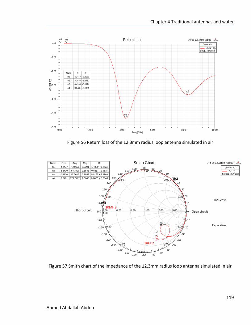
Chapter 4 Traditional antennas and water
119
Ahmed Abdallah Abdou
Figure 56 Return loss of the 12.3mm radius loop antenna simulated in air
Figure 57 Smith chart of the impedance of the 12.3mm radius loop antenna simulated in air
0.00 2.00 4.00 6.00 8.00 10.00Freq [GHz]
-6.00
-5.00
-4.00
-3.00
-2.00
-1.00
0.00
dB
(S(1
,1))
Air at 12.3mm radiusReturn Loss ANSOFT
m1
m2
m3m4
Curve Info
dB(S(1,1))Setup1 : Sw eep
Name X Y
m1 4.2477 -5.3655
m2 8.2430 -3.6980
m3 0.4330 -0.0374
m4 0.0481 -0.0031
5.002.001.000.500.200.00
5.00
-5.00
2.00
-2.00
1.00
-1.00
0.50
-0.50
0.20
-0.20
0.000
10
20
30
40
50
6070
8090100110
120
130
140
150
160
170
180
-170
-160
-150
-140
-130
-120-110
-100 -90 -80-70
-60
-50
-40
-30
-20
-10
Air at 12.3mm radiusSmith Chart ANSOFT
m1
m2
m3
m4
Curve Info
S(1,1)Setup1 : Sw eep
Name Freq Ang Mag RX
m1 4.2477 -42.0990 0.5391 1.4459 - 1.4733i
m2 8.2430 -64.3429 0.6533 0.6657 - 1.3678i
m3 0.4330 43.6606 0.9958 0.0153 + 2.4963i
m4 0.0481 173.7472 1.0000 0.0000 + 0.0546i
10MHz
10GHz
Open circuit Short circuit
Inductive
Capacitive

Chapter 4 Traditional antennas and water
120
Ahmed Abdallah Abdou
Figure 58 3D radiation plot of the gain of the
12.3mm radius loop antenna simulated in air
Figure 59 3D radiation field of the 12.3mm radius
loop antenna simulated in air with respect to its
position
Keeping the original radius of 12.3mm calculated for water and modelling the antenna in air
shows in Figure 56 that the antenna does not resonate any more on the 433MHz but at 4.2GHz.
This water to air frequency shift of approximately 9 times bigger is the inverse of the
reduction factor 1/9 applied in Table 4 for air to water and used to construct the antennas in
section 4.3. This validates the methodology used in constructing an antenna to operate in water
taking into account the reduction factor due to water. However the antenna exhibited a gain up
to -11.9dB in Figure 58 which means that the antenna designed for water is not appropriate in
an air environment. The radiation of the loop antenna in Figure 59 has changed to
omnidirectional on the XY plane with nulls along the Z axis. This phenomenon is due to the
reduced size of the wavelength from air to water and further explained in [2].

Chapter 4 Traditional antennas and water
121
Ahmed Abdallah Abdou
4.4.5. Results and discussion of loop antenna modelled from wavelength
calculation in air
The loop antenna is modelled in air. The radius is calculated from the wavelength in air in
Table 4 as 693mm and using equation (22) and yields a radius of 110mm. The simulation is
run in air and the resonance is at 457MHz. The loop radius is iterated to make it resonate at
433MHz and the return loss and impedance are then displayed.
Figure 60 Return loss of the 117mm radius loop antenna simulated in air
0.00 0.20 0.40 0.60 0.80 1.00Freq [GHz]
-6.00
-5.00
-4.00
-3.00
-2.00
-1.00
0.00
dB
(S(1
,1))
Air at 117mm radiusReturn Loss ANSOFT
m1
m2
Curve Info
dB(S(1,1))Setup1 : Sw eep
Name X Y
m1 0.4330 -5.4387
m2 0.8458 -5.0359

Chapter 4 Traditional antennas and water
122
Ahmed Abdallah Abdou
Figure 61 Smith chart of the impedance of the 117mm radius loop antenna simulated in air
Making a loop that resonates in air at 433MHz frequency from theoretical calculation, showed
in the result of the modelling, a shift of 24MHz in the resonance frequency. However iterating
the radius up to 117mm provided a resonance in the frequency of interest with a return loss of
5.38dB as shown in Figure 60. In neither resonance, does the return loss reach the required
10dB. Figure 61 shows that the impedance of the loop antenna modelled from theoretical
calculation of the wavelength in air approximates to 150ohms and refers to an impedance
mismatch in air. This confirms the statement in [2], that for mobile radio communications, the
loop is often used in pagers but hardly used in mobile transceivers which may be due to its
high resistance and reactance that makes it difficult to match to standard 50ohms transmission
lines over moderate bandwidth.
5.002.001.000.500.200.00
5.00
-5.00
2.00
-2.00
1.00
-1.00
0.50
-0.50
0.20
-0.20
0.000
10
20
30
40
50
60
708090100
110
120
130
140
150
160
170
180
-170
-160
-150
-140
-130
-120
-110-100 -90 -80
-70
-60
-50
-40
-30
-20
-10
Air at 117mm radiusSmith Chart ANSOFT
m1m2
Curve Info
S(1,1)Setup1 : Sw eep
Name Freq Ang Mag RX
m1 0.4330 -4.8144 0.5345 3.2398 - 0.4069i
m2 0.8458 -5.7090 0.5600 3.4468 - 0.5595i
10MHz
1GHz
Open circuit Short circuit
Inductive
Capacitive
Chapter 4 Traditional antennas and water
123
Ahmed Abdallah Abdou
Loop antennas were used in water in [61] [60] and were found to be strongly responding to
magnetic fields which makes them more advantageous for seawater. The antenna must be
matched in this particular water with its particular salinity and temperature properties.
However any change of these conditions will result in a mismatch of the antenna impedance.
This can significantly reduce the communication range. The radiation of the loop in water is
another factor making this type of antenna not suitable for our application.
4.5. Summary
Experiments in this chapter proved that underwater communication in the 433MHz ISM band
is possible at least up to a metre and validates the theoretical predictions in the previous
chapter. Although the loop antenna outperformed the other traditional antennas
experimentally, the modelling shows that even with an optimised size, the antenna impedance
in water and in air was mismatched. There was not any bandwidth available for the antenna in
any of the two modelling environments. Without means of matching, the communication
range required for the wireless sensor network would not be achieved. The radiation and
directivity of the loop antenna is not the same in air and in water and the omnidirectional
aspect of the antenna which cannot be maintained is another problem. The loop antenna and
other traditional narrowband antennas are unsuitable without matching means and therefore
bespoke antenna design with appropriate properties to suit underwater applications is sought.

Chapter 5 Bow-tie antenna
124
Ahmed Abdallah Abdou
Chapter 5. Bow-tie antenna
5.1. Introduction
In the previous chapter, simulations and experiments demonstrated the unsuitability of using
conventional and narrowband antennas for underwater communication without impedance
matching due to the high dielectric property of water compared to air. However antennas
utilising a matching circuit (RF transformers, balun, etc) may suffer from complete signal loss
if any changes in temperature and salinity occur in the water. As the antenna in question is to
be used in a wireless sensor network, another important aspect is the radiation of the antennas
which is to be taken into account to ensure movement of the sensors in the water without
complete signal loss. To select an antenna for wireless sensor network that could work in air
as well as in water, the focus will be on selecting an antenna that has a broad bandwidth, an
omnidirectional radiation pattern but also an antenna that can be prototyped for practical
validation tests. The antenna will be modelled in air and in water in HFSS. If proven
successful, the antenna will be prototyped for underwater tests in the laboratory tank.
5.2. Antenna selection and background
To find an antenna that could work in air and in water and to resolve impedance matching
hurdles in air designed antennas for underwater applications, we propose the bandwidth
technique. This means that the antenna has to have a broad bandwidth to accommodate the
change in such a heavy dielectric medium (water). Balanis suggested in [100] that a simple
configuration that can be used to achieve broadband characteristics is the biconical antenna

Chapter 5 Bow-tie antenna
125
Ahmed Abdallah Abdou
formed by placing two cones of infinite extent together. However as it is not possible to
manufacture an infinitely long biconical antenna, a geometrical approximation leads to the
bowtie antenna fabricated from metal sheet. This relates to the third antenna selection criterion
which is as crucial as the others. The ease of prototyping the antenna will help in validating it,
from selection to design and implementation for real life underwater tests. In [102], the bowtie
is defined as a planar version of the finite biconical antenna, which can be printed on a
dielectric substrate. Therefore the antenna could be fabricated on a PCB. The bowtie has other
advantages amongst other broadband antennas including biconical. The antenna could be
massively produced for the many nodes that will form the WSN. Also as the antenna has to be
used in water, the printed bowtie on PCB could be layered with waterproof material (glue or
plastic).
With regards to the second antenna selection criterion, the author states in [102], that the
radiation of the bowtie is a dipole-type radiation pattern, i.e. omnidirectional in the plane
perpendicular to that of the antenna.
In [99], an actual biconical with a full cone angle of 120⁰ has an omnidirectional pattern and
nearly constant 50ohms input impedance (power reflection less than 1 percent) over a 6 to 1
bandwidth with cone diameter D=λ at the lowest frequency. In [103], the bandwidth of the
bowtie antenna depends on the length of the plate. The flare angle and the length of the plate
define the lower frequency. A biconical and a bowtie antenna are depicted in Figure 62.
Bowtie antennas have been used in many Ultra Wideband (UWB) applications [104] including
ground penetrating radars [105] [106] and in mobile communication systems [107].

Chapter 5 Bow-tie antenna
126
Ahmed Abdallah Abdou
Figure 62 Diagrams of a Biconical and a Bow-tie antenna with flare angle α, cone diameter or
outer width D, plate length L
In 2012, Elrashidi et al presented a study in [75] on underwater wireless sensor network
communication using electromagnetic waves at resonance frequency 2.4GHz with a Bowtie
antenna. The work is purely based on simulations at a frequency of 2.4GHz which we have
already verified theoretically in section 3.5 and considered it as a highly attenuated band
underwater. We have also demonstrated experimentally in section 3.6 and in our 2011
publications in [63] that at 2.4GHz, common low power transceivers could communicate only
up to a very short range of 200mm. We have suggested that this band could be used for
proximity sensing underwater and not for UWSN. This has been confirmed by Lloret et al. in
their experimental work in 2012 [76] where they obtain 170mm communication range
between two transceivers operating at 2.4GHz. Furthermore Elrashidi at al. claim using a
bowtie in water whereas all their simulations are run in air. They have designed a bowtie
antenna in FEKO software to resonate at 2.4GHz ISM in air with a RL of -14dB. There is no
sign of simulation in water environment however the authors concluded with the results
obtained in air that the antenna gain of -30dB is a very high value for underwater wireless
α α α α D D
L L
- + - +

Chapter 5 Bow-tie antenna
127
Ahmed Abdallah Abdou
communication to overcome the high path loss due to attenuation. This (-30dB) value is a
negative gain exhibited at 90˚ theta in air and therefore their antenna should be considered as a
very lossy antenna which radiates poorly at 90˚ theta in air. Their maximum positive gain is
only 1.5dB at 0˚ and 180˚ theta in air.
The selection of the bowtie antenna to operate efficiently in an underwater wireless sensor
network is based on the three criteria set above which consist of an antenna with a broad
bandwidth to be able to work in air as well as in water in case of water level variations, an
omnidirectional radiation pattern to maintain signal strength as sensor nodes may be moved
with water current and an ease of prototyping the antenna for practical validation tests. Also
the bowtie antenna has to operate at lower than the 2.4GHz ISM band which is the 433MHz
band theoretically and experimentally demonstrated useful in chapter 3. As a consequence a
433MHz bowtie antenna will be modelled in air and in water in HFSS then prototyped for
underwater tests in the laboratory tank.
5.3. Modelling the Bow-tie antenna in air and in water
5.3.1. Design and simulations
The geometry of the bowtie antenna was created with the help of the HFSS Antenna Design
Kit (ADK). This is a GUI-based wizard tool that automates geometry creation, solution setup,
and post processing reports for 50 common antenna elements. The ADK then automatically
generates physical dimensions for desired frequency [108]. A bowtie antenna is chosen and
the desired frequency of operation at 433MHz is input. Then based on general design
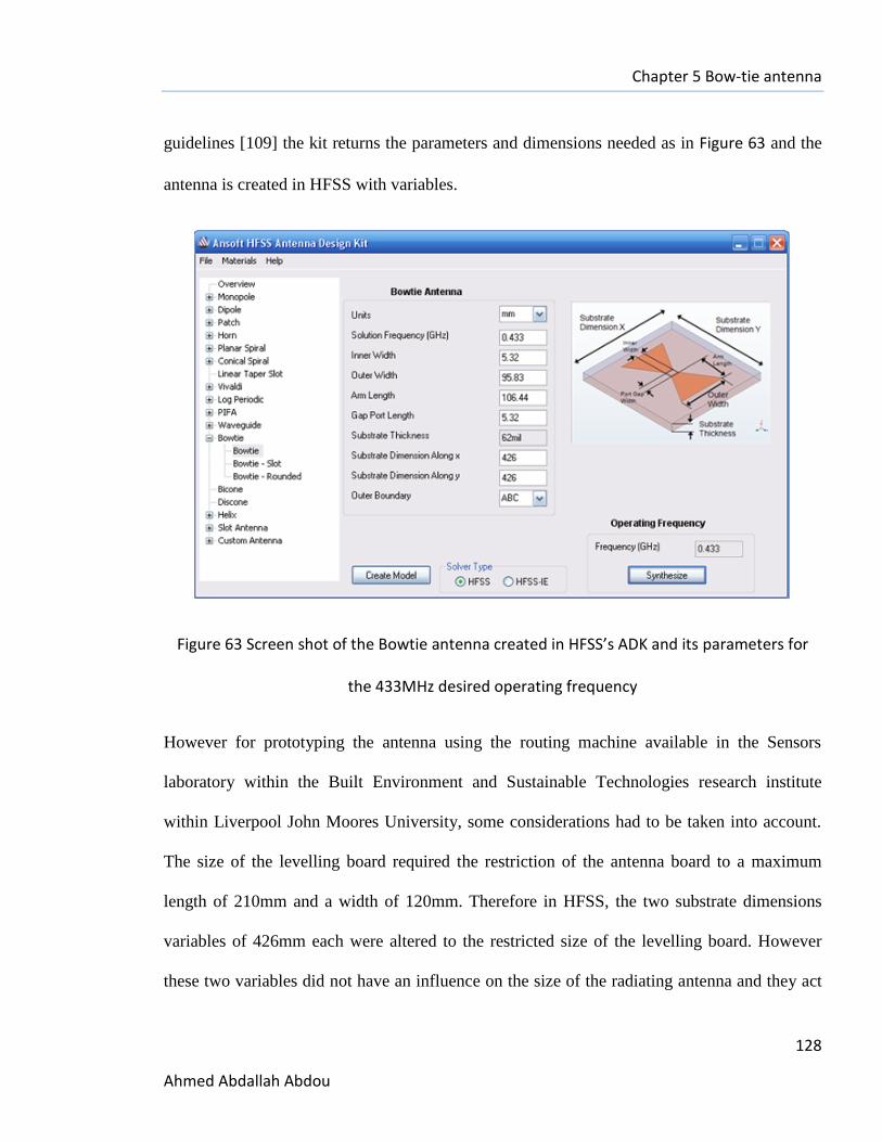
Chapter 5 Bow-tie antenna
128
Ahmed Abdallah Abdou
guidelines [109] the kit returns the parameters and dimensions needed as in Figure 63 and the
antenna is created in HFSS with variables.
Figure 63 Screen shot of the Bowtie antenna created in HFSS’s ADK and its parameters for
the 433MHz desired operating frequency
However for prototyping the antenna using the routing machine available in the Sensors
laboratory within the Built Environment and Sustainable Technologies research institute
within Liverpool John Moores University, some considerations had to be taken into account.
The size of the levelling board required the restriction of the antenna board to a maximum
length of 210mm and a width of 120mm. Therefore in HFSS, the two substrate dimensions
variables of 426mm each were altered to the restricted size of the levelling board. However
these two variables did not have an influence on the size of the radiating antenna and they act

Chapter 5 Bow-tie antenna
129
Ahmed Abdallah Abdou
as a support for the copper sheet. The arm length given by the ADK is bigger than the length
of the board and therefore in HFSS its size was changed from 106.44mm to 101.6mm. This
makes the outer width smaller at 91.5mm instead of the original 95.8mm. The inner width and
the port gap became 5.1mm. The new dimensions of the bowtie antenna were displayed in
Table 5.
Table 5 New dimensions of the bowtie antenna
Solution frequency 0.433 GHz
Inner width 5.1mm
Outer width 91.5mm
Arm length 101.6mm
Gap port length 5.1mm
Substrate thickness 1.57mm
Substrate Dimensions Along x 120mm
Substrate Dimensions Along y 210mm
Also the kit uses a substrate of 62mil thickness and creates the antenna on a 2.2 relative
permittivity. The standard single sided Printed Circuit Board that was used in the prototyping
stage is made of 0.0356mm thick copper sheet and FR4 glass-reinforced epoxy laminate sheet.
The PCB has a thickness of 1.6mm and a relative permittivity value of 4.4. Therefore in
HFSS, the substrate permittivity is changed to 4.4.

Chapter 5 Bow-tie antenna
130
Ahmed Abdallah Abdou
The antenna is modelled to resonate at 433MHz in an absorbing boundary condition with air
material properties to mimic free space environment. Then to predict the behaviour of the
bowtie antenna in water, the antenna is modelled in an absorbing boundary condition with
water of 0.02S/m conductivity. The angle-view of the bow-tie antenna and the radiation
bounds is shown in Figure 64.
Figure 64 Modelling of the 433MHz bow-tie antenna within a radiation box in HFSS
In HFSS, the bowtie antenna was modelled both in air and water to obtain the following
reports. Return losses of the antenna in air and in water were examined to observe where the
maximum power transfer of the antenna occurs. The input impedances of the antenna in air
and in water is presented in the Smith chart in order to visualize how well matched the
Bow-tie antenna on PCB for 433MHz
Air or water bound body

Chapter 5 Bow-tie antenna
131
Ahmed Abdallah Abdou
impedance of the antenna is in these two distinct environments. The direction of the antenna’s
radiation in air and water is shown in three dimension diagrams.
5.3.2. Results and discussion
The return losses of the antenna in air and in water are respectively represented in Figure 65
and Figure 66. The input impedances of the antenna in air and in water are respectively
represented in the Smith chart in Figure 67 and Figure 68. Three dimension diagrams of the
antenna radiation pattern simulation in air and in water are displayed respectively in Figure 69
and Figure 70.
Figure 65 Return loss of the simulated 433MHz Bow-tie antenna in air
0.00 0.20 0.40 0.60 0.80 1.00Freq [GHz]
-22.50
-20.00
-17.50
-15.00
-12.50
-10.00
-7.50
-5.00
-2.50
0.00
dB(S
(1,1
))
Bow_Tie_Antenna_in airReturn Loss ANSOFT
m1
m4
m2
m3
MY
1: -1
0.00
00
Curve Info
dB(S(1,1))Setup1 : Sw eep1
Name X Y
m1 0.4478 -20.7299
m2 0.4330 -15.7558
m3 0.4165 -10.1362
m4 0.4876 -10.1962
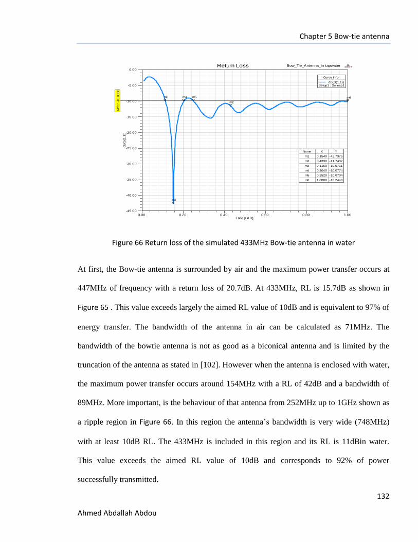
Chapter 5 Bow-tie antenna
132
Ahmed Abdallah Abdou
Figure 66 Return loss of the simulated 433MHz Bow-tie antenna in water
At first, the Bow-tie antenna is surrounded by air and the maximum power transfer occurs at
447MHz of frequency with a return loss of 20.7dB. At 433MHz, RL is 15.7dB as shown in
Figure 65 . This value exceeds largely the aimed RL value of 10dB and is equivalent to 97% of
energy transfer. The bandwidth of the antenna in air can be calculated as 71MHz. The
bandwidth of the bowtie antenna is not as good as a biconical antenna and is limited by the
truncation of the antenna as stated in [102]. However when the antenna is enclosed with water,
the maximum power transfer occurs around 154MHz with a RL of 42dB and a bandwidth of
89MHz. More important, is the behaviour of that antenna from 252MHz up to 1GHz shown as
a ripple region in Figure 66. In this region the antenna’s bandwidth is very wide (748MHz)
with at least 10dB RL. The 433MHz is included in this region and its RL is 11dBin water.
This value exceeds the aimed RL value of 10dB and corresponds to 92% of power
successfully transmitted.
0.00 0.20 0.40 0.60 0.80 1.00Freq [GHz]
-45.00
-40.00
-35.00
-30.00
-25.00
-20.00
-15.00
-10.00
-5.00
0.00
dB
(S(1
,1))
Bow_Tie_Antenna_in tapwaterReturn Loss ANSOFT
m1
m2
MY
1: -
10
.00
00
m6m3 m5m4
Curve Info
dB(S(1,1))Setup1 : Sw eep1
Name X Y
m1 0.1540 -42.7375
m2 0.4330 -11.7437
m3 0.1150 -10.0711
m4 0.2040 -10.0774
m5 0.2520 -10.0704
m6 1.0000 -10.2448

Chapter 5 Bow-tie antenna
133
Ahmed Abdallah Abdou
Figure 67 Smith Chart of the Input impedance for the simulated Bow-tie antenna in air
Figure 68 Smith Chart of the Input impedance for the simulated Bow-tie antenna in water
5.002.001.000.500.200.00
5.00
-5.00
2.00
-2.00
1.00
-1.00
0.50
-0.50
0.20
-0.20
0.000
10
20
30
40
50
60
708090100
110
120
130
140
150
160
170
180
-170
-160
-150
-140
-130
-120
-110-100 -90 -80
-70
-60
-50
-40
-30
-20
-10
Bow_Tie_Antenna_in airInput Impedance ANSOFT
Curve Info
S11Setup1 : Sw eep1
5.002.001.000.500.200.00
5.00
-5.00
2.00
-2.00
1.00
-1.00
0.50
-0.50
0.20
-0.20
0.000
10
20
30
40
50
60
708090100
110
120
130
140
150
160
170
180
-170
-160
-150
-140
-130
-120
-110-100 -90 -80
-70
-60
-50
-40
-30
-20
-10
Bow_Tie_Antenna_in tapwaterInput Impedance ANSOFT
Curve Info
S11Setup1 : Sw eep1
10MHz
1GHz
10MHz 1GHz
Open circuit Short circuit
Inductive
Capacitive
Open circuit Short circuit
Inductive
Capacitive

Chapter 5 Bow-tie antenna
134
Ahmed Abdallah Abdou
In Figure 67, it can be seen that the line representing the input impedance of the modelled
Bow-tie antenna in air starts for 10MHz frequency at where the resistive impedance is the
highest. The antenna is acting as an open circuit (at 0). The line is situated in the lower half of
the Smith chart and indicates that the antenna is capacitive. It then passes around the centre
(near 1) for frequencies 400 to 500MHz where the antenna is resistive and better matched to
radiate the most of its energy. The line finally finishes for frequencies above 500MHz towards
the open circuit. Whereas in Figure 68, the input impedance line of the Bow-tie antenna in
water starts at 10MHz, not as an open circuit, neither as a short circuit in the middle lower half
of the chart which shows the capacitive behaviour. The line then goes to the upper half of the
chart where it becomes inductive and then passes through the centre (at 1) around 150MHz for
purely resistive behaviour where the antenna radiates most of its energy. Then for frequencies
up to 1GHz the line rotates around a place not far from the centre to show that the antenna is
behaving better in the remaining frequencies range.
Figure 69 3D radiation pattern of the simulated Bow-tie antenna in air

Chapter 5 Bow-tie antenna
135
Ahmed Abdallah Abdou
Figure 70 3D radiation pattern of the simulated Bow-tie antenna in water
In Figure 69, the far field radiation of the antenna in air is represented in a 3D graph. The
radiation of the Bow-tie is a horn torus shape. The antenna radiates equally in all directions, it
can be called an omnidirectional antenna except for the arms where there are nulls. Whereas in
in water in Figure 70, the radiation pattern is smaller than for air, and has bigger nulls at the
arms of the antenna.
Overall the simulation results in air and water envisaged the bow-tie antenna to be a good
candidate for underwater wireless sensor networks.
5.4. Construction of the antenna
To construct the Bow-tie antenna on a printed circuit board, two main steps have been
followed. It consists of designing the antenna board on a specific software and then to etch the
copper with a routing machine.

Chapter 5 Bow-tie antenna
136
Ahmed Abdallah Abdou
5.4.1. EAGLE PCB design software
In the First step, a PCB design software EAGLE (Easily Applicable Graphical Layout Editor)
is used. The package made by CadSoft consists of a schematics editor, a PCB editor and an
auto-router module. This software is used to design an electronic schematic and lay out a
printed circuit board (PCB). It comes with an extensive library of components, a library editor
is also available to design new parts or modify existing ones. As there are no electrical
schematics to design, only the PCB Layout editor is used to draw the copper traces of the
antenna and the two holes for the connector as in Figure 71.
Figure 71 PCB layout of the Bow-tie antenna in EAGLE software

Chapter 5 Bow-tie antenna
137
Ahmed Abdallah Abdou
5.4.2. CNC routing machine
The second step consists of loading the board layout drawn in EAGLE to produce the antenna
board with the Computer Numerical Control routing machine Bungard CCD2 (Figure 72). To
load the layout into the machine, it was necessary to convert the board layout to the Hewlett-
Packard Graphical Language format by running the ‘mil-outlines.ulp’ in the Eagle software.
However Eagle software was not able to open the HPGL file and software ‘ABViewer7’ was
used as in Figure 73. Two files were produced to include the drilling and the routing. These
files were then loaded consecutively in CCD-control software RoutePro 2000 (Figure 74) to
produce the Bow-tie antenna on a single sided PCB as in Figure 75.
Figure 72 CNC Routing machine connected to a PC in the LJMU Sensors laboratory

Chapter 5 Bow-tie antenna
138
Ahmed Abdallah Abdou
Figure 73 HPGL format of the Bow-tie antenna in ABViewer7 software
Figure 74 CCD-control software RoutePro 2000

Chapter 5 Bow-tie antenna
139
Ahmed Abdallah Abdou
Figure 75 Angle view of the Bow-tie antenna fabricated with the CNC Routing machine
5.5. Waterproofing the PCB antenna for s11 tests
In order for the fabricated antenna to be tested underwater, the copper trace and the SMA
connector have to be isolated from water. Therefore the copper on the front side of the antenna
is fully covered with waterproof glue stick melted and poured carefully to form a 2mm
waterproof layer. The cap of a 50ml polypropylene centrifuge tube is also holed and glued to
the back side of the antenna so that its SMA connector can be joined to the RF cable. The
bottom of the centrifuge tube is removed and the tube is passed through a hole made in the
centre of an off-the shelf container lid. The RF cable is run through the container which an air
tight 1.4 litre food container made from polypropylene and measuring 120×140mm. A
watertight connector coupled with a 700mm long hose provided isolation of the RF cable from
water into the container. The cable had an N type end. The setup is displayed in Figure 76.

Chapter 5 Bow-tie antenna
140
Ahmed Abdallah Abdou
Figure 76 PCB Bow-tie antenna waterproofed with glue with its isolated RF cable
5.6. Experimental setup of bow-tie antenna’s S11 in air and in water
The bow-tie antenna designed, constructed and waterproofed in the previous sections was
tested in air and then tested in a plastic tank filled with 1200 litres of potable water with
conductivity of 0.035S/m and temperature of 15C. The fully waterproofed set is connected to
a MS2024A Anritsu Network Analyser to collect S11 antenna parameters in air and in water
as in Figure 77 for comparison. The position of the antenna is similar in both cases.

Chapter 5 Bow-tie antenna
141
Ahmed Abdallah Abdou
Figure 77 Experiment setup for S11 Return Loss in water
This experimental setup with the results obtained are published in [110].
5.7. Experiment results in air and in water for S11
The S11 data of the bow-tie antenna were collected during the experiments in air and in water
and plotted respectively in Figure 78 and Figure 79. The graph in Figure 80 regroups all the
S11 results for visual comparison.

Chapter 5 Bow-tie antenna
142
Ahmed Abdallah Abdou
Figure 78 S11 Experimental results in air of the constructed Bow-tie antenna
Figure 79 S11 Experimental results in water of the constructed Bow-tie antenna
-30
-25
-20
-15
-10
-5
0
10.00 226.00 442.00 658.00 874.00
S11
(d
B)
Frequency (MHz)
Experimented S11(dB) in air
-35
-30
-25
-20
-15
-10
-5
0
10.00 226.00 442.00 658.00 874.00
S11
(d
B)
Frequency (MHz)
Experimented S11(dB) in water
Bandwidth

Chapter 5 Bow-tie antenna
143
Ahmed Abdallah Abdou
Figure 80 Simulated and experimented S11 (dB) of a bow-tie antenna in air and in water
5.8. Discussion
From Figure 80 experimental results in air with comparison to simulation results in air show a
slight shift of 18MHz in the resonance frequency and a higher bandwidth of 20MHz as in
Figure 78. The slight difference which is acceptable can be associated to many factors
including the real life experiment and software simulations but also the layer of glue added on
the constructed PCB antenna to waterproof it. However in the experiment at 433MHz the RL
is 10dB and lies within the targeted RL for the antenna to be able to transmit more than 90%
of its power. Overall the experimented curve follows the simulated one in air.
-45
-40
-35
-30
-25
-20
-15
-10
-5
0
10 226 442 658 874
S11
(d
B)
Frequency (MHz)
Simulated S11 (dB) in air
Simulated S11 (dB) in water
Experimented S11 (dB) in air
Experimented S11 (dB) in water

Chapter 5 Bow-tie antenna
144
Ahmed Abdallah Abdou
In Figure 80 experimental results in water, in comparison with simulation results in water
show that there has been a slight shift of 14MHz in the resonance frequency with smaller
amplitude. The bandwidth of this valley was only 18MHz which is 82MHz smaller than the
simulated antenna in water. At 433MHz the RL is 15dB which allows the antenna to transfer
more than 96% of its power. More importantly, is the behaviour of the antenna from 226MHz
up to 1GHz shown as a ripple region in Figure 79. In this region the antenna becomes
broadband with at least 12dB of RL. The experimental results follow the overall shape of the
simulated curve and the ripple region shows the broadband aspect of the antenna. From Figure
80 the broadband aspect in water of the experimented curve is clearly situated under the
simulated one giving more assurance that this important aspect can be maintained in the
transition from simulation to the physical construction of the antenna. The Bow-tie antenna
has shown from simulations and experiments that it is suitable for underwater communication.
5.9. Further experimental investigation on the bow-tie antenna: the
temperature change effects in water
5.9.1. Experiment setup
To experiment with the effects of temperature on the bow-tie antenna behaviour, a trial was set
up as shown in Figure 81. It involved a network analyser taking S11 readings of the
waterproofed antenna placed in a bucket of potable water (σ= 0.017 S/m at 15⁰C). The
experiment was then repeated with water that was cooled to almost 0˚C, and then again by
water at 30˚C.

Chapter 5 Bow-tie antenna
145
Ahmed Abdallah Abdou
Figure 81 Experimental setup for temperature change effects on the antenna
5.9.2. Results and discussion
The S11 return loss data of the antenna at different temperatures in water are graphically
represented in Figure 82 for comparison. The data of the antenna in air are also plotted for
references in air.
Figure 82 S11 return loss data of the antenna at different temperatures in water
-30
-25
-20
-15
-10
-5
0
0.00E+00 2.00E+08 4.00E+08 6.00E+08 8.00E+08 1.00E+09
S11
(d
B)
Frequency (Hz)
S11[dB]_Air
S11[dB]_Water @T≈0⁰C
S11[dB]_Water@T≈15⁰C
S11[dB]_Water@T≈30⁰C

Chapter 5 Bow-tie antenna
146
Ahmed Abdallah Abdou
When the antenna is in air, because of the position of the antenna (facing the ground at 700mm
distance) the resonance frequency is at 450MHz with a RL of 23dB. At 433MHz, it is 14dB.
In water at approximately 360MHz, the RL is approximately 10dB all the way to 1GHz giving
a wideband bandwidth of 640MHz. This means that at any frequency within that region, a
transmission of approximately 90% is achieved. However the increase of temperature does not
result in a consistent change of the RL. In comparison with the air, there is no resonance
frequency and therefore a temperature change can increase the communication distance or
decrease it but only after reaching the distance achieved at 90% transmission.
Furthermore, the S11 reflected coefficient Г real and imaginary data of the antenna at different
temperatures in water are graphically represented in Figure 83 for the frequency range of
interest lying in the 400-500MHz region only. The data from the antenna in air before the
experiment and after the experiment are also plotted for reference. The 400-500MHz
frequency ranges in different water temperature is close to the centre (Г=0). Although after
graphical reading on the Smith chart, the next step is to match for 50ohm impedance (Г =0)
but this is more appropriate for narrow band antenna at a given frequency. Maintaining a wide
bandwidth to accommodate signal fluctuations in the water is a requirement as long as the
antenna return loss is more than 10dB (90% of transmission).
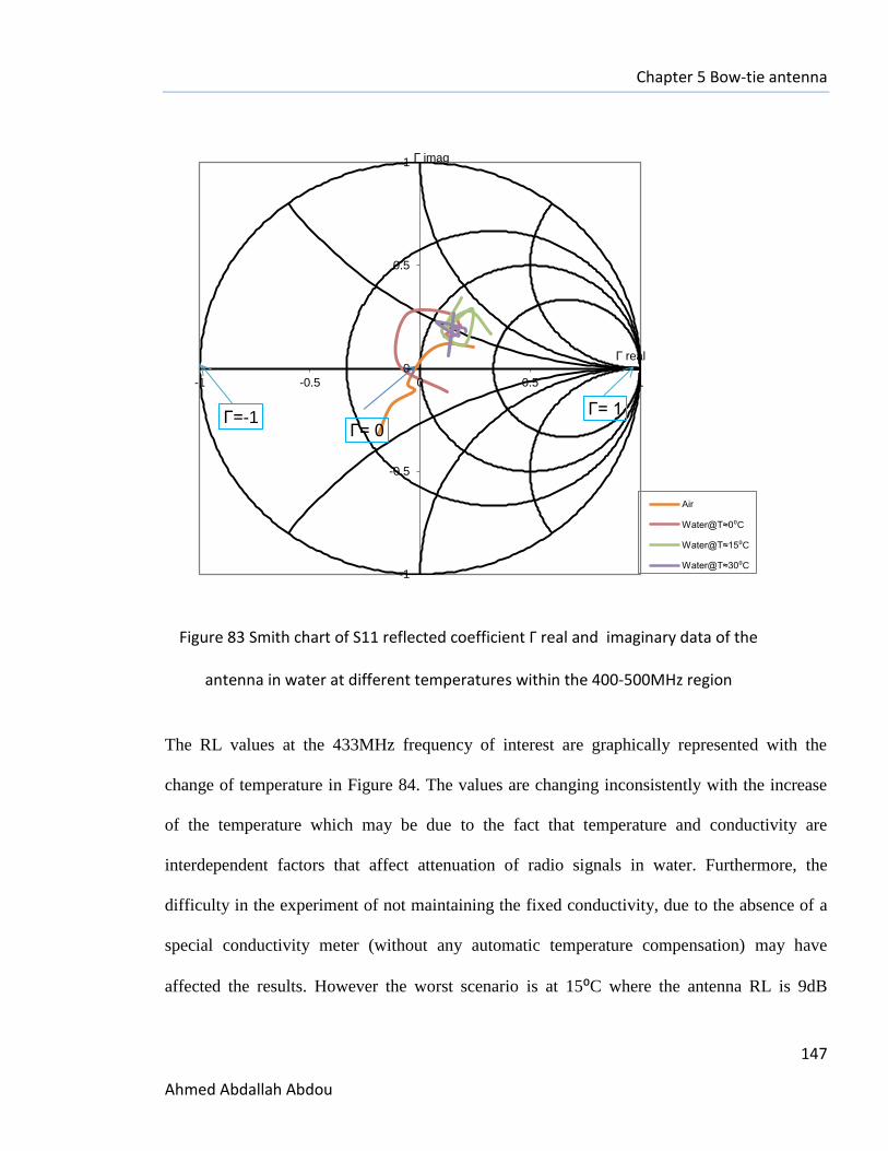
Chapter 5 Bow-tie antenna
147
Ahmed Abdallah Abdou
Figure 83 Smith chart of S11 reflected coefficient Г real and imaginary data of the
antenna in water at different temperatures within the 400-500MHz region
The RL values at the 433MHz frequency of interest are graphically represented with the
change of temperature in Figure 84. The values are changing inconsistently with the increase
of the temperature which may be due to the fact that temperature and conductivity are
interdependent factors that affect attenuation of radio signals in water. Furthermore, the
difficulty in the experiment of not maintaining the fixed conductivity, due to the absence of a
special conductivity meter (without any automatic temperature compensation) may have
affected the results. However the worst scenario is at 15⁰C where the antenna RL is 9dB
Γ=-1 Γ= 0
Γ= 1
-1
-0.5
0
0.5
1
-1 -0.5 0 0.5 1
Г imag
Г real
j0
ro
r0.5
r1
r2
0.5j
j
2j
-2j
-j
-0.5j
Γ=-1
Γ= 0
Γ= 1
Air
Water@T≈0⁰C
Water@T≈15⁰C
Water@T≈30⁰C

Chapter 5 Bow-tie antenna
148
Ahmed Abdallah Abdou
which corresponds to approximately 88% energy transmission. At other temperatures, there
are at least 92%.
Figure 84 S11 return loss at 433MHz of the antenna at different temperatures in water
Narrowband antennas and traditional loop utilising matching circuit for a specific frequency in
water can see their resonance frequency or amplitude shifting consistently with the increase of
temperature but the experiment of the broadband bow-tie antenna in potable water have
demonstrated immunity with the temperature change above the targeted RL of 10dB.
5.10. Summary
With narrowband and traditional loop antennas suffering from impedance matching which
results in signal losses in water, the bandwidth technique was proposed to accommodate the
change in such a heavy dielectric medium. The planar version of finite biconical broadband
antennas was investigated. The Bow-tie antenna was modelled to operate at 433MHz in air.
-30
-25
-20
-15
-10
-5
0
0 15 30
S11
RL
(dB
)
Temperature in ⁰C

Chapter 5 Bow-tie antenna
149
Ahmed Abdallah Abdou
Although the simulation results in air shown a limited bandwidth, in water it showed an ultra-
broadband behaviour. The antenna was successfully prototyped on PCB and waterproofed for
underwater tests. The S11 results of the experiments demonstrated that the Bow-tie antenna
that is designed and constructed for air could be used in water without any matching circuit.
Further experiments have shown its immunity towards temperature change in water.

Chapter 6 Wireless transmitter
150
Ahmed Abdallah Abdou
Chapter 6. Wireless transmitter
6.1. Introduction
Most of underwater RF experiments in the literature review [111] utilise on the transmitting
side a signal generator to create the signal to the antenna through a RG58 RF cable. Trials with
this type of setup have shown in chapter 4 that the RF cable acts as an antenna and
consequently may result in erroneous data received from crosstalk. In this chapter, a
transmitter that generates a carrier signal at 433MHz is built from an electronic circuit and is
powered by battery. It is then waterproofed for complete submersion in the laboratory tank for
underwater tests with no RF cable floating in air/water to eliminate airborne transmission.
6.2. Electronics
In order to generate a carrier signal, a voltage control oscillator (VCO) was used. This is an
electronic oscillator whose oscillation is controlled by an input voltage. A coaxial ZX95-535-
S+ VCO that covers the 433MHz ISM frequency was acquired from Minicircuits. To
experiment on the creation of the carrier in the laboratory a Tektronix PS280 DC Power
Supply was used to provide power to the VCO and a Hameg HMS 3000 Spectrum Analyser
was used to monitor the signal produced by the VCO. A fixed 12V input was supplied on the
Vcc port of the VCO and a variable voltage was applied on the VTune port to oscillate at
different frequencies. From the datasheet available in [112], a voltage of approximately 9V
gives a frequency of 426.3MHz. Tuning the voltage to 9.5V created a carrier signal at
433MHz with a power output of +6dBm as visible on the spectrum in Figure 85.

Chapter 6 Wireless transmitter
151
Ahmed Abdallah Abdou
Figure 85 Carrier signal creation using DC power supply
To design a wireless transmitter the fixed part of the power supply is substituted with batteries
and the variable part with a potentiometer. A Voltage Regulator is used to step down the
voltage from the batteries. The Block diagram in Figure 86 illustrates the design of the
transmitter’s carrier generator.

Chapter 6 Wireless transmitter
152
Ahmed Abdallah Abdou
Figure 86 Block diagram of the transmitter’s carrier generator
The VCO runs on 12V fixed therefore a Voltage Regulator is needed to adjust the excess of
voltage from the batteries. To supply enough power to the L7812 Voltage Regulator requiring
19V as in the datasheet available in [113], 16 AA 1.5V Energizer batteries are connected in
RF OUT
Antenna
Voltage Controlled Oscillator
ZX95-535-S+
-
Potentiometer
3296W-1-103LF
Voltage Regulator
L7812
Power
E91
Input
Output
Ground
+
V tune V In Ground
12
V
24
V
12
V

Chapter 6 Wireless transmitter
153
Ahmed Abdallah Abdou
series to deliver 24V. Two battery holders taking 8 batteries each were used to accommodate
the 16 batteries that have a service time of approximately 65 hours as explained in the
datasheet available in [114]. The 10kΩ potentiometer available in [115] is tuned to 9.5V to
output a 433MHz carrier signal ready to be transmitted via an antenna. A jumper is added to
the circuit for connecting the power on and off. The heat sink provides cooling to the voltage
regulator. The setup is attached to a piece of hard bound board. Wooden legs were made so the
batteries sit at the back. The setup weighing 525gram and measuring 100×100mm was
designed to fit in a plastic container measuring 120×140mm. Figure 87 shows the battery
powered transmitter’s carrier generator.
Figure 87 Battery powered transmitter’s carrier generator set

Chapter 6 Wireless transmitter
154
Ahmed Abdallah Abdou
The device was then connected to the spectrum analyser through an RG316 RF cable with
SMA connectors on both ends, to test the carrier signal. Figure 88 shows the battery powered
set generating the 433MHz carrier signal at +6dBm power output on the spectrum analyser.
Figure 88 433MHz carrier signal test on spectrum analyser
6.3. Waterproofing the wireless transmitter
An off-the shelf, air tight 1.4litre polypropylene food container measuring 120×140mm was
used to fit the 100×100mm electronics set. The lid of the plastic container was modified to run
the RF cable. The bottom of a 50ml polypropylene centrifuge tube was removed and the tube
is passed through a hole made in the centre of the container’s lid and then glued by melting
waterproof plastic glue stick. The cap of the centrifuge tube was also holed and glued to the
back side of the antenna so that its SMA connector could be joined to the RF cable as in
Figure 89. The front side of the antenna was fully covered with glue to make it waterproof.
The antenna cap was closed on the tube, and the lid was clipped with the container comprising
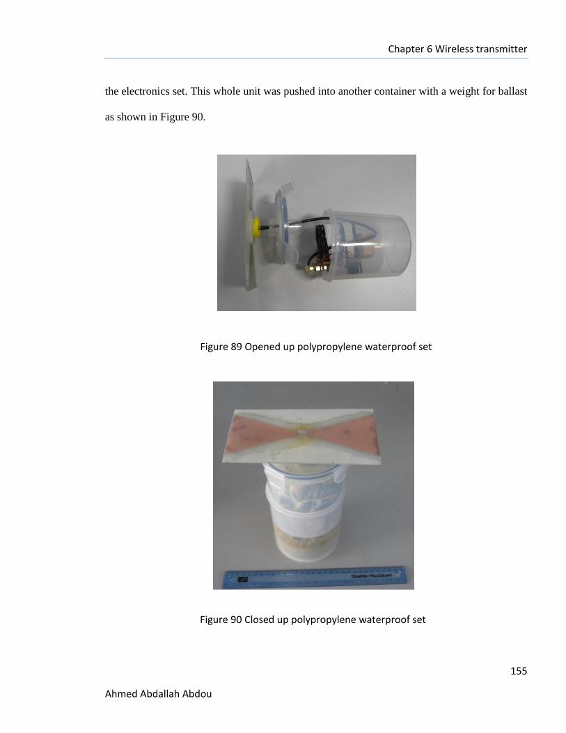
Chapter 6 Wireless transmitter
155
Ahmed Abdallah Abdou
the electronics set. This whole unit was pushed into another container with a weight for ballast
as shown in Figure 90.
Figure 89 Opened up polypropylene waterproof set
Figure 90 Closed up polypropylene waterproof set

Chapter 6 Wireless transmitter
156
Ahmed Abdallah Abdou
6.4. Experimental setup for S21 with off-the-shelve PP containers in laboratory
6.4.1. Transmission in air and in water at vertical separation
In order to experiment on the transmission of the carrier signal in air, a setup was prepared
taking into account that the following experiment will be in the tank with water. In air the
setup comprises the wireless transmitter positioned on a wooden chair at the same level as the
bottom of the tank. The carrier signal is generated and transmitted through the antenna. On the
receiver side a vertically moveable waterproofed bow-tie and plastic container were connected
to a Hewlett Packard 8594E Spectrum Analyser through an RG58 cable in the hose, supported
by a PVC tube. The receiver was positioned vertically above the transmitter with both sides’
antennas facing each other. Then the receiver was moved upward with the PVC tube at an
increment of 10mm to record the signal strength on the spectrum analyser (Figure 91). A
temperature of 13.8⁰C ±0.5 was recorded.
Figure 91 Experimental setup for S21 transmission in air

Chapter 6 Wireless transmitter
157
Ahmed Abdallah Abdou
The wireless transmitter containing the electronics was lowered into the tank. The PVC tube
which the receiver and its antenna are attached to, was pushed down to align with the wireless
transmitter’s antenna. Then the tube was pulled at an increment of 10mm to move the receiver
away the transmitter and record the signal strength on the spectrum analyser as shown in
Figure 92. In water, the temperature was 14.7˚C ±0.5 and the conductivity was 0.035 S/m.
Figure 92 Experimental setup for S21 transmission in water
6.4.2. Radiation pattern in air and in water at vertical separation
The setup for the radiation pattern in air is the same as the transmission in air (Figure 91) but
while in the previous setup the receiver is moved upward with the PVC tube, the receiver and
the transmitter are instead fixed at a 100mm separation distance within the near field. Only the
receiver tube is rotated to make the antenna turn at angles with increments of 10˚. The
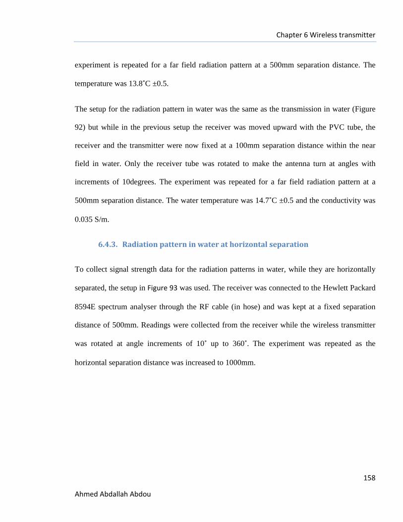
Chapter 6 Wireless transmitter
158
Ahmed Abdallah Abdou
experiment is repeated for a far field radiation pattern at a 500mm separation distance. The
temperature was 13.8˚C ±0.5.
The setup for the radiation pattern in water was the same as the transmission in water (Figure
92) but while in the previous setup the receiver was moved upward with the PVC tube, the
receiver and the transmitter were now fixed at a 100mm separation distance within the near
field in water. Only the receiver tube was rotated to make the antenna turn at angles with
increments of 10degrees. The experiment was repeated for a far field radiation pattern at a
500mm separation distance. The water temperature was 14.7˚C ±0.5 and the conductivity was
0.035 S/m.
6.4.3. Radiation pattern in water at horizontal separation
To collect signal strength data for the radiation patterns in water, while they are horizontally
separated, the setup in Figure 93 was used. The receiver was connected to the Hewlett Packard
8594E spectrum analyser through the RF cable (in hose) and was kept at a fixed separation
distance of 500mm. Readings were collected from the receiver while the wireless transmitter
was rotated at angle increments of 10˚ up to 360˚. The experiment was repeated as the
horizontal separation distance was increased to 1000mm.

Chapter 6 Wireless transmitter
159
Ahmed Abdallah Abdou
Figure 93 Experimental setup for radiation pattern at horizontal separation
6.5. Results for a S21 experiment with off-the-shelve PP containers in
laboratory
6.5.1. Transmission at vertical separation distances in air and in water
Figure 94 displays signal strength (S21) experiment for the bow-tie antennas in air and in
water in the tank over a distance of 450mm. The graph shows that in air the antenna signal
strength dropped by 10dB over a separation distance of 450mm. However it seems that this is
the maximum loss the antenna will suffer from in air. In water, at 10mm the signal loses 10dB
compared to the air environment. This value added to the power of the VCO (6dB at 433MHz)
is in agreement with the theoretical attenuation value of 16.6dB in Table 3. Two regions can
be distinguished, the near-field region up to 300mm separation distance, and a far-field region
onwards. The near field region includes the region where the signal drops more quickly. In the
far field, the signal is around -40dB, and the signal amplitude drops at a lower rate.

Chapter 6 Wireless transmitter
160
Ahmed Abdallah Abdou
Figure 94 Comparison of bowtie antenna’s signal strength (S21) experimented in air and in
water over distance up to 450mm
6.5.2. Radiation pattern in air and in water at vertical separation
Figure 95 illustrates the radiation pattern of the bowtie antennas on a 360˚ plane, separated by
100mm, both in air and water. It can be seen that the highest signal occurred when the two
antennas were 0˚ and 180˚ in line and the lowest signal, were at 90˚ and 270˚. In water at
100mm separation distance, the overall shape is the same as in air but with a smaller signal
and a small variation at the 90˚ angle.
-45
-40
-35
-30
-25
-20
-15
-10
-5
0
10 50 90 130 170 210 250 290 330 370 410 450
S21
(d
B)
Distance (mm)
Experimented S21(dB) in air
Experimented S21(dB) in water

Chapter 6 Wireless transmitter
161
Ahmed Abdallah Abdou
Figure 95 Comparison of bowtie antenna’s signal strength radiation pattern (S21) over
radiation angles in air and in water at a vertical separation of 100mm
In Figure 96 the bowtie antennas were separated by 500mm vertically. The highest signals in
air and in water still occurred at 0˚ and 180˚ with the lowest at 90˚ and 270˚. In water the
overall shape is the same with a smaller signal and an additional variation at 330˚.
-60
-50
-40
-30
-20
-10
00
10 2030
4050
60
70
80
90
100
110
120
130140
150160
170180190200210
220230
240
250
260
270
280
290
300
310
320330
340350360
Signal strength (dBm)in air,(100mm away)
Signal strength (dBm)in water,(100mm away)
Radiation angle in degree S21 in dBm

Chapter 6 Wireless transmitter
162
Ahmed Abdallah Abdou
Figure 96 Comparison of bowtie antenna’s signal strength radiation (S21) over radiation
angles in air and in water at a vertical separation of 500mm
At both separation distances, the signal strength of the bowtie antennas in water reduced
because of the attenuation due to water. The small variations could be associated with
reflections or errors. Also when the antennas were vertically separated, the radiation pattern in
air was the same as in water.
6.5.3. Radiation pattern in water at horizontal separation
In Figure 97 the bowtie antennas were separated by 500mm then 1000mm horizontally in
water over a radiation plane of 360˚. At a 500mm separation, the highest signals in water still
occurred at 0˚ and 180˚ with the lowest at 90˚ and 270˚. At 1000mm the overall shape was the
same with a smaller signal due to higher attenuation increased with distance and some
-70
-60
-50
-40
-30
-20
-10
00
10 2030
4050
60
70
80
90
100
110
120
130
140150
160170180190200
210220
230
240
250
260
270
280
290
300
310
320330
340350 360
Signal strength (dBm) inair,(500mm away)
Signal strength (dBm) inwater,(500mm away)
Radiation angle in degree S21 in dBm

Chapter 6 Wireless transmitter
163
Ahmed Abdallah Abdou
variations at 330˚ may be associated with reflections or errors. However, the bowtie antennas
performed better in the water tank at horizontal separation when they were at 0˚ and 180˚.
Figure 97 Comparison of bowtie antenna’s signal strength radiation (S21) over radiation
angles in water at horizontal separation of 500mm and 1000mm
6.5.4. Comparing bowtie radiation pattern in water at vertical and
horizontal separation
Figure 98 displays the radiation pattern on a 360˚ plane of the bowtie antennas in water at
vertical and horizontal separation of 500mm.The overall shapes are similar and in both cases
the antennas perform better at 0˚ and 180 ˚. The slight changes are related to the fact that the
dimensions of the tanks and the volume of water where vertical and horizontal tests have been
performed are not identical.
-60
-55
-50
-45
-40
-35
-300
10 2030
4050
60
70
80
90
100
110
120
130
140150
160170180190200
210220
230
240
250
260
270
280
290
300
310
320330
340350 360
Signal Strength(dBm)in tankwith water at500mmseparation
Signal Strength(dBm)in tankwith water at1000mmseparation
Radiation angle in degree S21 in dBm

Chapter 6 Wireless transmitter
164
Ahmed Abdallah Abdou
Figure 98 Comparison of bowtie antenna’s signal strength radiation (S21) over radiation
angles in water at horizontal and vertical separation of 500mm
From the radiation pattern experiments, the maximum performance can be achieved when the
bow-tie antennas at 0˚ and 180˚. This performance is achieved in cases where the antennas’
separation is vertical (antenna facing each other) as shown in Figure 92 but also horizontal
(antennas symmetric) as shown in Figure 93.
Whether in air or in the water tank the same overall shape of the radiation pattern is repeated
in contrast with the loop antennas that give a maximum signal when at water. Therefore the
positioning of the antennas can be done in air and changes in water should not be expected.
-70
-60
-50
-40
-300
10 2030
4050
60
70
80
90
100
110
120
130
140150
160170180190200
210220
230
240
250
260
270
280
290
300
310
320330
340350360
Signal Strength(dBm)in tankwater 500mmaway vertically
Signal Strength(dBm)in tankwater 500mmaway horizontally
Radiation angle in degrees S21 in dBm

Chapter 6 Wireless transmitter
165
Ahmed Abdallah Abdou
6.6. Summary
To eliminate RF crosstalk, a battery powered wireless transmitter that generated a carrier
signal at 433MHz was designed and prototyped. The set was waterproofed to run the S21
experiments. The carrier signal was transmitted and received wirelessly with success in tank
with water up to a half metre separation distance. The far field result suggested that a
detectable signal could be successfully received at much larger separation distances. The
radiation pattern experiments confirmed that the same positioning of the bow-tie antennas in
air can be maintained in water.

Chapter 7 Real world tests in Liverpool Stanley canal
166
Ahmed Abdallah Abdou
Chapter 7. Real world tests in Liverpool Stanley canal
7.1. Introduction
In the previous chapter, wireless communication in the 433MHz ISM band between a battery
powered transmitter and a receiver was successful in a tank full of potable water up to half
metre distance. Distances were limited by the tank size. This chapter describes how the
transceivers are now submerged in the Liverpool Stanley canal for maximum communication
range. Experiments to collect S11 and S21 data were carried out.
7.2. Design and prototyping of a waterproof PVC enclosure
7.2.1. Transmitter’s enclosure
For the transceivers to be submerged in open water, robust enclosures were designed. The
transmitter’s enclosure is shown in Figure 99. The container is mainly fabricated from
polyvinyl chloride (PVC) to minimize reflections and the chance of the container acting as a
cavity with comparison to stainless steel.

Chapter 7 Real world tests in Liverpool Stanley canal
167
Ahmed Abdallah Abdou
Figure 99 Exploded view of transmitter’s enclosure designed in SolidWorks
Circular PVC top
PMMA antenna cover
PCB Bowtie antenna
Rubber sheet
Rubber sheet
PVC cover (antenna seat
and cylinder cover )
PVC cylinder house of
transceiver electronics
O ring
O ring
PVC cylinder
bottom cover
Stainless steel support
Stainless steel top support
Top
Bottom
dle

Chapter 7 Real world tests in Liverpool Stanley canal
168
Ahmed Abdallah Abdou
7.2.1.1. The top part of the enclosure
The top part involves the waterproofing of the antenna and the top sealing of the enclosure.
The fact that the connectors are SMA type makes it susceptible to split especially considering
that the transmitter is expected to be tested in a non-static environment (water). For the
antenna to be in a fixed position, a thin layer of the plastic is removed in order to make it sit.
This cover as shown in Figure 100 was used to protect and support the antenna but also to seal
the cylinder of the enclosure. On the exploded view it is called PVC cover (antenna seat and
cylinder cover)
Figure 100 PVC cover
The polymethyl methacrylate (PMMA) part protects the top part of the antenna from water
and is sealed to the PVC cover with a gasket and jointing compound. Figure 101 shows the
PMMA antenna cover. The dielectric properties of this transparent material cause a small shift
in the resonant frequency in air, however in water this shift is not visible as it happens under
the target RL of 10dB because of the broadband behaviour of the bowtie antenna.

Chapter 7 Real world tests in Liverpool Stanley canal
169
Ahmed Abdallah Abdou
Figure 101 PMMA
A thin layer of rubber gasket covered in non-setting gasket jointing compound by Hylomar
provided a water tight seal. 8 Stainless steel bars 70mm long with a diameter of 5.4mm are
used with nuts to mechanically seal the layers forming the top part of the enclosure. In the
exploded view they are called Stainless steel top support.
The circular PVC top shown in the exploded view is used to completely close the top with the
stainless steel bars. The shape as shown in Figure 102 is made to provide tight sealing but also
to minimise signal disturbance of the antenna in the middle.
Figure 102 PVC Cover

Chapter 7 Real world tests in Liverpool Stanley canal
170
Ahmed Abdallah Abdou
7.2.1.2. The bottom part of the enclosure
The bottom part housed the electronics. This PVC cylinder contained the transceiver
electronics. (Figure 103)
Figure 103 Cylinder
Plastic O rings as shown in Figure 104 on each side of the cylinder were used to aim for
complete water tightness.
Figure 104 O Ring for cylinder

Chapter 7 Real world tests in Liverpool Stanley canal
171
Ahmed Abdallah Abdou
The PVC cylinder Bottom cover in Figure 105 was used to close the bottom of the container
with an O Ring.
Figure 105 PVC cylinder Bottom cover
Four stainless steel threaded bars give a mechanically strong seal when tightened with nuts but
also facilitate dismantling of the container after tests. In the exploded view they are named as
Stainless steel support.
The complete transmitter’s enclosure was assembled without the antenna (Figure 106) and
tested in the tank of the laboratory. At first, the container has shown small leakage. Then after
using the non-setting gasket jointing compound by Hylomar in a few trials, the leakage has
stopped. The container was subjected to a five hour submersion and did not suffer any leaks
either in the antenna seat or in the electronics house.

Chapter 7 Real world tests in Liverpool Stanley canal
172
Ahmed Abdallah Abdou
Figure 106 Transmitter’s enclosure
Figure 107 shows the underwater transmitter assembled with the antenna and the electronics
after being tested in the tank.
Figure 107 Underwater transmitter

Chapter 7 Real world tests in Liverpool Stanley canal
173
Ahmed Abdallah Abdou
7.2.2. Receiver’s enclosure
The receiver enclosure differs from the transmitter, it’s only the top part (as it does not include
any electronics) and its antenna is connected directly to a RG58 RF cable. A hose was cut to
length to cover the cable and a hose connector provides waterproofing. (Figure 108)
Figure 108 Receiver’s enclosure designed in SolidWorks
The complete receiver’s enclosure is assembled with the antenna (Figure 109) and tested in the
tank. The container, submerged for five hours, did not show any leaks in the antenna seat or
from the hose connector.
Figure 109 Underwater receiver

Chapter 7 Real world tests in Liverpool Stanley canal
174
Ahmed Abdallah Abdou
7.3. Effect of the fabricated PVC enclosure on the transmission
Upgrading from an off the shelf PP container to a more robust PVC enclosure to house the
electronics of the transceivers was successful in terms of waterproofing. However as
electromagnetic waves are susceptible to their surroundings, the change of enclosure may
affect the transmitted and received signals and therefore requires a close look. An experiment
in the laboratory water tank was carried out with the wireless transmitter in the PVC enclosure
tested for S21 transmission. The results are displayed in Figure 110. The new signal followed
the same pattern as the previous but with less loss which meant that greater distance will be
achieved.
Figure 110 Effects of the fabricated PVC enclosure on the transmission
-45
-40
-35
-30
-25
-20
-15
-10
-5
0
0 50 100 150 200 250 300 350 400 450
S21
Tra
nsm
issi
on
(d
Bm
)
Distances (mm)
S21 Transmission (dBm) of transceivers in waterwaterproofed by PP container
S21 Transmission (dBm) of transceivers in waterwaterproofed by PVC container

Chapter 7 Real world tests in Liverpool Stanley canal
175
Ahmed Abdallah Abdou
7.4. Experimental method for S11 and S21 with the fabricated PVC enclosures
in the canal
Previous experiments in water took place in laboratory tanks with limited distances. Also the
absence of water current in the tank is not giving a close match to a real-life water
environment. In Liverpool L5, United Kingdom, the Stanley canal (Figure 111) was identified
as a suitable site for long distance communication and immersion of transceivers. Permission
was sought from the Canal and River Trust North West body. After assessing the risks
involved and fulfilling all the Health and Safety requirements, the trials were approved.
Figure 111 Bing maps, top view of the Stanley canal locks and their surroundings [116]
(in circle: Top Lock Footbridge)

Chapter 7 Real world tests in Liverpool Stanley canal
176
Ahmed Abdallah Abdou
In the canal, the conductivity and temperature of the water were measured. Using the
conductivity meter HI33000, readings were taken at three different locations, and were found
to be 606±3µS/cm. A K type thermocouple attached to a TM-902C thermometer was used to
record the water temperature during the test, this was 16.3±0.4˚C. The electrical equipment
that was used for the experiment is listed below:
The Anritsu MS2711D Handheld Spectrum Analyser for 100 kHz to 3GHz (Figure 112)
connected to the receiver recorded the signal strength of the transmitted carrier signal
(433MHz).
Figure 112 Anritsu MS2711D Handheld Spectrum Analyser
The R&S ZVL Vector Network Analyser 9 kHz to 3GHz (Figure 113) was used to measure
the impedance of the antenna in this water environment.

Chapter 7 Real world tests in Liverpool Stanley canal
177
Ahmed Abdallah Abdou
Figure 113 R&S ZVL Vector Network Analyser 9kHz to 3GHz
To supply enough power for the above analysers, a Halfords portable powerpack 200 (Figure
114) was used generating 230-240V mains power with a 20Ah battery and inverters.
Figure 114 Halfords portable powerpack 200

Chapter 7 Real world tests in Liverpool Stanley canal
178
Ahmed Abdallah Abdou
Other equipment that was used for the experiments is pictured in Figure 115.
Figure 115 Other equipment used for the canal experiments
Conductivity meter
Shackle and pulley Temperature meter
50N Buoyancy aid × 3 Lifebuoy
Heavy duty
nylon rope
Tape measure

Chapter 7 Real world tests in Liverpool Stanley canal
179
Ahmed Abdallah Abdou
7.4.1. S11 Reflection coefficient for Smith Chart
The experiment was run in the Top Lock (Lock No 1) Footbridge to measure the changes of
the antenna’s behaviour in the canal. This test recorded the real and imaginary values of the
reflection coefficient Г. These were then displayed in the Smith chart for analysis.
Figure 116 S11 of receiver in Stanley Top Lock (Lock No 1) Footbridge
7.4.2. S11 Return loss
Reflection coefficient data experimented in Figure 116 was also converted to Return Loss
values in order to be graphically represented.

Chapter 7 Real world tests in Liverpool Stanley canal
180
Ahmed Abdallah Abdou
7.4.3. S21 Transmission at horizontal separation
The transmitter (Tx) and receiver (Rx) were then attached to floats made of 5×2L empty
bottles (Figure 118) to stay in the middle of the water, at 1metre depth as in Figure 119. Their
antennas were facing upward. The wireless transmitter attached to one side of the rope that
goes through the eyelet is moved away by pulling one end of the nylon rope which is marked
for separation increments. Some weight is hung in the air on the guard rails to maintain
balance when pulling. The receiver attached to the other side of the rope that goes through the
eyelet is held fixed near the shore and records signal strength on the spectrum analyser. On
both ends, for quick release, shackles are attached to nylon rope and pulleys giving flexibility
for the transceivers’ movement.
Figure 117 S21 Horizontal test for signal strength of transceivers against distance in Stanley
Top Lock (Lock No 1) Footbridge
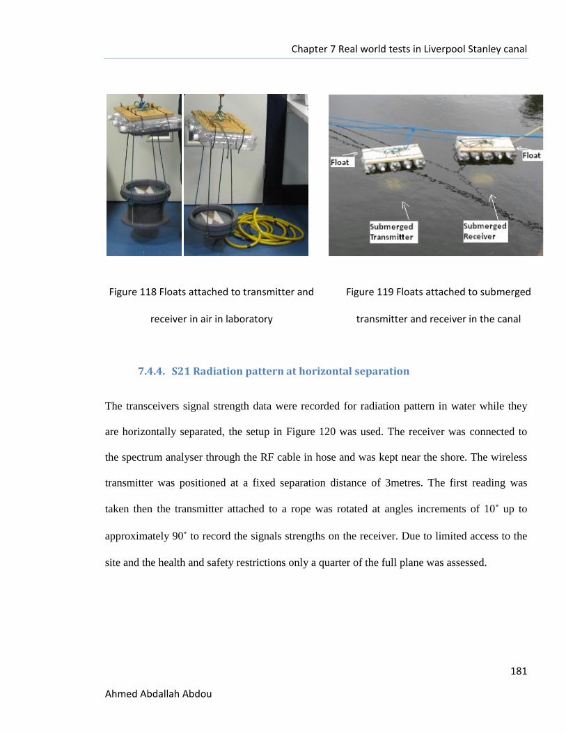
Chapter 7 Real world tests in Liverpool Stanley canal
181
Ahmed Abdallah Abdou
Figure 118 Floats attached to transmitter and
receiver in air in laboratory
Figure 119 Floats attached to submerged
transmitter and receiver in the canal
7.4.4. S21 Radiation pattern at horizontal separation
The transceivers signal strength data were recorded for radiation pattern in water while they
are horizontally separated, the setup in Figure 120 was used. The receiver was connected to
the spectrum analyser through the RF cable in hose and was kept near the shore. The wireless
transmitter was positioned at a fixed separation distance of 3metres. The first reading was
taken then the transmitter attached to a rope was rotated at angles increments of 10˚ up to
approximately 90˚ to record the signals strengths on the receiver. Due to limited access to the
site and the health and safety restrictions only a quarter of the full plane was assessed.

Chapter 7 Real world tests in Liverpool Stanley canal
182
Ahmed Abdallah Abdou
Figure 120 S21 Radiation pattern experiment at horizontal separation in Stanley canal
7.5. Results and discussion
7.5.1. S11 Reflection coefficient in Smith chart
The real parts and Imaginary parts of the antenna’s reflection coefficient while in the water of
the canal were collected from the VNA for frequencies between 100MHz and 800MHz.

Chapter 7 Real world tests in Liverpool Stanley canal
183
Ahmed Abdallah Abdou
However because the 433MHz frequency of interest was in the 400-500MHz region, this
region only was displayed in Figure 121.
Figure 121 Smith chart for the receiver’s antenna in Stanley canal for frequencies
400-500MHz
The 400-500MHz frequency range is close to the centre and the 433MHz marker was one of
the closest on this range. Although after graphical reading on the Smith chart, the next step is
to match for 50ohm impedance (Г=0), however this is more appropriate for narrow band
433MHz
Γ=-1 Γ= 0
Γ= 1
-1
-0.5
0
0.5
1
-1 -0.5 0 0.5 1
Real Г
Imaginary Г

Chapter 7 Real world tests in Liverpool Stanley canal
184
Ahmed Abdallah Abdou
antenna at a given frequency. Maintaining a wide bandwidth to accommodate signal
fluctuations in the water is a requirement as long as the antenna return loss is more than 10dB
(90% of transmission).
7.5.2. Return Loss
Figure 122 S11 Return loss of the receiver’s antenna in Stanley canal
The converted values of real and imaginary reflection coefficient to return loss were plotted in
Figure 122. From this graph a wide bandwidth with a minimum of 10dB RL was seen from
approximately 150MHz up to 800MHz. At 433MHz the RL was -18.05dB and was equivalent
to 98.42% transmission.
4.33E+08 -18.05763079
-50
-45
-40
-35
-30
-25
-20
-15
-10
-5
0
1.00E+08 2.00E+08 3.00E+08 4.00E+08 5.00E+08 6.00E+08 7.00E+08 8.00E+08
S11
(dB
)
Frequencies (MHz)
RL of all frequencies RL at 433MHz
Wide bandwidth

Chapter 7 Real world tests in Liverpool Stanley canal
185
Ahmed Abdallah Abdou
7.5.3. S21 Transmission at horizontal separation
The transceivers were separated every metre for the first 10metres then every 2metres until
30metres. Ten signal strengths readings were collected in microvolts (μV) and averaged by the
spectrum. Those values were then converted in dBm and plotted in Figure 123. At 12m
separation between the transmitter and the receiver, the locks were opened consecutively for
boats passage. This created waves which made the attached transceivers fluctuate. This
phenomenon depicted a real world application where transceivers could be moved from their
original position and therefore the signal strength before and after the opening of the locks was
important.
Figure 123 S21 Transmission of transceivers separated horizontally in the canal water
Figure 123 displays signal strength (S21) experimented for the bow-tie antennas in water in
the canal over a distance of 35m. Two regions were observed, a near-field region up to
-130
-120
-110
-100
-90
-80
-70
-60
-50
-40
-30
0 5 10 15 20 25 30 35
S21
(d
Bm
)
distance (m)
Chapter 7 Real world tests in Liverpool Stanley canal
186
Ahmed Abdallah Abdou
approximately 2m separation distance and a far-field region onwards up to 30m. After that the
signal was recovered any more. In the near-field region, the signal lost 43dB. The far field
losses were expected to attenuate approximately 20dB/m according to the theoretical
calculations in Table 3 for a 433MHz plane wave in water referred to as freshwater. However
in this experiment, the losses were 15dB for 28 metres. This could be explained that the low
signal reached the noise level because of the spectrum analyser sensitivity or the signal had to
travel in lower permittivity material (ground and air) before reaching the submerged antenna.
In the first case, the signal was in the -110dB the far field loss region and transceivers
operating at 433MHz that have sensitivity down to -122dBm could be used to detect such
small signals at such big distances in the water with the bow-tie antenna. In the second case it
would not matter if the signal found other paths than water to reach the receiver as long as it
could be recovered.
With regards to the opening of the locks, the signal changed only 1%. The fact that the
transceivers resisted the waves created by the opening of the locks in the canal provided some
confidence for usage even in windy periods.
7.5.4. S21 Radiation pattern at horizontal separation in Stanley canal
Figure 124 displays the signal strength as radiation pattern on a 360˚ plane of the transceivers
separated horizontally 3metres in the canal. Only up to 90˚ of data was recorded and
represented graphically.

Chapter 7 Real world tests in Liverpool Stanley canal
187
Ahmed Abdallah Abdou
Figure 124 S21 radiation pattern (up to approximately 90˚) at horizontal separation in Stanley
canal
From the quarter plane represented in Figure 124, the highest signal occurred at 0˚ and the
lowest at 90˚. This is in agreement with all the radiation experiment resulted both in air and
water. The shape in between the 0˚ and 90˚ angles followed the shape of the first quarter of
radiation of transceivers in the tank of water at 1000mm separation in Figure 97. Therefore the
radiation patterns of the remaining 3 quarters in the canal were predicted as in Figure 125.
-120
-115
-110
-105
-100
-95
-900
10 2030
40
50
60
70
80
90
100
110
120
130
140150
160170180190200
210220
230
240
250
260
270
280
290
300
310
320
330340
350 360
SignalStrength(dBm)in canalwater3000mmaway
S21 in dBm
Radiation angle in degree

Chapter 7 Real world tests in Liverpool Stanley canal
188
Ahmed Abdallah Abdou
Figure 125 S21 Radiation pattern and predicted at horizontal separation in Stanley canal
The best positioning of the transceivers for communicating under the water of the canal was
when the antennas were 0˚ and 180˚ in line. The worst positioning was at approximately 90˚
and 270˚ with signal strength that gone smaller up to -117dBm.
7.6. Summary
In this chapter, robust waterproof enclosures were designed and prototyped for the
transceivers to be experimented in a real world trial in Liverpool Stanley Canal freshwater.
S11 results shown that the 433MHz air designed and constructed Bow-tie antennas behaved
well even in freshwater. S21 transmissions results proved thriving communication range up to
30metres. This can be used in many applications that apply two way communications. In

Chapter 7 Real world tests in Liverpool Stanley canal
189
Ahmed Abdallah Abdou
Wireless Sensor Networks where an omnidirectional pattern of the sensors is required, a
separation of 5 to 10metres with such low power signal can be realistic to cover a wide area.

Chapter 8 Further Modelling with the Bowtie antenna
190
Ahmed Abdallah Abdou
Chapter 8. Further Modelling with the Bowtie antenna
8.1. Introduction
In chapter 5, the Bowtie antenna modelled to operate at 433MHz in air taking into account the
restrictions of the levelling board of the PCB machine proved its usefulness in water without
matching circuit and therefore the immediate focus was not on optimizing the size of the
antenna. Instead in chapter 6, the focus was more on how to eliminate or reduce the chance of
RF crosstalk from the cables that may act as antennas and could results in false readings in a
two way communication system that was planned for a real life test in the Liverpool Stanley
Canal freshwater as in chapter 7. In this chapter, we altered the bowtie antenna sizes and
modelled the antenna in water with the same conditions as chapter 5. Therefore the arm length
of the antenna was changed while keeping the outer width of the antenna fixed to 91.5mm. In
[103], it is stated that the bandwidth of the bowtie antenna depends on the length of the plate
and that the flare angle and the length of the plate define the lower frequency. Therefore we
monitored the starting low frequency with a minimum of 10dB return loss and the bandwidth
available. In practice, this will allow us to see whether the antenna prototyped in chapter 5
could be optimised and prototyped again in our laboratory or elsewhere. For these, we had two
cases:
Case 1: The levelling board of the PCB machine restricted the size of the antenna
board to a maximum of 210mm length and 120mmwidth. Therefore the maximum arm
length of 101.6mm was reduced in 20mm steps down to 20mm.

Chapter 8 Further Modelling with the Bowtie antenna
191
Ahmed Abdallah Abdou
Case2: There were possibilities to prototype the antenna on a PCB machine with an
antenna board of 350mm length and 120mm width. Therefore the minimum arm length
here was 101.6mm and was increased in 20mm steps up to 160mm.
8.2. Case 1: restricted to an antenna board of 210mm length and 120mm width
8.2.1. Bowtie antenna design alteration and modelling
This first case was a reality because the antenna board size was restricted by the levelling
board of the PCB machine to 210mm length and 120mm width. Therefore we reduced the
bowtie maximum arm length of 101.6mm by approximately 20mm down to 20mm as sketched
in Figure 126. The dimensions of the bowtie antenna after alterations were measured in HFSS
and displayed in Table 6. Reducing the arm length increased the flare angle.
Figure 126 Schematic of Bowtie antenna with reduced arm length from 101.6mm to 20mm
on a 210mm×120mm antenna board
101.6mm 80mm 60mm 40mm 20mm 20mm 40mm 60mm 80mm 101.6mm

Chapter 8 Further Modelling with the Bowtie antenna
192
Ahmed Abdallah Abdou
Table 6 Measured dimensions in HFSS of the Bowtie with reduced arm length from 101.6mm
to 20mm
Board width Sub x(mm)
Board length Sub y(mm)
Outer width(mm)
Hypotenuse (mm)
Angle in degrees
Arm length (mm)
120 210 91.5 110.4 46.07 101.6
120 210 91.5 90.9 56.74 80
120 210 91.5 73.9 71.5 60
120 210 91.5 58.87 94.4 40
120 210 91.5 47.6 130.31 20
8.2.2. Results and discussion
Figure 127 Return Loss (dB) of the Bowtie antenna modelled in water with reduced arm
length from 101.6mm to 20mm
0.00 0.20 0.40 0.60 0.80 1.00Freq [GHz]
-22.50
-20.00
-17.50
-15.00
-12.50
-10.00
-7.50
-5.00
-2.50
0.00
Y1
Return Loss ANSOFT
Curve Info
dB(S(1,1)) 20mm arm length
dB(S(1,1)) 40mm arm length
dB(S(1,1)) 60mm arm length
dB(S(1,1)) 80mm arm length
dB(S(1,1)) 101.6mm arm length
Starting low frequency shift

Chapter 8 Further Modelling with the Bowtie antenna
193
Ahmed Abdallah Abdou
Table 7 Consequences of reduced arm length from 101.6mm to 20mm of the Bowtie antenna
modelled in water
Arm length (mm)
Starting low frequency (GHz)
Bandwidth (GHz)
101.6 0.104 0.9
80 0.139 0.13, 0.67
60 0.189 0.13, 0.18, 0.4
40 0.258 0.11
20 0.368 0.06, 0.09
From Figure 127 and Table 7, reducing the arm length pushed the starting low frequency with
at least 10dB of return loss to higher frequencies. E.g. the bowtie antenna with arm length
101.6mm had a starting low frequency of 104MHz, but when the arm length was reduced to
20mm then the starting low frequency was 368MHz.
As the arm length is reduced, the bandwidth available in water was reduced too. E.g. there was
a large bandwidth (0.9 GHz) available when the arm length was 101.6mm whereas when the
arm length was reduced to 20mm the bandwidth available was divided in two very small ones
(0.06 and 0.09GHz).
In this case 1, reducing the arm length (increasing the flare angle) with fixed outer width
deteriorated the large bandwidth needed in water to cover the frequency shift from air to
water. This will make the antenna not resonating in air at 433MHz and neither in potable nor
in fresh water. Also changes (e.g. temperature, salinity) within the water environment may
result in signal loss. Therefore the reference size was the ideal compared to the others in case 1

Chapter 8 Further Modelling with the Bowtie antenna
194
Ahmed Abdallah Abdou
in potable and freshwater. For saline water, where low frequency was needed to operate in, the
reduction of the arm length did not help.
8.3. Case 2: not restricted to the levelling board length, arm length size could
be increased
8.3.1. Bowtie antenna design optimisation and modelling
The second assumption was that there were possibilities to prototype the antenna on a PCB
machine with approximately double the length of levelling board up to 350mm but keeping the
120mm width unchanged. Therefore the minimum arm length of the bowtie antenna was
101.6mm and was increased in approximately 20mm steps up to 160mm as sketched in
Figure 128. The dimensions of the bowtie antenna after alterations were measured in HFSS
and displayed in Table 8. Increasing the arm length reduced the flare angle.
Figure 128 Schematic of Bowtie antenna with increased arm length from 101.6mm to 160mm
on a 350×120mm antenna board
101.6mm
140 120 140 160mm 101.6mm 120 160mm 101.6mm 120 140 160mm 101.6mm 120 160mm 101.6mm
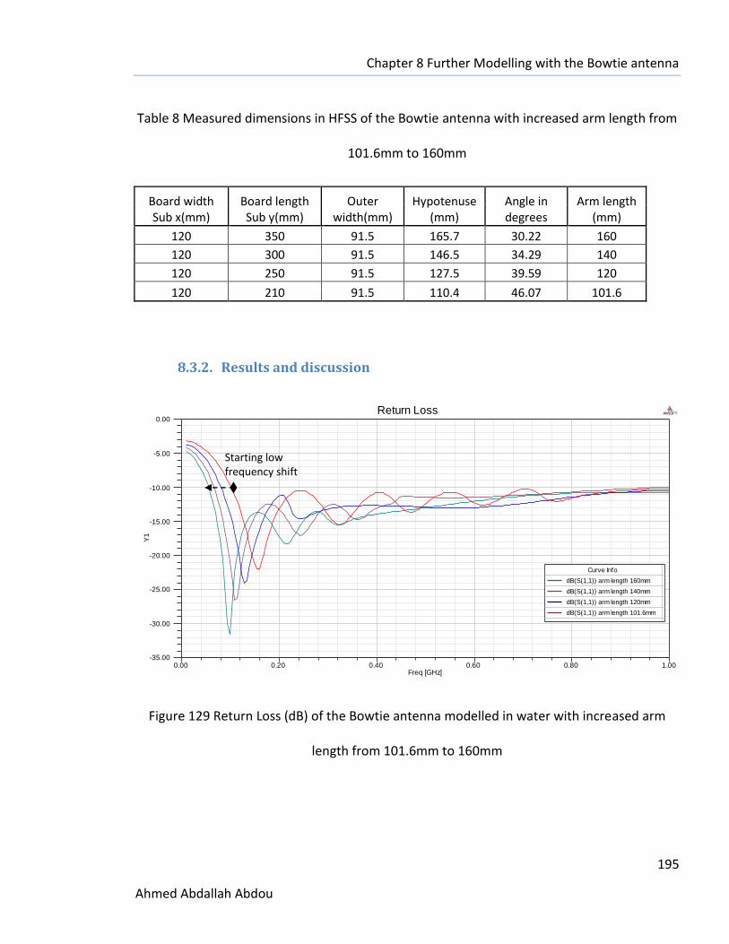
Chapter 8 Further Modelling with the Bowtie antenna
195
Ahmed Abdallah Abdou
Table 8 Measured dimensions in HFSS of the Bowtie antenna with increased arm length from
101.6mm to 160mm
Board width Sub x(mm)
Board length Sub y(mm)
Outer width(mm)
Hypotenuse (mm)
Angle in degrees
Arm length (mm)
120 350 91.5 165.7 30.22 160
120 300 91.5 146.5 34.29 140
120 250 91.5 127.5 39.59 120
120 210 91.5 110.4 46.07 101.6
8.3.2. Results and discussion
Figure 129 Return Loss (dB) of the Bowtie antenna modelled in water with increased arm
length from 101.6mm to 160mm
0.00 0.20 0.40 0.60 0.80 1.00Freq [GHz]
-35.00
-30.00
-25.00
-20.00
-15.00
-10.00
-5.00
0.00
Y1
Return Loss ANSOFT
Curve Info
dB(S(1,1)) arm length 160mm
dB(S(1,1)) arm length 140mm
dB(S(1,1)) arm length 120mm
dB(S(1,1)) arm length 101.6mm
Starting low frequency shift

Chapter 8 Further Modelling with the Bowtie antenna
196
Ahmed Abdallah Abdou
Table 9 Consequences of increased arm length from 101.6mm to 180mm of the Bowtie
antenna modelled in water
Arm length (mm)
Starting low frequency (GHz)
Bandwidth (GHz)
160 0.056 0.94
140 0.067 0.85
120 0.082 0.9
101.6 0.104 0.9
From Figure 129 and Table 9, increasing the arm length pushed the starting low frequency
with at least 10dB of return loss to lower frequencies. E.g. the bowtie antenna with arm length
101.6mm had a starting low frequency of 104MHz, but when the arm length was increased to
160mm then the starting low frequency was 56MHz.
The large bandwidth (≈0.9GHz) obtained with 101.6mm arm length was maintained at every
increased arm length.
In this case 2, increasing the arm length (reducing the flare angle) with fixed outer width
maintained the large bandwidth needed in water to cover the frequency shift from air to water.
This is making the antenna resonates in air at 433MHz as well as in potable and fresh water.
Also changes (e.g. temperature, salinity) within environments will not affect the signal.
Therefore the reference size was ideal compared to the others in case 2 only in potable and
fresh water. For saline water, where low frequency was needed to operate in, the increase of
the arm length could help.

Chapter 8 Further Modelling with the Bowtie antenna
197
Ahmed Abdallah Abdou
In all cases, as from the theory of the Bowtie antenna referenced earlier, the bandwidth of the
bowtie antenna is dependent on the length of the antenna board. The flare angle and the length
of the antenna board defined the starting lower frequency.
8.4. Summary
In this chapter, the Bowtie antenna prototyped in chapter 5 and tested in the canal in chapter 7
was subjected to further modelling in water. This consisted of altering the sizes of the antenna.
Two cases were presented. On the first case, the length of the antenna board was restricted to
the length of the PCB levelling board. By changing the size of the antenna in this case, the
modelling resulted on a reduction of the large bandwidth and a shift of the starting low
frequency to higher frequencies which are both unwanted. The sizes of our prototyped antenna
have shown that the antenna is optimised in potable and freshwater. However when the length
of the antenna board was extended, the modelling resulted in a large bandwidth maintained
and the shift of the starting low frequency to lower frequencies which predicted that the
antenna will also be able to operate in high salinity water (seawater).

Chapter 9 Conclusion
198
Ahmed Abdallah Abdou
Chapter 9. Conclusion
Although the challenges in water environment are becoming more alarming, industrial and
environmental bodies are still relying on traditional and periodic methods in assessing water
health. As technology is evolving, it is providing solutions to many problems. Only some of
the environmental agencies and water industries in developed countries have made use of
technology with the revolution of sensors technology and real time systems. In countries with
financial resource shortage, the cost of these systems makes it almost impossible to acquire
them. Therefore globally there has been a huge need for scientists and technologists to find
new and cheap alternatives capable of replacing conventional and costly ways for assessing
water environment in real time. We have explored State of the art water communications and
found that in many applications, acoustic and optical traditional ways of communicating
underwater between sensor nodes have underperformed and were found unreliable. We have
proposed a breakthrough in underwater communication. This is by using wireless sensor
network communicating through radio and microwaves, a technology that has excelled in
over-the-air applications. This has driven us to aim to investigate short range Electromagnetic
wave communication utilising a sensor network platform. In order to achieve this aim we have
set objectives. The first objective consists of investigating the feasibility of radio frequency
and microwaves communication underwater using the unlicensed ISM band. The second
objective consists of testing the feasibility of using commercial over the air transceivers in
water to sense its health. The third objective is to design, simulate and test an antenna to
operate efficiently in water. The fourth objective is about investigating the feasibility of

Chapter 9 Conclusion
199
Ahmed Abdallah Abdou
forming a WSN to operate in the water column. The first three objectives are the most critical
as the frequency and the antenna are interrelated and the fact that this has to be in water makes
them very challenging however tests with commercial over-the-air wireless transceivers in
water can give a preliminary experimental validation to the first objective. Unlocking these
objectives will answer most of the research and will lead to the last objective set, because the
suitable antenna for the appropriate frequency is key to successful transfer of modulated
carrier signal between the sensor nodes forming the WSN especially in a medium like water.
In order to predict the appropriate frequency to operate in water, it was vital to understand
how electromagnetic waves propagate. So a review of the theory of electromagnetic wave
propagation was undertaken. A study of the effects of the permittivity and the salinity of water
on absorption was carried out. This showed that lower frequencies suffered less absorption.
For potable and freshwater, however the losses up to around 600MHz, still allowed realistic
transmission up to a few metres, and suggested 433MHz and 6.7MHz for communication. For
saline water, the absorption is considerably higher but it was concluded that the 6.7 MHz ISM
band might still be practical. This covered the first objective, which consisted of investigating
the feasibility of radio frequency and microwaves communication underwater using the
unlicensed ISM band. With most commercial transceivers for sensor nodes operating at
2.4GHz ISM, it was necessary, through experimentation, to show the limitations of this
frequency. The theoretical model predicted high attenuation in the 2.4GHz ISM band and this
has been validated in the laboratory tank experiments using a commercial low powered
wireless transceiver with the loss of temperature sensing signal at 200mm in section 3.6.1.1.
This covered the second objective consisting of testing the feasibility of using commercially

Chapter 9 Conclusion
200
Ahmed Abdallah Abdou
available over-the-air wireless transceivers in water to sense its health. The communication
range achieved was limited because of the highly attenuated 2.4GHz frequency of the
transceiver and the unsuitable antenna for water. Therefore this band that provides many
advantages including high data rate, availability in complete kits, was recommended more
favourable in proximity communications for applications requiring a higher data rate (i.e.
Automated Underwater Vehicles collecting data from an underwater node where acoustic and
optical are not viable options) than in UWSN. Further Experiments in the tank validated that
the 433MHz and 6.7MHz could travel further in potable water and the antenna has a crucial
role in signal transmission and reception which require further investigation. Apart from the
theoretical prediction of the usefulness of 433MHz in potable and freshwater, we have
operated in this band because it offers many advantages over the 6.7MHz including the higher
data rate needed for more frequent data sampling and fast data download, off the shelf
transceiver availability and smaller wavelength size to construct an antenna. The choice of the
433MHz frequency for our sensor node which resulted from detailed theoretical and
experimental investigation provided in chapter 3, covers the first two objectives and makes
way to the third objective to design and simulate an antenna to operate efficiently in water.
However the size of the tank limited the experimental verification of this frequency to
communicate up to its maximum distance for sensor nodes separation that will form the
network.
In chapter 4, we have recalled the theory to construct an antenna to operate in air or in water.
Traditional antennas made of copper wire were made for the approved 433MHz frequency and
tested in the tank of the laboratory. The popular loop antenna outperformed and therefore was
Chapter 9 Conclusion
201
Ahmed Abdallah Abdou
subjected to a modelling stage. This consisted of designing and analysing the antenna
behaviour in HFSS in water and air environment. Analyses examined include the return loss
and the bandwidth available, the impedance and the radiation pattern of the antenna. This has
shown that the antenna does not have any bandwidth in air or in water even when the size is
optimised. Although the size of the loop to operate in water has been determined from the
theory to take into account the water reduction factor, the impedance of the antenna in water
and in air is mismatched even when its size is optimised for resonance. This meant that
without matching circuit, communication range required for the UWSN would not be achieved
if we choose any traditional narrowband antenna including the loop and therefore bespoke
antenna must be sought in order to meet the objective. However antenna with matching circuit
will suffer from reduction of signal strength or complete signal loss in varying underwater
parameters including salinity and temperature. Although this chapter does not meet the second
objective set, it has allowed us to specify in chapter 5 the criteria needed on the antenna in
order to operate in water efficiently without any matching means. To select an antenna for
wireless sensor network that could work in air as well as in water, the focus has been on
selecting an antenna that has a broad bandwidth, an omnidirectional radiation pattern but also
an antenna that can be prototyped for practical validation tests. The planar version of the
broadband finite biconical antenna is the Bowtie which can be printed on a dielectric substrate,
and this is selected and investigated. The antenna is modelled in air at 433MHz and in
0.02S/m water in HFSS. Although the simulation results in air shown a limited bandwidth, in
water they show an ultra-broadband behaviour that is needed. The impedance has shown that
the matched antenna in air was close to a matched antenna in potable and freshwater. The
Chapter 9 Conclusion
202
Ahmed Abdallah Abdou
antenna has an omnidirectional radiation pattern in air and maintains it in water. This validates
the first two selection criteria and proceeds to the third criteria referring to ease of prototyping
for practical validation of the antenna in water. The antenna is then successfully prototyped on
PCB and waterproofed for underwater tests. The S11 results of the experiments demonstrate
that the Bow-tie antenna that is designed and constructed for air can be used in water without a
matching circuit. It is understood that this is first time that an antenna designed to operate in
air at 433MHz has been shown to operate in water without any matching. The S11 results of
the simulated 433MHz Bowtie antenna in air and in water were in good agreement with
experimented ones. This implies a recommendation for HFSS in modelling the behaviour of
the antenna in liquids including water. However there has been a limitation on analysing the
signal transmission S21 between two antennas in an open water environment. Further
experiments have shown the Bowtie antenna immunity towards temperature change. This
attribute is linked to its broadband characteristic in water and is needed. Designing, simulating
and testing the 433MHz Bowtie antenna which resulted in its efficient operation in water has
led to demonstrate for the first time the application of bowtie antenna and specifically our
433MHz bowtie antenna in potable and freshwater. This covers the third objective which has
been the crucial part of the research and consisted of designing, simulating and testing an
antenna to operate efficiently in water. The first and the third objectives form the
communication device which is an important component out of the five main components of
the sensor nodes explained in section 2.4.3.1. The remaining four components could be off-
the-shelf components connected to our communication device.

Chapter 9 Conclusion
203
Ahmed Abdallah Abdou
As this sensor node is going to operate in a network, our communication device had to be able
to generate its own carrier signal for transmission to form the physical layer of the network.
Also to validate the first and the third objectives against erroneous results that may arise from
RF cables crosstalk during experiments in water, the carrier signal had to be generated from a
wireless battery powered RF source. We have therefore designed and prototyped a battery and
low powered 433MHz carrier signal generator. The electronic set is waterproofed and tested in
a laboratory tank with the Bowtie antenna for S21 signal transmission. Experimental results
confirm the suitability of the bowtie antenna in a true wireless sensor node and successful
reception of the 433MHz carrier signal transmitted through the antenna for up to half a meter.
This distance was limited because of the tank size however analysis of the signal showed a far
field region predicting higher communication range. The fourth objective consisted of
investigating the feasibility of forming a WSN to operate in the water column. In order to form
a network, sensor nodes had to be able to communicate at least for a distance of 3 to 5metres,
as mentioned in the design specification. Therefore we have subjected our communication
device to an experiment in Liverpool Stanley Canal Freshwater. For this we have designed
robust waterproof enclosures for the transceivers in SolidWorks and prototyped. The S11
results have shown that our bowtie antenna behave well even in freshwater. The S21
transmissions results have proved a thriving communication range up to 30metres. This range
has broadened the applications of our communication device with the Bowtie antenna for two
way communication systems operating in potable and freshwaters. In WSN, an
omnidirectional pattern of the sensors is required; therefore we recommend a separation of 5
to 10metres with such low power signal to cover a wide area. The fourth objective is therefore

Chapter 9 Conclusion
204
Ahmed Abdallah Abdou
met in chapter 7 and the findings confirm that our communication system combined with the
remaining 3 off the shelf components (memory, controller, water health sensor) will form a
wireless sensor node. Duplicating this node will constitute the WSN needed to cover and
monitor the health of a wide underwater zone.
The contribution to knowledge is the experimental demonstration of reliable communication at
433MHz using a broadband antenna which unlocks the potential of underwater WSN
applications, including applications in water quality measurement, using radio communication.
Further modelling in water on the 433MHz Bowtie antenna prototyped and tested in the canal
is done. This consisted of altering the sizes of the antenna. Two cases were presented. On the
first case, the length of the antenna board was restricted to the length of the PCB levelling
board. By changing the size of the antenna in this case, the modelling resulted in a reduction
of the large bandwidth and a shift of the starting low frequency to higher frequencies which
are both unwanted for water communication. The sizes of our prototyped antenna have shown
that the antenna was optimised in potable and freshwater. However when the length of the
antenna board was extended, the modelling resulted in a large bandwidth maintained and shift
of the starting low frequency to lower frequencies which predict that the antenna could also be
able to operate in high salinity water (seawater). These findings are unique and open up a huge
area of investigation which could be applied in a wide range of seawater applications
including seawater environmental monitoring, commercial subsea applications, defence and
military applications etc.

Chapter 10 Future work
205
Ahmed Abdallah Abdou
Chapter 10. Future work
The Bowtie antenna could be attached to an off the shelf board transceiving at 433MHz which
will replace the carrier signal generator and send a modulated signal. This will form the
complete communication system. Different types of modulation could be studied in water.
Depending on the application, single or multi parameters sensor that can measure properties
like pH, Dissolved Oxygen, turbidity, chlorophyll a, temperature, pressure, salinity,
conductivity can be attached to the underwater communication system. Those related to the
application will be studied; the condition and parameters, under which maximum reliability
and sensitivity will occur, will be considered.
The communication system and the sensor could be duplicated to form a network of sensor
nodes. This could monitor physical variables such as water temperature and pressure as well
as variables such as conductivity, turbidity and certain pollutants. The network could track
accidental release of pollutants flowing in water from land. It could monitor and model the
behaviour of underwater ecosystems. The network could be used to identify or monitor in real
time deliberate pollution or even potential terrorist attack to water reservoirs that could
contaminate water supply and put in danger public health. A map of the water reservoir with
areas of contamination could be generated for the authorities to take immediate action like
stopping, the supply of contaminated water from getting to the public.
Chapter 10 Future work
206
Ahmed Abdallah Abdou
The network of underwater sensor nodes could be modelled in platforms such as Opnet or Ns-
2 where parameters of the network including power, quantity of service (throughput), quality
of service (QoS), mobility, protocols, etc can be studied.
Further modelling on the Bowtie antennas could be done to find the optimised size to operate
efficiently in saline water. This could then be prototyped and tested in seawater. The Bowtie
antenna could be re-engineered to suit saline water applications.

0 References
207
Ahmed Abdallah Abdou
References
[1] A. Al-Shammaa, A. Shaw, and S. Saman, “Propagation of Electromagnetic Waves at MHz Frequencies Through Seawater,” IEEE Transactions on Antennas and Propagation, vol. 52, no. 11, pp. 2843–2849, Nov. 2004.
[2] Y. Huang and K. Boyle, Antennas from theory to practice. John Wiley & Sons, Ltd, 2008.
[3] T. Apps, “Apps Laboratories,” salinity, 2012. [Online]. Available: http://www.appslabs.com.au/salinity.htm. [Accessed: 20-Jan-2012].
[4] R. Weiner and R. Matthews, Environmental Engineering, Fourth Edi. 2003.
[5] Environment Agency, “The unseen threat to water quality,” 2007.
[6] Betancourt, V. Hemmen, Greco, and Kenyon, “International Convention for the Prevention of Pollution of the Sea by Oil,” International Conventions, 1954. [Online]. Available: http://www.admiraltylawguide.com/conven/oilpol1954.html. [Accessed: 05-Apr-2012].
[7] F. Bernardini, “UNECE Convention on the Protection and Use of Transboundary Watercourses and International Lakes,” 1992.
[8] European Commission, “Urban Waste Water Directive Overview,” Environment, 1991. [Online]. Available: http://ec.europa.eu/environment/water/water-urbanwaste/index_en.html. [Accessed: 05-Apr-2012].
[9] European Commission, “Implementation of nitrates Directive 91/676/EEC,” Environment, 1991. .
[10] European Commission, “Drinking water directive 98/83/EC,” Drinking water legislation, 1998. [Online]. Available: http://ec.europa.eu/environment/water/water-drink/legislation_en.html. [Accessed: 05-Apr-2012].
[11] European Commission, “The EU Water Framework Directive,” 2000. [Online]. Available: http://ec.europa.eu/environment/water/water-framework/index_en.html. [Accessed: 05-Apr-2012].
[12] N. F. Gray, Water technology: an introduction for environmental scientists and engineers, Second edi. Dublin: Elsevier Butterworth-Heinemann, 2005, p. 127.

0 References
208
Ahmed Abdallah Abdou
[13] European Commission, “Environmental liability,” Liability, 2004. [Online]. Available: http://ec.europa.eu/environment/legal/liability/. [Accessed: 05-Apr-2012].
[14] European Commission, “Bathing water directive 2006/7/EC,” Bathing water quality, 2006. [Online]. Available: http://ec.europa.eu/environment/water/water-bathing/. [Accessed: 05-Apr-2012].
[15] European Union, “DIRECTIVE 2008/56/EC OF THE EUROPEAN PARLIAMENT AND OF THE COUNCIL,” Official Journal of the European Union, no. L 164 2008 EC, pp. 19–40, 2008.
[16] HMSO, The Water Resources Act 1991 (Amendment) (England and Wales) Regulations 2009 No. 3104, vol. 1991, no. 3104. WATER RESOURCES , ENGLAND AND WALES, 2009.
[17] HMSO, “Water Industry Act 1991,” Legislation, 1991. [Online]. Available: http://www.legislation.gov.uk/ukpga/1991/56/contents. [Accessed: 05-Apr-2012].
[18] Department for Environment Food and Rural Affairs, “The Environmental Damage (Prevention and Remediation) Regulations 2009,” London, 2009.
[19] HMSO, “Marine and Coastal Access Act 2009,” Legislation, 2009. [Online]. Available: http://www.legislation.gov.uk/ukpga/2009/23/contents. [Accessed: 05-Apr-2012].
[20] Environment Agency, “Managing and improving the water environment,” 2011. .
[21] Department for Environment Food and Rural Affairs, “The Natural Choice: securing the value of nature,” London, 2011.
[22] Department for Environment Food and Rural Affairs, “Water for Life,” London, 2011.
[23] Department for Environment Food and Rural Affairs, “Tackling water pollution from the urban environment Consultation on a strategy to address diffuse water pollution from the built environment,” London, 2012.
[24] Department for Environment Food and Rural Affairs, “Summary of responses to the consultation on ‘ Tackling water pollution from the urban environment ’,” London, 2013.
[25] Government, “Improving water quality,” Policy, 2014. [Online]. Available: https://www.gov.uk/government/policies/improving-water-quality.

0 References
209
Ahmed Abdallah Abdou
[26] European Union, “Council Directive 98/83/EC of the 3rd November 1998 on the quality of water intended for human consumption,” Official Journal of the European Communities, vol. L330/32, no. 5.12.98, 1998.
[27] Environment Agency, “The Microbiology of Drinking Water (2002) - Part 1 - Water Quality and Public Health,” 2002.
[28] Environment Agency, “The Microbiology of Drinking Water (2010) - Part 2 – Practices and procedures for sampling Methods for the Examination of Waters and Associated Materials,” 2010.
[29] Wattera, “Water quality equipment,” Innovations in Water Monitoring, 2013. [Online]. Available: http://www.waterra-in-situ.com/pages/category/water_quality.asp?gclid=CP6R1NGMursCFQHHtAodnW0Aaw. [Accessed: 18-Dec-2013].
[30] EMS, “Environmental Monitoring Solutions,” Water quality, 2013. [Online]. Available: http://www.em-solutions.co.uk/products/water_monitoring. [Accessed: 18-Dec-2013].
[31] Cole-Parmer Instrument Company Limited, “Global Water Dissolved Oxygen,” Global Water DO Sensor, 2013. [Online]. Available: http://www.coleparmer.co.uk/Product/Global_Water_Dissolved_Oxygen_Sensor/UY-99243-38?referred_id=3482&gclid=CJuos6ucursCFdLItAodyXEAKQ. [Accessed: 18-Dec-2013].
[32] YSI/Xylem, “YSI Integrated Systems & Services,” Water Quality Monitoring System, 2013. [Online]. Available: http://www.ysisystems.com/floating-platform-selector.php. [Accessed: 18-Dec-2013].
[33] YSI, “Real-time Water Quality Data from Dubai Creek,” YSI Environmental, 2013. [Online]. Available: http://www.ysi.com/media/pdfs/A526-Dubai-Municipality-Utilizes-Real-time-Water-Quality-Monitoring-Instruments.pdf. [Accessed: 18-Dec-2013].
[34] YSI, “Water Quality Is Key To The Success Of Cardiff Bay,” Water Today, pp. 12–15, 2011.
[35] N. Mohamed, I. Jawhar, J. Al-Jaroodi, and L. Zhang, “Monitoring Underwater PIpelines Using Sensor Networks,” 2010 IEEE 12th International Conference on High Performance Computing and Communications, pp. 346–353, Sep. 2010.

0 References
210
Ahmed Abdallah Abdou
[36] S.Sato, H.Yamamoto, and Y. Okuyama, “Pipeline built-in electric power generating set,” 4740711, 1988.
[37] N. Mohamed, I. Jawhar, J. Al-Jaroodi, and L. Zhang, “Sensor network architectures for monitoring underwater pipelines.,” Sensors (Basel, Switzerland), vol. 11, no. 11, pp. 10738–64, Jan. 2011.
[38] I. F. Akyildiz, D. Pompili, and T. Melodia, “Underwater acoustic sensor networks: research challenges,” Ad Hoc Networks (Elsevier), vol. 3, no. 3, pp. 257–279, May 2005.
[39] Teledyne RESON, “Hydrophones,” 2012. [Online]. Available: www.teledyne-reson.com/products/hydrophones/. [Accessed: 05-Feb-2012].
[40] University of Rhode Island, “Acoustic monitoring,” Discovery of Sound in the Sea, 2012. [Online]. Available: http://www.dosits.org/animals/effectsofsound/howdoyoumeasureamarinemammalsreactiontosound/acousticmonitoring/. [Accessed: 05-Feb-2012].
[41] W. Au, The Sonar of Dolphins. New York: Springer-Verlag, 1993.
[42] M. Stojanovic, “On the relationship between capacity and distance in an underwater acoustic communication channel,” ACM SIGMOBILE Mobile Computing and Communications Review, vol. 11, no. 4, p. 34, Oct. 2007.
[43] L. Berkhovskikh and Y. Lysanov, Fundamentals of Ocean Acoustics. New York: Springer, 1982.
[44] R. Coates, Underwater Acoustic Systems. New York: Wiley, 1989.
[45] J. Krautkramer and H. Krautkramer, Ultrasonic testing of materials. Heidelberg, Germany: Springer, 1990.
[46] I. Vasilescu, K. Kotay, D. Rus, M. Dundabin, and P. Corke, “Data collection, storage, and retrieval with an underwater sensor network,” Proceedings of the 3rd international conference on Embedded networked sensor systems - SenSys’05. ACM Press, New York, New York, USA, p. 154, 2005.
[47] Y. Tsuchida, N. Hama, and M. Takahata, “An optical telemetry system for underwater recording of electromyogram and neuronal activity from non-tethered crayfish.,” Journal of neuroscience methods, vol. 137, no. 1, pp. 103–9, Aug. 2004.

0 References
211
Ahmed Abdallah Abdou
[48] J. Smart., “Underwater optical communications systems part 1: variability of water optical parameters,” in IEEE Military Communications Conference. MILCOM, 2005, pp. 1140–1146.
[49] J. A. Simpson, “A 1 Mbps Underwater Communications System using LEDs and Photodiodes with Signal Processing Capability,” North Carolina State University, Raleigh, NC, 2007.
[50] M. Doniec, I. Vasilescu, M. Chitre, C. Detweiler, M. Hoffmann-kuhnt, and D. Rus, “AquaOptical : A Lightweight Device for High-rate Long-range Underwater Point-to-Point Communication,” in OCEANS 2009, MTS/IEEE Biloxi - Marine Technology for Our Future: Global and Local Challenges, 2009, pp. 1–6.
[51] W. Cox, “A 1 Mbps Underwater Communication System Using a 405 nm Laser Diode and Photomultiplier Tube,” North Carolina State University, Raleigh, NC, NC, 2007.
[52] SAPHOTONICS, “No Title,” Technologies, 2012. [Online]. Available: http://www.saphotonics.com/high-bandwidth-optical-communications/underwater/. [Accessed: 04-Dec-2012].
[53] F. Hanson and S. Radic, “High bandwidth underwater optical communication,” Applied Optics, vol. 47, no. 2, pp. 277–283, 2008.
[54] L. J. Johnson, R. J. Green, and M. S. Leeson, “Underwater optical wireless communications : depth dependent variations in attenuation,” Applied Optics, vol. 52, no. 33, pp. 7867–7873, 2013.
[55] M. A. A. Ali, “Analyzing of Short Range Underwater Optical Wireless Communications Link,” INTERNATIONAL JOURNAL OF ELECTRONICS & COMMUNICATION TECHNOLOGY, vol. 4, no. 3, pp. 125–132, 2013.
[56] B. E. A. Saleh and M. C. Teich, Fundamentals of Photonics, Second. Wiley Interscience, 2007.
[57] J. R. Apel, Principles of Ocean Physics. Academic Press, 1987.
[58] M. Lanzagorta, Underwater Communications, VirginiaTe. Virginia: Morgan & Claypool Publishers, 2013, pp. 32–42.
[59] J. A. Willoughby and P. D. Lowell, “Development of loop aerial for submarine radio communication,” American Physics Society, vol. 14, no. 2, p. 193, 1919.

0 References
212
Ahmed Abdallah Abdou
[60] A. Shaw, A. I. Al-Shammaa, S. R. Wylie, and D. Toal, “Experimental Investigations of Electromagnetic Wave Propagation in Seawater,” in 2006 European Microwave Conference, 2006, no. September, pp. 572–575.
[61] J. H. Goh, A. Shaw, and A. I. Al-Shammaa, “Underwater wireless communication system,” Journal of Physics: Conference Series, vol. 178, p. 012029, Jul. 2009.
[62] A. A. Abdou, A. Shaw, J. Cullen, S. Wylie, A. Mason, and A. Al-Shamma, “A Review of Underwater EM Wave Propagation to Investigate the Development of a Through Water WSN,” in 6th Built Environment And Natural Environment, 2011, pp. 1–6.
[63] A. A. Abdou, A. Shaw, A. Mason, A. Al-Shamma, J. Cullen, and S. Wylie, “Electromagnetic (EM) Wave Propagation for the Development of an Underwater Wireless Sensor Network (WSN),” in Sensors, 2011 IEEE, 2011, no. 1, pp. 1571 – 1574.
[64] WFS Technologies Ltd, “Subsea Wireless Solutions,” Subsea Wireless Technologies, 2013. [Online]. Available: http://www.wfs-tech.com. [Accessed: 05-Dec-2011].
[65] W. Merrill, K. Sohrabi, L. Girod, J. Elson, F. Newberg, and W. Kaiser, “Open Standard Development Platforms for Distributed Sensor Networks,” in Unattended Ground Sensor Technologies and Applications IV, 2002, pp. pp.327–337.
[66] A. Mason, A. Shaw, and A. I. Al-Shammaa, “Inventory Management in the packaged Gas Industry Using Wireless Sensor Networks,” in Advances in Wireless Sensors and Sensor Networks, S. C. Mukhopadhyay and H. Leung, Eds. Springer, 2010, pp. 75–100.
[67] L. E. Cordova-Lopez, A. Mason, J. D. Cullen, A. Shaw, and A. I. Al-Shammaa, “Online vehicle and atmospheric pollution monitoring using GIS and wireless sensor networks,” Journal of Physics: Conference Series, vol. 76, p. 012019, Jul. 2007.
[68] E. Stuntebeck, D. Pompili, and T. Melodia, “Wireless underground sensor networks using commodity terrestrial motes,” 2006 2nd IEEE Workshop on Wireless Mesh Networks, pp. 112–114, 2006.
[69] S. Pandya, J. Engel, J. Chen, Z. Fan, and C. Liu, “CORAL: Miniature Acoustic Communication Subsystem Architecture for Underwater Wireless Sensor Networks,” in The 4th IEEE International Conference on Sensors, 2005.
[70] T.-H. Won and S.-J. Park, “Design and implementation of an omni-directional underwater acoustic micro-modem based on a low-power micro-controller unit.,” Sensors (Basel, Switzerland), vol. 12, no. 2, pp. 2309–23, Jan. 2012.

0 References
213
Ahmed Abdallah Abdou
[71] M. Dunbabin, P. Corke, I. Vasilescu, and D. Rus, “Data muling over underwater wireless sensor networks using an autonomous underwater vehicle,” in Proceedings of the 2006 IEEE International Conference on Robotics and Automation, 2006, no. May, pp. 2091–2098.
[72] D. Anguita, D. Brizzolara, and G. Parodi, “Building an Underwater Wireless Sensor Network Based on Optical: Communication: Research Challenges and Current Results,” 2009 Third International Conference on Sensor Technologies and Applications, pp. 476–479, Jun. 2009.
[73] R. M. Hagem, D. V. Thiel, S. G. O’Keefe, and T. Fickenscher, “THE EFFECT OF AIR BUBBLES ON AN UNDERWATER OPTICAL COMMUNICATIONS SYSTEM FOR WIRELESS SENSOR NETWORK,” Microwave and Optical Technology Letters, vol. 54, no. 3, pp. 729–732, 2012.
[74] J. Lloret, “Underwater sensor nodes and networks.,” Sensors (Basel, Switzerland), vol. 13, no. 9, pp. 11782–96, Jan. 2013.
[75] A. Elrashidi, A. Elleithy, M. Albogame, and K. Elleithy, “Underwater Wireless Sensor Network Communication Using Electromagnetic Waves at Resonance Frequency 2 . 4 GHz,” in CNS ’12 Proceedings of the 15th Communications and Networking Simulation Symposium, 2012.
[76] J. Lloret, S. Sendra, M. Ardid, and J. J. P. C. Rodrigues, “Underwater wireless sensor communications in the 2.4 GHz ISM frequency band.,” Sensors (Basel, Switzerland), vol. 12, no. 4, pp. 4237–64, Jan. 2012.
[77] H. Karl and A. Willing, Protocols and Architectures for Wireless Sensor Networks. John Wiley & Sons, Ltd, 2005, p. 18.
[78] D. K. Cheng, Field and Wave Electromagnetics, Second. Addisson Wesley Publishing Company, 1989, p. 367.
[79] S. J. Orfanidis, “Electromagnetic Waves and Antennas,” 2008. [Online]. Available: http://www.ece.rutgers.edu/~orfanidi/ewa/. [Accessed: 09-Dec-2013].
[80] Ofcom, “Spectrum,” The Communications Market 2005-Overview, 2005. [Online]. Available: http://stakeholders.ofcom.org.uk/market-data-research/market-data/communications-market-reports/cm05/overview05/spectrum/. [Accessed: 06-Dec-2013].

0 References
214
Ahmed Abdallah Abdou
[81] ITU, “Frequency allocations map,” Article 5 Frequency Allocation, 2009. [Online]. Available: http://life.itu.int/radioclub/image/regmap.gif. [Accessed: 06-Dec-2013].
[82] M. N. O. Sadiku, Elements of Electromagnetics, Third. Oxford University Press, 2001, pp. 417–422.
[83] R. W. P. King and G. S. Smith, Antennas in Matter. Cambridge, MA: MIT Press, 1981.
[84] D. Lide, CRC Handbook of Chemistry and Physics, 2010th ed. CRC Press/ Taylor and Francis, 2010.
[85] P. Debye, Polar Molecules. New York: Chemical Catalog Company, 1929.
[86] B. D. Thomas, T. G. Thomson, and C. L. Utterback, “The electrical conductivity of sea water,” Const. Int. Explor. Mer, vol. 9, no. 1934, pp. 28–35, 1934.
[87] R. A. Cox, “The physical properties of seawater,” in Chemical Oceanography, vol. 1, J. P. Riley and G. Skirrow, Eds. New York: Academic Press, 1965.
[88] L. A. Klein and C. . Swift, “An improved model for the dielectric constant of seawater at microwave frequencies,” IEEE J. Oceanic Eng., pp. 104–111, 1977.
[89] C. Guillou, W. Elisson, L. Eymard, K. Lamkaouchi, C. Pringent, G. Delbos, G. Balana, and S. A. Boubakara, “Impact of new permittivity measurements on sea surface emissivity modelling microwaves,” Radio Science, vol. 33, no. 3, pp. 649–667, 1998.
[90] J. R. Wang, “A comparison of the MIR-E stimated and Model-Calculated fresh water surface emissivities at 89, 150 and 220 GHz,” in IEEE Transactions on Geoscience and Remote Sensing, 2002, pp. 1356–1365.
[91] T. Meissner and F. J. Wentz, “The complex dielectric constant of pure and sea water from microwave satellite observations,” IEEE Transactions on Geoscience and Remote Sensing, vol. 42, no. 9, pp. 1836–1849, Sep. 2004.
[92] A. P. Stogryn, H. T. Bull, K. Rubayi, and S. Iravanchy, “THE MICROWAVE DIELECTRIC PROPERTIES OF SEA AND FRESH WATER,” Azusa, 1995.
[93] Würth Elektronik eiSos GmbH & Co KG, “Chip-Antenna WE-MCA part no 7488910245,” Specification for release, 2004. [Online]. Available: http://katalog.we-online.de/pbs/datasheet/7488910245.pdf. [Accessed: 25-Mar-2011].

0 References
215
Ahmed Abdallah Abdou
[94] A. A. Abdou, A. Shaw, A. Mason, A. Al-Shamma, S. Wylie, and J. Cullen, “Wireless Sensor Network for Underwater Communication,” in Wireless Sensor Systems, 2012, pp. 3–8.
[95] Texas Instruments, “Wireless Sensor Monitor Using the eZ430-RF2500 (SLAA378D),” Dallas, 2011.
[96] Texas Instruments, “Project collateral and source code (SLAC139),” 2007. [Online]. Available: http://www.ti.com/lit/zip/slac139. [Accessed: 10-Nov-2011].
[97] Texas Instruments, “CC2500 datasheet (SWRS040C),” Dallas, 2007.
[98] Futurlec, “Radio modules,” Boards, 2012. [Online]. Available: http://www.futurlec.com/Radio-433MHZ.shtml. [Accessed: 02-Oct-2013].
[99] J. D. Krauss and R. J. Marhefka, Antennas for all applications. New York: McGraw-Hill, 2002, p. 7.
[100] C. A. Balanis, Antenna Theory: Analysis and Design. New Jersey: John Wiley & Sons, Ltd, 2005.
[101] A. Sligar, “Antenna Modeling Considerations,” Ansys, pp. 1–12, 2007.
[102] X. Begaud, Ultra Wide Band Antennas. London: ISTE, 2011.
[103] I. Oppermann, M. Hamalainen, and J. Linatti, UWB: Theory and Applications. Chichester: John Wiley & Sons, Ltd, 2004, pp. 134–135.
[104] K. H. Sayidmarie and Y. A. Fadhel, “A Planar Self-Complementary Bow-Tie Antenna For UWB Applications,” Progress In Electromagnetics Research C, vol. 35, no. October 2012, pp. 253–267, 2013.
[105] Y. Nishioka and O. Maeshima, “FDTD Analysis of Resistor-Loaded Bow-Tie Antennas Covered with Ferrite-Coated Conducting Cavity for Subsurface Radar,” vol. 47, no. 6, pp. 970–977, 1999.
[106] A. A. Lestari, A. G. Yarovoy, and L. P. Ligthart, “Adaptive Wire Bow-Tie Antenna for GPR Applications,” IEEE Transactions on Antennas and Propagation, vol. 53, no. 5, pp. 1745–1754, 2005.

0 References
216
Ahmed Abdallah Abdou
[107] Y. Lin and S. Tsai, “Analysis And Design Of Broadside-coupled Striplines-fed Bow-tie Antennas,” IEEE Transactions on Antennas and Propagation, vol. 46, no. 3, pp. 459–460, 1998.
[108] A. Sligar, “Ansoft HFSS Antenna Design Kit Overview of HFSS Antenna Design,” Ansys, pp. 1–16, 2007.
[109] C. Balanis, “Wideband and Travelling-Wave Antennas,” in Modern Antenna Handbook, New York: Wiley, 2008.
[110] A. A. Abdou, A. Shaw, A. Mason, A. Al-Shamma’a, J. Cullen, S. Wylie, and M. Diallo, “A matched Bow-tie antenna at 433MHz for use in underwater wireless sensor networks,” Journal of Physics: Conference Series, vol. 450, p. 012048, Jun. 2013.
[111] K. P. Hunt, C. M. S. Hydraulics, J. J. Niemeier, A. Kruger, C. M. Stanley, H. C. Maxwell, and S. Hydraulics, “Short Paper : Antennas for Mussel-Based Underwater Biological Sensor Networks in Rivers,” in The fifth ACM International Workshop on Underwater Networks WUWNet ’10, 2010.
[112] Minicircuits, “Voltage Control Oscillator ZX95-535-S+,” Oscillators, 2012. [Online]. Available: http://217.34.103.131/pdfs/ZX95-535.pdf. [Accessed: 13-Sep-2012].
[113] STMicroelectronics, “L7812CV Voltage Regulator,” L7800 SERIES Positive Voltage Regulators, 2004. [Online]. Available: http://www.taydaelectronics.com/datasheets/A-207.pdf. [Accessed: 03-Sep-2012].
[114] Energizer, “AA Energizer E91,” Energizer Technical Information, 2012. [Online]. Available: http://data.energizer.com/PDFs/E91.pdf. [Accessed: 13-Sep-2012].
[115] Farnell, “Square Trimpot Trimming Potentiometer 3296W-1-103LF,” Trimmer Potentiometers, 2010. [Online]. Available: http://www.farnell.com/datasheets/684085.pdf. [Accessed: 13-Sep-2012].
[116] Microsoft corporation, “Bing maps,” 2013. [Online]. Available: http://www.bing.com/maps/#Y3A9NTMuMzAyOTM0fi0yLjc5NTY4NSZsdmw9OSZzdHk9ciZlbz0w. [Accessed: 17-Feb-2013].