Embed Size (px)
Citation preview

AN INVESTIGATION OF METHODS FOR DETERMININGNOTCH ROOT STRESS FROM FAR FIELD STRAIN
IN NOTCHED FLAT PLATES.
John Charles Garske


NAVAL POSTGRADUATE SCHOOL
Monterey, California
THESISAn Investigation of Methods for Determining
Notch Root Stress from Far Field Strainin Notched Flat Plates
by
John Charles Garske
September 1977
Thesis Advisor: G.H. Lindsey
Approved for public release; distribution unlimited
T 180629


SECURITY CLASSIFICATION OF THIS FA«E (Whon Doto Sntorod)
REPORT DOCUMENTATION PAGEt. HEFO*T NUMBER 2. GOVT ACCESSION NOJ
4. T\T\.E (ond Subtltlo)
An Investigation of Methods for Deter-mining Notch Root Stress from Far FieldStrain in Notched Flat Plates
7. AUTHORS
John Charles Garske
» PERFORMING ORGANIZATION NAME ANO AOORESS
Naval Postgraduate SchoolMonterey, California 93940
READ INSTRUCTIONSBEFORE COMPLETING FORM
3. RECIPIENT'S CATALOG NUMBER
5- TYRE OF REPORT k PERIOO COVEREDMaster's ThesisSeptember 19 77
«. PERFORMING ORG. REPORT NUMBER
t. CONTRACT OR GRANT NUMBER^
10. PROGRAM ELEMENT, PROJECT, TASKAREA A WORK UNIT NUMBERS
. CONTROLLING OFFICE NAME ANO AOORESS
Naval Postgraduate SchoolMonterey, California 93940
12. REPORT DATE
September 197713. NUMBER OF PAGES
99I* MONITORING AGENCY NAME * AOORESS^*/ dlltoronl tnm Controlling Ollico)
Naval Postgraduate SchoolMonterey, California 93940
IS. SECURITY CLASS, (ol thio rdmort)
UnclassifiedI5«. DECLASSIFICATION/ DOWNGRADING
SCHEDULE
U. DISTRIBUTION STATEMENT (ol thio rXopotl)
Approved for public release; distribution unlimited
17. DISTRIBUTION STATEMENT '•/ Iho omotroct onlorod In Block 30, II dllloront from Roport)
IS. SUPPLEMENTARY NOTES
<EY WORDS (Conttmio on rovoroo oido ll nocoooorr on* Idonllry oy olook
Stress Concentration FactorsFinite Element AnalysisNotch Root StressNeuber's Equation
20. ABSTRACT (Continuo on rovoroo tioo II nocoooorr ond lomntirr iy olook
Notched flat plate specimens have been tested to examine Neuber'sequation and other relations with respect to their application inthe determination of stresses in the plastic range at the notchroot when the far field strain is known. A nonlinear finiteelement solution has also been obtained for notched flat platesin plane stress to facilitate an evaluation of it as an analytica .
method for calculating the behavior of stresses at the notch root
DO ,
wJm?n 1473
(Page 1)
EDITION OF 1 NOV 68 IS OBSOLETES/N 1G2-0M- 6601
|
SECURITY CLASSIFICATION OF THIS PAGE (Wnon Dmto Kntorod)


fuiowiTv Classification Of Tmis pjatf^M f»««« Emtr.j
Experimental results indicate that Neuber's equation is ten totwenty-five percent in error for the notch geometry, strainlevel and material behavior encountered in the present study.Finite element analysis results were in close agreement withexperimental results.
DD Form 14731 Jan 73 2 .
S N 0102-014-0601 SECURITY CLASSIFICATION 0* TH, S **GErWH«fi Datm En'tfd)


Approved for public release; distribution unlimited
An Investigation of Methods for DeterminingNotch Root Stress from Far Field Strain
in Notched Flat Plates
by
John Charles GarskeLieutenant, United States NavyB.S., University of Idaho, 1969
Submitted in partial fulfillment of therequirements for the degree of
MASTER OF SCIENCE IN AERONAUTICAL ENGINEERING
from the
NAVAL POSTGRADUATE SCHOOLSeptember 1977


ABSTRACT
Notched flat plate specimens have been tested to examine
Neuber's equation and other relations with respect to their
application in the determination of stresses in the plastic
range at the notch root when the far field strain is known.
A nonlinear finite element solution has also been obtained
for notched flat plates in plane stress to facilitate an
evaluation of it as an analytical method for calculating the
behavior of stresses at the notch root.
Experimental results indicate that Neuber's equation is
ten to twenty- five percent in error for the notch geometry,
strain level and material behavior encountered in the present
study. Finite element analysis results were in close agree-
ment with experimental results.


TABLE OF CONTENTS
I. INTRODUCTION 9
II. NOTCHED FLAT PLATE SPECIMEN TESTS 12
A. INTRODUCTION 12
B. UNIAXIAL TENSILE STRESS-STRAIN TESTS 12
1. Description of Procedure 13
2. Test Results 13
C. NOTCHED PLATE SPECIMEN TESTS 13
1. Description of Procedure 17
2. Test Results 17
III. FINITE ELEMENT ANALYSIS 29
A. INTRODUCTION 29
1. Survey of Available Finite Element 29
Analysis Programs
2. The Finite Element Method 31
E FINITE ELEMENT METHODS USED 31
1. Element Models 31
2. Symmetry and Load Considerations 40
3. Material Model 4
4. Analysis Procedures 42
C. RESULTS OF FINITE ELEMENT ANALYSIS 42
IV. INVESTIGATION OF METHODS TO RELATE FAR FIELD 4 9
STRAIN TO NOTCH ROOT STRESS
A. A HEURISTIC ANALYSIS 49
B. A FAR FIELD STRESS AND STRAIN 4 9
CONCENTRATION FACTOR POWER RELATIONCURVE FIT


C. RELATING THE INVERSE OF THE FAR FIELD 51STRESS AND STRAIN CONCENTRATION FACTORSIN A LEAST SQUARES LINEAR CURVE FIT
V. CONCLUSIONS AND RECOMMENDATIONS 61
A. NEUBER'S RELATION 61
B. FINITE ELEMENT ANALYSIS 61
C. DETERMINATION OF NOTCH ROOT STRESS 61FROM FAR FIELD STRAIN
APPENDIX A 64
APPENDIX B 90
LIST OF REFERENCES 98
INITIAL DISTRIBUTION LIST 99

LIST OF FIGURES
1. Photograph of Test Equipment 14
2. Tensile Stress-Strain Curve 15
3. Description of Notched Test Specimens 16
4. Photograph of Notched Test Specimen 18
5. Stress and Strain Concentration Factors 20vs. Notch Root Strain (Plate #1)
6. Stress and Strain Concentration Factors 21vs. Notch Root Strain (Plate #2)
7. Stress and Strain Concentration Factors 22vs. Notch Root Strain (Plate #3)
8. Stress and Strain Concentration Factors 23vs. Notch Root Strain (Plate #4)
9. Deviation from Nueber's Relation (Plate #1) 25
10. Deviation from Neuber's Relation (Plate #2) 26
11. Deviation from Neuber's Relation (Plate #3) 27
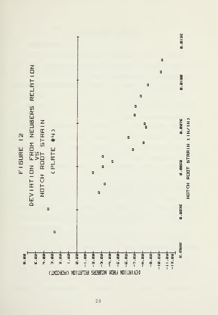
12. Deviation from Nueber's Relation (Plate #4) 28
13. Coordinate Transform (Finite Element) 32
14. Gauss Quadrature Points 32
15. Finite Element Model (POINTS) 33
16. Finite Element Model (POINTS) 35
17. Finite Element Model (Plate #1) 36
18. Finite Element Model (Plate #2) 37
19. Finite Element Model (Plate #3) 38
20. Finite Element Model (Plate #4) 39
21. Boundary Conditions and Loads on a 41
Finite Element Model
22. Finite Element Bilinear Assumption and 43
Stress-Strain Curve

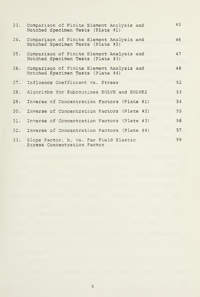
23. Comparison of Finite Element Analysis and 45
Notched Specimen Tests (Plate #1)
24. Comparison of Finite Element Analysis and 46Notched Specimen Tests (Plate #2)
25. Comparison of Finite Element Analysis and 47Notched Specimen Tests (Plate #3)
26. Comparison of Finite Element Analysis and 48Notched Specimen Tests (Plate #4)
27. Influence Coefficient vs. Stress 52
28. Algorithm for Subroutines SOLVE and S0LVE2 53
29. Inverse of Concentration Factors (Plate #1) 54
30. Inverse of Concentration Factors (Plate #2) 55
31. Inverse of Concentration Factors (Plate #3) 56
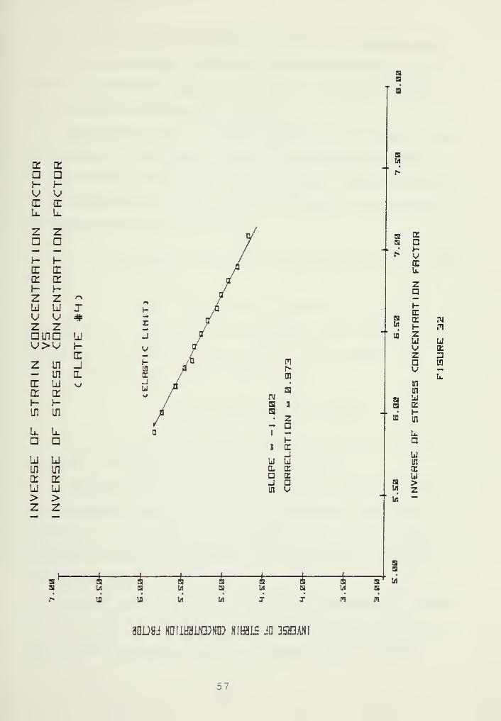
32. Inverse of Concentration Factors (Plate #4) 57
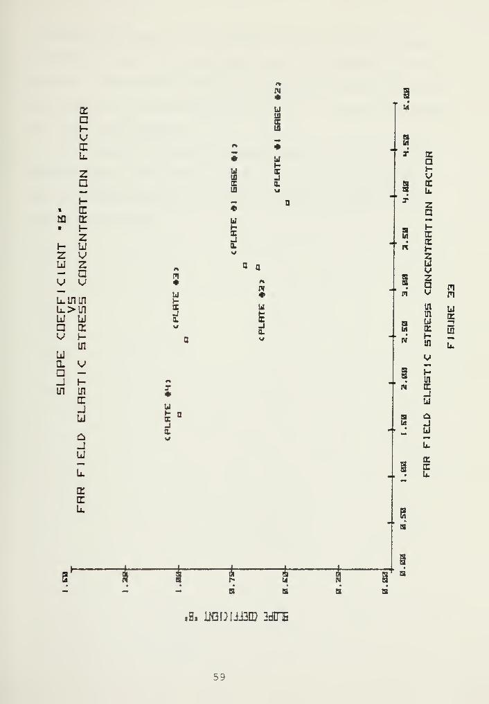
33. Slope Factor, b, vs. Far Field Elastic 59
Stress Concentration Factor


I. INTRODUCTION
A major goal of the Navy Aircraft Life Management Program
is to reliably and accurately predict the fatigue life of
aircraft structures. The method currently employed determines
structural life as a function of known structural and material
properties and of "g" loading, which is measured by acceler-
ometers in each aircraft. Since loads carried by the aircraft
structure for a given "g" load are also a function of vari-
ables such as airspeed, weight, altitude, angle of attack and
stores distribution, all of which are not measured, the
present method of estimating structural life', to be safe, per
force must be conservative; thus, aircraft can not be em-
ployed at their optimum cost effectiveness.
In order to obtain a more accurate means of determining
aircraft life, a fatigue monitoring system has been developed
[Ref. 1] . This system provides a direct airborne capability
for recording strains at critical locations in the structure
through the use of strain gages. Placement of strain gages
at a location of stress concentration is not practical for
long term applications, because fatigue of the strain gage
itself precludes the use cf this method. Therefore, the
strain gage must be located at a point on the structure near
the site of interest but undisturbed by the effects of stress
concentrations
.
An accurate relationship between applied strain, or far
field strain, and local stress behavior at a point of stress

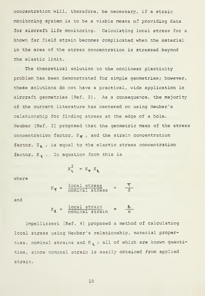
concentration will, therefore, be necessary, if a strain
monitoring system is to be a viable means of providing data
for aircraft life monitoring. Calculating local stress for a
known far field strain becomes complicated when the material
in the area of the stress concentration is stressed beyond
the elastic limit.
The theoretical solution to the nonlinear plasticity
problem has been demonstrated for simple geometries; however,
these solutions do not have a practical, wide application in
aircraft geometries [Ref. 2]. As a consequence, the majority
of the current literature has centered on using Neuber's
relationship for finding stress at the edge of a hole.
Neuber [Ref. 3] proposed that the geometric mean of the stress
concentration factor, K^. , and the strain concentration
factor, K e , is equal to the elastic stress concentration
factor, K, . In equation form this is
where
and
KK
" K<r
Kt
_ local stress" T nominal stress
local strain£ nominal strain
Impellizzeri [Ref. 4] proposed a method of calculating
local stress using Neuber's relationship, material proper-
ties, nominal strains and K^ ; all of which are known quanti-
ties, since nominal strain is easily obtained from applied
strain.
10

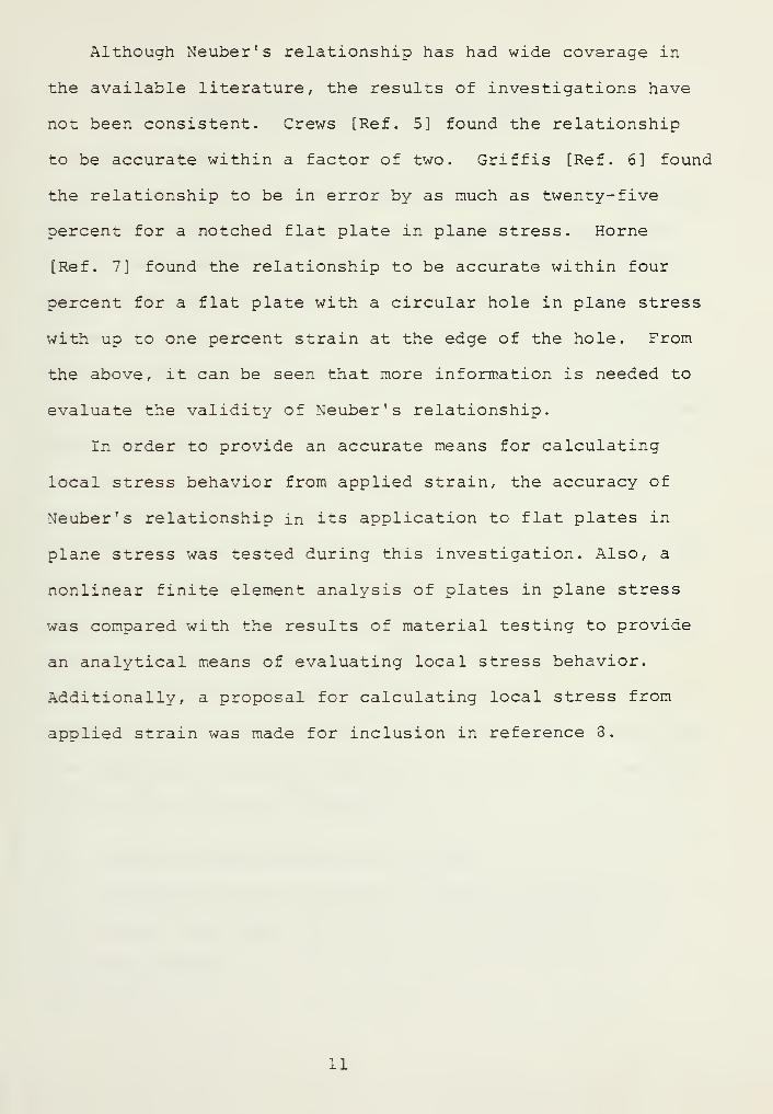
Although Neuber's relationship has had wide coverage in
the available literature, the results of investigations have
not been consistent. Crews [Ref. 5] found the relationship
to be accurate within a factor of two. Griffis [Ref. 6] found
the relationship to be in error by as much as twenty-five
percent for a notched flat plate in plane stress. Home
[Ref. 7] found the relationship to be accurate within four
percent for a flat plate with a circular hole in plane stress
with up to one percent strain at the edge of the hole. From
the above, it can be seen that more information is needed to
evaluate the validity of Neuber's relationship.
In order to provide an accurate means for calculating
local stress behavior from applied strain, the accuracy of
Neuber's relationship in its application to flat plates in
plane stress was tested during this investigation. Also, a
nonlinear finite element analysis of plates in plane stress
was compared with the results of material testing to provide
an analytical means of evaluating local stress behavior.
Additionally, a proposal for calculating local stress from
applied strain was made for inclusion in reference 3.
11


II. NOTCHED FLAT PLATE SPECIMEN TESTS
A. INTRODUCTION
In view of the apparent discrepancy regarding the validity
of Neuber's relation, tests were performed on notched flat
plate specimens in plane stress to observe Neuber's relation
and the relationship between far field strain and local stress
behavior at the notch root. To insure uniformity, all flat
plate specimens were manufactured from the same sheet of
0.090-inch thick 7075-T6 aluminum. In addition, all specimens
were oriented the same direction on the original sheet of
material and each plate was manufactured to fit a common
loading fixture used in the Riehle testing machine.
In all phases of specimen testing, strain gages were con-
nected to a Nheatstone bridge circuit, which has been cali-
brated for strain gage factor and temperature considerations.
The output of each Wheatstone bridge was measured by a
digital voltmeter and recorded on a stripchart recorder. An
event marker on the stripchart recorder was used to coordinate
the load with the strain gage trace. The load was recorded
by hand at convenient increments.
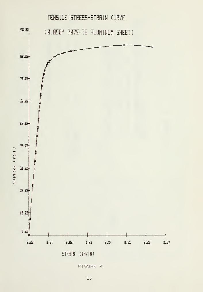
B. UNIAXIAL TENSILE STRESS-STRAIN TESTS
To determine the stress-strain characteristics of the
test plates, two flat plate uniaxial specimens were tested
in plane stress.
12


1
.
Description of Procedure
The first specimen was tested to accurately determine
the stress-strain relationship in the elastic range. Loads
were applied, held, and strains were read on the digital
voltmeter until creep in the specimen became significant.
The second specimen was used to investigate the stress-strain
relationship in the region of large strains. During this
test, the load was applied at a constant rate and strain data
were recorded simultaneously on the stripchart recorder.
Figure 1 shows the instrumentation used to record strain data.
2
.
Test Results
For both specimens, stress was calculated from load
data for a corresponding level of recorded strain. The results
of the tests were combined to produce the stress-strain re-
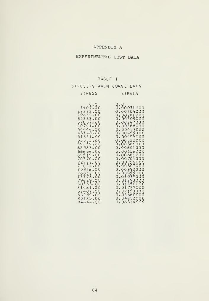
lationship for the test specimen material. Table 1 of
Appendix A and Figure 2 contain the results of the uniaxial
tensile stress-strain test.
From test results, the modulus of elasticity for the
test material was determined to be 10575 ksi, and the yield
stress was determined to be 7 5 ksi.
C. NOTCHED PLATS SPECIMEN TESTS
Notched flat plate specimens were tested in plane stress
to investigate Neuber's relation and the relationship between
far field strain and stress at the notch root. Four specimens
with different notch geometries were utilized in the test.
Figure 3 describes the four plate geometries and strain gage
placement.
13


14

TENSILE 5TRE55-5TRR1N CURVE
MM(0.030' 7075-TE RLUMINUM 5HEET)
.22+
7H.ffl-
S.22-
3JI-
2.22 H.HI a.22 z.ai a.HM Z.2I 2.25 0.H7
STRAIN (IN/IN)
riSURET 2
15


Ld
X
Hninzzu
L.Z
ZLdDEL-Ulh-
CLI--inCLUi
in
u
a:uj mtil
zZzId Nz
UIEL
in -
«
a
am
m
a
s
J a
1
a:
r i-a:
1§5
ans XXrv y-— Hh
1 ! Zam yiXtfl ui ^a13 N XVU1 — k ••u.-N n zIS a »m «« -s
.. mm •* y *-!**
U 1 Ui 13 XHxx N Z U •
>Li — X Sl- in X J
in &WH y UI yyIflZ 12 in UJHHxy X X xxaIEZ m IS ifl^ny ax
ZX z z Z.J-Z3 — — - XXlfl X X xyvXX X X XU31-1— UJ 1- H hlDini in in UllOZ
in
yHaz
n
yx
13
? r
16

In addition to the strain gages shown in Figure 3, an
extensometer was placed in the region of far field strain.
Strain data from the extensometer were recorded by the Riehle
testing machine as the machine recorder produced a graph of
applied load versus extensometer strain.
1. Test Procedure
The instrumented specimens were loaded by the Riehle
testing machine with a constantly increasing tensile load.
Figure 4 shows test specimen number four mounted in the
machine. As the load was applied, strain data were recorded
in a manner similar to that described for the uniaxial tensile
stress-strain tests.
The tests were terminated for plate number one when
the gage limit of three percent was exceeded; for plates two
and three after both gages had failed; and for plate four
when the load limit of the loading fixture holding the speci-
men was reached.
2
.
Test Results
To analyze stress and strain behavior at the notch
root, the data recorded at the notch roots were averaged.
To determine stress from strain data, the data obtained in
the uniaxial tensile specimen tests were used in a regression
scheme that calculated a stress for any given strain. Far
field stresses and strains and nominal stresses and strains
were calculated from a knowledge of the load, plate geometry
and modulus of elasticity of the test material.
Tabular data from the notched specimen tests are
presented in Tables 2 to 27 of Appendix A. In the tables of
17

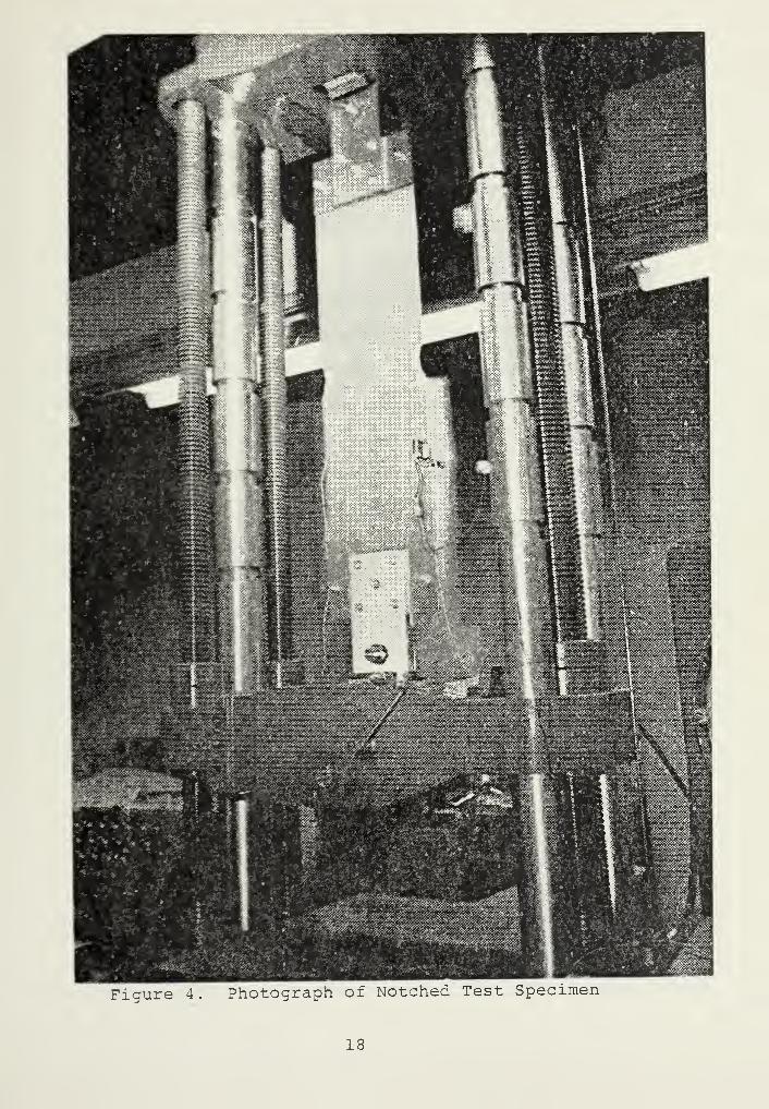
Figure 4. Photograph of Notched Test Specimen
18


Appendix A, stresses 1 and 2 and strains 1 and 2 refer to
stresses and strains at the notch roots. Stress and strain
number 3 refer to extensometer data. It can be seen that
strains 1 and 2 are in disagreement by 10 percent for plate
number 1 (Table 2) . This is attributed to strain gage lo-
cations not being identical on both notches and the rapidly
changing stress gradients in the notch root area of plate
number 1. As the notches became less severe, the differences
between notch root strain gage readings became less. The
notch root strains recorded for plate number four are almost
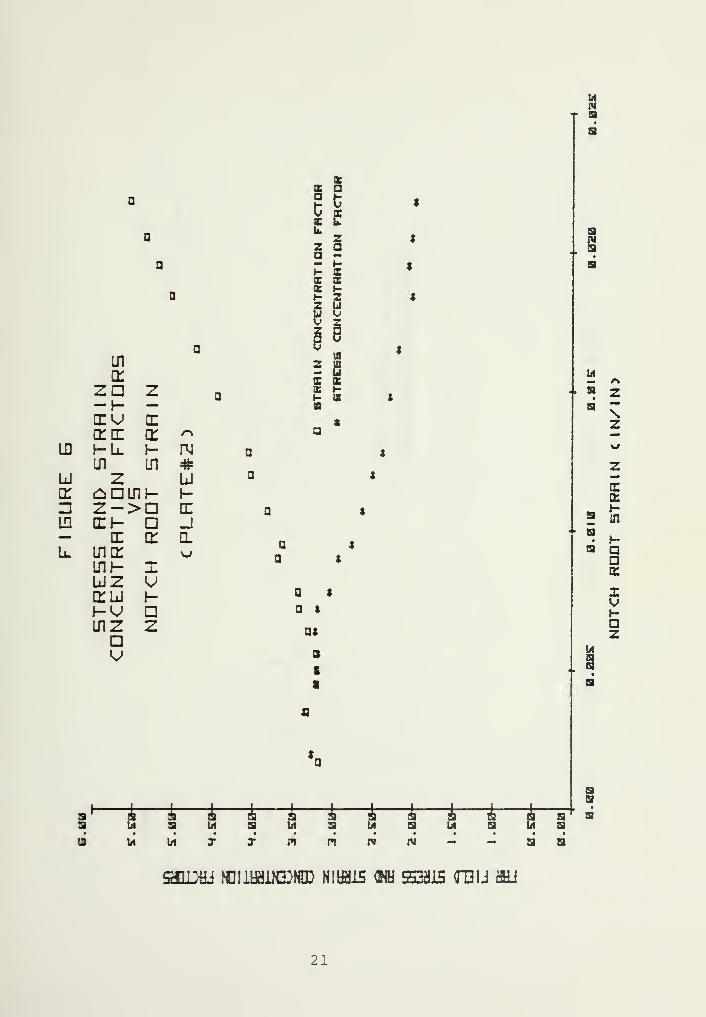
identical. Figures 5-8 contain a graphical presentation of
far field stress and strain concentration factors versus notch
root strain for plates 1 thru 4, respectively. Far field
stress concentration factors have been defined as the ratio
of notch root stress to far field stress. The far field
strain concentration factor has been defined similarly.
The experimentally determined elastic far field stress
concentration factors for the notched test specimens were as
follows
:
Notched Plate Number Elastic Far Field StressConcentration Factor
1 3.60
2 3.23
3 2.45
4 1.65
The far field elastic stress concentration factor can be re-
lated to the traditional elastic stress concentration factor
by the ratio of the far field area to the nominal area, which
19


s
in
kzp-Haru
Lrl EH zHk _ /%
U in cn-B z a:#n aa h-
ifl z—tninu— CTH> 1-
u. C f-CEina -J
mi— DO.wz o:wcru}-^ iU1Z ^
h-U a
z
I
1z8
8 z
I Ii-
ga
aa
no
i a
taai
z
zs i
s1—I—I—I—S—t—I—3—
I
S50J raumMMD ffi&is <w ssaiis rau an

in
o:
zn Z o-h- —\LK> CE
ctce cr r\
10 Kit h- H4 aU1 Ul #
LJ z LJ a
K AdLTlf- h-
n z->n EC
in El- n -J— IE ET CL
u.
5TRE55
CDNCENTR
X
z
\j
k a
I 6
EEz
z aa -- »-H SX XK Ht- Z
111
^ aI (XX Ht- a
UNB
SIV3
aa
a *
a *
a*
B
i
sBU
4—t—4—*-1 B Ik S
T
i—
i—i
—
t—
i—t-
s Q b Q s Q
u— r,
z
Z
aui
b aaa:
iI-az
VI
„ I
sB
PI W
s s5
SEDHJ HDIiffliNDfCD NIfcfiLLS ttU 33815 0T3U HHJ
21


a 1 a a
a $e £
a t z za a
a 1TRflT
1
TRflT
1
in a t
q: a t s sZD z V
cr
a
na
t
1
Z Z8 8
r*
etd: q:
3 °o1
1
Z Ifl
Ifl in 1- 1-
u z£ 1
ii a
a: ^aini- n *
D z->a E U 9
l£3 CEH a -J at— tr cr Q.b_ in a:
ini- Xv-f
LJZ V i
cru 1-
h^ ainz zaV
a—
»
aa
8aa
aaaa
z
z
a zs* E
o:t-ui
a **a
« 5az
unaa
10
i 4 i 1 1ut a li a y
* taa
sa
aa
n w w - - a
9DDHJ N01JMLNTNID N1UB1S OXH 23815 TDIJ fflJ
22


14
t «
a4, a
aa
in a *
o: 8 SZD z a s
-h- — a j
CU IE r\
trir cr T a t
TIDN
1
min
# a i
u z Li 01
IT aauu- h- aiH ZZ U
z aD z->a EE
MP
aII] cri- a -J— rr cr H 8 a v
h- ijiq: \j 1 IB3 tfl
\su- i 84* Ui- u
liJZ v i tcru i- in
|-<v> a a ginz z aav
3
i a
a* t 'A
Ur- <»a Z
a Sz
8
cJ-Ul
u. I-a a
aa:
Ii-
zuNaa
aa
SaiJDHJ NDIUfiLLKDNlD MW1S ffU EB15 0T31J fflJ
23

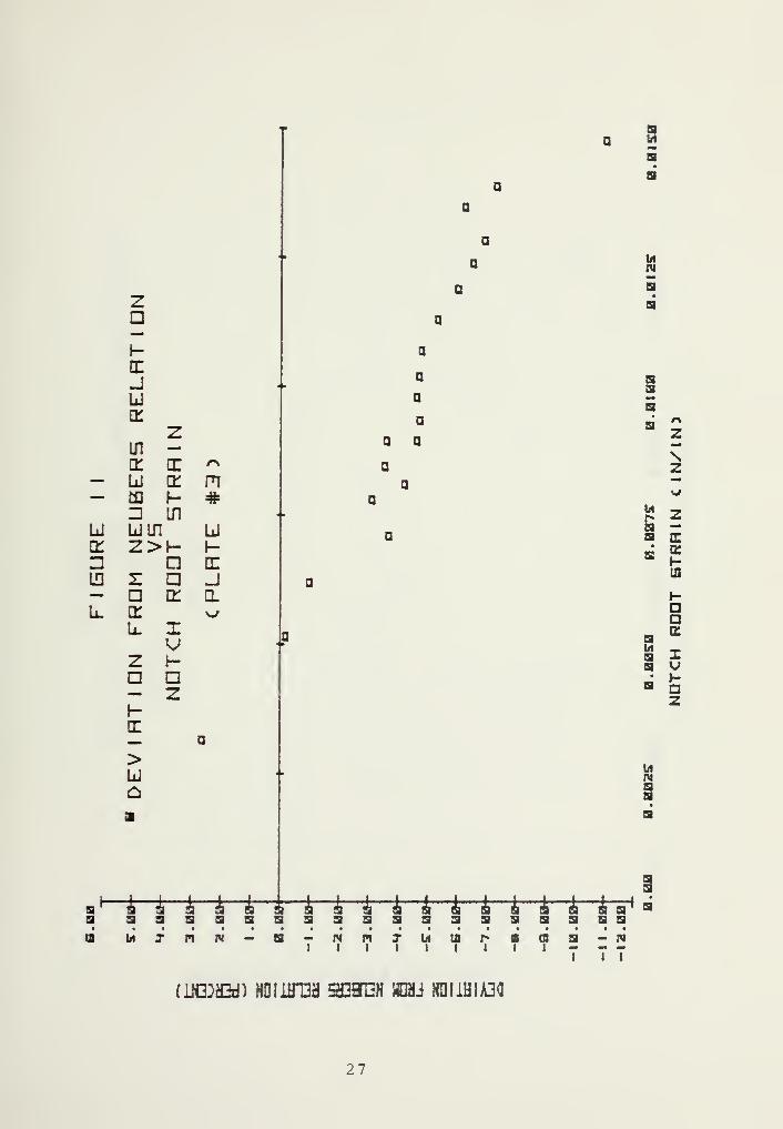
is the net cross-sectional area of the plate taken at the
notch.
Figures 9-12 show the deviation of the test data
from Neuber's relation. The data plotted for plate number
two in Figure 10 have a discontinuity in the region of 0.6
to 0.8 percent strain. This is attributed to poor data
obtained from strain gage number two prior to its failure.
It can be seen that once the notch root strains reach the
region of plasticity, Neuber's relation is in error to a
significant degree. It can also be seen that the error in-
creases as the level of notch root strain increases.
24

1-
E_I
utr
Zin —k EE
y ET01 m f-^
d Ul-u UJ #CK ZlfiHD >nu10 z i-— n o:a:L. n -j
u. ID.
z *-
a P— zi-CE
>U&
B
*—i—4-
B SB
B
sz
S ECK
B Hifl
»-
aaEK
x
nz
BS
BIII
4—i—i
—
t—t
i
BBT
sbi
7B Irt
I I
BBBni
( JJCDtDd ) NOllirH! 2D3H3H HOU N0IUHA34
25


MNa
za
i-
ee
juq: z
in EE r%
IS ET IT rvi*^— Ld
m#
Id Zl Ldtr yinn h-Z3 z>a X a113 a _J— z cr Q.U. a v-/
a
CE XL.
i-
Z aa z
i-
CE
>u&
ss
t-tr-t-t-tr-t-t
« Z
z
IKJ-
2m
B I-
Sa:
i«*>
z
t>i
sa
Hr* u ui
BT
t-t-t-t-t-t-f-u 1
aa
a s
n n - s - w PIt i 1
\a a > n
ClNTffid) NDiiHT3fl SGIQN HDHJ NQI1HIA24
26
z
h-
cc
-1
Li
cr
zin —tr cc /^
—LaJ a: n— m i- #n LH
Ld um Ld
Z Z>l- i-n n a:LD z a _j— a n: a.
U. or v-f
k. i
z 1-
a n— zi-
EE— a
>UJ
A
aa
aa
a
a
a
a
a a
a
aa
1aa'
t-t-ir-k-k
z
z
a c
tfl
Haa
a *
a K>
a oz
1/1
I
aa
a a a a a a a J, a a aa a
m n - a - w pii i i i i
a a - w
7 T T
^JJGJiGd) HDliHT3a SQ9I2N HOHJ NnilH!A3a
27

unaa
f-
OC-J
LI
ET
in
cr
Li
m zD —U IT /-v
N z cr T— i- #z in
Id a LJ
cr crmi- 1-
D u.>a ECID a -J— z a: a.
L. a yj— Xi- <J
cc f-— n> zua
a
aBaa
a
a
aa
14 ~
sa z
ai-
s *
§ {=oa q
tr
i
z
a9 ssaaaaasasaasaaaa
aaa
i I a
in n - a - ra mt i
XI
\a aj l
UKDffid) HDIlHTai 2£HBN HQU NDIiH!A3<I
m a - nT 7 T
23


III. FINITE ELEMENT ANALYSIS
A. INTRODUCTION
The finite element method has proven to be a powerful
tool for analysis of complex problems in structural engineering
A dominant reason for its quick acceptance and extensive ap-
plication in engineering practice is due to its complete
generality
.
For the reason of generality, this investigation examined
the feasibility of forming an analytical method of observing
local stress behavior in the area of stress concentrations
for flat plates in plane stress. If the results of a finite
element analysis compared favorably with actual test data,
it could be postulated that models of other stress concen-
tration factors and material properties would be equally
valid.
1. Survey of Available Finite Element Analysis Programs
Finite element programs available at the Naval Post-
graduate School were surveyed for the best available program
to use in a nonlinear finite element analysis of flat plates
in plane stress.
The scope of nonlinear programs available was quite
narrow. Program EPLAS [Ref . 6] has been translated to FORTRAN
IV and made operational. Programs NONSAP [Ref. 9] and ADINA
[Ref. 10] were also operational and available. Program EPLAS
used a scheme of constant strain triangles in an analysis of
plates in plane stress. Because the intricacy of the small
29

triangles required to define the area of stress concentration
did not lead to easily redefining the model, program EPLAS
was not considered appropriate for this investigation. Pro-
gram NONSAP contained a library of element models as well as
material models, and it was considered appropriate for this
investigation. However, the most flexible and convenient
to use of the three programs surveyed was program ADINA
(Automatic Dynamic Incremental Nonlinear Analysis)
.
Program ADINA is a general purpose linear and non-
linear static and dynamic finite element program. Structural
matrices are stored in compacted form and element information
is stored by blocks in low speed storage. The program is an
out-of-core solver; i.e., the equilibrium equations are
processed in blocks, and very large finite element systems
can be considered. There is practically no high speed storage
limit on the number of finite elements used.
For nonlinear response, an incremental solution of
the equilibrium equations is used. The linear effective
stiffness matrix, the linear stiffness matrix and the load
vectors are assembled in low speed storage. During a step-
by-step solution, the linear effective stiffness matrix is
updated for the nonlinearities in the system. The incremental
solution scheme corresponds to a modified Newton iteration.
To control accuracy, the number of steps between equilibrium
iterations and between reforming a new effective stiffness
matrix can be controlled by the user.
30

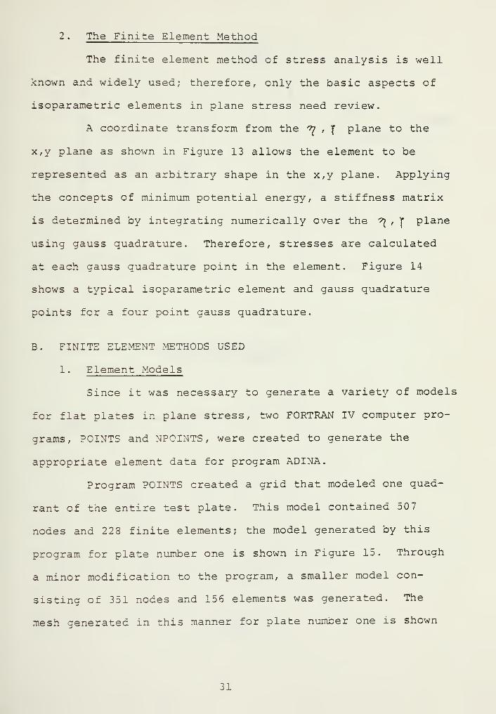
2 . The Finite Element Method
The finite element method of stress analysis is well
known and widely used; therefore, only the basic aspects of
isoparametric elements in plane stress need review.
A coordinate transform from the "7?, f plane to the
x,y plane as shown in Figure 13 allows the element to be
represented as an arbitrary shape in the x,y plane. Applying
the concepts of minimum potential energy, a stiffness matrix
is determined by integrating numerically over the ^ , t plane
using gauss quadrature. Therefore, stresses are calculated
at each gauss quadrature point in the element. Figure 14
shows a typical isoparametric element and gauss quadrature
points fcr a four point gauss quadrature.
B. FINITE ELEMENT METHODS USED
1 . Element Models
Since it was necessary to generate a variety of models
for flat plates in plane stress, two FORTRAN IV computer pro-
grams, POINTS and NPOINTS , were created to generate the
appropriate element data for program ADINA.
Program POINTS created a grid that modeled one quad-
rant of the entire test plate. This model contained 50 7
nodes and 228 finite elements; the model generated by this
program for plate number one is shown in Figure 15. Through
a minor modification to the program, a smaller model con-
sisting of 351 nodes and 156 elements was generated. The
mesh Generated in this manner for plate number one is shown
31

figure: i]
n -x a
f aoaeiRNT
mU5S SURDRflTURE PQ1NT5
CM POINT 5RU55 QDHDRflTURe)
F1EURE IH
32


&Idh-CECELdZu inL£3 h-
z_I —LJ p& CL
ar Z
IT
H q:z LDLd nX aLd CL
_JId >
toIdh-
I I / / /;;
i TT /j"
\ i a i / // rrj
I II J/J- sj'
sA
J*
L/1
Idcr
m
33


in Figure 16. In view of the theories of St Venant, the
smaller model was considered adequate for use in this analysis.
Program NPOINTS was a smaller version of program
POINTS. It created a grid that was the same size as the
smaller model generated by POINTS. Although equal in physical
size, the model generated by NPOINTS contained 189 nodes and
78 elements. A model generated by NPOINTS for plate number
1 is shown in Figure 17.
Both mesh generation programs were general in nature.
By simply redefining the vector of variables which described
the notch at the edge of the plate, a new mesh could be
generated. Both mesh schemes were tested for accuracy and
efficiency in program ADINA.
For the plate model tested, the two elastic stress
concentration factors calculated using the two mesh schemes
were essentially equal. The mesh generated by POINTS re-
quired 26.5 minutes of computer time for 20 load applications,
while the mesh generated by NPOINTS required 23 minutes of
computer time for 20 load applications. On the basis of
relative efficiency, the mesh generated by NPOINTS was
selected as the model to use for the finite element analysis
portion of this investigation. Models generated by NPOINTS
for notched specimens 2, 3, and 4 are shown in Figures 18-20
respectively. All plates were modeled so that Gauss quadrature
point number 3 in element number 1 coincided with the center
of the strain gage on the actual test specimen.
34


FINITE ELEMENT MDDEL GENERATED
BY PROGRAM PQ1NT5
FIGURE IG
35

FINITE ELEMENT MODEL FDR PLATE #
EENERRTED BY PRD5RRM NPD1NT5
FIGURE 17
36

FINITE ELEMENT MDDEL FDR PLHTE *2
EENERRTED BY PRQERRM NPQINT5
15 12
3
JO
3•1
5 5
FIEURE IB
37


FINITE ELEMENT MODEL FDR PLRTE *3
EENERRTED BY PRDERHM NPDINT5
F1EURE 13
38

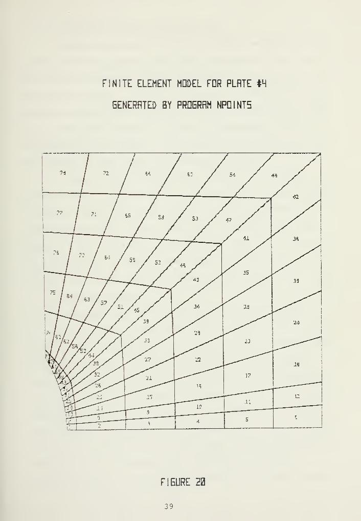
FINITE ELEMENT MDDEL FDR PLRTE *H
GENERATED BY PRDGRRM NPDINT5
F I SURE 20
39

2. Symmetry and Load Considerations
Meshes generated by program NPOINTS, as shown in the
above mentioned figures, model only one quarter of the plate.
The plates are symmetrical and two planes of symmetry cut
through the plates. Therefore, as shown in Figure 21, by
imposing the boundary conditions of zero displacement in the
y-direction for boundary 1, and zero displacement in the
z-direction for boundary 2, it is necessary to model only
one quarter of the plate for a complete analysis.
Loads can be applied to the model only at nodal
points; Figure 21 shows the formulation of the applied loads.
A uniform stress is assumed across the boundary where the
loads are applied. A load that would produce one half the
stress in the element is applied at one node and an equal
load is applied to the opposite node. If two elements share
a common node, the loads are summed at that node.
3
.
Material Model
Program ADINA provided for the use of a bilinear
stress-strain relationship when defining the material proper-
ties of the two-dimensional continuum elements. The material
model used was the elastic-plastic (von Mises isotropic
hardening) model. This model is defined by Young's modulus,
Poisson's ratio, yield stress in simple tension and a strain
hardening modulus. To model the actual properties of the
test material, the modulus of elasticity as determined in
the uniaxial tensile stress-strain test was used as Young's
modulus and 0.3, a standard for aluminum, was used as
Poisson's ratio. A linear least squares fit of the uniaxial
40


SDUNDRY CDNDITIDN5 HND LDRD5
DN fl FINITE ELEMENT MDDEL
FU1C OF 5YWCW *2
FIGURE 2
41


tensile stress-strain data between 1.0 percent and 2.1 per-
cent strain was used to calculate a hardening modulus of
399.606 ksi. The intersection of the modulus of elasticity
and the line defining the hardening modulus was taken to be
the yield stress of 77.173 ksi for the model. Figure 22
shows the bilinear stress-strain assumption compared with
the uniaxial tensile test data.
4 . Analysis Procedures
A four point Gauss quadrature, which is the allowable
maximum, was specified in the program input parameters to
obtain results as close to the notch root boundary as
possible. Because of this requirement, out of core storage
requests in the standard ADINA JCL cards of reference 10 had
to be modified to accommodate the size of the system being
analyzed. The loads applied to the nodes shown in Figure 21
were applied in thirty increments. The first four loads
were scaled to create a stress at the notch root equal to
the yield stress. The remaining twenty-six increments were
evenly spaced between load number four and the highest load
recorded during the corresponding notched flat plate specimen
test.
C. RESULTS OF FINITE ELEMENT ANALYSIS
Tabular results of the finite element analysis using
program ADINA are in Appendix B. The comparison of far field
stress concentration factors from the finite element analysis
and the notched test specimens were as follows:
42


a. 22
BB.ffl-
FIEURE 22
FINITE ELEMENT BILINEAR R55UMPTIDN
BND
5TRE55-5TRRIN OJRVE
.11 B.E I.C B.3H B.K 2.BS H.ffJ
STRAIN (IN/IN)
43

Far Field Elastic
Stress Concentration Factors
Plate Finite Element Specimen Test Variance
1 3.92 3.60 8.9%
2 3.33 3.23 3.2%
3 2.51 2.45 2.4%
4 1.63 1.65 1.2%
The results of the finite element analysis compared favorably
with the results obtained from the notched specimen tests
for plates 2, 3 and 4. In addition, if the far field elastic
stress concentration factor for notched specimen number one
was calculated using gage number 2 only, the variance would
be 3.4 percent, comparable to the other plates modeled.
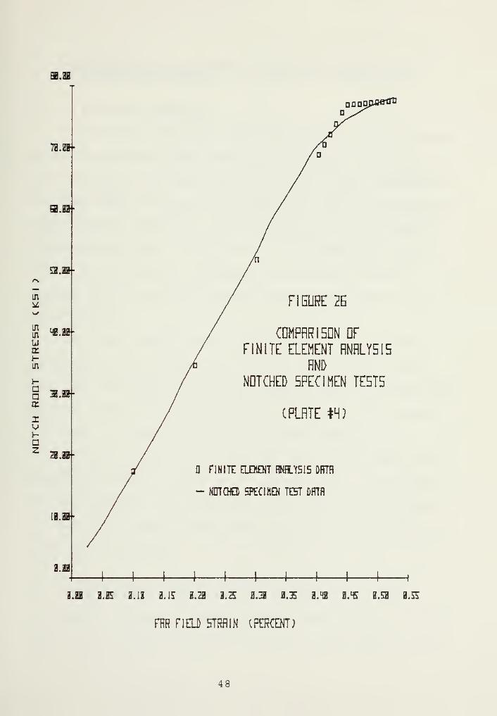
Figures 23-26 compare notch root stress versus far field
strain for the tensile test specimens and the finite element
model. The correlation between finite element analysis and
tensile test specimen data also compares favorably in
Figures 23-26. The trend of the notch root stress to increase
more rapidly after reaching the 30 ksi range is attributed
to Gauss quadrature points in element number two becoming
plastic and dramatically changing its ability to carry a
load. The effect is especially noticeable because of the
difference in size of the elements.
44


52.23
B0.HB-
7H.2B-
m.m
in
w £2. ga-in
uEfr-
ill
act
i
z
23.HB-
ib.d-
F1EURE 23
CDMPRR 1 5DN DF
FINITE ELEMENT RNRLY515
FIND
NOTCHED 5PEC1MEN TE5T5
CPLRTE #1)
O FINITE OQOT BNH.Y5I5 DATA
- NDTQO SPeClMEN TOT DHTH
2. 23
-f- + +2.221 0.2fl2 2.M3
FAR FIELD STRAIN (IN/IN)
0.02H
45

a.aa
SB.HB-
7B.flB»
ffl.flfr-
in
-3 a.©uKUl
a VJM-aB
§ 3.Z2-
aji-
n.fflf
a.ffl
a n
FIEURE 2H
CDMPHR I 5DN DF
FINITE ELEMENT RNRLY515
AND
NOTCHED 5PEC1MEN TE5T
(PLRTE #2)
FINITE ELEMENT RNHLY5I5 DflTfl
- NOTCHED SPECIMEN TEST OBTfl
l.Zl 1.E2 2.22 2.3 3.22
FBR F1EU STRAIN (PERCENT)
3.33 H. H.sa
46

.fflf
7H.HB-
a.zaf
a o a do,
in
min
ucr
I-
m
aaa:
i
Z
HB.ffi-
38.2a-
a.za-
FIGURE 2E
CDMPRR 1 5DN DF
FINITE ELEMENT HNHLY5I5
RND
NDTCHED 5PEC I MEN TE5T5
(PLATE *3)
O FINITE ELEMENT RNfU515 DBTfl
- NOTCHED S^CIMEN TE5T Dffffl
IB.ffi-
1 1 1 1 1 1 1 1 1
IM l.E g.lfl i.JS 3.22 2.25 B.3H 0.35 H.Hfl fl.HS
FRR FIELD STRAIN (PERCENT)
47

nonoj
7B.H&-
ffl.tt-
g.ffl-
m
UKHin
t-
q 2.H81 "
BI
I-
Dz
a.ffl-
1B.HB--
FIGURE 2G
CDMPHR 1 5DN Df
FINITE ELEMENT RNHLY5I5
RND
NDTCHED 5PEC1MEN TE5T5
CPLRTE #H)
FINITE ELEMENT H*fflLY515 DHTH
- NDTOO 5PEC1HEN TEST DATA
I 1
a.£ a.ia a. is a. 23 2.2? a.a 2.3 b.mh a.« a.sa a.ss
FflR FIELD STRAIN (FEEOTH
48


IV. INVESTIGATION OF METHODS TO RELATE FAR FIELD STRAINTO NOTCH ROOT STRESS
A. A HEURISTIC ANALYSIS
A heuristic analysis of far field strain and notch root
stress was pursued after observing in Figures 23-26 that the
plot of notch root stress versus far field strain maintained
the same shape, although in a compressed form, as the original
stress-strain relationship obtained in the uniaxial tensile
stress-strain tests. Therefore, a local stress far field
strain relationship was developed by dividing the local
strains by the far field stress concentration factor, for a
given stress.
For each notched test specimen, the new stress-strain
relationship was developed and the far field strains from
each test were used to verify the relationship by calculating
stresses using the new stress-strain relation. The results
are found in Tables 5, 12, 18, and 24 of Appendix A.
As can be seen from the tabular data, the stresses com-
puted in this manner vary up to 4 percent from the stresses
actually recorded during the testing of the notched specimen.
It can also be observed that the error increases as the notch
root strain increases.
B. A FAR FIELD STRESS AND STRAIN CONCENTRATION FACTORPOWER RELATION CURVE FIT
Another attempt to relate the far field strain and notch
root stress involved finding a relation between the far field
49


stress and strain concentration factors. The method used
to relate the two concentration factors was a power curve
fit. In equation form it was assumed that
KT
= (a) (K £ )
or
(T/S) = (a) (£/fi ^
Assuming that for every stress, there exists an in-
fluence coefficient, E' , such that stress is the product of
E' and strain, the above equation can be written
T = SaCT/E'e)^
solving for the notch root stress,
T = e(Ea/(E') V""^
Since this relation must also hold in the elastic limit
(E'=E) , the coefficient, a, must be given by
t-V \-v»
a = (T /Ee) = (Kt
(ff)
)
Therefore, substituting into the above,
T = e(K t (ff) ) (E/(E') ^)
V_Va
Two unknowns still remain in the above equation, the
notch root stress and the influence coefficient, E'. There-
fore, an iteration scheme using the relationship between
stress and E' is necessary to calculate the notch root stress
using this method.
50


To evaluate the relation of stress and E*, the stresses
of the stress-strain relationship (Figure 2 and Table 1) were
divided by their corresponding strains to calculate an E 1
for that stress. The results are found in Table 6 of Appen-
dix A and a plot of E' versus stress is found in Figure 27.
A power curve fit method was used to calculate the power
factor, b, from the data of far field stress and strain con-
centration factors.
Subroutine SOLVE of a data reduction program calculated
the notch rcot stresses given an input of the far field
strains. Figure 28 is a flowchart describing how subroutine
SOLVE functioned.
The tabular results of the notch root stresses calcu-
lated by SOLVE are presented in Tables 7, 13, 19, and 25.
Table 26 provides the data calculated to be the curve fit
exponent. The tabular results show differences of up to
fifteen percent between calculated stresses and actual stresses
found in the notched specimen tests. It should be noted,
however, that only one refinement was made in iterating to
find the E' that related to the calculated stress.
C. RELATING THE INVERSE OF THE FAR FIELD STRESS AND STRAINCONCENTRATION FACTORS IN A LEAST SQUARES LINEAR CURVEFIT
A third method of relating the far field strain to the
notch root stress was to use the observation that the inverse
of the far field strain concentration factor plotted against
the inverse of the far field stress concentration factor was
essentially linear. Figures 29-32 describe this relation
51


aaam
aaaa
aaa
in
in
id
q:
i-
in
m>
Zid
L.
Id
aaa
aaa
aa
a*x
aaan
in
in
in
uET
in
m
in
U
zId
aaa*N
zaa
35
N
aa
s
B
aeg
m
a a«
N
aa
aa
fJIX ISd) DDmiflD} BOTUN!
52


fLGDRiTui m smsmm stlvx i mmINPUT m FIELD 5TRRIN
(DO I* l/NPHFI
J>
ataurre notch hot stbesffi R FUNCTION DF
INRTT 5TRES SB EKI)
YE5
TD FIND EPCHI INTHH.
CUNTINUE
HRITE
'NO RDOT FIHtt'
<g>
E' -(Ftf) *E!')/2
OLOJLRTE HDTCH RDQT 5TRE5
fG R FUNCTIIW DF
INRTT 5THE55 RND V
HRITEREHIT5
FJEUE2R
53


sto
cr cr
a ah »-
V uDC CE
U. L.
Z Za D
H HEE CE
IX cr
H HZ Zu _K> VZ zamau>uZ Ul— in
CE ucr cr
i- j-
in w
L La D
u UJ
m in
cr cr
Ul u> >z z
Ld
h-
CE
-J
CL
mUl
01
m S01p» 1
m• ZH a1
*•
H1 lE
-1U Ua. cra a:-i a01 w
sT
-4-
sN
4-
5
s crX Ds
CL
Za»-
Bcr 01
»- NS z
y y
za
it
IS
w; b.
in
in
s yw
B
B
in
Layin
y>z
B -
Ss
HODHJ NlJliHHiN3)NQ) HIW1S £ 3SQANI
54


as«
10
EE X
1- i-K> uEE CE
U L.
z ZDH HEE CE
a ce
H HZ Z /*\
Ul UJ w<v» V #z zninn LJ
u>^ HEE
z in J— in EL
EE y wEE EE
H Hin in
k u.c D
Li Ixi
in in
ET EE
u U> >z z
Id
Ul
ID
m
smn i
u• zB1
aj-
t5
a3
y
i
6
SBS
i
8pi
aUEU.
za
Ha:CE
ZUza
ui
in
yVLH10
Ll
ayin
a:u>z
i
HPI
yxa10
tain
*§T N
BOU HDIlffliHOTD MIB15 JD 3^3AH!
55


sm
cr ka ai- j-
v v^
cr EE
L. L.
z z £a a J
i- h-^
CE CE »-
cr cr in
cri- l-
z z /"\ uu u n v
v v #z zainn uV>«v>
CE
z in J- ui a.
CE u v^
cr cr
i- i-
m in
L_ u.
a a
u uin in
cr cr
UJ u> >z z
CI
in
ms 5PIIs- 101
• ZB a1
—
•
H-1 C
-'
u UJ
a. aa cr-i ain v*»
»
sa
X Xa
Hi
n-t
s B
aa
5 cr
aHCk
lit
X zs a
CaHzs u _
X v ns z
a uw cr
3in in
Ul -»
w u L.
rc cri-
5 ui
u.ay
B inn cr
s >Z
inP4
B
HDDBJ NDJimOTD NIBSI5 JD 3SH3AN!
56

ss
cr cr
aK- hU ucr cr
L. Lu
Z ZD a
H i-cr CE
E cr
H HZ Z •>
Ld u TV ^ +Z Zauia LU<^>^ 1-
CE
Z in _l— Ul CL
cr u VJ
cr cr
f- i-
in Ul
b. Lu
P
lil bl
U1 in
cr cr
Ld UJ
> >z z
s
ui
nr-
m
3niIS S
a• z— D
i—
*
1-
i EE
-J'J Li
c aa a:
jUl w
su
a cc
s a
cL
Z
BUl
ui
k 1-
5ui ui
s 5 a sts ui
Xs
XUl
i-
lT
ZUi
za
in
in
a k» in
a
uin
z>z
sUl
ui
ssui
n
u
Ifl
3DUBJ N0I1HHIXM) KlffilS JO 35H3ANI
57

as well as the computed slopes and correlation coefficients
using a least squares polynomial regression of degree one.
Figure 33 shows the relation of slope, b, to the far field
elastic stress concentration factor.
The elastic limit in Figures 29-32 is at the point where
the inverse of the strain concentration factor equals the
inverse of the stress concentration factor. All data in the
elastic range will, theoretically, be plotted at this point.
Therefore, it can be shown that
(1/K t (ff)) = (1/K t (ff)) -b [(1/KT (ff))-(l/Kt (ff))]
or
e/€. = (1/K*(ff)) -b l(S/T )-(l/K t (ff))]
Assuming as in the power curve fit method that stress is the
product of an influence coefficient, E 1
, and strain, then
solving for stress, it can be shown that
T = EeK ^ (ff)£(b+(E'/E) )/(b+l)]
It is obvious that if E is substituted for E 1 in the above
equation, the elastic condition is satisfied.
Subroutine S0LVE2 of a data reduction program used the
same influence coefficient concept as described previously
in Table 6 of Appendix A and Figure 27. The scheme for cal-
culating the notch root stress for a given input strain was
the same as described in Figure 28.
Tabular results using this method are presented in Tables
3, 14, 20 and 26. Examination of the tabular data shows that
the stresses calculated using the linear curve fit method
58
L.
Za
» CE
• H-zLd
za
zu
U.U1U1ti->lfl
cr
fr-
ill
n
bl
Q. Va -
tn in
a:
ui
y
a:
cu
2
N•LILfl
3_
#» +VM
• UM &U Jtc a.u v»
M*ufcJa.w
*\ a an
1Mu«-
s UJa. §
_ *
X*
uEQ.
i—
r
s
Xa
B li.
X za
3 a:• a:n
Zu
§•
m
z3tn uin X
5LJ
a:3in
* »-N
in iZ
§« in
W a:
a au -j•
IT
§ EC• b.
i fr
g
.e. 1*01)11430) 3dtTE
59


differed by as much as ten percent from the actual stresses
recorded in the notched specimen tests. It should be noted,
however, that only one iteration was used in determining the
coefficient, E', to use when calculating the notch root stress
for a far field strain.
The relation between the slope factor and far field
elastic stress concentration factor as shown in Figure 33
was not readily apparent and not considered further during
this investigation.
60


V. CONCLUSIONS AND RECOMMENDATIONS
A. NEUBER'S RELATION
The results of the notched specimen tests indicate that
Neuber's relation is in error by as much as ten percent when
strains are less than one percent. As the strains at the
notch root became more significant, Neuber's relation became
less accurate with fifteen percent error at two percent
strain and twenty percent at three percent strain. It can
be concluded that methods of calculating local stress using
Nueber's relation would be susceptible to the same inaccura-
cies .
3. FINITE ELEMENT ANALYSIS
The results of the finite element analysis of notched
flat plates in plane stress using program ADINA correlated
well with the results obtained in the notched specimen tests,
The only limitation on program ADINA appears to be its model-
ing the element material in the plastic range in a bilinear
stress-strain relationship. It is therefore recommended
that element model number fifteen of program ADINA be de-
veloped in order to define the material more closely through-
out the range of strains to be encountered in the area of
the notch root.
C. DETERMINATION OF NOTCH ROOT STRESS FROM FAR FIELD STRAIN
The Heuristic analysis investigated in Section IV is
simple to use and economical with respect to computer time
61


used to perform the calculations. The heuristic method is
much more accurate in the nonlinear range than Neuber's
relation for the notch geometries and material properties
used in this investigation. In view of the computational
requirements to process the input strain data, the heuristic
method of calculating notch root stress is recommended for
inclusion in reference 8, provided a four percent error is
tolerable, and the concept is proven for other materials.
The power curve fit method of calculating the notch
root stress was found to be in error by as much as fifteen
percent. In addition, the fit of the curve to the stress
and strain concentration factors data was poor, as shown in
Table 27. In view of the poor fit of the data, and the in-
creased computation time necessary to make this method use-
ful, it is not recommended as a means of calculating notch
root stress from far field strain.
The linear fit of the inverse of the stress and strain
concentration factors was more accurate than the power curve
fit method. Because of the good correlation coefficients
determined while calculating the slope factor, b, it has
been concluded that a refinement of the iteration scheme to
determine the proper influence coefficient E ' would produce
results more accurate than the heuristic method.
In view of the above, it is recommended that an improved
iteration scheme be developed to calculate notch root stress
using the linear relation between the inverse of the stress
and strain concentration factors. It is also recommended
that further investigation be done to determine the slope
62


factor as a function of material and elastic stress concen-
tration factor. Furthermore, if the computational time is
deemed to be worth the accuracy, it is recommended that the
linear fit of the inverse of the stress and strain concen-
tration factors method be used to calculate the notch root
stress in reference 8.
63

APPENDIX A
EXPERIMENTAL TEST DATA
7A6LP 1
STRESS-STRAIN CURVE DATA
STRESS STRAIN
c.,0 0.740 7.,00 0. 00071000
222 22.,00 0. 00 2040002963C,cc 0. 0028100033333.,00 0.,0030900037037.,00 0. 0034700040741. cc 0. 003880004444*.,0C 0.,00417000<+ 8 ! h 6
.
rOC 0. 0045500051851.,cc 0. 004Q30005?5 55
.
,oc 0. 00 5220005 Q ? 59.,OG 0.,0056*00062963.,00 0. 006010006 66 c6.,00 0. 0065300068519.,00 0.,006810007037C,,00 0. 007040007?? ? ?
.
cc 0. 007560007h-074,,oc 0.,0080700075926,,00 0. 0089200076852. cc 0. 0095500077773.,00 0.,0103300079629.,00 0. 0129000080555. oc 0. 01450C0081461..00 0.,01 72*COO32^07.,00 0. 02 150 00842 59.,oc 0. 0366000085185.,00 0. 04853C003444h. , C V. 0.,06314999
64

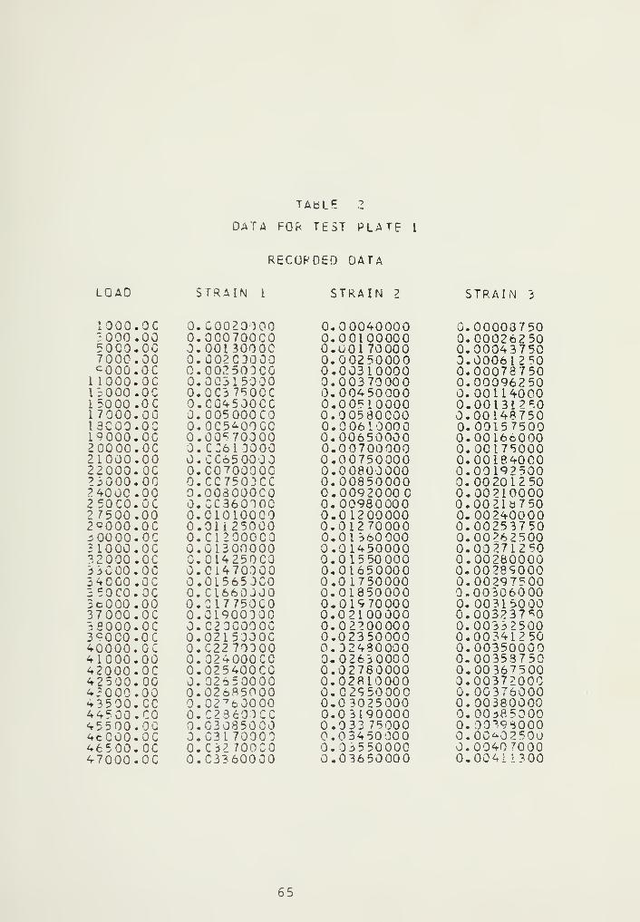
TAbLE 2
OATA FOfc TEST PLATE i
RECORDED DATA
LOAD STRAIN 1 STRAIN 2 STRAIN 3
1000,.OC 0.,00020000 0.00040000 0.00003750"000..00 0..00070000 0.00100000 0.0002625050C0..00 0.,001 3000C 0.00170000 0.000437507000,.00 0..00203000 0.00250000 0.00061 250c 000.,0C 0.,00250000 0.00310000 0.00073750
1 1000..OC 0.,00315000 0.00370000 0.000962501 3: 00..00 0. , 0C3 75OCC 0.00450000 0.001140001 5000.,oc 0,.C04500CC 0.00510000 0.001312*017000.. 00 0.,0 05 000 CO 0.00580000 0.0014375013CG0..oc 0..OC5400CG 0.0 061000 0.0015750019000..00 0.,00570000 0.00650000 0.0016600020000,.00 0. , C36 1 30 0.00700000 0.001750002 1000,.00 0. , CC650000 0.00750000 0.0018400022000..00 0..C070000C 0.00800000 0.0019250023000.,00 0..CC7503CC 0.00850000 0.0020125024000..00 0.,00800000 0.0092000C 0.002100002 50C0.,oc 0. CC360300 0.00980000 0.002137502 7500,.00 0. 01010000 0.01200000 0. 002400002 C 000,.00 0,.01
i
25000 0.01270000 0.00253750^OOCO..oc 0. , CI 2000 CO 0.01 360000 0.0026250031000..00 0.,01300000 0.01450000 0.0027125032000,.00 0. C14250CO 0.01550000 0.002800003 3000
.
.00 0.,01470300 0.01650000 0.00289000240G0,.00 0.,01565300 0.0 1750000 0.00297500350CO..00 0. C1660J00 0.01850000 0.003060002c 00..00 0.,31775000 0.01970000 0. 0031500037000.,oc 0.,01900300 0.02100 000 0.003237 c;0
39000..oc 0. C23C000C 0.02200000 0.00332500390C0,.oc 0.,02153300 0.02350000 0.0034125040000..oc 0,,C22 70300 0.32430000 0.0035000041C00..00 0. 024000CC 0.02630000 0.0035875042000,,oc 0..025400CO 0.02780000 0.003675004 2 5 00..00 0. 02650000 0.02810000 0.0037200043000,.00 0.,026^5000 0.0295000C 0.0037600043500.,cc 0.,02 7 60000 0.0 3025000 0. 0038000044500..CO 0. , C28603CC 0.03190000 0.00^8500045500,.00 0.,03085000 0.033 75000 0.003980004cC00..oc 0.,031 700CO 0.03450000 0.00^0250046500.,cc 0. . C 32 700C0 0.0^550000 0.0040 700047000..oc 0..C3360000 0.03650000 0.00 41 13 00
65


TABLE 3
DATA FGR TEST PLATE 1
CALCULATED STRESSES
LOAD NO, STRESS 1 STRESS 2 STRESS 3
1 2040.9? 4123.93 836.952 7300.45 10564.13 2687.92
1 3927. 23 13450.39 4518. 184 21785.23 26621 .02 6369.485 26621.02 33436.01 8233. 196 33945. C3 39090.82 10149. 377 39533.71 47660.69 12125. 278 47660.69 54038.90 14068.539 52655. 72 60786.64 16049.94
10 57131.38 63649.68 17040.2 911 59663. 62 66462.88 18000.0012 63648.68 70157.44 19011,9513 66462. 88 72007.06 20017.7914 70157.44 73826.44 20960. 5115 72007.06 75213.50 21921,9616 73826.44 76359.31 22859.2817 75401.88 7 71 7 P. 69 23738.41ie 77545.38 79048.06 25716. 8819 73519. 38 79503.00 26962.832 79048.06 80067.44 27776.0621 79691 .88 80555. CO 28624. 20; ? 80^35. 31 30956.19 29523. 2923 80642.44 31273.69 30632.9924 81009.06 81543.81 31353.2325 8 130 7. 3 8 81792.13 32998.4826 81606.56 8 2070.81 33945.0327 81911.88 82326.63 34814.5028 82135.00 82480.81 25662,36?9 92407.00 82696.06 36495. 0130 32582. 44 32875.25 3 7316.0931 82765. 75 83074.06 38103.46?? e2^55.75 83265.06 38871,3833 8 31 00.00 8 3 302.31 39 26 7. 1734 83145. GC 83472.69 33623. 26?5 83240. OG 83561.56 39985.9^36 8 3 36 3. cc 83751.63 40452. 34^ 7 83631.50 83956.81 41956.42? b 83729.00 84037.88 42592.41a o 8 3 3 41.38 84144.12 43228.47^6 33940. 50 84248.63 4 3 800. 11
66

TAaLE 4
DATA FCP TFST PLATF 1
STKESSES ANG STRAINS BASED ON LOAD(NOMINAL AND APPLIED)
LOAD NG. NCrt STRESS NCM STRAIN APP STRESS APP STRAIN
1 1291,99 0.00012217 925.93 0.00008756i 38 75.97 C.CCC3665 1 2777. 78 0.000262673 6459.95 0.0C061086 4629.63 0.000437764 9G43.93 0.0CG85520 6481.48 0.00061 2S95 116 2 7.91 C. 00109954 3333.33 0.00076*016 1^21 1.33 C.0C1343P9 1018 5.18 0.000963127 16795. 36 0.0C15882 3 12 03 7.04 0.001138236 1937C.P4 0.00183257 13838.89 C. 00131334c 21963.62 C.0C207692 15740.74 0.00148346IC 2 1 2 5 5 . 9 1 0.0C219909 16666.66 0.0015 760111 2^547.80 0.00232126 17592.59 0.0016635712 2533<5. 79 0.00244343 18518.52 0.0017511 213 27121.
7
J 0.0G25656C 1^444.45 0.0018386314 28473.77 0.0C268777 20370.37 0.0019262415 2971 5. 76 0. CC230994 21 296.30 CO 20 1 3 7916 21007.75 C.0C292212 22222.22 0.002-013517 32299. 74 0.00305429 23148.15 0.0021839119 j5529. 71 G. 0C335972 25462.96 0.00240730IS 37467.70 0.CC354297 26351 .85 0.00753^132C 36759.69 0. 00366514 27777.78 0.002&266921 4CC51.69 2.0C378732 28703.70 0.0027142*+2? 41343 .67 O.0G39C949 29629.63 0. 007801802 2 42635.66 C.0C403166 30555.55 0.002839362*r 43927.65 C.0C415383 31481.48 0.0029769125 ^5219.64 0.00427600 32407.41 0.0Q306h4726 465 11 .fc
3
0.CC43981 7 33 33 3. 33 0.0031520227 47802.62 O.0C452O35 34259.26 0.00323958?S +9C95.61 0.004642*52 35185. 19 0.0033271429 5 C 3 6 7 . 5 9 G.0C476469 361 11.11 0.00341469^0 51679.5 9 G.0CAfl8696 37037.04 0.003502^531 52971.57 G.0C500903 37962.96 0.003589813 2 542fc3.5 7 0.0C5 13120 38888.89 0.00367736*3 5 49 09.5 6 0.OC519229 39351.85 0.0037211434 55555.55 C.CC525337 39314.82 0.0037649235 5 j201.55 0.GC531446 40277.78 0.003808703b 57493.54 C.0C542663 41203.70 0.003896253 7 58 7 6 5.53 C. 0C555880 421 29.63 0. 00328381a o 5943 1.52 C.0C561989 42592.59 0.0040275939 60077.52 O.0C563097 43055.56 0.0040713640 60723.51 C.CC574206 43513.52 0.0041 1514
67


TABLE 5
HEURISTIC CATA FOR PLATE
LOAD NO. hEJ STRESS ACT STRESS RATIO
1 3236.41 3082.43 0.95242152 9963.06 8932.29 0.89654053 17051 .73 16188.81 0.94939434 23921.98 24203.13 1. 01175215 2993fc.44 30028.51 1.0030756o 37010. SI 36517.91 0.986679671 43602.05 43597.19 0.9^98835s 49832.90 50349.78 1.0193825Q 5 6 80 2.45 56721 .16 0.9985688
10 59392.75 60390.25 1.016794211 62790.42 63063.22 1.00434401 2 65118.95 66903.00 1.02 7396213 6 7 2 5 9.94 69234.94 1.029 3636L4 69619.06 71991 .94 1.034083415 71129.63 73610.25 1.0348740I ft 72239.56 75092.38 1.03949741 7 7 3393.19 76290.25 1 .03947261? 75520.56 78296.94 1.026762219 76269.94 79011 .19 1.035941120 76726.88 79557. 75 1.036894321 77141.38 30123.44 1.038656222 77530.56 80695.75 1.04082492 3 7 7 840.31 80960.56 1.040084824 78104.6° 81276.44 1.040608425 7 83 54. 3 8 81549. 75 1.040781026 78591.19 81838.69 1.041320827 78816.81 821 19.25 1.041899728 79033.06 82307.88 1.041435229 79241.75 82551 .50 1.041767130 79444.69 82728.81 1.041338031 7964 3.56 3 2919.88 1.041136732 79842 .44 83110.38 1.040929833 79941.44 8 320 1.13 1.040775334 80039.13 33308.81 1.040850635 801^4.69 83400.75 1.04075623 6 8031 6.56 83557.75 1.0 40 354 7
? 7 30480.94 8 3 794.13 1.04116733£ 305^4.69 83833.44 1.041322739 806?3.94 3 3992. 75 1.041793340 30690.88 84094.56 1.0421310
68


TABLE 6
DATA TOP TEST PLATE 1
STRESS AND E PRIME DATA
STRESS E PRIMP
7407.00 10575213.022222. CC 1057521 3.02S630.00 10575213.033^32.03 10575213.037C37. CC 1057521 3.04C741 .CO 1057521 3.044<*44. 00 1057521 3.048148. 30 1057521 3.051851 .CC 1057521 3.055555. CC 10575213. C59259. CC 10469792.0t?963.03 10476373.06 66 66. 00 10209191 .068519. CC 10061529.070^70.00 9995741 .072? 22. 00 9553174.07<tC74.CC 9 178934.0753?6.00 8511834.07o852. CC 3 0473 3 1 .077778.00 7529332.079629.00 6172791.080555. CC 555551 7.081481. CO 4723536.824-07.00 3832883. C8*259. CC 23021 58.08513 5.00 1755306.
69


TABLE 7
EXPONENTIAL CURVE FIT DATA FOR TEST PLATE 1
CALCULATED AC T,JAL RATIO E PkIMP
3 333.24 4C62.43 1.031367 10575213.099<=v.71 3932.29 1.119501 10575213.016666. 19 16188.81 1.029488 1057521 3.022332.67 24203.13 0.964035 10575213.029 c 99. 15 30028.51 0.999022 10575213.036665.62 36517.91 1.004045 1057521 3,043332. 10 4 3 597.19 0.993920 10575213.049998.58 506^9.78 0.983261 10575213.056303.92 56721 .16 0.992644 10521128.05Q254.07 603^0.25 0.981 1 86 10469840. C62o36. 71 6 3 0fc?.22 0.993237 i0481968.064639.37 66903.00 0.96ol65 10316608.06666 7.3
1
69^34.94 0.962914 10169520.068691. OC 71991.94 0.954148 10035024.070134. 75 73tl0.25 0.952785 9846504.072439.75 75C92 .88 0.964669 9765992.073951. 19 76290.25 0.969340 9609304.077623. 9-t 73296.94 0.993959 Q273Q9?.77762.31 7901 1.19 0. 9841 o4 8861480.081106.? 1 79557.75 1. 019*64 8940216.080709.^9 8 012 3.44 1.00731 7 86 73840.078747.31 8C695.75 0.9 75 861 8290497.08456P. 36 90960.56 1.0445 59 9564464.0£4273. 5C 81276.44 1.036833 8338224,08 12 15.31 81 549.75 0.995905 7908838.089169. 5C 81338.69 1.089576 3333666.091490.25 82119.25 1.1141 14 3322467.093155. 75 62307.68 1.131 796 3265074.094662.56 92551.50 I. 146721 6199579.096092.38 8 2 7 2 8.81 1. 161534 81313 7 6.098 106. c3 82919.88 1.133149 8106155.0980^5.66 83110.38 1. 179707 7947037.097cC3. 19 83201.13 1. 173099 7843431.09 7 4 5 7.0C 83308.81 1. 169827 7760348.0971 78.75 93400.75 1.165202 7671592.094533.94 83557.75 I. 131360 73681 15.089550.44 83794.13 1. 068695 693026^.06591 8.00 8 38 e 3. 44 1. 024254 6 6 45326.081616.50 839«=2.75 0.97170Q 6322C54.0C6940.19 84C94.56 1.271666 7735244.0
70


TA6LE 8
INVERSE RELATION CURVE FIT DATA FOk PLATE 1
CALCULATED ACTUAL RATIO F PRIME
3 5 3 3.33 3082.43 1.03139706 10575213.09999.99 3932.29 1. 119 53163 1057521 3.016666 .64 16188.81 1.02951527 10575213.033333.31 24203.13 0.9640ol80 10575213.029999.96 30028.51 0. 99904931 10575213.036666.63 36517.91 1.00407219 10575213.043333.28 43597. 19 0.99394667 10575213.049999.95 5C849.78 0.98328739 10575213.056483.56 56721.16 0.9958 1116 10517824.059225. C9 60390.25 0.98070610 10345792.062969.75 63C63.22 0.99851775 10473240.065492. 63 66903.00 0.978919 15 10262360.068060.94 69234.94 0.98304319 100331 1 2.070125.56 71991 .94 0.9740 7 520 97981 36.072301.69 73610.25 0.98222309 9563760.073892.00 75C92.88 0.93400313 9218848.075434.31 76290.25 0,98878050 8891288.078456. C6 78296.94 1.00 20 3 2 28 8014968.0P1636. 13 79011. 19 1.03322220 78 12931.032656.69 79557.75 1.03 895 187 7494142.081 766. 91 80123.44 1. 02050972 6867461 .084516.13 8G695.75 1.04734230 6886058.082465.81 80960.56 1.01859188 6123375,057972. 19 81276.44 1.08238220 6599799.086*15.25 31549.75 1.05966232 5968721 .083493.50 81838.69 1.02021930 51 706 5 3.0917*5.33 82119.25 L. 11722088 6025206.089704.50 82307.88 1.08986473 5391190.036649.56 82551.50 I. 04964161 4651 1 19,099399.13 82728.81 1. 20150471 60538*4.0
100299.69 82919.88 1.20959759 5847886.0101067.94 83 1 1C.38 1.21606327 5634937.0100872.25 8 32C1.13 1.21233995 54 595 13.0100324.38 83308.81 1. 20424652 5 2 44 5 2 4 .
99552. CO 8 3 400.75 1. 19365788 5006966.96550.31 83557.75 1. 15549133 4373? 77.093148. iS 8 3 79 4. 13 1. 11 163330 3720762-090520. 13 83883.44 1.0791 1777 3?97645.067869.94 83992.75 1.04616070 2881128.085556. 19 34C94.56 1.01733071 2511616.0
71


TABLF 9
DaTA FOR TEST PLATE .2
RECORDED DATA
LOAD STRAIN i STRAIN 2 STRAIN 3
3GCO.OC O.CC38000C 0.00090000 0.00026^006000.00 O.OOIdODOC 0.00175000 0.000524-009000. GC O.0O25OOOQ 0.00255000 0.00073t>0012000.00 0.CO35OO0C 0.00350000 0.001048001^000.00 0.00415300 0.0042500C 0.0013LOOO16000. OC 0.CC4500GC 0.00450000 0.0013900017000.00 0.004750CC 0.00490000 0.0014900018000.00 0. 00500000 0.00510COC 0.001570001°000.00 0.00530000 0.00550000 0.0016600020000.00 O.0C555OO0 0.00570000 0.0017500021000. CO O.C059O0OO 0.00600000 0.0018300022000.00 0.CC6250CC 0.C0650000 0.0019200023CCO.CC 0.C0O50000 0.00&90000 0.00^0100024000. OC G.CC700000 0.00740000 0.00210000?*OCO.CC 0.CC740OC0 0.00780000 0.0021300026000. OC C.CC770000 0.00795000 0.0027700027000.00 0.00815000 0.00845000 0.002360002PG00.0C 0.0C8600C0 0.00950000 0.0024400029000. GC 0.00^05000 0.01300000 0.0025300030C0G.0C C.CC9550CC 0.00955000 0.0026100031000. OC O.CIOLOOOO 0.01C10000 0.00^6950032000. CC D.CIC700C0 0.01070000 0.002730003iO0O.CC O.C113O0OO 0. 01130000 0.002870003^000. OC O.C1200000 C. 01200000 0.0029500035GCO.00 0.01260000 0.01260000 0.0030400036000.00 0.01230000 0.01280000 0.0031200037GCO.0C 0. 01400000 0.01400000 0.003210003S0G0.CC 0.C14300CC 0.01430000 0.0033100039C00.0C 0.C15600C0 0.01560000 O.C034000040C00.0C 0.0165000C 0.01650000 0.0034900041CGC.0C J.C17450C0 0.01745000 0.003590004?000.00 0.C1345000 0.01845000 0.0036300042rOC.CC 0.0I3950CQ 0.01895000 O.OO3730C04300C.OC 0.019500CC 0.01950000 0.00377000435CC.CC O.C2G00OO0 0.02000000 0.003820004^0G0.0C C.C2055OCC 0.02055000 0.0033660C4-+50C.CC 0.C2110000 0.02110000 0.00^91000^5000. OC 0.C213000C 0.0218000C 0.003960004-55CC.0C 0.02250JCC 0.02250000 0.00400000
72


TAril. p 10
Data FOR TEST PLATE 2
CALCULATED STRESSES
LCAO NO. STRESS 1 STRESS 2 STRESS I
1 8 3 73. 2C 9461 .90 2632.732 17322. ^6 19011.95 5431. 131 2fc6.11.C2 27077.47 8222.014 5131 6. C9 3 7316.09 I 109 7.235 442 37. 11 45223 .91 14040. 27c 4 7660. 5
9
47660.69 14945. 557 5CC96.C? 51558. o2 16078. 25e 5 26 55. 73 54038.°0 16 98 3. 749 ^c311.29 57901 .18 18 000.00
10 53295.82 596o3.62 19011.95n 619 21.43 6288^.39 19Q06. 3912 64738. 75 66462.83 20905. 23i a 66462.83 69292 .06 21394.64u 70157.44 71655.19 22859. 2815 71655. 19 73100.13 2 366 5.0616 72732. 75 73646.94 29203. 2917 74339. 13 751 1! .31 25354.2518 75401.88 76786.13 26078. 18IS 76130. 13 77429 .44 26894. 2320 7685<i. 00 76852.00 2 7 634.6121 7 7 54 5. 6 3 77545.88 2 3451.0122 780^0. Q4 78090.94 29312.452 3 76556. 38 78556. d8 3 035 9.892^ 79046.06 79043. 0-6 31495. 3025 7<9<t39. 50 79439.50 32751.2926 79566. 1 1 79566.13 3 3640. 7927 80301 . 88 80301 .33 3454^.8828 8C6 84. 81 80684.81 35518.27?9 6C991.63 80991.63 36376. 7530 81273.69 81278.69 37223. 7031 81531.25 81531 .25 3 312 5.5532 6 1779. 9 4 81779.94 3 8915. 2033 81 C J0.C6 81900.06 39355.7134 6 20 26. C '* 3 2026.63 39713.2135 82135.00 8 213 5.00 40170. S436 £2245. C6 82245.06 40605. 383 7 82343. 63 8 2 343.63 41059. 5838 d245i . ^4 d2^51 .44 41684.0039 82553.63 82553.63 42236. 54
73


TABLE 11
04 T 4 POR TEST PLATE 2
STRESSES ANO STRAINS BASFO ON LOAD(NCMINAL AND APPLIED)
LCAO NO. NCl^ STRESS NUM STRAIN APP STRESS APP STRAIN
j 2975. ?7 G. 0003665 1 2777. 78 0.00026257c 7751 .94 0.CCC73303 5555.55 0.00052534C I 1627.91 G. 00109954 8333.33 0.000738014 15=03.88 G.CC146606 11111.11 0. 001050675 19379.34 0.00183257 13888.89 0.00131 3346 20671. 83 0.0C195474 1491 4.81 0.001400907 21963.62 0.0C20769 2 15740. 74 0.001483468 23255.81 O.G021 C 909 16666. 6
o
0.001576019 24547.30 C.0C232126 17592.59 0. 001 6635 7
iC 25839. 79 0.0C244343 185 18.52 0.0017511211 2 7 131.78 0.0C?56560 1^444.45 0.0015386812 28423. 77 C.0C266777 203 70.37 0.0019262412 2^715.76 0.GC280994 21296. 30 0.00201379L4 31007. 75 0.00293212 22222.22 0.0021013515 32299. 74 0.0C2G5429 23 149.15 0.0021839116 33591 . 73 0.0C317646 2 4074.07 0.0022764617 348 83. 7 2 G.0C329863 25000.00 0.0023640218 361 75. 71 0.00342090 25925.93 0.002451 5719 37467. 70 0.00354297 26851.35 0.0025391320 38759.69 0. 00366514 27777. 78 0.0026266921 +0051 .68 C.0C3787^? 28703.70 0.002714^422 41343.67 0. 003909-^9 29629.63 0.0028018023 42635.66 0.00402 166 30555.55 0.0028393624 43927.65 0.0041538 3 31481.43 0.0029769125 45219. 6 + 0.00427600 32407.41 0.0030644726 465 11 .6 3 0.0C439817 33333.33 0.0031520227 +7803.62 0. 0C45203 5 34259.26 0.003239582 5 49095.61 0.0G464252 3 5 18 5.19 0.0033 271429 50397.59 0.OC476469 36 11 1.1 1 0. 0034146930 51679.59 0.0C4886P6 37037.04 0.0 3502253 1 52971 .5 7 C.0C500903 3 7 96 2.96 0.003589813 2 54265 .57 0.0C5131 20 38888.99 0.0036773633 54909.56 G.0C519229 3 93 5 1.85 0.003721 1434 55555.55 C. 00525337 39 PI 4. 92 0.00376492"3 C 5c 2 01 .55 0.00531446 40 2 7 7. 78 0.003603703
- 5694 7. 54 0.CC537555 40 74 0. 74 0.00 3 85247•3 7 57+93.54 C.0C5436o3 41203.70 0.0039962538 58 134.54 0.0C549772 41666.67 CO 039 +0 3
3 9 58785.53 0.0C55588C 42 I 2 9.63 0.00248381
74


TA3LE 12
HEURISTIC CATA FOR PLATE
LGAO NC- HEU STRESS
l 8 r>07.i42 18432.69a 27055.804 36 i46.945 45i85.59f 4794->.687 50703.1 I9 53Q7?.409 5696 1.63
10 59272. 75n 62381.7712 64579. 2413 6b534 .9414 68409.191= 70507.50
16 71515.0617 72523.5619 73560.19lc- 74516.83
^C 75iQ7.t I
21 75696.697? 76143.0023 76566.5024 76949.13-> s 77315.7526 77644. CO2 7 77902.0628 78137.0029 78J6C.3130 78573.25bl 78777. C6t? 78973.0633 79068.565 4 79162.56^5 79255.2526 79346.81^> 7 794? 7.4436 79527.19\c 79616.25
ACT STRESS
891718167268493 73164473047660508275334757106589796240265600678777090672377731897472576C947677976852775457809078556790487943979566R03018 068480991812788 15318177981900820268213582245623438245182553
RATIO
.55 1.0011683
.40 0.9656077
.25 0.9923657
.06 1.0266628
.50 0.98^9283
.69 0.9940766
.75 1.0024576
.31 0.9884134
.22 1. 0025339
.72 0.995056?
.41 1.0003300
.31 1.0155186
.44 1.0201769
.31 1.0365019
.63 1.0265236
.81 1.02341 75
.19 1.0303574
.00 1.0344443
.75 1.0303669
.00 1.02199 75
.38 1.0244234
.94 1.0255823
.38 1.0259886
.06 1.0277760
.50 1.0274677
.13 1. 0247555
.38 1. 0308046
.31 1
.
0326061.63 1.0335739.69 1.0344315.25 1. 03496 1
7
.94 1.0355415
.06 1.0353105
.63 1.0? 6 1786
.00 1.0363350
.06 1 .0365257
.63 1.0365339
.44 1 .0367699
.63 1. 3689 5
R
75


TAeLF 13
EXPCNEM l.L CURVE FIT DATA FOR TEST PLATE 2
CALCULATED ACTUAL RATIO E PRIME
P 9 8 C . 2 2 0917.55 1.007028 1057521 3.017960. -*5 18 lo7.40 0. 983608 105 75213.02694C.68 ? 6 C 49 • ?5 1.003405 10575213.035920. 90 37316. C6 0.96 26 12 1057521 3.04*901. 13 44730.50 1.003914 1057521 3.047394.54 4 766 0.69 1.004 9 06 1057521 3.050387.95 5C627.75 1.00 I 1 94 10575213.05 3 8 9 1.35 53347.31 1.010010 1057521^.0563ic. 59 c 7 106. 22 0.986073 10522144.058773.36 58979.72 0.996510 1047 7192.061 799.25 6 7 402.41 0.990334 10484688.06? 136. 2C 65600.61 0.962461 10352300.065375.59 6 78 7 7.44 0.963142 10302664.066329.19 7C9C6.31 0.942500 10 196312.068184.00 72^77.63 0.942059 10090152.069937.75 73139.51 0.955567 100 I 96 8 4.070971.25 74725.19 0.949763 9904200.072180.69 76C94.00 0.948573 9907360.073365.19 76779.75 0.955528 9714608.074866.88 76 6 5 2.00 0.974169 9646048 .0766 **6 • o 5 77545.88 0.988404 9603024.075090.06 78090.94 0.961572 9 3 53136.079031. 56 76556.38 1.006685 9452 776.080223.38 7"rC48.C6 1.014868 9379080.0812*2.94 79439.50 1.022701 9301968.08 2 9 8 6.13 79 56 6.1 3 1.042983 92695 76.81 423.31 60*01.88 1.013971 9055104.080038.63 80684.81 0. 991991 8857008.075945. C6 8 099 1.6 2 0. 93 76 90 3513272.037842.50 91278.69 1.080756 9045480.087266.00 81531.25 1.070337 8903968.055543.2 1 P1779.94 1.046013 3708328.0£4814. 50 81900.06 1.03 5 5 84 3619192.03 3 3 2 2.19 62326.63 1.015794 8492152.060374.50 22135.00 0.934653 3316697,077713.38 32245.06 0.944906 83 04327.092923.25 92343.63 1. 129602 9bl8984.093369." 1 32451 .44 1.132416 3790184.094337*44 8 2553.63 1. 142741 3736888.0
76

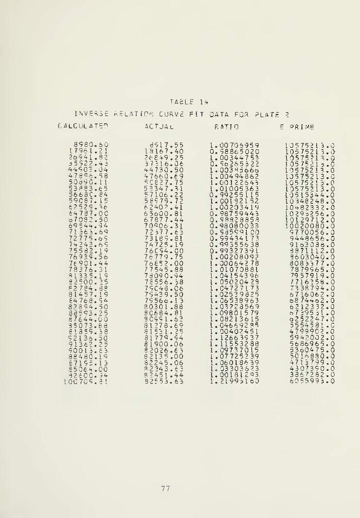
TABLE 1 4
INVERSE kELATCPN CURVE FIT DATA F3R PLATE 2
CALCULATED ACTJAl RATIO E PRIME
8980.50 8917.55 1.00 705959 1057521 3.017 961.21 13167.^0 0. 98865020 1057521 3.026941.82 26849.25 1.00344753 1057521 3.0^5922.43 37316.06 0. 96265322 1057521 5.04^903.04 ^4730.50 1.00385666 10575213.0478 c 6.58 47660.69 1.00494362 10575213. G50090. 1
1
5C827. 75 1.0012 2643 10575213.05 3 8 8 3.65 53347.31 1 .01005363 10575213.05663C. 84 57106.22 0. 992551 15 10 515344.059C87. 15 58979.72 1.00192152 10 348 2 48.0£7529.16 6
2
40?. 41 1.00203419 10^82332.064787.00 65600.81 0. 98759443 1029^256.0o7092.50 67877.44 0.9892885 3 10129 712.06954^.94 70^06.31 0.98080033 10020080.071 363.69 72 377.63 0.9359^1 CO 9770056.072775. 69 73189.81 0.994341 73 9448656.07t243.69 74725. 19 0.99355638 9163038.075582.19 76C94.00 0.99327391 8871112.076939.56 76779.75 1.00208092 3603040.076901.44 76852.00 1.000642 78 3083 3 7 7.078376.31 77545.88 1.01070881 7879965.08 13 3 5.19 73090.94 1.04154396 7957919.092500. '5 78556. 58 I. 05020429 7716258.0P2 784.38 79C43.C6 1.04727173 7338794.081457. 19 79439.50 1.02529325 6716062.064768. 94 79566. 13 1.06533963 68 74<*o2.082894.50 30301 .88 1.03223569 6212332.088593.25 80684.81 1.09801 5 79 o7395 31 .087644.00 90991.62 1.08213615 o2522^7.035073.83 3127 8.69 1.04669285 5554581 .061359.38 8153 1. 25 1. 00402451 47999C2.092136.30 8177<5.94 1. 12663937 5942002.091362.25 81900.06 1. 11553238 5686965.09001 3.63 8 20 26.6 3 1. 09737015 5360475.088480.19 82135.00 1.07725239 50 16 830.067195. 13 82245.06 1.060186 39 4713T99.09506^.00 82343.63 1. 03303673 4307390.082600.94 3745 1 .44 1.00181293 3367232.0
IOC 70 9. 3
1
92553.63 1. 219931 60 6055993.0
77

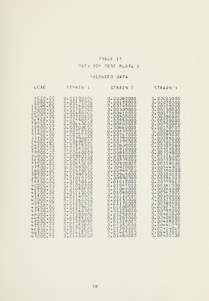
MfcLE 13
PATi FOR TEST PLATE 3
REGCkCEO data
LCAD <STRAIN I STRAIN 2 STRAIN 3
4CCO,,oc 0. CC100GOG 0.00080000 0.00033000SOOO,,00 0.,001 75 C 0.00155000 0.00070000
1 2COO..00 0..CC260000 0.00245000 0.001C50001 5COO..oc 0. CC3303CC 0.00300000 0.001300002CCOO..00 0..OC45O0CC 0.00410000 0.0017200024CCC,.00 0. G053OOCC 0.00500000 0.00200000265CO.,cc 0. CC C 900CG 0.00550000 0.00230000?65C0.,cc 0,.C0fr40G00 0.00600000 0.00^5000030500. , OC 0. C07C0C0 0.00660000 0.0027300031500,,oc 0. 007-5000 0.00695000 0. 00280000"*? C C0..00 0.,00755100 0.00747000 0.0028900C3 3 SCO,.CO 0. CC790000 0.00755000 0.0029500034QC0..oc 0.C08050GC 0.00775000 0.0030100034500. 0. 0C62530C 0.00800000 0.0030700035COO..00 0. CCS 500 CC 0.0C910000 0.00313000^5500,,cc .,C0S6OOCO 0.00830000 0. 003190003600C.,00 0. CC880DC0 0.00850000 0.0 3260 0036500..oc 0..C0910000 0.00875000 0.00332000^7000.,oc 0.,009^GC0C 0.C0900000 0.003380003 7=00..cc 0. CC9500CC 0. 00920000 0.0034400036000..oc 0. CC970000 0.00945GOO 0.0035000038500,,cc 0. CC990000 0.009o5000 0.0035300039GC0..oc 0. C 1010)30 0.00990000 0.003560003 9 5 00..oc 0.,010^00 00 0.01015000 0. 00^900040000,,00 0. C1C5000C 0.01045000 0.0036100040500. 0. G1080C00 0.01060000 0.0036400041C00.,oc 0.,011 10000 G. 01090000 0.0036700041500. i u c 0. Cll 400CC 0.0 11 20C0C 0. 0037000042000.,00 0. C1160000 G.011 50000 0.00373000425CC, , cc 0. C1200000 0.0 1170000 0.0038000043CC0.,00 0. Ci225GCC C. 01200000 0.0038700043 5 00.,cc 0.,ci2fcO")oa 0.01220000 0.0039500044CG0..00 0. C1300000 0.0 1250 00 0.004020004450C-CO 0. C12B50CC 0.0 1285000 0. 0040500045000.,00 0. , CI 3 200 00 0.0 132000 C 0.00408000* 5 5 C , CC 0. CI 350CCC 0.01350000 0. 00*4 I O^o46 000.,oc 0.,01290C00 0.01390000 0.00 4140 0046500..CO 0. 01 4250 CG 0.01425000 0.0G41700047000..00 0. C1450C0C 0.01480000 0.00420000
78


TAbLF 16
OaT4 FOP TEST PLATE 3
CALCULATED STRESSES
LCAP NO. iTRFSS 1 STRESS 2 STRESS 3
1 10564. LB 8573.20 3 390.362 190 11.9b 16757.51 7300.453 27540. 84 26168.48 11 119.554 3 5 4 2 1 . c 5 32213.81 13927. 2j>5 47660.69 43633.10 18675. 22c 5 6 3 11.29 52655.73 21785.237 6 1921.43 57901.13 24804. 508 6578?. 19 6 2883.39 26621.02o 70157.44 67133.13 ?° 31 ? .45
10 71130.81 69760.75 29523. 29i I 721 85.88 71900.88 30632.901 2 7 3465. 81 721 95.38 3149 5.3015 74003. 75 72916.44 32352. 5314 74631. 86 73826.44 33115.23lc
7 5 213.50 741 76.88 3 3 742.5 9lc 75401 .88 74763.83 34345. 5917 75736.25 75212.50 35034.3318 It 207. 3?. 75656.13 35614. 381*5 76 5 06.0 4 76052.13 36 18 7. 112C 76736. 13 76359.il 36754.5921 7 70 43.2 5 76716.56 37316. 0922 77306. 3£ 76982.69 37589.85? ^ 77545. 66 77306. :>8 37359. 3224 777 51.13 77601 .00 33125.554I > 7792*+. 50 77881 .88 3 8 301. 7526 78171.88 78008.50 38564. 3927 78406. 44 78251.44 38327. S7^3 786 29. 63 78482.00 39090.8229 787 72. 3 3 78701.75 39355.7150 79043.06 76843.00 39985. 94il 79 21 3. <5 79048.06 40643.9532 79439. n0 79180.94 41551. 812£ 79fc91 . 86 79375.63 42521.03
i *+ 79597. 5c 79^97.56 42943. 2835 79818. 19 7Q&18. 19 43365. 34?c 60006. J6 30006.06 46783. 5137 E0245. 3
L
80245.31 44125. 24Q 8 P043 5.31 8043 c .3i 4444 4. 0039 606 34. 6 1 3 06 84.31 44736. 47
79


TABLE 17
DATA FOR TEST PLATE 3
STRESSES AN? STRAINS(NOINAL AND
SAS CD fiN LOADAPPLIED)
LCAD NO. NOM STRESS NOM STRAIN APP STRESS APP STRAIN
1 4444. 44 0.0CC42027 3703. 70 0.000 3 50 2 27 8 8 8 8.39 0.0CC84Q54 7407.41 0. 000700453 13322.33 C.0C12608 I 11111.11 0.001050674 16666.66 C.0C157601 13 8 8 8.39 0.001313345 ????2 .2? 0.OC21O135 13518.52 0.001751126 26666.66 0.00252162 ????? . 77 0.0 0210 1357 29444.44 0.00278429 2453" 7. 04 0.002320248 21 666 .66 0.00299442 26.^88.89 0.002^95359 33386.89 C. CC320456 23240. 74 0.00267047
10 35000.00 0.00330963 29166.67 0.0027580211 36111.11 0.GC341469 300^2.59 0.0023455812 ^7222.22 C.CC351976 3101 8.52 0.0029331313 37777. 7e 0.CC357229 31481.43 0.0029769114 38233.33 0.0C362483 31944.45 0.0030206915 3 6 6 8 8.39 0.0C267736 32407.41 0.003064471c 39444.45 0.00^72990 32370.37 0.0 03 1032517 40C00.0C COO 3 78 24 3 33 33 3. 33 0.C03 15 20218 40555.55 0.00383496 33796.30 0.0031 95^019 4 1111.11 0.0C386750 34259.26 0.0032395820 41666.66 O.CC394003 34722.22 0.00323336£1 42222.22 0.0C39Q256 35185.19 0. 0033?71422 42777.78 0.00404510 35648.15 0.0033709223 4 3333.33 0.0C4C9763 3 1 I 1 . 1 1 0. 00341469?4 4^888 .39 0.00415016 36574.07 0.00345^4725 44444. 45 C. 00420270 37037.04 C.00^ c O22526 45000.00 0.00425523 37500.00 0.0025460327 455 55.55 C.C0430777 3796?. 96 0.0035 8 98 1
?q 461 11. 1 1 0. CC4360i0 38425. 9^ 0.00363 35829 -tot 06 .65 0.00441283 38888.89 0.00367736^0 47222.22 0.0C446537 393 5 1.35 0.003721 1431 47777. 78 C.0C451 790 39314.82 0.003754923 2 48233.33 0.0C457044 40277.78 0.0038087033 48888.39 0.00462297 40740. 74 0.0038524734 494.44.45 0.00467550 41203. 70 0.003396251 c 50000.00 0.00472303 41666.67 0.00*9400*36 5C555.55 C. CC478057 421 29.63 0.00398 38137 51111.11 0.0C48331O 42592.59 0.00402 75938 51666.67 0.00^38564 43055.56 0.004071 3639 5 ? P 7 ->
. ? ? C.CC49 3817 4 3 513.52 O.OOM 1514
80

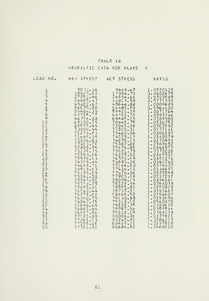
TAriLE 18
HEURISTIC CATA ECR PLATE
LOAD NO. HE J STRESS ACT STRESS RATIO
1 90 )C. 36 9463. t>7 1.05203257 18625.12 1 7 38 4.73 0.96024753 27292.46 263 54.66 0.98395894 34609.^2 3 381 7.88 0.97712925 45oC2.67 45646.86 1.00096896 54679.80 54483.50 0.99641007 5948^.39 59911.28 1. 00717648 63735.^7 64*32.78 1.0093746Q 66 736.88 68645.25 1.0235950
10 63150.7 5 70445. 75 1.03367521 1 699?7.44 72043 .38 1.030253212 7 33 9 6.44 72325.31 1.027213113 7127^.8 1 73460.06 1.0306537L4 71649.
W
7 42 29.13 1.036007915 72026.63 74695.19 1.03 7049 3
16 7241 3.21 75082.38 1.0368652I 7 72305.94 75474.38 1.0366573ia 73199.75 75931 .75 1.037322019 73590.56 76279.50 1.0365391£0 73974. 1
3
7657?.. 69 1 .035127621 74335.44 76883.38 1.034276022 74-648.^ 1 77144.50 1.0334337?t 7 4918.6 3 7 74 26.13 1.03 346 9 224 75153.83 7 7676.06 L. 0335598? * 75361.50 77903.19 1.033725726 75549. CC 78090. L9 1.033636127 757^3. 75 78328.94 1.034403328 75893.31 78555.31 1.035081929 76062.44 73737.31 1.035166730 76223.63 78945.50 1.035640721 7 6 390.75 791 30.88 1 .035369622 76547. 75 79310.19 1.03608703? 76698.69 79533 . 75 1.0 3696 3 5
34 76842.44 79597.56 1.0 35 85 3435 7698''. 56 79313.19 1. 2 6333836 771 23.00 3 0006.06 1.037382137 7 7 26 1.2 1 8 245.31 L. 038621938 77395. 06 80435.21 1 . 03 9 281
e
39 7752 i.8l 80634.81 1.04030 10
81


EXPONENTIAL
CALCULATFH
TABLE lo
CURVE FIT DATA FOR TFST PLATE
ACTUAL KATIO E PRIMF
9C69. 74 9468.67 0.957868 1057521 3.313139.46 1 7864.73 1.014244 13575213.02 7 209.2 3 26854.66 1.013203 10575213.034C11. 54 33817.88 1.0 05 7 26 1057521 3.045345.72 45646.38 0.993468 10575213.05441 8.47 54^83.50 0.993806 10575213.0^6731 . 54 5991 1. 23 0.946 9 36 10522496 .05934t,.6C 64232. 78 0.922494 10497184.062652.71 63645.25 0.912703 10484752.058 4 3 4. C 5 70445. 75 0. 829490 10392200.060239.10 7 2 04 3.38 0.836844 10392200.062144. 14 72825.81 0.853326 10392200.063071.67 73460. C6 0. 858584 10392200.06^999.20 74229.13 0. 862184 10392200.0£4926. 71 74695.19 0.869222 10392200.06565t.l9 75C82.88 0. 877087 10392200.066781.75 75474.83 0.884821 10392200.067709.25 7593 1.75 0.891 712 10392200.06 8 5 ? 7 . 9 4 76279.50 0.8 935 11 10390752.06 8 8 00. 13 76572.69 0. 893494 10382200.068720.19 76883.38 0.893824 10368976.06851°. 69 77144.50 0.888 186 10354576. C68481.50 77426.13 0.8844 75 10342480.063982.94 77676.06 0. 883085 10337563.070271. 1? 77903.19 0.902031 10342912.071824. 75 73090. 19 0.919767 103 51440.073026.38 73328.94 0.932304 10355488.073257.25 78555.81 0.932550 103473 84.072346. 13 78737.31 0.913829 10325243.071139.38 78945.50 0.9011 20 10299504. C
69764.13 79130.88 0.881630 10 2 716 3.068307.81 793 10. 19 0.8612 74 10242504.066851 .69 79533.75 0.840545 10213144.07 49 5 3. 5 6 79597.56 0. 9416 56 10305160.074819.31 79818.19 0.937372 10293536. C
7^fcl6.25 80006.06 0.932632 10 2313 36.074547.31 80 245.31 0. 928999 10270680.074805. 25 804^5.31 0.930005 10264048.01 5 7 3 G . 6 9 8Co84. 81 0.933599 10265504.0
82

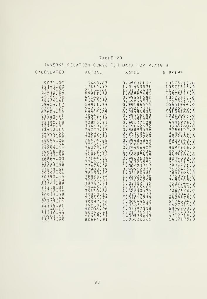
TAbLE 20
INVERSE RELATION CL'kVE FIT OATA FOR PLATF 3
CALCULATED AC":JAL RATIC E PRI"'
9071 .09 646 6.6 7 0.95 301 1 5 7 105 75213.018142.20 1 7 1 3 4 . 7 3 1. 01 4395 71 105 75 2 1 3.027213. 2^ 26f5*.66 1.01335430 105 752 1 3.034016.6? 23817.58 1.00587654 1357521 3.045355.50 45646.68 0. 99 36 16 32 1057521 3.054426. ol *44fi^. c 0.998955 73 1057521 3.
G
59*24. 1
7
5991 1.23 0.99136945 10 341 94 4.063861.27 64322.76 0.99267071 10326528.067604.25 63645.25 0.93433503 10103760.06 9 5 3 4.31 70445. 75 0.68 706 1 80 10020083.070926.06 72042.26 0.93451883 9 7 89744.072190. 13 72825.61 0. 991 ?7108 9 5 26 9 76.07275o.31 73460. C6 0.990426 72 9 398 760.073*12.19 74229. 13 0.93899436 0? 88 192.074066. 56 74695. 19 0.99 153412 9180^12.074423.88 75C82.83 0.99 12 2 2 93 3 9=8396.0750*6. Cfc 75474.88 0.99434843 8 6 00? 4 0.075631.94 75531.75 0.996051 55 8774958.07^89 5 .4*t 76279.50 0.9649650? 3 5 82S56.076658.88 7t 572.69 1.001 12534 351853b. C76873.68 7688 3.36 0.^99876 38 3323103.076364.00 7 7144.50 0.996 36 3 94 3 79030.07796c. 38 77426.13 1.00723553 31082 1 7.078005. ? c 77676.06 1.00423717 78 79821 .077673.63 77903. 1<= 0.69962050 76224?s 8 G79792.94 73090. 19 1.021 80431 7 8 3 7 3 8.080393.44 7P325.94 1.02635670 7750991 .030933. 19 76555.81 1.03026295 7653303.031242.88 78737. 31 1.03 132 1 2 5 7507544.Q81318.31 78945.50 1 .030056CO 7314439.081212.38 79130.88 1.02630424 70 67128.030955. 38 79310.19 1.02074337 o?33040.0303 <*C44 79533.75 1.01014233 6 5 09875.0796 32. 1? 79597. c 6 1 . 0004 46 3 2 61 74834.082739.31 79818. 19 1.03659630 6627 Jic.o82240. 13 80006.06 1.02762353 6 3 40 2 .
5 I 510.44 8C245.21 1 . 01 5 765 19 6013438.030901. 5fc 80435.31 1.00579643 5 7 17 7 15.065395.69 80664.81 1.05833535 6 4 27175.0
83

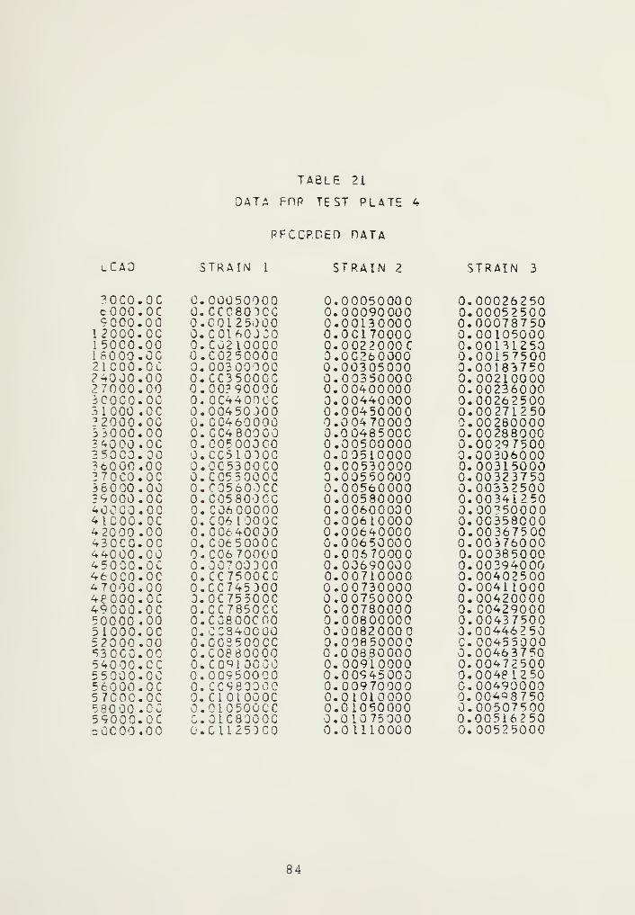
lCAD >;train i
^000,.OC 0. 00050000cOOO,.oc 0. CCC80TCC9000,,00 0.,00125000
12000,.00 0. 00160J201 50C0..00 0. CG21000018000..00 0,,0025000021C00. . oc 0. 0030000024000..00 0..CC35000C27000.,00 0.,CC?900003C0C0..00 0. GC4400CC31000
,
.00 0,,0045000022000..00 0. 004600003 3 000..00 0. CC4800003^0 00,.00 0.,005 0000025000..00 0. CQ5101QC36000..00 0, , OC 53 00 CO370CO.,0G 0. C055000C3 60 00..00 0. , C05 600CC29000..00 0,,005 800 0040000..00 0. , C060000041000.,oc 0. C06 1 OOOC42000 ,.00 0. , 00640000430C0.,00 0. C 06 5 OOOC44000,.00 0. , C06 70000450 00.. oc 0.,00700000460C0..oc 0. CC7500CC47000..00 0.,CC74530048000.,oc 0. 0C755O0C49000..oc 0. CC7850CC50000..00 0..C0800CO051000..oc 0. OC340COO52000,.00 0,,00950000S30CO..00 0.,C088000054000.,oc 0. CO^IOCCO55000..00 0. 0095000056000..oc 0. CC9 800057C0C..oc 0. CI 01000C5 90 00
,
r. 0.,01 0500 CC59000,,oc O m 01C8000C=0000..00 0.,01125)00
TABLE 21
DATA FRP TEST PLATE 4
RFCCP.DEf) DATA
STRAIN 2 STRAIN 3
0.00050000 0.000262500.00090000 0.000525000.00130000 0.000787500.0C170000 0.00105000O.O02200OC 0.00131250O.OC260000 0.001575000.00305000 0.001837500.00350000 0.002100000.00400000 0.002360000.00440000 0.002625000.00450000 0.002712500.00470000 0.002800000.00485000 0.002880000.00500000 0.002975000.00510000 0.003060000.00530000 0.003150000.00550000 0.003237500.00560000 0.003325000.00580000 0.003412500.00600000 0.003500000.00610000 0.003580000.00640000 0.003675000.00650000 0.003760000.00670000 0.003850000.00690000 0.003940000.00710000 0.004025000.00730000 0.004110000.00750000 0.00420000C. 00780000 0. C04290000.00800000 0.004375000.0082000C 0.004462500.00850000 C. 004550000.00880000 0.004637500.00910000 0.004725000.00945000 0.004812500.00970000 0.004900000.01010000 0.004987500.01050000 0.005075000.01075000 0.005162500.01110000 0.00525000
84


TABLE 22
DATA FOR TEST PLATE 4
CALCULATED STRESSES
LCAO NO. STRESS i STRESS 2 STRESS 2
1 5177. 36 5177.36 2687. 922 8373. 2C 946 1 .90 5441. 71i 13362.65 13927.23 8233. 194 17322. 86 18450.39 11119.555 2 23 59. 2 8 23859.94 14063. 5^6 26621. 02 2 7 540.34 1 7040.2 97 22213. PI 32877.03 19999.958 °7316. 09 37316.09 22859.289 4C947. 87 42236.54 25354. 25
10 46686.05 46686.05 27776.0611 47660. t>9 47660.69 29624. 2012 4 86 3 5. 2 8 49609.71 29523. 29i 3 50584. 14 51071.34 30495.0614 52655. 73 52655.73 31359.2315 54033. 90 54038.90 32993.48ifc 56311.29 56311.29 33945.0317 57901. 1
8
57901.18 34814.50L8 58712. 77 59712.77 35662.3619 60786. t4 60786.64 36495.0120 6 29 8 3. 3S 62883.39 3 73 16.0921 63648. 68 63648.68 38037. 1022 65782. 19 65782.19 38S71 ,3825 66462. 38 66462.88 39623.2624 67789.00 67789.00 40452.3425 70157. 44 69292.06 41422.8026 72007. C6 70593.13 42592.4127 71330.44 71306.13 43762.072P 721 85. ee 72007.06 44736.4729 732 83. 't4 73100.13 4561 3.8530 73826.44 73826.44 46 442.3831 75002. SI 74490.56 47295. 213 7 75213.50 75213.50 43143.0033 75736.25 75736.25 49000.70** *+ 7 6207.38 76207.38 49953. 323 c 76786. 1
3
7 6718.56 50705.9336 771 7d. 69 77043.25 51558.623 7 77545. 88 7 7545.88 524^6. 7333 7 79 2 4. 50 77924.50 53635,3239 781 71.66 73131 .03 54886. 77^0 78519.28 78406.44 55852.53
85

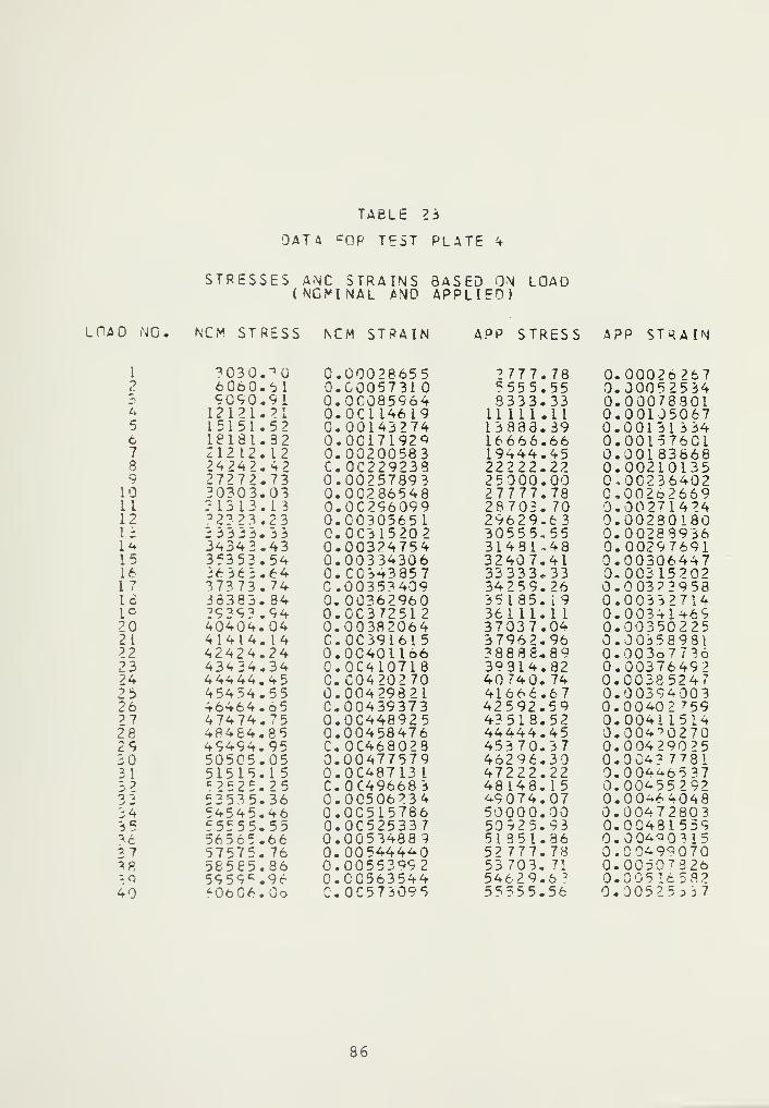
TAELE 23
DATA POP TEST PLATE 4
STRESSES A.NC STRAINS BASED ON LOAD(NOMINAL AND APPLIED)
LOAD NO. NCM STRESS NCM STRAIN APP STRESS APP STRAIN
1 3030.^0 0.00028655 2777.78 0.000262672 6060.61 0.0005731 5555.55 0.000525B4s~ 9090.91 0.0C085964 9333.33 0.00078901u 12 12 1.21 0.0CU46 19 11111.11 0.001050675 15151.52 0.00143274 13883.39 0.001 31 3346 ieiai.32 0.0C171929 16666.66 0.001576017 21212.12 0.00200583 19444.45 0.001838688 24242. 42 C.0C229238 22222.22 0.002101359 27272.73 0.00257893 2 5 000.00 0,00236402
10 30303.03 0.OC286548 27777.78 0.0026266911 3 13 13.13 O.OC296099 28703. 70 0.0027142412 323 23.2 3 0.0030565 1 29629.63 0.0023018013 3 3333. 33 G.0C3152O2 30555,55 0.0028993614 34343.43 0.00324754 314 31.48 0.0029769115 35353.54 0.00334306 32407.41 0.0030644716 36
3
t i. 6
4
C. CC3h3857 33333.33 0,003 1520217 37373.74 C. 00353409 34259.26 0.00372953Id 38383. 84 0.00362960 35185. 19 0.003 3 2714lc 29393.94 0.0C372512 361 11. 1 1 0.00341^69
20 40404.04 0.00382064 37037.04 0.0035022521 41414. 14 C.0C39161 5 37962.96 0.0 035 898
i
22 42424.24 0.00401166 38888-89 0.0036773623 43^34.34 0.OC41O718 39314.82 0.0037649224 44444.45 C. 00420270 40740. 74 0.0C38 524725 45454.55 0.00429821 41666.67 0.0039400326 46464 .65 G. 00439373 42592.59 0.00^02 7 5927 47474.75 0.0C448925 43518.52 0.0041 151428 48484.85 0.00458476 44444.45 0.004^027029 49494.95 C.0C468028 45370.37 0.0 04 2902530 50505.05 0.00477579 462 9 6.3 0.004? 773131 51515.1
5
0.0C487131 47222.22 0.00*4653732 c ? C
2C . ? 5 C.0C49668 3 48 148. 15 0.00^55292
a -5 53535.36 0.00506234 '+9074.07 0.00-6404934 54545.46 0.0C515786 50000.00 0.004729033 5 55555.55 0.OC525337 50925.93 0.00431 559^c 56565.66 0.00534889 51 351.96 0. 004^0^1537 57575. 76 0.005444^0 52 777. 78 0.00^9^070^fi 58585.86 0.00553992 53 703. 71 0.0050^32639 5959^.96 0.CC563544 54629.6? . C 5 1 6 5 3 2
40 A 0bG6. Go C. OC573095 55555.56 0.005 25 337
86


TABLE 24
HEURISTIC CATA FOP PLATE
LCAD NO. HEU STRESS ACT STRESS RATIO
1 4476.56 5 177.36 1 . !5o54952 9102.02 3917.55 0.9797328-* 13934.45 13644.94 0.9792230I 1833 4.5 2 17336.63 0.94967265 23544.33 23359.61 0.9921544c 27552.80 27080.93 0.98287377 32684.67 32545.42 0.99573958 37021 .68 37316.06 1.00795089 40968.39 41592.19 1.01521 30
1C 46057.01 46686.03 1.01365661 1 47465.57 47660.69 1.004110312 48873.98 49122.47 1.005084013 50232.17 50827.72 1.010849014 51e>90.46 52555.72 1.018672915 53445. 73 54038.88 1.01 1097916 5S363.33 56311 .28 1.017029817 5e.709.91 57901 .16 1.021005618 57836.13 58^12.75 1.015156719 59034.^0 60786.63 1.029682220 6 5 6 2.35 6 28 83.38 1.03832442 1 o2186.71 63648. 06 1.023508122 634?0.46 65782.19 1 .037239123 64483.41 66462.88 1.030696924 65498.16 67789.00 1.034975125 66484.56 69724.75 1.04873562e> 67446.69 71300.06 1.057131327 68399.25 71568.25 1.046330528 6964C.25 72096.44 1.035268829 70524. C6 73191.75 1.037826530 71045.38 73826.44 1.039144531 71551.44 74746.69 1 .0^4655832 72059.7 5 75213.50 1.0*376513^ 72583.56 75736.25 1.043435134 73114.19 76207.33 1.042 305 935 73641.06 76752.31 1.042248 7
36 741 52.75 77113.44 1.03992653 7 74597. 1 3 77545.88 1. 3 952 3
3
3 8 7 49oi.31 77924.50 i. 039522239 75265. 19 78151 .75 1.03 8 35 1 I
^0 75525.38 7 8462.8 8 1. 0383937
87


TABLE 25
EXPONENTIAL CU3VE PIT DATA FOR TEST PLATF 4
CALCULATE? ACTUAL RATIO E PRIME
4584.64 5177.36 0.885516 1057521 3.09169.29 8917.55 1.023229 10575213. C13753.93 13644.94 1.007987 1057521 3.018 3 3 8.57 1 7 686.63 1.025267 10575213.022923.21 2 3359.61 0.931319 10575213.027 507.86 2 7080.93 1.015764 10575213.032092.52 32545.42 0.986084 10575213.0366 7 7.16 37316.06 0.982879 1057^213.0A1261. ao 4 1592. 19 0.992057 10575213.045846.45 4-6686.03 0.962016 10575213.047374.66 47660.69 0.993999 10575213.048902.86 49 122.47 0.995530 10575213.050431.09 50827.72 0. 9^2197 10575213.051959.31 52655.72 0. 9 36 7 74 10575213.053487.52 540:>8.98 0. 989 7 97 10575213.055015.73 5631
1
.28 0.976993 10575213.056031.21 57901. 16 0.967705 10522496.057^97.38 58712.75 0.977596 10507792.058625.37 60786 .63 0.964445 10479984.059003. 38 6 2 88 3.38 0. 93 8 2 99 103721 1 2.061674.13 63648.66 0.968973 10483^76.063039. 70 65732.19 0.958309 10471360.063228.64 6 6 46 2 . 8 8 0.951 3 38 10354336.0o4539.36 6 7789.00 0.952062 1 3 40 2 .
65450. 54 69724.75 0. 938699 10 292632.066260.31 713C0.C6 0.92 93 23 102 3 8184.066967.69 71563 .25 0.935716 10177334. C6773 l.CC 72096.44 0.939450 1012 3 2 8.068442. 94 73191. 75 0.935118 10067256.06Q242.38 73826.44 0.937903 100 199 12.070365. 81 74746.69 0.941 390 99 99456.070535. 19 75213.50 0.937800 9906846.071235.38 75736.25 0.940572 9857280.071897. 13 76207.36 0.943440 9806472.073100.
l
c 76752.31 0.952417 9796960.073093.38 7 7113.44 0.947868 9700280.073934.25 77545.88 0.954071 9670308.0746 12.3 6 77924.50 0.957492 9623456.075 7 2 5. 38 76151 . 75 0.968 953 961 1528.07o072.5fc 76^62.68 0.969536 9547296.0


T AbLE 26
INVERSE RELATION CURVE FIT DATA FOR °IA T E 4
CALCULATED ACTUAL RATIO E PRIMF
4 3 24.,£4 5 177,,36 0. 98555497 10575213.0
9169. , o8 8 917, 1.02827263 10575213.013754. 32 li<:44,,94 1. 00803069 1057521 3.018339.,36 1 7886,.63 1.C2531147 10575213.02? c 24. 21 2^359..61 0.981 36085 10575213.02 7 509.,05 27C80.,93 1.01530811 1057521 3.032093. 39 32545..42 0.93612630 10575213.036676. 74 37316,.06 0. 93292100 10575213.041 26b. 56 41592.. 19 0.99209934 10575213.045F48.,42 4 668 6
,
.03 0.Q8205864 1057521 3.047376. 71 47660,.69 0.994041 56 105 752 1 3.0<t3904.,96 49122,.47 0.99557257 10575213.050433.,27 50827..72 0.99223936 105 75213.051^61. ,
c 5 52655,.72 0. 98681676 1057521 3.053439.,82 5*038,.83 0.9P983967 10575213.055019. , 11 56 311..26 0.97703522 10575213.056395,,03 5 7 9C1.. 16 0.97393300 10513536.57850.,66 53712,.75 0.98531637 10493536. C59965. 69 60786,.63 0.970043 84 10343816.060947.,13 6 2883..36 0.96 7618 70 10476816.062390.,37 6 3 6 4 3..66 0.93023075 10484264.063473.,04 65182. . 19 0. 96489704 103 39^-24.0o4828.,26 6b*t
2
..86 0.97540587 10^89160.066l c 3.,75 67789,.00 0. 97587734 1J231808.067238.,25 69724. . 75 0.96505541 101 18192.0fc3504.,o9 71 300..06 0.96079421 10034208.069936. 66 7 15c 3..25 0.97720528 10017400.070660.,94 7^C C 6,.44 C.9eC03913 9796838.071703.,56 7319 1..75 0. 9^966725 9675440.0724M .,3 I 73626.,44 0.981 23907 94 743 6 0.07327-+,,88 74746..69 0.93030931 9307203.073909.,38 75213,.50 0.98266101 9093440.074762. , Jl 75736. , 25 0. 98714036 3944864.07 5 5 7 1,,6*5 It 207 .33 0.99165845 8790600.7592C.,91 76752..31 0.989166 44 3525984.07679C.
, sc 77113,.44 0.99592888 94018 7 2.076863,,l c 77545,.88 0.991 19633 30 83 99 9.077961 ,,38 77924.^0 1 .00072956 30 28 986.077911.,68 7815 I.. 75 0.99693060 76 c 6933.079768,,38 78h62 .88 1.01663730 7820689.0
TABLE 27
EXPONENTIAL CURVE FIT DATA
PLATE NO. EXPONENT CORRELATION
5 .0542.0181 .0952 .210
-36.3 2-1 54.53.0146. 590
89


APPENDIX B
FINITE ELEMENT ANALYSIS DATA
TABLE 28
COMPUTER CATA FOR PLATE 1
APPLIED LCAO ANC RESULTANT STRESSES(NOTCH ROOT, APPLIED, AND NOMINAL STRFSSFSJ
LCAO NC
1
2a~*
456789
IC1112131415161718192021222324252fc
27282920
OAD (1.BS) NOTCH ROOT NGMI NAL APPL IED
5147.,94 187C4.00 6651 .03 4766.6 1
10295, , 68 37360.00 1330 2. 16 95 3 3.2115443..81 55 c 68.00 19953.25 14299. a?2C591,,75 767C8.00 26604. 33 19066.43216C7,,50 77392.00 27916. 66 20006.9422623..24 77680.00 ?9??8. 99 20947.452 3 6 3 8.,99 77912.00 30541. 33 21887.9524654. , 7 3 78126.00 31853.66 22928.462567C..43 78412.00 33165. 99 23768.9626686.,23 7 8 704.00 3447 8. 33 24709.4727701
,
,97 78965.00 35790.66 25649.972 6 717.,72 79216.00 37103.00 26590.4329733.,46 79479.00 3841 5. 33 27530.98JC749..21 79740.00 39 72 7.66 28471.4931 764.,96 80C06.00 41040. 00 29412.003273C. , 7C 8C257.00 42352.33 30352.5033796.,45 80728.00 43664.66 31293.0134ei2,,20 81C82.00 44977.00 i2 23 3 . 5 ?
35927..94 8 1426.00 46289.33 33174.0236643,,69 81784.00 47601 .66 34114.53^7859. , 43 82354. OC 4891 4. 00 35055.033 8975..13 82959.00 50 2 2 6. 3 3 359^5. 5439890, , 93 83536.00 51538. 66 36936.04->C906.,67 84C97.00 52851. 00 37876.554 19 2 2.,42 84640.00 54163. 33 38317.0542926, , 16 85 157.00 55475.66 39757.56**3Q*3,,91 8575o.00 56783.00 40693.0744c 6 9.,66 86445.00 58100. 33 41638.574 59 8 5.,40 871C8.00 5941 2. 66 42579. 0847C01.,15 87756.00 6072 5,00 43519.58
rf turf-
90


TABLE 29
COMPUTER DATA FOP PLATE I
CALCULATED STRAINS
LCAO NO. NOTCH ROOT NOMI NAL APPLIED
1 0.001768662 0.0C3532793 0.CC529237* 0.007253565 O.C07845576 0.008566287 0.009146858 0.009682389 0.010396C9
10 0.0111238111 0.011781^512 0.0124iJC715 0.C130682214 0.0137213615 0.C14387C216 0.015265 3817 0.0161938018 0.01707Q&719 0.C179405220 0.0188^64021 0.0202628022 0.C217768023 0.0232207224 0.C246246C25 0.C259834426 0.C272772127 0.C2&7761928 0.C30500392<* 0.C321595220 0.03378112
0.0006289?0. 00125786C. 001886790.002515720.0026 39820.002763920.002888010.0030 I 2110.0031 3620C. 00326030C. 003384390.003508490.003632580.003756680.00388077C. 0040 04870.0041 2896C. 00425306C. 004377150.00450125C.0C4625;>40.004749440.004673530. 0049 9 7630.005121720.00524582C.0053O99IC. 005494010.0056 1810C.0C574220
0.000450730.000901470.001352200.001802940. 001891 970.001980810.002069740. 002158680.002247610.002336550.002425430.002514420. 002603350.002692290.002781220.002870160.002959090.003048030.003136960.003225890. 003314330.003403760.003492700. 003581630.003670570.003759500.0038434^0.003937370,004026310.00411524
91


TABLE 30
COMP'JTFR CATA ^CR PLATE 2
APPLIED LCAC ANC RESULTANT STRESSES(NOTCH ROOT,APPLIFD, AND NOMINAL STRESSES)
LCAD no. LOAD (LBS) NOTCH ROOT NOMI nal APPL I 60
i 56S7.71 17654.00 7361 .39 5275.66I I 1395.43 35264.00 14722. 73 10551.323 17C93.14 52831.00 22034. 16 15326. 384 2279C.36 7C585.00 29445. 55 21 102.655 23667.43 73953.00 30578. 07 21914.296 24544.00 76903.00 31710. 59 22725.937 2542C. 57 77 315.00 32843. 1 1 23537.573 26297. 14 77^86. CO 33975.o3 24349. 209 27173.71 77619.00 35108. 15 25lo0.84
10 280 5C.28 77780.00 362 40. 6 7 25972.4811 28926.85 77957.00 37373. 19 26784. 1212 29803.42 78109.00 33505. 71 27595.761 3 30679.99 78268.00 39633. 23 23407.4014 31556.56 78431.00 40770.75 "'9 2 19. 0415 3 2433.13 78590.00 4190 3. 2 7 3003 0.6 816 23309.70 73815.00 43035. 79 30842.3217 341*6.27 79C49.C0 44168. 31 31653.9618 35062. 34 79270.00 45300. 83 32465.6019 35939.41 79477.00 <+6433. 35 33277.2?20 3681 5.98 79706.00 47565. 87 34088.8821 37692.55 80 139.00 48698. 39 34900.52> ? 38569.13 80521.00 49830.91 35712. 1523 39445. 70 8CE83.00 50963. 43 36523.7924 403 2 2.2 7 81228.00 52 09 5.9 5 3 7 335.4325 41198. 34 315 5 9.00 53228.47 38147.0726 42C75.41 81870.00 54360. 99 38953.7127 42951 .98 82224.00 55493. 51 39770.^523 43828. 55 32695.00 56626. 03 40581.9929 44705. 12 83 117.00 57753. 55 41393.6330 45581.69 8 3 518.00 58891 .07 42205.27
92


TABLE 31
COMPUTER OATA cqr p|_AT^ 2
CALCULATED STRAINS
lcao ni NCTCh r^OGT NOMINAL APPLIED
1
22<567P91C11121314151617Id192021222324?^2627?829?0
0.0O.CO.C0.0O.CO.C0.00.0o.o0.00.00.00.00.0O.CO.CO.C0. cO.CO.CO.C0.00.00. cO.C0. c0. c0.0O.CO.C
01669360333^59C499574060 7 4^706 99 3C5C72 72COC765268cecsoac0841363098165309259470963984100:>77310445631C8435311 406561199216125452C130o321136362814 7198415675 7910581661 7445C318 2 7 3 3 41905161199374821116 1422172182317567
0.000696100.00139220C. 002088290.00278439C.0C28914 C
0.00 299858C. 003105670.0032 12760.0033 i9850.00342694C. 003534040.00364113C. 00374822COO 38 55 31C. 00396240C.004C69500.0041 705Q0.0C428368C.CC4390770.00449786C.C0460495C. 004712050.0048 1914C. 0049 26250.005033320.00514041C. 005247510. 00535460C.0C5461690.00556878
0.000493870.000997740. 001496610.001995430.002072230.002148980.002225730.002302480.00 2379230.002455980.002532 730.002609480.002686220.002762970.002339720.002916470.002993220.003069970.003146720.003223470.003300220.003376 970.003453720.003530470. 003607220.003683960-003760710.00383 7460. 003914Z10.00399096
93

TABLE 32
fQMPJTER CATA FOR PLATE 3
APPLIED LGAC AND KESLLTANT STRESSES(NOTCH ROCT,AFPLlEDt AND NOMINAL STRESSES)
LOO NC
567
aQ
1011121?14151617IS192021
2324252627282930
74971499422491299863068C3 13 7 2320643275fc3344634140346323552436216J69CS3760036292389843967640368410604175242444-»313643828
4521245904^6596472884798C
LBS) NOTCH ROOT NOM IiMAL APPLIED
.00 17411.00 3330. 00 6941.66
.00 34771.00 16660.00 13883.33
.03 52C83.00 24990. 00 20825.00
.00 69610.00 33320. CO 77766.67
.03 72000.00 34088. 92 28407.43
.05 7 39 13.00 34 85 7. 84 29048.20
.08 75802.00 35676. 76 79688.96
. 11 77200.00 36395.68 30 329.7 3. 14 77251.00 37164.59 30970.50.16 ^7449.00 37933. 52 3161 U ?6. 19 77549.00 38702.43 3225 2.03.22 77646.00 39471 .35 32892.80.75 77741.00 40 240. 27 33533.56.27 776^3.00 41009. 19 34174.33.30 77944.00 41778. 11 3481 5.09.33 78C91.00 42547. 03 35455.36. 36 782C8.00 43315. 95 36096.63.3 8 78323.00 <t4 08 4. 87 36737. 39.41 78434.00 44 85 3. 79 37378.16.44 78542.00 45622. 71 38018.93.46 78649.00 46391 .63 38659. 6Q.49 76 766.00 47160.55 39300.46.52 7888G.00 47929.46 39941.27.55 78991.00 48698. 38 40 5 8 1 . 9 9.57 791C3.00 49467.30 41222. 75.60 79 218.00 50236. 22 41863.57.63 79^73.00 51005. 14 42504.29.66 79532.00 51774.06 43145.05.66 79686.00 52542.98 43765.32. 71 7S636.00 5331 1 . 90 44426.59
94

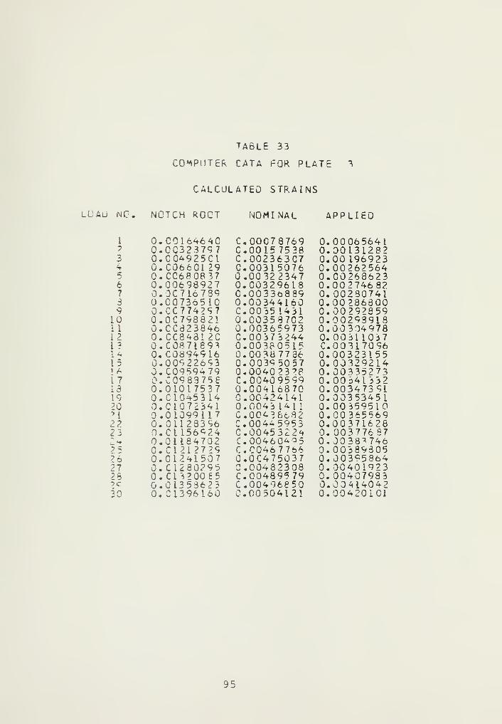
TABLE 33
COMPUTER CATA FOR PLATE 3
CALCULATED STRAINS
LOAD NC
1
?
3456739
1011121?1415i *i 7131920?12?232 475262726X30
NCTCH ROCT
0.C016464C0.CC3237970.CC4925CI0.C06601 290.CC6808370.006989270.3C7167890.C07365100.CC7742970.0C7988210.CC8238460. CC8431 2CO.C08718930.C08949160. 009226^30. 009^94790.C09837560.010175370.010*5314
. C 1 7 2 3 4 l
0. 010991 170. 011283S60.C1 1569240.011847320.C1 21 27290.012*15070. C1280295
. C 1 3 2 00 6 50.013536230. C1396160
NO MI NAL APPLIED
C.0007C.0015C.00230.00310.00320.00320.00330.0034C.00350.00350.0036C.00370.00380.00 380.00390.0040C.00400.00410.00 420.004 30.0043C.0044C.0045C.0046C.C0460.OC470.0048C.0048C.00490.00 50
8769753863C75076234796185889416014318 7025973324405157736505723?P95996870414114116682595332240^95776650372308957968504121
0.000.000.000.000.000.000. 000.000.000.000.000.coo0.000. 000.000.000.000.000.000.000.000. 000.000.000.000.000. 000.00.00
0656411312821969232625642686232746 822307412863002928592939183 0497831 10373170S632315532921433527334133 23473913534513595103655693 716 2 83776 9738^746389305395864401923407983414042420101
95

TABLE 34
COMPUTER CATA FOR PLATE 4
APPLIED LOAC AND RESULTANT STRESSES(NOTCH RGGTtAPPLl ED, AND NOMINAL STRESSES)
LCAD NO. LOAC (LBS) NOTCH ROOT NOMINAL APPL ied
1 11495.39 17350.00 11611. 51 10643. 882 2299C.79 34t45. OC 23223.02 21287. 773 34466. 18 5 1687. CO 34834.53 319 31.654 45981.58 69C74.00 46446.04 42575. 545 46 5 2 7. 51 69689.00 46997.49 43031.036 4 70 7 3. 4 5 7C7C4.00 47548.93 43586.527 47619.^8 71519.00 48100. 33 4409?. 028 H8165.31 72334.00 48651. 83 44 59 7.5 1
c 48 71 1.2 5 73148.00 49203.23 45103.0110 4=257. 18 74026.00 49 754. 73 45o08.501 1 4^803.11 75CC0.C0 50306. 18 ^61 1 4.0012 50349.05 75905.00 50857.63 4661 9.4912 5C394.98 76797.00 51409.07 47124.9314 5 144C.91 77196.00 51960. 52 4 7630.4315 51986.85 77247.00 52511.97 48135.9716 52532. 76 77285.00 53063.42 48641 .461 7 53078.71 77323.00 53614. 86 491M-6.9618 5 3624.65 77361.00 54166.31 49652.4519 541 7C.58 774C8.00 54 71 7. 76 501 57.9520 5 4 7 1 c . 5 2 77456.00 ^5269.21 50663.4421 55262.45 77499.00 55820.66 51 168.94?7 55808.38 77542.00 56372. 11 51674,4323 56354.32 77588.00 56Q23. 55 52179.9324 5690C.25 77633.00 57475. CO 5 2 6 3 5.422 ? 5 7*^6. 13 77677.00 58026.45 53190.912 6 5 799 2.12 77720.00 58577.90 53696.4]27 5 6 5 3 8 . C 5 77766.00 59129. 34 54 2 01.9028 5 9083.93 7783 2.00 59 6 3 0. 79 54707. 3929 5^629.92 77898. OC 60232. 2^ 5521 2.393 6C1 75. 65 77960.00 60782, 69 55 71 3.3 8
96
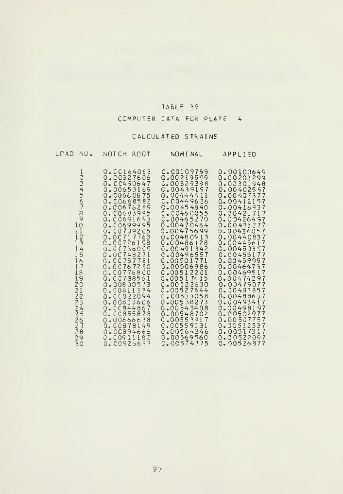
TABLE 35
COMPUTER CATA FOR PLATE 4
CALCULATED STRAINS
LfAD NO. NOTCH ROOT NOMI NAL APPLIEO
1 0.,CC164063 C.C0109799 0. 00100649y 0.,C03276Q6 C. 00219599 0.002012992 0. CC490647 C. 00329398 0.003019484 0.,00653169 C. 00439197 0.004025975 0,,00660875 0,004444 11 0.004073776 0,,C0fc68582 C. 0044 96 26 0.004121 577 0.,00676289 C. 00454840 0.004169378 0. C0683995 C.CC460055 0.004217179 0. C06916S3 C. 00465270 0.00426497
10 0. , C0699995 0.00470484 0.0043127711 0. C07092C5 0.00475699 0.0043605712 0. 0C717763 0.0048 09 13 0.0044083713 0. 00726198 0.00486128 0.0044561714 0. CC73oOC9 0.00491342 0. 004503 9715 0.0C748271 0.00496557 0.0045517716 0. CC757781 0.00501771 0.004599571 7 0. 0C767290 0.00506986 0. 0046473718 0. C0776800 0.00512201 0.0046951719 0. CC738561 0.00 5 1 7415 0.0047429720 0.,00800573 C. 00522630 0.0047907721 0.,00811334 0.00527844 0.00483857?? 0. CC822094 C.C0533058 0. 0048363723 0. 008336C6 0.00538273 0.0049341724 0. CC844867 0.00 543438 0.00498197?5 0. CC355879 0.00548702 0.0050297726 0.,00866638 0.00553917 0.0050 7 75727 0. CC878149 0.005591 31 0.0051253728 0.,00894666 0.0056*346 0.0051731729 0,,00911182 0.00569560 0.00 5 2 209 7
3 0. C092o6<=7 C.0C574 7 75 0. 00526377
97


LIST OF REFERENCES
1. Butler, C. L. , Software Design for a Fatigue MonitoringAcquisition System , Master's Thesis, Naval PostgraduateSchool, Monterey, California, September 1976.
2. Wetzel, R.M. , "Smooth Specimen Simulation of FatigueBehavior of Notches," Journal of Materials , March 1969.
3. Neuber, H., "Theory of Stress Concentration for ShearStrained Prismatical Bodies with Arbitrary NonlinearStress-Strain Law," Journal of Applied Mechanics ,
December 1961.
4. Impellizzeri , L. F. , "Cumulative Damage Analysis inStructural Fatigue," Effects of Environment and ComplexLoad History on Fatigue Life , ASTM Stp 462, January 1970.
5. NASA Technical Note D-5253, Elastoplastic Stress-Strain3ehavior at Notch Roots in Sheet Specimens Under Constant -
Amplitude Loading , by J . A. Crews, Jr., June 1969.
6. Naval Research Laboratory Report 7278, Finite ElementAnalysis of Notched Tensile Specimens in Plane Stress ,
by C. A. Griffis, 30 March 1971.
7. Home, M. H., An Investigation of Stress Determinationfor Aircraft Fatigue Life Estimation From In-FlightStrain Data , Master's Thesis, Naval Postgraduate School,Monterey, California, September 1976.
8. Atkinson, S.J., A Study of Spectrum Loading and Range-Pair Counting Method Effects on Cumulative FatigueDamage , Master's Thesis, Naval Postgraduate School,Monterey, California, February 1977.
9. Bathe, K.J., Wilson, E.L., and Iding, F.E., NONSAP,Structural Engineering Laboratory, University ofCalifornia, Berkeley, California, February 1974.
10. Bathe, K.J., ADINA, Acoustics and Vibration Laboratory,Massachusetts Institute of Technology, Cambridge,Massachusetts, September 1975.
98


INITIAL DISTRIBUTION LISTNo. Copies
1. Defense Documentation Center 2
Cameron StationAlexandria, VA 22314
2. Library, Code 014 2 2
Naval Postgraduate SchoolMonterey, CA 9 3940
3. Department Chairman, Code 6 7 2
Department of AeronauticsNaval Postgraduate SchoolMonterey, CA 9 39 40
4. Associate Professor G. H. Lindsey, Code 67Li 1
Department of AeronauticsNaval Postgraduate SchoolMonterey, CA 939 40
5. LT John Charles Garske, USN 1
2726 West UptonSpokane, WA 9 9 205
99


JUIW2 7087
Thesis 172278G225 Garskec.l An investigation of
methods for determin-ing notch root stressfrom far field strainin notched flat plates,
Thesis
G225
iiiHtJS2 U C 8 92 7087;
172:Garske
An invest ioat ion ofmethods for determin-ing notch root stressfrom far field strainin notched flat plates.
78

thesG225
An investigation of methods for determin
3 2768 002 01078 7DUDLEY KNOX LIBRARY


![[Credentials];[Notch JSC]](https://img.dokumen.tips/doc/110x75/5442a5f9b1af9f350a8b46f3/credentialsnotch-jsc.jpg)
