An Investigation into the Interest Elasticity of Demand

International Journal of Economics and Finance; Vol. 9, No. 3; 2017

ISSN 1916-971X E-ISSN 1916-9728

Published by Canadian Center of Science and Education

69

An Investigation into the Interest Elasticity of Demand for Money in

Developing Countries: A Panel Data Approach

Felix S. Nyumuah1

1 Department of Financial Management, Zenith University College, Accra, Ghana

Correspondence: Felix S. Nyumuah, P.O. Box SK 237, Sakumono Estates, Tema, Ghana. Tel: 233-243-671-295.

E-mail: [email protected] or [email protected]

Received: December 19, 2016 Accepted: January 17, 2017 Online Published: February 15, 2017

doi:10.5539/ijef.v9n3p69 URL: https://doi.org/10.5539/ijef.v9n3p69

Abstract

The issue as to whether the interest rate influences the demand for money in developing countries is still

controversial. The aim of this study is to attempt to resolve this controversy. The study uses panel data from

eight African countries to look at the interest elasticity of demand for money in developing countries. The

countries used in the study are Angola (ANG), Equatorial Guinea (EQG), Gambia (GMB), Guinea-Bissau (GBS),

Kenya (KNY), Mali (MLI), Nigeria (NGR) and Uganda (UGD). Overall, the study finds the interest rate to be

inelastic in the short run but elastic in the long run. This finding suggests that monetary policy is ineffective in

developing countries in the long run.

Keywords: demand for money, interest rates effects, monetary policy, panel data models

I. Introduction

Researchers have conducted a lot of studies into the demand for money over the past decades. This is because

understanding the demand for money in an economy is key to the formulation and implementation of monetary

policy. The success of monetary policy depends on the degree of responsiveness of money demand to the interest

rate. Researchers have often argued that the interest rate does not play a significant role in determining the

demand for money in developing countries because of the dearth of financial assets. The issue of whether the

interest rate influences the demand for money in developing countries is still controversial in the light of mixed

results obtained so far by researchers. For instance, the domestic interest rate is found to play a statistically

significant role in explaining the long-run demand for M1 balances in some developing countries whilst the

expected inflation rate shows a short-run impact in others (Simmons, 1992). Arize and Nam (2012) find the

domestic interest rates to have significant negative effects on the demand for money for seven Asian countries.

Econometric analysis of the demand for money from some earlier studies have found the interest rate to be

statistically insignificant (Terriba, 1973, Pathak, 1981). In addition to this controversy about the interest rate, the

use of more advanced statistical techniques in modelling demand for money is gaining popularity among

researchers. The purpose of this study is to use panel data techniques to resolve the controversy surrounding the

interest elasticity of demand for money in developing countries.

This paper computes the short and long run interest rate elasticity for a panel of eight sub-Saharan African

countries and argues that the interest rate is inelastic in the short run but elastic in the long run. Based on the

IS-LM framework, the study concludes that the economies of these countries will be in the Keynesian range in

the long run. Policymakers cannot safely rely on monetary policy to influence output and inflation in the long

run.

I obtain the interest elasticity coefficients of the money demand function by using a panel Fully Modified

Ordinary Least Squares (FMOLS) estimations for the long run and the estimates of fixed and random effects

error correction models for the short run. Panel unit root tests initially carried out show that all the variables

under study are integrated of order one. Pedroni cointegration tests also indicate that cointegration exists. The

Fully Modified Ordinary Least Squares estimates of the money demand function show that the interest rate

exerts a significant influence on the demand for money whilst the expected rate of inflation does not play a

significant role in explaining money demand in the long run. However, the error correction model representing

the short run dynamics of the money demand shows that the expected rate of inflation is statistically significant

and the interest rate is statistically insignificant in the short run.

ijef.ccsenet.org International Journal of Economics and Finance Vol. 9, No. 3; 2017

70

The literature which examines the demand for money in developing countries, using panel data techniques and

incorporating modern time series methods (e.g., Harb, 2004; Carrera, 2008; Hamori, 2008; Valadkhani, 2008;

Rao & Kumar, 2009), influences the conduct of this study. All the studies except Hamori (2008) were conducted

for Asian countries. Hamori (2008) used Pedroni Fully Modified Ordinary Least Squares (FMOLS) to analyse

the money demand function for Sub-Saharan Africa. The interest rate was significant with the correct negative

sign. Also, all the studies but Valadkhani (2008) estimated only a long run money demand function. Valadkhani

(2008) examined both the long run and short run determinants of money demand for six Asian-Pacific countries.

From the literature, there has been no study from Africa analysing both the long run and short run money

demand function within a panel framework. This study contributes to the literature in that, unlike the earlier

studies, it focuses on the issue of the interest rate influence on the money demand function in developing

countries by using data from Sub-Saharan African countries, and at the same time demonstrates by using a panel

FMOLS and an error correction model that the interest rate is inelastic in the short run but elastic in the long run.

This is because economic agents are not able to substitute money for financial assets as the interest rate rises.

However, in the long run, they are able to find more financial assets and adjust to equilibrium. Generating results

from Africa in this way provides more evidence to support the theory of demand for money for developing

countries. This study uses data from eight Sub-Saharan African countries. I chose these countries because

consistent time series data on all the variables included in the model were available.

The paper continues with Section 2 reviewing the theoretical literature of money demand and providing evidence

to show the controversial nature of interest elasticity of money demand in developing countries. This section

discusses the relationship between interest elasticity of demand for money and monetary policy. It demonstrates

that the more interest elastic the demand for money the less effective monetary policy is. Section 3 reviews the

advantages of panel data over pure cross sectional or time series data and specifies the fixed effects and random

effects models. It shows that panel data leads to efficiency in econometric estimates and improvement in

statistical inference. Section 4 describes the estimation techniques, estimates and interprets the results. Section 5

discusses policy implications and directions for future research.

2. A Review of Literature

This section reviews the theoretical underpinnings of the demand for money and the empirical evidence from

past researchers concerning the right opportunity cost variable in the money demand function of developing

countries. It further examines the effectiveness of monetary and fiscal policies using the IS-LM framework.

2.1 The Theoretical Literature

Fisher (1911) came out with the classical quantity theory which was the earliest attempt to formulate a theory of

demand for money. The classical quantity theory is expressed as an equation of exchange where the total money

supply determines the total amount of spending on final goods and services. Fisher assumes money is held only

for transaction purposes. With money market equilibrium, the supply of money is equal to the demand for money,

and the equation can be transformed into a money demand function where the amount of cash balances held is

purely a function of nominal income. Thus the interest rate plays no role in determining the demand for money

in this formulation.

As an improvement over Fisher’s theory, Pigou (1917) and Marshal (1923) developed the Cash Balance version

of the Quantity Theory. These neoclassical economists explicitly express the equation as a money demand

function showing the amount of cash balances held as a function of nominal income. They consider the possible

influence of wealth and the interest rate in the function through their influence on the velocity of circulation.

Keynes (1936), in his liquidity preference theory, showed that the amount of money held is inversely related to

the interest rate. Keynes distinguished between real and nominal values. According to Keynes, the interest rate,

which influences money demand appreciably, and real income determine the demand for real cash balances. To

further develop the Keynesian theory, Baumol (1952) and Tobin (1956) showed that the transactions demand for

money was also sensitive to the interest rate. Their optimum inventory analysis leads to the square root formula

which expresses optimal demand for real balances as a function of transaction costs, level of transactions and the

interest rate. Tobin (1958) explains the demand for money as aversion to risk. He argues that the individual will

diversify his portfolio by holding some proportion of wealth in money because doing so lowers the overall

riskiness of the portfolio. Given a person's degree of risk aversion, a higher expected return (nominal interest rate

plus expected capital gains on bonds) will cause agents to shift away from safe money and into risky assets. This

creates a negative relationship between the nominal interest rate and the demand for money. Friedman (1956)

refines the classical Quantity Theory and treats the demand for money like the demand for any other asset.

Wealth, according to Milton Friedman, can be held in the form of money, bonds, equity and real assets. The


71

demand for money is specified as a function of permanent income and expected returns relative to the expected

return on money. The demand for money is positively related to permanent income and inversely related to the

expected returns on the various assets relative to the expected return on money. Since real assets are considered a

form of holding wealth, the expected rate of inflation relative to the expected return on money is introduced as a

variable in the money demand function. Friedman, however, predicts a weak negative correlation between

money demand and interest rates.

The standard demand for money theories assume well-developed financial markets exist with financial assets

readily available. However, financial markets in developing countries are undeveloped. The interest rate is often

considered as an unsatisfactory measure of the opportunity cost of holding money, because the dearth of

financial assets limits the substitution between money and financial assets. The expected rate of inflation is

regarded a more appropriate measure, because of the likelihood to substitute physical assets for money in

developing countries.

2.2 Empirical Evidence from Developing Countries

As is obvious from the previous section it is believed that the expected rate of inflation and not the interest rate

should be the appropriate opportunity cost variable in the money demand function for developing countries.

Several studies have used the inflation rate as the opportunity cost of holding money; (for instance, Wong, 1977;

Suliman & Dafaalla, 2011; Bahmani-Oskooee & Bahmani, 2015). Further explanation given in favour of the

expected rate of inflation is that interest rates are regulated by the government and remain unchanged for long

periods of time. For these reasons, it is more appropriate to use the inflation rate as a proxy for the opportunity

cost of holding money (Tang, 2009; Bahmani, 2013). Laidler (1985) justifies the inclusion of the nominal

interest rate as own rate of money as well as the expected inflation rate. Arestis and Demetriades (1991) argues

for the inclusion of both variables since nominal interest rates can be considered as own-rate of money; and the

expected inflation rate is the return on real assets. Thus studies like Rao and Kumar (2010) and Abdulkheir (2013)

have included both the interest rate and the inflation rate in the money demand function.

Studies that have been carried out have used both single countries and panels of countries. For instance, Rao and

Singh (2005) in a study of the demand for money in India using unit roots and cointegration methodology,

showed that the interest elasticity of the demand for M1 is significant. Using a partial adjustment method (PAM),

Hossain (2006) found the interest rate to be statistically significant in the money demand function for

Bangladesh. Rao and Kumar (2007), using time series approach and the Gregory and Hansen technique for

structural breaks to estimate the demand for real narrow money for Bangladesh for the period 1973-2003, found

the interest rate elasticity to be significant and negative. Baharumshah, Mohd, and Masih (2009) also looked at

the demand for money in China. In the preliminary analysis, they found that the domestic interest rate elasticity

was insignificant even at the 10% significance level. This result could be due to the fact that interest rates

remained heavily administered. Kumar, Webber and Fargher (2010) estimated the demand for real narrow money

(M1) for Nigeria over the period 1960-2008.They found the interest rate elasticity to be negative and significant.

Dagher and Kovanen (2011) in a study of the demand for money for Ghana found the interest rate to be

statistically insignificant. Some other studies (like Herve & Shen, 2011; Sichei & Kamau, 2012), carried out on

single country basis, have found the interest rate to impact negatively on money demand.

Concerning panels of countries, Simmons (1992) used an error-correction model to examine the demand for

money for a panel of five African countries comprising the Democratic Republic of Congo, Ivory Coast,

Mauritius, Morocco and Tunisia. The empirical results indicate that the domestic interest rate influences the

demand for money significantly in the long run in the case of Ivory Coast, Mauritius and Morocco. He also

found that inflation exerted a significant influence on money demand in four of the countries. Singh and Kumar

(2012) using alternative time series techniques for 12 developing countries found for almost all the sample

countries that, the interest elasticities were well determined and significant. Abdullah, Ali, and Matahir (2010)

reexamined the demand for money in Singapore, Malaysia, Thailand, Indonesia, and the Philippines. The

inflation elasticity was negative. Narayan, P. K., Narayan, S., and Mishra (2009) estimated a money demand

function for a panel of five South Asian countries. The impact of the short-term domestic nominal interest rate

produced mixed results. For Bangladesh and India, the interest rate was negative and statistically significant.

However, the interest rate was negative but statistically insignificant for Sri Lanka. On the other hand, for

Pakistan and Nepal, the relationship while positive was statistically insignificant. Rao and Kumar (2009)

estimated the cointegrating equations for the money demand of a panel of 14 Asian countries

from1970-2005.The elasticity estimates were all significant at the 5% level. The interest rate elasticity carried

the anticipated negative sign. Some other studies which have applied panel data techniques in recent times are

Kumar, Chowdhury, and Rao (2010) and Rao and Kumar (2010). Kumar et al. (2010) found money demand to


72

respond negatively to the interest rate and Rao and Kumar (2010) found the nominal short-and-long-term interest

rates and the rate of inflation as robust proxies of the opportunity cost of holding money. It appears mixed results

have so far been obtained by various researchers regarding the relevant opportunity cost variable in money

demand functions in developing countries.

2.3 Interest Rate Elasticity and Monetary Policy

Monetary policy and fiscal policy are two main policies used in the stabilisation of economies. Monetary policy

is conducted by using the money supply or the interest rate as a policy instrument. A change in any of the policy

instruments will be expected to affect inflation and output. According to the Keynesian transmission mechanism,

money affects inflation and output indirectly through the interest rate. Expanding the money supply reduces

interest rates; the cost of borrowing for firms and consumers. This leads to increased consumption as well as

investment. There is therefore an increase in demand and a higher output gap resulting finally in higher prices

and inflation. The lower the interest elasticity of money demand the more effective is monetary policy and the

less effective is fiscal policy in regulating an economy. On the other hand, the higher the interest elasticity of

money demand the less effective is monetary policy and the more effective is fiscal policy.

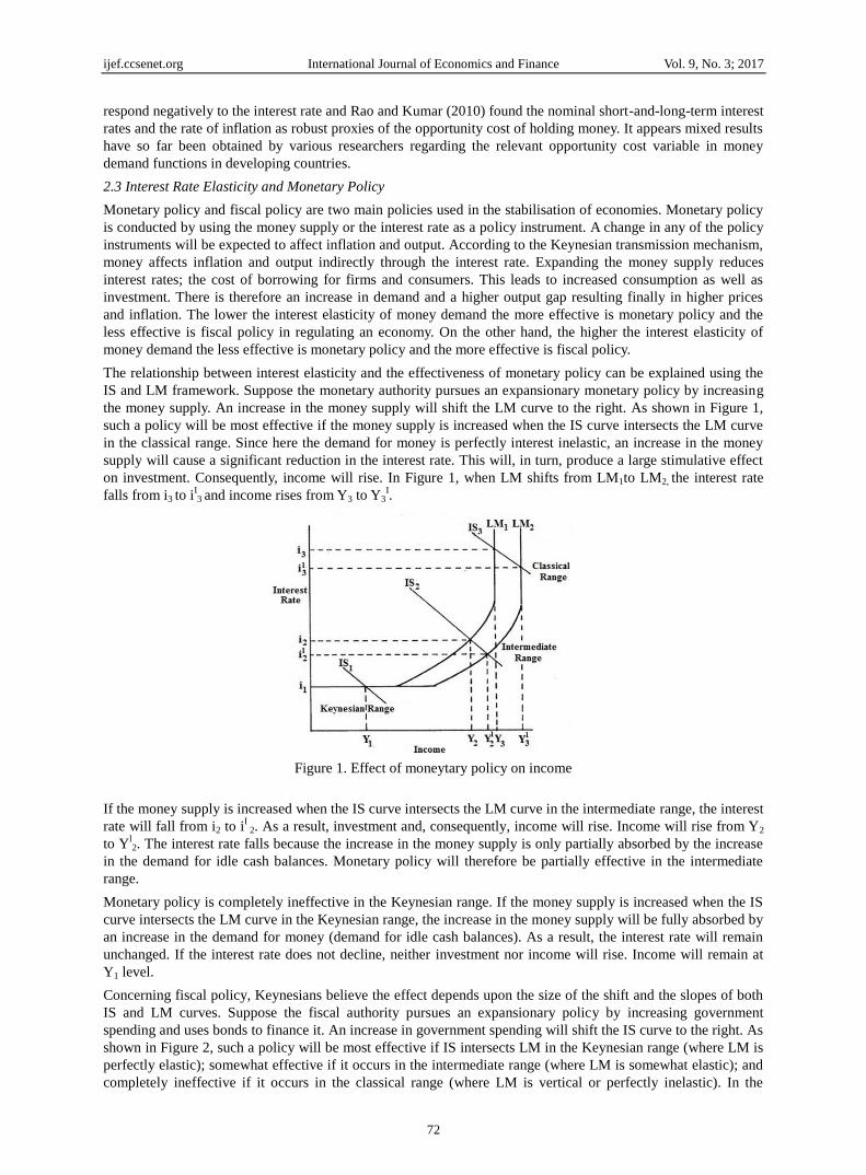
The relationship between interest elasticity and the effectiveness of monetary policy can be explained using the

IS and LM framework. Suppose the monetary authority pursues an expansionary monetary policy by increasing

the money supply. An increase in the money supply will shift the LM curve to the right. As shown in Figure 1,

such a policy will be most effective if the money supply is increased when the IS curve intersects the LM curve

in the classical range. Since here the demand for money is perfectly interest inelastic, an increase in the money

supply will cause a significant reduction in the interest rate. This will, in turn, produce a large stimulative effect

on investment. Consequently, income will rise. In Figure 1, when LM shifts from LM1to LM2, the interest rate

falls from i3 to iI3 and income rises from Y3 to Y3

I.

Figure 1. Effect of moneytary policy on income

If the money supply is increased when the IS curve intersects the LM curve in the intermediate range, the interest

rate will fall from i2 to iI

2. As a result, investment and, consequently, income will rise. Income will rise from Y2

to Yl2. The interest rate falls because the increase in the money supply is only partially absorbed by the increase

in the demand for idle cash balances. Monetary policy will therefore be partially effective in the intermediate

range.

Monetary policy is completely ineffective in the Keynesian range. If the money supply is increased when the IS

curve intersects the LM curve in the Keynesian range, the increase in the money supply will be fully absorbed by

an increase in the demand for money (demand for idle cash balances). As a result, the interest rate will remain

unchanged. If the interest rate does not decline, neither investment nor income will rise. Income will remain at

Y1 level.

Concerning fiscal policy, Keynesians believe the effect depends upon the size of the shift and the slopes of both

IS and LM curves. Suppose the fiscal authority pursues an expansionary policy by increasing government

spending and uses bonds to finance it. An increase in government spending will shift the IS curve to the right. As

shown in Figure 2, such a policy will be most effective if IS intersects LM in the Keynesian range (where LM is

perfectly elastic); somewhat effective if it occurs in the intermediate range (where LM is somewhat elastic); and

completely ineffective if it occurs in the classical range (where LM is vertical or perfectly inelastic). In the


73

Keynesian range, such an action will be most effective because the shift of IS from lS1 to ISl1 does not increase

the interest rate, thereby causing no adverse effect on private investment. However, in the classical range, similar

action causes such an increase in the interest rate that private investment equal to the increase in government

spending is crowded out. In the figure, when the shift occurs from IS3 to ISl3 the interest rate rises from i3 to i

l3.

But income stays at the same level, i.e., Y3. The interest rate rises because the increase in government spending

causes an increase in its borrowing from the market.

Figure 2. Effect of fiscal policy on income

In the case of the intermediate range, similar action is somewhat effective because only a part of its effect is

counterbalanced by a fall in private investment. In Figure 2, when a shift occurs from IS2 ISl2, the interest rate

rises from i2 to il2 and income, from Y2 to Y

l2. Thus, the effect of fiscal action depends, among other things, upon

the slope of the LM curve. The steeper the LM curve, the less will be its effect. Keynesians claim that there is

overwhelming evidence that the short run LM curve is not vertical: the demand for money is negatively related

to the interest rate.

To sum up, monetary policy is more potent in stabilising the economy when the demand for money is interest

inelastic, whilst fiscal policy will be a more effective tool when the demand for money is interest elastic.

3. Money Demand Models and Advantages of Panel Data

This section discusses the benefits to be derived from using panel data instead of pure time series or cross

sectional data. It also specifies the fixed effects and random effects models of the money demand function.

3.1 Advantages of Panel Data

Panel or longitudinal data set comprises time-series observations over cross-sectional units like countries, firms

and randomly-sampled individuals. It is either a balanced panel with the same time periods or unbalanced panel

with time dimension specific to each cross-sectional unit. Panel data sets have several benefits as compared to

pure time-series or cross-sectional data sets (Gujarati, 2003, pp. 638-640). Panel data ensures much larger data

which increases the degrees of freedom. There is more variability and less collinearity among the explanatory

variables which improve the efficiency of econometric estimates. It captures individual heterogeneity, that is

unobserved individual specific effects, leading to more reliable estimates. Panel data is good for uncovering

complex issues of dynamic behaviour. Economic behaviour is inherently dynamic. Koyck or Almon distributed

lag models involving current and lagged variables which are highly collinear are often used. The use of panel

data captures inter-individual differences which reduces the collinearity between the current and lagged variables.

Panel data sometimes simplifies statistical computation and inference. With non-stationary time series, the large

sample approximation distribution will not hold for the least squares and maximum likelihood estimators.

However, with independent observations across cross-sectional units one can invoke the Central Limit Theorem

and estimators will become asymptotically normal (Phillips & Moon, 1999, 2000; Quah, 1994). Panel data

analysis involves the use of fixed effects and random effects models which are discussed below.

3.2 The Fixed Effects Model

If money is regarded as one of several assets in a portfolio, a conventional demand for money function in


74

logarithmic form is specified as follows:

Inmt = β0 + β1InYt + β2InRt + β3InΠt + ԑ t (1)

where mt is real narrow money balances. Yt is the real GDP; Rt is the interest rate variable; пt is the inflation rate

variable; and the stochastic disturbance is εt. To avoid negatives the consumer price index is used as a proxy for

the inflation rate. Real money balances are assumed to be positively related to real income; that is, β1 is expected

to be positive. On the other hand, the interest rate (Rt) is expected to be negatively related to money demand so

that β2 carries a negative sign. Similarly, the expected inflation rate (πt) is anticipated to be negatively related to

money demand, so β3 is expected to be negative.

Pooling, or combining all the 120 observations for the eight African countries for the period 1980 to 2012, we

can rewrite the money demand function as:

Inmit = β0 + β1InYit + β2InRit + β3InΠit + ԑ it ; i = 1, 2, 3, 4, 5, 6, 7, 8 and t = 1, 2,…15 (2)

where i stands for the ith cross-sectional unit and t for the tth time period.

There are differences in the eight African countries in terms of socio-economic development. Estimating model

(2) without taking into account the individual country heterogeneity will lead to omitted variable bias. If the

country-specific effect is correlated with the independent variables a way to allow for the unobserved specific

effects of each country is to let the intercept vary for each country but still assume that the slope coefficients are

constant across nations. To see this, model (2) is written as:

Inmit = β0i + β1InYit + β2InRit + β3InΠit + ԑ it (3)

This is known as the fixed effects model. The subscript i is put on the intercept term to suggest that the intercepts

of the eight countries may be different. the differences may result from differences in characteristics of each

country, such as human development or degree of industrialization. Obviously the use of a fixed effects model

such as Equation (3) will lead to more accurate results as it takes into account individual country heterogeneity.

3.3 The Random Effects Model

If the country-specific effect is uncorrelated with the regressors a way of capturing individual heterogeneity is to

use the random effects model.

The basic idea is to start with (3):

Inmit = β0i + β1InYit + β2InRit + β3InΠit + ԑ it (3)

Instead of treating β0i as fixed, we assume that it is a random variable with a mean value of β0 (no subscript i

here). The intercept value for an individual country can be expressed as

Β0i = β0 + vi i = 1, 2, ... , N (4)

where vi is a random error term with a mean value of zero and variance of σv2.

Basically, the eight countries included in the sample are a drawing from a much larger universe of such countries.

The mean values of the intercept ( = β0) are the same for all the countries and the individual differences in the

intercept values of each country are reflected in the error term vi.

I substitute (4) into (3), to get:

Inmit = β0 + β1InYit + β2InRit + β3InΠit + vi + ԑ it

= β0 + β1InYit + β2InRit + β3InΠit + wit (5)

where wit = vi + εit

The composite error term wit consists of two components, vi, the cross-section error component, and εit, which is

the combined time series and cross-section error component. Equation (5) is the random effects model. Its

estimation, like the fixed effects model, will yield more reliable results. Thus, fixed and random effects error

correction models are used in the study.

4. Empirical Methods and Results

This section describes the empirical estimation methods and presents the results. This research work basically

involves the use of panel data to examine interest elasticity of demand for money in developing countries. The

research tools used consist of panel unit root tests, cointegration tests, error correction models with fixed and

random effects, and the panel Fully Modified Ordinary Least Squares (FMOLS) estimation technique. Panel unit

roots tests were carried out prior to cointegration analysis. Having established cointegration among the variables,

an error correction mechanism was used to capture the short run dynamics. Finally, the panel Fully Modified


75

Ordinary Least Squares method was used to estimate the long run money demand function. Money demand for

developing countries was found to be interest inelastic in the short run but interest elastic in the long run.

4.1 Empirical Tests and Estimation Methods

Before undertaking any regression analysis, the time series properties of the data are examined. There is the need

to ensure that all the variables are stationary in order to avoid the problem of spurious regression caused by

non-stationary variables. In doing so, I used the panel-based unit root tests developed by Levin, Lin, and Chu

(2002), Breitung (2000), Hadri (1999), and Im, Pesaran and Shin (2003). These researchers have shown that

panel unit root tests are more powerful than unit root tests applied to pure time series because the information in

the time series is augmented by that contained in the cross-section data. The computations of the test statistics

were done with EViews econometric software.

Having established that all the variables are integrated of the same order, I followed the methodology used by

Pedroni (1999) to test for cointegration. This method uses four panel statistics and three group panel statistics to

test the null hypothesis of no cointegration against the alternative hypothesis of cointegration. If the null

hypothesis is rejected in the case of the panel, then the variables of the money demand function are cointegrated

for all the countries. However, if the null hypothesis is rejected in the case of the group panel, then cointegration

exists among the relevant variables for at least one of the countries. Pedroni Residual Cointegration tests in cases

with no deterministic trend and with deterministic intercepts and trend were carried out with EViews.

Cointegration is established among the variables which means an error correction model can be run. This is a

representation of the short run demand for money. In this representation, short-run dynamics are captured by

estimating in first differences. Adjustments in reaction to the deviation of real money demand from the long-term

level are captured by including the equilibrium correction term. The error correction model was estimated for

both fixed and random effects with EViews. Finally, I used the panel fully modified OLS estimator (FMOLS) to

examine the long run money demand function because the Ordinary Least Squares (OLS) estimator is biased and

inconsistent when applied to cointegrated panels. Following Kao, Chiang, and Chen (1999) the estimations were

carried out in EViews.

4.2 Results

The panel data consists of eight African countries (N =1....8) for the period 1998 to 2012 (T =1.....15). The

selected countries are Angola (ANG), Equatorial Guinea (EQG), Gambia (GMB), Guinea-Bissau (GBS), Kenya

(KNY), Mali (MLI), Nigeria (NGR), Uganda (UGD). The data is extracted from World Bank Development

Indicators 2003. The data used are the logarithmic values of the variables concerned. The results of the panel unit

root tests under the H0 of Non-stationarity (Note: in the case of the Hadri test the null is that the variable is

stationary.) are displayed in Table 1.

Table 1. Panel unit root tests 1998-2012

Series LLC Breitung-t IPS-W ADF PP Hadri

In(m) -4.1589 0.38975 -0.2953 19.2893 27.2491 5.8906

(0.0000) (0.6516) (0.3839) (0.2539) (0.0388) (0.0000)

In(Y) -2.94841 -0.90186 -0.30913 16.4388 17.0316 6.04726

(0.0016) (0.1836) (0.3786) (0.4228) (0.3836) (0.0000)

In(R) -2.83391 0.59473 -0.45167 12.6099 12.8735 4.33513

(0.0023) (0.7240) (0.3258) (0.3980) (0.3783) (0.0000)

In(П) -4.76198 4.63555 -1.13218 24.8534 18.8992 6.47793

(0.0000) (1.0000) (0.1288) (0.0725) (0.2739) (0.0000)

∆In(m) -8.55875 -1.36149 -5.19219 53.4355 64.6709 5.9878

(0.0000) (0.0867) (0.0000) (0.0000) (0.0000) (0.0000)

∆In(Y) -4.41507 -2.85344 -3.19827 37.2922 63.2121 5.69993

(0.0000) (0.0022) (0.0007) (0.0019) (0.0000) (0.0000)

∆In(R) -5.85557 -2.27119 -3.00053 29.3306 48.3146 3.81265

(0.0000) (0.0116) (0.0013) (0.0035) (0.0000) (0.0001)

∆In(П) -6.22078 -2.09465 -3.94871 44.9151 54.0124 5.88945

(0.0000) (0.0181) (0.0000) (0.0001) (0.0000) (0.0000)

Note. The tests are: Levin, Lin and Chu (2002, LLC), Breitung (2000), Im, Pesaran and Shin (2003, IPS), ADF Fisher (ADF), PP Fisher (PP),

and Hadri (1999). The probability values are reported in parentheses.


76

These tests give somewhat mixed results. With the exception of the LLC and PP tests all the other tests confirm

that In(m) is non-stationary and all the other tests apart from the LLC test indicate that In(Y) is non-stationary at

the 5% level of significance. Also, all tests apart from the LLC test confirm that In(R) and In(П) are

non-stationary at the 5% level of significance. Most of the tests indicate that the first differences of these

variables are stationary and so one can conclude that the variables are I(1) in their levels.

Tables 2 and 3 show results for Pedroni Residual Cointegration between the three variables in equation (1) in

cases with no deterministic trend and with deterministic intercepts and trend under the H0 of No cointegration.

The majority of the reported tests show that there is cointegration between these variables at the 5% level.

Table 2. Pedroni residual cointegration tests

No deterministic trend

Test Statistics Statistics Weighted Statistics

Panel v-Statistic -0.43828 -0.51533

(0.6694) (0.6968)

Panel rho-Statistic 0.317002 0.202557

(0.6244) (0.5803)

Panel PP-Statistic -3.19433 -3.29877

(0.0007) (0.0005)

Panel ADF-Statistic -2.73709 -3.81356

(0.0031) (0.0001)

Group rho-Statistic 1.262764

(0.8967)

Group PP-Statistic

-4.41861

(0.0000)

Group ADF-Statistic

-3.94513

(0.0000)

Note. The probability values are reported in parenthesis.

Table 3. Pedroni residual cointegration tests

Deterministic intercepts and trend

Test Statistics Statistics Weighted Statistics

Panel v-Statistic -1.73902 -1.82341

(0.9590) (0.9659)

Panel rho-Statistic 1.026154 1.319513

(0.8476) (0.9065)

Panel PP-Statistic -5.01552 -3.68232

(0.0000) (0.0001)

Panel ADF-Statistic -2.69266 -2.05317

(0.0035) (0.0200)

Group rho-Statistic 2.261932

(0.9881)

Group PP-Statistic

-4.89011

(0.0000)

Group ADF-Statistic

-3.17671

(0.0007)

Note. The probability values are reported in parenthesis.

Tables 4 and 5 give the estimated error correction model parameters, with the fixed and random effects

respectively. These can be interpreted as the short run money demand functions. Changes in the interest rate is

insignificant while changes in the expected rate of inflation is significant in both the fixed and random effects

models at the 5% level. It means the interest rate does not influence significantly the demand for money while

the expected rate of inflation exerts a significant influence on money demand in the short run. The error

correction term in the fixed effect model is statistically significant and negative. It indicates that agents adjust to

equilibrium at the rate of 24% annually. The error correction term in the random effects model is also negative


77

but insignificant with a speed of adjustment of 0.04% annually.

Table 4. Error correction model for the money demand with fixed effects

Variables Coefficient Std. Errors t-Statistics Prob.

∆In(mt-1) -0.06403 0.089062 -0.71894 0.4747

∆In(Yt-1) 0.278095 0.279528 0.994875 0.3234

∆In(Rt-1) 0.056971 0.071929 0.79204 0.4311

∆In(Пt-1) -0.51387 0.189617 -2.710048 0.0085

Ut-1 -0.24201 0.062592 -3.866464 0.0003

Constant 0.342991 0.060088 5.70817 0.0000

R-squared 0.650218 Mean dependent var 0.05701

Adjusted R-squared 0.598012 S.D. dependent var 0.277258

S.E. of regression 0.175789 Akaike info criterion -0.50903

Sum squared resid 2.070412 Schwarz criterion -17668

Log likelihood 30.85227 Hannan-Quinn criter. -0.37598

F-statistic 12.45481 Durbbin-Watson stat 1.814502

Prob(F-statistic) 0.0000

Table 5. Error correction model for the money demand with random effects


∆In(mt-1) 0.029066 0.084701 0.343159 0.7325

∆In(Yt-1) 0.723468 0.257487 2.809723 0.0064

∆In(Rt-1) -0.00626 0.070116 -0.0893 0.9291

∆In(Пt-1) -0.71288 0.12692 -5.61678 0.0000

Ut-1 -0.00044 0.000911 -0.48628 0.6282

Constant 0.106548 0.031227 3.412036 0.0011

R-squared 0.528121 Mean dependent var 0.05701

Adjusted R-squared 0.495351 S.D. dependent var 0.277258

S.E. of regression 0.196961 Sum squared resid 2.793128

F-statistic 16.11627 Durbin-Watson stat 2.000083

Prob(F-statistic) 0.0000

Equation (1) estimates based on the Fully Modified Ordinary Least Squares (FMOLS) are presented in Table 6.

The income elasticity is significant at the 5% level and greater than unity. Both the rate of interest and the

expected rate of inflation have negative signs, but while the interest rate is significant the expected rate of

inflation is insignificant at the 5% level. This indicates that whilst the interest plays a significant role in

determining the demand for money in developing countries the expected rate of inflation does not.

Table 6. Panel Fully Modified Least Squares (FMOLS) for the money demand


In(Yt) 2.47326 0.357701 6.914324 0.0000

In(Rt) -0.319097 0.122697 -2.600682 0.0113

In(Пt) -0.444922 0.261601 -1.700769 0.0930

R-squared -138.245418 Mean dependent var 16.2074

Adjusted R-squared -210.729334 S.D. dependent var 1.712992

S.E. of regression 24.92561 Sum squared resid 45353.88

Long-run variance 0.02415

5. Conclusion

In the light of the controversy surrounding the role of the interest rate in money demand functions of developing

countries, this study set out to investigate the interest elasticity of the money demand function in developing

countries using panel data of eight African countries for the period 1998 to 2012.


78

A review of the theoretical literature indicates that Fisher’s postulation of the quantity theory was the earliest

attempt to formulate a money demand theory. Fisher assumes money is held for only transaction purposes. With

money market equilibrium, the supply of money is equal to the demand for money, and the equation can be

transformed into a money demand function where the amount of cash balances held is purely a function of

nominal income. According to Keynes, the interest rate, which influences money demand appreciably, and real

income determine the demand for real cash balances. To further develop the Keynesian theory, Baumol (1952)

and Tobin (1956) show that the transactions demand for money is also sensitive to the interest rate. Since real

assets are considered a form of holding wealth the expected rate of inflation relative to the expected return on

money is introduced as a variable in the money demand function.

Empirical evidence from developing countries to support the theory of money demand provides mixed results.

For instance, Kumar, Webber, and Fargher (2010) estimated the demand for real narrow money (M1) for Nigeria

over the period 1960-2008.They found the interest rate elasticity to be negative and significant whilst Dagher and

Kovanen (2011) in a study of the demand for money for Ghana found the interest rate to be statistically

insignificant.

The relationship between interest elasticity and the effectiveness of monetary policy is explained using the IS and

LM framework. It is found that monetary policy is more potent in stabilising the economy when the demand for

money is interest inelastic, whilst fiscal policy will be a more effective tool when the demand for money is

interest elastic.

Panel data is used in the study as it has several benefits as compared to pure time-series or cross-sectional data

sets. First, the study tests the panel variables for unit roots and shows that they exhibit a unit root. Pedroni

cointegration tests provide evidence of cointegration among the variables. This gives strong evidence that the

variables have long run equilibrium. The Fully Modified Ordinary Least Squares procedure developed by

Pedroni is used to produce consistent estimates of the relevant panel variables in the cointegrated money demand

function. Estimates for the entire sample period of 1998 to 2012 show that the demand for money responds

negatively to variations in the interest rate and the expected rate of inflation in the long run. The interest rate

proves to be statistically significant in the long run; the expected rate of inflation on the other hand is statistically

insignificant in the long run.

The error correction models which represent the short run money demand function show that the interest rate is

insignificant while the expected rate of inflation is statistically significant. This confirms the claim by some

economists that the interest rate does not exert a significant influence on money demand as far as developing

countries are concerned. The study shows that in the short run when substitutability between money and

financial assets is limited, the appropriate opportunity cost variable in the money demand function is the

expected rate of inflation. Although these findings differ from those of some other researchers, they can be

explained by the fact that, with financial innovation in the long run, economic agents are likely to get access to

more financial assets. This increases the substitution between money and financial assets and the interest rate

becomes the appropriate opportunity cost variable in the money demand function for developing countries.

In conclusion, the demand for money should be regarded as being interest inelastic in the short run but interest

elastic in the long run in developing economies. The study employs panel data techniques, with more efficient

econometric estimates, and therefore contributes immensely to the theoretical literature of the demand for money

in developing countries. An important policy implication that can be inferred from the results of this study is that

fiscal policy rather than monetary policy should be utilised to stabilise the economies of developing countries.

With money demand serving as an important aid to policy formulation, the study recommends continued

research in money demand especially regarding issues of stability and volatility of money demand functions in

developing countries.

References

Abdulkheir, A. Y. (2013). An Analytical Study of the Demand for Money in Saudi Arabia. International Journal

of Economics and Finance, 5(4). https://doi.org/10.5539/ijef.v5n4p31

Abdullah, H., Ali, J., & Matahir, H. (2010, July). Re-Examining the Demand for Money in Asean-5 Countries.

Asian Social Science, 6(7). https://doi.org/10.5539/ass.v6n7p146

Arestis, & Demetriades, P. O. (1991, September). Cointegration, Error Correction and the Demand for Money in

Cyprus. Applied Economics, 23(9), 1417-24. https://doi.org/10.1080/00036849100000192

Arize, A. C., & Nam, K. (2012). The Demand for Money in Asia: Some Further Evidence. International Journal

of Economics and Finance, 4(8). https://doi.org/10.5539/ijef.v4n8p59


79

Baharumshah, A. Z., Mohd, S. H., & Masih, A. M. M. (2009). The Stability of Money Demand in China:

Evidence from ARDL Model. Economic Systems, 33(3), 231-244.

https://doi.org/10.1016/j.ecosys.2009.06.001

Bahmani, S. (2013). Exchange rate volatility and demand for money in less developed countries. Journal of

Economics & Finance, 37, 442-452. https://doi.org/10.1007/s12197-011-9190-y

Bahmani-Oskooee, M., & Bahmani, S. (2015). Nonlinear ARDL Approach and the Demand for Money in Iran.

Economics Bulletin, 35(1), 381-391.

Baumol, W. J. (1952). The Transactions Demand for Cash: An Inventory Theoretic Approach. Quarterly Journal

of Economics, 66, 545-556. http://dx.doi.org/10.2307/1882104

Breitung, J. (2000). The Local Power of some Unit Root Tests for Panel Data. In B. Baltagi (Ed.), Advances in

Econometrics: Non-stationary Panels, Panel Cointegration, and Dynamic Panels (pp. 161-178).

Amsterdam, JAI Press. https://doi.org/10.1016/S0731-9053(00)15006-6

Carrera, C. (2008). Long-run Money Demand in Latin-American Countries: Nonestationary Panel Data

Approach. Retrieved from http://www.williams.edu/cde/

Dagher, J. C., & Kovanen, A. (2011, November). On the Stability of Money Demand in Ghana: A Bounds

Testing Approach. IMF Working Paper No. 11/273.

Fisher, I. (1911). The Purchasing Power of Money (New York; Macmillan, 1911). PMCid: PMC2332238

Friedman, M. (1956). The Quantity Theory of Money: A Restatement. Studies in the Quantity Theory of Money,

University of Chicago Press.

Gujarati, D. N. (2003). Basic Econometrics (4th ed.). Boston: McGraw Hill-Publishing.

Hadri, K. (1999). Testing the Null Hypothesis of Stationarity Against the Alternative of a Unit Root in Panel

Data with Serially Correlated Errors. Manuscript, Department of Economics and Accounting, University of

Liverpool.

Hamori, S. (2008). Empirical Analysis of the Money Demand Function in Sub-Saharan Africa. Economics

Bulletin, 15, 1-15.

Harb, N. (2004). Money Demand Function: A Heterogeneous Panel Application. Applied Economics Letters, 11,

551-555. https://doi.org/10.1080/1350485042000225739

Herve, D. B. G., & Shen, Y. (2011). The Demand for Money in Cote d'Ivoire: Evidence from the Cointegration

Test. International Journal of Economics and Finance, 3(1).

Hossain, A. (2006). The Income and Interest Rate Elasticities of Demand for Money in Bangladesh: 1973-2003.

The ICFAI Journal of Monetary Economics, 73-96.

Im K. S., Pesaran, M.H., & Shin, Y. (2003). Testing for Unit Roots in Heterogeneous Panels. Journal of

Econometrics, 115, 53-74. https://doi.org/10.1016/S0304-4076(03)00092-7

Kao, C., Chiang, M., & Chen, B. (1999). International R&D Spillovers: An Application of Estimation and

Inference in Panel Cointegration. Oxford Bulletin of Economics and Statistics, 61(4), 691-709.

https://doi.org/10.1111/1468-0084.61.s1.16

Keynes, J. M. (1936). The General Theory of Employment, Interest and Money. 7. JMK. (1936) London:

Macmillan.

Kumar, S., Chowdhury, M., & Rao, B. B. (2010). Demand for Money in the Selected OECD Countries: A Time

Series Panel Data Approach and Structural Breaks. MPRA Paper No. 22204.

Kumar, S., Webber, D. J., & Fargher, S. (2010, September). Money Demand Stability: A Case Study of Nigeria.

Auckland University of Technology.

Laidler, D. E. W. (1985). The Demand for Money: Theories and Evidence (3rd ed.). New York: Dunn-Donnelley.

PMCid:PMC499270.

Levin, A., & Lin, C. F. (1993). Unit Root Tests in Panel Data: New Results. University of California, San Diego,

Discussion Paper, No. 93-56.

Levin, A., Lin, C. F., & Chu, C. J. S. (2002). Unit Root Tests in Panel Data: Asymptotic and Finite-Sample

Properties. Journal of Econometrics, 108, 1-24. https://doi.org/10.1016/S0304-4076(01)00098-7

Marshall, A. (1923). Money, Credit and Commerce. London: Macmillan.


80

Narayan, P. K., Narayan, S., & Mishra, V. (2009). Estimating Money Demand Functions for South Asian

countries. Empirical Economics, 36(3), 685-696. https://doi.org/10.1007/s00181-008-0219-9

Pathak, D. S. (1981). Demand for Money in a Developing Country: An Econometric Study. Indian Economic

Journal, 29, 10-16.

Pedroni, P. (1999). Critical Values for Cointegration Tests in Heterogeneous Panels with Multiple Regressors.

Oxford Bulletin of Economics and Statistics, 61, 653-670. https://doi.org/10.1111/1468-0084.61.s1.14

Phillips, P. C. B., & Moon, H. R. (1999). Linear Regression Limit Theory for Nonstationary Panel Data.

Econometrica, 67, 1057-1111. https://doi.org/10.1111/1468-0262.00070

Phillips, P. C. B., & Moon, H. R. (2000). Nonstationary Panel Data Analysis: An Overview of some Recent

Development. Econometric Reviews, 19, 263-286. https://doi.org/10.1080/07474930008800473

Pigou, A. C. (1917, November). The Value of Money. The Quarterly Journal of Economics, 37, 38-65.

https://doi.org/10.2307/1885078

Rao, B. B., & Kumar, S. (2007, November). Cointegration, Structural Breaks and the Demand for Money in

Bangladesh. MPRA Paper No. 1546.

Rao, B. B., & Kumar, S. (2009). A Panel Data Approach to the Demand for Money and the Effects of Financial

Reforms in the Asian Countries. Economic Modelling, Elsevier.

https://doi.org/10.1016/j.econmod.2009.03.008

Rao, B. B., & Kumar, S. (2010). Error-Correction Based Panel Estimates of the Demand for Money of Selected

Asian Countries with the Extreme Bounds Analysis. MPRA Paper No. 27263.

Rao, B. B., & Singh R. (2005). Demand for money in India: 1953-2003. Applied Economics, 38, 1319-1326.

Sichei, M. M., & Kamau, A. W. (2012). Demand for Money: Implications for the Conduct of Monetary Policy in

Kenya. International Journal of Economics and Finance, 4(8). https://doi.org/10.5539/ijef.v4n8p72

Simmons, R. (1992). An Error-correction Approach to Demand for Money in Five African Developing Countries.

Journal of Economic Studies, 19(1), 29-47. https://doi.org/10.1108/01443589210015935

Singh, R., & Kumar, S. (2012). Application Of The Alternative Techniques to Estimate Demand for Money in

Developing Countries. The Journal of Developing Areas, 46(2), 43-63.

https://doi.org/10.1353/jda.2012.0036

Suliman, S. Z., & Dafaalla, H. A. (2011). An econometric analysis of money demand function in Sudan, 1960 to

2010. Journal of Economics and International Finance, 3(16), 793-800. https://doi.org/10.5897/JEIF11.122

Tang, C. F. (2009). How Stable is the Demand for Money in Malaysia? New Empirical Evidence from Rolling

Regression. IUP Journal of Monetary Economics.

Terriba, O. (1973). The Demand for Money in Nigeria. Economic Bulletin of Ghana, 3, 14-22.

Tobin, J. (1956). The Interest Elasticity of Transactions Demand for Cash. The Review of Economics and

Statistics, 38, 241-47. https://doi.org/10.2307/1925776

Tobin, J. (1958). Liquidity Preference as Behaviour Towards Risk. The Review of Economics Studies, 25(67),

65-86. https://doi.org/10.2307/2296205

Valadkhani, A. (2008). Long and Short Run Determinants of the Demand for Money in the Asian-Pacific

Countries: An Empirical Panel Investigation. Annals of Economics and Finance, 9, 77-90.

Wong, C. H. (1977). Demand for Money in Developing Countries: Some Theoretical and Empirical Results.

Journal of Monetary Economics, 3(1), 59-86. https://doi.org/10.1016/0304-3932(77)90005-8

Copyrights

Copyright for this article is retained by the author(s), with first publication rights granted to the journal.

This is an open-access article distributed under the terms and conditions of the Creative Commons Attribution

license (http://creativecommons.org/licenses/by/4.0/).

Documents

An Investigation into the Interest Elasticity of Demand