An Introduction to Using Simulink

COURSE NOTES

Eric Peasley, Department of Engineering Science, University of Oxford Adapted and updated by Dr I. F. Mear using MATLAB 2017b and MATLAB 2018b

version 5.0, 2018

1

Table of Contents

Introduction ......................................................................................................................................... 2

What is Simulink? ................................................................................................................................ 3

Working with Blocks ............................................................................................................................ 4

Block Settings ....................................................................................................................................... 5

Model Annotation ................................................................................................................................ 6

The Solver ............................................................................................................................................ 7

Sources Library ..................................................................................................................................... 8

Sinks Library ......................................................................................................................................... 9

Math Operations Library .................................................................................................................... 10

User Defined Functions & Lookup Tables .......................................................................................... 11

Ports & Subsystems............................................................................................................................ 12

Signal Routing & Logicals ................................................................................................................... 14

Integration and Differentiation .......................................................................................................... 16

MATLAB & Simulink Working Together .............................................................................................. 17

Examples Models ............................................................................................................................... 18

Simulink Shortcuts ............................................................................................................................. 25

The Solver: Zero-Crossing Options ..................................................................................................... 27

Simulink Online Documentation ........................................................................................................ 28

Further Examples ............................................................................................................................... 29

Oxford University MATLAB Installation .............................................................................................. 30

2

Introduction

This document is part of the “Introduction to Using Simulink” seminar. This seminar is designed for people that have never used Simulink. There are two components to the seminar. There are exercises in a separate document that will take you step by step through the tasks required to build and use a Simulink model. Once you get started using Simulink, you will find a lot of the functionality is self-intuitive. Inevitably, there are things that need a bit more explanation. So the other part of the Seminar is a talk and demonstration. This document contains the notes for the talk. It would be impossible to put everything about Simulink into such a short document, so this document concentrates on the parts of the package that are considered the most useful. It also aims to highlight features that are not obvious to the casual user. The intention is that you use these notes as a reference when carrying out the exercises and when building your own models. Although these notes have their limits, I hope that they should be sufficient to get you started using the package and that they cover most of your modelling needs. This is not a Simulink manual. Sooner or later you will need to know more detail about something within Simulink. This document is intended to be used in conjunction to the documentation available within the package. Mathworks, creators of MATLAB & Simulink, provide extensive online documentation for Simulink that can be accessed using the MATLAB help system. There is so much online documentation that not many people have the time or inclination to read all of it. So an aim of the Seminar is to emphasize the things that you ought to know about Simulink and to give you some idea about where you can find any other information that you require.

3

What is Simulink?

Simulink is a visual programming interface designed to make modelling systems intuitive. It offers a way to solve equations numerically using a graphical user interface, rather than requiring code. Models contain blocks, signals and annotation on a background:.

Blocks are mathematical functions, they can have varying numbers of inputs and outputs.

Signals are lines connecting blocks, transferring values between them. Signals are different data

types, for example numbers, vectors or matrices. Signals can be labelled.

Annotations of text or images can be added to the model, and while not used in the calculations they can make it easier for others to understand design decisions in the model.

The Simulink Toolbar

Above the main canvas of a Simulink model, is the toolbar.

Text Annotation Blocks

Signal and Label

Run Model To run the simulation, press the green arrow. Be aware there are different modes e.g. ‘Normal’. If you are working with hardware

the mode will be ‘External’.

The textbox is how many seconds you want the simulation

to run for.

Model Settings

All of the settings related to how to numerically solve the equations of the model

are found in “Model Configuration Parameters”

Cog.

Build Model If your model is interacting with hardware, you will need to build the model before it can run. The current status is shown in the lower left of the Simulink window.

4

Working with Blocks

Adding Blocks to Model There are two ways to add blocks to a model: the Library Browser or the Quick Search:

Library Browser

Shows all blocks available in Simulink, sorted by folders such as ‘Math

Operations’ or ‘Signal Routing’. There is a search bar on the top left. Drag

blocks from the library straight onto your model canvas.

Quick Search

Directly search for blocks by single clicking on the background of your

model and typing in a search term. Select a block from the search results to

quickly add it to your model.

Automatic Block Input Box When adding a block to a model for the first time, the most common

parameter will often pop up automatically for a value to be specified.

e.g. If you add a Gain Block it will ask you to specify the gain value.

Interacting with this can save time opening the Block Parameters menu

Positioning Blocks Blocks can be moved by simply clicking and dragging.

Connect blocks by clicking output of one block and dragging it to an input of another block.

Once a signal connects two blocks, it can be clicked and dragged to be repositioned.

To create a branch from an existing signal, hold ctrl while clicking and dragging.

Blocks can be rotated/flipped for better positioning: Right click block, select “Rotate & Flip”.

Overview of Libraries

Library Name Type of Blocks Examples of Blocks

Sources Provide inputs to your model Constant, Sine Wave, Step

Sinks Provide ways to view or export data Scope, XY Graph, To Workspace

Math Operations

Common mathematical functions to apply to data.

Add, Divide, Abs

Ports & Subsystems

Create different subsystems (resettable, triggered etc)

Subsystem, Enable port, Inputs and Outputs: In1 and Out1

User Defined Functions

Implement custom functions Fcn, MATLAB Fcn

Lookup Tables Use functions defined as discrete data 1-D Lookup Table

Signal Routing Organise signals from blocks Mux, BusCreator, Goto, Switch

Continuous Systems with continuous states Integrator, Derivative

Discrete Systems with discrete states Unit Delay, Discrete Derivative

Logical and Bit Operations

Boolean operators for comparisons Compare To Zero, Logical Operator

5

Block Settings Each block has its own settings in Block Parameters and Block Properties.

Block Parameters Double click on a block to open Block Parameters, where you change the settings for that specific block. e.g. In a Saturation Block, you can set the upper and lower limit.

Block Properties Right click and select “Properties…” to open the Block Properties. This contains settings to do with how the block works as part of the larger model.

You can change what information is displayed about the block in the Block Annotation tab. For properties to be displayed under a block in your model, move properties from the left to the right by using the double arrow (>>). You can also add your own text around the various %< Properties> %<BlockType> x0 = %<InitialCondition> m

The example above shows how to display the block type and initial condition to under an Integration Block.

Simulink Models & MATLAB Variables Simulink blocks can contain MATLAB variables. These variables need to be defined in the MATLAB workspace before you run the Simulink model, otherwise an error will state there is an undefined function or variable. Below c and zeta, in the gain block, are defined in the MATLAB workspace.

It is good practice to design a MATLAB script that sets up all the parameters needed in your model. It is easier to change a variable in a script than to open many block parameter menus in Simulink.

It allows you to set up loops to run a simulation for many values of c for example (see page 17).

6

Model Annotation Text and Image Annotation You can double click anywhere on the background of your model and type a comment. Pressing Enter will select the “Create Annotation” option of the quick menu. You can also use the shortcuts on the left to bring up the annotation tool. There are many formatting options. You can insert Text and images

Greek letters: use backslash (e.g. \alpha for 𝛼).

TeX typesetting: Right click text box, select Properties… and tick Enable TeX Commands.

Signal Labelling The lines connected the blocks are called signals. By double-clicking directly on a signal you can label it. This makes it easier to recall what the signals are, gives useful legend labels on scopes and can be used when importing data into MATLAB (see page 17).

Display Menu – Useful for Debugging Errors The Display Menu allows you to easily toggle on and off information about your signals.

Display > Signals & Ports > Port Data Types Shows you the data type on each signal e.g. double or logical

Display > Signals & Ports > Signal Dimensions Shows you the dimensions of each signal e.g. [3 4] vector

Useful if you have a dimension mismatch error.

Display > Sample Time > All

Colours each block to show the different sample times, this is particularly useful when you obtain a sample time mismatch error.

Display > Signals & Ports > Wide Non-scalar Lines Gives different thicknesses to each signal that is actually a combination of signals. Useful if you have a dimension mismatch error. This visualises Mux and Bus signals (see page 14).

Format Menu – Block Annotation By right-clicking on any block, you can select the Format menu to:

Show/Hide Block Name

Add foreground and background colours

Add shadows to blocks

7

The Solver

Most of the time, you can just use the default settings to run your model. However you will

sometimes find that you will want the model to use smaller steps, or fixed width steps. This is all

configurable on the Solver page of the Configuration Parameters.

From the menu bar on your model select Simulation ► Model Configuration Parameters

Or simply use the shortcut on the toolbar

Once opened, select Solver.

There are many configurable

settings.

Start/Stop time: It is suggested that you leave the start time as zero.

The stop time is same as in the toolbar at the top of your model.

There are two types of solver:

o A variable step solver (the default): This will automatically adjust the step size as the

model runs. If you are using variable step generally keep the default solver (ode45).

Set the Max step size to a small fixed value to improve the smoothness of any plots.

o A fixed step solver will be necessary for models with discrete components. If it also

has no continuous components, change the solver to Discrete (no continuous states)

and set the step size to a known value. The fixed solvers are numbered in order of

simplicity, ode1 being the simplest.

Zero-crossing options: Under “Additional Parameters” you will find the Zero-crossing

options. Further details about zero-crossing are found on page 27.

For more information about solvers, click on the Help button at the bottom of the configuration

parameters window, while you are viewing the solver section.

8

Sources Library Source blocks provide different signals for your model.

The simplest source is simply a Constant. A block that outputs a constant value. The Signal Builder allows custom signals to be built using a graphical user interface (see right).

For more typical periodic functions, see the table below with key blocks from this library:

Block Key Block Parameters Block Key Block Parameters

Amplitude and Frequency

Bias and Phase

Time can be input as external signal

Amplitude

Period (seconds)

Pulse Width (% of period)

Phase Delay (seconds)

Step Time

Initial Value

Final Value

Waveform: Sine, Square,

Sawtooth or Random

Amplitude

Frequency

Units (rad/sec or Hertz)

Assume we want to use the sine wave block to look at the frequency response of a system. Repeatedly editing the block parameters to change the frequency of the sine wave is tedious. The alternative is to use an external time input to the block.

To do this, in the Sine Wave block parameters you set the Time parameter to Use external signal and set the frequency to 2*pi. You then connect a clock to the new input via a slider gain. The slider then sets the frequency of the sine wave.

9

Sinks Library The blocks in this library are mostly used for viewing data from the model.

Scope

Scope plots inputs against time. It has an extensive toolbar.

The magnifying glass icon allows you to zoom in and out in the 𝑥 and 𝑦 direction simultaneously and individually. The hand allows you to pan or drag the plot around.

The scaling icons allow you to automatically scale axes individually or simultaneously in the 𝑥 and 𝑦 directions.

The Cog icon opens a Configuration Menu. This allows you to set the:

number of input ports

layout of the plots

ranges of the axes

legend

enable data logging (see below)

The Logging Tab contains a tick box to ‘Log data to workspace’. If this is enabled then whenever the simulation is run, a variable is automatically populated in the MATLAB workspace. You can name the variable and set the datatype.

Data Logging without Scope: To Workspace Block Data can also be sent to the MATLAB workspace using a To Workspace block. Any input to the block is sent to the MATLAB workspace after the model has been run. The variable name by default is ‘simout’ but can be changed along with data type. See page 17 for more details.

Other Blocks in the Sinks Library

Displays values in a textbox while the simulation is running.

Plots the top input X against lower input Y in a figure within Simulink. Cannot easily change the axis labels or titles, so it is better to use the To Workspace block to send data to MATLAB, then plot there.

Halts the simulation

10

Math Operations Library The blocks in this library relate to common mathematical functions.

Add, Subtract and Sum Blocks The Add, Subtract and Sum blocks are all essentially the same. By

changing the Icon shape and List of signs in the block parameter you

can convert one into the other (see right).

Product and Divide Blocks The Product and Divide blocks are also interchangeable. You can use a list of asterisks

and forward slashes in the number of inputs block parameter to define operations

needed e.g. Block to the right was created by number of inputs = /*/**

Gain Block The Gain block can be used to multiply a signal by a constant value. You must configure the Block Parameters to perform matrix or element-wise (array) multiplication.

Array and Matrix Multiplication:

Array multiplication with column vector 𝐾 = [12

] and Matrix multiplication where 𝐾 = [5 67 8

]

Both examples have Gain block configured to do Matrix(u*K) multiplication. For a Gain block to

contain a matrix or vector, simply use MATLAB notation. For example [5 67 8

] is entered as

[5, 6; 7, 8] – commas separate row elements and semi colons separate columns.

Mathematical Functions There are lots of blocks for specific mathematical functions:

The Abs block finds the magnitude or absolute value of a signal, the Unary Minus block negates a signal and the Bias block adds a constant to a signal. The Sign block outputs +/- 1 depending on the sign of the input.

There are also blocks with multiple functions to choose from: The Math Function block can perform many different functions: square, square root, log, reciprocal etc. A block parameter allows you to select which particular function you want. The Trigonometric Function block operates in a similar manner but for cos, sin, tan-1 etc.

11

User Defined Functions & Lookup Tables

User Defined Functions Sometimes you cannot find the exact function that you want. If this is the case, then try the block called Fcn. This allows you to enter a mathematical expression using a restricted set of operators and functions:

To see what is allowed, click on the Help in the block parameters. If you need something a bit more complicated then you can write your own MATLAB function and use the block MATLAB Fcn:

This block has been configured to call the MATLAB function myabs, shown left. x is the input and y is the output. Notice that the MATLAB function is not stored as a .m file in the working directory, instead you are editing code stored within the block itself. This can be seen from Block: MyModel/MATLAB Function.

If you are using Simulink to create a program using the Real Time Workshop, then you will need to use the Embedded Matlab Function or an S Function. S functions are used to embedded Matlab, C or Fortran into your model.

Look Up Tables If all else fails, then you can use a look up table to define your function.

You need two vectors to do this. A vector of input values and a vector containing the table of corresponding output values. You enter these in to the appropriate block parameter. For intermediate values, the output is calculated using interpolation. Extrapolation is used to calculate values beyond the specified input range. There are a range of look up tables to suit different needs (e.g. 1-D Lookup Table, 2-D Lookup Table), see the documentation for further details.

12

Ports & Subsystems A subsystems is a collection of blocks grouped together to carry out a particular task. They help to keep models organised and easier to understand. The example subsystem on right takes two inputs. It doubles the first input, quadruples the second input and outputs the sum.

Creating a Subsystem Drag in a Subsystem block from the Ports and Subsystems library

OR

Select the blocks that you want to put into a subsystems and right click then select Create Subsystem from Selection in the menu that appears.

You can have many nested subsystem (i.e. a subsystem in a subsystem).

Once you have a subsystem, you can open it by double clicking the block. This opens a new tab

showing the blocks of the subsystem. Exit the subsystem and return to the top page by:

Selecting the ‘Up to Parent’ arrow

OR

Selecting the home tab, e.g. ‘MyModel’

Input and output ports are called In and Out. If you need extra input/output ports, they can be found in the Ports and Subsystems library or the relevant Source / Sink library.

Trigger, Reset and Enable Inputs to Subsystems

You may need a part of your model to only occur when an appropriate signal is applied, or for blocks to reset at certain time intervals. For this you place an Enable, Trigger or Reset block inside the subsystem. These will create an appropriate input port on the subsystem.

There is extensive documentation on the MathWorks website giving comparisons of each of these subsystems. A summary is given below:

Enabled Subsystems: Subsystem only runs when signal is 1 through the enable input, a 0 will disable it. The block parameters of the output ports allow configuration to either hold the current value or reset to a specified value when the subsystem is disabled. Triggered Subsystems: Executes one step each time the appropriate signal is applied to the trigger input. You can configure the trigger input to react to a rising edge, a falling edge or both edges. Resettable Subsystems: Executes at every time step but conditionally resets the states of blocks within it to their initial conditions when a trigger event occurs at the reset port.

13

Masked Subsystems A mask is special type of subsystem. It offers a custom interface for a subsystem and hides the content, making it appear as a built in ‘base’ block with its own icon and custom parameter dialog box. It simplifies the graphical appearance of a model and controls access to the block content. Consider an example subsystem below which simply produces a straight line 𝑦 = 𝑚𝑥 + 𝑐 where 𝑥 is the simulation time steps and 𝑚 and 𝑐 are defined by Gain and Constant blocks respectively. To edit 𝑚 and 𝑐 you would normally have to open the subsystem, and interact with each of the block parameters (this involved multiple windows and clicks).

If we instead turn this subsystem into a mask (right click -> Mask -> Create Mask) then we could create a custom dialog block. Whenever we click on this new masked susbsytem, we would get one dialog box where we can conveniently set 𝑚 and 𝑐. For information on creating your own masks, see this video: https://uk.mathworks.com/videos/creating-a-mask--masking-fundamentals-1480968643715.html

Program Control: For, While, If and Case

Within the Ports and Subsystems library, you will see subsystems that perform the Simulink equivalent of For and While loops and If and Case statements. The For and While loops will perform a number of loops for each step of the simulation. They each contain a control block that allows you to configure how many loops are performed. It takes two sorts of block to implement an If statement:

The If block itself is used to perform the test that determines what is going to happen. It produces two control signals: one for true the other for false.

The control signals go to If Action subsystems. You put the blocks required for each condition into the appropriate Action subsystem.

The case statement is performed in a similar way. There are two different blocks. The Case block itself determines which of the Case Action subsystems to perform.

14

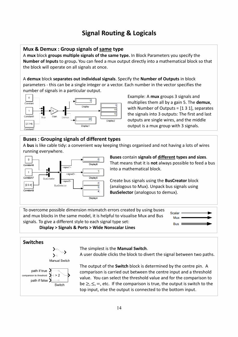
Signal Routing & Logicals

Mux & Demux : Group signals of same type A mux block groups multiple signals of the same type. In Block Parameters you specify the Number of Inputs to group. You can feed a mux output directly into a mathematical block so that the block will operate on all signals at once. A demux block separates out individual signals. Specify the Number of Outputs in block parameters - this can be a single integer or a vector. Each number in the vector specifies the number of signals in a particular output.

Example: A mux groups 3 signals and multiplies them all by a gain 5. The demux, with Number of Outputs = [1 3 1], separates the signals into 3 outputs: The first and last outputs are single wires, and the middle output is a mux group with 3 signals.

Buses : Grouping signals of different types A bus is like cable tidy: a convenient way keeping things organised and not having a lots of wires running everywhere.

Buses contain signals of different types and sizes. That means that it is not always possible to feed a bus into a mathematical block. Create bus signals using the BusCreator block (analogous to Mux). Unpack bus signals using BusSelector (analogous to demux).

To overcome possible dimension mismatch errors created by using buses and mux blocks in the same model, it is helpful to visualise Mux and Bus signals. To give a different style to each signal type set: Display > Signals & Ports > Wide Nonscalar Lines

Switches The simplest is the Manual Switch. A user double clicks the block to divert the signal between two paths. The output of the Switch block is determined by the centre pin. A comparison is carried out between the centre input and a threshold value. You can select the threshold value and for the comparison to be ≥, ≤, =, etc. If the comparison is true, the output is switch to the top input, else the output is connected to the bottom input.

15

Selectors : Accessing specific signals In MATLAB to access the 3rd and 6th elements of a vector, V say, we would use index notation: V([3 6]). Selectors are the Simulink equivalent of these indices in MATLAB:

Constant source with "Interpret vector parameters as 1-D" option checked

The selector above has been configured to extract the 3rd and the 6th element of the input vector. This has been done by setting: Number of Inputs = 6 and Index Vector = [3 6]. You can also configure selectors so that the Index Vector is obtained via an external input (select “Index Vector (port)” in the drop down menu). Selectors will also work higher dimensional arrays. It is important to note the dimensions of the quantities you are working with. Untick the box in the Selector Block Parameters “Interpret vector as 1-D” to change how the constant is interpreted. By setting Display > Signals & Ports > Signal Dimensions to on, we now see that the constant has been interpreted as a 2-D vector.

Constant source with "Interpret vector parameters as 1-D" option not checked;

Goto / From Blocks : Move signals without connecting wires Another way to move signals around is to use Goto and From blocks. Send a signal to a Goto block, where it is given a unique tag. Then a From block can be configured to use this same tag and access the signal. A simple example is given below. These blocks can be used to avoid complex signals crossing, and even work to get signals out of subsystems.

Compare To… These blocks compare a signal with either zero, a constant or another signal. The particular operation (greater than, equals to etc) is selected by a block parameter. The output is a Boolean.

Logic Operator The Logical Operator block carries out the same operation as a Boolean logic gate. The logic operation e.g. AND, OR, NOT etc is selected from block parameters. The first two blocks (above) are AND blocks with different block parameter settings. The first has default rectangular icon shape, the second has the icon shape set to distinctive. The last two are XOR with three inputs (rectangular and distinctive shape).

16

Integration and Differentiation There are continuous and discrete integrator and derivative blocks.

Continuous Integrator There are various ways of configuring integrators with extra functionality using block parameters:

By default, the Initial Condition is set within the block,

however it can be set as a block input. (set Initial Condition Source to External)

Limit the output to a maximum and minimum value

(tick Limit Output, adds saturation icon to block).

You can add an external reset signal, to force the output of the integrator back to its initial condi-

tion. You can configure the reset pin to act on a rising edge, falling edge or both.

Discrete Integrator For the discrete integrator block, you can specify whether to use forward or backward Euler, or the Trapezoidal method. As with the continuous integrator block you can specify in the block parameters if you want to define initial conditions externally or internally, set upper and lower limits and set up a reset condition. You can also define an input gain value.

Continuous Derivative The derivative block approximates the derivative of the input signal 𝑢 with respect to the time 𝑡, by computing a numerical difference. Here 𝛥𝑢 is the change in input value and 𝛥𝑡 is the change in time since the previous simulation (major) time step:

𝑦(𝑇𝑐𝑢𝑟𝑟𝑒𝑛𝑡) =Δ𝑢

Δ𝑡=

𝑢(𝑇𝑐𝑢𝑟𝑟𝑒𝑛𝑡) − 𝑢(𝑇𝑝𝑟𝑒𝑣𝑖𝑜𝑢𝑠)

𝑇𝑐𝑢𝑟𝑟𝑒𝑛𝑡 − 𝑇𝑝𝑟𝑒𝑣𝑖𝑜𝑢𝑠

The initial output for the block is zero.

Discrete Derivative

The discrete derivative block computes an optionally scaled discrete time derivative with output:

𝑦(𝑇𝑐𝑢𝑟𝑟𝑒𝑛𝑡) =𝐾𝑢(𝑇𝑐𝑢𝑟𝑟𝑒𝑛𝑡)

𝑇𝑠−

𝐾𝑢(𝑇𝑝𝑟𝑒𝑣𝑖𝑜𝑢𝑠)

𝑇𝑠

where 𝑇𝑠 is the fixed simulation time step.

Note on accuracy of derivatives: It is best practice to structure your models to use Integrators instead of Derivative blocks, as Integrator blocks have states that allow solvers to adjust step size and improve accuracy of the simulation. The derivative block output might be very sensitive to the dynamics of the entire model. The accuracy of the output signal depends on the size of the time steps taken in the simulation. Smaller steps allow a smoother and more accurate output, however unlike with blocks that have continuous states, the solver does not take smaller steps when the input to this block changes rapidly.

17

MATLAB & Simulink Working Together

While Simulink is useful for modelling and visualising processes such as feedback loops, detailed data analysis and generation of good quality figures is still best completed within MATLAB. You can run Simulink models and export the results to MATLAB or run Simulink models from MATLAB.

Exporting Simulink Data to MATLAB There are multiple ways to get data from a Simulink to MATAB:

Scope Block: You can enabling data logging from a Scope block within the Configuration

Menu Logging tab (see page 9).

To Workspace block: Once this block is used in your model, each time you run your model two vari-

ables are created in the MATLAB workspace:

tout – column vector of time steps

simout – variable storing simulation data

Use a Mux if you need more than one output. The simulation data can be of type timeseries, array or structure, as set in ‘Save Format’ in Block Parameters. Accessing your data in MATLAB depends on the variable type you set. After running the simulation command above, you can define the vector of time steps as:

and the columns of signal data as:

y = s.get(‘simout’) if ‘Save Format’ is array y = s.get(‘simout’).Data if ‘Save Format’ is structure y = s.get(‘simout’).signals.values if ‘Save Format’ is timeseries

Running Simulations from MATLAB You can also run your Simulink models using commands from MATLAB. The most basic way is to use the sim command with two outputs and one input (the model file name as a string):

where t is a column vector of time steps and y is a corresponding matrix with columns of signal data. The sim command can also be used with other inputs that allow the control of simulation run time for example, but only one output must be assigned. The extra inputs are known as ‘name-valued pairs’ as a condition is specified and then the value set. For example:

When using a single output, the Simulink model must also be set up to export data in some way, otherwise s will only give a vector of timesteps. This can be done by adding a ‘To Workspace’ Block, as described above, or adding Output Ports to the Simulink model.

t = s.get('tout')

[t,y]=sim('model')

s = sim('model',’StopTime’,’10’,’MaxStep’,’0.1’)

18

Examples Models

The following examples will hopefully give ideas for the best way to lay out models. While there is no right or wrong way, always prioritise readability.

Example 1: Dynamic Systems

The above shows the general approach to modelling dynamic systems. You calculate the force, use Newton’s 2nd law to calculate the acceleration, integrate to get the velocity and then integrate again to obtain the position. The above model is a general guide, it can get a bit more complicated. For example, the mass is required to calculate gravitational forces. It is also possible that the mass will be a function. For example, a rocket losses most of its mass as the fuel is burnt off.

19

Example 2: Ordinary Differential Equations (ODE)

The general rule for solving differential equations is to write the equation in terms of the highest differential. For example, consider the general second order equation below.

𝑦 + 𝑎�̈� + 𝑏�̇� + 𝑐𝑦 = 𝑓(𝑡) (1)

𝑦 = 𝑓(𝑡) − 𝑎�̈� − 𝑏�̇� − 𝑐𝑦

You then use integrators to obtain lower terms:

The right hand side of the equations is formed by feeding back these terms to form the expression required. Notice that the model contains no differentiators, even though we are modelling a differential equation. Models with differentiators tend to produce a lot of noise, so are avoided if possible. The next example is not linear or time invariant:

�̈� = �̇�2 − 𝑡𝑦 (2)

20

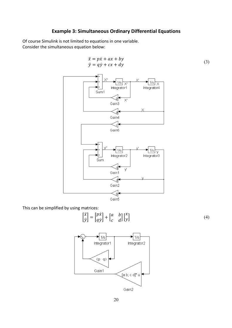
Example 3: Simultaneous Ordinary Differential Equations

Of course Simulink is not limited to equations in one variable. Consider the simultaneous equation below:

�̈� = 𝑝�̇� + 𝑎𝑥 + 𝑏𝑦�̈� = 𝑞�̇� + 𝑐𝑥 + 𝑑𝑦

(3)

This can be simplified by using matrices:

[�̈��̈�

] = [𝑝�̇�𝑞�̇�

] + [𝑎 𝑏𝑐 𝑑

] [𝑥𝑦] (4)

21

Example 4: Linear Systems

Many systems can be modelled by linear, time invariant (LTI) differential equations, such as equation 5 below.

𝑎3y⃛ + 𝑎2�̈� + 𝑎1�̇� + 𝑎0𝑦 = 𝑏2�̈� + 𝑏1�̇� + 𝑏0𝑥 (5)

where y is the output and x the input.

LTI systems can be represented by a transfer function:

𝐻(𝑠) =𝑌(𝑠)

𝑋(𝑠)=

𝑏2𝑠2 + 𝑏1𝑠 + 𝑏0

𝑎3𝑠3 + 𝑎2𝑠2 + 𝑎1𝑠 + 𝑎0

𝐻(𝑗𝜔) =𝑏2(𝑗𝜔)2 + 𝑗𝜔𝑏1 + 𝑏0

𝑎3(𝑗𝜔)3 + 𝑎2(𝑗𝜔)2 + 𝑗𝜔𝑎1 + 𝑎0

It is the convention in MATLAB to represent polynomial expressions with row vectors of the coefficients. So the numerator of the above transfer function is represented by [b2 b1 b0] and the denominator by [a3 a2 a1 a0]. Entering these two vectors to the appropriate block parameters of a transfer function block will produce the following block:

LTI transfer functions are used extensively in electronics to represent idealized electronic circuits. Take for example this circuit and its transfer function representation below:

𝐻(𝑠) =𝑉𝑜𝑢𝑡(𝑠)

𝑉𝑖𝑛(𝑠)=

𝑠𝜔𝑛

𝑠2 + 3s𝜔𝑛 + 𝜔𝑛2 (6)

The following model can be used to observe the behaviour in Simulink:

In the Transfer Function block parameters values are set with wn being a predefined variable in the MATLAB workspace: numerator = [wn 0] and denominator = [1 3*wn wn^2]

22

Poles and Zeros An alternative way of representing a transfer functions is to use the pole-zero description. If you solve the numerator polynomial you get the zeros. So called because the transfer function is zero at that value. If you solve the denominator polynomial, you get the poles. They are called poles because if you plot the absolute value of a transfer function, it looks a bit like a tent, with the poles being the location of the tent poles.

The transfer function from the circuit example can then be represented in its pole zero form:

𝐻(𝑠) = 𝐾(𝑠 − 𝑧1)(𝑠 − 𝑧2)

(𝑠 − 𝑝1)(𝑠 − 𝑝2)(𝑠 − 𝑝3) (7)

Where 𝑝𝑖 is a pole and 𝑧𝑖 is a zero and 𝐾 is a constant. You can model the transfer function in this form using a zero-pole block:

To configure this block you provide a vector for the numerator and the denominator. In this case the numerator is [z1 z2] and the denominator is [p1 p2 p3] and the gain is K.

Useful MATLAB functions: The MATLAB function roots will solve a polynomial, given the coefficients of the polynomial. The

function poly does the opposite. Given the roots of a polynomial, it will return the coefficients of

the polynomial.

The Signal Processing toolbox provides a number of functions to provide the coefficients required

to implement various filters. See help for butter, cheby1, cheby2 and besself.

The function freqs(B,A) will plot the frequency response of a system, where B is a vector of

the numerator coefficients and A is a vector of the denominator coefficients.

23

Example 5: Modelling Discrete Systems

A discrete signal has values only at discrete points in time. A sampled signal is always discrete. The sample period, T, is the time between two successive samples and sample frequency, fs, is 1/T.

You will need to set the Sample Time in Block Parameters for many of the blocks in the discrete library. Most blocks use ‘-1’ which is simply the inherited value from the model. Unfortunately, inherited sample time does not work for discrete models. If you find that you model is sampling at one second, regardless of the solver settings, then check the sample time of your blocks.

The fundamental component of a discrete system is a Unit delay. This delays the signal by one time period. In general, 𝑦𝑛 = 𝑥𝑛−1, as seen in the example below.

The Z transform replaces each delay by one sample with a multiplication by z -1:

𝑌(𝑧) = 𝑧−1𝑋(𝑧)

𝐻(𝑧) =𝑌(𝑧)

𝑋(𝑧)=

1

𝑧

There are other blocks in the discrete library that contain combinations of unit delays.

You can also use the Tapped Delay block:

24

Discrete Transfer Functions Continuous systems are described by differential equations, discrete systems are described by recurrence equation. Equation 8 below is a typical recurrence equation:

𝑎0𝑦𝑛 + 𝑎1𝑦𝑛−1 + 𝑎2𝑦𝑛−2 + 𝑎3𝑦𝑛−3 = 𝑏𝑜𝑥𝑛 + 𝑏1𝑥𝑛−1 + 𝑏2𝑥𝑛−2 (8)

where 𝑥 is the input and 𝑦 the output. Each unit delay is replace by z -1 in the Z transform.

(𝑎0 + 𝑎1𝑧−1 + 𝑎2𝑧−2 + 𝑎3𝑧−3)𝑌(𝑧) = (𝑏𝑜 + 𝑏1𝑧−1 + 𝑏2𝑧−2)𝑋(𝑧)

𝐻(𝑧) =𝑌(𝑧)

𝑋(𝑧)=

𝑏𝑜 + 𝑏1𝑧−1 + 𝑏2𝑧−2

𝑎0 + 𝑎1𝑧−1 + 𝑎2𝑧−2 + 𝑎3𝑧−3 (9)

which is the transfer function of a digital filter and is defined in terms of z -1. This can be represented in a Simulink model by the discrete filter block.

This block was produced by setting: numerator = [b0 b1 b2] and denominator = [a0 a1 a2 a3]

in the block parameters. Do not forget to set the sample time too.

An alternative form is to write the transfer function in terms of z. If we multiply top and bottom of equation 9 by z3 we get equation (10). You can represent this with the Transfer Function block or if you have the poles and zeros, the Zero-Pole block.

𝐻(𝑧) =𝑏𝑜𝑧3 + 𝑏1𝑧2 + 𝑏2𝑧

𝑎0𝑧3 + 𝑎1𝑧2 + 𝑎2𝑧1 + 𝑎3 (10)

Finite Impulse Response (FIR) digital filters do not have any poles. The recurrence equation:

𝑦𝑛 = 𝑏𝑜𝑥𝑛 + 𝑏1𝑥𝑛−1 + 𝑏2𝑥𝑛−2 (11)

gives the following Z transform and can be represented by the block especially for FIR filters:

𝑌(𝑧) = (𝑏𝑜 + 𝑏1𝑧−1 + 𝑏2𝑧−2)𝑋(𝑧)

𝐻(𝑧) =𝑌(𝑧)

𝑋(𝑧)= 𝑏𝑜 + 𝑏1𝑧−1 + 𝑏2𝑧−2 (12)

25

Simulink Shortcuts This section contains the short cut keys that can be used to build and edit your model. For more details select from the model menu bar Help ► Keyboard Shortcuts

OBJECT SELECTION SHORTCUTS

Select an object Click

Select more objects Shift+click

Select all objects Ctrl+A

Copy object Drag with right mouse button Ctrl+drag

Delete selected object Delete or Backspace

Cut Ctrl+X

Paste Ctrl+V

Undo Ctrl+Z

Redo Ctrl+Y

BLOCK SHORTCUTS

Search for blocks Click and type

Add text to model Double click and type

Move block Drag or Arrow keys

Resize block Drag handles in corners

Resize block, keeping same ratio of width and height

Shift + drag handle

Resize block from the center Ctrl + drag handle

Rotate block counterclockwise Ctrl + Shift + R

Flip block Ctrl+I

Rotate block clockwise Ctrl+R

Rotate block counterclockwise Ctrl+Shift+R

Connect blocks Drag from port to port

Select first block, Ctrl+click second block

Draw branch line Ctrl+drag line Right-mouse button+drag

Create subsystem from selected blocks Ctrl+G

Open selected subsystem Enter or Double click

Go to parent of selected subsystem Esc

SIMULATION SHORTCUTS

Open Configuration Parameters dialog box Ctrl+E

Update diagram Ctrl+D

Start simulation Ctrl+T

Stop simulation Ctrl+Shift+T

Build model (for code generation) Ctrl+B

26

SIGNALS SHORTCUTS

Name a signal line Double-click signal and type name

Delete signal label and name Delete characters in label or delete name in Signal Properties dialog box.

Delete signal label only Right-click label and select Delete Label.

Open signal label text box for edit Double-click signal line Click label

Move signal label Drag label to a new location on same signal line

Copy signal label Ctrl+drag signal label

Change the label font Select the signal line (not the label) and use Diagram > Format > Font Style

ZOOMING SHORTCUTS

Zoom in Ctrl + +

Zoom out Ctrl + -

Zoom to normal (100%) Ctrl + 0 or Alt + 1

Zoom with mouse Ctrl + scroll wheel

Zoom in on object Drag the Zoom button from the palette to the object

Fit diagram to screen Spacebar

Scroll view Arrow keys or Shift + arrow for larger pans

Scroll with mouse Spacebar + drag Hold the scroll wheel down and drag the mouse

27

The Solver: Zero-Crossing Options

A variable-step solver dynamically adjusts the time step size, causing it to increase when a variable is changing slowly and to decrease when the variable changes rapidly. This behaviour causes the solver to take many small steps in near a discontinuity because the variable is rapidly changing in this region. This improves accuracy but can lead to excessive simulation times. Simulink uses a technique known as zero-crossing detection to accurately locate a discontinuity without resorting to tiny time steps. Usually this technique improves simulation run time, but it can cause some simulations to halt before the intended completion time. Understanding how Simulink’s zero-crossing detection algorithms, adaptive and non-adaptive, work is beyond the scope of the course. The table below should help you overcome some errors associated with zero-crossing, particularly a halting model. Implementing most of the changes, involves using the Model Configuration Parameters dialog (MCP) box, accessed via the Cog symbol.

Possible Change... How to make this change... Rationale for making this change...

Increase the number of allowed zero crossings

Increase the Number of consecutive zero crossings on the Solver pane in the MCP box.

This may give your model enough time to resolve the zero crossing.

Disable zero-crossing detection for a specific block

First, clear the Enable zero-crossing detection check box on the block's parameter dialog box. Then, select Use local settings from the Zero-crossing control pull down on the Solver pane of the MCP box.

Locally disabling zero-crossing detection prevents a specific block from stopping the simulation because of excessive consecutive zero crossings. All other blocks continue to benefit from the increased accuracy that zero-crossing detection provides.

Disable zero-crossing detection for the entire model

Select Disable all from the Zero-crossing control pull down on the Solver pane of the MCP box.

This prevents zero crossings from being detected anywhere in your model.

Reduce the maximum step size

Enter a value for the Max step size option on the Solver pane of the MCP box.

This can insure the solver takes steps small enough to resolve the zero crossing. However, reducing the step size can increase simulation time, and is seldom necessary when using the Adaptive algorithm.

Use the Adaptive Algorithm

Select Adaptive from the Algorithm pull down on the Solver pane in the MCP box.

This algorithm dynamically adjusts the zero-crossing threshold, which improves accuracy and reduces the number of consecutive zero crossings detected. You can now specify Time tolerance and Signal threshold.

Relax the Signal threshold

Select Adaptive from the Algorithm pull down and increase the value of the Signal threshold option on the Solver pane in the MCP box.

The solver requires less time to precisely locate the zero crossing. This can reduce simulation time and eliminate an excessive number of consecutive zero-crossing errors. However, relaxing the Signal threshold may reduce accuracy.

28

Simulink Online Documentation

The full Simulink documentation is available from the help menu. You can obtain this from the MATLAB help, or you can go directly to the Simulink help. From the model menu bar select Help ► Simulink ► Simulink Help Block Documentation The easiest way of obtaining the documentation for a particular block is to hit the help button in the block parameters. An alternative is to select the block and then select Help ► Simulink ► Blocks & Blocksets Reference from the model menu bar. If no block is selected when you do this, then you will be given a list of all the blocks. You can then select the documentation you want from this list. At the top of the list, on the right hand side you can choose to display by Category or in Alphabetic order. In the Help Menu you will also find links to Web Resources Help ► Web Resources Particularly useful MATLAB Central which is the hub for the online MATLAB and Simulink community. Here you will find “MATLAB Answers” where people ask for support on MATLAB & Simulink. Once you become confident with MATLAB and Simulink you may wish to explore the File Exchange, where people upload custom files.

29

Further Examples

Simulink Onramp In MATLAB 2018b, you can complete the Simulink Onramp course created by MathWorks. It is around 3 hours of good quality content designed to introduce you to Simulink. It will give you more practice at a similar level to the exercises in this course. You can access this by installing MATLAB 2018b (see instructions on final pages of notes) and then downloading a toolbox available at

bit.ly/SimulinkOnRamp OR

https://uk.mathworks.com/matlabcentral/fileexchange/69056-simulink-onramp

Once installed, restart MATLAB, launch Simulink and click the link under Learn

Explore Simulink Examples Use the Examples Tab to explore different Simulink models ( File > New > Model…)

There is even a bouncing ball example so you can see a different approach to one you might have taken in the final exercise. Experiment with Simulink Dashboard Blocks Open the Fuel System Demo with the command: f open_system([matlabroot '\toolbox\simulink\simdemos\automotive\fuelsys\sldemo_fuelsys']) Read through the documentation, so that you understand how the model works: https://uk.mathworks.com/help/simulink/ug/tune-and-visualize-your-model-with-dashboard-blocks.html Explore the blocks by double clicking them to get a better understanding of how they work. Follow the instructions in the section Tune Parameters During Simulation to try editting the model.

30

Oxford University MATLAB Installation

1. VISIT UNIQUE WEB ADDRESS

To install MATLAB onto your computer, go to the web page http://bit.ly/OxUniMatlab OR

https://www.mathworks.com/login/identity/university?entityId=https://registry.shibboleth.ox.ac.uk/idp

Use your University of Oxford, single sign-on username and password.

2. CREATE UNIVERSITY LINKED MATHWORKS ACCOUNT

Then click on Create to make a MathWorks Account:

To register to use MATLAB, you need an Oxford University e-mail address such as firstname.lastname@eng.ox.ac.uk.

Fill in the rest of the form. The system will send you an e-mail, with a link you must click to verify. You can access your e-mail at https://outlook.office.com/owa/

Now you can access many resources: e.g. MATLAB Online, Mobile or Academy.

You can also download and install MATLAB for your personal computer. See the next page for details.

31

3. DOWNLOAD CHOOSEN MATLAB VERSION

After verification you will be taken directly to the MATLAB download page. (Also accessible by “My Account” and the Download Icon: )

Choose the most recent release (mac users see the table for guidance).

4. SELECT THE CORRECT INSTALLATION METHOD AND LICENSE

When you run the installer, you will be asked to select an Installation Method.

Select Log in with a MathWorks Account.

Later, you will be asked enter an e-mail address and password.

Use the e-mail address and password that you for your MathWorks account

When asked to Select a license, choose the license with the Individual Label.

Which MATLAB version for mac? Use the table on the right to choose the correct MATLAB release for your operating system.

To find which version of OSX you are using. On the Mac, Click on the apple in the far top left.

Select About this MAC

If you have any problems or queries, have a look at the MATLAB FAQ page: http://users.ox.ac.uk/~engs1643/matlab-faq.html

Mac Operating System MATLAB

High Sierra macOS 10.13 R2018a

Sierra macOS 10.12 R2018a

El Capitan OS X 10.11 R2018a

Yosemite OS X 10.10 R2017a

Mavericks OS X 10.9.5 R2015b

OS X 10.9 R2014b

Mountain Lion OS X 10.8 R2014b

Lion OS X 10.7.4 & above R2014b

OS X 10.7 R2012a or b

Snow Leopard OS X 10.6.4 & above R2012a or b

OS X 10.6.x R2010b

Leopard

OS X 10.5.8 & above R2010b

OS X 10.5.5 & above R2010a

OS X 10.5.x R2008b

Toolboxes: When asked to select the products, there are over 80 toolboxes available to install. If

you are using a standard broadband network connection at home, it will take many hours to

download all the toolboxes. To save time, select just MATLAB and the toolboxes you need. We

suggest MATLAB, Symbolic Math Toolbox and Simulink. You can run the installer again later to

add additional toolboxes.