An Introduction to using JAGS for Bayesian Regression Analysis Brief Introduction to Bayesian Regression.pdf · An Introduction to using JAGS for Bayesian Regression Analysis

An Introduction to using JAGS for Bayesian Regression Analysis

Kevin AndersonSupervised by Christian Iliadis

May 2, 2016

Contents

1 Preface 2

2 Background 22.1 Bayes’ Theorem . . . . . . . . . . . . . . . . . . . . . . . . . . . . . . . . . . . . . . . . . . . . 22.2 MCMC . . . . . . . . . . . . . . . . . . . . . . . . . . . . . . . . . . . . . . . . . . . . . . . . 3

3 Bayesian Regression 33.1 Basic Linear Model . . . . . . . . . . . . . . . . . . . . . . . . . . . . . . . . . . . . . . . . . . 33.2 Linear Model with Error Bars . . . . . . . . . . . . . . . . . . . . . . . . . . . . . . . . . . . . 83.3 Linear Model with Multiple Datasets and Systematic Error . . . . . . . . . . . . . . . . . . . 133.4 Nonlinear models . . . . . . . . . . . . . . . . . . . . . . . . . . . . . . . . . . . . . . . . . . . 19

3.4.1 Malus’s Law . . . . . . . . . . . . . . . . . . . . . . . . . . . . . . . . . . . . . . . . . 193.4.2 Growing Signal . . . . . . . . . . . . . . . . . . . . . . . . . . . . . . . . . . . . . . . . 213.4.3 The Slow Fourier Transform . . . . . . . . . . . . . . . . . . . . . . . . . . . . . . . . . 24

4 Choosing a Prior 274.1 Uninformative Priors . . . . . . . . . . . . . . . . . . . . . . . . . . . . . . . . . . . . . . . . . 274.2 Informative Priors . . . . . . . . . . . . . . . . . . . . . . . . . . . . . . . . . . . . . . . . . . 29

5 Notes 29

6 Modifying JAGS 306.1 Overview . . . . . . . . . . . . . . . . . . . . . . . . . . . . . . . . . . . . . . . . . . . . . . . 306.2 Installing Dependencies . . . . . . . . . . . . . . . . . . . . . . . . . . . . . . . . . . . . . . . 306.3 JAGS functions . . . . . . . . . . . . . . . . . . . . . . . . . . . . . . . . . . . . . . . . . . . . 316.4 ArrayFunction . . . . . . . . . . . . . . . . . . . . . . . . . . . . . . . . . . . . . . . . . . . . 31

6.4.1 the constructor . . . . . . . . . . . . . . . . . . . . . . . . . . . . . . . . . . . . . . . . 316.4.2 evaluate . . . . . . . . . . . . . . . . . . . . . . . . . . . . . . . . . . . . . . . . . . . . 316.4.3 checkParameterDim . . . . . . . . . . . . . . . . . . . . . . . . . . . . . . . . . . . . . 326.4.4 checkParameterValue . . . . . . . . . . . . . . . . . . . . . . . . . . . . . . . . . . . . 326.4.5 dim . . . . . . . . . . . . . . . . . . . . . . . . . . . . . . . . . . . . . . . . . . . . . . 32

6.5 C++ Implementation . . . . . . . . . . . . . . . . . . . . . . . . . . . . . . . . . . . . . . . . 326.5.1 SFactor.cc . . . . . . . . . . . . . . . . . . . . . . . . . . . . . . . . . . . . . . . . . . . 326.5.2 SFactor.h . . . . . . . . . . . . . . . . . . . . . . . . . . . . . . . . . . . . . . . . . . . 35

6.6 Recompiling JAGS . . . . . . . . . . . . . . . . . . . . . . . . . . . . . . . . . . . . . . . . . . 356.7 Appendix . . . . . . . . . . . . . . . . . . . . . . . . . . . . . . . . . . . . . . . . . . . . . . . 36

6.7.1 Timings . . . . . . . . . . . . . . . . . . . . . . . . . . . . . . . . . . . . . . . . . . . . 366.7.2 Code . . . . . . . . . . . . . . . . . . . . . . . . . . . . . . . . . . . . . . . . . . . . . . 39

1

1 Preface

This paper is an introduction to constructing Bayesian regression models using the R programming languageand the R package rjags. Familiarity with the R language and basic statistical background (means, standarddeviations, etc) are necessary to understand the material.

The intent of this paper is to show how easy it is to fit complex regression models to experimental datawith rjags. The techniques applied in this paper are surprisingly powerful, given their simplicity.

## Last modified on

## Mon May 2 16:29:11 2016

## rjags info:

## Loading required package: coda

## Linked to JAGS 4.2.0

## Loaded modules: basemod,bugs

## R version 3.2.4 Revised (2016-03-16 r70336)

## Platform: x86_64-pc-linux-gnu (64-bit)

## Running under: Debian GNU/Linux stretch/sid

##

## locale:

## [1] LC_CTYPE=en_US.UTF-8 LC_NUMERIC=C

## [3] LC_TIME=en_US.UTF-8 LC_COLLATE=en_US.UTF-8

## [5] LC_MONETARY=en_US.UTF-8 LC_MESSAGES=en_US.UTF-8

## [7] LC_PAPER=en_US.UTF-8 LC_NAME=C

## [9] LC_ADDRESS=C LC_TELEPHONE=C

## [11] LC_MEASUREMENT=en_US.UTF-8 LC_IDENTIFICATION=C

##

## attached base packages:

## [1] stats graphics grDevices utils datasets base

##

## other attached packages:

## [1] rjags_4-6 coda_0.18-1 knitr_1.12.3

##

## loaded via a namespace (and not attached):

## [1] magrittr_1.5 formatR_1.2.1 tools_3.2.4 stringi_1.0-1

## [5] grid_3.2.4 methods_3.2.4 stringr_1.0.0 lattice_0.20-33

## [9] evaluate_0.8

2 Background

2.1 Bayes’ Theorem

First, some notation: for an event A, the probability of the event occurring is given by P (A). For instance,the probabilities of an unbiased coin flip can be written as P (heads) = 0.5 and P (tails) = 0.5.

In many cases, we wish to know the conditional probability of an event. P (A|B) represents the probabilityof event A occurring, given that event B occurs. To give an example of the difference between this andstandard probability, if today is Wednesday (event A), the probability of tomorrow being Thursday (eventB) is P (B|A) = 1, while without the condition, the probability is random: P (B) = 1/7.

The whole subject of Bayesian Inference rests on a mathematical rule called Bayes’ theorem:

P (H|E) =P (E|H)P (H)

P (E)

2

Here, H stands for a hypothesis to be tested and E stands for the evidence (data). The right side containsthree terms. P (E|H) is the likelihood of measuring the evidence, assuming that the hypothesis is true. Thetwo probabilities P (H) and P (E) are called priors or prior distributions and represent relevant knowledgebeyond the dataset itself. They are called “priors” because we know these probabilities before doing theanalysis.

The left side of Bayes’ theorem reads “The probability of H given the evidence”, which represents exactlywhat we are interested in – how likely is this hypothesis, according to the data that we collected? Thisprobability is known as the posterior or the posterior distribution. In this paper, we’ll focus on fitting modelparameters to datasets, and so what we are interested in are real numbers: slopes, intercepts, standarddeviations, etc. These of course lie on the real axis and are continuous, and so the posterior for some modelwill be probability distributions for each parameter.

In general, each of these terms can be arbitrarily complex, and so actually using Bayes’ theorem foranalytic calculation is often impractical. To get around this, we use a numerical technique called MarkovChain Monte Carlo.

2.2 MCMC

Monte Carlo methods are algorithms that use randomly generated numbers to estimate numbers that aretoo hard to calculate analytically. A common use case for Monte Carlo techniques is evaluating complexmultidimensional integrals. We won’t cover the theory of Markov Chain Monte Carlo here, as many resourcesare available for this. Suffice to say, we will generate Markov Chains from which the posterior distributionscan be calculated.

3 Bayesian Regression

3.1 Basic Linear Model

The overall idea with using rjags is to define a model structure, give this, our datasets, and prior distributionsto the MCMC engine, and get back posterior distributions of specified parameters.

First, the package needs to be loaded, and we may as well set a seed for the random number generator sothat our results are reproducible:

library(rjags)

set.seed(1)

Now let’s make a basic model to test rjags. The simplest realistic example is a linear relationship withsome y-scatter. Let’s make an artificial dataset for testing:

## Create an artificial dataset:

true_slope = 1

true_intercept = -5

true_sigma = 2

N = 50

x = runif(N,0,10)

y = rnorm(N,true_slope * x + true_intercept, true_sigma)

At least for now, we should take a look at our data before analyzing it, just to make sure it is how weexpect it to be:

plot(x,y)

3

●

●

●

●

●

●

●

●

●

●

●●

●

●

●

●

●

●

●

●

●

●

●

●

● ●

●

●

●●

●

●

●●

●

●

●

●

●

●

●

●

●

●

●

●

●

●●

●

0 2 4 6 8 10

−6

−4

−2

02

46

x

y

Now let’s talk about the model we will use. We are modeling the data as linear with gaussian scatter:

yi ∼ N (axi + b, σ2)

To actually implement this model, we will need to express it in the JAGS langauge. The JAGS languageis a little different from normal programming languages like R. It is a declarative language, meaning thatthe code you write is not followed as a sequence of steps, but rather as a description of logic. For instance,the line y.hat[i] = a * x[i] + b does not evaluate the right side and set the left side equal to it, as R

would. Instead, this code only specifies the model structure that JAGS should use.For now, the model code will be separated into two sections. The first is for specifying priors on our

parameters of interest. Here, we are interested in the slope a , intercept b , and standard deviation sigma

of our dataset. The second section is for describing how our different variables are related to each other.

Then, the whole chunk of JAGS code is wrapped in model{...} and passed into the JAGS engine.

For this dataset, the priors might be as follows. The slope a we expect to be non-negative and no greater

than 5, so we could use a uniform density between 0 and 5. The intercept b could be anywhere between

±10, and the scatter’s standard deviation sigma is expected to be between 0 and 3. Note that the choice

of priors is domain specific and not the emphasis here, but we have chosen priors that include the “true”values.

Let’s write the JAGS code for this model and capture it into a string:

model_string = "

model {## priors:

a ~ dunif(0,5)

4

b ~ dunif(-10,10)

sigma ~ dunif(0,3)

## structure:

for (i in 1:N) {y[i] ~ dnorm(a * x[i] + b, pow(sigma, -2))

}}

"

Density functions in JAGS always start with “d”: dunif for uniform density, dnorm for gaussian density,

dlnorm for lognormal density, etc. The tildes are read as “is distributed as”. For instance, a ~ dunif(0,5)

is read as “the variable a is distributed uniformly between 0 and 5”.In the structure block, we have a traditional for loop. This allows us to relate each y value to each

x value such that each y value is normally distributed around the line a ∗ x + b with standard deviation

sigma . For historical reasons, JAGS distribution functions use a “precision” that is defined as one over the

variance. Usually it is more convenient to speak in terms of standard deviation and variance, so most modelswill have a small conversion between standard deviation and precision included.

Note that the order of lines is somewhat unimportant – the priors could have been included after thestructure and it would make no difference.

Now that we have a model structure and some data, we can give this to JAGS and see what comesback. Normally the JAGS engine wants the model structure in a separate file, but to keep it easy we’ll use atextConnection instead. This allows us to create a fake file whose contents are the model string we created

above, and we’ll give this to JAGS instead.Now, we want to give our model structure and data to JAGS and get back the output of the MCMC

process to analyze.

model = jags.model(file = textConnection(model_string),

data = list('x' = x,

'y' = y,

'N' = N),

n.chains = 1,

n.adapt = 1000,

inits = list('.RNG.name' = 'base::Mersenne-Twister',

'.RNG.seed' = 1))

## Compiling model graph

## Resolving undeclared variables

## Allocating nodes

## Graph information:

## Observed stochastic nodes: 50

## Unobserved stochastic nodes: 3

## Total graph size: 313

##

## Initializing model

This has created a model, and printed some information that is not particularly interesting. We can thenactually generate a Markov chain with

output = coda.samples(model = model,

variable.names = c("a", "b", "sigma"),

n.iter=1000,

thin=1)

5

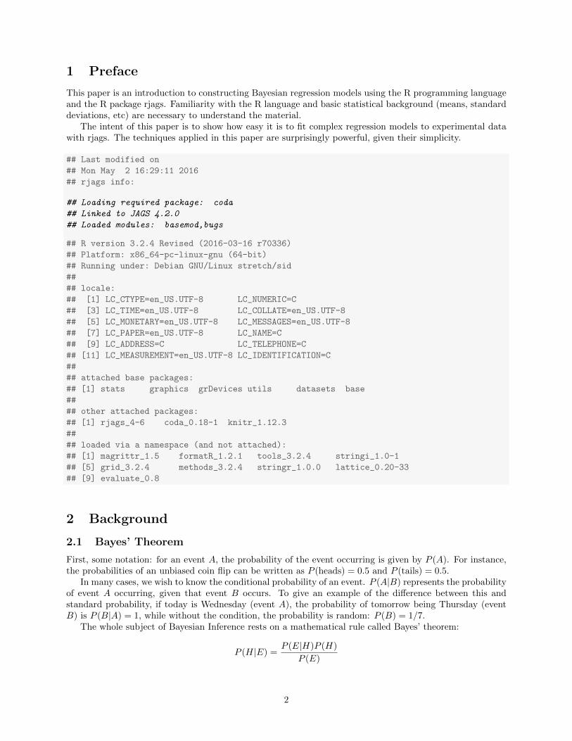
We get back an object output that contains the Markov chain. First, as always in R, have a look at the

summary of it:

print(summary(output))

##

## Iterations = 1001:2000

## Thinning interval = 1

## Number of chains = 1

## Sample size per chain = 1000

##

## 1. Empirical mean and standard deviation for each variable,

## plus standard error of the mean:

##

## Mean SD Naive SE Time-series SE

## a 1.015 0.09858 0.003117 0.010918

## b -4.905 0.57907 0.018312 0.063502

## sigma 1.891 0.19389 0.006131 0.007875

##

## 2. Quantiles for each variable:

##

## 2.5% 25% 50% 75% 97.5%

## a 0.8372 0.9484 1.013 1.078 1.220

## b -6.0694 -5.2835 -4.876 -4.513 -3.857

## sigma 1.5659 1.7509 1.876 2.016 2.306

This gives us information about the distributions of the parameters we asked JAGS to calculate ( a , b ,

and sigma ). Notice that the means for each parameter are quite close to the true values. We can also see

this visually:

plot(output)

6

1000 1200 1400 1600 1800 2000

0.8

1.0

1.2

Iterations

Trace of a

0.8 1.0 1.2 1.4

01

23

4

Density of a

N = 1000 Bandwidth = 0.02572

1000 1200 1400 1600 1800 2000

−6.

5−

5.0

−3.

5

Iterations

Trace of b

−7 −6 −5 −4 −30.

00.

30.

6

Density of b

N = 1000 Bandwidth = 0.1532

1000 1200 1400 1600 1800 2000

1.4

2.0

2.6

Iterations

Trace of sigma

1.5 2.0 2.5

0.0

1.0

2.0

Density of sigma

N = 1000 Bandwidth = 0.05162

We see mixing diagrams on the left, and posterior distributions on the right. The mixing diagrams appearqualitatively acceptable, and the posterior distributions are centered on or quite near the true values of 1, -5,and 2, respectively. The model has successfully recovered the values we used to create the data. The total,self-contained code for this is as follows:

library(rjags)

set.seed(1)

true_slope = 1

true_intercept = -5

true_sigma = 2

N = 50

x = runif(N,0,10)

y = rnorm(N,true_slope * x + true_intercept, true_sigma)

plot(x,y)

model_string = "

model {

7

## priors:

a ~ dunif(0,5)

b ~ dunif(-10,10)

sigma ~ dunif(0,3)

## structure:

for (i in 1:N) {y[i] ~ dnorm(a * x[i] + b, pow(sigma, -2))

}}"



'y' = y,

'N' = N),

n.chains = 1,

n.adapt = 1000,


'.RNG.seed' = 1))


variable.names = c("a", "b", "sigma"),

n.iter=1000,

thin=1)

print(summary(output))

plot(output)

The rest of the examples in this paper will follow more or less the same format: create or load in somedata, define the model, pass it to JAGS, and have a look at the output.

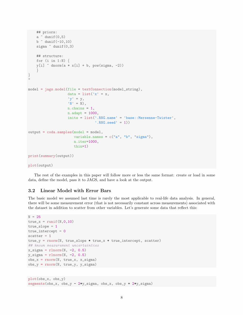
3.2 Linear Model with Error Bars

The basic model we assumed last time is rarely the most applicable to real-life data analysis. In general,there will be some measurement error (that is not necessarily constant across measurements) associated withthe dataset in addition to scatter from other variables. Let’s generate some data that reflect this:

N = 25

true_x = runif(N,0,10)

true_slope = 1

true_intercept = 0

scatter = 1

true_y = rnorm(N, true_slope * true_x + true_intercept, scatter)

## known measurement uncertainties

x_sigma = rlnorm(N, -2, 0.5)

y_sigma = rlnorm(N, -2, 0.5)

obs_x = rnorm(N, true_x, x_sigma)

obs_y = rnorm(N, true_y, y_sigma)

plot(obs_x, obs_y)

segments(obs_x, obs_y - 2*y_sigma, obs_x, obs_y + 2*y_sigma)

8

segments(obs_x - 2*x_sigma, obs_y, obs_x + 2*x_sigma, obs_y)

●

●

●

●

●

●

●

●

●

●

●

●

●

●

●

●

●

●

●

●

●

●

●

●●

2 4 6 8

02

46

810

obs_x

obs_

y

Clearly, the group scatter is larger than the individual measurement error bars allow, implying that one ormore unmeasured variables are influencing the y values. The model we’ll use is a linear relationship betweeny and x, with (uniform) measurement error on both y and x and additional scatter in y. The JAGS code isas follows:

model_string = "

model {## priors:

a ~ dunif(0,5)

b ~ dunif(-10,10)

scatter ~ dunif(0,3)

## structure:

for (i in 1:N) {## the true x:

x[i] ~ dunif(0,10)

## the observed x:

obs_x[i] ~ dnorm(x[i], pow(x_sigma[i],-2))

## y, as it would be if it only depended on the true x:

y[i] = a*x[i] + b

## y, with the effect of the unmeasured confounding variable

9

y_scatter[i] ~ dnorm(y[i], pow(scatter,-2))

## y, with the confounding variable, with observational error:

obs_y[i] ~ dnorm(y_scatter[i], pow(y_sigma[i],-2))

}}

"

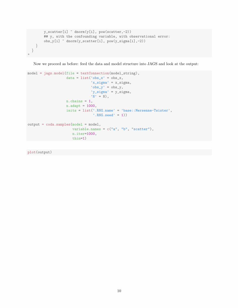
Now we proceed as before: feed the data and model structure into JAGS and look at the output:


data = list('obs_x' = obs_x,

'x_sigma' = x_sigma,

'obs_y' = obs_y,

'y_sigma' = y_sigma,

'N' = N),

n.chains = 1,

n.adapt = 1000,


'.RNG.seed' = 1))


variable.names = c("a", "b", "scatter"),

n.iter=1000,

thin=1)

plot(output)

10

1000 1400 1800

0.8

1.2

Iterations

Trace of a

0.8 1.0 1.2 1.4

02

4

Density of a

N = 1000 Bandwidth = 0.02111

1000 1400 1800

−1.

51.

0

Iterations

Trace of b

−2 −1 0 1 2

0.0

0.6

Density of b

N = 1000 Bandwidth = 0.118

1000 1400 1800

0.6

1.4

Iterations

Trace of scatter

0.6 1.0 1.4 1.8

0.0

1.5

Density of scatter

N = 1000 Bandwidth = 0.04457

Again, the model has reproduced the parameters used to generate the data. What would happen if weran the code again, but increased the measurement uncertainty?

## these values are the same as in the previous model:

#N = 25

#true_x = runif(N,0,10)

#true_slope = 1

#true_intercept = 0

#scatter = 0.25

#true_y = rnorm(N, true_slope * true_x + true_intercept, scatter)

## known measurement uncertainties (much larger than before)

x_sigma = rlnorm(N, 1, 0.5)

y_sigma = rlnorm(N, 1, 0.5)

obs_x = rnorm(N, true_x, x_sigma)

obs_y = rnorm(N, true_y, y_sigma)

plot(obs_x, obs_y)

segments(obs_x, obs_y - 2*y_sigma, obs_x, obs_y + 2*y_sigma)

segments(obs_x - 2*x_sigma, obs_y, obs_x + 2*x_sigma, obs_y)

11

●

●●●

●

●

●

●

●

●●

●

●

●

●

●

●

●

●● ●

●

●

●

●

−10 −5 0 5 10 15

−5

05

1015

obs_x

obs_

y

This time, the uncertainty bars are much larger, and you would think that very little information couldbe extracted from these data. Using the same model as before, let’s see what the output looks like:

12

2000 6000 10000

0.0

1.0

Iterations

Trace of a

0.0 0.5 1.0 1.5

0.0

1.5

Density of a

N = 10000 Bandwidth = 0.03878

2000 6000 10000

−2

26

Iterations

Trace of b

−2 0 2 4 6

0.00

0.25

Density of b

N = 10000 Bandwidth = 0.2251

2000 6000 10000

0.0

2.0

Iterations

Trace of scatter

0.0 1.0 2.0 3.0

0.0

0.6

Density of scatter

N = 10000 Bandwidth = 0.1161

Here, the number of MCMC iterations has been increased to 10,000. With the 1,000 iterations usedbefore, the mixing diagrams did not appear robust. The slope and intercept posterior distributions are notas smooth and are wider than before, and the scatter posterior is maximized far from the true value. Asexpected, using uninformative data results in uninformative posteriors.

3.3 Linear Model with Multiple Datasets and Systematic Error

Systematic error is something that is typically difficult to deal with in statistical analysis, but is easy here.First, let’s examine the case when the systematic error is proportional to x . Imagine we have two data setswith qualitatively different slopes:

## generate some data

slope = 2

intercept = 5

N1 = 20

shift1 = 0.7;

obs_x1 = runif(N1,0,10)

err_y1 = runif(N1, 0.1, 0.2)

obs_y1 = shift1 * rnorm(N1, slope * obs_x1 + intercept, err_y1)

N2 = 30

shift2 = 1.3;


13

err_y2 = runif(N2, 0.1, 0.2)

obs_y2 = shift2 * rnorm(N2, slope * obs_x2 + intercept, err_y2)

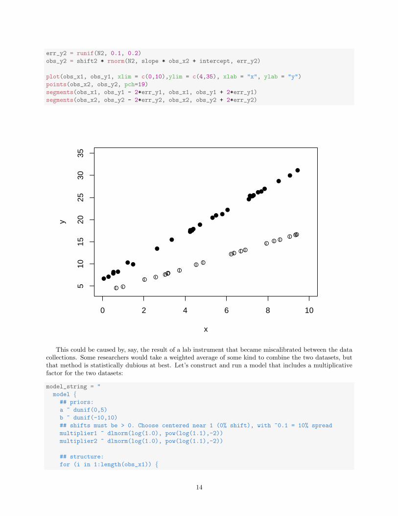
plot(obs_x1, obs_y1, xlim = c(0,10),ylim = c(4,35), xlab = "x", ylab = "y")

points(obs_x2, obs_y2, pch=19)

segments(obs_x1, obs_y1 - 2*err_y1, obs_x1, obs_y1 + 2*err_y1)


●

●

●

●

●●

●●

●

●

●

●●

●●

●

●

●

●

●

0 2 4 6 8 10

510

1520

2530

35

x

y

●

●

●

●

●●

●

●

●

●●

●

●

●

●

●

●

●

●

●

●

●

●

●

●

●

●

●

●

●

This could be caused by, say, the result of a lab instrument that became miscalibrated between the datacollections. Some researchers would take a weighted average of some kind to combine the two datasets, butthat method is statistically dubious at best. Let’s construct and run a model that includes a multiplicativefactor for the two datasets:

model_string = "

model {## priors:

a ~ dunif(0,5)

b ~ dunif(-10,10)

## shifts must be > 0. Choose centered near 1 (0% shift), with ~0.1 = 10% spread

multiplier1 ~ dlnorm(log(1.0), pow(log(1.1),-2))

multiplier2 ~ dlnorm(log(1.0), pow(log(1.1),-2))

## structure:

for (i in 1:length(obs_x1)) {

14

y1[i] = multiplier1 * (a*obs_x1[i] + b)

obs_y1[i] ~ dnorm(y1[i], pow(err_y1[i],-2))

}for (i in 1:length(obs_x2)) {

y2[i] = multiplier2 * (a*obs_x2[i] + b)


}}

"


data = list('obs_x1' = obs_x1,

'obs_x2' = obs_x2,

'obs_y1' = obs_y1,

'obs_y2' = obs_y2,

'err_y1' = err_y1,

'err_y2' = err_y2),

n.chains = 1,

n.adapt = 1000,


'.RNG.seed' = 1))


variable.names = c("a", "b", "multiplier1", "multiplier2"),

n.iter=500000,

#n.iter =10000,

thin=1)

Note that the number of iterations has been increased to 500,000 from the standard 10,000. This model’sadded complexity required more iterations for the Markov chains to converge. The posterior distributionsare amazingly accurate:

plot(output)

15

The slope, intercept, and both systematic error multipliers are all centered exactly on their true values.Now, let’s look at an additive systematic error. Imagine we have two datasets, each with a positive systematicerror (implying that taking a weighted average would not help very much).

## generate some data

slope = 2

intercept = 5

N1 = 20

shift1 = 1.5;


err_y1 = runif(N1, 0.1, 0.2)

obs_y1 = shift1 + rnorm(N1, slope * obs_x1 + intercept, err_y1)

N2 = 30

16

shift2 = 3;


err_y2 = runif(N2, 0.1, 0.2)

obs_y2 = shift2 + rnorm(N2, slope * obs_x2 + intercept, err_y2)

plot(obs_x1, obs_y1, xlim = c(0,10),ylim = c(5,25), xlab = "x", ylab = "y")

points(obs_x2, obs_y2, pch=19)



●

●

●●

●

●

●

●

●

●

●

●

●

●

●

●

●

●

●●

0 2 4 6 8 10

510

1520

25

x

y

●●

●

●●

●

●

●

●

●

●

●

●●

●

●

●●

●

●

●

●

●

●

●

●

●

●●

●

The model will be similar to before:

model_string = "

model {## priors:

a ~ dunif(0,5)

b ~ dunif(-10,10)

shift1 ~ dnorm(0, 1)

shift2 ~ dnorm(0, 1)

## structure:

for (i in 1:length(obs_x1)) {y1[i] = shift1 + (a*obs_x1[i] + b)


17

}for (i in 1:length(obs_x2)) {

y2[i] = shift2 + (a*obs_x2[i] + b)


}}

"


data = list('obs_x1' = obs_x1,

'obs_x2' = obs_x2,

'obs_y1' = obs_y1,

'obs_y2' = obs_y2,

'err_y1' = err_y1,

'err_y2' = err_y2),

n.chains = 1,

n.adapt = 1000,


'.RNG.seed' = 1))


variable.names = c("a", "b", "shift1", "shift2"),

n.iter = 500000,

thin=1)

Again the number of iterations has been increased to 500,000.

plot(output)

18

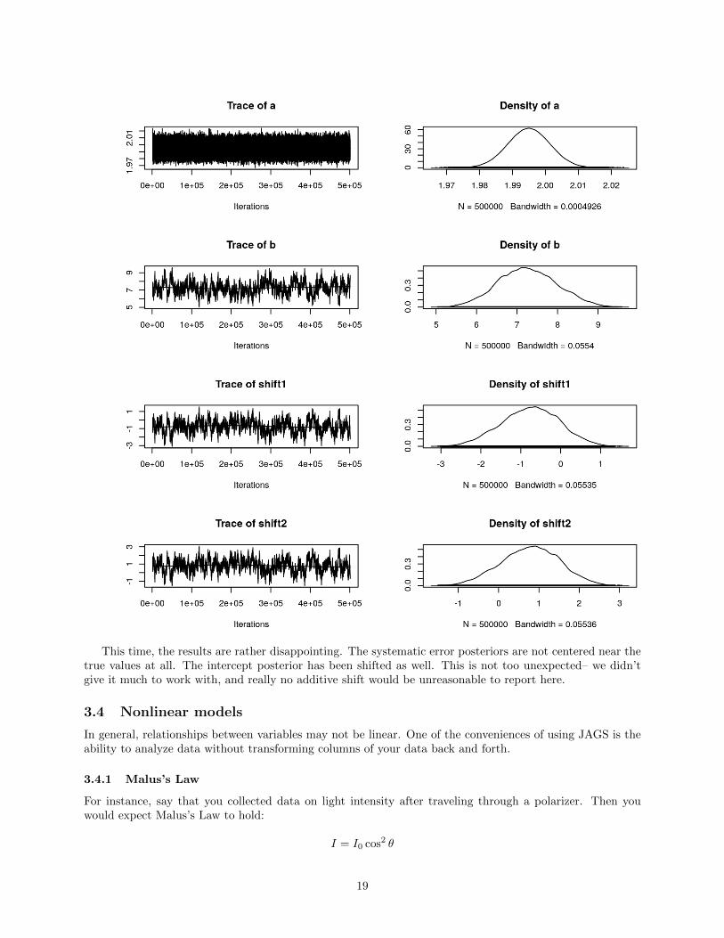
This time, the results are rather disappointing. The systematic error posteriors are not centered near thetrue values at all. The intercept posterior has been shifted as well. This is not too unexpected– we didn’tgive it much to work with, and really no additive shift would be unreasonable to report here.

3.4 Nonlinear models

In general, relationships between variables may not be linear. One of the conveniences of using JAGS is theability to analyze data without transforming columns of your data back and forth.

3.4.1 Malus’s Law

For instance, say that you collected data on light intensity after traveling through a polarizer. Then youwould expect Malus’s Law to hold:

I = I0 cos2 θ

19

If you measured I as a function of θ, perhaps the goal is to calculate the value of I0, or to verify that itindeed varies with cos2 θ rather than cos2 aθ for a 6= 1.

## theta in degrees, I in lux. data taken from

## http://www.physicslabs.umb.edu/Physics/sum13/182_Exp1_Sum13.pdf

data.table = read.table(header = TRUE, text =

"theta I

0 24.45

10 23.71

20 21.59

30 18.34

40 14.35

50 10.10

60 6.11

70 2.86

80 0.74

90 0.00")

# convert to radians

data.table$theta = data.table$theta * pi/180

Now, let’s write the model to test the two parameters I0 and a, and get an idea of what the scatter aroundMalus’s Law is:

model_string = "

model {## priors:

a ~ dunif(0,10)

I0 ~ dunif(0,50)

sigma ~ dunif(0,100)

for (i in 1:length(theta)) {I[i] ~ dnorm(I0 * (cos(a*theta[i]))^2, pow(sigma,-2))

}}

"


data = list('theta' = data.table$theta,

'I' = data.table$I),

n.chains = 1,

n.adapt = 1000,


'.RNG.seed' = 1))


variable.names = c("a", "I0", "sigma"),

n.iter =10000,

thin=1)

plot(output)

20

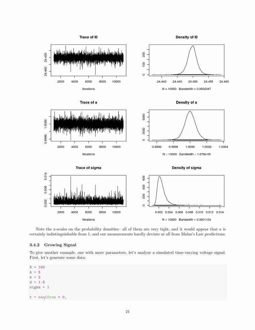
Note the x-scales on the probability densities– all of them are very tight, and it would appear that a iscertainly indistinguishable from 1, and our measurements hardly deviate at all from Malus’s Law predictions.

3.4.2 Growing Signal

To give another example, one with more parameters, let’s analyze a simulated time-varying voltage signal.First, let’s generate some data:

N = 100

A = 5

w = 2

d = 1.5

sigma = 1

t = seq(from = 0,

21

to = 10,

length.out = N)

y = rnorm(N,

A*t*cos(w*t + d),

sigma)

plot(t,y)

●●●●●●●

●●●●●●●

●●●●

●●

●●●●●●

●●●●●

●●●

●●●●

●●●●

●●●●

●

●

●

●

●●●●●●●●

●

●●

●

●

●

●

●

●

●

●●●●●

●●

●

●

●

●

●

●

●

●

●●

●●●●

●

●

●

●

●

●

●

●

●

●

●

0 2 4 6 8 10

−40

−20

020

40

t

y

Note that now we have four parameters: an amplitude, a frequency, a phase shift, and the noise. Themodel is simple:

model_string = "

model {A ~ dunif(0,10)

w ~ dunif(0,10)

d ~ dunif(-3.14, 3.14)

sigma ~ dunif(0,10)

for (i in 1:length(t)) {y[i] ~ dnorm(A*t[i]*cos(w*t[i] + d), pow(sigma, -2))

}}"


data = list('t' = t,

22

'y' = y),

n.chains = 1,

n.adapt = 1000)


variable.names = c("A", "w", "sigma", "d"),

n.iter = 10000,

thin=1)

And the output is surprisingly good:

plot(output)

23

3.4.3 The Slow Fourier Transform

Just for fun, let’s see if we can emulate the Fourier Transform with JAGS. First, let’s make a plausible signalto transform. Choose some random lattice points, then spline between them and sample the interpolation:

set.seed(2)

anchor.x = 1:10

anchor.y = rnorm(10,0,0.5)

x = seq(from=0,to=10,by=0.1)

spline_values = spline(x = anchor.x, y = anchor.y, xout = x, method = "fmm")

y = spline_values$y

plot(anchor.x, anchor.y)

lines(x,y)

●

●

●

●

●

●

●

●

●

●

2 4 6 8 10

−0.

50.

00.

51.

0

anchor.x

anch

or.y

Looks like a reasonable signal to analyze. Now, let’s assume that we can fit a model of the form

y(x) ≈5∑

n=1

[an sin(nx) + bn cos(nx)]

This is going to be a pretty rough approximation, since we are only using 5 terms and not including then = 0 contribution. No matter. Let’s now define the model. The values for an and bn probably won’t be toolarge, since the signal’s amplitude is relatively small. Hopefully, the difference between our approximatedsignal and the real thing will be relatively small as well.

24

N_terms = 5

model_string = "

model {## priors:

for(i in 1:N){a[i] ~ dunif(-100,100)

b[i] ~ dunif(-100,100)

}for(i in 1:length(x)) {

err[i] ~ dunif(0,100)

}

# loop over x

for (i in 1:length(x)) {# loop over frequencies

for (j in 1:N){y.hat[i,j] = a[j]*sin(j*x[i]) + b[j]*cos(j*x[i])

}y[i] ~ dnorm(sum(y.hat[i,]), pow(err[i],-2))

}}

"



'y' = y,

'N' = N_terms),

n.chains = 1,

n.adapt = 1000,


'.RNG.seed' = 1))


variable.names = c("a", "b", "err"),

n.iter = 10000,

thin=1)

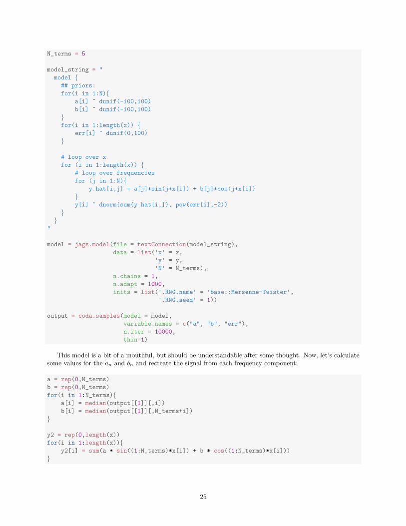
This model is a bit of a mouthful, but should be understandable after some thought. Now, let’s calculatesome values for the an and bn and recreate the signal from each frequency component:

a = rep(0,N_terms)

b = rep(0,N_terms)

for(i in 1:N_terms){a[i] = median(output[[1]][,i])

b[i] = median(output[[1]][,N_terms+i])

}

y2 = rep(0,length(x))

for(i in 1:length(x)){y2[i] = sum(a * sin((1:N_terms)*x[i]) + b * cos((1:N_terms)*x[i]))

}

25

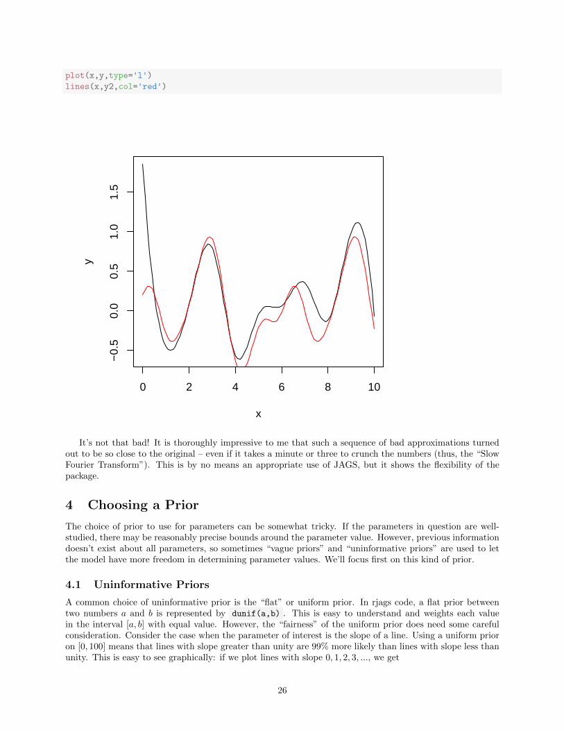
plot(x,y,type='l')

lines(x,y2,col='red')

0 2 4 6 8 10

−0.

50.

00.

51.

01.

5

x

y

It’s not that bad! It is thoroughly impressive to me that such a sequence of bad approximations turnedout to be so close to the original – even if it takes a minute or three to crunch the numbers (thus, the “SlowFourier Transform”). This is by no means an appropriate use of JAGS, but it shows the flexibility of thepackage.

4 Choosing a Prior

The choice of prior to use for parameters can be somewhat tricky. If the parameters in question are well-studied, there may be reasonably precise bounds around the parameter value. However, previous informationdoesn’t exist about all parameters, so sometimes “vague priors” and “uninformative priors” are used to letthe model have more freedom in determining parameter values. We’ll focus first on this kind of prior.

4.1 Uninformative Priors

A common choice of uninformative prior is the “flat” or uniform prior. In rjags code, a flat prior betweentwo numbers a and b is represented by dunif(a,b) . This is easy to understand and weights each valuein the interval [a, b] with equal value. However, the “fairness” of the uniform prior does need some carefulconsideration. Consider the case when the parameter of interest is the slope of a line. Using a uniform prioron [0, 100] means that lines with slope greater than unity are 99% more likely than lines with slope less thanunity. This is easy to see graphically: if we plot lines with slope 0, 1, 2, 3, ..., we get

26

plot(0,0)

for(i in 0:100){abline(0,i,col='red');

}

●

−1.0 −0.5 0.0 0.5 1.0

−1.

0−

0.5

0.0

0.5

1.0

0

0

Clearly, more steep lines exist than shallow lines, so this prior is probably less “fair” than you might havethought. A more fair alternative might be a uniform prior on φ, the angle between the line and the x-axis.Then the slope corresponding to each φ is b = tanφ (because slope is ∆y/∆x = sinφ/ cosφ). To see thisgraphically:

plot(0,0)

phi_array = seq(from = 0, to = pi/2, by = 0.1)

for(phi in phi_array){abline(0,tan(phi),col='red');

}

27

●

−1.0 −0.5 0.0 0.5 1.0

−1.

0−

0.5

0.0

0.5

1.0

0

0

So, if a uniformly-weighted prior is desired, sometimes it takes a bit of thought to achieve. It is a goodidea to think about whether you would rather be totally ignorant of the scale of the parameter rather thanthe value of the parameter – if you are ignorant of the parameter’s order of magnitude, then it is as likelyto be in [1, 10] as it is to be in [100, 1000]. This corresponds to a logarithmic decaying prior, which could becreated as a uniform prior on the power of ten and then taking the logarithm for the parameter value.

In the past, people have put a lot of effort into find the “best” non-informative prior to use. The currentconcensus is that there is not one single uninformative prior that is the best to use for all models, thoughsome fields do have standard default priors.

Vague priors are usually very broad in the sense that they cover a large amount of the parameter’s possiblevalues. Examples of this include a wide uniform distribution and a Gaussian with large variance. A vagueprior may still have some information; for instance, using a wide lognormal distribution will require theposterior to be non-negative.

4.2 Informative Priors

If some information about the parameters is already known before the data analysis, this can (and should)be encoded in the prior. For example, if previous experiments have estimated the value of the parameterof interest, you might use a prior of a Gaussian centered on the existing estimate. Strictly non-negativeparameters can be described with a lognormal distribution, and in general the more flexible distributions (eggamma) can be used with carefully chosen shape parameters to get a wide range of shapes.

5 Notes

There are a few tricks to help get good results with JAGS. For example, the time-varying signal had aphase shift included, and the prior was chosen to be dunif(-3.14,3.14) rather than dunif(0,6.28) .Sometimes, the Markov Chain can “get stuck” and fail to sample accurately, and the choice of prior canaffect this.

Another way to avoid this problem is by specifying reasonable initial values for each parameter with theinits variable. If you do not specify the initial value for a parameter, JAGS will try to pick an appropriate

28

starting value. It usually works well, but can fail for some models.

6 Modifying JAGS

6.1 Overview

JAGS has the standard functions built into its model description language – log, sin, etc. However, morecomplex models may require custom domain-specific functions. Unfortunately, JAGS doesn’t provide a wayto include custom functions if the function can’t be implemented in the model itself as a combination ofthe builtins. For instance, a nuclear physics model might require calculation of Coulomb wavefunctions withsome given parameters. Existing fortran codes exist for this, and they are a thousand lines or more long,meaning that implementing them in the model directly is not feasible.

This document shows the process of creating new JAGS functions that can be used in a model description.They can use existing executables or be self-contained. This involves recompiling JAGS with the new functionadded in, and so the process of installing dependencies, compilers, etc will also be covered.

This document was written for JAGS version 4.2.0, R version 3.0.2, and R packages rjags 4-6 and coda0.18-1, running on Ubuntu 14.04. It may be helpful for more recent versions of these packages, but thingstend to change over time.

6.2 Installing Dependencies

This was originally done on a remote VPS, but a standard personal computer will also suffice. Theseinstructions assume a Debian-based GNU/Linux OS, as I have no experience with writing code on Mac OSXor Windows computers.

First, if your computer does not have much ram, you may want to enable a swapfile. This will allow yourcomputer to start using hard drive space as a (much slower) replacement for ram if it runs out. RunningJAGS models is not very memory-intensive, but compiling the JAGS source code can take a decent amount.This may not be necessary for you, but if you run into “memory full” issues later, this is one solution. Thefollowing commands at a bash terminal will create a 2GB swapfile that will persist until the computer nextshuts down:

fallocate -l 2G /swapfile

chmod 600 /swapfile

mkswap /swapfile

swapon /swapfile

To make the swapfile persist across reboots, use

echo '/swapfile none swap sw 0 0' >> /etc/fstab

Now, onto the actual dependencies. I started with a clean Ubuntu 14.04 installation. After installing Rwith

sudo apt-get install r-base-core

I installed the following packages to compile the JAGS source code:

sudo apt-get install make gcc g++ gfortran liblapack-dev r-base-core

sudo apt-get install autoconf automake libtool libltdl7-dev libcppunit-dev

At the time of writing, JAGS is hosted on SourceForge. The source code can be downloaded with abrowser, and then unpacked with a file manager, or in the terminal:

wget 'https://sourceforge.net/projects/mcmc-jags/files/JAGS/4.x/Source/JAGS-4.2.0.tar.gz/download'

tar -xvf download

rm download

29

Now, to compile and install JAGS without any modifications:

cd JAGS-4.2.0

./configure

make

sudo make install

If make throws errors, it might be that the linking path is wrong. If running the command

/sbin/ldconfig -p | grep jags

doesn’t print anything, then open /etc/ld.so.conf with your favorite text editor and insert the line

include /usr/local/lib

at the bottom. Save the file, and run /sbin/ldconfig to load the new configuration file. Then try make

again.Finally, to install the R-language bindings to JAGS,

Rscript -e "install.packages('rjags');"

6.3 JAGS functions

The JAGS source code defines several types of functions. By looking in /JAGS-4.2.0/src/include/function,you can see several class definition files – ArrayFunction.h, VectorFunction.h, ScalarVectorFunction.h,etc. These describe the types of the function parameters and return variables – ScalarVectorFunction takesvector arguments and returns a scalar, for instance. In our case, we wanted a function that accepts threescalar values and returns a 2-D array, so we chose to implement an ArrayFunction. Other function typeswill have different methods that need defining.

6.4 ArrayFunction

ArrayFunction defines several virtual methods that our code must implement. They describe the inputs andoutputs of the function in addition to what the function actually does.

6.4.1 the constructor

If you look at ArrayFunction.h, you can see that the constructor takes two parameters, a string name and anunsigned int npar. These correspond to the name that you want to be able to use in JAGS model descriptionsand the number of parameters that the function will take. In our case, we want to call the function sfactor

and it takes three parameters.

6.4.2 evaluate

The first method is evaluate, which defines the actual function definition. It has the parameters of a doublepointer value, a vector of double pointers args, and a vector of vectors of unsigned ints dims. The argumentvalue is a pointer to a region of memory for the return value – because ArrayFunction is supposed to bea very generic template, the specific details of how to use that memory is up to you. Note: JAGS arraysare stored in column-major order (like Fortran), not row-major order like C++ in general! The size of thismemory region is defined by the return value of the dim function.

The args parameter contains the arguments that the model description gave to the function. It is avector of double pointers, and so each element of the vector can represent an array. The dimensions of thesearrays must be accepted by checkParameterDim. In our case, we want it to be three scalars, so each elementof the args vector should point to only one double value.

The dims parameter provides the dimensions of the arrays in args. In our case, they should be all onesbecause our parameters are scalars, but in general they define the shape of the memory regions pointed toin args.

30

6.4.3 checkParameterDim

The method checkParameterDim checks whether the function parameters are correct. It has one argument,a vector of vectors of unsigned ints dims. The outer vector has npar (the parameter of the constructor)elements, and each subvector contains the dimensions of the corresponding argument to your function. Ourfunction accepts only scalars, so we use this function to check that all our arguments are scalars.

6.4.4 checkParameterValue

The method checkParameterValue is used to check whether the parameter values lie in the function’sdomain. Our function did not require any constraints on the parameter values, so it always returned true.

6.4.5 dim

The method dim is used to tell JAGS how much memory to allocate for given input values. In our case, weare outsourcing the calculations to a fortran code that returns a table with 99 rows and 2 columns, so wereturn a 2-element vector containing the values 99 and 2.

6.5 C++ Implementation

Now, onto the specifics of implementing a new function in C++. All existing functions are located in

JAGS-4.2.0/src/modules/bugs/functions

and we will put our code there as well. A JAGS function has two files: a main .cc file that defines thebodies of the functions mentioned above, and a header file .h that is more or less just boilerplate. To begin,it is easiest to copy the .cc and .h files of a function that already exists and is the same type as yours.We want an ArrayFunction, and so we could copy, for instance, Transpose.cc and Transpose.h, becauseTranpose inherits from ArrayFunction. Note: when in JAGS-4.2.0/src/modules/bugs/functions/, youcan use grep ArrayFunction * to find all functions that contain the phrase “ArrayFunction”.

After copying an existing function, we can modify the new files to fit our needs. In SFactor.cc andSFactor.h, the first thing to do is change all the Transposes to SFactors, so that #include "Transpose.h"

turns into #include "SFactor.h", Transpose::evaluate becomes SFactor::evaluate, and so on. Themethod parameters and return types should all stay the same.

6.5.1 SFactor.cc

Now let’s talk about method bodies. The methods are more or less independent, and so we’ll discuss theirimplementation individually.

6.5.1.1 the constructor Our JAGS function will be named sfactor and will take three parameters, sowe define our constructor as

SFactor::SFactor ()

: ArrayFunction ("sfactor", 3)

{

}

6.5.1.2 evaluate evaluate is the big function. Our objective is to provide a bridge between JAGS andan existing pre-compiled Fortran77 executable binary. The executable has an input file that contains all theparameter values used in the calculation and creates an output file with the 99x2 table of calculated values.The idea of this method is to create the input file with the three parameter values given to it by JAGS,execute the binary, and parse the table from the output file to return to JAGS.

Because we’ll be reading and writing files, we’ll need a few libraries. At the top of SFactor.cc, we havethe following lines:

31

#include <iostream>

#include <fstream>

#include <string>

#include <stdlib.h>

First, we have to get the three parameter values. Recall that args is a vector of double pointers. In ourcase, these pointers are pointing to single values (or equivalently, 1x1 arrays), so to access them, we simplyuse

double resonance_energy = args[0][0];

double proton_width = args[1][0];

double gamma_width = args[2][0];

Now, we write them to the binary’s input file, called “extrappg.in”. The file also contains values for manyother parameters, but those are treated as constants in this analysis, so we will hardcode them. The inputfile is assumed to be in a certain order, which must be preserved by this code:

// open the fortran input file for writing

std::ofstream paramfile;

paramfile.open ("extrappg.in");

paramfile << "17O+p ! title\n";

paramfile << "17 1.0078 ! mass target, projectile MT,MP\n";

paramfile << "8 1 ! charge target, projectile ZT,ZP\n";

paramfile << "1.25 ! radius parameter r0 (fm) R0\n";

paramfile << resonance_energy << " ! resonance energy (MeV) ER ***\n";

paramfile << "2.5 0.5 2.0 ! spins target, projectile, resonance JT,JP,JR\n";

paramfile << "5.6065 ! reaction Q-value (MeV) Q\n";

paramfile << "1 ! orbital angular momentum of resonance LP\n";

paramfile << proton_width << " ! proton width at ER (MeV) GAMP ***\n";

paramfile << gamma_width << " ! gamma widths at ER (MeV) GAMG ***\n";

paramfile << "0.00 ! proton spectroscopic factor C2S\n";

paramfile << "0.00 ! dim. single-particle reduced width at ER (formal) THSP\n";

paramfile << "1.887 ! excitation energy of final state (MeV) EXF\n";

paramfile << "1.00 ! gamma-ray branching ratio BG\n";

paramfile << "1 ! gamma-ray multipolarity LG\n";

paramfile << "0.02 1.0 0.01 ! start energy, final energy, step size (MEV) ES,EF,SS\n";

paramfile << "0 ! (1) exact calculation; (else) Thomas approximation;\n";

paramfile.close();

Now that the input file is written, we can run the external executable, which we assume is called s_factor.It is assumed to be in the same working directory as your R session. If this is not the case, you’ll have toprovide a full filepath to it.

// now that the parameter file is written, run the fortran executable

int retcode = system("./s_factor");

The return value retcode signals whether the process completed successfully or exited with an error. Intrue bad-practice style, we’ll ignore it here. Note that calling outside executables in this way will have ourcode wait until the external process finishes and returns. In this case, this is exactly what we want.

Now, we must read the table of values from the Fortran’s output file, called extrappg.out. The outputfile contains 14 lines of diagnostic info before getting to the table, at which point it has 99 lines of data, eachline containing two numbers separated by a space.

//read the fortran executable's output file:

std::string line;

std::ifstream ifile ("extrappg.out");

32

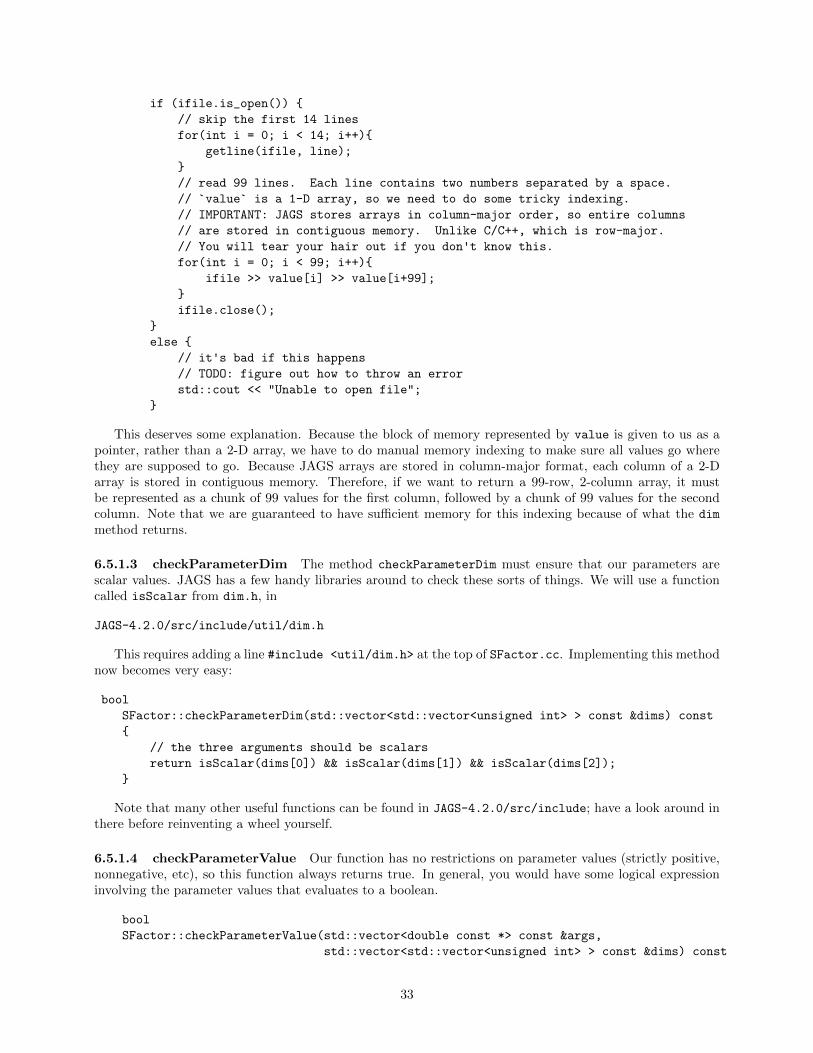
if (ifile.is_open()) {

// skip the first 14 lines

for(int i = 0; i < 14; i++){

getline(ifile, line);

}

// read 99 lines. Each line contains two numbers separated by a space.

// `value` is a 1-D array, so we need to do some tricky indexing.

// IMPORTANT: JAGS stores arrays in column-major order, so entire columns

// are stored in contiguous memory. Unlike C/C++, which is row-major.

// You will tear your hair out if you don't know this.

for(int i = 0; i < 99; i++){

ifile >> value[i] >> value[i+99];

}

ifile.close();

}

else {

// it's bad if this happens

// TODO: figure out how to throw an error

std::cout << "Unable to open file";

}

This deserves some explanation. Because the block of memory represented by value is given to us as apointer, rather than a 2-D array, we have to do manual memory indexing to make sure all values go wherethey are supposed to go. Because JAGS arrays are stored in column-major format, each column of a 2-Darray is stored in contiguous memory. Therefore, if we want to return a 99-row, 2-column array, it mustbe represented as a chunk of 99 values for the first column, followed by a chunk of 99 values for the secondcolumn. Note that we are guaranteed to have sufficient memory for this indexing because of what the dim

method returns.

6.5.1.3 checkParameterDim The method checkParameterDim must ensure that our parameters arescalar values. JAGS has a few handy libraries around to check these sorts of things. We will use a functioncalled isScalar from dim.h, in

JAGS-4.2.0/src/include/util/dim.h

This requires adding a line #include <util/dim.h> at the top of SFactor.cc. Implementing this methodnow becomes very easy:

bool

SFactor::checkParameterDim(std::vector<std::vector<unsigned int> > const &dims) const

{

// the three arguments should be scalars

return isScalar(dims[0]) && isScalar(dims[1]) && isScalar(dims[2]);

}

Note that many other useful functions can be found in JAGS-4.2.0/src/include; have a look around inthere before reinventing a wheel yourself.

6.5.1.4 checkParameterValue Our function has no restrictions on parameter values (strictly positive,nonnegative, etc), so this function always returns true. In general, you would have some logical expressioninvolving the parameter values that evaluates to a boolean.

bool

SFactor::checkParameterValue(std::vector<double const *> const &args,

std::vector<std::vector<unsigned int> > const &dims) const

33

{

// TODO: should any parameters be eg strictly positive?

return true;

}

6.5.1.5 dim dim tells JAGS what the dimensions of the output of evaluate should be. In our case, weknow that we will be returning a 2-D, 99x2 array of doubles. dim returns a vector of unsigned ints, witheach element corresponding to a dimension of an array. By convention, it seems that JAGS code assumesdimension vectors to contain first the number of rows, and then the number of columns, and so our dim willlook like

std::vector<unsigned int>

SFactor::dim(std::vector <std::vector<unsigned int> > const &dims,

std::vector <double const *> const &values) const

{

// the size of the table that the fortran code calculates is 99 row by 2 col

vector<unsigned int> ans(2);

ans[0] = 99;

ans[1] = 2;

return ans;

}

6.5.2 SFactor.h

The header file is much easier to implement. More or less just changing everything to fit your function’sname is all that’s necessary. Also, be sure that the #ifndef line has a unique identifier that won’t matchany other function’s.

6.6 Recompiling JAGS

Now that you’ve defined a function that JAGS can talk to, we have to tell JAGS about it. At the time ofwriting, there are two configuration files that must be edited. The first is found in

JAGS-4.2.0/src/modules/bugs/functions/Makefile.am

This file is a template used to generate a real makefile during the compilation process. Any functions youcreate that you want to be available in a JAGS model description must be listed here. There are two longlists in this file, one for .cc files and one for .h files. Just append your two new files to the ends of theselists.

The second file that requires editing is

JAGS-4.2.0/src/modules/bugs/bugs.cc

This file is a long list of #include statements. Scrolling down the file, there will be a list of all thefunctions we saw before, with lines like #include <functions/Transpose.h>. Add a similar line for your.h file in this list (eg, #include <functions/SFactor.h>).

Then, farther down the file, there will be a long list of lines like insert(new Transpose);. Add a newline for your function (eg, insert(new SFactor);).

After editing these two files, go back to the top level of the JAGS directory (JAGS-4.2.0 here), and runautoreconf --force --install to regenerate new configuration files from the templates you just edited.Then run the configure program in this directory with ./configure. After this, we are done configuring,and can proceed with make and sudo make install as before.

Note that the autoreconf --force --install and ./configure only need to be done after you editthe configuration templates Makefile.am and bugs.cc. After doing this once, you can skip those steps ifyou edit your new function’s .cc and .h files and go straight to the make and sudo make install. Afterthis, using the rjags library in R will point to the new custom version of JAGS.

34

6.7 Appendix

6.7.1 Timings

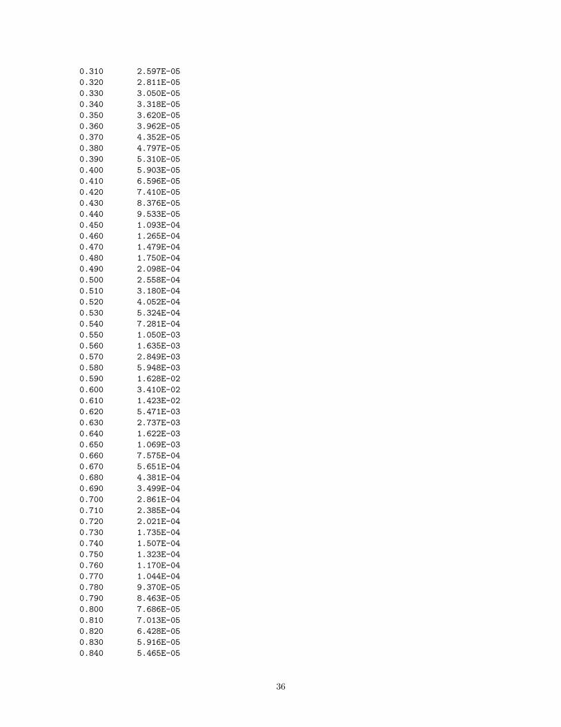
As a test, we used the extrappg Fortran binary to generate an output table for known parameters. Somenoise was then added to the data and used in JAGS to try to recreate the original parameter values. Thecode and results are shown below:

library(rjags)

# parameters used to generate the data:

# MT,MP,ZT,ZP = 17. 1. 9. 1.

# R0 (fm) =1.25

# LP,LG = 0 1

# GAMP,GAMG (MeV)= .180E-01 .250E-07

# ER,Q,EXF (MeV) = .600 3.924 1.887

# JT,JP,JR =2.5 .53.0

# THSP,C2S = .000 .000

# BG = 1.0000

# so the analysis should return

# ER = 0.600

# GAMP = 0.180e-01

# GAMG = 0.250e-07

df1 = read.table(header = TRUE, text =

" E S

0.020 4.883E-06

0.030 5.110E-06

0.040 5.351E-06

0.050 5.607E-06

0.060 5.878E-06

0.070 6.166E-06

0.080 6.473E-06

0.090 6.799E-06

0.100 7.147E-06

0.110 7.518E-06

0.120 7.914E-06

0.130 8.338E-06

0.140 8.792E-06

0.150 9.279E-06

0.160 9.802E-06

0.170 1.036E-05

0.180 1.097E-05

0.190 1.162E-05

0.200 1.233E-05

0.210 1.310E-05

0.220 1.393E-05

0.230 1.483E-05

0.240 1.581E-05

0.250 1.688E-05

0.260 1.806E-05

0.270 1.935E-05

0.280 2.076E-05

0.290 2.233E-05

0.300 2.406E-05

35

0.310 2.597E-05

0.320 2.811E-05

0.330 3.050E-05

0.340 3.318E-05

0.350 3.620E-05

0.360 3.962E-05

0.370 4.352E-05

0.380 4.797E-05

0.390 5.310E-05

0.400 5.903E-05

0.410 6.596E-05

0.420 7.410E-05

0.430 8.376E-05

0.440 9.533E-05

0.450 1.093E-04

0.460 1.265E-04

0.470 1.479E-04

0.480 1.750E-04

0.490 2.098E-04

0.500 2.558E-04

0.510 3.180E-04

0.520 4.052E-04

0.530 5.324E-04

0.540 7.281E-04

0.550 1.050E-03

0.560 1.635E-03

0.570 2.849E-03

0.580 5.948E-03

0.590 1.628E-02

0.600 3.410E-02

0.610 1.423E-02

0.620 5.471E-03

0.630 2.737E-03

0.640 1.622E-03

0.650 1.069E-03

0.660 7.575E-04

0.670 5.651E-04

0.680 4.381E-04

0.690 3.499E-04

0.700 2.861E-04

0.710 2.385E-04

0.720 2.021E-04

0.730 1.735E-04

0.740 1.507E-04

0.750 1.323E-04

0.760 1.170E-04

0.770 1.044E-04

0.780 9.370E-05

0.790 8.463E-05

0.800 7.686E-05

0.810 7.013E-05

0.820 6.428E-05

0.830 5.916E-05

0.840 5.465E-05

36

0.850 5.065E-05

0.860 4.709E-05

0.870 4.390E-05

0.880 4.104E-05

0.890 3.846E-05

0.900 3.613E-05

0.910 3.401E-05

0.920 3.208E-05

0.930 3.031E-05

0.940 2.870E-05

0.950 2.721E-05

0.960 2.584E-05

0.970 2.458E-05

0.980 2.341E-05

0.990 2.233E-05

1.000 2.132E-05")

sigma = 0.001

x = df1$E

y = rnorm(length(x), df1$S, sigma)

# so the analysis should return

# ER = 0.600

# GAMP = 0.180e-01

# GAMG = 0.250e-07

model_string = "

model {

ER ~ dunif(0.5,0.7)

GAMP ~ dunif(0.1e-01, 0.2e-01)

GAMG ~ dunif(0.1e-07, 0.3e-07)

# sigma is zero if it gets the other parameters right

sigma ~ dunif(0,10)

# a 99x2 table of E and S(E)

table = sfactor(ER, GAMP, GAMG)

for (i in 1:length(E)) {

S.hat[i] = interp.lin(E[i], table[1:99,1], table[1:99,2])

S[i] ~ dnorm(S.hat[i], pow(sigma,-2))

}

}

"


data = list('E' = x,

'S' = y),

n.chains = 1,

n.adapt = 1000)


variable.names = c("ER", "GAMP", "GAMG", "sigma"),

n.iter=3000,

37

thin=1)

The quantiles of the parameter values are shown below. Note that they nicely include the original trueparameter values of ER = 0.600, GAMG = 0.250e-07, GAMP = 0.180e-01, and sigma = 1e-3.

2.5% 25% 50% 75% 97.5%

ER 5.995e-01 6.001e-01 6.004e-01 6.007e-01 6.012e-01

GAMG 2.308e-08 2.422e-08 2.489e-08 2.556e-08 2.675e-08

GAMP 1.600e-02 1.693e-02 1.748e-02 1.802e-02 1.900e-02

sigma 9.454e-04 1.034e-03 1.084e-03 1.137e-03 1.262e-03

I ran this code on a single-core, 1GB ram computer with a solid-state harddrive. The model consumed apretty small amount of ram, and as we discussed, it consumed about 20-25% CPU, indicating that 75-80%of its time is spent on filesystem operations rather than direct cpu calculations. I used 3000 iterations, andthe timings were

real 4m42.614s

user 1m8.469s

sys 3m29.102s

6.7.2 Code

For reference, the complete SFactor.cc and SFactor.h files are included here:SFactor.cc:

#include "SFactor.h"

#include <config.h>

#include <cmath>

// isScalar()

#include <util/dim.h>

#include <iostream>

#include <fstream>

#include <string>

#include <stdlib.h>

using std::vector;

namespace jags {

namespace bugs {

/**

* @short Matrix- or array-valued function

*

* Array-valued functions are the most general class of function. The

* arguments of an array-valued function, and the value may be a

* scalar, vector, or array.

*

* We use ArrayFunction here because there is no more specific class

* that accepts scalars and returns vectors

*/

SFactor::SFactor ()

38

: ArrayFunction ("sfactor", 3)

{

}

/**

* Evaluates the function.

*

* @param value array of doubles which contains the result of

* the evaluation on exit

* @param args Vector of arguments.

* @param dims Respective dimensions of each element of args.

*/

void

SFactor::evaluate(double *value,

std::vector<double const *> const &args,


{

// parameters to be written to the fortran input file

double resonance_energy = args[0][0];

double proton_width = args[1][0];

double gamma_width = args[2][0];

// open the fortran input file for writing

std::ofstream paramfile;

paramfile.open ("extrappg.in");

paramfile << "17O+p ! title\n";

paramfile << "17 1.0078 ! mass target, projectile MT,MP\n";

paramfile << "8 1 ! charge target, projectile ZT,ZP\n";

paramfile << "1.25 ! radius parameter r0 (fm) R0\n";

paramfile << resonance_energy << " ! resonance energy (MeV) ER ***\n";

paramfile << "2.5 0.5 2.0 ! spins target, projectile, resonance JT,JP,JR\n";

paramfile << "5.6065 ! reaction Q-value (MeV) Q\n";

paramfile << "1 ! orbital angular momentum of resonance LP\n";

paramfile << proton_width << " ! proton width at ER (MeV) GAMP ***\n";

paramfile << gamma_width << " ! gamma widths at ER (MeV) GAMG ***\n";

paramfile << "0.00 ! proton spectroscopic factor C2S\n";

paramfile << "0.00 ! dim. single-particle reduced width at ER (formal) THSP\n";

paramfile << "1.887 ! excitation energy of final state (MeV) EXF\n";

paramfile << "1.00 ! gamma-ray branching ratio BG\n";

paramfile << "1 ! gamma-ray multipolarity LG\n";

paramfile << "0.02 1.0 0.01 ! start energy, final energy, step size (MEV) ES,EF,SS\n";

paramfile << "0 ! (1) exact calculation; (else) Thomas approximation;\n";

paramfile.close();

// now that the parameter file is written, run the fortran executable

int retcode = system("./s_factor");

//read the fortran executable's output file:

std::string line;

std::ifstream ifile ("extrappg.out");

if (ifile.is_open()) {

39

// skip the first 14 lines

for(int i = 0; i < 14; i++){

getline(ifile, line);

}

// read 99 lines. Each line contains two numbers separated by a space.

// `value` is a 1-D array, so we need to do some tricky indexing.

// IMPORTANT: JAGS stores arrays in column-major order, so entire columns

// are stored in contiguous memory. Unlike C, which is row-major.

// You will tear your hair out if you don't know this.

for(int i = 0; i < 99; i++){

ifile >> value[i] >> value[i+99];

}

ifile.close();

}

else {

// it's really bad if this happens

// TODO: figure out how to throw an error

std::cout << "Unable to open file";

}

}

/**

* Checks whether dimensions of the function parameters are correct.

*

* @param dims Vector of length npar denoting the dimensions of

* the parameters, with any redundant dimensions dropped.

*/

bool

SFactor::checkParameterDim(std::vector<std::vector<unsigned int> > const &dims) const

{

// the three arguments should be scalars

return isScalar(dims[0]) && isScalar(dims[1]) && isScalar(dims[2]);

}

/**

* Checks whether the parameter values lie in the domain of the

* function. The default implementation returns true.

*/

bool

SFactor::checkParameterValue(std::vector<double const *> const &args,


{

// TODO: should any parameters be eg strictly positive?

return true;

}

/**

* Calculates what the dimension of the return value should be,

* based on the arguments.

*

40

* @param dims Vector of Indices denoting the dimensions of the

* parameters. This vector must return true when passed to

* checkParameterDim.

*

* @param values Vector of pointers to parameter values.

*/


SFactor::dim(std::vector <std::vector<unsigned int> > const &dims,

std::vector <double const *> const &values) const

{

// the size of the table that the fortran code calculates is 99 row by 2 col

vector<unsigned int> ans(2);

ans[0] = 99;

ans[1] = 2;

return ans;

}

}}

SFactor.h:

#ifndef S_FACTOR_H_

#define S_FACTOR_H_

#include <function/ArrayFunction.h>

namespace jags {

namespace bugs {

/**

* @short Astronomical S Factors

* SFactor returns the astronomical S-factor as a function of energy. It

* returns a 99x2 table where column 1 is energy and column 2 is the S-factor.

* It requires a fortran executable to perform the calculations.

* <pre>

* table = sfactor(ER, GAMP, GAMG)

* </pre>

*/

class SFactor : public ArrayFunction

{

public:

SFactor ();

void evaluate(double *x, std::vector<double const *> const &args,

std::vector<std::vector<unsigned int> > const &dims)

const;

bool checkParameterDim(std::vector<std::vector<unsigned int> > const &dims) const;


dim(std::vector<std::vector<unsigned int> > const &dims,

std::vector<double const *> const &values) const;

bool checkParameterValue(std::vector<double const *> const &args,

std::vector<std::vector<unsigned int> > const &dims) const;

};

}}

41

Documents

An Introduction to using JAGS for Bayesian Regression Analysis Brief Introduction to Bayesian Regression.pdf · An Introduction to using JAGS for Bayesian Regression Analysis