Embed Size (px)
Citation preview

An Introduction to theAnalysis of Slender Structures
Angelo Simone

An Introduction to theAnalysis of Slender Structures
Angelo Simone


An Introduction to theAnalysis of Slender Structures
Angelo Simone
Delft University of Technology, Faculty of Civil Engineering and Geosciences,Structural Mechanics Section, Computational Mechanics GroupStevinweg 1, 2628 CN Delft, the Netherlandswebpage: http://cm.strumech.citg.tudelft.nl/simone/email: [email protected]
DraftSeptember 4, 2011

Copyright © 2007– by A. Simone

Contents
What it’s all about vii
1 Axial deformation 11.1 Kinematic assumptions . . . . . . . . . . . . . . . . . . . . . . . . . . . . . . . . .. . . . . 11.2 Constitutive relation and stress resultant . . . . . . . . . . . . . . . . . . . .. . . . . . . . . 11.3 Equilibrium equation . . . . . . . . . . . . . . . . . . . . . . . . . . . . . . . . . . .. . . . 21.4 Boundary conditions . . . . . . . . . . . . . . . . . . . . . . . . . . . . . . . . .. . . . . . 21.5 Equilibrium equation for continuously distributed elastic reaction forces. . . . . . . . . . . . 31.6 Matching conditions at discontinuities . . . . . . . . . . . . . . . . . . . . . . . .. . . . . . 5Exercises . . . . . . . . . . . . . . . . . . . . . . . . . . . . . . . . . . . . . . . . . . .. . . . . 7
2 Euler-Bernoulli beam bending 92.1 Limitations of the theory . . . . . . . . . . . . . . . . . . . . . . . . . . . . . . . . .. . . . 92.2 Kinematic assumptions . . . . . . . . . . . . . . . . . . . . . . . . . . . . . . . . .. . . . . 9
2.2.1 Relationship between deflection and curvature . . . . . . . . . . . . . .. . . . . . . 92.2.2 Relationship between curvature and longitudinal strain . . . . . . . . .. . . . . . . . 10
2.3 Relationships between load, shear force and bending moment . . . .. . . . . . . . . . . . . . 122.4 Relationship between internal bending moment and curvature . . . . .. . . . . . . . . . . . . 132.5 The differential equation of the transverse deflection . . . . . . . . . .. . . . . . . . . . . . 14Exercises . . . . . . . . . . . . . . . . . . . . . . . . . . . . . . . . . . . . . . . . . . .. . . . . 15
3 Deflection of shear beams and frames 173.1 The governing equation . . . . . . . . . . . . . . . . . . . . . . . . . . . . . . .. . . . . . . 173.2 The Vierendeel frame . . . . . . . . . . . . . . . . . . . . . . . . . . . . . . .. . . . . . . . 18
3.2.1 Commerzbank headquarters . . . . . . . . . . . . . . . . . . . . . . . .. . . . . . . 193.2.2 Beinecke Rare Books & Manuscripts Library . . . . . . . . . . . . . .. . . . . . . . 19
Exercises . . . . . . . . . . . . . . . . . . . . . . . . . . . . . . . . . . . . . . . . . . .. . . . . 23
4 Timoshenko beam theory 254.1 Kinematic assumptions . . . . . . . . . . . . . . . . . . . . . . . . . . . . . . . . .. . . . . 254.2 Relationships between deformations and internal forces . . . . . . . .. . . . . . . . . . . . . 264.3 Limit cases . . . . . . . . . . . . . . . . . . . . . . . . . . . . . . . . . . . . . . . .. . . . 274.4 The differential equations governing the transverse deflection andcross sectional rotation . . . 27Exercises . . . . . . . . . . . . . . . . . . . . . . . . . . . . . . . . . . . . . . . . . . .. . . . . 28
5 Beams and frames on elastic foundation 315.1 The differential equation of the elastic line . . . . . . . . . . . . . . . . . . . .. . . . . . . . 31
5.1.1 The shear beam . . . . . . . . . . . . . . . . . . . . . . . . . . . . . . . . . .. . . . 31Particular solutions . . . . . . . . . . . . . . . . . . . . . . . . . . . . . . . . . . . . 32
5.1.2 The Euler-Bernoulli beam . . . . . . . . . . . . . . . . . . . . . . . . . . .. . . . . 32Particular solutions . . . . . . . . . . . . . . . . . . . . . . . . . . . . . . . . . . . . 33
5.2 Examples . . . . . . . . . . . . . . . . . . . . . . . . . . . . . . . . . . . . . . . . .. . . . 335.3 Classification of beams according to stiffness . . . . . . . . . . . . . . . .. . . . . . . . . . 41Exercises . . . . . . . . . . . . . . . . . . . . . . . . . . . . . . . . . . . . . . . . . . .. . . . . 42
6 Transverse deflection of cables 436.1 Kinematic relation . . . . . . . . . . . . . . . . . . . . . . . . . . . . . . . . . . . . .. . . 436.2 Constitutive relation . . . . . . . . . . . . . . . . . . . . . . . . . . . . . . . . . . .. . . . . 43
v
vi Contents
6.3 Governing equation . . . . . . . . . . . . . . . . . . . . . . . . . . . . . . . . . .. . . . . . 446.3.1 The parabolic cable . . . . . . . . . . . . . . . . . . . . . . . . . . . . . . . .. . . . 446.3.2 The catenary cable . . . . . . . . . . . . . . . . . . . . . . . . . . . . . . . .. . . . 45
6.4 The horizontal component of the cable tension . . . . . . . . . . . . . . .. . . . . . . . . . . 476.5 The relationship between the length of the cable and its sag . . . . . . . . . .. . . . . . . . 49
6.5.1 On the principle of superposition for a cable under non-uniform load . . . . . . . . . . 506.5.2 The horizontal deflection of cables . . . . . . . . . . . . . . . . . . . . .. . . . . . . 516.5.3 Cable stiffening . . . . . . . . . . . . . . . . . . . . . . . . . . . . . . . . . . .. . . 53
Exercises . . . . . . . . . . . . . . . . . . . . . . . . . . . . . . . . . . . . . . . . . . .. . . . . 54
7 Combined systems 557.1 Spring systems as prototypes of combined systems . . . . . . . . . . . .. . . . . . . . . . . 55
7.1.1 Hooke’s law . . . . . . . . . . . . . . . . . . . . . . . . . . . . . . . . . . . . .. . 557.1.2 Springs in parallel and in series . . . . . . . . . . . . . . . . . . . . . . . .. . . . . 56
7.2 Beam-cable systems: Deflection of stiffened suspension bridges .. . . . . . . . . . . . . . . 617.2.1 Key assumptions . . . . . . . . . . . . . . . . . . . . . . . . . . . . . . . . . .. . . 617.2.2 Governing equation and its solution . . . . . . . . . . . . . . . . . . . . . . .. . . . 627.2.3 An approximate solution valid for long span bridges . . . . . . . . . . .. . . . . . . 647.2.4 Sinusoidal load function . . . . . . . . . . . . . . . . . . . . . . . . . . . . .. . . . 65
7.3 Shear beam-bending beam systems . . . . . . . . . . . . . . . . . . . . . .. . . . . . . . . . 697.3.1 Basic assumptions . . . . . . . . . . . . . . . . . . . . . . . . . . . . . . . . .. . . 697.3.2 Governing equations and solution . . . . . . . . . . . . . . . . . . . . . . .. . . . . 70
Exercises . . . . . . . . . . . . . . . . . . . . . . . . . . . . . . . . . . . . . . . . . . .. . . . . 73
8 Fundamentals of matrix structural analysis: The matrix di splacement method 758.1 Introduction . . . . . . . . . . . . . . . . . . . . . . . . . . . . . . . . . . . . . . .. . . . . 758.2 The force-displacement relationship . . . . . . . . . . . . . . . . . . . . .. . . . . . . . . . 768.3 Axial deformation . . . . . . . . . . . . . . . . . . . . . . . . . . . . . . . . . . .. . . . . . 778.4 Shear and bending deformation . . . . . . . . . . . . . . . . . . . . . . . . .. . . . . . . . . 78
8.4.1 Shear . . . . . . . . . . . . . . . . . . . . . . . . . . . . . . . . . . . . . . . . .. . 798.4.2 Bending . . . . . . . . . . . . . . . . . . . . . . . . . . . . . . . . . . . . . . . .. . 80
8.5 Putting it all together: the plane frame element . . . . . . . . . . . . . . . . .. . . . . . . . . 828.6 Reduction to particular cases . . . . . . . . . . . . . . . . . . . . . . . . . . . .. . . . . . . 82
8.6.1 Truss element . . . . . . . . . . . . . . . . . . . . . . . . . . . . . . . . . . .. . . . 828.6.2 Beam element . . . . . . . . . . . . . . . . . . . . . . . . . . . . . . . . . . . .. . . 82
Timoshenko beam . . . . . . . . . . . . . . . . . . . . . . . . . . . . . . . . . . . . 82Euler-Bernoulli beam . . . . . . . . . . . . . . . . . . . . . . . . . . . . . . . . . . .83
8.6.3 Properties of the element stiffness matrix . . . . . . . . . . . . . . . . .. . . . . . . 838.7 The assembly procedure . . . . . . . . . . . . . . . . . . . . . . . . . . . . .. . . . . . . . 83
8.7.1 The matrix assembly procedure in a finite element code . . . . . . . .. . . . . . . . . 858.8 Transformations . . . . . . . . . . . . . . . . . . . . . . . . . . . . . . . . . . .. . . . . . . 86
8.8.1 Transformation of vectors . . . . . . . . . . . . . . . . . . . . . . . . . .. . . . . . 868.8.2 Transformation of element arrays . . . . . . . . . . . . . . . . . . . .. . . . . . . . 87
8.9 A minimal Matlab/Octave 2D finite element truss code . . . . . . . . . . . . . .. . . . . . . 918.10 Constraints: application of prescribed displacements . . . . . . . . . .. . . . . . . . . . . . . 938.11 Equivalent concentrated forces . . . . . . . . . . . . . . . . . . . . . .. . . . . . . . . . . . 95Exercises . . . . . . . . . . . . . . . . . . . . . . . . . . . . . . . . . . . . . . . . . . .. . . . . 97

What it’s all about
Slender structures are defined as structures in which the cross-sectional dimensions aremuch smaller than their axial length. Many structures encountered in civil orindustrialengineering can be classified as slender structures. To study systems such as those shown inthe figure below one may wish to develop a one dimensional continuum theory.
Taney bridge in Dublin stackspen
Some examples of slender structures.
Here we focus on the analysis of one-dimensional linear elastic systems in staticequilibrium and under the hypothesis of small displacements. All forces areappliedgradually, without shock or impact. The analysis of the governing differential equations ofthese slender systems will serve as basis for the introduction of some basic concepts ofmatrix structural analysis.
These lecture notes have been written with the aim of giving a self-containedintroductionto the analysis of slender structures. Needless to say, I make no claim of originality. Thereare many excellent books on the market and some of them have been heavilyused/abusedin compiling these lecture notes.
A.S.
Delft, the NetherlandsMarch 2007
vii


Chapter 1
Axial deformation
Axial deformation is one of the simplest deformation mechanisms. Nevertheless, it candescribe many important engineering problems. In this chapter, we shall introduce ageneral procedure which will be employed to derive the governing equations of a barundergoing axial deformation. We will make use of this procedure in the followingchapters.
1.1 Kinematic assumptions
A straight homogeneous bar is under the action of a distributed loadq acting along its axisas shown in Figure 1.1(a). We make the hypothesis that cross sections canonly translateand remain orthogonal to the longitudinal axis of the bar which coincides with the cen-troidal axis. Under the action of the axially applied load, the bar in Figure 1.1(a) undergoesan elongation which is described by means of the axial degree of freedomu(x). A crosssection atx will displace byu(x) and the displacement of a cross-section atx+ dx willbeu(x+ dx) = u+ du. Due to its deformability, the infinitesimal element dx undergoes achange in length equal to du. This deformation is measured by the axial strain
ε =dudx
. (1.1)
1.2 Constitutive relation and stress resultant
Stresses and deformation in a an elastic body can be related by means of Hooke’s law. Inthe case of axial deformation, the ratio of stress to strain is equal to the modulus of elasticity
q
N N + dN
dx
qdx
(a) (b)
x, u
Figure 1.1
1

2 Chapter 1 Axial deformation
E or, equivalently,
σ = Eε . (1.2)
The stress distribution over the cross section gives rise to the stress resultant or the netinternal force
N =
∫
σ dA =
∫
Eε dA =dudx
∫
E dA, (1.3)
where in the last equation we have movedε out of the integral as it is a function ofx andthe integral is on the cross section.
For prismatic bars with homogeneous cross-sections withE independent ofy andz, thenormal force becomes
N = EAdudx
. (1.4)
1.3 Equilibrium equation
Figure 1.1(b) shows a free body diagram of a bar segment isolating the internal forces. Forthe purpose of applying the condition of equilibrium, the applied distributed loadq with thedimension of a force/length is replaced by its resultantqdx. From the equilibrium in thehorizontal direction we derive the equilibrium equation
−dNdx
= q or − ddx
(
EAdudx
)
= q (1.5)
valid for the case in which the extensional stiffnessEA, also known as axial stiffness, is afunction ofx, as it would be for a tapered bar. Obviously, the extensional stiffness may bebrought out of the derivative in case of a homogeneous prismatic bar to obtain
−EAd2udx2 = q. (1.6)
1.4 Boundary conditions
x F
L
Figure 1.2
Boundary conditions are imposed on a differential equationto fit the solutions to the actual problem. With referenceto Figure 1.2, and with the displacement field as unknown,a boundary condition at a given point is drawn from con-ditions on displacements or stresses (either one of thetwo).– A Dirichlet (or essential) boundary condition specifies thevalue of a solution on the boundary of the domain:
u(0) = 0.

1.5 Equilibrium equation for continuously distributed elastic reaction forces 3
– A Neumann (or natural) boundary condition specifies the value of the normal derivativeof a solution on the boundary of the domain:
∂u∂nnn
=∂u∂xxx
·nnn → 1D bar → EAdudx
x=L= F → N(L) = F.
Example 1.1Consider a bar with a uniformly axial distributed loadq0 (the bar resembles the one depictedin Figure 1.2). The axial displacementu obeys the differential equation
EAd2udx2 =−q0. (1.7)
This equation can be integrated once to obtain the axial force
N = EAdudx
=−q0x+C1. (1.8)
A second integration yields the general solution
EAu(x) =−12
q0x2+C1x+C2, (1.9)
whereC1 andC2 are integration constants to be determined by the boundary conditionsu(0) = 0 andN (L) = 0. This implies thatC1 = q0L andC2 = 0 from which
N (x) = q0(L− x) and u(x) =q0x2EA
(2L− x) . (1.10)
1.5 Equilibrium equation for continuously distributed elast ic reaction forces
Consider a bar embedded in a medium as shown in Figure 1.3(a). This situationcan bethought of as being representative of a reinforcement bar in concrete, as a pole embed-ded into soil etc. An approximation to this problem consists in replacing the actionofthe surrounding medium with a set of spring distributed along the surface ofthe bar asshown in Figure 1.3(b). Another assumption is to consider the surroundingmaterial, andthe springs, as a linear elastic medium so that its action on the bar can be characterizedby a uniformly distributed load of the typep = ku, wherek [F/L2] is the stiffness of thesurrounding medium.
The bond between the bar and the surrounding material varies from situation to situationand is far from linear. In any case, the medium exerts a resistance against the extractionof the embedded bar. This resistance is modelled by considering the distributed force p asacting in the direction opposite to the displacement, as shown in Figure 1.3(c).
The governing equation is derived considering the contribution coming from the sur-rounding medium in the equilibrium of an infinitesimal element dx as shown in Fig-

4 Chapter 1 Axial deformation
N N + dN
kudx
dx
(c)
x, u
soil, concrete, wood...F
x bar
(b)
k
x, u
(a)
Figure 1.3
ure 1.3(c). The equilibrium in the horizontal direction yields
dNdx
= ku which is expanded toddx
(
EAdudx
)
− ku = 0, (1.11)
or
EAd2udx2 − ku = 0, (1.12)
in case of a homogeneous prismatic bar.
Example 1.2A preliminary analysis of any pull-out problem can be pursued by considering the approachdescribed in Section 1.3. The differential equation is written as
EAd2udx2 − ku = 0 or
d2udx2 −α2u = 0 (1.13)
with α2 = k/EA.This is a second order homogeneous differential equation with a constantcoefficientα
whose solution can be expressed by the homogeneous solution as:
u(x) =C1eαx +C2e−αx. (1.14)
With reference to the bar depicted in Figure 1.3(a), the two integration constants followafter application of the boundary conditions atx = 0 andx → ∞. The boundary condition at

1.6 Matching conditions at discontinuities 5
xF k
(a) L/2L/2(b)
q0, EA1 q0, EA2
Figure 1.4
x → ∞ is written asu(∞)→ 0, since at infinite distance from the point of application of theconcentrated load the axial displacement must be 0. This implies
C1eα∞ +C2e−α∞ → 0 (1.15)
from whichC1 = 0. The second boundary conditionN (0) = EAdudx (0) = F yieldsC1−C2 =
F/EAα from which, making use ofC1 = 0,C2 =−F/EAα .We can now express the displacement field as
u(x) =− FEAα
e−αx (1.16)
and the axial force as
N (x) = EAdudx
= Fe−αx. (1.17)
1.6 Matching conditions at discontinuities
Situations similar to those depicted in Figure 1.4 cannot be dealt with by a simple integrationof the differential governing equation. The infinitesimal element which was used in thederivation of the above derivations excluded the presence of discontinuities. Discontinuitiesin extensional stiffnessEA, distributed loadq or the presence of concentrated forces andsupport reaction forces may be dealt with by using special boundary conditions known asmatching conditions. The differential equations are considered in each domain, separately,and the matching conditions are employed to solve for the unknown integration constants.This procedure, illustrated in the example below, is general and can be employed in thesolution of many other differential equations.
Example 1.3Consider the case shown in Figure 1.4(b). The differential equation (1.6) with q = q0 willbe solved in two separate domains by successive integrations. Considering the first domain
6 Chapter 1 Axial deformation
(0< x < L/2) we have:
EA1d2u1
dx2 =−q0, EA1du1
dx=−q0x+C1, EA1u1 =−1
2q0x2+C1x+C2.
Proceeding similarly for the second domain (L/2< x < L) we obtain:
EA2d2u2
dx2 =−q0, EA2du2
dx=−q0x+C3, EA2u2 =−1
2q0x2+C3x+C4.
The boundary conditionsu = 0 at x = 0 andx = L yield C2 = 0 andC4 = q0L2
2 −C3L.The two unresolved integration constantsC1 andC3 can be determined by enforcing twomatching conditions at the interface. These matching conditions are an equilibrium con-dition (N1(L/2) = N2(L/2)) and a kinematic condition (u1(L/2) = u2(L/2)). These twoconditions yield, lettingA1 = 4A2 = 4A, C1 =C3 andC1 = 13/20q0L.
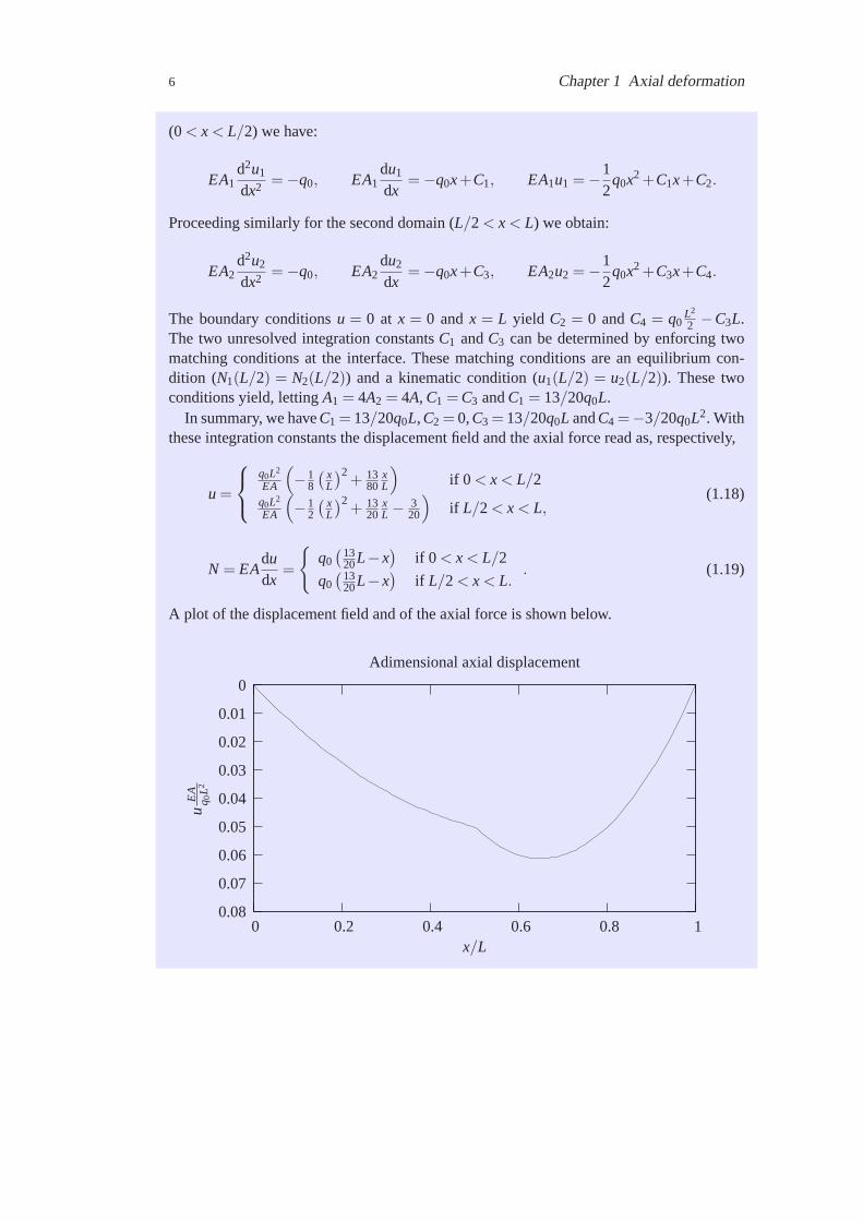
In summary, we haveC1 = 13/20q0L,C2 = 0,C3 = 13/20q0L andC4 =−3/20q0L2. Withthese integration constants the displacement field and the axial force read as, respectively,
u =
q0L2
EA
(
−18
(xL
)2+ 13
80xL
)
if 0 < x < L/2q0L2
EA
(
−12
(xL
)2+ 13
20xL − 3
20
)
if L/2< x < L,(1.18)
N = EAdudx
=
{
q0(
1320L− x
)if 0 < x < L/2
q0(
1320L− x
)if L/2< x < L.
. (1.19)
A plot of the displacement field and of the axial force is shown below.
Adimensional axial displacement
x/L
uE
Aq 0
L2
10.80.60.40.200.08
0.07
0.06
0.05
0.04
0.03
0.02
0.01
0

References 7
Adimensional axial force
x/L
N1 q 0L
10.80.60.40.20
0.6
0.4
0.2
0
-0.2
-0.4
Exercises
1.1 A uniform rod of lengthL is hung vertically under the action of gravity. Show that theloading per unit length isq(x) = ρAg, whereρ is the mass density andg is the gravitationalconstant. Consequently, show that the displacement distribution is
u(x) =ρALEA
gx(
1− x2L
)
.
[Problem 2.1 from Reference [1]]
1.2 Consider a rod of lengthL that has a varying area of the form
A(x) = A1+A21xL
with A21 = A2−A1. If this is fixed at one end and a loadP is applied at the other, show thatthe displacement distribution is
u(x) =PL
EA21ln
[
1+
(A2
A1−1
)xL
]
.
[Problem 2.3 from Reference [1]]
References
[1] J. F. Doyle. Static and Dynamic Analysis of Structures with an Emphasis on Mechanics and ComputerMatrix Methods. Kluwer Academic Publishers, 1991.


Chapter 2
Euler-Bernoulli beam bending
The beam theory presented in this chapter is the results of many years of work by someof the most influential individuals in the mechanics community.This chapter is based on [1, 2, 3, 4].
2.1 Limitations of the theory
The sign conventions employed in this chapter are shown in Figure 2.1. Beamproblems willbe solved with the assumption that the shear strains are approximately zero. This modelis known as technical theory of bending. The technical theory of bending is valid onlyunder the assumption of small displacements. We also assume that the beam hasa straightlongitudinal axis with cross section of any shape provided it is symmetric about they axis.As a consequence of their geometrical proportions, all beams are stable under the actionof the applied load: a thin sheet of paper makes a bad beam as it will buckle sidewise andcollapse.
2.2 Kinematic assumptions
Kinematics describes how the deflection of the beam is tracked. Here, the deflectionv of abeam is defined as the transverse displacement of the center line of the beam in the planexoy. This is the only unknown. The deflection is accompanied by a rotation of the beamneutral plane and by a rotation of the beam cross section.
The key assumption in Euler-Bernoulli beam theory is known as Bernoulli-Navier hy-pothesis:plane cross-sections remain planar and normal to the beam axis in a beam sub-jected to bending. This hypothesis is valid when deformations due to shear and torsion resultsmall compared to those deriving from normal stress and flexural deformation. This hypoth-esis will be somehow relaxed in the Timoshenko beam theory as we shall see inChapter 4.
2.2.1 Relationship between deflection and curvature
Consider Figure 2.2(a). From simple geometric considerations
ds = ρ dθ and κ =1ρ=
dθds
, (2.1)
9

10 Chapter 2 Euler-Bernoulli beam bending
y
xv
+∆θ
+dvdx = θa
b
z
z
y
y
o
+ϕ
x
or
or
=
=+V :
+M:
q
curvature forM > 0
positive curvatured2y
dx2 :
cross section
Figure 2.1 Sign convention in beam problems.
with κ the curvature andρ the radius of curvature. The slope of the deflection curve isevaluated asdv
dx and can be related to the angle of rotation of the axis of the beamθ (seeFigure 2.2(b)) by means of
dvdx
= tanθ . (2.2)
This expression has been obtained by approximating ds with a straight line since dx isinfinitesimal. Note that it is also dx = dscosθ .
Under the assumption of very small rotations, we may set sinθ ≈ tanθ ≈ θ and cosθ ≈ 1.Hence ds = dx, κ = 1
ρ = dθdx and dv
dx = θ . Taking the first derivative ofθ and using theexpression for the curvature we obtain
d2vdx2 = κ =
1ρ. (2.3)
2.2.2 Relationship between curvature and longitudinal str ain
In order to seek the relation between curvature and the associated deformation, we considera portion of beam in pure bending produced by two couplesM0 as shown in Figure 2.3. ThecouplesM0 generate positive curvature and negative bending momentM (negative accordingto our convention stated in Figure 2.1). The beam axis is bent into a circular curve. Indeed,the symmetry of the beam and its loading requires that all elements of the beam deform inan identical manner which is possible only if the deflection curve is circular and if the cross

2.2 Kinematic assumptions 11
x
v
dθ
v+dv
x dx
x
(a)
(b)
y
θ
ρ
O′
dθ
θ
ds
x dx
P
v
ds
Figure 2.2 [1, Figure 7.1]

12 Chapter 2 Euler-Bernoulli beam bending
M0 M0
M0 M0
dθ
x
y
z
y
n q
e fn q
dxm p
pm
O′
y
Figure 2.3 [1, Figure 5.6]
section remain plane during loading. Due to the deformation, the fibers in the upper partof the beam are in tension whereas those in the lower part are in compression. The fiberson the neutral surface of the beam do not change in length. The intersection of the neutralsurface with a cross section is called neutral axis of the cross section. Here, thez axis is theneutral axis for the cross section (this surface is indicated by the dashedline in Figure 2.3).The planes of cross sectionsmn andpq of the deformed beam intersect in a line through thecenter of curvatureO′. The angle between the two planes is denoted by dθ and the distancebetweenO′ and the neutral axis is the radius of curvatureρ.
The initial distance dx between the two planes remains unchanged at the neutral surface.The length dx of a segment on the neutral axis can be related to the radius of curvatureρ bymeans of dx = ρ dθ . On the other hand, a segmente f at distancey from the neutral axis isstrained and its length is now equal to dse f = (ρ − y) dθ . Hence, the strain in the segmente f after bending is equal to
εe fxx =
dse f − dx
dx=−κy. (2.4)
2.3 Relationships between load, shear force and bending mom ent
The relationships between load, shear force and bending moment is derived by expressingthe equilibrium of an infinitesimal element dx of a beam in bending loaded with a dis-tributed load of intensityq as shown in Figure 2.4. The relation between shearing forcesand distributed load is obtained from equilibrium of forces in the vertical direction andreads as
dVdx
=−q. (2.5)

2.4 Relationship between internal bending moment and curvature 13
qdx
M +dMM
V +dVdx
V
y, v
x
Figure 2.4 Element dx of a beam.
The equilibrium equation obtainedby summing moments about an axisthrough the left hand face of the elementand orthogonal to the plane of the figureyields
dMdx
=V, (2.6)
where we have discarded product of dif-ferentials. This equation is valid in re-gions where there is a distributed load.It does not hold where there is a con-
centrated load. A similar set of equation can be derived in case of distributed couples.
2.4 Relationship between internal bending moment and curvat ure
The longitudinal strain (2.4) is related to the stress by means of Hooke’s law through theYoung’s modulus so thatσx = Eεx =−Eκy.
Consider Figure 2.5 representing a portion of a beam in bending where wehave replacedthe internal moment at the right-hand cross section with the corresponding stress distribu-tion. For equilibrium, the internal couple resulting from the sum ofσx dAy over the wholesection must equal the internal momentM. The element of forceσx dA on the element dAacts in the positive direction of thex axis whenσx is positive and in the negative directionwhenσx is negative. Hence, its moment about thez axis is dM =−σxydA. The equilibriumequation obtained by summing moments about thez axis yields
M =
∫
dM =
∫
σxydA, (2.7)
from which, considering the expression of the stressσx
M =
∫
σxydA =−∫
Eκy2dA =−EIκ (2.8)
y y
M Myx
x
σx dAσx
Figure 2.5

14 Chapter 2 Euler-Bernoulli beam bending
where
I =∫
y2dA (2.9)
is the moment of inertia around the neutral axisz (I = Izz andM = Mzz).
2.5 The differential equation of the transverse deflection
The differential equation of the deflection of a beam is obtained by eliminating the curvatureκ from (2.8) and (2.3) to obtain
d2vdx2 =− M
EI. (2.10)
By making use of the relation (2.5) between shearing force and distributed load and (2.6)between shearing force and bending moment, (2.10) can be expressed as
d2
dx2
(
EId2vdx2
)
= q (2.11)
or as
EId4vdx4 = q (2.12)
if the flexural stiffnessEI does not vary withx along the length of the beam.It is worth noticing that the curvature related to a positive bending momentM is opposite
to that related to a positive curvatured2vdx2 of the deflection line. Hence the minus in (2.10).
There is no general consensus on sign convention (cf e.g. [2, 3, 5]). In a system like theone depicted in Figure 2.6(a), the sense of the curvature of the elastic linev and that inducedby a positive bending momentM is the same and the governing differential equation readsas
d2vdx2 =
MEI
(2.13)
whereM =Mzz andI = Izz. On the other hand, the system depicted in Figure 2.6(b) is similarto that reported in Figure 2.1 and the governing differential equation reads as
d2wdx2 =− M
EI(2.14)
whereM = Myy and I = Iyy. The introduction of other sign conventions might seem con-fusing at first. Nevertheless, it is very important to realize that there is morethan one wayof looking at things. After all, quoting Den Hartog [3], the “sign conventionused for shearforce diagrams and bending moments is only important in that it should be used consistentlythroughout a project.”

2.5 The differential equation of the transverse deflection 15
z
y
+q:
+V :
+M:
y
xv
+∆θ+dv
dx = θa
b+V :
+M:
z
xw
+∆θ
+dwdx = θa
b
+q:
curvature forM > 0
curvature forM > 0
curve with 1ρ > 0
curve with 1ρ > 0
(b)
(a)
Figure 2.6 Other sign conventions in beam problems (cf Figure 2.1).
Exercises
2.1
P
A
L L
EI EI
Determine the deflection atA, and show that it can be ob-tained as the sum of the deflection atA of the two beamsbelow. Can this result be generalized to other boundaryconditions and/or other quantities such as rotations andreaction forces? Under what conditions it is valid? Thedeflection atA can be obtained using the second orderdifferential equation function of the bending moment orthe fourth order differential equation function of the dis-
tributed load. Use both differential equations.
P P
A
L L
A
L L
EI → ∞EI EIEI → ∞

16 References
References
[1] J. M. Gere and S. P. Timoshenko.Mechanics of Materials. Wadsworth, Inc., Belmont, California, secondedition, 1984.
[2] E. P. Popov.Introduction to the Mechanics of Solids. Prentice-Hall, Inc., Englewood Cliffs, N.J., 1968.
[3] J. P. Den Hartog.Strength of Materials. Dover Publications, Inc., New York, 1961.
[4] S. P. Timoshenko and D. H. Young.Theory of Structures. McGraw-Hill Book Company, New York, secondedition, 1965.
[5] A. L. Bouma. Mechanica van Constructies. Delftse Uitgevers Maatschappij, Delft, second edition, 1993.

Chapter 3
Deflection of shear beams and frames
According to the Euler-Bernoulli beam theory, cross sections carry a resultant shearingforceV but the deformation associated to the corresponding shear stress is not takeninto account. This anomaly has been resolved by Timoshenko in 1921-22 [1, 2] byapproximating the effect of shear as an average over the cross section– in reality, theshear stress and strain vary over the cross section. An extension of theEuler-Bernoullibeam theory that includes transverse shear deformation is discusses in Chapter 4.In this chapter, we shall concentrate on the ideal shear beam employing a constantshear stress over a cross section. This kind of beam exhibits no flexural deformationbut deforms in shear only. However, the beam is subjected to bending moments even ifthese moments do not contribute to the deformation.
3.1 The governing equation
dxdx
γdv
qdx
V V + dV
y
x
z
Figure 3.1
The kinematic quantity describing sheardeformation is the shear distortionγcaused by the shear forceV as shown inFigure 3.1. The shear distortion is related,in small deformation, to the deflectionvby means of the kinematic relationship
γ ≈ dvdx
(3.1)
which can be derived with simple ge-ometrical considerations analyzing Fig-ure 3.1. Assuming a linear elastic mate-rial, the constitutive equation is formu-lated in terms of Hooke’s law by speci-fying the relationship
τ = Gγ (3.2)
between the deformation, i.e. the shear strainγ, and the stress, i.e. the shear stressτ. Con-sidering an average expression of the shear forceτ acting on a section,
τ =VAs
(3.3)
17
18 Chapter 3 Deflection of shear beams and frames
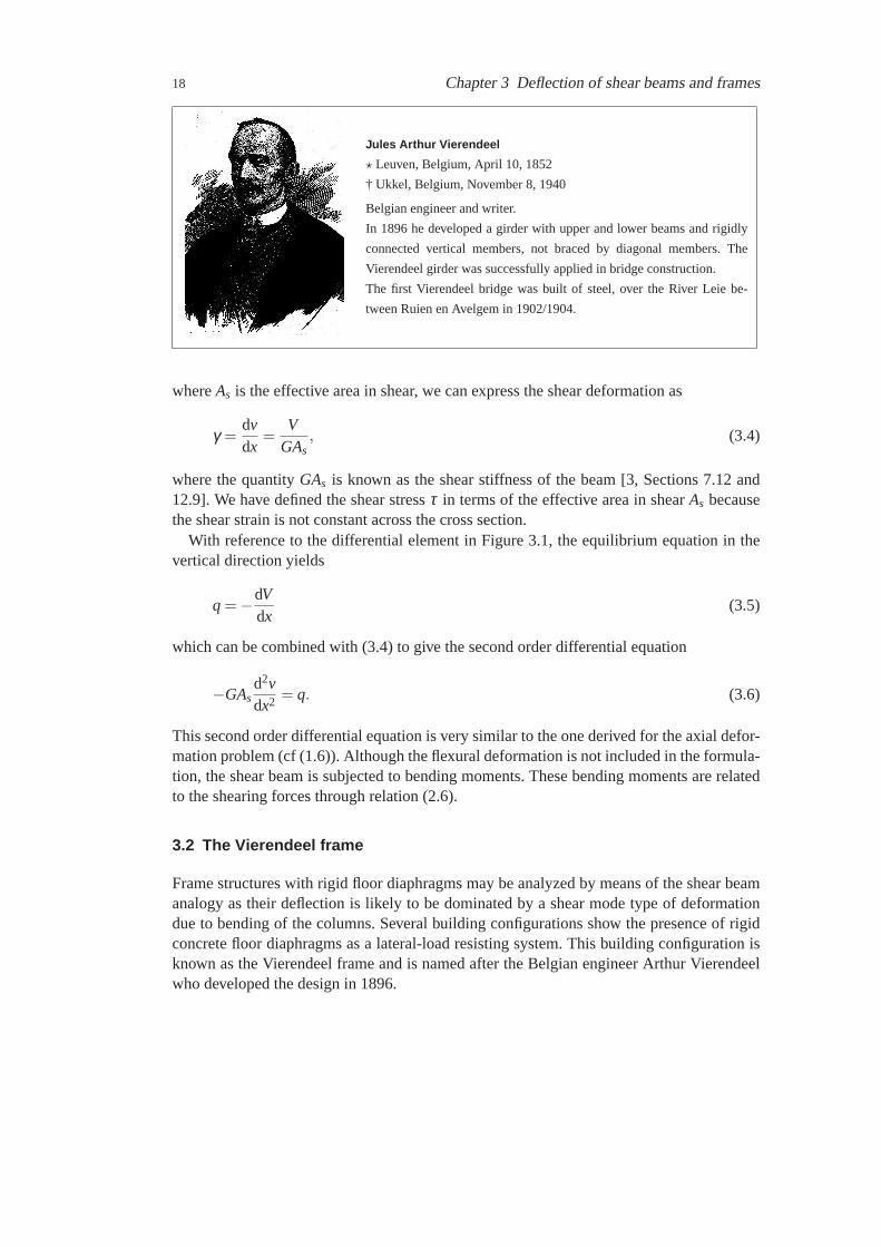
Jules Arthur Vierendeel
⋆ Leuven, Belgium, April 10, 1852
† Ukkel, Belgium, November 8, 1940
Belgian engineer and writer.
In 1896 he developed a girder with upper and lower beams and rigidly
connected vertical members, not braced by diagonal members. The
Vierendeel girder was successfully applied in bridge construction.
The first Vierendeel bridge was built of steel, over the River Leie be-
tween Ruien en Avelgem in 1902/1904.
whereAs is the effective area in shear, we can express the shear deformation as
γ =dvdx
=V
GAs, (3.4)
where the quantityGAs is known as the shear stiffness of the beam [3, Sections 7.12 and12.9]. We have defined the shear stressτ in terms of the effective area in shearAs becausethe shear strain is not constant across the cross section.
With reference to the differential element in Figure 3.1, the equilibrium equation in thevertical direction yields
q =−dVdx
(3.5)
which can be combined with (3.4) to give the second order differential equation
−GAsd2vdx2 = q. (3.6)
This second order differential equation is very similar to the one derived for the axial defor-mation problem (cf (1.6)). Although the flexural deformation is not includedin the formula-tion, the shear beam is subjected to bending moments. These bending moments are relatedto the shearing forces through relation (2.6).
3.2 The Vierendeel frame
Frame structures with rigid floor diaphragms may be analyzed by means of the shear beamanalogy as their deflection is likely to be dominated by a shear mode type of deformationdue to bending of the columns. Several building configurations show the presence of rigidconcrete floor diaphragms as a lateral-load resisting system. This building configuration isknown as the Vierendeel frame and is named after the Belgian engineer Arthur Vierendeelwho developed the design in 1896.

3.2 The Vierendeel frame 19
The Vierendeel frame, sometimes referred to as Vierendeel truss or Vierendeel beam,was initially employed in some bridges like the ones shown in Figures 3.2 and 3.3. Thisframe is nowadays rarely used in bridges owing to a lesser economy of materials whencompared to other solutions. Although the Vierendeel frame is not an efficient means oftransmitting transverse load, it is however used to resist lateral load in buildings. It is alsopopular in the design of unconventional buildings for architectural reasons–the headquartersof the Commerzbank in Frankfurt, shown in Figure 3.4, and the Beinecke Rare Books &Manuscripts Library, Yale, shown in Figure 3.5, are typical examples.
This system is characterized by rigid joints, upper and lower beams and is a staticallyindeterminate truss in which all members are subject to bending moments.
3.2.1 Commerzbank headquarters
The building of the Commerzbank headquarters was designed by Norman Foster and engi-neered by Ove Arup. With a structural height of 259 m, the Commerzbank Tower, built in1997, was the tallest building in Europe until the completion in December 20, 2003, of theTriumph Palace, an apartment building in Moscow.
Floors between sky gardens are supported by eight-story high Vierendeel frames whichalso resist lateral load. Pairs of vertical masts, enclosing the corner cores, support eight-storyVierendeel trusses, which in turn support clear-span office floors.There are no columnswithin the offices and the Vierendeel frames enable the gardens to be totally free of structure.
3.2.2 Beinecke Rare Books & Manuscripts Library
The Beinecke Rare Books & Manuscripts Library is located on the campus of Yale Univer-sity in New Haven, Connecticut. The library opened in 1963 and is a big box of translucentmarble on little feet. It was designed by Gordon Bunshaft, of the famous NewYork Cityarchitectural firm of Skidmore, Owings and Merrill.
The library features five-story Vierendeel frames supported by fourconcrete cornercolumns. Facades are assembled from prefab steel crosses welded together at inflectionpoints.
Figure 3.2 The first Vierendeel bridge was built in steel over the River Leie (1902/1904).The photos show different stages of construction. The span of the bridge was 42 m.

20 Chapter 3 Deflection of shear beams and frames
Figure 3.3 The Lanaye bridge in Belgium (1932) was blown up by the Belgian Army asa precaution measure to obstruct the German troops on May 11, 1940, oneday after theGerman invasion of Belgium. The span of the bridge was 88 m.
Example 3.1 A multi-story building with rigid floor diaphrag ms as a shear beam
Consider a two-dimensional schematic of a multi-story building with rigid floor diaphragmsdepicted in the left part of the figure below (this system is known as “rigid jointed unbracedframe” or Vierendeel frame). Since the load is transmitted unaltered from floor to floor, it ispossible to study the whole building by analyzing the single bay equivalent (shown in theright part of the figure).
Figure 3.4 Commerzbank headquarters in Frankfurt Am Main.

3.2 The Vierendeel frame 21
Figure 3.5 Beinecke Rare Books & Manuscripts Library. Length direction span: 131 feet(≈ 40 m) – Width direction span: 80 feet (≈ 25 m).
H
h
∆v
EI = ∞
EI = ∞
EIEI
(b)
γ
(a)
x
H
y, v
From simple considerations, the deflection∆v of the single story due to a horizontal forceH is equal to
∆v =Hh3
24EI, (3.7)
where we have considered that the forceH is equally distributed between the two columns.Under the assumption of small deflections, (3.7) can be re-written as
H =24EI
h2
∆vh
=24EI
h2 γ = kγ (3.8)

22 Chapter 3 Deflection of shear beams and frames
which is similar to the constitutive equation of a shear beam wherek is the shear stiffnessof the portal (cf (3.2)).
Since the force transmitted to each floor is the same, this result is valid for all floors. As aconsequence, all joints of the columns will remain on a straight line after shear deformation,similar to the deformation of a shear beam. Indeed, with top point load, the internal shearingforce anddv
dx are constant and the deflected shape is a straight line. Thus the deflectionof a Vierendeel frame can be estimated using the shear beam deflection formula with theequivalent shear stiffnessk from (3.8). The situation is however different in the case of auniformly distributed load as shown in the next example.
Example 3.2 A shear frame with a distributed lateral loadWhen a distributed lateral load is applied to a shear frame, the deflection is parabolic.Consider the frame depicted below. Equation (3.5) is integrated once to obtain
F F
x
q0
y, v
L
b
V =−q0x+C1
(
= GAsdvdx
)
. (3.9)
A second integration (or integration of (3.6)) yields
GAsv =−12
q0x2+C1x+C2, (3.10)
whereC1 andC2 are integration constants that can bedefined by means of the boundary conditionsv = 0 atx = 0 andV = 0 atx = L. With these boundary condi-tionsC1 = q0L andC2 = 0. Hence
V = q0(L− x) (3.11)
and
GAsv =12
q0x(2L− x) . (3.12)
Extreme values arev = 0 andV = q0L at x = 0 andv = q0L2/2GAs andV = 0 atx = L.
In addition to the horizontal reaction forceV = q0L, the supports provide vertical reactionforcesF . These reaction forces acting at distanceb can be found by rotational equilibriumat one of the supports (F = q0L2/2b).
The internal bending momentM can be derived through integration of (2.6) withM = 0at x = L as boundary condition. A simple calculation yields
M = q0x(
L− x2
)
− 12
q0L2. (3.13)

References 23
Exercises
3.1 Compare the deflected shape and the shear force diagram of the two beamsbelow con-sidering the shear beam theory and the Euler-Bernoulli beam theory. Discuss the influenceof the linear spring and its position.
p
L−a a
ks
L−a a
q
ks
3.2 Determine the expression of the deflected shape and the shear force diagram of thebeams below and sketch them. All the beams have shear stiffnessk.
p
L/2 L/2
q
L/2 L/2
L/2 L/2
q
L/2 L/2
q
References
[1] S. P. Timoshenko. On the correction for shear of the differential equation for transverse vibrations ofprismatic bars.Philosophical Magazine, 41:744–746, 1921.
[2] S. P. Timoshenko. On the transverse vibrations of bars of uniformcross-section.Philosophical Magazine,43:125–131, 1922.
[3] J. M. Gere and S. P. Timoshenko.Mechanics of Materials. Wadsworth, Inc., Belmont, California, secondedition, 1984.


Chapter 4
Timoshenko beam theory
The Timoshenko beam theory [1, 2] is an extension of the Euler-Bernoullibeam the-ory that includes first-order transverse shear effect. The core assumption of the Euler-Bernoulli beam theory, i.e. plane cross sections perpendicular to the beam axis remainplane and perpendicular to the neutral axis during bending, is relaxed. This relaxationis introduced through an additional degree of freedom which describesthe additionalrotation to the bending slope. This extra rotation generates a shear strain. This beammodel was presented in 1922 in the context of vibration and dynamics. Similar totheshear beam described in Section 3, a constant shear over the beam height is assumed.
4.1 Kinematic assumptions
The relaxation of the normality assumption of plane sections that remain plane and normalto the deformed centerline is what distinguishes the Timoshenko beam theory from theEuler-Bernoulli beam theory. In the Timoshenko beam theory there are two independentkinematic quantities: the transverse deflectionv(x) and the cross sectional rotationϕ (x) –ϕ is the rotation of the cross section with respect to the vertical axis or, equivalently, therotation angle of the generic cross section with respect to his tangent.
Consider Figure 4.1. The displacement field for a pointp at distancey from the center of
Stepan Prokofyevich Timoshenko
⋆ Shpotivka in Poltava Gubernia, Russia (now in Chernihiv Oblast,
Ukraine), December 23, 1878
† Wuppertal, Germany, May 29, 1972
He is reputed to be the father of modern engineering mechanics. He
wrote many of the seminal works in the areas of engineering mechan-
ics, elasticity and strength of materials, many of which are still widely
used today.
In 1957 the American Society of Mechanical Engineers established the
Timoshenko Medal in his honor, and he was the first recipient of this
annual award because “by his invaluable contributions and personal ex-
ample, he guided a new era in applied mechanics.”
25

26 Chapter 4 Timoshenko beam theory
y
x
y
z
vsy
ϕ
a′
a
b
psx y
b′
Figure 4.1
the beam on the cross sectionab is described by
sx (x,y) =−yϕ (x) and sy (x,y) = v(x) . (4.1)
From the displacement field we derive the non-zero components of the strain field as
εx =dsx
dx=−y
dϕdx
and γxy =dsx
dy+
dsy
dx=−ϕ +
dvdx
. (4.2)
4.2 Relationships between deformations and internal forces
The shear deformationγ is related to the shear force through (3.4). By making use of (4.2)2
we obtain the following expression for the shear force:
V = GAsγ = GAs
(dvdx
−ϕ)
. (4.3)
From Hooke’s law and making use of (4.2)1:
σx = Eεx =−Eydϕdx
. (4.4)
By making use of the above expression for the longitudinal stress and following consid-erations similar to those reported in Section 2.4, the bending momentM is expressed as afunction of the cross sectional rotationϕ according to
M =−EIdϕdx
. (4.5)

4.3 Limit cases 27
4.3 Limit cases
The shear beam and the classical beam theories are recovered by an appropriate choice ofthe flexural stiffnessEI and the shear stiffnessGAs. The Euler-Bernoulli beam is recoveredwhenGAs → ∞. In this case there is no shear andγ → 0. This implies thatdv
dx → ϕ and
M →−EI d2vdx2 . WhenEI → ∞ there is no bending (ϕ = 0) and the shear beam is recovered.
Only the shear deformation is present. In this caseγ → dvdx andq =−dV
dx →−GAsd2vdx2 .
4.4 The differential equations governing the transverse deflec tion and crosssectional rotation
The equilibrium of an infinitesimal beam segment is not affected by the addedshear de-formation. As a consequence, the relationships derived in Section 2.3 arestill valid. Inparticular, we derive the differential equations governing the transverse deflection and crosssectional rotation of the Timoshenko beam by eliminating the shear forceV and the bendingmomentM from (2.5) and (2.6).
Let us use the equilibrium relation (2.6). We considerV from (4.3) and express the firstderivative ofM from (4.5). Substituting these expressions ofV andM into (2.6) yields
EId2ϕdx2 +GAs
(dvdx
−ϕ)
= 0. (4.6)
We now make use of the second equilibrium relation (2.5). As before, we considerVfrom (4.3) and replace its derivative in (2.5) to obtain
GAs
(d2vdx2 −
dϕdx
)
=−q. (4.7)
Equations (4.7) and (4.7) are two coupled second order differential equations governing thedeflectionv and the cross sectional rotationϕ of the Timoshenko beam. The problem isfully determined with the definition of four boundary conditions.
Example 4.1
P
y, v
x
L
a
Consider a cantilever beam with a concen-trated loadP at the free end. In this case thereis no distributed load and the governing equa-tion (4.7) simplifies to
d2vdx2 =
dϕdx
. (4.8)
Differentiating (4.6) once and combining itwith (4.8) yields
EId4vdx4 = 0. (4.9)

28 Chapter 4 Timoshenko beam theory
The differential equations (4.8) and (4.9) are the governing equations for the cantileverbeam without distributed load. It is interesting to notice that (4.9) is the ordinary beamtheory equation.
Direct integration of (4.9) yields:
EIv =C1x3
6+C2
x2
2+C3x+C4. (4.10)
The problem is completely specified by the following boundary conditions: 1)M = 0 atx = 0; 2)V =−P atx = 0; 3)ϕ = 0 atx = L; 4) v = 0 atx = L. Application of the boundaryconditions results in the following:
bc 1) M = 0 atx = 0 implies dϕdx = 0. By making use of (4.8) we haveC2 = 0;
bc 2) V = −P at x = 0: we make use of (2.6) from whichV = −EI d3vdx3 . The boundary
condition impliesC1 = P;
bc 3) ϕ = 0 atx = L: using (4.3) withV =−P at x = L impliesC3 =−PEIGAs
− PL2
2 ;
bc 4) v = 0 atx = L impliesC4 =PLEIGAs
+ PL3
3 .
With these integration constants, the deflection reads
v =Px3
6EI− PL2x
2EI+
PL3
3EI︸ ︷︷ ︸
bending
+P
GAs(L− x)
︸ ︷︷ ︸
shear
(4.11)
while the deflection at the free end is
va =PL3
3EI+
PLGAs
=PL3
3EI
(
1+3EI
GAsL2
)
. (4.12)
The relative importance of the shear contribution can be appreciated by analyzing the lastterm in this equation. Usually, for very slender beams, the shear component can be ne-glected. However, for span/cross section heightL/h such that the beam can be consideredthick, the shear contribution becomes important.
Exercises
4.1 A Timoshenko beam is clamped at the two ends. A prescribed transverse deflection uis applied at one of the two ends. Compute the expression of the deflected shape and ofthe shearing force and bending moment diagrams and sketch them. Expressthe value ofthe reaction forces and moments at the two ends as a function of the parameterΦ = 12EI
GAsL2 .Show that the shear beam and the Euler-Bernoulli beam results are recovered as limit cases(express the limit cases as function ofΦ).

References 29
4.2 Compare the influence of the shear contribution in the above exercise and inExam-ple 4.1. What are the factors that contribute the most? What is the role of the boundaryconditions?
References
[1] S. P. Timoshenko. On the correction for shear of the differential equation for transverse vibrations ofprismatic bars.Philosophical Magazine, 41:744–746, 1921.
[2] S. P. Timoshenko. On the transverse vibrations of bars of uniformcross-section.Philosophical Magazine,43:125–131, 1922.


Chapter 5
Beams and frames on elastic foundation
In this chapter we shall study the behavior of beams and shear frames on elastic founda-tion. The foundation or soil can be replaced by a set of distributed linear elastic springs.Similar to the pull-out problem described in Section 1.5, we consider the forcerelatedto these spring to be proportional and opposite to the displacement. Sign conventionfollows those used in Chapters 2 and 3.This chapter is based on [1]. A review of possible approaches to the study of beams onelastic foundation can be found in [2].
5.1 The differential equation of the elastic line
(q− kv) dx
M +dMM
V +dVdx
V
y, v
x
Figure 5.1
The only difference with the Euler-Bernoulli beam and the shear beam is thepresence of a distributed load proportionalto the displacement. Hence, we can startthe derivation of the differential equationof the elastic line by considering the equi-librium of a differential element. With ref-erence to Figure 5.1, equilibrium of forcesin the vertical direction yields
dVdx
− kv =−q, (5.1)
wherek is the soil stiffness. The equilib-rium equation obtained by summing moments about an axis through the left hand face ofthe element and orthogonal to the plane of the figure yields the same equation as (2.6).
5.1.1 The shear beam
With trivial manipulations, the differential equation of the deflection of a shear beam(cf (3.6)) can be expressed as
−GAsd2vs
dx2 + kv = q. (5.2)
31

32 Chapter 5 Beams and frames on elastic foundation
It is convenient to consider the following form of the homogeneous equation
d2vs
dx2 −α2v = 0 (5.3)
with α2 = kGAs
. This equation is identical to (1.13)2 and we refer to Section 1.5 for itssolution.
Particular solutions
Particular solutions account for the non-homogeneous term in (5.1). Forthe shear beam,some particular solutionsv(x) are as follows.
Uniform distributed loadq(x) = q0 : v(x) = q0k
Loadq(x) = q0x : v(x) = q0k x
Sinusoidal loadq(x) = q0sinπxl : v(x) = q0
GAs( πL )
2+k
sinπxL
5.1.2 The Euler-Bernoulli beam
The differential equation of the deflection curve of a Euler-Bernoulli beam supported on anelastic foundation can be derived using (5.1) and following the line of reasoning reported inChapter 2. With some simple manipulation we obtain
EId4vdx4 + kv = q. (5.4)
The homogeneous counterpart of (5.4) can be written as
d4vdx4 +
kEI
v = 0. (5.5)
Substitutingv = emx in (5.5) we obtain the characteristic equation
m4+k
EI= 0 (5.6)
which has the roots
m1 =−m3 = λ (1+ i) , m2 =−m4 = λ (−1+ i) , (5.7)
with λ 4 = k/4EI. The general solution of (5.5) is then
v =1,4∑
i
Aiemix (5.8)
which can be written in a more convenient form using
eiλx = cosλx+ isinλx, e−iλx = cosλx− isinλx (5.9)
5.2 Examples 33
as
v = eλx (C1cosλx+C2sinλx)+e−λx (C3cosλx+C4sinλx) . (5.10)
The new integration constantsC1, C2, C3 andC4 are related to the old ones through
C1 = A1+A4, C2 = i(A1−A4) , C3 = A2+A3, C4 = i(A2−A3) . (5.11)
The factorλ is called thecharacteristics of the system and has dimensions of length−1. Theterm 1/λ is referred to as thecharacteristic length.
Equation (5.10) is the general solution for the deflection line of a straight prismatic Euler-Bernoulli beam supported on an elastic foundation under the action of transverse bendingforces. An additional term is necessary if a distributed loadq is present. The slope, thebending moment and the shearing force can be obtained by the relationshipsderived inChapter 2.
The four integration constantsC1, C2, C3 andC4 can be determined from conditions onthe deflectionv, the slopeθ , the bending momentM or the shearing forceV existing at thetwo ends of the beam.
Particular solutions
Particular solutions account for the non-homogeneous term in (5.4). Forthe Euler-Bernoullibeam, some particular solutionsv(x) are as follows.
Uniform distributed loadq(x) = q0 : v(x) = q0k
Loadq(x) =max 3∑
i=0aixi : v(x) = q(x)
k
Sinusoidal loadq(x) = q0sinπxL : v(x) = q0
π4 EIL4+k
sinπxL
5.2 Examples
The solutions derived above, with the proper boundary conditions, canbe used to solve awide variety of problems. Below we illustrate some typical examples.
An interesting property of the solution of this class of problem lies in the fact that theprinciple of superposition can be applied without restrictions to all quantities of interest.Indeed, the deflection, the slope, the bending moment and the shearing force are directlyproportional to the load.
Example 5.1 (Beam of infinite length subjected to a concentra ted force)Consider a beam of infinite length subjected to a concentrated force. We can assume thatthe transverse deflection is zero at infinite distance from the application of the load. Thiscondition implies that the term connected to eλx in (5.10) vanishes and
v = e−λx (C3cosλx+C4sinλx) . (5.12)
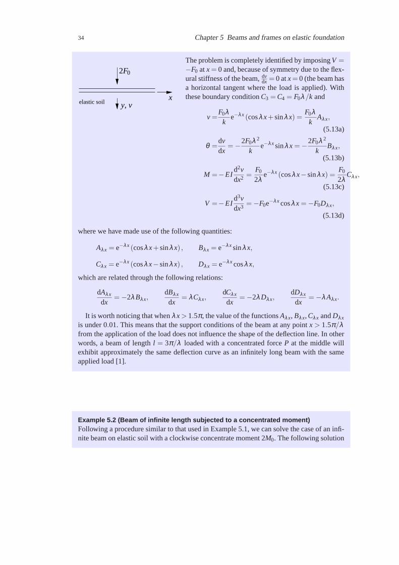
34 Chapter 5 Beams and frames on elastic foundation
elastic soilx
2F0
y, v
The problem is completely identified by imposingV =−F0 atx = 0 and, because of symmetry due to the flex-ural stiffness of the beam,dv
dx = 0 atx= 0 (the beam hasa horizontal tangent where the load is applied). Withthese boundary conditionC3 =C4 = F0λ/k and
v =F0λ
ke−λx (cosλx+sinλx) =
F0λk
Aλx,
(5.13a)
θ =dvdx
=−2F0λ 2
ke−λx sinλx =−2F0λ 2
kBλx,
(5.13b)
M =−EId2vdx2 =
F0
2λe−λx (cosλx−sinλx) =
F0
2λCλx,
(5.13c)
V =−EId3vdx3 =−F0e−λx cosλx =−F0Dλx,
(5.13d)
where we have made use of the following quantities:
Aλx = e−λx (cosλx+sinλx) , Bλx = e−λx sinλx,
Cλx = e−λx (cosλx−sinλx) , Dλx = e−λx cosλx,
which are related through the following relations:
dAλx
dx=−2λBλx,
dBλx
dx= λCλx,
dCλx
dx=−2λDλx,
dDλx
dx=−λAλx.
It is worth noticing that whenλx > 1.5π, the value of the functionsAλx, Bλx,Cλx andDλx
is under 0.01. This means that the support conditions of the beam at any pointx > 1.5π/λfrom the application of the load does not influence the shape of the deflection line. In otherwords, a beam of lengthl = 3π/λ loaded with a concentrated forceP at the middle willexhibit approximately the same deflection curve as an infinitely long beam with thesameapplied load [1].
Example 5.2 (Beam of infinite length subjected to a concentra ted moment)Following a procedure similar to that used in Example 5.1, we can solve the caseof an infi-nite beam on elastic soil with a clockwise concentrate moment 2M0. The following solution

5.2 Examples 35
is valid for x > 0:
v =2M0λ 2
kBλx, (5.14a)
θ =dvdx
=2M0λ 3
kCλx, (5.14b)
M =−EId2vdx2 = M0Dλx, (5.14c)
V =−EId3vdx3 =−M0λAλx. (5.14d)
For those points on the left of the point of application of the moment, the sign ofv andMmust be reversed. Note that the arguments of the functionsAλx, Bλx, Cλx andDλx are alwaystaken as positive, irrespective of the location ofx with respect to the point of application ofthe moment.
Example 5.3 (How to speed-up derivations)Considering again the beam of infinite length subjected to a concentrated force in Exam-ple 5.1, we can express (5.13) in a format that allows a quick computation of the variousderivatives involved. To this end, we set the integration constants in (5.12) as
C3 = Asinω and C4 = Acosω (5.15)
with which we have
v = e−λx (Asinω cosλx+Acosω sinλx) = Ae−λx sin(λx+ω) . (5.16)
This is the expression of a sinusoidal curve with decreasing amplitudeAe−λx, angular fre-quencyλ and phase angleω . Its derivative is equal to
dvdx
=−λAe−λx sin(λx+ω)+λAe−λx cos(λx+ω) , (5.17)
which can be expressed as
dvdx
=−λ√
2Ae−λx sin(
λx+ω − π4
)
(5.18)
if we multiply the first terms by√
2cosπ/4(= 1) and the second by√
2sinπ/4(= 1). Itis worth noticing that the differentiation implied the multiplication of the amplitude by thefactor−λ
√2 and a phase decrease ofπ/4. Hence
M =−EId2vdx2 =−2λ 2EIAe−λx sin
(
λx+ω − π2
)
, (5.19)

36 Chapter 5 Beams and frames on elastic foundation
and
V =−EId3vdx3 = 2
√2λ 3EIAe−λx sin
(
λx+ω − 3π4
)
. (5.20)
The constantsA andω are found with the boundary conditions atx = 0. From the con-dition on the slope we find thatω = π/4 and from the condition on the shearing forceA = F0λ
√2/k. Hence
v =F0λ
√2
ke−λx sin
(
λx+π4
)
, (5.21a)
θ =dvdx
=−2F0λ 2
ke−λx sinλx, (5.21b)
M =−EId2vdx2 =− F0√
2λe−λx sin
(
λx− π4
)
, (5.21c)
V =−EId3vdx3 = F0e−λx sin
(
λx− π2
)
. (5.21d)
Example 5.4 (Beam of semi-infinite length)
elastic soilx
F0
M0
y, v
Consider a semi-infinite beam on elastic foundationunder the action of two concentrated loads, force andbending moment. Equation (5.10) is the general so-lution for the deflection of an Euler-Bernoulli beamon elastic foundation. Sincew(x)→ 0 for x → ∞, wemust haveC1 = C2 = 0. The boundary conditions atx = 0 determineC3 andC4:
M (0) =−EId2vdx2 (0) = M0 →C4 =
2λ 2M0
k,
V (0) =−EId3vdx3 (0) =−F0 →C3 =
2λF0
k− 2λ 2M0
k.
Armed with these expressions we find
w(x) =2λF0
kDλx −
2λ 2M0
kCλx,
dvdx
(x) =−2λ 2F0
kAλx +
4λ 3M0
kDλx,
M (x) =−EId2vdx2 (x) =−F0
λBλx +M0Aλx,

5.2 Examples 37
and
V (x) =−EId3vdx3 (x) =−F0Cλx −2M0λBλx.
Example 5.5 (An application of the principle of superpositi on)
elastic soilelastic soilx x
y, v
F02
M0
(b)y, v
F0
(a)
By using the expressions derived in Example 5.4, we can determine the solution for a beamof infinite length on elastic foundation under the action of a concentrated force.
Indeed, the beam on the left-hand side of the figure can be equivalent tothe beam depictedin the lower part. The difference between these two cases lies in the slopedv
dx at the point ofapplication of the force which, for the beam on the left-hand side of the figure is zero. Wecan make use of this fact to derive a boundary condition atx = 0 for the beam in the upperpart. Atx = 0 the slope derived in the previous example is
dvdx
=−2λ 2 F02
k+
4λ 3M0
k,
where we have used a load of intensityF0/2. By setting the slope to zero, we can derivethe value of the bending moment that neutralize the slope created by the concentrated force.Proceeding along this line, we obtain
M0 =F0
4λ.
Finally, using the expressions from the previous example withF0/2 andM0 = F0/4λ , weobtain the solution for the beam of infinite length:
w(x) =λF0
2kAλx,
dvdx
(x) =−λ 2F0
kBλx,
M (x) =−EId2vdx2 (x) =
F0
4λCλx,
38 Chapter 5 Beams and frames on elastic foundation
V (x) =−EId3vdx3 (x) =−F0
2Dλx,
which can be compared to the expressions reported in (5.13). These expressions are validfor x > 0. The expressions forx < 0 are obtained from the symmetry and antisymmetryconditions:w(x) = w(−x), dv
dx (x) =−dvdx (−x), M (x) = M (−x), V (x) =−V (−x).
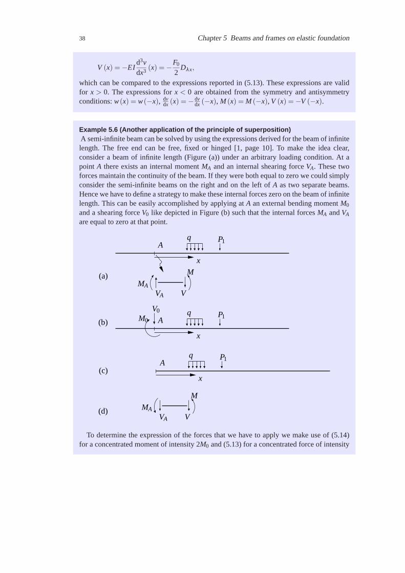
Example 5.6 (Another application of the principle of superp osition)A semi-infinite beam can be solved by using the expressions derived for the beam of infinitelength. The free end can be free, fixed or hinged [1, page 10]. To make the idea clear,consider a beam of infinite length (Figure (a)) under an arbitrary loadingcondition. At apoint A there exists an internal momentMA and an internal shearing forceVA. These twoforces maintain the continuity of the beam. If they were both equal to zero we could simplyconsider the semi-infinite beams on the right and on the left ofA as two separate beams.Hence we have to define a strategy to make these internal forces zero on the beam of infinitelength. This can be easily accomplished by applying atA an external bending momentM0
and a shearing forceV0 like depicted in Figure (b) such that the internal forcesMA andVA
are equal to zero at that point.
q P1A
x
(b) M0
V0
q P1A
x
MAVA
M
V
(a)
q P1A
x(c)
(d) MAVA
M
V
To determine the expression of the forces that we have to apply we make useof (5.14)for a concentrated moment of intensity 2M0 and (5.13) for a concentrated force of intensity

5.2 Examples 39
2V0. We then know that a moment of intensityM0 will produceM = M0Dλx/2 andV =−M0λAλx/2, and a forceV0 will produceM =V0Cλx/4λ andV =−V0Dλx/2. Our objectiveis to let these external force and moment generate internal forces opposite and equal toMA
andVA. Therefore, the equilibrium condition that needs to be fulfilled is like that depictedin Figure (d) which, in combination with the above expressions for internal shearing forceand bending moment, gives
M0
2+
V0
4λ+MA = 0 and VA −
V0
2− M0λ
2= 0, (5.22)
from which
M0 =−4
(
MA +VA
2λ
)
and V0 = 4(λMA +VA) . (5.23)
We may say thatV0 andM0 in (5.23) are such that the beam in Figure (b) and Figure (c) areidentical forx > 0. We callV0 andM0 the end-conditioning forces.
Example 5.7 (Semi-infinite beam with a concentrated load)
F0A
elastic soil
Consider the semi-infinite beam witha concentrated load at the free endshown beside. The boundary conditionsat pointA areM = 0 andV = −F0. Bymaking use of the scheme depicted inFigure (d) of Example 5.6, we found
that MA = 0 andVA = F0. Substituting these values into (5.23) we obtain the correspond-ing end-conditioning forcesV0 = 4F0 andM0 = −2F0/λ . If we apply these forces on theinfinite beam, using (5.14) for the concentrated moment of intensityM0 and (5.13) for aconcentrated force of intensityV0, we obtain the solution forx > 0:
v =2F0λ
kDλx, (5.24a)
θ =− 2F0λ 2
kAλx, (5.24b)
M =−EId2vdx2 =−F0
λBλx, (5.24c)
V =−EId3vdx3 =−F0Cλx. (5.24d)
The same results could have been obtained by directly integrating (5.10) with the boundaryconditionsv = 0 for x → ∞ (C1 = C2 = 0) andM = 0, V = −F0 at x = 0 (C4 = 0, C3 =2F0λ/k). Compare these results with those obtained in Example 5.4 by lettingM0 = 0.

40 Chapter 5 Beams and frames on elastic foundation
Example 5.8 (Beam of finite length)
elastic soil
F0
y, v
A
x
Consider a beam of finite lengthl on elas-tic foundation under the action of a concen-trated loadF0. We would like to determinethe length of the beam so that the deflectionv(x) derived for a beam of infinite length canbe used with confidence in this case.
The deflectionv(x) can be expressed by
v =F0λ2k
e−λx (cosλx+sinλx) =F0λ2k
Aλx,
with the functionAλx shown in the figure below.
βx
Aβ
x
3π5π22π3π
2ππ20
1
0.8
0.6
0.4
0.2
0
-0.2
The length of the beam can be determined by evaluating the functionAλx at a few pointsas shown below.
λx Aλx |Aλx| [%]0 +0.10000E +01 100.000π2 +0.20788E +00 20.788π −0.43214E −01 4.3213π2 −0.89833E −02 0.898
2π +0.18674E −02 0.1875π2 +0.38820E −03 0.039
3π −0.80700E −04 0.008
Whenλx > 3π2 , |Aλx|< 1%. This means that for points at a distance larger than3
2πλ from the

5.3 Classification of beams according to stiffness 41
point of application of the concentrated force, the effect of the soil stiffness on the deflectioncan be neglected. Therefore, a beam of lengthl > 23
2πλ with a concentrated load applied at
midspan exhibits approximately the same deflection curve as an infinitely long beam underthe action of a concentrated load of the same intensity.
Example 5.9 (A shear beam of infinite length on an elastic foun dation)
∞ ∞
2F F
y(a) (b)
x
Consider a shear beam of infinite length on an elastic foundation subjected toa concentratedforce. We make use of symmetry and study only half of the beam with half of theload. Thegoverning equation is (5.3) which is analogous to the equation for the axial deformationproblem that we have studied in Section 1.5. Hence
v =F
GAsαe−αx and V =−Fe−αx. (5.25)
In deriving these expressions, we have considered the following boundary conditions:v = 0for x →∞ andV =−F atx = 0. These expressions are valid forx > 0. Because of symmetryconditions, the displacement function is an even function (it it the same on bothsides of thevertical axis) which impliesv(x) = v(−x). On the other hand, the shear, being the derivativeof the displacement field according toV = GAs
dvdx is an odd function which implies that
V (x) =−V (−x).
5.3 Classification of beams according to stiffness
This section is based on [1, Section 17]. The quantityλ l characterizes the relative stiffnessof a beam on an elastic foundation. This quantity determines the magnitude of thecurvatureof the elastic line and defines the rate at which the effect of a loading forcedies out in theform of a damped wave along the length of the beam. According to theseλ l values we mayclassify beams in three groups:
I Short beams (λ l < π/4): we can neglect the bending deformation of the beam as it issmall compared with the deformation produced in the foundation. Hence, beams withλ l < π/4 can be considered rigid;
II Beams of medium length (π/4 < λ l < π): we need to do accurate computation of

42 References
the beam. These beams are such that a force acting at one end has a finite and notnegligible effect at the other end;
III Long beams (λ l > π): These beams are such that a force acting at one end has anegligible effect at the other end. This means thatλ l is so large that we can take inall the formulasAλ l = Bλ l =Cλ l = Dλ l = 0.
The classification is made from a practical point of view since it offers the possibility of us-ing simplifications by neglecting certain quantities in particular instances. Of course, theselimits depend on the accuracy required in the computations.
Exercises
5.1 Determine the deflection and bending moment atx = l/2. Discuss the role ofλ l.
q(x) = q0sinπxl
kl
EI
x
5.2
References
[1] M. Hetenyi. Beams on elastic foundation. The University of Michigan Press, eight edition, 1967.
[2] Y. H. Wang, L. G. Tham, and Y. K. Cheung. Beams and plates on elastic foundations: A review.Progressin Structural Engineering and Materials, 7(4):174–182, 2005.

Chapter 6
Transverse deflection of cables
Flexible cables are used in suspension bridges, transmission lines, lifts and inmanyother structures. In the design of these structures it is necessary to know the relationbetween cable sag, tension and span – cable sag is defined as the maximum verticaldisplacement of the cable. We shall determine these quantities by examining the cableas a body in equilibrium. In the analysis of flexible cables we assume that any resistanceoffered to bending is negligible. This implies that the force in the cable is always inthe direction of the cable. In these problems we are concerned with the stiffness orflexibility of cables rather than with their strength. In the following derivations, themechanical model is defined by the cable in its loaded, or deformed, configuration. Thecable is assumed to be a very flexible string able to resist tensile forces only.The cableassumes a configuration which is known as the funicular curve of the load applied tothe cable – a funicular curve is a curve in which the bending moment at any point istheoretically zero for a given transverse load.This chapter is based on [1, 2, 3].
6.1 Kinematic relation
Consider a differential element of cable as shown in Figure 6.1. The primary unknown is thetransverse deflectiony(x). With simple geometrical consideration we derive dy = tanα dxfrom which dy
dx = tanα . Note that we do not approximate tanα with α since the effect ofloads on the overall geometry of cables cannot be neglected. Therefore, the superpositionprinciple does not hold.
6.2 Constitutive relation
Unlike the previous cases, the kinematic parameter is a geometrical quantity which can berelated to a force by considering the decomposition of the cable tensionT into its verticaland horizontal components as shown in Figure 6.1:
V = H tanα . (6.1)
Note thatH does not depend on the coordinatex since by horizontal equilibrium dH = 0 inthe absence of horizontally applied loads.
43

44 Chapter 6 Transverse deflection of cables
V +dV
Ady
dx
α
x
y
V
T
H
T +dT
H +dH
qdx or µ ds
q
µ
(a)
(b)
(c)
uniformly distributed horizontal load
cable self-weight
ds
Figure 6.1
6.3 Governing equation
Depending upon the loading condition, the cable can be described by a parabolic curve ora hyperbolic cosine curve. When a load of intensityq is uniformly distributed along thehorizontal projection of the cable, like in a suspension bridge, the cable deforms accordingto a parabolic curve (parabolic cable). When a cable sags under the action of its own weight,under the influence of gravity, its shape can be described by a hyperbolic cosine curve(catenary cable). In a catenary the vertical load on the chain is uniform with respect to thearc length.
6.3.1 The parabolic cable
Consider Figure 6.1. In a parabolic cable, the equilibrium in the vertical direction yields
dVdx
=−q, (6.2)
while the rotational equilibrium around pointA, neglecting second order terms of the type(dx)2, gives
V = Hdydx
. (6.3)
We may then express the relation between the deflectiony and the applied loadq through
−Hd2ydx2 = q. (6.4)

6.3 Governing equation 45
Successive integrations of (6.4) yield
y =− qH
x2
2+C1x+C2, (6.5)
where the integration constants can be determined by consideringy(0) = 0 andy(l) = 0,wherel is the cable span (C2 = 0,C1 = q0l/2H). Hence
y =q0
2Hx(l − x) (6.6)
and
V = q0
(l2− x
)
. (6.7)
Note that the deflectiony is a function ofH.In this case the deflection at the mid-point of the cable is the cable sagf and it is equal to
f =ql2
8H. (6.8)
The expression of the deflection at midspan holds also in the more general case whenf ismeasured from the middle of the line joining the ends of the cable (see Figure 6.10).
As a side remark, the equilibrium equation (6.3) has been derived considering a deformedconfiguration and is therefore a geometrically non-linear equation. Although this differentialequation is similar to the previous differential equations related to axial extension and sheardeformation, it describes a different equilibrium state.
6.3.2 The catenary cable
The catenary is the curve described by a uniform, perfectly flexible chainhanging under theinfluence of gravity. Its equation was obtained by Leibniz, Huygens and Johann Bernoulliin 1691 who responded to a challenge put out by Jacob Bernoulli to find the equation of the”chain curve”. Galileo (1564–1642) claimed that the curve of a chain under gravity wouldbe a parabola (this was disproved by Jungius in 1669). Nonetheless, theshape of suspensionbridge chains or cables, tied to the bridge deck at uniform intervals, is thatof a parabola.As a side remark, it “is interesting to note that when suspension bridges areconstructed,the suspension cables initially sag as the catenary function, before being tied to the deckbelow, and then gradually assume a parabolic curve as additional connecting cables are tiedto connect the main suspension cables with the bridge deck below” [4] (seeFigure 6.2).
Equation (6.4) is not valid for a cable hanging under the influence of gravity as it was de-rived considering a uniformly distributed horizontal loadq. A simple patch to (6.4) consistsin replacingq(x) by the cable weight. This means that the resultantqdx must be equal toµ ds whereµ is the weight per unit length of the cable. Given that the infinitesimal lengthds of the cable is equal to
ds =√
dy2+ dx2, (6.9)

46 Chapter 6 Transverse deflection of cables
Figure 6.2 Hercilio Luz Bridge (City of Florianpolis, state of Santa Catarina (SC), Brazil;picture taken by Sergio Schmiegelow Cesarious [4]).
Figure 6.3 “The Capilano Suspension Bridge is a simple suspension bridge crossing theCapilano River in the District of North Vancouver, British Columbia, Canada. The currentbridge is 136 meters long and 70 meters above the river. The current bridge was built in1956. The cables are encased in 11.8 tonnes of concrete at either end”[5].

6.4 The horizontal component of the cable tension 47
we obtain
d2ydx2 =− µ
H
√
1+
(dydx
)2
. (6.10)
This is the differential equation of the catenary curve assumed by the cable. Integration withthe boundary conditionsy(0) = 0 andy(l) = 0 yields [1, equation (1.7)]
y =Hµ
(
coshµl2H
−cosh
(µH
(l2− x
)))
. (6.11)
The catenary is a hyperbolic cosine curve, and its slope varies as the hyperbolic sine.A friendlier version of the catenary expression can be derived by placing the origin of the
coordinate system at the point in which the curve has a horizontal tangentand consideringthe vertical axis pointing upwards. With the boundary conditionsdy
dx = y = 0 at x = 0, theexpression of the catenary becomes
y =Hµ
(
coshµxH
−1)
. (6.12)
It is worth noting that the lowest term of a Taylor series expansion of the above catenarycurve yields
y =µx2
2H(6.13)
which can also be obtained by (6.4) through simple derivations settingµ = q.For small sag-to-span ratios the geometry of a catenary and a parabola are practically
the same. If the ratio of sag to span is 1:8 or less, a uniform cable hanging under its ownweight between two supports at the same level can be accurately described by (6.4) withthe substitutionq = µ. This approximation is equivalent to ignoring the term(dy/dx)2 incomparison to unity in (6.10). The parabolic assumption for flat profile cables is accurateenough even with ratios sag to span up to 1:5.
6.4 The horizontal component of the cable tension
In the previous derivations we have assumed that the horizontal component H of the cabletensionT is known in advance. In this section we seek the relation betweenH and theapplied load. We shall show that this relation is non linear.
Consider the cable shown in Figure 6.4. The left-hand side end is fixed whilethe right-hand side can move horizontally and is the point of application of the horizontal force H.The cable is under the action of a distributed loadq which is expressed as a function of thecable tensionT at x = l throughq = λT (l)/l, whereλ > 0 is a load factor.
horizontal components to giveBy using Phytagoras’ theorem we obtain the relationH2 = T 2(x)−V 2(x). Given that the
distributed load is expressed as a function ofT (l), we can expressV (x) at x = l and factorthe common termT (l). To this end, armed with the expression
V (x) =−qx+12
ql

48 Chapter 6 Transverse deflection of cables
H
V (x)
T (l)x = l
H
q
l
x
y, v(a) (b)
T (x)
Figure 6.4
λ
H T(l)
21.510.50
1.4
1.2
1
0.8
0.6
0.4
0.2
0
Figure 6.5
of the vertical componentV of the cable tension, we determine its value atx = l:
V (l) =−12
ql =−12
λT (l) .
By making use of the expressionH2 = T 2(l)−V 2(l) we can express the horizontal com-ponent of the cable tension as
H = T (l)
√
1− 14
λ 2.
The principle of superposition of the horizontal component of the cable tension is notvalid since the relation betweenH and the applied load, expressed through the load factorλ , is not linear as shown in Figure 6.5.
6.5 The relationship between the length of the cable and its sag 49
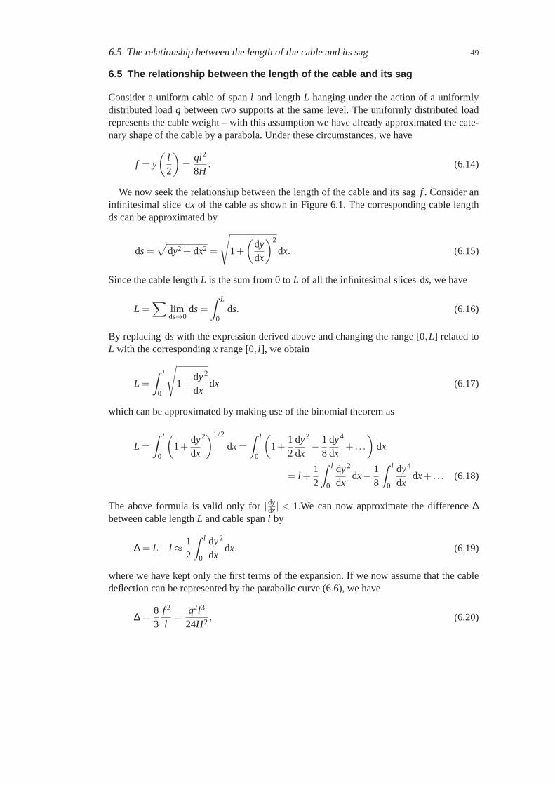
6.5 The relationship between the length of the cable and its sa g
Consider a uniform cable of spanl and lengthL hanging under the action of a uniformlydistributed loadq between two supports at the same level. The uniformly distributed loadrepresents the cable weight – with this assumption we have already approximated the cate-nary shape of the cable by a parabola. Under these circumstances, we have
f = y
(l2
)
=ql2
8H. (6.14)
We now seek the relationship between the length of the cable and its sagf . Consider aninfinitesimal slice dx of the cable as shown in Figure 6.1. The corresponding cable lengthds can be approximated by
ds =√
dy2+ dx2 =
√
1+
(dydx
)2
dx. (6.15)
Since the cable lengthL is the sum from 0 toL of all the infinitesimal slices ds, we have
L =∑
limds→0
ds =∫ L
0ds. (6.16)
By replacing ds with the expression derived above and changing the range [0,L] related toL with the correspondingx range [0, l], we obtain
L =
∫ l
0
√
1+dydx
2
dx (6.17)
which can be approximated by making use of the binomial theorem as
L =
∫ l
0
(
1+dydx
2)1/2
dx =∫ l
0
(
1+12
dydx
2
− 18
dydx
4
+ . . .
)
dx
= l +12
∫ l
0
dydx
2
dx− 18
∫ l
0
dydx
4
dx+ . . . (6.18)
The above formula is valid only for|dydx | < 1.We can now approximate the difference∆
between cable lengthL and cable spanl by
∆ = L− l ≈ 12
∫ l
0
dydx
2
dx, (6.19)
where we have kept only the first terms of the expansion. If we now assume that the cabledeflection can be represented by the parabolic curve (6.6), we have
∆ =83
f 2
l=
q2l3
24H2 , (6.20)

50 Chapter 6 Transverse deflection of cables
y
x
q1q2
l/2l/2
Figure 6.6
from which we can express the cable length asL = l +∆.The approximation (6.19) is valid in most of the cases of practical interest. The correction
to ∆ is indeed very small for a sag-to-span ratiof/l = 0.1:
∆ =83
f 2
l
(
1− 125
f 2
l2 + . . .
)
=83
110
f (1−0.024+ . . .) . (6.21)
6.5.1 On the principle of superposition for a cable under non -uniform load
The peculiarity of cables stems from their extreme flexibility resulting in big structuralchanges which are very much influenced by how the load is applied. Consider for instancethe system in Figure 6.6. The differential equation (6.4) cannot be used due to the discon-tinuity at the midspan. We can however solve the differential equation in eachof the twodomains and “join” the two contributions by means of some compatibility conditions atthemidspan. The problem is completely specified by considering two boundary conditions atthe two ends (deflection equal to zero) plus a displacement compatibility and anequilib-rium condition at the midspan – the latter matching condition implies that the tension, i.e.the vertical forces in the cable, must be the same. By using these four conditions we derivethe expression of the deflection in the two parts and, by (6.19) and∆ = L− l, givenL andl,the horizontal force
H2 =l3
384∆(5q2
1+6q1q2+5q22
). (6.22)
Evidently, the principle of superposition cannot be applied.Let us now take a different look at the non-uniform load in this example. Itis evident that
we can consider that non-uniform load as the sum of a uniform and a contra-symmetric loadas shown in Figure 6.7. By means ofp0 andq0 we redefine the applied load asq1 = q0+ p0

6.5 The relationship between the length of the cable and its sag 51
q1
q2
q0 = 12 (q1+q2)
p0 = 12 (q1−q2)+
−
+
+
=
+y
x
Figure 6.7
andq2 = q0− p0. Hence, the cable forceH in (6.22) can be expressed as
H2 = H20
(
1+14
(p0
q0
)2)
, (6.23)
where
H20 =
q20l3
24∆(6.24)
is the horizontal cable force when the contra-symmetric load is zero (p0 = 0).By an appropriate choice of the ratiop0/q0 we are allowed to say thatH is linearly
proportional, in an approximate way of course, to the applied load. Indeedby selectingp0 = 1/4q0 we have that
H2 = H20
(
1+164
)
= H20 (1+0.0156) , (6.25)
which means thatp0 increases the square of the horizontal component of the cable tensionby 1.56% (andH by 0.78%). Under these circumstances, the system acts close to linear andthe principle of superposition holds (in an approximate way).
6.5.2 The horizontal deflection of cables
Let us have a better look at what happens to the cable depicted in Figure 6.6. Since thereis more load on the left-hand side, the shape of the cable will be different from that of aparabola. The loading condition will also shift the middle point of the cable to theleft andevery point of the cable will suffer a horizontal and a vertical displacement u(x) andv(x).

52 Chapter 6 Transverse deflection of cables
A
By
dy
α
ds
dx
−du
x
y
v+ dvα
dv
u
v
A′
B′
αB′′
Figure 6.8
We can derive a relationship betweenu andv by considering a differential element of lengthds as shown in Figure 6.8.
To set the scene, consider the element ds in its initial configuration due to the uniformload q0 and in its deformed consideration after the application of the loadp0 (the load isnow q0+ p0). The deformed configuration can be identified by a vertical displacementv, ahorizontal displacementu and a rotationα aboutA′ to A′B′′ which takes place starting fromthe segment in the positionA′B′ – note thatA′B′ is inclined asAB.
Since we consider only small displacements,v << y and the arcB′B′′ can be replacedby a perpendicular line toA′B′. This implies that pointB, which is nowB′, undergoes anextra vertical displacement dv and an extra horizontal displacement−du. By eliminatingtanα from the expression of du obtained considering the triangle with the segmentB′′B′ ashypotenuse,−du = dv tanα , and from dy derived considering the initial configuration ofthe cable segmentAB, dy = dx tanα , we have
du =−dv tanα =−dvdydx
(6.26)
which can be rewritten as
dudx
=−dvdx
dydx
. (6.27)
The horizontal displacement can now be found by integration:
u =
∫
du =−∫
dvdx
dydx
dx+C1. (6.28)
Hence, given the deflections due to the uniform loadq0 (i.e. y) and to the contra-symmetricload p0 (i.e. v) it is possible to express the horizontal displacement of the cable. The inte-gration constant can be found with the conditionu(0) = 0.

6.5 The relationship between the length of the cable and its sag 53
(b)(a) M
l/2 l/4
Figure 6.9
p+q
f
l/2
f ∗
Figure 6.10
6.5.3 Cable stiffening
How do we stiffen a cable as to reduce its horizontal displacement? One simple way is toadd an inextensible tension wire like depicted in Figure 6.9.
Consider the case depicted in Figure 6.9(a) under the action of a uniform load q and acontra-symmetric loadp. Obviously, the deflection at midspan is due toq only (the contra-symmetric loadp does not produce any deflection at midspan due to symmetry). Further,due to the tension wire, the horizontal deflection is zero. Hence, as a goodapproximation ofthe original system we consider the cable depicted in Figure 6.10 and termf ∗ the deflectionat midspan. Worth noting is that the deflection line corresponding to the initial load q isnot influenced by the additional loadp (it is still a parabola!). However, the forceH haschanged and its value follows from
H +∆H =(p+q)
(l2
)2
8 f ∗=
(q+ p) l2
8 f(6.29)
where we considered the reduced system withH the original horizontal cable force,∆Hthe extra contribution coming from the stiffening cable, andf ∗ = 1/4 f where f is thedeflection at midspan of the whole system (f = ql2/8H). The expressionf ∗ = 1/4 f derivesfrom f = pl2/8H if we consider half cable spanl∗ = 1/2l; alternatively this expression canbe easily derived asf ∗ = v(l/4)− f/2 with v the deflection of the parabolic cable found

54 References
∆H
∆H
2∆H
carrier cable
tension wire
Figure 6.11
solving the differential equation of the cable with the boundary conditions ˜v(0) = 0 andv(l/2) = f .
After simple manipulations, the increase in cable force reads as
∆H =pl2
8 f. (6.30)
This force is provided by the tension wire at the pointM.Since the load in the right part of the cable is in the upward direction, the cableforce in
that point has decreased with an equal amount∆H. So, also this part of the cable causes atpoint M a force to the left on the tension wire. The sum of booth forces (2∆H) is carried bythe right hand part of the tension wire (see Figure 6.11).
Exercises
6.1
6.2
References
[1] H. M. Irvine. Cable Structures. Dover, Mineola, N.Y., 1992.
[2] H. M. Irvine and G. B. Sinclair. The suspended elastic cable under the action of concentrated vertical loads.International Journal of Solids and Structures, 12:309–317, 1976.
[3] S. Nedev. The catenary – an ancient problem on the computer screen. European Journal of Physics,21:451–457, 2000.
[4] Wikipedia. Catenary.http://en.wikipedia.org/wiki/Catenary , Accessed 7 August, 2009.
[5] Wikipedia. Capilano suspension bridge. http://en.wikipedia.org/wiki/Capilano_Suspension_Bridge , Accessed 2 July, 2008.

Chapter 7
Combined systems
Combined systems are structural systems in which different components contribute tothe global load-carrying capacity. In these systems, the applied load is redistributed tothe various components as a function of the corresponding stiffness. Suspension bridgesare amongst the most common combined systems.
7.1 Spring systems as prototypes of combined systems
Springs are flexible elastic devices used to store and release energy. Springs can be com-bined in series, parallel and in parallel/series assemblages. Any spring orspring system canbe characterized by its spring constantk which can be determined by Hooke’s lawF = ku,whereF is the applied force andu the resulting displacement (see Figure 7.1).
7.1.1 Hooke’s law
Hooke’s law of elasticity states that the extension of an elastic spring is linearlyproportionalto the applied force through a constant of proportionally called the spring constant. Thislaw is valid up to the elastic limit after which springs enter the plastic regime and sufferirrecoverable plastic deformation.
The law is named after the 17th century physicist Robert Hooke who described it byusing stretched springs as shown in Figure 7.2. This law holds also for compression springsunder physical constraints to prevent buckling. In 1676, Robert Hooke announced the law
to be of Robert Hookea portrait claimed by historian Lisa Jardine
Robert Hooke
⋆ Freshwater, Isle of Wight, England, July 18, 1635
† London, England, March 3, 1703
English polymath who played an important role in the scientific revolu-
tion, through both experimental and theoretical work.
In 1660, he discovered Hooke’s law of elasticity, which describes the
linear variation of tension with extension in an elastic spring.
Hooke coined the biological termcell.
55

56 Chapter 7 Combined systems
x = 0
compressed
equilibrium
stretchedFs < 0
Fs > 0
Fs = −kx
x > 0
x < 0
Figure 7.1 Hooke’s law: the negative sign inFs shows that any movement on the springwill be resisted by an equal but oppositeforce. The spring force is a restoring forceand acts in the opposite direction from the di-rection in which the system is displaced. Theorigin has to be placed at the position wherethe spring system would be in equilibrium forthe equationFs =−kx to be valid (in this po-sition the net force on the object to which thespring is attached is equal to zero. If not, thenFs = −k (x− x0) wherex0 is equilibrium po-sition relative to the origin.
that bears his name by using the anagramceiiinosssttuv. In 1678 he explained it asut tensiosic vis, Latin for the stretch is proportional to the force, which is comprehensible only tothe initiates. Fortunately, in his “Lectures on Natural Philosophy” (1807),Thomas Youngdemystified Hooke’s law by expressing it as the equationF = ku. Young, however, failed inreproducing the terseness of Hooke’s original enunciate [1]:
. . . the modulus of elasticity of any substance is a column of the same substance,capable of producing a pressure on its base which is to the weight causingacertain degree of compression as the length of the substance is to the diminutionof its length . . .
7.1.2 Springs in parallel and in series
Parallel and series systems of springs are the two ways to arrange a set of springs. Thesesystems are shown in Figures 7.3 and 7.6.
The equivalent spring constant for the parallel system in Figure 7.3 is derived by express-ing the translational equilibrium in the horizontal direction for the free body diagram shownin Figure 7.3(b). This results in the equation
F = F1+F2 = k1u1+ k2u2 = (k1+ k2)u, (7.1)
where we have used Hooke’s law to express the relation between force and displacementin the springs. We have also assumed that both springs undergo the same deformationu(= u1 = u2)), so that only one degree of freedom suffices to describe the system. Fromthe above equation we define the equivalent spring constant aske = k1+ k2. This result canbe generalizes for a system ofN springs in parallel:
ke =N∑
i=1
ki. (7.2)
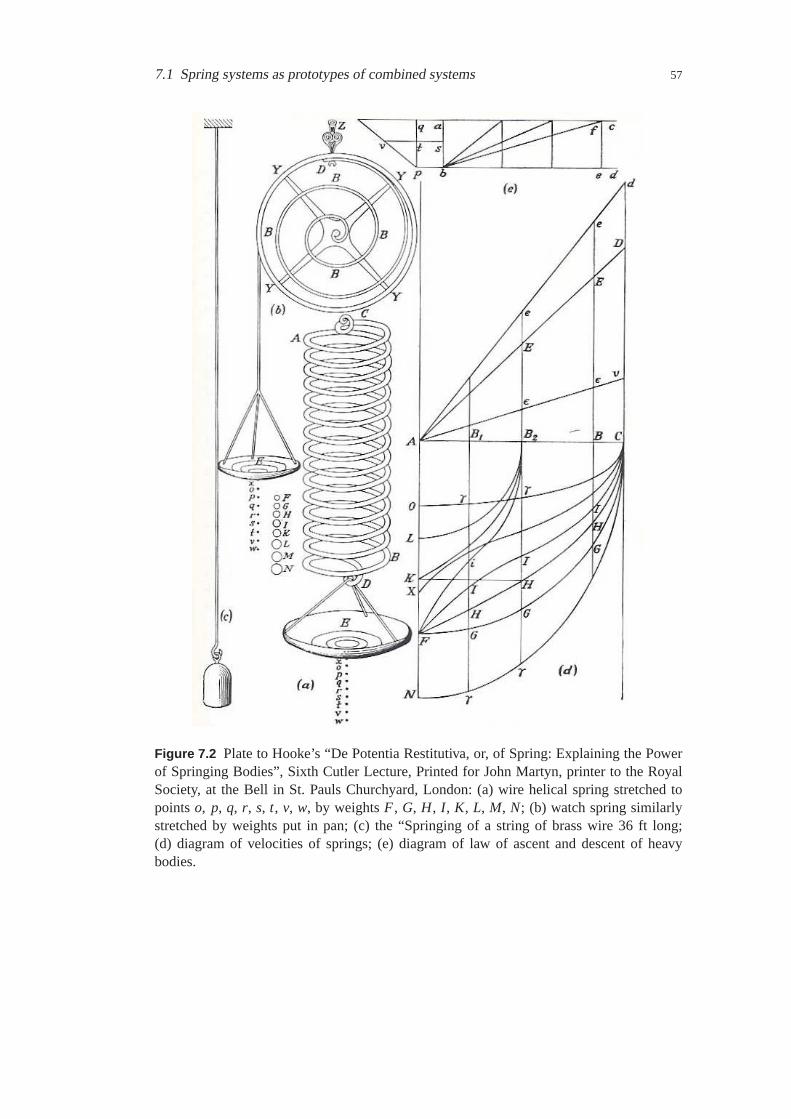
7.1 Spring systems as prototypes of combined systems 57
Figure 7.2 Plate to Hooke’s “De Potentia Restitutiva, or, of Spring: Explaining the Powerof Springing Bodies”, Sixth Cutler Lecture, Printed for John Martyn, printer to the RoyalSociety, at the Bell in St. Pauls Churchyard, London: (a) wire helical spring stretched topointso, p, q, r, s, t, v, w, by weightsF , G, H, I, K, L, M, N; (b) watch spring similarlystretched by weights put in pan; (c) the “Springing of a string of brass wire 36 ft long;(d) diagram of velocities of springs; (e) diagram of law of ascent and descent of heavybodies.

58 Chapter 7 Combined systems
(b)x
k2
k2
k1
(a) (c)
F2
F1F
k1
F
x
F
Figure 7.3 Springs in parallel.
k1l
a
b
(a) (b)
α
u2
u1
u
k2
F
Figure 7.4 A parallel combination of springs (unsymmetric case).
In the above derivations we have assumed that the springs are constrained as to undergothe same deformation. This was achieved by preventing the vertical bar to undergo anyrotation.
By releasing the rotation constraint, the system shown in Figure 7.4 has two degreesof freedom, a translation and a rotation. The extensional equivalent spring constant in thedirection of the horizontal applied forceF can be found by expressing the horizontal dis-placementu of the point of application of the load as a function of the two spring stiffnesses.This is easily accomplished by noting thatu1−u = a tanα andu−u2 = b tanα (these equa-tions have been obtained by considering similar triangles in Figure 7.4). By eliminatingtanα we obtain
u = u1bl+u2
al. (7.3)
The forceFi in each spring can be expressed as a function of the applied forceF by imposingthe rotational equilibrium at the two points where the springs are attached to thevertical bar.FromF1l = Fb andF2l = Fa, and by using Hooke’s law for the two springs, we obtain
u = F
(b2
k1l2 +a2
k2l2
)
=Fke, (7.4)

7.1 Spring systems as prototypes of combined systems 59
k2k1
∞8
21
0.5
a/l
k e/k
1
21.510.50-0.5-1
100
10
1
0.1
Figure 7.5 Equivalent spring constant for an unconstrained parallel combination of springsfor various ratiosk2/k1.
from which the equivalent spring constant for unconstrained parallelsprings can be ex-pressed as
ke =l2k1k2
a2k1+b2k2. (7.5)
This results is valid also when the forceF is not applied between the two springs.Following Folkerts [2], some insight into (7.5) can be gained by consideringits adimen-
sional form,
ke
k1=
k2/k1
(a/l)2+(1−a/l)2 k2/k1, (7.6)
for various ratiosk2/k1. Figure 7.5 shows that the equivalent spring constant for a systemof two unconstrained parallel springs depends on the location of the applied force.
We now consider some limiting cases of (7.5).(a) a = 0 or b = 0: The force is applied in line with one spring andke = k1 or ke = k2,respectively.(b) a → ∞ or b → ∞: ke → 0 which implies that the system becomes less stiff as the leverarm becomes longer.(c) k1 → ∞ or k2 → ∞: One of the two springs behaves like a rigid constraint andke →l2k2/a2 or ke → l2k1/b2, respectively. This implies that as the distance between the appliedforce and the rigid constraint increases the spring constant rapidly drops.Quoting Folkerts [2]:

60 Chapter 7 Combined systems
Fk2
x
xk1
k1
p
k2(a) (b)
Figure 7.6 Springs in series.
When two springs are not constrained to compress the same amount, a situationcommon in physics problems and in real life, then the textbook result ofke =k1+ k2 is often a poor approximation to the correct value.
Suppose now that we are interested in finding where to apply the loadF such that the bardoes not rotate after the application of the load. The condition to enforce is that u1 = u2 or,equivalently,F1/k1 = F2/k2. By using the expression previously derived forF1 andF2, theconstraint on the displacement yields the relationak1 = bk2.
When springs are in series, like in the system depicted in Figure 7.6, the force in eachspring equals the applied force:F = F1 = F2. The total deformation, on the other hand, isthe sum of the deformations of the single components and is given by
u = u1+u2 =F1
k1+
F2
k2= F
(1k1
+1k2
)
. (7.7)
Hence the equivalent spring constant is
ke =Fu=
11k1+ 1
k2
. (7.8)
In general, for a system ofN springs in series, we have that
1ke
=N∑
i=1
1k1. (7.9)
By using the previous concepts is possible to derive the equivalent stiffness of combinedsystem, like the one shown in Figure 7.7. The equivalent stiffness of this system is equal to
ke =1
1k1+k2+k1
+ 1k3+k3
. (7.10)

7.2 Beam-cable systems: Deflection of stiffened suspension bridges 61
k1
k2
k1
k3
k3
F
Figure 7.7 A parallel-series combination of springs.
7.2 Beam-cable systems: Deflection of stiffened suspension bridges
A stiffened suspension bridge is defined as a bridge with a stiff horizontaldeck “where thedeck load is carried vertically (or mostly vertically) by suspenders up to cables that transferthe loads by nearly horizontal forces to towers and then over them to side spans ending inheavy concrete anchorages” [3]. This system is also called a two-hinged truss suspensionbridge [4].
In these structural systems, the transverse deflection is reduced by the introduction of astiffening beam. A schematic is depicted in Figure 7.9 and consists of a single span cablestiffened by a simply supported beam of constant cross section. With reference to Figure 7.8,this could be considered as a good approximation of the part of the bridge between the twotowers.
7.2.1 Key assumptions
The assumptions in the analysis of two-hinged truss suspension bridges are as follow [4],[5, Section 11.3]:
• the dead load of the structure, uniformly distributed along the span, is entirely trans-mitted to the cable which takes a parabolic form;
• the initial dead load is carried by the cable with no bending in the beam;
• the stiffening beam has constant moment of inertiaEI (this is not essential, just asimplification);
• there is a continuous sheer of vertical hangers connecting the cable to the stiffeninggirder;
• the hangers are vertical in all deflected configurations of the structurei.e. the inclina-tion of the hangers may be neglected under live loads;
• axial elastic deformation of towers and hangers are neglected.

62 Chapter 7 Combined systems
7.2.2 Governing equation and its solution
The photo of the Clifton suspension bridge in Figure 7.8 highlights one of the main con-stituents of a suspension bridge, the suspenders. Ironically, suspenders, or hangers, are notrepresented in schematics of suspension bridges. Their “contribution” ishowever key to thederivation of the differential equation.
Consider the schematic of a suspension bridge shown in Figure 7.9. Here we have con-sidered a suspension bridge as a system composed by a bending beam withflexural stiffnessEI and a cable with no bending stiffness (EI = 0) and negligible extension (EA = ∞) con-nected by means of rigid hanger cables, not shown in the figure, with no extension under theaction of a distributed load. The space between hangers is considered to be small comparedto the bridge span so that the hangers can be considered as continuouslydistributed alongthe span. A live load produces deflection of both cable and bending beam.
The inextensibility of the hanger cables is the most important characteristic of the systemas it allows us to relate the deflectionvb of the beam and thatvc of the cable through theequation
vb (x) = vb (x)(= v(x)) . (7.11)
One of the implications of this assumption is that load redistribution can be easily definedby assigning a portionqc of the total loadq to the cable and the remainder of the load(qb = q−qc) to the beam. By assuming the same transverse displacementv we have defineda parallel system and separated the two components: we have a cable under the action of
Figure 7.8 Clifton suspension bridge, Bristol, England. The Clifton Suspension Bridgewas designed as the longest single-span road bridge in the world (span:214 m). It spansthe Avon Gorge and links Clifton in Bristol to Leigh Woods in North Somerset. Thebridge was designed by Isambard Kingdom Brunel; its construction begunin 1831 andwas completed in 1864 (photo courtesy of Erik Stensland, Morning Light Photography,http://morninglight.us).

7.2 Beam-cable systems: Deflection of stiffened suspension bridges 63
vc
q
cable
y, v
x
vb
Figure 7.9
x
Hq
EI, L
y
Figure 7.10
loadqc and a beam under the action of loadqb = q−qc. Both components are described bythe same transverse deflectionv. We can therefore write the governing equations for cableand beam separately as
cable: Hd2vdx2 =−qc, beam: EI
d4vdx4 = qb = q−qc. (7.12)
A single differential equation in terms of the transverse deflectionv can be finally obtainedby eliminating the cable loadqc:
EId4vdx4 −H
d2vdx2 = q. (7.13)
Equation (7.13) describes the behavior of the combined, parallel cable-beam system. Thesame equation can be derived by considering the vertical equilibrium for both cable andbeam of a differential element dx.
As a side remark, it is worth noticing that the transverse deflection of a simply sup-ported beam under the combined action of an axial tensile load and a distributed load isalso governed by (7.13). Further, a prestressed concrete girder can be regarded as a par-allel cable-beam system. The beam shown in Figure 7.10 can be related to thesuspensionbridge by noticing that the differential equation (7.13) remains valid for beam-cable systemswith hangers of zero length – indeed, we did not consider the length of the hangers in thederivation of (7.13).
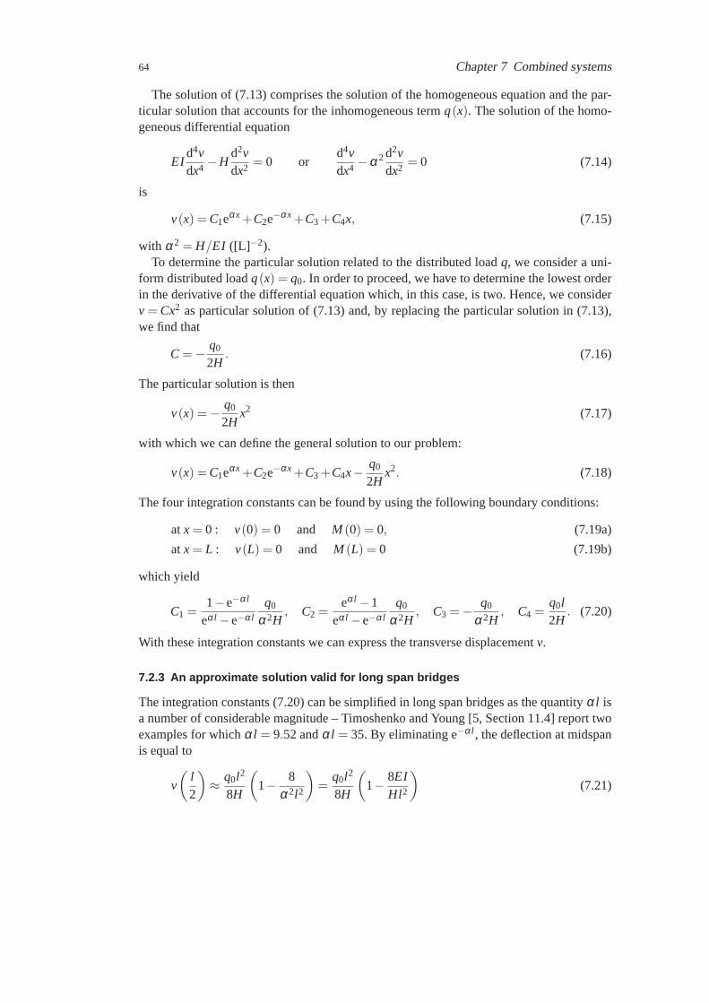
64 Chapter 7 Combined systems
The solution of (7.13) comprises the solution of the homogeneous equation and the par-ticular solution that accounts for the inhomogeneous termq(x). The solution of the homo-geneous differential equation
EId4vdx4 −H
d2vdx2 = 0 or
d4vdx4 −α2d2v
dx2 = 0 (7.14)
is
v(x) =C1eαx +C2e−αx +C3+C4x, (7.15)
with α2 = H/EI ([L] −2).To determine the particular solution related to the distributed loadq, we consider a uni-
form distributed loadq(x) = q0. In order to proceed, we have to determine the lowest orderin the derivative of the differential equation which, in this case, is two. Hence, we considerv = Cx2 as particular solution of (7.13) and, by replacing the particular solution in (7.13),we find that
C =− q0
2H. (7.16)
The particular solution is then
v(x) =− q0
2Hx2 (7.17)
with which we can define the general solution to our problem:
v(x) =C1eαx +C2e−αx +C3+C4x− q0
2Hx2. (7.18)
The four integration constants can be found by using the following boundary conditions:
at x = 0 : v(0) = 0 and M (0) = 0, (7.19a)
at x = L : v(L) = 0 and M (L) = 0 (7.19b)
which yield
C1 =1−e−αl
eαl −e−αl
q0
α2H, C2 =
eαl −1eαl −e−αl
q0
α2H, C3 =− q0
α2H, C4 =
q0l2H
. (7.20)
With these integration constants we can express the transverse displacement v.
7.2.3 An approximate solution valid for long span bridges
The integration constants (7.20) can be simplified in long span bridges as the quantityα l isa number of considerable magnitude – Timoshenko and Young [5, Section 11.4] report twoexamples for whichα l = 9.52 andα l = 35. By eliminating e−αl, the deflection at midspanis equal to
v
(l2
)
≈ q0l2
8H
(
1− 8α2l2
)
=q0l2
8H
(
1− 8EIHl2
)
(7.21)

7.2 Beam-cable systems: Deflection of stiffened suspension bridges 65
γ
Rf
32.521.510.50
1
0.8
0.6
0.4
0.2
0
Figure 7.11
which can be compared to the cable sag
f =q0l2
8H(7.22)
of an unstiffened suspension bridge. It is thus evident that in a stiffened suspension bridgethe ratioEI/Hl2 is responsible for the reduction of the stresses in the beam. A direct con-sequence of this finding is the possibility of using beams with smaller cross sections.
7.2.4 Sinusoidal load function
The effect of the axial load can be better appreciated if we assume a load function of thetype
q(x) = q0sinπxl. (7.23)
The solution of the governing equation is then given by
v(x) =1
1+ HEI
(lπ)2
q0
EI
(lπ
)4
sinπxl, (7.24)
while the bending moment
M (x) =−EId2vdx2 =
1
1+ HEI
(lπ)2 q0
(lπ
)2
sinπxl. (7.25)

66 Chapter 7 Combined systems
Both expressions contains the reduction factor
R f =1
1+ HEI
(lπ)2 . (7.26)
It is worth noticing that by lettingH = 0 we recover the solution of a bending beam withoutaxial force.
The reduction factor can be made a function of the Eulerian buckling load ofa beamPE = π2 EI
l2 :
R f =1
1+ HEI
(lπ)2 =
1
1+ HPE
=1
1+ γ(7.27)
with the parameterγ equal to the ratio of the cable force to the Eulerian buckling force.The influence of the reduction factor onv(x) andM (x) can be appreciated by analyzing thecurve shown in Figure 7.11.
Example 7.1 (Seabed pipe-laying)The problem of seabed pipe-laying can be analyzed by using (7.14). Consider the figurebelow where a vessel is positioning a cable on the bottom of the sea. In placing the cable,the vessel exerts a horizontal tensionH in the cable.
The problem consists in defining the point at which the cable is in perfect contact withthe sea floor given the forceH, the weight of the cableq, the stiffnessEI and the depth ofthe waterh.
h
x
y, v
l
H
We take as origin of the coordinate system the boat and consider that the cable is subjectedto its own weightq which we imagine as the applied loadq acting on the suspension bridge.The general solution of (7.14) is
v =C1eαx +C2e−αx +C3+C4x− q2H
x2, (7.28)

7.2 Beam-cable systems: Deflection of stiffened suspension bridges 67
where the last term comes into play because we have a distributed load. This equation can besolved considering four boundary conditions. The first two are specified atx = 0: v = 0 andM = 0. The remaining boundary conditions are defined by determining the point at whichthe cable is in perfect contact with the sea floor. We place this point atx = l. Hence, atx = lwe havedv
dx = 0 as the slope of the cable is zero – the cable is horizontal – andM = 0. Withthese boundary conditions we find
C1 =q
α2He−αl, C2 =
qα2H
, C3 =− qαH
, C4 =qlH
− qαH
, (7.29)
which yield the expression of the deflection
v =q
α2H
(
e−α(l−x)+e−αx −1)
+
(qlH
− qαH
)
x− 12
qH
x2. (7.30)
At x = l we find
v(l) =− qlαH
+12
qH
l2 (7.31)
from which, usingv(l) = h we can find the lengthl.
Example 7.2 (Parabolic roof structures)
roof plate
rib
cable
xH H
f
y, v
The deflection of roof structures can be reduced by adding flexural ribs. Let us take a lookat a simple model of a roof structure like the parabolic roof structure depicted in the figureabove. In the construction of such a structure, the first step is to hung cables between the twovertical beams. Next, roof plates are added on the cables and then concrete ribs are casted.The total weightq of the cables, plating and ribs is carried by the cables and the governing

68 Chapter 7 Combined systems
equation for this system is
−Hd2ydx2 = q. (7.32)
Since the load is distributed along the curve, the shape should be a catenary, but we canapproximate it by a parabola, Therefore, we may say that the force in the roof structure is
H =qL2
8 f. (7.33)
Well, now the roof is pretty solid, concrete has hardened and we are ready to have a partyon it. In doing so, we load the roof with some extra loadp which causes an extra deflectionv. Part of the load will be carried by the cable and part by the concrete ribs. Note that theconcrete ribs have used the cable to define their shape. Of course, extra deflection meansextra force∆H in the structure which is nowH +∆H. We indicate byqb the force takenby the ribs and therefore the load taken by the cable isqc = q+ p− qb whereq+ p is theapplied load. The implicit assumption is that since cable and ribs are glued together theywill undergo the same deformation. We have a parallel system. Therefore we can draw thecontributions of the two systems as shown in the figure below.
H +∆H
qb
qb
yv
x
cable
rib
yv
q+ px
The governing equations are now
−(H +∆H)d2(y+ v)
dx2 = q+ p−qb, for the cable (7.34)
and
EId4vdx4 = qb for the ribs. (7.35)
Here we have usedv since the ribs have been created on the shape given byy. Eliminatingqb we have
EId4vdx4 −H
d2ydx2 −∆H
d2ydx2 − (H +∆H)
d2vdx2 = q+ p. (7.36)

7.3 Shear beam-bending beam systems 69
Since−H d2ydx2 = q we have
EId4vdx4 − (H +∆H)
d2vdx2 =−∆H
Hq+ p. (7.37)
If ∆H is very small compared toH we may write
EId4vdx4 −H
d2vdx2 = p, (7.38)
which is the same equation we have seen for the suspension bridge.The ratio∆H/H is << 1 if we have a contra-symmetric load with small ratiop/q as we
have seen in Chapter 6.
7.3 Shear beam-bending beam systems
A common class of buildings is characterized by the presence of some walls made of con-tinuous slabs of concrete. The behavior of this kind of system is in betweenthat of a shearbeam and a bending beam. Generally speaking, when a building is much widerthan it istall we can consider the bending to be approximately zero and we call this system a shearbeam – this is due to the fact that the total stiffness against shear is given by the shear mod-ulus times the cross sectional area; hence, a wide building is dominated by shear and notby bending. On the other hand, when the the height of the building is large compared tothe width, the building deforms primarily by bending. Note however that if we assume thatthe building has a square cross section of widthw, the building becomes very stiff againstflexure asw becomes large.
7.3.1 Basic assumptions
Shear beams are an important component in many buildings. They are usuallyrigidly con-nected to beams with flexural stiffness like shown in Figure 7.12 and form a parallel system.
shear frame
front view
top view
bending beam
Figure 7.12

70 Chapter 7 Combined systems
lateral view top view
shear wall
rigid floor slabframes
shear wall
Figure 7.13
If this system is loaded with a horizontal system of forces, the frame and thebeam will ex-perience the same horizontal deflection.
Often, special shear walls are employed to sustain horizontal forces as shown in Fig-ure 7.13. In this case, the building is made of a number of slender high framesplaced nextto each other and is enclosured by flexible walls. A horizontal load is partly carried by theframes and partly transmitted to the shear walls via the floor slabs. If these floor slabs arerigid in their plane, the frames and walls experience equal displacements. This is also acombined system.
To investigate the behavior of this kind of combined system, we consider the structureshow in Figure 7.14a where a shear beam is connected with rigid members to a bendingbeam, or shear wall. Both beams are clamped to the foundation. In this case, the shear beamis subjected to a horizontal distributed loadq. As illustrated in Figure 7.14b the deformationof the two system, taken separately, is obviously different. However, when connected, theyare constrained to deform in a common deflected shape.
7.3.2 Governing equations and solution
Since the links are rigid, the displacements of frame and shear wall can be considered thesame:vs = vb. As a consequence, the bending beam carries a portionqb of the total loadq and the shear beam will carry the remaining partqs = q− qb. Similar to the case of thesuspension bridge, we have two separate structural systems, a shear wall under the actionof qb and a frame under the action ofqs = q− qb. The two systems are linked through the

7.3 Shear beam-bending beam systems 71
x
y, v
rigid linksq qb
(a) (b)
shear wallq
shear frame
l
k EI
Figure 7.14
displacementv. We can therefore write the following system of governing equations:
frame: − kd2vdx2 = qs = q−qb
beam: EId4vdx4 = qb
(7.39)
in which the only unknown isqb. Elimination ofqb yields
EId4vdx4 − k
d2vdx2 = q. (7.40)
This differential equation is similar to the one governing the deflection of the suspensionbridge (cf (7.13)). The boundary conditions are however differentand, with reference toFigure 7.14a, they are:
at x = 0 : v = 0 anddvdx
= 0;
at x = l : M =−EId2vdx2 = 0 and V =Vs +Vb = k
dvdx
−EId3vdx3 = 0.
Using these boundary conditions we find the expression of the transverse deflection and thebending moment:
v =ql2
GA
(
−1+α l sinhα l
(α l)2coshα l+
coshαx+α l sinhα (l − x)
(α l)2coshα l+
xl− x2
2l2
)
, (7.41)
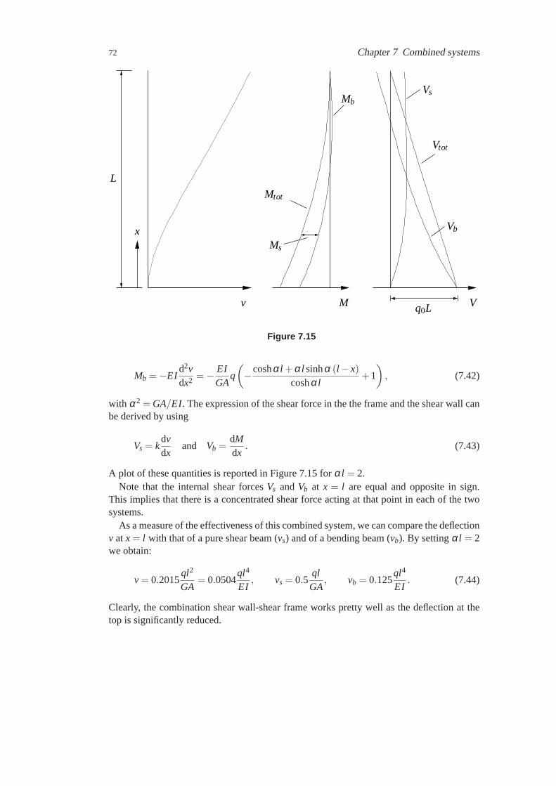
72 Chapter 7 Combined systems
v
x
L
Ms
M
Mb
Mtot
q0L V
Vtot
Vb
Vs
Figure 7.15
Mb =−EId2vdx2 =− EI
GAq
(
−coshα l +α l sinhα (l − x)coshα l
+1
)
, (7.42)
with α2 = GA/EI. The expression of the shear force in the the frame and the shear wall canbe derived by using
Vs = kdvdx
and Vb =dMdx
. (7.43)
A plot of these quantities is reported in Figure 7.15 forα l = 2.Note that the internal shear forcesVs andVb at x = l are equal and opposite in sign.
This implies that there is a concentrated shear force acting at that point in each of the twosystems.
As a measure of the effectiveness of this combined system, we can comparethe deflectionv at x = l with that of a pure shear beam (vs) and of a bending beam (vb). By settingα l = 2we obtain:
v = 0.2015ql2
GA= 0.0504
ql4
EI, vs = 0.5
qlGA
, vb = 0.125ql4
EI. (7.44)
Clearly, the combination shear wall-shear frame works pretty well as the deflection at thetop is significantly reduced.

References 73
Example 7.3 (Solving the shear wall-shear frame system with Maple)The differential equation (7.40) can be solved with the aid of a general-purpose computeralgebra system. An example of a Maple solution is reported below (courtesy of Hans Welle-man).M andV are the total moment and shear force of the system from equilibrium.> restart;
> alpha:=sqrt(k/EI);
> w:=C1+C2* x+C3* exp(-alpha * x)+C4 * exp(alpha * x)-(qo * xˆ2)/(2 * k);
w := C1+C2x+C3e(−
√
kEI x)
+C4e(√
kEI x)− qox2
2k> phi:=-diff(w,x): Va:=k * diff(w,x): kappa:=diff(phi,x):
> Mb:=EI * kappa:Vb:=diff(Mb,x):
> x:=0: eq1:=w=0: eq2:=phi=0:
> x:=L: eq3:=Mb=0: eq4:=Va+Vb=0:> sol:=solve( {eq1,eq2,eq3,eq4 }, {C1,C2,C3,C4 }): assign(sol);> x:=’x’:
> M:=(-1/2) * qo* (x-L)ˆ2: V:=diff(M,x):
> L:=10; EI:=10000; k:=400; evalf(alpha * L);qo:=5;> plot(w,x=0..L,y=0..(1/(8 * EI)) * qo* Lˆ4,title="displacement v",labels=["x[m]","v [m]"]);> plot([Va,Vb,V],x=0..L,y=(-1/2) * qo* L..qo * L,title="Shearforce",labels=["x [m]","V [kN]"],legend=["Va","Vb","V total"]);> plot([Mb,M],x=0..L,y=(-1/2) * qo* Lˆ2..(1/2) * qo* Lˆ2,title="Bendingmoment",legend=["Mb","M total"],labels=["x [m]","M [kN m]"]);
Exercises
7.1
7.2
References
[1] A. King. Plain text.MRS Bulletin, 31:72, 2006.
[2] T. J. Folkerts. A more general form for parallel springs.American Journal of Physics, 70(5):493–494,2002.
[3] Princeton University Art Museum. The art of structural design. http://www.princetonartmuseum.org/Bridges/glossary.html , Accessed 19 December, 2006.
[4] D. A. Morelli. Some Contributions to the Theory of Stiffned Suspension Bridge. PhD the-sis, California Institute of Technology, 1946.http://etd.caltech.edu/etd/available/etd-05142003-112733/unrestricted/Morelli_da_1946.pd f , Accessed 7 August, 2009.
[5] S. P. Timoshenko and D. H. Young.Theory of Structures. McGraw-Hill Book Company, New York, secondedition, 1965.

Chapter 8
Fundamentals of matrix structural analysis:The matrix displacement method
The matrix displacement method is a numerical procedure to determine displacementand stress fields of a structural system under the action of applied loads.The matrixdisplacement method can be considered as a form of the finite element method.There is a plethora of documentation on all aspects of matrix structural analysis. Anexcellent starting point is the historical outline by Felippa [1] and references therein.For those interested in a complete reference, the book by Przemieniecki [2] is a must.This chapter is based on [2, 3].
8.1 Introduction
Given a physical system, in the matrix displacement method we seek a relation, set in amatrix form of the type
ka = f , (8.1)
between applied forcesf and unknown displacementsa through a stiffness matrixk. Hencethe definition “matrix displacement method”. In structural systems, the arraya containsnodal unknowns such as axial extensions, transverse deflections and rotations while thearray f collects the corresponding axial forces, shearing forces and bending moments.k isthe stiffness of the complete system, also known as global stiffness matrix, and is given by
k =Nel
Ae=1
ke, (8.2)
whereke is the element stiffness matrix.A indicates the assembly operator which scatters thedegrees of freedom from the element to the structure. The assembly operator can be replacedby the summation operatorΣ provided that the element stiffnesses are fully expanded to theglobal matrix.
A typical analysis involves the following steps:
1. idealization of the physical system;
2. discretization of the mathematical model;
3. application of the matrix displacement method procedure;
75

76 Chapter 8 Fundamentals of matrix structural analysis: The matrix displacementmethod
Figure 8.1 Stringer and Wall model of a beam (from Model Code 90)
4. solution of the equations;
5. evaluation of stresses;
6. interpretation of numerical results.
The idealization of the physical system (step 1), a structure in our case, consists in its re-duction to simpler units, like if the structure were a Lego assembly – an example is reportedin Figure 8.1. For each of these units, or finite elements, we seek the stiffness propertiesin terms of force-displacement relations (step 2). Through assembly (step3), we define theforce stiffness relation of the global structure which, once solved (step4), yields the soughtdisplacements. Given the displacement field, we can derive the strain and stress fields (step5). The final step, usually the most difficult, consists in understanding the outcome of thenumerical analysis (step 6).
8.2 The force-displacement relationship
There are many ways to derive the force-displacement relationship of individual elements:the unit-displacement theorem, Castigliano’s theorem, the solution of the differential equa-tions for the element displacements, variational methods. These methods are detailed inCook et al. [3], Buchanan [4], Przemieniecki [2] and Hughes [5]. Here we shall use the so-lution of the differential equation. The stiffness matrices derived with this method, as wellwith that of the methods above are exact within the limit of validity of the differential equa-tion in the sense that no further approximations will be used to derive the stiffness matrix.This method is however limited to simple elements and is restricted to situations in whichactual displacements are assumed to be small (i.e. we can approximate cosθ by 1 and sinθby 0) and the material of the structural member obeys linear elasticity.
The result of this operation can be condensed into
ka = f or ki, ja j = fi, (8.3)
whereki, j is the reaction (axial force, bending moment, shearing force) at the degree of free-domi due to a unit deformation (translation, rotation, deflection) at the degree offreedomj.In other words, a column ofk lists nodal loads that must be applied to nodal degrees of free-dom in order to create the deformation state associated with unit value of the correspondingelement degrees of freedom while all other element degrees of freedomare zero.

8.3 Axial deformation 77
N1
N1
x
u2, N2u1, N1
+
N
(a)
(b)N2
u2 = 0
N2
u1 = 0x
u2
u1
(c)
(d)
Figure 8.2
Next, we determine the stiffness matrices of uniform and weightless bar and beam ele-ments taking into account the definition of the stiffness coefficientski, j just given.
8.3 Axial deformation
We consider a bar finite element with one axial degree of freedom per node. Positive ax-ial displacements and forces are depicted in Figure 8.2(b) while Figure 8.2(a) reports theconvention for positive axial internal forces. The differential equation governing the axialdisplacementu in the uniform bar shown in Figure 8.2(c) is
N (x) = EAdudx
. (8.4)
This differential equation is integrated directly to obtain
u(x) =N (x)EA
x+C1, (8.5)
whereC1 is an integration constant. Making use of the boundary condition atx = 0 (u =u1) we deriveC1 = u1. The second boundary condition atx = l (u = u2 = 0) yieldsN2 =−u1EA/L. From the equilibrium equationN1 =−N2 we obtainN1 = u1EA/L. Hence
k1,1 =N1
u1=
EAL
(8.6)
and
k4,1 =N2
u1=−EA
L. (8.7)
The remaining terms of the stiffness matrix can be derived by symmetry or by consideringthe bar shown in Figure 8.2(d). Following the above procedure we obtaink4,4 = k1,1 andk1,4 = k4,1.
Note that we have used the ordering in (8.35) for the coefficientski, j.

78 Chapter 8 Fundamentals of matrix structural analysis: The matrix displacementmethod
Quantity Definition
curvature κ = d2vdx2
bending moment M = EIκshear force V = dM
dx
distributed load q = dVdx
Table 8.1 Summary of governing equation for beam with sign convention of Figure 8.3.
8.4 Shear and bending deformation
The beam element has four degrees of freedom: a displacement perpendicular to the axis ofthe beam and a rotation at each end. Nodal forces corresponds to nodal displacements whilenodal moments corresponds to nodal rotations. Sign conventions are shown in Figure 8.3while the corresponding governing equation are summarized in Table 8.1. Note that nodalmomentsMi are positive in the direction of nodal rotationsθi.
When bending and shearing strains are present, the transverse deflection of the beam isgiven by the sum of the bending and shearing contributions
v = vb + vs. (8.8)
The bending deflection is governed by the differential equation
EId2vb
dx2 =V1x−M1, (8.9)
where the right-hand side is defined as the moment acting at distancex from left-hand endof the beam. The shear deflectionvs is such that
dvs
dx=− V1
GAs, (8.10)
whereAs represents the beam cross sectional area effective in shear. By integrating (8.9)twice, replacingvb = v−vs in this equation and consideringvs from the integration of (8.10)
+V :
+M:
+q:
x
y +
κv1, V1 v2, V2
θ1, M1 θ2, M2
+
z
Figure 8.3 Conventions for a beam element: (a) positive curvatureκ, (b) forces on an in-finitesimal beam element, (c) degrees of freedomv1, v2 andθ1, θ2 with associated nodalforcesV1, V2 and momentsM1, M2.

8.4 Shear and bending deformation 79
V1
M1 V2
M2
θ1 = 0
v1
θ2 = 0v2 = 0
v2
V1
M1
V2
M2
θ2 = 0θ1 = 0v1 = 0
(a) (b)
Figure 8.4 Deformation states associated with the activation ofv1 andv2.
we obtain
EIv =16
V1x3− 12
M1x2+
(
C1−EIV1
GAs
)
x+C2 (8.11)
with C1 andC2 integration constants.
8.4.1 Shear
The boundary conditions related to Figure 8.4(a) for (8.11) yield [6, Section 7.12]
dvdx
=dvs
dx=− V1
GAsat x = 0, x = L (8.12)
and
v = 0 at x = L, (8.13)
from which
C1 = 0 (8.14)
and
C2 =112
LV1
GAs
(12EI +GAsL
2) , (8.15)
where we have considered thatM = 0 atx = L/2 andM1 = V1L/2. With these integrationconstants, (8.11) becomes
EIv =V1x3
6− M1x2
2− V1ΦL2
12x+
112
L3V1(1+Φ) (8.16)
where
Φ =12EI
GAsL2 (8.17)

80 Chapter 8 Fundamentals of matrix structural analysis: The matrix displacementmethod
θ2 = 0v2 = 0
V2
M2θ1
v1 = 0
V1
M1
θ1 = 0v1 = 0
θ2
v2 = 0
M2V1 V2
M1
(b)(a)
Figure 8.5 Deformation state associated with the activation ofθ1 andθ2.
is a dimensionless coefficient.By using equilibrium we can define the remaining forces acting on the beam asV2 =−V1
andM2 =−M1+V1L.We are now ready to define the coefficients of the stiffness matrix. According to the
definition ofki, j and with the ordering in (8.35), lettingv = v1 at x = 0, we have
v1 = (1+Φ)L3V1
12EI(8.18)
from which
k2,2 =V1
v1=
12EI(1+Φ)L3 , (8.19)
k3,2 =M1
v1=
V1L2v1
=6EI
(1+Φ)L2 , (8.20)
k5,2 =V2
v1=− 12EI
(1+Φ)L3 , (8.21)
and
k6,2 =−M1+V1L
v1=
6EI(1+Φ)L2 . (8.22)
The remaining coefficients in the second column are zero.If the left-hand end of the beam is built-in as in Figure 8.4(b) we can, by symmetry
considerations or by using the differential equation, derive the remainingcoefficients:
k5,5 = k2,5 =12EI
(1+Φ)L3 , k6,5 = k3,5 =−k6,2 =− 6EI(1+Φ)L2 . (8.23)
8.4.2 Bending
In order to define the stiffness coefficients associated with the rotationsθ1 andθ2 we subjectthe beam to bending moments and the associated shear forces as shown in Figure 8.5. Equa-tion (8.11) is still valid but the boundary conditions need to be adapted to the new loading

8.4 Shear and bending deformation 81
condition. With reference to Figure 8.5(a) we have
v = 0 at x = 0, x = L (8.24)
and
dvdx
=dvs
dx=− V1
GAsat x = L. (8.25)
With v = 0 atx = 0 we obtainC2 = 0, whilev = 0 atx = L yields
V1L3
6− M1L2
2+
(
C1−EIGA
V1
)
L = 0. (8.26)
The boundary condition (8.25) givesC1 = M1L− V1L2
2 . By replacingC1 in (8.26) we obtainthe following relation betweenV1 andM1:
V1 =6M1
(4+Φ)L. (8.27)
The equations derived before are still valid and we report them below:
V2 =−V1, M2 =−M1+V1L. (8.28)
We are now ready to derive the coefficientski, j. At x = 0 we have
dvb
dx=
dvdx
− dvs
dx= θ1 (8.29)
which implies
θ1 =M1(1+Φ)LEI (4+Φ)
(8.30)
from which
k3,3 =M1
θ1=
(4+Φ)EI(1+Φ)L
, (8.31)
k5,3 =V2
θ1=− 6EI
(1+Φ)L2 (=−k2,3 =−V1
θ1), (8.32)
and
k6,3 =M2
θ1=
−M1+V1Lθ1
=(2−Φ)EI(1+Φ)L
. (8.33)
If the deflection of the left-hand end of the beam is zero as shown in Figure8.5(b) it isthen evident from symmetry that
k6,6 = k3,3 =(4+Φ)EI(1+Φ)L
. (8.34)
The remaining coefficients can be derived in a similar manner.

82 Chapter 8 Fundamentals of matrix structural analysis: The matrix displacementmethod
8.5 Putting it all together: the plane frame element
Assembling the terms corresponding to axial, shear and flexural deformation, we arrive atthe stiffness matrix of a two dimensional frame element:
N1
V1
M1
N2
V2
M2
=
EAL 0 0 −EA
L 0 0
0 12EIL3(1+Φ)
6EIL2(1+Φ)
0 − 12EIL3(1+Φ)
6EIL2(1+Φ)
0 6EIL2(1+Φ)
(4+Φ)EIL(1+Φ) 0 − 6EI
L2(1+Φ)(2−Φ)EIL(1+Φ)
−EAL 0 0 EA
L 0 0
0 − 12EIL3(1+Φ)
− 6EIL2(1+Φ)
0 12EIL3(1+Φ)
− 6EIL2(1+Φ)
0 6EIL2(1+Φ)
(2−Φ)EIL(1+Φ) 0 − 6EI
L2(1+Φ)(4+Φ)EIL(1+Φ)
u1
v1
θ1
u2
v2
θ2
. (8.35)
8.6 Reduction to particular cases
8.6.1 Truss element
The truss element is the simplest structural elements. It has only one degreeof freedomassociated with each node and is obtained by considering only the degreesof freedom cor-responding to axial deformation in (8.35):
[N1
N2
]
=EAL
[1 −1
−1 1
][u1
u2
]
. (8.36)
8.6.2 Beam element
There are two major beam theory, the Timoshenko beam and the Euler-Bernoulli beam.Both assume no axial deformation.
Timoshenko beam
The Timoshenko beam accounts for transverse shear deformation and isobtained by ne-glecting axial deformation in (8.35):
V1
M1
V2
M2
=
12EIL3(1+Φ)
6EIL2(1+Φ)
− 12EIL3(1+Φ)
6EIL2(1+Φ)
6EIL2(1+Φ)
(4+Φ)EIL(1+Φ) − 6EI
L2(1+Φ)(2−Φ)EIL(1+Φ)
− 12EIL3(1+Φ)
− 6EIL2(1+Φ)
12EIL3(1+Φ)
− 6EIL2(1+Φ)
6EIL2(1+Φ)
(2−Φ)EIL(1+Φ) − 6EI
L2(1+Φ)(4+Φ)EIL(1+Φ)
v1
θ1
v2
θ2
. (8.37)

8.7 The assembly procedure 83
Euler-Bernoulli beam
The Euler-Bernoulli is the classical formulation for beams and is obtained byneglecting theeffects of shear deformation in (8.37). This is accomplished by setting the shear deformationparameterΦ to zero:
V1
M1
V2
M2
=
12EIL3
6EIL2 −12EI
L36EIL2
6EIL2
4EIL −6EI
L22EI
L
−12EIL3 −6EI
L212EI
L3 −6EIL2
6EIL2
2EIL −6EI
L24EI
L
v1
θ1
v2
θ2
. (8.38)
8.6.3 Properties of the element stiffness matrix
• The stiffness matrices of the frame element (8.35), the truss element (8.36), the Tim-oshenko beam element (8.37), and the Euler-Bernoulli beam element (8.38) are allsingular and symmetric.
• Singularity of the stiffness matrix is caused by the linear relations introducedby theequilibrium equations. In the bar element, the first row is equal to the secondrow butfor the minus sign. In the beam element we encounter a similar situation for rows1and 3 plus the relationL times row 1 minus row 2 equals row 4. Physically, it meansthat the element can undergo rigid body motion due to insufficient constraints.
• The stiffness matrix is symmetric and this can be justified with the reciprocal theoremof Maxwell-Betti.
• When displacement are directly proportional to the applied loads the stiffness matrixis always symmetric.
• A stiffness termski, j is zero unless at least one element is attached to both degree offreedomi and j.
• Diagonal terms are non-negative. If a diagonal term is zero, then deformation with nostrain energy is possible (this is the case of a mechanism).
8.7 The assembly procedure
As briefly discussed in the introduction, in the matrix displacement method we seek a rela-tion of the type
ka = f (8.39)
valid at the structural level in which
k =Nel
Ae=1
ke, (8.40)
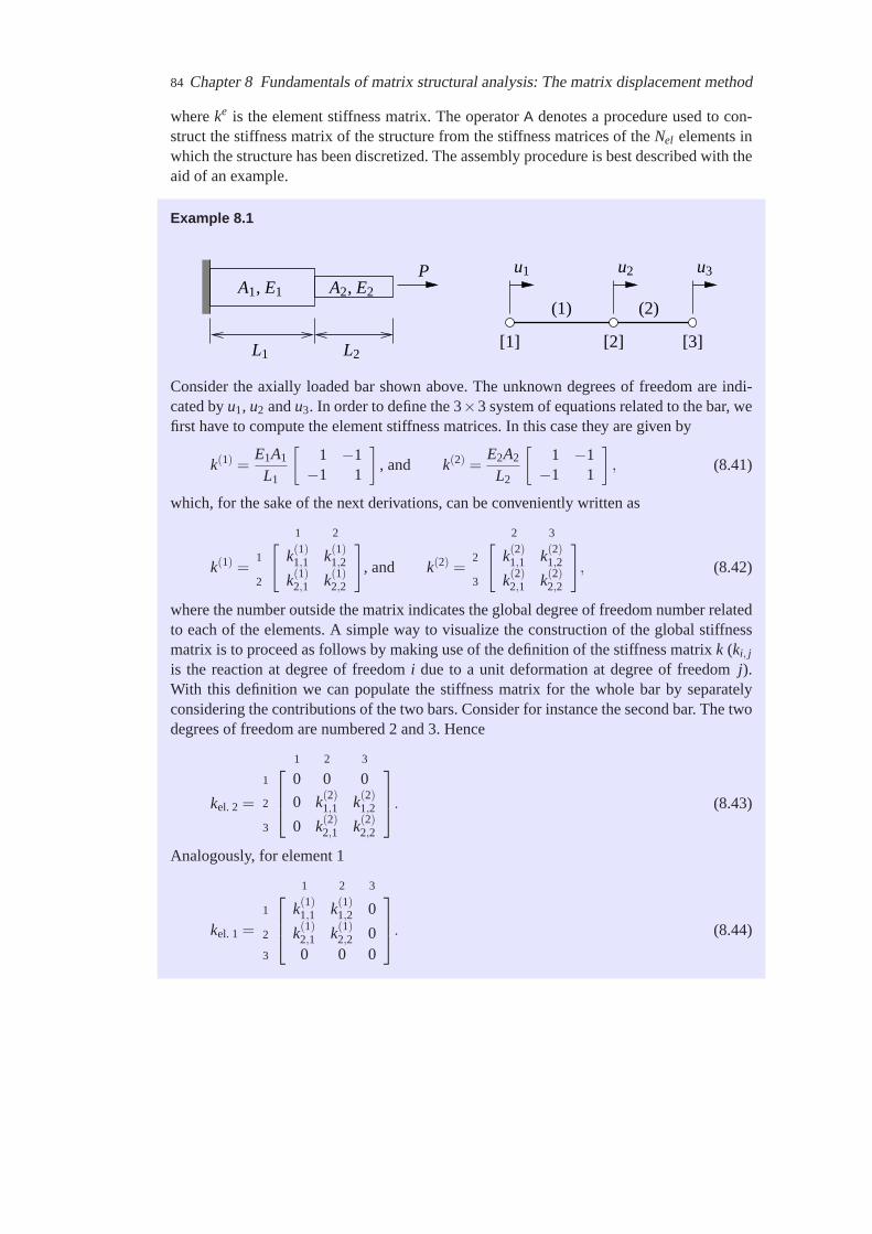
84 Chapter 8 Fundamentals of matrix structural analysis: The matrix displacementmethod
whereke is the element stiffness matrix. The operatorA denotes a procedure used to con-struct the stiffness matrix of the structure from the stiffness matrices of theNel elements inwhich the structure has been discretized. The assembly procedure is best described with theaid of an example.
Example 8.1
u1 u3u2
[3][2][1]
(1) (2)
L1 L2
A1, E1 A2, E2
P
Consider the axially loaded bar shown above. The unknown degrees offreedom are indi-cated byu1, u2 andu3. In order to define the 3×3 system of equations related to the bar, wefirst have to compute the element stiffness matrices. In this case they are given by
k(1) =E1A1
L1
[1 −1
−1 1
]
, and k(2) =E2A2
L2
[1 −1
−1 1
]
, (8.41)
which, for the sake of the next derivations, can be conveniently written as
k(1) =
[1 2
1 k(1)1,1 k(1)1,2
2 k(1)2,1 k(1)2,2
]
, and k(2) =
[2 3
2 k(2)1,1 k(2)1,2
3 k(2)2,1 k(2)2,2
]
, (8.42)
where the number outside the matrix indicates the global degree of freedom number relatedto each of the elements. A simple way to visualize the construction of the global stiffnessmatrix is to proceed as follows by making use of the definition of the stiffness matrix k (ki, j
is the reaction at degree of freedomi due to a unit deformation at degree of freedomj).With this definition we can populate the stiffness matrix for the whole bar by separatelyconsidering the contributions of the two bars. Consider for instance the second bar. The twodegrees of freedom are numbered 2 and 3. Hence
kel. 2=
1 2 3
1 0 0 0
2 0 k(2)1,1 k(2)1,2
3 0 k(2)2,1 k(2)2,2
. (8.43)
Analogously, for element 1
kel. 1=
1 2 3
1 k(1)1,1 k(1)1,2 0
2 k(1)2,1 k(1)2,2 03 0 0 0
. (8.44)

8.7 The assembly procedure 85
Adding the two contributions, we arrive at the stiffness matrix for the whole bar:
k =
1 2 3
1 k(1)1,1 k(1)1,2 0
2 k(1)2,1 k(1)2,2+ k(2)1,1 k(2)1,2
3 0 k(2)2,1 k(2)2,2
. (8.45)
The applied load must be assembled as well. It is applied in correspondenceof the thirddegree of freedom. Hence
f =
1 R2 03 P
. (8.46)
Note the reaction forceR in the RHS. This is an additional unknown in this problem.What is left to do is to solve the systemka = f for the displacement vectora =
[u1, u2, u3]. Note that the matrixk is singular (its inverse does not exist!). This meansthat the bar is not constrained and can undergo rigid body motion–with reference to thedifferential equation related to this problem, it is like if we were trying to solve it withoutconsidering boundary conditions. To constrain the bar we have to specify the value of asufficient number of degrees of freedom. In this simple one-dimensional example the ap-plication of the displacement boundary condition related to the node 1 suffices. Practically,this is done by striking out the row and the column related to that degree of freedom. Thisoperation yields the 2×2 system
[2 3
2 k(1)2,2+ k(2)1,1 k(2)1,2
3 k(2)2,1 k(2)2,2
][u2
u3
]
=
[2 03 P
]
(8.47)
which can be easily solved. The row-striking technique just described can be applied withhomogeneous constraints (u1 = 0). The recipe for the general case of non-homogeneousconstraints like e.g.u3 = u is discussed in Section 8.10.
8.7.1 The matrix assembly procedure in a finite element code
A widely used procedure consists in defining a connectivity arrayld for each element (ldis acronym for ”local degrees of freedom”). In this array local degrees of freedom are linkedto global degrees of freedom. In this exampleld (1) = [1,2] and ld (2) = [2,3], where thearray indexi defines the local element degree of freedom andld (i) the global degree offreedom number. These arrays can be used to populate the global stiffness matrix by usingAlgorithm 1. An example is reported in the code listed on page 91.

86 Chapter 8 Fundamentals of matrix structural analysis: The matrix displacementmethod
Input : ld , number of elements, number of element degrees of freedom (do f ),element stiffness matrixk(e)
Output: global stiffness matrixk
zero global stiffness matrixk1
for each element e do2
for i = 1, dof do3
for j = 1, dof do4
kld (i),ld ( j) = kld (i),ld ( j)+ k(e)i, j5
end6
end7
end8
Algorithm 1: Assembly procedure.
β = α
αx
y′
y
x′
o, o′
Figure 8.6
8.8 Transformations
We have computed element arrays such as stiffness matrices and force vectors in local co-ordinates with the aim of ease computations of these quantities. However, beams and barsare arbitrarily placed and this requires a way to express element arrays ina generic sys-tem knowing their expression in the local coordinate systems. This can be accomplished bymaking use of some simple manipulations.
8.8.1 Transformation of vectors
This section is based upon [3, Section 7.2]. Consider a vectorV which can be thought of asa force vector, a displacement vector etc. The components ofV in the reference systemxoyare(Vx, Vy). The same vector can be defined in a systemx′o′y′ rotated of an angleα withrespect to the reference system. We call the systemx′o′y′ the local coordinate system. Thecomponents ofV in the local system are
(Vx′ , Vy′
).

8.8 Transformations 87
Our goal is to express(Vx′ , Vy′
)in terms of(Vx, Vy) and of the cosines of the angles
between the two systems. These cosines are called direction cosines.The direction cosines of thex′ axis are indicated by(lx′ , mx′) and those of they′ axis by
(ly′ , my′
). We know, from analytical geometry that we can expressVx′ as the sum of the
projection ofVx andVy along thex′ axis asVx′ = lx′Vx +mx′Vy. The componentVy′ can beexpressed in a similar way. In matrix format these two expressions reads
(Vx′
Vy′
)
=
[lx′ mx′
ly′ my′
](Vx
Vy
)
= R
(Vx
Vy
)
. (8.48)
The matrixR is orthogonal (R−1 = RT) and corresponds to pure rotation since detR = 1.With reference to Figure 8.6 we have thatlx′ = cosα , mx′ = cos(π/2−α) = sinα ,
ly′ = cos(π/2+β ) = cos(π/2+α) = −sinα , andmy′ = cosβ = cosα . We can thereforeexpress the rotation matrix as
R =
[cosα sinα
−sinα cosα
]
. (8.49)
8.8.2 Transformation of element arrays
The stiffness matrix of the bar element has been expressed as a function of the two degreesof freedomu1 andu2 in the local system (see (8.36)). It is however convenient, in view of itsexpression in the globalxoy coordinates system, to express it as a function of four degreesof freedom, two in the axial direction,u′1 andu′2, and two normal to the bar axis,v′1 andv′2. A similar transformation can be done on the local force array. Hence, starting from thestiffness matrix
[u′1 u′2
u′1 k1,1 k1,2
u′2 k2,1 k2,2
]
, (8.50)
the augmented stiffness matrix reads
u′1 v′1 u′2 v′2
u′1 k1,1 0 k1,2 0v′1 0 0 0 0u′2 k2,1 0 k2,2 0v′2 0 0 0 0
. (8.51)
Next, the arraya′ = [u′1, v′1, u′2, v′2]T is expressed as a function of the arraya =
[u1, v1, u2, v2]T in the global coordinate system through the use of the transformation ma-
trix
T4×4
=
[R 00 R
]
. (8.52)

88 Chapter 8 Fundamentals of matrix structural analysis: The matrix displacementmethod
Hence,a′ = T a, f ′ = T f , andk′a′ = f ′ can be written asT Tk′T a = f which yields thestiffness matrix of a bar element inclined of an angleα in thexoy coordinate system:
k = T Tk′T =EAL
[k0 −k0
−k0 k0
]
, (8.53)
where
k0 =
[c2 cscs s2
]
(8.54)
with c = cosα ands = sinα . From a practical point of view, it is convenient to retain thestructure of the stiffness matrix of the truss in the original 2×2 format and use a differenttransformation matrix. By using the 2×4 transformation matrix
T =
[lx′ mx′ 0 00 0 lx′ mx′
]
(8.55)
and the 2×2 element stiffness matrix (see (8.36)), we arrive at the same expressionof the4×4 stiffness matrix in thexoy coordinate system. For a frame element with the degrees offreedom ordered as in (8.35), the transformation matrix is [2, page 82]
T6×6
=
[R 00 R
]
(8.56)
with
R =
lx′ mx′ 0ly′ my′ 00 0 1
=
cosα sinα 0−sinα cosα 0
0 0 1
. (8.57)
The next example shows how to apply the transformation procedure described above.
Example 8.2This example is a slight modification of the one found in the book by Przemieniecki [2,Section 6.9]. Consider the statically undetermined pin-jointed truss shown in thenextfigure. The structure is loaded by a vertical force at node 1. The numbering for elements,nodes and degrees of freedom is shown in the figure together with the dimension of thetruss, the intensity of the load and the boundary conditions (nodes 3 and 4 are constrainedin both directions). Other data are listed in the next table where thep−q direction for eachmember is identified by the node numbers, and the direction cosines are defined in thexoycoordinate system by means of the node coordinates. The Young’s modulus of the materialis 10×106 N/mm2.

8.8 Transformations 89
o
(2)
(4)
5
6
1
2
3
4
7
8
20 cm
20 cm
P2 = 1000 Ny
x
(1)
(5)
[1]
[2][4]
[3]
(6) (3)
Member number Cross-sectional area Length Location Direction cosinesi Ai [mm2] Li [mm] p−q lpq mpq
1 1.0 20 3,1 1 02
√2/2 20
√2 4,1
√2/2
√2/2
3 1.0 20 1,2 0 -1.04
√2/2 20
√2 3,2
√2/2 -
√2/2
5 1.0 20 4,2 1.0 06 1.0 20 3,4 0 -1.0
The stiffness matrix for a pin-jointed truss in thexoy coordinate system is defined throughk = T Tk′T wherek′ is the stiffness matrix (8.36) defined in a local coordinate system andTis the transformation matrix (8.55). Hence
k(1) =
5 6 1 2
5 1 0 −1 06 0 0 0 01 −1 0 1 02 0 0 0 0
0.5×10⁶ Nmm
, (8.58)

90 Chapter 8 Fundamentals of matrix structural analysis: The matrix displacementmethod
k(2) =
7 8 1 2
7 1 1 −1 −18 1 1 −1 −11 −1 −1 1 12 −1 −1 1 1
0.125×10⁶ Nmm
, (8.59)
k(3) =
1 2 3 4
1 0 0 0 02 0 1 0 −13 0 0 0 04 0 −1 0 1
0.5×10⁶ Nmm
, (8.60)
k(4) =
5 6 3 4
5 1 −1 −1 16 −1 1 1 −13 −1 1 1 −14 1 −1 −1 1
0.125×10⁶ Nmm
. (8.61)
Noting thatk(5) = k(1) and k(6) = k(3), the element matrices are then assembled into theglobal system stiffness matrix of the structure. This leads to
k =
1 2 3 4 5 6 7 8
1 52 1 5 symmetric3 0 0 54 0 −4 −1 55 −4 0 −1 1 56 0 0 1 −1 −1 57 −1 −1 −4 0 0 0 58 −1 −1 0 0 0 −4 1 5
0.125×10⁶ Nmm
. (8.62)
Similarly, assembly of the global force array yields
f =
1 02 10003 04 05 06 07 08 0
N. (8.63)
Removing row and columns of constrained degrees of freedom (5 to 8) wemay now writethe equilibrium equations as
ka = f (8.64)

8.9 A minimal Matlab/Octave 2D finite element truss code 91
or
1 2 3 4
1 5 1 0 02 1 5 0 −43 0 0 5 −14 0 −4 −1 5
0.125×10⁶ Nmm
a1
a2
a3
a4
=
1 02 103
3 04 0
N (8.65)
from which
a = k−1 f =211
×10−3
−6305
25
mm. (8.66)
Once the displacements are known, we can derive the strain and stress fields in the truss.
8.9 A minimal Matlab/Octave 2D finite element truss code
The whole procedure described in Example 8.2 can be made automatic. A minimal Mat-lab/Octave 2D finite element code is listed below and can be downloaded from the courseweb page. The result of Example 8.2 is shown in Figure 8.7 with displacements magnified400 times.
% t r u s s .m%% a minimal Mat lab / Octave 2D f i n i t e e lemen t t r u s s code%% coded by Angelo Simone , TU De l f t , December 2007%
%% −− c l e a r memory%c l e a r a l l
%% −− g i ve t r u s s p r o p e r t i e s : noda l c o o r d i n a t e s ,% c o n n e c t i v i t y t a b l e , d e g r e s o f f reedom / node ,% a x i a l s t i f f n e s s%coord =[20 20 ; 20 0 ; 0 20 ; 0 0 ] ;conn =[3 1 ; 4 1 ; 1 2 ; 3 2 ; 4 2 ; 3 4 ] ;dofNode =2;E=10* 10ˆ6 ;A( 1 ) =1;A( 2 ) =s q r t ( 2 ) / 2 ;A( 3 ) =1;A( 4 ) =s q r t ( 2 ) / 2 ;A( 5 ) =1;A( 6 ) =1;

92 Chapter 8 Fundamentals of matrix structural analysis: The matrix displacementmethod
AE=A* E ;nNodes = s i z e(coord , 1 ) ;nElements = s i z e(conn , 1 ) ;
%% −− a l l o c a t e a r r a y s i n ka= f%nDofs =dofNode * nNodes ; % t o t a l number o f do f sk= z e r o s(nDofs , nDofs ) ; % s t i f f n e s s m a t r i xa= z e r o s(nDofs , 1 ) ; % s o l u t i o n a r r a yf = z e r o s(nDofs , 1 ) ; % r h s
%% −− d e f i n e boundary c o n d i t i o n s :% c o n s t r a i n e d do fs and a p p l i e d load%constrainedDofs =[5 6 7 8 ] ;f ( 2 ) =1000;
%% −− assemb le s t i f f n e s s m a t r i x%f o r e =1:nElements
% element c o n n e c t i v i t y t a b l eeleConn =conn (e , : ) ;
% e lemen t c o o r d i n a t e s and l e n g t hx1 =coord (eleConn ( 1 ) , 1 ) ;x2 =coord (eleConn ( 2 ) , 1 ) ;y1 =coord (eleConn ( 1 ) , 2 ) ;y2 =coord (eleConn ( 2 ) , 2 ) ;len = s q r t ( ( x2−x1 ) * (x2−x1 ) +(y2−y1 ) * (y2−y1 ) ) ;
% c and s a r e c o s i n e and s i n e o f t h e% an g le between l o c a l and g l o b a l axesc =(x2−x1 ) / len ;s =(y2−y1 ) / len ;
% e lemen t s t i f f n e s s m a t r i x ( l o c a l sys tem )ke_loc =AE(e ) / len * [1 0 −1 0 ;
0 0 0 0 ;−1 0 1 0 ;
0 0 0 0 ] ;
% r o t a t i o n and t r a n s f o r m a t i o n m a t r i xR=[c s ;
−s c ] ;
Zero =[0 0 ;0 0 ] ;
T=[R Zero ;Zero R ] ;
% e lemen t s t i f f n e s s m a t r i x ( g l o b a l sys tem )ke =T ' * ke_loc * T
% . . . f a s t e r a l t e r n a t i v e% ke=AE( e ) / l e n* [ c * c c* s −c* c −c* s ;% c* s s* s −c* s −s* s ;% −c* c −c* s c* c c* s ;

8.10 Constraints: application of prescribed displacements 93
% −c* s −s* s c* s s* s ]
% compute sys tem do fs a s s o c i a t e d wi th each e lemen t% ( node 1 has do fs 1 and 2 , node 2 has do fs 3 and 4 . . . )index ( 1 ) =dofNode * eleConn ( 1 ) −1;index ( 2 ) =dofNode * eleConn ( 1 ) ;index ( 3 ) =dofNode * eleConn ( 2 ) −1;index ( 4 ) =dofNode * eleConn ( 2 ) ;
% assemb le ke i n t o Kedof = l e n g t h( index ) ;f o r i =1:edof
ii =index ( i ) ;f o r j =1:edof
jj =index ( j ) ;k ( ii , jj ) =k ( ii , jj ) +ke ( i , j ) ;
endend
end
%% −− app ly boundary c o n d i t i o n s by z e r o i n g ou t% rows and colums and p u t t i n g ones on t h e d i a g o n a l%k (constrainedDofs , : ) =0;k ( : , constrainedDofs ) =0;k (constrainedDofs , constrainedDofs ) =eye( l e n g t h(constrainedDofs ) ) ;
%% −− s o l v e ka= f f o r a%a= inv (k ) * f
%% −− p l o t r e s u l t s%mag=400; % s c a l e f a c t o r f o r p l o tc l fho ld onf o r e =1:nElements
x=coord (conn (e , : ) , 1 ) ;y=coord (conn (e , : ) , 2 ) ;u=a (2* conn (e , : ) −1) ;v=a (2* conn (e , : ) ) ;t i t l e ( ' Deformed p l o t ')a x i s equalp l o t (x , y , ' r−−o ' )p l o t (x+mag* u , y+mag* v , ' k−o ' )
end
8.10 Constraints: application of prescribed displacements
Degrees of freedom can be given a value different than zero by following the proceduredescribed in this section. To this end, consider the relation
ka = f , (8.67)

94 Chapter 8 Fundamentals of matrix structural analysis: The matrix displacementmethod
0 5 10 15 200
5
10
15
20
Deformed plot
Figure 8.7 Truss after the application of the load (displacements are magnified 400 times).
and partition thea array in free and prescribed components:
a =
[a f
ap
]
. (8.68)
Consequently, the relation (8.67) can now be written as
[k f f k f p
kp f kpp
][a f
ap
]
=
[f f
f p
]
(8.69)
which can be re-written as
k f f a f + k f pap = f f (8.70a)
kp f ap + kppap = f p. (8.70b)
In the above system of equations, known quantities areap and f f (prescribed degrees offreedom and applied forces at free nodes) while unknown quantities area f and f p (unknowndegrees of freedom at free nodes and forces at constrained nodes, i.e. the reaction forces).
Considering equation (8.70a), it is possible to solve fora f :
k f f a f = f f − k f pap, (8.71)
where the effect of the prescribed degrees of freedom is expressed as extra forces appliedto the free degrees of freedom. Equation (8.70b) can be used to compute the reaction forcesonce the unknown vectora is known.
Splitting the relation (8.67) into two systems of equations and using only the first corre-sponds to cancelling the rows related to the prescribed degrees of freedom–this is indicatedas step 1 in the example below; moving the terms related toap to the RHS allows to solvefor a f –step 2 in the example below.

8.11 Equivalent concentrated forces 95
Example 8.3Let us reconsider Example 8.1 discussed in Section 8.7. We now constrain the third degreeof freedom to be equal to ¯u. With this constraint,
a =
u1
u2
u3
=
0u2
u
, (8.72)
while the RHS
f =
f1f2f3
=
R1
0R3
, (8.73)
whereRi are reaction forces. There are three unknowns in this problem:u2, R1, andR3 andthe stiffness matrix (8.45) is still valid.
To solve this problem we proceed as follows:
step 1 remove the equations related to known displacements (equations 1 and 3) in ka = f :
[1 2 3
2 k(1)2,1 k(1)2,2+ k(2)1,1 k(2)1,2
]
0u2
u
=[
0]
(8.74)
step 2 move the columns related to known displacements (columns 1 and 3) to the RHSmultiplying them by the corresponding displacement values (0 and ¯u):
[
k(1)2,2+ k(2)1,1
][u2]=[
0]−[
k(1)2,1
][0]−[
k(2)1,2
][u]
(8.75)
step 3 solve the system for the unknowns (u2 in this case):
u2 =−k(2)1,2
k(1)2,2+ k(2)1,1
u (8.76)
The last step usually implies the inversion of the matrixk f f .
8.11 Equivalent concentrated forces
To take into account distribute loads, we need to derive equivalent nodal forces. This isnecessary as we work with elements that accept only nodal contributions tothe RHS. Theenergy approach allows the computation of concentrated forces equivalent, in terms of work,to the corresponding distributed force.
We consider any one of the beam (or bar) dofsai to be of unit intensity and compute the
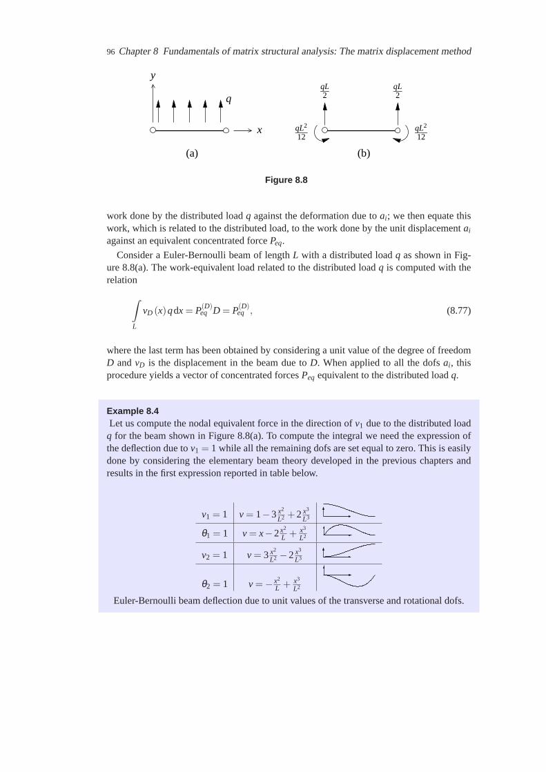
96 Chapter 8 Fundamentals of matrix structural analysis: The matrix displacementmethod
y
q
x
(a) (b)
qL2
qL2
qL2
12qL2
12
Figure 8.8
work done by the distributed loadq against the deformation due toai; we then equate thiswork, which is related to the distributed load, to the work done by the unit displacementai
against an equivalent concentrated forcePeq.
Consider a Euler-Bernoulli beam of lengthL with a distributed loadq as shown in Fig-ure 8.8(a). The work-equivalent load related to the distributed loadq is computed with therelation
∫
L
vD (x)qdx = P(D)eq D = P(D)
eq , (8.77)
where the last term has been obtained by considering a unit value of the degree of freedomD andvD is the displacement in the beam due toD. When applied to all the dofsai, thisprocedure yields a vector of concentrated forcesPeq equivalent to the distributed loadq.
Example 8.4Let us compute the nodal equivalent force in the direction ofv1 due to the distributed load
q for the beam shown in Figure 8.8(a). To compute the integral we need the expression ofthe deflection due tov1 = 1 while all the remaining dofs are set equal to zero. This is easilydone by considering the elementary beam theory developed in the previouschapters andresults in the first expression reported in table below.
v1 = 1 v = 1−3x2
L2 +2x3
L3
θ1 = 1 v = x−2x2
L + x3
L2
v2 = 1 v = 3x2
L2 −2x3
L3
θ2 = 1 v =− x2
L + x3
L2
Euler-Bernoulli beam deflection due to unit values of the transverse androtational dofs.
References 97
With this expression at hand, the nodal equivalent load is computed from
∫
L
vDqdx =∫
L
vv1qdx =∫
L
(
1−3x2
L2 +2x3
L3
)
qdx =12
qL = P(v1)eq . (8.78)
Considering all the remaining contributions we have
Peq = qL
1/2L/121/2
−L/12
. (8.79)
Peq is a vector of work-equivalent nodal loads. They are equivalent to support reactions fora uniform beam fixed at both ends and uniformly loaded with a load of intensity−q (seeFigure 8.8(b)). These nodal forces and moments are statically equivalent to the distributedforce: they have the same resultant force and moment about an arbitrarychosen point asdoes the original distributed loading.
The procedure described above can be used to compute nodal forcesequivalent to con-centrated forces applied between two nodes. In this case, the integral must be replaced bythe product of the deflection evaluated at the point of application of the force and the forceitself.
Exercises
8.1 Compute the stiffness matrix of a bar of embedded in a medium. The bar has lengthL and axial stiffnessEA. The action of the medium on the bar can be replaced by a set ofcontinuously distributed elastic forces of the typep = ku whereu is the axial displacementandk is the elastic stiffness of the medium. What happens to the stiffness matrix whenk → 0andk → ∞?
8.2 Demonstrate that the vector of work-equivalent nodal loads obtained employing a Tim-oshenko beam element is identical to that obtained with a Euler-Bernoulli beam when abeam is loaded by a uniformly distributed transverse load. What happens with an arbitrarilydistributed load?
References
[1] C. A. Felippa. A historical outline of matrix structural analysis: A play inthree acts.Computers andStructures, 79(14):1313–1324, 2001.
[2] J. S. Przemieniecki.Theory of Matrix Structural Analysis. Dover, Mineola, N.Y., 1985 (Originally pub-lished by McGraw Hill Book Company in 1968).
[3] R. D. Cook, D. S. Malkus, and M. E. Plesha.Concept and Applications of Finite Element Analysis. JohnWiley & Sons, New York, third edition, 1989.
[4] G. R. Buchanan.Finite Element Analysis. Schaum’s outline series. McGraw-Hill, New York, 1995.
98 References
[5] T. J. R. Hughes.The Finite Element Method - Linear Static and Dynamic Finite Element Analysis. Prentice-Hall, London, 1987.
[6] J. M. Gere and S. P. Timoshenko.Mechanics of Materials. Wadsworth, Inc., Belmont, California, secondedition, 1984.