An Introduction to Survey Methods and Techniques Methods and Techniques . An ... are not covered in this discussion but may be found in ... topographic points are measured by stadia

J. Paul Guyer, P.E., R.A. Editor

Paul Guyer is a registered civil engineer, mechanical engineer, fire protection engineer and architect with 35 years of experience designing buildings and related infrastructure. For an additional 9 years he was a principal staff advisor to the California Legislature on capital outlay and infrastructure issues. He is a graduate of Stanford University and has held numerous national, state and local offices with the American Society of Civil Engineers, Architectural Engineering Institute and National Society of Professional Engineers. He is a Fellow of ASCE and AEI.

An Introduction to Survey Methods and Techniques

An Introduction to

Survey Methods and Techniques

J. Paul Guyer, P.E., R.A.

Editor

The Clubhouse Press El Macero, California

CONTENTS 1. GENERAL

2. TOTAL STATIONS

3. REAL TIME KINEMATIC (RTK) GPS

4. TERRESTRIAL LIDAR (LASER) SCANNING

5. TOPOGRAPHIC DATA COLLECTION PROCEDURES

6. AUTOMATED FIELD DATA COLLECTION

7. METHODS OF DELINEATING AND DENSIFYING TOPOGRAPHIC FEATURES

(This publication is adapted from the Unified Facilities Criteria of the United States government which are in the public domain, have been authorized for unlimited distribution, and are not copyrighted.) (Figures, tables and formulas in this publication may at times be a little difficult to read, but they are the best available. DO NOT PURCHASE THIS PUBLICATION IF THIS LIMITATION IS UNACCEPTABLE TO YOU.)

© J. Paul Guyer 2015 1

1. OLDER TOPOGRAPHIC SURVEYING METHODS. This section provides an

overview of the past and present instruments and methods used to perform topographic

surveys of sites, facilities, or infrastructure. Prior to the advent of total stations, GPS,

LIDAR, and data collector systems, transit and plane table topographic surveying

methods and instruments were once standard. They are rarely used today, other than

perhaps for small surveys when a total station or RTK system is not available. However,

the basic field considerations regarding detail and accuracy have not changed, and field

observing methods with total stations or RTK are not significantly different from the

older survey techniques briefly described in the following sections.

1.1 TRANSIT-TAPE (CHAIN). Transit tape topographic surveys can be used to locate

points from which a map may be drawn. The method generally requires that all

observed data be recorded in a field book and the map plotted in the office. Angles from

a known station are measured from another known station or azimuth mark to the point

to be located and the distance taped (or chained) from the instrument to the point.

Transit-tape surveys typically set a baseline along which cross-section hubs were

occupied and topographic features were shot in on each cross-section. The elevation of

an offset point on a section is determined by vertical angle observations from the transit.

The slope or horizontal distance to the offset point is obtained by chaining. The

accuracy may be slightly better than the plane table-alidade method or very high (0.1 ft

or less), depending upon the equipment combinations used. Transits are still used by

some surveying and engineering firms, although on a declining basis if electronic total

station equipment is available. Transit-tape surveys can be used for small jobs, such as

staking out recreational fields, simple residential lot (mortgage) surveys, and aligning

and setting grade for small construction projects. Assuming the project is small and an

experienced operator is available, this type of survey method can be effective if no

alternative positioning method is available. Detailed procedures for performing and

recording transit tape topographic surveys can be found in most of the survey texts.


1.2 CHAINING. 100, 200, 300, or 500-foot steel tapes are used for manual distance

measurement methods. Woven, cloth, and other types of tapes may also be used for

lower accuracy measurements. Maintaining any level of accuracy (e.g., better than 1:

5,000) with a steel tape is a difficult process, and requires two experienced persons.

Mistakes/blunders are common. Tapes must be accurately aligned over the points

(using plumb bobs), held at a constant, measured tension, and held horizontally (using

hand levels). Subsequent corrections for tape sag/tension, temperature, and slope may

be necessary if a higher accuracy is required. Taping methods, errors, and corrections

are not covered in this discussion but may be found in any of the basic surveying texts.

1.3 TRANSIT-STADIA. Transit-stadia topographic surveys are performed similarly to

transit-tape surveys described above. The only difference is that distances to offset

topographic points are measured by stadia "tacheometry" means-- i.e., using the

distance proportionate ratio of the horizontal cross hairs in the transit telescope. The

multiple horizontal crosshairs in the transit scope can be used to determine distance

when observations are made on a level rod at the remote point. This distance

measurement technique has been used for decades, and is also the basis of plane table

survey distance measurement. The three horizontal crosshairs in the transit are spaced

such that the upper and lower crosshair will read 1.0 ft on a rod 100 ft distant from the

transit--a "stadia constant" ratio of 100:1. (Not all instruments have an even 100 : 1

stadia constant). The accuracy of a stadia-derived distance is not good—probably about

1 : 500 at best. Thus, a 500 ft shot could have an error of ± 1 ft. Additional errors (and

corrections) result from inclined stadia measurements, i.e., when the shot is not

horizontal. Reduction of the stadia intercept values to a nominal slope distance, then

reduction to horizontal, requires significant computation or use of tables. Transit-stadia

was often used like a modern day total station in that topo detail could be densified

(typically using radial survey methods) from a single instrument setup. All observed data

was recorded in a field book, and occasionally optionally plotted in the field. Transit-

stadia techniques are likewise rarely performed today if a total station is available.

Details on stadia measurement methods are found in any surveying textbook.


1.4 TRANSIT/THEODOLITE-EDM. Electronic Distance Measurement (EDM)

instruments were first developed in the 1950s, primarily for geodetic operations. In the

1970s, more compact EDM units were mounted atop or alongside transits and

theodolites--thus replacing manual chaining or optical stadia distance measurement.

Observed data were still recorded in field books for later office hand plotting. These

crude transit-EDM combinations were the early forerunner of the modern total stations.

During this time, methods were developed for automated drafting of observed features--

after individual angles and distances and features were encoded on punch cards and

input to a computer/plotter system.

Figure 2-5

Plane (no pun intended) table and alidade--Wild T-2 theodolite at right

(USC&GS, ca 1960s)


1.5 PLANE TABLE SURVEYING. The plane table and alidade were once the most

common tools used to produce detailed site plan maps in the field. The Egyptians are

said to have been the first to use a plane table to make large-scale accurate survey

maps to represent natural features and man-made structures. Plane table mapping is

rarely done today--plane table surveying has, for most purposes, been replaced by

aerial photogrammetry and total stations, but the final map is still similar. Plane table

surveys were performed well into the 1980s, and perhaps into the 1990s. A plane table

survey system is described as follows: A blank map upon which control points and grid

ticks have been plotted is mounted on the plane table. The table is mounted on a low

tripod with a specially made head--see Figure 2-5 above. The head swivels so that it

can be leveled, locked in the level position, and then be rotated so that the base map

can be oriented. The base map is a scaled plot of the ground control stations. Thus,

with the table set up over one of the stations, it can be rotated so that the plotted

stations lie in their true orientation relative to the points on the ground. Spot elevations

and located features are located with an alidade, an instrument that uses optical stadia

to determine distance (similar to the transit stadia). The error of a map produced with a

plane table and alidade varies across the map as the error in stadia measurements

varies with distance. Horizontal errors may range from 0.2 ft at 300 feet, to 10 ft or more

at 1,000 feet. Since the elevation of the point is determined from the stadia

measurement, relative errors in the vertical result. The plane table survey resulted in a

“field-finished” map product, with all quality control and quality assurance performed in

the field by the party chief/surveyor. The site plan map delivered from the plane table

was immediately suitable for overlaying design detail. Modern day electronic survey and

CADD systems are still attempting to attain the same level of “field-finish” capability that

the plane table once produced.


Figure 2-6

Leica TCR 705 Reflectorless Total Station


2. TOTAL STATIONS. Total stations were first developed in the 1980s by Hewlett-

Packard (Brinker and Minnick 1995). These instruments sensed horizontal and vertical

angles electronically instead of optically, and combined them with an EDM slope

distance to output the X-Y-Z coordinates of a point relative to the instrument's X-Y-Z

coordinates. Electronic theodolites operate in a manner similar to optical instruments.

Angle readings can be to 1" with precision to 0.5". Digital readouts eliminate the

uncertainty associated with reading and interpolating scale and micrometer data. The

electronic angle-measurement system eliminates the horizontal- and vertical-angle

errors that normally occur in conventional theodolites. Measurements are based on

reading an integrated signal over the surface of the electronic device that produces a

mean angular value and eliminates the inaccuracies from eccentricity and circle

graduation. These instruments also are equipped with a dual-axis compensator, which

automatically corrects both horizontal and vertical angles for any deviation in the plumb

line. An EDM device is added to the theodolite and allows for the simultaneous

measurements of the angle and the distance. With the addition of a data collector, the

total station interfaces directly with onboard microprocessors, external PCs, and

software. The ability to perform all measurements and to record the data with a single

device has revolutionized surveying. Total stations perform the following basic

functions:

Types of measurements:

Slope distance

Horizontal angle

Vertical angle

Operator input to total station data collector:

Text (date, job number, crew, etc.)

Atmospheric corrections (PPM)

Geodetic/grid definitions

HI & HR


Descriptor/attribute of setup point, backsight point, sideshot point, stakeout point,

etc.

In general, there are three types of total station operating modes:

Reflector--total station requires a solid reflector or retroreflector signal return from

the remote point to resolve digital angles and distances. Prisms are attached to a

pole positioned over a feature. Requires two-man field crew--operator and

rodman.

Reflectorless--the total station will resolve (and coordinate) signal returns off

natural features. Distances may be far more limited than those obtained from

reflectors ... typically less than 1,000 ft. Allows for more economical one-man

field crew operation.

Robotic--total station self-tracks single operator/rodman at remote shot or

stakeout points. One-man crew operation, with operator normally based at

remote rod point.


Figure 2-7

RTK base station and radio link transmitter--and rover with backpack


3. REAL TIME KINEMATIC (RTK) GPS. RTK survey methods have become widely

used for accurate engineering and construction surveys, including topographic site plan

mapping, construction stake out, construction equipment location, and hydrographic

surveying. RTK survey systems operate in a similar fashion as the robotic total station,

with one major exception being that a visual line of sight between the reference point

and remote data collection point is not required. Both RTK and total stations use similar

data collection routines and methods, and can perform identical COGO stake out

functions. Kinematic surveying is a GPS carrier phase surveying technique that allows

the user to rapidly and accurately measure baselines while moving from one point to the

next, stopping only briefly at the unknown points, or in dynamic motion such as a survey

boat or aircraft. A reference receiver is set up at a known station and a remote, or rover,

receiver traverses between the unknown points to be positioned. The data is collected

and processed (either in real-time or post-time) to obtain accurate positions to the

centimeter level. Real-time kinematic solutions of X-Y-Z locations using the carrier (not

code) phase are referred to as "real-time kinematic" (RTK) surveys. However, included

in this definition are "post-processed real-time kinematic" (PPRTK) techniques where

the kinematic solution is not actually performed in "real-time." RTK (or PPRTK) survey

techniques require some form of initialization to resolve the carrier phase ambiguities.

This is done in real-time using "On-the-Fly" (OTF) processing techniques. Periodic loss

of satellite lock can be tolerated and no static initialization is required to regain the

integers. This differs from other GPS techniques that require static initialization while the

user is stationary. A communication link between the reference and rover receivers is

required to maintain a real-time solution.


Figure 2-8

Optech LIDAR scanner and resultant image of underside of Bridge


4. TERRESTRIAL LIDAR (LASER) SCANNING. Laser scanning instruments have

been developed that will provide topographic detail of structures and facilities at an

extremely high density, as shown in Figure 2-8 above. These tripod-mounted

instruments operate similarly to a reflectorless total station. However, they are capable

of scanning the entire field of view with centimeter-level pixel density in some cases. A

full 3D model of a project site or facility results from the scan. This model must be edited

and feature attributes added.


5. TOPOGRAPHIC DATA COLLECTION PROCEDURES. Uniform operating

procedures are needed to avoid confusion when collecting topographic survey data,

especially for detailed utility surveys. The use of proper field procedures is essential to

prevent confusion in generating the final site plan map. Collection of survey points in a

meaningful pattern aids in identifying map features. The following guidelines are

applicable to all types of topographic survey methods, including total stations and RTK

systems.

5.1 ESTABLISH PRIMARY HORIZONTAL and vertical control for radial survey. This

includes bringing control into the site and establishing setup points for the radial survey.

Primary control is usually brought into the site from established NSRS

monuments/benchmarks using static or kinematic GPS survey methods and/or

differential leveling. Supplemental traverses between radial setup points can be

conducted with a total station as the radial survey is being performed. A RTK system

may require only one setup base; however, supplemental checkpoints may be required

for site calibration. Elevations are established for the radial traverse points and/or RTK

calibration points using conventional leveling techniques. Total station trigonometric

elevations or RTK elevations may be used if vertical accuracy is not critical--i.e., ± 0.1 ft.

5.2 PERFORM RADIAL SURVEYS to obtain information for mapping. Set the total

station or RTK base over control points established as described above. Measure and

record the distance from the control point up to the electronic center of the instrument

(HI), as well as the height of the prism or RTK antenna on the prism pole (HR). To

prevent significant errors in the elevations, the surveyor must report and record any

change in the height of the prism pole. For accuracy, use a suitable prism and target

that matches optical and electrical offsets of the total station. Use of fixed-height (e.g.,

2-meter) prism poles is recommended for total station or RTK observations, where

practical.

5.3 COLLECT TOPOGRAPHIC FEATURE data in a specific sequence. Collect

planimetric features (roads, buildings, etc.) first. Enter ground elevation data points


needed to fully define the topography. Observe and define break lines. Use the break

lines in the process of interpolating the contours to establish regions for each

interpolation set. Contour interpolation will not cross break lines. Assume that features

such as road edges or streams are break lines. They do not need to be redefined. Enter

any additional definition of ridges, vertical, fault lines, and other features.

5.4 DRAW A SKETCH OF PLANIMETRIC FEATURES. A field book sketch or video of

planimetric features is an essential ingredient to proper deciphering of field data. The

sketch may also be made on a pen tablet PC. The sketch does not need to be drawn to

scale and may be crude, but must be complete. Numbers listed on the sketch show

point locations. The sketch helps the CADD operator who has probably never been to

the jobsite confirm that the feature codes are correct by checking the sketch.

5.5 OBTAIN POINTS IN SEQUENCE. The translation of field data to a CADD program

will connect points that have codes associated with linear features (such as the edge of

road) if the points are obtained in sequence. For example, the surveyor should define

an edge of a road by giving shots at intervals on one setup. Another point code, such as

natural ground, will break the sequence and will stop formation of a line on the

subsequent CADD file. The surveyor should then obtain the opposite road edge. Data

collector software with "field-finish" capabilities will facilitate coding of continuous

features.

5.6 USE PROPER COLLECTION TECHNIQUES. Using proper techniques to collect

planimetric features can give automatic definition of many of these features in the

CADD design file. This basic picture helps in operation orientation and results in easier

completion of the features on the map. Improper techniques can create problems for

office personnel during analysis of the collected data. The function performed by the

surveyor in determining which points to obtain and the order in which they are gathered

is crucial. This task is often done by the party chief. Cross training in office procedures

gives field personnel a better understanding of proper field techniques.


5.6.1 MOST CREWS WILL MAKE and record 250 to over 1,000 measurements per

day, depending on the shot point detail required. This includes any notes that must be

put into the system to define what was measured. A learning curve is involved in the

establishment of productivity standards. A crew usually has to complete five to six

mapping projects to become confident enough with their equipment and the feature

coding system to start reaching system potential.

5.6.2 A ONE OR TWO-PERSON survey crew is most efficient when the spacing of the

measurements is less than 50 feet. When working within this distance, the average rod

person can acquire the next target during the time it takes the instrument operator to

complete the measurement and input the codes to the data collector. The instrument

operator usually spends about 20 seconds sighting a target and recording a

measurement and another 5-10 seconds coding the measurement. The same time

sequences are applicable for a one-man topographic survey using a robotic total station

or RTK.

5.6.3 WHEN THE GENERAL SPACING of the measurements exceeds 50 feet, having

a second rod person may increase productivity. A second rod person allows the crew to

have a target available for measurement when the instrument operator is ready to start

another measurement coding sequence. Once the measurement is completed, the rod

person can move to the next shot, and the instrument operator can code the

measurement while the rod people are moving. If the distance of that move is 50 feet or

greater, the instrument will be idle if you have only one rod person.

5.6.4 COMMUNICATION BETWEEN ROD person and instrument person is commonly

done via radio or cell phone. The rodmen can work independently in taking ground

shots or single features; or they can work together by leapfrogging along planimetric or

topographic feature lines. When more than one rod person is used, crew members

should switch jobs throughout the day. This helps to eliminate fatigue in the person

operating the instrument.


6. AUTOMATED FIELD DATA COLLECTION. Since the 1990s, survey data collection

has progressed from hand recording to field-finish data processing. Prior to the

implementation of data collectors, control survey data and topographic feature data

were recorded in a standard field book for subsequent office adjustment, processing,

and plotting. Modern data collectors can perform all these functions in the field. This

includes least squares adjustments of control networks, full feature attributing,

symbology assignment to features, and on-screen drafting/plotting capabilities. Data

collectors either are built into a total station or are separate instruments. A separate

(independent) data collector is advantageous in that it can be used for a variety of

survey instruments--e.g., total station, digital level, GPS receiver. Field data collector

files are downloaded to an office PC platform where the field data can be edited and

modified so it can be directly input into a CADD or GIS software package for

subsequent design and analysis uses. Many upgraded CADD/GIS software packages

can directly download field data from the collector without going through interim

software (e.g., CVTPC). Subsequent chapters in this discussion provide additional

information on data collectors and the transition of field collected data to office

processing systems.

6.1 FIELD SURVEY BOOKS. Even with fully automated data collection, field survey

books are not obsolete. They must be used as a legal record of the survey, even though

most of the observational data is referenced in a data file. Field books are used to

certify work performed on a project (personnel, date, time, etc.). They are also

necessary to record detailed sketches of facilities, utilities, or other features that cannot

be easily developed (or sketched) in a data collector. When legal boundary surveys are

performed that involve ties to corners, it is recommended that supplemental

observations and notes be maintained in the field book, even though a data collector is

used to record the observations.

6.2 FIELD COORDINATE GEOMETRY (COGO) COMPUTATIONS. Most data

collectors now have a full field capability to perform any surveying computation required.


Some of the main field computational capabilities that are found on state-of-the-art data

collectors include:

Coordinate computations from radial direction-distance observations

Multiple angle/direction adjustments

Offset object correction (horizontal or vertical)

EDM meteorological, slope, and sea level reductions

Horizontal grid and datum transformations

Vertical datum transformations

GPS baseline reductions (static, kinematic)

Traverse adjustments (various methods)

Inverse and forward position computations

Resections (2, 3 or more point adjustments)

Level net adjustments (trig or differential)

RTK site calibration adjustments (regression fits)

Construction stake out (slope, horizontal & vertical curves, transition/spiral

curves, etc.)

6.3 FEATURE CODING AND ATTRIBUTING. Data collectors are designed to encode

observed topographic features with a systematic identification. Similar features will have

the same descriptor code--e.g., "BS" for "backsight" and "EP" for "edge of pavement."

Features that are recorded in the data collector can have additional attributes added.

Attributes might include details about the feature being located (e.g., the number of

lamps and height of a light pole).

6.4 FIELD GRAPHIC AND SYMBOLOGY DISPLAYS. Many field data collectors have

symbology libraries which can be assigned to standard features, e.g., manholes,

culverts, curb lines, etc. Plotted display of collected points with symbology can be

viewed on the data collector display screen, or transferred to a portable laptop screen

that has a larger viewing area. This allows for a visual view in the field of observed data


in order to check for errors and omissions before departing the job site. This capability

is, in effect, a modern day form of a plane table.

6.5 DATA TRANSFER. Digital survey data collected in the field is transferred from the

data collector to a laptop or desktop PC for final processing and plotting in CADD (e.g.,

MicroStation, AutoCAD). Both original and processed data observations are transferred.

Original (raw) data includes the unreduced slope distances, HIs, HRs, backsight and

foresight directions, etc. Field processed data includes items such as reduced horizontal

distances, adjusted coordinates, features, attributes, symbology, etc. Many field-finish

software packages can generate level/layer assignments that will be compatible with

CADD packages.


7. METHODS OF DELINEATING AND DENSIFYING TOPOGRAPHIC FEATURES.

A variety of methods can be used to tie in planimetric features or measure ground

elevations. Some type of systematic process is used to ensure full coverage of a job

site--e.g., running cross-sections from a centerline baseline or a grid pattern. Feature

accuracy will also vary: an invert elevation will be shot to 0.01 ft whereas ground shots

on irregular terrain are recorded to the nearest 0.1 ft; the horizontal location of a building

corner or road centerline will be to the nearest 0.01 ft but a tree can be positioned to the

nearest foot.

7.1 CROSS-SECTION SURVEY METHODS. Most site plan topographic surveys are

performed relative to project baselines. This is often called the “right-angle offset

technique”. A baseline is established along a planned or existing project axis (e.g., road

centerline) using standard traverse control survey methods, as shown in Figure 2-9.

Intermediate points are set and marked at regular intervals along the baseline (at 50-ft

or 100-ft stations with intermediate stations added at critical points). The intermediate

points are marked with 2x2 inch wooden hubs, PK nails, or temporary pins with flagging.

Station hubs are occupied with a transit or total station and cross-sections are taken

normal to the baseline alignment. Points along the cross-section offsets are shot for

feature and/or elevation. Offset alignment is done either visually, with a right-angle

glass, or transit, depending on the accuracy required. Distances along offsets are

measured by chaining, stadia, or EDM (i.e., total station). Detailed notes and sketches

of ground shots and planimetric features are recorded in a standard field book,

electronic data collector, or both. Notekeeping formats will vary with the type of project

and data being collected. General industry standard notekeeping formats should be

used. Examples of selected topographic baseline notes are shown in Figures 2-10 and

2-11.


Figure 2-9

Illustration of cross-sections alignments run normal to established baselines

A grid pattern of cross-sections is also used for topographic survey of large areas, such

as wetlands, orchards, swamps, etc. This is also illustrated in Figure 2-9 above where

the cross-sections southeast of the PT extend a considerable distance from the

baseline. In general, the maximum distance to extend the baseline is a function of the

feature accuracy requirements and the precision of the survey instrument. For total

stations, ground shots on a prism rod out to 1,000 ft and greater are usually acceptable.

Transit stadia distances should not extend out beyond 500 ft. If coverage beyond 1,000

ft is needed, then additional baselines need to be run through the area and intermediate

cross-sections should be connected between these baselines. (In current practice, this


is rarely performed anymore--radial methods with a total station or RTK system are far

more productive).

Figure 2-10

Sketch of profile line and cross-section


Figure 2-11

Example of field book notes showing location relative to centerline and elevation data

from two cross-sections spaced 50-ft C/C

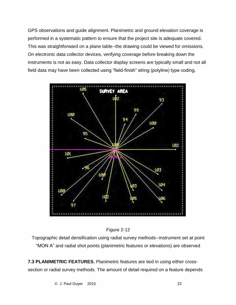
7.2 RADIAL SURVEY METHODS. (Figure 2-12). Plane tables were especially suited to

radial survey methods; thus, most surveys using total stations or RTK now utilize this

technique. Radial observation are made with the instrument (total station or RTK base

station) set up over a single point that has full project area visibility (or in the case of

RTK, can encompass radio or cell phone ranges well beyond visible limitations with a

total station). Thus, topographic features, baseline stakeout, and elevations be surveyed

without having to occupy separate stations along a fixed baseline. COGO packages will

automatically compute radial distances and azimuths to linear or curved baseline

stations, and visually guide the stakeout process. RTK surveys methods are a unique

form of radial survey methods—RTK controller COGO packages are used to reduce


GPS observations and guide alignment. Planimetric and ground elevation coverage is

performed in a systematic pattern to ensure that the project site is adequate covered.

This was straightforward on a plane table--the drawing could be viewed for omissions.

On electronic data collector devices, verifying coverage before breaking down the

instruments is not as easy. Data collector display screens are typically small and not all

field data may have been collected using “field-finish” string (polyline) type coding.

Figure 2-12

Topographic detail densification using radial survey methods--instrument set at point

“MON A” and radial shot points (planimetric features or elevations) are observed

7.3 PLANIMETRIC FEATURES. Planimetric features are tied in using either cross-

section or radial survey methods. The amount of detail required on a feature depends


on the nature of the project and the size of the feature relative to the target scale. On

small-scale topographic mapping projects, a generic symbol may be used to represent a

feature; however, on a detailed drawing for this same project, the feature may be fully

dimensioned. An example would be a 3 ft x 5 ft catch basin: on a 1inch = 400 ft scale

map, this basin would be represented by a symbol at its center point but might be

surveyed in detail (all four corner points located) on a 1inch = 30 ft site plan.

7.4 TOPOGRAPHIC ELEVATIONS AND CONTOURS. A variety of survey methods are

used to develop the terrain model for a given project area. The technique employed is a

function of the type of survey equipment, the detail required, and specified elevation

accuracy. In addition, the technique may depend on whether traditional contours or a

digital terrain model (DTM) is required.

7.5 CONTOURS FROM CROSS-SECTIONS. Contours can be directly surveyed on the

ground or derived from a terrain model of spot elevations. When cross-section methods

are employed, even contour intercepts along the offsets can be set in the field using a

level rod. Alternatively, elevations can be taken at intervals along the cross-section

where changes in grade or breaklines occur, and contour intercepts interpolated over

the linear portions. If abrupt changes in grade (or breaks in grade) occur between

crosssection stations, then supplemental cross-sections may be needed to better

represent the terrain and provide more accurate cut/fill quantity takeoffs.

7.6 CONTOURS FROM RADIAL SURVEYS--SPOT ELEVATION MATRICES. It is

often more efficient to generate contours from a DTM based on spot elevations taken

over a project area. These surveys are normally done with a total station or RTK

system; however, older transit-stadia or plane table methods will also provide the same

result. The density of spot elevations is based on the desired contour interval and

terrain gradient. In some instances, an evenly spaced grid of spot elevations may be

specified (so-called "post" spacing). Flat areas require fewer spots to delineate the

feature. Breaklines in the terrain are separately surveyed to ensure the final terrain

model is correctly represented. Data points can be connected using triangular irregular


network (TIN) methods and contours generated directly from the TIN in various CADD

packages (MicroStation InRoads, AutoCAD, etc.). The generated DTM or TIN also

provides a capability to perform "surface-to-surface" volume computations.

7.7 DTM GENERATION FROM BREAKLINE SURVEY TECHNIQUE. The following

guidance is excerpted from the California Department of Transportation (CALTRANS)

Surveys Manual. It describes a technique used by CALTRANS to develop DTMs on

total station topographic surveys. A DTM is a representation of the surface of the earth

using a triangulated irregular network (TIN). The TIN models the surface with a series of

triangular planes. Each of the vertices of an individual triangle is a coordinated (x,y,z)

topographic data point. The triangles are formed from the data points by a computer

program which creates a seamless, triangulated surface without gaps or overlaps

between triangles. Triangles are created so that their sides do not cross breaklines.

Triangles on either side of breaklines have common sides along the breakline.

Breaklines define the points where slopes change in grade (the intersection of two

planes). Examples of breaklines are the crown of pavement, edge of pavement, edge of

shoulder, flow line, top of curb, back of sidewalk, toe of slope, top of cut, and top of

bank. Breaklines within existing highway rights of way are clearly defined, while

breaklines on natural ground are more difficult to determine. DTMs are created by

locating topographic data points that define breaklines and random spot elevation

points. The data points are collected at random intervals along longitudinal break lines

with observations spaced sufficiently close together to accurately define the profile of

the breakline. Like contours, break lines do not cross themselves or other break lines.

Cross-sections can be generated from the finished DTM for any given alignments.

Method: When creating field-generated DTMs, data points are gathered along DTM

breaklines, and randomly at spot elevation points, using the total station radial survey

method. This method is called a DTM breakline survey. Because the photogrammetric

method in most cases is more cost effective, gathering data for DTMs using field

methods should be limited to small areas or to provide supplemental information for

photogrammetrically determined DTMs. The number of breaklines actually surveyed

can be reduced for objects of a constant shape such as curbs. To do this, a standard


cross section for such objects is sketched and made part of the field notes. Field-

collected breaklines are identified by line numbers and type on the sketch along with

distances and changes in elevation between the breaklines. With this information in the

field notes, only selected breaklines need to be located in the field, while others are

generated in the office based on the standard cross section. Advantages of DTM

breakline surveys:

Safety of field crews is increased because need to continually cross traffic is

eliminated.

Observations at specific intervals (stations) are not required.

New sets of cross sections can be easily created for each alignment change.

DTM survey guidelines:

Remember to visualize the TIN that will be created to model the ground surface

and how breaklines control placement of triangles.

Use proper topo codes, point numbering, and line numbers.

Use a special terrain code (e.g., 701) for critical points between breaklines,

around drop

inlets and culverts, and on natural ground in relatively level areas.

Make a sketch of the area to be surveyed identifying breaklines by number.

Do not change breakline codes without creating a new line.

Take shots on breaklines at approximately 20 m intervals and at changes in

grade.

Locate data points at high points and low points and on a grid of approximately

20 m centers when the terrain cannot be defined by breaklines.

If ground around trees is uniform, tree locations may be used as DTM data points

by using a terrain code of 701.

Keep site distances to a length that will ensure that data point elevations meet

desired

accuracies.

Gather one extra line of terrain points 5 to 10 m outside the work limits.


Accuracy Standard: Data points located on paved surfaces or any engineering works

should be located within ±10 mm horizontally and ± 7 mm vertically. Data points on

original ground should be located within ± 30 mm horizontally and vertically.

Checking: Check data points by various means including reviewing the resultant DTM,

reviewing breaklines in profile, and locating some data points from more than one setup.

Products: The surveys branch is responsible for developing and delivering final,

checked engineering survey products, including DTMs, to the survey requestors.

Products can be tailored to the needs of the requestor whenever feasible, but normally

should be kept in digital form and include the following items:

Converted and adjusted existing record alignments, as requested. (CAiCE

project subdirectory)

Surveyed digital alignments of existing roadways and similar facilities. (CAiCE

project subdirectory)

CAiCE DTM surface files. (CAiCE project subdirectory)

2-D CADD MicroStation design files, .dgn format.

Hard copy topographic map with border, title block, labeled contours, and

planimetry.

File of all surveyed points with coordinates and descriptions. (CTMED, .rpt,

format)

7.8 UTILITY SURVEY DETAIL METHODS. It is important to locate all significant utility

facilities. Utilities are surveyed using either total station or RTK techniques. The

CALTRANS Surveys Manual recommends that accuracy specifications for utilities that

are data points located on paved surfaces or any engineering works should be located

within ±10 mm horizontally and ±7 mm vertically. Data points on original ground should

be located within ±30 mm horizontally and vertically. The following are lists of facilities

and critical points to be located for various utilities--as recommended in the CALTRANS

Surveys Manual.


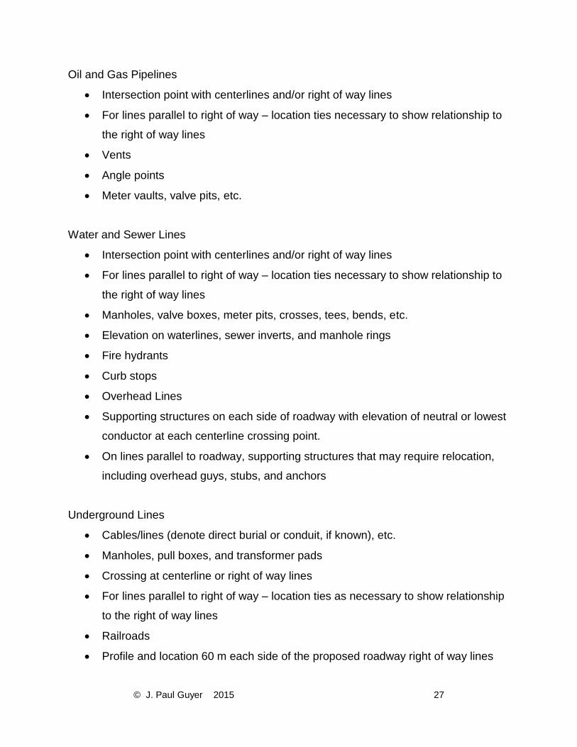
Oil and Gas Pipelines

Intersection point with centerlines and/or right of way lines

For lines parallel to right of way – location ties necessary to show relationship to

the right of way lines

Vents

Angle points

Meter vaults, valve pits, etc.

Water and Sewer Lines

Intersection point with centerlines and/or right of way lines

For lines parallel to right of way – location ties necessary to show relationship to

the right of way lines

Manholes, valve boxes, meter pits, crosses, tees, bends, etc.

Elevation on waterlines, sewer inverts, and manhole rings

Fire hydrants

Curb stops

Overhead Lines

Supporting structures on each side of roadway with elevation of neutral or lowest

conductor at each centerline crossing point.

On lines parallel to roadway, supporting structures that may require relocation,

including overhead guys, stubs, and anchors

Underground Lines

Cables/lines (denote direct burial or conduit, if known), etc.

Manholes, pull boxes, and transformer pads

Crossing at centerline or right of way lines

For lines parallel to right of way – location ties as necessary to show relationship

to the right of way lines

Railroads

Profile and location 60 m each side of the proposed roadway right of way lines


Switch points, signal, railroad facilities, communication line locations, etc.

Checking: Utility data should be checked by the following means:

Compare field collected data with existing utility maps

Compare field collected data with the project topo map/DTM

Review profiles of field collected data

Include field collected data, which have elevations, in project DTM

Locate some data points from more than one setup

7.9 ARCHAEOLOGICAL SITE/ENVIRONMENTALLY SENSITIVE AREA SURVEYS

(CALTRANS). Archaeological and environmental site surveys are performed for

planning and engineering studies. Surveys staff must work closely with the appropriate

specialists and the survey requestor to correctly identify archeological and

environmentally sensitive data points.

Method: Total station radial survey, GPS fast-static, kinematic, or RTK. Accuracy

Standard: Data points located on paved surfaces or engineering works should be

located within ±10 mm horizontally and ±7 mm vertically. Data points on original

grounds should be located within ±30 mm horizontally and vertically. Review field

survey package for possible higher required accuracy.

Checking: Check data points by various means including, reviewing the resultant DTM,

reviewing breaklines in profile, and locating some data points from more the one setup.

Products:

3-D digital graphic file of mapped area

Hard copy topographic map with border, title block, and planimetry (contours and

elevations only if specifically requested)

File of all surveyed points with coordinates and descriptions


7.10 SPOT LOCATION OR MONITORING SURVEYS (CALTRANS). Monitoring

surveys are undertaken for monitoring wells, bore hole sites, and other needs.

Method: Total station radial survey, GPS fast static or kinematic


should be located within ±10 mm horizontally and ±7 mm vertically. Data points on

original ground should be located within ±30 mm horizontally and vertically.

Checking: Observe data points with multiple ties.

Products:


Sketch or map showing locations of data points

7.11 VERTICAL CLEARANCE SURVEYS (CALTRANS). Vertical clearance surveys

are undertaken to measure vertical clearances for signs, overhead wires, and bridges.

Method: Total station radial method.


should be located within ±10 mm horizontally and ±7 mm vertically. Data points on

original ground should be located within ±30 mm horizontally and vertically.

Checking: Observe data points with multiple ties.

Products:


Sketch or map showing vertical clearances

Documents

An Introduction to Survey Methods and Techniques Methods and Techniques . An ... are not covered in this discussion but may be found in ... topographic points are measured by stadia