An Introduction to SaTScan Software to measure spatial,

temporal or space-time clusters using a spatial scan approach

Marilyn O’Hara University of Illinois moruiz@illinois.edu Lecture for the Pre-conference workshop ASCHP 11 Dec 2012

SaTScan Overview •  Developed by Martin Kulldorff with funding from National

Cancer Institute, CDC and other Agencies •  It is free and can be downloaded at

http://www.satscan.org •  New version (v. 9.0) came out Mar 2011 •  Used widely in public health and other fields to identify

high or low clusters of illness or other events across space and time.

What is a spatial scan? •  A circle (or ellipse) of varying sizes (from 0 –

upper distance set by user) systematically goes across (scans) the study area as it defines a dynamic geographic unit, or “moving window”.

•  In a typical situation, each original geographic unit (county, census tract, etc) is a potential cluster center.

•  Clusters are reported for those circles where observed values are greater than expected values. They can be at any location and be of varying sizes.

What about time? •  The condition of the event at varying temporal

periods is incorporated into the space-time scan. •  Think of it as a set of cylinders, of varying height

(for different time periods) that also scan spatially

•  Each time period can be the temporal start point of a space/time cluster. The number of different time periods (length of time) in clusters varies.

•  Space-time cluster is reported as spatial location, spatial size and the time period.

•  Temporal scan without space is also available.

For space-time cluster measure, each location is evaluated at a set of circles (or ellipses) of varying sizes. Each time period is evaluated alone as well as with the neighboring periods for each of the spatial sizes.

Day 1

Day 2

Day 3

Day 4

Day 5

Day 1

Day 2

Day 3

Day 4

Day 5

Location 1 Location 2

Clusters defined by radius, time period, and center point

2004

Mosquito Infection space-time clusters using a space-time permutation Poisson model in SaTScan.

Probability models for discrete (fixed location) scan statistics

•  Count data –  discrete Poisson (fastest to run; unlimited covariates; can

include population) –  Bernoulli (case/no case) –  space-time permutation (unlimited covariates; requires only

case data) •  Nominal/Ordinal data

–  ordinal (slowest to run; cases in ordered groups) –  multinomial (cases are in groups, with order e.g. severity of

illness, or nominal, e.g. serotype) •  Continuous

–  normal (can take positive or negative values) –  Exponential (designed for survival time analysis)

A few other things •  You can also use a continuous Poisson model to

determine if the events of interest have a spatial pattern, themselves, rather than if values (case counts, etc) have patterns

•  Some of the different model types give the same results in some situations. Some have more options so might be better choices.

•  To identify clusters, a likelihood function is maximized across all locations/times. The maximum likelihood indicates the cluster least likely to have occurred by chance = Cluster 1.

•  Clusters can be statistically significant or not. The p-value is obtained through Monte Carlo hypothesis testing.

•  Secondary clusters are those that are in rank order after Cluster 1, by their likelihood ratio test statistic.

Example 1: Mostashari et al. 2003. Dead bird clusters as an early warning system for West Nile virus activity

•  WNV in NYC, dead bird data for prospective analysis to predict human illness.

•  Bernoulli model, with census tracts •  As control, used record of prior,

unclustered, dead bird counts compared to dead birds in current time period.

•  Identified bird clusters as warning of increased risk for human illness.

Results- Example 1 Each census tract is either part or not part of a cluster.

Shading is based on number of clusters in tract up to date of map.

Example 2: Joly et al. 2006. Spatial epidemiology of Chronic Wasting Disease in Wisconsin white-tailed deer •  Tested if prevalence of CWD in Wisconsin

deer was uniform across study area •  Used Poisson model •  Cases of diseased deer per square mile

grid area •  The core affected area was identified from

the scan and prevalence measured inside that area compared to other areas

Results- Example 2 Circle indicates the single cluster in area (spatial only scan)

Shading is prevalence of CWD by square mile.

•  Measured spatial clustering of cleft palate/lip

•  Used geocoded birth records to count cases at several spatial scales (0.01 deg square grids, zipcode)

•  Used Bernoulli clustering with cases and controls per square grid.

•  Most of analysis was of incidence at zipcode level, not SaTScan.

Example 3: Cech et al. 2007. Orofacial cleft defect births and low-level radioactivity in tap water.

Results - Example 3 High case area was identified. Link between the high cases area and radioactivity in tap water was in analysis discussion.

•  Identify risk areas for malaria within villages for targeted control

•  Created grid of each village and counted households with cases for which treatment was sought

•  Used Bernoulli method for space-only scan of cases at household level.

•  Used retrospective space-time permutation on cases

Example 4: Coleman et al. 2009. Using the SaTScan method to detect local malaria clusters for guiding malaria control programmes.

Results- Example 4 Spatial clustersclusters in 4 of 7 villages.

Space time clusters in 2 of 7 (maps on right)

One secondary cluster identified

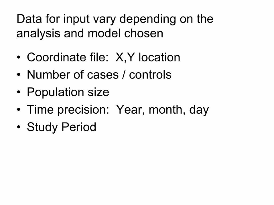
Data for input vary depending on the analysis and model chosen

•  Coordinate file: X,Y location •  Number of cases / controls •  Population size •  Time precision: Year, month, day •  Study Period

The output by SatScan

•  Results file – summary of results •  Cluster information – each row has data

for each cluster •  Location information - each row lists a

location and its cluster membership •  Risk estimates for each location •  Simulated log likelihood ratios

What SaTScan can and can’t do

•  CAN •  Identify spatial, temporal, spatio-temporal

patterns to find clusters in many types of data •  Provide flexible geographic units/neighborhoods •  Create output that can be read into GIS or other

programs •  CANNOT •  Process data for input

–  need SAS, SPSS, Excel, etc •  Display maps of events and cluster locations –

–  need GIS or mapping system •  Create other statistical models, e.g regression

models

Mostashari F, Kulldorff M, Hartman J J, Miller J R, Kulasekera V. Dead bird clusters as an early warning system for West Nile virus activity. Emerg Infect Dis 2003; (9): 641-646. Joly D O, Samuel M D, Langenberg J A, Blanchong J A, Batha C A, Rolley R E, Keane D P, Ribic C A. Spatial epidemiology of chronic wasting disease in Wisconsin white-tailed deer. J Wildl Dis 2006; (42): 578-588. Cech I, Burau K D, Walston J. Spatial distribution of orofacial cleft defect births in Harris County, Texas, 1990 to 1994, and historical evidence for the presence of low-level radioactivity in tap water. South Med J 2007; (100): 560-569. Coleman M, Coleman M, Mabuza A M, Kok G, Coetzee M, Durrheim D N. Using the SaTScan method to detect local malaria clusters for guiding malaria control programmes. Malar J 2009; (8): 68.