Embed Size (px)
Citation preview

AN INTRODUCTION TO QED & QCD By Dr G Zanderighi University of Oxford Lecture notes by Prof N Evans University of Southampton Lecture delivered at the School for Experimental High Energy Physics Students Somerville College, Oxford, September 2009
- 51 -

�
- 52 -

Contents
1 Introduction .............................................................................................. 55 1.1 Relativity Review...................................................................................... 56
2 Relativistic Wave Equations .................................................................. 58 2.1 The Klein-Gordon Equation .................................................................... 59 2.2 The Dirac Equation ................................................................................... 62 2.3 Solutions to the Dirac Equation .............................................................. 63 2.4 Orthogonality and Completeness........................................................... 65 2.5 Spin ............................................................................................................. 66 2.6 Lorentz Covariance................................................................................... 68 2.7 Parity, charge conjugation and time reversal ....................................... 71 2.8 Bilinear Covariants ................................................................................... 74 2.9 Massless (Ultra-relativistic) Fermions ................................................... 75
3 Quantum Electrodynamics..................................................................... 77 3.1 Classical Electromagnetism..................................................................... 77 3.2 The Dirac Equation in an Electromagnetic Field.................................. 79 3.3 g – 2 of the Electron................................................................................... 80 3.4 Interactions in Perturbation Theory....................................................... 82 3.5 Internal Fermions and External Photons............................................... 84 3.6 Summary of Feynman Rules for QED ................................................... 86
4 Cross Sections and Decay Rates............................................................ 88 4.1 Transition Rate .......................................................................................... 88 4.2 Decay Rates................................................................................................ 90 4.3 Cross Sections ............................................................................................ 91 4.4 Mandelstam Variables.............................................................................. 92
5 Processes in QED and QCD................................................................... 93 5.1 Electron-Muon Scattering ........................................................................ 93 5.2 Electron-Electron Scattering .................................................................... 95 5.3 Electron-Positron Annihilation............................................................... 96 5.4 Compton Scattering.................................................................................. 98 5.5 QCD Processes .......................................................................................... 99
6 Introduction to Renormalization ........................................................ 101 6.1 Ultraviolet (UV) Singularities ............................................................... 101 6.2 Infrared (IR) Singularities ...................................................................... 102 6.3 Renormalization...................................................................................... 102 6.4 Regularization ......................................................................................... 105
7 QED as a Field Theory .......................................................................... 107 7.1 Quantizing the Dirac Field .................................................................... 107 7.2 Quantizing the Electromagnetic Field ................................................. 109
Acknowledgements ............................................................................................. 112
References.............................................................................................................. 112
Pre-School Problems ........................................................................................... 113 Rotations, Angular Momentum and the Pauli Matrices............................. 113 Four Vectors ...................................................................................................... 113 Probability Density and Current Density ..................................................... 114
- 53 -

�
- 54 -

1 Introduction
The aim of this course is to teach you how to calculate transition amplitudes, crosssections and decay rates, for elementary particles in the highly successful theories ofQuantum Electrodynamics (QED) and Quantum Chromodynamics (QCD). Most of ourwork will be in understanding how to compute in QED. By the end of the course youshould be able to go from a Feynman diagram, such as the one for e−e− → μ−μ− infigure 5, to a number for the cross section. To do this we will have to learn how tocope with relativistic, quantum, particles and anti-particles that carry spin. In fact allthese properties of particles will emerge rather neatly from thinking about relativisticquantum mechanics. The rules for calculating in QCD are slightly more complicatedthat in QED, as we will briefly review, however, the basic techniques for the calculationare very similar.
We have a lot to cover so will necessarily have to take some short cuts. Our mainfudge will be to work in relativistic quantum mechanics rather than the full QuantumField Theory (QFT) (sometimes referred to as ‘second quantization’). We will be ingood company though since we will largely follow methods from Feynman’s papers andtext books such as Halzen and Martin. In quantum mechanics a classical wave is used todescribe a particle whose motion is subject to the Uncertainty Principle. In a full QFTthe wave’s motion itself is subject to the Uncertainty Principle too - the quanta of thatfield are what we then refer to as particles. Luckily at lowest order in a perturbationtheory calculation one neglects the quantum nature of the field and the two theoriesgive the same answer. At higher orders the quantum nature of the field gives rise tovirtual pair creation of particles - in the quantum mechanics version of the story theseare included in a more ad hoc fashion as we will see. Luckily the simultaneous QFTcourse will give you a good grounding in more precise methodologies.
Thus our starting point will be ordinary Quantum Mechanics and our first goal(section 2) will be to write down a ‘relativistic version’ of Quantum Mechanics. This willlead us to look at relativistic wave equations, in particular the Dirac equation, whichdescribes particles with spin 1/2. We will also develop a wave equation for photonsand look at how they couple to our fermions (section 3) - this is the core of QED. Aperturbation theory analysis will result in quantum mechanical probability amplitudesfor particular processes. After this, we will work out how to go from the probabilityamplitudes to cross sections and decay rates (section 4). We will look at some examples oftree level QED processes. Here you will get hands-on experience of calculating transitionamplitudes and getting from them to cross sections (section 5). We will restrict ourselvesto calculations at tree level but, at the end of the course (section 6), we will also take afirst look at higher order loop effects, which, amongst other things, are responsible forthe running of the couplings. For QCD, this running means that the coupling appearsweaker when measured at higher energy scales and is the reason why we can sometimesdo perturbative QCD calculations. However, in higher order calculations divergencesappear and we have to understand — at least in principle — how these divergences canbe removed.
In reference [1] you will find a list of textbooks that may be useful.
- 55 -

1.1 Relativity Review
An event in a reference frame S is described by the four coordinates of a four-vector (inunits where c = 1)
xμ = (t, �x), (1.1)
where the Greek index μ ∈ {0, 1, 2, 3}. These coordinates are reference frame dependent.The coordinates in another frame S ′ are given by x′μ, related to those in S by a LorentzTransformation (LT)
xμ → x′μ = Λμνx
ν , (1.2)
where summation over repeated indices is understood. This transformation identifies xμ
as a contravariant 4-vector (often referred to simply as a vector). A familiar example ofa LT is a boost along the z-axis, for which
Λμν =
⎛⎜⎜⎜⎝γ 0 0 −βγ0 1 0 00 0 1 0
−βγ 0 0 γ
⎞⎟⎟⎟⎠ , (1.3)
with, as usual, β = v and γ = (1 − β2)−1/2. LT’s can be thought of as generalizedrotations.
The “length” of the 4-vector (t2 − |�x|2) is invariant to LTs. In general we define theMinkowski scalar product of two 4-vectors x and y as
x · y ≡ xμyνgμν ≡ xμyμ, (1.4)
where the metric
gμν = gμν = diag(1,−1,−1,−1), gμλgλν = gμν = δμν ={
1 if μ = ν0 if μ �= ν
, (1.5)
has been introduced. The last step in eq. (1.4) is the definition of a covariant 4-vector(sometimes referred to as a co-vector),
xμ ≡ gμνxν . (1.6)
This transforms under a LT according to
xμ → x′μ = Λ ν
μ xν . (1.7)
Note that the invariance of the scalar product implies
ΛTgΛ = g ⇒ gΛTg = Λ−1, (1.8)
i.e. a generalization of the orthogonality property of the rotation matrix RT = R−1.
�Exercise 1.1Show eq. (1.8), starting from the invariance of the scalar product.
- 56 -

To formulate a coherent relativistic theory of dynamics we define kinematic variablesthat are also 4-vectors (i.e. transform according to eq. (1.2)). For example, we define a4-velocity
uμ =dxμ
dτ, (1.9)
where τ is the proper time measured by a clock moving with the particle. Everyonewill agree what the clock says at a particular event so this measure of time is Lorentzinvariant and uμ transforms as xμ. Note
uμ =dt
dτ
dxμ
dt= γ(1,�v) (1.10)
and has invariant lengthuμuμ = γ2(12 − |�v|2) = 1. (1.11)
Similarly 4-momentum provides a relativistic definition of energy and momentum
pμ = muμ ≡ (E, �p). (1.12)
The invariant length provides the crucial relation
pμpμ = E2 − |�p|2 = m2. (1.13)
�Exercise 1.2Check that dt/dτ = γ and that our relativistic definitions of E and �p make sense in thenon-relativistic limit.
The differentiation operator,
∂μ ≡ ∂
∂xμ=
(∂
∂t, �∇
), ∂μx
ν = δνμ, (1.14)
is a covariant 4-vector (i.e. according to eq. (1.7)). This means that the contravariantequivalent 4-vector will have an extra minus sign in its space-like components,
∂μ = (∂
∂t,−�∇). (1.15)
The convention for the totally antisymmetric Levi-Civita tensor is
εμνλσ =
⎧⎨⎩+1 if {μ, ν, λ, σ} an even permutation of {0, 1, 2, 3}−1 if an odd permutation0 otherwise
. (1.16)
Note that εμνλσ = −εμνλσ, and εμνλσpμqνrλsσ changes sign under a parity transformationsince it contains an odd number of spatial components.
�Exercise 1.3Verify the above two properties of εμνλσ.
I will use natural units, c = 1, h = 1, so mass, energy, inverse length and inverse timeall have the same dimensions. Generally think of energy as the basic unit, e.g. mass hasunits of GeV and distance has units of GeV−1.
�Exercise 1.4Noting that E has SI unit kg.m2.s−2, c has SI unit m.s−1 and h has SI unit kg.m2.s−1,what is a mass of 1 GeV in kg and what is a cross-section of 1 GeV−2 in microbarns?
- 57 -
2 Relativistic Wave Equations
Let’s review how wave equations describe non-relativistic quantum particles. Experimen-tally we know that a particle with definite momentum �p and energy E can be associatedwith a plane wave
ψ = ei(�k.�x−wt), with �k =�p
h, w =
E
h. (2.1)
To extract E and �p from the wave we use operators
Eψ = ihd
dtψ, �pψ = −ih�∇ψ. (2.2)
In quantum mechanics, it is more usual to refer to the energy operator as the HamiltonianH , and write (with h = 1)
Hψ = i∂ψ
∂t. (2.3)
I shall usually reserve the Greek symbol ψ for spin 1/2 fermions and φ for spin 0 bosons.So for pions and the like I shall write
Hφ = i∂φ
∂t. (2.4)
In non-relativistic systems, conservation of energy can be written
H = T + V, (2.5)
where T is the kinetic energy and V is the potential energy. A particle of mass m andmomentum �p has non-relativistic kinetic energy,
T =�p 2
2m. (2.6)
Replacing the energy and momentum operators with the forms seen in eq. (2.2), wearrive at the Schrodinger equation
ihd
dtψ = − h2
2m∇2ψ + V ψ. (2.7)
In this equation ψ is the wave function describing the single particle probability ampli-tude. For a slow moving particle v � c (e.g. an electron in a Hydrogen atom) this isadequate, but for relativistic systems (v ∼ c) the Hamiltonian above is incorrect.
For a free relativistic particle the total energy E is given by the Einstein equation
E2 = �p 2 + m2. (2.8)
Thus the square of the relativistic Hamiltonian H2 is simply given by promoting themomentum to operator status:
H2 = �p 2 + m2. (2.9)
So far, so good, but how should this be implemented into the wave equation of eq. (2.3),which is expressed in terms of H rather than H2? Naively the relativistic wave equationlooks like √
�p 2 + m2ψ(t) = i∂ψ(t)
∂t(2.10)
but this is difficult to interpret because of the square root. There are two ways forward:
- 58 -

1. Work with H2. By iterating the wave equation we have
H2φ(t) = −∂2φ(t)
∂t2
[or
(i∂
∂t− V
)2
φ(t)]
(2.11)
This is known as the Klein-Gordon (KG) equation. In this case the wave functiondescribes spinless bosons.
2. Invent a new Hamiltonian HD that is linear in momentum, and whose square isequal to H2 given above, H2
D = �p 2 + m2. In this case we have
HDψ(t) = i∂ψ(t)
∂t(2.12)
which is known as the Dirac equation, with HD being the Dirac Hamiltonian. Inthis case the wave function describes spin 1/2 fermions, as we shall see.
2.1 The Klein-Gordon Equation
Let us now take a more detailed look at the KG equation (2.11). In position space wewrite the energy-momentum operator as
pμ → i∂μ, (2.13)
so that the KG equation (for zero potential V ) becomes
(∂2 + m2) φ(x) = 0 (2.14)
where we recall the notation,
∂2 = ∂μ∂μ = ∂2/∂t2 −∇2 (2.15)
and x is the 4-vector (t, �x).The operator ∂2 is Lorentz invariant, so the Klein-Gordon equation is relativistically
covariant (that is, transforms into an equation of the same form) if φ is a scalar function.That is to say, under a Lorentz transformation (t, �x) → (t′, �x′),
φ(t, �x) → φ′(t′, �x′) = φ(t, �x) (2.16)
so φ is invariant. In particular φ is then invariant under spatial rotations so it representsa spin-zero particle (more on spin when we come to the Dirac equation); there being nopreferred direction which could carry information on a spin orientation.
The Klein-Gordon equation has plane wave solutions:
φ(x) = Ne−i(Et−�p·�x) (2.17)
where N is a normalization constant and E = ±√�p 2 + m2. Thus, there are both positive
and negative energy solutions. The negative energy solutions pose a severe problem if wetry to interpret φ as a wave function (as indeed we are trying to do). The spectrum is nolonger bounded from below, and we can extract arbitrarily large amounts of energy from
- 59 -

the system by driving it to ever more negative energy states. Any external perturbationcapable of pushing a particle across the energy gap of 2m between the positive andnegative energy continuum of states can uncover this difficulty. Furthermore, we cannotjust throw away these solutions as unphysical since they appear as Fourier modes in anyrealistic solution of (2.14). Note that if one interprets φ as a quantum field there is noproblem, as you will see in the field theory course. The positive and negative energymodes are just associated with operators which create or destroy particles.
A second problem with the wave function interpretation arises when trying to find aprobability density. Since φ is Lorentz invariant, |φ|2 does not transform like a density(i.e. as the time component of a 4-vector) so we will not have a Lorentz covariant con-
tinuity equation ∂ρ + �∇ · �J = 0. To search for a candidate we derive such a continuityequation. Defining ρ and �J by
ρ ≡ i
(φ∗∂φ
∂t− φ
∂φ∗
∂t
),
[or φ∗
(i∂
∂t− V
)+ φ
(−i
∂
∂t− V
)φ∗
], (2.18)
�J ≡ −i (φ∗�∇φ − φ�∇φ∗), (2.19)
we obtain (see problem) a covariant conservation equation
∂μJμ = 0, (2.20)
where J is the 4-vector (ρ, �J). It is thus natural to interpret ρ as a probability density
and �J as a probability current. However, for a plane wave solution (2.17), ρ = 2|N |2E,so the negative energy solutions also have a negative probability!
�Exercise 2.5Derive the continuity equation (2.20). Start with the Klein-Gordon equation multipliedby φ∗ and subtract the complex conjugate of the KG equation multiplied by φ.
Thus, ρ may well be considered as the density of a conserved quantity (such as elec-tric charge), but we cannot use it for a probability density. To Dirac, this and theexistence of negative energy solutions seemed so overwhelming that he was led to intro-duce another equation, first order in time derivatives but still Lorentz covariant, hopingthat the similarity to Schrodinger’s equation would allow a probability interpretation.Dirac’s original hopes were unfounded because his new equation turned out to admitnegative energy solutions too! Even so, he did find the equation for spin-1/2 particlesand predicted the existence of antiparticles.
Before turning to discuss what Dirac did, let us put things in context. We have foundthat the Klein-Gordon equation, a candidate for describing the quantum mechanics ofspinless particles, admits unacceptable negative energy states when φ is interpreted asthe single particle wave function. We could solve all our problems here and now, andrestore our faith in the Klein-Gordon equation, by simply re-interpreting φ as a quantumfield. However we will not do that. There is another way forward (this is the way followedin the textbook of Halzen & Martin) due to Feynman and Stuckelberg. Causality forcesus to ensure that positive energy states propagate forwards in time, but if we force thenegative energy states to propagate only backwards in time then we find a theory thatis consistent with the requirements of causality and that has none of the aforementioned
- 60 -

problems. In fact, the negative energy states cause us problems only so long as wethink of them as real physical states propagating forwards in time. Therefore, we shouldinterpret the emission (absorption) of a negative energy particle with momentum pμ asthe absorption (emission) of a positive energy antiparticle with momentum −pμ.
In order to become more familiar with this picture, consider a process with a π+ anda photon in the initial state and final state. In figure 1(a) the π+ starts from the pointA and at a later time t1 emits a photon at the point �x1. If the energy of the π+ is stillpositive, it travels on forwards in time and eventually will absorb the initial state photonat t2 at the point �x2. The final state is then again a photon and a (positive energy) π+.
There is another process however, with the same initial and final state, shown infigure 1(b). Again, the π+ starts from the point A and at a later time t2 emits a photonat the point �x1. But this time, the energy of the photon emitted is bigger than the energyof the initial π+. Thus, the energy of the π+ becomes negative and it is forced to travelbackwards in time. Then at an earlier time t1 it absorbs the initial state photon at thepoint �x2, thereby rendering its energy positive again. From there, it travels forward intime and the final state is the same as in figure 1(a), namely a photon and a (positiveenergy) π+.
time
spac
e
A
B
(t1, �x1)
(t2, �x2)
(a)
A
B
(t2, �x1)
(t1, �x2)
(b)
Figure 1: Interpretation of negative energy states
In todays language, the process in figure 1(b) would be described as follows: in theinitial state we have an π+ and a photon. At time t1 and at the point �x2 the photoncreates an π+π− pair. Both propagate forwards in time. The π+ ends up in the finalstate, whereas the π− is annihilated at (a later) time t2 at the point �x1 by the initialstate π+, thereby producing the final state photon. To someone observing in real time,the negative energy state moving backwards in time looks to all intents and purposeslike a negatively charged pion with positive energy moving forwards in time.
�Exercise 2.6Consider a wave incident on the potential step shown in figure 2. Show that if thestep size V > m + Ep, where Ep =
√�p2 + m2 then one cannot avoid using the negative
square root �k = −√
(Ep − V )2 + m2, resulting in negative currents and densities. Hint:
use the continuity of φ(x) and ∂φ(x)/∂x at x = 0, and ensure that the group velocityvg = ∂E/∂k is positive for x > 0. Interpret the solution.
- 61 -

a exp(i�p · �x) d exp(i�k · �x)
b exp(−i�p · �x)
V
x = 0
Figure 2: A potential step
2.2 The Dirac Equation
Dirac wanted an equation first order in time derivatives and Lorentz covariant, so ithad to be first order in spatial derivatives too. His starting point was to assume aHamiltonian of the form,
HD = α1p1 + α2p2 + α3p3 + βm, (2.21)
where pi are the three components of the momentum operator �p, and αi and β aresome unknown quantities, which we will show must be interpreted as 4 × 4 matrices.Substituting the expressions for the operators eq. (2.13) into the Dirac Hamiltonian ofeq. (2.21) results in the equation
i∂ψ
∂t= (−i �α · �∇ + βm)ψ (2.22)
which is the position space Dirac equation.If ψ is to describe a free particle it must satisfy the Klein-Gordon equation so that
it has the correct energy-momentum relation. This requirement imposes relationshipsamong α1, α2, α3 and β. To see this, apply the Hamiltonian operator to ψ twice, to give
−∂2ψ
∂t2= [−αiαj∇i∇j − i (βαi + αiβ)m∇i + β2m2]ψ, (2.23)
with an implicit sum of i and j over 1 to 3. The Klein-Gordon equation by comparisonis
−∂2ψ
∂t2= [−∇i∇i + m2]ψ. (2.24)
It is clear that we cannot recover the KG equation from the Dirac equation if the αi andβ are normal numbers. Insisting that the terms linear in ∇i vanish independently wouldrequire either β to vanish or all the αi to vanish. This would remove either ∇i∇j termor the m2 term, both of which are unacceptable. Instead we must insist that the termslinear in ∇i vanish in their sum without any of αi or β vanishing, i.e. we must assumethat αi and β anti-commute. We recover the KG equation only if
αiαj + αjαi = 2δij
- 62 -

βαi + αiβ = 0 (2.25)
β2 = 1
for i, j = 1, 2, 3. In principle, these equations define αi and β, and any objects whichobey these relations are good representations of them. However, in practice, we willrepresent them by matrices. In this case, ψ is a multi-component spinor on which thesematrices act.
�Exercise 2.7Prove that any matrices �α and β satisfying eq. (2.25) are traceless with eigenvalues ±1.Hence argue that they must be even dimensional.
In two dimensions a natural set of matrices for the �α would be the Pauli matrices
σ1 =(
0 11 0
), σ2 =
(0 −ii 0
), σ3 =
(1 00 −1
). (2.26)
However, there is no other independent 2 × 2 matrix with the right properties for β, sowe must use a higher dimensional form. The smallest number of dimensions for whichthe Dirac matrices can be realized is four. One choice is the Dirac representation:
�α =(
0 �σ�σ 0
), β =
(1 00 −1
). (2.27)
Note that each entry above denotes a two-by-two block and that the 1 denotes the 2× 2identity matrix. The spinor ψ therefore has four components.
There is a theorem due to Pauli that states that all sets of matrices obeying therelations in eq. (2.25) are equivalent. Since the hermitian conjugates �α† and β† clearlyobey the relations, you can, by a change of basis if necessary, assume that �α and β arehermitian. All the common choices of basis have this property. Furthermore, we wouldlike αi and β to be hermitian so that the Dirac Hamiltonian (2.42) is hermitian.
If we defineρ = J0 = ψ†ψ, �J = ψ†�αψ, (2.28)
then it is a simple exercise using the Dirac equation to show that this satisfies thecontinuity equation ∂μJ
μ = 0. We will see in section 2.8 that (ρ, �J) transforms, as itmust, as a 4-vector. Note that ρ is now also positive definite.
2.3 Solutions to the Dirac Equation
We look for plane wave solutions of the form
ψ =(χ(�p)φ(�p)
)e−i(Et−�p·�x) (2.29)
where φ(�p) and χ(�p) are two-component spinors that depend on momentum �p but areindependent of �x. Using the Dirac representation of the matrices, and inserting the trialsolution into the Dirac equation gives the pair of simultaneous equations
E(χφ
)=
(m �σ · �p�σ · �p −m
) (χφ
). (2.30)
There are two simple cases for which eq. (2.30) can readily be solved, namely
- 63 -

1. �p = 0, m �= 0, which might represent an electron in its rest frame.
2. m = 0, �p �= 0, which describes a massless particle or a particle in the ultra-relativistic limit (E � m).
For case (1), an electron in its rest frame, the equations (2.30) decouple and becomesimply,
Eχ = mχ, Eφ = −mφ. (2.31)
So, in this case, we see that χ corresponds to solutions with E = m, while φ correspondsto solutions with E = −m. In light of our earlier discussions, we no longer need to recoilin horror at the appearance of these negative energy states.
The negative energy solutions persist for an electron with �p �= 0 for which the solutionsto equation (2.30) are
φ =�σ · �pE+m
χ, χ =�σ · �pE−m
φ. (2.32)
�Exercise 2.8Show that (�σ · �p)2 = �p2.
Using (�σ · �p)2 = �p2 we see that E = ±|√�p 2 + m2|. We write the positive energysolutions with E = +|√�p 2 + m2| as
ψ(x) =(
χ�σ·�pE+m
χ
)e−i(Et−�p·�x), (2.33)
while the general negative energy solutions with E = −|√�p 2 + m2| are
ψ(x) =( �σ·�p
E−mφ
φ
)e−i(Et−�p·�x), (2.34)
for arbitrary constant φ and χ. Clearly when �p = 0 these solutions reduce to the positiveand negative energy solutions discussed previously.
It is interesting to see how Dirac coped with the negative energy states. Dirac inter-preted the negative energy solutions by postulating the existence of a “sea” of negativeenergy states. The vacuum or ground state has all the negative energy states full. Anadditional electron must now occupy a positive energy state since the Pauli exclusionprinciple forbids it from falling into one of the filled negative energy states. On promot-ing one of these negative energy states to a positive energy one, by supplying energy, anelectron-hole pair is created, i.e. a positive energy electron and a hole in the negativeenergy sea. The hole is seen in nature as a positive energy positron. This was a radicalnew idea, and brought pair creation and antiparticles into physics. The problem withDirac’s hole theory is that it does not work for bosons. Such particles have no exclusionprinciple to stop them falling into the negative energy states, releasing their energy.
It is convenient to rewrite the solutions, eqs. (2.33) and (2.34), introducing the spinorsu (s)α (�p) and v (s)
α (�p). The label α ∈ {1, 2, 3, 4} is a spinor index that often will be sup-pressed, while s ∈ {1, 2} denotes the spin state of the fermion, as we shall see later. Wetake the positive energy solution eq. (2.33) and define
√E+m
(χs
�σ·�pE+m
χs
)e−ip·x ≡ u(s)(p)e−ip·x. (2.35)
- 64 -
For the negative energy solution of eq. (2.34), change the sign of the energy, E → −E,and the three-momentum, �p → −�p, to obtain,
√E+m
( �σ·�pE+m
χsχs
)eip·x ≡ v(s)(p)eip·x. (2.36)
In these two solutions E is now (and for the rest of the course) always positive and givenby E = (�p 2 + m2)1/2. The χs for s = 1, 2 are
χ1 =(
10
), χ2 =
(01
). (2.37)
For the simple case �p = 0 we may interpret χ1 as the spin-up state and χ2 as thespin-down state. Thus for �p = 0 the 4-component wave function has a very simpleinterpretation: the first two components describe electrons with spin-up and spin-down,while the second two components describe positrons with spin-up and spin-down. Thuswe understand on physical grounds why the wave function had to have four components.The general case �p �= 0 is slightly more involved and is considered in the next section.
The u-spinor solutions will correspond to particles and the v-spinor solutions toantiparticles. The role of the two χ’s will become clear in the following section, where itwill be shown that the two choices of s are spin labels. Note that each spinor solutiondepends on the three-momentum �p, so it is implicit that p0 = E.
2.4 Orthogonality and Completeness
Our solutions to the Dirac equation take the form
ψ = Nu(s)e−ip.x, ψ = Nv(r)eip.x, with r, s = 1, 2, (2.38)
where N is a normalization factor. We have already included a factor√
E+m in ourspinors (see eqs. (2.35) and (2.36)), which results in
u(r) †(p)u(s)(p) = v(r) †(p)v(s)(p) = 2Eδrs. (2.39)
This convention allows u†u to transform as the time component of a 4-vector underLorentz transformations, which is essential to its interpretation as a probability density(see eq. (2.28) and section 2.8). Also note that the spinors are orthogonal.
�Exercise 2.9Check the normalization condition for the spinors in eq. (2.39).
We must further normalize the spatial part of the wave functions. In fact a planewave is not normalizable in an infinite space so in the computatuions that follow wherewe use them we will work in a large box of volume V - such a construction is not Lorentzinvariant. The number of particles in the box will be∫
ψ†ψ d3x = 2E N2 V, (2.40)
so setting N = 1/√
V allows us to adopt the standard relativistic normalization con-vention of 2E particles per box of volume V . Most people and the books use this
- 65 -

convention. I frequently find it more intuitive, given we’ve broken Lorentz invariance, toset N = 1/
√2EV so there’s one particle in the box. I’ll try to be clear below when I do
this.Remember that the solutions to the wave equation form a complete set of states
meaning that we can expand (like a Fourier expansion) an arbitrary function χ(x) interms of them
χ(x) =∑n
anψn(x) (2.41)
The an are the equivalent of Fourier coefficients and if χ is a wave function in somequantum mixed state then |an|2 is the probability of being in the state ψn (or 2E timesthat!).
2.5 Spin
Now it is time to justify the statements we have been making that the Dirac equationdescribes spin-1/2 particles. The Dirac Hamiltonian in momentum space is given ineq. (2.21) as
HD = �α · �p + βm, (2.42)
and the orbital angular momentum operator is
�L = �R× �p. (2.43)
Evaluating the commutator of �L with HD,
[�L, HD] = [�R× �p, �α · �p]
= [�R, �α · �p] × �p
= i�α × �p, (2.44)
we see that the orbital angular momentum is not conserved (otherwise the commutator
would be zero). We would like to find a total angular momentum �J that is conserved,
by adding an additional operator �S to �L,
�J = �L + �S, [ �J , HD] = 0. (2.45)
To this end, consider the three matrices,
�Σ ≡(�σ 00 �σ
)= −iα1α2α3�α, (2.46)
where the first equivalence is merely a definition of �Σ and the last equality can be verifiedby an explicit calculation. The �Σ/2 have the correct commutation relations to representangular momentum, since the Pauli matrices do, and their commutators with �α and βare,
[�Σ, β] = 0, [Σi, αj] = 2iεijkαk. (2.47)
- 66 -

From the relations in (2.47) we find that
[�Σ, HD] = −2i�α × �p. (2.48)
�Exercise 2.10Using α1α2α3 ≡ 1
3εijkαiαjαk verify the commutation relations in eqs. (2.47) and (2.48).
Comparing eq. (2.48) with the commutator of �L with HD in eq. (2.44), you see that
[�L +1
2�Σ, HD] = 0, (2.49)
and we can identify
�S =1
2�Σ (2.50)
as the additional quantity that, when added to �L in equation (2.45), yields a conserved
total angular momentum �J . We interpret �S as an angular momentum intrinsic to theparticle. Now
�S2 =1
4
(�σ · �σ 0
0 �σ · �σ)
=3
4
(1 00 1
), (2.51)
and, recalling that the eigenvalue of �J 2 for spin j is j(j+1), we conclude that �S representsspin-1/2 and the solutions of the Dirac equation have spin-1/2 as promised. We workedin the Dirac representation of the matrices for convenience, but the result is necessarilyindependent of the representation.
Now consider the u-spinor solutions u(s)(p) of eq. (2.35). Choose �p = (0, 0, pz) andwrite
u↑ ≡ u(1)(p) =
⎛⎜⎜⎜⎝√
E+m0√
E−m0
⎞⎟⎟⎟⎠ , u↓ ≡ u(2)(p) =
⎛⎜⎜⎜⎝0√
E+m0
−√E−m
⎞⎟⎟⎟⎠ . (2.52)
With these definitions, we get
Szu↑ =1
2u↑, Szu↓ = −1
2u↓. (2.53)
So, these two spinors represent spin up and spin down along the z-axis respectively. Forthe v-spinors, with the same choice for �p, write,
v↓ = v(1)(p) =
⎛⎜⎜⎜⎝√
E−m0√
E+m0
⎞⎟⎟⎟⎠ , v↑ = v(2)(p) =
⎛⎜⎜⎜⎝0
−√E−m0√
E+m
⎞⎟⎟⎟⎠ , (2.54)
where now,
Szv↓ =1
2v↓, Szv↑ = −1
2v↑. (2.55)
This apparently perverse choice of up and down for the v’s is actually quite sensiblewhen one realizes that a negative energy electron carrying spin +1/2 backwards in timelooks just like a positive energy positron carrying spin −1/2 forwards in time.
- 67 -

2.6 Lorentz Covariance
There is a much more compact way of writing the Dirac equation, which requires thatwe get to grips with some more notation. Define the γ-matrices,
γ0 = β, �γ = β�α. (2.56)
In the Dirac representation,
γ0 =(
1 00 −1
), �γ =
(0 �σ−�σ 0
). (2.57)
In terms of these, the relations between the �α and β in eq. (2.25) can be written compactlyas,
{γμ, γν} = 2gμν . (2.58)
�Exercise 2.11Prove that {γμ, γν} = 2gμν.
Combinations like aμγμ occur frequently and are conventionally written as,
/a = aμγμ = aμγμ,
pronounced “a slash.” Note that γμ is not, despite appearances, a 4-vector. It justdenotes a set of four matrices. However, the notation is deliberately suggestive, for whencombined with Dirac fields you can construct quantities that transform like vectors andother Lorentz tensors (see the next section).
Observe that using the γ-matrices the Dirac equation (2.22) becomes
(i/∂ − m)ψ = 0, (2.59)
or, in momentum space,(/p − m)ψ = 0. (2.60)
The spinors u and v satisfy
(/p − m)u(s)(p) = 0, (2.61)
(/p + m)v(s)(p) = 0, (2.62)
since for v(s)(p), E → −E and �p → −�p.We want the Dirac equation (2.59) to preserve its form under Lorentz transformations
eq. (1.2). We’ve just naively written the matrices in the Dirac equation as γμ howeverthis does not make them a 4-vector! They are just a set of numbers in four matricesand there’s no reason they should change when we do a boost. Since ∂μ does transform,for the equation to be Lorentz covariant we are led to propose that ψ transforms too.We know that 4-vectors get their components mixed up by LT’s, so we expect that thecomponents of ψ might get mixed up too:
ψ(x) → ψ′(x′) = S(Λ)ψ(x) = S(Λ)ψ(Λ−1x′) (2.63)
- 68 -

where S(Λ) is a 4 × 4 matrix acting on the spinor index of ψ. Note that the argumentΛ−1x′ is just a fancy way of writing x, i.e. each component of ψ(x) is transformed intoa linear combination of components of ψ(x).
In order to appreciate the above it is useful to consider a vector field, where thecorresponding transformation is
Aμ(x) → A′μ(x′)
where x′ = Λx. This makes sense physically if one thinks of space rotations of a vectorfield. For example the wind arrows on a weather map are an example of a vector field:with each point on the map there is associated an arrow. Consider the wind directionat a particular point on the map, say Abingdon. If the map is rotated, then one wouldexpect on physical grounds that the wind vector at Abingdon always point in the samephysical direction and have the same length. In order to achieve this, both the vectoritself must rotate, and the point to which it is attached (Abingdon) must be correctlyidentified after the rotation. Thus the vector at the point x′ (corresponding to Abingdonin the rotated frame) is equal to the vector at the point x (corresponding to Abingdonin the unrotated frame), but rotated so as to keep the physical sense of the vector thesame in the rotated frame (so that the wind always blows towards Oxford, say, in thetwo frames). Thus having correctly identified the same point in the two frames all weneed to do is rotate the vector:
A′μ(x′) = ΛμνA
ν(x). (2.64)
A similar thing also happens in the case of the 4-component spinor field above, exceptthat we do not (yet) know how the components of the wave function themselves musttransform, i.e. we do not know S.
We now need to figure out what S is. The requirement is that the Dirac equationhas the same form in any inertial frame. Thus, if we make a LT from our original frameinto another (‘primed’) frame and write down the Dirac equation in this frame, it has tohave the same form.
(iγμ∂μ − m)ψ(x) = 0 −→ (iγμ∂′μ − m)ψ′(x′) = 0, (2.65)
where we used the fact that m is a scalar, i.e. m′ = m.The derivative transforms as a covector, eq. (1.7), so using the orthogonality condition
of eq. (1.8), we can write ∂μ = Λσμ∂
′σ and multiplying the Dirac equation in the original
frame by S it becomesS(iγμΛσ
μ∂′σ − m)ψ(x) = 0. (2.66)
On the other hand, we can use the definition of S in eq. (2.63) to rewrite the equationin the primed frame as
(iγμ∂′μ − m)Sψ(x) = 0. (2.67)
We can see that the second term (containing m) of eqs. (2.66) and (2.67) are nowidentical. To make the first term identical we need SΛσ
μγμ = γσS. Thus, in order for
the Dirac equation to be Lorentz invariant, S(Λ) has to satisfy
Λσμγ
μ = S−1γσS (2.68)
- 69 -

We still haven’t solved for S explicitly. We need to find an S that satisfies eq. (2.68).Since S depends on the LT, we first have to find a convenient parameterization of a LTand then express S(Λ) in terms of these parameters. For an infinitesimal LT, it can beshown that,
Λμν = gμν + ωμ
ν (2.69)
where ωμν is an antisymmetric set of infinitesimal parameters. For example, a boostalong the z-axis corresponds to ω03 = −ω30 = −β (remember that ω0i = ω0
i = −ω0i etc)
with all other entries of ωμν zero,
Λμν = gμν + ωμ
ν =
⎛⎜⎜⎜⎝1 0 0 −β0 1 0 00 0 1 0−β 0 0 1
⎞⎟⎟⎟⎠ . (2.70)
This corresponds to eq. (1.3) when one makes an expansion in small β, i.e. γ = 1 +O(β2). Non-zero ω01 or ω02 correspond to boosts along the x and y axes respectively.The remaining combinations, non-zero ω23, ω31 or ω12, correspond to infinitesimal anti-clockwise rotations through an angle ωij about the x, y and z axes respectively. It’s anice exercise to check this out.
For an infinitesimal LT we are at liberty to write
S(Λ) = 1 +i
4ωμνσ
μν , (2.71)
which is nothing but a definition of the set of matrices σμν . Our task is to determinethese matrices. To do this, substitute the expression for S, eq. (2.71), into eq. (2.68) (andremember that S−1(Λ) = 1 − i
4ωμνσ
μν). After some algebra, we can convince ourselvesthat the solution is
σμν =i
2[γμ, γν ] (2.72)
Thus S can be written explicitly in terms of γ-matrices for a general LT by building thefinite transformation out of lots of infinitesimal ones.
�Exercise 2.12Verify that eq. (2.72) is true.
Now that we now how ψ transforms we can find quantities that are Lorentz invariant,or transform as vectors or tensors under LT’s. To this end, we will find it useful tointroduce the Dirac adjoint. The Dirac adjoint ψ of a spinor ψ is defined by
ψ ≡ ψ†γ0 (2.73)
With the help ofS†(Λ)γ0 = γ0S−1(Λ) (2.74)
we see that ψ transforms under LT’s as
ψ → ψ ′ = ψS−1(Λ). (2.75)
�Exercise 2.13
- 70 -

1. Verify that γμ† = γ0γμγ0.
2. Prove eq. (2.74)
3. Show that ψ satisfies the equation
ψ (−i←/∂ − m) = 0
where the arrow over /∂ implies the derivative acts to the left.
4. Hence prove that ψ transforms as in eq. (2.75).
Combining the transformation properties of ψ and ψ in eqs. (2.63) and (2.75) we seethat the bilinear ψψ is Lorentz invariant. In section 2.8 we will consider the transforma-tion properties of general bilinears.
Let’s close this section by recasting the spinor normalization eq. (2.39) in terms ofDirac inner products. The conditions become
u(r)(p)u(s)(p) = 2mδrs
u(r)(p)v(s)(p) = v(r)(p)u(s)(p) = 0 (2.76)
v(r)(p)v(s)(p) = −2mδrs
where, in analogy to eq. (2.73), we defined u ≡ u†γ0 and v ≡ v†γ0.
�Exercise 2.14Verify the normalization properties in the above equations (2.76).
2.7 Parity, charge conjugation and time reversal
2.7.1 Parity
We usually use LT’s which are in the connected Lorentz Group, SO(3, 1), meaning theycan be obtained by a continuous deformation of the identity transformation (i.e. by lotsof little transformations)1. This class of LT is often referred to as proper LT. However,the full Lorentz group consists not only of the proper transformations but also includesthe discrete operations of parity (space inversion), P , and time reversal, T :
ΛP =
⎛⎜⎜⎜⎝1 0 0 00 −1 0 00 0 −1 00 0 0 −1
⎞⎟⎟⎟⎠ , ΛT =
⎛⎜⎜⎜⎝−1 0 0 0
0 1 0 00 0 1 00 0 0 1
⎞⎟⎟⎟⎠ . (2.77)
LT’s satisfy ΛTgΛ = g, so taking determinants shows that det Λ = ±1. Proper LT’s arecontinuously connected to the identity so must have determinant 1, but both P and Toperations have determinant −1.
Let us now find the action of parity on the Dirac wave function and determine thewave function ψP in the parity-reversed system. According to the discussion of theprevious section, we need to find a matrix P satisfying
P−1γ0P = γ0, P−1γiP = −γi. (2.78)
1Indeed in the last section we considered LT’s very close to the identity in equation (2.69)
- 71 -
Using some properties of the γ-matrices we see that P = P−1 = γ0 is an acceptablesolution (Clearly one could multiply γ0 by a phase and still have an acceptable definitionfor the parity transformation.), from which it follows that the transformation is
ψ(t, �x) → ψP (t,−�x) = Pψ(t, �x) = γ0ψ(t, �x). (2.79)
Since
γ0 =(
1 00 −1
), (2.80)
the u-spinors and v-spinors at rest have opposite eigenvalues, corresponding to particleand antiparticle having opposite intrinsic parities.
2.7.2 Charge Conjugation
Another discrete invariance of the Dirac equation is charge conjugation, which takes youfrom particle to antiparticle and vice versa. For scalar fields the symmetry is just complexconjugation, but in order for the charge conjugate Dirac field to remain a solution ofthe Dirac equation, you have to mix its components as well. The transformation on thefermion wavefunction is
ψ → ψC = Cψ T , (2.81)
where ψ T =(ψ†γ0
)T= γ0Tψ†T = γ0ψ∗. To find the form of C, let’s take the complex
conjugate of the Dirac Equation,
(iγμ∂μ − m)∗ ψ∗ =(i(γμ †)T ∂μ − m
) (ψ†)T
= γ0T(−iγμ T∂μ − m
)ψT , (2.82)
where we have additionally used γμ † = γ0γμγ0. Premultiply by C and the Dirac equationbecomes (
−iCγμ TC−1∂μ − m)
ψc = 0. (2.83)
In order for ψC to satisfy the Dirac equation we require C to be a matrix satisfying thecondition
CγTμC−1 = −γμ (C−1 = C†). (2.84)
In the Dirac representation,a suitable choice for this operator is
C = iγ2γ0 =(
0 −iσ2
−iσ2 0
). (2.85)
The charge-conjugation transformation is then
ψ(t, �x) → ψC(t, �x) = CψT (t, �x) = iγ2γ0ψT (t, �x). (2.86)
When Dirac wrote down his equation everybody thought parity and charge conju-gation were exact symmetries of nature, so invariance under these transformations wasessential. Now we know that neither of them, nor the combination CP , is respected bythe standard electroweak model.
- 72 -

2.7.3 Time reversal
As already noted, time reversal is an improper LT, given by ΛT in eq. (2.77). Naivelyone would expect to derive a time reversal operation in the same way as for parity.However, there is a subtlety that the momentum of a particle is a rate of change, so if wereverse the direction of time, the momentum must change direction. When we reversethe momentum �p in a plane wave we find
e−i(Et−�p·�x) −→ e−i(Et−(−�p)·�x) = ei(E(−t)−�p·�x) =(e−i(E(−t)−�p·�x)
)∗. (2.87)
In this example, taking the complex conjugate is the equivalent of reversing the timecoordinate and reversing the momentum. So once again, we must take the complexconjugate of the field, transforming it according to
ψ(t, �x) → ψT (−t, �x) = Tψ∗(t, �x). (2.88)
To find the form of T , let’s take the complex conjugate of the Dirac equation, premultiplyby T and interchange t → −t,(
iγ0 ∂
∂t+ i�γ · �∇− m
)ψ(t, �x) −→ ST
(−iγ0 ∗ ∂
∂(−t)− i�γ∗ · �∇− m
)T−1Tψ∗(−t, �x)
=
(i[Tγ0 ∗T−1
] ∂
∂t+ i
[−T�γ∗T−1
]· �∇− m
)ψT (t, �x).
(2.89)
For ψT to satisfy the Dirac equation we need
i[Tγ0 ∗T−1
]= γ0,
[−T�γ∗T−1
]= −�γ. (2.90)
A suitable choice is
T = iγ1γ3 =
(0 −iσ1σ3
−iσ1σ3 0
)= i
⎛⎜⎜⎜⎝0 1 0 0−1 0 0 00 0 0 10 0 −1 0
⎞⎟⎟⎟⎠ , (2.91)
and the time reversal transformation on a fermion field is
ψ(t, �x) → ψT (−t, �x) = Tψ∗(t, �x) = iγ1γ3ψ∗(t, �x) (2.92)
2.7.4 CPT
We are now in the position to ask what is the effect of performing charge conjugation,parity and time-reversal all together on a Dirac field. The combined transformation isknown as CPT. Using eqs. (2.79), (2.86) and (2.92), the CPT transformation is,
ψ(t, �x) → ψCPT (−t,−�x) = iγ2γ0γ0T[γ0iγ1γ3ψ∗(t, �x)
]∗= iγ2γ0γ0γ0(−i)γ1γ3ψ(t, �x)
= γ0γ1γ2γ3ψ(t, �x)
= −iγ5ψ(t, �x) (2.93)
- 73 -

Thus, apart from the factor of γ5, a particle moving forward in time is equivalent to ananti-particle moving backwards in time and in the opposite direction. In fact, the extraγ5 makes no difference to observable quantities (see the next section) so this justifies theFeynman-Stuckelberg interpretation of negative energy states we used earlier.
2.8 Bilinear Covariants
Now, as promised, we will construct and classify the bilinears. These are useful for defin-ing quantities with particular properties under Lorentz transformations, and appearingin Lagrangians for fermion field theories.
To begin, note that by forming products of the γ-matrices it is possible to construct 16linearly independent 4×4 matrices. Any constant 4×4 matrix can then be decomposedinto a sum over these basis matrices. In equation (2.72) we have defined
σμν ≡ i
2[γμ, γν ],
and now it is convenient to define
γ5 ≡ γ5 ≡ iγ0γ1γ2γ3 =(
0 11 0
), (2.94)
where the last equality is valid in the Dirac representation. This new matrix satisfies
γ5† = γ5,{γ5, γμ
}= 0, (γ5)2 = 1. (2.95)
�Exercise 2.15Prove the three results in eq. (2.95) independently of the γ-matrix representation.
Now, the set of 16 matrices {1, γ5, γμ, γμγ5, σμν
}form a basis for γ-matrix products. There are 16 matrices since there is 1 unit matrix,1 γ5 matrix, 4 γμ matrices and 4 γμγ5 matrices, and 6 σμν matrices (see equation (2.72)for the definition of σμν).
Using the transformations of ψ and ψ from eqs. (2.63) and (2.75), together with thetransformation of γμ in eq. (2.74), the 16 fermion bilinears and their transformationproperties can be written as follows:
ψψ → ψψ S scalar
ψγ5ψ → det(Λ) ψγ5ψ P pseudoscalar
ψγμψ → Λμνψγ
νψ V vector
ψγμγ5ψ → det(Λ) Λμνψγ
νγ5ψ A axial vector
ψσμνψ → ΛμλΛ
νσψσ
λσψ T tensor (2.96)
In particular we note that
ψγμψ = ψ†γ0γμψ = (ψ†ψ, ψ†�αψ) (2.97)
which is our previous definition eq. (2.28) of the current 4–vector Jμ, i.e. we now seethat it is really a 4–vector.
- 74 -

�Exercise 2.16Derive the transformation properties of the bilinears in equation (2.96) under C, P, Tand CPT transformations.
2.9 Massless (Ultra-relativistic) Fermions
At very high energies we may neglect the masses of particles (E2 � |�p|2). Therefore, letus look at solutions of the Dirac equation with m = 0, on the basis that this will be anextremely good approximation for many situations.
From equation (2.30) we have in this case
Eφ = �σ · �pχ, Eχ = �σ · �p φ. (2.98)
These equations can easily be decoupled by taking linear combinations and defining thetwo component spinors ΨL and ΨR,
ΨR/L ≡ χ± φ
2, (2.99)
which leads toEΨR = �σ · �pΨR, EΨL = −�σ · �p ΨL. (2.100)
The system is in fact described by two entirely separated two component spinors. If wetake them to be moving in the z direction, and noting that σ3 = diag(1,−1), we see thatthere is one positive and one negative energy solution in each.
Further since E = |�p| for massless particles, these equations may be written
�σ · �p|�p| ΨL = −ΨL,
�σ · �p|�p| ΨR = ΨR (2.101)
Now, 12�σ·�p|�p| is known as the helicity operator (i.e. it is the spin operator projected in the
direction of motion of the momentum of the particle). We see that the ΨL corresponds tosolutions with negative helicity, while ΨR corresponds to solutions with positive helicity.In other words ΨL describes a left-handed particle while ΨR describes a right-handedparticle, and each type is described by a two-component spinor.
The two-component spinors transform very simply under LT’s,
ΨL → ei2�σ.(�θ−i�φ)ΨL (2.102)
ΨR → ei2�σ.(�θ+i�φ)ΨR (2.103)
where �θ = �nθ corresponds to space rotations through an angle θ about the unit �naxis, and �φ = �vφ corresponds to Lorentz boosts along the unit vector �v with a speedv = tanhφ. Note that these transformations are consistent with the fact that it is notpossible to boost past a massless particle (i.e. its helicity cannot be reversed).
However, under parity transformations �σ → �σ (like �R × �p), �p → −�p, therefore�σ · �p → −�σ · �p, i.e. the spinors transform into each other:
ΨL ↔ ΨR. (2.104)
- 75 -

So a theory in which ΨL has different interactions to ΨR (such as the standard model inwhich the weak force only acts on left handed particles) manifestly violates parity.
Although massless particles can be described very simply using two componentspinors as above, they may also be incorporated into the four-component formalismby using the γ5 we defined earlier. Let’s define projection operators
PR/L ≡ 1
2
(1 ± γ5
). (2.105)
In the Dirac representation, these are,
PR/L =1
2
(1 ±1
±1 1
), (2.106)
where 1 denotes the 2×2 identity matrix. Acting these projection operators on a generalDirac field of the form eq. (2.29) projects onto right- or left-handed eigenstates. To seethis, first note that
PR/L
(χφ
)=
1
2
(1 ±1
±1 1
) (χφ
)=
(ΨR/L
ΨR/L
). (2.107)
The helicity operator in four-component Dirac space is given by �S · �p/|�p|, with �S = 12�Σ,
where �Σ is defined in equation (2.46). Acting this operator on the projected state gives
1
2
⎛⎝ �σ·�p|�p| 0
0 �σ·�p|�p|
⎞⎠ (ΨR/L
ΨR/L
)= ±1
2
(ΨR/L
ΨR/L
), (2.108)
indicating that the projected states are indeed right- or left-handed eigenstates withhelicity ±1
2.
This can be made more explicit by using a different representation for the γ-matrices.In the chiral representation (sometimes called the Weyl representation) we define the γ-matrices to be
γ0 ≡(
0 11 0
), �γ ≡
(0 �σ�σ 0
), (2.109)
so that, with γ5 = iγ0γ1γ2γ3 as before, the projection operators eq. (2.105) become
PR =
(0 00 1
), PL =
(1 00 0
). (2.110)
Now, the left-handed Weyl spinor sits in the upper two components of the Dirac spinor,while the right-handed Weyl spinor sits in the lower two components of the Dirac spinor.The projection operators pick out only the upper or lower component, e.g.
PR
(ΨL
ΨR
)=
(0 00 1
) (ΨL
ΨR
)=
(0
ΨR
), (2.111)
so the projected states are once again helicity eigenstates.
- 76 -

3 Quantum Electrodynamics
3.1 Classical Electromagnetism
So far, we have only considered relativistic wave equations for free particles. Now we wantto include electromagnetic interactions, so let’s start by reviewing Maxwell’s Equationsin differential form:
�∇. �E = ρ, �∇. �B = 0,
�∇× �E = −∂ �B
∂t, �∇× �B = �J +
∂ �E
∂t.
(3.1)
Note here that I’m using Heaviside Lorentz units - I’ve used my freedom to choose theunit of charge to set ε0 = 1. Then, since in natural units c = 1, μ0 = 1 too. Whenone plays these games the value of the electron charge changes but the dimensionlessquantity α = e2/4πε0hc remains unchanged - α = 1/137.
We can rewrite the Maxwell equations in terms of a scalar potential φ, and a vectorpotential �A. Writing
�E = −∂ �A
∂t− �∇φ,
�B = �∇× �A,
(3.2)
we automatically have solutions of two of the Maxwell equations,
�∇. �B = �∇.(�∇× �A) ≡ 0 (3.3)
and
�∇× �E = �∇×⎛⎝−∂ �A
∂t− �∇φ
⎞⎠
= −∂(�∇× �A)
∂t− �∇× (�∇φ)
= −∂ �B
∂t.
(3.4)
This simplifies things greatly since now there are only two Maxwell equations to solve.
Let’s write them out in terms of the potentials,
�∇. �E = −∇2φ − d(�∇. �A)
dt= ρ, (3.5)
and (since �∇× �∇× �A ≡ −∇2 �A + �∇.(�∇. �A)),
�∇(�∇. �A) −∇2 �A = �J +∂
∂t
⎛⎝−∂ �A
∂t− �∇φ
⎞⎠ . (3.6)
- 77 -

or rearranging,
−∇2 �A +∂2 �A
∂t2= �J − �∇(�∇. �A +
∂φ
∂t). (3.7)
Unfortunately these two equations we are left with are quite complicated. To simplifythem up we note that we can redefine our potentials,
�A → �A + �∇ψ,
φ → φ − ∂ψ
∂t, (3.8)
without changing �E and �B. This redefinition of the potentials is known as a gaugetransformation.
�Exercise 3.17Check that �E and �B are invariant under the gauge transformation in eq. (3.8).
We can choose a gauge transformation such that
�∇. �A = −∂φ
∂t. (3.9)
In this gauge (the Lorentz gauge) Maxwell’s equations simplify to
−∇2φ +∂2φ
∂t2= ρ, (3.10)
−∇2 �A +∂2 �A
∂t2= �J . (3.11)
As well as being prettier, these equations also have a very suggestive form. They suggestwe should define the 4-vectors,
Jμ = (ρ, �J), Aμ = (φ, �A), (3.12)
so the Maxwell equations may be written in a manifestly covariant form,
∂2Aμ = Jμ. (3.13)
The μ = 0 equation is the φ eq. (3.10) and the μ = 1, 2, 3 equations give the components
of the eq. (3.11) for �A. The gauge condition, eq. (3.9), becomes
∂μAμ = 0. (3.14)
Eq. (3.13) is the classical wave equation for the electromagnetic field. In free spacewe have eq. (3.13) with no source, i.e.
∂2Aμ = 0, (3.15)
which has plane wave solutions,Aμ = εμeiq.x, (3.16)
- 78 -

where εμ is the polarization tensor and q2 = 0.The Lorentz condition, eq. (3.14), enforces
qμεμ = 0, (3.17)
which removes one degree of freedom. Even after enforcing this condition, there is stillroom to make more gauge transformations,
Aμ → Aμ + ∂μχ where ∂2χ = 0. (3.18)
This can be used to remove one extra degree of freedom from εμ. There are thereforetwo physical degrees of freedom, the normal polarizations of a photon.
3.2 The Dirac Equation in an Electromagnetic Field
We will now treat Aμ as a quantum mechanical wave function for photons. In the limitof a large number of photons the wave function is interpreted as a number density andproduces the classical wave theory. But so far we have no interactions; to allow electronsto interact with electromagnetism we have to include the photon field into our Diracequation.
The ’obvious’ thing to do is to just be led by Lorentz invariance. The field Aμ is avector field so we need to ’soak up’ its free index with a γ-matrix. We therefore includeit into the Dirac equation as
(iγμ∂μ − eγμAμ − m) ψ = 0, (3.19)
where the factor of e is a free constant which quantifies how strongly the electron couplesto the photon (the charge of the electron is −e).
It is convenient to incorporate this extra term into a new definition of a covariantderivative2,
Dμ ≡ ∂μ + ieAμ. (3.20)
Our interacting Dirac equation was therefore obtained from the free Dirac equation bythe minimal substitution ∂μ → Dμ, and the Dirac equation becomes
(i /D − m)ψ = 0. (3.21)
There is a much nicer and theoretically much more appealing way to get the interac-tion term. That is if we require the QED Lagrangian to be invariant under a local gaugesymmetry consisting of the transformations
ψ → e−ieΛ(x)ψ, Aμ → Aμ − ∂μΛ(x). (3.22)
then we are forced to the wave equation in eq. (3.21). For more details, I refer you tothe Standard Model course.
We must also allow the electrons to enter into the photon wave equation but here theclassical theory already tells us how a current density enters. We expect
∂2Aμ = Jμ (3.23)
where Jμ is just given by the charge times the Dirac equation number density (−eψγμψ).
2Conventions for the covariant derivative vary. Halzen and Martin, and Mandl and Shaw both useDμ ≡ ∂μ− ieAμ whereas Peskin and Schroeder both use eq. (3.20). Both conventions define the electroncharge to be −e but differ by a sign in the definition of the photon field, Aμ.
- 79 -

3.3 g − 2 of the Electron
We now have a wave equation which describes how an electron behaves in an electro-magnetic field, i.e. eq. (3.19). We will immediately put this to use by investigating theinteraction between the spin of a non-relativistic electron and a magnetic field.
Writing the electron field in the form of eq. (2.29), we see that eq. (3.19) gives(χφ
)=
(m �σ · (−i�∇− e �A)
�σ · (−i�∇− e �A) −m
) (χφ
)(3.24)
Substituting the equation from the second row into the that from the first leads to,⎛⎜⎝E − m +
[�σ · (−i�∇− e �A)
]2
E + m
⎞⎟⎠χ = 0. (3.25)
We can simplify this somewhat by using to relation
σiσj = δij + iεijkσk, (3.26)
to show [�σ ·
(−i�∇− e �A
)]2= | − i�∇− e �A|2 − e
(�∇× �A + �A × �∇
)· �σ, (3.27)
and note�∇× �A ψ + �A × �∇ψ =
(�∇× �A
)ψ = �Bψ. (3.28)
Putting all this together we find,⎛⎝E − m +|�p − e �A|2 − e �B · �σ
E + m
⎞⎠χ = 0. (3.29)
In the non-relativistic limit we can write E ≈ m and observe that the lower 2-componentspinor is
φ ≈ �σ · (�p − e �A)
2mχ � χ. (3.30)
This allows us to write, for the 4-component spinor ψ,
1
2m|�p − e �A|2ψ − e �B · �Σ
2mψ = 0. (3.31)
Notice that we have a coupling between the magnetic field �B and the spin of theelectron �S = 1
2�Σ. This is known as a magnetic moment interaction and takes the form
−�μ · �B. (3.32)
Our Dirac equation in an electromagnetic field has predicted
�μ = − e
2m�Σ. (3.33)
- 80 -

In classical physics the magnetic moment of an orbiting charge is written
�μorb = − e
2mc�L. (3.34)
This is the magnetic moment associated with orbital angular momentum. By analogywe define the magnetic moment due to intrinsic angular momentum (i.e. spin) as
�μspin = −ge
2m�S = −g
2
e
2m�Σ (3.35)
where g is the gyromagnetic ratio of the particle. The Dirac equation predicts
g = 2. (3.36)
Experimentally one finds for the electron that
g = 2.0023193043738± 0.0000000000082, (3.37)
so the Dirac equations prediction is pretty close. It is not exactly correct, as we can seefrom the incredible precision with which this quantity has been measured. The discrep-ancy is due to us not yet including quantum corrections to our prediction. The interactionof an electron with a photon (and thus the gyromagnetic ratio) will be changed by pro-cesses of the form seen in fig. 3, and processes involving yet more particle loops. When
Figure 3: Quantum corrections to the electron-photon interaction.
one performs a more careful analysis, including these quantum effects, one predicts thedeviation from 2 to be
g − 2
2= 1 +
α
2π− 0.328
(α
π
)2
+ 1.181(
α
π
)3
− 1.510(
α
π
)4
+ . . . + 4.393× 10⁻¹², (3.38)
and comparing this prediction with experiment:
Theory :g − 2
2= 1159652140(28)× 10−12,
Experiment :g − 2
2= 1159652186.9(4.1)× 10−12.
(3.39)
The figure in brackets denotes the error on the last significant figure. We can see thatthe experimental measurement matches the theoretical prediction to 8 significant figures,making this prediction of QED the most precisely tested prediction in physics.
- 81 -
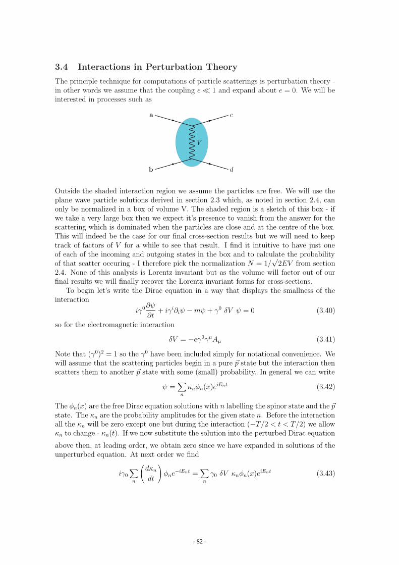
3.4 Interactions in Perturbation Theory
The principle technique for computations of particle scatterings is perturbation theory -in other words we assume that the coupling e � 1 and expand about e = 0. We will beinterested in processes such as
a
b
c
d
V
Outside the shaded interaction region we assume the particles are free. We will use theplane wave particle solutions derived in section 2.3 which, as noted in section 2.4, canonly be normalized in a box of volume V. The shaded region is a sketch of this box - ifwe take a very large box then we expect it’s presence to vanish from the answer for thescattering which is dominated when the particles are close and at the centre of the box.This will indeed be the case for our final cross-section results but we will need to keeptrack of factors of V for a while to see that result. I find it intuitive to have just oneof each of the incoming and outgoing states in the box and to calculate the probabilityof that scatter occuring - I therefore pick the normalization N = 1/
√2EV from section
2.4. None of this analysis is Lorentz invariant but as the volume will factor out of ourfinal results we will finally recover the Lorentz invariant forms for cross-sections.
To begin let’s write the Dirac equation in a way that displays the smallness of theinteraction
iγ0 ∂ψ
∂t+ iγi∂iψ − mψ + γ0 δV ψ = 0 (3.40)
so for the electromagnetic interaction
δV = −eγ0γμAμ (3.41)
Note that (γ0)2 = 1 so the γ0 have been included simply for notational convenience. Wewill assume that the scattering particles begin in a pure �p state but the interaction thenscatters them to another �p state with some (small) probability. In general we can write
ψ =∑n
κnφn(x)eiEnt (3.42)
The φn(x) are the free Dirac equation solutions with n labelling the spinor state and the �pstate. The κn are the probability amplitudes for the given state n. Before the interactionall the κn will be zero except one but during the interaction (−T/2 < t < T/2) we allowκn to change - κn(t). If we now substitute the solution into the perturbed Dirac equation
above then, at leading order, we obtain zero since we have expanded in solutions of theunperturbed equation. At next order we find
iγ0
∑n
(dκn
dt
)φne−iEnt =
∑n
γ0 δV κnφn(x)eiEnt (3.43)
- 82 -

Now we will make use of the orthogonality of the φn to extract the final state κn. Wemultiply through by
∫d3x φ†
fγ0
dκfdt
= −i∑n
κn
∫d3x φ†
fδV φn e−i(En−Ef )t (3.44)
For a discussion of normalization of the spinors see section 2.4. Remembering that att = −T/2 κi = 1 and κi=n = 0 at leading order we have
dκfdt
= −i∫
ψ†fδV ψi d3x (3.45)
and integrating with respect to t we find the important result
κf (T/2) = −i∫
ψ†fδV ψi d4x (3.46)
Now lets use our explicit form for δV in QED and concentrate on the scattering of aparticle a → c by a photon Aμ
a c
κca = −i∫
ψc(−eγμAμ)ψa d4x
= −i∫Jcaμ Aμ d4x
(3.47)
whereJcaμ = −e ψcγμψ
a = −e NaNc ucγμu
a ei(pc−pa).x (3.48)
The Ns here are the normalizations of the spatial wave functions ψ again from section2.5.
We’re really interested in two particles scattering off each other so we’d better com-pute the Aμ field produced when another particle scatters from state b → d
b d
�Aμ = Jμdb = −e NbNd udγμub ei(pd−pb).x (3.49)
the solution is
Aμ = − 1
q2Jμdb, q = pd − pb (3.50)
- 83 -

So finally substituting this back into our expression for κca we find
κfi = −i NaNbNcNd uc(−eγμ)u
a
(− 1
q2
)ud(−eγμ)ub
∫ei(pb+pd−pa−pc).xd4x (3.51)
Note that the integral is just a delta function that ensures 4-momentum conservation inthe interaction. In order to make this result more memorable Feynman developed his
famous rules that associate different parts of the expression with elements of a diagramof the scattering.
u
i g_ μ�
q 2
i e �μ
i e ��
u
u
u
a
b d
c�
_
where momentum is conserved at the vertices. Multipling these rules out gives us −iMfi
where
κfi = −i NaNbNcNd (2π)4δ4(pf − pi) Mfi (3.52)
�Exercise 3.18Derive the Feynman rules for the scattering of two particles described by the KleinGordon equation to leading order in e. You may Assume the form of the result in (3.46).
3.5 Internal Fermions and External Photons
We concentrated above on a scattering with external fermions interacting by the exchangeof a photon. We can also imagine processes where there are external photon fields orinternal virtual fermions. What are the Feynman rules for these cases? Given timeconstraints, rather than derive them, I’ll present some simple arguments to motivate therules. If we have an external photon interacting with a fermion in some way, then thevertex rule is still −ieγμ. Since the amplitude we wish to calculate is Lorentz invariant wecan not allow a stray μ index to survive but must soak it up with a 4-vector. The obvious4-vector associated with external photon is its polarization vector εμ and indeed this isthe appropriate factor for an external photon. Compare this to the way an externalfermion closes the gamma matrix space indicies, to give a number, with the externalspinor.
- 84 -

We have seen that an internal photon (satisfying �Aμ = 0) generates a Feynman rule(or propagator)
�Aμ = 0 → −igμνp2
(3.53)
Since a photon is just a collection of four scalar fields we can deduce that a massless,scalar field (which satisfies the KG equation �φ = 0) will have a Feynman rule
�φ = 0 → i
p2(3.54)
It turns out that the sign is that of a space-like photon degree of freedom. To find thepropagator of a massive scalar field we can treat the mass as a perturbing interaction ofthe free particle. Writing the KG equation as
�φ = −δV φ = −m2φ (3.55)
will generate a Feynman rule for the scalar self interaction
−im
Now we can consider the set of perturbation theory diagrams that contribute to the fullscalar propagator
+ + +ip2
ip2(−im) i
p2ip2(−im) i
p2(−im) ip2+ + +
i
p2→ i
p2+
i
p2(−im)
i
p2+
i
p2(−im)
i
p2(−im)
i
p2+ ... (3.56)
Pleasingly we can resum this series
i
p2
(1 +
m2
p2+
m4
p4+ ...
)=
i
p2
⎛⎝ 1
1 − m2
p2
⎞⎠ =i
p2 − m2(3.57)
and this is indeed the full propagator in the massive case. By this point we can see thatthe propagator is basically just −i times the inverse of the free field equation operatorin momentum space. A sensible guess for the fermionic field is
(i/∂ − m)ψ = 0 → i
/p − m=
i
/p − m
/p + m
/p + m=
i(/p + m)
p2 − m2(3.58)
This is in fact the correct answer. You will receive more insight into these results fromthe Field Theory course.
- 85 -

For every . . . draw . . . write . . .
Internal photon lineμ ν −igμν
p2 + i0+
Internal fermion lineα β
pi(/p + m)αβ
p2 − m2 + i0+
Vertex
α β
μ−ieγμαβ
Outgoing electron uα(s, p)
Incoming electron uα(s, p)
Outgoing positron vα(s, p)
Incoming positron vα(s, p)
Outgoing photon ε∗μ(λ, p)
Incoming photon εμ(λ, p)
• Attach a directed momentum to every internal line• Conserve momentum at every vertex, i.e. include δ(4)(
∑pi)
• Integrate over all internal momenta
Table 1: Feynman rules for QED. μ, ν are Lorentz indices, α, β are spinor indices ands and λ fix the polarization of the electron and photon respectively.
3.6 Summary of Feynman Rules of QED
The Feynman rules for computing the amplitude Mfi for an arbitrary process in QEDare summarized in Table 1.
The spinor indices in the Feynman rules are such that matrix multiplication is per-formed in the opposite order to that defining the flow of fermion number. The arrow onthe fermion line itself denotes the fermion number flow, not the direction of the momen-tum associated with the line: I will try always to indicate the momentum flow separatelyas in Table 1. This will become clear in the examples which follow. We have alreadymet the Dirac spinors u and v. I will say more about the photon polarization vector εwhen we need to use it.
To summarize, the procedure for calculating the amplitude for any process in QEDis the following:
1. Draw all possible distinct diagrams
2. Associate a directed 4-momentum with all lines
3. Apply the Feynman rules for the propagators, vertices and external legs
4. Ensure 4-momentum conservation at each vertex by adding (2π)4δ4(ki −kf ),whereki and kf are the total incoming and outgoing 4-momenta of the vertex respectively
- 86 -

5. Perform the integration over all internal momenta with the measure∫
d4k/(2π)4
It is also part of the Feynman rules for QED that when diagrams differ by an interchangeof two fermion lines, a relative minus sign must be included. This is a reflection of Pauli’sexclusion principle or equivalently of the anticommutation of the fermion operators dis-cussed in the appendix. Note, however, that you don’t need to get the absolute sign ofan amplitude right, just its sign relative to the other amplitudes, since it is the modulusof the amplitude squared that we need ultimately. This sounds rather complicated. Inparticular there seem to be an awful lot of integrations to be done. However, at tree-level,i.e. if there are no loop diagrams, the delta functions attached to the vertices togetherwith the integration over the internal momenta simply result in an overall 4-momentumconservation, i.e. in a factor (2π)4δ4(Pi − Pf), where Pi and Pf are the total incomingand outgoing 4-momenta of the process. Thus at tree-level, no ‘real’ integration has tobe done. At one loop, however, there is one non trivial integration to be done. Gen-erally, the calculation of an n-loop diagram involves n non trivial integrations. Evenworse, these integrals very often are divergent. Still, we can get perfectly reasonabletheoretical predictions at any order in QED. The procedure to get these results is calledrenormalization and will be the topic of section 6. At this point, some remarks con-cerning step 1, i.e. drawing all possible distinct Feynman diagrams, might be useful.In order to establish whether two diagrams are distinct, we have to try to convert oneinto the other. If this is possible without cutting lines and without gluing lines – thatis solely by twisting and stretching the lines and rotating the whole figure – then thetwo diagrams are identical. It should be noted that the external lines are labeled in thisprocess. Therefore, the two diagrams shown in figure 6 are different. Finally, let memention that the diagrams shown in figure 1 are not Feynman diagrams. When drawingFeynman diagrams we are only interested in what particles are incoming and which onesare outgoing and there is no time direction involved.
- 87 -

4 Cross Sections and Decay Rates
Before explicitly calculating some transition amlitudes lets see how to connect thoseamplitudes to physical observables such as cross sections and particle widths.
4.1 Transition Rate
Consider an arbitrary scattering process with an initial state i with total 4-momentum Pi
and a final state f with total 4-momentum Pf . Let’s assume we computed the scatteringamplitude for this process in QED, i.e. we know the matrix element
−iN∏f=1
Nf
∏in
Ni Mfi(2π)4δ4(Pf − Pi) (4.1)
Our task in this section is to convert this into a scattering cross section (relevant if thereis more than 1 particle in the initial state) or a decay rate (relevant if there is just 1particle in the initial state), see figure 4.
(a) (b)
Figure 4: Scattering (a) and decay (b) processes.
The probability for the transition to occur is the square of the matrix element, i.e.
Probability = | − iN∏f=1
Nf
∏in
Ni Mfi(2π)4δ4(Pf − Pi)|2. (4.2)
Attempting to take the squared modulus of the amplitude produces a meaningless squareof a delta function. This is a technical problem because our amplitude is expressedbetween plane wave states. These states are states of definite momentum and so extendthroughout all of space-time. In a real experiment the incoming and outgoing states arelocalized (e.g. they might leave tracks in a detector). To deal with this properly we wouldhave to construct normalized wave packet states which do become well separated in thefar past and the far future. A sloppier derivation is to maintain that our interaction isoccuring in a box of volume V = L3 and over a time of order T . The final answers willcome out independent of V and T , reproducing the ones we would get if we worked withlocalized wave packets. Using
(2π)4δ4(Pf − Pi) =∫
ei(Pf−Pi)x d4x (4.3)
we get in our space-time box the result
|(2π)4δ4(Pf − Pi)|2 � (2π)4δ4(Pf − Pi)∫
ei(Pf−Pi)x d4x � V T (2π)4δ4(Pf − Pi). (4.4)
- 88 -

We must also use the explicit expressions for the wave function normalizations fromsection 2.4. Above we used the normalization N = 1/
√2EV . So putting everything
together, we find for the transition rate W , i.e. the probability per unit time
W =1
T|Mfi|2V T (2π)4δ4(Pf − Pi)
N∏f=1
[1
2EfV
] ∏in
[1
2EiV
]. (4.5)
As expected, the dependence on T cancelled. Usually we are interested in much moredetailed information than just the total transition rate. We want to know the differentialtransition rate dW , i.e. the transition rate into a particular element of the final statephase space. To get dW we have to multiply by the number of available states in the(small) part of phase space under consideration. For a single particle final state, the
number of available states dn in some momentum range �k to �k + d�k is, in the boxnormalization,
dn = V d3�k (4.6)
This result is proved by recalling that the allowed momenta in the box have componentsthat can only take on discrete values such as kx = 2πnx/L where nx is an integer. Thusdn = dnxdnydnz and the result follows. For a two particle final state we have
dn = dn1dn2
wheredn1 = V d3�k1, dn2 = V d3�k2,
where dn is the number of final states in some momentum range �k1 to �k1+d�k1 for particle1 and �k2 to �k2 + d�k2 for particle 2. There is an obvious generalization to an N particlefinal state,
dn =N∏f=1
V d3�kf(2π)3
. (4.7)
The transition rate for transitions into a particular element of final state phase space isthus given by, using equations (4.7) and (4.5),
dW = |Mfi|2(2π)4δ4(Pf − Pi)VN∏f=1
[1
2EfV
] ∏in
[1
2EiV
] N∏f=1
V d3�kf(2π)3
= |Mfi|2V∏in
[1
2EiV
]× LIPS(N) , (4.8)
where in the second step we defined the Lorentz invariant phase space with N particlesin the final state
LIPS(N) ≡ (2π)4δ4(Pf − Pi)N∏f=1
d3�kf(2π)3 2Ef
. (4.9)
Observe that everything in the transition rate is Lorentz invariant save for the initialenergy factor and the factors of V .
�Exercise 4.19Show that d3k/2E is a Lorentz-invariant element of phase space. (Hint: Think how youwould write the phase space in a 4-dimensional, integral but with the particle on-shell,i.e. E = (�k2 + m2)1/2).
- 89 -

4.2 Decay Rates
We turn now to the special case where we have only one particle with mass m in theinitial state i, i.e. we consider the decay of this particle into some final state f . In thiscase, the transition rate is called the partial decay rate and denoted by Γif . First of all,we observe that the dependence on V cancels, as advertised above. In the rest frame ofthe particle the partial decay rate is given by
Γif =1
2m
∫|Mfi|2 × LIPS (4.10)
The important special case of two particles in the final state deserves further considera-tion. Consider the partial decay rate for a particle i of mass m into two particles f1 andf2. The Lorentz-invariant phase space is
LIPS(N) = (2π)4δ4(pi − p1 − p2)d3�p1
(2π)3 2E1
d3�p2
(2π)3 2E2. (4.11)
In the rest frame the four-vectors of each particle are
pi = (m, 0), p1 = (E1, �p), p2 = (E2,−�p). (4.12)
Therefore we can eliminate one three-momentum in the phase space
LIPS(N) =1
(2π)2δ(m − E1 − E2)
d3�p2
4E1E2. (4.13)
Hence the partial decay rate becomes
Γif =1
8m(2π)2
∫|Mfi|2δ(m − E1 − E2)
d|�pf |2|�pf |dΩ∗
E1E2(4.14)
where dΩ∗ is the solid angle element for the angle of one of the outgoing particles withrespect to some fixed direction, and �pf is the momentum of one of the final state particles.But from the on-shell condition E1 = (�p2
1 + m21)
1/2, we have dE1 = |�pf |/E1 d|�pf | andsimilarly for particle 2 and so
d(E1 + E2) = |�pf |d|�pf |E1 + E2
E1E2,
therefore
|�pf |2d|�pf | 1
E1E2
=|�pf |
E1 + E2
d(E1 + E2). (4.15)
Using this in eq. (4.14) and integrating over (E1 + E2) we obtain the final result
Γi→f1f2 =1
32π2m2
∫|Mfi|2|�pf |dΩ∗. (4.16)
The total decay rate of particle i is obtained by summation of the partial decay ratesinto all possible final states
Γtot =∑f
Γif (4.17)
- 90 -

The total decay rate is related to the mean life time τ via (Γtot)−1 = τ . For completeness
I also give the definition of the branching ratio for the decay into a specific final state f
Bf ≡ Γif
Γtot
(4.18)
In an arbitrary frame we find, W = (m/E)Γtot, which has the expected Lorentz dilationfactor. In the master formula (equation (4.8)) this is what the product of 1/2Ei factorsfor the initial particles does.
4.3 Cross Sections
The total cross section for a static target and a beam of incoming particles is defined asthe total transition rate for a single target particle and a unit beam flux. The differentialcross section is similarly related to the differential transition rate. We have calculatedthe differential transition rate with a choice of normalization corresponding to a single‘target’ particle in the box, and a ‘beam’ corresponding also to one particle in the box.A beam consisting of one particle per volume V with a velocity v has a flux N0 given by
N0 =v
V
particles per unit area per unit time. Thus the differential cross section is related to thedifferential transition rate in equation (4.8) by
dσ =dW
N0
= dW × V
v. (4.19)
Now let us generalize to the case where in the frame in which you make the measurements,the ‘beam’ has a velocity v1 but the ‘target’ particles are also moving with a velocity v2.In a colliding beam experiment, for example, v1 and v2 will point in opposite directionsin the laboratory. In this case the definition of the cross section is retained as above,but now the beam flux of particles N0 is effectively increased by the fact that the targetparticles are moving towards it. The effective flux in the laboratory in this case is givenby
N0 =|�v1 − �v2|
V
which is just the total number of particles per unit area which run past each other per unittime. I denote the velocities with arrows to remind you that they are vector velocities,which must be added using the vector law of velocity addition, not the relativistic law.In the general case, then, the differential cross section is given by
dσ =dW
N0=
1
|�v1 − �v2|1
4E1E2|Mfi|2 × LIPS (4.20)
where we have used equation (4.8) for the transition rate, and the box volume V hasagain canceled. The amplitude-squared and phase space factors are manifestly Lorentzinvariant. What about the initial velocity and energy factors? Observe that
E1E2(�v1 − �v2) = E2�p1 − E1�p2.
- 91 -

In a frame where �p1 and �p2 are collinear,
|E2�p1 − E1�p2|2 = (p1 · p2)2 − m2
1m22,
and the last expression is manifestly Lorentz invariant.
�Exercise 4.20Prove that |E2�p1−E1�p2|2 = (p1 ·p2)
2−m21m
22 in a frame where the momenta are collinear.
Hence we can define a Lorentz invariant differential cross section. The total cross section
is obtained by integrating over the final state phase space:
σ =1
|�v1 − �v2|1
4E1E2
∑final states
∫|Mfi|2 × LIPS. (4.21)
A slight word of caution is needed in deciding on the limits of integration to get thetotal cross section. If there are identical particles in the final state then the phase spaceshould be integrated so as not to double count. An important special case is 2 → 2scattering
a(pa) + b(pb) → c(pc) + d(pd).
�Exercise 4.21Show that in the centre-of-mass frame the differential cross section for the scatteringa(pa) + b(pb) → c(pc) + d(pd) is
dσ
dΩ=
1
64π2s
|�pc||�pa| |Mfi|2. (4.22)
4.4 Mandelstam Variables
Invariant 2 → 2 scattering amplitudes are frequently expressed in terms of the Mandel-stam variables. These are defined by
s ≡ (pa + pb)2 = (pc + pd)
2,
t ≡ (pa − pc)2 = (pb − pd)
2,
u ≡ (pa − pd)2 = (pb − pc)
2. (4.23)
In fact there are only two independent Lorentz invariant combinations of the availablemomenta in this case, so there must be some relation between s, t and u.
�Exercise 4.22Show that
s+ t + u = m2a + m2
b + m2c + m2
d. (4.24)
�Exercise 4.23Show that, for two body scattering of particles of equal mass m,
s ≥ 4m2, t ≤ 0, u ≤ 0.
(Hint: since all variables are invariant work in the centre of mass frame.)
- 92 -

5 Processes in QED and QCD
5.1 Electron–Muon Scattering
This is as simple a process as one can find since at lowest order in the electromagneticcoupling, just one diagram contributes. It is shown in figure 5. The amplitude obtainedby applying the Feynman rules to this diagram is
iMfi = ie u(pc)γμu(pa)
(−igμνq2
)ie u(pd)γ
νu(pb), (5.1)
where q2 = (pa − pc)2. Note that, for clarity, I have dropped the spin label on the
spinors. I will restore it when I need to. In constructing this amplitude we have followedthe fermion lines backwards with respect to fermion flow when working out the order ofmatrix multiplication (which makes sense if you think of an unbarred spinor as a columnvector and a barred spinor as a row vector and remember that the amplitude carries nospinor indices).
μ−pb
e−pa
μ−pd
e−pc
Figure 5: Lowest order Feynman diagram for e−μ− → e−μ− scattering.
The cross section involves the squared modulus of the amplitude, |Mfi|2. Let us seehow we obtain a neat form for this. The hermitian conjugate of a ‘spinor sandwich’ isthe same as its hermitian conjugate,
(u(pc)γμu(pa))
∗ = (u(pc)γμu(pa))
†
since it is just a number. Using rules of matrix algebra we see that this is
(u(pc)†γ0γμu(pa))
† = (u(pa)†γμ†γ0†u(pc))
= (u(pa)†γμ†γ0u(pc)). (5.2)
But in section 2.6 we saw that γ0γμ†γ0 = γμ, and so this becomes
(u(pc)γμu(pa))
∗ = u(pa)γμu(pc). (5.3)
�Exercise 5.24If Γ represents a string of γ-matrices (not including γ5) and ΓR is its reverse (i.e. thesame γ-matrices in reverse order), show that,
[u(k′)Γu(k)]∗
= u(k)ΓRu(k′).
- 93 -

Using this result in the expression for |Mfi|2 we obtain
|Mfi|2 =e4
q4u(pc)γ
μu(pa)u(pd)γμu(pb)u(pa)γνu(pc)u(pb)γνu(pd)
=e4
q4Lμν
(e)L(μ) μν , (5.4)
where the subscripts e and μ refer to the electron and muon respectively and
Lμν(e) = u(pc)γ
μu(pa)u(pa)γνu(pc),
with a similar expression for Lμν(μ).
Usually we have an unpolarized beam and target and do not measure the polarizationof the outgoing particles. Thus we calculate the squared amplitudes for each possiblespin combination, then average over initial spin states and sum over final spin states.Note that we square and then sum since the different spin configurations are in principledistinguishable. In contrast, if several Feynman diagrams contribute to the same process,you have to sum the amplitudes first. We will see examples of this below.
The spin sums are made easy by the results∑s
u(s)(p) u(s)(p) = /p + m,
∑s
v(s)(p) v(s)(p) = /p − m. (5.5)
Do not forget that by m, we really mean m times the unit 4 × 4 matrix.
�Exercise 5.25Prove eq. (5.5).
Using the spin sums we find that∑spins
Lμν(e) =
∑sa,sc
u(sc)α (pc)γ
μαβu
(sa)β (pa)u
(sa)ρ (pa)γ
νρσu
(sc)σ (pc)
= γμαβ[/pa + me]βργνρσ[/pc + me]σα
= Tr (γμ(/pa + me)γν(/pc + me)) . (5.6)
where in the first line, we have make explicit the spinor indices in order to show how thetrace emerges. Since all calculations of cross sections or decay rates in QED require theevaluation of traces of products of γ-matrices, you will generally find a table of “tracetheorems” in any quantum field theory textbook [1]. All these theorems can be derivedfrom the fundamental anti-commutation relations of the γ-matrices in eq. (2.58) togetherwith the invariance of the trace under a cyclic change of its arguments. For now it sufficesto use
Tr(γμ1 . . . γμn) = 0 for n odd
Tr(γμ1 . . . γμn) = gμ1μ2 Tr(γμ3 . . . γμn) − gμ1μ3 Tr(γμ2γμ4 . . . γμn) + · · ·+ gμ1μn Tr(γμ2 . . . γμn−1)
Tr(/a/b ) = 4 a·b,Tr(/a/b /c /d) = 4(a·b c·d − a·c b·d + a·d b·c). (5.7)
- 94 -
�Exercise 5.26Derive the trace results in equation (5.7). (Hint: for the first one use (γ5)2 = 1.)
Using these trace theorems,∑spins
Lμν(e) = 4(pμap
νc − gμνpa · pc + pνap
μc ) + 4gμνm2
e, (5.8)
with a similar result for Lμν(μ). Putting this altogether, the spin averaged/summed ampli-
tude squared is
1
4
∑spins
|Mfi|2
=e4
q44
(pμap
νc + pνap
μc −
(pa · pc − m2
e
)gμν
) (pb μpd ν + pb νpdμ −
(pb · pd − m2
μ
)gμν
)
= 8e4
q4
((pc · pd)(pa · pb) + (pc · pb)(pa · pd) − m2
e(pb · pd) − m2μ(pa · pc) + 2m2
em2μ
).
(5.9)
(Notice that we have divided by 4 since we are averaging over initial states, and thereare 4 possible initial spin configurations.)
This takes on a more compact form if expressed in terms of the Mandelstam variablesof eq. (4.23),
1
4
∑spins
|Mfi|2 =2e4
t2(s2 + u2 − 4(m2
e + m2μ)(s+ u) + 6(m2
e + m2μ)
2). (5.10)
Finally, we can derive the differential cross section for this process in the centre-of-mass frame using eq. (4.22). In the high energy limit where s, |u| � m2
e, m2μ, i.e. setting
the masses to zero,dσ
dΩ=
e4
32π2s
s2 + u2
t2. (5.11)
Other calculations of cross sections or decay rates will follow the same steps we haveused above. Draw the diagrams, write down the amplitude, square it and evaluate thetraces (if you are using spin sum/averages). There are one or two more complications tobe aware of, which we will illustrate below.
5.2 Electron–Electron Scattering
For the scattering e−e− → e−e− we now have identical particles in the final state whichmay only be distinguished by their momenta. Therefore we cannot just replace mμ by me
in the calculation we performed above. Labeling the momenta in the process accordingto e−(pa)+e−(pb) → e−(pc)+e−(pd) in analogy to e−μ− scattering, we realize that whenparticle a emits a photon we do not know whether it ‘becomes’ particle c (as it did inthe e−μ− scattering) or ‘becomes’ particle d. Since either is possible, we need to includeboth cases, resulting in the two diagrams of fig. 6. Applying the Feynman rules, the two
- 95 -

e−pb
e−pa
e−pd
e−pc
e−pb
e−pa
e−pd
e−pc
Figure 6: Lowest order Feynman diagrams for electron–electron scattering.
diagrams give the amplitudes,
iM1 =ie2
tu(pc)γ
μu(pa)u(pd)γμu(pb), (5.12)
iM2 = −ie2
uu(pd)γ
μu(pa)u(pc)γμu(pb). (5.13)
Notice the additional minus sign in the second amplitude, which comes from the anti-commuting nature of fermion fields. Remember that when diagrams differ by an inter-change of two fermion lines, a relative minus sign must be included. This is importantbecause
|Mfi|2 = |M1 + M2|2
= |M1|2 + |M2|2 + 2ReM∗1M2, (5.14)
so the interference term will have the wrong sign if you don’t include the extra signdifference between the two diagrams. |M1|2 and |M2|2 are very similar to the previouscalculation. The interference term is a little more complicated due to a different tracestructure.
Performing the calculation explicitly yields (in the limit of negligible fermion masses),
1
4
∑spins
|Mfi|2 = 2e4
(s2 + u2
t2+s2 + t2
u2+
2s2
tu
). (5.15)
�Exercise 5.27Prove the result in eq. (5.15). It will be helpful first to prove
γαγμγα = −2γμ
γαγμγνγα = 4gμν (5.16)
γαγμγνγργα = −2γργνγμ.
5.3 Electron–Positron Annihilation
The two diagrams e+e− scattering are shown in fig. 7, with the one on the right knownas the annihilation diagram. They are just what you get from the diagrams for electron–electron scattering in fig. 6 if you twist round the fermion lines. The fact that the
- 96 -

diagrams are related in this way implies a relation between the amplitudes. The inter-change of incoming particles/antiparticles with outgoing antiparticles/particles is calledcrossing. For our particular example, the squared amplitude for e+e− → e+e− is relatedto that for e−e− → e−e− by performing the interchange s ↔ u. Hence, squaring theamplitude and doing the traces yields (again neglecting fermion mass terms)
1
4
∑spins
|Mfi|2 = 2e4
(s2 + u2
t2+u2 + t2
s2+
2u2
ts
). (5.17)
e−
e+
e−
e+
e−
e+
e−
e+
Figure 7: Lowest order Feynman diagrams for electron-positron scattering in QED.
If electrons and positrons collide and produce muon–antimuon or quark–antiquarkpairs, then the annihilation diagram is the only one that contributes. At sufficiently highenergies that the quark masses can be neglected, this immediately gives the lowest orderQED prediction for the ratio of the annihilation cross section into hadrons to that intoμ+μ−:
R ≡ σ(e+e− → hadrons)
σ(e+e− → μ+μ−)= 3∑f
Q2f , (5.18)
where the sum is over quark flavours f and Qf is the quark’s charge in units of e. The3 comes from the existence of three colours for each flavour of quark. Historically thiswas important: you could look for a step in the value of R as your e+e− collider’s CMenergy rose through a threshold for producing a new quark flavour. If you did not knowabout colour, the height of the step would seem too large. At the energies used at LEPyou have to remember to include the diagram with a Z replacing the photon.
Finally, we compute the total cross section for e+e− → μ+μ−, neglecting the leptonmasses. Here we only have the annihilation diagram, and for the amplitude, we get
Mfi = (−ie)2u(pd)γμv(pc)
−igμνs
v(pa)γνu(pb)
=ie2
sudγ
μvcvaγμub. (5.19)
Summing over final state spins and averaging over initial spins gives,
1
4
∑spins
|Mfi|2 =e4
4s2Tr(γμ/pcγ
ν/pd)Tr(γμ/pbγν/pa),
- 97 -

where we have neglected me and mμ. Using the results in equation (5.7) to evaluate thetraces gives,
1
4
∑spins
|Mfi|2 =8e4
s2(pa · pd pb · pc + pa · pc pb · pd).
Neglecting masses we have,
pa · pc = pb · pd = −t/2, (5.20)
pa · pd = pb · pc = −u/2. (5.21)
Hence1
4
∑spins
|Mfi|2 = 2e4 t2 + u2
s2, (5.22)
which incidentally is what you get by applying crossing to the electron–muon amplitudeof section 5.1. We can use this in eq. (4.22) to find the differential cross section in theCM frame,
dσ
dΩ=
e4
32π2s
t2 + u2
s2. (5.23)
You could get straight to this point by noting that the appearance of v spinors insteadof u spinors in Mfi does not change the answer since only quadratic terms in mμ survivethe Dirac algebra and we go on to neglect masses anyway. Hence you can use the resultof eq. (5.11) with appropriate changes.
Neglecting masses, the CM momenta are
pa =1
2
√s(1,�e) pc = 1
2
√s(1,�e ′) (5.24)
pb =1
2
√s(1,�e) pd = 1
2
√s(1,�e ′) (5.25)
which gives t = −s(1 − cos θ)/2 and u = −s(1 + cos θ)/2, where cos θ = �e · �e ′. Hence,finally, the total cross section is,
σ =∫ 1
−1
dσ
dΩ2πd(cos θ) =
4πα2
3s. (5.26)
5.4 Compton Scattering
The diagrams which need to be evaluated to compute the Compton cross section forγe → γe are shown in fig. 8. For unpolarized initial and/or final states, the cross sectioncalculation involves terms of the form∑
λ
ε∗μ(λ, p) εν(λ, p), (5.27)
where λ represents the polarization of the photon of momentum p. Since the photon ismassless, the sum is over the two transverse polarization states, and must vanish whencontracted with pμ or pν . In principle eq. (5.27) is a complicated object. However, thereis a simplification as far as the amplitude calculation is concerned. The photon is coupled
- 98 -

to the electromagnetic current Jμ = ψγμψ of eq. (2.28). This is a conserved current, i.e.∂μJ
μ = 0, and in momentum space pμJμ = 0. Hence, any term in the polarization sum,
eq. (5.27), proportional to pμ or pν does not contribute to the cross section. This meansthat in calculations one can make the replacement∑
λ
ε∗μ(λ, p) εν(λ, p) → −gμν , (5.28)
and we have a simple, Lorentz-covariant prescription.
e− e−
γ γ
e− e−
γ γ
Figure 8: Lowest order Feynman diagrams for Compton scattering.
�Exercise 5.28Show that the spin summed/averaged squared matrix element for Compton scatteringin the massless limit is given by
|Mfi|2 = 2e4(−u
s− s
u
)(5.29)
Evaluate the total cross section using the expressions in the centre-of-mass frame at theend of the last sub-section. Why does this create a problem?
5.5 QCD Processes
The theory of quarks and gluons, QCD, is in many ways very similar to QED. Wehave done most of the hard work to calculate tree level amplitudes already. The maindifference between the theories is that QCD has three types of charges (called ‘colours’,e.g. red, green and blue). We can write a quark as a vector with the three colour statesshown
u =
⎛⎜⎝ uR
uG
uB
⎞⎟⎠ (5.30)
There are more possible interactions than in QED which are mediated by eight photon-like gauge fields called “gluons”. We encode the couplings of the gluons to the quarks bymatrices which act on the above colour vector. For example there are two gluons withmatrix “generators”
T 1 =1√12
⎛⎜⎝ 1 0 00 −1 00 0 0
⎞⎟⎠ , T 2 =1
2
⎛⎜⎝ 1 0 00 1 00 0 −2
⎞⎟⎠ . (5.31)
These are just photon-like interactions with each of the two photons having differentcouplings to the different colours.
- 99 -

�Exercise 5.29Check that the strength of a colour anti-colour quark pair scattering to itself at tree levelis the same no matter which colour you pick. Show that the strength of a scattering of acolour anti-colour quark pair to a different colour pair is also the same no matter whatcolours you pick.
The remaining six gluons change the colour of the quark and are associated withgenerators of the form
T 3 =1
2
⎛⎜⎝ 0 1 01 0 00 0 0
⎞⎟⎠ , T 4 =1
2
⎛⎜⎝ 0 −i 0i 0 00 0 0
⎞⎟⎠ (5.32)
The remaining four generators are of the same form but interchange the other two colourcombinations. Note these matrices are traceless and normalized so that T rT aT b = 1
2δab.
You will learn more about the origin of these fields and their couplings in the StandardModel course. From the point of view of calculating cross sections though the FeynmanRules are all we need to proceed, and these are very similar to those of QED. Thegenerator T a is included in the Feynman rule for the gluon–quark–anti-quark vertex asshown in fig. 9 (upper), where g is the QCD coupling constant. Also, since a gluon
j i
a, μ
−igT aγμ
qr
p
b, βc, γ
a, α
−gfabc[(p − q)γgαβ + (q − r)αgβγ + (r − p)βgγα
]
Figure 9: An example of some QCD Feynamn Rules.
associated with, for example, T 3 can pair produce a red quark and an anti-green quarkwe see that the gluons themselves are charged. Therefore gluons can interact with othergluons, and there are multi-gluon vertices that do not occur in QED where the photonis chargeless. The Feynman rule for these vertices are given in fig. 9 (lower), where f abc,a, b, c = 1, ..., 8 are the QCD structure constants defined by
[T a,T b] = fabcT c, (5.33)
The QCD Feynman rules will be discussed at greater length in the Standard Modelcourse.
- 100 -
6 Introduction to Renormalization
6.1 Ultraviolet (UV) Singularities
So far, everything was computed at tree-level, that is, at the lowest nontrivial orderin perturbation theory. Very often, a more precise determination of a cross section isdesirable and we are thus led to consider loop diagrams. In order to illustrate this,consider the example e+e− → μ+μ−. The perturbative expansion of the correspondingamplitude is written as
M = αM0 + α2M1 + α3M2 + O(α4), (6.1)
where α = e2
4π≈ 1/137. When we computed the corresponding amplitude in section 5.3
we only computed the leading order term
αM0 = ∝ e2 ∝ α (6.2)
Using this expression for the amplitude, we will get the leading-order cross sectionσ0 ∝ α2|M0|2. If we want to compute corrections of order α3 to this result, we willhave to compute the amplitude to an accuracy of order α2.
M = + + + + . . . (6.3)
In fact this set of diagrams is one place where the distinction between relativistic quantummechanics and true field theory raises its head. The diagram with an internal quark loopis naturally generated in quantum field theory but not in a perturbative expansion inquantum mechanics. In principle, a quark must also be included in this loop, but in QMyou have to treat the quark as an external particle that is put there by hand. While theFeynman rules we derived are correct, you will see a much more rigorous derivation ofthe (scalar theory) Feynman rules in your QFT course.
The one-loop correction to the cross section is related to the interference term of M0
and M1,
σ1 ∝ |αM0 + α2M1 + O(α3)|2 = α2|M0|2 + 2α3Re(M0 M∗1) + O(α4). (6.4)
The whole procedure looks pretty straightforward. However, if we try to compute a loopdiagram, we run into trouble.
Consider as an example the vertex correction V, depicted in fig. 10. Using the Feyn-man rules listed in section 3.6 we end up with an expression of the form
V ∝∫
d4k
(2π)4
k k
k2((pb + k)2 − m2)((pa − k)2 − m2)(6.5)
where we did not bother to write down the full algebraic expression resulting from thespinor and Lorentz algebra but only the terms involving k. The two factors of k in thenumerator stem from the two fermion propagators. The important point is that thisintegral diverges. Indeed, considering the limit k → ∞ we can neglect pa, pb and m andfind
V ∼∫ d4k
(2π)4
1
k4∼
∫ dk
(2π)
1
k= ∞ (6.6)
- 101 -

pa
pa − k
pb
pb + k
kpa + pb
Figure 10: Vertex correction for e+e− → μ+μ− scattering.
where we used d4k ∼ k3dk. These singularities are called ultraviolet (UV) singularitiesbecause they come from the region k → ∞.
Similar problems are encountered if we try to compute the other one-loop diagramsand our final answer for the cross section at next-to-leading order seems to be infinity.
6.2 Infrared (IR) Singularities
There is another class of singularities that shows up in QED and QCD. As we saw insection 6.1 that UV singularities are related to the region of large k. However, there isalso a potential danger of singularities from the region k ∼ 0 or more generally, fromzeros in the denominators of the integrand. These singularities are called infrared (IR)singularities. These occur if some (massless) particle becomes very soft or two becomevery collinear. These singularities have nothing to do with the UV singularities. Thesolution to the problem is completely different in the two cases. In fact, you alreadyshould have encountered an IR singularity. When you tried to compute the total crosssection for Compton scattering in section 5.4 you should have found that the total crosssection diverges. This is due to an IR singularity. Indeed, the final state photon canbecome arbitrarily soft, in which case the electron-photon pair becomes indistinguishablefrom a single electron. One possibility to get a well defined finite answer is to requirethat the final state photon has some minimal energy but the general solution will bediscussed in the phenomenology course.
I will not discuss the IR singularities any further and will simply ignore them, safein the knowledge that they can be dealt with in a manner totally different to that forthe UV singularities. Thus in what follows I will call a cross section finite if it has noUV singularities, but it might well have IR singularities. Strictly speaking, we shouldreplace every ‘finite’ below by ‘UV-finite’.
6.3 Renormalization
It is important to realize that renormalization is not really about the removal of diver-gences, but simply an expression of the fact that in quantum field theories the value ofcertain parameters, e.g. the coupling constants, change with the energy scale used in aprocess. The infinities we encounter are then just a consequence of our ignorance of whatis happening as E → ∞ although we integrate up to this limit in any loop diagrams.We will demonstrate this below, and show how results do turn out to be finite after all.
- 102 -

To to obtain a prediction for any measurable quantity S, say a cross section, westarted with wave equations from which we deduced the Feynman rules, which in turnwere used to compute S. The wave equations of QED, eqs. (3.21) and (3.23), have someparameters. So far, we denoted them by e, m and referred to them as mass and chargeof the electron. Therefore, our result S will depend on these parameters. However, theparameter m in the Lagrangian is not the real mass of the electron, nor is e its charge.The identification of the parameter in the Lagrangian and the measurable quantity isonly justified at tree level, because beyond this level the parameters themselves receivecorrections, i.e. the propagator and vertex diagram which define the mass and couplingstrength are themselves corrected. Therefore, from now on we will be more precise anddenote the parameters in L by m0 and e0 and call them the bare mass and bare chargerespectively. Note that the bare parameters are not measurable. The (measurable)physical mass and charge of the electron will be denoted (as always) by m and e. L alsodepends on the fields, which we denoted so far by ψ and A. From now on, we denotethem by ψ0 and A0 and call them the bare fields.
We are now ready to reformulate the problem we encountered in section 6.1. If wetry to compute a measurable quantity in terms of the unmeasurable bare quantities asa perturbative expansion in the coupling constant we generally encounter divergences.That is, if we compute
S(e0, m0, ψ0, A0) = S0(e0, m0, ψ0, A0) + e20 S1(e0, m0, ψ0, A0) + O(e4
0) (6.7)
then we may find that S1(e0, m0, ψ0, A0) = ∞. In particular, this is true for two specialphysical quantities, namely the mass and the charge of the electron,
m = m0 + e20 m1(e0, m0, ψ0, A0) + O(e4
0)
e = e0 + e20 e1(e0, m0, ψ0, A0) + O(e4
0). (6.8)
But this is an expression for two measurable quantities in terms of unknown parame-ters. If the unknowns m0 and e0 are finite then we would get divergences in m1 and e1
and hence in m and e. Since m and e are finite quantities we conclude that the barequantities are infinite. This is the root of the problem. UV divergences in our perturba-tive calculations show up if we try to express our results in terms of the unmeasurable,unphysical bare parameters, i.e. the parameters of the original Lagrangian.
In order to save the situation, we have to find new parameters such that the result ofany physical quantity expressed in these new parameters — at any order in perturbationtheory — is finite. Is this possible? Generally, the answer is no. However, for somespecial theories (and luckily QED is one of them) it is possible. Such theories are calledrenormalizable theories. The new parameters are called the renormalized quantities andare denoted by eR, mR and ψR, AR. They are related to the bare quantities as follows:
ψ0 = Z1/22 ψR
A0 = Z1/23 AR
m0 = Z1/2m mR
e0 = Z1Z−12 Z
−1/23 eR (6.9)
- 103 -
This is simply a definition of the renormalization factors Z1,Z2,Z3 and Zm. Since therenormalization factors relate finite and divergent quantities, they have to be divergentthemselves. More precisely, they can be written as a perturbative series with divergentcoefficients.
To summarize, if we express the perturbative series for our physical quantity in termsof the renormalized quantities
S(eR, mR, ψR, AR) = S0(eR, mR, ψR, AR) + e2R S1(eR, mR, ψR, AR) + O(e4
R) (6.10)
there will be no UV-divergences at any order in perturbation theory. Some people referto this as ‘hiding the infinities’. What is meant by this statement is that if we have asmall number of input values (mR, eR . . .) and express all results in terms of these inputvalues we get finite answers for all measurable quantities. Thus, renormalizing QEDenables us to relate any measurable quantity to a small number of measurable inputvalues.
It is a highly non-trivial exercise to show that QED is indeed a renormalizable theory.But once we know that we can find a set of renormalized parameters eR, mR, ψR, AR suchthat eq. (6.10) has finite coefficients at each order, it is clear that we can find as manyother sets as we like. Indeed, if we chose e′R, m′
R, ψ′R, A′
R such that mR and m′R (and all
other parameters) are related by a finite series, then
S ′(e′R, m′R, ψ′
R, A′R) = S ′
0(e′R, m′
R, ψ′R, A′
R) + (e′R)2 S ′1(e
′R, m′
R, ψ′R, A′
R) +O((e′R)4) (6.11)
is also finite at each order in perturbation theory. In other words, the divergent piecesof the renormalization factors in eq. (6.9) are uniquely determined by requiring that thedivergences cancel. However, we are completely free to fix the finite pieces to whateverwe want. Choosing a particular set of renormalized quantities, that is, giving some pre-scription on how to fix the finite pieces of the renormalization factors, is called choosingthe renormalization scheme. It is possible in QED that mR = m and eR = e, i.e. therenormalized coupling is determined by real electron photon scattering. The renormal-ization scheme that satisfies these constraints is called the on-shell scheme. Alternatively,the renormalized coupling may be determined by scattering with, for example, a virtualphoton. In this case the value of eR will depend on the scale of the scattering, i.e. thecoupling will “run” with the renormalization scale. To be precise let me also mentionthat one more constraint is needed to fix the scheme completely. Naively you wouldexpect that four constraints are needed, since we have four renormalization factors tofix. However, two of them are related, Z1 = Z2. This identity is due to gauge invarianceand is called the Ward identity. As a result, we only need three constraints to fix therenormalization scheme completely.
�Exercise 6.30Why is it not possible in QCD to use the on-shell scheme?
Of course, the result of our calculation has to be independent of the renormalizationscheme. This remark is not quite as innocuous as it looks. In fact, it is only true up tothe order to which we decided to compute. If we decide to include the O(e2
R) but notthe higher order terms in our calculation, we have
S(eR, mR, ψR, AR) − S ′(e′R, m′R, ψ′
R, A′R) = O(e4
R) (6.12)
- 104 -

The numerical result for our prediction will depend on the renormalization scheme! Eventhough the difference is formally of higher order it still can be numerically significant, inparticular in QCD.
It’s worth stressing again that this ability to hide UV divergences in the couplingsis not as conspiratorial as it at first seems. In the IR a theory involves long wavelengthmodes that are insensitive to UV physics - indeed they (like us!) don’t even know whatthe full UV theory of nature is. The incomplete IR theory will break down (generateinfinities) if extended into the UV but since we know (presumably!) that the IR theoryis part of a consistent UV theory there must be a way to hide the infinities. This isfundamentally why renormalization works.
6.4 Regularization
What we have learned so far is that we have to express the result of our calculationin terms of renormalized quantities rather than the bare ones. But since the startingpoint of any calculation is the Lagrangian, the first step in any calculation is to get theresults in terms of bare quantities. Only then, we replace the bare quantities by therenormalized quantities, using eq. (6.9) and get a finite result. In intermediate steps wewill have to deal with divergent expressions.
In order to give a mathematical meaning to these intermediate expressions, we willhave to regularize the integrals. That is, we have to change them in a systematic way,such that they become finite. By doing so, we change the value of the integrals. However,at the end of our calculation, we are able to undo this change. Since the final result isfinite, this step will not introduce a singularity.
There are — at least in principle — many different possibilities for regularizing theintegrals. To illustrate the idea of regularization I will discuss first the method of intro-ducing a cutoff, even though in practice this method is not really used. Consider againthe vertex correction in eq. (6.5). As we saw, we got the UV singularity from the regionk → ∞. To regularize this expression, we introduce a cutoff Λ
V → Vreg ∼∫ Λ d4k
(2π)4
k k
k2((pb + k)2 − m2)((pa − k)2 − m2)(6.13)
Of course, by doing so we changed the value of the integral. At the end of our calculationwe will have to let Λ → ∞. Introducing this cutoff, however, gives us the possibility todeal with such intermediate expressions.
Let me illustrate the interplay between renormalization and regularization with anoversimplified example. Assume that with the cutoff regularization we get as a result ofour calculation of some physical quantity, say a cross section
S = e40A + e6
0
(B ln
Λ
m+ FS
)+ O(e8
0) (6.14)
where A, B and FS are some finite terms. The originally divergent expression for Shas been rendered finite by regularization. At this point we cannot let Λ → ∞ sincewe would get S → ∞. However, we learned that we have to express our results interms of eR and not e0 (For simplicity, I ignore the mass renormalization). This step is
- 105 -

renormalization (not regularization). Computing the relation between e0 and eR, usingthe same regularization, we would find
eR = e0 − e30
(C ln
Λ
m+ Fe
)+ O(e5
0) (6.15)
and reversing this
e0 = eR + e3R
(C ln
Λ
m+ Fe
)+ O(e5
R) (6.16)
where C and Fe are also finite. Plugging in eq. (6.16) into eq. (6.14) we get
S = e4RA + e6
R
((B + 4AC) ln
Λ
m+ FS + 4AFe
)+ O(e8
R) (6.17)
and we would find (B + 4AC) = 0. Since QED is a renormalizable theory this ‘miracle’would happen for any measurable quantity. Finally, in the expression
S = e4RA + e6
R (FS + 4AFe) + O(e8R) (6.18)
we can let Λ → ∞ and ‘undo’ the regularization.To summarize, regularization enables us to work with divergent intermediate expres-
sions. In the example above, instead of writing ∞ we write log Λ and have in mindΛ → ∞. Renormalization, on the other hand removes the (would be) singularities, i.e.it removes the log Λ terms. Therefore, after renormalization we can (and have to) undothe regularization.
Note that we could have defined a different renormalized coupling
eR = e0 − e30
(C ln
Λ
m+ Ge
)+ O(e5
0) (6.19)
and this would have lead to
S = e4RA + e6
R(FS + 4AGe) + O(e8R) (6.20)
and we would have a different expression in terms of a different coupling - both equallyvalid, and identical up to the O(e8
R) corrections.As mentioned above, the method of introducing a cutoff for regularization is hardly
ever used in actual calculations. The by far most popular method is to use dimensionalregularization. The basic idea is to do the calculation not in 4 space-time dimensionsbut rather in D dimensions. Why does this help?
Consider once more our initial example of the vertex correction in eq. (6.5), whichhas an UV singularity in D = 4 space-time dimensions (see eq. (6.6)). For arbitrary D,using dDk ∼ kD−1dk we get
V ∼∫
dDk
(2π)4
1
k4∼
∫dk
(2π)kD−5 (6.21)
and the integral is UV-finite for say D ≤ 3. Thus changing the dimension can regulateintegrals. It is important to note that this is only a technicality. There is no Physics
- 106 -

associated with D �= 4 and at the end of the calculation we have to let D → 4. If we didrenormalize our theory properly this last step will not lead to UV divergences.
The reason why dimensional regularization is so popular is that it preserves gaugeinvariance and is technically relatively simple. Another very important issue is that thisregularization not only regulates UV singularities, but also IR singularities. As men-tioned in section 6.2, theories like QED or QCD are very often plagued by IR singulari-ties. It is therefore very convenient if we do not have to introduce another regularizationfor IR singularities. Only after all UV and IR singularities have been removed, we canlet D → 4 and finally obtain a finite result.
7 QED as a Field Theory
7.1 Quantizing the Dirac Field
In this section we return to the Dirac equation and use it as the basis for a a field theory,which allows the creation and annihilation of particles naturally. Quantizing a field (orsecond quantization) basically means that the wave function becomes an operator. Thespace in which this operator acts is called the Fock space. The Fock space contains stateswith an arbitrary number of particles and therefore we will be able to describe processeswhere the number of states changes.
Dirac field theory is defined to be the theory whose field equations correspond tothe Dirac equation. We regard the two Dirac fields ψ(x) and ψ(x) as being dynamicallyindependent fields and postulate the Dirac Lagrangian density:
L = ψ(x)(iγμ∂μ − m)ψ(x). (7.1)
Then the Euler-Lagrange equation
∂
∂xμ∂L
∂(∂μψ)− ∂L
∂ψ= 0 (7.2)
leads to the Dirac equation. The canonical momentum is
π(x) =∂L
∂ψ(x)= iψ†(x) (7.3)
and the Hamiltonian density is
H = πψ − L = ψ†i∂ψ
∂t. (7.4)
Now we want to regard ψ as a quantum field rather than as a wave function. In orderto quantize this field, naively we would try to impose the usual equal time commutationrelations, i.e.
[ψα(�x, t), πβ(�y, t)] = iδαβδ3(�x − �y),
[ψα(�x, t), ψβ(�y, t)] = 0,
[πα(�x, t), πβ(�y, t)] = 0, (7.5)
- 107 -

where α and β label the spinor components of ψ and π. Without proving it for themoment we note that this would lead to a disaster. In particular, the Hamiltonian isunbounded from below - there is no ground state. The only way to cure the problemis to impose anti-commutation relations (we will soon see that this leads to the desiredproperties for spin-1/2):
{ψα(�x, t), πβ(�y, t)} = iδαβδ3(�x − �y).
{ψα(�x, t), ψβ(�y, t)} = 0,
{πα(�x, t), πβ(�y, t)} = 0. (7.6)
There is a very nice discussion in Peskin & Schroeder on this (Chapter 3). In particular,they show how anti-commutation relations really are the only solution.
The Heisenberg equations of motion for the field operators have the solution
ψα(�x, t) =∫
d3�k
(2π)3
1
2E
∑s=1,2
[b(s,�k)uα(s,�k)e−ik·x + d†(s,�k)vα(s,�k)eik·x] (7.7)
ψα(�x, t) =∫
d3�k
(2π)3
1
2E
∑s=1,2
[b†(s,�k)uα(s,�k)eik·x + d(s,�k)vα(s,�k)e−ik·x] (7.8)
Since ψ is now an operator, so are the expansion coefficients b†, d†, b and d. They are in-terpreted as creation and annihilation operators for electrons and positrons respectively.The anti-commutation relations for the fields, eq. (7.6), imply that{
b(r,�k), b†(s,�k′)}
= (2π)3 2E δ3(�k − �k′)δsr{d(r,�k), d†(s,�k′)
}= (2π)3 2E δ3(�k − �k′)δsr{
b(r,�k), b(s,�k′)}
={b†(r,�k), b†(s,�k′)
}= 0{
d(r,�k), d(s,�k′)}
={d†(r,�k), d†(s,�k′)
}= 0 (7.9)
�Exercise 7.31Show that the anticommutation relations above lead to the correct anticommutationrelations for the fields ψα(�x, t) and πβ(�x, t). You will need the spinor sum relations ineq. (5.5).
The total Hamiltonian isH =
∫d3�x : H : (7.10)
The symbols : : denote normal ordering of the operator inside, i.e. we put all creationoperators to the left of all annihilation operators so that H|0〉 = 0 by definition, and isthe way we remove the ambiguity associated with the order of operators. Note that ifwe move an anti-commuting (fermion) operator through another such operator then wepick up a minus sign. Using eq. (7.4) after some algebra we get
H =∫
d3�k
(2π)3
1
2EE∑s=1,2
[b†(s,�k)b(s,�k) + d†(s,�k)d(s,�k)]. (7.11)
- 108 -

�Exercise 7.32Verify the above form of the Hamiltonian. Can you see from the derivation why com-mutation relations for ψ and π and therefore for b and d would have led to a disaster?
The formula in eq. (7.11) has a very nice interpretation. The operator b†b is nothingbut the number operator for electrons and d†d that for positrons. Thus, to get thetotal Hamiltonian, we have to count all electrons and positrons for all spin states s andmomenta �k and multiply this number by the corresponding energy E.
If we had tried to impose commutation relations, the d†d term would have enteredwith a minus sign in front, which would signal that something has gone wrong. In par-ticular, it would mean that d† creates particles of negative energy. This is not supposedto happen in the quantized field theory. (We could try to fix the problem by simplyre-labeling d ↔ d† but it may be shown that this leads to acausal propagation.)
So, in order to quantize the Dirac field we are necessarily led to the introduction ofanti-commutation relations. Remarkably we find that we have automatically taken intoaccount the Pauli exclusion principle! For example,{
b†(r,�k), b†(s,�k′)}
= 0
implies that it is not possible to create two quanta in the same state, i.e.
b†(s,�k)b†(s,�k)|0〉 = 0.
This intimate connection between spin and statistics is a direct consequence of desiringour theory to be consistent with the laws of relativity and quantum mechanics.
Finally consider the charge operator
Q =∫
d3�x : j0(x) : =∫
d3�x : ψ†ψ :
which, in terms of the creation and annihilation operators, is
Q =∫
d3�k
(2π)3
1
2E
∑s=1,2
[b†(s,�k)b(s,�k) − d†(s,�k)d(s,�k)] (7.12)
This shows again that b† creates fermions while d† creates the associated antifermions ofopposite charge.
7.2 Quantizing the Electromagnetic Field
The Maxwell equations can be derived from the Lagrangian density
L = −1
4F μνFμν − jμA
μ (7.13)
where the field strength tensor is
Fμν ≡ ∂μAν − ∂νAμ, (7.14)
and jμ is a source for the field. Maxwell’s equations do not change under the gaugetransformation
Aμ(x) → Aμ(x) + ∂μΛ(x) (7.15)
- 109 -

where Λ(x) is some scalar field. This shows that there is some redundancy, and the4 components of Aμ(x) are more than is required to describe the electromagnetic field(there are two transverse polarizations of e.m. radiation). This leads to a problem inquantization. To see this note that the canonically conjugate field to Aμ is
Πμ =∂L
∂(∂0Aμ)= F μ0 (7.16)
and from this it follows that Π0 = 0. This means there is no possibility of imposing anon-zero commutation relation between Π0 and A0, which we would need if we are toquantize the field.
To get around this problem we recognize that gauge invariance allows us to imposean extra condition, which we use to fix the gauge invariance, and effectively lower thedegrees of freedom. For example, we can impose the Lorentz gauge condition, i.e.
∂μAμ = 0. (7.17)
Note that, even after fixing the Lorentz gauge, we can perform another gauge transfor-mation on Aμ, i.e. Aμ(x) → Aμ(x) + ∂μχ(x) where χ(x) must satisfy the wave equation,∂μ∂
μχ = 0, i.e. we have two unphysical degrees of freedom and the two physical fields.We impose the constraint by noting that since ∂μA
μ = 0, there is no harm in addingit to the Lagrangian density as
L = −1
4F μνFμν − jμA
μ − 1
2ξ(∂μA
μ)2. (7.18)
Indeed what we are doing here is following the Lagrange multiplier method of imposingconstraints (1/2ξ being the Lagrange multiplier), and recognizing that we should findthe stationary points of S =
∫d4xL subject to the constraint
∫d4x(∂μA
μ)2 = 0, i.e. thiscomes from the “equation of motion” ∂L/∂(1/2ξ) = 0.
Using the gauge-fixed Lagrangian, the equations of motion are now
∂μFμν − jν +1
ξ∂ν(∂
μAμ) = 0.
If we require that these equations are satisfied and then also ∂μAμ = 0, we have the
original equations of motion but in a fixed gauge.In the Feynman gauge ξ = 1, the Lagrangian is particularly simple (after some
integration by parts under∫
d4x):
L =1
2∂μAν∂
μAν − jμAμ,
and quantization can now proceed: Πμ = ∂0Aμ and thus
[Aμ(�x, t), ∂0Aν(�y, t)] = −igμνδ3(�x − �y) (7.19)
with all other commutators vanishing. The Heisenberg operator corresponding to thephoton field is
Aμ(x) =∫
d3�k
(2π)3
1
2E
3∑λ=0
[εμ(λ,�k)a(λ,�k)e−ik·x + ε∗μ(λ,�k)a†(λ,�k)eik·x]
(7.20)
- 110 -

where εμ(λ,�k) are a set of four linearly independent basis 4-vectors for polarization
(λ = 0, 1, 2, 3). For example, if k = (k0,�k), we might choose εμ(0) = (1, 0, 0, 0), εμ(3) =
(0,�k)/k0, εμ(1) = (0,�n1) and εμ(2) = (0,�n2), where k2
0 = �k2, �n1 · �k = 0, �n2 · �k = 0 and�n1 ·�n2 = 0. εμ(1) and εμ(2) are therefore polarization vectors for transverse polarizationswhilst εμ(0) is referred to as the timelike polarization vector and εμ(3) is referred to asthe longitudinal polarization vector. For example, if k = (k0, 0, 0, k0), ε
μ(0) = (1, 0, 0, 0),εμ(3) = (0, 0, 0, 1), εμ(1) = (0, 1, 0, 0) and εμ(2) = (0, 0, 1, 0).
The commutation relation (7.19) implies that[a(λ,�k), a†(λ′,�k′)
]= −gλλ′ 2E (2π)3δ3(�k − �k′). (7.21)
At a glance this looks fine, i.e. we interpret a†(λ,�k) as an operator that creates quanta
of the electromagnetic field (photons) with polarization λ and momentum �k. However,for λ = 0 we have a problem since the sign on the RHS of (7.21) is opposite to that ofthe other 3 polarizations. This shows up in the fact that these timelike photons make anegative contribution to the energy:
H =∫
d3�k
(2π)3
1
2EE
⎛⎝−a†(0,�k)a(0,�k) +∑
i=1,3
a†(i,�k)a(i,�k)
⎞⎠ . (7.22)
Fortunately, although we might not realize it yet, we have already solved the problem.Recall that we still have to impose ∂μA
μ = 0. It turns out that it is impossible to dothis at the operator level, but we can do it for all physical expectation values, i.e. wecan impose the correct physics. It then turns out that contributions from the timelikeand longitudinal photons always cancel. More explicitly, by demanding for any state |χ〉that
〈χ|∂μAμ|χ〉 = 0 (7.23)
it follows that〈χ|a†(3,�k)a(3,�k) − a†(0,�k)a(0,�k)|χ〉 = 0. (7.24)
and therefore 〈χ|H|χ〉 ≥ 0. This is nice because it is in accord with our knowledge thatfree photons are transversely polarized.
�Exercise 7.33Show that eq. (7.24) follows from eq. (7.23).
- 111 -
Acknowledgements
This lecture course has a long history; David Miller and I have shared the teachingover the last 6 years. We both built upon the foundation laid by Robert Thorne, TimMorris, Jeff Forshaw, Adrian Signer and all the previous lecturers of this course who havebeen responsible for its development over the years. These course notes have evolveddependent on the tastes of those lecturers and in that spirit I have only modified theLATEX files which David was kind enough to provide me. Any errors which I have managedto add while doing this (as well as any errors I have missed for sections left unchanged)are, of course, entirely my responsibility.
Many thanks also to Margaret Evans for the impeccable organization and to BillMurray for keeping us all under control. Thanks also to all the other lecturers andtutors and the students for making the school such a pleasant experience.
References
[1] J D Bjorken and S D Drell Relativistic Quantum Mechanics McGraw-Hill 1964F Halzen and A D Martin Quarks and Leptons Wiley 1984F Mandl and G Shaw Quantum Field Theory Wiley 1984I J R Aitchison and A J G Hey Gauge theories in particle physics 2nd edition AdamHilger 1989M E Peskin and D V Schroeder An Introduction to Quantum Field Theory AddisonWesley 1995B Hatfield Quantum Field Theory of Point Particles and Strings Addison Wesley1992L H Ryder Quantum Field Theory Cambridge University Press 1985C Itzykson and J-B Zuber Quantum Field Theory McGraw-Hill 1987
- 112 -
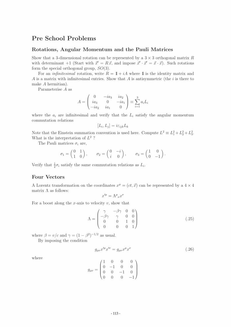
Pre School Problems
Rotations, Angular Momentum and the Pauli Matrices
Show that a 3-dimensional rotation can be represented by a 3 × 3 orthogonal matrix Rwith determinant +1 (Start with �x′ = R�x, and impose �x′ · �x′ = �x · �x). Such rotationsform the special orthogonal group, SO(3).
For an infinitesimal rotation, write R = 1l + iA where 1l is the identity matrix andA is a matrix with infinitesimal entries. Show that A is antisymmetric (the i is there tomake A hermitian).
Parameterise A as
A =
⎛⎜⎝ 0 −ia3 ia2
ia3 0 −ia1
−ia2 ia1 0
⎞⎟⎠ ≡3∑
i=1
aiLi
where the ai are infinitesimal and verify that the Li satisfy the angular momentumcommutation relations
[Li, Lj] = iεijkLk
Note that the Einstein summation convention is used here. Compute L2 ≡ L21 +L2
2 +L23.
What is the interpretation of L2 ?The Pauli matrices σi are,
σ1 =(
0 11 0
), σ2 =
(0 −ii 0
), σ3 =
(1 00 −1
).
Verify that 12σi satisfy the same commutation relations as Li.
Four Vectors
A Lorentz transformation on the coordinates xμ = (ct, �x) can be represented by a 4 × 4matrix Λ as follows:
x′μ = Λμνx
ν
For a boost along the x-axis to velocity v, show that
Λ =
⎛⎜⎜⎜⎝γ −βγ 0 0
−βγ γ 0 00 0 1 00 0 0 1
⎞⎟⎟⎟⎠ (.25)
where β = v/c and γ = (1 − β2)−1/2 as usual.By imposing the condition
gμνx′μx′ν = gμνx
μxν (.26)
where
gμν =
⎛⎜⎜⎜⎝1 0 0 00 −1 0 00 0 −1 00 0 0 −1
⎞⎟⎟⎟⎠
- 113 -

show thatgμνΛ
μρΛ
νσ = gρσ or ΛTgΛ = g
This is the analogue of the orthogonality relation for rotations. Check that it works forthe Λ given by equation (.25) above.
Now introducexμ = gμνx
ν
and show, by reconsidering equation (.26) using xμxμ, or otherwise, that
x′μ = xν(Λ
−1)νμ
Vectors Aμ and Bμ that transform like xμ and xμ are sometimes called contravariantand covariant respectively. A simpler pair of names is vector and covector. A particularlyimportant covector is obtained by letting ∂/∂xμ act on a scalar φ:
∂φ
∂xμ≡ ∂μφ
Show that ∂μ does transform like xμ and not xμ.
Probability Density and Current Density
Starting from the Schrodinger equation for the wave function ψ(�x, t), show that theprobability density ρ = ψ∗ψ satisfies the continuity equation
∂ρ
∂t+ ∇ �J = 0
where�J =
h
2im[ψ∗(∇ψ) − (∇ψ∗)ψ]
What is the interpretation of �J? Verify that the continuity equation can be written inmanifestly covariant form.
∂μJμ = 0
where Jμ = (cρ, �J).
- 114 -


![Isospin breaking studies from Lattice QCD+QED · Isospin breaking studies from Lattice QCD+QED Taku Izubuchi, [RBC-UKQCD Collaboration] Tom Blum, Takumi Doi, Masashi Hayakawa, Tomomi](https://img.dokumen.tips/doc/110x75/5e9a851aa7364020480b1633/isospin-breaking-studies-from-lattice-qcdqed-isospin-breaking-studies-from-lattice.jpg)