An Introduction to Logics of Knowledge and Belief - … · · 2015-02-20An Introduction to Logics of Knowledge and Belief Hans van Ditmarsch ... It turns out that, ... must ensure,

Chapter 1

An Introduction to Logics ofKnowledge and Belief

Hans van DitmarschJoseph Y. Halpern

Wiebe van der HoekBarteld Kooi

Contents1.1 Introduction to the Book . . . . . . . . . . . . . . 11.2 Basic Concepts and Tools . . . . . . . . . . . . . 21.3 Overview of the Book . . . . . . . . . . . . . . . . 421.4 Notes . . . . . . . . . . . . . . . . . . . . . . . . . . 45

References . . . . . . . . . . . . . . . . . . . . . . . 49

Abstract This chapter provides an introduction to some basicconcepts of epistemic logic, basic formal languages, their se-mantics, and proof systems. It also contains an overview of thehandbook, and a brief history of epistemic logic and pointers tothe literature.

1.1 Introduction to the Book

This introductory chapter has four goals:

1. an informal introduction to some basic concepts of epistemic logic;

2. basic formal languages, their semantics, and proof systems;

Chapter 1 of the Handbook of Epistemic Logic, H. van Ditmarsch, J.Y. Halpern, W. vander Hoek and B. Kooi (eds), College Publications, 2015, pp. 1–51.

2 CHAPTER 1. INTRODUCTION

3. an overview of the handbook; and

4. a brief history of epistemic logic and pointers to the literature.

In Section 1.2, we deal with the first two items. We provide examplesthat should help to connect the informal concepts with the formal defi-nitions. Although the informal meaning of the concepts that we discussmay vary from author to author in this book (and, indeed, from reader toreader), the formal definitions and notation provide a framework for thediscussion in the remainder of the book.

In Section 1.3, we outline how the basic concepts from this chapter arefurther developed in subsequent chapters, and how those chapters relate toeach other. This chapter, like all others, concludes with a section of notes,which gives all the relevant references and some historical background, anda bibliography.

1.2 Basic Concepts and Tools

As the title suggests, this book uses a formal tool, logic, to study the notionof knowledge (“episteme” in Greek, hence epistemic logic) and belief, and,in a wider sense, the notion of information.

Logic is the study of reasoning, formalising the way in which certainconclusions can be reached, given certain premises. This can be done byshowing that the conclusion can be derived using some deductive system(like the axiom systems we present in Section 1.2.5), or by arguing that thetruth of the conclusion must follow from the truth of the premises (truthis the concern of the semantical approach of Section 1.2.2). However, firstof all, the premises and conclusions need to be presented in some formallanguage, which is the topic of Section 1.2.1. Such a language allows us tospecify and verify properties of complex systems of interest.

Reasoning about knowledge and belief, which is the focus of this book,has subtleties beyond those that arise in propositional or predicate logic.Take, for instance, the law of excluded middle in classical logic, which saysthat for any proposition p, either p or ¬p (the negation of p) must hold;formally, p _ ¬p is valid. In the language of epistemic logic, we write Kapfor ‘agent a knows that p is the case’. Even this simple addition to thelanguage allows us to ask many more questions. For example, which of thefollowing formulas should be valid, and how are they related? What kindof ‘situations’ do the formulas describe?

• Kap _ ¬Kap

• Kap _ Ka¬p

1.2. BASIC CONCEPTS AND TOOLS 3

• Ka(p _ ¬p)

• Kap _ ¬Ka¬p

It turns out that, given the semantics of interest to us, only the first andthird formulas above are valid. Moreover as we will see below, Kap logicallyimplies ¬Ka¬p, so the last formula is equivalent to ¬Ka¬p, and says ‘agenta considers p possible’. This is incomparable to the second formula, whichsays agent a knows whether p is true’.

One of the appealing features of epistemic logic is that it goes beyondthe ‘factual knowledge’ that the agents have. Knowledge can be aboutknowledge, so we can write expressions like Ka(Kap ! Kaq) (a knowsthat if he knows that p, he also knows that q). More interestingly, we canmodel knowledge about other’s knowledge, which is important when wereason about communication protocols. Suppose Ann knows some fact m(‘we meet for dinner the first Sunday of August’). So we have Kam. Nowsuppose Ann e-mails this message to Bob at Monday 31st of July, and Bobreads it that evening. We then have Kbm ^ KbKam. Do we have KaKbm?Unless Ann has information that Bob has actually read the message, shecannot assume that he did, so we have (Kam ^ ¬KaKbm ^ ¬Ka¬Kbm).

We also have KaKb¬KaKbm. To see this, we already noted that ¬KaKb

m, since Bob might not have read the message yet. But if we can deducethat, then Bob can as well (we implicitly assume that all agents can doperfect reasoning), and, moreover, Ann can deduce that. Being a gentleman,Bob should resolve the situation in which ¬KaKbm holds, which he couldtry to do by replying to Ann’s message. Suppose that Bob indeed replies onTuesday morning, and Ann reads this on Tuesday evening. Then, on thatevening, we indeed have KaKbKam. But of course, Bob cannot assume Annread the acknowledgement, so we have ¬KbKaKbKam. It is obvious that ifAnn and Bob do not want any ignorance about knowledge of m, they betterpick up the phone and verify m. Using the phone is a good protocol thatguarantees Kam ^ Kbm ^ KaKbm ^ KbKam ^ KaKbKam ^ . . . , a notionthat we call common knowledge; see Section 1.2.2.

The point here is that our formal language helps clarify the effect of a(communication) protocol on the information of the participating agents.This is the focus of Chapter 12. It is important to note that requirements ofprotocols can involve both knowledge and ignorance: in the above examplefor instance, where Charlie is a roommate of Bob, a goal (of Bob) for theprotocol might be that he knows that Charlie does not know the message(Kb¬Kcm), while a goal of Charlie might even be KcKb¬m. Actually, inthe latter case, it may be more reasonable to write KcBb¬m: Charlie knowsthat Bob believes that there is no dinner on Sunday. A temporal progressionfrom Kbm ^ ¬KaKbm to KbKam can be viewed as learning. This raises


interesting questions in the study of epistemic protocols: given an initial andfinal specification of information, can we find a sequence of messages thattake us from the former to the latter? Are there optimal such sequences?These questions are addressed in Chapter 5, specifically Sections 5.7 and5.9.

Here is an example of a scenario where the question is to derive a se-quence of messages from an initial and final specification of information. Itis taken from Chapter 12, and it demonstrates that security protocols thataim to ensure that certain agents stay ignorant cannot (and do not) alwaysrely on the fact that some messages are kept secret or hidden.

Alice and Betty each draw three cards from a pack of sevencards, and Eve (the eavesdropper) gets the remaining card. Canplayers Alice and Betty learn each other’s cards without reveal-ing that information to Eve? The restriction is that Alice andBetty can make only public announcements that Eve can hear.

We assume that (it is common knowledge that) initially, all three agentsknow the composition of the pack of cards, and each agent knows whichcards she holds. At the end of the protocol, we want Alice and Betty toknow which cards each of them holds, while Eve should know only whichcards she (Eve) holds. Moreover, messages can only be public announce-ments (these are formally described in Chapter 6), which in this setting justmeans that Alice and Betty can talk to each other, but it is common know-ledge that Eve hears them. Perhaps surprisingly, such a protocol exists,and, hopefully less surprisingly by now, epistemic logic allows us to for-mulate precise epistemic conditions, and the kind of announcements thatshould be allowed. For instance, no agent is allowed to lie, and agents canannounce only what they know. Dropping the second condition would al-low Alice to immediately announce Eve’s card, for instance. Note there isan important distinction here: although Alice knows that there is an an-nouncement that she can make that would bring about the desired stateof knowledge (namely, announcing Eve’s card), there is not something thatAlice knows that she can announce that would bring about the desired stateof knowledge (since does not in fact know Eve’s card). This distinction hasbe called the de dicto/de re distinction in the literature. The connectionsbetween knowledge and strategic ability are the topic of Chapter 11.

Epistemic reasoning is also important in distributed computing. Asargued in Chapter 5, processes or programs in a distributed environmentoften have only a limited view of the global system initially; they graduallycome to know more about the system. Ensuring that each process hasthe appropriate knowledge needed in order to act is the main issue here.


The chapter mentions a number of problems in distributed systems whereepistemic tools are helpful, like agreement problems (the dinner example ofAnn and Bob above would be a simple example) and the problem of mutualexclusion, where processes sharing a resource must ensure that only oneprocess uses the resource at a time. An instance of the latter is provided inChapter 8, where epistemic logic is used to specify a correctness property ofthe Railroad Crossing System. Here, the agents Train, Gate and Controllermust ensure, based on the type of signals that they send, that the train isnever at the crossing while the gate is ‘up’. Chapter 8 is on model checking;it provides techniques to automatically verify that such properties (specifiedin an epistemic temporal language; cf. Chapter 5) hold. Epistemic tools todeal with the problem of mutual exclusion are also discussed in Chapter 11,in the context of dealing with shared file updates.

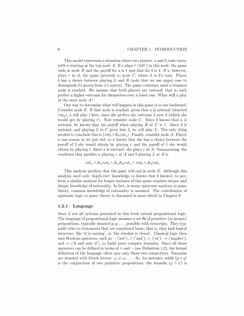
Reasoning about knowing what others know (about your knowledge)is also typical in strategic situations, where one needs to make a decisionbased on how others will act (where the others, in turn, are basing theirdecision on their reasoning about you). This kind of scenario is the focusof game theory. Epistemic game theory studies game theory using notionsfrom epistemic logic. (Epistemic game theory is the subject of Chapter 9in this book.) Here, we give a simplified example of one of the main ideas.Consider the game in Figure 1.1.

✓

14

◆

✓

22

◆

✓

41

◆

A

B C

D E

F G

l

l r

r

L R

a

b

a

✓

33

◆

Figure 1.1: A simple extensive form game.


This model represents a situation where two players, a and b, take turns,with a starting at the top node A. If a plays l (‘left’) in this node, the gameends in node B and the payoff for a is 1 and that for b is 4. If a, however,plays r in A, the game proceeds to node C, where it is b’s turn. Playerb has a choice between playing L and R (note that we use upper case todistinguish b’s moves from a’s moves). The game continues until a terminalnode is reached. We assume that both players are rational; that is, eachprefers a higher outcome for themselves over a lower one. What will a playin the start node A?

One way to determine what will happen in this game is to use backward.Consider node E. If that node is reached, given that a is rational (denotedrata), a will play l here, since she prefers the outcome 4 over 3 (which shewould get by playing r). Now consider node C. Since b knows that a isrational, he knows that his payoff when playing R at C is 1. Since b isrational, and playing L in C gives him 2, he will play L. The only thingneeded to conclude this is (ratb^Kbrata). Finally, consider node A. Playera can reason as we just did, so a knows that she has a choice between thepayoff of 2 she would obtain by playing r and the payoff of 1 she wouldobtain by playing l. Since a is rational, she plays r at A. Summarising, thecondition that justifies a playing r at A and b playing L at B is

rata ^ Karatb ^ KaKbrata ^ ratb ^ Kbrata

This analysis predicts that the game will end in node D. Although thisanalysis used only ‘depth-two’ knowledge (a knows that b knows), to per-form a similar analysis for longer variants of this game requires deeper anddeeper knowledge of rationality. In fact, in many epistemic analyses in gametheory, common knowledge of rationality is assumed. The contribution ofepistemic logic to game theory is discussed in more detail in Chapter 9.

1.2.1 Language

Most if not all systems presented in this book extend propositional logic.The language of propositional logic assumes a set At of primitive (or atomic)propositions, typically denoted p, q, . . . , possibly with subscripts. They typ-ically refer to statements that are considered basic; that is, they lack logicalstructure, like ‘it is raining’, or ‘the window is closed’. Classical logic thenuses Boolean operators, such as ¬ (‘not’), ^ (‘and’), _, (‘or’), ! (‘implies’),and $ (‘if and only if’), to build more complex formulas. Since all thoseoperators can be defined in terms of ^ and ¬ (see Definition 1.2), the formaldefinition of the language often uses only these two connectives. Formulasare denoted with Greek letters: ', ,↵, . . . . So, for instance, while (p ^ q)is the conjunction of two primitive propositions, the formula (' ^ ) is


a conjunction of two arbitrary formulas, each of which may have furtherstructure.

When reasoning about knowledge and belief, we need to be able torefer to the subject, that is, the agent whose knowledge or belief we aretalking about. To do this, we assume a finite set Ag of agents. Agents aretypically denoted a, b, . . . , i, j, . . . , or, in specific examples, Alice,Bob, . . . .To reason about knowledge, we add operators Ka to the language of classicallogic, where Ka' denotes ‘agent a knows (or believes) '’. We typically letthe context determine whether Ka represents knowledge or belief. If it isnecessary to reason knowledge and belief simultaneously, we use operatorsKa for knowledge and Ba for belief. Logics for reasoning about knowledgeare sometimes called epistemic logics, while logics for reasoning about beliefare called doxastic logics, from the Greek words for knowledge and belief.The operators Ka and Ba are examples of modal operators. We sometimesuse 2 or 2a to denote a generic modal operator, when we want to discussgeneral properties of modal operators.

Definition 1.1 (An Assemblage of Modal Languages)Let At be a set of primitive propositions, Op a set of modal operators, andAg a set of agent symbols. Then we define the language L(At,Op,Ag) bythe following BNF:

' := p | ¬' | (' ^ ') | 2',

where p 2 At and 2 2 Op. a

Typically, the set Op depends on Ag. For instance, the language formulti-agent epistemic logic is L(At,Op,Ag), with Op = {Ka | a 2 Ag}, thatis, we have a knowledge operator for every agent. To study interactionsbetween knowledge and belief, we would have Op = {Ka, Ba | a 2 Ag}. Thelanguage of propositional logic, which does not involve modal operators, isdenoted L(At); propositional formulas are, by definition, formulas in L(At).

Definition 1.2 (Abbreviations in the Language)As usual, parentheses are omitted if that does not lead to ambiguity. Thefollowing abbreviations are also standard (in the last one, A ✓ Ag).

description/name definiendum definiensfalse ? p ^ ¬ptrue > ¬?disjunction ' _ ¬(¬' ^ ¬ )implication ' ! ¬' _ dual of K Ma' or K̂a' ¬Ka¬'everyone in A knows EA'

V

a2A Ka'


Note that Ma', which say ‘agent a does not know ¬'’, can also be read‘agent a considers ' possible’. a

Let 2 be a modal operator, either one in Op or one defined as an ab-breviation. We define the nth iterated application of 2, written 2n, asfollows:

20' = ' and 2n+1' = 22n'.

We are typically interested in iterating the EA operator, so that we cantalk about ‘everyone in A knows’, ‘everyone in A knows that everyone in Aknows’, and so on.

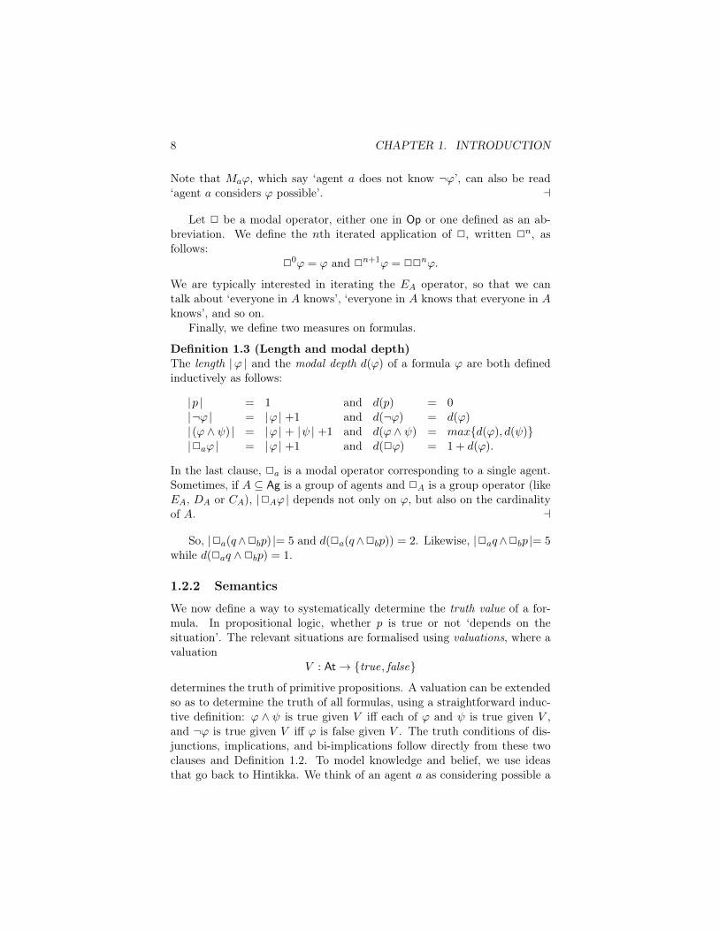
Finally, we define two measures on formulas.

Definition 1.3 (Length and modal depth)The length |' | and the modal depth d(') of a formula ' are both definedinductively as follows:

|p | = 1 and d(p) = 0|¬' | = |' | +1 and d(¬') = d(')|(' ^ ) | = |' | + | | +1 and d(' ^ ) = max{d('), d( )}|2a' | = |' | +1 and d(2') = 1 + d(').

In the last clause, 2a is a modal operator corresponding to a single agent.Sometimes, if A ✓ Ag is a group of agents and 2A is a group operator (likeEA, DA or CA), |2A' | depends not only on ', but also on the cardinalityof A. a

So, |2a(q ^2bp) |= 5 and d(2a(q ^2bp)) = 2. Likewise, |2aq ^2bp |= 5while d(2aq ^ 2bp) = 1.

1.2.2 Semantics

We now define a way to systematically determine the truth value of a for-mula. In propositional logic, whether p is true or not ‘depends on thesituation’. The relevant situations are formalised using valuations, where avaluation

V : At ! {true, false}determines the truth of primitive propositions. A valuation can be extendedso as to determine the truth of all formulas, using a straightforward induc-tive definition: ' ^ is true given V iff each of ' and is true given V ,and ¬' is true given V iff ' is false given V . The truth conditions of dis-junctions, implications, and bi-implications follow directly from these twoclauses and Definition 1.2. To model knowledge and belief, we use ideasthat go back to Hintikka. We think of an agent a as considering possible a


number of different situations that are consistent with the information thatthe agent has. Agent a is said to know (or believe) ', if ' is true in allthe situations that a considers possible. Thus, rather than using a singlesituation to give meaning to modal formulas, we use a set of such situations;moreover, in each situation, we consider, for each agent, what other situa-tions he or she considers possible. The following example demonstrates howthis is done.

Example 1.1Bob is invited for a job interview with Alice. They have agreed that itwill take place in a coffeehouse downtown at noon, but the traffic is quiteunpredictable, so it is not guaranteed that either Alice or Bob will arriveon time. However, the coffeehouse is only a 15-minute walk from the busstop where Alice plans to go, and a 10-minute walk from the metro stationwhere Bob plans to go. So, 10 minutes before the interview, both Alice andBob will know whether they themselves will arrive on time. Alice and Bobhave never met before. A Kripke model describing this situation is given inFigure 1.2.

u

vta, tb ta, ¬tb

s

w

¬ta, tb ¬ta, ¬tb

a

a

bb

a, b a, b

a, b a, b

Figure 1.2: The Kripke model for Example 1.1.

Suppose that at 11:50, both Alice and Bob have just arrived at theirrespective stations. Taking ta and tb to represent that Alice (resp., Bob)arrive on time, this is a situation (denoted w in Figure 1.2) where both taand tb are true. Alice knows that ta is true (so in w we have Kata), but shedoes not know whether tb is true; in particular, Alice considers possible thesituation denoted v in Figure 1.2, where ta ^¬tb holds. Similarly, in w, Bobconsiders it possible that the actual situation is s, where Alice is runninglate but Bob will make it on time, so that ¬ta ^ tb holds. Of course, in s,Alice knows that she is late; that is, Ka¬ta holds. Since the only situations


that Bob considers possible at world w are w and s, he knows that he willbe on time (Kbtb), and knows that Alice knows whether or not she is ontime (Kb(Kata_Ka¬ta)). Note that the latter fact follows since Kata holdsin world w and Ka¬ta holds in world s, so Kata _ Ka¬ta holds in bothworlds that Bob considers possible. a

This, in a nutshell, explains what the models for epistemic and doxasticlook like: they contain a number of situations, typically called states or(possible) worlds, and binary relations on states for each agent, typicallycalled accessibility relations. A pair (v, w) is in the relation for agent a if,in world v, agent a considers state w possible. Finally, in every state, weneed to specify which primitive propositions are true.

Definition 1.4 (Kripke frame, Kripke model)Given a set At of primitive propositions and a set Ag of agents, a Kripkemodel is a structure M = hS, RAg, V At), where

• S 6= ; is a set of states, sometimes called the domain of M , anddenoted D(M);

• RAg is a function, yielding an accessibility relation Ra ✓ S ⇥ S foreach agent a 2 Ag;

• V At : S ! (At ! {true, false}) is a function that, for all p 2 At ands 2 S, determines what the truth value V At(s)(p) of p is in state s (soV At(s) is a propositional valuation for each s 2 S).

We often suppress explicit reference to the sets At and Ag, and write M =hS, R, V i, without upper indices. Further, we sometimes write sRat orRast rather than (s, t) 2 Ra, and use Ra(s) or Ras to denote the set {t 2S | Rast}. Finally, we sometimes abuse terminology and refer to V as avaluation as well.

The class of all Kripke models is denoted K. We use Km to denote theclass of Kripke models where |Ag |= m. A Kripke frame F = hS, Ri focuseson the graph underlying a model, without regard for the valuation. a

More generally, given a modal logic with a set Op of modal operators,the corresponding Kripke model has the form M = hS, ROp, V Ati, wherethere is a binary relation R2 for every operator 2 2 Op. Op may, forexample, consist of a knowledge operator for each agent in some set Ag anda belief operator for each agent in Ag.

Given Example 1.1 and Definition 1.4, it should now be clear how thetruth of a formula is determined given a model M and a state s. A pair(M, s) is called a pointed model; we sometimes drop the parentheses andwrite M, s.


Definition 1.5 (Truth in a Kripke Model)Given a model M = hS, RAg, V Ati, we define what it means for a formula 'to be true in (M, s), written M, s |= ', inductively as follows:

M, s |= p iff V (s)(p) = true for p 2 AtM, s |= ' ^ iff M, s |= ' and M, s |= M, s |= ¬' iff not M, s |= ' (often written M, s 6|= ')M, s |= Ka' iff M, t |= ' for all t such that Rast.

More generally, if M = hS, ROp, V Ati, then for all 2 2 Op:

M, s |= 2' iff (M, t) |= ' for all t such that R2st.

Recall that Ma is the dual of Ka; it easily follows from the definitions that

M, s |= Ma' iff there exists some t such that Rast and M, t |= '.

We write M |= ' if M, s |= ' for all s 2 S. a

Example 1.2Consider the model of Figure 1.2. Note that Kap_Ka¬p represents the factthat agent a knows whether p is true. Likewise, Map ^ Ma¬p is equivalentto ¬Ka¬p ^ ¬Kap: agent a is ignorant about p. We have the following (inthe final items we write Eab instead of E{a,b}):

1. (M, s) |= tb: truth of a primitive proposition in s.

2. M, s |= (¬ta ^ Ka¬ta ^ ¬Kb¬ta) ^ (tb ^ ¬Katb ^ Kbtb): at s, a knowsthat ta is false, but b does not; similarly, b knows that tb is true, buta does not.

3. M |= Ka(Kbtb _Kb¬tb)^Kb(Kata _Ka¬ta): in all states of M , agenta knows that b knows whether tb is true, and b knows that a knowswhether ta is true.

4. M |= Ka(Mbtb^Mb¬tb)^Kb(Mata^Ma¬ta) in all states of M , agenta knows that b does not know whether ta is true, and b knows that adoes not know whether tb is true.

5. M |= Eab((Kata _ Ka¬ta) ^ (Matb ^ Ma¬tb)): in all states, everyoneknows that a knows whether ta is true, but a does not know whethertb is true.

6. M |= EabEab((Kata_Ka¬ta)^(Matb^Ma¬tb)): in all states, everyoneknows what we stated in the previous item.


This shows that the model M of Figure 1.2 is not just a model for a situationwhere a knows ta but not tb and agent b knows tb but not ta; it representsmuch more information. a

As the following example shows, in order to model certain situations,it may be necessary that some propositional valuations occur in more thanone state in the model.Example 1.3Recall the scenario of the interview between Alice and Bob, as presented inExample 1.1. Suppose that we now add the information that in fact Alicewill arrive on time, but Bob is not going to be on time. Although Bob doesnot know Alice, he knows that his friend Carol is an old friend of Alice.Bob calls Carol, leaving a message on her machine to ask her to informAlice about Bob’s late arrival as soon as she is able to do so. Unfortunatelyfor Bob, Carol does not get his message on time. This situation can berepresented in state M, v of the model of Figure 1.3.

u

vta, tb ta, ¬tb

s

w

¬ta, tb ¬ta, ¬tb

a

a

bb

a, b a, b

a, b a, b

a, b

¬ta, ¬tb

a, b

v0

u0

ta, ¬tb

b

b

b

b b

Figure 1.3: The Kripke model for Example 1.3.

Note that in (M, v), we have ¬Ka¬tb (Alice does not know that Bobis late), but also Mb(Ka¬tb) (Bob considers it possible that Alice knowsthat Bob is late). So, although the propositional valuations in v and v0 arethe same, those two states represent different situations: in v agent a isuncertain whether ¬tb holds, while in v0 she knows ¬tb. Also, in M, v, Bobconsiders it possible that both of them will be late, and that Alice knowsthis: this is because Rbvu0 holds in the model, and M, u0 |= Ka(¬ta^¬tb).a

We often impose restrictions on the accessibility relation. For example,we may want to require that if, in world v, agent a considers world w possi-


ble, then in w, agent a should consider v possible. This requirement wouldmake Ra symmetric. Similarly, we might require that, in each world w, aconsiders w itself possible. This would make Ra reflexive. More generally,we are interested in certain subclasses of models (typically characterized byproperties of the accessibility relations).

Definition 1.6 (Classes of models, validity, satisfiability)Let X be a class of models, that is, X ✓ K. If M |= ' for all models M inX , we say that ' is valid in X , and write X |= '. For example, for validityin the class of all Kripke models K, we write K |= '. We write X 6|= ' whenit is not the case that X |= '. So X 6|= ' holds if, for some model M 2 Xand some s 2 D(M), we have M, s |= ¬'. If there exists a model M 2 Xand a state s 2 D(M) such that M, s |= ', we say that ' is satisfiable inX . a

We now define a number of classes of models in terms of properties of therelations Ra in those models. Since they depend only on the accessibilityrelation, we could have defined them for the underlying frames; indeed, theproperties are sometimes called frame properties.

Definition 1.7 (Frame properties)Let R be an accessibility relation on a domain of states S.

1. R is serial if for all s there is a t such that Rst. The class of se-rial Kripke models, that is, {M = hS, R, V i | every Ra is serial} isdenoted KD.

2. R is reflexive if for all s, Rss. The class of reflexive Kripke models isdenoted KT .

3. R is transitive if for all s, t, u, if Rst and Rtu then Rsu. The class oftransitive Kripke models is denoted K4.

4. R is Euclidean if for all s, t, and u, if Rst and Rsu then Rtu. Theclass of Euclidean Kripke models is denoted K5

5. R is symmetric if for all s, t, if Rst then Rts. The class of symmetricKripke models is denoted KB

6. We can combine properties of relations:

(a) The class of reflexive transitive models is denoted S4.

(b) The class of transitive Euclidean models is denoted K45.

(c) The class of serial transitive Euclidean models is denoted KD45.


(d) R is an equivalence relation if R is reflexive, symmetric, andtransitive. It not hard to show that R is an equivalence relationif R is reflexive and Euclidean. The class of models where therelations are equivalence relations is denoted S5.

As we did for Km, we sometimes use the subscript m to denote the numberof agents, so S5m, for instance, is the class of Kripke models with |Ag |= m.a

Of special interest in this book is the class S5. In this case, the accessi-bility relations are equivalence classes. This makes sense if we think of Rastholding if s and t are indistinguishable by agent a based on the informationthat a has received. S5 has typically been used to model knowledge. In anS5 model, write s ⇠a t rather than Rast, to emphasize the fact that Ra isan equivalence relation. When it is clear that M 2 S5, when drawing themodel, we omit reflexive arrows, and since the relations are symmetric, weconnect states by a line, rather than using two-way arrows. Finally, we leaveout lines that can be deduced to exist using transitivity. We call this the S5representation of a Kripke model. Figure 1.4 shows the S5 representationof the Kripke model of Figure 1.3.

u

vta, tb ta, ¬tb

s

w

¬ta, tb ¬ta, ¬tb

a

a

bb

¬ta, ¬tb

v0

u0

ta, ¬tb

b

b

b

Figure 1.4: The S5 representation of the Kripke model in Figure 1.3.

When we restrict the classes of models considered, we get some inter-esting additional valid formulas.

Theorem 1.1 (Valid Formulas)Parts (c)–(i) below are valid formulas, where ↵ is a substitution instance ofa propositional tautology (see below), ' and are arbitrary formulas, andX is one of the classes of models defined in Definition 1.7; parts (a), (b),and (j) show that we can infer some valid formulas from others.

(a) If X |= ' ! and X |= ', then X |= .

(b) If X |= ' then X |= K'.

(c) X |= ↵.


(d) X |= K(' ! ) ! (K' ! ).

(e) KD |= K' ! M'.

(f) T |= K' ! '.

(g) K4 |= K' ! KK'.

(h) K5 |= ¬K' ! K¬K'.

(i) KB |= ' ! KM'.

(j) If X ✓ Y then Y |= ' implies that X |= '. a

Since S5 is the smallest of the classes of models considered in Definition 1.7,it easily follows that all the formulas and inference rules above are valid inS5. To the extent that we view S5 as the class of models appropriatefor reasoning about knowledge, Theorem 1.1 can be viewed as describingproperties of knowledge. As we shall see, many of these properties apply tothe standard interpretation of belief as well.

Parts (a) and (c) emphasise that we represent knowledge in a logicalframework: modus ponens is valid as a reasoning rule, and we take allpropositional tautologies for granted. In part (c), ↵ is a substitution instanceof a propositional tautology. For example, since p _ ¬p and p ! (q ! p)are propositional tautologies, ↵ could be Kp _ ¬Kp or K(p _ q) ! (Kr !K(p _ q)). That is, we can substitute an arbitrary formula (uniformly)for a primitive proposition in a propositional tautology. Part (b) says thatagents know all valid formulas, and part (d) says that an agent is ableto apply modus ponens to his own knowledge. Part (e) is equivalent toK' ! ¬K¬'; an agent cannot at the same time know a proposition andits negation. Part (f) is even stronger: it says that what an agent knowsmust be true. Parts (g) and (h) represent what has been called positive andnegative introspection, respectively: an agent knows what he knows andwhat he does not know. Part (i) can be shown to follow from the othervalid formulas; it says that if something is true, the agent knows that heconsiders it possible.

Notions of Group Knowledge

So far, all properties that we have encountered are properties of an indi-vidual agent’s knowledge. such as EA, defined above. In this section weintroduce two other notions of group knowledge, common knowledge CA

and distributed knowledge DA, and investigate their properties.


Example 1.4 (Everyone knows and distributed knowledge)Alice and Betty each has a daughter; their children can each either be atthe playground (denoted pa and pb, respectively) or at the library (¬pa,and ¬pb, respectively). Each child has been carefully instructed that, if sheends up being on the playground without the other child, she should callher mother to inform her. Consider the situation described by the modelM in Figure 1.5.

s

w

t

u

a a

b b

a, b

¬pa, pb

¬pa, ¬pb

pa, ¬pb

pa, pb

Figure 1.5: The (S5 representation of the) model for Example 1.4.

We have

M |= ((¬pa ^ pb) $ Ka(¬pa ^ pb)) ^ ((pa ^ ¬pb) $ Kb(pa ^ ¬pb)).

This models the agreement each mother made with her daughter. Nowconsider the situation at state s. We have M, s |= Ka¬(pa ^ ¬pb), thatis, Alice knows that it is not the case that her daughter is alone at theplayground (otherwise her daughter would have informed her). What doeseach agent know at s? If we consider only propositional facts, it is easyto see that Alice knows pa ! pb and Betty knows pb ! pa. What doeseveryone know at s? The following sequence of equivalences is immediatefrom the definitions:

M, s |= E{a,b}'iff M, s |= Ka' ^ Kb'iff 8x(Rasx ) M, x |= ') and 8y(Rbsy ) M, y |= ')iff 8x 2 {s, w, t} (M, x |= ') and 8y 2 {s, u, t} (M, y |= ')iff M |= '.

Thus, in this model, what is known by everyone are just the formulas validin the model. Of course, this is not true in general.

Now suppose that Alice and Betty an opportunity to talk to each other.Would they gain any new knowledge? They would indeed. Since M, s |=


Ka(pa ! pb) ^ Kb(pb ! pa), they would come to know that pa $ pb holds;that is, they would learn that their children are at least together, whichis certainly not valid in the model. The knowledge that would emerge ifthe agents in a group A were allowed to communicate is called distributedknowledge in A, and denoted by the operator DA. In our example, we haveM, s |= D{a,b}(pa $ pb), although M, s |= ¬Ka(pa $ pb) ^ ¬Kb(pa $ pb).In other words, distributed knowledge is generally stronger than any indi-vidual’s knowledge, and we therefore cannot define DA' as

W

i2A Ki', thedual of general knowledge that we may have expected; that would be weakerthan any individual agent’s knowledge. In terms of the model, what wouldhappen if Alice and Betty could communicate is that Alice could tell Bettythat he should not consider state u possible, while Betty could tell Alicethat she should not consider state w possible. So, after communication, theonly states considered possible by both agents at state s are s and t. Thisargument suggests that we should interpret DA as the necessity operator(2-type modal operator) of the relation

T

a2A Ra. By way of contrast, it fol-lows easily from the definitions that EA can be interpreted as the necessityoperator of the relation

S

a2A Ra. aThe following example illustrates common knowledge.

Example 1.5 (Common knowledge)This time we have two agents: a sender (s) and a receiver (r). If a messageis sent, it is delivered either immediately or with a one-second delay. Thesender sends a message at time t0. The receiver does not know that thesender was planning to send the message. What is each agent’s state ofknowledge regarding the message?

To reason about this, let sz (for z 2 Z) denote that the message was sentat time t0+z, and, likewise, let dz denote that the message was delivered attime t = z. Note that we allow z to be negative. To see why, consider theworld w0,0 where the message arrives immediately (at time t0). (In general,in the subscript (i, j) of a world wi,j , i denotes the time that the messagewas sent, and j denotes the time it was received.) In world w0,0, the receiverconsiders it possible that the message was sent at time t0 � 1. That is, thereceiver considers possible the world w�1,0 where the message was sent att0 � 1 and took one second to arrive. In world w�1,0, the sender considerspossible the world w�1,�1 where the message was sent at time t0 � 1 andarrived immediately. And in world w�1,�1, the receiver considers possiblea world w�2,�1 where the message as sent at time t0 � 2. (In general, inworld wn,m, the message is sent at time t0 +n and received at time t0 +m.)In addition, in world w0,0, the sender considers possible world w0,1, wherethe message is received at time t0 + 1. The situation is described in thefollowing model M .


(s0, d0) (s�1, d0) (s�1, d�1) (s�2, d�1) (s�2, d�2)

(s0, d1) (s1, d1) (s1, d2) (s2, d2) (s2, d3)

s

s

s

s

s

r

r r

r

Figure 1.6: The (S5 representation of the) model for Example 1.5.

Writing E for ‘the sender and receiver both know’, it easily follows that

M, w0,0 |= s0 ^ d0 ^ ¬E¬s�1 ^ ¬E¬d1 ^ ¬E3¬s�2.

The notion of ' being common knowledge among group A, denoted CA',is meant to capture the idea that, for all n, En' is true. Thus, ' is notcommon among A if someone in A considers it possible that someone in Aconsiders it possible that . . . someone in A considers it possible that ' isfalse. This is formalised below, but the reader should already be convincedthat in our scenario, even if it is common knowledge among the agents thatmessages will have either no delay or a one-second delay, it is not commonknowledge that the message was sent at or after time t0 � m for any valueof m! aDefinition 1.8 (Semantics of three notions of group knowledge)Let A ✓ Ag be a group of agents. Let REA

= [a2ARa. As we observedabove,

(M, s) |= EA' iff for all t such that REAst, we have (M, t) |= '.

Similarly, taking RDA= \a2ARa, we have

(M, s) |= DA' iff for all t such that RDAst, we have (M, t) |= '.

Finally, recall that the transitive closure of a relation R is the smallestrelation R+ such that R ✓ R+, and such that, for all x, y, and z, if R+xyand R+yz then R+xz. We define RCA

as R+EA

= (S

a2A Ra)+. Note that,in Figure 1.6, every pair of states is in the relation R+

C{r,s}. In general, we

have RCAst iff there is some path s = s0, s1, . . . , sn = t from s to t such

that n � 1 and, for all i < n, there is some agent a 2 A for which Rasisi+1.Define

(M, s) |= CA' iff for all t such that RCAst, (M, t) |= '.

It is almost immediate from the definitions that, for a 2 A, we have

K |= (CA' ! EA') ^ (EA' ! Ka') ^ (Ka' ! DA'). (1.1)


Moreover, for T (and hence also for S4 and S5), we have

T |= Da' ! '.

The relative strengths shown in (1.1) are strict in the sense that noneof the converse implications are valid (assuming that A 6= {a}).

We conclude this section by defining some languages that are usedlater in this chapter. Fixing At and Ag, we write LX for the languageL(At,Op,Ag), where

X = K if Op = {Ka | a 2 Ag}X = CK if Op = {Ka, CA | a 2 Ag, A ✓ Ag}X = DK if Op = {Ka, DA | a 2 Ag, A ✓ Ag}X = CDK if Op = {Ka, CA, DA | a 2 Ag, A ✓ Ag}X = EK if Op = {Ka, EA | a 2 Ag, A ✓ Ag}.

Bisimulation

It may well be that two models (M, s) and (M 0, s0) ‘appear different’, butstill satisfy the same formulas. For example, consider the models (M, s),(M 0, s0), and (N, s1) in Figure 1.7. As we now show, they satisfy the sameformulas. We actually prove something even stronger. We show that allof (M, s), (M, t), (M 0, s0), (N, s1), (M, s2), and (N, s3) satisfy the sameformulas, as do all of (M, u), (M, w), (M 0, w0), (N, w1), and (N, w2). Forthe purposes of the proof, call the models in the first group green, andthe models in the second group red. We now show, by induction on thestructure of formulas, that all green models satisfy the same formulas, asdo all red models. For primitive propositions, this is immediate. And if twomodels of the same colour agree on two formulas, they also agree on theirnegations and their conjunctions. The other formulas we need to considerare knowledge formulas. Informally, the argument is this. Every agentconsiders, in every pointed model, both green and red models possible. Sohis knowledge in each pointed model is the same. We now formalise thisreasoning.

Definition 1.9 (Bisimulation)Given models M = (S, R, V ) and M 0 = (S0, R0, V 0), a non-empty relationR ✓ S ⇥S0 is a bisimulation between M and M 0 iff for all s 2 S and s0 2 S0

with (s, s0) 2 R:

• V (s)(p) = V 0(s0)(p) for all p 2 At;

• for all a 2 Ag and all t 2 S, if Rast, then there is a t0 2 S0 such thatR0

as0t0 and (t, t0) 2 R;


• for all a 2 Ag and all t0 2 S0, if R0as

0t0, then there is a t 2 S such thatRast and (t, t0) 2 R.

We write (M, s)$(M 0, s0) iff there is a bisimulation between M and M 0

linking s and s0. If so, we call (M, s) and (M 0, s0) bisimilar. a

Figure 1.7 illustrates some bisimilar models. In terms of the models

s

w

t

up, ¬q

p, q

p, ¬q

p, q

MM 0 p, ¬q

p, qs0

w0

a, b

s1 w1 w2s2 s3

p, q p, q p, qp, ¬q p, ¬q

a, b a, b a, b a, b

N

a, b a, b

a, ba, b

Figure 1.7: Bisimilar models.

of Figure 1.7, we have M, s$M 0, s0, M, s$N, s1, etc. We are interestedin bisimilarity because, as the following theorem shows, bisimilar modelssatisfy the same formulas involving the operators Ka and CA.

Theorem 1.2 (Preservation under bisimulation)Suppose that (M, s)$(M 0, s0). Then, for all formulas ' 2 LCK , we have

M, s |= ' , M 0, s0 |= '. a

The proof of the theorem proceeds by induction on the structure of formulas,much as in our example. We leave the details to the reader.

Note that Theorem 1.2 does not claim that distributed knowledge is pre-served under bisimulation, and indeed, it is not, i.e., Theorem 1.2 does nothold for a language with DA as an operator. Figure 1.8 provides a witness forthis. We leave it to the reader to check that although (M, s)$(N, s1) for thetwo pointed models of Figure 1.8, we nevertheless have (M, s) |= ¬D{a,b}pand (N, s1) |= D{a,b}p.

We can, however, generalise the notion of bisimulation to that of a groupbisimulation and ‘recover’ the preservation theorem, as follows. If A ✓ Ag,


s ta, b

pa

b

p p

a

b

¬p

¬p

M N

¬p

s1 s2

t2

t1

Figure 1.8: Two bisimilar models that do not preserve distributed know-ledge.

s and t are states, then we write RAst if A = {a | Rast}. That is, RAstholds if the set of agents a for which s and t are a-connected is exactly A.(M, s) and (M 0, s0) are group bisimilar, written (M, s)$group(M 0, s0), if theconditions of Definition 1.9 are met when every occurrence of an individualagent a is replaced by the group A. Obviously, being group bisimilar impliesbeing bisimilar. Note that the models (M, s) and (N, s1) of Figure 1.8 arebisimilar, but not group bisimilar. The proof of Theorem 1.3 is analogousto that of Theorem 1.2.

Theorem 1.3 (Preservation under bisimulation)Suppose that (M, s)$group(M 0, s0). Then, for all formulas ' 2 LCDK , wehave

M, s |= ' , M 0, s0 |= '. a

1.2.3 Expressivity and Succinctness

If a number of formal languages can be used to model similar phenomena,a natural question to ask is which language is ‘best’. Of course, the answerdepends on how ‘best’ is measured. In the next section, we compare vari-ous languages in terms of the computational complexity of some reasoningproblems. Here, we consider the notions of expressivity (what can be ex-pressed in the language?) and succinctness (how economically can one sayit?).

Expressivity

To give an example of expressivity and the tools that are used to study it, westart by showing that finiteness of models cannot be expressed in epistemiclogic, even if the language includes operators for common knowledge anddistributed knowledge.


Theorem 1.4There is no formula ' 2 LCDK such that, for all S5-models M = hS, R, V i,

M |= ' iff S is finite aProof Consider the two models M and M 0 of Figure 1.9. Obviously,

s

pM

s1 s2 s3

p p

a, b a, b a, b a, b

M 0

a, b

s4

pp

Figure 1.9: A finite and an infinite model where the same formulas are valid.

M is finite and M 0 is not. Nevertheless, the two models are easily seen tobe group bisimilar, so they cannot be distinguished by epistemic formulas.More precisely, for all formulas ' 2 LCDK , we have M, s |= ' iff M 0, s1 |= 'iff M 0, s2 |= ' iff M 0, sn |= ' for some n 2 N, and hence M |= ' iff M 0 |= '.a

It follows immediately from Theorem 1.4 that finiteness cannot be ex-pressed in the language LCDK in a class X of models containing S5.

We next prove some results that let us compare the expressivity of twodifferent languages. We first need some definitions.Definition 1.10Given a class X of models, formulas '1 and '2 are equivalent on X , written'1 ⌘X '2, if, for all (M, s) 2 X , we have that M, s |= '1 iff M, s |= '2.Language L2 is at least as expressive as L1 on X , written L1 vX L2 if, forevery formula '1 2 L1, there is a formula '2 2 L2 such that '1 ⌘X '2. L1and L2 are equally expressive on X if L1 vX L2 and L2 vX L1. If L1 vX L2but L2 6vX L1, then L2 is more expressive than L1 on X , written L1 <X L2.a

Note that if Y ✓ X , then L1 vX L2 implies L1 vY L2, while L1 6vY L2implies L1 6vX L2. Thus, the strongest results that we can show for theclasses of models of interest to us are L1 vK L2 and L1 6vS5 L2

With these definitions in hand, we can now make precise that commonknowledge ‘really adds’ something to epistemic logic.Theorem 1.5LK vK LCK and LK 6vS5 LCK . a


Proof Since LK ✓ LCK , it is obvious that LK vK LCK . To show thatLCK 6vS5 LK , consider the sets of pointed models M = {(Mn, s1) | n 2 N}and N = {(Nn, t1) | n 2 N} shown in Figure 1.10. The two models Mn andNn differ only in (Mn, sn+1) (where p is false) and (Nn, tn+1) (where p istrue). In particular, the first n � 1 states of (Mn, s1) and (Nn, t1) are thesame. As a consequence, it is easy to show that,

for all n 2 N and ' 2 LK with d(') < n, (Mn, s1) |= ' iff (Nn, t1) |= '.(1.2)

Clearly M |= C{a,b}¬p while N |= ¬C{a,b}¬p. If there were a formula' 2 LK equivalent to C{a,b}¬p, then we would have M |= ' while N |= ¬'.Let d = d('), and consider the pointed models (Md+1, s1) and (Nd+1, t1).Since the first is a member of M and the second of N , the pointed modelsdisagree on C{a,b}¬p; however, by (1.2), they agree on '. This is obviouslya contradiction, therefore a formula ' 2 L that is equivalent to C{a,b}¬pdoes not exist.

a

a

s1 s2a

as1 s2 s3

b a b

as1 s2 s3

bs4 aa b

t1

t1

t1

t2

t2

t2

t3

t3 t4

p

p

p

M1

M2

M3 N3

N2

N1

Figure 1.10: Models Mn and Nn. The atom p is only true in the pointedmodels (Nn, sn+1).

a

The next result shows, roughly speaking, that distributed knowledge isnot expressible using knowledge and common knowledge, and that commonknowledge is not expressible using knowledge and distributed knowledge.

Theorem 1.6(a) LK vK LDK and LK 6vS5 LDK ;

(b) LCK 6vS5 LDK ;

(c) LDK 6vS5 LCK ;


(d) LCK vK LCDK and LCDK 6vS5 LCK ;

(e) LDK vK LCDK and LCDK 6vS5 LDK . a

Proof For part (a), vK holds trivially. We use the models in Figure 1.8 toshow that LDK 6vS5 LK . Since (M, s)$(N, s1), the models verify the sameL-formulas. However, LDK discriminates them: we have (M, s) |= ¬D{a,b}p,while (N, s1) |= D{a,b}p. Since (M, s) and (N, s1) also verify the same LCK-formulas, part (3) also follows.

For part (b), observe that (1.2) is also true for all formulas ' 2 LDK , sothe formula C{a,b}¬p 2 LCK is not equivalent to a formula in LDK .

Part (c) is proved using exactly the same models and argument as part(a).

For part (d), v is obvious. To show that LCDK 6vS5 LDK , we can usethe models and argument of part (b). Similarly, for part (e), v is obvious.To show that LCDK 6vS5 LDK , we can use the models and argument of part(a). a

We conclude this discussion with a remark about distributed knowledge.We informally described distributed knowledge in a group as the knowledgethat would obtain were the agents in that group able to communicate.However, Figure 1.8 shows that this intuition is not quite right. First,observe that both a and b know the same formulas in (M, s) and (N, s1);they even know the same formulas in (M, s) and (N, s1). That is, for all' 2 LK , we have

(M, s) |= Ka' iff (M, s) |= Kb' iff (N, s1) |= Ka' iff (N, s1) |= Kb'

But if both agents possess the same knowledge in (N, s1), how can com-munication help them in any way, that is, how can it be that there isdistributed knowledge (of p) that no individual agent has? Similarly, if ahas the same knowledge in (M, s) in (N, s1), and so does b, why wouldcommunication in one model (N) lead them to know p, while in the other,it does not? Semantically, one could argue that in s1 agent a could ‘tell’agent b that t2 ‘is not possible’, and b could ‘tell’ a that t1 ‘is not possible’.But how would verify the same formulas? This observation has led someresearchers to require that distributed knowledge be interpreted in whatare called bisimulation contracted models (see the notes at the end of thechapter for references). Roughly, a model is bisimulation contracted if itdoes not contain two points that are bisimilar. Model M of Figure 1.8 isbisimulation contracted, model N is not.


Succinctness

Now suppose that two languages L1 and L2 are equally expressive on X ,and also that their computational complexity of the reasoning problems forthem is equally good, or equally bad. Could we still prefer one languageover the other? Representational succinctness may provide an answer here:it may be the case that the description of some properties is much shorterin one language than in the other.

But what does ‘much shorter’ mean? The fact that there is a formulaL1 whose length is 100 characters less than the shortest equivalent formulain L2 (with respect to some class X of models) does not by itself make L1much more succinct that L2.

We want to capture the idea that L1 is exponentially more succinct thanL2. We cannot do this by looking at just one formula. Rather, we need asequence of formulas ↵1,↵2,↵3, . . . in L1, where the gap in size between ↵n

and the shortest formula equivalent to ↵n in L2 grows exponentially in n.This is formalised in the next definition.

Definition 1.11 (Exponentially more succinct)Given a class X of models, L1 is exponentially more succinct than L2 on Xif the following conditions hold:

(a) for every formula � 2 L2, there is a formula ↵ 2 L1 such that ↵ ⌘X �and |↵ ||� |.

(b) there exist k1, k2 > 0, a sequence ↵1,↵2, . . . of formulas in L1, and asequence �1,�2, . . . of formulas in L2 such that, for all n, we have:

(i) |↵n | k1n;

(ii) |�n | � 2k2n;

(iii) �n is the shortest formula in L2 that is equivalent to ↵n on X . a

In words, L1 is exponentially more succinct than L2 if, for every formula� 2 L2, there is a formula in L1 that is equivalent and no longer than �,but there is a sequence ↵1,↵2, . . . of formulas in L1 whose length increasesat most linearly, but there is no sequence �1,�2, . . . of formulas in L2 suchthat �n is the equivalent to ↵n and the length of the formulas in the lattersequence is increasing better than exponentially.

We give one example of succinctness results here. Consider the languageLEK . Of course, EA can be defined using the modal operators Ki for i 2 A.But, as we now show, having the modal operators EA in the language makesthe language exponentially more succinct.


Theorem 1.7The language LEK is exponentially more succinct than LK on X , for all Xbetween K and S5. a

Proof Clearly, for every formula ↵ in (L)K , there is an equivalent formulain LEK that is no longer than ↵, namely, ↵ itself. Now consider the followingtwo sequences of formulas:

↵n = ¬En{a,b}¬p

and

�1 = ¬(Ka¬p ^ Kb¬p), and �n = ¬(Ka¬�n�1 ^ Kb¬�n�1).

If we take |EA' |=|A | + |' |, then it is easy to see that |↵n |= 2n + 3, so|↵n | is increasing linearly in n. On the other hand, since |�n |> 2 |�n�1 |,we have |� |� 2n. It is also immediate from the definition of E{a,b} that �nis equivalent to ↵n for all classes X between K and S5. To complete theproof, we must show that there is no formula shorter than �n in LK that isequivalent to ↵n. This argument is beyond the scope of this book; see thenotes for references. a

1.2.4 Reasoning problems

Given the machinery developed so far, we can state some basic reasoningproblems in semantic terms. They concern satisfiability and model checking.Most of those problems are typically considered with a specific class ofmodels and a specific language in mind. So let X be some class of models,and let L be a language.

Decidability Problems

A decidability problem checks some input for some property, and returns‘yes’ or ‘no’.

Definition 1.12 (Satisfiability)The satisfiability problem for X is the following reasoning problem.

Problem: satisfiability in X , denoted satX .Input: a formula ' 2 L.Question: does there exist a model M 2 X and a state s 2

D(M) such that M, s |= '?Output: ‘yes’ or ‘no’.


Obviously, there may well be formulas that are satisfiable in some Kripkemodel (or generally, in a class Y), but not in S5 models. Satisfiability inX is closely related to the problem of validity in X , due to the followingequivalence: ' is valid in X iff ¬' is not satisfiable in X .

Problem: validity in X , denoted valX .Input: a formula ' 2 L.Question: is it the case that X |= '?Output: ‘yes’ or ‘no’.

The next decision problem is computationally and conceptually simplerthan the previous two, since rather than quantifying over a set of models,a specific model is given as input (together with a formula).

Definition 1.13 (Model checking)The model checking problem for X is the following reasoning problem:

Problem: Model checking in X , denoted modcheckX .Input: a formula ' 2 L and a pointed model (M, s) with

M 2 X and s 2 D(M).Question: is it the case that M, s |= '?Output:: ‘yes’ or ‘no’.

The field of computational complexity is concerned with the question ofhow much of a resource is needed to solve a specific problem. The resourcesof most interest are computation time and space. Computational complexitythen asks questions of the following form: if my input were to increase insize, how much more space and/or time would be needed to compute theanswer? Phrasing the question this way already assumes that the problemat hand can be solved in finite time using an algorithm, that is, that theproblem is decidable. Fortunately, this is the case for the problems of interestto us.

Proposition 1.1 (Decidability of sat and modcheck)If X is one of the model classes defined in Definition 1.7, (M, s) 2 X , and' is a formula in one of the languages defined in Definition 1.1, then bothsatX (') and modcheckX ((M, s),') are decidable. a

In order to say anything sensible about the additional resources that analgorithm needs to compute the answer when the input increases in size,we need to define a notion of size for inputs, which in our case are formulasand models. Formulas are by definition finite objects, but models can inprinciple be infinite (see, for instance, Figure 1.6). The following fact is the


key to proving Fact 1.1. For a class of models X , let Fin(X ) ✓ X be theset of models in X that are finite.

Proposition 1.2 (Finite model property)For all classes of models in Definition 1.7 and languages L in Definition 1.1,we have, for all ' 2 L,

X |= ' iff Fin(X ) |= '. a

Fact 1.2 does not say that the models in X and the finite models in Xare the same in any meaningful sense; rather, it says that we do not gainvalid formulas if we restrict ourselves to finite models. It implies that aformula is satisfiable in a model in X iff it is satisfiable in a finite modelin X . It follows that in the languages we have considered so far, ‘havinga finite domain’ is not expressible (for if there were a formula ' that weretrue only of models with finite domains, then ' would be a counterexampleto Fact 1.2).

Definition 1.14 (Size of Models)For a finite model M = hS,Ag , V Ati, the size of M , denoted kMk, is thesum of the number of states (| S |, for which we also write | M |) and thenumber of pairs in the accessibility relation (|Ra |) for each agent a 2 Ag.a

We can now strengthen Fact 1.2 as follows.

Proposition 1.3For all classes of models in Definition 1.7 and languages L in Definition 1.1,we have, for all ' 2 L, ' is satisfiable in X iff there is a model M 2 X suchthat |D(M) | 2|'| and ' is satisfiable in M . a

The idea behind the proof of Proposition 1.3 is that states that ‘agree’ onall subformulas of ' can be ‘identified’. Since there are only |' | subformulasof ', and 2|'| truth assignments to these formulas, the result follows. Ofcourse, work needs to done to verify this intuition, and to show that anappropriate model can be constructed in the right class X .

To reason about the complexity of a computation performed by an al-gorithm, we distinguish various complexity classes. If a deterministic algo-rithm can solve a problem in time polynomial in the size of the input, theproblem is said to be in P. An example of a problem in P is to decide, giventwo finite Kripke models M1 and M2, whether there exists a bisimulationbetween them. Model checking for the basic multi-modal language is alsoin P; see Proposition 1.4.

In a nondeterministic computation, an algorithm is allowed to ‘guess’which of a finite number of steps to take next. A nondeterministic algorithm


for a decision problem says ‘yes’ or accepts the input if the algorithm says‘yes’ to an appropriate sequence of guesses. So a nondeterministic algorithmcan be seen as generating different branches at each computation step, andthe answer of the nondeterministic algorithm is ‘yes’ iff one of the branchesresults in a ‘yes’ answer.

The class NP is the class of problems that are solvable by a nondeter-ministic algorithm in polynomial time. Satisfiability of propositional logic isan example of a problem in NP: an algorithm for satisfiability first guessesan appropriate truth assignment to the primitive propositions, and thenverifies that the formula is in fact true under this truth assignment.

A problem that is at least as hard as any problem in NP is called NP-hard. An NP-hard problem has the property that any problem in NP can bereduced to it using a polynomial-time reduction. A problem is NP-completeif it is both in NP and NP-hard; satisfiability for propositional logic is wellknown to be NP-complete. For an arbitrary complexity class C, notions ofC-hardness and C-completeness can be similarly defined.

Many other complexity classes have been defined. We mention a fewof them here. An algorithm that runs in space polynomial in the size ofthe input it is in PSPACE. Clearly if an algorithm needs only polynomialtime then it is in polynomial space; that is P ✓ PSPACE. In fact, we alsohave NP ✓ PSPACE. If an algorithm is in NP, we can run it in polynomialspace by systematically trying all the possible guesses, erasing the spaceused after each guess, until we eventually find one that is the ‘right’ guess.EXPTIME consists of all algorithms that run in time exponential in thesize of the input; NEXPTIME is its nondeterministic analogue. We have P✓ NP ✓ PSPACE ✓ EXPTIME ✓ NEXPTIME. One of the most importantopen problems in computer science is the question whether P = NP. Theconjecture is that the two classes are different, but this has not yet beenproved; it is possible that a polynomial-time algorithm will be found foran NP-hard problem. What is known is that P 6= EXPTIME and NP 6=NEXPTIME.

The complement P̄ of a problem P is the problem in which all the‘yes’ and ‘no’ answers are reversed. Given a complexity class C, the classco-C is the set of problems for which the complement is in C. For everydeterministic class C, we have co-C = C. For nondeterministic classes, a classand its complement are, in general, believed to be incomparable. Consider,for example, the satisfiability problem for propositional logic, which, as wenoted above, is NP-complete. Since a formula ' is valid if and only if ¬' isnot satisfiable, it easily follows that the validity problem for propositionallogic is co-NP-complete. The class of NP-complete and co-NP-completeproblems are believed to be distinct.


We start our summary of complexity results for decision problems inmodal logic with model checking.

Proposition 1.4Model checking formulas in L(At,Op,Ag), with Op = {Ka | a 2 Ag}, infinite models is in P. a

Proof We now describe an algorithm that, given a model M = hS, RAg,V Ati and a formula ' 2 L, determines in time polynomial in |' | and kMkwhether M, s |= '. Given ', order the subformulas '1, . . .'m of ' in sucha way that, if 'i is a subformula of 'j , then i < j. Note that m |' |. Weclaim that

(*) for every k m, we can label each state s in M with either'j (if 'j if true at s) or ¬'j (otherwise), for every j k, inkkMk steps.

We prove (*) by induction on m. If k = 1, 'm must be a primitive propo-sition, and obviously we need only |M | kMk steps to label all states asrequired. Now suppose (*) holds for some k < m, and consider the casek + 1. If 'k+1 is a primitive proposition, we reason as before. If 'k+1 isa negation, then it must be ¬'j for some j k. Using our assumption,we know that the collection of formulas '1, . . . ,'k can be labeled in M inkkMk steps. Obviously, if we include 'k+1 = ¬'j in the collection of formu-las, we can do the labelling in k more steps: just use the opposite label for'k+1 as used for 'i. So the collection '1, . . . ,'k+1 can be labelled in M inat (k+1)kMk steps, are required. Similarly, if 'k+1 = 'i^'j , with i, j k,a labelling for the collection '1, . . . ,'k+1 needs only (k + 1)kMk steps: forthe last formula, in each state s of M , the labelling can be completed usingthe labellings for 'i and 'j . Finally, suppose 'k+1 is of the form Ka'j withj k. In this case, we label a state s with Ka'j iff each state t with Rastis labelled 'j . Assuming the labels 'j and ¬'j are already in place, thiscan be done in |Ra(s) | kMk steps. a

Proposition 1.4 should be interpreted with care. While having a poly-nomial-time procedure seems attractive, we are talking about computationtime polynomial in the size of the input. To model an interesting scenarioor system often requires ‘big models’. Even for one agent and n primitivepropositions, a model might consist of 2n states. Moreover, the proceduredoes not check properties of the model either, for instance whether it belongsto a given class X .

We now formulate results for satisfiability checking. The results de-pend on two parameters: the class of models considered (we focus on


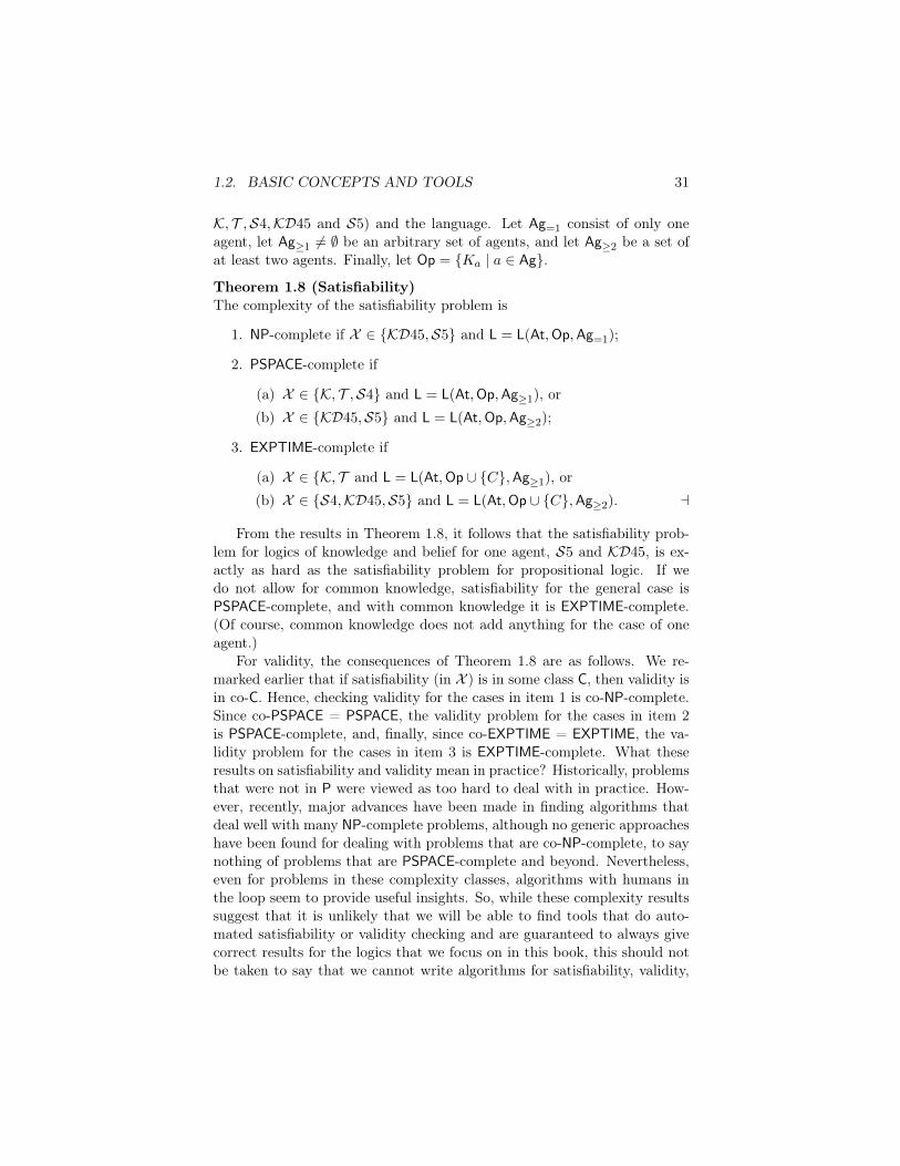
K, T , S4, KD45 and S5) and the language. Let Ag=1 consist of only oneagent, let Ag�1 6= ; be an arbitrary set of agents, and let Ag�2 be a set ofat least two agents. Finally, let Op = {Ka | a 2 Ag}.

Theorem 1.8 (Satisfiability)The complexity of the satisfiability problem is

1. NP-complete if X 2 {KD45, S5} and L = L(At,Op,Ag=1);

2. PSPACE-complete if

(a) X 2 {K, T , S4} and L = L(At,Op,Ag�1), or(b) X 2 {KD45, S5} and L = L(At,Op,Ag�2);

3. EXPTIME-complete if

(a) X 2 {K, T and L = L(At,Op [ {C},Ag�1), or(b) X 2 {S4, KD45, S5} and L = L(At,Op [ {C},Ag�2). a

From the results in Theorem 1.8, it follows that the satisfiability prob-lem for logics of knowledge and belief for one agent, S5 and KD45, is ex-actly as hard as the satisfiability problem for propositional logic. If wedo not allow for common knowledge, satisfiability for the general case isPSPACE-complete, and with common knowledge it is EXPTIME-complete.(Of course, common knowledge does not add anything for the case of oneagent.)

For validity, the consequences of Theorem 1.8 are as follows. We re-marked earlier that if satisfiability (in X ) is in some class C, then validity isin co-C. Hence, checking validity for the cases in item 1 is co-NP-complete.Since co-PSPACE = PSPACE, the validity problem for the cases in item 2is PSPACE-complete, and, finally, since co-EXPTIME = EXPTIME, the va-lidity problem for the cases in item 3 is EXPTIME-complete. What theseresults on satisfiability and validity mean in practice? Historically, problemsthat were not in P were viewed as too hard to deal with in practice. How-ever, recently, major advances have been made in finding algorithms thatdeal well with many NP-complete problems, although no generic approacheshave been found for dealing with problems that are co-NP-complete, to saynothing of problems that are PSPACE-complete and beyond. Nevertheless,even for problems in these complexity classes, algorithms with humans inthe loop seem to provide useful insights. So, while these complexity resultssuggest that it is unlikely that we will be able to find tools that do auto-mated satisfiability or validity checking and are guaranteed to always givecorrect results for the logics that we focus on in this book, this should notbe taken to say that we cannot write algorithms for satisfiability, validity,


or model checking that are useful for the problems of practical interest.Indeed, there is much work focused on just that.

1.2.5 Axiomatisation

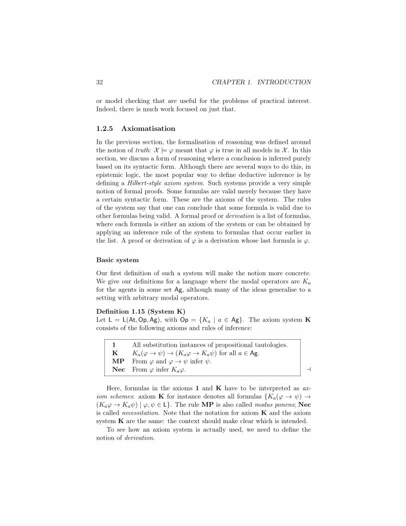
In the previous section, the formalisation of reasoning was defined aroundthe notion of truth: X |= ' meant that ' is true in all models in X . In thissection, we discuss a form of reasoning where a conclusion is inferred purelybased on its syntactic form. Although there are several ways to do this, inepistemic logic, the most popular way to define deductive inference is bydefining a Hilbert-style axiom system. Such systems provide a very simplenotion of formal proofs. Some formulas are valid merely because they havea certain syntactic form. These are the axioms of the system. The rulesof the system say that one can conclude that some formula is valid due toother formulas being valid. A formal proof or derivation is a list of formulas,where each formula is either an axiom of the system or can be obtained byapplying an inference rule of the system to formulas that occur earlier inthe list. A proof or derivation of ' is a derivation whose last formula is '.

Basic system

Our first definition of such a system will make the notion more concrete.We give our definitions for a language where the modal operators are Ka

for the agents in some set Ag, although many of the ideas generalise to asetting with arbitrary modal operators.

Definition 1.15 (System K)Let L = L(At,Op,Ag), with Op = {Ka | a 2 Ag}. The axiom system Kconsists of the following axioms and rules of inference:

1 All substitution instances of propositional tautologies.K Ka(' ! ) ! (Ka' ! Ka ) for all a 2 Ag.MP From ' and ' ! infer .Nec From ' infer Ka'. a

Here, formulas in the axioms 1 and K have to be interpreted as ax-iom schemes: axiom K for instance denotes all formulas {Ka(' ! ) !(Ka' ! Ka ) | ', 2 L}. The rule MP is also called modus ponens; Necis called necessitation. Note that the notation for axiom K and the axiomsystem K are the same: the context should make clear which is intended.

To see how an axiom system is actually used, we need to define thenotion of derivation.


Definition 1.16 (Derivation)Given a logical language L, let X be an axiom system with axioms Ax1, . . . ,Axn and rules Ru1, . . .Ruk. A derivation of ' in X is a finite sequence'1, . . . ,'m of formulas such that: (a) 'm = ', and (b) every 'i in thesequence is either an instance of an axiom or else the result of applying arule to formulas in the sequence prior to 'i. For the rules MP and Nec,this means the following:

MP 'h = 'j ! 'i, for some h, j < i.

That is, both 'j and 'j ! 'i occur in th sequence before 'i.

Nec 'i = Ka'j , for some j < i;

If there is a derivation for ' in X we write X ` ', or `X ', or, if the systemX is clear from the context, we just write ` '. We then also say that ' isa theorem of X, or that X proves '. The sequence '1, . . . ,'m is then alsocalled a proof of ' in X. a

Example 1.6 (Derivation in K)We first show that

K ` Ka(' ^ ) ! (Ka' ^ Ka ). (1.3)

We present the proof as a sequence of numbered steps (so that the formula'i in the derivation is given number i). This allows us to justify each stepin the proof by describing which axioms, rules of inference, and previoussteps in the proof it follows from.1. (' ^ ) ! ' 12. Ka((' ^ ) ! ') Nec, 13. Ka((' ^ ) ! ') ! (Ka(' ^ ) ! Ka') K4. Ka(' ^ ) ! Ka' MP, 2, 35. (' ^ ) ! 16. Ka((' ^ ) ! ) Nec, 57. Ka((' ^ ) ! ) ! (Ka(' ^ ) ! Ka ) K8. Ka(' ^ ) ! Ka MP, 6, 79. (Ka(' ^ ) ! Ka') !

((Ka(' ^ ) ! Ka ) ! (Ka(' ^ ) ! (Ka' ^ Ka ))) 110. (Ka(' ^ ) ! Ka ) ! (Ka(' ^ ) ! (Ka' ^ Ka )) MP, 4, 911. Ka(' ^ ) ! (Ka' ^ Ka ) MP, 8, 10

Lines 1, 5, and 9 are instances of propositional tautologies (this can bechecked using a truth table). Note that the tautology on line 9 is of theform (↵ ! �) ! ((↵ ! �) ! (↵ ! (� ^ �))). A proof like that abovemay look cumbersome, but it does show what can be done using only the


axioms and rules of K. It is convenient to give names to properties thatare derived, and so build a library of theorems. We have, for instance thatK ` KCD, where KCD (‘K-over-conjunction-distribution’) is

KCD Ka(↵ ^ �) ! Ka↵ and Ka(↵ ^ �) ! Ka�.

The proof of this follows steps 1 - 4 and steps 5 - 8, respectively, of theproof above. We can also derive new rules; for example, the following rule:CC (‘combine conclusions’) is derivable in K:

CC from ↵ ! � and ↵ ! � infer ↵ ! (� ^ �).

The proof is immediate from the tautology on line 9 above, to which wecan, given the assumptions, apply modus ponens twice. We can give a morecompact proof of Ka(' ^ ) ! (Ka' ^ Ka ) using this library:

1. Ka(' ^ ) ! Ka' KCD2. Ka(' ^ ) ! Ka KCD3. Ka(' ^ ) ! (Ka' ^ Ka ) CC, 1, 2 a

For every class X of models introduced in the previous section, we wantto have an inference system X such that derivability in X and validity inX coincide:

Definition 1.17 (Soundness and Completeness)Let L be a language, let X be a class of models, and let X be an axiomsystem. The axiom system is said to be

1. sound for X and the language L if, for all formulas ' 2 L, X ` 'implies X |= '; and

2. complete for X and the language L if, for all formulas ' 2 L, X |= 'implies X ` '.

We now provide axioms that characterize some of the subclasses of modelsthat were introduced in Definition 1.7.

Definition 1.18 (More axiom systems)Consider the following axioms, which apply for all agents a 2 Ag:

T. Ka' ! 'D. Ma>B. ' ! KaMa'4. Ka' ! KaKa'5. ¬Ka' ! Ka¬Ka'


A simple way to denote axiom systems is just to add the axioms that areincluded together with the name K. Thus, KD is the axiom system thathas all the axioms and rules of the system K (1, K, and rules MP andNec) together with D. Similarly, KD45 extends K by adding the axiomsD, 4 and 5. System S4 is the more common way of denoting KT4, whileS5 is the more common way of denoting KT45. If it is necessary to makeexplicit that there are m agents in Ag, we write Km, KDm, and so on. a

Using S5 to model knowledge

The system S5 is an extension of K with the so-called ‘properties of know-ledge’. Likewise, KD45 has been viewed as characterizing the ‘propertiesof belief’. The axiom T expresses that knowledge is veridical: whatever oneknows, must be true. (It is sometimes called the truth axiom.) The othertwo axioms specify so-called introspective agents: 4 says that an agent knowswhat he knows (positive introspection), while 5 says that he knows what hedoes not know (negative introspection). As a side remark, we mention thataxiom 4 is superfluous in S5; it can be deduced from the other axioms.

All of these axioms are idealisations, and indeed, logicians do not claimthat they hold for all possible interpretations of knowledge. It is only hu-man to claim one day that you know a certain fact, only to find yourselfadmitting the next day that you were wrong, which undercuts the axiomT. Philosophers use such examples to challenge the notion of knowledgein the first place (see the notes at the end of the chapter for references tothe literature on logical properties of knowledge). Positive introspectionhas also been viewed as problematic. For example, consider a pupil who isasked a question ' to which he does not know the answer. It may well bethat, by asking more questions, the pupil becomes able to answer that ' istrue. Apparently, the pupil knew ', but was not aware he knew, so did notknow that he knew '.

The most debatable among the axioms is that of negative introspection.Quite possibly, a reader of this chapter does not know (yet) what Moore’sparadox is (see Chapter 6), but did she know before picking up this bookthat she did not know that?

Such examples suggest that a reason for ignorance can be lack of aware-ness. Awareness is the subject of Chapter 3 in this book. Chapter 2 also hasan interesting link to negative introspection: this chapter tries to capturewhat it means to claim ‘All I know is '’; in other words, it tries to givean account of ‘minimal knowledge states’. This is a tricky concept in thepresence of axiom 5, since all ignorance immediately leads to knowledge!

One might argue that ‘problematic’ axioms for knowledge should just beomitted, or perhaps weakened, to obtain an appropriate system for know-


ledge, but what about the basic principles of modal logic: the axiom K andthe rule of inference Nec. How acceptable are they for knowledge? As onemight expect, we should not take anything for granted. K assumes perfectreasoners, who can infer logical consequences of their knowledge. It implies,for instance, that under some mild assumptions, an agent will know whatday of the week July 26, 5018 will be. All that it takes to answer this ques-tion is that (1) the agent knows today’s date and what day of the week it istoday, (2) she knows the rules for assigning dates, computing leap years, andso on (all of which can be encoded as axioms in an epistemic logic with theappropriate set of primitive propositions). By applying K to this collectionof facts, it follows that the agent must know what day of the week it will beon July 26, 5018. Necessitation assumes agents can infer all S5 theorems:agent a, for instance, would know that Kb(Kbq ^¬Kb(p ! ¬Kbq)) is equiv-alent to (Kbq^Mbp). Since even telling whether a formula is propositionallyvalid is co-NP-complete, this does not seem so plausible.

The idealisations mentioned in this paragraph are often summarised aslogical omniscience: our S5 agent would know everything that is logicallydeducible. Other manifestations of logical omniscience are the equivalenceof K(' ^ ) and K' ^ K , and the derivable rule in K that allows oneto infer K' ! K from ' ! (this says that agents knows all logicalconsequences of their knowledge).

The fact that, in reality, agents are not ideal reasoners, and not logi-cally omniscient, is sometimes a feature exploited by computational systems.Cryptography for instance is useful because artificial or human intrudersare, due to their limited capacities, not able to compute the prime factorsof a large number in a reasonable amount of time. Knowledge, security, andcryptographic protocols are discussed in Chapter 12

Despite these problems, the S5 properties are a useful idealisation ofknowledge for many applications in distributed computing and economics,and have been shown to give insight into a number of problems. The S5properties are reasonable for many of the examples that we have alreadygiven; here is one more. Suppose that we have two processors, a and b, andthat they are involved in computations of three variables, x, y, and z. Forsimplicity, assume that the variables are Boolean, so that they are either 0or 1. Processor a can read the value of x and of y, and b can read y and z.To model this, we use, for instance, 010 as the state where x = 0 = z, andy = 1. Given our assumptions regarding what agents can see, we then havex1y1z1 ⇠a x2y2z2 iff x1 = x2 and y1 = y2. This is a simple manifestation ofan interpreted system, where the accessibility relation is based on what anagent can see in a state. Such a relation is an equivalence relation. Thus, aninterpreted system satisfies all the knowledge axioms. (This is formalisedin Theorem 1.9(1) below.)


While T has traditionally been considered an appropriate axiom forknowledge, it has not been considered appropriate for belief. To reasonabout belief, T is typically replaced by the weaker axiom D: ¬Ba?, whichsays that the agent does not believe a contradiction; that is, the agent’sbeliefs are consistent. This gives us the axiom system KD45. We canreplace D by the following axiom D0 to get an equivalent axiomatisation ofbelief:

D0 : Ka' ! ¬Ka¬'.

This axioms says that the agent cannot know (or believe) both a fact andits negation. Logical systems that have operators for both knowledge andbelief often include the axiom Ka' ! Ba', saying that knowledge entailsbelief.

Axiom systems for group knowledge

If we are interested in formalising the knowledge of just one agent a, thelanguage L(At, {Ka},Ag) is arguably too rich. In the logic S51 it can beshown that every formula is equivalent to a depth-one formula, which hasno nested occurrences of Ka. This follows from the following equivalences,all of which are valid in S5 as well as being theorems of S5: KK' $ K';K¬K' $ ¬K'; K(K'_ ) $ (K'_K ); and K(¬K'_ ) $ ¬K'_K .From a logical perspective things become more interesting in the multi-agentsetting.

We now consider axiom systems for the notions of group knowledge thatwere defined earlier. Not surprisingly, we need some additional axioms.

Definition 1.19 (Logic of common knowledge)The following axiom and rule capture common knowledge.

Fix. CA' ! EA(' ^ CA').Ind. From ' ! EA( ^ ') infer ' ! CA .

For each axiom system X considered earlier, let XC be the result of addingFix and Ind to X. a

The fixed point axiom Fix says that common knowledge can be viewedas the fixed point of an equation: common knowledge of ' holds if everyoneknows both that ' holds and that ' is common knowledge. Ind is called theinduction rule; it can be used to derive common knowledge ‘inductively’.If it is the case that ' is ‘self-evident’, in the sense that if it is true, theneveryone knows it, and, in addition, if ' is true, then everyone knows , wecan show by induction that if ' is true, then so is Ek

A( ^ ') for all k. It


follows that CA' is true as well. Although common knowledge was definedas an ‘infinitary’ operator, somewhat surprisingly, these axioms completelycharacterize it.

For distributed knowledge, we consider the following axioms for all A ✓Ag:

W. Ka' ! DA' if a 2 A.KD. DA(' ! ) ! (DA' ! DA ).TD. DA' ! '.DD. ¬DA¬>.BD. ' ! DA¬DA¬'.4D. DA' ! DADA'.5D. ¬DA' ! DA¬DA'.

These axioms have to be understood as follows. It may help to think aboutdistributed knowledge in a group A as the knowledge of a wise man, whohas been told, by every member of A, what each of them knows. This iscaptured by axiom W. The other axioms indicate that the wise man hasat least the same reasoning abilities as distributed knowledge to the systemS5m, we add the axioms W,KD,TD,4D, and 5D to the axiom system. ForKm, we add only W and KD.

Proving Completeness

We want to prove that the axiom systems that we have defined are soundand complete for the corresponding semantics; that is, that K is sound andcomplete with respect to K, S5 is sound and complete with respect to S5,and so on. Proving soundness is straightforward: we prove by induction onk that any formula proved using a derivation of length k is valid. Provingcompleteness is somewhat harder. There are different approaches, but thecommon one involves to show that if a formula is not derivable, then thereis a model in which it is false. There is a special model called the canonicalmodel that simultaneously shows this for all formulas. We now sketch theconstruction of the canonical model.

The states in the canonical model correspond to maximal consistent setsof formulas, a notion that we define next. These sets provide the bridgebetween the syntactic and semantic approach to validity.

Definition 1.20 (Maximal consistent set)A formula ' is consistent with axiom system X if we cannot derive ¬' in X.A finite set {'1, . . . ,'n} of formulas is consistent with X if the conjunction'1^ . . .^'n is consistent with X. An infinite set � of formulas is consistentwith X if each finite subset of � is consistent with X. Given a language L


and an axiom system X, a maximal consistent set for X and L is a set � offormulas in L that is consistent and maximal, in the sense that every strictsuperset �0 of � is inconsistent. a

We can show that a maximal consistent set � has the property that, forevery formula ' 2 L, exactly one of ' and ¬' is in �. If both were in �, then� would be inconsistent; if neither were in �, then � would not be maximal.A maximal consistent set is much like a state in a Kripke model, in thatevery formula is either true or false (but not both) at a state. In fact, as wesuggested above, the states in the canonical model can be identified withmaximal consistent sets.Definition 1.21 (Canonical model)The canonical model for L and X is the Kripke model M = hS, R, V i definedas follows:

• S is the set of all maximal consistent sets for X and L;

• �Ra� iff �|Ka ✓ �, where �|Ka = {' | Ka' 2 �};

• V (�)(p) = true iff p 2 �. aThe intuition for the definition of Ra and V is easy to explain. Our

goal is to show that the canonical model satisfies what is called the TruthLemma: a formula ' is true at a state � in the canonical model iff ' 2 �.(Here we use the fact that the states in the canonical model are actually setsof formulas—indeed, maximal consistent sets.) We would hope to prove thisby induction. The definition of V ensures that the Truth Lemma holds forprimitive propositions. The definition of Ra provides a necessary conditionfor the Truth Lemma to hold for formulas of the form Ka'. If Ka' holds ata state (maximal consistent set) � in the canonical model, then ' must holdat all states � that are accessible from �. This will be the case if �|Ka ✓ �for all states � that are accessible from � (and the Truth Lemma appliesto ' and �).

The Truth Lemma can be shown to hold for the canonical model, aslong as we consider a language that does not involve common knowledgeor distributed knowledge. (The hard part comes in showing that if ¬Ka'holds at a state �, then there is an accessible state � such that ¬' 2 �.That is, we must show that the Ra relation has ‘enough’ pairs.) In additionto the Truth Lemma, we can also show that the canonical model for axiomsystem X is a model in the corresponding class of models; for example, thecanonical model for S5 is in S5.

Completeness follows relatively easily once these two facts are estab-lished. If a formula ' 2 L cannot be derived in X then ¬' must be con-sistent with X, and thus can be shown to be an element of a maximal


consistent set, say �. � is a state in the canonical model for X and L. Bythe Truth Lemma, ¬' is true at �, so there is a model where ' is false,proving the completeness of X.

This argument fails if the language includes the common knowledgeoperator. The problem is that with the common knowledge operator in thelanguage, the logic is not compact : there is a set of formulas such that allits finite subsets are satisfiable, yet the whole set is not satisfiable. Considerthe set {En

Ap | n 2 N} [ {¬CAp}, where A ✓ Ag is a group with at leasttwo agents. Each finite subset of this set is easily seen to be satisfiable ina model in S5 (and hence in a model in any of the other classes we haveconsidered), but the whole set of formulas is not satisfiable in any Kripkemodel. Similarly, each finite subset of this set can be shown to be consistentwith S5C. Hence, by definition, the whole set is consistent with S5C (andhence all other axiom systems we have considered). This means that thisset must be a subset of a maximal consistent set. But, as we have observed,there is no Kripke model where this set of formulas is satisfied.

This means that a different proof technique is necessary to prove com-pleteness. Rather than constructing one large canonical model for all for-mulas, for each formula ', we construct a finite canonical model tailored to'. And rather than considering maximal consistent subsets to the set of allformulas in the language, we consider maximal consistent sets of the set ofsubformulas of '.

The canonical model M' = hS', R, V i for ' and KC is defined asfollows:

• S' is the set of all maximal consistent sets of subformulas of ' forKC;

• �Ra� iff (�|Ka) [ {CA | CA 2 � and a 2 A} ✓ �.

• V (�)(p) = true iff p 2 �.

The intuition for the modification to the definition of Ra is the following:Again, for the Truth Lemma to hold, we must have �|Ka ✓ �, since ifKa 2 �, we want to hold in all states accessible from �. By the fixedpoint axiom, if CA is true at a state s, so is EACA ; moreover, if a 2 A,then KaCA is also true at s. Thus, if CA is true at �, CA must alsobe true at all states accessible from �, so we must have {CA | CA 2 �and a 2 A} ✓ �. Again, we can show that the Truth Lemma holds forthe canonical model for ' and KC for subformulas of '; that is, if is asubformula of ', then is true at a state � in the canonical model for 'and KC iff ' 2 �.

We must modify this construction somewhat for axiom systems thatcontain the axiom 4 and/or 5. For axiom systems that contain 4, we redefine


Ra so that �Ra� iff (� | Ka) [ {CA | CA 2 � and a 2 A} [ {Ka |Ka 2 �} ✓ �. The reason that we want {Ka' | Ka' 2 �} ✓ � is that ifKa is true at the state �, so is KaKa , so Ka must be true at all worldsaccessible from �. An obvious question to ask is why we did not make thisrequirement in our original canonical model construction. If both Ka andKaKa are subformulas of ', then the requirement is in fact not necessary.For if Ka 2 �, then consistency will guarantee that KaKa is as well, sothe requirement that �|Ka ✓ � guarantees that Ka 2 �. However, ifKa is a subformula of ' but KaKa is not, this argument fails.

For systems that contain 5, there are further subtleties. We illustratethis for the case of S5. In this case, we require that �Ra� iff {Ka | Ka 2�} = {Ka | Ka 2 �} and {CA | CA 2 � and a 2 A} = {CA | CA 2� and a 2 A}. Notice that the fact that {Ka | Ka 2 �} = {Ka | Ka 2�} implies that �|Ka = �|Ka. We have already argued that having 4 in thesystem means that we should have {Ka | Ka 2 �} ✓ {Ka | Ka 2 �}.For the opposite inclusion, note that if Ka /2 �, then ¬Ka should be trueat the state � in the canonical model, so (by 5) Ka¬Ka is true at �, and¬Ka is true at � if �Ra�. But this means that Ka /2 � (assuming thatthe Truth Lemma applies). Similar considerations show that we must have{CA | CA 2 � and a 2 A} = {CA | CA 2 � and a 2 A}, using thefact that ¬CA ! EA¬CA is provable in S5C.

Getting a complete axiomatisation for languages involving distributedknowledge requires yet more work; we omit details here.

We summarise the main results regarding completeness of epistemic lo-gics in the following theorem. Recall that, for an axiom system X, the axiomsystem XC is the result of adding the axioms Fix and Ind to X. Similarly,XD is the result of adding the ‘appropriate’ distributed knowledge axiomsto X; specifically, it includes the axiom W, together with every axiom YD

for which Y is an axiom of X. So, for example, S5D has the axioms of S5together with W, KD, TD, 4D, and 5D.

Theorem 1.9If (At,Op,Ag), X is an axiom systems that includes all the axioms andrules of K and some (possibly empty) subset of {T,4,5,D}, and X is thecorresponding class of Kripke models, then the following hold:

1. if Op = {Ka | a 2 Ag}, then X is sound and complete for X and L;

2. if Op = {Ka | a 2 Ag} [ {CA | A ✓ Ag}, then XC is sound andcomplete for X and L;

3. if Op = {Ka | a 2 Ag} [ {DA | A ✓ Ag}, then XD is sound andcomplete for X and L;


4. if Op = {Ka | a 2 Ag} [ {CA | A ✓ Ag} [ {DA | A ✓ Ag}, then XCDis sound and complete for X and L. a

1.3 Overview of the Book

The book is divided into three parts: informational attitudes, dynamics,and applications. Part I, informational attitudes, considers ways that basicepistemic logic can be extended with other modalities related to knowledgeand belief, such as “only knowing”, “awareness”, and probability. There arethree chapters in Part I:

Only Knowing Chapter 2, on only knowing, is authored by GerhardLakemeyer and Hector J. Levesque. What do we mean by ‘only knowing’?When we say that an agent knows p, we usually mean that the agent knowsat least p, but possibly more. In particular, knowing p does not allow usto conclude that q is not known. Contrast this with the situation of aknowledge-based agent, whose knowledge base consists of p, and nothingelse. Here we would very much like to conclude that this agent does notknow q, but to do so requires us to assume that p is all that the agent knowsor, as one can say, the agent only knows p. In this chapter, the logic of onlyknowing for both single and multiple agents is considered, from both thesemantic and proof-theoretic perspective. It is shown that only knowingcan be used to capture a certain form of honesty, and that it relates to aform of non-monotonic reasoning.

Awareness Chapter 3, on logics where knowledge and awareness interact,is authored by Burkhard Schipper. Roughly speaking, an agent is unawareof a formula ' if ' is not on his radar screen (as opposed to just havingno information about ', or being uncertain as to the truth of '). Thechapter discusses various approaches to modelling (un)awareness. Whilethe focus is on axiomatisations of structures capable of modelling knowledgeand awareness, structures for modelling probabilistic beliefs and awareness,are also discussed, as well as structures for awareness of unawareness.

Epistemic Probabilistic Logic Chapter 4, authored by Lorenz Demeyand Joshua Sack, provides an overview of systems that combine probabilitytheory, which describes quantitative uncertainty, with epistemic logic, whichdescribes qualitative uncertainty. By combining knowledge and probability,one obtains a very powerful account of information and information flow.Three types of systems are investigated: systems that describe uncertainty

1.3. OVERVIEW OF THE BOOK 43

of agents at a single moment in time, systems where the uncertainty changesover time, and systems that describe the actions that cause these changes.

Part II on dynamics of informational attitudes considers aspects of howknowledge and belief change over time. It consists of three chapters:

Knowledge and Time Chapter 5, on knowledge and time, is authoredby Clare Dixon, Cláudia Nalon, and Ram Ramanujam. It discusses thedynamic aspects of knowledge, which can be characterized by a combina-tion of temporal and epistemic logics. The chapter presents the languageand axiomatisation for such a combination, and discusses complexity andexpressivity issues. It presents two different proof methods (which applyquite broadly): resolution and tableaux. Levels of knowledge and the re-lation between knowledge and communication in distributed protocols arealso discussed, and an automata-theoretic characterisation of the knowledgeof finite-state agents is provided. The chapter concludes with a brief surveyon applications.

Dynamic Epistemic Logic Chapter 6, on dynamic epistemic logic, isauthored by Lawrence Moss. Dynamic Epistemic Logic (DEL) extendsepistemic logic with operators corresponding to epistemic actions. The mostbasic epistemic action is a public announcement of a given sentence to allagents. In the first part of the chapter, a logic called PAL (public announce-ment logic), which includes announcement operators, is introduced. Fourdifferent axiomatisations for PAL are given and compared. It turns outthat PAL without common knowledge is reducible to standard epistemiclogic: the announcement operators may be translated away. However, thischanges once we include common knowledge operators in the language. Thesecond part of Chapter 6 is devoted to more general epistemic actions, suchas private announcements.

Dynamic Logics of Belief Change Chapter 7, on belief change, is au-thored by Johan van Benthem and Sonja Smets. The chapter gives anoverview of current dynamic logics that describe belief update and revision.This involves a combination of ideas from belief revision theory and dynamicepistemic logic. The chapter describes various types of belief change, de-pending on whether the information received is ‘hard’ or ‘soft’. The chaptercontinues with three topics that naturally complement the setting of singlesteps of belief change: connections with probabilistic approaches to beliefchange, long-term temporal process structure including links with formallearning theory, and multi-agent scenarios of information flow and belief re-


vision in games and social networks. It ends with a discussion of alternativeapproaches, further directions, and windows to the broader literature.

Part III considers applications of epistemic logic in various areas. It consistsof five chapters:

Model Checking Temporal Epistemic Logic Chapter 8, authoredby Alessio Lomuscio and Wojciech Penczek, surveys work on model check-ing systems against temporal-epistemic specifications. The focus is on twoapproaches to verification: approaches based on ordered binary decisiondiagrams (OBDDs) and approaches based on translating specifications topropositional logic, and then applying propositional satisfiability checkers(these are called SAT-based approaches). OBDDs provide a compact rep-resentation for propositional formulas; they provide powerful techniques forefficient mode checking; SAT-based model checking is the basis for manyrecent symbolic approach to verification. The chapter also discusses somemore advanced techniques for model checking.

Epistemic Foundations of Game Theory Chapter 9, authored by Gi-acomo Bonanno, provides an overview of the epistemic approach to gametheory. Traditionally, game theory focuses on interaction among intelligent,sophisticated and rational individuals. The epistemic approach attemptsto characterize, using epistemic notions, the behavior of rational and intel-ligent players who know the structure of the game and the preferences oftheir opponents and who recognize each other’s rationality and reasoningabilities. The focus of the analysis is on the implications of common beliefof rationality in strategic-form games and on dynamic games with perfectinformation.

BDI Logics Chapter 10, on logics of beliefs, desires, and intentions (BDI),is authored by John-Jules Ch. Meyer, Jan Broersen and Andreas Herzig.Various formalisations of BDI in logic are considered, such as the approachof Cohen and Levesque (recast in dynamic logic), Rao and Georgeff’s in-fluential BDI logic based on the branching-time temporal logic CTL⇤, theKARO framework, in which action together with knowledge (or belief) isthe primary concept on which other agent notions are built, and BDI logicsbased on STIT (seeing to it that) logics, such as XSTIT.

Knowledge and Ability Chapter 11, authored by Thomas Ågotnes,Valentin Goranko, Wojciech Jamroga and Michael Wooldridge, relates epis-temic logics to various logics for strategic abilities. It starts by discussing

1.4. NOTES 45

approaches from philosophy and artificial intelligence to modelling the in-teraction of agents knowledge and abilities, and then focuses on concurrentgame models and the alternating-time temporal logic ATL. The authorsdiscuss how ATL enables reasoning about agents’ coalitional abilities toachieve qualitative objectives in concurrent game models, first assumingcomplete information and then under incomplete information and uncer-tainty about the structure of the game model. Finally, extensions of ATLthat allow explicit reasoning about the interaction of knowledge and strate-gic abilities are considered; this leads to the notion of constructive know-ledge.

Knowledge and Security Chapter 12, on knowledge and security, is au-thored by Riccardo Pucella. A persistent intuition in the field of computersecurity says that epistemic logic, and more generally epistemic concepts,are relevant to the formalisation of security properties. What grounds thisintuition is that much work in the field is based on epistemic concepts.Confidentiality, integrity, authentication, anonymity, non-repudiation, allcan be expressed as epistemic properties. This survey illustrates the useof epistemic concepts and epistemic logic to formalise a specific securityproperty, confidentiality. Confidentiality is a prime example of the use ofknowledge to make a security property precise. It is explored in two largedomains of application: cryptographic protocol analysis and multi-level se-curity systems.

1.4 Notes

The seminal work of the philosopher Jaakko Hintikka (1962) is typicallytaken as the starting point of modern epistemic logic. Two texts on epis-temic logic by computer scientists were published in 1995: one by Fagin,Halpern, Moses, and Vardi (1995) and the other by Meyer and van der Hoek(1995). Another influential text on epistemic logic, which focuses more onphilosophical aspects, is by Rescher (2005). Formal treatments of the no-tion of knowledge in artificial intelligence, in particular for reasoning aboutaction, go back to the work of Moore (1977). In the mid-1980s, the con-ference on Theoretical Aspects of Reasoning About Knowledge (TARK),later renamed to “Theoretical Aspects of Rationality and Knowledge, wasstarted (1986); in the mid-1990s, the Conference on Logic and Foundationsof Game and Decision Theory (LOFT) (1996) began. These two conferencescontinue to this day, bringing together computer scientists, economists, andphilosophers.

Our chapter is far from the first introduction to epistemic logic. The


textbooks by Fagin et al. (1995) and by Meyer and van der Hoek (1995) eachcome with an introductory chapter; more recent surveys and introductionscan be found in the book by van Ditmarsch, van der Hoek, and Kooi (2007,Chapter 2), in a paper on epistemic logic and epistemology by Holliday(2014), in the chapter by Bezhanishvili and van der Hoek (2014), whichprovides a survey of semantics for epistemic notions, and in online resources(Hendricks and Symons 2014, Wikipedia).

Halpern (1987) provides an introduction to applications of knowledgein distributed computing; the early chapters of the book by Perea (2012)give an introduction to the use of epistemic logic in game theory. As wealready said, more discussion of the examples in Section 1.1 can be found inthe relevant chapters. Public announcements are considered in Chapter 6;protocols are studied in Chapter 12 and, to some extent, in Chapter 5;strategic ability is the main topic of Chapter 11; epistemic foundations ofgame theory are considered in Chapter 9; distributed computing is touchedon in Chapter 5, while examples of model checking distributed protocolsare given in Chapter 8.

The use of Kripke models puts our approach to epistemic logic firmlyin the tradition of modal logic, of which Kripke is one of the founders (seeKripke (1963)). Modal logic has become the framework to reason not onlyabout notions as knowledge and belief, but also about agent attitudes suchas desires and intentions (Rao and Georgeff, 1991), and about notions liketime (Emerson, 1990), action (Harel, 1984), programs (Fischer and Ladner,1979), reasoning about obligation and permission (von Wright, 1951), andcombinations of them. Modern references to modal logic include the text-book by Blackburn, de Rijke, and Venema (2001) and the handbook editedby Blackburn, van Benthem, and Wolter (2006).

Using modal logic to formalise knowledge and belief suggests that onehas an idealised version of these notions in mind. The discussion in Sec-tion 1.2.5 is only the tip of the iceberg. Further discussion of logical omni-science can be found in (Stalnaker, 1991; Sim, 1997) and in (Fagin et al.,1995, Chapter 9). There is a wealth of discussion in the philosophy andpsychology literature of the axioms and their reasonableness (Koriat, 1993;Larsson, 2004; Zangwill, 2013). Perhaps the most controversial axiom ofknowledge is 5; which was dismissed in the famous claim by Donald Rums-feld that there are ‘unknown unknowns’ (see http://en.wikipedia.org/

wiki/There_are_known_knowns). Some approaches for dealing with lack ofknowledge using awareness avoid this axiom (and, indeed, all the others);see Chapter 3.

Broadly speaking, philosophers usually distinguish between the truthof a claim, our belief in it, and the justification for the claim. These areoften considered the three key elements of knowledge. Indeed, there are

1.4. NOTES 47

papers that define knowledge as justified true belief. There has been muchdebate of this definition, going back to Gettier’s (1963) Is justified true beliefknowledge?. Halpern, Samet, and Segev (2009) provide a recent perspectiveon these issues.

The notion of common knowledge is often traced back to the philoso-pher David Lewis’s (1969) independently developed by the sociologist Mor-ris Friedell (1969). Work on common knowledge in economics was initiatedby Robert Aumann (1976); John McCarthy’s (1990) work involving com-mon knowledge had a significant impact in the field of artificial intelligence.Good starting points for further reading on the topic of common knowledgeare by Vanderschraaf and Sillari (2014) and by Fagin et al. (1995, Chapter6). Section 9.5 compares the notions of common knowledge with that ofcommon belief.

Distributed knowledge was discussed first, in an informal way, by Hayek(1945), and then, in a more formal way, by Hilpinen (1977). It was rediscov-ered and popularized by Halpern and Moses (1990), who originally calledit implicit knowledge.

The notion of bisimulation is a central notion in modal logic, providingan answer to the question when two models are ‘the same’ and is discussedin standard modal logic texts (Blackburn et al., 2001, 2006). Bisimulationarises quite often in this book, including in Chapters 5, 6, and 7.

We mentioned below Theorem 1.8, when discussing complexity of va-lidity, that some recent advances make NP-complete problems seem moretractable: for this we refer to work by Gomes, Kautz, Sabharwal, and Sel-man (2008).

We end this brief discussion of the background literature by providingthe pointers to the technical results mentioned in our chapter. Theorem 1.1gives some standard valid formulas for several classes of models (see Faginet al. (1995, Chapter 2.4) for a textbook treatment). Theorem 1.2 is afolk theorem in modal logic: for a proof and discussion, see Blackburn et al.(2006, Chapter 2.3). Proposition 1.3 is proved by Fagin et al. (1995) as The-orem 3.2.2 (for the case X = K) and Theorem 3.2.4 (for X = T , S4, KD45,and S5). Proposition 1.4 is Proposition 3.2.1 by Fagin et al. (1995). Theo-rem 1.8 is proved by Halpern and Moses (1992).

Although the first proofs of completeness for multi-agent versions of ax-iom systems of the form Xm and XCm are by Halpern and Moses (1992),the ideas go back much earlier. In particular, the basic canonical model con-struction goes back to Makinson (1966) (see Blackburn et al. (2001, Chapter4) for a discussion), while the idea for completeness of axiom systems of theform XC is already in the proof of Kozen and Parikh (1981) for provingcompleteness of dynamic logic. Completeness for axiom systems of the formXD was proved by Fagin, Halpern, and Vardi (1992) and by van der Hoek


and Meyer (1992). A novel proof is provided by Wang (2013, Chapter 3).Theorem 1.6 is part of logical folklore. A proof of Theorem 1.7 was givenby French, van der Hoek, Iliev, and Kooi (2013).

Acknowledgements The authors are indebted to Cláudia Nalon for acareful reading. Hans van Ditmarsch is also affiliated to IMSc, Chennai,as associated researcher, and he acknowledges support from European Re-search Council grant EPS 313360. Joseph Y. Halpern was supported in partby NSF grants IIS-0911036 and CCF-1214844, by AFOSR grant FA9550-09-1-0266, by ARO grants W911NF-09-1-0281 and W911NF-14-1-0017, and bythe Multidisciplinary University Research Initiative (MURI) program ad-ministered by the AFOSR under grant FA9550-12-1-0040.

49

ReferencesAumann, R. J. (1976). Agreeing to disagree. Annals of Statistics 4 (6), 1236–1239.

Bezhanishvili, N. and W. van der Hoek (2014). Structures for epistemic logic. InA. Baltag and S. Smets (Eds.), Logical and Informational Dynamics, a volumein honour of Johan van Benthem, pp. 339–381. Springer.

Blackburn, P., M. de Rijke, and Y. Venema (2001). Modal Logic. CambridgeUniversity Press: Cambridge, England.

Blackburn, P., J. van Benthem, and F. Wolter (Eds.) (2006). Handbook of ModalLogic. Elsevier Science Publishers B.V.: Amsterdam, The Netherlands.

van Ditmarsch, H., W. van der Hoek, and B. Kooi (2007). Dynamic EpistemicLogic. Berlin: Springer.

Emerson, E. A. (1990). Temporal and modal logic. In J. van Leeuwen (Ed.), Hand-book of Theoretical Computer Science Volume B: Formal Models and Semantics,pp. 996–1072. Elsevier Science Publishers B.V.: Amsterdam, The Netherlands.

Fagin, R., J. Y. Halpern, Y. Moses, and M. Y. Vardi (1995). Reasoning AboutKnowledge. The MIT Press: Cambridge, MA.

Fagin, R., J. Y. Halpern, and M. Y. Vardi (1992). What can machines know? onthe properties of knowledge in distributed systems. Journal of the ACM 39 (2),328–376.

Fischer, M. and R. Ladner (1979). Propositional dynamic logic of regular pro-grams. Journal of Computer and System Sciences 18, 194–211.

French, T., W. van der Hoek, P. Iliev, and B. Kooi (2013). On the succinctness ofsome modal logics. Artificial Intelligence 197, 56–85.

Friedell, M. (1969). On the structure of shared awareness. Behavioral Sci-ence 14 (1), 28–39. A working paper with the same title was published in 1967by the Center for Research on Social Organization, University of Michigan.

Gettier, E. (1963). Is justified true belief knowledge? Analysis 23, 121Ð123.

Gomes, C. P., H. Kautz, A. Sabharwal, and B. Selman (2008). Satisfiability solvers.In Handbook of Knowledge Representation, pp. 89–133.

Halpern, J. Y. (1987). Using reasoning about knowledge to analyze distributedsystems. In J. F. Traub, B. J. Grosz, B. W. Lampson, and N. J. Nilsson (Eds.),Annual Review of Computer Science, Volume 2, pp. 37–68. Palo Alto, Calif.:Annual Reviews Inc.

Halpern, J. Y. and Y. Moses (1990). Knowledge and common knowledge in adistributed environment. Journal of the ACM 37 (3), 549–587. A preliminaryversion appeared in Proc. 3rd ACM Symposium on Principles of DistributedComputing, 1984.


Halpern, J. Y. and Y. Moses (1992). A guide to completeness and complexity formodal logics of knowledge and belief. Artificial Intelligence 54, 319–379.

Halpern, J. Y., D. Samet, and E. Segev (2009). Defining knowledge in termsof belief: The modal logic perspective. The Review of Symbolic Logic 2 (3),469–487.

Harel, D. (1984). Dynamic logic. In D. Gabbay and F. Guenther (Eds.), Handbookof Philosophical Logic Volume II — Extensions of Classical Logic, pp. 497–604.D. Reidel Publishing Company: Dordrecht, The Netherlands. (Synthese libraryVolume 164).

Hayek, F. (1945). The use of knowledge in society. American Economic Review 35,519–530.

Hendricks, V. and J. Symons (retrieved 2014). Epistemic logic. In E. N. Zalta(Ed.), The Stanford Encyclopedia of Philosophy. http://plato.stanford.

edu/archives/spr2014/entries/logic-epistemic/.

Hilpinen, R. (1977). Remarks on personal and impersonal knowledge. CanadianJournal of Philosophy 7, 1–9.

Hintikka, J. (1962). Knowledge and Belief. Cornell University Press: Ithaca, NY.Reprint: ‘Knowledge and Belief’, in: Texts in Philosophy, Vol. 1, Kings CollegePublications, 2005.

van der Hoek, W. and J.-J. Meyer (1992). Making some issues of implicit knowledgeexplicit. International Journal of Foundations of Computer Science 3 (2), 193–224.

Holliday, W. (2014). Epistemic logic and epistemology. to appear, preliminaryversion at http://philosophy.berkeley.edu/file/814/el_episteme.pdf.

Koriat, A. (1993). How do we know that we know? the accessibility model of thefeeling of knowing. Psychological review 100, 609Ð639.

Kozen, D. and R. Parikh (1981). An elementary proof of the completeness of PDL.Theoretical Computer Science 14 (1), 113–118.

Kripke, S. (1963). Semantical analysis of modal logic. Zeitschrift für Mathematis-che Logik und Grundlagen der Mathematik 9, 67–96.

Larsson, S. (2004). The magic of negative introspection.

Lewis, D. (1969). Convention — A Philosophical Study. Harvard University Press:Cambridge, MA.

LOFT (since 1996). Logic and the foundations of game and decision theory. http://www.econ.ucdavis.edu/faculty/bonanno/loft.html.

Makinson, D. (1966). On some completeness theorems in modal logic. Zeitschriftfür Mathematische Logik und Grundlagen der Mathematik 12, 379–384.

REFERENCES 51

McCarthy, J. (1990). Formalization of two puzzles involving knowledge. In V. Lif-schitz (Ed.), Formalizing Common Sense : Papers by John McCarthy, AblexSeries in Artificial Intelligence. Norwood, N.J.: Ablex Publishing Corporation.original manuscript dated 1978–1981.

Meyer, J.-J. C. and W. van der Hoek (1995). Epistemic Logic for AI and ComputerScience. Cambridge University Press: Cambridge, England.

Moore, R. C. (1977). Reasoning about knowledge and action. In Proceedings ofthe Fifth International Joint Conference on Artificial Intelligence (IJCAI-77),Cambridge, MA.

Perea, A. (2012). Epistemic Game Theory. Cambridge, U.K.: Cambridge Univer-sity Press.

Rao, A. S. and M. P. Georgeff (1991, April). Modeling rational agents within aBDI-architecture. In R. Fikes and E. Sandewall (Eds.), Proceedings of Know-ledge Representation and Reasoning (KR&R-91), pp. 473–484. Morgan Kauf-mann Publishers: San Mateo, CA.

Rescher, N. (2005). Epistemic Logic: A Survey of the Logic of Knowledge. Uni-versity of Pittsburgh Press.

Sim, K. M. (1997). Epistemic logic and logical omniscience: A survey. InternationalJournal of Intelligent Systems 12 (1), 57–81.

Stalnaker, R. (1991). The problem of logical omniscience, I. Synthese 89 (3),425–440.

TARK (since 1986). Theoretical aspects of rationality and knowledge. http:

//www.tark.org.

Vanderschraaf, P. and G. Sillari (retrieved 2014). Common knowledge. InE. N. Zalta (Ed.), The Stanford Encyclopedia of Philosophy. http://plato.

stanford.edu/archives/spr2014/entries/common-knowledge/.

Wang, Y. (2013). Logical Dynamics of Group Knowledge and Subset Spaces. Ph.D. thesis, University of Bergen.

Wikipedia. Epistemic modal logic. http://en.wikipedia.org/wiki/Epistemic_modal_logic.

von Wright, G. H. (1951). Deontic logic. Mind 60 (237), 1–15.

Zangwill, N. (2013). Does knowledge depend on truth? Acta Analytica 28 (2),139–144.

Documents

An Introduction to Logics of Knowledge and Belief - … · · 2015-02-20An Introduction to Logics of Knowledge and Belief Hans van Ditmarsch ... It turns out that, ... must ensure,