Embed Size (px)
Citation preview

Chemistry Learning Trends
An Introduction toKey Concepts in
Medicinal Chemistry
Elsevier’s Learning Trends Series

Contents
Cover image 1
Introduction 2
Chapter 3. Drug Targets, Target Identification,
Validation, and Screening 45
I Introduction 45
II What is a Drug Target? 46
III The Purpose of Target Identification 47
IV Target Options and Treatment Options 51
V Target Deconvolution and Target Discovery 53
VI Methods for Target Identification and Validation 54
VII Target Validation 68
VIII Conclusion 68
References 68
Medicinal and Pharmaceutical Chemistry 1
The Pre-Medicinal Chemistry Era 1
The Birth of the New Discipline 2
Medicinal Chemistry in the 20th Century; Some
Dreams Come True 2
Current Medicinal Chemistry; An Integrated
Interdisciplinary Branch of Chemistry 3
Comprehensive Medicinal Chemistry 4
References 5
Perspectives in Drug Discovery 1

Introduction 1
Case 1 1
Case 2 3
Case 3 3
References 4
LIQUID CHROMATOGRAPHY | Affinity Chromatography 1
Introduction 1
Basic Principles of Affinity Chromatography 1
Applications of Affinity Chromatography 5
Further Reading 8
3.05. Microarrays 87
3.05.1 Introduction 87
3.05.2 Deoxyribonucleic Acid Microarray Experiments 88
3.05.3 Data Analysis Considerations 91
3.05.4 Case Studies 93
3.05.5 Discussion and a Look to the Future 103
References 104
4.09. Systems Biology 279
4.09.1 Introduction 280
4.09.2 Study Setup 285
4.09.3 Data Preprocessing 290
4.09.4 Data Analysis 292
4.09.5 Metabolite Identification 299
4.09.6 Interpretation and Visualization 302
References 306
Comparative Modeling of Drug Target Proteins 1
Introduction 2

Steps in Comparative Modeling 2
Model Building 5
Refinement of Comparative Models 6
Errors in Comparative Models 7
Prediction of Model Errors 9
Evaluation of Comparative Modeling Methods 9
Applications of Comparative Models 10
Future Directions 12
Automation and Availability of Resources for
Comparative Modeling and Ligand Docking 13
References 16

Introduction
This volume is part of Elsevier’s Learning Trends series. Elsevier Science & Technology Books provides this series of free digital volumes to support and encourage learning and development across the sciences. Titles include content excerpts focused on a central theme to give the reader an introduction to new ideas and information on that topic.
This volume in Chemistry Learning Trends introduces readers to a key chapter from the 4th edition of Camille Wermuth’s Practice of Medicinal Chemistry and highlights the interdisciplinary nature of medicinal chemistry. The succeeding articles, from the ScienceDirect Reference Module in Chemistry, Molecular Sciences and Chemical Engineering, will introduce readers to important themes and valuable methods raised in this chapter.
Thank you for being a part of the Elsevier community!

C H A P T E R
3
Drug Targets, Target Identification, Validation,and Screening
Walter M.M. Van den BroeckJanssen Infectious Diseases BVBA, Beerse, Belgium
O U T L I N E
I. Introduction 45
II. What is a Drug Target? 46
III. The Purpose of Target Identification 47A. Target-Based Screening. 47B. Phenotypic Screening 47C. Fast Follower Strategy 50
IV. Target Options and Treatment Options 51
V. Target Deconvolution and Target Discovery 53
VI. Methods for Target Identification andValidation 54A. Affinity Chromatography 54B. Genetic Methods 57
C. Haploinsufficiency Profiling in Yeast 58D. Analysis of Resistant Mutants 59E. siRNA for Target Validation 60F. Yeast Three-Hybrid System 61G. DNA Microarrays 63H. Comparative Profiling 64I. Analysis of the Pathophysiology 65J. The Study of Existing Drugs 66K. Systems Biology 66L. In Silico Simulation of the Human Patient 67
VII. Target Validation 68
VIII. Conclusion 68
References 68
It doesn’t matter how beautiful your theory is, it doesn’t matter how smart you are or what your name is, if it doesn’t agreewith experiment, it’s wrong. Richard P. Feynman (American theoretical physicist 1918–1988)
I. INTRODUCTION
For ages, humans have been using medicinal substances without tools like DNA microarrays to identify them.Instead, they were guided by theories like the concept of the four humors in Greco-Roman medicine or by spiritual sys-tems like animism. The chances are high that modern medicinal chemists would fully reject these rationales. Today webelieve that the essential first step in the discovery of a new cure for a disease is the identification of the protein that isat the basis of that disease. The chances are high that medicinal chemists would fully agree with this rationale, butmaybe they shouldn’t. In this chapter, we will see why.
45The Practice of Medicinal Chemistry. © 2015 Elsevier Ltd. All rights reserved.

First, we examine why the definition of a drug target is already a bit misleading. Then we explore whether themantra “first a target, then a drug” is a good guideline. We compare the three most used strategies for drug dis-covery today and assess the role of target identification in these strategies. The next question is what kind of tar-gets we should try to identify. Is the search for the cause of a disease a fruitful road to find new cures? Can wefind cures altogether? Finally, after having established the difference between the two meanings of target identifi-cation, we describe briefly the current and most frequently used methods to identify and validate drug targets.
II. WHAT IS A DRUG TARGET?
In 1891, Paul Ehrlich was experimenting with dyes to stain bacteria. He had already made outstanding contribu-tions in treating infected patients with antitoxins. Together with vaccines, these account for the successful immuno-therapy. Ehrlich saw this immunotherapy as chemical reactions between very complex structures. At that time, theconcepts of cells and microorganisms were very new and nobody understood the composition of cells. Maybe acell was one big molecule, (i.e., a cell-molecule). Ehrlich believed that cell-molecules had side-chains to receivenutrients from outside, and he called these side-chains receptors. He thought that bacteria also had receptors andthat the staining of bacteria was a chemical reaction between the dye molecule and the receptors. What if this reac-tion could not only stain the bacteria but also kill them? What if this dye could do the same in an infected patient?Ehrlich showed that methylene blue was taken up by the malaria parasite and had modest effects in two patients.He was extremely excited by this and coined the term “chemotherapy.” The difference with immunotherapy wasthat now the antitoxins—which were very complex and difficult to produce and standardize—could be replacedby well-identified chemicals (small molecules) that were easier to produce and handle.
We owe the concept that a drug acts by binding to a target molecule to Paul Ehrlich. In his ownwords:,“Corpora non agunt nisi fixata” or “substances don’t act unless they are bound.” Today this concept isstill valid. The Oxford Dictionary of Biochemistry defines a drug target as “a biological entity (usually a protein orgene) that interacts with, and whose activity is modulated by, a particular compound.” Peter Imming [1] uses thefollowing working definition: a molecular structure (chemically definable by at least a molecular mass) that willundergo a specific interaction with chemicals we call drugs because they are administered to treat or diagnose adisease. The interaction has a connection with the clinical effect(s).
These definitions could give the misleading impression that a drug�target interaction is a one-to-one relation[2], as if every drug acted by binding to one and only one single specific target. This impression is furtherstrengthened by the ambition of every medicinal chemist, starting with Paul Erhlich himself, to synthesize a“magic bullet,” an ultra-specific compound that would bind only to the target and to nothing else. However, evi-dence is growing that many drugs are successful just because they act on multiple different—not co-located—targets, potentially even hitting several pathways together [3]. Of the 1366 drugs reported in DrugBank 2.0, about960 have more than one therapeutic target [4], a phenomenon called polypharmacology. As a consequence,searching for a super-selective drug may not always lead to the most active compound. In this perspective,target-based drug screening is not well suited to discover these so called “dirty drugs.”
The one-to-one relation also doesn’t fit with drugs that act by binding to a complex of proteins or even a com-plex between proteins and nucleic acids. Many proteins form dimers, trimers, or even more complex constella-tions. In these cases, the drug binding pocket could contain parts of two or more proteins. But the targetdiscovery tools are less well suited to find such targets.
Yet another—very obvious—violation of the one-to-one relation is that the same pocket can accommodatemany different small molecules. A substantial part of all new drugs is based on this promiscuous behavior ofmany pockets. The production of close analogues—or, more pejoratively, “me too drugs” —is often seen as a riskaverse and profit driven strategy. Nevertheless, these drugs often result in an important incremental progress inactivity, side effect profile, or administration facility [5].
A less obvious violation of the one-to-one relation is the fact that a protein can contain multiple pockets. Usuallythese pockets are all different and could partially overlap, be indirectly connected by allosteric regulation, or becompletely separated. The binding to these different pockets could result in different effects. For example, the bind-ing with nucleoside drugs to the active site of a viral polymerase makes it more difficult for the virus to build resis-tance than with nonnucleoside drugs that have their binding site outside the active site of the enzyme.
These comments make the picture of a drug target more complex. We could define a drug target as theminimal constellation of molecules that elicit a medically desired effect when bound by a drug.
46 3. DRUG TARGET IDENTIFICATION AND SCREENING
I. GENERAL ASPECTS OF MEDICINAL CHEMISTRY

III. THE PURPOSE OF TARGET IDENTIFICATION
Before exploring the plethora of methods to identify drug targets, we should discuss the role and the value oftarget identification in the drug discovery process. We will describe the role of target identification in the follow-ing three drug discovery strategies for small molecules:
� Target-Based Screening Strategy� Phenotypic Screening Strategy� Fast Follower Strategy
A. Target-Based Screening
Target identification is the cornerstone of target-based screening. The concept underlying this strategy is thatat the most fundamental level, most drugs work by binding to a specific target. Therefore, if you want to make atruly new drug, the first thing you have to do is to find a new target. The next step is to find small moleculesthat bind to this target, preferably as specific as possible. This procedure looks so overwhelmingly self-evident,innovative, and scientific that the complete pharmaceutical research community has been dreaming for decadesabout realizing this strategy. With tremendous efforts, some even succeeded in making drugs this way (e.g.,mercaptopurine and cimetidine), but in general the tools were inadequate.
Beginning in the 1980s with the breakthrough in gene technologies, along with the invention of the extremelyversatile polymerase chain reaction in 1983 and the publication of the human genome by HUGO and CraigVenter in 2001, pharmaceutical scientists finally received the tools they needed to turn the blind old-fashioneddull drug screening into a highly rational, hypothesis-driven, reductionistic and efficient drug discovery engine.Target-based screening was now possible, and the entire industry embraced it, largely replacing the phenotypicscreens [6,7]. Even today, in many presentations on drug discovery for the general public and in many textbooks[8] and publications [9,10], the mantra “first a target, then a drug” is still presented as the main road for drug dis-covery. The technological advancements are indeed enormous. Today we can sequence the genome of entireorganisms in days and measure gene activity in single cells. We can trace individual molecules as they movearound in a cell. We can screen millions of compounds in miniaturized and robotized high-throughput assays.Crystallographers can observe protein targets at atomic scale. Faster than ever before, chemists can synthesizevery complex molecules, and these can be quantified and identified in very small amounts. Bio-informatics canmine big databases and simulate biological pathways and systems. These technological advancements are cer-tainly as profound and extensive as those in the electronics industry. Many people in the field, particularlymolecular biologists and young managers, expected to see an explosion of new drugs against diseases formerlyuntreatable. But today, most diseases are still here, and the only thing that really exploded was the cost to dis-cover and develop new drugs. In a recent article [11], the authors plotted the number of drugs that could bedeveloped with 1 billion dollar over the years, beginning as early as 1950. The investments were corrected forinflation. It’s remarkable that the exponential decrease in output is almost constant over the entire time-span.There is no such thing as a dramatic revolution in increased output. This constant exponential decrease in itselfis not scientific proof that there is something wrong with the target-based screening strategy. There could be—and there certainly are—other reasons that could explain the steady increase in R&D cost per drug. But the leastthing it proves is that target-based screening and all the new technologies have not brought the expected quan-tum leap in R&D efficacy. A more specific investigation [12] tracked down the research strategies for all 259drugs that were approved by the FDA between 1999 and 2008. For the so called first-in-class small molecules(molecules with a new target, not the me-too ones) 38 percent came out of target-based screening. The other 62percent came out of phenotypic screening. And 62 percent is even an underestimation of the success-rate ofphenotypic screening, because this strategy was used less by industry. (Figure 3.1).
Target-based screening is now more and more brought into question [6,12�17]. Although this strategy has certainlyled to many successes, it has failed more than expected. Often the targets thrown up by this reductionistic, bottom-upapproach were wonderful in vitro but disastrous in the clinic due to lack of efficacy or unexpected toxicity [18].
B. Phenotypic Screening
The under-performance of the above described target-based screening leads us to the question whether it’s pos-sible to develop drugs without knowing the target in the first place. The answer is, of course, a big “yes.” Aspirin
47III. THE PURPOSE OF TARGET IDENTIFICATION
I. GENERAL ASPECTS OF MEDICINAL CHEMISTRY

was synthesized in 1897, but its mechanism of action only discovered by Vane [19,20] in 1971 and its target in 1976.Morphine was used for ages, but its main target, the μ-opioid receptor, was identified by Pert and Snyder [21] in1973, while other targets are still under investigation. The targets of the general anesthetics are only gradually emerg-ing within the last decade, with the GABAA receptor as the most prominent one [22]. We could tell similar stories forthe benzodiazepines, corticosteroids [9], cyclosporine and FK506 [12,23,24], sulfonylureas, antipsychotic drugs,fibrates, vinca alkaloids, and many antidepressants [8]. And although the targets for most antidepressants have beendetermined by now, their mechanism of action is still a mystery [25�27]. It may also be that the actual declared tar-gets for some drugs are in fact only off-target effects and that the real targets will be discovered in the future. Thereader will appreciate that we can’t give an example of this last group today.
It is safe to say that most “first in class drugs” developed before the 1980s were discovered by phenotypicscreening. First, you discover an active compound, then you try to determine the target. This is exactly the oppositeof target-based screening. Today, phenotypic screening is often seen as cellular screening. But cells are only thesmallest living organisms that can build up a phenotype out of their genome. All the experiments in which weexamine the effect of at least one compound on the phenotypic level are phenotypic screens. A Neanderthal observ-ing papaver somniferum reducing his tooth pain was performing a kind of phenotypic screen. There is an enor-mous variety in types of cells, cell combinations, tissues, and animals that can be studied [17]. One could rankthese experiments on a scale going from the more reductionistic ones on the left to the more holistic ones on theright. The most holistic and closest to real-life situations are experiments in humans, better known as clinical trials.All other experiments more to the left—however sophisticated and ingenious they might be—are always only anapproximation of the real thing. Figuring out a mutation in a gene for leptin in a family with extreme obesity is
FIGURE 3.1 Target identification can be split into target deconvolution and target discovery. The former is used to identify the target ofan active compound, usually obtained by phenotypic screening (blue arrows). The latter is used to discover a new target whose modulationwould be of medical use. This target is the starting point for a target-based drug screening project (brown arrows) resulting in an activecompound. Target-based screening is a longer process because you first have to screen for a target before you can screen for a compound. Inphenotypic screening, the target identification can be done in parallel with the further lead optimisation or even be omitted, and therefore isnot on the critical path (dotted arrows).
48 3. DRUG TARGET IDENTIFICATION AND SCREENING
I. GENERAL ASPECTS OF MEDICINAL CHEMISTRY

only an approximation of the possible genes causing obesity in the whole population. Indeed, the developed leptinanalog was extremely effective, but only in the very small group of people carrying the mutation [13].
Case studies and observations of side-effects in clinical trials (or via drug surveillance) represent an extremelyvaluable source of information. They form an unplanned phenotypic screen of the highest level. Although aclinical trial is a planned phenotypic experiment, the unexpected side-effect that could eventually result in adrug repositioning exercise was not planned. Drug repositioning and obtaining lead compounds based onunplanned observations are not extremely rare, but they can hardly be conceived as a planned research strategy.
Phenotypic screenings of limited but well-chosen sets of compounds in animals have been a very produc-tive way to find new drugs in the period stretching from the end of World War II until the 1980s. Today,animals are not used anymore to screen compounds for having interesting (unexpected) effects. They areused to confirm expected effects (and to study the pharmacokinetic properties and safety profile ofcompounds). But the zebrafish is changing this again. For those not familiar with this fish—which is neverserved in restaurants—it is a very small (4 cm) fish with transparent embryos that for several reasons hasbecome a favorite vertebrate animal model in research. One can easily put 10 embryos in one well of a96-well microtiter plate. The behavior of these embryos upon treatment with a compound can be monitoredautomatically. For example, the team of Randall Peterson [28] measured the motor activity upon stimulationwith intensive light and could link the so called photomotor response profiles to different classes of neuroac-tive drugs. In an automated platform, 5,000 embryos could be observed per microscope per day. In total theyscreened 14,000 different compounds, and the behavioral information of more than a quarter million embryoswas collected. (Figure 3.2).
Most phenotypic screens today are still performed in cells. Again, we have to be aware that cells are only anapproximation of tissues and organs. And cells in laboratories—often immortalized cancer cell-lines, possiblymanipulated to mimic a disease state—could behave totally differently than normal cells. Nevertheless, these cel-lular phenotypic screens have many advantages over biochemical screens with purified targets. A major advan-tage is that in a cell, the target is in its normal biological context: it is present in the real compartment of the cell,in the real constellation with other proteins and membranes, at the real concentration, in the realphosphorylation-ubiquitination-glycosylation-acylation and whatever state, and embedded in its full metabolicand regulatory pathways.
FIGURE 3.2 Eight to ten zebrafishembryos are put in every single well of a96-well plate. The aggregate motor activ-ity per well is recorded over a 30-secondtime span, during which two light sti-muli are given at 10 and 20 seconds(red arrows). The reactions to the lightflashes are translated to distinct behav-ioral patterns that can be used to evalu-ate potential neuroactive drugs. Usingan automated platform, 5,000 embryoscould be screened per microscope-day.Source: Adapted from reference [28].
49III. THE PURPOSE OF TARGET IDENTIFICATION
I. GENERAL ASPECTS OF MEDICINAL CHEMISTRY

A second advantage is that cells contain more than one target. Throw a potential bactericidal compound on aculture of M. tuberculosis and you are testing its activity on 614 vital proteins, about 3,400 other proteins, and anunknown set of nonprotein targets [29]. In contrast, in a biochemical screen you only test one known target at atime and it can take years to set up an assay for a second protein. Then there is a good chance that this protein isin an artificial, biologically irrelevant state. The only advantage is that the high-throughput capacity is usuallyhigher, but critics would say that this only helps to produce an even bigger pile of irrelevant hits.
A third advantage is that phenotypic screens do not fail to identify prodrugs, which need to be converted toactive drug by a host cell or a bacterial cell. Prodrugs are not active in biochemical assays.
For the fourth advantage of phenotypic screening, it is instructive to look at the search for antivirals againstthe hepatitis C virus (HCV). Compared with a human or even with a single cell, a virus is a simple organism.You sequence its little genome and try to figure out the function of the handful of viral proteins. You can bet thatall of them must be vital and hence must represent good drug targets, especially the enzymes. Target-basedscreening makes much sense here. You synthesize the enzyme, make a biochemical screen, test thousands ofcompounds, and—with some luck—you obtain active inhibitors. If, after further optimization, these inhibitorshave an acceptable oral bioavailability, if they have a good half-life, if they can penetrate the liver cells, and ifthey have no safety issues, you have a drug. This turned out to be the case for compounds targeting the HCVprotease enzyme, while compounds targeting the HCV polymerase enzyme [30] are in late stage clinical develop-ment. However, the class of replicase complex inhibitors—formerly known as NS5A inhibitors—could only befound by phenotypic screening. These compounds have picomolar in vitro activities and about eight of them arenow in phase 2�3 studies [30]. The exact role of the nonstructural viral NS5A protein and the way the com-pounds bind to it is still a matter of debate. This enigmatic and intractable protein would never have beenselected as a target in the target-based screening strategy. This example shows that phenotypic screening can beused to access less obvious targets. Mark Fishman, president of the Novartis Institutes for BioMedical Research(NIBR), who initiated a phenotypic screening effort when he moved to Novartis in 2002, puts it this way: “Forme it’s a discovery tool. The single biggest impediment to drug discovery is the small number of new, validatedtargets that we have. Phenotypic screening is one way of moving beyond well-defined targets from the literatureto discover new therapeutic targets and new disease biology.” [6] Another example is the discovery of bedaqui-line, the first anti-tuberculosis drug with a new mechanism of action in 40 years [31]. Bedaquiline [32], synthe-sized by J. Guillemont, was discovered by a phenotypic screen and its target, the bacterial ATP synthase, wasidentified afterwards. Again, this target would probably never have been chosen as starting point in a target-based screening campaign and can actually not even be tested in isolation because of its complexity.
What’s the role of target identification in the phenotypic screening approach? There are two cases.
� In cases where you use phenotypic screening to find active compounds, it is still very useful to identify thetarget. First, building a SAR based on activities measured with a biochemical assay gives you a higherresolution because you exclude all the variations caused by cell penetration, off-target binding, cellcompartmentalization, and so on. But one has to keep the cellular activity under close surveillance. Workingyears in the chemistry labs to build a compound that is super-active in the biochemical assay but doesn’tpenetrate the cell anymore is a waste of time. Second, when 3D-stuctures of the target are available, molecularmodeling could assist the SAR. Third, knowing the target could also help in exploring the toxicity and therole of the pathways in human and animal models. Fourth, in general it is substantially more challenging toget a compound without a target through the consecutive approval committees within and outside thecompany. However, knowledge of the target is not always a regulatory requirement for drug approval.Between 1999 and 2008 the FDA has approved nine compounds with unknown targets [12,19].
� In cases where you use phenotypic screening as a way to find new targets, the role of target identification is self-evident. This approach to finding new targets becomes more and more a valid option for three reasons. First, thereis the increased capability to read out ever more complex phenotypes, there is the increased capacity to handlemore animals by using robots, and there is the renewed interest in phenotypic screening in general. Second, themethods to determine a target—as will be described further in this chapter—are becoming increasingly efficient.And third, targets found via phenotypic screening are more likely to become valid targets.
C. Fast Follower Strategy
The fast follower strategy consists in synthesizing analogs of an existing drug in the hope of obtaining a com-pound with at better profile than the starting drug. This strategy is often regarded as not innovative, while there
50 3. DRUG TARGET IDENTIFICATION AND SCREENING
I. GENERAL ASPECTS OF MEDICINAL CHEMISTRY

are many examples where the second or third so called me-too drug offered real clinical improvements [33]. Thisstrategy has many advantages. There is no need to invest in the discovery of a target, and the target is alreadyvalidated in the best possible way: in humans. Besides the known therapeutic efficacy and safety profile, eventhe financial risks and benefits can be estimated with more certainty. The probability that at least some of thenew analogs will have similar or even better activities is usually high. The new compounds should, of course,fall outside the patent of the original drug. Given the virtually infinite chemical space and the creativity of medic-inal chemists, this requirement is an easily attainable goal. It becomes trickier to stay outside the competitor’spatents applications on the same target during the 18 months before they are published. Given these advantages,it should not come as a surprise that the number of fast follower drugs is rather high. Of the 259 drugs approvedby the FDA between 1999 and 2008, 164 (63 percent) were follower drugs. In the subset of small molecules, thepercentage was even higher at 74 percent [12].
The role of target identification in the fast follower strategy is mainly limited to the confirmation that the newcompounds still work on the same target. Target knowledge can, of course, be used to drive the SAR.
Chemists have to be aware that the fast follower approach is less attractive for biologists than for chemists.Biologists can be very creative and use their full intellectual potential in proposing new hypotheses on workingmechanisms, in the endeavor to find new targets and in the design of new assays. But in the fast followerapproach, most of this early work is already done and described by the originators. Biologists merely have toreproduce parts of this work. For the medicinal chemists, however, the fast follower approach stretches theirchemical knowledge and creativity to the limit. They don’t have to reproduce but instead come with somethingbetter in a new way.
IV. TARGET OPTIONS AND TREATMENT OPTIONS
In this section, we deal with questions like “What are good targets?”; “Which targets should we try to dis-cover?”; “What can we achieve with targets?”; and “What are the therapeutic targets and treatment options?”
Today, most drugs are discovered and developed by commercial organizations. Even if their shareholderswould not be interested in making money, companies at least have to make sufficient profit to cover the cost ofnew research and development. Therefore, the selection of a target is driven by scientific as well as commercialconsiderations [5]. In an ideal world, the commercial value of a drug should be in parallel. (Figure 3.3).
with its therapeutic value. The therapeutic value can be determined by calculating the DALYs (DisabilityAdjusted Life Years) that a disease or condition causes. Severe but rare diseases result in fewer DALYs comparedto less severe but very common chronic diseases. In the real world, one should add the difference in purchasingpower of patients to the equation. Even then, predicting the return of a drug has proven to be very hard. Forexample, several companies were not interested in licensing atorvastatin (Lipitor) [5]. Here we will focus on thescientific considerations. Given a selected disease, what are the chances of finding a small molecule against it?What is a good target if we want to cure the disease? Or is this already a wrong starting point?
In some languages, the word “drug” or “medicine”—not to mention the word “cure” —is translated by aword that literally means “agent that cures.” That sounds fair and familiar, but most of us don’t realize howwrong this really is. The majority of drugs synthesised and sold today don’t cure at all. A cure should result inthe permanent end to the specific instance of the disease, without further need for medication. A cure alsoimplies that a relapse should not be the consequence of an inadequate treatment. Proton pump inhibitors or H2antagonists can cure a patient with a duodenal ulcer within several weeks. More precisely, the temporary sup-pression of the normal gastric acid production permits the body to repair the gastric mucosa. But they do notremove the major causative agent, the bacterium Helicobacter pylori, and within a year the patient can relapse.Therefore, antibiotics are added to complete the treatment. Cases where a patient relapses after antibiotictreatment could be due to inadequate cure (i.e., not all bacteria were killed) or to reinfection from outside.
A quick look at the top 200 pharmaceutical products by 2009 worldwide sales [34] gives us plenty of examplesof drugs that don’t cure: cholesterol lowering drugs, anticoagulants, anti-asthmatics, anti-psychotics, anti-rheumatics,insulin, anti-diabetics, anti-Alzheimer products, blood pressure lowering drugs, painkillers, erythropoietin, anti-epilep-tics, erectile dysfunction products, immunosuppressive agents, nasal vasoconstrictors, hypnotics, sedatives, vaccines,urinary incontinence products, anti-Parkinson products, and narcotic analgesics. The pharmacological classes that docure—at least sometimes—form a much shorter list; anti-infective drugs and anti-cancer drugs are the most prominentones. Anti-ulcerants, as explained above, are a bit of a special case. The acute use of anticoagulants to dissolve a bloodclot in the coronary arteries just after a heart attack could also be regarded as curative.
51IV. TARGET OPTIONS AND TREATMENT OPTIONS
I. GENERAL ASPECTS OF MEDICINAL CHEMISTRY

The observation that most drugs don’t cure is not mind-blowing, but surprisingly this observation is oftenignored by scientists looking for a new target. They persist in looking for the cause of a disease. They are lookingfor the gene mutations that cause cystic fibrosis, schizophrenia, Alzheimer disease, diabetes, obesity, and others.They are looking for the medical insults in early life that may cause epilepsy or autism or depression. But whenthey finally determine the deletion of three nucleotides that result in the loss of amino acid phenylalanine in posi-tion 508 of the CFTR protein, causing this protein to fold abnormally and finally being responsible for two-thirdsof the cystic fibrosis cases, what then? Can they undo the deletion with a small molecule? No. Can they replacethe CFTR gene with a small molecule? No. Can they replace the cystic fibrosis transmembrane conductance regu-lator by a small molecule? No. What about when scientists finally discover that 5 percent of schizophrenia is
FIGURE 3.3 A simplified overview of the drug landscape. The areas in blue are covered by small molecules. The darker the blue, themore predominant the small molecules are. Biologicals are in grey. In general, it’s very hard to cure a disease with small molecules, except forinfections and cancer. Therefore, the targets for small molecules can best be found in the pathways that could modify the disease. The proteinsthat are on the causative path may be of indirect use but are rarely direct targets for small molecules, except again for infections and cancer.Some remarks to the figure: a. By definition, only molecules that are introduced into the body can form part of the diagnostic drugs and theyare mainly used for imaging. b. Although there have been some curative gene therapy interventions in the past (like for SCID), at the momentthe only approved gene therapy is Glybera, but that works only transiently and is therefore grouped under treatment. c. Nutrient supplementsare grouped under the treatment of a shortage with preventive effects. d. Ivacaftor could also be seen as an allosteric agonist.
52 3. DRUG TARGET IDENTIFICATION AND SCREENING
I. GENERAL ASPECTS OF MEDICINAL CHEMISTRY

caused by being born in winter or by hypoxia during fetal development? Can they change the birthday ofthe patient with a small molecule? Can they influence fetal conditions decades after birth with a small molecule?We could go on with other examples. The bottom line is that in general it is not possible to remove the cause of adisease with small molecules. Only when the cause is a cancer cell or a pathogen, things that don’t have to berepaired or replaced but simply have to be killed, only then can small molecules cure.
There are of course exceptions. The small molecule ivacaftor is the first approved molecule that repairs adefective protein. The defective protein is the CFTR protein with the less frequent G551D mutation that accountsfor 4�5 percent cases of cystic fibrosis. The word “repair” is perhaps not the best term, because ivacaftor mostprobably facilitates the impaired channel gating via an allosteric potentiating effect [35]—a kind of patch, so tospeak. Ivacaftor has to stay in place to keep the protein channel open. It works only for a small subset of the cys-tic fibrosis patients. Again, ivacaftor is an exception, and although we can’t exclude that science will change thistomorrow, the lesson today is that proteins or genes that cause disease could be very interesting but are rarelygood drug targets for small molecules.
What are then better targets? Beta2-adrenoceptor agonists are effective in the acute treatment of asthma,although asthma is not caused by a defective sympathetic nervous system stimulation. The underlying cause ofessential hypertension is unknown but can be treated—not cured—with alfa1-adrenoreceptor antagonists (amongothers). These examples show that it is not mandatory to explore the full pathogenesis of a disease to inventdrugs that relieve symptoms, that counteract potential lethal situations, and that prevent further damage orfuture damage. It also points to where we should look for targets. In order to mitigate or counteract the effects ofa disease, we should look for powerful master switches: proteins that are specialized in modulating cell func-tions. These proteins have a name: receptors. So it makes complete sense that 60 percent of all targets are locatedon the cell surface [36] and that 44 percent of the human targets are receptors [37]. Of these receptors, 82 (42 per-cent) are G protein-coupled receptors targeted by 357 unique drugs [37]. Of the 1,062 drugs that act on humantargets, 563 (53 percent) of them bind to receptors. In fact, except for the 88 cancer targets, almost all other humantargets are involved in disease modifying therapy. We should also not forget that more and more drugs havenothing to do with disease. Examples include women who want to become temporally infertile and the elderlywho want to smooth out their wrinkles or extend their normal life-span.
In most articles [1,2,36�38] that estimate the number of actual and potential targets, the authors are rather pru-dent and conservative. Despite our 20,000 genes, the number of targets is often estimated to be only a few thou-sands. We are not going to refute this guesstimate but will make three remarks:
1. The famous visionary and science fiction writer Arthur C. Clarke once said that “If an elderly butdistinguished scientist says that something is possible, he is almost certainly right; but if he says that it isimpossible, he is very probably wrong.” [39]
2. In the years just before the Wright brothers took off with their motorized airplane, elderly distinguishedscientists declared that it was impossible to fly with machines heavier-than-air. These scientists apparentlynever observed a bird.
3. In the years just after the first antisense drugs were approved by the FDA, imagine how many more drug targetswe would have if we were able to deliver easily [40] antisense and siRNA constructs into human cells. Imagingwe would be able to activate genes with saRNA or be able to repair genes with rather small molecules [41].
V. TARGET DECONVOLUTION AND TARGET DISCOVERY
Figure 3.1 illustrates the two different meanings and applications of target identification. To avoid confusion,we will call the first target deconvolution and the second target discovery. In literature, target identification isoften used for both, although target deconvolution is used more and more.
1. Target deconvolution.With target deconvolution, we mean that we have an active compound for which we want to find out,
elucidate, assess, determine, and identify the target on which it is working. Target deconvolution [42] is themore recent appellation. Most often the active compound comes out of a phenotypic screening project.Therefore, target deconvolution is seen as an important and almost indispensable component of thephenotypic screening strategy. It is, however, not on the critical path in the sense that a project could advanceto lead optimisation and in principle even to clinical trials and market approval without target knowledge.
53V. TARGET DECONVOLUTION AND TARGET DISCOVERY
I. GENERAL ASPECTS OF MEDICINAL CHEMISTRY

The target identification can be executed in parralel with the further process. As stated before, the FDAapproved 9 drugs [12,19] without known targets between 1999 and 2008.
2. Target discovery.With target discovery, we mean that we want to find a potential target that can be used in a target-based
screening project to obtain active compounds. The starting point is different, as we have no compound. Wehave a disease for which we want to find, screen, and explore possible targets. Target discovery is an absoluteindispensable starting point for every target-based screening campaign. Target discovery can also be a part ofacademic research into the pathogenesis of a disease. One valid way to discover new targets is to start aphenotypic screening followed by target deconvolution of the lead compound. Most of the methods used fortarget discovery can also be used for target deconvolution.
VI. METHODS FOR TARGET IDENTIFICATION AND VALIDATION
There are dozens of methods to identify drug targets and the field is heavily based on extremelyrapidly evolving technologies such as molecular biology, miniaturization, microscopy, automation, and informat-ics. Although we selected the most frequently used methods, the list is certainly not complete and risks becomingoutdated very rapidly. No single method or guideline can be applied to every target, and the methods are com-plementary. There is also no common way to classify the different methods [9,23,42�50]. Therefore, we havegathered them in an overview (Table 3.1) so that the reader can classify them using multiple criteria.
A. Affinity Chromatography
Concept. An immobilized small molecule is used as a bait to fish the best binding protein(s) out of a mixture[42,44�46,51].Input. An active small molecule and a mixture of possible targets (proteins).Output. A fraction of the mixture that is enriched in targets that have a high binding affinity to the smallmolecule.Group. Affinity based method. Direct method. Compound-centric chemical proteomics method. Targetdeconvolution. Bottom-up. One of the most widely used methods, especially for targets that are only presentin mammalian cells or whole organisms [44].Description. Affinity chromatography is a method to separate or purify mixtures based on different affinitiestoward a solid phase. Here the mixture is a cell or tissue lysate that contains the target(s) for the smallmolecule of interest. The small molecule is chemically attached to the solid phase. This solid phase (alsoreferred to as stationary phase, column packing, matrix, beads, or resin) often consists of agarose or sepharose.The cell lysate acts as the mobile phase and is incubated with the solid phase. The components that have thehighest affinity for the small molecule will bind preferentially to the solid phase. The unbound components ofthe cell lysate are then washed away or eluted from the column using an appropriate buffer. The next step isthe elution of the bound target. This can be done with a buffer that disrupts the interaction between the targetand the immobilized small molecule. Alternatively, the target can be eluted using an excess of free smallmolecules. The purified target now remains to be identified using advanced mass spectrometry orimmunodetection on a SDS-PAGE gel.Requirements. This method can only be applied when one has already obtained a (small) molecule byphenotypic screening or other sources. The second requirement is that it must be possible to chemically attachthe small molecule to the solid phase in such a way (or under the assumption) that it doesn’t interfere withthe binding toward the target protein. It can be helpful to dispose of a SAR to identify parts of the moleculethat can be used to attach the linker.Advantages. This method has been very successful, and a large number of modifications are available toovercome several drawbacks. The most important advantage is that although the binding happens in vitro, thetargets in the cell lysate are still in a very natural state [42,51]. The cells can be primary cells, even fromhuman biopsies. These cells contain the entire proteome for that cell-type and disease-state. This is anunbiased probe compared to individually recombinant synthesized proteins in artificial prokaryotic cells,missing post-translational modifications. In the lysed cells, the proteins were embedded in their full metabolicand regulatory pathways, possibly in some relevant activation and labeling state.
54 3. DRUG TARGET IDENTIFICATION AND SCREENING
I. GENERAL ASPECTS OF MEDICINAL CHEMISTRY

Disadvantages. First, the immobilization of the small molecules is not a routine operation and can abrogatethe biological interaction with the protein. It will not be possible to find a good linker for every compound.Second, the assumption that the protein with the highest affinity to the small molecule is likely to be thebiological target can be wrong. Also, when the small molecule has to bind to more than one protein in orderto exert its biological activity, only the most abundant or strongest binding protein will be recovered. Third,the method works best for high-affinity bindings with dissociation constants ranging from 1027 to 10215M.The lower the binding affinity, the more target proteins will be lost [42]. Fourth, this method is best suited tosoluble proteins. Membrane bound proteins or nonproteins will be hard to identify with the standard set up[46]. Fifth, the conditions have to be adapted for every small molecule. This is not a high-throughput assay.Further disadvantages are nonspecific protein binding, the use of complex instrumentation, and the trial anderror aspects in the fine-tuning [44].
TABLE 3.1 Some Methods for the Deconvolution, Discovery and Validation of Targets
Method Objective Group
Small
moleculestate
Bindingoccurs in Target state
Targetproduction
Detection ofbinding
Target
identifi-cation
Affinity Chroma-tography (A)
T.Deconvolution
affinitymethods
linked tosolid phase
vitro in lysate normal1lysate
affinityseparation
massspectrometry
Fractionation (A) T.Deconvolution
affinitymethods
labeled butfree
vitro in lysate normal1lysate
fraction islabeled
massspectrometry
Phage Display (A) T.Deconvolution
affinitymethods
linked tosolid phase
vitro linked to phage expression-cloning
affinityseparation
sequencing
mRNA Display (A) T.Deconvolution
affinitymethods
linked tosolid phase
vitro linked to mRNAconstruct
expression-cloning
affinityseparation
sequencing
HaploinsufficiencyProfiling (HIP) (C)
T.Deconvolution
geneticmethods
totally free cells normal modulatedexpression
change inphenotype
sequencing
siRNA (C) T.Deconvolution
geneticmethods
totally free cells normal modulatedexpression
change inphenotype
sequencing
Resistant mutants (D) T.Deconvolution
geneticmethods
totally free cells normal vsmutated
normal change inphenotype
sequencing
siRNA (E) T. DiscoveryT. Validation
geneticmethods
na na normal modulatedexpression
na change inphenotype
Yeast three-hybrid (F) T.Deconvolution
geneticmethods
free butwith linker
cells linked to acti-vating domain
expression-cloning
change inphenotype
sequencing
DNA microarrays (G) T. Discovery geneticmethods
na na normal normal vsaltered
na spot location1 database
Proteinmicroarrays (G)
T.Deconvolution
microarrays labeled butfree
vitro linked to solidphase
not defined affinityseparation
spot location1database
Gene expressionProfiling (H)
T.Deconvolution
Profiling totally free cells normal normal change intranscriptome
profilecomparison
Analysis ofpatho-physiology (I)
T. Discovery top-downapproach
useful cells normal normal not defined not defined
Study of “old”drugs (J)
T. Discovery top-downapproach
not defined notdefined
not defined not defined not defined not defined
Systems biology (K) T. Discovery in silico in silico in silico in silico in silico in silico in silico
Simulation of ahuman patient (L)
completeknowledge
in silico in silico in silico in silico in silico in silico in silico
The letters in brackets refer to the section in this chapter where the method is described. T.: Target. Na: not applicable. Normal means that the target is in its
normal physiological state and location. The grouping of methods is rather arbitrary. Some authors group phage display under genetic methods, while there
are reasons to group protein microarrays under affinity methods.
55VI. METHODS FOR TARGET IDENTIFICATION AND VALIDATION
I. GENERAL ASPECTS OF MEDICINAL CHEMISTRY

Examples. Because affinity chromatography is one of the most used methods for target deconvolution, thenumber of examples is huge. Some examples are: tubulexin A binding to CSE1L and tubulin, Methyl gerfelinbinding to glyoxalase 1, piperlongumine binding to GSTP1, Imatinib binding to kinases, and resveratrolbinding to eIF4ACase study. A dramatic example is the identification of a primary target of thalidomide teratogenicity in 2010by the group of Ito [52]. Thalidomide was marketed during the late 1950s as a safe sedative because no lethaldose could be established in animals. Therefore, it was prescribed to thousands of pregnant women, especiallyfor morning sickness. Soon thereafter, an epidemic of typical birth defects broke out. Thalidomide could beidentified as the cause and was removed from the market, but for more than 10,000 children it was too late.Thalidomide was the biggest disaster in pharmaceutical history and was the start of a much more stringentFDA. But, amazingly, the drug is back. After the serendipitous discovery in 1965 by Dr. Sheskin of itsmiraculous effect on erythema nodosum leprosum [53], a very painful leprosy complication, the drug isnow used under strict control for the treatment of leprosy and multiple myeloma. Because the effects of thedrug are that unique, several hundreds of clinical trials are now undertaken, mainly in the field of cancer.Unfortunately, in South America children are again born with limb and other birth defects due tononcompliant use of thalidomide. If the mechanism of action of thalidomide’s teratogenicity could be found,safe analogs could perhaps be conceived. Many mechanisms were proposed, but the direct target was notknown. The group of Ito performed a classic affinity purification using magnetic FG beads. To bind thecompound to the beads, a carboxylic derivate (FR259625) was made [54] and bound covalently to the amino-group of the Glycidyl methacrylate. The loaded beads were then incubated with HeLa cell extracts (a cancercell once taken without permission from the cervix of Henrietta Lacks). The beads were washed verystringently and bound proteins finally eluted using free thalidomide [55]. The eluate was put on a SDS gelelectrophoresis and silver stained. Only two protein bands could be found and identified with massspectrometry: cereblon (CRBN) and DNA binding protein 1 (DDB1). The latter in fact did not bind directly tothalidomide but was piggy-backing on cereblon. After identification of the target, several target validationexperiments were performed, as will be described at the end of this chapter. (Figure 3.4 and Figure 3.5)Variations.1. Reduction of sample complexity. When the drug binds many proteins in an unspecific way, one can try
first to eliminate the proteins that are not of interest [56].2. Compound analogs. A way to validate the target is to synthesize compounds with weaker and stronger
affinities for the protein and then to examine the correlation between the phenotypic effect and the affinity[44]. The extreme is to compare with a nonactive analog [42].
3. Biotinylation. When biotin can be attached as linker, the biotin can then be bound with high affinity tostreptavidin.
4. Fractionation. In this method, the small molecule is not immobilized but free. The molecule is radioactivelyor fluorescently labeled and incubated with the cell lysate. This mixture is then fractionated and theradioactivity or fluorescence is measured to determine which fraction contains the bound target protein.Radioactive labeling can be a solution when it’s impossible to attach a linker to the molecule, but this is anexpensive approach. The fractionation or separation can be done using affinity chromatography, 2D gelelectrophoresis, or any other technique [44].
FIGURE 3.4 The FR529625 carboxy deriv-ative (in blue ellipse) of thalidomide (in black)is bound to the amino-groups of the linkers(in green) of the FG beads (in red). Theferrite-glycidyl methacrylate (FG) beads allowfor magnetic separation of target moleculesthat bind to thalidomide from the cell extract.The coating with GMA (Glycidyl mathecry-late) has a very low nonspecific proteinadsorption. Redrawn based on reference [54].
56 3. DRUG TARGET IDENTIFICATION AND SCREENING
I. GENERAL ASPECTS OF MEDICINAL CHEMISTRY

5. Magnetic beads. Ferrite-glycidyl methacrylate (FG) beads can be used to allow magnetic separation of thesolid phase from the cell extract [54].
6. Quantitative mass spectrometry. Different methods using isotopes (iTRAQ, ICAT, SILAC) [51] can help tomake mass spectrometry more quantitative.
7. Phage display. The different target proteins are displayed by phages on their surface. The phage populationis separated by affinity chromatography with the small molecule and the enriched elution is amplified inbacteria. With this target enriched phage collection, another affinity round is then performed. This way, lowabundant binding proteins are amplified [42].
8. mRNA display. Similar to the principle above. The target proteins are linked to their encodingmRNA’s instead of a phage. After affinity enrichment, the mRNA can be amplified with PCR andtranslated in vitro to obtain more of the target protein. With this target enriched collection, a secondcycle is started [42].
B. Genetic Methods
Description. Today the molecular biology tools to play with genes are extremely versatile and powerful, yet atthe same time often easy to use at a gradually decreasing cost. As a consequence, more and more methods fortarget identification and validation are directly or indirectly based on them.A first approach is modulate gene expression for target deconvolution. The principle is simple. Imagine a(small) drug molecule that changes the phenotype of a cell by blocking an unknown target protein. Whatwill happen when we change the concentration of this protein by modulating the expression of its gene?Decreasing the target concentration will make it easier to block the target with the same amount of drug.The cells become more sensitive to the drug. Decreasing the target concentration to zero by deleting thegene or suppressing the expression completely will (in an ideal situation) mimic the phenotype induced bythe drug. An alternative to deleting the gene is to mutate the gene in such a way that the protein loses itsfunction, also resulting in mimicking the drug phenotype. Increasing the target protein concentration byoverexpressing its gene will make the cells less sensitive to the drug. How can we use all these modulationsto identify the drug target when we don’t know the gene to modulate? Well, we “simply” modulate allpossible genes one-by-one, and each time we look for a change in drug induced phenotype. When there is achange, we have found the target gene and hence the target protein, or to put it more accurately, we foundat least one target.
Down-regulating expression can be done in many ways:
� deletion of the gene (knock down [57], used in the Haploinsufficiency profiling in yeast method);� mutating the gene (randomly chemical induced mutations);� binding to the DNA with so called zinc finger proteins [58];� binding to the mRNA with antisense RNA; or� silencing the gene with siRNA.
FIGURE 3.5 (a) The magnetic FG beadsare incubated with a cell extract. The proteinCRBN (cereblon) binds to thalidomide (bluemolecule) while other proteins (X, Y, Z. . .)don’t. (b) Using the magnets, it’s easy to washthe beads and remove the nonbinding pro-teins. (c) In a last step the CRBN protein iseluted using free thalidomide. Based on refer-ence [55].
57VI. METHODS FOR TARGET IDENTIFICATION AND VALIDATION
I. GENERAL ASPECTS OF MEDICINAL CHEMISTRY

Up-regulating expression can be done, for example, by transfecting the cells with cDNA or plasmids or viralvectors. A new tool to activate expression is the use of saRNA, but this is still under debate [59,60].A further extension to the above approach is not to modulate existing genes but to introduce new ones. Forexample, transfect yeast with all human genes one-by-one, like in the yeast three hybrid method, or makeviruses that express human proteins on their surface like in the phage display method.The modulation methods for target deconvolution are known under the name “chemical genomic methods.”A second approach is to modulate gene expression for target discovery. Again we modulate the genesone-by-one, and we look for changes in phenotype induced by this modulation, usually without giving anydrug. This way we can infer the function of a gene. We can also look for specific phenotypic changes. When,for example, cancer cells don’t grow anymore after a certain gene is down-regulated, than the gene-product ispossibly an interesting drug target.A third approach is to modulate a specific gene to validate that a given protein is indeed a good target.Modulation, usually down-regulation, mimics the effect of a drug without yet having a drug for the target.This down-regulation can even be done in animals to further add confidence to the target. When one has adrug, an extra confirmation consists in mutating the target gene in such a way that the protein keeps itsfunction but can’t be blocked anymore by the drug, rendering the cell insensitive to the drug. This wouldprove that the drug doesn’t work via other mechanisms.A fourth approach is to identify existing modulations in gene expression (including mutations) associatedwith diseases or drug resistance, using DNA micro-arrays or sequencing. (Figure 3.6).
C. Haploinsufficiency Profiling in Yeast
Concept. Lowering the expression of a target by deleting one of its two genes in the diploid yeast makes thestrain more sensitive to a drug that acts on that target and often results in decreased growth [33,44,46,58,61].Input. At least one compound of interest and a collection of strains, each with a deleted gene.Output. Genes that code for proteins that directly or indirectly interact with the compound.Group. Direct Methods. Genetic deconvolution methods. Chemical genomics.Description. Imagine the picture of a drug that inhibits the growth of yeast by inhibiting a certain enzyme.Increasing the abundance of this enzyme will render the compound less effective. Decreasing the abundance ofthis enzyme will make the yeast more sensitive to the drug. One way to decrease the abundance of the enzymeis to shut down one copy of every two genes in the diploid yeast that codes for the enzyme. This method isbased on the natural phenomenon of haploinsufficiency: in diploid organisms, deletions or mutations in onecopy of the diploid set of a gene may result in an abnormal phenotype, especially when it is a vital gene. Adeletion of a gene that doesn’t code for the enzyme will not change the sensitivity to the drug, unless the gene
FIGURE 3.6 A collection of cells is madein which all possible genes are modulatedone-by-one, and each time we look for adifference in drug induced phenotype. Whena target is, for example, less expressed, thenthe cell could become more sensitive to thedrug. Here crippled cell 4 indicates that gene4 could code for a protein interacting withthe drug.
58 3. DRUG TARGET IDENTIFICATION AND SCREENING
I. GENERAL ASPECTS OF MEDICINAL CHEMISTRY

has something to do with the pathway that comprises the enzyme or—more indirectly—results in the inhibitionof an efflux pump, thereby increasing the concentration of the small molecule. Hence, observing whichdeletions affect the growth in the presence or absence of the compound can pinpoint possible targets of thatcompound or at least components that are part of the working or not working of the drug or even its toxicity.The Yeast KnockOut (YKO), a pooled collection of S. cerevisiae strains where each one of the more than 6,000genes are completely deleted and replaced by a unique 20 base pair sequence—a “barcode” —is now available[33]. When the pooled collection grows in contact with the small molecule, some strains will grow less. This canbe monitored by extracting the genomic DNA and quantifying the “barcodes” with PCR. This way the strainthat contains the known deletion that interacts with the small molecule is identified.Requirements. This method can only be applied when one already has a (small) molecule obtained byphenotypic screening or other sources.Advantages.1. The small molecule can interact with the proteins in their normal in vivo constitution (except for an
artificially decreased abundance in one specific protein) [46].2. The small molecule does not have to be linked to a bead or a hybrid protein. This not only makes life easier
but also guarantees that the binding capacity is not hindered or influenced.3. Only 0.1�1.0 mg compound per assay is required.4. Because all genes are tested in the pooled collection, the identification of multi-target interactions is
possible. Also, proteins that do not bind at all with the compound but have an effect because they are part of thepathway could be identified. Given the fact that good drugs are often “dirty drugs” that hit multiple targets, thismethod is well placed to study not only the target but also the whole mechanism of action of a drug.
5. There is a good chance that the cellular localization of the yeast protein mimics that of the human homolog.This further increases the real-life path that the drug has to follow to reach its targets.
Disadvantages.1. In the yeast three hybrid, one can test (in principle) any human protein. But the protein is not in its normal
state and habitat. In the haploinsufficiency model, the proteins are in their normal state and habitat, but thisonly approximates the human proteins and conditions. Human proteins that lack a yeast homolog will notbe picked up.
2. A second limitation is that only interactions between small molecules and target proteins that impair cellgrowth (a specific phenotypic condition) will be picked up [33].
Examples.Brefeldin A binding on Sec7p, doxorubicin binding on SIZ1, cisplatin binding on FCY2, NMD2, NOT3, SKY1,methotrexate binding to DFR1, FOL1, FOL2., 5-fluorouracil binding to CDC21, RRP6, RRP41, RRP44, RRP46,NOP4, MAK21, SSF1, YPR143W and tunicamycin binding to ALG7p, HAC1, GFA1.Variations.The key of the HIP method is that the target of interest is decreased in concentration. Deleting one copyof the diploid set is one option to achieve this, but one could also use RNA interference to reduce thetarget protein concentration. Other variations just do the opposite: increase the target concentration using plasmidoverexpression. A nice experiment is to combine the under- and overexpression. When a reduced protein makesthe cells more sensitive to the drug and at the same time makes the cell more resistant to the drug whenoverexpressed, then the probability that this protein interacts with the small molecule is high [46].
D. Analysis of Resistant Mutants
Concept. When a bacterium is treated with an antibiotic, resistant mutants can be selected and their genomesequenced. The mutated gene often reveals the target of the antibiotic [62].Input. A drug and a resistant mutant.Output. The mutated gene.Group. Genetic methods. Target deconvolution.Description. This method is very useful in determining the target of molecules obtained from a phenotypicscreen with bacteria or viruses. As viruses and bacteria replicate quickly with a high frequency of spontaneousmutations, they easily acquire mutations resulting in resistance to a given drug. Selecting resistant mutantsand sequencing their complete genomes to identify the mutation resulting in resistance is nowadays a veryfeasible exercise.
59VI. METHODS FOR TARGET IDENTIFICATION AND VALIDATION
I. GENERAL ASPECTS OF MEDICINAL CHEMISTRY

Case study. Using a phenotypic screen, the diarylquinoline bedaquiline (R207910) was found to be activeagainst M. tuberculosis (TB) with a minimum inhibitory concentration (MIC) of 0.030 μg/mL. The activity wasspecific for mycobacteria and resistant strains were still sensitive to several other TB drugs, suggesting a newmechanism of action. The group of Koen Andries compared sequences of resistant and sensitive strains andidentified two point mutations in the atpE gene, coding for a protein of the mycobacterial ATP synthase[31,63]. The ATP synthase enzyme is essential for the generation of energy in mycobacteria, and hadpreviously not been described as a target for a TB drug or in fact any antibiotic. In December 2012, the FDAgranted bedaquiline accelerated approval, based on phase II clinical trial data, as part of combination therapyto treat adults with multi-drug resistant pulmonary tuberculosis when other alternatives are not available [39].(Figure 3.7)
E. siRNA for Target Validation
Concept. Temporary suppression of a gene-product with siRNA mimics the effect of an antagonistic drug. Thevalue of the protein as a potential drug-target can be tested without having a drug. More recently discoveredsaRNA seems to up-regulate genes and could perhaps mimic some agonists [64].Input. A potential valuable drug target.Output. The phenotypic effect of the decreased production of the target protein.Group. Target validation. Genetic methods. This method can, however, also be used for target discovery andtarget deconvolution.Description. To add confidence that a protein would be a valuable drug target to treat a disease or at least toconfirm that the protein is implicated in the disease, one could remove the protein by simply deleting the genefor it. But this is rather drastic and in reality far from simple, especially in animals. The gene could be vitalduring embryonic development and the production of knock-out animals is time consuming and demanding.It would be much more convenient if we could turn off the gene during a limited period (e.g., during theexperiment). By preference, this would be done just with an injection, almost like a drug.This is possible with siRNA. siRNA stands for small interference RNA and consists of 21�25 nucleotideslong, double-stranded RNA molecules, complementary to a sequence in the gene one would like toknockdown. The detailed mechanism of the knockdown is rather complicated, involving several enzymes, andis still not fully understood. The bottom line, however, is that the mRNA is cleaved and hence the translationis blocked. The nice thing is that in principle any mRNA can be deleted this way. One only needs to have aunique sequence of 21 nucleotides belonging to the mRNA. In practice, not every sequence works equallywell, and other sequences turn out not to be selective enough. Delivery of the siRNAs into the cell is anotherchallenge. High pressure injection of naked siRNAs into the tail vein of mice resulted in effective uptake intothe liver, kidney, lung, and muscle. Delivery of siRNA via expression out of a viral vector is a useful option.Even more sophisticated is the creation of a cell (or transgenic animal) that expresses the siRNA under controlof a promotor that can be activated with an existing small molecule.
FIGURE 3.7 Structure of bedaquiline rendered in MOETM based on crystallographic data in reference [32]. The target of bedaquiline, theATP synthase of M. tuberculosis, was identified by sequencing resistant mutants of the bacterium.
60 3. DRUG TARGET IDENTIFICATION AND SCREENING
I. GENERAL ASPECTS OF MEDICINAL CHEMISTRY

Advantages.1. The biggest advantage is that you can study the effect of inhibiting a target without having a drug that does
the job.2. Down-regulating gene expression with siRNA can mimic drug effects in a much better way than knocking
out a gene by deletion or mutation. With siRNA, the cell or animal can develop and behave normally aslong as no siRNA is given. The siRNA also has only a temporary effect, almost like a drug.
3. In principle one only needs to have a unique “antisense” sequence of 21�25 nucleotides to block a protein.No knowledge of the structure of the protein is required. In theory, all antagonistic drugs could be replacedby siRNA molecules that could be designed in silico in—let’s exaggerate—a few hours. The fact that the lastten years only two such drugs made it to the market is due to the famous delivery problem, and to someother issues like off-target effects and lack of efficacy.
4. siRNA is a relatively fast and inexpensive method.Disadvantages.1. Down-regulating a gene is not the same as blocking a specific part of the gene-product. A drug
could, for example, completely block one function of a receptor, but the receptor is still present andcan have other functions that are not affected. Knockingdown the gene will decrease all functions ofthat protein.
2. Down-regulating a gene can have more effect than just a decrease in concentration of the one gene-product.3. The delivery of siRNA remains a challenge.4. The activity and selectivity of the siRNA sequences are hard to predict.5. The down-regulation is not 100 percent; there might still be some protein synthesis ongoing.Variations.Here we described the use of siRNA to block one specific gene in order to validate its gene-product as a drugtarget. siRNA can, however, also be used for target discovery by blocking genes one-by-one in order tocorrelate genes with phenotypic effects. And in combination with a (small) molecule, siRNA can be used likeHIP to determine the target of the drugAdditional comments.A small disadvantage is that only antagonists and enzyme inhibitors can be mimicked with siRNA. But thiscould change since the recent discovery [59] that short double stranded RNA complementary with thepromotors of a gene can strongly activate the transcription. These so called saRNA (for small activating RNA)can mimic agonistic drug effects. Whether they do this via direct activation of the promotor or by silencing anupstream repressor is still under debate [60].
F. Yeast Three-Hybrid System
Concept. A cell (often yeast) is genetically engineered to give a signal when a small molecule (the bait) bindswith protein X (the prey). Every cell is transfected to express another protein X. Transfecting plasmids aremade from a library of cDNA [42,44,65].Input. A small molecule and a set of cells, each expressing one member out of a set of possible target proteins.Output. A read-out that permits the identification and selection of the cell (or colony) in which the smallmolecule binds to the expressed protein. This protein is localized in the cell nucleus.Group. Expression cloning approaches.Description. This system also is based on the affinity between the compound and the target protein, but itis used to circumvent the problem of low protein abundance by expressing the protein in geneticallyengineered cells. To understand this method, one has to dive into some molecular biology. Because that isnot the purpose of this book, we will not dive very deep. The method is derived from the well-knownyeast two-hybrid system. The yeast two-hybrid system or Y2H was developed by Stanley Fields and Ok-Kyu Song [66] in 1989 in order to detect protein�protein interactions. The key underlying the Y2H assay isthat most eukaryotic transcription factors can be split into two parts and still activate transcription oncondition that the two parts are sufficiently close together. A direct physical contact between the two partsis not necessary. The two parts are the DNA binding domain (DBD) and the activation domain (AD). Tostudy the interaction between known protein 1 and unknown protein X, Fields and Song made twohybrids: they fused protein 1 with the DNA binding domain (hybrid 1, called the bait) and protein X withthe activation domain (hybrid 2, called the prey). These hybrids were expressed in the yeast cells bytransfecting them with vectors (plasmids) encoding the two hybrid proteins. In fact, for every protein X a
61VI. METHODS FOR TARGET IDENTIFICATION AND VALIDATION
I. GENERAL ASPECTS OF MEDICINAL CHEMISTRY

different vector is made. When the bait (protein 1) “captures” the prey (protein X), they bring theirattached domains to each other, thereby bringing the activation domain close enough to the transcriptionstart site to activate the transcription of the reporter gene. In the original assay, the reporter gene was thelacZ gene of E. coli. This gene encodes for β-galactosidase, an enzyme that cleaves lactose into glucose andgalactose. Lactose can now be replaced by artificial derivatives that produce a useful read-out whencleaved. For example, cleaving the derivative 5-bromo-4-chloro-3-indolyl-β-D-galactoside turns the cellsblue. This indicates that protein 1 binds with protein X. In the yeast three-hybrid system, a third hybrid ismade: a fusion between a small molecule 1 of interest and a ligand molecule like methotrexate. The protein1 is replaced by a ligand binding protein like dihydrofolate reductase that will bind strongly tomethotrexate. The net result is an assay in which the colonies will turn blue when the bait—now endingwith small molecule 1—captures the prey, protein X. The blue cells are then selected, and protein X isidentified based on its DNA (Figure 3.8).Requirements. This method can only be applied when one already has a (small) molecule obtained byphenotypic screening or other sources. The second requirement is that it must be possible to chemically attachthe small molecule to a ligand like methotrexate using a linker like polyethylene glycol and in such a way (orunder the assumption) that it doesn’t interfere with the binding toward the target protein. It can be helpful todispose of a SAR to identify parts of the molecule that can be used to attach the linker. A third requirement isthat one needs to make use of a cDNA library containing the proteins to study. The compilation of this library(genomic DNA, normalized cDNA, full-length cDNA, etc.) can affect the protein expression. Finally, the celltype should be appropriate for your proteins.Advantages.1. As the target proteins are expressed artificially, they can be in higher concentrations than in a cell lysate.2. The whole mammalian proteome can be screened in intact cells.3. Once you have the complete set of transfected yeast cells, the technology is rather easy and can be
automated.Disadvantages.1. Yeast is not a mammalian cell. However, mammalian versions (like MASPIT [42]) are now available2. When molecules can activate the reporter gene via other ways, this will result in false positives.3. Many false negatives due to steric hindrance of the protein in its fusion complex.4. The small molecule has to be linked to methotrexate.5. Proteins have to be fused with the activation domain and are possibly not in their natural state.6. The binding takes place in the nucleus of the cell, hence membrane penetration is part of the equation.Examples.Atorvastatin binding to PDE6D, kinase inhibitors like purvalanol B to bind with known targets (like CDK1,CDK5, CDK6) and unknown targets (CLK3, PCTK1, PCTK2, PAK4, RSK3, FYN, YES, EPHB2, and FLT4) [42],Sulfosalazine binding to SPR.
FIGURE 3.8 A collection of yeast cells isbuilt in which all target proteins of interestare introduced one-by-one. This is done byintroducing a gene construct that codes forthe protein linked to a reporter gene activat-ing domain. When a drug binds to the targetprotein, the reporter gene is activated. In casethe reporter gene codes for β-galactosidase theyeast can be made to turn blue.
62 3. DRUG TARGET IDENTIFICATION AND SCREENING
I. GENERAL ASPECTS OF MEDICINAL CHEMISTRY

Variations.Since its creation in 1989 the Y2H technique has seen a bewildering number of variations and improvements,very well described by Stynen et al. [65] We only mention the MASPIT variant. MASPIT stands formammalian small molecule protein interaction trap. The protein hybrids are replaced by a JAK-STAT hybridsystem inducing a reporter gene. The advantage, besides being in a mammalian cell, is that the binding occursin the cytoplasm rather than in the nucleus.
G. DNA Microarrays
Concept. A DNA microarray is a surface with an array of microscopic spots of DNA. Each spot contains shortsingle strand DNA molecules, all with the same unique sequence. Each gene expressed in a sample willhybridize with its corresponding spot, which can be identified using fluorescence readout [67�70].Input. cDNA converted from mRNA out of a cell lysate.Output. A list of all of up- and down-regulated genes.Group. Target discovery. No small molecule needed. Target validation. Target deconvolution: see comparativeprofiling.Description. Most disease phenotypes must be ultimately based on changes in gene expression in some cells.Hence, a list of all genes whose expression is up- or down-regulated in a disease can lead to potential drugtargets. A gene that is mutated and causes a disease is probably less useful than a healthy gene whose alteredexpression or gene products are involved in the disease phenotype.Today, microarrays are the technology of choice to discover these genes. The principle is simple, but thepractice is a combination of art and science [69]. A DNA microarray is a surface of a few square centimetersthat contains thousands or even millions of spots of DNA. Every single spot contains a unique probeconsisting of single-strand DNA molecules with a unique sequence representing a specific gene. It is of theutmost importance that one knows which spot belongs to which gene. With a spot size of 16 μm, one can put40,000 spots on a square centimeter, sufficient to probe the whole human transcriptome. Every spot contains10 million identic single strand DNA molecules with a length of 25 to over 100 nucleotides long. Thesemicroarrays (or “gene chips”) are manufactured industrially using several different techniques like roboticcontact spotting, inkjet deposition, or on-chip synthesis using photolithography (Affymetrix) [69].To identify which genes are expressed in a specific tissue (e.g., a liver cancer), one proceeds as follows. ThemRNA is extracted and converted to cDNA because RNA is less stable. The cDNA can be concentrated oramplified when needed. The cDNA is labeled with a fluorochrome and incubated on the microarray chip forhybridization during several hours. Nonbound material is washed away, the chip is laser-scanned by a robot,and the data are processed, analyzed, and visualized [69�72]. To interpret the results, one should compare thegene expression from the liver cancer cells with the corresponding expression in normal liver cells. Themethod of choice to do this is to repeat the exercise with the normal cells on a second chip. Until veryrecently, a convenient alternative was to process the normal cells in parallel with the cancer cells from thebeginning and use a different dye, usually green for control cells and red for the cells of interest. The red andgreen labeled cDNAs are then put together in equal amounts onto the chip. After hybridization and washing,the red spots indicate genes that are more expressed in the cancer cells than in the normal cells, and greenspots indicate genes that are less expressed in the cancer cells than in normal cells. Equally expressed spotswill be yellow. The problem with this pairwise analysis is that it is less suited for later comparisons due tostandardization issues. For this reason, the pairwise analysis is increasingly abandoned.Advantages.1. Microarrays allow us to test the whole human transcriptome in one experiment.2. The technology is now a standard laboratory tool and many services are available.3. The technology is very versatile and can be used in a broader way than just for comparing the
transcriptome. Other applications are chromosome aberrations studies, methylation analysis, single-nucleotide polymorphism detection, toxicogenomics, and diagnostic use. Today 45 million sequences can beprobed with one chip.
4. The technology is becoming cheaper, comparable to PCR (Polymerase Chain Reaction).5. With the “maskless” photolithographic production, probes can be made on-demand without having to
interrupt the production process.6. Limited sample need. For the transcriptome analysis, you need about 20,000 cells. But with a preparation
step, one could start from a single cell [73].
63VI. METHODS FOR TARGET IDENTIFICATION AND VALIDATION
I. GENERAL ASPECTS OF MEDICINAL CHEMISTRY

Disadvantages.1. When millions and millions of molecules interact and hybridize with each other you may expect some
variation and unexpected things to happen, resulting in false positives and false negatives. For example, thecDNA can form tertiary structures preventing some parts from hybridizing with the probes.
2. Not all mRNAs are equally well extracted, and some mRNA are very unstable.3. Important pharmacological targets such as GPCRs, ion channels, and transporters have mRNA in low
concentrations and need enhanced sensitivity of the microarray to be picked up.4. The transcriptome doesn’t equal the proteome. mRNA can be regulated before translation, and many post-
translational regulations and modifications to proteins can make them inactive and hence virtually absent.5. Some closely related genes can easily hybridize with the probes of their close family members
(called cross-hybridization).6. The need for skilled technical personnel.Examples.Potential targets were identified related to asthma, SARS, arthritis, and systemic lupus erythematosus. In thecancer field, clinicians are using DNA microarrays to distinguish between cancers and to predict whichtreatments will have the most effect [67]. Using protein microarrays, SMIR4, a small-molecule inhibitors ofrapamycin, has been found [74].Variations.1. The list of variations based on probes, array size, production methods, and applications is endless. Smaller
spots allow the production of microarrays with millions of spots to interrogate the single-nucleotidepolymorphisms (SNPs). Microarrays for yeast, viruses and bacteria, lab animals, and per chromosome areall available or can be produced.
2. Microarrays loaded with proteins (directly or via antibodies) permit the study of protein�proteininteraction, protein�DNA/RNA interactions, and protein�small molecule interactions.
3. Microarrays with living cells attached to the surface by antibodies or proteins are used mainly in cancerresearch.
H. Comparative Profiling
Concept. A compound is added to a cell. This alters the gene-expression profile, called the “signature.” Thissignature is then compared with a database of signatures obtained from treating cells with known compounds.The underlying idea is that compounds that produce about the same signature have about the same target(s)[45]. Gene-expression is a convenient profile, but the concept of comparative profiling is also applicable toprotein expression, toxicity pattern, metabolome expression, morphological aspects, and other aspects.Input. The gene-expression signature of an uncharacterized compound.Output. Matching drug�target pairs based on profile similarity, to be further validated.Group. Indirect. Deconvolution. Profiling. In silico. Genetic.Description. As an example, we describe gene expression profiling using the Connectivity Map (also knownas cmap) developed at the Broad Institute [75�77]. The concept is based on the pioneering work of Hughes inyeast [78]. The first step is to incubate relevant cells or tissues with the compound to be characterized. Cellsfrom treated patients or animals could also be used. Then the complete gene-expression pattern is obtainedusing micro-arrays that cover the whole genome. The second step is to feed this gene-expression pattern intothe cmap website [79] and click query. A pattern-matching algorithm based on the Kolmogorov-Smirnovstatistic now compares the profile with all the profiles in the database. At the moment of writing, the so-calledbuild02 database contains over 7,000 transcriptional expression profiles from the treatment of a very limitedset of cultured human cell lines with 1,309 small molecules at a limited set of concentrations. As a comparison,build01 contained only 164 compounds. Pattern-matching algorithms can be fine-tuned in myriads of ways,but the cmap website keeps that very limited so that scientists at the bench don’t need to be experts in bio-informatics or statistics. The main output of the algorithm is—to put it simply—a list of compounds ranked byhow well their induced up- and down-regulated gene-expression mimics that of the test compound. It isimportant to note that the cells used to obtain the pattern to be searched (the “query signature”) should not befrom the same cell line and not even from the same species as the ones used to build the database. Of course,only genes that are present and expressed in both cell types can be compared. This is less a shortcoming thanone would suspect, because many genes are up- or down-regulated in clusters, and missing one or two genesstill permits finding the overall matching patterns. On the other hand, a compound like estrogen will notchange the expression profile when the estrogen receptor is absent in the cell (Figure 3.9).
64 3. DRUG TARGET IDENTIFICATION AND SCREENING
I. GENERAL ASPECTS OF MEDICINAL CHEMISTRY

Requirements. Comparative profiling is only possible when there is something with which to compare. One hasto use of a database that contains the signatures of many known compounds and a pattern-matching algorithm.Advantages.1. The availability of freely accessible profiling databases growing over time.2. Web-based, easy-to-use interface.3. The test compound is used in its normal state in a normal cell.4. Multiple effects are measured, not just the binding with one single protein.Disadvantages.1. The output is not a guaranteed target but rather a proposal of possible targets or pathways. And when an
expression match is found with a compound with unknown targets, you still have no target clue.2. The cells used to build the database are special human cell lines, living on plastic, instead of primary cells
living in the body.3. Targets or pathways that were never hit before will not result in a match.Examples.Tools: the COMPARE NCI60 analysis [80], the JFCR39 database [81], the Connectivity Map databasedeveloped at the Broad Institute [75,76]. Drug-targets identified [45]: gedunin-HSP90, droxinostat-HDAC,bisebromoamide-actin, glucopiericidin A-glucotransporter, BNS22-topoisomearse II, Theonellamide F-3b-Hydroxysterols.Case study.The group of Wei and Armstrong [82] was confronted with the resistance to glucocorticoid treatment ofchildhood acute lymphoblastic leukemia (ALL), resulting in a poor prognosis. Comparing gene-expressionprofiles obtained from sensitive and resistant patients was not really helpful, but querying the Connectivity Mapdatabase pointed to the connection between glucocorticoid sensitivity and rapamycin. Rapamycin, a mTORinhibitor, is an FDA-approved immunosuppressant, and it would be very promising if this drug could restore thesensitivity of the cancer to dexamethasone. Wei could prove this concept to work in cells. Another group showedthat mTOR inhibitors are synergistic with methotrexate in mice [83]. Promising in vitro results with temsirolimus,another mTOR inhibitor, in prostate cancer didn’t translate into a positive clinical outcome [84].Variations.1. Other databases, other algorithms, limited gene sets, other techniques to measure the gene expression.
Example: the Luminex 1000 Profiling Approach [85].2. Comparative profiling of protein-expression patterns.3. Comparative profiling of side effects.4. Comparative profiling of the metabolome.5. Comparative profiling of the morphology of the cell.6. Comparative profiling of the structure of the compound.
I. Analysis of the Pathophysiology
Concept. The detailed analysis of the pathophysiology could reveal new interesting targets.Input. A disease of interest.Output. Potential targets, pathways, or active compounds. Insight.
FIGURE 3.9 A method to infer the target of a com-pound is to first get a profile of a compound. A profilecan be anything, such as the structure of the compound,the behavioral impact in an animal experiment, or thegene expression change in a cell. It is important that oneuses a database containing the profiles of many othercompounds together with their target(s). The profiles areencoded in such a way that matching algorithms can findthe profiles in the database that most resembles the profileof the drug. The underlying hypothesis is that compoundswith the same profile would also have the same target.
65VI. METHODS FOR TARGET IDENTIFICATION AND VALIDATION
I. GENERAL ASPECTS OF MEDICINAL CHEMISTRY
Group. Target discovery. Conventional. Top down.Description. It sounds logical and scientific that the way to find a drug-target is the detailed study of a disease,unraveling and exploring the consecutive layers, starting from the macroscopic manifestations, drilling down tochanges in tissues and cells, and ending with characterizing the molecular culprits. However, most of the timethere is no need to travel down the entire way, nor to understand every element on the path to find a drug.When George Hitching and Gertrude Elion first started to synthesize analogs of purine to block DNA synthesis,the role of DNA was still uncertain. They knew that the purine metabolite was needed by bacteria to produceDNA, and so false purines could perhaps block the enzymes and function as “antimetabolites.” In general,studying the functions and interactions of endogenous small molecules—metabolites, hormones,neurotransmitters, cytokines—is very rewarding. Formulating hypotheses, even when they turn out decadeslater to be wrong, is another useful approach. Finding targets that could be used to modify or counteract theconsequences of a disease—instead of finding the cause of a disease—is often more fruitful, because removingthe cause remains even today an almost unattainable goal. Infectious diseases are the biggest exceptions to thisrule. Cancer is already less an exception. The reason is that in the case of bacteria, the complete organism can beput in a test tube. When a compound is able to kill the bacterium in a test tube, there is some chance that itwill maintain that capacity in our body. Of course, the drug has to reach the bacterium in our body. For cancer,the situation is more complex. A single cancer cell is not the same thing as a cancer tissue with all its differentcell types. Blood circulation is different in cancer tissues. Oxygen levels and acidity could be different.Analysis of the pathophysiology is a top-down, classic strategy that still works well today and certainly has abright future with all the new molecular and imaging research tools available.Advantages.1. New targets and pathway can be found.2. No need to start from an active molecule, although starting from endogenous molecules is often key.3. Proven track record.Disadvantages.
Takes a long time without guaranteed success. The war on cancer started decades ago.Examples. Some targets identified by analysis of the pathophysiology are many viral enzymes like reversetranscriptase, dihydrofolate reductase, 5HT transporter, COX-2, cysteinyl leukotriene receptor, angiotensin-converting enzyme, estrogen receptor, and dopamine receptor.
J. The Study of Existing Drugs
Concept. The thorough study of “old” and even more recent drugs with the newest technologies and insightscan reveal new potential targets [44].Input. An existing drug.Output. The drug-target or additional knowledge on the mechanism of action and affected pathways,including new subtypes of receptors or potential new targets.Group. Target discovery. Target deconvolution. Conventional. Top down.Description. Because in the past most drugs were discovered via phenotypic screening, a lot of drugs were onthe to-do list for target deconvolution. Consequently many new targets were discovered this way. Since thedecline in phenotypic screening in favor of target-based screening, the to-do list has shrunk. The recent revivalof phenotypic screening and the screening of exotic (natural) molecules will further sustain the need for targetdeconvolution. The study of toxic effects of drugs can also lead to new targets or to deeper knowledge ofexisting target effects. Recently [86] a group revealed that COX-2 inhibition in the cardiomyocytes in miceresulted in enhanced susceptibility to induced arrhythmogenesis. The study of COX-2 also led to the discoveryof the COX-3 enzyme, a splice variant which was subsequently found to be nonactive in humans.Examples. GABAA receptor, COX enzymes, tubulin, L-type calcium channels, KATP channels, dopamine D2receptor, PPARa, monoamine transporters.
K. Systems Biology
Concept. The study of the dynamic interactions between all components of a biological system.Input. All kinds of so-called -omics data sets [10]. Modelling software.Output. A better understanding of the role and value of specific targets in their biological context.
66 3. DRUG TARGET IDENTIFICATION AND SCREENING
I. GENERAL ASPECTS OF MEDICINAL CHEMISTRY

Group. In silico methods.Description. To understand and predict the behavior of an organism, one should study not only all its individualparts in a reductionistic way but also their dynamic interactions in an integrated holistic perspective. The concept ofsystems biology is certainly not new. Simulating the dynamic interaction between two components of an axon (asodium and a potassium channel) to explain how a nerve signal emerged was published in 1952 [87]. Today thenumber of components in the actual datasets is huge: 29,000 transcriptomic elements, 20�30 million epigeneticelements, 22,000�39,000 proteins (each present in a multitude of different states, like phosphorylation states) andaround 40,000 small cellular biomolecules [10]. The next step is to collect the interactions between these components.The BioGRID database contains over 139,000 nonredundant interactions between over 18,000 human proteins. Thencomes the software and the mathematical models to make predictions. As the models are fitted with the actual data,they are usually good in predicting what we know already. Most of the targets proposed so far using systems biologywere not easily druggable and provoked a renewed interest in phenotypic screening. Systems biology is, however, anideal working instrument to increase our understanding of the mechanism of actions of drugs in the body.Example. Pyrvinium [10].
L. In Silico Simulation of the Human Patient
Concept. The ultimate goal of systems biology is the understanding of functioning of a whole organism [10].Understanding in this field is achieved by modeling or simulation. We are, however, so far from the completesimulation of a patient that I think it is appropriate to address this topic with a sense of humor.Input. A demand for a safe, effective, inexpensive oral drug against disease x.Output. After pushing the button, the chemical formula of a perfect drug rolls out of the computer.Group. Futuristic methods.Requirements. An enormous dose of luck and a pile of quantumcomputers.Additional comments. Trying to simulate a human patient in silico would redirect funding for drug researchto the informatics industry. But one should be realistic. A human body contains about 10 trillion interactingcells and every cell contains about 23 trillion molecules (of which about 8 billion are proteins) that interactwith one another. Today it’s very hard to predict the behavior of one single small molecule in a very confinedpart of a protein. We can’t predict consistently the structure of a protein out of the gene sequence. We can’tconsistently predict the function of a protein. Today we can’t even predict consistently the interaction betweenone small molecule and a bunch of water molecules—called dissolution. One could say that we don’t have tosimulate all the billions of molecules to predict the overall behavior. Yet, a change in one molecule in onesingle cell can lead to the death of a person within a year. (Figure 3.10).
FIGURE 3.10 The complete simulation of a human patient at work.
67VI. METHODS FOR TARGET IDENTIFICATION AND VALIDATION
I. GENERAL ASPECTS OF MEDICINAL CHEMISTRY

VII. TARGET VALIDATION
It can’t be stressed enough that the only validation that really matters is the proof in the clinic. It adds, ofcourse, confidence that a target seems to work in dozens of different cell-types and in several animal models, butat the end this is all ersatz compared to the ultimate test: does a compound that effectively acts on the targetreally work in humans?
Further, target validation is not different from the usual scientific process. When an interesting target isdescribed in a publication, the first step is to reproduce the experiments. Although not well studied, this repro-ducibility turns out to be a bit problematic. Florian Prinz examined 67 projects—mostly in oncology—and foundthat in only 20�25 percent of them the in-house findings were completely in line with the relevant publisheddata [15,88].
The next step is to make variations in one of the three elements in the ligand�target�environment equation.Modulating the affinity of the small molecule for the target protein should correlate with a modulated activity ofthe molecule. Mutations in the binding domain of the protein should result in modulation or loss of activity ofthe ligand. Changing the cell-type should or should not change the effect of the molecule. As already stated, theuse of siRNA is an invaluable tool for target validation. It can be used in cell experiments and animal models tostudy the effect of inhibiting or blocking a target without the need to have a small molecule.
As an example we continue with the thalidomide story. In 2010, Ito [52] identified cereblon as a target proteinfor thalidomide’s teratogenicity using affinity chromatography. How did he validate the target? One way was togo in vivo. Thalidomide is not teratogenic in mice and rats. But what about in zebrafish? Thalidomide given tozebrafish embryos resulted in disturbed pectoral fins. Zebrafish have a cereblon orthologous gene, zcrbn, and itsprotein could also be affinity-extracted with thalidomide. Then Ito’s team blocked the gene with antisense con-structs, resulting in the same teratogenic effects as thalidomide. Injection of correct mRNA for the gene rescuedthe defects. They then made a mutant zCrbn protein that could not bind to thalidomide but was still functioning.Overexpression of this mutant made the embryos insensitive to thalidomide.
VIII. CONCLUSION
In the last decades, many successful new small molecules and biologicals have enriched our therapeutic capa-bilities. Yet despite all the new fantastic technologies, we have not seen an explosion in R&D efficacy. The smallmolecules that came out of the target-based screening strategy often missed efficacy or showed unexpected toxic-ity in clinical trials. Today, the follower strategy, based on targets validated in humans, is by far the most suc-cessful strategy measured by the number of drugs it produces. The second most productive strategy isphenotypic screening, which is probably even more successful than has been acknowledged. The renewed inter-est in phenotypic screening and the increased capabilities to handle thousands of animals like zebrafish in anautomated way will result in an increased demand for target deconvolution. The methods for target deconvolu-tion will remain a rapidly evolving and highly entangled landscape. The ultimate target validation method, how-ever, will still be the human clinical trial. Chemists should think critically about targets that were identifiedbased solely on highly reductionistic methods. Otherwise, they might blindly chase for years the perfect com-pound for the wrong target.
References
[1] Imming P, Sinning C, Meyer A. Drugs, their targets, and the nature and number of drug targets. Nat Rev Drug Discov 2006;5(10):821�34.
[2] Chen XP, Du GH. Target validation: a door to drug discovery. Drug Discoveries Ther 2007;1(1):23�9.[3] Kubinyi H. Drug research: myths, hype, and reality. Nat Rev Drug Discov 2003;2(8):665�8.[4] Boran AD, Iyengar R. Systems approaches to polypharmacology and drug discovery. Curr Opin Drug Discov Dev 2010;13(3):297�309.[5] Knowles J, Gromo G. A guide to drug discovery: target selection in drug discovery. Nat Rev Drug Discov 2003;2(1):63�9.[6] Kotz J. Phenotypic screening, take two. Sci-Bus Exchange 2012;5(15):1�3.[7] Butcher EC. Can cell systems biology rescue drug discovery? Nat Rev Drug Discov 2005;4(6):461�7.[8] Hill R, Rang HP. Drug discovery and development. 2nd ed. Edinburgh: Elsevier; 2012.[9] Lindsay MA. Finding new drug targets in the 21st century. Drug Discov Today 2005;10(23�24):1683�7.[10] Berg EL. Systems biology in drug discovery and development. Drug Discov Today 2014;19(2):113�25.
68 3. DRUG TARGET IDENTIFICATION AND SCREENING
I. GENERAL ASPECTS OF MEDICINAL CHEMISTRY

[11] Scannell JW, Blanckley A, Boldon H, Warrington B. Diagnosing the decline in pharmaceutical R&D efficiency. Nat Rev Drug Discov2012;11(3):191�200.
[12] Swinney DC, Anthony J. How were new medicines discovered? Nat Rev Drug Discov 2011;10(7):507�19.[13] Sams-Dodd F. Target-based drug discovery: is something wrong? Drug Discov Today 2005;10(2):139�47.[14] Gabor Miklos GL. The human cancer genome project—one more misstep in the war on cancer. Nat Biotechnol 2005;23(5):535�7.[15] Prinz F, Schlange T, Asadullah K. Believe it or not: how much can we rely on published data on potential drug targets? Nat Rev Drug
Discov 2011;10(9):712.[16] Arrowsmith J. Trial watch: Phase II failures: 2008�2010. Nat Rev Drug Discov 2011;10(5):328�9.[17] Zheng W, Thorne N, McKew JC. Phenotypic screens as a renewed approach for drug discovery. Drug Discov Today 2013;18
(21�22):1067�73.[18] Arrowsmith J, Miller P. Trial watch: Phase II and phase III attrition rates: 2011�2012. Nat Rev Drug Discov 2013;12(8):569.[19] Eggert US. The why and how of phenotypic small-molecule screens. Nat Chem Biol 2013;9(4):206�9.[20] Vane JR, Botting RM. The mechanism of action of aspirin. Thromb Res 2003;110(5�6):255�8.[21] Pert CB, Snyder SH. Opiate receptor: demonstration in nervous tissue. Science 1973;179(4077):1011�14.[22] Garcia PS, Kolesky SE, Jenkins A. General anesthetic actions on GABA(A) receptors. Curr Neuropharmacol 2010;8(1):2�9.[23] Stockwell BR. Chemical genetics: ligand-based discovery of gene function. Nat Rev Genet 2000;1(2):116�25.[24] Schreiber SL, Crabtree GR. The mechanism of action of cyclosporin A and FK506. Immunol Today 1992;13(4):136�42.[25] Svenningsson P, Kim Y, Warner-Schmidt J, Oh YS, Greengard P. p11 and its role in depression and therapeutic responses to antidepres-
sants. Nat Rev Neurosci 2013;14(10):673�80.[26] Flight MH. Mood disorders: room for improvement. Nat Rev Drug Discov 2013;12(8):578�9.[27] Gulbins E, Palmada M, Reichel M, et al. Acid sphingomyelinase-ceramide system mediates effects of antidepressant drugs. Nat Med
2013;19(7):934�8.[28] Kokel D, Bryan J, Laggner C, et al. Rapid behavior-based identification of neuroactive small molecules in the zebrafish. Nat Chem Biol
2010;6(3):231�7.[29] Sassetti CM, Boyd DH, Rubin EJ. Genes required for mycobacterial growth defined by high density mutagenesis. Mol Microbiol 2003;48
(1):77�84.[30] Liang TJ, Ghany MG. Current and future therapies for hepatitis C virus infection. N Engl J Med 2013;368(20):1907�17.[31] Andries K, Verhasselt P, Guillemont J, et al. A diarylquinoline drug active on the ATP synthase of Mycobacterium tuberculosis. Science
2005;307(5707):223�7.[32] Petit S, Coquerel G, Meyer C, Guillemont J. Absolute configuration and structural features of R207910, a novel anti-tuberculosis agent.
J Mol Struct 2007;837(1�3):252�6.[33] Smith AM, Ammar R, Nislow C, Giaever G. A survey of yeast genomic assays for drug and target discovery. Pharmacol Ther 2010;127
(2):156�64.[34] McGrath NA, Brichacek M, Njardarson JT. A graphical journey of innovative organic architectures that have improved our lives. J Chem
Educ 2010;87(12):1348�9.[35] Eckford PD, Li C, Ramjeesingh M, Bear CE. Cystic fibrosis transmembrane conductance regulator (CFTR) potentiator VX-770 (ivacaftor)
opens the defective channel gate of mutant CFTR in a phosphorylation-dependent but ATP-independent manner. J Biol Chem 2012;287(44):36639�49.
[36] Overington JP, Al-Lazikani B, Hopkins AL. How many drug targets are there? Nat Rev Drug Discov 2006;5(12):993�6.[37] Rask-Andersen M, Almen MS, Schioth HB. Trends in the exploitation of novel drug targets. Nat Rev Drug Discov 2011;10(8):579�90.[38] Agarwal P, Sanseau P, Cardon LR. Novelty in the target landscape of the pharmaceutical industry. Nat Rev Drug Discov 2013;12
(8):575�6.[39] ,http://www.brainyquote.com/quotes/quotes/a/arthurccl100793.html. [accessed 01.11.13].[40] Crunkhorn S. Trial watch: success in amyloidosis trials supports potential of systemic RNAi. Nat Rev Drug Discov 2013;12(11):818.[41] Mullard A. Make or break for first splice-modulating agents. Nat Rev Drug Discov 2013;12(11):813�15.[42] Terstappen GC, Schlupen C, Raggiaschi R, Gaviraghi G. Target deconvolution strategies in drug discovery. Nat Rev Drug Discov 2007;6
(11):891�903.[43] Schenone M, Dancik V, Wagner BK, Clemons PA. Target identification and mechanism of action in chemical biology and drug discovery.
Nat Chem Biol 2013;9(4):232�40.[44] Titov DV, Liu JO. Identification and validation of protein targets of bioactive small molecules. Bioorg med chem 2012;20(6):1902�9.[45] Tashiro E, Imoto M. Target identification of bioactive compounds. Bioorg Med Chem 2012;20(6):1910�21.[46] Chan JN, Nislow C, Emili A. Recent advances and method development for drug target identification. Trends Pharmacol Sci 2010;31
(2):82�8.[47] Cong F, Cheung AK, Huang SM. Chemical genetics-based target identification in drug discovery. Annu Rev Pharmacol Toxicol
2012;52:57�78.[48] Stockwell BR. Exploring biology with small organic molecules. Nature 2004;432(7019):846�54.[49] Ziegler S, Pries V, Hedberg C, Waldmann H. Target identification for small bioactive molecules: Finding the needle in the haystack.
Angew Chem 2013;52(10):2744�92.[50] Lindsay MA. Target discovery. Nat Rev Drug Discov 2003;2(10):831�8.[51] Rix U, Superti-Furga G. Target profiling of small molecules by chemical proteomics. Nat Chem Biol 2009;5(9):616�24.[52] Ito T, Ando H, Suzuki T, et al. Identification of a primary target of thalidomide teratogenicity. Science 2010;327(5971):1345�50.[53] Sheskin J. Thalidomide in the treatment of lepra reactions. Clin Pharmacol Ther 1965;6:303�6.[54] Ito T, Ando H, Handa H. Teratogenic effects of thalidomide: molecular mechanisms. CMLS, Cell Mol Life Sci 2011;68(9):1569�79.[55] Ito T, Handa H. Deciphering the mystery of thalidomide teratogenicity. Congenit Anom (Kyoto) 2012;52(1):1�7.
69REFERENCES
I. GENERAL ASPECTS OF MEDICINAL CHEMISTRY

[56] Graves PR, Kwiek JJ, Fadden P, et al. Discovery of novel targets of quinoline drugs in the human purine binding proteome. MolPharmacol 2002;62(6):1364�72.
[57] Walke DW, Han C, Shaw J, Wann E, Zambrowicz B, Sands A. In vivo drug target discovery: identifying the best targets from thegenome. Curr Opin Biotechnol 2001;12(6):626�31.
[58] Wang S, Sim TB, Kim Y-S, Chang Y-T. Tools for target identification and validation. Curr Opin Chem Biol 2004;8(4):371�7.[59] Li LC, Okino ST, Zhao H, et al. Small dsRNAs induce transcriptional activation in human cells. Proc Natl Acad Sci U S A 2006;103
(46):17337�42.[60] Check E. RNA interference: hitting the on switch. Nature 2007;448(7156):855�8.[61] Giaever G, Flaherty P, Kumm J, et al. Chemogenomic profiling: identifying the functional interactions of small molecules in yeast. Proc
Natl Acad Sci U S A 2004;101(3):793�8.[62] Ho CH, Piotrowski J, Dixon SJ, Baryshnikova A, Costanzo M, Boone C. Combining functional genomics and chemical biology to identify
targets of bioactive compounds. Curr Opin Chem Biol 2011;15(1):66�78.[63] de Jonge MR, Koymans LH, Guillemont JE, Koul A, Andries K. A computational model of the inhibition of Mycobacterium tuberculosis
ATPase by a new drug candidate R207910. Proteins 2007;67(4):971�80.[64] Jones SW, Souza PM, Lindsay MA. siRNA for gene silencing: a route to drug target discovery. Curr Opin Pharmacol 2004;4(5):522�7.[65] Stynen B, Tournu H, Tavernier J, Van Dijck P. Diversity in genetic in vivo methods for protein�protein interaction studies: from the
yeast two-hybrid system to the mammalian split-luciferase system. Microbiol Mol Biol Rev 2012;76(2):331�82.[66] Fields S, Song O. A novel genetic system to detect protein�protein interactions. Nature 1989;340(6230):245�6.[67] Jayapal M, Melendez AJ. DNA microarray technology for target identification and validation. Clin Exp Pharmacol Physiol 2006;33
(5�6):496�503.[68] Leroy Q, Raoult D. Review of microarray studies for host-intracellular pathogen interactions. J Microbiol Methods 2010;81(2):81�95.[69] Dufva M. DNA microarrays for biomedical research: methods and protocols. New York: Humana Press; 2009.[70] Gohlmann H, Talloen W. Gene expression studies using affymetrix microarrays. Boca Raton: Taylor & Francis; 2009.[71] Wouters L, Gohlmann HW, Bijnens L, Kass SU, Molenberghs G, Lewi PJ. Graphical exploration of gene expression data: a comparative
study of three multivariate methods. Biometrics 2003;59(4):1131�9.[72] Lewi PJ. Spectral mapping, a personal and historical account of an adventure in multivariate data analysis. Chemom Intell Lab Syst
2005;77(1�2):215�23.[73] Kurimoto K, Saitou M. Single-cell cDNA microarray profiling of complex biological processes of differentiation. Curr Opin Genet Dev
2010;20(5):470�7.[74] Huang J, Zhu H, Haggarty SJ, et al. Finding new components of the target of rapamycin (TOR) signaling network through chemical
genetics and proteome chips. Proc Natl Acad Sci U S A 2004;101(47):16594�9.[75] Lamb J. The Connectivity Map: a new tool for biomedical research. Nat Rev Cancer 2007;7(1):54�60.[76] Lamb J, Crawford ED, Peck D, et al. The Connectivity Map: using gene-expression signatures to connect small molecules, genes, and dis-
ease. Science 2006;313(5795):1929�35.[77] Lamb JG., T. Science in action: the connectivity map. ,http://www.youtube.com/watch?v5W_bZOGL3ZbE.; 2013 [accessed 01.11.13].[78] Hughes TR, Marton MJ, Jones AR, et al. Functional discovery via a compendium of expression profiles. Cell 2000;102(1):109�26.[79] Connectivity Map 0.2., ,http://www.broadinstitute.org/cmap/.; 2006 [accessed 01.11.13].[80] Stefely JA, Palchaudhuri R, Miller PA, et al. N-((1-benzyl-1H-1,2,3-triazol-4-yl)methyl)arylamide as a new scaffold that provides rapid
access to antimicrotubule agents: Synthesis and evaluation of antiproliferative activity against select cancer cell lines. J Med Chem2010;53(8):3389�95.
[81] Yaguchi S, Fukui Y, Koshimizu I, et al. Antitumor activity of ZSTK474, a new phosphatidylinositol 3-kinase inhibitor. J Natl Cancer Inst2006;98(8):545�56.
[82] Wei G, Twomey D, Lamb J, et al. Gene expression-based chemical genomics identifies rapamycin as a modulator of MCL1 and glucocor-ticoid resistance. Cancer cell 2006;10(4):331�42.
[83] Teachey DT, Sheen C, Hall J, et al. mTOR inhibitors are synergistic with methotrexate: an effective combination to treat acute lympho-blastic leukemia. Blood 2008;112(5):2020�3.
[84] Armstrong AJ, Shen T, Halabi S, et al. A phase II trial of temsirolimus in men with castration-resistant metastatic prostate cancer. ClinGenitourin Cancer 2013;11(4):397�406.
[85] Peck D, Crawford ED, Ross KN, Stegmaier K, Golub TR, Lamb J. A method for high-throughput gene expression signature analysis.Genome Biol 2006;7(7):R61.
[86] Wang D, Patel VV, Ricciotti E, et al. Cardiomyocyte cyclooxygenase-2 influences cardiac rhythm and function. Proc Natl Acad Sci U S A2009;106(18):7548�52.
[87] Hodgkin AL, Huxley AF. A quantitative description of membrane current and its application to conduction and excitation in nerve.J Physiol 1952;117(4):500�44.
[88] Haibe-Kains B, El-Hachem N, Birkbak NJ, et al. Inconsistency in large pharmacogenomic studies. Nature 2013.
70 3. DRUG TARGET IDENTIFICATION AND SCREENING
I. GENERAL ASPECTS OF MEDICINAL CHEMISTRY

Medicinal and Pharmaceutical ChemistryH Timmerman, Vrije Universiteit Amsterdam, Amsterdam, The Netherlands
ã 2013 Elsevier Inc. All rights reserved.
The Pre-Medicinal Chemistry Era 1The Birth of the New Discipline 2Medicinal Chemistry in the 20th Century; Some Dreams Come True 2Current Medicinal Chemistry; An Integrated Interdisciplinary Branch of Chemistry 3Comprehensive Medicinal Chemistry 4References 5
The Pre-Medicinal Chemistry Era
As a scientific discipline medicinal chemistry could only emerge after it became generally accepted that the properties of the active
ingredients of medicinal products determine the pharmacological and consequently the therapeutic effects of the active principle.
Until synthetic organic chemistry developed, coincidently almost during the same period in which pharmacology became an
experimental science, medicinal products were mainly obtained from natural materials, from plants especially; to a certain extent
mineral products were also used. It was the shape, the colour of (parts of) plants which were considered to be indicative for the
biological activities.
Not long after the first paper3 on synthetic organic chemistry appeared (synthetic dyes, Perkin, 1856)9 it was a series of
milestone publications by Crum Brown and Fraser (1868)10 which initiated the development of synthetic medicinal agents. In the
years thereafter several scientists believed that from then on new medicines could be developed on basis of knowledge (!) of
relationships between chemical structure and biological activities. ‘Soon pharmacopeia will be composed on basis of structure–
activity relationships’ (Richardson, 1877),14 and ‘Soon doctors will have series of medicines in order of potency to influence
practically any physiological action’ (Brunton, 1889)11 were too optimistic opinions. They were followed by more realistic views.
Hopkins (1901)12 concluded that ‘things had developed in a very disappointing way.’ It was in 1937 that the famous pharmacol-
ogist Clark15 felt that structure–activity relationships had been ‘investigated so intensively that one had a fairly clear idea of the
extent of our ignorance.’
Indeed, notwithstanding the extreme enthusiasm about the possibilities to develop new medicines at the end of the 19th
century not much exiting things happened during the following half a century. The process meant to lead to new therapies
remained a matter of trial and error only. There have been several reasons for lack of real progress. The major one was the almost
complete absence of any reliable information on physiological and pathological mechanisms. An almost as important cause was
the limited insight in the real structure of the molecules synthesized. The central question was – and to some level this is still true –,
the mechanism of action involved when a compound exerts a certain effect.
At the very end of the 19th century Langley had suggested that there should be ‘receptive substances’ present in the body and
Ehrlich introduced the term receptor: ‘That combining group of the protoplasmic molecule to which a foreign group, when
introduced attaches itself.’ Neither Langley nor Ehrlich4 had an idea about the chemical nature of a receptor and to what kind of
primary effects the interaction of the introduced molecule and the receptor would lead. Medicinal Chemistry was not born yet;
drug development was based on two separated disciplines: synthetic chemistry and pharmacology. There were high and solid
walls between the disciplines and even in the years 2000 these walls are still existing, but have to be turned down for making drug
design a reality. Whitesides and Deutch1 phrased it very adequately: ‘Chemistry should cluster its teaching and research around
the exciting and uncertain future rather than the historical ossified past’; such is especially true for the field of medicinal
chemistry.
Notwithstanding the absence of understanding which mechanisms are involved in the biological activity of organic com-
pounds, many effective new medicines have been identified and introduced during the first sixty years of the 20th century. A major
drawback has been the slow development in pharmacological techniques though. Pharmacological investigations were almost
exclusively involving in vivo experiments. The outcome of in vivo experiments is obviously determined by more factors than the
ultimate interaction of the active principle with its target. Absorption, distribution, metabolism, excretion, interaction with other
sites contribute all to the activity as measured finally. The relationships between structure and activity remained therefore very
much unreliable. Especially Rudolf Magnus (1873–1927) saw the advantages of using isolated organs at an early stage. His work
with isolated organs, especially isolated intestine, has contributed much to make structure–activity relationship studies more
reliable.
The question on the nature of receptors remained, however, unanswered still. In the foreword to the famous book Molecular
Pharmacology by Ariens.2 The receptor is compared with a attractive lady to whom you may send letters, who sometimes answers
the letter, but who never shows up. And Ariens who by applying a wide variety of isolated organs, introducing simple mathematics
of compound-receptors interactions, admitted in 1967 at a symposium of the NY Academy of sciences: ‘Yes, I know when I am
Reference Module in Chemistry, Molecular Sciences and Chemical Engineering http://dx.doi.org/10.1016/B978-0-12-409547-2.05394-4 1

2 Medicinal and Pharmaceutical Chemistry
talking about receptors I am talking about, something I do know nothing about.’16 It has been Nauta,13 who has been most likely
the first who suggested that a receptor was a helix-shaped protein (1968), but any solid evidence was not available yet.
The Birth of the New Discipline
In 1909 the American Chemical Society founded its ‘Division of Pharmaceutical Chemistry’; the division was later renamed as
‘Division of Chemistry of Medicinal Products.’ In 1948 the term medicinal chemistry emerged, ‘Division of Medicinal Chemistry.’
A new discipline was born, but it took quite a time before it was accepted as such. Medicinal chemistry meanwhile found a place
within the pharmaceutical industry and at universities. Some universities gave the field a place in departments of chemistry, but
many thought it was a pharmaceutical field and should be part of their Faculty of Pharmacy. But almost always the two major
actors, synthetic chemistry and pharmacology, remained separated. The one group synthesized new compounds; the other tested
(‘screened’) them. Burger3 gave an excellent account on his matter.
In the following years societies of medicinal chemistry were started in many countries; some were independent societies, other
parts (division) of chemical and again other of pharmaceutical societies. In 1970 a Section Medicinal Chemistry was started by the
Organic Chemistry Division of the IUPAC, followed by the founding of the European Federation of Medicinal Chemistry in 1972.
These developments, the differences in the framework and the organizational structures have not helped to arrive at an interna-
tionally accepted definition of the new science. It proved even to be difficult to decide on the name of the field: medicinal chemistry
(English), Chimie therapeutique (French), Wikstofforschung (German), Chimia Farmaceutica (Italian), and Farmacochemie
(Dutch). The use of the term ‘Pharmaceutical Chemistry’ when medicinal chemistry is meant is especially confusing as pharma-
ceutical chemistry is the established term for chemistry related to finished medicinal products. In textbooks dating from the early
1970s several definitions could be found, reason why the IUPAC published in 1973 as a comprehensive definition: ‘Medicinal
chemistry concerns the discovery, the development, the identification and the interpretation of the mode of action of biologically active
compounds at the molecular level. Emphasis is put on the discovery and development of drug, as indicated by the adjective ‘medicinal.’ However,
as the definition indicates, the interests of Medicinal Chemistry are not restricted to drugs but also imply bio-active compounds in general.’ And
pharmaceutical chemistry was left as the established term for finished medicinal products.
‘Medicinal Chemistry is also concerned with the study, identification and synthesis of metabolic products of drugs and related compounds.’
The IUPAC recommended the sole use of the term ‘medicinal chemistry,’ but in several countries such was not followed up. More
importantly, it seems that the interdisciplinary working medicinal chemists of the first hours did not foresee the rapid develop-
ments taking place in the years to follow. Although the mile-stone papers of Hansch appeared during the sixties of last century,
terms as structure–activity relationships, or drug design are absent in the 1973 IUPAC definition!
In 1959 the American Chem. Soc. started to publish the interdisciplinary Journal of Medicinal Chem. originally published as
J. of Medicinal and Pharmaceutical Chem. in the United Kingdom. The current name was installed in 1963. In 1966 the publication
of Annual Reports in Medicinal Chemistry, started, also by the ACS. Both publications are leading in the field.
Medicinal Chemistry in the 20th Century; Some Dreams Come True
Until the 1960s medicinal chemistry, could be described as a field in which scientists from different disciplines cooperated, but
which was yet far from an integrated discipline. Through the activities of the several national societies, their – often international –
symposia, the publishing of interdisciplinary journals, but especially by the developments in neighbouring field’s things changed
rapidly. The introduction of the use of computers in science had a great impact. In the 1960s the multivariate, quantitative
structure–activity studies (QSAR) had become possible by the use of computers. Researchers became over-enthusiastic; within the
pharmaceutical industry management was even concerned about these, as it was thought that the possibility to predict properties of
not yet synthesized compounds would mean the end of the patentability of any potentially new medicine.
The transfer of pharmacology into a molecular science made a proper identification of receptors and subsequently of subtypes
of several receptors and thereafter the selection of – for those receptors – selective ligands feasible. The adrenergic a- and b-receptorsand ligands, muscarinic receptor subtypes, histamine H1 and H2, a variety of serotonin receptors. The introduction of ligand
displacement (radiolabeled ligands) techniques leading to the determination of reliable affinity parameters became very important.
This period has been called a golden age of the pharmaceutical industry. The fruit was relatively low hanging; whenmost of the fruit
had been picked, the expectations became less and less optimistic, however.
Breakthroughs in biological sciences opened new vistas though. Receptor machineries were unravelled. The structure of
receptors being proteins in a-helix shape was confirmed; ion-channels became chemically identified, together with their function;
intracellular receptors got their place. Receptors proteins were identified for which no physiological functions were available:
orphan receptors; Lefkowitz defined a ‘reversed pharmacology’: receptors without known functions. Later such receptors could be
deorphanized. The developments had great impact on the new possibilities of medicinal chemistry. Moreover, the one intriguing
result obtained by molecular was followed by the other. Spontaneously active receptors were found, leading to the discrimination
of receptor blocking agents as (neutral) antagonists and inverse agonists. Mutated receptors expressed in isolated cell systems
became important tools. Point mutations of receptors were found to be the cause of known diseases.8

Medicinal and Pharmaceutical Chemistry 3
The impact of the successes of molecular biology has not been restricted to the design of new active compounds. The impact has
been as important for the design of less toxic compounds. And also for the so-called ADME fields: absorption, distribution,
metabolism excretion, i.e. the kinetic profile of medicinal agents. Where medicinal chemists profited much of the results of their
colleagues in biology research, the molecular biologists were much dependent on the enormous progress in analytical chemistry.
Chromatography and mass spectroscopy made the elucidation of the primary structure of receptor proteins possible; computa-
tional approaches followed to study the molecular mechanisms involved in receptor binding and receptor activation. The same
analytical technologies led to concept of ‘systems biology,’ with which the complexity of physiological systems became understood
and transparent: the old idea of multimarket medicines got a new meaning.6
Dreams became true when receptors – especially the G-protein coupled receptors, the GPCR’s – were isolated and crystallized
finally. Now medicinal chemists could really start to think of designing new molecules from scratch. The impact of the combined
developments remained not unnoticed: in 2012 the Nobel Award for Chemistry (not for ‘Physiology or Medicine’!) went to the
molecular pharmacologists Lefkowitz and Kobilka for their work on isolating and crystallizing GPCR proteins.
Current Medicinal Chemistry; An Integrated Interdisciplinary Branch of Chemistry
Besides its scientific relevance, the main objective of medicinal chemistry has always been and still is to identify new compounds
which can be used as the active principle of effective and safe medicines.5 In the early days a synthetic chemist synthesized
compounds and a pharmacologist ‘screened’ them, in the beginning in vivo only. Sometimes interesting compounds were found,
some reached clinical applications when not a mere idea about the mechanisms involved were available; the diazepams constituted
a matter in case.
Things have changed! The main objective of the field did not though, but the pattern of the process did very much. Currently the
process starts with a decision on the target which could be used to arrive at new interesting compounds. Biochemistry, molecular
biology, genetics, the study of systems biology all became very important contributors to medicinal chemistry as the sources for
new targets, pharmacology remaining irreplaceable, however. When a target has been identified and a pharmacological testing
system selected it should be decided to investigate which compounds have to be made.
At-random synthesis has proved to be not productive anymore. Some 15–20 years ago combinatorial chemistry had been
considered as a promising approach, but this typical example of modern, more or less random, synthesis did not live up to the high
hopes. Currently the fragment-based route of selecting new interesting structures seems to offer better chances; this approach is
followed by manymodern drug hunters. It is very promising that more andmore crystal structures of target molecules are obtained.
The search after new molecules from natural sources, especially from plants used in traditional medicines seems to remain an
attractive alternative, but the positive results remain limited though.
New chances are likely coming from detailed information on the structure of target molecules. Designing molecules from
scratch, based on the structure of the selected target will offer possibilities of which medicinal chemists could so far dream only.
Until recently the design of newmolecules was based especially on the structure of known ligands: ligand based design. With target-
based design rational drug design seems to become reality finally.
Rational drug design, however, seems to be a misnomer. Medicinal chemists are first of all the makers of compounds with a
wanted activity, compounds which interfere with a target. But an active molecules is not a drug, a medicine yet, in this sense the
term ‘medicinal chemistry’ is debatable. For being suitable as an active ingredient of a medicine, a compound should fulfil more
requirements. The active principle of a medicine should be able to reach the target for which it is meant and if possible be kept away
from any other site which it potentially could influence. The pharmacokinetic profile of the compound constitutes an important
aspect of the usefulness of the given compound. The pharmacokinetic behaviour of a compounds includes phenomena like
absorption from the site of application, distribution through the total organism, metabolism (especially by the liver after oral
application), and excretion (especially but not exclusively) via the urine or faeces.
But there is still more. The way by which a compound is presented to the body, as a tablet, by intra-muscular injection, via the
skin, by inhalation and so on, is at least as important for the final efficacy of the medication. The speed of dissolution of a tablet or
capsule determines e.g. to a large extent the speed of absorption; this part of the discipline concerns ‘pharmaceutical chemistry.’ It
should be clear that the distinction what is included in medicinal chemistry and what in pharmaceutical chemistry is not always
unambiguous; it may differ from country to country, being partly determined by local ‘tradition.’
When finally a compound with – at least – both an interesting pharmacological and pharmacokinetic profile has been obtained
a medicine becomes within reach, but for one matter, relative safety and as much as possible an absence of side effects are required
as well. During quite a long time, investigations into these issues only started after the profiling for activity had been completed;
toxicology was considered as a black box. Here too times have changed; currently studies in unwanted effects start early, molecular
toxicology was introduced as a new discipline. The aim of this discipline is to design structures of compounds without affinities for
targets which could lead to toxicity, often referred to as anti-targets. As toxicity is often caused by especially metabolites of the
primary agent, studying ‘drug metabolism’ constitutes an important aspect of the field of molecular toxicity.7
A special group of medicines is formed by chemotherapeutic agents, antibiotics included. For these medicaments toxicity is the
wanted property. The purpose of chemotherapy is to kill cells, microbes (including virus particles) and tumor cells. The main
property, cell toxicity is a relatively easy requirement, but the real issue is in this case is obviously selectivity, no harm for the host
cells or the non-cancer cells. By making use of differences in the biochemistry or the constitution between microbial and mammal

4 Medicinal and Pharmaceutical Chemistry
cells, relatively safe antimicrobials have been not difficult to be identified (e.g. sulfonamides, penicillines), but it took long before
effective and relatively safe and viral compounds could be introduced. Currently viricidal derivatives not killing non-infected cells
are effective viral killing compounds. The intrinsic problem for anti-cancer medicines continuous to be problematic; cancel cells are
still showing properties of the healthy cells of the patient; toxicity of anti cancer agents continues to be a very serious problem.
An additional problem both for antimicrobials and anti cancer medicines is the occurrence of resistance; this matter is for great
concern for antimicrobials especially; microbes insensitive for any of the available chemotherapeutics are a real threat.
Comprehensive Medicinal Chemistry
In the Scheme 1 ‘Comprehensive Medicinal Chemistry’ the process of identifying new compounds as potentially interesting for use as
active principle of a medicinal product is summarized and separated from pharmaceutical chemistry.
This process is presented an interactive circular sequence of contributions from different disciplines a medicinal chemistry
programme can start at any of the mentioned parts of the total process. This scheme shows the very specific character of the
discipline as, as described by Burger3 as being interdependent and yet independent. It is not a special type of synthetic chemistry to
which a bit of pharmacology has been added etc. but a really interdisciplinary chemical discipline. Another eye-catching feature is
the continuous evolution of the discipline. New approaches, often from neighbouring fields (biology, medical sciences) are
offering new vistas for the medicinal chemists. In recent years the development of systems biology has opened new routes to
interesting targets. For these developments the enormous progress the field of analytical chemistry (chromatography, NMR, MS)
had and will have great impact for medicinal chemistry.
In the several Chapters Medicinal and Pharmaceutical Chemistry of the comprehensive work Chemistry, Molecular Sciences and
Engineering the field will be presented in details, according to Scheme 1, as an interdisciplinary circular process and related to
Pharmaceutical chemistry.
Subareas will be presented in separate sections; they involve e.g.
Classes of medicinal agents (such as cardiovasculars, antihistamines);
Characterizing of Compounds, both in a chemical and a biological sense;
In Silico Compound Design; ligand based and target based;
Medicinal chemistry (concerns molecules)
Pharmaceutical chemistry (concerns products)
1- Identification
2- Optimalisation
New synthetic approachesNatural productsSystems biology
Structure chemistry
- Design- Synthesis
- (mol.) pharmacology- ADME- Toxicity
- Molecular modelling
Affinity, activitytarget typestarget structureligand-target interactionssignal transfer
- QSAR
- Phys. chem. properties- Conformation- Stereochemistry
- Analysis- Bioavailability- Bioequivalence
Biologicalcharacterization
New molecules
Chemicalcharacterization
Structureproperty
relationships
Scheme 1 Comprehensive Medicinal Chemistry treated as an interactive circular process.

Medicinal and Pharmaceutical Chemistry 5
Synthetic approaches;
Society and Politics; patents, prices, neglected areas; tropical diseases, drug resistant microbes and cells;
Personal Essays of; selected scientists;
Case Studies of medicines, discovery and impact;
Pharmaceutical Chemistry; finished medicines; analysis.
References
1. Whitesides, G. M.; Deutch, J. Let’s Go Practical. Nature 2011, 469, 21–22.2. Ariens, E. J. In Molecular Pharmacology ; Vols. I and II Academic Press: Oxford, 1964.3. Burger, A. A Guide to the Chemical Basis of Drug Design. John Wiley & Sons: New York, 1983.4. Holmstedt, G.; Liljestrand, G. Readings in Pharmacology. Pergamon Press: New York, 1963.5. Houlton, S. Teaching and Training the Medicinal Chemistry of the Future. MedChemCom 2012, 16, 134–139.6. Kitano, H. Systems Biology: A Brief Overview. Science 2002, 295, 1662–1664.7. Marshall, E. Toxicology Goes Molecular. Science 1993, 259, 1394–1398.8. Timmerman, H.; de Souza, N. J. Medicinal Chemistry Teaching and Training: A Continuous Adaptation. Chem. Med. Chem. 2009, 4, 1055–1058.9. Brightman, R. Perkin and the Dyestuffs Industry in Britain. Nature 1956, 177, 815–821.10. Crum Brown A., Fraser, T.R. On the Connection between Chemical Constitution and Physiological Action. Part I. On the Physiological Action of the Salts of the Ammonium Bases,
derived from Strychnia, Brucia, Thebaia, Codeia, Morphia, and Nicotia. Trans. R. Soc. Edinburgh, 1869, 25, 151–203 (151).11. Brunton, T. L. An Introduction to Modern Therapeutics (Croonian Lectures for 1889). Macmillan: London, 1892.12. Hopkins, F. G. On the Relation between Chemical Constitution and Physiological Action. In: Textbook of Pharmacology and Therapeutics; Hale-White, W., Ed.; Young J. Pentland:
Edinburgh, 1901; pp 1–39.13. Nauta, A.W., Rekker, R.F., Harris, A.F. Structure activity relationships. In: Physico-Chemical Aspects of Drug Action; Ariens, E. J., Ed., Vol. 7. Pergamon Press: Oxford, 1968.14. Richardson, B.W., Report on the Physiological Action of Organic Chemical Compounds. Report of the 41st Meeting of the British Association for the Advancement of Science.
Taylor and Francis, 1871; 145–169.15. Clark, A. J. General Pharmacology. Handbook of Experimental Pharmacology, Vol 4. Springer Verlag: Berlin, 1937.16. Ariens, E. J.; Simonis, A. M. CHOLINERGIC AND ANTICHOLINERGIC DRUGS, DO THEY ACT ON COMMON RECEPTORS? Annals of the New York Academy of Sciences 1967,
144, 842–868.

Perspectives in Drug Discovery☆
WT Comer, NeuroGenetic Pharmaceuticals, Inc., Del Mar, CA, USA
ã 2013 Elsevier Inc. All rights reserved.
Introduction 1Case 1 1Case 2 3Case 3 3References 4
Three case histories are cited to provide significant lessons to all medicinal chemists. The first case is a classical one of bioisosteres
and understanding a carcinogenicity: if the tumors are caused by a chemical toxicity of the drug substance, it is not registrable,
whereas if tumor incidence is a pharmacologic result from ultra high doses over the lifetime of rodents, it may be registrable. The
second case illustrates licensing a late stage drug candidate in order to market a first-of-type drug and then improve its profile for a
best-of-class drug before the competition does. The last case illustrates the need to investigate preliminary pharmacokinetics and
drug disposition early in lead optimization so that different structure–activity relationships for different properties can be
converged before clinical trials.
Introduction
The role of a medicinal chemist in drug discovery is the design, synthesis, and registration of the best compound for treating a
particular disease condition. The job is not finished when the most potent compound for a given target (receptor, ion channel,
enzyme) is identified. The best compound of the series for bioavailability to the target must also be found, the active compound
with least metabolism or most predictable pharmacokinetics, and certainly the compound with fewest other effects or greatest
selectivity for the desired effect must be identified. The convergence of these properties is the best compound for the disease until a
more relevant mechanism or target is found that provides a more effective compound.
My perspectives on drug discovery have developed over the 50þ years that I have worked in the field, but many of the views
were clear early in this time before combinatorial chemistry, high-throughput screening, and cloned and expressed receptor
subtypes. The case histories I describe here focus on whether to discontinue or redirect projects; only the time required to complete
these projects is shortened by new technologies, but the strategic lessons are still valid today.
Case 1
In the early 1960s, I joined a company effort to explore beta-adrenergic agents because of clinical use of epinephrine for cardiac
rescue and isoproterenol for bronchodilation in asthma. Pharmacologic identification of the first beta-blocker, sotalol, concurrent
with ICI’s pronethalol which soon yielded to the more potent propranolol, hit a development wall – what is the disease condition
and clinical measurement? The marketing director clearly asked, ‘What kind of patient needs their betas blocked?’ In 1964, the
British physician Brian Pritchard reported significant lowering of blood pressure in hypertensives by propranolol, opposite to what
was predicted because of its predominant effect on cardiac function rather than peripheral vasculature. By following rather than
leading with clinical trials, sotalol was registered first in Europe but its sales were dwarfed by propranolol. In later years, probing
clinical research established a greater b1-receptor selectivity and a significant role for sotalol as an antiarrhythmic, a use not
anticipated by early animal pharmacology.
More lessons emerged from the adrenergic studies. Our major thesis for structurally modifying the catecholamines was to replace
phenolic –OH groups with the methanesulfonamide group in hopes of achieving some organ or functional selectivity. With sotalol
(4-MeSO2NH–) we achieved good beta-blocking potency, some beta1/beta2-selectivity, and good oral bioavailability. The more
interesting experiment was replacing one phenolic –OH at a time with MeSO2NH in the catecholamines to retain beta agonist
potency (Figure 1). The 4-OH, 3-NHSO2Me analog was equipotent to isoproterenol with much longer t1/2 and more beta2-selective,
whereas the 3-OH, 4-NHSO2Me was over 10000 times less active. The more acidic proton of MeSO2NH had to be meta to the
phenethanolamine for beta-adrenergic potency, and the group is more ionized at blood pH than the catechol, whereas the ionized
☆Change History: August 2013. Onemajor change is the elimination of the first case on understanding clinical endpoints before screening biological targets; the
other three cases were retained and the last two were slightly modified. Case 2 now highlights a significant movement of drug discovery from large pharmas to
small biotech and even startup companies for innovative targets and molecules. The third case updates the information and issues from preclinical
development to highlight new requirements of chemistry before commencing clinical trials. Reference 3 was added to provide background for case 3. My
biographical sketch was changed to reflect forward chronology and add some recent activities.
Reference Module in Chemistry, Molecular Sciences and Chemical Engineering http://dx.doi.org/10.1016/B978-0-12-409547-2.02699-8 1

Figure 1 A¼HO, R¼ iPr, isoproterenol; A¼MeSO2NH, R¼ iPr soterenol; A¼HOCH2, R¼ tBu, albuterol.
2 Perspectives in Drug Discovery
group para to the side chain does not function as an agonist. Furthermore, the meta MeSO2NH group is not a good substrate for
catechol-o-methyltransferase (COMT) methylation, which explains why these bioisosteres were not rapidly metabolized and have a
longer t1/2. Three compounds from this series (different amine substituents) were clinically evaluated and found to be very safe,
effective, and selective agonists.1,2 Further studies showed the 3-MeSO2NH group to be a useful bioisostere in phenylalanines, but just
as it was not a good substrate for COMT it did not permit decarboxylation with L-DOPA decarboxylase. This meant the methane-
sulfonamide bioisostere of L-DOPA would not provide an alternative Parkinson’s drug, nor did this methanesulfonamide bioisostere
provide an effective long-lasting alternative to estradiol, and its usefulness remained primarily in the catecholamines.
A major lesson came belatedly from the clinical trials and toxicological studies of the beta agonists. Soterenol, the bioisostere of
isoproterenol, had almost completed phase III clinical trials as a bronchodilator for asthmatics, and mesuprine was in phase III for
peripheral vascular disease and premature labor as a uterine relaxant when preliminary results from chronic toxicity and
carcinogenicity studies became available. At necropsy 20 of 50 rats in the high dose group had benign tumors, mesovarial
leiomyomas, which appeared like a third ovary. No tumors were found after 18 months, only after 24 months. With a heightened
concern for tumors and carcinogenicity at the Food and Drug Administration (FDA) in the 1960s, all clinical trials were stopped
and all patients who had received drug were to be followed for their lifetime. The FDA even assumed the MeSO2NH group was
responsible for the leiomyomas, although the rats were dosed with 10000 times the amount of compound that would have killed
them with epinephrine. The concern at that time was not benefit/risk ratio or separation between active and toxic dose, but an
absolute concern for tumors. All development projects with sulfonamido beta-adrenergic agonists were stopped and no products
were marketed.
About 7 years later, Glaxo developed a similar compound salbutamol/albuterol (see Figure 1), which differed from isoproter-
enol and soterenol only by having the meta OH or MeSO2NH isostere replaced by CH2OH and t-butylamine in place of
i-propylamine. The amine substituent was a trivial change because all three series of catecholamines had t-butyl> i-Pr>Me in
potency with no appreciable difference in pharmacologic or kinetic/disposition properties. The pKa of the catechol or ‘mixed
catechol’ group was MeSO2NH>OH>CH2OH, but all somewhat acidic due to the para OH, and only the OH was readily
metabolized by COMT to an inactive metabolite. At that time, the Mead Johnson (Bristol-Myers) management agreed to repeat the
carcinogenicity studies to see if the leiomyomas were truly drug related, even though it cost nearly 3 years and>$2 million at that
time. The new study included four arms with a small group necropsied at 18 months: (1) were the results reproducible? (2) were
they reproducible with a different strain of rats? (3) were they reproducible if drug was administered orally by gavage or in feed?
(4) were they reproducible if a similar dose of albuterol was used instead of soterenol? The answer to all questions was yes with
nearly identical results. Albuterol had been licensed to Schering Plough for the US market, and the carcinogenicity study was
conducted by Schering Plough, but no mesovarial leiomyomas were found. We called the head of R&D at Schering Plough who
asked their pathologist to re-examine the preserved rat ovaries from their study. Although surprised, they found a similar incidence
of leiomyomas when they knew what to look for. At that time, our tissue pharmacologists measured the effect of soterenol on
isolated mesovarial tissue and found the density of beta-adrenergic receptors to be much greater than the density in rat uterus, the
classical tissue for measuring beta-adrenergic potency. We were convinced that the unusual benign tumors were an extension of the
compounds’ pharmacology at very high doses and lifetime dosing rather than a specific chemical toxicity. Subsequent to these
findings, Glaxo repeated the carcinogenicity studies with albuterol and found a similar incidence of tumors at their laboratories,
but their convincing finding came from a parallel treatment arm with enough propranolol added to block the adrenergic effects of
albuterol – no tumors!
I believe this was one of the first examples clearly showing that animal tumors were the result of high dose pharmacology rather
than chemical toxicity. The FDA’s conclusion was to accept these findings as establishing the dose-limiting toxicity, and the likely
dosage or even overdose consumed by people did not indicate significant risk, so albuterol was approved and Bristol-Myers was
allowed to resume clinical trials with soterenol and mesuprine. After patients were followed for over 11 years, no major adverse
effects or toxicities were reported. Although the sulfonamide adrenergic drugs were first-of-type to be developed bymany years, they
would be second to the marketplace, and Bristol-Myers’ management did not see a marketing advantage at that time, so they were
never commercialized. By contrast, Glaxo marketed both oral and inhaled formulations of albuterol (Ventolin) as it quickly
became the leading drug for asthma and obstructive lung diseases. It has remained champion of its class without significant
competition for over 25 years.
Several perspectives or morals are to be learned from this example – primarily, do not accept an unusual effect or toxicity in a
nonhuman species as a basis for killing a clinical project – first, understand it, especially if it is an extension of the desired
pharmacology at very high doses. Design the toxicology protocols so you can understand what is responsible for unexpected effects.

Perspectives in Drug Discovery 3
Another perspective I learned as a medicinal chemist from this work is that you cannot deviate very far from the structure of
neurotransmitters or hormones if you want to develop receptor agonists. whereas there can be considerable variation for
antagonists. This holds up well for adrenergics, serotonin, acetylcholine, glutamate, glycine, and estrogen. The MeSO2NH mimic
for OH was most effective as part of a catechol group for agonists. Even the –OCH2– linker for propranolol compared to
pronethalol retains a similar conformation for the side chain and improves affinity for antagonists but not agonists. Simple
replacement of functional groups with bioisosteric groups that do not change stereochemistry, pKa, hydrophilicity, or bioavail-
ability are about all that is permitted for a true transmitter or hormone mimetic.
Case 2
A major new perspective was learned in the 1970s and 1980s when therapeutic area teams of chemists, biologists, and clinicians
were assigned to intervene in major disease conditions. Our understanding of mechanism, relevant animal models, and preferred
points for disease intervention was very limited at that time. We made structural assumptions for prototypical compounds with
known activity, synthesized a few grams from multistep pathways, tested this compound in several in vitro assays for potency and
selectivity, and assumed their mechanism of action would translate to clinical activity. Research groups from other companies were
following the same process and would occasionally announce exciting new structural leads at scientific meetings. We often made
the mistake that we were competing within structural classes or mechanism (usually unknown) rather than disease class. Bristol-
Myers took an early lead at that time by licensing lead compounds from other companies or academic groups and probing disease
targets with clinical trials; the mechanism or target was learned only after clinical efficacy was established. Trazodone (Desyrel)
blazed the trail for other serotonergics in depression, and was replaced by the nonsedating nefazodone from internal discovery.
Treatment of cancer became an achievable goal and a significant business with cyclophosphamide, bleomycin, mitomycin,
cisplatin, and Taxol – structurally diverse, different mechanisms but clinically effective. Smart variations of a known active
compound were easier and faster if you owned the lead molecule. Each of these first-of-type products was licensed with minimal
clinical results, but spawned improved drugs from in-house research; the structural lead came from licensing and was still novel.
During the past decade most big pharmas have significantly reduced their drug discovery efforts and license first-of-type clinical
stage products from smaller biopharmas, so a greater understanding of SAR for ADME and pk and for system biology of the disease
target are now required by discovery chemists.
Case 3
The final perspective I would like to pass to younger medicinal chemists is the need to optimize structure for treating the disease,
not just the molecular target. The typical drug discovery process today is to screen more than 100000 compounds from small
molecule libraries against a cell-based or cell-free target in high-throughput manner. The iterative process between synthesis and
screening is so fast now because many analogs are prepared at the same time by parallel synthesis in tubes or 96-well plates, then
screened against molecular targets in high-throughput mode. There is a tendency in many organizations to assign enough chemists
to optimize the ‘hit’ structure for potency, then explore the most active compounds by in vivo assays. It is my opinion that optimal
compounds in a series for clinical development can be identified more quickly if most compounds synthesized are evaluated for
aqueous solubility and partition coefficient, cytotoxicity, induction of P450 liver enzymes, and a conscious animal model of the
disease being investigated.
Seldom does the structure–activity relationship (SAR) for the primary molecular target parallel the SAR for oral bioavailability
(indicated by in vivo potency and water solubility) or for safety (indicated by cytotoxicity and P450 enzyme induction).
Convergence of SAR for in vivo potency, safety, bioavailability, and drug disposition (t1/2) is essential to select an optimal
compound for clinical development. Obviously this perspective pertains to systemic diseases more than to invading microbes
(bacteria, viruses, fungi, etc.). With high-throughput synthesis capabilities, the assays are rate-limiting rather than the preparation
of compounds, so the convergence of different SAR can be achieved by getting multiple data points on each compound as it
is synthesized.
The disparity of SAR has never been greater in my experience than for the project in which I am currently involved, inhibiting
brain levels of Ab42 for Alzheimer’s disease. We use a demanding human-cell-based assay and look for nanomolar potency in the
primary screen, then we use mixed brain culture to confirm activity and potency for decreasing Ab42. Early in our efforts to optimize
structure, we learned that removing amethyl group from a heteroaromatic ring decreased potency slightly but increased brain levels
of drug and induced P450 enzyme activity. Then when we varied the substituent pattern on an aromatic ring, we found a most
potent series that lacked aqueous solubility and oral bioavailability. Even slight structural changes that improved potency worsened
several other properties which made the newer analogs less desirable. We recognized the need for convergence of SAR for all of
these properties before we pursued multiple dose pharmacology or other receptors/ion channels/enzymes in search of specificity.
To achieve optimal clinical efficacy for this series, we wanted a compound to have good oral bioavailability and brain levels (brain/
plasma ratio >1), no cytotoxicity or liver enzyme induction, significant plasma t1/2 and area under the curve (AUC), in order to
safely dose patients orally and once daily in clinical trials for several months.3 The simultaneous study of potency, bioavailability,
and preliminary pharmacokinetics shortened the time to select an optimal clinical candidate. This perspective is certainly aided by

4 Perspectives in Drug Discovery
the high-throughput screening of many compounds against these drug properties. In preclinical development and clinical
candidate selection, we dropped the concept that water solubility is essential for oral absorption and focused on good brain/
plasma ratios. We found acceptable oral absorption and brain distribution with ultra fine particle size (nanoparticles) and dosing
with food, which reduced high blood levels and liver exposure. These concepts have revolutionized clinical formulations for orally
dosed compounds that are desired for brain distribution.
In concluding my perspectives on the foremost considerations for medicinal chemists, probably top of the list is patentability of
the lead compounds. In this day of court decisions on infringement and ‘first-to-file’ applications, issued patents on drug targets or
mechanism of action and diagnostic tools enable the patent holder to use them and possibly license them but not prevent
infringement if used by others for drug development. This makes the composition of matter patents, plus synthetic process and
formulation patents, king of intellectual property and sole protector of a product in the market place. For this reason, the medicinal
chemist needs to synthesize compounds beyond the optimal clinical candidate which might be anticipated as second generation
products, then secure broad patent coverage to prevent ‘me-too’ developments. Do not try to patent too broadly and include
inactive compounds because that will weaken the patent for unanticipated active analogs. Do not file too early because that will
shorten the patent life of products. Good patent strategy drives much of the synthetic effort for a first-of-type series.
References
1. Larsen, A. A.; Gould, W. A.; Roth, H. R.; Comer, W. T.; Uloth, R. H. J. Med. Chem. 1967, 10, 462–471.2. Comer, W. T. The Chemistry of b-Adrenergic Agents. 12th National Medicinal Chemistry Symposium, June 1970, p 14a.3. Kounnas, M. Z. Neuron 2010, 67, 769–780, September 9.

LIQUID CHROMATOGRAPHY | Affinity Chromatography☆
DS Hage, University of Nebraska, Lincoln, NE, USA
ã 2013 Elsevier Inc. All rights reserved.
Introduction 1Basic Principles of Affinity Chromatography 1The Process 1The Affinity Ligand 2The Support 3Immobilization Methods 4Application and Elution Conditions 4Applications of Affinity Chromatography 5Preparative Applications 5Analytical Applications 5Biophysical Applications 7
Introduction
Affinity chromatography can be defined as a liquid chromatographic method in which a biological agent or biomimetic ligand is
used for the selective retention of complementary compounds. This form of liquid chromatography was originally employed by
Starkenstein in 1910 for the purification of amylase through the use of starch as a solid support and stationary phase. This method
continued to slowly develop over the next 50 years. However, it was not until the 1960s that suitable supports like beaded agarose,
as developed by Hjerten, became available, as well as relatively simple immobilization techniques for these supports. An important
advancement in this latter area was a paper in 1967 by Axen, Porath, and Ernback, in which the cyanogen bromide method for
protein and peptide immobilization was first reported. This immobilization approach was then utilized in 1968 by Cuatrecasas,
Anfinsen, and Wilchek to purify enzymes through the use of immobilized enzyme inhibitors. It was also at this time that the term
‘affinity chromatography’ was proposed to describe this separation technique.
Affinity chromatography is relatively simple to perform and is a powerful tool for the separation of biological macromolecules.
The high selectively of this approach often allows single-step purification strategies to be developed, even when working with dilute
and highly complex mixtures. This simplicity and the variety of ligands that can be used with this approach have made affinity
chromatography an important tool in process-scale separations. However, modern affinity chromatography also plays an signif-
icant role in the analysis and study of biological systems. For instance, most forms of chiral liquid chromatography, such as those
using immobilized cyclodextrins or serum proteins, can be considered to belong to a subcategory of affinity chromatography.
Basic Principles of Affinity Chromatography
The Process
Affinity chromatography relies on the specific recognition that occurs between many biological molecules, such as the binding of
an antibody with an antibody or the interaction of a hormone with its receptor. These interactions are used in affinity chroma-
tography by permanently bonding (or ‘immobilizing’) onto a solid support an appropriate binding agent. This immobilized agent
is known as the affinity ligand and represents the stationary phase for this method. Once the affinity ligand and its support have
been placed within a column, this column can be used to retain any substance that will form a strong but reversible complex with
the ligand. The optimum association constant (Ka) for such a system in purification work is generally 104–108 l mol�1. However,
stronger and weaker interactions can be used in analytical applications of affinity columns.
The most common format employed in affinity chromatography is given in Figure 1. In this format, a solution containing the
target of interest is passed through a column containing an immobilized ligand capable of binding to the target. This step is
performed in the presence of an application buffer that allows such binding to occur. Because the resulting interaction is usually
selective in nature, the ligand will recognize and retain the target while allowing other compounds in the sample to pass through
the column in the nonretained peak. However, due to the strong binding that is often present between the target and ligand, the
target is held within the column until the mobile phase or chromatographic conditions are varied. This variation in conditions is
often accomplished by passing an elution buffer through the column. As the target elutes from the column, the target is captured for
☆Change History: March 2013. DS Hage updated the main body of the text and the suggested articles for further reading.
Reference Module in Chemistry, Molecular Sciences and Chemical Engineering http://dx.doi.org/10.1016/B978-0-12-409547-2.00283-3 1

Apply
Wash
Elute
Regeneratecolumn
Collect or detectanalyte
Figure 1 Typical separation scheme for affinity chromatography, showing the steps for sample application, column washing, analyte/target elution,and column regeneration.
Table 1 Affinity ligands and their target compounds
Type of affinity ligand Typical targets
Biological agentsLectins Glycoproteins, cellsCarbohydrates Lectins and other carbohydrate-binding proteinsNucleic acids Exonucleases, endonucleases, and polymerasesCofactors, substrates, and inhibitors EnzymesProtein A and protein G AntibodiesHormones and drugs ReceptorsAntibodies AntigensNonbiological ligandsMetal-ion chelates Proteins and peptides that bind metal ionsSynthetic dyes Enzymes and various nucleotide-binding proteins
2 LIQUID CHROMATOGRAPHY | Affinity Chromatography
further use or monitored by an online detector. The column is then cleaned, allowed to regenerate in the application buffer, and
used for application of the next sample. As this scheme suggests, there are several factors to consider in the design of an affinity
separation. These factors include the ligand, support material, immobilization method, and application or elution conditions.
The Affinity Ligand
Examples of ligands that are used in affinity chromatography are given in Table 1. The ligand can be a naturally occurring
biomolecule, an engineered macromolecule, or a synthetic substance. Examples of naturally occurring ligands that are employed in
this technique include enzyme inhibitors, hormones, lectins, antibodies, and nucleic acids, which are used to bind enzymes,

LIQUID CHROMATOGRAPHY | Affinity Chromatography 3
receptors, polysaccharides, antigens, and nucleic acid-binding proteins, respectively. Nonbiological ligands that have been used in
affinity columns include immobilized chelates of metal ions (e.g., Ni2þ), reactive dyes, and molecularly imprinted polymers.
As shown in Table 1, many ligands are biological macromolecules. These ligands can take part in several types of interactions as
they bind to their targets, including electrostatic forces, hydrogen bonding, dipole–dipole interactions, and van der Waals forces.
The specific recognition between the ligand and target is due to a combination of these interactions as well as the fit between these
species. This is the source of the high affinity that is seen for many biological ligands in affinity columns.
All affinity ligands can be grouped into one of two categories: group-specific ligands and high-specificity ligands. High-
specificity ligands are generally based on biological agents. A common example is the binding of an antibody with the foreign
substance (or antigen) to which the antibody was initially raised. These ligands tend to have relatively large association constants
and generally require a step gradient for elution in affinity chromatography. Group-specific (or general) ligands are agents that bind
to a class of related molecules. These ligands recognize a common structural feature on their targets and can be either biological or
nonbiological in origin. Examples include protein A, protein G, lectins, boronates, dyes, and immobilized metal-ion chelates.
Depending on their affinity, group-specific ligands may require step elution (e.g., as often used for lectins, protein A, and protein G)
or may allow the use of isocratic elution (e.g., as occurs in some applications of boronates and immobilized metal-ion chelates).
There are several terms used to classify affinity methods based on the ligands they employ. For instance, bioaffinity chroma-
tography (or biospecific adsorption) is a term used to describe any type of affinity chromatography that has a biological molecule as
the ligand. This category can be further subdivided into other techniques. As an example, the use of antibodies (or immunoglob-
ulins) as affinity ligands is often referred to as immunoaffinity chromatography, and the use of lectins as ligands is commonly
known as lectin affinity chromatography. Other classifications based on the type of ligand include (1) dye-ligand or biomimetic
affinity chromatography, which generally uses an immobilized synthetic dye; (2) immobilized metal-ion affinity chromatography,
in which the ligand is a metal ion complexed with an immobilized chelating agent; and (3) boronate affinity chromatography, in
which boronic acid or one of its derivatives is utilized as the ligand.
The Support
The support is the material or matrix that holds the ligand within the affinity column. Table 2 shows various materials that have
been employed for this purpose. Ideally, the support should have low nonspecific binding for sample components but should be
easy to modify for ligand attachment. This material should also be stable under the flow rate, pressure, and solvent conditions to be
employed in the analysis or purification of samples. In addition, the support should be readily available and simple to use in
method development.
Depending on what type of support material is being used, affinity chromatography can be characterized as either a low- or
high-performance technique. In low-performance (or column) affinity chromatography, the support is usually a large diameter,
nonrigid gel. Many of the carbohydrate-based supports and synthetic organic materials listed in Table 2 fall within this category.
The low back-pressures and reasonable costs of these supports make them useful for large-scale processing and small-scale
preparative work. However, these supports also tend to have slow mass transfer and limited stability at high flow rates and
pressures. These factors limit the usefulness of these supports in analytical applications, where both rapid and efficient separations
are often desired. In high-performance affinity chromatography (HPAC, also known as high-performance affinity liquid chroma-
tography), the supports generally consist of small, rigid particles capable of withstanding the flow rates and/or pressures
characteristic of high-performance liquid chromatography (HPLC). Examples of supports suitable for such work include modified
silica or glass, hydroxylated polystyrene media and some types of monolithic supports. The mechanical stability and efficiency of
Table 2 Materials used as supports in affinity chromatography
Support material Approximateusable pH range
Carbohydrate-based supportsAgarose 2–14Cellulose 1–14Dextran 2–14Synthetic organic polymersN-Acryloyl-2-amino-2-hydroxymethyl-1,3-propane diol 1–11Hydroxyethylmethacrylate polymer 2–12Oxirane-acrylic polymer 0–12Polyacrylamide 3–10Polytetrafluoroethylene 0–14Poly(vinyl alcohol) 1–14Styrene–divinylbenzene polymer 1–13Inorganic supportsGlass 2–8Silica 2–8

4 LIQUID CHROMATOGRAPHY | Affinity Chromatography
these supports allows them to be used with standard HPLC equipment. This results in a separation with good speed and precision,
making it useful in analytical applications.
One desirable characteristic for the support is that it should allow easy access of the target to the ligand. For a porous material,
this requires that the support have pores that are at least several-fold larger than the target. However, the use of a support with large
pores will also produce a low surface area per unit volume, which will limit the number of ligands that can be attached to the
surface. In process-scale work, another requirement for the support is that it should be possible to routinely sanitize this material
without causing damage. This requirement generally means that the support should be resistant to reagents such as concentrated
sodium hydroxide or 8 mol l�1 urea.
Immobilization Methods
The third item to consider in the development of an affinity technique is the way in which the ligand is attached to the solid support
(i.e., the immobilization method). There are many ways immobilization of the ligand can be accomplished. These approaches
include simple adsorption to a solid support, bioselective adsorption to a secondary ligand (e.g., the noncovalent binding of
antibodies to immobilized protein A), entrapment, imprinting, and covalent attachment.
There are several criteria that should ideally be met for the immobilization method. First, this approach must allow the affinity
ligand to be coupled to the support without significantly affecting the ligand’s binding properties. Second, this method must allow
the immobilized ligand to still be accessible to its target for binding to occur. In addition, the immobilization method should not
introduce any groups to the support that can give rise to nonspecific interactions. Fourth, the amount of ligand coupled to the
support should be optimal for binding to the target and the ligand should be immobilized in a manner that prevents the loss of
ligand over time.
Covalent attachment is the most common approach used for ligand immobilization. Some techniques available for this
approach are listed in Table 3. For a protein or peptide, this process generally involves coupling the ligand through amine,
carboxylic acid, or sulfhydryl residues that are present in its structure. Immobilization of a ligand through other functional sites
(e.g., aldehyde groups produced by carbohydrate oxidation) is also possible.
Application and Elution Conditions
The final set of items to consider in the use of affinity chromatography is the selection of application and elution conditions. Most
application buffers in affinity chromatography are solvents that mimic the pH, ionic strength, and polarity experienced by the target
and ligand in their natural environment. These conditions generally allow for optimum binding between the target and ligand. Any
Table 3 Examples of covalent immobilization methods
Techniques for ligands with amine groups
Cyanogen bromide (CNBr) methodDivinylsulfone methodEpoxy (bisoxirane) methodEthyl dimethylaminopropyl carbodiimide (EDC) methodN-Hydroxysuccinimide ester (NHS) methodSchiff base (reductive amination) methodTresyl chloride/tosyl chloride methodTechniques for ligands with free sulfhydryl groupsDivinylsulfone methodEpoxy (bisoxirane) methodIodoacetyl/bromoacetyl methodsMaleimide methodPyridyl disulfide methodTNB-thiol methodTresyl chloride/tosyl chloride methodTechniques for ligands with carboxylate groupsEthyldimethylaminopropyl carbodiimide (EDC) methodTechniques for ligands with hydroxyl groupsCyanuric chloride methodDivinylsulfone methodEpoxy (bisoxirane) methodTechniques for ligands with aldehyde groupsHydrazide methodSchiff base (reductive amination) method
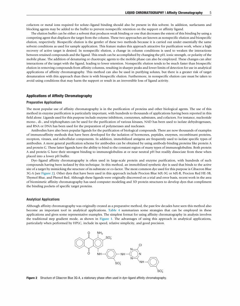
LIQUID CHROMATOGRAPHY | Affinity Chromatography 5
cofactors or metal ions required for solute–ligand binding should also be present in this solvent. In addition, surfactants and
blocking agents may be added to the buffer to prevent nonspecific retention on the support or affinity ligand.
The elution buffer can be either a solvent that produces weak binding or one that decreases the extent of this binding by using a
competing agent that displaces the target from the column. These two approaches are known as nonspecific elution and biospecific
elution, respectively. Biospecific elution is the gentler of these two methods because it is carried out under essentially the same
solvent conditions as used for sample application. This feature makes this approach attractive for purification work, where a high
recovery of active target is desired. In nonspecific elution, a change in column conditions is used to weaken the interactions
between retained compounds and the ligand. This result can be accomplished by changing the pH, ionic strength, or polarity of the
mobile phase. The addition of denaturing or chaotropic agents to the mobile phase can also be employed. These changes can alter
interactions of the target with the ligand, leading to lower retention. Nonspecific elution tends to be much faster than biospecific
elution in removing compounds from affinity columns, resulting in sharper peaks and lower limits of detection for use in analytical
applications of affinity chromatography. This method can also be used in purifying solutes, but there is a greater risk of target
denaturation with this approach than there is with biospecific elution. Furthermore, in nonspecific elution care must be taken to
avoid using conditions that may harm the support or result in an irreversible loss of ligand activity.
Applications of Affinity Chromatography
Preparative Applications
The most popular use of affinity chromatography is in the purification of proteins and other biological agents. The use of this
method in enzyme purification is particularly important, with hundreds to thousands of applications having been reported in this
field alone. Ligands used for this purpose include enzyme inhibitors, coenzymes, substrates, and cofactors. For instance, nucleotide
mono-, di-, and triphosphates can be used for the purification of various kinases, NAD has been used to isolate dehydrogenases,
and RNA or DNA has been used for the preparation of polymerases and nucleases.
Antibodies have also been popular ligands for the purification of biological compounds. There are now thousands of examples
of immunoaffinity methods that have been developed for the isolation of hormones, peptides, enzymes, recombinant proteins,
receptors, viruses, and subcellular components. In addition, immobilized antigens are frequently used to isolate specific types of
antibodies. A more general purification scheme for antibodies can be obtained by using antibody-binding proteins like protein A
and protein G. These latter ligands have the ability to bind to the constant region of many types of immunoglobulins. Both protein
A and protein G have their strongest binding to immunoglobulins at or near neutral pH but readily dissociate from these when
placed into a lower pH buffer.
Dye–ligand affinity chromatography is often used in large-scale protein and enzyme purification, with hundreds of such
compounds having been isolated by this technique. In this method, an immobilized synthetic dye is used that binds to the active
site of a target by mimicking the structure of its substrate or co-factor. The most common dye used for this purpose is Cibacron Blue
3G-A (see Figure 2). Other dyes that have been used in this approach include Procion Blue MX-3G or MX-R, Procion Red HE-3B,
Thymol Blue, and Phenol Red. Although these ligands were originally discovered on a trial and error basis, recent work in the area
of biomimetic affinity chromatography has used computer modeling and 3D protein structures to develop dyes that compliment
the binding pockets of specific target proteins.
Analytical Applications
Although affinity chromatography was originally created as a preparative method, the past few decades have seen this method also
become an important tool in analytical applications. Table 4 summarizes some strategies that can be employed in these
applications and gives some representative examples. The simplest format for using affinity chromatography in analysis involves
the traditional step gradient mode, as shown in Figure 1. The advantages of using this approach in analytical applications,
particularly when performed by HPLC, include its speed, relative simplicity, and good precision.
O
O
NH2
NH NH
NH
SO3
N
NN
CI
–
SO3–
SO3–
Figure 2 Structure of Cibacron Blue 3G-A, a stationary phase often used in dye–ligand affinity chromatography.

Table 4 Analytical applications of affinity chromatographya
General application Examples of analytes
Direct detection Anti-idiotypic antibodies, antithrombin III, bovine growth hormone, fibrinogen, fungal carbohydrate antigens, glucosetetrasaccharide, glutamine synthetase, granulocyte colony stimulating factor, group A-active oligosaccharides, humanserum albumin, immunoglobulin G, immunoglobulin E, interferon, interleukin-2, lymphocyte receptors, b2-microglobulin, tissue-type plasminogen activator, transferrin
Offline affinity extraction Aflatoxin, albuterol, benzodiazepines, cytokinins, fumonisin, human chorionic gonadotropin, ivermectin and avermectin,nortestosterone, ochratoxin A, oxytocin, phenylurea herbicides, sendai virus protein, trenbolone, triazine herbicides
Online affinity extraction Aflatoxin M1, b-agonists, a1-antitrypsin, atrazine, atrazine metabolites, benzylpenicilloyl-peptides, bovine serum albumin,carbendazim, carbofuran, chloramphenicol, clenbuterol, cortisol, dexamethasone, diethylstilbestrol, digoxin, estrogens,hemoglobin, human epidermal growth factor, human growth hormone variants interferon a-2, LSD, lysozyme variants
Chromatographicimmunoassays
Adrenocorticotropic hormone, a-amylase, atrazine/triazines, 2,4-dinitrophenyl lysine, human chorionic gonadotropin,human serum albumin, immunoglobulin G, isoproturon, parathyroid hormone, phenytoin, testosterone, theophylline,thyroid stimulating hormone, thyroxine, transferrin, transferrin, trinitrotoluene
aThe information in this table is based on data provided in Hage (1998).
Sample applicationbuffer Waste
Immunoextractionelution buffer
Immunoextractioncolumn
RPLCsolvent
RPLC analyticalcolumn
Waste
RPLCprecolumn
Figure 3 Scheme for interfacing an immunoextraction column with reversed-phase liquid chromatography (RPLC). The two circles represent six-portswitching valves, with the solid and dashed lines showing the two positions of these values and the flow of sample and solvents in each of the twopositions. The operation of this system is described in the text.
6 LIQUID CHROMATOGRAPHY | Affinity Chromatography
Affinity extraction is another approach that can be used for solute detection. In this method, an affinity column is used for the
removal of a specific solute or group of solutes from a sample prior to their determination by a second method. This approach
employs the same operating scheme as shown in Figure 1 but now involves combining the affinity column either offline or online
with some other method for the actual quantitation of analytes. This scheme often involves the use of antibodies as ligands, but
other binding agents can also be employed.
Offline extraction is the easiest and most common way for combining affinity columns with other analytical techniques. This
method typically involves the use of antibodies that are immobilized and packed into a disposable syringe or solid-phase extraction
cartridge. After conditioning the affinity column with the necessary application buffer or conditioning solvents, the sample is
applied and undesired sample components are washed away. An elution buffer is then passed through the column and the target is
collected. If desired, the collected fraction can be analyzed directly or first dried down and reconstituted in a solvent that is more
compatible with the method to be used for quantitation.
Online affinity extraction can also be used. A typical scheme for performing online immunoextraction with reversed-phase
liquid chromatography (RPLC) is shown in Figure 3. This particular scheme involves injecting the sample onto an immunoextrac-
tion column, with this column later being switched online with a RPLC column. An elution buffer is then applied to dissociate any
retained analyte, which will be captured and reconcentrated at the head of the RPLC column. After all solutes have left the
immunoaffinity column, this column is switched back offline and regenerated by passing through the initial application buffer.
Meanwhile, the RPLC column is developed with either an isocratic or gradient elution scheme that uses a mobile phase with
increased organic modifier content. As the solutes elute through the RPLC column, they are monitored and quantitated through the
use of an online detector.
A third way affinity chromatography has been used in analytical applications is through a chromatographic, or flow-injection,
immunoassay. This method is used in determining trace analytes that do not directly produce a readily detectable signal. The
competitive binding assay is the most common format used in such an assay. This is generally accomplished by mixing the sample

0 6 12 18 24
Time (min)R
esp
onse
(a)
(b)
Figure 4 Detection of a parathyrin in human plasma by a chromatographic-based sandwich immunoassay. The results in (a) show the injectionspikes and nonretained fractions for four sequential injections of human plasma samples with increasing parathyrin levels. The results in (b) show theresponse due to the retained parathyrin. This plot was obtained from Hage, D.S.; Kao, P.C., Anal. Chem. 1991, 63, 586–595.
0 5 10 15
Time (min)
Res
pon
se
[Phenytoin] L–Tryptophan
40 µmol l−1
30 µmol l−1
20 µmol l−1
10 µmol l−1
0 µmol l−1
Figure 5 An example of a zonal elution experiment, in which small injections of L-tryptophan are made onto an immobilized human serum albumincolumn in the presence of increasing amounts of phenytoin in the mobile phase.
LIQUID CHROMATOGRAPHY | Affinity Chromatography 7
with a fixed amount of a labeled analyte analog (i.e., the ‘label’) and simultaneously or sequentially injecting these onto an
immunoaffinity column that contains a limiting amount of antibody. Immunometric assays have also been performed on
chromatographic systems. For instance, in a sandwich immunoassay (i.e., a two-site immunometric assay), two different types
of antibodies are used (see Figure 4). The first of these two antibodies is attached to a solid-phase support and used to extract the
analyte from samples. The second antibody contains an easily measured tag and serves to place a label on the analyte, thus allowing
it to be quantitated.
Biophysical Applications
Besides its use in separating and quantitating sample components, affinity chromatography can also be employed as a tool for
studying solute–ligand interactions. This approach is called analytical, or quantitative, affinity chromatography. Using this
technique, information can be obtained regarding the equilibrium and rate constants for biological interactions, as well as the
number and types of sites involved in these interactions.
Information on the equilibrium constants for a solute–ligand system can be acquired by using the methods of zonal elution or
frontal analysis. Zonal elution involves the injection of a small amount of solute onto an affinity column in the presence of a mobile
phase that contains a known concentration of competing agent. The equilibrium constants for the ligand with the solute (and
competing agent) can then be obtained by examining how the solute’s retention changes as the competing agent’s concentration is
varied (see Figure 5). This method has been used to examine a number of biological systems, such as enzyme-inhibitor binding,

8 LIQUID CHROMATOGRAPHY | Affinity Chromatography
protein–protein interactions, and drug–protein binding. Frontal analysis is used in a similar manner but is performed by continu-
ously applying a known concentration of solute to the affinity column. The moles of analyte required to reach the mean point of the
resulting breakthrough curve is then measured and used to determine the equilibrium constants and number of binding sites for
solute–ligand binding.
Information on the kinetics of solute–ligand interactions can also be obtained using affinity chromatography. A number of
methods have been developed for this, including techniques based on band-broadening measurements, peak fitting, the split-peak
effect, and peak decay analysis. These methods are generally more difficult to perform than equilibrium constant measurements but
represent a powerful means for examining the rates of biological interactions. Systems studied by these techniques have included
the binding of lectins with sugars, protein A, or protein G with immunoglobulins, antibodies with antigens, and drugs with serum
proteins. The recent creation of commercial sensors for biointeraction studies is one result of such work.
Further Reading
1. Allenmark, S. Chromatographic Enantioseparation: Methods and Applications, 2nd ed.; Ellis Horwood: New York, 1991.2. Axen, R.; Porath, J.; Ernback, S. Nature 1967, 214, 1302–1304.3. Chaga, G. S. J. Biochem. Biophys. Methods 2001, 49, 313–334.4. Chaiken, I. M., Ed.; In Analytical Affinity Chromatography; Boca Raton: CRC Press, 1987.5. Cuatrecasas, P.; Wilchek, M.; Anfinsen, C. B. Proc. Natl. Acad. Sci. U.S.A. 1968, 61, 636–643.6. Dean, P. D. G.; Johnson, W. S.; Middle, F. A. Affinity Chromatography – A Practical Approach. IRL Press: Oxford, 1985.7. Hage, D. S.; Kao, P. C. Anal. Chem. 1991, 63, 586–595.8. Hage, D. S. J. Chromatogr. B 1998, 715, 3–28.9. Hage, D. S., Ed.; Handbook of Affinity Chromatography; Boca Raton: CRC Press, 2006.10. Hage, D. S.; Nelson, M. A. Anal. Chem. 2001, 73, 198A–205A.11. Hermanson, G. T.; Mallia, A. K.; Smith, P. K. Immobilized Affinity Ligand Techniques. Academic Press: San Diego, 1992.12. Hjerten, S. Biochim. Biophys. Acta 1964, 79, 393–398.13. Mrabet, N. T.; Vijayalakshmi, M. A. In: Biochromatography-Theory and Practice; Vijayalakshmi, M. A., Ed.; Taylor and Francis: London, 2002; pp 272–294.14. Scouten, W. H. Affinity Chromatography – Bioselective Adsorption on Inert Matrices. Wiley: New York, 1981.15. Starkenstein, E. Biochem. Z. 1910, 24, 210–218.16. Yoo, M. J.; Hage, D. S. In: Monolithic Chromatography and Its Modern Applications; Wang, P., Ed.; ILM Publications: St Albans, 2010, Chapter 1.

Knowledge to Fill in the Gaps.
To start, it helps to know which gaps to fill. Because Elsevier Science and Technology Books has unique visibility into the world’s research output, we share insights that keep you a step ahead. And a step closer to your goal.
BE IN THE KNOW: elsevier.com/sciencedirect/books

3.05 Microarrays
D Amaratunga, Johnson & Johnson Pharmaceutical Research & Development LLC, Raritan,NJ, USA
H Gohlmann and P J Peeters, Johnson & Johnson Pharmaceutical Research & Development,
Beerse, Belgium
& 2007 Elsevier Ltd. All Rights Reserved.
3.05.1 Introduction
873.05.2 Deoxyribonucleic Acid Microarray Experiments
883.05.2.1 Microarray Technologies
883.05.2.2 Experimental Design Considerations
903.05.3 Data Analysis Considerations
913.05.3.1 Data Preprocessing
913.05.3.2 Visual Inspection of the Data
913.05.3.3 Identifying and Studying Differentially Expressing Genes
923.05.3.4 Sample Classification
933.05.4 Case Studies
933.05.4.1 Case Study 1
933.05.4.2 Case Study 2
973.05.4.3 Case Study 3
1003.05.4.4 Conclusions from the Case Studies
1033.05.5 Discussion and a Look to the Future
103References
1043.05.1 Introduction
For the pharmaceutical industry, undoubtedly the most enticing prospect stemming from the modern genomics
revolution is the promise it offers of improved drug target identification. A drug target is a molecule in the body, usually
a protein, that is intrinsically associated with a particular disease process and that could be addressed by a drug to
produce a desired therapeutic effect. Typical examples for such targets are receptors on the surface of a cell that can be
triggered to give a signal upon stimulation with a drug or enzymes whose activity of converting one substance to
another is modulated via a drug. The identification, characterization, and validation of a drug target is a long and
difficult exercise, demanding, as it does, a profound understanding of a disease’s etiology and the biological processes
associated with it, coupled with a fair amount of trial and error experimentation. In fact, up to now, drugs have been
developed to address only a few hundred known drug targets. On the other hand, the anticipation is that today’s
research in genomics and proteomics will yield several thousand new drug targets.
Furthermore, it is likely that these drug targets will lead to drugs that are therapeutically more precise and more
effective than those available today. Many of today’s drugs were identified by happenstance and show a multitude of side
effects. While some lack of specificity may be desirable in certain circumstances, it is still preferable to have substances
that are as specific toward their respective targets as possible to avoid undesirable adverse events. Using our ever-
increasing understanding of how proteins react and interact with each other, it is expected that, for a given disease, the
best possible molecular intervention point should be precisely identifiable. In order to get there, there is a need for
experimental procedures that will capture the behavior of all involved interaction partners simultaneously. Such
procedures are currently emerging in the genomics area with technologies such as deoxyribonucleic acid (DNA)
microarrays for gene activity (¼mRNA) profiling, and in related areas such as proteomics, metabolomics, and lipidomics.
The advent of DNA microarrays was heralded by the seminal paper of Schena et al.,1 who introduced the concept of
immobilizing microscopic amounts of DNA fragments on glass substrates, and the subsequent success story of Golub
et al.,2 who demonstrated that such microarrays could be used both to distinguish among clinically similar types of
87

88 Microarrays
cancer, acute myeloid leukemia, and acute lymphoblastic leukemia, as well as to generate a list of genes associated with
the classification.
The power of DNA microarray technology is that it provides a high throughput instrument for simultaneously
screening thousands of genes for differential expression across a series of different conditions. Despite the fact that it
may not have sufficient sensitivity to detect subtle expression changes such as those of regulatory genes, a well-
designed and properly executed microarray experiment should be able to detect the downstream effects of such
changes, which generally tend to be more dramatic. Since these effects are the ones most likely to be associated with
druggable targets, DNA microarrays are an important tool for identifying drug targets.
The remainder of this chapter is organized as follows. Section 3.05.2 outlines DNA microarray technology and
experiments. Section 3.05.3 describes the various data analysis considerations that are necessary to make sense out of
the enormous datasets generated by these experiments. Section 3.05.4 presents a series of case studies from the
neuroscience area, although the concepts illustrated therein apply much more globally. Finally, Section 3.05.5 offers
some concluding remarks as well as a quick look to the future.
3.05.2 Deoxyribonucleic Acid Microarray Experiments
DNA microarray technology enables scientists to simultaneously assess the relative transcription levels of several (if not
all) of the genes within a cell across a series of different conditions: for example, across different pathological
conditions, such as healthy versus diseased, different disease states, across time during the progression of a disease or
infection, or during therapy and so on. Under the premise that some genes would be differentially expressed as a
consequence of a disease process, monitoring expression patterns in this way provides scientists with potentially
valuable clues and insights for scrutinizing and understanding the biological and cellular processes underlying that
disease.
DNA microarrays are small solid supports (such as glass microscope slides, silicon chips, beads, or nylon membranes)
onto which nucleic acid sequences (probes) have been robotically attached in a rectangular array format. Typically, the
number of probes arrayed is very large and would correspond to a significant representation of the genome under study,
which is in keeping with the concept that this technology is essentially a high throughput screen of the transcriptome.
The probes are usually made of small single-stranded DNA sequences (either oligonucleotides or denatured
polymerase chain reaction (PCR) products), which are expected to be exactly matching (complementary) to the single-
stranded fluorescently labeled target that is finally applied to the microarray. The selection of such short probes is
driven by the annotation of the genome of a given organism. The information at the start and the end of a gene plus the
untranslated regions of the corresponding mRNA is of high importance for the actual selection of the probe sequence.
Owing to the working mechanism of one key enzyme (the reverse transcriptase), the probe sequences tend to be
preferentially selected from the 30-end or the untranslated region of the mRNA.
The labeled target is prepared from mRNA extracted from a biological sample. The mRNA is reverse transcribed
using oligo dT as primer, linearly amplified, fluorescently labeled by incorporating Cy5- or Cy3-deoxynucleotides or
biotinylated deoxynucleotides to which fluorochromes can attach, solubilized in hybridization buffer, and then
dispersed over the surface of the microarray. The microarray slide is then inserted into a sealed hybridization chamber
to allow hybridizations between corresponding sequences on the microarray (i.e., the probes) and in the sample (i.e.,
the labeled target) to occur. Following incubation, the slide is washed using stringent and nonstringent buffers to
remove excess sample from the array and to reduce cross-hybridization. The occurrences of any true hybridization for
any of the probes are indicated by the remaining fluorescent intensities as measured by a confocal laser microscope or
similar instrument. Figure 1 shows schematically the key steps involved in a typical microarray experiment.
A standard microarray experiment would comprise several samples run through the above process. Comparing the
resulting fluorescent intensities across the different samples would indicate which genes are differentially expressed
across them.
3.05.2.1 Microarray Technologies
Several different microarray technologies are commercially available from a number of suppliers, such as Affymetrix and
GE Healthcare, or they may be produced by an in-house laboratory. A few of the more common microarray technologies
are described below.
In a cDNA microarray, the probes are long DNA fragments (a few hundred bases to several kilobases in length) with
sequences complementary to the sequences of the genes of interest or representative subsequences thereof.1 Regions
of low complexity are usually excluded as they could diminish hybridization specificity. cDNA probes can be obtained
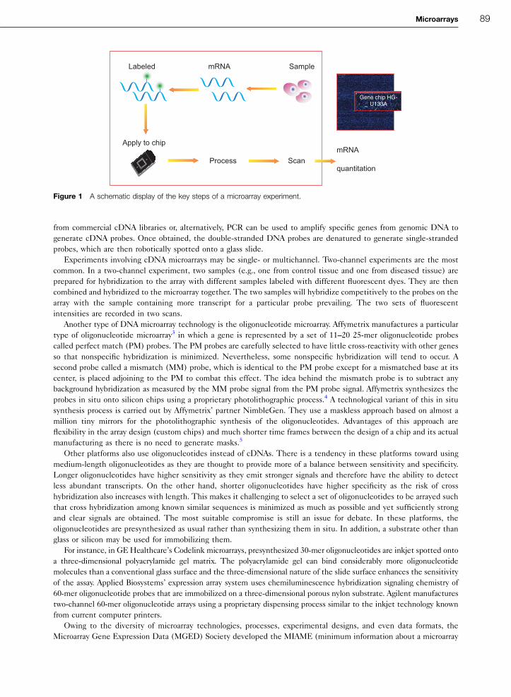
mRNA
quantitation
mRNALabeled
Scan
Sample
Apply to chip
Process
Gene chip HG-U133A
Figure 1 A schematic display of the key steps of a microarray experiment.
Microarrays 89
from commercial cDNA libraries or, alternatively, PCR can be used to amplify specific genes from genomic DNA to
generate cDNA probes. Once obtained, the double-stranded DNA probes are denatured to generate single-stranded
probes, which are then robotically spotted onto a glass slide.
Experiments involving cDNA microarrays may be single- or multichannel. Two-channel experiments are the most
common. In a two-channel experiment, two samples (e.g., one from control tissue and one from diseased tissue) are
prepared for hybridization to the array with different samples labeled with different fluorescent dyes. They are then
combined and hybridized to the microarray together. The two samples will hybridize competitively to the probes on the
array with the sample containing more transcript for a particular probe prevailing. The two sets of fluorescent
intensities are recorded in two scans.
Another type of DNA microarray technology is the oligonucleotide microarray. Affymetrix manufactures a particular
type of oligonucleotide microarray3 in which a gene is represented by a set of 11–20 25-mer oligonucleotide probes
called perfect match (PM) probes. The PM probes are carefully selected to have little cross-reactivity with other genes
so that nonspecific hybridization is minimized. Nevertheless, some nonspecific hybridization will tend to occur. A
second probe called a mismatch (MM) probe, which is identical to the PM probe except for a mismatched base at its
center, is placed adjoining to the PM to combat this effect. The idea behind the mismatch probe is to subtract any
background hybridization as measured by the MM probe signal from the PM probe signal. Affymetrix synthesizes the
probes in situ onto silicon chips using a proprietary photolithographic process.4 A technological variant of this in situ
synthesis process is carried out by Affymetrix’ partner NimbleGen. They use a maskless approach based on almost a
million tiny mirrors for the photolithographic synthesis of the oligonucleotides. Advantages of this approach are
flexibility in the array design (custom chips) and much shorter time frames between the design of a chip and its actual
manufacturing as there is no need to generate masks.5
Other platforms also use oligonucleotides instead of cDNAs. There is a tendency in these platforms toward using
medium-length oligonucleotides as they are thought to provide more of a balance between sensitivity and specificity.
Longer oligonucleotides have higher sensitivity as they emit stronger signals and therefore have the ability to detect
less abundant transcripts. On the other hand, shorter oligonucleotides have higher specificity as the risk of cross
hybridization also increases with length. This makes it challenging to select a set of oligonucleotides to be arrayed such
that cross hybridization among known similar sequences is minimized as much as possible and yet sufficiently strong
and clear signals are obtained. The most suitable compromise is still an issue for debate. In these platforms, the
oligonucleotides are presynthesized as usual rather than synthesizing them in situ. In addition, a substrate other than
glass or silicon may be used for immobilizing them.
For instance, in GE Healthcare’s Codelink microarrays, presynthesized 30-mer oligonucleotides are inkjet spotted onto
a three-dimensional polyacrylamide gel matrix. The polyacrylamide gel can bind considerably more oligonucleotide
molecules than a conventional glass surface and the three-dimensional nature of the slide surface enhances the sensitivity
of the assay. Applied Biosystems’ expression array system uses chemiluminescence hybridization signaling chemistry of
60-mer oligonucleotide probes that are immobilized on a three-dimensional porous nylon substrate. Agilent manufactures
two-channel 60-mer oligonucleotide arrays using a proprietary dispensing process similar to the inkjet technology known
from current computer printers.
Owing to the diversity of microarray technologies, processes, experimental designs, and even data formats, the
Microarray Gene Expression Data (MGED) Society developed the MIAME (minimum information about a microarray

90 Microarrays
experiment) guidelines as a standardized platform for storing and annotating microarray data with a view toward
encouraging the generation, storage, and exhange of microarray data in a controlled manner.3
Each microarray platform has its own advantages and disadvantages.6 The greater length of the probes arrayed on
cDNA microarrays ensures that they hybridize to sample sequences with higher stringency and are less likely to be
affected by minor mutations, but they exhibit lower hybridization sensitivity as longer sequences have higher likelihood
for nonspecific binding. They are less expensive to produce than commercial off-the-shelf arrays when produced in
quantity and thereby offer some flexibility along with the ability to be customized if manufactured in-house. Then
again, they tend to demand much more time and labor-intensive effort in manufacturing, clone maintenance, PCR
work, and quality control. On the other hand, commercial oligonucleotide microarrays tend to yield more reproducible
results that often also show higher specificity.7 The disadvantage of using such platforms is certainly the price, and
often there are organizational problems caused by having to rely on central facilities. Owing to the necessity of utilizing
comparably expensive specialized equipment, many research institutions have had to set up core teams dedicated to
performing the microarray work. Regrettably, this removes part of the control a researcher has over his whole
experiment.
Other applications of DNA microarrays in drug target research have recently gained more attention but will not be
addressed in this chapter further as they require their own experimental design and analysis techniques. Some of these
new applications are comparative genomic hybridization (CGH)8 for the detection of deletions and/or amplifications of
longer DNA stretches in the genome, resequencing of specific DNA sequences in a high throughput fashion, and single
nucleotide polymorphism (SNP) analysis9 for the study of inter-individual differences in single nucleotides within the
genome, to name a few.
3.05.2.2 Experimental Design Considerations
It is imperative to design a microarray experiment so that its objectives can be met. The objective of many microarray
experiments is to identify which genes are differentially expressed among several sets of samples. In such comparative
experiments, it is important to be able to generate statistics about what could be considered a differentially expressed
gene. This means that replicate samples must be run in order to generate enough data for a statistical analysis to have
adequate power to detect gene expression changes. As microarray experiments tend to be expensive, researchers are
sometimes reluctant to do too many replicates. However, both natural biological variability and the series of highly
technical steps that constitutes a microarray experiment cause the data to be subject to various sources of variation.
Minor differences in extraction, amplification, labeling, hybridization, and even the skill and experience of the
experimenter could result in substantial differences among what would otherwise be true replicates.
Only with sufficient replication can this variability be overcome and statistical significance assessed adequately.
There are two types of replication. One type is ‘biological replication,’ which involves extracting mRNA from several
biological samples and running each sample on a different microarray in order to compensate for intrinsic biological
variability in gene expression. The other type is ‘technical replication,’ which involves running the same sample on
multiple arrays in order to compensate for the technical variability of the experimental process.
Sometimes an experiment might turn out to be too large or too complex to be completed in a single session. In that
case, it is important to allocate, organize, and run the arrays in such a way that the effects of interest are not
confounded with extraneous effects, such as operator effects, manufacturing batch effects, and hybridization day
effects.
In general, it is crucial to pay careful attention to quality issues in order to ensure validity of the conclusions reached
from the study. The mRNA source and the preparation of the samples should be controlled and their quality assessed.
The most common techniques used nowadays are classical agarose gel electrophoresis to assess potential mRNA
degradation, spectrophotometrical analysis using a very small quantity of total RNA in a Nanodrop, and miniaturized
electrophoresis technologies such as the Agilent Bioanalyzer, which can produce data on mRNA degradation as well as
mRNA quantity. The whole issue of mRNA quality is largely dependent on the source from which the mRNA is
prepared. Cells cultivated in in vitro cultures tend to be much more homogeneous and generally yield much more
consistent mRNA quality and quantity as compared to mRNA from tissues. Furthermore, it is much easier to extract
mRNA from some tissues than others: While it is fairly easy to extract mRNA from liver, tissues such as heart or spleen
require much more experience to obtain the high-quality mRNA necessary for microarray analysis.
In addition, several control probes are often arrayed on the microarrays for various quality control purposes. The
most common are negative control probes, which are used to assess background and nonspecific hybridization, and
positive control probes, which are used to measure the abundance of nucleic acid sequences spiked in to the labeled
target as a way of assessing labeling and hybridization efficiencies.

Microarrays 91
3.05.3 Data Analysis Considerations
Owing to the volume and complexity of the data generated by DNA microarray experiments, the data analysis aspect of
these studies acquires greater importance than other areas of biomedical research. In order to derive substantive
biological information from these studies, careful experimental design and proper statistical and bioinformatics analysis
are vital. Typically, a data analysis would consist of several stages. The first stage is always a data preprocessing step,
which will be described next. The subsequent stages depend on the objective of the experiment.
3.05.3.1 Data Preprocessing
Preprocessing the raw intensity data enhances the sensitivity of the downstream comparisons. Some preprocessing
steps, in the sequence in which they would normally be performed, are:
1. Array quality check: While a certain amount of variation in the intensity values across even identical arrays is
inevitable and not a cause for concern, it is not uncommon, given the technical complexity of the experimental
process, that a few arrays or a few samples in a study turn out to be defective. It is essential, however, to detect and
eliminate them so that they do not unduly affect the data analysis. Arrays or groups of arrays that are substantially
different from the rest can be identified by calculating Spearman correlation coefficients between all pairs of arrays.
The resulting correlation matrix can be displayed on a heatmap by coloring each correlation on the basis of its value.
This will highlight any unusual arrays, samples of poor quality, and bad hybridizations, which will generally tend to
have low correlations with most, if not all, of the other arrays and will therefore stand out in the plot.
2. Data re-expression: Microarray data are generally very heavily skewed. Furthermore, the distribution of the intensity
values could be quite different for different genes, most noticeably between low-expressing genes and high-
expressing genes. The within-gene distribution can be symmetrized and the heterogeneity of variances across the
genes greatly reduced by transforming the data. More often than not this can be achieved via a simple logarithmic
transformation (logarithms of base 2 are often used). However, sometimes, some other transformation, such as a
variance stabilizing transformation, a hybrid linear log transformation, or a started log transformation will do better.
3. Normalization: Spot intensity data will often need to be normalized to reduce monotonic nonlinear array effects.
Care must be taken when doing so to ensure that gene-specific effects are at most only slightly dampened,
otherwise detecting differential expressed genes will become impossible. Quantile normalization is a popular
normalization procedure. A reference array, to which all the arrays are normalized, is defined, usually as an average
microarray, such as by calculating gene-wise either the mean or the median across all the arrays. The distributions of
the transformed spot intensities are coerced to be as similar as possible to that of the transformed spot intensities of
the reference array. Quantile normalization is useful for normalizing a series of arrays where it is believed that a small
but indeterminate number of genes may be differentially expressed across the arrays, yet it can be assumed that the
distribution of spot intensities does not vary substantially from array to array. This assumption is often valid, and
when it is not, the normalization would have to be customized to the particular data being analyzed.
4. Final quality checks: Inevitably, the data will contain a few unusual spot intensity values (i.e., outliers). By
identifying and either removing or downweighting such aberrant values, the adverse impact that they would
otherwise have on subsequent analyses can be reduced. This can be done by comparing replicates, which can be
expected to be very similar to one another. In addition, a final array check can be done via a principal component
analysis (PCA) or spectral map analysis as described in (see Section 3.05.4.2).
Details of these preprocessing steps and others are described in 10.
3.05.3.2 Visual Inspection of the Data
Gene expression data is typically organized into a gene expression matrix in which the columns represent the samples
or experiments and the rows represent the expression vectors for the genes being interrogated by the microarray. The
matrix elements are either the spot intensities preprocessed as above or fold changes based on the spot intensities. In
trying to expose patterns in this data, it is helpful to somehow render this matrix visually.
A commonly used simple approach is to display the gene expression matrix as a heatmap by coloring each matrix
element on the basis of its value. It is likely that the heatmap will initially appear to be devoid of any apparent pattern
or order. However, by reordering the rows and/or columns on the basis of a clustering of the genes and/or samples,
potentially interpretable patterns of gene expression will often emerge, as groups of co-regulated genes should occupy
adjacent or nearby rows and similar samples should occupy adjacent or nearby columns in the display.

92 Microarrays
PCA is another method for visually presenting the data with a view toward revealing structures in the gene
expression vectors. PCA is a technique for summarizing a multidimensional dataset in a few dimensions. Noting that
the gene expression matrix has as many dimensions as it has genes, some serious dimension reduction is necessary
without too much reduction in information in order for this to produce a meaningful representation. Methodologically,
PCA finds a new coordinate system such that the first coordinate, a linear combination of the columns of the data
matrix, has maximal variance, the second coordinate has maximal variance subject to being orthogonal to the first, and
so on. Plotting the first few coordinates often reveals interesting patterns. For instance, samples sharing similar profiles
will tend to lie close to each other. A rough visual estimation of the number of clusters represented in the data should
also be possible. In addition, PCA may reveal oddities in the data, such as unusual arrays, and it therefore provides a
useful supplementary array quality check as stated in (see Section 3.05.3.1).
A number of methods similar to PCA have been developed and project different views of the data. Factor analysis,
correspondence factor analysis, multidimensional scaling, and projection pursuit are some of the better known ones.
The biplot and spectral map analysis are extensions of these ideas. The PCA described above is PCA applied to the
samples (i.e., to the columns of the gene expression matrix). PCA can also be applied to the genes (i.e., to the rows of
the gene expression matrix). When a form of PCA, called the singular value decomposition, is applied to both samples
and genes, the simultaneous representation of both samples and genes in a single plot is called a biplot. Thus, a biplot
will consist of both sample-related points and gene-related points. As in a PCA plot, the distances between the sample-
related points are related to the dissimilarities between the samples; the closer a set of sample-related points, the more
similar the samples to which they correspond. Most gene-related points will clump together in the center of the biplot;
these would correspond to genes that are not differentially expressing across the samples. Any gene-related points that
lie substantially away from this central clump in the direction of a cluster of sample-related points would correspond to
genes whose expression profiles are associated with that cluster of samples. Thus, a biplot could be used to reveal not
only clusters of samples but also the genes associated with them. As a variation, prior to constructing a biplot, the rows
and columns of the gene expression matrix can be centered and weighted in specific ways to allow certain features of
the biplot to be highlighted. This is spectral map analysis.11
3.05.3.3 Identifying and Studying Differentially Expressing Genes
Identifying genes whose changes in expression are most associated with differences between the samples is one of the
fundamental questions addressed in the analysis of gene expression data. Thus, a comparative analysis of the gene
expression levels from a diseased cell versus those of a normal cell will help in the identification of the genes and
perhaps the biological processes and pathways affected by the disease process. Researchers can then use this
information to synthesize drugs that influence and intercede in this process. In order to address this question, both the
magnitude and the consistency of the expression changes must be assessed and a valid and reliable metric of
differential gene expression derived from the preprocessed spot intensity data.
When comparing two sets of samples, the significance of any gene expression change can be assessed by calculating a
t statistic for each gene. The t statistic is essentially a signal-to-noise ratio, in which the difference in mean log spot
intensities (essentially the mean fold change on a log scale) is the signal and the standard error is the noise. Note that
the fold change by itself, although used occasionally, is unreliable because it does not take into account the fact that not
all fold changes can be treated equally which itself is because different genes have different levels of variability. Of
course, the t test must be used carefully too. For instance, when the sample sizes are small, as is common in many
microarray experiments, the value of the t test statistic tends to be overly dependent on the estimate of noise, to
combat which modified versions of the t test (e.g., significance analysis of microarray data-t by 12 and Conditional t
by 10) have been proposed.
When comparing gene expression levels across multiple sets of samples, the t test statistic would be replaced by the
F test statistic. In the event that the experimental situation is more complex, such as a temporal or dose–response
study, appropriate F test statistics associated with linear ANOVA (analysis of variance) models could be used.
Genes that yield statistically significant t (or F) statistics should be examined for corroborating evidence of
biological relevance. Thus, a potentially useful supplementary exercise is to superimpose inter-gene functional
relationships onto the t test (or F test) results.13 Accordingly, a list of genes with statistically significant expression
changes can be examined for the repeated occurrence of various functional annotations, such as gene ontology
classifications, biochemical pathways, or protein–protein interactions. Via a simple statistical analysis, it can be
ascertained whether the set of significant genes contains an over-representation of genes in certain functional
categories. There is at present one obstacle to doing this well and that is the scarcity and the questionable quality of
the annotation data available for genes and their functional interactions. Nevertheless, as annotation databases improve

Microarrays 93
in coverage, quality, and complexity, their integration into microarray results will be more viable and become an
increasingly valuable exercise.
Another potentially useful supplementary exercise is to cluster genes from multiple sets of samples into clusters
with similar expression patterns. Hierarchical and nonhierarchical algorithms such as agglomerative nesting, k-means,
and self-organizing maps have been implemented to cluster similar gene expression patterns. Presuming that genes
performing similar functions or belonging to the same biochemical pathway will exhibit a tendency to co-regulate,
inferences could be made regarding the unknown genes that share a cluster with genes whose functions or pathways are
known. Further inferences can be made by interrogating these clusters as above for over-representation in certain
functional categories.13
3.05.3.4 Sample Classification
When the samples are heterogeneous, they could be clustered using one of the methods listed above. A cluster analysis
will reveal groups of similar samples. If the sample types are known, this exercise can be used as validation that the
experiment was successful at separating the samples. In addition, clustering may indicate the existence of new
subclasses of existing classes of a phenotype or a disease, thereby leading to a better understanding of the situation at
the gene level.
When the samples are known to come from a number of different classes, another primary objective of many DNA
microarray experiments is the classification of the samples into the separate classes. This has two objectives. The first
is to identify the features (in this case, the genes or certain combinations of genes) that are most associated with the
classification. The second is to predict the classification of new samples. Accordingly, classification addresses the
question: given a set of samples, how can one assign each sample into the set of known classes with minimum errors? To
do this, a set of feature variables is defined and a decision rule (i.e., a classifier) based on these feature variables is
derived such that, given the measured values for any sample, the classifier would map it into one of the classes. A
number of methods can be used for classification, including linear discriminant analysis and variants, k nearest
neighbors, random forests, neural networks, and support vector machines. Readers should refer to the References for
examples of various microarray classification methods.10,14
3.05.4 Case Studies
In an ideal situation the identification of novel drug targets in a given disease is performed using diseased and control
tissue. However, biological samples derived from a precisely defined patient population and matched controls are
scarce. An exception to this rule is the field of oncology research, where profiling experiments can be performed on
tumor tissue and healthy control tissue derived from the same patient. In contrast, at the other end of the spectrum,
are the diseases of the central nervous system for which it is much more complicated to obtain affected tissue. As an
alternative, post-mortem samples are mostly used in diseases such as bipolar disorder, major depression, and
schizophrenia. This complication might be resolved in the future if reports on the possible correlation between
expression patterns observed in the brains and lymphoblastoid cells in patients with bipolar disorder, are confirmed.15
As an alternative to patient samples, scientists have turned to animal and cellular models of disease to study changes
in gene expression related to the etiology and progression of disease states. Both animal and cellular systems can also be
used for mode of action studies. In the following case studies, we will address experimental design, microarray
experiments, and data analysis in real-life examples.
3.05.4.1 Case Study 1
The aim of the first case study was to elucidate pathways downstream of the corticotropin-releasing factor (CRF)
receptor CRF1 in order to identify novel modulators of this receptor-signaling pathway.16 CRF is a 41-amino-acid
polypeptide that plays a central role in the regulation of the hypothalamic-pituitary-adrenal (HPA) axis, mediating
neuroendocrine, autonomic, and behavioral responses to various stressors.17 Hypothalamic neurons release CRF in
response to stress, stimulating the secretion of adrenocorticotropic hormone (ACTH) from the pituitary, which in turn
leads to increased release of glucocorticoids from the adrenal glands. Alterations in the CRF system activity have been
linked to a number of psychiatric disorders, including anxiety and depression. Since the pituitary is the main target organ
for CRF, the study was performed on a mouse pituitary-derived cell line called AtT-20 that expresses the CRF1 receptor.
Experimenting on freshly isolated pituitary cells probably would be closer to the in vivo situation compared to the
artificial AtT-20 cell line. However, the pituitary is a heterogeneous organ, comprising many different cell types, of which

94 Microarrays
only a subset (the corticotrophs) respond to CRF. Therefore, changes in gene expression profile in this subset of cells
might be diluted when studying the whole organ. In that sense, not withstanding the fact that AtT-20 cells are derived
from a mouse pituitary cancer, they are considered a good cellular model of corticotrophs. The experimental setup of this
case was as follows: AtT-20 cells were exposed either to CRF, CRF in combination with the CRF1 antagonist R121919,37
antagonist alone, or vehicle (DMSO). The transcriptional response to these four treatments was followed over time
starting from 0 to 24 h after start of the treatment. Thus, in total 25 samples were processed: time 0 and 6 other time
points for each of the four treatments. A downside of this design is the lack of replicates of a specific treatment at each
time point. After processing the RNA samples on Affymetrix microarrays, data were preprocessed as described above. In
this case data were transformed using a logarithmic transformation with base 2. After transformation, data were
normalized using quantile normalization,18 taking into account the fact that Affymetrix arrays have a limited array-to-
array variation. After this preprocessing, data were visually inspected using spectral map analysis. As described above
(see Section 3.05.3.2), this summarizing technique allows similarities between samples to be identified in an unbiased
way based on overall gene expression patterns. In addition, relations between samples and genes can be identified on the
biplot. In this specific case the spectral map allowed the identification of both an effect of progressing time and CRF
exposure on gene expression. As shown in Figure 2, in the biplot of the first two principal components, samples are
clustered clock-wise according to time exposed to a certain treatment, irrespective of the nature of this treatment.
Interestingly, when plotting the first versus the third principal component differences between the treatments are
visualized. This biplot was further applied to identify genes that contribute to the differences between the samples.
Genes that do not contribute to this difference end up in the middle of the plot around the so-called centroid. Genes
that co-cluster with samples at the periphery of the biplot are genes that show a striking upregulation in that sample. In
this manner several genes were found to be strongly upregulated by CRF exposure. The alternative approach that was
followed consisted of analyzing expression measurements in the different treatments relative to those observed in the
corresponding time point in DMSO-treated control samples. Regulated genes were defined as those showing a greater
than two fold change in transcript levels at any one time point. Eighty-eight genes showed a difference in expression
after treatment with CRF compared to treatment with the antagonist. Based upon the time point where the response
was maximal, genes were classified into ‘early responders,’ ‘intermediate responders,’ and ‘late responders.’ Among the
responders were known players in the pathways downstream of the CRF1 such as the transcription factors Nurr1,
Nurr77, and Jun-B, indicating that the setup could confirm previous data obtained by other means. Of interest is the
observation that 50 of the 88 genes that were identified using this arbitrary fold change criterion were also identified in
the unsupervised spectral map analysis demonstrating the power of this graphical visualization tool.
Confirmation of array data is often done using quantitative PCR techniques such as Taqman technology. In this case
study 21 of the most regulated genes were confirmed using quantitative PCR on an ABIPrism 7700 cycler with
commercially available assays from Applied Biosystems. Data obtained in this way on all of the tested genes confirmed
expression profiles previously observed on the array. Overall, the magnitudes of changes observed with microarray
technology were lower than those obtained using quantitative PCR. Ultimately, confirmation needs to be done using a
non-RNA-dependent method. This could be based on the protein or on protein function. An example of this is the use
of RNA interference (RNAi) technology. By knocking down expression of specific genes identified in the array
experiments using RNAi, one could immediately test hypotheses generated by array data analysis.
Figure 2 Spectral map analysis of the microarray data of AtT-20 cells. (a) The first two principal components (PC) of theweighted spectral map analysis applied to the normalized microarray data for all time points and all treatments. On the spectralmap, squares depict different samples whereas circles depict different genes (the size of the circle corresponds to intensity onan Affymetrix array). The distances between squares are related to the dissimilarities between the samples; the closer a set ofsquares, the more similar the samples to which they correspond. Most circles will clump together in the center of the biplotaround the centroid (depicted by a cross); these correspond to genes that are not differentially expressed across the samples.Any circle that lies substantially away from this central clump in the direction of a cluster of squares corresponds to a genewhose expression profile is associated with that cluster of samples. Those genes contributing significantly (measured by theirdistance from the centroid) to difference between samples are annotated with their Affymetrix identifier.36 The first two PCsidentified time as the major discriminator between the samples, distributing the samples clockwise over the plot starting at theT0 time point and ending at the T24 time point. Inserted heat-maps (insets) show representative genes (indicated in bold in biplot)that are maximally induced either after 4 and 8 h or at 0.5, 1, and 24 h, corresponding to their position on the biplot. (b) Biplot offirst and third PCs. The third PC identifies the specific CRF effect on AtT-20 cells over time. (c) Summary views on the first threedimensions of the spectral map, showing how this technique identified time and CRF effects in the microarray dataset. uvc,unitcolumn-variance scaling; RW, row weight; CW, column weight. Closure¼ none; center¼double; norm.¼global; scale¼uvc;RW, mean; CW, constant. (Reproduced from Peeters, P. J.; Gohlmann, H. W.; Van, D. W. I.; Swagemakers, S. M.; Bijnens, L.;Kass, S. U.; Steckler, T. Mol. Pharmacol. 2004, 66, 1083–1092.)

08.CRF+R12191908.R121919
PC1 25%
PC
2 15
%
100050_at
102362_i_at
102397_at
102410_at
103748_at
104588_at
94428_at95632_f_at
96494_at
96803_at
98478_at
98855_r_at
99077_at
T0
0.5.DMSO
01.DMSO
02.DMSO04.DMSO
08.DMSO
24.DMSO
0.5.CRF
01.CRF
02.CRF
04.CRF
08.CRF
24.CRF
0.5.R121919
01.R121919
02.R121919
04.R121919
24.R121919
0.5.CRF+R121919
01.CRF+R121919
02.CRF+R121919
04.CRF+R121919
24.CRF+R121919
DMSO
CRF
R
CRF+R
96494_at0.5 1 2 4 8 24 h
95632_f_at0.5 1 2 4 8 24 h
DMSO
CRF
R
CRF+R
1 3 4 5 6 72 1 3 4 5 62 7
(a)
Mic
roa
rrays
95

T0
0.5.DMSO
01.DMSO02.DMSO
04.DMSO
08.DMSO
24.DMSO0.5.CRF
01.CRF
02.CRF
24.CRF0.5.R121919
01.R121919
02.R121919
08.R121919
0.5.CRF+R121919
01.CRF+R12191902.CRF+R121919
04.CRF+R121919
08.CRF+R121919 24.CRF+R121919
PC1 25%
PC
3 9%
100533_s_at
102362_i_at
102410_at
102907_at
104588_at
104712_at
92205_at
94428_at
95632_f_at
96055_at
96326_at
96494_at
97844_at
04.CRF08.CRF
04.R121919 24.R121919
(b)
Figure 2 Continued
96
Mic
roa
rrays

PC1 25%
PC
3 9%
CRF
CRF & R
T0/DMSO/R
PC1 25%
PC
2 15
%T0DMSOCRFRCRF & R
T0DMSOCRFRCRF & R
0 h
0.5 h
1 h
2 h
4 h
8 h
24 h
(c)
Figure 2 Continued
Microarrays 97
3.05.4.2 Case Study 2
In a second case study profiling experiments were done on transgenic animals rather than cell cultures. The aim of this
study was to elucidate molecular signatures present in different brain regions of transgenic mice overexpressing CRF
(CRF-OE).19 These signatures are hypothesized to underlie homeostatic mechanisms induced by lifelong elevated
CRF levels in the brain. In line with a role of brain CRF in the mediation of endocrine, autonomic, and behavioral
responses to stress, transgenic mice overexpressing CRF (CRF-OE) have been reported to show increased anxiety-
related behavior, cognitive impairments, and an increased HPA axis activity in response to stress.20,21 These animals
therefore are considered to constitute a good animal model for chronic stress and as an extension thereof, depression.
At least part of the behavioral and cognitive changes observed in CRF-OE mice can be attenuated by central
administration of a CRF antagonist.
The experimental design of this study aimed at elucidating differences between CRF-OE animals and their wild-
type littermates in addition to the effects on gene expression profiles of administrating 10 mg kg� 1 of R121919, a CRF1
receptor antagonist. To this end six experimental groups were defined. Half of the groups consisted of CRF-OE
animals, the other half of wild-type littermates. Animals were either untreated, vehicle treated, or compound treated
twice a day for five consecutive days. In experiments using transgenic animals the number of animals is often the
limiting factor, which is certainly the case with CRF-OE mice, since these mice are notoriously difficult to breed. As a
result each experimental group only consisted of three to four age-matched male animals.
Rather than analyzing whole brain samples, dissection of brain was performed in order to get regional expression
data. In total, expression patterns in six regions were studied, including cerebellum, hippocampus, frontal cortex,
temporal area, nucleus accumbens, and pituitary. The importance of performing these dissections in a standardized way
is exemplified in Figure 3. As shown in the spectral map biplot each mouse brain region is characterized by a specific
gene expression pattern. Deviations in removing certain brain areas resulting in more or less contribution of
surrounding tissue will result in an overall increase of the noise. Therefore consistency is required in removing the
tissue (removal of tissue was performed by one operator).
RNA isolated from different animals was processed separately per individual animal and per brain region on
Affymetrix murine U74 arrays. As in the previous case study, genes that were called absent (nonreliable detection) in all
samples according to Affymetrix’s MAS 5.0 software were removed from further analysis. Raw fluorescence intensities
from each array were log2 transformed and data were quantile normalized. Following the group-wise quantile
normalization per treatment and genotype, a second quantile normalization was carried out across the data of all
samples of a given brain area.18
Visual inspection of overall changes in gene expression profile among different treatment groups was done using
spectral map analysis per brain region. This analysis revealed overt differences in gene expression pattern
predominantly at the level of the pituitary and less so at the level of the other brain areas. Prolonged elevated levels of
CRF as present in CRF-OE are expected to induce major changes in the expression profiles in this organ since it is the

PC
2 12
%
PC1 30%
MybKl
--
Ssr3
Rxrg
Camk2aCalcr
E430003D02Rik
Sdc2
---
Spectral map
Frontal cortexHippocampusNucleus accumbensTemporal area
Figure 3 Spectral map analysis of brain regions from mice. The first two components of this spectral map show clustering ofsamples according to the brain region they are derived from. Genes contributing most are depicted by their gene symbol ifapplicable. The gene for the calcitonin receptor (Calcr) is, for example, more expressed in the nucleus accumbens than in otherbrain regions. In contrast, the gene encoding the calcium/calmodulin-dependent protein kinase II-alpha (Camk2a) is moreabundant in the other brain regions than in the nucleus accumbens. uvc, unit column-variance scaling; RW, row weight; CW,column weight. Closure¼none; Center¼double; Norm.¼global; Scale¼ uvc; RW¼mean; CW¼mean.
98 Microarrays
primary target of CRF. On the pituitary data spectral map the CRF-OE and wild-type samples (depicted by squares in
Figure 4) cluster at opposite sites in the biplot. Genes at the periphery of the biplot (contributing significantly to the
differences in expression profiles between samples) included kallikreins (Klk9, Klk13, Klk16, and Klk26), a family of
serine proteases involved in the processing of biologically active peptides. Upregulation of these enzymes might be an
indication for an overactive pituitary. Treatment with the CRF1 antagonist R121919 or treatment with vehicle did not
induce gross changes in expression profile and did not normalize expression patterns in CRF-OE relative to those
observed in wild-type animals, as illustrated by the spectral map. An underpowered study as a result of the limited
number of animals in each group might account for this negative result. Another more likely explanation is that whereas
changes in behavior of CRF-OE mice are the immediate consequence of CRF1 antagonism, the changes in gene
expression are the consequence of prolonged HPA axis activation that are not easily overcome by treatment for 5 days
with the CRF1 antagonist R121919 as in the above experimental setup. A prolonged treatment and/or a larger group of
animals might overcome these issues, once again stressing the importance of good experimental design.
Since spectral map analysis only revealed differences between transgenic animals and their wild-type littermates,
post hoc analysis was performed on untreated CRF-OE and their corresponding wild-type littermates. Given the low
number of animals per group the significance analysis of microarray data algorithm12 was chosen as an adapted t test for
multiple observations. Significance analysis of microarray data assigns a score to each gene on the basis of change in
gene expression relative to the standard deviation of repeated measurements. For genes with scores greater than an
adjustable threshold, significance analysis of microarray data uses permutations of the repeated measurements to
estimate the percentage of genes identified by chance, i.e., the false discovery rate (FDR).22 Thus, the FDR is the
expected proportion of false positives among the tests found to be significant. An extension of this FDR is the so-called
q-value.16 This q-value is similar to the well-known p-value. It gives each hypothesis test a measure of significance in
terms of a certain error rate. The p-value of a test measures the minimum false-positive rate that is incurred when
calling that test significant. Likewise, the q-value of a test measures the minimum false discovery rate that is incurred

PC
2 10
%
PC1 28%
Spectral map
WT.UWT.VeWT.RCRF-OE.UCRF-OE.VeCRF-OE.R
Klk26
Viaat
Lzp-s
Sult1a1
Ptger4Ceacam 10
Krt1-19
Mmp7
Penk1 Ccl17
Figure 4 Spectral map analysis of pituitary-derived gene expression profiles of CRF overexpressing mice (CRF-OE) comparedto wild-type (WT) mice. Spectral map analysis of microarray data obtained in the pituitary showing the projection of both genesand samples in two dimensions. Positioning of the samples derived from CRF-OE on the opposite side of the centroidcompared to the WT samples along the x-axis (PC1) indicates that 28% of the variation in gene expression levels is explained bythe genotype of the animals. Genes that contribute largely to the difference between WT and CRF-OE (indicated by theirpositioning at the extremities of the graph) are highlighted and depicted by their gene symbol. uvc, unit column-variance scaling;RW, row weight; CW, column weight. Closure¼none; Center¼double; Norm.¼global; Scale¼uvc; RW¼mean; CW¼mean.
Microarrays 99
when calling that test significant. Whereas the p-value is commonly used for performing a single significance test, the
q-value is useful for assigning a measure of significance to each of many tests performed simultaneously, as in microarray
experiments. A 10% threshold is accepted practice for array data analysis (as applied for pituitary data). However,
deviation of this rule of thumb can be made when the number of significantly changed genes is limited. Therefore, a
q-value below 20% was used in all other datasets.
In agreement with the spectral map, only a limited number of genes were significantly altered in most brain areas
with only 10 genes being downregulated in the hippocampus. In the nucleus accumbens 50 genes were downregulated
whereas 11 genes were upregulated. Recurring changes in expression patterns in several brain areas could be clustered
into a few pathways such as the glucocorticoid signaling pathway (exemplified by downregulation of 11b-hydroxysteroid
dehydrogenase type 1 and upregulation of the immunophilin Fkbp5). Adaptations in the glucocorticoid pathway fit
nicely with the CRF changes in CRF signaling, since continued production of CRF in the CRF-OE animals will lead to
an excess of glucocorticoids. This excess of glucocorticoids is counteracted by changing the levels of important players
in that pathway such as 11b-hydroxysteroid dehydrogenase type 1 and Fkbp5. These changes in individual gene
expression profiles in different brain areas could be confirmed by quantitative PCR.
In agreement with results of the spectral map analysis, at the level of the pituitary many more genes (114 genes)
differed significantly in their expression between untreated wild-type and CRF-OE animals and were more than two
times up- or downregulated. When comparing wild-type to CRF-OE animals, 102 genes had a q-value below 10% and
were more than 1.5-fold downregulated in CRF-OE. Similarly, 180 genes had a q-value below 10% and were more than
1.5-fold upregulated in CRF-OE. In agreement with the spectral map, significance analysis of microarray data identified
kallikrein genes Klk9, Klk13, Klk16, and Klk26, but in addition also identified Klk5 and Klk8 to be significantly
upregulated in CRF-OE.
100 Microarrays
A recurring theme revealed by microarray analysis was the downregulation of neurotensin receptor 2 (Ntsr2) mRNA
levels in several brain regions including the hippocampus (� 54%), the nucleus accumbens (� 38%), and the frontal
cortex (� 59%), but not in the pituitary. Although levels of Ntsr1 mRNA were below the detection limit in microarray
analysis, the observation of Ntsr2 mRNA downregulation prompted investigators to study the expression levels of all
members of the neurotensin (NT) receptor family by quantitative PCR. Ntsr3 mRNA did not show any change in
expression in any area tested. Ntsr1 mRNA was significantly downregulated in CRF-OE, with the most pronounced
effect in the hippocampus. Quantitative PCR also demonstrated a 67% downregulation of Ntsr2 mRNA in the
hippocampus, confirming the microarray data. In order to evaluate the changes in Ntsr1 and Ntsr2 mRNA at the
protein level, the presence of receptor (Ntsr1 to Ntsr3) was assessed by autoradiography of [125I]NT binding on brain
sections. In agreement with array and quantitative PCR results, autoradiography data demonstrated an overall (Ntsr1 to
Ntsr3), genetically determined downregulation of the [125I]NT binding capacity in CRF-OE versus wild-type animals.
Blocking of the Ntsr2 receptors by a saturating concentration of levocabastine, unmasked prominent differences in
expression of Ntsr1. A pronounced downregulation of the [125I]NT binding in the CRF-OE animals was observed in
specific brain regions such as the stratum radiatum (� 63.876.5%, p o0.001), the retroslenial granular cortex
(� 49.477.5%), and the temporal cortex (� 34.873.5%). Also, the autoradiography data demonstrated no effect of
subchronic administration of R121919 as seen in the gene expression profiling data. These data clearly demonstrate the
utility of non-RNA-based technologies such as radioligand binding studies to further validate and investigate microarray
data. In addition to the confirmation of quantitative information provided by microarray and PCR this radioligand
binding technique supplies further spatial information on where in the brain changes have occurred.
3.05.4.3 Case Study 3
This final case study deals with the complexity of an animal model for irritable bowel syndrome (IBS) in combination
with the fact that changes in gene expression are believed only to occur in a small subset of cells. The aim of this study
was to investigate long-term changes in gene expression in viscera-specific neurons of both nodose ganglia (NG) and
dorsal root ganglia (DRG) in a postinfectious mouse model of IBS.23 The pathogenesis of IBS is heterogeneous, but at
least in a subpopulation of patients emotional stress and enteric infection have been implicated.24 Therefore, the
mouse model of IBS that was chosen for this study consisted of a transient inflammation induced by the nematode
Nippostrongylus brasiliensis (Nb) combined with exposure to stress. Gene expression profiles were measured both in NG
and DRG visceral sensory neurons because the gastrointestinal tract receives dual extrinsic sensory innervation. Vagal
afferents have their cell bodies in the NG and project centrally to make synaptic connections in the brainstem, mainly
at the level of the nucleus tractus solitarius while spinal afferents arise from the DRG and project into the dorsal horn
of the spinal cord (Figure 5).25 Currently, there is a common view that vagal and spinal afferents have different
functional roles: spinal afferents play a major role in nociception, while vagal afferents mediate physiological responses
and behavioral regulation, particularly in relation to food intake, satiety, anorexia, and emesis. However, there is some
overlap, and vagal and spinal afferents share a number of features in common. Both NG and DRG neurons have been
shown to become sensitized following inflammatory insult, demonstrating plasticity in the mechanisms that regulate
neuronal excitability, which has implications for pain processing.
In this way, extrinsic afferent neurons supplying the gut are prime targets for new treatments of chronic visceral pain
disorders such as IBS. However, fiber-tracing experiments measuring the extent to which abdominal viscera-projecting
neurons23 contribute to the total pool of sensory neurons in the DRG and NG, showed that only 3% are visceral sensory
neurons. This gives an estimate of the extent to which changes in gene expression occurring in this subpopulation is
likely to be diluted when whole ganglia expression is assessed. To circumvent these issues, viscera-specific sensory
neurons were labeled using retrograde labeling with fluorescently tagged cholera toxin beta subunit. Labeled neurons
in DRG (T10 to T13) and NG were isolated using laser-capture microdissection. This laser-captured material was
linearly amplified using a three-round amplification and labeling protocol. To check for linearity of amplification, laser-
captured material was spiked with four poly-adenylated prokaryotic genes at a fixed ratio. For these genes probes are
present on Affymetrix’s microarrays, allowing the efficiency and linearity of the amplification procedure to be
monitored.
As mentioned above, the mouse model of IBS consisted of exposing animals to a combination of stress and infection
with the nematode N. brasiliensis, leading to a transient jejunitis.26 To assess inflammation at different time points after
Nb infection IgE serum levels and jejunal mast cell counts as well as histological analysis were determined. At 3 weeks
postinfection, the acute phase of inflammation was finished. Cortisol levels were significantly increased in stressed
animals, regardless of infection, at 21 days postinfection. Based on these results, the assessment of mRNA expression
levels in viscera-specific neurons was done at 21 days postinfection. At this time-point both NG and DRG visceral

Brainstem
Mucosalmechano-sensitiveneuron
Intrinsic primaryafferent neurons
Chemical andstretch sensitive
neurons
Sympatheticganglion
Intestinofugalneurons
DRG
Spinal primaryafferent neurons
Longitudinal muscle
Myenteric plexus
Circular muscle
Mucosa
Submucosa
Spinal cord
Vagal primaryafferentneurons
Nodoseganglion
Figure 5 Vagal and spinal afferents in the gastrointestinal system. This simplified diagram of the enteric nervous systemindicates that visceral sensory information is relayed from the gut wall to the brain via two main routes. Vagal afferents have theircell bodies in the nodose ganglia and spinal afferents have their cell bodies in the dorsal root ganglia. (Reproduced fromFurness, J. B.; Kunze, W. A.; Clerc, N. Am. J. Physiol. 1999, 277, G922–G928, with permission from the American PhysiologicalSociety.)
Microarrays 101
neurons derived from infected animals showed hyperexcitability in patch clamp electrophysiology experiments. Rather
than firing one action potential (as observed in neurons derived from noninfected animals), infected neurons fired a
train of action potentials when a current was injected.
In order to evaluate both the effects of infection and stress, four experimental groups were defined each containing
10–12 animals. The first group was exposed to a sham infection and was housed in no stress conditions (SH-NS). The
second group was exposed to Nb infection and housed in no stress conditions (INF-NS). A third group was housed in
stress conditions but was not exposed to infection (SH-ST). The last group was housed in the same stress conditions
but was also infected (INF-ST).
Spectral map analysis of the gene expression in viscera-specific spinal neurons (DRG) revealed no differences
among the four experimental groups. Significance analysis of microarray data analysis found no significant differentially
expressed genes between the extreme groups (SH-NS versus INF-ST). Upon spectral map analysis of viscera-specific
vagal neurons (NG), the animals of groups SH-NS and INF-ST were separated by the first two principal components
(Figure 6). Animals of groups SH-ST and INF-NS were plotted at the center in the middle, suggesting that their
contribution to the variation in the dataset is relatively small compared to the two extreme groups.
A gene-specific two-way ANOVA model was used to analyze the microarray data in more detail:
log2ðYijkÞ ¼ mþ ai þ bj þ ðabÞij þ eijk
where a is the infection effect (i ¼ 1; 2), b the stress effect (j ¼ 1; 2), and ab the interaction.
An overall F test was performed to identify significant genes with any effect resulting in a list of 284 genes. A
subsequent test was done to look for significant genes with interaction, infection, and stress effect at the same time.
False discovery rate was controlled at 10% at each stage using the algorithm of Benjamini and Hochberg.27 In this way
genes could be classified as affected by stress (59 genes) or infection (13 genes), affected by both (139 genes) and in
addition genes were identified that were affected by interaction between stress and infection (73 genes). Of interest in
this study is the identification of genes such as the serotonin receptor subtype 5HT3A, for which antagonists are already
on the market for treatment of IBS (Figure 7).28 It is this type of corroborating clinical evidence that further
strengthens the data obtained in an animal model. Furthermore, it allows the search for genes showing a similar

PC
2 =
8%
PC1 = 24%
INF-NSSH-ST
SH-NS
INF-ST
Figure 6 Spectral map analysis of specific gene expression profiles of visceral sensory neurons in nodose ganglia obtained ina mouse model for irritable bowel syndrome (IBS). The spectral map indicates that the first two principal components allowdiscrimination of the sham/nonstressed animals (SH-NS) from the infected/stressed animals (INF-ST). Samples derived frominfected/nonstressed (INF-NS) and sham/stressed (SH-ST) animals end up more in the middle of the biplot in between the twoother groups indicating that expression profiles differ the most in the INF-ST versus the SH-NS animals.
(b)(a)DRG NG
Inte
nsity
5000
3000
1000
2000
4000
0
5HT3A (Htr3a)
NS NS ST ST NS NS ST STSH- INF-INF- SH- INF- SH- INF- SH-
RTQ-PCR Htr3a
SH-NS INF-ST SH-NS INF-ST0
10
20
30
40
50
60
DRG NG
Rel
ativ
e m
RN
A e
xpre
ssio
nC
ckar
/Atp
sase
p < 0.02N.S.
Figure 7 Expression of the 5HT3A receptor in a mouse model for IBS. Expression levels of the 5HT3A receptor mRNA (Htr3a)as assessed both by microarray (a) and quantitative PCR (b) in vagal sensory afferents in mice exposed to stress andNippostrongylus brasiliensis infection compared to control animals.
102 Microarrays

Microarrays 103
expression pattern. It is clear that the identification of genes for which pharmacological tools are readily available allows
for a straightforward hypothesis testing in animal models. In this way the loop can be closed in the sense that the
animal model is first used for target identification followed by validation of that novel target in the same model. Further
on, when compounds modulating the target have been identified, the model can again be used for lead generation and
optimization.
3.05.4.4 Conclusions from the Case Studies
Although the above-mentioned examples relate mainly to neuroscience research it is clear that the setup of the different
studies is generally applicable. Over the past few years a plethora of studies have been performed in several disease areas
with the aim of finding novel drug targets.29–32 In addition to hypothesis generation, microarrays are increasingly used for
hypothesis testing. Moreover, with more data becoming available, comparisons between different animal models for the
same disease will provide a more powerful approach to the understanding of disease etiology and progression.
3.05.5 Discussion and a Look to the Future
The prevalence of DNA microarray technology testifies to how invaluable a tool it has become in the armamentarium of
the research molecular biologist, whether in an academic laboratory or in the pharmaceutical industry. With a well-
designed experiment and rigorous standard operating procedures, microarrays will provide valid assessments of the
relative transcription levels for thousands of genes simultaneously.
As microarray technology has matured over the past few years and microarray-specific data analysis techniques have
been developed, it has become increasingly apparent that microarrays are very comprehensive in characterizing a
complex biological sample. Even though the technology itself can surely be further optimized (e.g., with regards to
sensitivity and reproducibility), the data generated today is already of high quality. This is reflected in the articles on
microarray studies published most recently.6,33 Use of technical replicates has decreased while use of biological
replicates has increased. The main reason can be found in comparably higher variability due to biological variance
between individuals rather than technological sources of variance.
A logical consequence emerging from this finding is the need to emphasize a proper design of experiment. Owing to
the complex and thereby comprehensive characterization of the samples on the mRNA level, flaws in the experimental
design and/or the execution of the biological experiment can often be detected. Combined with the still substantial
costs surrounding this genomic technology it becomes apparent that successful microarray studies require not only the
input of a statistician determining the right tools for the data analysis but also some level of guidance from a scientist
experienced in conducting microarray and/or mRNA experiments. While the former will avoid wasting time after the
data is generated (the design of the experiment will define the analysis technique used in the end), the latter will avoid
wasting money on microarrays and wasting time on having to repeat experiments. Some of the common avoidable
problems include:
* The wealth of data generated by microarrays tends to persuade people to look at answers to biological questions that
were not incorporated in the experimental design. Especially when the primary question does not lead to conclusive
answers, a feeling of ‘but can we not get something out of the data’ creeps in. This rarely results in conclusive
answers to such secondary questions and tends to be quite time consuming as the data analyst has to apply analysis
techniques for which the experiment was not set up. In turn, this results in nonconclusive answers and can spark
even more attempts by the scientist interested in the biological interpretation of the results to look even further for
information in the data for which the experiment was not designed.* Trying to incorporate too many different groups into one single experiment usually makes the analysis more difficult
and also tends to sacrifice sufficient number of biological replicates per treatment group. In the extreme scenario
people will have done a big experiment but might not be able to draw any conclusions because of lack of statistical
power. Then the experiment turns out to be a very expensive pilot study. This is even more of an issue if it turns out
that due to a large experimental setup that was supposed to cover many different aspects of a certain biological
question or phenomenon, the person conducting the biological experiment introduces more technical variance due
to time constraints in conducting the experiment.* There is a lack of experience in working with RNA. Some people are tempted to base their experimental setup on
findings, e.g., from behavioral assays or protein work. They then ignore the difference in timing that takes place.
While a certain effect may take 4 h to become apparent in a Western blot or a behavioral assay, the effect on the
mRNA might have taken place after just 20 min.

104 Microarrays
What is the future outlook for microarrays in molecular biology research? As the data analysis and the biological
interpretation of gene expression data is regarded as the most time-consuming part of a typical microarray, the prospect
of future DNA microarrays that would increase even further the amount of data retrieved per sample stresses the
importance to continue investing heavily in the development of suitable statistical algorithms and bioinformatics tools
to avoid drowning in data. Suppliers such as Affymetrix have already started shipping tiling arrays that cover whole
genomes with probes in equal distances rather than with probes for individual genes to discover transcriptional activity
outside the current definition of where genes are located. Another approach that is being evaluated and that will also
substantially increase the amount of data is the splice variants array, where probes are designed to cover all known gene
splice variants.
Recent advances in RNA research have unveiled the presence of so-called microRNAs (miRNAs), small noncoding
RNA molecules present in the genome of all metazoa, which function as regulators of gene expression.34 The few
hundred miRNAs that have been discovered so far have been suggested to play an important role in animal
development and physiology. Moreover, profiling of expression of some 200 miRNAs in cancer patients proved to be
more predictive for classification than mRNA profiling.35 As insight into the function of these miRNAs continues to
grow and, as is likely, their number increases, profiling of noncoding RNAs might become more important in the near
future.
Finally, we note that, besides drug target identification, DNA microarrays and associated technologies can be used to
identify biomarkers of various kinds to aid in drug development. Efficacy biomarkers would provide gene-level evidence
of the efficacy of a drug. Subgroup biomarkers would identify subgroups of patients who would benefit most from a
given therapy, giving rise to the optimism of ‘personalized medicine.’ Toxicity biomarkers would predict adverse events
and would be used for compound screening. And so on. Continuing innovations in genomics and analytical technologies
are, by the day, offering exciting new strategies for researchers as they search for safe and efficacious drugs.
References
1. Schena, M.; Shalon, D.; Davis, R. W.; Brown, P. O. Science 1995, 270, 467–470.
2. Golub, T. R.; Slonim, D. K.; Tamayo, P.; Huard, C.; Gaasenbeek, M.; Mesirov, J. P.; Coller, H.; Loh, M. L.; Downing, J. R.; Caligiuri, M. A.
et al. Science 1999, 286, 531–537.
3. Fodor, S. P.; Read, J. L.; Pirrung, M. C.; Stryer, L.; Lu, A. T.; Solas, D. Science 1991, 251, 767–773.
4. Lockhart, D. J.; Dong, H.; Byrne, M. C.; Follettie, M. T.; Gallo, M. V.; Chee, M. S.; Mittmann, M.; Wang, C.; Kobayashi, M.; Horton, H. et al.
Nat. Biotechnol. 1996, 14, 1675–1680.
5. Singh-Gasson, S.; Green, R. D.; Yue, Y.; Nelson, C.; Blattner, F.; Sussman, M. R.; Cerrina, F. Nat. Biotechnol. 1999, 17, 974–978.
6. Yauk, C. L.; Berndt, M. L.; Williams, A.; Douglas, G. R. Nucleic Acids Res. 2004, 32, e124.
7. Wick, I.; Hardiman, G. Curr. Opin. Drug Disc. Dev. 2005, 8, 347–354.
8. Harding, M. A.; Arden, K. C.; Gildea, J. W.; Gildea, J. J.; Perlman, E. J.; Viars, C.; Theodorescu, D. Cancer Res. 2002, 62, 6981–6989.
9. Chee, M.; Yang, R.; Hubbell, E.; Berno, A.; Huang, X. C.; Stern, D.; Winkler, J.; Lockhart, D. J.; Morris, M. S.; Fodor, S. P. Science 1996, 274,
610–614.
10. Amaratunga, D.; Cabrera, J. Exploration and Analysis of DNA Microarray and Protein Array Data; Wiley-Interscience: New York, 2003.
11. Wouters, L.; Gohlmann, H. W.; Bijnens, L.; Kass, S. U.; Molenberghs, G.; Lewi, P. J. Biometrics 2003, 59, 1133–1141.
12. Tusher, V. G.; Tibshirani, R.; Chu, G. Proc. Natl. Acad. Sci. USA 2001, 98, 5116–5121.
13. Raghavan, N.; Amaratunga, D.; Cabrera, J.; Nie, A.; Qin, J.; McMillian, M. J. Comput. Biol. 2006, submitted for publication.
14. Speed, T. Statistical Analysis of Gene Expression Microarray Data; Chapman & Hall/CRC: Boca Raton, 2003.
15. Iwamoto, K.; Kakiuchi, C.; Bundo, M.; Ikeda, K.; Kato, T. Mol. Psychiatry 2004, 9, 406–416.
16. Peeters, P. J.; Gohlmann, H. W.; Van, D. W. I.; Swagemakers, S. M.; Bijnens, L.; Kass, S. U.; Steckler, T. Mol. Pharmacol. 2004, 66, 1083–1092.
17. Steckler, T. Behav. Pharmacol. 2001, 12, 381–427.
18. Amaratunga, D.; Cabrera, J. J. Am. Stat. Assoc. 2001, 96, 1161–1170.
19. Peeters, P. J.; Fierens, F. L.; Van, D. W. I.; Goehlmann, H. W.; Swagemakers, S. M.; Kass, S. U.; Langlois, X.; Pullan, S.; Stenzel-Poore, M. P.;
Steckler, T. Brain Res. Mol. Brain Res. 2004, 129, 135–150.
20. Stenzel-Poore, M. P.; Cameron, V. A.; Vaughan, J.; Sawchenko, P. E.; Vale, W. Endocrinology 1992, 130, 3378–3386.
21. Stenzel-Poore, M. P.; Heinrichs, S. C.; Rivest, S.; Koob, G. F.; Vale, W. W. J. Neurosci. 1994, 14, 2579–2584.
22. Benjamini, Y.; Hochberg, Y. J. Royal Stat. Soc., Series B 1995, 57, 289–300.
23. Peeters, P. J.; Aerssens, J.; De Hoogt, R.; Gohlmann, H. W.; Meulemans, A.; Hillsley, K.; Grundy, D.; Stead, R. H.; Coulie, B. Physiol. Genomics
2006. 10.1152/Physio/genomics.00169.2005.
24. Spiller, R. C. Br. Med. Bull. 2005, 72, 15–29.
25. Furness, J. B.; Kunze, W. A.; Clerc, N. Am. J. Physiol. 1999, 277, G922–G928.
26. Stead, R. H. Ann. NY Acad. Sci. 1992, 664, 443–455.
27. Benjamini, Y.; Hochberg, Y. J. Royal Stat. Soc. 2005, 57, 289–300.
28. Camilleri, M. Br. J. Pharmacol. 2004, 141, 1237–1248.
29. Corton, J. C.; Apte, U.; Anderson, S. P.; Limaye, P.; Yoon, L.; Latendresse, J.; Dunn, C.; Everitt, J. I.; Voss, K. A.; Swanson, C. et al. J. Biol.
Chem. 2004, 279, 46204–46212.
30. Weisberg, S. P.; McCann, D.; Desai, M.; Rosenbaum, M.; Leibel, R. L.; Ferrante, A. W., Jr. J. Clin. Invest. 2003, 112, 1796–1808.
31. Evans, S. J.; Choudary, P. V.; Neal, C. R.; Li, J. Z.; Vawter, M. P.; Tomita, H.; Lopez, J. F.; Thompson, R. C.; Meng, F.; Stead, J. D. et al. Proc.
Natl. Acad. Sci. USA 2004, 101, 15506–15511.

Microarrays 105
32. Afar, D. E.; Bhaskar, V.; Ibsen, E.; Breinberg, D.; Henshall, S. M.; Kench, J. G.; Drobnjak, M.; Powers, R.; Wong, M.; Evangelista, F. et al. Mol.
Cancer Ther. 2004, 3, 921–932.
33. Owens, J. Nat. Rev. Drug Disc. 2005, 4, 459.
34. Ambros, V. Nature 2004, 431, 350–355.
35. Lu, J.; Getz, G.; Miska, E. A.; Alvarez-Saavedra, E.; Lamb, J.; Peck, D.; Sweet-Cordero, A.; Ebert, B. L.; Mak, R. H.; Ferrando, A. A. et al.
Nature 2005, 435, 834–838.
36. Affymetrix. http://www.affymetrix.com (accessed April 2006).
37. Heinrichs, S. C.; De Souza, E. B.; Schulteis, G.; Lapsansky, J. L.; Grigoriadis, D. E. Neuropsychopharmacology 2002, 27, 194–202.
Biographies
Dhammika Amaratunga is Senior Research Fellow in Nonclinical Biostatistics at Johnson & Johnson Pharmaceutical
Research & Development LLC, where he has been since 1989, working with researchers in drug discovery. In recent
years, his primary focus has been on gene expression data analysis. He and his collaborators have written a book (in fact,
the first fully authored book on statistical analysis of DNA microarray data) and numerous publications, taught courses
and given over 50 (national and international) invited presentations. Over the years, he has been actively involved in a
number of committees, including currently PhRMA’s Statistics Expert Team on Pharmacogenomics. He has a BSc in
Mathematics and Statistics from the University of Colombo, Sri Lanka, and a PhD in Statistics from Princeton
University, USA, which he received working under the supervision of Prof John W Tukey.
Hinrnich Gohlmann was born in 1970 in Osnabruck, Germany. He studied Biology at the Technische Hochschule
Darmstadt, Germany, and received his Diploma in 1995. His thesis was based on glycolysis research with the yeast
Saccharomyces cerevisiae in the group of Prof F K Zimmermann. In 1995 he joined the group of Prof R Herrmann at the
Zentrum fur Molekulare Biologie of the University of Heidelberg, Germany. He received his doctoral degree on his
work regarding a whole genome expression analysis of Mycoplasma pneumoniae in 1999. Following this in 1999, he joined
the department of Functional Genomics of Johnson & Johnson Pharmaceutical Research and Development in Beerse,

106 Microarrays
Belgium. He is currently a senior scientist responsible for all aspects of gene expression microarray work including data
analysis. In 2005, he was awarded Johnson & Johnson’s Philip B. Hofmann Research Scientist Award for his con-
tribution in the elucidation of the mechanism of action of a novel drug for the treatment of tuberculosis.
Pieter J Peeters was born in 1972 in Turnhout, Belgium. In 1995, he obtained the degree of bioengineer with a
specialization in cellular and genetic biotechnology at the Catholic University of Leuven, Belgium. His first work in the
genomics field was in the yeast Saccharomyces cerevisiae on the functional analysis of open reading frames, in collaboration
with Prof P Philippsen from the Biozentrum in Basel, Switzerland. He obtained his PhD in the lab of Prof P Marynen at
the Center for Human Genetics at the Catholic University of Leuven in 2000. During his PhD he studied the role of
the ETS-variant gene 6 (ETV6) in different mechanisms for leukemogenesis. In 1999, he joined the Johnson &
Johnson Pharmaceutical Research and Development organization in Beerse, Belgium as a Research Scientist. There he
has been involved in target identification and validation in different disease areas, including affective spectrum
disorders such as depression, Alzheimer’s disease, and visceral pain, using small model organisms such as C. elegans,
DNA microarray, and RNA interference technology. He is the author of several peer-reviewed articles.
& 2007 Elsevier Ltd. All Rights Reserved Comprehensive Medicinal Chemistry II
No part of this publication may be reproduced, stored in any retrieval system or transmittedin any form by any means electronic, electrostatic, magnetic tape, mechanical, photocopying,
recording or otherwise, without permission in writing from the publishers
ISBN (set): 0-08-044513-6
ISBN (Volume 3) 0-08-044516-0; pp. 87–106

4.09 Systems BiologyL. Coulier, S. Wopereis, C. Rubingh, H. Hendriks, M. Radonjic, and R. H. Jellema, TNO Quality of Life,AJ Zeist, The Netherlands
ª 2009 Elsevier B.V. All rights reserved.
4.09.1 Introduction 280
4.09.1.1 Introduction to Systems Biology 280
4.09.1.2 Systems Biology and Metabolomics in Nutrigenomics Research 280
4.09.1.3 Chemometric Challenges in Metabolomics Data Analysis 282
4.09.1.4 Human Example Study 284
4.09.2 Study Setup 285
4.09.2.1 Study Design 285
4.09.2.2 Sampling/Sample Preparation 286
4.09.2.3 Analytical Measurements 287
4.09.2.4 Quality Control 289
4.09.2.5 Human Example Study: Design and Measurements 289
4.09.2.5.1 Design and samples 289
4.09.2.5.2 Metabolomics measurements 290
4.09.3 Data Preprocessing 290
4.09.3.1 Signal Alignment 290
4.09.3.2 Peak Extraction 291
4.09.3.3 Peak Alignment 291
4.09.3.4 Quantification 291
4.09.3.5 Human Example Study 292
4.09.4 Data Analysis 292
4.09.4.1 Metabolomics-Specific Modeling 293
4.09.4.2 Model Validation 293
4.09.4.3 Human Example Study 294
4.09.4.3.1 Results 296
4.09.4.3.2 Statistical interpretation 297
4.09.5 Metabolite Identification 299
4.09.5.1 Identification 299
4.09.5.2 Human Example Study 301
4.09.5.2.1 Results 301
4.09.6 Interpretation and Visualization 302
4.09.6.1 Human Example Study 302
4.09.6.1.1 General interpretation 303
4.09.6.1.2 Detailed pathway and biological network analysis 303
References 306
SymbolsB regression matrix for regressing y on T
c component number
Ex0–x9 residuals of the model for X9–X0
Ex residuals of the model for X
ey residuals of the model for y
G core array
I number of subjects
J number of metabolites of a particular
platform
n number of samples
p number of variables
T number of time points
tc scores for component c
V matrix of weighing coefficients that
can be written in terms of w
279

wcM, wc
K,
wcJ
vector of weights
WM, WK,
WJ
Matrices with weights
X Matrix with peak areas or metabolite
concentrations
X Multiway matrix with peak areas or
metabolite concentrations
X0 metabolic responses on day 0
X9 metabolic responses on day 9
y treatment group membership
4.09.1 Introduction
4.09.1.1 Introduction to Systems Biology
The development of high-throughput DNA-sequencing technologies during the late 1980s facilitated enor-mous boost in the emergence of novel methodologies aiming at unraveling the molecular complexity ofbiological systems. The availability of rapidly increasing numbers of complete genome sequences, includingthat of humans, created a demand for techniques and analysis methods that are as comprehensive as thesequences themselves. The advances in high-throughput genome-wide (‘-omics’) technologies, such as tran-scriptomics, proteomics, and metabolomics, enabled rapid and accurate quantification of most or allcomponents (i.e., genes, proteins, or metabolites) of the experimental system in a single experiment. Thisopened new avenues in molecular biosciences, facilitating a shift of the paradigm from studying one moleculeor process at the time to the more comprehensive, holistic concept characterizing the systems biologyapproaches.1–3
The scaling-up of fundamental experimentation in molecular biology to genomics proportions in the 1990sresulted in the generation of large volumes of data. Consequently, novel computational approaches werenecessary to facilitate comprehension of the great amount of information produced, leading to a boost in thebioinformatics field. The bioinformatics and computational biology methods, initially focused on objectclassification approaches and statistical models, are continuously evolving to accommodate the need forunderstanding the function of biological systems as a whole. The major challenge in such efforts resides inintegration of complex, abundant, and diverse data into a unique conceptual framework that is quantitative andpredictive.4 As a result of recent developments in this field, two distinct systems biology approaches have arisen:the ‘top-down’ systems biology, aiming at identifying molecular interaction networks based on observationsderived from various ‘-omics’ experimental data sets, and the ‘bottom-up’ systems biology, which usescomputational modeling to predict system behavior based on the functional properties of a subsystemcharacterized to a high level of mechanistic detail by ‘classical’ molecular methods.5
To achieve the ambitious task of unraveling the complexity of biological systems in a holistic mannerand to apply the discovered fundamental principles in areas of interest such as human health, systemsbiology requires bridging the gap between various nonbiological disciplines such as information technology,mathematics, physics, and chemometrics. The chemometrics methods include powerful multivariate statis-tical tools that can handle large numbers of highly correlated variables – as is the case in ‘-omics’ data sets,especially when they are combined. Therefore, the potential of chemometrics in extracting the relevantsystematic information from large-scale -omics data sets is high and it has been proven in a number ofapplications.6 Nevertheless, this field is still in its infancy and significant effort is required before robuststatistical modeling systems are established for more comprehensive characterization of biological systemsand their interactions.
A typical workflow used for systems biology experiments is shown in Figure 1.
4.09.1.2 Systems Biology and Metabolomics in Nutrigenomics Research
The primary goal of nutrition research is to optimize health through dietary intervention so that the onsetof disease can be prevented or delayed. As our diets represent complex mixtures of many bioactive
280 Systems Biology

compounds that are administered over a long period of time and in various concentrations, they areexpected to have multifactorial molecular effects, which include subtle perturbations in gene andprotein expression as well as enzyme and metabolite concentrations. Therefore, the recent developmentof various -omics and systems biology approaches greatly benefits the understanding of the mechanisticsof the effects of diet by monitoring the entire complexity of multiple molecular changes withhigh sensitivity.7–9 Following this trend, a number of nutrigenomics approaches have emerged.10 By defini-tion, nutrigenomics is the study of molecular relationships between nutrition and the complexity ofmolecular processes measured with ‘-omics’ technologies, with the aim to extrapolate how such subtlechanges can affect human health.7,11–13 The focus of nutrigenomics is the discovery of genes, metabolites,and proteins that have a (regulatory) role in the mechanisms that lead to the development of nutrition-relateddisorders.
Within the field of nutrigenomics, a major emphasis of systems biology approach is the discovery ofbiomarkers to monitor health–nutrition relationships as well as the discovery of bioactive component patternsand possible synergetic effects.
Although the analytical platforms used to provide a profile of biological compound classes are similar, thechallenges in terms of diversity, matrix type, and concentration are quite different for systems biologyapplications in nutritional sciences compared to, for example, pharmaceutical research.
Within nutrition research, the systems biology approach taken is often based on comparative analytics in whicha control group is compared to one or more groups subjected to different food regimes or divided in differenthealth states. The latter is an important aspect of biomarker discovery in food sciences as compared topharmaceutical research. In nutritional studies, the aim is to use food, functional food, or nutraceuticals eitherto prevent the development of disease or to assist the biological system to regulate back into homeostasis from avery preliminary state of perturbation (unbalance or trigger for disease development). In practice, it means thatsubtle differences should be detected as compared to pharmaceutical applications where often comparison ofcontrol versus disease is done at a clinically very well-defined and developed disease status. From the analyticalpoint of view, the effects are more pronounced and biomarkers of disease as well as biomarkers for drugintervention monitoring are more readily detected than in the nutrition area. Another important finding thathas evolved over the last decade is the recognition that a single biomarker cannot describe a complex diseasebecause most diseases are not monogenetic but have multiple pathways/networks involved. The concept ofbiomarker fingerprints is becoming widely accepted.14 In nutrition, the concept of multifactorial approaches is thebasis given the complexity of our food products, and from that perspective studies are of the most complex naturein life sciences: perturbing complex biological organisms with complex mixtures.
In order to achieve its aim, analytical platforms underlying nutrigenomics research should be able toprovide a comprehensive profiling of all biological levels coupled with excellent quantification, as it ismandatory for the nonlinear analysis. This is still a challenging task. At the transcriptomic level, thecoverage aspect is well achieved but quantification is relatively poor. At the protein level, the challengeto cover the proteome, for instance in plasma, is open for many improvements and the challenge is clearif one considers the 10 orders of magnitude in concentration range that need to be covered. Innutritional studies, measurement at the metabolite level is very attractive, as metabolomics – whichinvolves the study of the repertoire of small molecules or metabolites present in a cell, tissue, organ, orbiological fluid – is capable of measuring both exogenous (such as drugs, xenobiotics, and food) and
Biomarkers
DiseasePathways
SystemKnowledge
Info
rmat
ics
Cell
Tissue
Organism
Transcripts
Proteins
Metabolites
Biomarkers
Diseasepathways
Systemknowledge
Info
rmat
ics
Cell
Tissue
Organism
Transcripts
Proteins
Metabolites
Transcripts
Proteins
Metabolites
AnalysisMeasurement
Systems
Interpretation
Figure 1 Systems biology: parallel analyses of proteins, metabolites, and mRNA from complex biological samples and
integration of data using chemometrics to study complex interaction in biological systems.
Systems Biology 281

endogenous small molecules (metabolites involved in or resulting from primary and intermediarymetabolism) in one run. Therefore, metabolomics is the ultimate technique to understand the effect ofexogenous compounds (nutrition) on metabolic regulation in humans. It may identify those smallmolecules that make the difference between the effects of different diets and it can deepen our knowl-edge of human health and the interacting and regulatory roles of nutrition.15 However, the application ofmetabolomics to nutritional research meets unique challenges. The chemical diversity of the metabolitesis enormous in addition to a large dynamic concentration range. A wide variety of methods have beenused to separate and quantify the components of the metabolome, and no single analytical platform cancapture all metabolites in one sample. For that reason, only a technology platform consisting of severalanalytical approaches based on different techniques offers a solution today.
4.09.1.3 Chemometric Challenges in Metabolomics Data Analysis
Within metabolomics research, often rather expensive experiments are performed such as clinical studies withanimals or humans to determine the effects that are due to illness or treatment thereof. Samples taken from thestudy subjects are analyzed analytically and after data preprocessing the analytical profile of these samples isavailable for further statistical processing by means of univariate or multivariate statistics. Mostly, multivariatestatistics is the method of choice thanks to the strong correlation structure within the obtained data sets.Processing metabolomics data by means of multivariate statistics is challenging because of the nature ofthe data, and special caution needs to be taken before blindly applying the available techniques offeredwithin software tools. A summary and explanation of specific problems within statistics for metabolomics aregiven here.
The data obtained within metabolomics studies are megavariate in nature, meaning that the number ofvariables (p) largely exceeds the number of samples (n), which is also known as the ‘large p, small n’ or‘n << p’ problem. Because of the megavariate nature of the data, it is futile to apply standard methods, forexample, power analysis or setup of an experimental design. Power analysis is normally used to estimate theminimum number of experiments to be performed to optimize the possibility that an experiment will resultin models that can discriminate between, for example, healthy and diseased or treated and untreated. Givena certain expected magnitude of difference between groups and known variations due to biological andanalytical sources, the experimental design used for the experiment, and the number of metabolitesmeasured within the samples, it should be possible to estimate the minimum number of subjects to beincluded within the experiment. However, whereas power analysis is a common method in traditionalclinical studies where univariate statistics is commonly used, no standard methodology is available as oftoday for estimating the number of experiments required for studies where multivariate statistics is used.Power calculations are well developed for univariate analysis. The first approach to estimating sample sizein 2D gel electrophoresis was recently introduced but not for multivariate effects.16 For multivariatemeasurements (e.g., in epidemiology), limited results are available that require nonsingular covariancematrices.17 However, in the megavariate metabolomics data, covariance matrices are usually not nonsingular.In the megavariate gene expression analysis, the usual approach is to use false discovery rate (FDR)18,19 orother multiple testing approaches.20 Such methods disregard the highly colinear character of metabolomicsdata. The use of the colinear structure within the metabolomics data should allow for a relatively smallnumber of experiments than would be the case when univariate statistics is applied, but so far only verylittle work has been done on this subject.
A similar reasoning can be followed for the experimental design when the standard experimental designtheory cannot handle megavariate data and is suitable for only a limited number of variables. Fordetermining an optimal experimental design, the focus should be on the reduction of unwanted effectssuch as analytical variation and biological variation, for example, subject-to-subject differences. The effectsmeasured are often small in comparison to the analytical and biological variation, which is especially thecase where nutritional effects are to be picked up by metabolomics. The differences in experimental resultsare due to individual differences between study subjects (animals/humans) and due to the challenge givento the subjects by means of treatment by food or food additives. The effects are small in comparison to the
282 Systems Biology

biological variation, which makes the chance of finding a metabolite that can serve as a marker for healtheven more difficult.
Analytical data obtained within metabolomics studies are often not quantitative and at the most semiquanti-tative, which means that measured intensities in different samples are more or less comparable to each other.When hundreds of metabolites are measured per sample, it becomes impossible to set up calibration lines foreach metabolite even if the identities of all metabolites are known. Although quantification in the normaldefinition of the word is impossible, the goal should be to standardize the measured intensities such thatmultiple individual experiments can be combined later on and semiquantitative data can be transferred intoquantitative data once a calibration line is determined for a certain metabolite. Quantification is of utmostimportance to enable biological interpretation of assessed results by means of known reaction mechanisms.A related challenge is the identification of all metabolites as measured with the numerous analytical methodsavailable for analytical scientists in the field of metabolomics. Unfortunately, the biological expert is more thanoften confronted with markers of disease with the not so informative name of ‘unknown number’ x. A work-around for quantification as well as identification is to report only those metabolites that have a known identityand for which quantitative data can be obtained. This hampers however the possibility of finding newhypotheses and a rather large amount of data is discarded from the measured analytical profiles.
From an analytical point of view, the data have become of a much higher quality than years ago thanks to theeffort put in by instrumental vendors to obtain more reproducible data with higher resolution both in retentiontime and in spectral sense. The availability of mass spectral instruments with higher mass resolution howeveralso poses a new challenge when untargeted approaches are used. Normally, alignment of the retention timeaxis is required; however, now alignment of mass spectral information is also needed. The development ofchemometrics tools for processing analytical data in metabolomics studies is lagging behind the developmentsin analytical chemistry, and experimentalists are often forced to use targeted approaches thereby discardinglarge numbers of metabolites. Some challenges in data extraction from raw analytical profiles are, among others,drift correction and alignment; both are the subject of other chapters.
The challenges in obtaining predictive models from both analytical data and biological information aremultiple as well. Earlier it was mentioned that the effects due to nutrition or medicines can be subtle but itbecomes even more difficult when the effects are different between individuals because of their differentphysiological status at the time of treatment. It is known that many medicines work only for a certainpercentage of patients and the individual differences largely hamper the possibility of obtaining a genericmodel from the assessed data. Another subject of concern is that different measurements are performed on asingle sample to obtain a comprehensive chemical profile of the sample, which means that information isobtained for as many chemical components as possible. In order to model the data obtained with differentanalytical platforms, the data need to be concatenated or rather fused to a single data matrix, which can thenbe treated with standard chemometrics tools and tricks. However, the different analytical platforms havedifferent characteristics and moreover there does not exist a single preprocessing tool that can be used toprocess data from all analytical platforms. The differing characteristics of the platforms result in differentnoise structures within the blocks of data obtained from each instrument. This is comparable to the problemof heteroscedasticity, which is normally solved by means of log transformation depending on the relationbetween noise and magnitude of the data. Besides the issue of differences between instrument characteristics,partial overlap of the analytical profiles is an issue that has to be dealt with. Some chemical compounds aresimultaneously measured on different analytical platforms, and without correction this compound will end upin the data matrix multiple times leading to more concentration toward this compound in the model thanks tothe high colinearity between these variables. If the identity of all variables is known, the problem would beeasy to solve but the comprehensive approach of metabolomics is far from having reached that stage ofmaturity.
The main approach in modeling metabolomics data has been the classification between groups but now thefocus is more on generation of hypotheses for mechanisms. This should provide a clear indication of whichmechanisms are responsible for health and disease and also an understanding of biological mechanisms. In orderto allow the generation of hypotheses, new tools are required that (1) allow the inclusion of prior knowledge,(2) make it possible to find cause and effect relationships, and (3) simplify the models by discarding unin-formative parts of the data sets (variable selection). These challenges require collaboration between different
Systems Biology 283
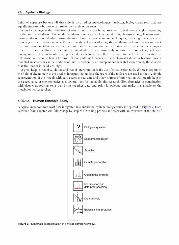
fields of expertise because all three fields involved in metabolomics (analytics, biology, and statistics) areequally important but none can solve the puzzle on its own.
A final challenge is the validation of results and this can be approached from different angles dependingon the aim of validation. For model validation, methods such as Jack-knifing, bootstrapping, leave-one-outcross-validation, and double cross-validation have become common techniques, reducing the chances ofreporting artifacts as biomarkers. From an analytical point of view, the validation is found by tracing backthe interesting metabolites within the raw data to ensure that no mistakes were made in the complexprocess of data handling or that internal standards (IS) are mistakenly reported as biomarkers, and withhaving only a few metabolites as potential biomarkers the effort required to perform identification ofunknowns has become less. The proof of the pudding however is the biological validation because once amodeled mechanism can be understood and is proven by an independent repeated experiment, the chancesthat the model is valid are high.
A great help in model validation and model interpretation is the use of visualization tools. Whereas experts inthe field of chemometrics are used to interpret the models, the users of the tools are not used to that. A simplerepresentation of the models with easy access to raw data and other sources of information will greatly help inthe acceptance of chemometrics as a general tool for metabolomics research. Bioinformatics in combinationwith data warehousing tools can bring together data and prior knowledge and make it available to themetabolomics researcher.
4.09.1.4 Human Example Study
A typical metabolomics workflow integrated in a nutritional system biology study is depicted in Figure 2. Eachsection of this chapter will follow step-by-step this working process and start with an overview of the state of
? Biological question
Experimental design
Sampling
Sample preparation
Quantitative profiling
Identification anddata preprocessing
Data analysis
Biological interpretation
Figure 2 Schematic representation of a metabolomics workflow.
284 Systems Biology

the art of the different steps involved in the nutritional metabolomics and systems biology workflow. This willbe focused on the application of chemometrics in this research field. Each section will end with the demonstra-tion of how the different topics were applied in a human intervention study as published by Wopereis andcoworkers21 and Rubingh and coworkers.22 The main focus of the example study was to demonstrate andquantify the consequence of an antiinflammatory intervention by the antiinflammatory compound diclofenacon metabolism in mildly overweight subjects with low-grade state of inflammation. Different analyticalmethods were used for the detection of high- and low-abundant plasma metabolites to obtain a comprehensivepicture of metabolic changes induced by this mild antiinflammatory drug intervention.
4.09.2 Study Setup
4.09.2.1 Study Design
Basically, two main types of design are being applied in clinical trials, namely a parallel design and a crossoverdesign (see Figure 3). In a parallel design, at least two groups of people are followed up in time, where eachgroup gets a treatment. The intervention effect is defined as the difference in the parameter of interest betweenstart and end of the intervention (treatment A in Figure 3). This difference occurring in the treatment period iscompared to the difference observed between start and end in the control treatment (treatment B in Figure 3).
In a crossover design, each person will undergo all treatments by switching treatment in each experimentalperiod including a control treatment period. The intervention effect is defined as the difference in theparameter of interest at the end of the intervention (treatment A in Figure 3) as compared to the sameparameter at the end of the control period (treatment B in Figure 3).
Each of the two designs has its own advantages and disadvantages. The parallel design has the advantage thatmany treatments can be included in the study and the subjects will be followed up during the same time period,so that specific changes over time, such as seasonal variations, will affect all experimental groups similarly. Thedisadvantage of this design is that the start condition of all experimental groups needs to be the same for thoseparameters that are being evaluated; in other words, randomization of the individuals to the various treatmentsneeds to be well controlled. This may be difficult if not all randomization factors are known or if there are manyrandomization factors to be considered. Other disadvantage is that interindividual variation is an importantsource of variation, which means that the statistical power is lower and that more individuals are needed in thistype of study.
The advantage of the crossover trial is that randomization will not be essential as it is in the parallel design,because all individuals will receive all treatments. Consequently, each individual will function as his or her owncontrol. Other advantage of this design is that the statistical power is higher in crossover trials as onlyintraindividual variation is to be considered. Therefore, less people need to be included in crossover trials.
The disadvantage of crossover trials is their longer duration, which may limit their feasibility. Potentiallyorder effects (a previous treatment affecting the following one) may play a role in crossover studies. However,
Parallel design
Cross-over design
Treatment A, n = ½x
Treatment B, n = ½x
Treatment A, n = x
Treatment B, n = x
Treatment A, n = ½x
Treatment B, n = ½x
Figure 3 Two main types of study designs in clinical trials.
Systems Biology 285

in case the treatment orders are randomized, for example, by using a Latin square, such problems are reduced toa minimum.
Variations on these two main intervention types exist, but are not discussed in this chapter.Choosing the right control may be difficult in a trial, specifically when the components have clear immediate
effects on behavior or when taste or other product characteristics are difficult to disguise. Furthermore, controlproducts may differ from the experimental condition only in the ingredients of interest.
Confounding of study outcomes may occur. Some of the potentially confounding factors include blinding,bad compliance, unwanted side effects, and insufficient power.
Clinical studies are preferentially blinded, which means that not only the participants do not know whichtreatment they receive (single blinded) but also those conducting the trial (double blinded).
Bad compliance may be a determining factor in observing no effect and therefore compliance marker may beevaluated or other means of maximizing compliance (more control, motivation, extra return products) need tobe considered.
One of the unwanted side effects occurs in diet-controlled studies. In these studies, caloric intake may beunderestimated, because part of the daily intake is simply forgotten. Also, physical activity needs to beestimated and needs to be compensated for. If not, applying a controlled diet may decrease caloric intake,reduce body weight, and lead to false conclusions because the observed effects are not mediated by theintervention but by weight loss.
Including too low numbers of volunteers may result in type 1 error (a positive effect of the intervention ispicked up) – the effect is due to chance – or type 2 error (no effect of the intervention is observed) – theabsence of an effect is due to limited statistical power. These errors can be quantified as theirprobabilities and need to be used to estimate the number of participants needed in a study preventingtype 1 and 2 errors.
In conclusion, many aspects of trial design need to be taken into account before one gets the most out of it,important among which are the type of design, power, and potentially confounding factors.
As stated earlier, nutritional metabolomics studies (and nutrigenomics studies in general) often haveto deal with large interindividual diversity (confounders). Furthermore, an organism under mild stress, forexample a nutritional intervention, attempts to maintain homeostasis and metabolic control, which makesit difficult to identify alterations in biofluids such as plasma. Furthermore, plasma and urine are biofluidsthat represent whole body metabolism, which means that the concentration of a metabolite is often thesum of different organs and thus the representation of several biological processes. These complexityissues might be addressed by designing an experiment that makes use of a ‘challenge test’. This experimentaldesign uses one or more stresses in such a way that an individual’s homeostasis is reversibly and safelyperturbated. This is based on the concept that the resilience of the system can be assessed after challenging orperturbing a homeostatic situation. Application of a metabolic perturbation in concert with metabolomicsmay identify a set of metabolites that are predictive of differences in response to the challenge. Althoughthis concept is new in nutrigenomics research, nutrient challenges are quite common in medical sciences.The oral glucose tolerance test (OGTT) is an example of a challenge test used for the diagnosis of type 2diabetes.23–25
4.09.2.2 Sampling/Sample Preparation
Both sampling and sample preparation can have a large influence on the variation within the final data usedfor modeling. In metabolomics-driven studies, the aim is to obtain a quantitative view on the status of thesystem at the time of sampling. The samples that are drawn from biological systems such as a microbiolo-gical fermentation or from body fluids such as blood or urine are highly susceptible to changes owing tobiological reactions taking place especially when the environment of the sample changes. It is thereforeessential that changes in metabolites are minimized during sampling and sample preparation. In themetabolomics society, it is recognized that there is a great need for standardization of sample collectionand preparation protocols for clinical studies. These standardized protocols should incorporate the optimalconditions from a metabolomics point of view as well as from a clinical point of view. Although it is
286 Systems Biology

impossible to prevent any changes in the samples during sampling, it is of utmost importance that samplingis carried out in a similar way for all samples in a study using standard protocols and that all steps arerecorded during the procedure.
Sampling can be both invasive (blood, cerebrospinal fluid (CSF), serum, tissues, intracellular metabolites inplants and microorganisms) or noninvasive (urine). Although the strategies of sampling may vary, the generalidea of sampling is to minimize the formation or degradation of metabolites due to remaining enzymaticactivity or oxidation processes. The time and method of sampling can have great influence on the reproduci-bility of the analytical sample. The storage of samples is also important as the continued freeze/thawing ofsamples can have a great influence on the stability and composition of samples.26–28
The sampling procedure depends strongly on the type of sample collected. Collection of plasma usuallyrequires the addition of an anticlogging agent, such as heparin, followed by centrifugation and subsequentstorage at�80 �C. For urine, the general procedure is to store the samples at low temperature (�20/�80 �C) inorder to inhibit metabolic reactions. Preservatives are in general not used for urine samples. Tissue samples aremostly freeze-dried and stored at �80 �C. Special precautions must be taken when reactive metabolites areunder study, like adding antioxidants to prevent oxidation of neurotransmitters.
Further sample preparation prior to analysis is mainly determined by the analytical method used. For globalprofiling methods, such as nuclear magnetic resonance (NMR) spectroscopy, liquid chromatography-massspectrometry (LC-MS), or gas chromatography-mass spectrometry (GC-MS), sample preparation is minimizedin order to retain as many metabolites as possible in the sample. In many applications, no further isolation ofmetabolites from the sample matrix is performed and samples are diluted and analyzed directly or afterchemical derivatization. For example, the analysis of biofluids by NMR requires no or only very limitedsample preparation.26,29,30 The same is true for the analysis of urine by LC-MS.28,31–34 The analysis of plasmaor tissue by MS-based methods usually requires protein precipitation and/or extraction of (certain classes of)metabolites. GC-MS analysis used in metabolomics includes chemical derivatization by oximation and silyla-tion.35,36 In certain cases, especially for low-abundant metabolites, further isolation of metabolites is necessaryusing solid-phase extraction (SPE) or liquid–liquid extraction (LLE). As said in the beginning of this section,sample preparation can have a large influence on the variation within the final data. It is therefore necessarythat every step in the sample preparation is validated as much as possible using, for example, stable isotope–labeled standards or quality control (QC) samples.
4.09.2.3 Analytical Measurements
The ultimate goal of metabolomics is the quantitative analysis of all metabolites in a sample. This isdramatically more complex than analyzing the genome or the proteome. This is due to the number ofmetabolites that constitute the metabolome as well as their structural and compositional diversity. Moreover,the concentration range to be covered in metabolomics is also extremely large. Comprehensive analysis of themetabolome thus requires analytical techniques and instruments that offer high resolving power, sensitivity,and dynamic range. This is a major challenge and therefore a lot of research is done to improve analyticalmeasurements in metabolomics, which is reflected in the numerous reviews on this subject in the recentliterature.29,34,36–47
Numerous analytical platforms have been used for metabolomics studies, such as NMR, Fourier transforminfrared (FT-IR) spectroscopy, and MS using flow injection or coupled to separation techniques. Theadvantages of NMR are the minimal requirement for sample preparation, the nondiscriminating and non-destructive nature of the technique, and the potential for high-throughput analysis.
The major disadvantage is the fact that only medium- to high-abundant metabolites are detected. Moreover,the identification of individual metabolites based on chemical shift signals is very difficult. MS-based metabo-lomics offers high selective and sensitive analysis and the potential to identify metabolites. However, MS-basedtechniques usually require sample extraction, which can cause metabolite losses and discrimination of meta-bolite classes. Also, very low-abundant metabolites can not be analyzed by MS-based profiling methods.
The chemical diversity of metabolites exceeds the span of any analytical method. Application of a singleanalytical method in metabolomics studies will therefore give only limited information. It is mandatory tocombine different analytical methods into an overall metabolomics platform to improve the metabolite
Systems Biology 287

coverage.48–52 GC-MS, LC-MS, and NMR-based metabolomics platforms are mostly used for the globalprofiling and quantification of biochemical changes.53,54 At the broad level, metabolomics platforms that aredeveloped in the context of a specific compound class may be used. Mostly, LC-MS-based techniques are usedfor this goal. Lipidomics platforms, for example, are specifically developed for the analysis of lipid biochemicalpathways.55 In addition, approaches have been described for the analysis of oxylipids,56 acylcarnitines,57 etc.Finally, at the focus level, very specific analytical platforms that often detect signaling molecules available inthe lowest concentration ranges have been developed. The (trace)-element status for example can be monitoredusing induced coupled plasma (ICP)-MS58 and neutral eicosanoid profiles can be generated via LC-MS/MSanalysis.59
Figure 4 illustrates an example of such a metabolomics platform including global profiling methods based onNMR, GC-MS, and LC-MS for relatively medium- to high-abundant metabolites, a collection of class-targeted profiling LC-MS methods for some specific classes of metabolites and metabolites with lowerabundance, and target LC-MS/MS methods for specific low-abundant metabolites. These methods cover awide range of different classes of metabolites, with the total number of distinct metabolites being in the order of60–800.48 Often not all methods are used but a selection is made based on prior knowledge, sample volume,time schedule, and budget constraints.
The analysis of the metabolome in body fluids has been approached via other techniques as well as GC incombination with flame ionization detection (FID) for the profiling of the lipid domain, which is a veryquantitative detection strategy.60 Other examples are LC coupled to electrochemical detection (ECD), allow-ing the detection of metabolites involved in neurotransmitter pathways and pathways involved in oxidativestress, and LC using diode-array and fluorescence detection.61,62 Most or all of these technical platforms arealready familiar in the field of pharmacology and toxicology. The difference in metabolomics used in differentresearch fields lies not in the platforms, but rather in the specific way in which these analytical tools are applied,the samples used, and the chemometric methods applied to the data.
Reports of the plasma metabolome composition are widely variable but range from 10 to 30 thousand smallmolecules. The coverage today is still limited, with NMR typically covering the mg ml�1, mg ml�1, and at bestthe high ng ml�1 range measuring in the order of 300 – maximum 500 – components for a 600 MHz to massspectrometric applications covering also the ng ml�1 and pg ml�1 range when applied on focused metaboliteclasses. The strength of NMR is typically its power of quantification for several high-concentration compoundclasses, but nonpolar metabolites such as lipids and low-abundant metabolites such as neurotransmitters, whichare very important in many diseases and in nutritional studies, are not measurable. Currently, MS-basedmethods are mostly used in metabolomics studies, often in combination with separation methods, that is, LC-MS and GC-MS. Resolution of these methods improves dramatically by using high-resolution mass spectro-meters, for example, time-of-flight (ToF) and Fourier transform-ion cyclotron resonance (FT-ICR). Thecoupling of separation and MS increases the resolving power, dynamic range, and sensitivity. Sensitivity is very
Met
abol
ic p
rofil
e
Global profilingNMR profile
UPLC-MSLC-MS derivatized
GC-MSGCxGC-MS
Multi-targetanalysis
Trace elements (ICP-MS),endocannabinoids, oxilipids, steroids,
neurotransmitters (LC-MS/MS)
Class-targetedprofiling
Bile acidsLC-FTMS
Nucleosides,Acyl CoA,
phosphorylatedLCMSC
linic
al s
ampl
es
PeptidesLC-MS
Fatty acidsLC-FTMS/GC-MS
Amino acidLC-FTMS
Glycerolipids,Sphingomyelins, Ceramides, Cere-brosides LCMS
Figure 4 Example of a comprehensive metabolomics platform combining global and targeted analytical methods.
288 Systems Biology

important in metabolomics for including low-abundant metabolites and for working with limited samplevolumes. The major challenges for MS-based methods are quantification and identification, which will bedescribed later.
Besides good coverage and sensitivity, it is of utmost importance that the analytical methods used inmetabolomics studies show good analytical performance. The statistical analyses that are performed on thefinal data are often complicated especially when longitudinal sampling and different subgroups are included. Asa result, the order in which samples are measured within an analytical series of measurements is critical, whilevariations within the instrument and/or method can easily induce differences or trends that can be mistaken forbiological effects.
4.09.2.4 Quality Control
Variation in sample preparation and analysis can easily induce differences or trends that can be mistaken forbiological effects. The magnitude of this problem is proportional to the scale of the study. Small-scale studies,which contain only a small number of samples in a single batch of experiments, may only suffer frominstrumental drift for example due to ion source contamination. Owing to the use of IS, much of theinstrumental drift and offset in between series can be corrected for but the IS are not available for eachindividual metabolite, and hence the remaining drift has to be taken into account. Large-scale studies, such asnutritional metabolomics studies, are even more challenging while these studies result in large time intervalsbetween the analyses of different batches of samples from the same study sample set.55 Sometimes, parallelinstruments of the same type are used in the same laboratory or even in different laboratories. All these aspectswill induce variation for which corrections should be made. Relevant biological information can be obtainedfrom these studies only if the reliability, repeatability, and reproducibility of the different steps in the workfloware excellent.
The only way to achieve this is to develop validated protocols for sample preparation and analysis.32,48,63 Allsamples should be treated in a similar way in order to be able to compare samples within a study. Validation ofthe different steps in sample preparation can be carried out using standard addition experiments and stableisotope–labeled standards, and corrections, for example recovery, can be made after analysis. Analyticalmethods should be used only if they are extensively validated.31,33,35 Furthermore, standardized analysisdesigns should be applied using QC samples26,31–33,63 or preferably biological calibration samples,48 calibrationstandards for quantification of specific metabolites and randomized study samples. Which randomization is theproper method depends on the study design and the way the data analysis is performed, which calls for an earlychoice of the data analytical method to be used. QC samples are used to rigorously monitor the performance ofthe method.32 These samples are preferably pooled study samples that are analyzed at the beginning, end, andrandomly through the run. In practice, these QC samples are used only qualitatively to determine for examplewhether a batch of experiments failed based on preset acceptance criteria. Recently, Van Der Greef et al.48
described an alternative approach using biological calibration samples and this can be used to quantitativelycorrect for intrabatch temporal trends and remove systematic batch-to-batch differences. Although with thisapproach no real quantitative data are obtained, that is, absolute concentration, it is at least possible to compareresponses of metabolites between different samples analyzed in different batches. In this way, analyticalvariation is removed almost completely and will thus not hamper statistical analysis of the final data.
Standardization at an international level is needed in order to be able to improve the universal significance ofdata generated from different studies at different sites and this will improve the overall understanding ofcomplex biological systems.
4.09.2.5 Human Example Study: Design and Measurements
4.09.2.5.1 Design and samples
The study was designed as a double blind, randomized, parallel trial, in which subjects were treated withdiclofenac (n¼ 10) or placebo (n¼ 10). Randomization of subjects to treatment groups was restricted by thelevels of high-sensitivity C-reactive protein (hsCRP), body mass index (BMI), fasting glucose, and age. Subjectsconsumed one capsule (placebo or 50 mg diclofenac) �1 h before breakfast, lunch, and dinner for 9 days.
Systems Biology 289

Subjects were instructed to keep their habitual diet during the study. Nineteen men completed the study. Oneperson dropped out on the first day of the study for reasons unrelated to the study. The metabolomics approachwas applied not only in fasting (homeostatic) conditions, but also on multiple time points during an oral glucosechallenge test (OGTT). This is based on the concept that the resilience of the system can be assessed afterchallenging or perturbing a homeostatic situation. Application of a metabolic perturbation in concert withmetabolomics may identify a set of metabolites that are predictive of differences in response to the challenge,which is measured as a change in time to return to baseline concentrations. Blood samples were taken after anovernight fast on days 0, 2, 4, 7, and 9. Subjects underwent an OGTT on days 0 and 9. Blood samples were takenjust before (0 min) and 15, 30, 45, 60, 90, 120, and 180 min after the administration of the glucose solution (70 g).Figure 5 shows the study design and time points at which metabolome measurements were made.
4.09.2.5.2 Metabolomics measurements
LC-MS and GC-MS techniques were applied on the plasma samples. LC-MS was used to measure thecompound classes lipids (LC-MS lipids), free fatty acids (LC-MS FFA), and polar compounds (LC-MSpolar).55,64 Plasma GC-MS was applied to screen for metabolites on the global level.35 In total, 19 plasmasamples per person were measured on all 4 metabolite platforms, which is a total of 361 plasma samples.Furthermore, a QC sample was prepared by pooling plasma from all subjects. The pool was divided into 10 mlaliquots and these were extracted the same way as the study samples. The QC samples were placed at regularintervals in the analysis sequence (one QC after every 10 samples). The QC samples serve two purposes. Thefirst is a regular QC sample to monitor the LC-MS response in time. After the response has been characterized,the QC samples are used as standards of unknown composition to calibrate the data.48 The LC-MS lipidsplatform detected a total of 61 different lipids, the free fatty acid platform a total of 14 fatty acids, and theLC-MS polar a total of 130 polar compounds. The GC-MS platform detected a total of 137 metabolites. Thus,in total, about 340 different plasma metabolites were analyzed per subject.
4.09.3 Data Preprocessing
4.09.3.1 Signal Alignment
The information acquired with instrumental measurements such as GC-MS, LC-MS, and NMR is sometimes usedas is, without extraction of individual peaks based on the total ion current (TIC) of the GC-MS and LC-MS datafiles or the individual spectra of the NMR measurements.65 Owing to variations within the measurements such aspH differences or instrumental changes (shortening of the analytical column in GC measurements, variations ineluent composition for LC instruments, etc.), the position of the individual peaks with the same identity within thedifferent data files will vary and correction is required even when the total signal (profile) is used for data analysis. Inthat case, alignment methods such as correlation optimized warping (COW) are applied (see Chapter 2.06). For
Placebo or diclofenac treatment
Day 0 Day 2 Day 4 Day 7 Day 9
c
c
b b
15 30 45 60 90 120 180 minutes
Blood samplingduring OGTT
Blood samplingafter overnight fast
b ba
cba
Figure 5 Overview of the study design of diclofenac study and time points at which the metabolome was measured.
290 Systems Biology

instance, in GC analysis, a small part of the GC column is removed after a certain number of measurements toprevent unwanted effects on the analysis results owing to fouling of the column. Shortening of the column will resultin a distinct shorter retention for all the metabolites and a simple additive correction procedure will solve thisproblem. For NMR, alignment is mostly performed after peak extraction where each peak can have a different shiftbehavior owing to variations in the pH of the sample. It should be remembered that with NMR the whole sample ismeasured at once without prior separation of the individual compounds. It would be possible to perform LC-NMRmeasurements in which prior to the NMR measurements a separation by means of LC is performed, but thismethodology is not common practice yet in metabolomics research (For more information, please see Chapter 3.04).
4.09.3.2 Peak Extraction
Metabolomics measurements can be performed on different instruments (or platforms, in the metabolomicsjargon). Mainstream methods are NMR, GC-MS, and LC-MS. All three methods have their own characteristicsand require preprocessing to clean up the data. For NMR, this comes down to correcting for peak shifts. ForGC-MS and LC-MS, the characteristics of the clean data change depending on the type of preprocessing.Essentially, there are three ways to preprocess GC-MS and LC-MS data: target analysis, peak-picking, anddeconvolution. In target analysis, a specific m/z channel is sought in the MS domain that is specific for ametabolite. Then the associated chromatographic peak can be integrated and used as pseudo-concentration.Each metabolite is represented by one variable in the final data table.
In peak-picking, first the m/z traces containing meaningful information are selected (e.g., with CODA66 orImpress67) and then the peaks in the selected ion traces are integrated to obtain single-intensity measures forcomplete peak profiles. This results in a data table in which one metabolite is represented by different variables(peaks representing different ions as present in the mass spectrum).
In deconvolution, the coeluting peaks in the chromatograms are mathematically resolved whereanalytical resolution of the peaks remained incomplete. Multiple overlapping peaks representing differentmetabolites are deconvoluted. After that, the resulting pure chromatographic peaks are integrated. Thisresults in a table of areas per chromatographic peak (¼metabolite), representing pseudo-concentrations.A second table is produced as well containing the mass spectral information, which can be used formetabolite identification (For more information, please see Chapter 4.13).
From the above descriptions, it is clear that different data structures arise for GC-MS and LC-MS dependingon the type of preprocessing. In the target and deconvolution case, a single variable in the data table alsorepresents a single metabolite. For the peak-picked data (and also for the NMR data), multiple variables candescribe one metabolite. The latter means that there are two types of correlation in a data table: the ‘analytical’correlation (more variables for the same metabolites) and ‘biological correlation’, the correlation betweenmetabolites induced by the underlying biology. Peak-picked data sets are usually megavariate, but do notnecessarily contain more metabolites than a smaller targeted or deconvoluted data set.
4.09.3.3 Peak Alignment
Given an optimal instrument and standardized samples (same pH for instance in the case of NMR measure-ments), it should be possible to obtain intensities of the same chemical entities within different samples at thesame retention time (chromatography) or the same chemical shift (NMR). However, the situation is not optimaland some differences between samples exist and as a result after peak extraction from the raw data, equalchemical entities are reported at different retention times or chemical shifts. To correct this, multiple methodshave been developed. Chapter 2.06 of this book deals in great detail with the subject of alignment.
4.09.3.4 Quantification
Metabolomics comprises the quantitative analysis of metabolites. However, to obtain the actual concentrationsof metabolites in samples, analyses using stable isotope–labeled IS and calibration standards are necessary forevery metabolite. This is possible for target analysis, but quite a challenge for global profiling methods, if not
Systems Biology 291

impossible. For known metabolites, in global profiling methods it is possible to use stable isotope–labeled IS inorder to obtain quantitative data. However, generally, these methods are able to measure hundreds ofmetabolites, many of them being unknowns. Practically, class-targeted and global profiling analysis is nothingmore than recording the response of substances in samples in which the response is only a measure ofconcentration. In the ideal case, the peak areas for the same metabolite in different samples should be directlycomparable with each other on a relative scale. However, as mentioned earlier, the response is determined notonly by the actual concentration, but also by various other factors. These factors should be prevented orcorrected for in order to be able to compare metabolite responses. Peak extraction of metabolomics datagenerally leads to raw peak areas of metabolites. These peak areas should then be corrected for the biological(e.g., biomass, creatinine for urine) and analytical variation (intrabatch drifting and batch-to-batch differences)using biological calibration samples48 to obtain relative peak areas that can be compared between samples indifferent batches. Using calibration standards, known metabolites can then be at least semiquantified.Quantitative aspects are even more challenging in large-scale human studies, such as nutritional metabolomicsstudies, because these studies result in large time intervals between the analyses of different batches of samplesfrom the same study sample set. In metabolomics, it is often sufficient to know whether there are metabolitesthat increase or decrease in concentration as a result of a specific treatment or illness and the identity of thesemetabolites. However, if these metabolites are present and identified, the next question is often what the exactconcentration is in order to compare the results with other results from clinical studies.
4.09.3.5 Human Example Study
The raw analytical data with the diclofenac study were processed with homemade comprehensive peak-pickingsoftware Impress.68,69 This software is able to extract peaks from multiple data files and perform alignment ofthe peaks. Still, manual setting of parameters is required and to circumvent subjectivity of the preprocessing theproduced peak list was used only to extract all possible features from the total set of data files. From theextracted features, all isotopes were removed, resulting in the removal of multiple entries of the samemetabolite and a data set was obtained containing only one entry per metabolite. These features were thenentered into the XCalibur software version 1.4 (Thermo Electron Corp., San Jose, CA, USA). Within thissoftware, retention time windows and mass windows are entered for each metabolite, and for each data file thematching peak intensity is reported.
Data of each subject were corrected for the recovery of the IS for injection. Batch-to-batch differences in datawere removed by synchronizing the medians of QC samples per batch. QC samples are produced by poolingtrue samples from the study forming a large quantity of one composite sample that contains all metabolites thatare also present in the individual sample. The theory is that repeated measurements should result in the sameanalytical result and that deviations from that assumption are due to analytical effects. For each metabolitewithin an individual sample, a matching metabolite is available within the pooled QC sample. After each 6th or10th study sample, a QC measurement is performed, depending on the analytical method. The measuredintensities in the first batch are taken as reference batch and the QC measurements in each consecutive batchare matched toward those QC measurements. Different ways of correction are possible depending on the typeof deviation within the measurements of which a simple offset is the simplest one.
For all platforms, duplicate measurements were combined into a single measurement. When both analyticalduplicates had a zero value or when both had a nonzero value, measurements were averaged, whereas the singlevalue was taken when only one of the duplicates was above zero.55 To avoid trivial results, data wereadditionally cleaned up by removing glucose-related metabolites and IS isotopes in the LC-MS polar dataand glucose metabolites in the GC-MS global data set.
4.09.4 Data Analysis
Data from metabolomics studies have some specific characteristics that are different from other types of data.Many of the metabolomics-specific issues have already been mentioned in Section 4.09.1.3. Additional issues toconsider are data fusion, scaling, and centering.
292 Systems Biology

Metabolomics measurements are often performed on the same samples using different platforms in order toobtain an as comprehensive view on the sample composition as possible. Owing to the different characteristics ofthe instruments and different data preprocessing strategies used, combination of data sets is not straightforwardand calls for data fusion strategies.70 Data sets obtained from different instruments have unequal noise character-istics, which can be due to, for instance, chemical reactions within the ion spray in LC. Another aspect to take intoaccount when combining data sets from different instruments is whether the relation between measured intensityand true concentration is comparable between instruments. This is especially of concern when combining datasets from instruments with different working mechanisms such as NMR and MS. The final concern is the methodused to convert raw data into peak tables. One method will result in peak tables in which each metabolite isrepresented by one variable (target analysis and deconvolution), whereas another method will result in a peaktable in which metabolites are represented by multiple variables (e.g., peak-picking). The process of combining orfusing the data is completely context dependent and will not be discussed in detail here. Needless to say, fusingdata of different platforms only aggravates the problem of low sample-to-variable ratios.
Another special issue is scaling and centering within metabolomics data analysis especially where differentgroups and dose and time effects are included within one study. In two-way analysis scaling and centering arequite straightforward, whereas in multiway analysis they are more complicated, because centering across orscaling within a certain mode might disturb prior centering and/or scaling steps.71–73
4.09.4.1 Metabolomics-Specific Modeling
Many if not all chemometrical modeling techniques have been used to process data obtained from metabolomicsexperiments. While metabolomics studies often suffer from a large number of variables (p) in comparison to thenumber of objects or samples (n), certain methods such as multiple linear regression (MLR) will not fulfill thepurpose of metabolomics modeling. Regularization methods such as ridge regression (RR), support vectormachine (SVM), and least absolute shrinkage and selection operator (LASSO) are suitable for solving the problemof (near) colinearity, which results in unstable models with highly variable regression coefficients (For moreinformation, please see Chapters 4.08, 4.12, 3.01 and 3.05). However, the general method used for a first view ofmetabolomics data sets is still the principal component analysis (PCA), enabling a general view of the structure ofthe data at hand (For more information, please see Chapter 2.13). Gross errors, outliers, and a first idea of theamount of clustering are quickly discovered looking at the PCA score plots. Likewise, partial least squares (PLS) isused to correlate the sample composition to a kind of phenotype such as the yield of a fermentation process (Formore information, please see Chapter 3.01). PCA and PLS are well suited for two-way data sets, whereasstructured data need to be processed with methods such as variance (ANOVA)-simultaneous component analysis(ASCA) and n-PLS, which can handle the underlying structure in the data sets. For example, when at the sametime healthy versus diseased and a development in time of the metabolic changes are to be traced, the structure ofthe study design needs to be included to ensure that the different sources of variation are not mixed up. Inclusionof the experimental design into model assessment also helps in obtaining results that can be interpreted moreeasily (For more information, please see Chapters 4.05, 4.12, 1.02, 2.23, and 3.03).
In many metabolomics studies, the general question is to find metabolites that are able to discriminate betweenhealthy and diseased or between treated and untreated patients. Once the metabolites are found that arediscriminating between the groups, biological interpretation using genetic information or pathway informationcan be performed. Examples of suitable methods for classification are PLS-discriminant analysis (PLS-DA) in thecase of a two-way data structure and n-PLS-DA for multiway data structures.
A new direction that is being developed within metabolomics research is to build models using priorknowledge. Prior knowledge can be the nearness of metabolites within a metabolic pathway and therebytheir simultaneous reaction to disturbances within the pathway. Among others, methods that can be used toincorporate prior knowledge are Grey component analysis (GCA)74 and Bayesian statistics (For more informa-tion, please see Chapters 2.23, 3.23, and 2.03).75
4.09.4.2 Model Validation
Although it is impossible in many cases to expand the number of experiments of metabolomics studies owing tocosts or for ethical reasons in the case of animal or human studies, statistical resampling techniques need to be
Systems Biology 293

applied to perform model validation. In applications where the availability of samples is less problematic, datasets can be subdivided into training sets and validation sets. This is not the case in metabolomics and techniquessuch as double cross-validation (2CV) can be applied;76,77 it is currently the best method to mimic validationwith a true test set. Using 2CV, cross-validation can still be used to find a good estimate of the prediction errorwithout having to define a dedicated data set for model building, model validation, and estimation of predictionerrors. Determining the tunable parameter (e.g., number of latent variables (LVs) in PLS) with cross-validationis part of the procedure to build a model. The entire modeling procedure has to be cross-validated in order toobtain the prediction error. The double cross-validation consists of two nested cross-validation loops.The modeling procedure, including the cross-validation that determines the tunable parameter, forms theinner loop. The cross-validation for the error estimation takes place in the outer loop.
Biological and analytical validations of the model results are as important as the statistical validation.Variables that appear to be of importance, as deduced from statistical analysis, should be traced back in theanalytical data to ensure that these variables are not just artifacts for instance due to extraction procedures. Also,biological validation as far as information is available about the variables should reveal whether certain effectsas explained within the statistical model can be explained. Examination of the feasibility of the statistical modelscan be based upon metabolic pathways or upon thermodynamic information.78
4.09.4.3 Human Example Study
PLS-DA79 was used to identify metabolites that differed in their change between days 0 and 9 in fastedconditions between treatment groups (Figure 5, analysis a). As the interest was in intraindividual differencesbetween days 0 and 9, the X-block was defined for each metabolite platform by subtracting the day 0 valuesfrom the day 9 values, which removed interindividual differences.80
For the identification of metabolites that differed in their change caused by the treatments betweendays 0, 2, 4, 7, and 9 time course and days 0 and 9 OGTT time course, the multiway generalization ofPLS-DA was used (n-PLS-DA).81–83 In this way, metabolites can be identified that differ in changes overtime between the treatment groups, by creating a so-called three-way matrix of size 19� J�T, where19 is the number of subjects, J is equal to the number of metabolites of a particular platform, and T isequal to the number of time points, which were either days 0, 2, 4, 7, and 9 (Figure 5, analysis b) or thetime points after glucose administration on days 0 and 9 (Figure 5, analysis c). For the statistical analysisof the OGTT time-course data, the day 0 data were subtracted from the day 9 data, removinginterindividual differences. The GC-MS global and LC-MS polar data sets were centered across subjectsand followed by scaling within the metabolite mode J, whereas the LC-MS lipids and fatty acids datasets were centered only across subjects. The centering step was performed to remove constants betweenthe subjects, whereas scaling within the metabolite mode resulted in standardized metabolites. Byperforming the scaling step after the centering step, the prior centering remained unaffected.72,73,83
In (n-)PLS-DA, a Y variable containing class membership information is correlated to the data block X. Inthe present study, the metabolic response (X) is related to treatment groups; hence y is not a continuousparameter as in regular regression, but a dichotomous vector containing the treatment group membership. Thesubjects who received the placebo treatment were assigned to class ‘0’ and the subjects who received diclofenacwere assigned to class ‘1’.
The following model was used in the analysis of the 0, 2, 4, 7, and 9 days time course:
T ¼ XV
X ¼ TG WM �WK �WJ� �9þEx
y ¼ TBþ ey
max cov tc ; yc – 1ð Þ� �
; c ¼ 1; . . . ;C
wMc ;w
Kc ;w
Jc
ð1Þ
where V is a matrix of weighing coefficients which can be written in terms of W, G is the core array, B is theregression matrix for regressing y on T, and Ex and ey are the residuals of the model for X and y, respectively.71
294 Systems Biology

For the analysis of the OGTT time course, the multilevel variant of multiway PLS-DA was used. As theinterest is in intraindividual differences specifically, the interindividual variation can be removed by subtract-ing the day 0 data from the day 9 data. The multilevel multiway model was created, which regresses parametery containing the treatment group membership to the changes in metabolic response between days 0 and 9,X9�X0 (size I� J� K). The model used was adapted as follows:
T ¼ X9 –X0ð ÞVX9 –X0ð Þ ¼ TG WM �WK �WJ
� �9þEx0–x9
y ¼ TBþ ey
max cov tc ; yc – 1ð Þ� �
; c ¼ 1; . . . ;C
wMc ;w
Kc ;w
Jc
ð2Þ
The creation of the X-block that was used for n-PLS-DA modeling is illustrated in Figure 6. First of all, athree-way matrix X0 of size 19� J� 8 was created. This matrix contained the metabolic data of day 0,determined at eight different time points for each subject. A matrix X9 of the same size was also created,containing similar information for the day 9 measurements. Finally, the X0 matrix was subtracted from the X9
matrix and this X-block was used for data analysis.Cross-validation was used to validate the (n-)PLS-DA models, using a ‘leave-one-out’ cross-validation
scheme.84 Data of one subject were left out in the first cross-validation step, a (n-)PLS-DA model wasbuilt, and the treatment class membership of the subject who was left out was predicted. This wasrepeated until all 19 subjects were left out once. The error rate of the model was determined bycomparing the original class membership and the predicted one. The optimal number of LVs wasdetermined based on the minimum value of the error rate. The final fit of the model was made usingthe number of optimal LVs. (n-)PLS-DA models for which an error rate was found below 35% wereoptimized by performing metabolite selection based on a jack-knife approach.84 Data of one subject wereleft out and a (n-)PLS-DA model was made using the same number of LVs as those used for the finalmodel. This was repeated until all 19 subjects were left out once. This resulted in 19 sets of regressioncoefficients, the standard deviation of which was used to determine the relative standard deviations(RSDs) of each regression coefficient. Only those metabolites that had an RSD of less than 50% wereincluded in the new data set, which was used to build a second (n-)PLS-DA model. Metabolitesthat contributed to treatment differences were identified based on absolute regression coefficients ofthis second model.
n
jk
X9
n
jk
n j
k
n j
k
n j
k
placebo
diclofenac
placebo
diclofenac
Original data sets Create three-way matrices Subtract day 0 from day 9
X9
X0X0
X9-0
Figure 6 The creation of the X-block that was used for multilevel n-PLS-DA modeling.
Systems Biology 295

A permutation test was performed to test whether the treatment differences were indeed truedifferences. One thousand dichotomous y vectors were randomly created using the same proportion ofzeros and ones as the vector that was used for modeling. For each random vector, a multilevel n-PLS-DA model was made using the same ‘leave-one-subject-out’ cross-validation approach and the error ratewas calculated. A distribution was made of all thousand error rates and the error rate for the originalmodel was compared to this distribution, which resulted in a p-value for the significance of treatmentdifferences. All analyses were performed using Matlab Version 7.0.4 R14 (The Mathworks, Inc.) and then-way toolbox version 2.11.85
4.09.4.3.1 Results
Table 1 shows the results of these multivariate analyses of the different data sets derived from the fourmetabolomics platforms.
Comparison of the fasting state metabolomes between subjects treated with placebo and diclofenac on day 9compared to day 0 resulted in PLS-DA models (Figure 5, analysis a) with high error rates, indicating nosignificant difference in fasted plasma samples.
Extension of the n-PLS-DA models with the metabolomics data of the plasma samples taken in fastedconditions on several intermediate days (Figure 5, analysis b) during the intervention for the variousmetabolomics platforms also resulted in high error rates. This confirms that no significant metabolomicchanges could be detected between subjects treated with placebo and diclofenac at the fasted (homeostatic)condition.
Metabolic perturbation by the OGTT considerably improved the metabolomics-based differentiationbetween the treatments. The n-PLS-DA models on plasma samples taken in an eight-point time course afterglucose administration of subjects on day 9 versus day 0 (Figure 5, analysis c) resulted in improved error ratesfor all metabolomics platforms compared to PLS-DA and n-PLS-DA models based on plasma in fastedconditions, between the control and antiinflammatory treatment. The n-PLS-DA models for metabolomedata from GC-MS global, LC-MS polar, and LC-MS lipids were optimized by using a jack-knife approach. If asubject is left out and the regression coefficient changes a lot, this will result in a relatively high RSD for thatparticular variable. A variable with a high RSD was considered to be unstable and hence unreliable forexplaining the differences in response between the placebo and the diclofenac group. The n-PLS-DA modelsafter jack-knifing for GC-MS global and LC-MS polar metabolome data resulted in models with error rates of10.5 and 5.0% respectively, indicating that the GC-MS global model and the LC-MS polar model misclassifiedrespectively only 2 and 1 persons out of 19. The model of the LC-MS lipids data set resulted in a model with anerror rate of 16%, indicating that 3 out of 19 subjects were misclassified. For the LC-MS polar model, forexample, 10 of the variables that appeared in the top of the model based on the original 120 variables
Table 1 Results of multivariate data analysis, expressed as error rates, of various metabolomics data sets
Method GC-MS global (137 a) LC-MS polar (130 a) LC-MS lipids (61 a) LC-MS FFA (14 a)
PLS-DA
Day 9 vs. day 0
42.0% 53.0% 37.0% 37.0%
n-PLS-DA
Days 0, 2, 4, 7, and 9
57.0% 42.0% 52.5% 47.0%
n-PLS-DA
Day 9 vs. day 0; 0–15–30–45–60–90–120,
and 180 min
31.5% 31.5% 21.0% 31.5%
n-PLS-DA after metabolite selection
Day 9 vs. day 0; 0–15–30–45–60–90–120,
and 180 min
J¼ 77
10.5%
J¼ 31
5.0%
J¼ 25
16.0%
NA
a Number of metabolites.
Note: Metabolite selection was applied only if the error rate of the original model of the complete data set was below 35% and
the data set contained more than 50 metabolites. NA, not analyzed.
296 Systems Biology

overlapped with the model using 31 variables. So, essentially the same information could be described usingfewer variables, illustrating the fact that many variables were unimportant for the model. Overall, it wasconcluded that significant metabolomic changes due to the treatment could be detected only in the metabo-lomics data of the OGTT time course.
4.09.4.3.2 Statistical interpretation
The optimized LC-MS polar model will be used for the statistical interpretation of the results from themultilevel multiway models. The multiway regression model resulted in a regression matrix of size J �� K, inwhich J � is the number of variables after variable selection. To determine the variables that contributed most totreatment differences, the regression coefficients were sorted by their absolute value in descending order pertime point K. For each time point, the first 10 variables were selected and used for interpretation. The selectedvariables are presented in Table 2.
The contribution of each variable to the treatment effect can be followed over time by investigating itsappearance in the list of parameters that contribute most to the differences between treatments. Somemetabolites were important over the whole range of time, whereas others were contributing only for acertain period of time. The variables that appeared in the top 10 for only one time point were consideredto be coincidently related to the treatment. Variables V01 and V02 will be used to illustrate furtherinterpretation.
V01 is an example of a metabolite that contributes to the response differences between treatments at eachmeasurement point, as illustrated by the light-gray shade in Table 2. This means that the response of thismetabolite between days 0 and 9 differed during the whole time course in subjects treated with diclofenaccompared to the placebo group. This effect is illustrated in Figure 7, in which the mean difference betweendays 9 and 0 response for V01 is plotted per treatment group. The placebo group had at fasting state (t0) a meanchange of about zero between days 9 and 0, whereas at the same time point the diclofenac group had a meandecrease of 2.5 units. The difference between treatment groups fluctuates between 1 and 2.5 units, dependingon the time point, but it remains quite stable over time. In Figure 8, the regression coefficient of this variable isplotted against the time. The same conclusion can be drawn toward this metabolite from this figure.
Variable V02 was only seen in the top 10 of contributing variables at 90 min and later of the OGTT, asillustrated by the dark-gray shade in Table 2. This metabolite was ranked 13 at t90 and therefore not included inTable 2 for this time point. The ranking at t0, t15, t30, and t45 was 21, 18, 29, and 26, respectively. So, after 1 h, thismetabolite differed in response to the challenge test between days 9 and 0 in subjects treated with diclofenaccompared to the placebo group. This effect is illustrated in Figure 9: The differences in response are more or lessthe same up to 45 min and around zero, whereas they deviate from t60 and later. In Figure 10, the regressioncoefficient of this variable is plotted against the time. There is no significant contribution to treatment differencesover the first 60 min of the curve. Only after an hour, this variable becomes more important.
For the interpretation of the results of this type of modeling, it must be kept in mind that the regressioncoefficients, which were used to rank the metabolites, are based on a model in which other metaboliteswere also included. So, each coefficient reflects the relation between the treatment group and that
Table 2 Overview of variables selected and used for interpretation
Ranking
Time point (minutes) 1 2 3 4 5 6 7 8 9 10
0 V01 V12 V51 V13 V48 V42 V53 V17 V27 V86
15 V31 V51 V44 V17 V12 V01 V15 V54 V59 V38
30 V01 V12 V51 V13 V17 V48 V42 V53 V86 V08
45 V01 V12 V17 V51 V13 V31 V08 V42 V48 V44
60 V01 V12 V13 V51 V17 V16 V08 V77 V48 V02
90 V54 V17 V77 V88 V76 V59 V53 V86 V16 V19
120 V48 V01 V08 V02 V13 V17 V36 V12 V16 V27
180 V01 V12 V17 V51 V13 V16 V08 V48 V02 V31
Systems Biology 297

particular metabolite, given the presence of the other metabolites that were used in that particular model.In Figures 8 and 10, the other metabolites are not taken into account, and hence these are univariateillustrations of multivariate results.
In Figure 11, the results of the permutation test are shown. The asterisk represents the error rate of the n-PLS-DA model that was made, whereas the histogram represents the distribution of error rates based on permutedclasses. In Figure 11(a), the results of the overall multilevel n-PLS-DA model are given, and in Figure 11(b), theresults of the optimized multilevel n-PLS-DA are given. The results for the overall model are very moderate(p¼ 0.472 5), but the treatment differences become more clear after optimization of the model (p¼ 0.005 9).
0 20 40 60 80 100 120 140 160 180–0.045
–0.04
–0.035
–0.03
–0.025
–0.02
–0.015
–0.01
–0.005
0
Reg
ress
ion
coef
ficie
nt
Time (min)
V01 (isoleucine)
Figure 8 Regression coefficients over time of a multilevel n-PLS-DA model for variable V01 – identified as isoleucine – thatcontributes to treatment differences at each time point of the time course.
0 20 40 60 80 100 120 140 160 180–3
–2
–1
0
1
2
3× 10⁵
Mea
n da
y 9
– da
y 0
Time (min)
V01 (isoleucine)
PlaceboTreatment
Figure 7 Mean change (�se) in metabolic response to the challenge test between days 9 and 0 for subjects on placebo and
diclofenac treatment, for variable V01 – identified as isoleucine – that contributes to treatment differences over the wholetime course.
298 Systems Biology

4.09.5 Metabolite Identification
4.09.5.1 Identification
The identity of statistically relevant metabolites in metabolomics studies is a prerequisite for biologicalinterpretation. The Human Metabolome Database (HMDB, www.hmdb.ca) is the most complete and compre-hensive database of human metabolites, containing records of more than 2000 endogenous metabolites.86,87
0 20 40 60 80 100 120 140 160 180–0.01
–0.005
0
0.005
0.01
0.015
0.02
Reg
ress
ion
coef
ficie
nt
Time (min)
V02 (glycine)
Figure 10 Regression coefficients over time of a multilevel n-PLS-DA model for variable V02 – identified as glycine – that
contributes to treatment differences only in the second part of the time course.
0 20 40 60 80 100 120 140 160 180–4
–2
0
2
4
6
8× 10⁵
Mea
n da
y 9
– da
y 0
Time (min)
V02 (glycine)
PlaceboTreatment
Figure 9 Mean change (�se) in metabolic response to the challenge test between days 9 and 0 for subjects on placebo and
diclofenac treatment, for variable V02 – identified as glycine – that contributes to treatment differences in the second part ofthe time course.
Systems Biology 299

Besides literature-derived data, the database also contains experimental metabolite concentration data com-piled from mass spectra and NMR analyses performed on urine, blood, and CSF. Furthermore, thousands ofNMR and MS spectra of purified, reference metabolites are collected. Besides knowing what metabolites arepresent in biofluids, it is important to know what metabolites can be analyzed with a specific analytical method.As explained earlier, analytical methods with different comprehensiveness can be applied for metabolomicsstudies. For target methods and target biomarker assays, it is exactly known which metabolites can be measuredand identification is not an issue. For class-targeted profiling methods, it is known which class of compoundscan be analyzed and databases for these methods can be made based on reference compounds and the HMDB. Ifunknown metabolites are detected in these methods, one already knows what type of metabolite it is. In mostcases, further identification using high-resolution MS and MS/MS is necessary, as will be explained further on.In global profiling methods, such as NMR and GC-MS, metabolites with different chemical structures can beanalyzed within a single method. An unknown peak in such a method is by all means a real unknown. For thesemethods, it is essential that databases are built based on reference compounds. If methods are standardized andwidely accepted, it is possible to build open-access databases, such as the Golm Metabolome Database(www.csbdb.mpimp-golm.mpg.de/csbdb/gmd/gmd.html) for GC-MS.88
Chromatograms of biofluids analyzed by global profiling methods will always contain unknown peaks. Foridentification of unknown peaks detected by LC-MS, the ideal strategy would be the isolation of the peak byfractionation of the LC eluent and subsequent structure elucidation using NMR and MS/MS, which can bedirectly coupled.89 However, as metabolites to be identified are often only present in small amounts in verycomplex mixtures, fractionation and subsequent NMR analysis are not straightforward. In this case, a combina-tion of LC-MS/MS, MSn, and high-resolution MS detection can be applied. Valuable information can beobtained by FT-ICR-MS because of its ultra-high resolution and mass accuracy, which allows the derivation ofthe elemental composition. However, identification based on accurate mass and the resulting elementalcomposition only is certainly not routine and further experiments, that is, high-resolution MS/MS, arenecessary in most cases.90,91 MS/MS data obtained from unknown peaks can be compared to spectra of authenticcompounds compiled in spectral libraries, for example, METLIN database (http://metlin.scripps.edu/),MassBank (www.massbank.jp), HMDB, MoTo database (http://appliedbioinformatics.wur.nl/).
For the identification of unknown compounds detected by GC-MS, fractionation of peaks is not a straight-forward option, although preparative GC is possible. Identification can be achieved using chemical ionizationto determine the molecular weight and high-resolution MS detection for the determination of the elementalcomposition of the molecular ion and characteristic fragments. MS/MS experiments can then be used forfurther structure elucidation. An important current development for identification of unknown peaks detectedby GC-MS is algorithm-based substructure recognition from electron impact spectra.36
0 0.1 0.2 0.3 0.4 0.5 0.6 0.7 0.80
50
100
150
200
(a) (b)
Error rate
(p = 0.4725)
0 0.1 0.2 0.3 0.4 0.5 0.6 0.7 0.8 0.90
50
100
150
200
Error rate
(p = 0.0059)
* *Figure 11 Permutation test results for the original multilevel n-PLS-DA model (a) and the optimized multilevel n-PLS-DA
model (b).
300 Systems Biology
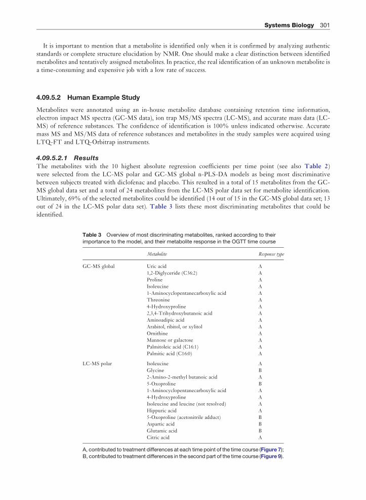
It is important to mention that a metabolite is identified only when it is confirmed by analyzing authenticstandards or complete structure elucidation by NMR. One should make a clear distinction between identifiedmetabolites and tentatively assigned metabolites. In practice, the real identification of an unknown metabolite isa time-consuming and expensive job with a low rate of success.
4.09.5.2 Human Example Study
Metabolites were annotated using an in-house metabolite database containing retention time information,electron impact MS spectra (GC-MS data), ion trap MS/MS spectra (LC-MS), and accurate mass data (LC-MS) of reference substances. The confidence of identification is 100% unless indicated otherwise. Accuratemass MS and MS/MS data of reference substances and metabolites in the study samples were acquired usingLTQ-FT and LTQ-Orbitrap instruments.
4.09.5.2.1 Results
The metabolites with the 10 highest absolute regression coefficients per time point (see also Table 2)were selected from the LC-MS polar and GC-MS global n-PLS-DA models as being most discriminativebetween subjects treated with diclofenac and placebo. This resulted in a total of 15 metabolites from the GC-MS global data set and a total of 24 metabolites from the LC-MS polar data set for metabolite identification.Ultimately, 69% of the selected metabolites could be identified (14 out of 15 in the GC-MS global data set; 13out of 24 in the LC-MS polar data set). Table 3 lists these most discriminating metabolites that could beidentified.
Table 3 Overview of most discriminating metabolites, ranked according to their
importance to the model, and their metabolite response in the OGTT time course
Metabolite Response type
GC-MS global Uric acid A
1,2-Diglyceride (C36:2) A
Proline A
Isoleucine A
1-Aminocyclopentanecarboxylic acid A
Threonine A
4-Hydroxyproline A
2,3,4-Trihydroxybutanoic acid A
Aminoadipic acid A
Arabitol, ribitol, or xylitol A
Ornithine A
Mannose or galactose A
Palmitoleic acid (C16:1) A
Palmitic acid (C16:0) A
LC-MS polar Isoleucine A
Glycine B
2-Amino-2-methyl butanoic acid A
5-Oxoproline B
1-Aminocyclopentanecarboxylic acid A
4-Hydroxyproline A
Isoleucine and leucine (not resolved) A
Hippuric acid A
5-Oxoproline (acetonitrile adduct) B
Aspartic acid B
Glutamic acid B
Citric acid A
A, contributed to treatment differences at each time point of the time course (Figure 7);
B, contributed to treatment differences in the second part of the time course (Figure 9).
Systems Biology 301

4.09.6 Interpretation and Visualization
The transformation from statistical results derived from metabolomics data into biological knowledge is still inits infancy. Many bioinformatics strategies dealing with transcriptomics data have been reported in theliterature. However, tools for the biological interpretation of metabolomics data are scarce at the moment.Pathway tools such as Pathvisio (open source, see www.pathvisio.org) and biological network tools such asMetacore (GeneGo Inc., St. Joseph, MI, USA) and IPA (Ingenuity Systems, Redwood City, CA, USA) provide afirst attempt to connect these components but are not (yet) up to the task. Several challenges have to be facedwhen translating metabolomics results into biology. First of all, metabolomics data in human nutritional studiesare often generated in plasma and urine matrices. The existing pathway and biological network tools deal withintracellular pathways and processes, but this cannot be directly translated into biology of the biofluids thatrepresents whole body metabolism. The ‘intrinsic’ biological function of glucose, for example, is as an energysource, whereas increased glucose concentrations in urine are an indicator for diabetes and increased concen-trations in plasma might be related to the postprandial state and/or insulin (in)sensitivity. Many othermetabolites have less known or more complex functions. Intraorgan concentrations have different relevance,and even intracellular compartmentalization plays a role. The HMDB database (http://www.hmdb.ca/)provides a treasure of information on metabolite properties. NuGOwiki (http://www.nugowiki.org/) poten-tially adds to this knowledge base.
Furthermore, it is not possible to simply compare metabolic organ changes with plasma changes. The bodystrives to maintain homeostasis, and organs need to work hard to keep plasma concentrations betweenacceptable boundaries, thereby showing much more fluctuation than for example in the liver. Inverse correla-tions may even be observed: Oxidative stress produces a sharp drop of glutathione (GSH) in the liver but owingto liver damage, leaking of GSH may increase its concentration in plasma. Urine functions as an accumulatingwaste basket of exogenous compounds and their metabolites, whereas plasma levels of these compounds need tobe as low as possible. So, translation is not straightforward. Statistical relationships between various compart-ments should therefore be treated with care.
Another important concern is the interactions between gut flora and host metabolism. The large-bowelmicroflora produces metabolic signals that might overwhelm the true metabolic signals of nutrients inhuman biofluids.92,93 Furthermore, food will be metabolized in macronutrients that are partly equal toendogenous metabolites. Nutritional researchers like to understand the effects of nutrition on endogenousmetabolic regulation and their impact on health. How to separate the exogenous from endogenousmetabolomes? Metabolomics reveals both, which complicates the interpretation. It is already shown forinstance that consumption of different diets leads to different metabolic profiles in different populations;increases of specific metabolites could be correlated to a high-meat, vegetarian, Atkins, or high-fish diet.94
It is also shown that the metabolic variability remains under the consumption of a standard diet.A reduction in interindividual variation was observed only in urine after a short-time consumption ofstandard diet and not in plasma or saliva.95 Moreover, it will not be simple to understand the separateeffects of age, gender, physical activity, stress, drugs, region, etc. Clearly, significant effort is requiredbefore results from chemometrics can straightforwardly be translated into biological knowledge.Nevertheless, to make nutritional metabolomics or systems biology a real success, biological understandingof the changes detected is crucial.
4.09.6.1 Human Example Study
Only identified metabolites were used for further interpretation of the statistical analysis. Detailedpathway and biological network analysis was performed in Metacore version 4.3 (GeneGo Inc., St.Joseph, MI, USA). Only curated interactions were used for biological network analysis. The followingmetabolites were not available in Metacore and therefore not used for pathway and network analysis:1,2-diglyceride (C36:2), 2,3,4-trihydroxybutanoic acid, and 2-amino-2-methyl butanoic acid, 1-aminocy-clopentanecarboxylic acid. Pathway maps were edited in Mapeditor (GeneGo Inc., St. Joseph, MI, USA)version 2.1.0.
302 Systems Biology

4.09.6.1.1 General interpretation
Most of the selected metabolites (81%, Table 3) showed a difference in offset that is constant during theOGTT time course (Figure 7, response type A). In other words, these metabolites are discriminatingbetween the treated and untreated subjects independent of time during the OGTT time course. Thisindicates that only minor differences exist between the treatment groups, which can be identified only byrepeated measurements. Indeed, time-independent PLS-DA analysis yielded a similar error rate (11%).Several amino acids (n¼ 6), organic acids (n¼ 7), carbohydrates (n¼ 2), and fatty acids and lipids (n¼ 3)were categorized with a response type A. The majority of the response type A metabolites showed adecreased concentration in plasma in response to diclofenac treatment compared to subjects treated withplacebo (results not shown).
Some of the selected metabolites (19%) showed contribution to treatment differences only in the second partof the OGTT time course (Figure 9, response type B). This indicates that these four metabolites differedbetween treatments only when challenging the metabolic situation, leading to alterations in dynamic responseto the perturbation. Indeed, time-independent PLS-DA analysis increased the error rate of the LC-MS polarmodel (26%). The amino acids glycine, aspartic acid, and glutamic acid and the organic acid 5-oxoproline werecategorized with a response type B. All response type B metabolites showed higher concentrations in thediclofenac-treated group.
Some metabolites were identified as being discriminating between the treatments in data from bothanalytical platforms (isoleucine, 1-aminocyclopentanecarboxylic acid, and 4-hydroxyproline), validatingtheir contribution to the differences between the treatment groups.
4.09.6.1.2 Detailed pathway and biological network analysis
Detailed pathway and network analysis identified the modes of action of diclofenac (Figure 12(a)). Diclofenac isknown to inhibit and activate several enzymes and transporters.96–104 The inhibition of the enzyme aminopepti-dase N (CD13) by diclofenac might explain the lower plasma concentrations of the neutral amino acidsL-isoleucine, L-threonine, and L-leucine. CD13 is a broad-specificity aminopeptidase that cleaves specificallythe N-terminal bound neutral amino acids from oligopeptides. Also most of the other neutral amino acidsmeasured showed a lower plasma concentration in diclofenac-treated subjects (L-valine, L-serine, L-cysteine,L-phenylalanine, L-tyrosine, and L-tryptophan, but not L-alanine and L-methionine), whereas most of the basic oracidic plasma amino acids (L-aspartic acid, L-glutamic acid, L-asparagine, and L-histidine) did not show thisconcentration difference (exception is L-lysine). This further confirms that inhibition of CD13 might explain thedifferences found in plasma amino-acid concentrations between the treatment groups. Besides its role in thedigestion of peptides, CD13 is also known to significantly suppress inflammatory immune responses.105,106
Furthermore, diclofenac is known to increase the concentration of kynurenic acid, an endogenous antagonist ofthe N-methyl-D-aspartate receptor (NMDA receptor), having therefore analgesic properties.107,108 The NMDAreceptor is a glutamate receptor, which requires binding of glutamate, aspartate, and the coagonist glycine derivedfrom blood for its efficient opening.105 The NMDA receptor is activated by insulin.109 This might explain theconcentration differences of the amino acids L-glutamate, L-aspartate, and L-glycine that develop at 90–120 minafter glucose intake (metabolites with response type B). Insulin activates the NMDA receptor of placebo-treatedsubjects in response to glucose intake, whereas the NMDA receptor of diclofenac-treated subjects will beinsensitive to insulin because of the increased levels of the antagonist kynurenic acid (Figure 12(b)).
Besides the identification of metabolite changes likely caused by the modes of action of diclofenac,metabolite changes could be identified that were associated with metabolic effects caused by modulation ofthe inflammatory status. Elevated serum uric acid levels are associated with metabolic syndrome, insulinresistance, and type 2 diabetes.110,111 Figure 12(c) presents an overview of the modes of action of uric acid andits relation to glucose metabolism and inflammation. Uric acid inhibits endothelial nitric oxide bioavailability,which is required for insulin to stimulate glucose uptake in cells. Besides its role in the development of insulinresistance, elevated levels of uric acid are associated with inflammation, as serum uric acid has been suggestedas a sensitive marker for vascular inflammation.110–112 The diclofenac treatment resulted in lower levels of uricacid, suggesting that vascular inflammation might be lowered, contributing to increased insulin sensitivity inthese subjects.
Systems Biology 303

Finally, L-5-oxoproline (pyroglutamic acid) is an intermediate of GSH synthesis via the intracellular�-glutamylcysteine cycle. Figure 12(d) presents an overview of the GSH synthesis pathway and its relationto glucose and insulin. Higher clearance of plasma L-5-oxoproline represents a lower GSH synthesis.113 GSHsynthesis is predominantly regulated by the activity of �-glutamylcysteine synthetase (�-GCS). Interestingly,insulin increases and glucose decreases the regulation of GSH synthesis by GCS.114–116 In the current study, thecontrol group showed a clear decrease of 5-oxoproline concentration at 120 min after glucose intake, whereas5-oxoproline concentration in the diclofenac-treated group remained at similar levels compared to previoustime points (response type B metabolite). GSH, measured with the LC-MS polar platform, showed a similardynamic response to glucose as 5-oxoproline. This indicates that diclofenac treatment resulted in a higher GSHsynthesis response after the glucose bolus compared to placebo, suggesting improved insulin sensitivity indiclofenac-treated subjects.
304 Systems Biology
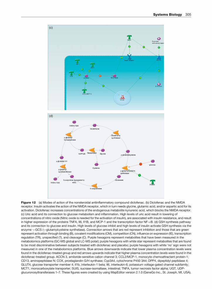
(c)
(d)
Figure 12 (a) Modes of action of the nonsteroidal antiinflammatory compound diclofenac. (b) Diclofenac and the NMDAreceptor. Insulin activates the action of the NMDA receptor, which in turn needs glycine, glutamic acid, and/or aspartic acid for its
activation. Diclofenac increases concentrations of the endogenous metabolite kynurenic acid, which blocks the NMDA receptor.
(c) Uric acid and its connection to glucose metabolism and inflammation. High levels of uric acid result in lowering of
concentrations of nitric oxide (Nitric oxide is needed for the activation of insulin), are associated with insulin resistance, and resultin higher expression of the proteins TNFA, Il6, Il1B, and MCP-1 and the transcription factor NF-�B. (d) GSH synthesis pathway
and its connection to glucose and insulin. High levels of glucose inhibit and high levels of insulin activate GSH synthesis via the
enzyme �-GCS (�-glutamylcysteine synthetase). Connection arrows that are red represent inhibition and those that are greenrepresent activation through binding (B), covalent modifications (CM), competition (CN), influence on expression (IE), transcription
regulation (TR), unspecified (?), and cleavage (C). Purple hexagons represent metabolites that have been measured in the
metabolomics platforms (GC-MS global and LC-MS polar); purple hexagons with white star represent metabolites that are found
to be most discriminative between subjects treated with diclofenac and placebo; purple hexagons with white ‘no’ sign were notmeasured in one of the metabolomics platforms. Blue arrows downwards indicate that lower plasma concentration levels were
found in the diclofenac-treated group and red arrows upwards indicate that higher plasma concentration levels were found in the
diclofenac-treated group. ACCN 3, amiloride-sensitive cation channel 3; CCL2/MCP-1, monocyte chemoattractant protein-1;
CD13, aminopeptidase N; COX, prostaglandin G/H synthase; Cyp3A4, cytochrome P450 3A4; DPP4, dipeptidyl peptidase 4;GLUT4, glucose transporter member 4; Il1b, interleukin-1 beta; Il6, interleukin-6; potassium voltage-gated channel subfamily;
MCT1, monocarboxylate transporter; SUIS, sucrase-isomaltase, intestinal; TNFA, tumor necrosis factor alpha; UGT, UDP-
glucuronosyltransferases 1–7. These figures were created by using MapEditor version 2.1.0 (GeneGo Inc., St. Joseph, MI, USA).
Systems Biology 305

References
1. Ideker, T.; Galitski, T.; Hood, L. A New Approach to Decoding Life: Systems Biology. Annu. Rev. Genomics Hum. Genet. 2001, 2,343–372.
2. Kitano, H. Systems Biology: A Brief Overview. Science 2002, 295, 1662–1664.3. Westerhoff, H. V.; Palsson, B. O. The Evolution of Molecular Biology into Systems Biology. Nat. Biotechnol. 2004, 22, 1249–1252.4. Kritikou, E.; Pulverer, B.; Heinrichs, A. All Systems Go! Suppl. Nat. Rev. Mol. Cell Biol. 2006, 7, 801.5. Bruggeman, F. J.; Westerhoff, H. V. The Nature of Systems Biology. Trends Microbiol. 2007, 15, 45–50.6. Van Der Greef, J.; Smilde, A. K. Symbiosis of Chemometrics and Metabolomics: Past, Present, and Future. J. Chemom. 2005, 19,
376–386.7. Van Ommen, B. Nutrigenomics: Exploiting Systems Biology in the Nutrition and Health Arenas. Nutrition 2004, 20, 4–8.8. Naylor, S.; Culbertson, A. W.; Valentine, S. J. Towards a Systems Level Analysis of Health and Nutrition. Curr. Opin. Biotechnol.
2008, 19, 100–109.9. Kussmann, M.; Rezzi, S.; Daniel, H. Profiling Techniques in Nutrition and Health Research. Curr. Opin. Biotechnol. 2008, 19,
83–99.10. Zhang, X.; Yap, Y.; Wei, D.; Chen, G.; Chen, F. Novel Omics Technologies in Nutrition Research. Biotechnol. Adv. 2008, 26,
169–176.11. Afman, L.; Muller, M. Nutrigenomics: From Molecular Nutrition to Prevention of Disease. J. Am. Diet. Assoc. 2006, 106, 569–576.12. Chavez, A.; Munoz de Chavez, M. Nutrigenomics in Public Health Nutrition: Short-Term Perspectives. Eur. J. Clin. Nutr. 2003, 57,
S97–S100.13. Muller, M.; Kersten, S. Nutrigenomics: Goals and Strategies. Nat. Rev. Genet. 2003, 4, 315–322.14. Watkins, S. M.; Hammock, B. D.; Newman, J. W.; German, J. B. Individual Metabolism Should Guide Agriculture toward Foods
for Improved Health and Nutrition. Am. J. Clin. Nutr. 2001, 74 (3), 283–286.15. Gibney, M. J.; Walsh, M.; Brennan, L.; Roche, H. M.; German, B.; Van Ommen, B. Metabolomics in Human Nutrition:
Opportunities and Challenges. Am. J. Clin. Nutr. 2005, 82, 497–503.16. Horgan, G. W. Sample Size and Replication in 2D Gel Electrophoresis Studies. J. Proteome Res. 2007, 6 (7), 2884–2887.17. Guo, X.; Johnson, W. D. Sample Sizes for Experiments with Multivariate Repeated Measures. J. Biopharm. Stat. 1996, 6 (2),
155–176.18. Storey, J. D.; Tibshirani, R. Statistical Methods for Identifying Differentially Expressed Genes in DNA Microarrays. Methods Mol.
Biol. 2003, 224, 149–157.19. Tibshirani, R. A Simple Method for Assessing Sample Sizes in Microarray Experiments. BMC Bioinf. 2006, 7, 106.20. Ferreira, J. A.; Zwinderman, A. Approximate Sample Size Calculations with Microarray Data: An Illustration. Stat. Appl. Genet.
Mol. Biol. 2006, 5, 25.21. Rubingh, C. M.; Van Erk, M. J.; Wopereis, S.; Van Vliet, T.; Verheij, E. R.; Cnubben, N. H. P.; Van Ommen, B.; Van Der Greef, J.;
Hendriks, H. F. J.; Smilde, A. K. Discovery of Subtle Effects in a Human Intervention Trial through Multilevel Modeling. Submittedto BMC Bioinformatics.
22. Wopereis, S.; Rubingh, C. M.; Van Erk, M. J.; Verheij, E. R.; Van Vliet, T.; Cnubben, N. H. P.; Smilde, A. K.; Van Der Greef, J.; VanOmmen, B.; Hendriks, H. F. J. A Metabolic Profiling of the Response to an Oral Glucose Tolerance Test Detects Subtle MetabolicChanges. Accepted for publication by PLoS ONE.
23. Eddy, D. M.; Schlessinger, L.; Kahn, R. Clinical Outcomes and Cost-Effectiveness of Strategies for Managing People at High Riskfor Diabetes. Ann. Intern. Med. 2005, 143, 251–264.
24. Goldstein, D. E.; Little, R. R.; Lorenz, R. A.; Malone, J. I.; Nathan, D.; Peterson, C. M.; Sacks, D. B. Tests of Glycemia in Diabetes.Diabetes Care 2004, 27, 1761–1773.
25. Stumvoll, M.; Goldstein, B. J.; Van Haeften, T. W. Type 2 Diabetes: Principles of Pathogenesis and Therapy. Lancet 2005, 365,1333–1346.
26. Teahan, O.; Gamble, S.; Holmes, E.; Waxman, J.; Nicholson, J. K.; Bevan, C.; Keun, H. C. Impact of Analytical Bias inMetabonomic Studies of Human Blood Serum and Plasma. Anal. Chem. 2006, 78, 4307–4318.
27. Lauridsen, M.; Hansen, S. H.; Jaroszewski, J. W.; Cornett, C. Human Urine as Test Material in 1H NMR-Based Metabonomics:Recommendations for Sample Preparation and Storage. Anal. Chem. 2007, 79, 1181–1186.
28. Gika, H. G.; Theodoridis, G. A.; Wilson, I. D. Liquid Chromatography and Ultra-Performance Liquid Chromatography-MassSpectrometry Fingerprinting of Human Urine. Sample Stability under Different Handling and Storage Conditions forMetabonomics Studies. J. Chromatogr. A 2008, 1189, 314–322.
29. Lindon, J. C.; Nicholson, J. K.; Holmes, E., Eds.; The Handbook of Metabonomics and Metabolomics. Elsevier Science:Amsterdam, 2007.
30. Kolokolova, T. N.; Savel’ev, O. Y.; Sergeev, N. M. Metabolic Analysis of Human Biological Fluids by 1H NMR Spectroscopy.J. Anal. Chem. 2008, 63 (2), 104–120.
31. Gika, H. G.; Theodoridis, G. A.; Wingate, J. E.; Wilson, I. D. Within-Day Reproducibility of an HPLC-MS-Based Method forMetabonomic Analysis: Application to Human Urine. J. Proteome Res. 2007, 6, 3291–3303.
32. Sangster, T.; Major, H.; Plumb, R.; Wilson, A. J.; Wilson, I. D. A Pragmatic and Readily Implemented Quality Control Strategy forHPLC-MS and GC-MS-Based Metabolomic Analysis. Analyst 2006, 131, 1075–1078.
33. Sangster, T.; Wingate, J. E.; Burton, L.; Teichert, F.; Wilson, I. D. Investigation of Analytical Variation in Metabonomic AnalysisUsing Liquid Chromatography/Mass Spectrometry. Rapid Commun. Mass Spectrom. 2007, 21, 2965–2970.
34. Wilson, I. D.; Plumb, R.; Granger, J.; Major, H.; Williams, R.; Lenz, E. M. Review: HPLC-MS-Based Methods for the Study ofMetabonomics. J. Chromatogr. B 2005, 817, 67–76.
35. Koek, M. M.; Muilwijk, B.; Van Der Werf, M. J.; Hankemeier, Th. Microbial Metabolomics with Gas Chromatography/MassSpectrometry. Anal. Chem. 2006, 78, 1272–1281.
36. Fiehn, O. Extending the Breadth of Metabolite Profiling by Gas Chromatography Coupled to Mass Spectrometry. Trends Anal.Chem. 2008, 27 (3), 261–269.
306 Systems Biology

37. Dunn, W. B.; Ellis, D. I. Metabolomics: Current Analytical Platforms and Methodologies. Trends Anal. Chem. 2005, 24 (4), 285–294.38. Hollywood, K.; Brison, D. R.; Goodacre, R. Metabolomics: Current Technologies and Future Trends. Proteomics 2006, 6,
4716–4723.39. Want, E. J.; Nordstrom, A.; Morita, H.; Siuzdak, G. From Exogenous to Endogenous: The Inevitable Imprint of Mass Spectrometry
in Metabolomics. J. Proteome Res. 2007, 6, 459–468.40. Lindon, J. C.; Nicholson, J. K. Analytical Technologies for Metabonomics and Metabolomics, and Multi-Omic Information
Recovery. Trends Anal. Chem. 2007, 27 (3), 194–204.41. Dettmer, K.; Aronov, P. A.; Hammock, B. D. Mass Spectrometry-Based Metabolomics. Mass Spectrom. Rev. 2007, 26, 51–78.42. Lenz, E. M.; Wilson, I. D. Analytical Strategies in Metabonomics. J. Proteome Res. 2007, 6, 443–458.43. Roberston, D. G.; Reily, M. D.; Baker, J. D. Metabonomics in Pharmaceutical Discovery and Development. J. Proteome Res.
2007, 6, 526–539.44. Issaq, H. J.; Abbott, E.; Veenstra, T. D. Utility of Separation Science in Metabolomic Studies. J. Sep. Sci. 2008, 31, 1936–1947.45. Theodoridis, G.; Gika, H. G.; Wilson, I. D. LC-MS-Based Methodology for Global Metabolite Profiling in Metabonomics/
Metabolomics. Trends Anal. Chem. 2008, 27 (3), 251–260.46. Lu, X.; Zhao, X.; Bai, C.; Zhao, C.; Lu, G.; Xu, G. Review: LC-MS-Based Metabonomics Analysis. J. Chromatogr. B 2008, 866,
64–76.47. Bedair, M.; Sumner, L. W. Current and Emerging Mass-Spectrometry Technologies for Metabolomics. Trends Anal. Chem. 2008,
27 (3), 238–250.48. Van Der Greef, J.; Martin, S.; Juhasz, P.; Adourian, A.; Plasterer, T.; Verheij, E. R.; McBurney, R. N. The Art and Practice of
Systems Biology in Medicine: Mapping Patterns of Relationships. J. Proteome Res. 2007, 6, 1540–1559.49. van der Werf, M. J.; Overkamp, K. M.; Muilwijk, B.; Coulier, L.; Hankemeier, Th. Microbial Metabolomics: Toward a Platform with
Full Metabolome Coverage. Anal. Biochem. 2007, 370, 17–25.50. Kind, T.; Tolstikov, V.; Fiehn, O.; Weiss, R. H. A Comprehensive Urinary Metabolomic Approach for Identifying Kidney Cancer.
Anal. Biochem. 2007, 363, 185–195.51. Lawton, K. A.; Berger, A.; Mitchell, M.; Milgram, K. E.; Evans, A. M.; Guo, L.; Hanson, R. W.; Kalhan, S. C.; Ryals, J. A.; Milburn,
M. V. Analysis of the Adult Human Plasma Metabolome. Pharmacogenomics 2008, 9 (4), 383–397.52. Williams, R.; Lenz, E. M.; Wilson, A. J.; Granger, J.; Wilson, I. D.; Major, H.; Stumpf, C.; Plumb, R. A Multi-Analytical Platform
Approach to the Metabonomic Analysis of Plasma from Normal and Zucker (fa/fa) Obese Rats. Mol. Biosyst. 2006, 2, 174–183.53. Kaddurah-Daouk, R.; Kristal, B. S.; Weinshilboum, R. M. Metabolomics: A Global Biochemical Approach to Drug Response and
Disease. Annu. Rev. Pharmacol. Toxicol. 2008, 48, 653–683.54. Van der Greef, J.; Hankemeier, Th.; McBurney, R. N. Metabolomics-Based Systems Biology and Personalized Medicine: Moving
Towards n¼ 1 Clinical Trials? Pharmacogenomics 2006, 7, 1087–1094.55. Bijlsma, S.; Bobeldijk, I.; Verheij, E. R.; Ramaker, R.; Kochhar, S.; MacDonald, I. A.; Van Ommen, B.; Smilde, A. K. Large-Scale
Human Metabolomics Studies: A Strategy for Data (Pre-)Processing and Validation. Anal. Chem. 2006, 78, 567–574.56. Newman, J. W.; Kaysen, G. A.; Hammock, B. D.; Shearer, G. C. Proteinuria Increases Oxylipid Concentrations in VLDL and HDL
but not LDL Particles in the Rat. J. Lipid Res. 2007, 48, 1792–1800.57. Maeda, Y.; Ito, T.; Suzuki, A.; Kurono, Y.; Ueta, A.; Yokoi, K.; Sumi, S.; Togari, H.; Sugiyama, N. Simultaneous Quantification of
Acylcarnitine Isomers Containing Dicarboxylic Acylcarnitines in Human Serum and Urine by High-Performance LiquidChromatography/Electrospray Ionization Tandem Mass Spectrometry. Rapid Commun. Mass Spectrom. 2007, 21, 799–806.
58. Ammann, A. A. Inductively Coupled Plasma Mass Spectrometry (ICP MS): A Versatile Tool. J. Mass Spectrom. 2007, 42, 419–427.59. Kingsley, P. J.; Marnett, L. J. LC-MS-MS Analysis of Neutral Eicosanoids. Methods Enzymol. 2007, 433, 91–112.60. Lau, H. L.; Puah, C. W.; Choo, Y. M.; Ma, A. N.; Chuah, C. H. Simultaneous Quantification of Free Fatty Acids, Free Sterols,
Squalene, and Acylglycerol Molecular Species in Palm Oil by High-Temperature Gas Chromatography-Flame IonizationDetection. Lipids 2005, 40, 523–528.
61. Kristal, B. S.; Shurubor, Y. I.; Kaddurah-Daouk, R.; Matson, W. R. High-Performance Liquid Chromatography Separations Coupledwith Coulometric Electrode Array Detectors: A Unique Approach to Metabolomics. Methods Mol. Biol. 2007, 358, 159–174.
62. Pham-Tuan, H.; Kaskavelis, L.; Daykin, C. A.; Janssen, H. G. Method Development in High-Performance Liquid Chromatographyfor High-Throughput Profiling and Metabonomic Studies of Biofluid Samples. J. Chromatogr. B Analyt. Technol. Biomed. Life Sci.2003, 789, 283–301.
63. Bruce, S. J.; Jonsson, P.; Antti, H.; Cloarec, O.; Trygg, J.; Marklund, S. L.; Moritz, T. Evaluation of a Protocol for MetabolicProfiling Studies on Human Blood Plasma by Combined Ultra-Performance Liquid Chromatography/Mass Spectrometry: FromExtraction to Data Analysis. Anal. Biochem. 2008, 372, 237–249.
64. Verhoeckx, K. C. M.; Bijlsma, S.; Jespersen, S.; Ramaker, R.; Verheij, E. R.; Witkamp, R. F.; Van der Greef, J.; Rodenburg, R. J. T.Characterization of Anti-Inflammatory Compounds Using Transcriptomics, Proteomics, and Metabolomics in Combination withMultivariate Data Analysis. Int. Immunopharmacol. 2004, 4, 1499–1514.
65. Walczak, B.; Wu, W. Fuzzy Warping of Chromatograms. Chemom. Intell. Lab. Syst. 2005, 77, 173–180.66. Windig, W.; Smith, W. F. Chemometric Analysis of Complex Hyphenated Data: Improvements of the Component Detection
Algorithm. J. Chromatogr. A 2007, 1158, 251–257.67. Van Der Greef, J.; Vogels, J. T. W. E.; Wulfert, F.; Tas, A. C. Method and System for Identifying and Quantifying Chemical
Components of a Mixture. U.S. Patent 2,004,267,459, 2004.68. Clish, C. B.; Davidov, E.; Oresic, M.; Plasterer, T. N.; Lavine, G.; Londo, T.; Adourian, A.; Zhang, X.; Johnston, M.; Morel, N.;
Marple, E. W.; Plasterer, T. N.; Neumann, E.; Verheij, E.; Vogels, J. T. W. E.; Havekes, L. M.; Van der Greef, J.; Naylor, S.Integrative Biological Analysis of the APOE�3-Leiden Transgenic Mouse. OMICS 2004, 8, 3–13.
69. Van Der Greef, J.; Van Der Heijden, R.; Verheij, E. R. The Role of Mass Spectrometry in Systems Biology: Data Processing andIdentification Strategies in Metabolomics. In Advances in Mass Spectrometry; Ashcroft, A. E., Brenton, G., Monaghen, J. J., Eds.;Elsevier Science: Amsterdam, 2004; pp 145–165.
70. Smilde, A. K.; van der Werf, M. J.; Bijlsma, S.; van Der Werff-van Der Vat, B. J.; Jellema, R. H. Fusion of Mass Spectrometry-Based Metabolomics Data. Anal. Chem. 2005, 77, 6729–6736.
Systems Biology 307

71. Smilde, A. K.; Bro, R.; Geladi, P. Multi-Way Analysis. Applications in the Chemical Sciences; John Wiley & Sons: Chichester,2004.
72. Kiers, H. A. L.; Mechelen, I. Three-Way Component Analysis: Principles and Illustrative Application. Psychol. Methods 2001, 6,84–110.
73. Harshman, R. A.; Lundy, M. E. PARAFAC: Parallel Factor Analysis. Comput. Stat. Data Anal. 1994, 18, 39–72.74. Westerhuis, J. A.; Derks, E. P. P. A.; Hoefsloot, H. C.; Smilde, A. K. Grey Component Analysis. J. Chemom. 2007, 21,
474–485.75. Bang, J.-W.; Crockford, D. J.; Holmes, E.; Pazos, F.; Sternberg, M. J. E.; Muggleton, S. H.; Nicholson, J. K. Integrative Top-Down
System Metabolic Modeling in Experimental Disease States via Data-Driven Bayesian Methods. J. Proteome Res. 2008, 1,497–503.
76. Stone, M. Cross-Validatory Choice and Assessment of Statistical Predictions. J. R. Stat. Soc. Ser. B 1974, 36, 111–147.77. Smit, S.; Van Breemen, M. J.; Hoefsloot, H. C. J.; Smilde, A. K.; Aerts, J. M. F. G.; De Koster, C. G. Assessing the Statistical
Validity of Proteomics Based Biomarkers. Anal. Chim. Acta 2007, 592, 210–217.78. Zamboni, N.; Kummel, A.; Heinemann, M. AnNET: A Tool for Network-Embedded Thermodynamic Analysis of Quantitative
Metabolome Data. BMC Bioinf. 2008, 9, 199.79. Barker, M.; Rayens, W. Partial Least Squares for Discrimination. J. Chemom. 2003, 17, 166–173.80. Van Velzen, E. J. J.; Westerhuis, J. A.; Van Duynhoven, J. P. M.; Van Dorsten, F. A.; Hoefsloot, H. C. J.; Smit, S.; Draijer, R.;
Kroner, C. I.; Smilde, A. K. Multilevel Data Analysis of a Crossover-Design Human Nutritional Study. J. Proteome Res. 2008, 7,4483–4491.
81. Bro, R. Multiway Calibration. Multilinear PLS. J. Chemom. 1996, 10, 47–61.82. Smilde, A. K. Comments on Multilinear PLS. J. Chemom. 1997, 11, 367–377.83. Smilde, A. K.; Bro, R.; Geladi, P. Multi-Way Analysis: Applications in the Chemical Sciences; John Wiley & Sons: West Sussex, 2004;
pp 221–256.84. Martens, H.; Naes, T. Multivariate Calibration; John Wiley & Sons: Chichester, 1989.85. Andersson, C. A.; Bro, R. The N-Way Toolbox for MATLAB. Chemom. Intell. Lab. Syst. 2000, 52, 1–4.86. Wishart, D. S.; Tzur, D.; Knox, C.; Eisner, R.; Guo, A. C.; Young, N.; Cheng, D.; Jewell, K.; Arndt, D.; Sawhney, S.; Fung, C.;
Nikolai, L.; Lewis, M.; Coutouly, M.-A.; Forsythe, I.; Tang, P.; Shrivastava, S.; Jeroncic, K.; Stothard, P.; Amegbey, G.; Block, D.;Hau, D. D.; Wagner, J.; Miniaci, J.; Clements, M.; Gebremedhin, M.; Guo, N.; Zhang, Y.; Duggan, G. E.; MacInnis, G. D.; Weljie,A. M.; Dowlatabadi, R.; Bamforth, F.; Clive, D.; Greiner, R.; Li, L.; Marrie, T.; Sykes, B. D.; Vogel, H. J.; Querengesser, L. HMDB:The Human Metabolome Database. Nucleic Acids Res. 2007, 35, D521–D526.
87. Wishart, D. S. Human Metabolome Database: Completing the ‘Human Parts List’. Pharmacogenomics 2007, 8, 683–686.88. Kopka, J. Current Challenges and Developments in GC-MS Based Metabolite Profiling Technology. J. Biotechnol. 2006, 124,
312–322.89. Lindon, J. C.; Nicholson, J. K.; Wilson, I. D. Directly Coupled HPLC-NMR and HPLC-NMR-MS in Pharmaceutical Research and
Development. J. Chromatogr. B 2000, 748, 233–258.90. Kind, T.; Fiehn, O. Metabolomic Database Annotations via Query of Elemental Compositions: Mass Accuracy Is Insufficient Even
at Less than 1 ppm. BMC Bioinf. 2006, 7, 234.91. Kind, T.; Fiehn, O. Seven Golden Rules for Heuristic Filtering of Molecular Formulas Obtained by Accurate Mass Spectrometry.
BMC Bioinf. 2007, 8, 105.92. Goodacre, R. Metabolomics of a Superorganism. J. Nutr. 2007, 137, 259S–266S.93. Dumas, M. E.; Barton, R. H.; Toye, A.; Cloarec, O.; Blancher, C.; Rothwell, A.; Fearnside, J.; Tatoud, R.; Blanc, V.; Lindon,
J. C.; Mitchell, S. C.; Holmes, E.; McCarthy, M. I.; Scott, J.; Gauguier, D.; Nicholson, J. K. Metabolic Profiling Reveals aContribution of Gut Microbiota to Fatty Liver Phenotype in Insulin-Resistant Mice. Proc. Natl. Acad. Sci. U.S.A. 2006, 103,12511–12516.
94. Rezzi, S.; Ramadan, Z.; Fay, L. B.; Kochhar, S. Nutritional Metabonomics: Applications and Perspectives. J. Proteome Res. 2007,6, 513–525.
95. Walsh, M. C.; Brennan, L.; Malthouse, J. P.; Roche, H. M.; Gibney, M. J. Effect of Acute Dietary Standardization on the Urinary,Plasma, and Salivary Metabolomic Profiles of Healthy Humans. Am. J. Clin. Nutr. 2006, 84, 531–539.
96. Boelsterli, U. A. Diclofenac-Induced Liver Injury: A Paradigm of Idiosyncratic Drug Toxicity. Toxicol. Appl. Pharmacol. 2003, 192,307–322.
97. Choi, J. S.; Jin, M. J.; Han, H. K. Role of Monocarboxylic Acid Transporters in the Cellular Uptake of NSAIDs. J. Pharm.Pharmacol. 2005, 57, 1185–1189.
98. Mano, Y.; Usui, T.; Kamimura, H. In Vitro Inhibitory Effects of Non-Steroidal Antiinflammatory Drugs on UDP-Glucuronosyltransferase 1A1-Catalysed Estradiol 3? – Glucuronidation in Human Liver Microsomes. Biopharm. Drug Dispos.2005, 26, 35–39.
99. Masubuchi, Y.; Ose, A.; Horie, T. Diclofenac-Induced Inactivation of CYP3A4 and Its Stimulation by Quinidine. Drug Metab.Dispos. 2002, 30, 1143–1148.
100. Peretz, A.; Degani, N.; Nachman, R.; Uziyel, Y.; Gibor, G.; Shabat, D.; Attali, B. Meclofenamic Acid and Diclofenac, NovelTemplates of KCNQ2/Q3 Potassium Channel Openers, Depress Cortical Neuron Activity and Exhibit Anticonvulsant Properties.Mol. Pharmacol. 2005, 67, 1053–1066.
101. Uchaipichat, V.; Mackenzie, P. I.; Guo, X. H.; Gardner-Stephen, D.; Galetin, A.; Houston, J. B.; Miners, J. O. Human UDP-Glucuronosyltransferases: Isoform Selectivity and Kinetics of 4-Methylumbelliferone and 1-Naphthol Glucuronidation, Effects ofOrganic Solvents, and Inhibition by Diclofenac and Probenecid. Drug Metab. Dispos. 2004, 32, 413–423.
102. Voilley, N.; De Weille, J.; Mamet, J.; Lazdunski, M. Nonsteroid Anti-Inflammatory Drugs Inhibit Both the Activity and theInflammation-Induced Expression of Acid-Sensing Ion Channels in Nociceptors. J. Neurosci. 2001, 21, 8026–8033.
103. Wade, L. T.; Kenna, J. G.; Caldwell, J. Immunochemical Identification of Mouse Hepatic Protein Adducts Derived from theNonsteroidal Anti-Inflammatory Drugs Diclofenac, Sulindac, and Ibuprofen. Chem. Res. Toxicol. 1997, 10, 546–555.
104. Ware, J. A.; Graf, M. L. M.; Martin, B. M.; Lustberg, L. R.; Pohl, L. R. Immunochemical Detection and Identification of ProteinAdducts of Diclofenac in the Small Intestine of Rats: Possible Role in Allergic Reactions. Chem. Res. Toxicol. 1998, 11, 164–171.
308 Systems Biology

105. Chen, P. E.; Geballe, M. T.; Stansfeld, P. J.; Johnston, A. R.; Yuan, H.; Jacob, A. L.; Snyder, J. P.; Traynelis, S. F.; Wyllie, D. J.Structural Features of the Glutamate Binding Site in Recombinant NR1/NR2A N-Methyl-D-Aspartate Receptors Determined bySite-Directed Mutagenesis and Molecular Modeling. Mol. Pharmacol. 2005, 67, 1470–1484.
106. Reinhold, D.; Biton, A.; Goihl, A.; Pieper, S.; Lendeckel, U.; Faust, J.; Neubert, K.; Bank, U.; Ger, M.; Ansorge, S.; Brocke, S. DualInhibition of Dipeptidyl Peptidase IV and Aminopeptidase N Suppresses Inflammatory Immune Responses. Ann. N. Y. Acad.Sci. 2007, 1110, 402–409.
107. Edwards, S. R.; Mather, L. E.; Lin, Y.; Power, I.; Cousins, M. J. Glutamate and Kynurenate in the Rat Central Nervous SystemFollowing Treatments with Tail Ischaemia or Diclofenac. J. Pharm. Pharmacol. 2000, 52, 59–66.
108. Schwieler, L.; Erhardt, S.; Erhardt, C.; Engberg, G. Prostaglandin-Mediated Control of Rat Brain Kynurenic Acid Synthesis –Opposite Actions by COX-1 and COX-2 Isoforms. J. Neural Transm. 2005, 112, 863–872.
109. Liao, G. Y.; Leonard, J. P. Insulin Modulation of Cloned Mouse NMDA Receptor Currents in Xenopus Oocytes. J. Neurochem.1999, 73, 1510–1519.
110. Becker, M. A.; Jolly, M. Hyperuricemia and Associated Diseases. Rheum. Dis. Clin. North Am. 2006, 32, 275–293.111. Hayden, M. R.; Tyagi, S. C. Uric Acid: A New Look at an Old Risk Marker for Cardiovascular Disease, Metabolic Syndrome, and
Type 2 Diabetes Mellitus: The Urate Redox Shuttle. Nutr. Metab. 2004, 1 (1), 10.112. Nakagawa, T.; Hu, H.; Zharikov, S.; Tuttle, K. R.; Short, R. A.; Glushakova, O.; Ouyang, X.; Feig, D. I.; Block, E. R.; Herrera-
Acosta, J.; Patel, J. M.; Johnson, R. J. A Causal Role for Uric Acid in Fructose-Induced Metabolic Syndrome. Am. J. Physiol.Renal Physiol. 2006, 290, F625–F631.
113. Yu, Y. M.; Ryan, C. M.; Fei, Z. W.; Lu, X. M.; Castillo, L.; Schultz, J. T.; Tompkins, R. G.; Young, V. R. Plasma L-5-OxoprolineKinetics and Whole Blood Glutathione Synthesis Rates in Severely Burned Adult Humans. Am. J. Physiol. Endocrinol. Metab.2002, 282, E247–E258.
114. Lu, S. C. Regulation of Glutathione Synthesis. Curr. Top. Cell. Regul. 2000, 36, 95–116.115. Townsend, D. M.; Tew, K. D.; Tapiero, H. The Importance of Glutathione in Human Disease. Biomed. Pharmacother. 2003, 57,
145–155.116. Wu, G.; Fang, Y. Z.; Yang, S.; Lupton, J. R.; Turner, N. D. Glutathione Metabolism and Its Implications for Health. J. Nutr. 2004,
134, 489–492.
Systems Biology 309
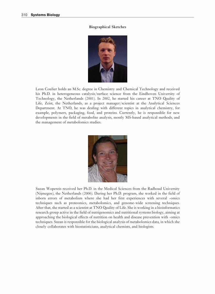
Biographical Sketches
Leon Coulier holds an M.Sc. degree in Chemistry and Chemical Technology and receivedhis Ph.D. in heterogeneous catalysis/surface science from the Eindhoven University ofTechnology, the Netherlands (2001). In 2002, he started his career at TNO Quality ofLife, Zeist, the Netherlands, as a project manager/scientist at the Analytical SciencesDepartment. At TNO, he was dealing with different topics in analytical chemistry, forexample, polymers, packaging, food, and proteins. Currently, he is responsible for newdevelopments in the field of metabolite analysis, mostly MS-based analytical methods, andthe management of metabolomics studies.
Suzan Wopereis received her Ph.D. in the Medical Sciences from the Radboud University(Nijmegen), the Netherlands (2006). During her Ph.D. program, she worked in the field ofinborn errors of metabolism where she had her first experiences with several -omicstechniques such as proteomics, metabolomics, and genome-wide screening techniques.After that, she started as a scientist at TNO Quality of Life. She is working in a bioinformaticsresearch group active in the field of nutrigenomics and nutritional systems biology, aiming atapproaching the biological effects of nutrition on health and disease prevention with -omicstechniques. Suzan is responsible for the biological analysis of metabolomics data, in which sheclosely collaborates with biostatisticians, analytical chemists, and biologists.
310 Systems Biology

Upon her graduation in human nutrition and health at Wageningen University in 1999,Carina Rubingh (1976) started working at TNO Quality of Life, Zeist, The Netherlands. Shereceived her M.Sc. degree in biostatistics in 2004 from the University of Hasselt, Belgium. In2005, while still working at TNO, she started her Ph.D. at the University of Amsterdam, theNetherlands, on the subject of analysis and validation of metabolomics data. Currently, she isworking as a biostatistician in the product group ‘Analytical Information Sciences’, perform-ing both univariate and multivariate statistics. Her main focus is on data analysis ofmetabolomics studies, experimental design, and statistical consultancy.
Henk Hendriks (1957) studied Biology at State University Utrecht and received his Ph.D.from the State University Leiden in 1991. In 1986, he started working at TNO (IVEG,Rijswijk) in the Department of Dementia and Cell Physiology. At present, he is working atTNO Quality of Life in Zeist as a senior project leader – Human Volunteer Studies(Department Biosciences). Henk Hendriks’ special fields of interest are biomedical aspectsof moderate alcohol consumption in man, nutrition and coronary heart disease risk factors,functional food claim support, and novel food safety evaluation.
Systems Biology 311

Marijana Radonjic was born on the 24th of October 1976 in Belgrade (Yugoslavia, Serbia).Upon graduation at The First Belgrade Gymnasium in 1995, she studied Molecular Biologyand Physiology at the University of Belgrade and obtained B.Sc./M.Sc. degree in AppliedBiochemistry in 2001. From 2001 to 2006, she studied genomics approaches in the field ofeukaryotic transcription regulation in the Department of Physiological Chemistry, UtrechtUniversity, the Netherlands. For this research, she received a Ph.D. degree in September2006. Since 2006, Marijana is employed by the Dutch National Institute for Applied Sciences(TNO), Business Unit Biosciences, Department of Physiological Genomics, as a researchscientist responsible for analysis and integration of -omics data in nutritional and toxicolo-gical studies.
Renger Jellema, Ph.D., TNO Quality of Life, has a track record of more than 10 yearsworking in the field of chemometrics. His roots are in analytical chemistry for which heobtained a bachelor degree in 1992. Renger studied chemistry at the University of Nijmegen(Radboud University), which he finished in 1995. Subsequently, he did his Ph.D. at theUniversity of Amsterdam in collaboration with the steel company Corus. After a shortappointment at the Central Bureau of Statistics (CBS), he obtained his current position atTNO Quality of Life, Zeist where he is currently working in the field of chemometrics asProduct Manager of the product group ‘Analytical Information Sciences’. The main topics ofinterest in chemometrics are experimental design, application and development of methodsand tools for data preprocessing, multivariate statistics, and visualization.
312 Systems Biology

Comparative Modeling of Drug Target Proteins☆
B Webb, N Eswar, H Fan, N Khuri, U Pieper, GQ Dong, and A Sali, University of California at San Francisco, San Francisco, CA, USA
ã 2014 Elsevier Inc. All rights reserved.
Introduction 2Structure-Based Drug Discovery 2The Sequence–Structure Gap 2Structure Prediction Addresses the Sequence–Structure Gap 2The Basis of Comparative Modeling 2Comparative Modeling Benefits from Structural Genomics 2Outline 2Steps in Comparative Modeling 3Fold Assignment and Sequence–Structure Alignment 3Fold assignment 3Three levels of similarity 3Sequence–sequence methods 4Sequence–profile methods 4Profile–profile methods 4Sequence–structure threading methods 5Iterative sequence–structure alignment 5Most Alignment Errors are Unrecoverable 5Template Selection 5Model Building 5Three Approaches to Comparative Model Building 5Modeller: Comparative Modeling by Satisfaction of Spatial Restraints 6Relative Accuracy, Flexibility, and Automation 6Refinement of Comparative Models 6Loop Modeling 6Definition of the problem 6Two classes of methods 6Side-Chain Modeling 7Fixed backbone 7Rotamers 7Methods 7Errors in Comparative Models 7Selection of Incorrect Templates 7Errors due to Misalignments 7Errors in Regions without a Template 8Distortions and Shifts in Correctly Aligned Regions 8Errors in Side-Chain Packing 9Prediction of Model Errors 9Initial Assessment of the Fold 9Self-Consistency 9Final Assessment of the Fold (Model) 9Evaluation of Comparative Modeling Methods 9Applications of Comparative Models 10Comparative Models versus Experimental Structures in Virtual Screening 11Use of Comparative Models to Obtain Novel Drug Leads 11Future Directions 12Automation and Availability of Resources for Comparative Modeling and Ligand Docking 13Acknowledgments 15References 16
☆Change History: August 2014. B Webb updated the reference section and brought the entire text up to date.
H Fan updated section ‘Comparative Models versus Experimental Structures in Virtual Screening’ with new studies, and removed the old Figure 5.
N Khuri added new studies to section ‘Use of Comparative Models to Obtain Novel Drug Leads.’
U Pieper updated section ‘Automation and Availability of Resources for Comparative Modeling and Ligand Docking,’ Table 1, and Figure 5.
GQ Dong added a new section ‘Final Assessment of the Fold (Model selection).’
Reference Module in Chemistry, Molecular Sciences and Chemical Engineering http://dx.doi.org/10.1016/B978-0-12-409547-2.11133-3 1

2 Comparative Modeling of Drug Target Proteins
Introduction
Structure-Based Drug Discovery
Structure-based or rational drug discovery has already resulted in a number of drugs on the market and many more in the
development pipeline.1–4 Structure-based methods are now routinely used in almost all stages of drug development, from target
identification to lead optimization.5–8 Central to all structure-based discovery approaches is the knowledge of the three-
dimensional (3D) structure of the target protein or complex because the structure and dynamics of the target determine which
ligands it binds. The 3D structures of the target proteins are best determined by experimental methods that yield solutions at atomic
resolution, such as X-ray crystallography and nuclear magnetic resonance (NMR) spectroscopy.9 While developments in the
techniques of experimental structure determination have enhanced the applicability, accuracy, and speed of these structural
studies,10,11 structural characterization of sequences remains an expensive and time-consuming task.
The Sequence–Structure Gap
The publicly available Protein Data Bank (PDB)12 currently contains �92 000 structures and grows at a rate of approximately 40%
every 2 years. On the other hand, the various genome-sequencing projects have resulted in over 40million sequences, including the
complete genetic blueprints of humans and hundreds of other organisms.13,14 This achievement has resulted in a vast collection of
sequence information about possible target proteins with little or no structural information. Current statistics show that the
structures available in the PDB account for less than 1% of the sequences in the UniProt database.13 Moreover, the rate of growth of
the sequence information is more than twice that of the structures, and is expected to accelerate even more with the advent of
readily available next-generation sequencing technologies. Due to this wide sequence–structure gap, reliance on experimentally
determined structures limits the number of proteins that can be targeted by structure-based drug discovery.
Structure Prediction Addresses the Sequence–Structure Gap
Fortunately, domains in protein sequences are gradually evolving entities that can be clustered into a relatively small number of
families with similar sequences and structures.15,16 For instance, 75–80% of the sequences in the UniProt database have been
grouped into fewer than 15 000 domain families.17,18 Similarly, all the structures in the PDB have been classified into about 1000
distinct folds.19,20 Computational protein structure prediction methods, such as threading21 and comparative protein structure
modeling,22,23 strive to bridge the sequence–structure gap by utilizing these evolutionary relationships. The speed, low cost, and
relative accuracy of these computational methods have led to the use of predicted 3D structures in the drug discovery process.24,25
The other class of prediction methods, de novo or ab initiomethods, attempts to predict the structure from sequence alone, without
reliance on evolutionary relationships. However, despite progress in these methods,26–28 especially for small proteins with fewer
than 100 amino acid residues, comparative modeling remains the most reliable method of predicting the 3D structure of a protein,
with an accuracy that can be comparable to a low-resolution, experimentally determined structure.9
The Basis of Comparative Modeling
The primary requirement for reliable comparative modeling is a detectable similarity between the sequence of interest (target
sequence) and a known structure (template). As early as 1986, Chothia and Lesk29 showed that there is a strong correlation
between sequence and structural similarities. This correlation provides the basis of comparative modeling, allows a coarse
assessment of model errors, and also highlights one of its major challenges: modeling the structural differences between the
template and target structures30 (Figure 1).
Comparative Modeling Benefits from Structural Genomics
Comparative modeling stands to benefit greatly from the structural genomics initiative.31 Structural genomics aims to achieve
significant structural coverage of the sequence space with an efficient combination of experimental and prediction methods.32 This
goal is pursued by careful selection of target proteins for structure determination by X-ray crystallography and NMR spectroscopy,
such that most other sequences are within ‘modeling distance’ (e.g., >30% sequence identity) of a known structure.15,16,31,33 The
expectation is that the determination of these structures combined with comparative modeling will yield useful structural
information for the largest possible fraction of sequences in the shortest possible timeframe. The impact of structural genomics
is illustrated by comparative modeling based on the structures determined by the New York Structural Genomics Research
Consortium. For each new structure without a close homolog in the PDB, on average, 3500 protein sequences without any prior
structural characterization could be modeled at least at the level of the fold.34 Thus, the structures of most proteins will eventually
be predicted by computation, not determined by experiment.

Figure 1 Average model accuracy as a function of sequence identity.30 As the sequence identity between the target sequence and the templatestructure decreases, the average structural similarity between the template and the target also decreases (dashed line, triangles).29 Structuraloverlap is defined as the fraction of equivalent Ca atoms. For the comparison of the model with the actual structure (filled circles), two Ca atoms wereconsidered equivalent if they belonged to the same residue and were within 3.5 A of each other after least-squares superposition. For comparisonsbetween the template structure and the actual target structure (triangles), two Ca atoms were considered equivalent if they were within 3.5 A of eachother after alignment and rigid-body superposition. The difference between the model and the actual target structure is a combination of thetarget–template differences (green area) and the alignment errors (red area). The figure was constructed by calculating 3993 comparative models basedon a single template of varying similarity to the targets. All targets had known (experimentally determined) structures.30
Comparative Modeling of Drug Target Proteins 3
Outline
In this review, we begin by describing the various steps involved in comparative modeling. Next, we emphasize two aspects of
model refinement, loop modeling and side-chain modeling, due to their relevance in ligand docking and rational drug discovery.
We then discuss the errors in comparative models. Finally, we describe the role of comparative modeling in drug discovery,
focusing on ligand docking against comparative models. We compare successes of docking against models and X-ray structures, and
illustrate the computational docking against models with a number of examples. We conclude with a summary of topics that will
impact on the future utility of comparative modeling in drug discovery, including an automation and integration of resources
required for comparative modeling and ligand docking.
Steps in Comparative Modeling
Comparative modeling consists of four main steps23 (Figure 2(a)): (1) fold assignment that identifies similarity between the target
sequence of interest and at least one known protein structure (the template); (2) alignment of the target sequence and the
template(s); (3) building a model based on the alignment with the chosen template(s); and (4) predicting model errors.
Fold Assignment and Sequence–Structure Alignment
Although fold assignment and sequence–structure alignment are logically two distinct steps in the process of comparative
modeling, in practice almost all fold assignment methods also provide sequence–structure alignments. In the past, fold assignment
methods were optimized for better sensitivity in detecting remotely related homologs, often at the cost of alignment accuracy.
However, recent methods simultaneously optimize both the sensitivity and alignment accuracy. Therefore, in the following
discussion, we will treat fold assignment and sequence–structure alignment as a single protocol, explaining the differences
as needed.
Fold assignmentAs mentioned earlier, the primary requirement for comparative modeling is the identification of one or more known template
structures with detectable similarity to the target sequence. The identification of suitable templates is achieved by scanning structure
databases, such as PDB,12 SCOP,19 DALI,36 and CATH,20 with the target sequence as the query. The detected similarity is usually
quantified in terms of sequence identity or statistical measures, such as E-value or z-score, depending on the method used.
Three levels of similaritySequence–structure relationships are coarsely classified into three different regimes in the sequence similarity spectrum: (1) the
easily detected relationships characterized by >30% sequence identity; (2) the ‘twilight zone,’37 corresponding to relationships

Figure 2 Comparative protein structure modeling. (a) A flowchart illustrating the steps in the construction of a comparative model.23 (b) Description ofcomparative modeling by extraction of spatial restraints as implemented in Modeller.35 By default, spatial restraints in Modeller include:(1) homology-derived restraints from the aligned template structures; (2) statistical restraints derived from all known protein structures; and(3) stereochemical restraints from the CHARMM-22 molecular mechanics force field. These restraints are combined into an objective function thatis then optimized to calculate the final 3D model of the target sequence.
4 Comparative Modeling of Drug Target Proteins
with statistically significant sequence similarity in the 10–30% range; and (3) the ‘midnight zone,’37 corresponding to statistically
insignificant sequence similarity.
Sequence–sequence methodsFor closely related protein sequences with identities higher than 30–40%, the alignments produced by all methods are almost
always largely correct. The quickest way to search for suitable templates in this regime is to use simple pairwise sequence alignment
methods such as SSEARCH,38 BLAST,39 and FASTA.38 Brenner et al. showed that these methods detect only �18% of the
homologous pairs at less than 40% sequence identity, while they identify more than 90% of the relationships when sequence
identity is between 30% and 40%.40 Another benchmark, based on 200 reference structural alignments with 0–40% sequence
identity, indicated that BLAST is able to correctly align only 26% of the residue positions.41
Sequence–profile methodsThe sensitivity of the search and accuracy of the alignment become progressively difficult as the relationships move into the twilight
zone.37,42 A significant improvement in this area was the introduction of profile methods by Gribskov and co-workers.43 The
profile of a sequence is derived from a multiple sequence alignment and specifies residue-type occurrences for each alignment
position. The information in a multiple sequence alignment is most often encoded as either a position-specific scoring matrix
(PSSM)39,44,45 or as a hidden Markov model (HMM).46,47 To identify suitable templates for comparative modeling, the profile of
the target sequence is used to search against a database of template sequences. The profile–sequence methods are more sensitive in
detecting related structures in the twilight zone than the pairwise sequence-based methods; they detect approximately twice the
number of homologs under 40% sequence identity.41,48,49 The resulting profile–sequence alignments correctly align approximately
43–48% of residues in the 0–40% sequence identity range;41,50 this number is almost twice as large as that of the pairwise sequence
methods. Frequently used programs for profile–sequence alignment are PSI-BLAST,39 SAM,51 HMMER,46 HHsearch,52 HHBlits,53
and BUILD_PROFILE.54
Profile–profile methodsAs a natural extension, the profile–sequence alignment methods have led to profile–profile alignment methods that search for
suitable template structures by scanning the profile of the target sequence against a database of template profiles, as opposed to a
database of template sequences. These methods have proven to include the most sensitive and accurate fold assignment and

Comparative Modeling of Drug Target Proteins 5
alignment protocols to date.50,55–57 Profile–profile methods detect �28%more relationships at the superfamily level and improve
the alignment accuracy by 15–20% compared to profile–sequence methods.50,58 There are a number of variants of profile–profile
alignment methods that differ in the scoring functions they use.50,55,58–64 However, several analyses have shown that the overall
performances of these methods are comparable.50,55–57 Some of the programs that can be used to detect suitable templates are
FFAS,65 SP3,58 SALIGN,50 HHBlits,53 HHsearch,52 and PPSCAN.54
Sequence–structure threading methodsAs the sequence identity drops below the threshold of the twilight zone, there is usually insufficient signal in the sequences or their
profiles for the sequence-based methods discussed above to detect true relationships.48 Sequence–structure threading methods are
most useful in this regime as they can sometimes recognize common folds, even in the absence of any statistically significant
sequence similarity.21 These methods achieve higher sensitivity by using structural information derived from the templates. The
accuracy of a sequence–structure match is assessed by the score of a corresponding coarse model and not by sequence similarity, as
in sequence comparison methods.21 The scoring scheme used to evaluate the accuracy is either based on residue substitution tables
dependent on structural features such as solvent exposure, secondary structure type, and hydrogen bonding properties,58,66–68 or
on statistical potentials for residue interactions implied by the alignment.69–73 The use of structural data does not have to be
restricted to the structure side of the aligned sequence–structure pair. For example, SAM-T08 makes use of the predicted local
structure for the target sequence to enhance homolog detection and alignment accuracy.74 Commonly used threading programs are
GenTHREADER,66,75 3D-PSSM,76 FUGUE,68 SP3,58 SAM-T08 multitrack HMM,67,74,77 and MUSTER.78
Iterative sequence–structure alignmentYet another strategy is to optimize the alignment by iterating over the process of calculating alignments, building models, and
evaluating models. Such a protocol can sample alignments that are not statistically significant and identify the alignment that yields
the best model. Although this procedure can be time-consuming, it can significantly improve the accuracy of the resulting
comparative models in difficult cases.79
Most Alignment Errors are Unrecoverable
Regardless of the method used, searching in the twilight and midnight zones of the sequence–structure relationship often results in
false negatives, false positives, or alignments that contain an increasingly large number of gaps and alignment errors. Improving the
performance and accuracy of methods in this regime remains one of the main tasks of comparative modeling today.80 It is
imperative to calculate an accurate alignment between the target–template pair. Although some progress has been made recently,81
comparative modeling can rarely recover from an alignment error.82
Template Selection
After a list of all related protein structures and their alignments with the target sequence have been obtained, template structures are
prioritized depending on the purpose of the comparative model. Template structures may be chosen purely based on the target–
template sequence identity or a combination of several other criteria, such as experimental accuracy of the structures (resolution of
X-ray structures, number of restraints per residue for NMR structures), conservation of active-site residues, holo-structures that have
bound ligands of interest, and prior biological information that pertains to the solvent, pH, and quaternary contacts. It is not
necessary to select only one template. In fact, the use of several templates approximately equidistant from the target sequence
generally increases the model accuracy.83,84
Model Building
Three Approaches to Comparative Model Building
Once an initial target–template alignment is built, a variety of methods can be used to construct a 3D model for the target
protein.23,82,85–88 The original and still widely used method is modeling by rigid-body assembly.86,87,89 This method constructs the
model from a few core regions, and from loops and side chains that are obtained by dissecting related structures. Commonly used
programs that implement this method are COMPOSER,90–93 3D-JIGSAW,94 RosettaCM,81 and SWISS-MODEL.95 Another family of
methods, modeling by segment matching, relies on the approximate positions of conserved atoms from the templates to calculate
the coordinates of other atoms.96–100 An instance of this approach is implemented in SegMod.99 The third group of methods,
modeling by satisfaction of spatial restraints, uses either distance geometry or optimization techniques to satisfy spatial restraints
obtained from the alignment of the target sequences with the template structures.35,101–104 Specifically, Modeller,35,105,106 our own
program for comparative modeling, belongs to this group of methods.

6 Comparative Modeling of Drug Target Proteins
Modeller: Comparative Modeling by Satisfaction of Spatial Restraints
Modeller implements comparative protein structure modeling by the satisfaction of spatial restraints that include: (1) homology-
derived restraints on the distances and dihedral angles in the target sequence, extracted from its alignment with the template
structures;35 (2) stereochemical restraints such as bond length and bond angle preferences, obtained from the CHARMM-22
molecular mechanics force field;107 (3) statistical preferences for dihedral angles and nonbonded interatomic distances, obtained
from a representative set of known protein structures;108 and (4) optional manually curated restraints, such as those from NMR
spectroscopy, rules of secondary structure packing, cross-linking experiments, fluorescence spectroscopy, image reconstruction
from electron microscopy, site-directed mutagenesis, and intuition (Figure 2(b)). The spatial restraints, expressed as probability
density functions, are combined into an objective function that is optimized by a combination of conjugate gradients and
molecular dynamics with simulated annealing. This model-building procedure is similar to structure determination by NMR
spectroscopy.
Relative Accuracy, Flexibility, and Automation
Accuracies of the various model-building methods are relatively similar when used optimally.109,110 Other factors, such as template
selection and alignment accuracy, usually have a larger impact on the model accuracy, especially for models based on less than 30%
sequence identity to the templates. However, it is important that a modeling method allows a degree of flexibility and automation
to obtain better models more easily and rapidly. For example, a method should allow for an easy recalculation of a model when a
change is made in the alignment; it should be straightforward to calculate models based on several templates; and the method
should provide tools for incorporation of prior knowledge about the target (e.g., cross-linking restraints and predicted secondary
structure).
Refinement of Comparative Models
Protein sequences evolve through a series of amino acid residue substitutions, insertions, and deletions. While substitutions can
occur throughout the length of the sequence, insertions and deletions mostly occur on the surface of proteins in segments that
connect regular secondary structure segments (i.e., loops). While the template structures are helpful in the modeling of the aligned
target backbone segments, they are generally less valuable for the modeling of side chains and irrelevant for the modeling of
insertions such as loops. The loops and side chains of comparative models are especially important for ligand docking; thus, we
discuss them in the following two sections.
Loop Modeling
Definition of the problemLoop modeling is an especially important aspect of comparative modeling in the range from 30% to 50% sequence identity. In this
range of overall similarity, loops among the homologs vary while the core regions are still relatively conserved and aligned
accurately. Loops often play an important role in defining the functional specificity of a given protein, forming the active and
binding sites. Loopmodeling can be seen as a mini protein folding problem because the correct conformation of a given segment of
a polypeptide chain has to be calculated mainly from the sequence of the segment itself. However, loops are generally too short to
provide sufficient information about their local fold. Even identical decapeptides in different proteins do not always have the same
conformation.111,112 Some additional restraints are provided by the core anchor regions that span the loop and by the structure of
the rest of the protein that cradles the loop. Although many loop-modeling methods have been described, it is still challenging to
correctly and confidently model loops longer than approximately 10–12 residues.105,113,114
Two classes of methodsThere are two main classes of loop-modeling methods: (1) database search approaches that scan a database of all known protein
structures to find segments fitting the anchor core regions98,115; and (2) conformational search approaches that rely on optimizing
a scoring function.116–118 There are also methods that combine these two approaches.119,120
Database-based loop modeling
The database search approach to loop modeling is accurate and efficient when a database of specific loops is created to address
the modeling of the same class of loops, such as b-hairpins,121 or loops on a specific fold, such as the hypervariable regions
in the immunoglobulin fold.115,122 There are attempts to classify loop conformations into more general categories, thus extending
the applicability of the database search approach.123–125 However, the database methods are limited because the number of
possible conformations increases exponentially with the length of a loop, and until the late 1990s only loops up to 7 residues long
could be modeled using the database of known protein structures.126,127 However, the growth of the PDB in recent years has largely
eliminated this problem.128

Comparative Modeling of Drug Target Proteins 7
Optimization-based methods
There are many optimization-based methods, exploiting different protein representations, objective functions, and optimization or
enumeration algorithms. The search algorithms include the minimum perturbation method,129 dihedral angle search through a
rotamer library,114,130 molecular dynamics simulations,119,131 genetic algorithms,132 Monte Carlo and simulated annealing,133–135
multiple-copy simultaneous search,136 self-consistent field optimization,137 robotics-inspired kinematic closure138 and enumera-
tion based on graph theory.139 The accuracy of loop predictions can be further improved by clustering the sampled loop
conformations and partially accounting for the entropic contribution to the free energy.140 Another way of improving the accuracy
of loop predictions is to consider the solvent effects. Improvements in implicit solvation models, such as the Generalized Born
solvation model, motivated their use in loop modeling. The solvent contribution to the free energy can be added to the scoring
function for optimization, or it can be used to rank the sampled loop conformations after they are generated with a scoring function
that does not include the solvent terms.105,141–143
Side-Chain Modeling
Fixed backboneTwo simplifications are frequently applied in the modeling of side-chain conformations.144 First, amino acid residue replacements
often leave the backbone structure almost unchanged,145 allowing us to fix the backbone during the search for the best side-chain
conformations. Second, most side chains in high-resolution crystallographic structures can be represented by a limited number of
conformers that comply with stereochemical and energetic constraints.146 This observation motivated Ponder and Richards147 to
develop the first library of side-chain rotamers for the 17 types of residues with dihedral angle degrees of freedom in their side
chains, based on 10 high-resolution protein structures determined by X-ray crystallography. Subsequently, a number of additional
libraries have been derived.148–155
RotamersRotamers on a fixed backbone are often used when all the side chains need to be modeled on a given backbone. This approach
reduces the combinatorial explosion associated with a full conformational search of all the side chains, and is applied by some
comparative modeling86 and protein design approaches.156 However,�15% of the side chains cannot be represented well by these
libraries.157 In addition, it has been shown that the accuracy of side-chain modeling on a fixed backbone decreases rapidly when
the backbone errors are larger than 0.5 A.158
MethodsEarlier methods for side-chain modeling often put less emphasis on the energy or scoring function. The function was usually greatly
simplified, and consisted of the empirical rotamer preferences and simple repulsion terms for nonbonded contacts.151 Neverthe-
less, these approaches have been justified by their performance. For example, a method based on a rotamer library compared
favorably with that based on a molecular mechanics force field,159 and new methods continue to be based on the rotamer library
approach.160–162 The various optimization approaches include a Monte Carlo simulation,163 simulated annealing,164 a combina-
tion of Monte Carlo and simulated annealing,165 the dead-end elimination theorem,166,167 genetic algorithms,155 neural network
with simulated annealing,168 mean field optimization,169 and combinatorial searches.151,170,171 Several studies focused on the
testing of more sophisticated potential functions for conformational search171,172 and development of new scoring functions for
side-chain modeling,173 reporting higher accuracy than earlier studies.
Errors in Comparative Models
The major sources of error in comparative modeling are discussed in the relevant sections above. The following is a summary of
these errors, dividing them into five categories (Figure 3).
Selection of Incorrect Templates
This error is a potential problem when distantly related proteins are used as templates (i.e., less than 30% sequence identity).
Distinguishing between a model based on an incorrect template and a model based on an incorrect alignment with a correct
template is difficult. In both cases, the evaluation methods (below) will predict an unreliable model. The conservation of the key
functional or structural residues in the target sequence increases the confidence in a given fold assignment.
Errors due to Misalignments
The single source of errors with the largest impact on comparative modeling is misalignments, especially when the target–template
sequence identity decreases below 30%. Alignment errors can be minimized in two ways. Using the profile-based methods

Figure 3 Typical errors in comparative modeling.23 Shown are the typical sources of errors encountered in comparative models. Two of the majorsources of errors in comparative modeling are due to incorrect templates or incorrect alignments with the correct templates. The modelingprocedure can rarely recover from such errors. The next significant source of errors arises from regions in the target with no corresponding region inthe template, i.e., insertions or loops. Other sources of errors, which occur even with an accurate alignment, are due to rigid-body shifts,distortions in the backbone, and errors in the packing of side chains.
8 Comparative Modeling of Drug Target Proteins
discussed above usually results in more accurate alignments than those from pairwise sequence alignment methods. Another way
of improving the alignment is to modify those regions in the alignment that correspond to predicted errors in the model.83
Errors in Regions without a Template
Segments of the target sequence that have no equivalent region in the template structure (i.e., insertions or loops) are one of the
most difficult regions to model. Again, when the target and template are distantly related, errors in the alignment can lead to
incorrect positions of the insertions. Using alignment methods that incorporate structural information can often correct such
errors. Once a reliable alignment is obtained, various modeling protocols can predict the loop conformation, for insertions of fewer
than 8–10 residues.105,113,119,174
Distortions and Shifts in Correctly Aligned Regions
As a consequence of sequence divergence, the main-chain conformation changes, even if the overall fold remains the same.
Therefore, it is possible that in some correctly aligned segments of a model, the template is locally different (<3 A) from the target,
resulting in errors in that region. The structural differences are sometimes not due to differences in sequence, but are a consequence
of artifacts in structure determination or structure determination in different environments (e.g., packing of subunits in a crystal).
The simultaneous use of several templates can minimize this kind of error.83,84
Comparative Modeling of Drug Target Proteins 9
Errors in Side-Chain Packing
As the sequences diverge, the packing of the atoms in the protein core changes. Sometimes even the conformation of identical side
chains is not conserved – a pitfall for many comparative modeling methods. Side-chain errors are critical if they occur in regions
that are involved in protein function, such as active sites and ligand-binding sites.
Prediction of Model Errors
The accuracy of the predicted model determines the information that can be extracted from it. Thus, estimating the accuracy of a
model in the absence of the known structure is essential for interpreting it.
Initial Assessment of the Fold
As discussed earlier, a model calculated using a template structure that shares more than 30% sequence identity is indicative of an
overall accurate structure. However, when the sequence identity is lower, the first aspect of model evaluation is to confirm whether
or not a correct template was used for modeling. It is often the case, when operating in this regime, that the fold assignment step
produces only false positives. A further complication is that at such low similarities the alignment generally contains many errors,
making it difficult to distinguish between an incorrect template on one hand and an incorrect alignment with a correct template on
the other hand. There are several methods that use 3D profiles and statistical potentials,70,175,176 which assess the compatibility
between the sequence and modeled structure by evaluating the environment of each residue in a model with respect to the expected
environment, as found in native high-resolution experimental structures. These methods can be used to assess whether or not the
correct template was used for the modeling. They include VERIFY3D,175 Prosa2003,177,178 HARMONY,179 ANOLEA,180 DFIRE,181
DOPE,182 QMEAN local,183 ProQ2,184 and TSVMod.185
Even when the model is based on alignments that have >30% sequence identity, other factors, including the environment, can
strongly influence the accuracy of a model. For instance, some calcium-binding proteins undergo large conformational changes
when bound to calcium. If a calcium-free template is used to model the calcium-bound state of the target, it is likely that the model
will be incorrect, irrespective of the target–template similarity or accuracy of the template structure.186
Self-Consistency
The model should also be subjected to evaluations of self-consistency to ensure that it satisfies the restraints used to calculate
it. Additionally, the stereochemistry of the model (e.g., bond lengths, bond angles, backbone torsion angles, and nonbonded
contacts) may be evaluated using programs such as PROCHECK187 and WHATCHECK.188 Although errors in stereochemistry are
rare and less informative than errors detected by statistical potentials, a cluster of stereochemical errors may indicate that there are
larger errors (e.g., alignment errors) in that region.
Final Assessment of the Fold (Model)
When multiple models are calculated for the target based on a single template or when multiple loops are built for a single or
multiple models, it is practical to select a subset of models or loops that are judged to be most suitable for subsequent docking
calculations. If some known ligands or other information for the desired model is available, model selection should be guided by
this known information.189 If this extra information is not available, model selection should aim to select the most accurate model.
While models or loops can be selected by the energy function used for guiding the building of comparative models or the sampling
of loop configurations, using a separate statistical potential for selecting the most accurate models or loops is often more
successful.181,182,190,191
Evaluation of Comparative Modeling Methods
It is crucial for method developers and users alike to assess the accuracy of their methods. An attempt to address this problem has
been made by the Critical Assessment of Techniques for Proteins Structure Prediction (CASP)192 and in the past by the Critical
Assessment of Fully Automated Structure Prediction (CAFASP) experiments,193 which is now integrated into CASP. However, CASP
assesses methods only over a limited number of target protein sequences, and is conducted only every 2 years.109,194 To overcome
this limitation, the new CAMEOweb server continuously evaluates the accuracy and reliability of a number of comparative protein
structure prediction servers, in a fully automated manner.195 Every week, CAMEO provides each tested server with the prerelease
sequences of structures that are to be shortly released by the PDB. Each server then has 4 days to build and return a 3D model of
these sequences. When PDB releases the structures, CAMEO compares themodels against the experimentally determined structures,
and presents the results on its web site. This enables developers, non-expert users, and reviewers to determine the performance of

10 Comparative Modeling of Drug Target Proteins
the tested prediction servers. CAMEO is similar in concept to two prior such continuous testing servers, LiveBench194 and
EVA.196,197
Applications of Comparative Models
There is a wide range of applications of protein structure models (Figure 4).1,198–204 For example, high- and medium-accuracy
comparative models are frequently helpful in refining functional predictions that have been based on a sequence match alone
because ligand binding is more directly determined by the structure of the binding site than by its sequence. It is often possible to
predict correctly features of the target protein that do not occur in the template structure.205,206 For example, the size of a ligand
may be predicted from the volume of the binding site cleft and the location of a binding site for a charged ligand can be predicted
from a cluster of charged residues on the protein. Fortunately, errors in the functionally important regions in comparative models
are many times relatively low because the functional regions, such as active sites, tend to be more conserved in evolution than the
rest of the fold. Even low-accuracy comparative models may be useful, for example, for assigning the fold of a protein. Fold
Figure 4 Accuracy and applications of protein structure models.9 Shown are the different ranges of applicability of comparative protein structuremodeling, threading, and de novo structure prediction, their corresponding accuracies, and their sample applications.

Comparative Modeling of Drug Target Proteins 11
assignment can be very helpful in drug discovery, because it can shortcut the search for leads by pointing to compounds that have
been previously developed for other members of the same family.207,208
Comparative Models versus Experimental Structures in Virtual Screening
The remainder of this review focuses on the use of comparative models for ligand docking.209–211 Comparative protein structure
modeling extends the applicability of virtual screening beyond the atomic structures determined by X-ray crystallography or NMR
spectroscopy. In fact, comparative models have been used in virtual screening to detect novel ligands for many protein targets,201
including the G-protein coupled receptors (GPCR),210,212–223 protein kinases,224–227 nuclear hormone receptors, and many
different enzymes.228–241 Nevertheless, the relative utility of comparative models versus experimentally determined structures
has only been relatively sparsely assessed.212,224,225,242–244 The utility of comparative models for molecular docking screens in
ligand discovery has been documented245 with the aid of 38 protein targets selected from the ‘directory of useful decoys’ (DUD).246
For each target sequence, templates for comparative modeling were obtained from the PDB, including at least one holo (ligand
bound) and one apo (ligand free) template structure for each of the eight 10% sequence identity ranges from 20% to 100%.
In total, 222 models were generated based on 222 templates for the 38 test proteins using Modeller 9v2.35 DUD ligands and decoys
(98266 molecules) were screened against the holo X-ray structure, the apo X-ray structure, and the comparative models of each
target using DOCK 3.5.54.247 The accuracy of virtual screening was evaluated by the overall ligand enrichment that was calculated
by integrating the area under the enrichment plot (logAUC). A key result was that, for 63% and 79% of the targets, at least one
comparative model yielded ligand enrichment better or comparable to that of the corresponding holo and apo X-ray structure.245
This result indicates that comparative models can be useful docking targets when multiple templates are available. However, it was
not possible to predict which model, out of all those used, led to the highest enrichment. Therefore, a ‘consensus’ enrichment score
was computed by ranking each library compound by its best docking score against all comparative models and/or templates. For
47% and 70% of the targets, the consensus enrichment for multiple models was better or comparable to that of the holo and apo
X-ray structures, respectively, suggesting that multiple comparative models can be useful for virtual screening.
Use of Comparative Models to Obtain Novel Drug Leads
Despite problems with comparative modeling and ligand docking, comparative models have been successfully used in practice in
conjunction with virtual screening to identify novel inhibitors. We briefly review a few of these success stories to highlight the
potential of the combined comparative modeling and ligand-docking approach to drug discovery.
Comparative models have been employed to aid rational drug design against parasites for more than 20 years.132,231,232,240 As
early as 1993, Ring et al.132 used comparative models for computational docking studies that identified low micromolar
nonpeptidic inhibitors of proteases in malarial and schistosome parasite lifecycles. Li et al.231 subsequently used similar methods
to develop nanomolar inhibitors of falcipain that are active against chloroquine-resistant strains of malaria. In a study by Selzer
et al.232 comparative models were used to predict new nonpeptide inhibitors of cathepsin L-like cysteine proteases in Leishmania
major. Sixty-nine compounds were selected by DOCK 3.5 as strong binders to a comparative model of protein cpB, and of these,
21 had experimental IC50 values below 100 mmol l�1. Finally, in a study by Que et al.,240 comparative models were used to
rationalize ligand-binding affinities of cysteine proteases in Entamoeba histolytica. Specifically, this work provided an explanation
for why proteases ACP1 and ACP2 had substrate specificity similar to that of cathepsin B, although their overall structure is more
similar to that of cathepsin D.
Enyedy et al.248 discovered 15 new inhibitors of matriptase by docking against its comparative model. The comparative model
employed thrombin as the template, sharing only 34% sequence identity with the target sequence. Moreover, some residues in the
binding site are significantly different; a trio of charged Asp residues in matriptase correspond to 1 Tyr and 2 Trp residues in
thrombin. Thrombin was chosen as the template, in part because it prefers substrates with positively charged residues at the P1
position, as does matriptase. The National Cancer Institute database was used for virtual screening that targeted the S1 site with the
DOCK program. The 2000 best-scoring compounds were manually inspected to identify positively charged ligands (the S1 site is
negatively charged), and 69 compounds were experimentally screened for inhibition, identifying the 15 inhibitors. One of them,
hexamidine, was used as a lead to identify additional compounds selective for matriptase relative to thrombin. TheWang group has
also used similar methods to discover seven new, low-micromolar inhibitors of Bcl-2, using a comparative model based on the
NMR solution structure of Bcl-XL.233
Schapira et al.249 discovered a novel inhibitor of a retinoic acid receptor by virtual screening using a comparative model. In this
case, the target (RAR-a) and template (RAR-g) are very closely related; only three residues in the binding site are not conserved. The
ICM program was used for virtual screening of ligands from the Available Chemicals Directory (ACD). The 5364 high-scoring
compounds identified in the first round were subsequently docked into a full atom representation of the receptor with flexible side
chains to obtain a final set of 300 good-scoring hits. These compounds were then manually inspected to choose the final 30 for
testing. Two novel agonists were identified, with 50-nanomolar activity.
Zuccotto et al.250 identified novel inhibitors of dihydrofolate reductase (DHFR) in Trypanosoma cruzi (the parasite that causes
Chagas disease) by docking into a comparative model based on �50% sequence identity to DHFR in L. major, a related parasite.
The virtual screening procedure used DOCK for rigid docking of over 50000 selected compounds from the Cambridge Structural

12 Comparative Modeling of Drug Target Proteins
Database (CSD). Visual inspection of the top 100 hits was used to select 36 compounds for experimental testing.
This work identified several novel scaffolds with micromolar IC50 values. The authors report attempting to use virtual
screening results to identify compounds with greater affinity for T. cruziDHFR than human DHFR, but it is not clear how successful
they were.
Following the outbreak of the severe acute respiratory syndrome (SARS) in 2003, Anand et al.251 used the experimentally
determined structures of the main protease from human coronavirus (MPRO) and an inhibitor complex of porcine coronavirus
(transmissible gastroenteritis virus, TGEV) MPRO to calculate a comparative model of the SARS coronavirus MPRO. This model then
provided a basis for the design of anti-SARS drugs. In particular, a comparison of the active site residues in these and other related
structures suggested that the AG7088 inhibitor of the human rhinovirus type 2 3C protease is a good starting point for design of
anticoronaviral drugs.252
Comparative models of protein kinases combined with virtual screening have also been intensely used for drug discov-
ery.224,225,253–255 The >500 kinases in the human genome, the relatively small number of experimental structures available, and
the high level of conservation around the important adenosine triphosphate-binding site make comparative modeling an attractive
approach toward structure-based drug discovery.
G protein-coupled receptors are another interesting class of proteins that in principle allow drug discovery through comparative
modeling.212,256–259 Approximately 40% of current drug targets belong to this class of proteins. However, these proteins have been
extremely difficult to crystallize and most comparative modeling has been based on the atomic resolution structure of the bovine
rhodopsin.260 Despite this limitation, a rather extensive test of docking methods with rhodopsin-based comparative models shows
encouraging results.
The applicability of structure-based modeling and virtual screening has recently been expanded to membrane proteins that
transport solutes, such as ions, metabolites, peptides, and drugs. In humans, these transporters contribute to the absorption,
distribution, metabolism, and excretion of drugs, and often, mediate drug-drug interactions. Additionally, several transporters can
be targeted directly by small molecules. For instance, methylphenidate (Ritalin) inhibiting the norepinephrine transporter (NET)
and, consequently, inhibiting the reuptake of norepinephrine, is used in the treatment of attention-deficit hyperactivity disorder
(ADHD).261 Schlessinger et al.262 predicted 18 putative ligands of human NET by docking 6436 drugs from the Kyoto Encyclopedia
of Genes (KEGG DRUG) into a comparative model based on �25% sequence identity to leucine transporter (LeuT) from Aquifex
aeolicus. Of these 18 predicted ligands, ten were validated by cis-inhibition experiments; five of them were chemically novel. Close
examination of the predicted primary binding site helped rationalize interactions of NET with its primary substrate, norepinepr-
hine, as well as positive and negative pharmacological effects of other NET ligands. Subsequently, Schlessinger et al.263 modeled
two different conformations of the human GABA transporter 2 (GAT-2), using the LeuT structures in occluded-outward-facing and
outward-facing conformations. Enrichment calculations were used to assess the quality of the models in molecular dynamics
simulations and side-chain refinements. The key residue, Glu48, interacting with the substrate was identified during the refinement
of the models and validated by site-directed mutagenesis. Docking against two conformations of the transporter enriches for
different physicochemical properties of ligands. For example, top-scoring ligands found by docking against the outward-facing
model were bulkier and more hydrophobic than those predicted using the occluded-outward-facing model. Among twelve ligands
validated in cis-inhibition assays, six were chemically novel (e.g., homotaurine). Based on the validation experiments, GAT-2 is
likely to be a high-selectivity/low-affinity transporter. Following these two studies, a combination of comparative modeling,
ligand docking, and experimental validation was used to rationalize toxicity of an anti-cancer agent, acivicin.264 The toxic side-
effects are thought to be facilitated by the active transport of acivicin through the blood–brain-barrier (BBB) via the large-neutral
amino acid Transporter 1 (LAT-1). In addition, four small-molecule ligands of LAT-1 were identified by docking against a
comparative model based on two templates, the structures of the outward-occluded arginine-bound arginine/agmatine transporter
AdiC from E. coli265 and the inward-apo conformation of the amino acid, polyamine, and organo-cation transporter ApcT from
Methanococcus jannaschii.266 Two of the four hits, acivicin and fenclonine, were confirmed as substrates by a trans-stimulation assay.
These studies clearly illustrate the applicability of combined comparative modeling and virtual screening to ligand discovery for
transporters.
Future Directions
Although reports of successful virtual screening against comparative models are encouraging, such efforts are not yet a routine part
of rational drug design. Even the successful efforts appear to rely strongly on visual inspection of the docking results. Much work
remains to be done to improve the accuracy, efficiency, and robustness of docking against comparative models. Despite assess-
ments of relative successes of docking against comparative models and native X-ray structures,225,244 relatively little has been done
to compare the accuracy achievable by different approaches to comparative modeling and to identify the specific structural reasons
why comparative models generally produce less accurate virtual screening results than the holo structures. Among the many issues
that deserve consideration are the following:
• The inclusion of cofactors and bound water molecules in protein receptors is often critical for success of virtual screening;
however, cofactors are not routinely included in comparative models

Comparative Modeling of Drug Target Proteins 13
• Most docking programs currently retain the protein receptor in a rigid conformation. While this approach is appropriate for
‘lock-and-key’ binding modes, it does not work when the ligand induces conformational changes in the receptor upon binding.
A flexible receptor approach is necessary to address such induced-fit cases267,268
• The accuracy of comparative models is frequently judged by the Ca root mean square error or other similar measures of
backbone accuracy. For virtual screening, however, the precise positioning of side chains in the binding site is likely to be
critical; measures of accuracy for binding sites are needed to help evaluate the suitability of comparative modeling algorithms
for constructing models for docking
• Knowledge of known inhibitors, either for the target protein or the template, should help to evaluate and improve virtual
screening against comparative models. For example, comparative models constructed from holo template structures implicitly
preserve some information about the ligand-bound receptor conformation
• Improvement in the accuracy of models produced by comparative modeling will require methods that finely sample protein
conformational space using a free energy or scoring function that has sufficient accuracy to distinguish the native structure from
the nonnative conformations. Despite many years of development of molecular simulation methods, attempts to refine models
that are already relatively close to the native structure have met with relatively little success. This failure is likely to be due in part
to inaccuracies in the scoring functions used in the simulations, particularly in the treatment of electrostatics and solvation
effects. A combination of physics-based energy function with the statistical information extracted from known protein structures
may provide a route to the development of improved scoring functions
• Improvements in sampling strategies are also likely to be necessary, for both comparative modeling and flexible docking
Automation and Availability of Resources for Comparative Modeling and Ligand Docking
Given the increasing number of target sequences for which no experimentally determined structures are available, drug discovery
stands to gain immensely from comparative modeling and other in silico methods. Despite unsolved problems in virtually every
step of comparative modeling and ligand docking, it is highly desirable to automate the whole process, starting with the target
sequence and ending with a ranked list of its putative ligands. Automation encourages development of better methods, improves
their testing, allows application on a large scale, and makes the technology more accessible to both experts and non-specialists
alike. Through large-scale application, new questions, such as those about ligand-binding specificity, can in principle be addressed.
Enabling a wider community to use the methods provides useful feedback and resources toward the development of the next
generation of methods.
There are a number of servers for automated comparative modeling (Table 1). However, in spite of automation, the process of
calculating a model for a given sequence, refining its structure, as well as visualizing and analyzing its family members in the
sequence and structure spaces can involve the use of scripts, local programs, and servers scattered across the internet and not
necessarily interconnected. In addition, manual intervention is generally still needed to maximize the accuracy of the models in the
difficult cases. The main repository for precomputed comparative models, the Protein Model Portal,195,198,279 begins to address
these deficiencies by serving models from several modeling groups, including the SWISS-MODEL95 and ModBase34 databases.
It provides access to web-based comparative modeling tools, cross-links to other sequence and structure databases, and annotations
of sequences and their models.
A number of databases containing comparative models and web servers for computing comparative models are publicly
available. The Protein Model Portal (PMP)195,198,279 centralizes access to these models created by different methodologies. The
PMP is being developed as a module of the Protein Structure Initiative Knowledgebase (PSI KB)316 and functions as a meta server
for comparative models from external databases, including SWISS-MODEL95 and ModBase,34 additionally to being a repository for
comparative models that are derived from structures determined by the PSI centers. It provides quality estimations of the deposited
models, access to web-based comparative modeling tools, cross-links to other sequence and structure databases, annotations of
sequences and their models, and detailed tutorials on comparative modeling and the use of their tools. The PMP currently contains
19.5 million comparative models for 4.4 million UniProt sequences (August 2013).
A schematic of our own attempt at integrating several useful tools for comparative modeling is shown in Figure 5.34,291
ModBase is a database that currently contains �29 million predicted models for domains in approximately 4.7 million unique
sequences from UniProt, Ensembl,269 GenBank,14 and private sequence datasets. The models were calculated using ModPipe30,291
and Modeller.35 The web interface to the database allows flexible querying for fold assignments, sequence–structure alignments,
models, and model assessments. An integrated sequence–structure viewer, Chimera,304 allows inspection and analysis of the query
results. Models can also be calculated using ModWeb,291,309 a web interface to ModPipe, and stored in ModBase, which also makes
them accessible through the PMP. Other resources associated with ModBase include a comprehensive database of multiple protein
structure alignments (DBALI),281 structurally defined ligand-binding sites,319 structurally defined binary domain interfaces
(PIBASE),320,321 predictions of ligand-binding sites, interactions between yeast proteins, and functional consequences of human
nsSNPs (LS-SNP).199,322,323 A number of associated web services handle modeling of loops in protein structures (ModLoop),324,325
evaluation of models (ModEval), fitting of models against Small Angle X-ray Scattering (SAXS) profiles (FoXS),326–328 modeling of
ligand-induced protein dynamics such as allostery (AllosMod),329,330 prediction of the ensemble of conformations that best fit a
given SAXS profile (AllosMod-FoXS),331 prediction of cryptic binding sites,332 scoring protein-ligand complexes based on a

Table 1 Programs, databases and web servers useful in comparative protein structure modeling
Name World Wide Web address
DatabasesProtein Sequence DatabasesEnsembl269 http://www.ensembl.orgGENBANK14 http://www.ncbi.nlm.nih.gov/Genbank/Protein Information Resource270 http://pir.georgetown.edu/UniprotKB13 http://www.uniprot.orgDomains and SuperfamiliesCATH/Gene3D20 http://www.cathdb.infoInterPro271 http://www.ebi.ac.uk/interpro/MEME272 http://meme.nbcr.net/meme/PFAM17 http://pfam.sanger.ac.uk/PRINTS273 http://www.bioinf.manchester.ac.uk/dbbrowser/PRINTS/index.phpProDom274 http://prodom.prabi.frProSite275 http://prosite.expasy.org/SCOP19 http://scop.mrc-lmb.cam.ac.uk/scop/SFLD276 http://sfld.rbvi.ucsf.edu/SMART277 http://smart.embl-heidelberg.de/SUPERFAMILY278 http://supfam.cs.bris.ac.uk/SUPERFAMILY/Protein Structures and ModelsModBase34 http://www.salilab.org/modbase/PDB12 http://www.pdb.org/Protein Model Portal195,279 http://www.proteinmodelportal.org/SwissModel Repository280 http://swissmodel.expasy.org/repository/MiscellaneousDBALI281 http://www.salilab.org/dbaliGENECENSUS282 http://bioinfo.mbb.yale.edu/genome/AlignmentSequence and structure based sequence alignmentAlignMe283 http://www.bioinfo.mpg.de/AlignMe/CLUSTALW284 http://www2.ebi.ac.uk/clustalw/COMPASS62 ftp://iole.swmed.edu/pub/compass/EXPRESSO285 http://igs-server.cnrs-mrs.fr/Tcoffee/tcoffee_cgi/index.cgiFastA286 http://www.ebi.ac.uk/Tools/sss/fasta/FFAS0365 http://ffas.burnham.org/FUGUE68 http://www-cryst.bioc.cam.ac.uk/fugueGENTHREADER66,75 http://bioinf.cs.ucl.ac.uk/psipred/HHBlits/HHsearch53 http://toolkit.lmb.uni-muenchen.de/hhsuiteMAFFT287 http://mafft.cbrc.jp/alignment/software/MUSCLE288 http://www.drive5.com/muscleMUSTER78 http://zhanglab.ccmb.med.umich.edu/MUSTERPROMALS3D289 http://prodata.swmed.edu/promals3d/promals3d.phpPSI-BLAST39 http://blast.ncbi.nlm.nih.gov/Blast.cgiPSIPRED290 http://bioinf.cs.ucl.ac.uk/psipred/SALIGN291 http://www.salilab.org/salign/SAM-T0874,77 http://compbio.soe.ucsc.edu/HMM-apps/Staccato292 http://bioinfo3d.cs.tau.ac.il/staccato/T-Coffee293,294 http://www.tcoffee.org/StructureCE295 http://source.rcsb.org/jfatcatserver/ceHome.jspGANGSTA+296 http://agknapp.chemie.fu-berlin.de/gplus/index.phpHHsearch52 ftp://toolkit.lmb.uni-muenchen.de/hhsearch/Mammoth297 http://ub.cbm.uam.es/software/mammoth.phpMammoth-mult298 http://ub.cbm.uam.es/software/mammothm.phpMASS299 http://bioinfo3d.cs.tau.ac.il/MASS/MultiProt300 http://bioinfo3d.cs.tau.ac.il/MultiProtMUSTANG301 http://www.csse.monash.edu.au/�karun/Site/mustang.htmlPDBeFold36 http://www.ebi.ac.uk/msd-srv/ssm/SALIGN291 http://www.salilab.org/salign/TM-align302 http://zhanglab.ccmb.med.umich.edu/TM-align/
(Continued)
14 Comparative Modeling of Drug Target Proteins

Table 1 (Continued)
Name World Wide Web address
Alignment modules in molecular graphics programsDiscovery Studio http://www.accelrys.comPyMol http://www.pymol.org/Swiss-PDB Viewer303 http://spdbv.vital-it.ch/UCSF Chimera304 http://www.cgl.ucsf.edu/chimeraComparative Modeling, Threading and RefinementWeb servers3d-jigsaw94 http://www.bmm.icnet.uk/servers/3djigsaw/HHPred305 http://toolkit.genzentrum.lmu.de/hhpredIntFold306 http://www.reading.ac.uk/bioinf/IntFOLD/i-TASSER307 http://zhanglab.ccmb.med.umich.edu/I-TASSER/M4T308 http://manaslu.aecom.yu.edu/M4T/ModWeb291,309 http://salilab.org/modweb/Phyre2310 http://www.sbg.bio.ic.ac.uk/phyre2RaptorX311 http://raptorx.uchicago.edu/Robetta81 http://robetta.bakerlab.org/SWISS-MODEL95 http://www.expasy.org/swissmodProgramsHHsuite52 ftp://toolkit.genzentrum.lmu.de/pub/HH-suite/Modeller35 http://www.salilab.org/modeller/MolIDE312 http://dunbrack.fccc.edu/molide/Rosetta@home http://boinc.bakerlab.org/rosetta/RosettaCM81 https://www.rosettacommons.org/homeSCWRL160 http://dunbrack.fccc.edu/scwrl4/SCWRL4.phpQuality estimationANOLEA180 http://melolab.org/anolea/index.htmlERRAT313 http://nihserver.mbi.ucla.edu/ERRAT/ModEval http://salilab.org/modeval/ProQ2184 http://proq2.theophys.kth.se/PROCHECK187 http://www.ebi.ac.uk/thornton-srv/software/PROCHECK/Prosa2003177,178 http://www.came.sbg.ac.atQMEAN local183 http://www.openstructure.org/download/SwissModel Workspace314 http://swissmodel.expasy.org/workspace/index.php?func¼tools_structureassessment1VERIFY3D175 http://www.doe-mbi.ucla.edu/Services/Verify_3D/WHATCHECK188 http://www.cmbi.kun.nl/gv/whatcheck/Methods evaluationCAMEO195 http://cameo3d.org/CASP315 http://predictioncenter.llnl.gov
Comparative Modeling of Drug Target Proteins 15
statistical potential (Pose & Rank),190 protein-protein docking filtered by a SAXS profile (FoXSDock),333,334 and merging SAXS
profiles (SAXS Merge).335,336
Compared to protein structure prediction, the attempts at automation and integration of resources in the field of docking for
virtual screening are still in their nascent stages. One of the successful efforts in this direction is ZINC,317,318 a publicly available
database of commercially available drug-like compounds, developed in the laboratory of Brian Shoichet. ZINC contains more than
21 million ‘ready-to-dock’ compounds organized in several subsets and allows the user to query the compounds by molecular
properties and constitution. The Shoichet group also provides a DOCKBLASTER service337 that enables end-users to dock the ZINC
compounds against their target structures using DOCK.247,338
In the future, we will no doubt see efforts to improve the accuracy of comparative modeling and ligand docking. But perhaps as
importantly, the two techniques will be integrated into a single protocol for more accurate and automated docking of ligands
against sequences without known structures. As a result, the number and variety of applications of both comparative modeling and
ligand docking will continue to increase.
Acknowledgments
This article is partially based on papers by Jacobson and Sali,201 Fiser and Sali,339 and Madhusudhan et al.340 We also acknowledge
the funds from Sandler Family Supporting Foundation, NIH R01 GM54762, P01 GM71790, P01 A135707, and U54 GM62529, as
well as Sun, IBM, and Intel for hardware gifts.

ModWebWeb Serverhttp://salilab.org/modwebProvides a web interface to MODPIPE
Pose & RankWeb Serverhttp://salilab.org/poseandrankScores protein-ligand complexes
IMPProgramhttp://salilab.org/impIntegrative modeling platform for molecular assemblies
External ResourcesProtein Model Portal, PDB, UniProtKB, GENBANK, NR, PIR, INTERPRO, Kinase Resource, UCSC Genome Browser, PharmGKB, GENMAPP, EMAN, DOCKBLASTER, UCSF CHIMERA, Pfam, SCOP, CATH, ZINC
Human -helical trans-membrane proteinsDatabasehttp://salilab.org/membrane Survey - modeling coverage and clustering
FoXSDockWeb Serverhttp://salilab.org/foxsdockMacromolecular docking restraint by SAXS data
ModellerProgramhttp://salilab.org/modellerImplements most operations in comparative modeling
AllosModWeb Serverhttp://salilab.org/allosmod Models ligand-induced protein dynamics
PIBASEDatabasehttp://salilab.org/pibaseContains structurally defined protein interfaces
ModBaseDatabasehttp://salilab.org/modbaseFold assignments, alignments models, model assessments for sequences related to a known structure
LS-SNPDatabasehttp://salilab.org/LS-SNPPredicts functional impact of residue substitution
ModPipeProgramhttp://salilab.org/modpipeAutomatically calculates comparative models of many protein sequences
MODLOOPWeb Serverhttp://salilab.org/modloopModels loops in protein structures
ModEval Web ServerEvaluates the quality of protein structure models
FoXSWeb Serverhttp://salilab.org/foxsFast computation of theoretical SAXS profiles
Peptide SpecifierWeb Serverhttp://salilab.org/pcssPredicts peptide recognition specificity based on sequence/structure features
FLEX-EMProgramProtocol that combines comparative modeling with electron microscopy
SALIGNWeb Serverhttp://salilab.org/salignCreates multiple alignments
AllosMod-FoXSWeb Serverhttp://salilab.org/allosmod-foxsModels ligand-induced protein dynamics using AllosMod and FoXS
Figure 5 An integrated set of resources for comparative modeling.34 Various databases and programs required for comparative modeling and dockingare usually scattered over the internet, and require manual intervention or a good deal of expertise to be useful. Automation and integrationof these resources are efficient ways to put these resources in the hands of experts and non-specialists alike. We have outlined a comprehensiveinterconnected set of resources for comparative modeling and hope to integrate it with a similar effort in the area of ligand docking made by the Shoichetgroup.317,318
16 Comparative Modeling of Drug Target Proteins
References
1. Congreve, M.; Murray, C. W.; Blundell, T. L. Drug Discov. Today 2005, 10, 895–907.2. Hardy, L. W.; Malikayil, A. Curr. Drug Disc. 2003, 3, 15–20.3. Lombardino, J. G.; Lowe, J. A., 3rd Nat. Rev. Drug Discov. 2004, 3, 853–862.4. van Dongen, M.; Weigelt, J.; Uppenberg, J.; Schultz, J.; Wikstrom, M. Drug Discov. Today 2002, 7, 471–478.5. Maryanoff, B. E. J. Med. Chem. 2004, 47, 769–787.6. Pollack, V. A.; Savage, D. M.; Baker, D. A.; Tsaparikos, K. E.; Sloan, D. E.; Moyer, J. D.; Barbacci, E. G.; Pustilnik, L. R.; Smolarek, T. A.; Davis, J. A.; Vaidya, M. P.; Arnold, L. D.;
Doty, J. L.; Iwata, K. K.; Morin, M. J. J. Pharmacol. Exp. Ther. 1999, 291, 739–748.7. von Itzstein, M.; Wu, W. Y.; Kok, G. B.; Pegg, M. S.; Dyason, J. C.; Jin, B.; Van Phan, T.; Smythe, M. L.; White, H. F.; Oliver, S. W.; et al. Nature 1993, 363, 418–423.8. Zimmermann, J.; Caravatti, G.; Mett, H.; Meyer, T.; Muller, M.; Lydon, N. B.; Fabbro, D. Arch. Pharm. 1996, 329, 371–376.9. Baker, D.; Sali, A. Science 2001, 294, 93–96.10. Arzt, S.; Beteva, A.; Cipriani, F.; Delageniere, S.; Felisaz, F.; Forstner, G.; Gordon, E.; Launer, L.; Lavault, B.; Leonard, G.; Mairs, T.; McCarthy, A.; McCarthy, J.; McSweeney, S.;
Meyer, J.; Mitchell, E.; Monaco, S.; Nurizzo, D.; Ravelli, R.; Rey, V.; Shepard, W.; Spruce, D.; Svensson, O.; Theveneau, P. Prog. Biophys. Mol. Biol. 2005, 89, 124–152.11. Pusey, M. L.; Liu, Z. J.; Tempel, W.; Praissman, J.; Lin, D.; Wang, B. C.; Gavira, J. A.; Ng, J. D. Prog. Biophys. Mol. Biol. 2005, 88, 359–386.12. Berman, H. M.; Westbrook, J.; Feng, Z.; Gilliland, G.; Bhat, T. N.; Weissig, H.; Shindyalov, I. N.; Bourne, P. E. Nucleic Acids Res. 2000, 28, 235–242.13. Bairoch, A.; Apweiler, R.; Wu, C. H.; Barker, W. C.; Boeckmann, B.; Ferro, S.; Gasteiger, E.; Huang, H.; Lopez, R.; Magrane, M.; Martin, M. J.; Natale, D. A.; O’Donovan, C.;
Redaschi, N.; Yeh, L. S. Nucleic Acids Res. 2005, 33, D154–D159.14. Benson, D. A.; Cavanaugh, M.; Clark, K.; Karsch-Mizrachi, I.; Lipman, D. J.; Ostell, J.; Sayers, E. W. Nucleic Acids Res. 2013, 41, D36–D42.15. Chandonia, J. M.; Brenner, S. E. Proteins 2005, 58, 166–179.16. Vitkup, D.; Melamud, E.; Moult, J.; Sander, C. Nat. Struct. Biol. 2001, 8, 559–566.

Comparative Modeling of Drug Target Proteins 17
17. Bateman, A.; Coin, L.; Durbin, R.; Finn, R. D.; Hollich, V.; Griffiths-Jones, S.; Khanna, A.; Marshall, M.; Moxon, S.; Sonnhammer, E. L.; Studholme, D. J.; Yeats, C.; Eddy, S. R.Nucleic Acids Res. 2004, 32, D138–D141.
18. Mulder, N. J.; Apweiler, R.; Attwood, T. K.; Bairoch, A.; Bateman, A.; Binns, D.; Bradley, P.; Bork, P.; Bucher, P.; Cerutti, L.; Copley, R.; Courcelle, E.; Das, U.; Durbin, R.;Fleischmann, W.; Gough, J.; Haft, D.; Harte, N.; Hulo, N.; Kahn, D.; Kanapin, A.; Krestyaninova, M.; Lonsdale, D.; Lopez, R.; Letunic, I.; Madera, M.; Maslen, J.; McDowall, J.;Mitchell, A.; Nikolskaya, A. N.; Orchard, S.; Pagni, M.; Ponting, C. P.; Quevillon, E.; Selengut, J.; Sigrist, C. J.; Silventoinen, V.; Studholme, D. J.; Vaughan, R.; Wu, C. H. NucleicAcids Res. 2005, 33, D201–D205.
19. Andreeva, A.; Howorth, D.; Brenner, S. E.; Hubbard, T. J.; Chothia, C.; Murzin, A. G. Nucleic Acids Res. 2004, 32, D226–D229.20. Pearl, F.; Todd, A.; Sillitoe, I.; Dibley, M.; Redfern, O.; Lewis, T.; Bennett, C.; Marsden, R.; Grant, A.; Lee, D.; Akpor, A.; Maibaum, M.; Harrison, A.; Dallman, T.; Reeves, G.;
Diboun, I.; Addou, S.; Lise, S.; Johnston, C.; Sillero, A.; Thornton, J.; Orengo, C. Nucleic Acids Res. 2005, 33, D247–D251.21. Godzik, A. Methods Biochem. Anal. 2003, 44, 525–546.22. Fiser, A.; Sali, A. Comparative Protein Structure Modeling. In Protein Structure; Chasman, D., Ed.; Marcel Dekker, Inc.: New York, 2003; pp 167–20623. Marti-Renom, M. A.; Stuart, A. C.; Fiser, A.; Sanchez, R.; Melo, F.; Sali, A. Annu. Rev. Biophys. Biomol. Struct. 2000, 29, 291–325.24. Hillisch, A.; Pineda, L. F.; Hilgenfeld, R. Drug Discov. Today 2004, 9, 659–669.25. Jorgensen, W. L. Science 2004, 303, 1813–1818.26. Das, R.; Qian, B.; Raman, S.; Vernon, R.; Thompson, J.; Bradley, P.; Khare, S.; Tyka, M. D.; Bhat, D.; Chivian, D.; Kim, D. E.; Sheffler, W. H.; Malmstrom, L.; Wollacott, A. M.;
Wang, C.; Andre, I.; Baker, D. Proteins 2007, 69 (Suppl 8), 118–128.27. Raman, S.; Vernon, R.; Thompson, J.; Tyka, M.; Sadreyev, R.; Pei, J.; Kim, D.; Kellogg, E.; DiMaio, F.; Lange, O.; Kinch, L.; Sheffler, W.; Kim, B. H.; Das, R.; Grishin, N. V.;
Baker, D. Proteins 2009, 77(Suppl 9), 89–99.28. Qian, B.; Raman, S.; Das, R.; Bradley, P.; McCoy, A. J.; Read, R. J.; Baker, D. Nature 2007, 450, 259–264.29. Chothia, C.; Lesk, A. M. EMBO J. 1986, 5, 823–826.30. Sanchez, R.; Sali, A. Proc. Natl. Acad. Sci. U. S. A. 1998, 95, 13597–13602.31. Sanchez, R.; Pieper, U.; Melo, F.; Eswar, N.; Marti-Renom, M. A.; Madhusudhan, M. S.; Mirkovic, N.; Sali, A. Nat. Struct. Biol. 2000, 7, 986–990.32. Sali, A. Nat. Struct. Biol. 1998, 5, 1029–1032.33. Sali, A. Nat. Struct. Biol. 2001, 8, 482–484.34. Pieper, U.; Webb, B. M.; Barkan, D. T.; Schneidman-Duhovny, D.; Schlessinger, A.; Braberg, H.; Yang, Z.; Meng, E. C.; Pettersen, E. F.; Huang, C. C.; Datta, R. S.;
Sampathkumar, P.; Madhusudhan, M. S.; Sjolander, K.; Ferrin, T. E.; Burley, S. K.; Sali, A. Nucleic Acids Res. 2011, 39, 465–474.35. Sali, A.; Blundell, T. L. J. Mol. Biol. 1993, 234, 779–815.36. Dietmann, S.; Park, J.; Notredame, C.; Heger, A.; Lappe, M.; Holm, L. Nucleic Acids Res. 2001, 29, 55–57.37. Rost, B. Protein Eng. 1999, 12, 85–94.38. Pearson, W. R. Methods Mol. Biol. 1994, 24, 307–331.39. Altschul, S. F.; Madden, T. L.; Schaffer, A. A.; Zhang, J.; Zhang, Z.; Miller, W.; Lipman, D. J. Nucleic Acids Res. 1997, 25, 3389–3402.40. Brenner, S. E.; Chothia, C.; Hubbard, T. J. Proc. Natl. Acad. Sci. U. S. A. 1998, 95, 6073–6078.41. Sauder, J. M.; Arthur, J. W.; Dunbrack, R. L., Jr. Proteins 2000, 40, 6–22.42. Saqi, M. A.; Russell, R. B.; Sternberg, M. J. Protein Eng. 1998, 11, 627–630.43. Gribskov, M.; McLachlan, A. D.; Eisenberg, D. Proc. Natl. Acad. Sci. U. S. A. 1987, 84, 4355–4358.44. Henikoff, J. G.; Henikoff, S. Comput. Appl. Biosci. 1996, 12, 135–143.45. Henikoff, S.; Henikoff, J. G. J. Mol. Biol. 1994, 243, 574–578.46. Eddy, S. R. Bioinformatics 1998, 14, 755–763.47. Krogh, A.; Brown, M.; Mian, I. S.; Sjolander, K.; Haussler, D. J. Mol. Biol. 1994, 235, 1501–1531.48. Lindahl, E.; Elofsson, A. J. Mol. Biol. 2000, 295, 613–625.49. Park, J.; Karplus, K.; Barrett, C.; Hughey, R.; Haussler, D.; Hubbard, T.; Chothia, C. J. Mol. Biol. 1998, 284, 1201–1210.50. Marti-Renom, M. A.; Madhusudhan, M. S.; Sali, A. Protein Sci. 2004, 13, 1071–1087.51. Karplus, K.; Barrett, C.; Hughey, R. Bioinformatics 1998, 14, 846–856.52. Soding, J. Bioinformatics 2005, 21, 951–960.53. Remmert, M.; Biegert, A.; Hauser, A.; Soding, J. Nat. Methods 2012, 9, 173–175.54. Modeller 9.12. Available from: http://salilab.org/modeller/.55. Edgar, R. C.; Sjolander, K. Bioinformatics 2004, 20, 1301–1308.56. Ohlson, T.; Wallner, B.; Elofsson, A. Proteins 2004, 57, 188–197.57. Wang, G.; Dunbrack, R. L., Jr. Protein Sci. 2004, 13, 1612–1626.58. Zhou, H.; Zhou, Y. Proteins 2005, 58, 321–328.59. Panchenko, A. R. Nucleic Acids Res. 2003, 31, 683–689.60. Pietrokovski, S. Nucleic Acids Res. 1996, 24, 3836–3845.61. Rychlewski, L.; Zhang, B.; Godzik, A. Fold. Des. 1998, 3, 229–238.62. Sadreyev, R.; Grishin, N. J. Mol. Biol. 2003, 326, 317–336.63. von Ohsen, N.; Sommer, I.; Zimmer, R. Pac. Symp. Biocomput. 2003, 8, 252–263.64. Yona, G.; Levitt, M. J. Mol. Biol. 2002, 315, 1257–1275.65. Jaroszewski, L.; Rychlewski, L.; Li, Z.; Li, W.; Godzik, A. Nucleic Acids Res. 2005, 33, W284–W288.66. McGuffin, L. J.; Jones, D. T. Bioinformatics 2003, 19, 874–881.67. Karchin, R.; Cline, M.; Mandel-Gutfreund, Y.; Karplus, K. Proteins 2003, 51, 504–514.68. Shi, J.; Blundell, T. L.; Mizuguchi, K. J. Mol. Biol. 2001, 310, 243–257.69. Bowie, J. U.; Luthy, R.; Eisenberg, D. Science 1991, 253, 164–170.70. Sippl, M. J. J. Mol. Biol. 1990, 213, 859–883.71. Sippl, M. J. Curr. Opin. Struct. Biol. 1995, 5, 229–235.72. Skolnick, J.; Kihara, D. Proteins 2001, 42, 319–331.73. Xu, J.; Li, M.; Kim, D.; Xu, Y. J. Bioinf. Comput. Biol. 2003, 1, 95–117.74. Karplus, K.; Karchin, R.; Draper, J.; Casper, J.; Mandel-Gutfreund, Y.; Diekhans, M.; Hughey, R. Proteins 2003, 53(Suppl 6), 491–496.75. Jones, D. T. J. Mol. Biol. 1999, 287, 797–815.76. Kelley, L. A.; MacCallum, R. M.; Sternberg, M. J. J. Mol. Biol. 2000, 299, 499–520.77. Karplus, K. Nucleic Acids Res. 2009, 37, W492–W497.78. Wu, S.; Zhang, Y. Proteins 2008, 72, 547–556.79. John, B.; Sali, A. Nucleic Acids Res. 2003, 31, 3982–3992.80. Moult, J. Curr. Opin. Struct. Biol. 2005, 15, 285–289.81. Song, Y.; Dimaio, F.; Wang, R. Y.; Kim, D.; Miles, C.; Brunette, T.; Thompson, J.; Baker, D. Structure 2013, 21, 1735–1742.

18 Comparative Modeling of Drug Target Proteins
82. Sanchez, R.; Sali, A. Curr. Opin. Struct. Biol. 1997, 7, 206–214.83. Sanchez, R.; Sali, A. Proteins 1997, (Suppl 1), 50–58.84. Srinivasan, N.; Blundell, T. L. Protein Eng. 1993, 6, 501–512.85. Bajorath, J.; Aruffo, A. Bioconj. Chem. 1994, 5, 173–181.86. Blundell, T. L.; Sibanda, B. L.; Sternberg, M. J.; Thornton, J. M. Nature 1987, 326, 347–352.87. Browne, W. J.; North, A. C.; Phillips, D. C.; Brew, K.; Vanaman, T. C.; Hill, R. L. J. Mol. Biol. 1969, 42, 65–86.88. Johnson, M. S.; Srinivasan, N.; Sowdhamini, R.; Blundell, T. L. Crit. Rev. Biochem. Mol. Biol. 1994, 29, 1–68.89. Greer, J. J. Mol. Biol. 1981, 153, 1027–1042.90. Nagarajaram, H. A.; Reddy, B. V.; Blundell, T. L. Protein Eng. 1999, 12, 1055–1062.91. Sutcliffe, M. J.; Haneef, I.; Carney, D.; Blundell, T. L. Protein Eng. 1987, 1, 377–384.92. Sutcliffe, M. J.; Hayes, F. R.; Blundell, T. L. Protein Eng. 1987, 1, 385–392.93. Topham, C. M.; McLeod, A.; Eisenmenger, F.; Overington, J. P.; Johnson, M. S.; Blundell, T. L. J. Mol. Biol. 1993, 229, 194–220.94. Bates, P. A.; Kelley, L. A.; MacCallum, R. M.; Sternberg, M. J. Proteins 2001, (Suppl 5), 39–46.95. Schwede, T.; Kopp, J.; Guex, N.; Peitsch, M. C. Nucleic Acids Res. 2003, 31, 3381–3385.96. Bystroff, C.; Baker, D. J. Mol. Biol. 1998, 281, 565–577.97. Claessens, M.; Van Cutsem, E.; Lasters, I.; Wodak, S. Protein Eng. 1989, 2, 335–345.98. Jones, T. A.; Thirup, S. EMBO J. 1986, 5, 819–822.99. Levitt, M. J. Mol. Biol. 1992, 226, 507–533.100. Unger, R.; Harel, D.; Wherland, S.; Sussman, J. L. Proteins 1989, 5, 355–373.101. Aszodi, A.; Taylor, W. R. Fold. Des. 1996, 1, 325–334.102. Brocklehurst, S. M.; Perham, R. N. Protein Sci. 1993, 2, 626–639.103. Havel, T. F.; Snow, M. E. J. Mol. Biol. 1991, 217, 1–7.104. Srinivasan, S.; March, C. J.; Sudarsanam, S. Protein Sci. 1993, 2, 277–289.105. Fiser, A.; Do, R. K.G; Sali, A. Protein Sci. 2000, 9, 1753–1773.106. Fiser, A.; Feig, M.; Brooks, C. L.; Sali, A. Acc. Chem. Res. 2002, 35, 413–421.107. MacKerell, A. D.; Bashford, D.; Bellott, M.; Dunbrack, R. L., Jr.; Evanseck, J. D.; Field, M. J.; Fischer, S.; Gao, J.; Guo, H.; Ha, S.; Joseph-McCarthy, D.; Kuchnir, L.; Kuczera, K.;
Lau, F. T.K; Mattos, C.; Michnick, S.; Ngo, T.; Nguyen, D. T.; Prodhom, B.; Reiher, W. E.; Roux, B.; Schlenkrich, M.; Smith, J. C.; Stote, R.; Straub, J.; Watanabe, M.;Wiorkiewicz-Kuczera, J.; Yin, D.; Karplus, M. J. Phys. Chem. B 1998, 102, 3586–3616.
108. Sali, A.; Overington, J. P. Protein Sci. 1994, 3, 1582–1596.109. Marti-Renom, M. A.; Madhusudhan, M. S.; Fiser, A.; Rost, B.; Sali, A. Structure 2002, 10, 435–440.110. Wallner, B.; Elofsson, A. Protein Sci. 2005, 14, 1315–1327.111. Kabsch, W.; Sander, C. Proc. Natl. Acad. Sci. U. S. A. 1984, 81, 1075–1078.112. Mezei, M. Protein Eng. 1998, 11, 411–414.113. Jacobson, M. P.; Pincus, D. L.; Rapp, C. S.; Day, T. J.; Honig, B.; Shaw, D. E.; Friesner, R. A. Proteins 2004, 55, 351–367.114. Zhu, K.; Pincus, D. L.; Zhao, S.; Friesner, R. A. Proteins 2006, 65, 438–452.115. Chothia, C.; Lesk, A. M. J. Mol. Biol. 1987, 196, 901–917.116. Moult, J.; James, M. N. Proteins 1986, 1, 146–163.117. Bruccoleri, R. E.; Karplus, M. Biopolymers 1987, 26, 137–168.118. Shenkin, P. S.; Yarmush, D. L.; Fine, R. M.; Wang, H. J.; Levinthal, C. Biopolymers 1987, 26, 2053–2085.119. van Vlijmen, H. W.; Karplus, M. J. Mol. Biol. 1997, 267, 975–1001.120. Deane, C. M.; Blundell, T. L. Protein Sci. 2001, 10, 599–612.121. Sibanda, B. L.; Blundell, T. L.; Thornton, J. M. J. Mol. Biol. 1989, 206, 759–777.122. Chothia, C.; Lesk, A. M.; Tramontano, A.; Levitt, M.; Smith-Gill, S. J.; Air, G.; Sheriff, S.; Padlan, E. A.; Davies, D.; Tulip, W. R.; et al. Nature 1989, 342, 877–883.123. Rufino, S. D.; Donate, L. E.; Canard, L. H.; Blundell, T. L. J. Mol. Biol. 1997, 267, 352–367.124. Oliva, B.; Bates, P. A.; Querol, E.; Aviles, F. X.; Sternberg, M. J. J. Mol. Biol. 1997, 266, 814–830.125. Ring, C. S.; Kneller, D. G.; Langridge, R.; Cohen, F. E. J. Mol. Biol. 1992, 224, 685–699.126. Fidelis, K.; Stern, P. S.; Bacon, D.; Moult, J. Protein Eng. 1994, 7, 953–960.127. Lessel, U.; Schomburg, D. Protein Eng. 1994, 7, 1175–1187.128. Fernandez-Fuentes, N.; Fiser, A. BMC Struct. Biol. 2006, 6, 15.129. Fine, R. M.; Wang, H.; Shenkin, P. S.; Yarmush, D. L.; Levinthal, C. Proteins 1986, 1, 342–362.130. Sellers, B. D.; Zhu, K.; Zhao, S.; Friesner, R. A.; Jacobson, M. P. Proteins 2008, 72, 959–971.131. Bruccoleri, R. E.; Karplus, M. Biopolymers 1990, 29, 1847–1862.132. Ring, C. S.; Sun, E.; McKerrow, J. H.; Lee, G. K.; Rosenthal, P. J.; Kuntz, I. D.; Cohen, F. E. Proc. Natl. Acad. Sci. U. S. A. 1993, 90, 3583–3587.133. Abagyan, R.; Totrov, M. J. Mol. Biol. 1994, 235, 983–1002.134. Collura, V.; Higo, J.; Garnier, J. Protein Sci. 1993, 2, 1502–1510.135. Higo, J.; Collura, V.; Garnier, J. Biopolymers 1992, 32, 33–43.136. Zheng, Q.; Rosenfeld, R.; Vajda, S.; DeLisi, C. Protein Sci. 1993, 2, 1242–1248.137. Koehl, P.; Delarue, M. Nat. Struct. Biol. 1995, 2, 163–170.138. Mandell, D. J.; Coutsias, E. A.; Kortemme, T. Nat. Methods 2009, 6, 551–552.139. Samudrala, R.; Moult, J. J. Mol. Biol. 1998, 279, 287–302.140. Xiang, Z.; Soto, C. S.; Honig, B. Proc. Natl. Acad. Sci. U. S. A. 2002, 99, 7432–7437.141. de Bakker, P. I.; DePristo, M. A.; Burke, D. F.; Blundell, T. L. Proteins 2003, 51, 21–40.142. DePristo, M. A.; de Bakker, P. I.; Lovell, S. C.; Blundell, T. L. Proteins 2003, 51, 41–55.143. Felts, A. K.; Gallicchio, E.; Wallqvist, A.; Levy, R. M. Proteins 2002, 48, 404–422.144. Dunbrack, R. L., Jr. Curr. Opin. Struct. Biol. 2002, 12, 431–440.145. Bradley, P.; Misura, K. M.; Baker, D. Science 2005, 309, 1868–1871.146. Janin, J.; Chothia, C. Biochemistry (Mosc.) 1978, 17, 2943–2948.147. Ponder, J. W.; Richards, F. M. J. Mol. Biol. 1987, 193, 775–791.148. Scouras, A. D.; Daggett, V. Protein Sci. 2011, 20, 341–352.149. De Maeyer, M.; Desmet, J.; Lasters, I. Fold. Des. 1997, 2, 53–66.150. Dunbrack, R. L., Jr.; Cohen, F. E. Protein Sci. 1997, 6, 1661–1681.151. Dunbrack, R. L., Jr.; Karplus, M. J. Mol. Biol. 1993, 230, 543–574.152. Lovell, S. C.; Word, J. M.; Richardson, J. S.; Richardson, D. C. Proteins 2000, 40, 389–408.

Comparative Modeling of Drug Target Proteins 19
153. McGregor, M. J.; Islam, S. A.; Sternberg, M. J. J. Mol. Biol. 1987, 198, 295–310.154. Schrauber, H.; Eisenhaber, F.; Argos, P. J. Mol. Biol. 1993, 230, 592–612.155. Tuffery, P.; Etchebest, C.; Hazout, S.; Lavery, R. J. Biomol. Struct. Dyn. 1991, 8, 1267–1289.156. Desjarlais, J. R.; Handel, T. M. J. Mol. Biol. 1999, 290, 305–318.157. De Filippis, V.; Sander, C.; Vriend, G. Protein Eng. 1994, 7, 1203–1208.158. Chung, S. Y.; Subbiah, S. Pac. Symp. Biocomput. 1996, 1, 126–141.159. Cregut, D.; Liautard, J. P.; Chiche, L. Protein Eng. 1994, 7, 1333–1344.160. Krivov, G. G.; Shapovalov, M. V.; Dunbrack, R. L., Jr. Proteins 2009, 77, 778–795.161. Canutescu, A. A.; Shelenkov, A. A.; Dunbrack, R. L., Jr. Protein Sci. 2003, 12, 2001–2014.162. Xiang, Z.; Honig, B. J. Mol. Biol. 2001, 311, 421–430.163. Eisenmenger, F.; Argos, P.; Abagyan, R. J. Mol. Biol. 1993, 231, 849–860.164. Lee, G. M.; Varma, A.; Palsson, B. O. Biotechnol. Prog. 1991, 7, 72–75.165. Holm, L.; Sander, C. Proteins 1992, 14, 213–223.166. Lasters, I.; Desmet, J. Protein Eng. 1993, 6, 717–722.167. Looger, L. L.; Hellinga, H. W. J. Mol. Biol. 2001, 307, 429–445.168. Hwang, J. K.; Liao, W. F. Protein Eng. 1995, 8, 363–370.169. Koehl, P.; Delarue, M. J. Mol. Biol. 1994, 239, 249–275.170. Bower, M. J.; Cohen, F. E.; Dunbrack, R. L., Jr. J. Mol. Biol. 1997, 267, 1268–1282.171. Petrella, R. J.; Lazaridis, T.; Karplus, M. Fold. Des. 1998, 3, 353–377.172. Jacobson, M. P.; Kaminski, G. A.; Friesner, R. A. J. Phys. Chem. B 2002, 106, 11673–11680.173. Liang, S.; Grishin, N. V. Protein Sci. 2002, 11, 322–331.174. Coutsias, E. A.; Seok, C.; Jacobson, M. P.; Dill, K. A. J. Comput. Chem. 2004, 25, 510–528.175. Luthy, R.; Bowie, J. U.; Eisenberg, D. Nature 1992, 356, 83–85.176. Melo, F.; Sanchez, R.; Sali, A. Protein Sci. 2002, 11, 430–448.177. Sippl, M. J. Proteins 1993, 17, 355–362.178. Wiederstein, M.; Sippl, M. J. Nucleic Acids Res. 2007, 35, W407–W410.179. Topham, C. M.; Srinivasan, N.; Thorpe, C. J.; Overington, J. P.; Kalsheker, N. A. Protein Eng. 1994, 7, 869–894.180. Melo, F.; Feytmans, E. J. Mol. Biol. 1998, 277, 1141–1152.181. Zhou, H.; Zhou, Y. Protein Sci. 2002, 11, 2714–2726.182. Shen, M. Y.; Sali, A. Protein Sci. 2006, 15, 2507–2524.183. Benkert, P.; Biasini, M.; Schwede, T. Bioinformatics 2011, 27, 343–350.184. Ray, A.; Lindahl, E.; Wallner, B. BMC Bioinformatics 2012, 13, 224.185. Eramian, D.; Eswar, N.; Shen, M.; Sali, A. Protein Sci. 2008, 17, 1881–1893.186. Pawlowski, K.; Bierzynski, A.; Godzik, A. J. Mol. Biol. 1996, 258, 349–366.187. Laskowski, R.; MacArthur, M.; Moss, D.; Thornton, J. J Appl Cryst 1993, 26, 283–291.188. Hooft, R. W.; Vriend, G.; Sander, C.; Abola, E. E. Nature 1996, 381, 272.189. Fan, H.; Hitchcock, D.; Seidel, R.; Hillerich, B.; Lin, H.; Almo, S.; Sali, A.; Shoichet, B.; Raushel, F. J. Am. Chem. Soc. 2013, 135, 795–803.190. Fan, H.; Schneidman, D.; Irwin, J. J.; Dong, G.; Shoichet, B.; Sali, A. J. Chem. Inf. Model. 2011, 51, 3078–3092.191. Dong, G.Q., Fan, H., Schneidman-Duhovny, D., Webb, B., Sali, A. Bioinformatics 2013, 29, 3158–3166. PMCID3842762.192. Zemla, A.; Venclovas, ; Moult, J.; Fidelis, K. Proteins 2001, (Suppl 5), 13–21.193. Fischer, D.; Elofsson, A.; Rychlewski, L.; Pazos, F.; Valencia, A.; Rost, B.; Ortiz, A. R.; Dunbrack, R. L., Jr. Proteins 2001, (Suppl 5), 171–183.194. Bujnicki, J. M.; Elofsson, A.; Fischer, D.; Rychlewski, L. Protein Sci. 2001, 10, 352–361.195. Haas, J.; Roth, S.; Arnold, K.; Kiefer, F.; Schmidt, T.; Bordoli, L.; Schwede, T. Database (Oxford) 2013, 2013, bat031.196. Eyrich, V. A.; Marti-Renom, M. A.; Przybylski, D.; Madhusudhan, M. S.; Fiser, A.; Pazos, F.; Valencia, A.; Sali, A.; Rost, B. Bioinformatics 2001, 17, 1242–1243.197. Koh, I. Y.Y; Eyrich, V. A.; Marti-Renom, M. A.; Przybylski, D.; Madhusudhan, M. S.; Eswar, N.; Grana, O.; Pazos, F.; Valencia, A.; Sali, A.; Rost, B. Nucleic Acids Res. 2003, 31,
3311–3315.198. Schwede, T.; Sali, A.; Honig, B.; Levitt, M.; Berman, H. M.; Jones, D.; Brenner, S. E.; Burley, S. K.; Das, R.; Dokholyan, N. V.; Dunbrack, R. L., Jr.; Fidelis, K.; Fiser, A.; Godzik, A.;
Huang, Y. J.; Humblet, C.; Jacobson, M. P.; Joachimiak, A.; Krystek, S. R., Jr.; Kortemme, T.; Kryshtafovych, A.; Montelione, G. T.; Moult, J.; Murray, D.; Sanchez, R.;Sosnick, T. R.; Standley, D. M.; Stouch, T.; Vajda, S.; Vasquez, M.; Westbrook, J. D.; Wilson, I. A. Structure 2009, 17, 151–159.
199. Karchin, R.; Diekhans, M.; Kelly, L.; Thomas, D. J.; Pieper, U.; Eswar, N.; Haussler, D.; Sali, A. Bioinformatics 2005, 21, 2814–2820.200. Thiel, K. A. Nat. Biotechnol. 2004, 22, 513–519.201. Jacobson, M.; Sali, A. Comparative Protein Structure Modeling and Its Applications to Drug Discovery. In Annu Rep Med Chem; Overington, J., Ed.; Inpharmatica Ltd.: London,
2004; pp 259–276202. Gao, H. X.; Sengupta, J.; Valle, M.; Korostelev, A.; Eswar, N.; Stagg, S. M.; Van Roey, P.; Agrawal, R. K.; Harvey, S. C.; Sali, A.; Chapman, M. S.; Frank, J. Cell 2003, 113,
789–801.203. Spahn, C. M.; Beckmann, R.; Eswar, N.; Penczek, P. A.; Sali, A.; Blobel, G.; Frank, J. Cell 2001, 107, 373–386.204. Blundell, T. L.; Johnson, M. S. Protein Sci. 1993, 2, 877–883.205. Chakravarty, S.; Sanchez, R. Structure 2004, 12, 1461–1470.206. Chakravarty, S.; Wang, L.; Sanchez, R. Nucleic Acids Res. 2005, 33, 244–259.207. von Grotthuss, M.; Wyrwicz, L. S.; Rychlewski, L. Cell 2003, 113, 701–702.208. Gordon, R. K.; Ginalski, K.; Rudnicki, W. R.; Rychlewski, L.; Pankaskie, M. C.; Bujnicki, J. M.; Chiang, P. K. Eur. J. Biochem. 2003, 270, 3507–3517.209. Evers, A.; Gohlke, H.; Klebe, G. J. Mol. Biol. 2003, 334, 327–345.210. Evers, A.; Klebe, G. Angew. Chem. 2004, 43, 248–251.211. Schafferhans, A.; Klebe, G. J. Mol. Biol. 2001, 307, 407–427.212. Bissantz, C.; Bernard, P.; Hibert, M.; Rognan, D. Proteins 2003, 50, 5–25.213. Cavasotto, C. N.; Orry, A. J.; Abagyan, R. A. Proteins 2003, 51, 423–433.214. Evers, A.; Klabunde, T. J. Med. Chem. 2005, 48, 1088–1097.215. Evers, A.; Klebe, G. J. Med. Chem. 2004, 47, 5381–5392.216. Moro, S.; Deflorian, F.; Bacilieri, M.; Spalluto, G. Curr. Med. Chem. 2006, 13, 639–645.217. Nowak, M.; Kolaczkowski, M.; Pawlowski, M.; Bojarski, A. J. J. Med. Chem. 2006, 49, 205–214.218. Chen, J. Z.; Wang, J.; Xie, X. Q. J. Chem. Inf. Model. 2007, 47, 1626–1637.219. Zylberg, J.; Ecke, D.; Fischer, B.; Reiser, G. Biochem. J. 2007, 405, 277–286.220. Radestock, S.; Weil, T.; Renner, S. J. Chem. Inf. Model. 2008, 48, 1104–1117.

20 Comparative Modeling of Drug Target Proteins
221. Singh, N.; Cheve, G.; Ferguson, D. M.; McCurdy, C. R. J. Comput. Aided Mol. Des. 2006, 20, 471–493.222. Kiss, R.; Kiss, B.; Konczol, A.; Szalai, F.; Jelinek, I.; Laszlo, V.; Noszal, B.; Falus, A.; Keseru, G. M. J. Med. Chem. 2008, 51, 3145–3153.223. de Graaf, C.; Foata, N.; Engkvist, O.; Rognan, D. Proteins 2008, 71, 599–620.224. Diller, D. J.; Li, R. J. Med. Chem. 2003, 46, 4638–4647.225. Oshiro, C.; Bradley, E. K.; Eksterowicz, J.; Evensen, E.; Lamb, M. L.; Lanctot, J. K.; Putta, S.; Stanton, R.; Grootenhuis, P. D. J. Med. Chem. 2004, 47, 764–767.226. Nguyen, T. L.; Gussio, R.; Smith, J. A.; Lannigan, D. A.; Hecht, S. M.; Scudiero, D. A.; Shoemaker, R. H.; Zaharevitz, D. W. Biorg. Med. Chem. 2006, 14, 6097–6105.227. Rockey, W. M.; Elcock, A. H. Curr. Protein Pept. Sci. 2006, 7, 437–457.228. Schapira, M.; Abagyan, R.; Totrov, M. J. Med. Chem. 2003, 46, 3045–3059.229. Marhefka, C. A.; Moore, B. M., 2nd; Bishop, T. C.; Kirkovsky, L.; Mukherjee, A.; Dalton, J. T.; Miller, D. D. J. Med. Chem. 2001, 44, 1729–1740.230. Kasuya, A.; Sawada, Y.; Tsukamoto, Y.; Tanaka, K.; Toya, T.; Yanagi, M. J. Mol. Model. 2003, 9, 58–65.231. Li, R.; Chen, X.; Gong, B.; Selzer, P. M.; Li, Z.; Davidson, E.; Kurzban, G.; Miller, R. E.; Nuzum, E. O.; McKerrow, J. H.; Fletterick, R. J.; Gillmor, S. A.; Craik, C. S.; Kuntz, I. D.;
Cohen, F. E.; Kenyon, G. L. Biorg. Med. Chem. 1996, 4, 1421–1427.232. Selzer, P. M.; Chen, X.; Chan, V. J.; Cheng, M.; Kenyon, G. L.; Kuntz, I. D.; Sakanari, J. A.; Cohen, F. E.; McKerrow, J. H. Exp. Parasitol. 1997, 87, 212–221.233. Enyedy, I. J.; Ling, Y.; Nacro, K.; Tomita, Y.; Wu, X.; Cao, Y.; Guo, R.; Li, B.; Zhu, X.; Huang, Y.; Long, Y. Q.; Roller, P. P.; Yang, D.; Wang, S. J. Med. Chem. 2001, 44,
4313–4324.234. de Graaf, C.; Oostenbrink, C.; Keizers, P. H.; van der Wijst, T.; Jongejan, A.; Vermeulen, N. P. J. Med. Chem. 2006, 49, 2417–2430.235. Katritch, V.; Byrd, C. M.; Tseitin, V.; Dai, D.; Raush, E.; Totrov, M.; Abagyan, R.; Jordan, R.; Hruby, D. E. J. Comput. Aided Mol. Des. 2007, 21, 549–558.236. Mukherjee, P.; Desai, P. V.; Srivastava, A.; Tekwani, B. L.; Avery, M. A. J. Chem. Inf. Model. 2008, 48, 1026–1040.237. Song, L.; Kalyanaraman, C.; Fedorov, A. A.; Fedorov, E. V.; Glasner, M. E.; Brown, S.; Imker, H. J.; Babbitt, P. C.; Almo, S. C.; Jacobson, M. P.; Gerlt, J. A. Nat. Chem. Biol.
2007, 3, 486–491.238. Kalyanaraman, C.; Imker, H. J.; Fedorov, A. A.; Fedorov, E. V.; Glasner, M. E.; Babbitt, P. C.; Almo, S. C.; Gerlt, J. A.; Jacobson, M. P. Structure 2008, 16, 1668–1677.239. Rotkiewicz, P.; Sicinska, W.; Kolinski, A.; DeLuca, H. F. Proteins 2001, 44, 188–199.240. Que, X.; Brinen, L. S.; Perkins, P.; Herdman, S.; Hirata, K.; Torian, B. E.; Rubin, H.; McKerrow, J. H.; Reed, S. L. Mol. Biochem. Parasitol. 2002, 119, 23–32.241. Parrill, A. L.; Echols, U.; Nguyen, T.; Pham, T. C.; Hoeglund, A.; Baker, D. L. Biorg. Med. Chem. 2008, 16, 1784–1795.242. Fernandes, M. X.; Kairys, V.; Gilson, M. K. J. Chem. Inf. Comput. Sci. 2004, 44, 1961–1970.243. Kairys, V.; Fernandes, M. X.; Gilson, M. K. J. Chem. Inf. Model. 2006, 46, 365–379.244. McGovern, S. L.; Shoichet, B. K. J. Med. Chem. 2003, 46, 2895–2907.245. Fan, H.; Irwin, J. J.; Webb, B. M.; Klebe, G.; Shoichet, B.; Sali, A. J. Chem. Inf. Model. 2009, 49, 2512–2527.246. Huang, N.; Shoichet, B. K.; Irwin, J. J. J. Med. Chem. 2006, 49, 6789–6801.247. Lorber, D. M.; Shoichet, B. K. Curr. Top. Med. Chem. 2005, 5, 739–749.248. Enyedy, I. J.; Lee, S. L.; Kuo, A. H.; Dickson, R. B.; Lin, C. Y.; Wang, S. J. Med. Chem. 2001, 44, 1349–1355.249. Schapira, M.; Raaka, B. M.; Samuels, H. H.; Abagyan, R. BMC Struct. Biol. 2001, 1, 1.250. Zuccotto, F.; Zvelebil, M.; Brun, R.; Chowdhury, S. F.; Di Lucrezia, R.; Leal, I.; Maes, L.; Ruiz-Perez, L. M.; Gonzalez Pacanowska, D.; Gilbert, I. H. Eur. J. Med. Chem. 2001, 36,
395–405.251. Anand, K.; Ziebuhr, J.; Wadhwani, P.; Mesters, J. R.; Hilgenfeld, R. Science 2003, 300, 1763–1767.252. Rajnarayanan, R. V.; Dakshanamurthy, S.; Pattabiraman, N. Biochem. Biophys. Res. Commun. 2004, 321, 370–378.253. Diller, D. J.; Merz, K. M., Jr. Proteins 2001, 43, 113–124.254. Rockey, W. M.; Elcock, A. H. Proteins 2002, 48, 664–671.255. Vangrevelinghe, E.; Zimmermann, K.; Schoepfer, J.; Portmann, R.; Fabbro, D.; Furet, P. J. Med. Chem. 2003, 46, 2656–2662.256. Becker, O. M.; Shacham, S.; Marantz, Y.; Noiman, S. Curr. Opin. Drug Discov. Devel. 2003, 6, 353–361.257. Bissantz, C.; Logean, A.; Rognan, D. J. Chem. Inf. Comput. Sci. 2004, 44, 1162–1176.258. Shacham, S.; Topf, M.; Avisar, N.; Glaser, F.; Marantz, Y.; Bar-Haim, S.; Noiman, S.; Naor, Z.; Becker, O. M. Med. Res. Rev. 2001, 21, 472–483.259. Vaidehi, N.; Floriano, W. B.; Trabanino, R.; Hall, S. E.; Freddolino, P.; Choi, E. J.; Zamanakos, G.; Goddard, W. A., 3rd Proc. Natl. Acad. Sci. U. S. A. 2002, 99, 12622–12627.260. Palczewski, K.; Kumasaka, T.; Hori, T.; Behnke, C. A.; Motoshima, H.; Fox, B. A.; Le Trong, I.; Teller, D. C.; Okada, T.; Stenkamp, R. E.; Yamamoto, M.; Miyano, M. Science 2000,
289, 739–745.261. Chen, N. H.; Reith, M. E.; Quick, M. W. Pflugers Arch. 2004, 447, 519–531.262. Schlessinger, A.; Geier, E.; Fan, H.; Irwin, J.; Shoichet, B.; Giacomini, K.; Sali, A. Proc. Natl. Acad. Sci. U. S. A. 2011, 108, 15810–15815.263. Schlessinger, A.; Wittwer, M. B.; Dahlin, A.; Khuri, N.; Bonomi, M.; Fan, H.; Giacomini, K.; Sali, A. J. Biol. Chem. 2012, 287, 37745–37756.264. Geier, E.; Schlessinger, A.; Fan, H.; Gable, J.; Irwin, J.; Sali, A.; Giacomini, K. Proc. Natl. Acad. Sci. U. S. A. 2013, 110, 5480–5485.265. Gao, X.; Zhou, L.; Jiao, X.; Lu, F.; Yan, C.; Zeng, X.; Wang, J.; Shi, Y. Nature 2010, 463, 828–832.266. Shaffer, P. L.; Goehring, A.; Shankaranarayanan, A.; Gouaux, E. Science 2009, 325, 1010–1014.267. Barril, X.; Morley, S. D. J. Med. Chem. 2005, 48, 4432–4443.268. Carlson, H. A.; McCammon, J. A. Mol. Pharmacol. 2000, 57, 213–218.269. Flicek, P.; Ahmed, I.; Amode, M. R.; Barrell, D.; Beal, K.; Brent, S.; Carvalho-Silva, D.; Clapham, P.; Coates, G.; Fairley, S.; Fitzgerald, S.; Gil, L.; Garcia-Giron, C.; Gordon, L.;
Hourlier, T.; Hunt, S.; Juettemann, T.; Kahari, A. K.; Keenan, S.; Komorowska, M.; Kulesha, E.; Longden, I.; Maurel, T.; McLaren, W. M.; Muffato, M.; Nag, R.; Overduin, B.;Pignatelli, M.; Pritchard, B.; Pritchard, E.; Riat, H. S.; Ritchie, G. R.; Ruffier, M.; Schuster, M.; Sheppard, D.; Sobral, D.; Taylor, K.; Thormann, A.; Trevanion, S.; White, S.;Wilder, S. P.; Aken, B. L.; Birney, E.; Cunningham, F.; Dunham, I.; Harrow, J.; Herrero, J.; Hubbard, T. J.; Johnson, N.; Kinsella, R.; Parker, A.; Spudich, G.; Yates, A.; Zadissa, A.;Searle, S. M. Nucleic Acids Res. 2013, 41, D48–D55.
270. Huang, H.; Hu, Z. Z.; Arighi, C. N.; Wu, C. H. Front. Biosci. 2007, 12, 5071–5088.271. Hunter, S.; Jones, P.; Mitchell, A.; Apweiler, R.; Attwood, T. K.; Bateman, A.; Bernard, T.; Binns, D.; Bork, P.; Burge, S.; de Castro, E.; Coggill, P.; Corbett, M.; Das, U.;
Daugherty, L.; Duquenne, L.; Finn, R. D.; Fraser, M.; Gough, J.; Haft, D.; Hulo, N.; Kahn, D.; Kelly, E.; Letunic, I.; Lonsdale, D.; Lopez, R.; Madera, M.; Maslen, J.; McAnulla, C.;McDowall, J.; McMenamin, C.; Mi, H.; Mutowo-Muellenet, P.; Mulder, N.; Natale, D.; Orengo, C.; Pesseat, S.; Punta, M.; Quinn, A. F.; Rivoire, C.; Sangrador-Vegas, A.;Selengut, J. D.; Sigrist, C. J.; Scheremetjew, M.; Tate, J.; Thimmajanarthanan, M.; Thomas, P. D.; Wu, C. H.; Yeats, C.; Yong, S. Y. Nucleic Acids Res. 2012, 40, D306–D312.
272. Bailey, T. L.; Elkan, C. Proc. Int. Conf. Intell. Syst. Mol. Biol. 1994, 2, 28–36.273. Attwood, T. K.; Coletta, A.; Muirhead, G.; Pavlopoulou, A.; Philippou, P. B.; Popov, I.; Roma-Mateo, C.; Theodosiou, A.; Mitchell, A. L. Database (Oxford) 2012, 2012, bas019.274. Bru, C.; Courcelle, E.; Carrere, S.; Beausse, Y.; Dalmar, S.; Kahn, D. Nucleic Acids Res. 2005, 33, D212–D215.275. Hulo, N.; Bairoch, A.; Bulliard, V.; Cerutti, L.; De Castro, E.; Langendijk-Genevaux, P. S.; Pagni, M.; Sigrist, C. J. Nucleic Acids Res. 2006, 34, D227–D230.276. Brown, S. D.; Babbitt, P. C. J. Biol. Chem. 2012, 287, 35–42.277. Letunic, I.; Doerks, T.; Bork, P. Nucleic Acids Res. 2012, 40, D302–D305.278. Gough, J.; Karplus, K.; Hughey, R.; Chothia, C. J. Mol. Biol. 2001, 313, 903–919.279. Arnold, K.; Kiefer, F.; Kopp, J.; Battey, J. N.; Podvinec, M.; Westbrook, J. D.; Berman, H. M.; Bordoli, L.; Schwede, T. J. Struct. Funct. Genomics 2009, 10, 1–8.280. Kiefer, F.; Arnold, K.; Kunzli, M.; Bordoli, L.; Schwede, T. Nucleic Acids Res. 2009, 37, D387–D392.281. Marti-Renom, M. A.; Ilyin, V. A.; Sali, A. Bioinformatics 2001, 17, 746–747.

Comparative Modeling of Drug Target Proteins 21
282. Lin, J.; Qian, J.; Greenbaum, D.; Bertone, P.; Das, R.; Echols, N.; Senes, A.; Stenger, B.; Gerstein, M. Nucleic Acids Res. 2002, 30, 4574–4582.283. Khafizov, K.; Staritzbichler, R.; Stamm, M.; Forrest, L. R. Biochemistry (Mosc.) 2010, 49, 10702–10713.284. Thompson, J. D.; Higgins, D. G.; Gibson, T. J. Nucleic Acids Res. 1994, 22, 4673–4680.285. Armougom, F.; Moretti, S.; Poirot, O.; Audic, S.; Dumas, P.; Schaeli, B.; Keduas, V.; Notredame, C. Nucleic Acids Res. 2006, 34, W604–W608.286. Pearson, W. R. Methods Mol. Biol. 2000, 132, 185–219.287. Katoh, K.; Standley, D. M. Mol. Biol. Evol. 2013, 30, 772–780.288. Edgar, R. C. Nucleic Acids Res. 2004, 32, 1792–1797.289. Pei, J.; Kim, B. H.; Grishin, N. V. Nucleic Acids Res. 2008, 36, 2295–2300.290. McGuffin, L. J.; Bryson, K.; Jones, D. T. Bioinformatics 2000, 16, 404–405.291. Eswar, N.; John, B.; Mirkovic, N.; Fiser, A.; Ilyin, V. A.; Pieper, U.; Stuart, A. C.; Marti-Renom, M. A.; Madhusudhan, M. S.; Yerkovich, B.; Sali, A. Nucleic Acids Res. 2003, 31,
3375–3380.292. Shatsky, M.; Nussinov, R.; Wolfson, H. J. Proteins 2006, 62, 209–217.293. Notredame, C. Curr. Protoc. Bioinformatics 2010, 29, 1–25, Chapter 3, Unit 3.8.294. Notredame, C.; Higgins, D. G.; Heringa, J. J. Mol. Biol. 2000, 302, 205–217.295. Prlic, A.; Bliven, S.; Rose, P. W.; Bluhm, W. F.; Bizon, C.; Godzik, A.; Bourne, P. E. Bioinformatics 2010, 26, 2983–2985.296. Guerler, A.; Knapp, E. W. Protein Sci. 2008, 17, 1374–1382.297. Ortiz, A. R.; Strauss, C. E.; Olmea, O. Protein Sci. 2002, 11, 2606–2621.298. Lupyan, D.; Leo-Macias, A.; Ortiz, A. R. Bioinformatics 2005, 21, 3255–3263.299. Dror, O.; Benyamini, H.; Nussinov, R.; Wolfson, H. Bioinformatics 2003, 19(Suppl 1), i95–i104.300. Shatsky, M.; Nussinov, R.; Wolfson, H. J. Proteins 2004, 56, 143–156.301. Konagurthu, A. S.; Whisstock, J. C.; Stuckey, P. J.; Lesk, A. M. Proteins 2006, 64, 559–574.302. Zhang, Y.; Skolnick, J. Nucleic Acids Res. 2005, 33, 2302–2309.303. Kaplan, W.; Littlejohn, T. G. Brief. Bioinform. 2001, 2, 195–197.304. Huang, C. C.; Novak, W. R.; Babbitt, P. C.; Jewett, A. I.; Ferrin, T. E.; Klein, T. E. Pac. Symp. Biocomput. 2000, 12, 230–241.305. Soding, J.; Biegert, A.; Lupas, A. N. Nucleic Acids Res. 2005, 33, W244–W248.306. Roche, D. B.; Buenavista, M. T.; Tetchner, S. J.; McGuffin, L. J. Nucleic Acids Res. 2011, 39, W171–W176.307. Roy, A.; Kucukural, A.; Zhang, Y. Nat. Protoc. 2010, 5, 725–738.308. Fernandez-Fuentes, N.; Rai, B. K.; Madrid-Aliste, C. J.; Fajardo, J. E.; Fiser, A. Bioinformatics 2007, 23, 2558–2565.309. ModWeb. Available from: http://salilab.org/modweb/.310. Kelley, L. A.; Sternberg, M. J. Nat. Protoc. 2009, 4, 363–371.311. Kallberg, M.; Wang, H.; Wang, S.; Peng, J.; Wang, Z.; Lu, H.; Xu, J. Nat. Protoc. 2012, 7, 1511–1522.312. Wang, Q.; Canutescu, A. A.; Dunbrack, R. L., Jr. Nat. Protoc. 2008, 3, 1832–1847.313. Colovos, C.; Yeates, T. O. Protein Sci. 1993, 2, 1511–1519.314. Arnold, K.; Bordoli, L.; Kopp, J.; Schwede, T. Bioinformatics 2006, 22, 195–201.315. Moult, J.; Fidelis, K.; Zemla, A.; Hubbard, T. Proteins 2003, 53(Suppl 6), 334–339.316. Gifford, L. K.; Carter, L. G.; Gabanyi, M. J.; Berman, H. M.; Adams, P. D. J. Struct. Funct. Genomics 2012, 13, 57–62.317. Irwin, J. J.; Shoichet, B. K. J. Chem. Inf. Model. 2005, 45, 177–182.318. Irwin, J. J.; Sterling, T.; Mysinger, M. M.; Bolstad, E. S.; Coleman, R. G. J. Chem. Inf. Model. 2012, 52, 1757–1768.319. Stuart, A. C.; Ilyin, V. A.; Sali, A. Bioinformatics 2002, 18, 200–201.320. Davis, F.; Sali, A. Bioinformatics 2005, 21, 1901–1907.321. PiBASE. Available from: http://salilab.org/pibase/.322. Mirkovic, N.; Marti-Renom, M. A.; Weber, B. L.; Sali, A.; Monteiro, A. N. Cancer Res. 2004, 64, 3790–3797.323. LS-SNP. Available from: http://salilab.org/LS-SNP.324. Fiser, A.; Sali, A. Bioinformatics 2003, 19, 2500–2501.325. ModLoop. Available from: http://salilab.org/modloop/.326. Schneidman-Duhovny, D.; Hammel, M.; Sali, A. Nucleic Acids Res. 2010, 38, 541–544.327. Schneidman-Duhovny, D.; Kim, S. J.; Sali, A. BMC Struct. Biol. 2012, 12, 17.328. FoXS. Available from: http://salilab.org/foxs/.329. Weinkam, P.; Pons, J.; Sali, A. Proc. Natl. Acad. Sci. U. S. A. 2012, 109, 4875–4880.330. AllosMod. Available from: http://salilab.org/allosmod/.331. AllosMod-FoXS. Available from: http://salilab.org/allosmod-foxs/.332. CryptoSite. Available from: http://salilab.org/cryptosite/.333. Schneidman-Duhovny, D.; Hammel, M.; Sali, A. J. Struct. Biol. 2011, 3, 461–471.334. FoXSDock. Available from: http://salilab.org/foxsdock/.335. Spill, Y., Kim, S.J., Schneidman-Duhovny, D., Russel, D., Webb, B., Sali, A., Nilges, M. J Synchrotron Radiat. 2014, 21, 203–208. PMCID3874021.336. SAXS Merge. Available from: http://salilab.org/saxsmerge/.337. Irwin, J. J.; Shoichet, B. K.; Mysinger, M. M.; Huang, N.; Colizzi, F.; Wassam, P.; Cao, Y. J. Med. Chem. 2009, 52, 5712–5720.338. Wei, B. Q.; Baase, W. A.; Weaver, L. H.; Matthews, B. W.; Shoichet, B. K. J. Mol. Biol. 2002, 322, 339–355.339. Fiser, A.; Sali, A. Methods Enzymol. 2003, 374, 461–491.340. Madhusudhan, M. S.; Marti-Renom, M. A.; Eswar, N.; John, B.; Pieper, U.; Karchin, R.; Shen, M.-Y.; Sali, A. Comparative Protein Structure Modeling. In Proteomics Protocols
Handbook; Walker, J. M., Ed.; Humana Press Inc.: Totowa, NJ, 2005; pp 831–860