An Introduction to Inverse Problems and Optimisation

in Electromagnetism

Paolo DI BARBA Dept of Electrical Engineering University of Pavia, Italy paolo.dibarba@unipv.it

Reference textbooks

• P. Di Barba, A. Savini, S. Wiak: Field Models in

Electricity and Magnetism. Springer, 2008

• P. Neittaanmäki, M. Rudnicki, A. Savini: Inverse Problems and Optimal Design in Electricity and Magnetism. Clarendon Press, 1996

• P. Di Barba: Multiobjective Shape Design in Electricity and Magnetism. Springer, 2010

A Copernican revolution:

from direct to inverse problems • In engineering science, direct problems are defined

as those where, given the input or the cause of a phenomenon or of a process in a device, the purpose is that of finding the output or the effect.

• Conversely, inverse problems, are those where, given the measured or expected output or effect, one wants to determine the input or the cause.

• The two types of problems, when applied to the same phenomenon or process, represent the two logical ways of conceiving it: from input to output or the other way round.

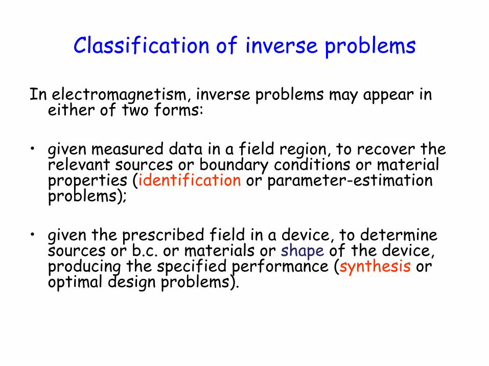
Classification of inverse problems

In electromagnetism, inverse problems may appear in either of two forms:

• given measured data in a field region, to recover the

relevant sources or boundary conditions or material properties (identification or parameter-estimation problems);

• given the prescribed field in a device, to determine sources or b.c. or materials or shape of the device, producing the specified performance (synthesis or optimal design problems).

Insidiousness of inverse problems From the mathematical viewpoint, following the Hadamard

definition (1923), well-posed problems (or properly, correctly posed problems) are those for which:

• a solution always exists; • there is only one solution; • a small change of data leads to a small change in the solution. Ill-posed problems, instead, are those for which: • a solution may not exist; • there may be more than one solution; • a small change of data may lead to a big change in the solution. The last property implies that the solution does not depend

continuously upon the data, which often are measured quantities and therefore are affected by noise or error.

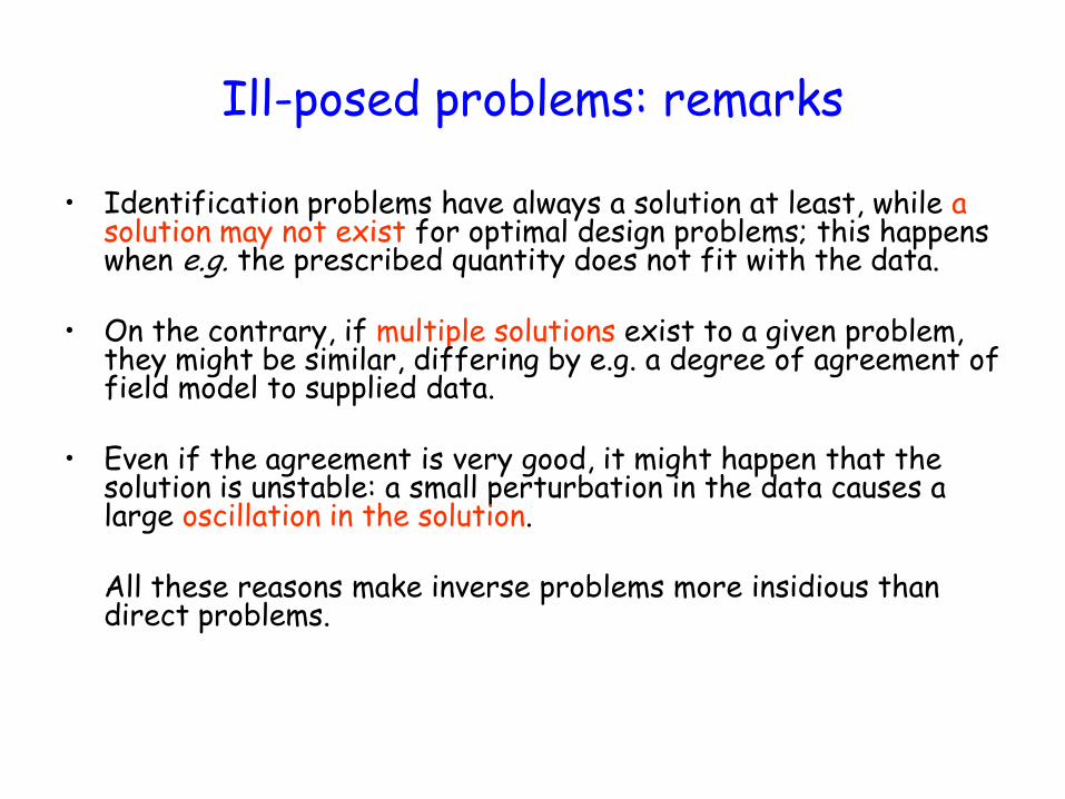
Ill-posed problems: remarks

• Identification problems have always a solution at least, while a solution may not exist for optimal design problems; this happens when e.g. the prescribed quantity does not fit with the data.

• On the contrary, if multiple solutions exist to a given problem, they might be similar, differing by e.g. a degree of agreement of field model to supplied data.

• Even if the agreement is very good, it might happen that the solution is unstable: a small perturbation in the data causes a large oscillation in the solution.

All these reasons make inverse problems more insidious than

direct problems.

Inverse problems and design problems

• Any design problem can be formulated in mathematical terms as an inverse problem.

• In particular, optimal shape design problems, which

are very popular in all branches of engineering, belong to a group of inverse problems where the purpose is to find the geometry of a device which can provide a prescribed behaviour or an optimal performance.

• The ultimate goal is to perform an automated optimal

design (AOD), when the solution is obtained automatically in terms of the required or best performance.

Solving an inverse problem

by minimising a functional

• In general, the nv unknowns x of an inverse problem are called design variables or degrees of freedom. The design variables may be geometric coordinates of the field region or values of sources or parameters characterizing the region.

• The solution to an inverse problem is generally performed by means of the

minimisation of a suitable function f(x) called objective function, or cost function, or design criterion. This function may represent some performance depending on the field, or simply the residual between computed and prescribed field values (error functional).

• In mathematical terms, the problem reads: given find where x0 is an initial guess. Properly speaking, it is a problem of unconstrained

minimisation; to be more meaningful, it is assumed that f is limited in W.

vn

0 Rx W

vn

xRx,xfinf W

Constrained minimisation

• The objective function should fulfil constraints, which may be expressed as equalities, inequalities and side bounds. Formally, the problem can be stated as follows:

given find subject to

• Constraints and bounds set the boundary of the

feasible region W associated with function f(x), and define implicitly its shape in the nv-dimensional design space.

vn

0 Rx W

vn

xRx,xfinf W

ci nixg ,...,1,0

ej njxh ,...,1,0

vkkk n,...,1k,ux

Insidiousness of minimisation

• Classical optimality requires the following first-order necessary condition, better known as Kuhn-Tucker theorem (1951):

Let be a local minimum point for f(x) and let f, gi , hj differentiable functions. Then, there exists a vector of multipliers such that

• This is a sufficient condition for to be a global minimum point if f(x) is a convex function and W is a convex region.

0~

,0~~

0~~~~~

11

iii

n

j

jnj

n

i

ii

xg

xhxgxfe

c

c

x~

ecnn~

x~

Usable and feasible

search direction S

0

0

SAg

SAf

Constrained minimization

0

0

SBg

SBf

Geometric interpretation

of KT conditions

(constraint g3 is not active in

x* and therefore 3=0)

Insidiousness of minimisation (2)

• In computational electromagnetism, it happens that functions f, gi and hj are known only numerically as a set of values at sample points; therefore, classical assumptions about differentiability and convexity cannot be assessed.

• In particular, when the assumption of convexity is not applicable, f might exhibit some local minima in addition to the global minimum.

• Moreover, the numerical approximation of the

gradient is time consuming; moreover, it is a potential source of fatal inaccuracies.

An alternative: evolutionary computing

• Darwinian evolution is intrinsically a robust search; it has become the model of a class of optimisation methods for the solution of real-life problems in engineering.

• The natural law of survival of the fittest in a given

environment is the model to find the best design configuration fulfilling given constraints.

• The principle of natural evolution inspired a large

family of algorithms that, through a procedure of self-adaptation in an intelligent way, lead to an optimal result (Goldberg, 1989).

Evolutionary computing (2)

• A primary advantage of evolutionary computing is its conceptual simplicity.

• A very basic pseudo-code of a typical algorithm:

i) initialize a population of individuals; ii) randomly vary individuals; iii) evaluate fitness of each individual; iv) apply selection; v) if the terminating criterion is fulfilled then stop, else go to step ii).

Evolutionary computing (3)

Evolutionary computing algorithms are:

• easy to implement;

• gradient-free;

• global-optimum oriented.

On the other hand, they are rather slow and costly, because of the high number of function evaluations required to converge.

An evolution strategy of lowest order

Evolution strategy mimics the survival of the fittest individual that is observed in nature. The flow-chart of an algorithm (in which a single parent generates a single offspring) is here presented.

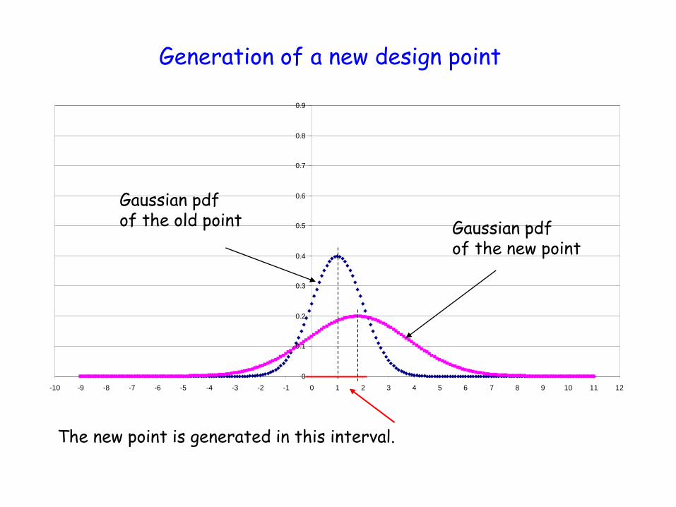
The new point is generated in this interval.

Generation of a new design point

0

0.1

0.2

0.3

0.4

0.5

0.6

0.7

0.8

0.9

-10 -9 -8 -7 -6 -5 -4 -3 -2 -1 0 1 2 3 4 5 6 7 8 9 10 11 12

Gaussian pdf of the old point Gaussian pdf

of the new point

Insidiousness of minimisation (3)

The No-Free Lunch (NFL) theorem (Wolpert and Macready, 1997)

There is no best algorithm,

whether or not it is evolutionary

Whatever an algorithm gains in performance on a class of problem, is necessarily lost by the same algorithm in the other problems

performance

average

dedicated algorithm

general-purpose algorithm

problem

FIELD-BASED OPTIMAL SHAPE DESIGN

Design vector x represents the geometry of the device to be synthesized. Generally, j-th objective function fj , j = 1,nf is a field-dependent quantity. The following mapping applies: The minimisation problem reads: find subject to nc field-dependent constraints In a problem of shape design, two aspects are always involved: the optimal synthesis of field s which takes place in the device, and the optimal design of device geometry x.

fj n,1j,xs,xfobjectivexsfieldxgeometry

f

n

jx

njxxsxf v ,1,,,inf W

ckk nkcxsxgxC ,1,,

Maxwell equations finite element analysis

Numerical solution to design problems: AOD

A procedure of AOD requires, as a rule, a routine for calculating the field, which is integrated in a loop with a routine optimising the objective function.

OPTIMISATION

ALGORITHM

Initial F.E. MESH

CONNECTIVITY

EVALUATOR

{X}1.0 {X}2.0

{X}

NONLINEAR

CONSTRAINTS

MESH

GENERATION

NONLINEAR

FIELD

ANALYSIS

F

physical

parameters geometrical

parameters

LINEAR

CONSTRAINTS

OPTIMUM

{X}

Numerical solution to design problems (2)

• The device to be optimised is represented by a numerical model in two or three dimensions (i.e. a grid of nodes and elements).

• The main flow of the computation is driven by the optimisation routine (e.g. evolution strategy). Starting from x0 , an iterative procedure updates the current design point xk in xk+1 .

• Given xk+1 , the routine of field analysis generates a new finite-

element grid, the field simulation is restarted and the evaluation of f(x) is so updated.

• If the procedure converges, the result could represent either a local minimum or the global minimum or simply a point better than the initial one, because f has decreased; in the latter case, a mere improvement (and not the optimisation) of f has been achieved.

Numerical solution to design problems (3)

• Usually, the analysis of field can be performed either by differential methods originated from Maxwell equations (finite-difference method, finite-element method), or by integral methods derived from Green theorem (boundary-element method).

• In turn, numerical optimisation can be achieved by means of

deterministic (i.e. gradient-based) methods or evolutionary (i.e. gradient-free) methods.

• Nowadays, most of commercially available codes devoted to

electromagnetic field simulation are based on the finite-element analysis (FEA): they proved, in fact, to offer a general-purpose and flexible tool of field simulation.

Numerical solution to design problems (4)

• Commercial FEA codes are equipped with a user interface, which enables the designer to develop a model in two or three dimensions by means of graphical operations only.

• These features make the simulation environment rather friendly

and easy to use; so, in practice, FEA has become the most popular tool, mainly in an industrial centre for R&D.

• The combination of any method for analysis and any method for

minimisation gives origin to a variety of iterative procedures for solving an optimal design problem.

Multiobjective formulation of a design problem

Often, in electromagnetic design, multiple objective functions should

be optimised simultaneously.

These problems belong to the category of multi-objective or multi-criteria. Their formulation is characterized by a vector of objective functions.

Formally, considering nv variables and nf objectives, one has: given , find subject to nc inequality and ne equality constraints and to 2nv side bounds

vn

0x fvnn

xFxxF ,,inf

ci n,1i,0xg ej n,1j,0xh

vkkk n,1k,ux

Mapping from design space to objective space

nv - dimensional nf - dimensional

Preference function formulation

Traditionally, the multiobjective problem is reduced to a single-objective one by means of a preference function , e.g. the weighted sum of the objectives: with should be minimised with respect to subject to the problem contraints.

The hierarchy attributed to the i-th objective can be modified by changing the corresponding weight ci . For a given set of weights, the relevant solution, if any, is assumed to be the optimum.

x

f

n

1i

ii xfcx

1c,1c0f

n

1i

ii

x vn

x

Paretian optimality (1)

The most general solution to the design problem is given by the front of

Pareto-optimal solutions

Solutions for which the decrease of an objective is not possible without the simultaneous increase of at least one of the other objectives

This means to have a family of solutions to be compared

Paretian optimality (2)

A solution is said to dominate another one if the first is better than the second with

respect to one objective, without worsening all the other objectives.

Two solutions are indifferent to each other if the first is better than the second for some objectives, while the second is better than the first in all the other objectives.

f1

f2

y1 y2

y3 y4

y5 y6

indifferent

indifferent

dominated (worse)

dominating (better)

Paretian optimality (3)

Given two solutions xj and xk

situation consequence

xj dominates xk xj is better than xk

xk dominates xj xk is better than xj

none of the two xj and xk are indifferent

Two key definitions

Let be an objective space. Then, a point is said to be Pareto optimal if no point exists

such that dominates .

Let be a vector of nf objectives, with design space and objective space : the set is the Pareto front (PF); the set is the Pareto set (PS).

fn

Y Yy

Yy~

y~F 1 yF 1

YX:xF

vn

X fn

Y

optimalParetoisyYy

xFXx

Correspondence between PF and PS

The PS topology depends on the Y to X inverse mapping: it might form e.g. a set of islands

In practice, the objective space Y is the control space

Metric criteria to identify non-dominated solutions in the design space X

Dominance dihedral

Orthogonal sector in the objective space:

• has its vertex at a given point y0 ; • contains all the points yk such that F-1(yk) dominates F-1(y0).

If the dihedral is empty, then F-1(y0) is said to be non-dominated.

y0

yk

U

R

A

f1

f2

Y

The objective space: a geometric interpretation in 2D

utopia point

nadir point

anti-utopia point

f

ni1 U,...,U,...,UU

fix

i n,1i,xfinfU

ideal objective vector

If Ui=Ui+1 , i=1,nf-1

then the optimisation problem is single-objective

1,1,,1,~~,~1 ffjjiii njnixxUxf A conflict exists

3Uf2Uf1

Uf32Uf1

Uf3Uf21

Uff

fUf

ffU

M

3333

2222

1111

fijn,1j

i n,1i,MmaxRf

Nadir point

Metric matrix (nf=3)

nf SO optimisations

Utopia point

HIGHER-ORDER DIMENSIONALITY nf>2

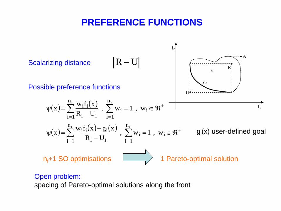
Scalarizing distance

Possible preference functions

UR

Open problem:

spacing of Pareto-optimal solutions along the front

gi(x) user-defined goal

i

n

1i

n

1i

iii

ii w,1w,UR

xfwx

f f

i

n

1i

n

1i

iii

iii w,1w,UR

xgxfwx

f f

nf+1 SO optimisations 1 Pareto-optimal solution

U

R

A

f1

f2

Y

PREFERENCE FUNCTIONS

Geometric classification of the PF in 2D (1)

Typical topologies of front

PF as a function of of nf -1 objectives:

Ad hoc optimisation algorithms

1n1nnfff

f,...,ff~

f~

Non-uniformly sampled PF (deceptive topology)

Non-linear objective functions

Geometric classification of the PF in 2D (2)

Multimodal optimisation problems

non-convex objective functions

local fronts, in addition to the global front

local front

global front

A solution j constraint-dominates a solution k, if any is true:

Handling constraints

j is feasible and k is not; j and k are both infeasible, but j has a smaller constraint violation; j and k are feasible and j dominates k.

Constraint-dominance principle (parameter-less)

Penalty function method (conventional) 0,)()()(1

2

i

n

i

ii rxgrxxc

Constrained MOOP

vfv n1nn11 x,..,xf .., , x,..,xf

Higher-level

information

Estimate a

weighting vector

fn1 w,...,w

SO optimisation problem

fn

11

iifwF

MO optimiser

Multiple trade-off

solutions found

Higher-level

information

Choose one solution

Problem

Solution

Classical methods

Pareto optimality

SO optimiser

f1

f2

f1

f2

Logical paths of classical and Paretian formulations

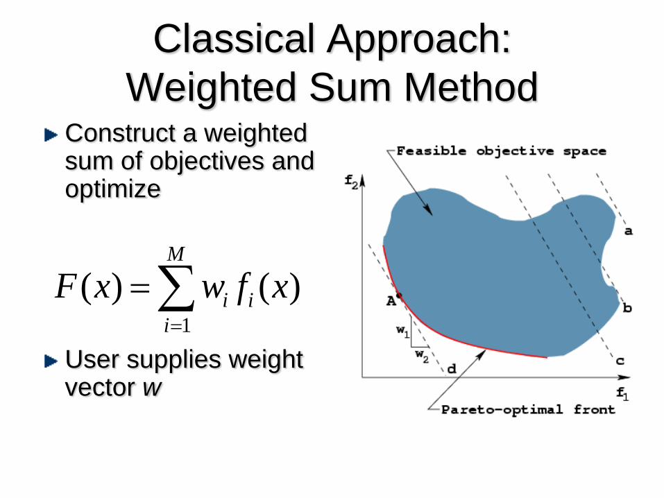
Classical Approach:

Weighted Sum Method Construct a weighted sum of objectives and optimize

User supplies weight vector w

1

( ) ( )M

i i

i

F x w f x

Difficulties with Classical Methods

Nonuniformity in Pareto-optimal

solutions

Inability to find some solutions

Epsilon-constraint method still

requires an -vector

jj ,

vn

ix

Rx,xfinf W

fjj n,1j,ij,xf

The -formulation reads:

given a set of nf-1 values

subject to

find

USING EVOLUTIONARY ALGORITHMS

• Population approach suits well to find multiple solutions

• Niche-preservation methods can be exploited to find diverse solutions

• Implicit parallelism helps provide a parallel search

• Shape of Pareto front is not a matter (e.g. non-convexity, disconnectedness)

Modify the fitness

computation

Emphasize non-dominated

solutions for convergence

Emphasize less-crowded

solutions for diversity

POPULATION-BASED APPROACH

WHAT TO CHANGE IN A BASIC GA ?

Elitist Non-dominated Sorting Genetic

Algorithm (NSGA-II)

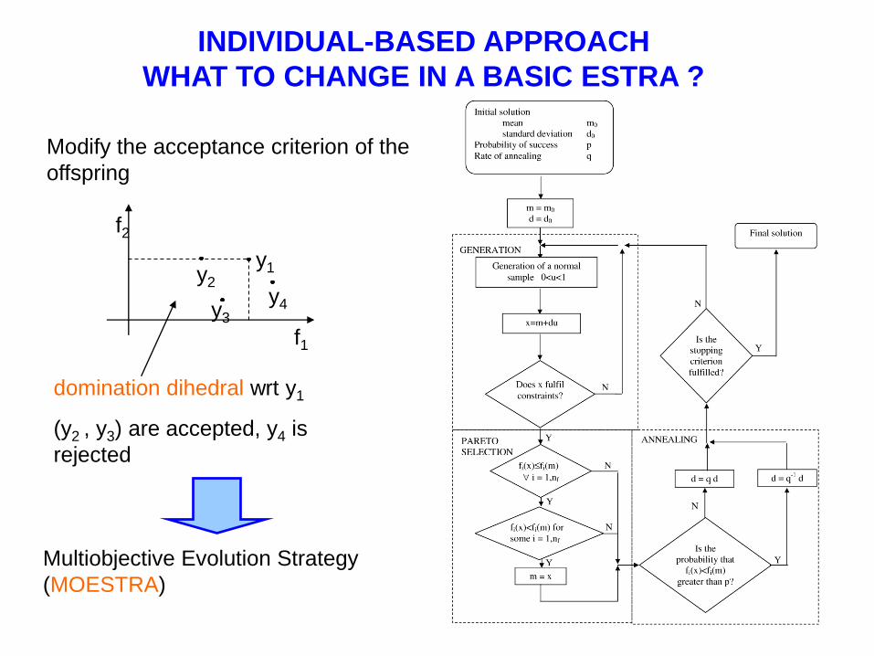
INDIVIDUAL-BASED APPROACH

WHAT TO CHANGE IN A BASIC ESTRA ?

Multiobjective Evolution Strategy

(MOESTRA)

f1

f2

y1 y2

y3 y4

(y2 , y3) are accepted, y4 is

rejected

domination dihedral wrt y1

Modify the acceptance criterion of the

offspring

Two main streams can be observed

•use approximation

techniques

•identify a surrogate model of

objectives and constraints

then

•use an evolutionary

algorithm to optimize

•preserve the use of FEA (very

flexible ! ) to solve the direct problem,

but

•reduce the solution time of field

analysis

•implement cost-effective strategies

well suited for an industrial

R&D centre

PRACTICAL METHODS TO SOLVE EMO IN

ELECTROMAGNETISM

SURROGATE MODELS

f

n

1j

jj

m

1i

iikk n,1k,xxxbxsxfss

sn

1j

jp

jjxx

j exxkriging model

Predictor formula

global basis function local basis function

ms+ns sampled points

Scalarizing methods

Combine the surrogates of multiple objectives into a preference

function; then, single-objective optimisation.

Non-scalarizing methods

consider the surrogate of each objective individually; then, non-

dominated solutions.

0j 2,0p j

CASE STUDY

Permanent-magnet generator for

automotive applications.

A very similar device was used as the

alternator on board of fast cars for

sport competitions.

Design problem: identify the shape of the device such that

• power loss in copper windings

• power loss in the iron core

are minimum.

W Wx

21

1

dxJxf

W Wx

22

dxBpxf

Constraint : load 500 W, no-load peak voltage 50 V , speed 9,000 rpm

W1 copper volume

W2 iron volume

NSGA-II AND MOESTRA IN ACTION

sampled Pareto front

prototype

NSGA-II: 20 individuals

MOESTRA: 1 individual

P. Di Barba and M. E. Mognaschi, “Industrial Design with Multiple Criteria: Shape Optimization of a

Permanent-Magnet Generator”, T-MAG, vol.45, 2009

NSGA-II and MOESTRA, after 6,300 s NSGA-II, after 10 gen.s

(2 runs, 20+20 ind.s)

Left: prototype solution, right: a Pareto optimal solution. Iron specific-loss curve.

Magnetization curve of iron core. Detail of the FE mesh.

NON-CONFLICTING MULTIPLE OBJECTIVES

An axisymmetric antenna

for magnetic induction tomography

Optimal design problem

Find the antenna shape, identified by variables (a,d,), such

that:

the magnetic field along the antenna axis (z>0) is

maximum, and simultaneously

the stray field behind the antenna (z<0) is minimum.

Frequency dependent field

NON-CONFLICTING MULTIPLE OBJECTIVES (II)

Optimisation results for f = 10 kHz

Optimisation results for f = 100 kHz

The optimum is unique (zero-dimensional Pareto front)

HIGHER-ORDER DIMENSIONALITY nf>2 (I)

Method of orthogonal projections

Unpractical for identifying P-optimal solutions

Effective for objective space representation

Design points are mapped in all possible 2D subspaces

ji,n,1j,i,f,f fji

HIGHER-ORDER DIMENSIONALITY nf>2 (II)

Design variables rotor inner radius rotor slot width

Objectives static torque, to be max torque ripple, to be min radial force (friction), to be min

The device Electrostatic microactuator

E. Costamagna, P. Di Barba, A. Savini, Shape design of a MEMS device by Schwarz-

Christoffel numerical inversion and Pareto optimality, COMPEL, vol. 27, 2008

OPEN PROBLEMS IN EMO: BENCHMARKING

Some goals of benchmarking : •Move from test problems to industrial benchmarks •Investigate topological properties of the PF (convex/non-convex, connected/non-connected, uniformly/non-uniformly spaced) •Define suitable metrics to measure the distance of a given solution point from the front

In EMO, evaluating the performance of an optimisation algorithm and assessing results is a challenging task.

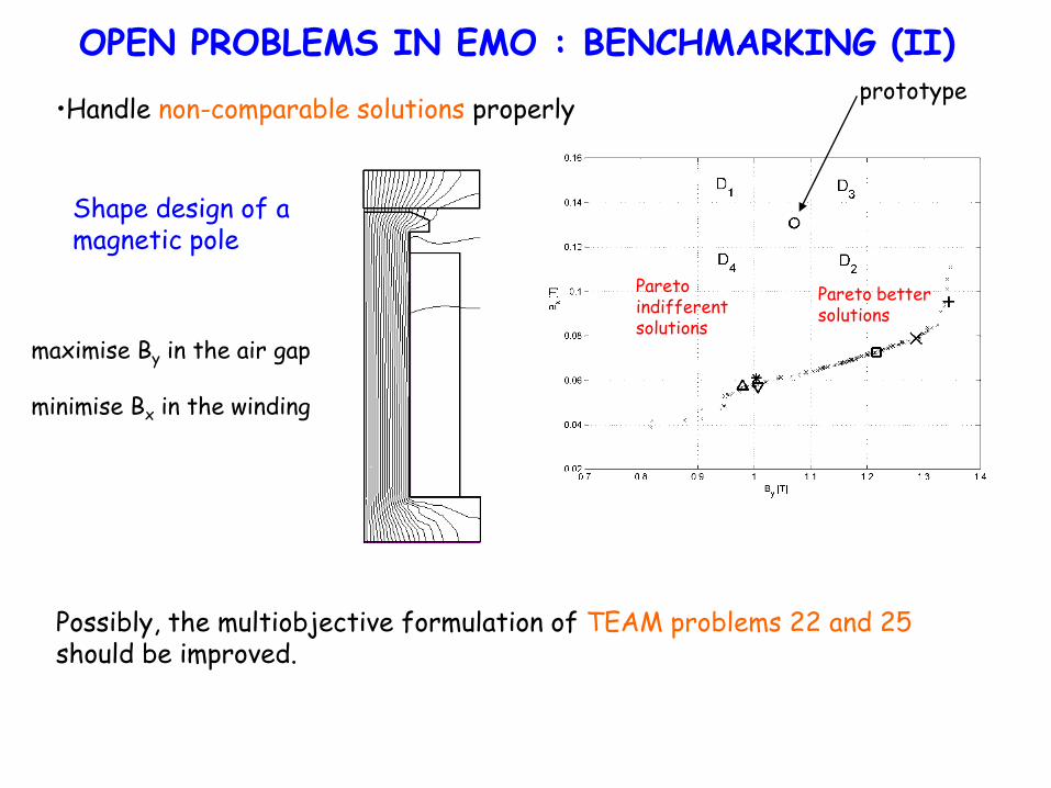
Possibly, the multiobjective formulation of TEAM problems 22 and 25 should be improved.

•Handle non-comparable solutions properly

prototype

maximise By in the air gap minimise Bx in the winding

Shape design of a magnetic pole

Pareto better solutions

Pareto indifferent solutions

OPEN PROBLEMS IN EMO : BENCHMARKING (II)

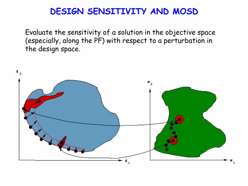
DESIGN SENSITIVITY AND MOSD

Evaluate the sensitivity of a solution in the objective space (especially, along the PF) with respect to a perturbation in the design space.

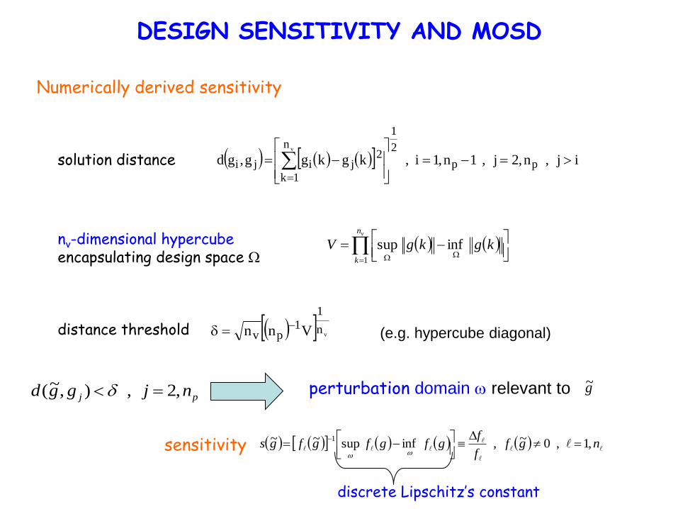
DESIGN SENSITIVITY AND MOSD

Numerically derived sensitivity

ngf

f

fgfgfgfgs ,1,0~,infsup~~ 1

ij,n,2j,1n,1i,kgkgg,gd pp

2

1n

1k

2jiji

v

vn

1

1pv Vnn

d

WW

vn

k

kgkgV1

infsup

solution distance

discrete Lipschitz’s constant

nv-dimensional hypercube encapsulating design space W

distance threshold

pj njggd ,2,),~( d perturbation domain relevant to

sensitivity

(e.g. hypercube diagonal)

g~

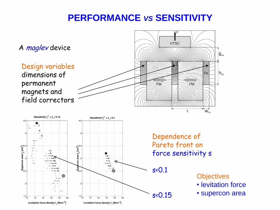
PERFORMANCE VS SENSITIVITY

A maglev device

Design variables dimensions of permanent magnets and field correctors

Dependence of Pareto front on force sensitivity s s<0.1 s<0.15

Objectives

• levitation force

• supercon area

The adaption rate 0<<1 of the

FE mesh is ruled by the

annealing operator of a basic

evolution strategy.

A low-cost mesh is generated when a large search radius is taken on and, conversely, a finer mesh is generated when a small region is investigated.

A multi-scale evolutionary search

qlog

dlogdlogn 0f

n

km

n

km1k maxmin

qlog

dlogkdlogkm 0

d0 initial search tolerance

df final search tolerance

k iteration index

q annealing rate

CASE STUDY

Fixed vs variable adaption

(fixed =0.15, variable 0.02<<0.2)

x=[10.33, 1.01, 2.30, 7.99, 2.87] mm

f=[4.55, 160] mW

x=[10.87, 0.97, 2.11, 6.83, 3.05] mm

f=[4.36, 150] mW

Stopping criterion: search tolerance < 10-6

larger search radius

CASE STUDY (II)

Objective function history

Fixed adaption Variable adaption

CASE STUDY (III)

User-defined accuracy: the optimisation stops when 0k,2,1i,f

f)k(

i0

kii

x=[10.18, 1.06, 2.38,

8.03, 2.95] mm

1=0.75, 2=0.4

x=[10.81, 0.99, 2.09,

6.84, 3.07] mm

1=0.65, 2=0.36

k=43

k=49

Prescribed = 0.75

CASE STUDY (IV)

User-defined time: the optimisation stops after e.g. 1 hour

x=[9.70, 1.21, 2.40, 7.93, 3.00] mm

f1=5.5 mW, f2=179.3 mW 11 iterations done in 1 hour

Improvement: 20% for f1 , 60% for f2

Fixed adaption

Variable adaption

CASE STUDY (V)

An a priori method to provide the designer with a single optimum. Each player minimises his own objective by varying a single variable and assuming that the values of the remaining n-1 objectives are fixed by the other n-1 players. If it happens that no player can further reduce his objective, it means that the system has converged to an equilibrium.

AN ALTERNATIVE: NASH GAMES

ni1i ...... WWWWW

Wni1 x~,...,x~,...,x~

n1ii1i1i x~,...,x~,x~,x~,...,x~f

n,...,1ix~,...,x~,x,x~,...,x~finf n1ii1i1ix

ii

W

Then, a point

Let W and Wi be the global design space and the design space of the i-th objective,

such that

is a Nash equilibrium (NE) if

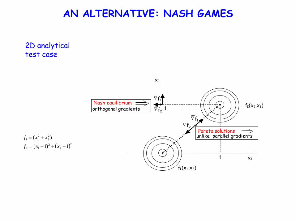
2D analytical test case

1

1

x 1

x 2

f 1 (x 1 ,x 2 )

f 2 (x 1 ,x 2 )

Pareto solutions unlike parallel gradients

Nash equilibrium orthogonal gradients

2 f

2 f 1 f

1 f

AN ALTERNATIVE: NASH GAMES

22

2

12

2

2

2

11

1)1(

)(

xxf

xxf

NASH GAMES: NUMERICAL IMPLEMENTATION

Player 1 optimizes f1(x1,x2) acting on x1 and receiving x2 from player 2 at the previous iteration; then, player 1 sends the result to player 2.

Player 2 optimizes f2(x1,x2) acting on x2 and receiving x1 from player 2 at the previous iteration; then, player 2 sends the result to player 1.

The game is over (Nash equilibrium) when neither player 1 nor player 2 can further improve their objectives.

Design variables : height and width of magnet

PM THREE-PHASE MOTOR

P. Di Barba, Strategies of game theory for the automated optimal design in electromechanics, Intl J of Applied Electromagnetics and Mechanics 27 (2008) 1-21

Air gap

Laminated rotor

Laminated stator

Slot

NE initial (a)

NE final (b)

NE final (c)

o global P-solutions ◊ local P-solutions

Objectives for no-load operation: cogging torque (to be min), air-gap radial induction (to be max)

Design variables :

(a1,a2,a3,a4)

The problem reads: find the time-dependent family of non-dominated solutions from t = 0+ to steady state such that

• air-gap induction is maximum

• power loss in the winding is minimum

under the constraint that

the power loss in the pole and the core at a given time instant (t=10-2t) is not greater than the power loss in the winding.

Time constant depends on geometry

FROM STATIC TO DYNAMIC PARETO FRONTS

Shape design of a magnetic pole

p

2

k21 n,1k,kinf

t

p3412 n,1k,kaka,kakamink

time-unconstrained (circle) and time-constrained (star) fronts

time-unconstrained (circle) and time-constrained (star) fronts

The energy constraint, active in the first part of the transient magnetic diffusion, influences the Pareto front shape at any subsequent time instant !

P. Di Barba, A. Lorenzi, A. Savini, Dynamic Pareto fronts and optimal control of geometry in a problem of transient magnetic diffusion, IET Science, Measurement and Technology, 2008, vol.2, no.3, 114-121

Objective space at t = t Objective space at steady state

FROM STATIC TO DYNAMIC PARETO FRONTS (II)

Geometry and flux lines of a non-dominated solution at steady state (time-unconstrained PF) :

f1 = 846.031 mT, f2 = 40.073 mT (prescribed f1 = 850 mT); a1 = 32 mm, a2 = 45 mm, a3 = 6 mm, a4 = 25 mm.

Geometry and flux lines of a non-dominated solution at steady state (time-constrained PF) :

f1 = 855.773 mT, f2 = 84.628 mT (prescribed f1 = 850 mT); a1 = 22 mm, a2 = 72 mm, a3 = 19 mm, a4 = 24 mm.

FROM STATIC TO DYNAMIC PARETO FRONTS (III)

Also the

solution

shape is

different !

Time unconstrained

Time constrained

FROM STATIC TO DYNAMIC PARETO FRONTS (IV)

If the energy constraint is not active, the problem becomes adynamic.

MOVING ALONG THE PARETO FRONT

John necessary condition:

Pareto optimal solution satisfies

1. and

2.

Requires differentiable objectives and constraints

Outlines the existence of some common properties among Pareto-optimal solutions

If objectives fi(x), i=1,nf are convex and W is a convex region,

the condition is sufficient too.

cf

n

1k

kk

n

1i

ii x~gx~f

ckk n,1k,0x~g

x~

MOVING ALONG THE PARETO FRONT (II)

knee

min f1

min f2

P. Di Barba, M.E. Mognaschi, Sorting Pareto solutions: a principle of optimal design for electrical machines, COMPEL, vol. 28, 2009

BEYOND EMO

Evolutionary, genetic and migratory algorithms, often employed in MOO, are powerful, but affected by some inherent limits, the most evident of which is the absence of theoretical proofs of convergence.

BEYOND EMO (II)

Individuals of a population-based method of optimisation run towards improvement through a randomness guided by a set of possible heuristics.

An alternative way is developing a statistical method to identify the regions of the X space – the most interesting one to the designer – which are more likely to map onto P-optimal solutions.

The designer, then, should be provided not with a large collection of supposed-optimal individuals, but with a distribution of probability in the X space, which yields optimal configurations with a given degree of certainty.

BEYOND EMO (III)

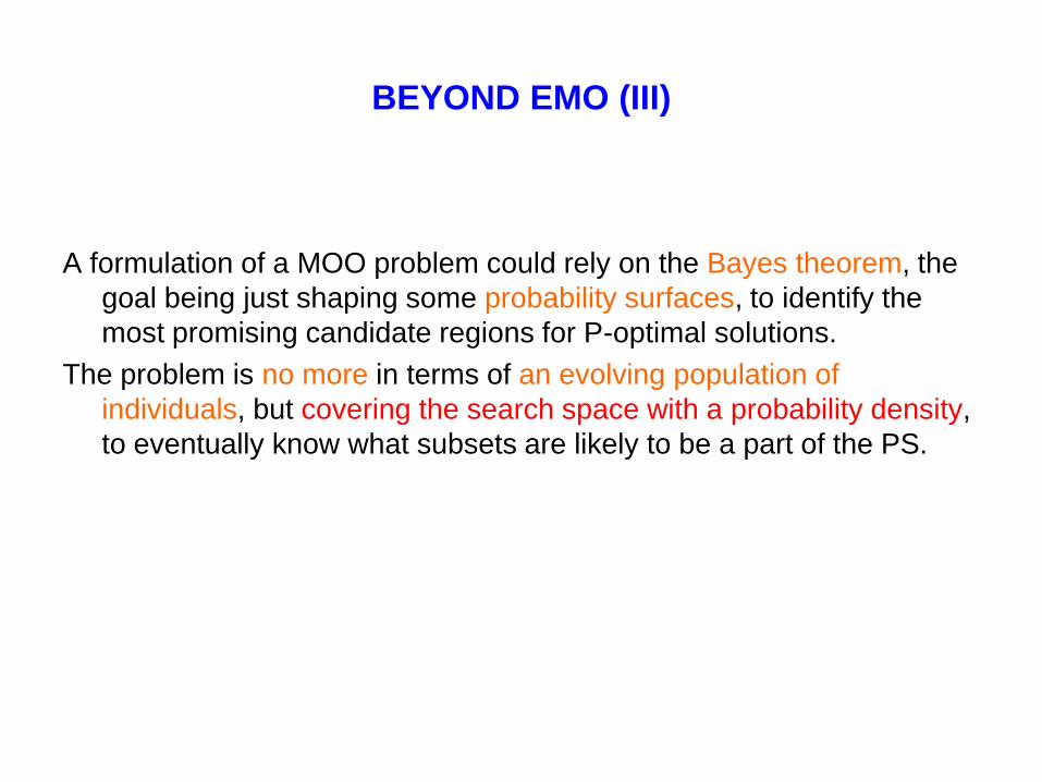
A formulation of a MOO problem could rely on the Bayes theorem, the

goal being just shaping some probability surfaces, to identify the

most promising candidate regions for P-optimal solutions.

The problem is no more in terms of an evolving population of

individuals, but covering the search space with a probability density,

to eventually know what subsets are likely to be a part of the PS.

BEYOND EMO (IV)

Let an optimisation process have already produced some individuals, among which the non-dominated ones have been ranked out.

Then, given a point belonging to the X space, its probability of belonging to the P-set is proportional to its probability of mapping onto a non-dominated point in the Y space, times the probability that a non-dominated point be P-optimal.

BAYESIAN IMAGING AND MO PROBLEMS

Ixp

IypI,yxpI,xyp

“x belongs to the PS”

“y belongs to the PF”

Given the a priori information I and defined the two propositions:

normalizing constant

stopping term: the probability for any point y to belong to the PF

forward mapping term

backward mapping term the Bayes theorem reads

Xx,x

Yy,y

BAYESIAN IMAGING AND MO PROBLEMS

SHAPE DESIGN OF A LINEAR ACTUATOR

521 ,x,,h,ha Wa Design vector

aCinfa W

aVcaVcaC coppercopperironiron

aFsup ya W

0gg

yy

a'WaF

0y

a

BaBsup

w

W

Find

and

subject to

OPTIMISATION RESULTS (I)

F-space sampling (circle), with relevant PF (star), and PF derived after optimisation (triangle).

OPTIMISATION RESULTS (II)

PS projected on the (h1,h2) plane after optimisation

Other optimal solutions can be generated at zero cost, by means of new extractions, until the requirements of the designer in terms of likelihood are met.

Pareto optimality and MEMS design Fostered by the development of new technologies, micro-electro-mechanical systems (MEMS) are massively present on board of vehicles, within information equipment, in manufacturing systems as well as in medical and healthcare equipment. The miniaturisation of electromechanical systems will impact our society as deeply as did the mass production of electronic systems in the latest forty. However, only in more recent times has the design of MEMS been approached in a systematic way employing automated optimal design. Accordingly, the design problem is set up as a problem of non-linear multi-objective optimization of design criteria subject to a set of constraints. The approach implies suitable computational environments made available by the progress in artificial intelligence, where modelling tools are integrated with soft computing tools .

Comb drive MEMS

3D geometry

10 fixed electrodes (u=1V)

9 movable electrodes (u=0 V)

grounded substrate

fixed electrode

(supplied)

x-direction

movable

electrode

(grounded)

ground plane

dielectric gas

g

wm

g/2 g/2

wf

z1 z2

hm

s.a.

hf

z

y x

s.a.

Comb drive MEMS: cross-sectional view

Comb drive MEMS

Field analysis

Laplace equation + Maxwell stress tensor

Mesh characteristic Value

Minimum element quality 0.2818

Average element quality 0.7927

Tetrahedral elements 170840

Triangular elements 34468

Edge elements 2812

Vertex elements 172

Maximum element size 2.64 μm

Minimum element size 0.0264 μm

Resolution of curvature 0.2

Resolution of narrow regions 1

Maximum element growth rate 1.3

Comb drive MEMS - FE mesh

Comb drive MEMS

Force simulation

Approximately, it turns out to be:

Fz=k(z-z0)

Drive force Fx vs x-directed displacement (main effect)

Levitation force Fz vs z-directed displacement (side effect)

movable electrode equilibrium height z0

“electrostatic spring” Constant k

Comb drive MEMS - Optimal design problem

Optimal shape design problem The goal of the optimal shape design problem is to find the family of geometries which maximise the x-directed drive force between movable and fixed electrodes, and simultaneously mimimise the z-directed levitation force (electrostatic spring effect). Four-dimensional design space Design variables: width and height of movable and fixed electrodes, respectively. Design vector a = (wm,wf,hm,hf). Range: from 2 to 8 m. Discrete-valued (step 0.1 m).

Comb drive MEMS - Optimal design problem (II)

Two-dimensional objective space Vector of objective functions F = (f1,f2) with drive f1(a) = Fx(x,a) for z = 0 and -13 ≤ x ≤ 0 m, to be maximised with respect to a, levitation f2(a) = Fz(z,a) for x = -13 m and 0 ≤ z ≤ 4 m, to be minimised with respect to a. Both f1 and f2 are subject to the solution of the field analysis problem.

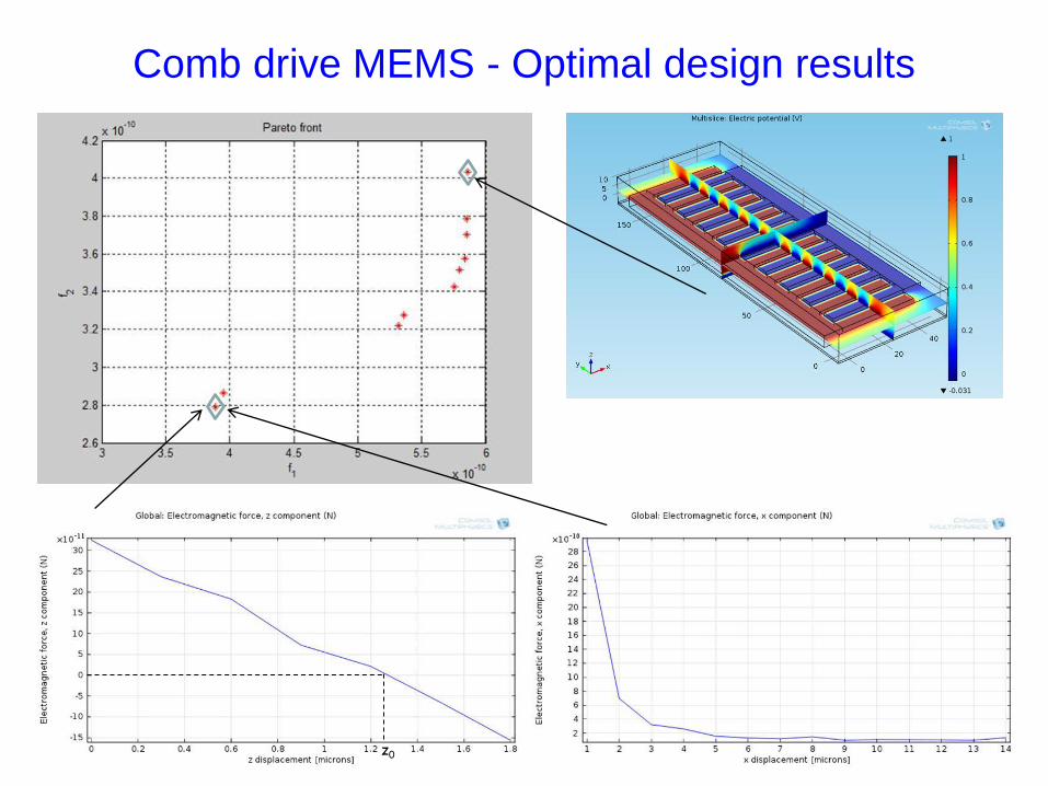
Comb drive MEMS - Optimal design results

z0

Comb drive MEMS - Optimal design results

X and F coordinates of individuals in the final generation

Width of mobile fingers wm [µm]

Width of fixed fingers

wf [µm]

Height of mobile fingers

hm [µm]

Height of fixed fingers

hf [µm]

Fx drive force

[N] x*10-10

Slope of Fz vs. z

[Nm-1] x*10-10

6 6 6.2 6.1 3.8848 2.7915

7.7 7.8 7.7 7.8 5.8568 4.0328

7.1 7.3 7.5 7.4 5.3189 3.2187

6.1 6.1 6.2 6.1 3.9496 2.862

7.6 7.7 7.8 7.9 5.8543 3.7876

7.7 7.7 7.8 7.8 5.8491 3.702

7.6 7.8 7.7 7.8 5.8385 3.5745

7.1 7.2 7.5 7.4 5.3614 3.2781

7.5 7.7 7.7 7.8 5.7529 3.4235

7.7 7.8 7.7 7.8 5.7975 3.5168

CONCLUSION

While there have been significant improvements in the capabilities in the area of MO design, the uptake by industrial designers has been somewhat limited. There are, possibly, two reasons for this.

The first is that the evidence, at the industrial level, that computer-based optimisation processes can actually enhance a designer’s ability to create a better product has been lacking.

The second relates to the fact that most optimisation packages currently available only handle a single objective and a limited number of design variables.

In fact, suitable optimisation systems, with no restriction in the size of the design space to be explored, and with simple and flexible expressions of objectives and constraints, would help match the needs of the designer.

P. Di Barba, Multiobjective Shape Design in Electricity and Magnetism, Springer, 2010.